Matching with Text Data: An ExperimentalEvaluation of Methods for Matching

Documents and of Measuring Match Quality

Reagan Mozer∗1, Luke Miratrix1, Aaron Russell Kaufman1, and L. JasonAnastasopoulos2

1Harvard University2University of Georgia

March 15, 2019

Abstract

Matching for causal inference is a well-studied problem, but standard methods failwhen the units to match are text documents: the high-dimensional and rich natureof the data renders exact matching infeasible, causes propensity scores to produce in-comparable matches, and makes assessing match quality difficult. In this paper, wecharacterize a framework for matching text documents that decomposes existing meth-ods into: (1) the choice of text representation, and (2) the choice of distance metric.We investigate how different choices within this framework affect both the quantity andquality of matches identified through a systematic multifactor evaluation experimentusing human subjects. Altogether we evaluate over 100 unique text matching meth-ods along with 5 comparison methods taken from the literature. Our experimentalresults identify methods that generate matches with higher subjective match qualitythan current state-of-the-art techniques. We enhance the precision of these results bydeveloping a predictive model to estimate the match quality of pairs of text documentsas a function of our various distance scores. This model, which we find successfullymimics human judgment, also allows for approximate and unsupervised evaluation ofnew procedures in our context. We then employ the identified best method to illustratethe utility of text matching in two applications. First, we engage with a substantivedebate in the study of media bias by using text matching to control for topic selectionwhen comparing news articles from thirteen news sources. We then show how condi-tioning on text data leads to more precise causal inferences in an observational studyexamining the effects of a medical intervention.

Keywords: high-dimensional matching, text analysis, topic modeling, news media

∗Corresponding Author: Reagan Mozer (email: rmozer@g.harvard.edu)

1

arX

iv:1

801.

0064

4v7

[st

at.M

E]

13

Mar

201

9

1 Introduction

Recently, Roberts et al. (2018) introduced an approach for matching text documents in order

to address confounding in observational studies of substantive and policy-relevant quantities

of interest. Matching is a statistical tool primarily used to facilitate causal inferences about

the effects of a particular treatment, action, or intervention from non-randomized data in the

presence of confounding covariates (Rubin, 1973b; Rosenbaum, 2002; Rubin, 2006; Stuart,

2010). The principles behind matching can also be used to create sharp, targeted comparisons

of units in order to, for example, create more principled rankings of hospitals (Silber et al.,

2014). The core idea of matching is to find sets of units from distinct populations that are

in all ways similar, other than some specific aspects of interest; one can then compare these

remaining aspects across the populations of interest to ascertain differences foundational to

these populations. In short, matching provides a strategy for making precise comparisons

and performing principled investigations in observational studies.

Though widely used in practice, matching is typically used in settings where both the

covariates and outcomes are well-defined, low-dimensional quantities. Text is not such a

setting. With text, standard contrasts of outcomes between groups may be distorted es-

timates of the contrasts of interest due to confounding by high-dimensional and possibly

latent features of the text such as topical content or overall sentiment. How to best capture

and adjust for these features is the core concern of this work. In particular, we consider

the problem of matching documents within a corpus made up of distinct groups (e.g., a

treatment and control group), where interest is in finding a collection of matched documents

that are fundamentally “the same” along key dimensions of interest (in our first application,

for example, we find newspaper articles that are about the same events and stories). These

matched documents can then be used to make unbiased comparisons between groups on

external features such as rates of citation or online views, or on features of the text itself,

such as sentiment. In the case where group membership can be thought of as the receipt

of a particular intervention (e.g., documents that were censored vs. not, such as in Roberts

et al., 2018), this allows us draw causal inferences about effects of interest.

This paper makes three contributions to guide researchers interested in this domain.

2

Our first contribution is a deconstruction and discussion of the elements that constitute

text matching. This formulation identifies a series of choices a researcher can make when

performing text matching and presents an approach for conceptualizing how matching can

be used in studies where the covariates, the outcome of interest, or both are defined by

summary measures of text. Our second contribution is to investigate these choices using a

systematic multifactor human evaluation experiment to examine how different representa-

tions and distance metrics correspond to human judgment about document similarity. Our

experiment explores the efficiency of each combination of choices for matching documents

in order to identify the representations and distance metrics that dominate in our context

in terms of producing the largest number of matches for a given dataset without sacrificing

match quality. We also present a general framework for designing and conducting systematic

evaluations of text-matching methods that can be used to perform similar investigations in

different contexts. Our third contribution is twofold.

First, we present a novel application of template matching (Silber et al., 2014) to compare

news media organizations’ biases, beyond choices of which stories to cover, in order to engage

with a running debate on partisan bias in the news media. Through template matching

on text, we identify similar samples of news articles from each news source that, taken

together, allow for a more principled (though not necessarily causal) investigation of how

different news sources may differ systematically in terms of partisan favorability. In our

second application, we illustrate the utility of text matching in a more traditional causal

inference setting, namely, in an observational study evaluating the causal effects of a binary

treatment. Here we demonstrate how matching on text obtained from doctors’ notes can be

used to improve covariate balance between treatment and control groups in an observational

study examining the effects of a medical intervention. We further discuss how researchers

might leverage text data to strengthen the key assumptions required to make valid causal

inferences in this non-randomized context.

Our work builds on Roberts et al. (2018), the seminal paper in this literature, which

introduces text matching, operationalizing the text data by using topic modeling coupled

with propensity scores to generate a lower-dimensional representation of text to match on.

They also present several applications that motivate the use of text matching to address

3

confounding and describe several of the methodological challenges for matching that arise in

these settings. Specifically, Roberts et al. (2018) discuss the limitations of direct propensity

score matching and coarsened exact matching (CEM) on the raw text for matching with

high dimensional data and introduce Topical Inverse Regression Matching (TIRM), which

uses structural topic modeling (STM) (Roberts et al., 2016) to generate a low-dimensional

representation of a corpus and then applies CEM to generate matched samples of documents

from distinct groups within the corpus. Building upon this work, we develop a general

framework for constructing and evaluating text matching methods. This allows us to consider

a number of alternative matching methods not considered in Roberts et al. (2018), each

characterized by one representation of the corpus and one distance metric. Within this

framework, we also present a systematic approach for comparing different matching methods

through our evaluation experiment, which identifies methods that can produce more matches

and/or matches of higher quality than those produced by TIRM. Overall, we clarify that there

is a tradeoff between match quality and the number of matches, although many methods do

not optimize either choice.

2 Background

2.1 Notation and problem setup

Consider a collection of N text documents, indexed by i = 1, . . . , N , where each document

contains a sequence of terms. These documents could be any of a number of forms such as

news articles posted online, blog posts, or entire books, and each document in the dataset

need not be of the same form. Together, these N documents comprise a corpus, and the

set of V unique terms used across the corpus define the vocabulary. Each term in the

vocabulary is typically a unique, lowercase, alphanumeric token (i.e., a word, number, or

punctuation mark), though the exact specification of terms may depend on design decisions

by the analyst (e.g., one may choose to include as terms in the vocabulary all bigrams

observed in the corpus in addition to all observed unigrams). Because the number and

composition of features which may be extracted from text is not well defined, documents

4

are generally regarded as “unstructured” data in the sense that their dimension is ex ante

unknown.1 To address this issue, we impose structure on the text through a representation,

X, which maps each document to a finite, usually high-dimensional, quantitative space.

To make principled comparisons between groups of documents within the corpus, we

borrow from the notation and principles of the Rubin Causal Model (RCM) (Holland, 1986).

Under the RCM, each document has an indicator for treatment assignment (i.e., group mem-

bership), Zi, which equals 1 for documents in the treatment group and 0 for documents in

the control group. Interest focuses on estimating differences between these groups on an

outcome variable, which, under a causal view, would take the value Yi(1) if document i is in

the treatment group and Yi(0) if document i is in the control group. These outcomes may

be separate from the text of the document (e.g., the number of times a document has been

viewed online) or may be a feature of the text (e.g., the length of the document or level of pos-

itive sentiment within the document).2 Credible and precise causal inference revolves around

comparing treated and control documents that are as similar as possible. However, in obser-

vational studies, Zi is typically not be randomly assigned, leading to systematic differences

between treatment and control groups. Matching is a strategy that attempts to address this

issue by identifying samples of treated and control documents that are comparable on covari-

ates in order to approximate random assignment of Zi (i.e., to satisfy Zi ⊥⊥ (Yi(0), Yi(1))|Xi)

(Rosenbaum, 2002; Rubin, 2006). Under this key assumption of “selection on observables,”

which states that all covariates that affect both treatment assignment and potential outcomes

are observed and captured within X, comparisons of outcomes between matched samples can

be used to obtain unbiased estimates of the quantities of interest (Rosenbaum, 2002). For

example, in our second application examining the effects of a medical intervention, we argue

that matching on both a set of numerical covariates and the text content of the patients

chart allows us to identify two groups of patients, one treated and one not, that are similar

enough on pre-treatment variables such that any systematic differences in their outcomes

can be plausibly attributed to the impact of the intervention.

1In particular, the number and composition of features which may be extracted from a given corpus isnot well-defined and may vary depending on researcher focus.

2In the latter case, care must be taken to ensure the features of the representation X used to define thecovariates are suitably separated from features that define the potential outcomes. This issue is discussedfurther in Section 3 and in Appendix A.4.

5

These causal inference tools can be used more broadly, however, to produce clearly defined

comparisons of groups of units even when a particular intervention is not well-defined. For

example, Silber et al. (2014) introduces template matching as a tool for comparing multiple

hospitals that potentially serve different mixes of patients (e.g., some hospitals have a higher

share of high-risk patients). The core idea is to compare like with like: by comparing hospitals

along an effective “score card” of patients, we can see which hospitals are more effective, on

average, given a canonical population. In general, we focus on this general conception of

matching, recognizing that often in text there is no treatment that could, even in concept, be

randomized. For example, a comparison of style between men and women could not easily

be construed as a causal impact. Nevertheless, the framing and targeting of a controlled

comparison, a framing inherent in a causal inference approach, can still be useful in these

contexts. This broader formulation of matching is used in our first application in Section 5

investigating different aspects of bias in newspaper media.

2.2 Promises and pitfalls of text matching

Matching methods generally consist of five steps: 1) identify a collection of potential con-

founders (covariates) that would compromise any causal claims if they were systematically

different across the treatment groups, 2) define a measure of distance (or similarity) to deter-

mine whether one unit is a good match for another, 3) match units across groups according to

the chosen distance metric, 4) evaluate the quality of the resulting matched samples in terms

of their balance on observed covariates, possibly repeating the matching procedure until suit-

able balance is achieved, and 5) estimate treatment effects from these matched data (Stuart,

2010). Different choices at each step of this process produce an expansive range of possible

configurations. For instance, there are distance metrics for scalar covariates (Rubin, 1973b),

for multivariate covariates summarized through a univariate propensity score (Rosenbaum

and Rubin, 1983, 1985), and multivariate metrics such as the Mahalanobis distance metric

(Rubin, 1978; Gu and Rosenbaum, 1993).

Similarly, there is a large and diverse literature on matching procedures (Rosenbaum,

2002; Rubin, 2006), and the choice of procedure depends on both substantive and method-

ological concerns. Some procedures match each unit in the treatment group to its one

6

“closest” control unit and discard all unused controls (e.g., one-to-one matching with re-

placement), while other procedures allow treated units to be matched to multiple controls

(e.g., ratio matching; Smith, 1997) and/or matching without replacement (e.g., optimal

matching; Rosenbaum, 1989). Match quality is often evaluated with a number of diagnostics

that formalize the notion of covariate balance such as the standardized differences in means

of each covariate (Rosenbaum and Rubin, 1985). Unfortunately, determinations of what

constitutes “suitable” balance or match quality are often based on arbitrary criteria (Imai

et al., 2008; Austin, 2009), and assessing whether a matching procedure has been successful

can be quite difficult. That being said, once a suitable set of matches is obtained, one can

then typically analyze the resulting matched data using classic methods appropriate for the

type of data in hand. Stuart (2010) outlines a number of common analytical approaches.

The rich and high-dimensional nature of text data gives rise to a number of unique

challenges for matching documents using the standard approach described above. From a

causal inference perspective, in many text corpora there is going to be substantial lack of

overlap, i.e., entire types of documents in one group that simply do not exist in the other

groups. This lack of overlap is exacerbated by the high-dimensional aspect of text: the richer

the representation of text, the harder it will be to find documents similar along all available

dimensions to a target document (D’Amour et al., 2017). This makes the many design

decisions required to operationalize text for matching such as defining a distance metric and

implementing a matching procedure especially challenging. Distance metrics must be defined

over sparse, high-dimensional representations of text in a manner that captures the subtleties

of language. If these representations are overly flexible, standard matching procedures can

fail to identify good (or any) matches in this setting due to the curse of dimensionality.

Lack of overlap can come from substantive lack of overlap (the documents are inherently

different), but also aspects of the text representation that are not substantive (this is akin to

overfitting the representation model). Ideally a good representation and distance metric will

preserve the former but not the latter. All of the matching procedures discussed in this work

can be thought of as carving out as many high quality matches as they can find, implicitly

setting parts of the corpus aside to have good comparisons across groups. This is in effect

isolating (Zubizarreta et al., 2014) a focused comparison within a larger context. In a causal

7

context, this can shift the implied estimand of interest to only those units in the overlap

region. For further discussion of the approaches commonly used to address overlap issues,

see, for example, Fogarty et al. (2016); Dehejia and Wahba (2002); Stuart (2010).

In addition to these difficulties, the rich nature of text data also provides an opportu-

nity in that it lends itself to more straightforward, intuitive assessments of match quality

than are typically possible with quantitative data. Specifically, while it is difficult to inter-

pret the quality of a matched pair of units using numerical diagnostics alone due to being

high dimensional, the quality of a matched pair of text documents is generally intuitive to

conceptualize. With text data, human readers can quickly synthesize the vast amount of

information contained within the text and quantify match quality in a way that is directly

interpretable. Thus, when performing matching with text data, final match quality can be

established in a manner that aligns with human judgment about document similarity. This

is a version of “thick description,” discussed in Rosenbaum (2010, pg. 322). This also allows

for comparing different matching methods to each other in order to find methods that, po-

tentially by using more sparse representations of text or more structured distance measures,

can simultaneously find more matched documents while maintaining a high degree of match

quality.

2.3 Different types of text-based confounding

Text is quite multifaceted, but that does not necessarily mean that the researcher needs to

attend to all aspects of the text in order to appropriately control for any confounding. The

confounding feature of the text may be superficial and reducible to keywords, for example

whether a news story covers politics, or it may be latent and difficult to deterministically

measure, like a news story’s ideological content.

In the simplest case, for example, consider a study with a single confounding feature that

affects both assignment to treatment and the outcome of interest. Suppose that feature is

defined as the presence in the text of a single word or phrase that is known ex ante. Since

this can be measured deterministically using the available text data, then one can easily

construct a statistic to capture that confounding (e.g., a binary variable indicating whether

or not each document contains the word or phrase of interest). In this setting, the “best”

8

text matching method will be the one that produces the best balance on that single critical

word or phrase, calculated directly as the difference in means between prevalence of that

word or phrase in treatment corpus and its prevalence in the control corpus.

In more complex settings, it may be necessary to control for some latent feature of the

text, which might manifest in the text data as a set of related words. For instance, in the

medical study described in Section 5.2, a patient’s degree of frailty (i.e., healthiness or lack

thereof) is a potentially confounding factor that is not measured numerically. This latent

construct may manifest in the text data as a number of different key terms or phrases (e.g.,

“wheelchair bound”). If all such text-based indicators for the underlying construct of interest

can be identified ex ante based on subject matter expertise and/or substantive theory, then

it may be possible to directly quantify the latent variable by applying some hand-coded

decision rules to the text. (In Section 5.2, we invert this procedure as a validation study of

our more involved matching methods: if it is possible to avoid confounding by controlling

for a set of pre-specified terms, then the most successful general text matching method will

be the one that produces the best aggregate balance on those key words.) Again, in this

circumstance, we may simply calculate these features for our documents and use classic

matching methods from there.

The still more difficult scenario, the scenario that is the focus of this paper, is one in

which the latent confounding feature of interest is challenging to measure directly, e.g.,

is not reducible to key words or phrases; these are the cases where we advocate for our

more involved matching process that deals with general representation and distance metrics.

In particular, many studies may have important confounding features that are inherently

subjective (e.g., a hospital patient’s level of optimism or a news story’s partisan content).

For example, in Section 5.1, we control for a subjective and latent feature of news articles: the

story being covered. Since there are many different stories covered across all news articles,

this confounding feature is a categorical variable in high dimension. As such, while there

may be keywords which perfectly identify any one story in particular, for example the flight

numbers of plane crashes or the names of important figures, compiling a complete list of all

such keywords would be impossible. It is contexts such as these that we hope matching on

more general representations of text without generating a set of hand-coded and targeted

9

covariates will still allow for principled comparisons between groups of documents. But these

automated methods may not work in a given context, and thus we also recommend in such

contexts relying on human evaluation to verify that the matching process is controlling for

those aspects of the text considered most critical to obtain ones “selection on observables”

assumption.

3 A framework for matching with text data

When performing matching, different choices at each step of the process will typically interact

in ways that affect both the quantity and quality of matches obtained. This can lead to

different substantive inferences about the causal effects of interest. Therefore, it is important

to consider the combination of choices as a whole in any application of matching. Although

some guidelines and conventional wisdom have been developed to help researchers navigate

these decisions, no best practices have yet been identified in general, let alone in settings

with text data, where, in addition to the usual choices for matching, researchers must also

consider how to operationalize the data. We extend the classic matching framework to

accommodate text documents by first identifying an appropriate quantitative representation

of the corpus that ideally focuses attention on those aspects we are attempting to control for,

then applying the usual steps for matching using this representation. Our framework applies

in settings where summary measures of text are used to define the confounding covariates,

the outcomes, or both.

The general procedure to match documents based on aspects of text that we propose is

the following:

1. Choose a representation of the text and define explicitly the features that will be

considered covariates and those, if any, that will be considered outcomes, based on this

representation.3

2. Define a distance metric to measure the similarity of two documents based on their gen-

erated covariate values that ideally focuses attention on the aspects of text considered

3There are additional considerations and steps required when both the covariates and outcome are char-acterized by text; see Appendix A.4.

10

the most important to account for (i.e., biggest potential confounders).

3. Implement a matching procedure to generate a matched sample of documents.

4. Evaluate match quality across the matched documents, and potentially repeat Steps

1-3 until consistently high quality matches are achieved.

5. Estimate the effects of interest using the final set of matched documents.

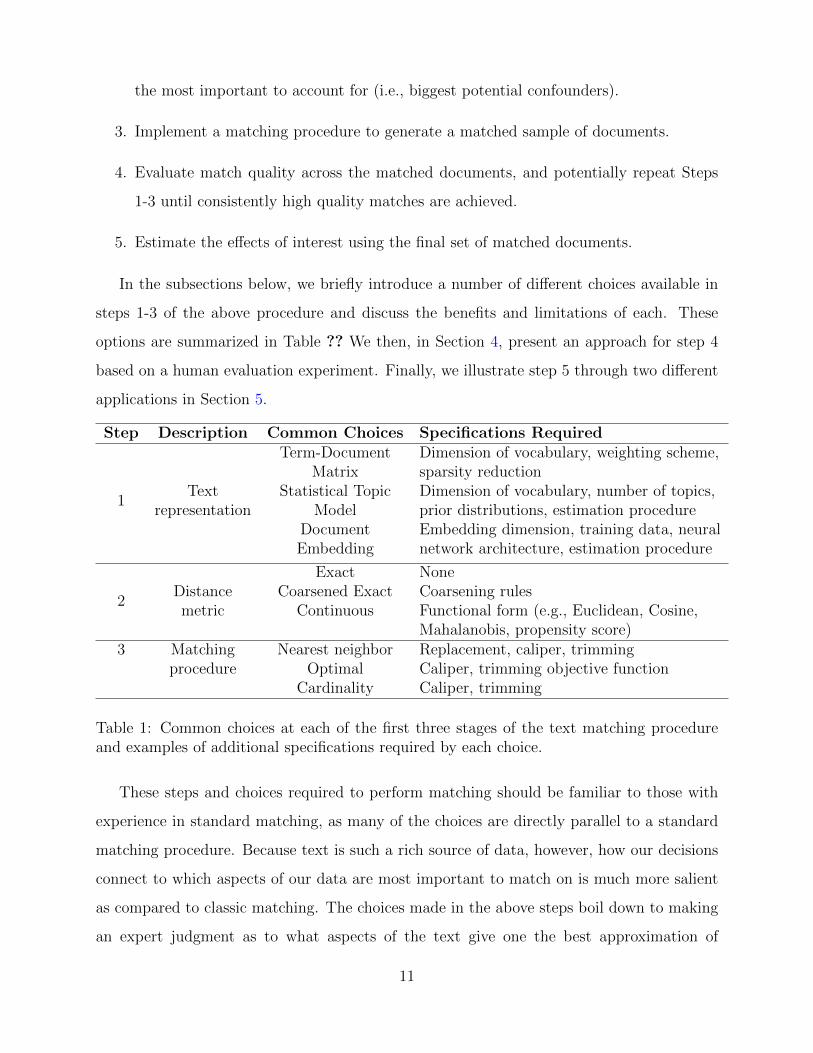
In the subsections below, we briefly introduce a number of different choices available in

steps 1-3 of the above procedure and discuss the benefits and limitations of each. These

options are summarized in Table ?? We then, in Section 4, present an approach for step 4

based on a human evaluation experiment. Finally, we illustrate step 5 through two different

applications in Section 5.

Step Description Common Choices Specifications Required

1

Term-Document Dimension of vocabulary, weighting scheme,Matrix sparsity reduction

Text Statistical Topic Dimension of vocabulary, number of topics,representation Model prior distributions, estimation procedure

Document Embedding dimension, training data, neuralEmbedding network architecture, estimation procedure

2

Exact NoneDistance Coarsened Exact Coarsening rulesmetric Continuous Functional form (e.g., Euclidean, Cosine,

Mahalanobis, propensity score)3 Matching Nearest neighbor Replacement, caliper, trimming

procedure Optimal Caliper, trimming objective functionCardinality Caliper, trimming

Table 1: Common choices at each of the first three stages of the text matching procedureand examples of additional specifications required by each choice.

These steps and choices required to perform matching should be familiar to those with

experience in standard matching, as many of the choices are directly parallel to a standard

matching procedure. Because text is such a rich source of data, however, how our decisions

connect to which aspects of our data are most important to match on is much more salient

as compared to classic matching. The choices made in the above steps boil down to making

an expert judgment as to what aspects of the text give one the best approximation of

11

selection on observables. In our media example, to illustrate, we judged that matching on

the story covered was the most important thing and therefore generated a human evaluation

experiment that targeted this particular measure and selected the procedure that performed

this task the best. For a more thorough discussion and description of the various choices

within these steps, see Appendix A.

3.1 Text representations

The representation of a text document transforms an ordered list of words and punctuation

into a vector of covariates, and is the most novel necessary component of matching with

text. To choose a representation, the researcher must first formulate a definition for textual

similarity that is appropriate for the study at hand. In some cases, all of the information

about potential confounders captured within the text data may be either directly estimable

(e.g., frequency of a particular keyword) or may be plausible to estimate using a single

numerical summary (e.g., the primary topic of a document estimated using a topic model).

In other cases, such a direct approach may not be possible.

The most common general representation of text is as a “bag-of-words,” containing uni-

grams and often bigrams, collated into a term-document matrix (TDM); the TDM may also

be rescaled according to Term Frequency-Inverse Document Frequency (TF-IDF) weighting.

Without additional processing, however, these vectors are typically very long; more parsi-

monious representations involve calculating a document’s factor loadings from unsupervised

learning methods like factor analysis or Structural Topic Models (STM) (Roberts et al.,

2016), or calculating a scalar propensity score for each document using the bag-of-words

representation (Taddy, 2013). Finally, we also consider a Word2Vec representation (Mikolov

et al., 2013), in which a neural network embeds words in a lower-dimensional space and a

document’s value is the weighted average of its words.

Each of these methods involves a number of tuning parameters. When using the bag-of-

words representation, researchers often remove very common and very rare words at arbitrary

thresholds, as these add little predictive power, or choose to weight terms by their inverse

document frequency; these pre-processing decisions can be very important (Denny and Spir-

ling, 2018). Topic models such as the STM are similarly sensitive to these pre-processing

12

decisions (Fan et al., 2017) and also require specification of the number of topics and select-

ing covariates, which are often unstable. Word2vec values depend on the dimensionality of

the word vectors as well as the training data and the architecture of the neural network.

Overall, when choosing a representation, researchers need to consider what aspects of the

text are confounding the outcome. For example, in our evaluation study that used matched

pairs of news articles from Fox News and CNN, we were interested in identifying pairs of

stories that were about the same general topic (e.g., plane crashes versus public policy) and

that also utilized the same set of keywords (e.g., “AirAsia” or “Obama”); this may suggest (as

we found) that representations that preserve the details of different keywords was important

for obtaining good matches. Generally, when the objective is to identify exact or nearly

exact matches, we recommend using text representations that retain as much information in

the text as possible. In particular, documents that are matched using the entire term-vector

will typically be similar with regards to both topical content and usage of keywords, while

documents matched using topic proportions may only be topically similar.

When the aspects of text are more targeted or specific, simply directly computing the

relevant covariates constructed by hand-coded rules may be the best option. That being said,

one might imagine that generally matching on the content of the text—as represented by the

specific words and phrases used—will frequently capture much of what different researchers

in different contexts may view as the necessary component for their selection on observables

assumption. Clearly this is an area for future work; as we see more matching with text in

the social sciences, we will also see a clear picture as to what structural aspects of text are

connected to the substantive aspects of text that researchers find important.

3.2 Distance metrics

Having converted the corpus into covariate representations, the second challenge is in com-

paring any two documents under the chosen representation to produce a measure of distance.

The two main categories of distance metrics are exact (or coarsened exact) distances, and

continuous distances. Exact distances consider whether or not the documents are identical

in their representation. If so, the documents are a match. Coarsened exact distance bins

each variable in the representation, then identifies pairs of documents which share the same

13

bins. If the representation in question is based on a TDM, these methods are likely to find

only a small number of high quality matches, given the large number of covariates that all

need to agree either exactly or within a bin. The alternative to exact distance metrics is

continuous distance metrics such as Euclidean distance, Mahalanobis distance, and cosine

distance. Counter to exact and coarsened exact metrics, which identify matches directly,

these metrics produce scalar values capturing the similarity between two documents.

3.3 Matching procedures

After choosing a representation and a distance metric, the choice of matching procedure often

follows naturally, as is the case in standard matching analyses. Exact and coarsened exact

distance metrics provide their own matching procedure, while continuous distance metrics

require both a distance formula and a caliper for specifying the maximum allowable distance

at which two documents may be said to still match. The calipers may be at odds with

the desired number of matches, as some treated units may have no control units within the

chosen caliper, and may subsequently be “pruned” by many common matching procedures.

Alternatively, researchers may allow any one treated unit to match multiple controls, or may

choose a greedy matching algorithm.

4 Experimental evaluation of text matching methods

In the previous section, we presented different forms of representations for text data and

described a number of different metrics for defining distance using each type of representation.

Any combination of these options could be used to perform matching. However, the quantity

and quality of matches obtained depend heavily on the chosen representation and distance

metric. For example, using a small caliper might lead to only a small number of nearly-exact

matches, while a larger caliper might identify more matches at the expense of overall match

quality. Alternatively, if CEM on a STM-based representation produces a large number

of low-quality matches, applying the same procedure on a TDM-based representation may

produce a smaller number of matches with more apparent similarities.

We investigate how this quantity versus quality trade-off manifests across different com-

14

binations of methods through an evaluation experiment performed with human subjects.

Applying several variants of the matching procedure described in Section 3 to a common

corpus, we explore how the quantity of matched pairs produced varies with different specifi-

cations of the representation and distance metric. Then, to evaluate how these choices affect

the quality of matched pairs, we rely on evaluations of human coders.

In this study, we consider five distance metrics (Euclidean distance, Mahalanobis distance,

cosine distance, distance in estimated propensity score, and coarsened exact distance), as

well as 26 unique representations,4 including nine different TDM-based representations, 12

different STM-based representations, and five Word2Vec embedding-based representations.

Crossing these two factors produces 130 combinations, where each combination corresponds

to a unique specification of the matching procedure described in Section 3. Among these

combinations, 5 specifications are variants of the TIRM procedure developed in Roberts

et al. (2018). Specifications of each of the procedures are provided in Appendix B.

To compare the different choices of representation and distance metric considered here,

we apply each combination to a common corpus to produce a set of matched pairs for each.

We use a corpus of N = 3, 361 news articles published from January 20, 2014 to May

9, 2015, representing the daily front matter content for each of two online news sources:

Fox News (N = 1, 796) and CNN (N = 1, 565). The news source labels were used as the

treatment indicator, with Z = 1 for articles published by Fox News and Z = 0 for articles

published by CNN. To match, we first calculate the distances between all possible pairs of

treated and control units based on the specified representation and distance metric. Each

treated unit is then matched to a set of control units with whom its distance was within the

specified caliper.5 Using this procedure, 13 of the original 130 specifications considered did

not identify any matched pairs. The union of matched pairs identified across the remaining

4Because estimation and distance calculations with high-dimensional text representations can be com-putationally intensive, we restrict our analyses to this set of 26 possible representations, which we believeprovide an adequate representation of the spectrum of possible text-representations that could be used forapplications of text-matching. However, we emphasize that the methods presented in this paper, includingthe procedure for text-matching and the framework for performing systematic evaluations of text-matchingmethods, can be extended to include any number of additional variants to the representations consideredhere.

5For each of the combinations that did not use the CEM metric, the caliper was calculated as the 0.1thquantile of the distribution of distances under that combination for all 1796 × 1565 = 2,810,740 possiblepairs of articles.

15

117 procedures resulted in 30,647 unique pairs.

Each procedure identified between 41 and 1605 total pairs of matched articles, with an

average of 502 pairs produced per matching procedure. These pairs covered between 69 to

2942 unique articles within the corpus. Specifically, each procedure identified one or more

matches for between 34 (2%) and 1566 (87%) of the 1796 unique articles published by Fox

News and identified matches for between 20 (1%) and 1376 (88%) of the 1565 unique CNN

articles.

Conversely, each of the 30,647 unique pairs of matched articles was identified, on average,

by 1.91 of the 117 different procedures, with 6,910 (22.5%) of unique pairs matched by

between 2 to 55 of the 117 procedures and the remaining 23,737 pairs matched by only one

procedure. We view the frequency of each unique pair within the sample of 58,737 pairs

identified as a rough proxy for match quality because, ideally when performing matching,

the final sample of matched pairs identified will be robust to different choices of the distance

metric or representation. Thus, we expect that matched pairs that are identified by multiple

procedures will have higher subjective match quality than singleton pairs.

4.1 Measuring match quality

In standard applications of matching, if two units that are matched do not appear substan-

tively similar, then any observed differences in outcomes may be due to poor match quality

rather than the effect of treatment. Usual best practice is to calculate overall balance between

the treatment and control groups, which is typically measured by the difference-in-means

for all covariates of interest. If differences on all matched covariates are small in magnitude,

then the samples are considered balanced, and thus, typically, well-matched.

As previously discussed, to calculate balance in settings where the covariates are text

data, these standard balance measures typically fail to capture meaningful differences in the

text. Further, due to the curse of dimensionality in these settings, it is likely that at least

some (and probably many) covariates will be unbalanced between treatment and control

groups. Thus, to measure match quality we rely on a useful property of text: its ease of

interpretability. A researcher evaluating two units that have been matched on demographic

covariates, for example, may be unable to verify the quality of a matched pair. However,

16

depending on what aspects of text the researcher is substantively attempting to match on,

human coders who are tasked with reading two matched text documents are often amply

capable of quantifying their subjective similarity if given instructions as to what to attend

to. We leverage this property to measure match quality using an online survey of human

respondents, where match quality is defined on a scale of 0 (lowest quality) to 10 (highest

quality).

To obtain match quality ratings, we conducted a survey experiment using Amazon’s

Mechanical Turk (MTurk) and the Digital Laboratory for the Social Sciences (DLABSS)

(Enos et al., 2016). Online crowd-sourcing platforms such as these have been shown to

be effective for similarity evaluations in a number of settings (Mason and Suri, 2012). For

instance, a study by Snow et al. (2008) that tasked non-expert human workers on MTurk

with five natural language evaluations reported a high degree of agreement between the

crowd-sourced results and gold-standard results provided by experts. In the present study,

respondents were first informed about the nature of the task and then given training6 on

how to evaluate the similarity of two documents. After completing training, participants

were then presented with a series of 11 paired newspaper articles, including an attention

check and an anchoring question, and asked to assign a similarity rating. For each question,

participants were instructed to read both articles in the pair and rate the articles’ similarity

from zero to ten, where zero indicates that the articles are entirely unrelated and ten indicates

that the articles are covering the exact same event. Snapshots of the survey are presented

in Appendix C.

We might be concerned that an online convenience sample may not be an ideal population

for conducting this analysis, and that their perceptions of article similarity might differ from

the overall population, or from trained experts. To assess the reliability of this survey as

an instrument for measuring document similarity, we leverage the fact that we performed

two identical pilot surveys prior to the experiment using respondents from two distinct

6For training, participants were first informed about the nature of the task. Next, participants werepresented with a scoring rubric and were informed to use this rubric as “a guide to help [them] determinethe similarity of a pair of articles.” In the final component of training, participants were asked to read andscore three pre-selected pairs of articles, which were chosen to represent pairings that we believe have matchquality scores of zero, five, and ten, respectively. After scoring each training pair, participants were informedabout the anticipated score for that pair and provided with an explanation for how that determination wasmade.

17

populations and found a high correlation (ρ = 0.85) between the average match quality

scores obtained from each sample. Additional details about this assessment are provided

in Appendix D. We take note that these populations, MTurkers and DLABSS respondents,

are both regularly used as coders to build training data sets for certain tasks in machine

learning; the hallmark of these tasks is that they are easily and accurately performed by

untrained human respondents. We argue that this task of identifying whether two articles

discuss related stories falls squarely in this category, and our inter-coder reliability test in

Appendix D supports this argument.7

In an ideal setting, for each unique matched pair identified using the procedure described

above, we would obtain a sample of similarity ratings from multiple human coders. Aggre-

gating these ratings across all pairs in a particular matched data set would then allow us to

estimate the average match quality corresponding to each of the 130 procedures considered,

with the quality scores for the 13 procedures that identified no matches set to zero. Though

this is possible in principle, to generate a single rating for each unique matched pair requires

that a human coder read both documents and evaluate the overall similarity of the two ar-

ticles. This can be an expensive and time-consuming task. Thus, in this study, it was not

possible to obtain a sample of ratings for each of the 30,647 unique pairs.

Instead, we took a stratified, weighted sample of pairs such that the resulting sample

would be representative of the population of all 30,647 unique matched pairs as well as the

population of 2,780,093 pairs of documents that were not identified by any of the matching

procedures. Specifically, the sample was chosen such that each of the 130 matching proce-

dures that identified a non-zero number of matches would be represented by at least four

pairs in the experiment. For each stratum, the sampling weights for each pair were calcu-

lated proportional to the estimated match quality of that pair, calculated using a predictive

model trained on human-coded data from a pilot experiment. We also sampled an additional

50 unique pairs from the pool of 2,780,093 pairs not identified by any matching procedures.

Ratings obtained from these pairs can be used to obtain a reference point for interpreting

match quality scores. The resulting sample consisted of 505 unique pairs ranging the full

7For researchers interested in conducting their own text matching evaluation studies, we note that MTurkand DLABSS populations may not always be applicable, especially in contexts where domain expertise isrequired.

18

spectrum of predicted match quality scores. Each respondent’s set of nine randomly selected

questions were drawn independently such that each pair would be evaluated by multiple

respondents. Using this scheme, each of the 505 sampled pairs was evaluated by between

six and eleven different participants (average of 9). Question order was randomized, but the

anchor was always the first question, and the attention check was always the fifth question.

We surveyed a total of 505 respondents. After removing responses from 52 participants

who failed the attention check,8 all remaining ratings were used to calculate the average

match quality for each of the 505 sampled pairs evaluated. These scores were then used

to evaluate each of the 130 combinations of methods considered in the evaluation, where

the contribution of each sampled pair to the overall measure of quality for a particular

combination of methods was weighted according to its sampling weight. This inferential

procedure is described more formally in Appendix E.

4.2 Results

4.2.1 Which automated measures are most predictive of human judgment about

match quality?

Our primary research question concerns how unique combinations of text representation and

distance metric contribute to the quantity and quality of obtained matches in the interest

of identifying an optimal combination of these choices in a given setting. We can estimate

the quality of the 130 matching methods considered in the evaluation experiment using

weighted averages of the scores across the 505 pairs evaluated by human coders. However, it

is also of general interest to be able to evaluate new matching procedures without requiring

additional human experimentation. We also want to maximize the precision of our quality

estimates for the 130 methods considered in this study. To these ends, we examine if we

can predict human judgment about match quality based on the distance scores generated by

each different combination of one representation and one distance metric. If the relationship

between the calculated match distance and validated match quality is strong, then we may

8The attention check consisted of two articles with very similar headlines but completely different articletext. The text of one article stated that this question was an attention check, and that the respondentshould choose a score of zero. Participants who did not assign a score of zero on this question are regardedas having failed the attention check.

19

be confident that closely-matched documents, as rated under that metric, would pass a

human-subjects validation study.

To evaluate the influence of each distance score on match quality, we take the pairwise

distances between documents for each of the 505 matched pairs used in the evaluation ex-

periment under different combinations of the representations and distance metrics described

in Section 3. After excluding all CEM-based matching procedures, under which all pairwise

distances are equal to zero or infinity by construction, all distances were combined into a

data set containing 104 distance values for each of the 505 matched pairs. Figure 1 gives

six examples of how these distances correlate with observed match quality based on human

ratings of similarity, along with the fitted regression line obtained from quadratic regressions

of average match quality on distance. Here, the strong correlations suggest that automated

measures of match quality could be useful for predicting human judgment. The particularly

strong relationship between the cosine distance metric calculated over a TDM-based repre-

sentation provides additional evidence in favor of matching using this particular combination

of methods. These findings also suggest that the increased efficiency achieved with TDM

cosine matching is not attributable to the cosine distance metric alone, since the predictive

power achieved using cosine distance on a Word2Vec (W2V) representation or a STM-based

representation is considerably lower than that based on a TDM-based representation.

To leverage the aggregate relationship of the various machine measures of similarity on

match quality, we developed a model for predicting the quality of a matched pair of docu-

ments based on the 104 distance scores, which we then trained on the 505 pairs evaluated in

our survey experiment. For estimation, we use the LASSO (Tibshirani, 1996), implemented

with ten-fold cross validation (Kohavi et al., 1995). Here, for each of the 505 pairs, the

outcome was defined as the average of the ratings received for that pair across the human

coders, and the covariates were the 104 distance measures. We also included quadratic terms

in the model, resulting in a total of p=208 terms. Of these, the final model obtained from

cross-validation selected 19 terms with non-zero coefficients. However, our results suggest

that the majority of the predictive power of this model primarily comes from two terms:

cosine distance over the full, unweighted term-document matrix and cosine distance over an

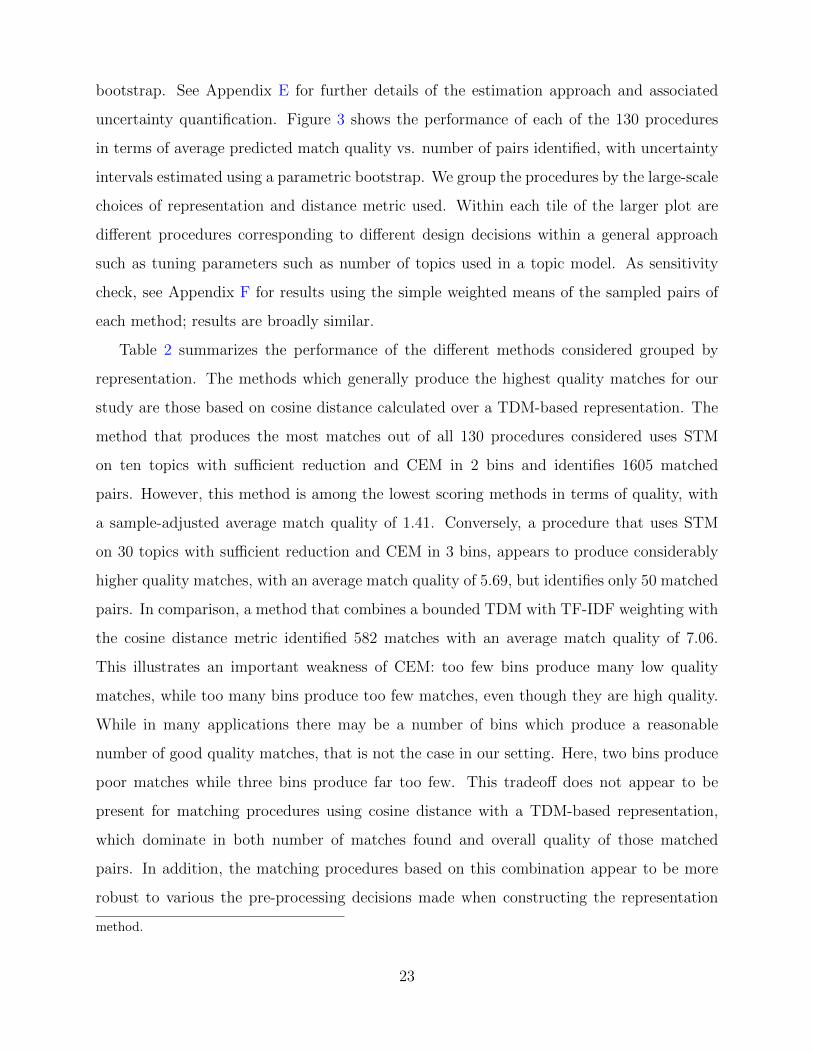
STM with 100 topics. Figure 2 shows the out-of-sample predictive performance of the model

20

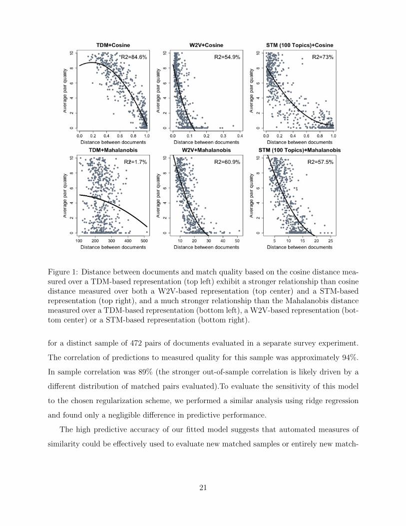
Figure 1: Distance between documents and match quality based on the cosine distance mea-sured over a TDM-based representation (top left) exhibit a stronger relationship than cosinedistance measured over both a W2V-based representation (top center) and a STM-basedrepresentation (top right), and a much stronger relationship than the Mahalanobis distancemeasured over a TDM-based representation (bottom left), a W2V-based representation (bot-tom center) or a STM-based representation (bottom right).

for a distinct sample of 472 pairs of documents evaluated in a separate survey experiment.

The correlation of predictions to measured quality for this sample was approximately 94%.

In sample correlation was 89% (the stronger out-of-sample correlation is likely driven by a

different distribution of matched pairs evaluated).To evaluate the sensitivity of this model

to the chosen regularization scheme, we performed a similar analysis using ridge regression

and found only a negligible difference in predictive performance.

The high predictive accuracy of our fitted model suggests that automated measures of

similarity could be effectively used to evaluate new matched samples or entirely new match-

21

Figure 2: Predictive model for match quality trained on human evaluations has a correlationof 0.944 with observed quality scores obtained in a separate human evaluation experimenton a different set of pairs, indicating high out-of-sample predictive accuracy.

ing procedures without requiring any additional human evaluation.9 We can also use it

to enhance the precision of our estimates of match quality for the 130 matching methods

considered in the evaluation experiment using model-assisted survey sampling methods.

4.2.2 Which methods make the best matching procedures?

To compare the performance of the final set of 130 matching procedures considered in our

study, we, for each method, estimate the average quality of all pairs selected by that method.

We increase precision of these estimates using model-assisted survey sampling. In particular,

we first use the predictive model described above to predict the quality of all matched pairs

of a method. This average quality estimate is then adjusted by a weighted average of the

residual differences between predicted and actual measured quality for those pairs directly

evaluated in the human experiment. (The average quality scores for the 13 procedures that

identified no matches are all set equal to zero.) This two-step process does not depend on

the model validity and is unbiased.10 We assess uncertainty with a variant of the parametric

9Since this model was trained on human evaluations of matched newspaper articles, extrapolating pre-dictions may only be appropriate in settings with similar types of documents. However, our experimentalframework for measuring match quality could be implemented using text data to build a similar predictivemodel in other contexts.

10Nearly unbiased that is. There is a small bias term due using a Hajek-style approach rather than Horvitz-Thompson. This comes from the sample having a random total weight due to using the weighted sampling

22

bootstrap. See Appendix E for further details of the estimation approach and associated

uncertainty quantification. Figure 3 shows the performance of each of the 130 procedures

in terms of average predicted match quality vs. number of pairs identified, with uncertainty

intervals estimated using a parametric bootstrap. We group the procedures by the large-scale

choices of representation and distance metric used. Within each tile of the larger plot are

different procedures corresponding to different design decisions within a general approach

such as tuning parameters such as number of topics used in a topic model. As sensitivity

check, see Appendix F for results using the simple weighted means of the sampled pairs of

each method; results are broadly similar.

Table 2 summarizes the performance of the different methods considered grouped by

representation. The methods which generally produce the highest quality matches for our

study are those based on cosine distance calculated over a TDM-based representation. The

method that produces the most matches out of all 130 procedures considered uses STM

on ten topics with sufficient reduction and CEM in 2 bins and identifies 1605 matched

pairs. However, this method is among the lowest scoring methods in terms of quality, with

a sample-adjusted average match quality of 1.41. Conversely, a procedure that uses STM

on 30 topics with sufficient reduction and CEM in 3 bins, appears to produce considerably

higher quality matches, with an average match quality of 5.69, but identifies only 50 matched

pairs. In comparison, a method that combines a bounded TDM with TF-IDF weighting with

the cosine distance metric identified 582 matches with an average match quality of 7.06.

This illustrates an important weakness of CEM: too few bins produce many low quality

matches, while too many bins produce too few matches, even though they are high quality.

While in many applications there may be a number of bins which produce a reasonable

number of good quality matches, that is not the case in our setting. Here, two bins produce

poor matches while three bins produce far too few. This tradeoff does not appear to be

present for matching procedures using cosine distance with a TDM-based representation,

which dominate in both number of matches found and overall quality of those matched

pairs. In addition, the matching procedures based on this combination appear to be more

robust to various the pre-processing decisions made when constructing the representation

method.

23

Figure 3: Number of matches found versus average model-assisted match quality scores foreach combination of matching methods. Grey points indicate procedures with extreme reduc-tion in information (e.g., procedures that match on only stop words). Blue circles highlightprocedures that use existing state-of-the-art methods for text matching. One procedure withmany low quality pairs at coordinates (1605,1.39) is excluded from this plot.

than procedures that use an alternative distance metric or representation, as illustrated by

the tight clustering of the variants of this general approach on the plot.

Overall, our results indicate that, in our context, matching on the full TDM produces

both more and higher quality matches than matching on a vector of STM loadings when

considering the content similarity of pairs of news articles. Moreover, TDM-based represen-

tations with cosine matching appear relatively robust to tuning parameters including the

degree of bounding applied and the choice of weighting scheme. STM-based representations,

on the other hand, appear to be somewhat sensitive to tuning parameters, with represen-

tations that include a large number of topics achieving higher average match quality than

24

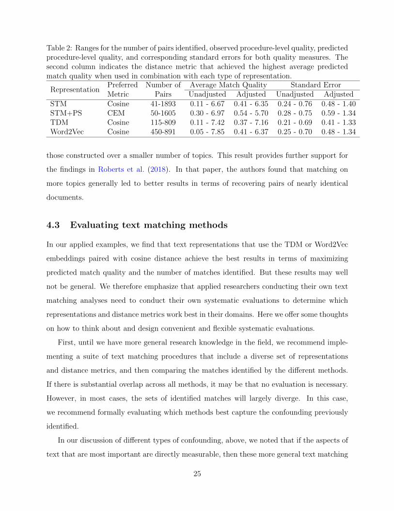
Table 2: Ranges for the number of pairs identified, observed procedure-level quality, predictedprocedure-level quality, and corresponding standard errors for both quality measures. Thesecond column indicates the distance metric that achieved the highest average predictedmatch quality when used in combination with each type of representation.

RepresentationPreferred Number of Average Match Quality Standard ErrorMetric Pairs Unadjusted Adjusted Unadjusted Adjusted

STM Cosine 41-1893 0.11 - 6.67 0.41 - 6.35 0.24 - 0.76 0.48 - 1.40STM+PS CEM 50-1605 0.30 - 6.97 0.54 - 5.70 0.28 - 0.75 0.59 - 1.34TDM Cosine 115-809 0.11 - 7.42 0.37 - 7.16 0.21 - 0.69 0.41 - 1.33Word2Vec Cosine 450-891 0.05 - 7.85 0.41 - 6.37 0.25 - 0.70 0.48 - 1.34

those constructed over a smaller number of topics. This result provides further support for

the findings in Roberts et al. (2018). In that paper, the authors found that matching on

more topics generally led to better results in terms of recovering pairs of nearly identical

documents.

4.3 Evaluating text matching methods

In our applied examples, we find that text representations that use the TDM or Word2Vec

embeddings paired with cosine distance achieve the best results in terms of maximizing

predicted match quality and the number of matches identified. But these results may well

not be general. We therefore emphasize that applied researchers conducting their own text

matching analyses need to conduct their own systematic evaluations to determine which

representations and distance metrics work best in their domains. Here we offer some thoughts

on how to think about and design convenient and flexible systematic evaluations.

First, until we have more general research knowledge in the field, we recommend imple-

menting a suite of text matching procedures that include a diverse set of representations

and distance metrics, and then comparing the matches identified by the different methods.

If there is substantial overlap across all methods, it may be that no evaluation is necessary.

However, in most cases, the sets of identified matches will largely diverge. In this case,

we recommend formally evaluating which methods best capture the confounding previously

identified.

In our discussion of different types of confounding, above, we noted that if the aspects of

text that are most important are directly measurable, then these more general text matching

25

approaches are not needed, strictly speaking. In this case we recommend directly assessing

balance on specific covariates built from the text. But if general text matching methods are

used in such contexts, we believe checking these core covariates to still be of use as signals

as to which methods are at least achieving balance on some core summary statistics. This

is akin to viewing mean balance as a proxy for covariate balance in classic matching.

If the potential confounding truly hinges on the more complex and latent aspects of

text, however, then one could ideally leverage human judgment to hand evaluate the full

set of possible matched pairs of text documents. In our case, for example, we could, given

unlimited resources, ask human coders to read through the entire corpus of news articles

and put them into bins according to which stories they cover. Even untrained human coders

could be reliably good at this task. This, of course, is generally not possible, but we hope

the methods described above serve a similar function.

As we have seen, we can evaluate the success of such an attempt by inverting the full

human-coding procedure to generate a test: we identify a set of possible matches using

automated text matching methods and then and present a subset of them to trained human

coders. These human coders can then evaluate sample pairs of matched documents to

determine which matches are systematically “best” according to their own judgment. Using

this information we can then see which methods appear to best match on the targeted aspects

of text. This human coding task is of utmost importance, requiring both careful pretesting

and substantial guidance to ensure the humans attend to the aspects of text deemed most

important as potential confounders. In particular, the primary concern is instructing the

human coders to evaluate similarity along the latent dimension of interest, which in our

media case is whether any two articles truly cover the same events or issues.

One final circumstance bears discussion: it may be the case that the identified latent

dimension of interest is challenging or impossible for human evaluators to reliably code. For

example, even two experienced medical doctors may systematically disagree in their readings

of patient data such as X-rays (Steiner et al., 2018). In such cases, human evaluations may

not serve as a reliable ground truth to which automated text match quality may be compared.

It is still possible that automated text matching methods would work well in these cases,

but researchers cannot validate those results in this framework.

26

This and other open questions, including identifying what contexts would have topic

model- or propensity score-based representations outperform TDM-based or Word2Vec embedding-

based representations, we leave to future research.

5 Applications

5.1 Decomposing media bias

While American pundits and political figures continue to accuse major media organizations

of “liberal bias,” scholars, after nearly two decades of research on the issue, have yet to come

to a consensus about how to measure bias, let alone determine its direction. A fundamental

challenge in this domain is how to disentangle the component of bias relating to how a story

is covered, often referred to as “presentation bias” (Groseclose and Milyo, 2005; Gentzkow

and Shapiro, 2006; Ho et al., 2008; Gentzkow and Shapiro, 2010; Groeling, 2013), from

the component relating to what is covered, also known as “selection bias” (Groeling, 2013)

or “topic selection.” In particular, systematic comparisons of how stories are covered by

different news sources (e.g., comparing the level of positive sentiment expressed in the article)

may be biased by differences in the content being compared. We present a new approach for

addressing this issue by using text matching to control for selection bias.

We analyze a corpus consisting of N = 9, 905 articles published during 2013 by each

of 1311 popular online news outlets. This data was collected and analyzed in Budak et al.

(2016). The news sources analyzed here consist of Breitbart, CNN, Daily Kos, Fox News,

Huffington Post, The Los Angeles TImes, NBC News, The New York Times, Reuters, USA

Today, The Wall Street Journal, The Washington Post, and Yahoo. In addition to the text

of each article, the data include labels indicating each articles’ primary and secondary topics,

where these topics were chosen from a set of 15 possible topics by human coders in a separate

evaluation experiment performed by Budak et al. (2016). The data also include two human-

coded outcomes that measure the ideological position of each article on a 5-point Likert scale.

Specifically, human workers tasked with reading and evaluating the articles were asked “on

11The original data included 15 news sources, but BBC and The Chicago Tribune are excluded from thisanalysis due to insufficient sample sizes for these sources

27

a scale of 1-5, how much does this article favor the Republican party?”, and similarly, “on a

scale of 1-5, how much does this article favor the Democratic party?”

To perform matching on this data, we use the optimal procedure for identifying articles

covering the same underlying story identified by our prior evaluation experiment: cosine

matching on a bounded TDM.12 Because in this example we have a multi-valued treatment

with 13 levels, each representing a different news source, we follow the procedure for template

matching13 described in Silber et al. (2014) to obtain matched samples of 150 articles across

all treatment groups. In brief, the template matching procedure first finds a representative

set of stories across the entire corpus, and uses that template to find a sample of similar

articles within each source that collectively cover this canonical set of topics. This allows

us to identify a set of articles sampled from each source that are all similar to the same

template and therefore similar to each other.

Before matching, our estimates of a news source’s average favorability are a measure of

overall bias, which includes biases imposed through differential selection of content to publish

as well as biases imposed through the language and specific terms used when covering the

same content. The matching controls selection biases due to some sources selecting different

stories that may be more or less favorable to a given party than other stories. Differences

in estimated favorability on the matched articles can be attributed to presentation bias.

The difference between estimates of average favorability before matching (overall bias) and

estimates after matching (presentation bias) therefore represent the magnitude of selection

biases imposed by the sources. Large differences between pre- and post-matched estimates

indicate a stronger influence of selection bias relative to presentation bias.

Figure 4 shows the average favorability toward Democrats (blue) and Republicans (red)

for each news source overall, and the average favorability among the template matched

12Since the outcomes of interest in this analysis are human-coded measures of favorability toward democratsand republicans, we limit the vocabulary of the TDM to include only nouns and verbs to avoid matching onaspects of language that may be highly correlated with these outcomes.

13To implement the template matching procedure, we first generate a template sample of N = 150 articleschosen to be the most representative of the corpus in terms of the distribution of primary topics among 500candidate samples of this size. Once this template is chosen, for each treatment level (i.e., news source),we then perform optimal pair matching within primary topics to identify a sample of 150 articles from thatsource that most closely match the template sample with regards to cosine distance calculated over the TDM.Iterating through each of the 13 target sources, this produces a final matched sample of 13 × 150 = 1, 950matched articles.

28

Figure 4: Estimates of average favorability toward Democrats (blue) and Republicans (red)for each source both before and after matching.

documents. Arrows begin at the average score before matching, and terminate at the average

score after matching. The length of the arrows is the estimated magnitude of the bias of

each source that is attributable to differences in selection.

Before discussing the pattern of shifts, we first look at overall trends of favorability

across sources. First, overall sentiment towards Republicans generally hovers around 2.8 to

3.1, slightly less, on average, than the partisan neutrality of x = 3, which corresponds to a

response of “neither favorable nor unfavorable.” The one exception is the Daily Kos, which

is unfavorable. Other sources (CNN, the Huffington Post, the NY Times, and the LA Times)

are at the low end of this range, indicating some negative sentiment. For the Democrats,

there is somewhat more variation, however, with Brietbart being the least favorable, followed

by Fox and WSJ, and the Daily Kos being the most.

Furthermore, it is primarily the more extreme sources that show selection effects. Bre-

29

itbart, Fox and WSJ, for example, all become more positive towards Democrats and less

positive towards Republicans when we adjust for story. This suggests they tend to select

stories that are biased more towards Republicans and away from Democrats, a selection bias

effect. Similarly, the LA Times and Daily Kos show the opposite trends, again showing selec-

tion bias effects in the opposite direction. The remaining sources do not appear significantly

be impacted by controlling for selection.

We performed a series of sensitivity checks to assess the stability of our results to different

specifications of the matching procedure and/or different choices of template sample. We also

examine the variability due to randomly matching documents to assess how much estimation

uncertainty is present in our analysis. Details of these analyses are provided in Appendix

G. Generally, we see that estimating the selection effect of an individual source is difficult,

and that the magnitude of the selection effects tends to be small, indicating that the choice

of what stories to cover is not driving the overall favorability ratings. In other words, most

differences in favorability appear to be driven by presentation bias.

5.2 Improving covariate balance in observational studies

In our second application, we demonstrate how text matching can be used to strengthen

inferences in observational studies with text data. Specifically, we show that text matching

can be used to control for confounders measured by features of the text that would otherwise

be missed using traditional matching schemes.

We use a subset of the data first presented in Feng et al. (2018), which conducted an ob-

servational study designed to investigate the causal impact of bedside transthoracic echocar-

diography (TTE), a tool used to create pictures of the heart, on the outcomes of adult

patients in critical care who are diagnosed with sepsis. The data were obtained from the

Medical Information Mart for Intensive Care (MIMIC) database (Johnson et al., 2016) on

2,401 patients diagnosed with sepsis in the medical and surgical intensive care units at a

Massachusetts Institute of Technology university hospital located in Boston, Massachusetts.

Within this sample, the treatment group consists of 1,228 patients who received a TTE

during their stay in the ICU (defined by time stamps corresponding to times of admission

and discharge) and the control group is comprised of 1,173 patients who did not receive a

30

TTE during this time. For each patient we observe a vector of pre-treatment covariates

including demographic data, lab measurements, and other clinical variables. In addition to

these numerical data, each patient is also associated with a text document containing intake

notes written by nursing staff at the time of ICU admission.14 The primary outcome in this

study was 28-day mortality from the time of ICU admission.

Because the treatment in this study was not randomly assigned to patients, it is possible

that patients in the treatment and control groups may differ systematically in ways that

affect both their assignment to treatment versus control and their 28-day mortality. For

instance, patients who are in critical condition when admitted into the ICU may die before

treatment with a TTE has been considered. Similarly, patients whose health conditions

quickly improve after admission may be just as quickly discharged. Therefore, in order to

obtain unbiased estimates of the effects of TTE on patient mortality, it is important to

identify and appropriately adjust for any potentially confounding variables such as degree of

health at the time of admission.

We apply two different matching approaches to this data: one that matches patients

only on numerical data and ignores the text data, and one that matches patients using both

the numerical and text data. In the first procedure, following Feng et al. (2018), we match

treated and control units using optimal one-to-one matching (Hansen and Klopfer, 2006) on

estimated propensity scores15. We enforce a propensity score caliper equal to 0.1 standard

deviations of the estimated distribution, which discards any treated units for whom the

nearest control unit is not within a suitable distance. In the second approach, we perform

optimal one-to-one text matching within propensity score calipers. Intuitively, this procedure

works by first, via the calipers, reducing the space of possible treated-control pairings in a way

that ensures adequate balance on numerical covariates. By then performing text matching

within this space to select a specific match given a set of candidate matches all within the

calipers, we obtain matched samples that are similar with respect to all observed covariates,

including the original observed covariates and any variables that were not recorded during

14For the purposes of this study, all text data were pre-processed to remove formatting, punctuation, andspelling errors. After pre-processing, the final corpus of N=2,401 documents contained a vocabulary of14,266 unique terms, with each document containing between two and 861 terms.

15Estimated propensity scores are calculated by fitting a logistic regression of the indicator for treatmentassignment (receipt of TTE) on the observed numerical covariates.

31

the study but can be estimated by summary measures of the text.

Identifying the optimal text-matching method here requires careful consideration of how

text similarity should be defined and evaluated in this medical context. Here, the ideal text-

matching method is one that matches documents on key medical concepts and prognostic

factors that could both impact choice of using TTE as well as the outcome (i.e., potential

confounders) that are captured within the text data. Unlike in the previous application,

these features cannot be reliably evaluated by non-expert human coders due to the domain

expertise and familiarity with medical jargon necessary to make comparisons between medical

documents. Thus, to perform a systematic evaluation of text matching methods in this study,

we adopt an information retrieval approach for comparing medical texts that has been widely

applied in the biomedical literature (Aronson, 2001; Zeng et al., 2007).

In particular, by consulting with medical professionals, we first obtained a mapping of

the texts to a set of clinically meaningful concepts that could be used to characterize ICU

patients. Following the approach of MacLean and Heer (2013), we then calculated the

Jaccard similarity over this mapping between matched pairs of documents as an omnibus

measure of match quality. We treat these scores as a working gold standard for this particular

application; these scores are based on careful consideration from domain experts who have

the medical background required to extract potentially confounding information from this

type of nuanced text. When such a mapping is available, the Jaccard similarity metric offers

a practical alternative to human evaluation for obtaining estimates of match quality that

can be used to compare the relative performance of different matching procedures. However,

this metric may not be appropriate for evaluating new texts or for measuring text similarity

in other contexts. Figure 5 shows the average pairwise Jaccard similarity achieved after

matching (within propensity score calipers based on the numerical covariates) using each of

the 130 text matching specifications described in Section 3. The best-performing procedure

matches each treated unit to its nearest control based on the cosine distance calculated over

a bounded16 TDM, where treated units whose nearest control is outside the specified caliper

are discarded.

16The best identified TDM is bounded to exclude extremely rare and extremely frequent terms, definedoperationally as terms that appear in less than four or more than 1000 documents within this corpus.

32

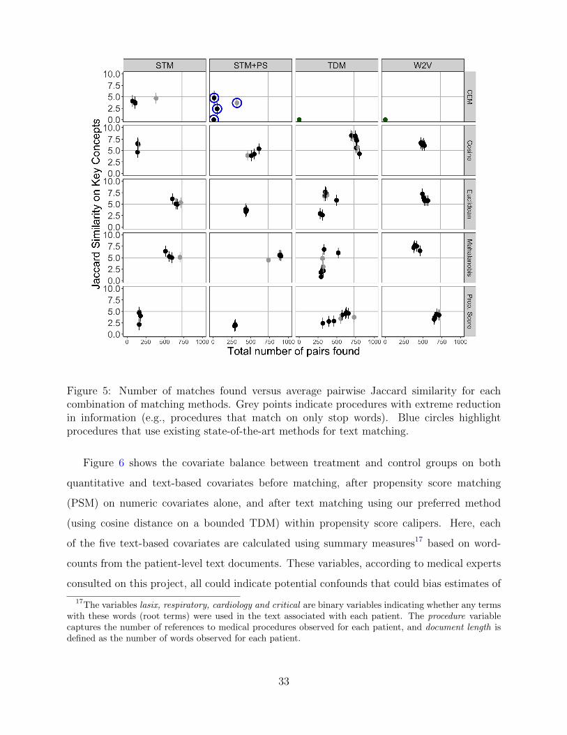
Figure 5: Number of matches found versus average pairwise Jaccard similarity for eachcombination of matching methods. Grey points indicate procedures with extreme reductionin information (e.g., procedures that match on only stop words). Blue circles highlightprocedures that use existing state-of-the-art methods for text matching.

Figure 6 shows the covariate balance between treatment and control groups on both

quantitative and text-based covariates before matching, after propensity score matching

(PSM) on numeric covariates alone, and after text matching using our preferred method

(using cosine distance on a bounded TDM) within propensity score calipers. Here, each

of the five text-based covariates are calculated using summary measures17 based on word-

counts from the patient-level text documents. These variables, according to medical experts

consulted on this project, all could indicate potential confounds that could bias estimates of

17The variables lasix, respiratory, cardiology and critical are binary variables indicating whether any termswith these words (root terms) were used in the text associated with each patient. The procedure variablecaptures the number of references to medical procedures observed for each patient, and document length isdefined as the number of words observed for each patient.

33

impact if not controlled. Our general text matching methods do not directly balance these

covariates; the improved balance is a consequence of matching on the more general overall

distance metric and representation used.

Figure 6: Standardized differences in means with 95% confidence intervals between treatmentand control groups on 26 numerical covariates and 5 text-based covariates (denoted by *)before matching (gray), after propensity score matching (red), and after text matching (blue).

Table 3: Survival rates for treatment and control groups and estimated treatment effectsbefore and after propensity score matching (PSM) and text matching within propensityscore calipers.

ProcedureEffective Survival Rate Difference

Sample Size Treatment Control (Std. Error)Before Matching 1186 72.5% 71.2% 1.3% (1.8%)

PSM 807 72.5% 67.7% 4.8% (2.2%)Text Matching 894 72.5% 67.5% 5.0% (2.1%)

34

In general, common wisdom (e.g., (Imbens and Rubin, 2015)) is to condition on all avail-

able data that could indicate potential confounding influences when making inferences using

observational data. While PSM is able to adequately balance the numerical covariates and

some of the text-based covariates most correlated with these numerical measures, it fails

to sufficiently adjust for differences between treatment and control groups on a number of

potential confounders captured only by the text. For instance, both the unmatched data

and the matched sample generated using PSM have large imbalances between treatment

and control groups on references to Lasix, a medication commonly used to treat congestive

heart failure. In the unmatched sample, only 10% of treated units have documents con-

taining references to this medication compared to 28% of control units who are associated

with the medication. Matching on the estimated propensity scores reduces this imbalance

only slightly, while cosine matching within propensity score calipers shows a considerable

improvement in the balance achieved between treatment groups on this variable. Incorpo-

rating the text data into the matching procedure leads to similar improvements in balance

for the other five text-based variables while also maintaining suitable overall balance on the

numerical covariates.

Table 3 summarizes the survival rates in the treatment and control groups within each

matched sample along with the effective sample sizes (i.e., the equivalent number of matched

pairs) in the final matched samples. Generally, there appears to be some confounding, with

the adjusted impacts being larger than the naıve differences. The matched sample identified

using text matching is slightly larger in terms of effective sample size than simple PSM,

although they are not significantly different. This increase in effective sample size highlights

the efficiency of text matching; when evaluating multiple control units that are eligible

matches for a single treated unit in terms of quantitative covariates, the text-based distance

offers a more refined measure of pairwise similarity than distances based on the propensity

score. Further, when text matching within propensity score calipers, small differences in

estimated propensity scores across control units will be offset by any large differences in

text. In the present application, this allows for more precise and efficient optimization of the

matched sample.

Of course, conducting a matched analysis is rooted in thoughtful design. In particular,

35

the researcher must decide which variables are important potential confounders, and which

are not. This is especially important when balancing the trade-offs between achieving better

balance on some variables at the expense of others. The purpose of highlighting text matching

in this context is to demonstrate how information from the text can also be included in

these decisions of what to attend to. If the text is deemed not informative, then of course

it should not be an important consideration with matching. But, as in this case, if the text

is considered to indicate significant aspects of patient condition that should be attended to,

the general matching procedures we have discussed can provide a way forward. And if it is

uncertain what is important, then sensitivity checks that focus balance on different groups

of variables can further strengthen causal claims in these contexts.

6 Discussion

In this paper we have made three primary contributions. First, we have provided guidance

for constructing different text matching methods and evaluating the match quality of pairs of

documents identified using such methods. Second, we empirically evaluated a series of can-

didate text matching procedures constructed using this framework along with the methods

developed in Roberts et al. (2018). Third, we have applied our methods to a data set of news

media in order to engage with a long-standing theoretical debate in political science about

the composition of bias in news, and to an observational study evaluating the effectiveness

of a medical intervention.

Text matching is widely applicable in the social sciences. Roberts et al. (2018) show how

text matching can produce causal estimates in applications such as international religious

conflict, government-backed internet censorship, and gender bias in academic publishing.

We believe the framework presented in this paper will help expand the scope and usability

of text matching even further and will facilitate investigation of text data across a wide

variety of disciplines. For instance, the methods described here could enhance state-of-the-

art techniques for plagiarism detection and text reuse, techniques that are widely used in

political science. By identifying bills that are textually similar to an original legislative

proposal, our approach could be used to improve upon work tracking the spread of policy

36

through state legislatures (Kroeger, 2016); and by comparing social media posts to a matched

source article, our methods could detect the dispersion of false news topics through a social

network. Secondly, our framework could be used to construct networks of lexical similarity,

for instance of news sources, politicians, or national constitutions. As well, the metrics we

consider for measuring text similarity could themselves resolve measurement problems in

cases where lexical divergence is the quantity of interest, for example in cases of studying

ideological polarization using text data (Peterson and Spirling, 2018).

We urge, however, that researchers consider how similar their use cases are to ours when

extrapolating from results based on our evaluation experiments. In particular, while cosine

distance and TDM-based representations produced high quality results in both of our applied

examples, this finding should not be taken as conclusive evidence that these choices are the

best in any application of text matching. Further, we emphasize to researchers that the re-

sults of our human evaluation experiment depend on the crucial assumption that humans are

able to distinguish between textual differences that represent potential confounders, which

may bias inferential results if not appropriately controlled for and extraneous differences

that are not relevant for the purposes of inference. This assumption may not be plausible in

all settings, and we therefore encourage future researchers to conduct their own evaluation

studies, especially when using text matching to control for linguistic features other than

content similarity, for example stylistic, topic, tone, or semantic similarity. We hope such

future evaluations, in connection with this one, will advance our collective understanding of

best practices in this important domain.

37

References

Aronson, A. R. (2001). Effective mapping of biomedical text to the umls metathesaurus: themetamap program. In Proceedings of the AMIA Symposium, pp. 17. American MedicalInformatics Association.

Austin, P. C. (2009). Balance diagnostics for comparing the distribution of baseline co-variates between treatment groups in propensity-score matched samples. Statistics inMedicine 28 (25), 3083–3107.

Bengio, Y., R. Ducharme, P. Vincent, and C. Jauvin (2003). A neural probabilistic languagemodel. Journal of Machine Learning Research 3, 1137–1155.

Blei, D. M. (2012). Probabilistic topic models. Communications of the ACM 55 (4), 77–84.

Blei, D. M., A. Y. Ng, and M. I. Jordan (2003). Latent dirichlet allocation. Journal ofMachine Learning Research 3, 993–1022.

Budak, C., S. Goel, and J. M. Rao (2016). Fair and balanced? quantifying media biasthrough crowdsourced content analysis. Public Opinion Quarterly 80, 250–271.

Dai, A. M., C. Olah, and Q. V. Le (2015). Document embedding with paragraph vectors.arXiv preprint arXiv:1507.07998 .

D’Amour, A., P. Ding, A. Feller, L. Lei, and J. Sekhon (2017). Overlap in observationalstudies with high-dimensional covariates. arXiv preprint arXiv:1711.02582 .

Dehejia, R. H. and S. Wahba (2002). Propensity score-matching methods for nonexperimen-tal causal studies. Review of Economics and Statistics 84 (1), 151–161.

Denny, M. J. and A. Spirling (2018). Text preprocessing for unsupervised learning: why itmatters, when it misleads, and what to do about it. Political Analysis , 1–22.

Egami, N., C. J. Fong, J. Grimmer, M. E. Roberts, and B. M. Stewart (2017). How to makecausal inferences using texts. arXiv preprint .

Enos, R. D., M. Hill, and A. M. Strange (2016). Voluntary digital laboratories for experi-mental social science: The harvard digital lab for the social sciences. Working Paper .

Fan, A., F. Doshi-Velez, and L. Miratrix (2017). Promoting domain-specific terms in topicmodels with informative priors. arXiv preprint arXiv:1701.03227 .

Feng, M., J. McSparron, D. T. Kien, D. Stone, D. Roberts, R. Schwartzstein, A. Vieillard-Baron, and L. A. Celi (2018). When more is not less: A robust framework to evaluate thevalue of a diagnostic test in critical care. Submitted .

Fogarty, C. B., M. E. Mikkelsen, D. F. Gaieski, and D. S. Small (2016). Discrete optimizationfor interpretable study populations and randomization inference in an observational studyof severe sepsis mortality. Journal of the American Statistical Association 111 (514), 447–458.

38

Gentzkow, M. and J. M. Shapiro (2006). Media bias and reputation. Journal of PoliticalEconomy 114 (2), 280–316.

Gentzkow, M. and J. M. Shapiro (2010). What drives media slant? evidence from us dailynewspapers. Econometrica 78 (1), 35–71.

Groeling, T. (2013). Media bias by the numbers: Challenges and opportunities in theempirical study of partisan news. Annual Review of Political Science 16.

Groseclose, T. and J. Milyo (2005). A measure of media bias. The Quarterly Journal ofEconomics 120 (4), 1191–1237.

Gu, X. S. and P. R. Rosenbaum (1993). Comparison of multivariate matching methods:Structures, distances, and algorithms. Journal of Computational and Graphical Statis-tics 2 (4), 405–420.

Hansen, B. B. and S. O. Klopfer (2006). Optimal full matching and related designs vianetwork flows. Journal of computational and Graphical Statistics 15 (3), 609–627.

Ho, D. E., K. M. Quinn, et al. (2008). Measuring explicit political positions of media.Quarterly Journal of Political Science 3 (4), 353–377.

Holland, P. W. (1986). Statistics and causal inference. Journal of the American StatisticalAssociation 81 (396), 945–960.

Iacus, S. M., G. King, G. Porro, and J. N. Katz (2012). Causal inference without balancechecking: Coarsened exact matching. Political Analysis , 1–24.

Imai, K., G. King, and E. A. Stuart (2008). Misunderstandings between experimentalists andobservationalists about causal inference. Journal of the Royal Statistical Society: SeriesA 171 (2), 481–502.

Imbens, G. W. and D. B. Rubin (2015). Causal inference in statistics, social, and biomedicalsciences. Cambridge University Press.

Johnson, A. E., T. J. Pollard, L. Shen, H. L. Li-wei, M. Feng, M. Ghassemi, B. Moody,P. Szolovits, L. A. Celi, and R. G. Mark (2016). Mimic-iii, a freely accessible critical caredatabase. Scientific data 3, 160035.

Kohavi, R. et al. (1995). A study of cross-validation and bootstrap for accuracy estimationand model selection. In Ijcai, Volume 14, pp. 1137–1145. Montreal, Canada.

Kroeger, M. A. (2016). Plagiarizing policy: Model legislation in state legislatures. Princetontypescript .

Kusner, M., Y. Sun, N. Kolkin, and K. Weinberger (2015). From word embeddings todocument distances. In International Conference on Machine Learning, pp. 957–966.

Le, Q. and T. Mikolov (2014). Distributed representations of sentences and documents. InInternational Conference on Machine Learning, pp. 1188–1196.

39

MacLean, D. L. and J. Heer (2013). Identifying medical terms in patient-authored text:a crowdsourcing-based approach. Journal of the American Medical Informatics Associa-tion 20 (6), 1120–1127.

Mason, W. and S. Suri (2012). Conducting behavioral research on amazons mechanical turk.Behavior research methods 44 (1), 1–23.

Mikolov, T., I. Sutskever, K. Chen, G. S. Corrado, and J. Dean (2013). Distributed represen-tations of words and phrases and their compositionality. In Advances in neural informationprocessing systems, pp. 3111–3119.

Pennington, J., R. Socher, and C. Manning (2014). Glove: Global vectors for word repre-sentation. In Proceedings of the 2014 conference on empirical methods in natural languageprocessing (EMNLP), pp. 1532–1543.

Peterson, A. and A. Spirling (2018). Classification accuracy as a substantive quantity ofinterest: Measuring polarization in westminster systems. Political Analysis 26 (1), 120–128.

Roberts, M. E., B. M. Stewart, and E. M. Airoldi (2016). A model of text for experimentationin the social sciences. Journal of the American Statistical Association 111 (515), 988–1003.

Roberts, M. E., B. M. Stewart, and R. A. Nielsen (2018). Adjusting for confounding withtext matching. arXiv preprint .

Roberts, M. E., B. M. Stewart, and D. Tingley (2016). Navigating the local modes of bigdata. Computational Social Science 51.

Rosenbaum, P. R. (1989). Optimal matching for observational studies. Journal of theAmerican Statistical Association 84 (408), 1024–1032.

Rosenbaum, P. R. (2002). Observational studies. In Observational Studies, pp. 1–17.Springer.

Rosenbaum, P. R. (2010). Design of observational studies. Springer.

Rosenbaum, P. R. and D. B. Rubin (1983). The central role of the propensity score inobservational studies for causal effects. Biometrika 70 (1), 41–55.

Rosenbaum, P. R. and D. B. Rubin (1985). Constructing a control group using multivariatematched sampling methods that incorporate the propensity score. The American Statis-tician 39 (1), 33–38.

Rubin, D. B. (1973a). Matching to remove bias in observational studies. Biometrics , 159–183.

Rubin, D. B. (1973b). The use of matched sampling and regression adjustment to removebias in observational studies. Biometrics , 185–203.

40

Rubin, D. B. (1978). Bias reduction using mahalanobis metric matching. ETS ResearchReport Series 1978 (2).

Rubin, D. B. (2006). Matched sampling for causal effects. Cambridge University Press.

Rubin, D. B. (2007). The design versus the analysis of observational studies for causal effects:parallels with the design of randomized trials. Statistics in Medicine 26 (1), 20–36.

Salton, G. (1991). Developments in automatic text retrieval. Science, 974–980.

Salton, G. and M. J. McGill (1986). Introduction to modern information retrieval. McGraw-Hill, Inc.

Sarndal, C.-E., B. Swensson, and J. Wretman (2003). Model assisted survey sampling.Springer.

Silber, J. H., P. R. Rosenbaum, R. N. Ross, J. M. Ludwig, W. Wang, B. A. Niknam,N. Mukherjee, P. A. Saynisch, O. Even-Shoshan, R. R. Kelz, et al. (2014). Templatematching for auditing hospital cost and quality. Health Services Research 49 (5), 1446–1474.

Smith, H. L. (1997). Matching with multiple controls to estimate treatment effects in obser-vational studies. Sociological Methodology 27 (1), 325–353.

Snow, R., B. O’Connor, D. Jurafsky, and A. Y. Ng (2008). Cheap and fast—but is itgood?: evaluating non-expert annotations for natural language tasks. In Proceedings of theconference on empirical methods in natural language processing, pp. 254–263. Associationfor Computational Linguistics.

Steiner, D. F., R. MacDonald, Y. Liu, P. Truszkowski, J. D. Hipp, C. Gammage, F. Thng,L. Peng, and M. C. Stumpe (2018). Impact of deep learning assistance on the histopatho-logic review of lymph nodes for metastatic breast cancer. The American journal of surgicalpathology 42 (12), 1636–1646.

Stuart, E. A. (2010). Matching methods for causal inference: A review and a look forward.Statistical Science 25 (1).

Taddy, M. (2013). Multinomial inverse regression for text analysis. Journal of the AmericanStatistical Association 108 (503), 755–770.

Tibshirani, R. (1996). Regression shrinkage and selection via the lasso. Journal of the RoyalStatistical Society. Series B (Methodological), 267–288.

Zeng, Q. T., T. Tse, G. Divita, A. Keselman, J. Crowell, A. C. Browne, S. Goryachev, andL. Ngo (2007). Term identification methods for consumer health vocabulary development.Journal of medical Internet research 9 (1).

Zubizarreta, J. R., D. S. Small, and P. R. Rosenbaum (2014). Isolation in the constructionof natural experiments. The Annals of Applied Statistics , 2096–2121.

41

A Text Representations and Distance Metrics

In Section 3 we describe a framework for text matching involving choosing both a text

representation and a distance metric; we then briefly outline the options for each. Here we

expand that discussion.

A.1 Choosing a representation

To operationalize documents for text matching, we must first represent the corpus in a struc-

tured, quantitative form. There are two important properties to consider when constructing

a representation for text with the goal of matching. First, the chosen representation should

be sufficiently low-dimensional such that it is practical to define and calculate distances

between documents. If a representation contains thousands of covariates, calculating even

a simple measure of distance may be computationally challenging or may suffer from the

curse of dimensionality. Second, the chosen representation should be meaningful; that is,

it should capture sufficient information about the corpus so that matches obtained based

on this representation will be similar in some clear and interpretable way. As discussed

in Section 2, text matching is only a useful tool for comparing groups of text documents

when the representation defines covariates that contain useful information about systematic

differences between the groups.

In this paper, we explore three common types of representations: the term-document

matrix (TDM), which favors retaining more information about the text at the cost of dimen-

sionality, statistical topic models, which favor dimension reduction at the potential cost of

information, and neural network embeddings, which fall somewhere in between. There are

a number of alternative text representations that could also be used to perform matching

within our framework, including other representations based on neural networks (Bengio

et al., 2003) or those constructed using document embeddings (Le and Mikolov, 2014; Dai

et al., 2015), but these are left as a topic for future research.

42

A.1.1 Representations based on the term-document matrix

Perhaps the simplest way to represent a text corpus is as a TDM. Under the common “bag-of-

words” assumption, the TDM considers two documents identical if they use the same terms

with the same frequency, regardless of the ordering of the terms (Salton and McGill, 1986).

When matching documents, it is intuitive that documents that use the same set of terms

at similar rates should be considered similar, so the TDM provides a natural construction

for representing text with the goal of matching. However, the dimensionality of a standard

TDM may give rise to computational challenges when calculating pairwise distances between

documents in some corpora. There are many dimension-reduction strategies that can be

applied to help mitigate this issue including techniques based on matrix rescaling using a

scheme such as TF-IDF scoring (Salton, 1991), and techniques for bounding the vocabulary

to eliminate extremely rare and/or extremely common terms. However, it should be noted

that in large corpora, a bounded and rescaled TDM may still have a dimension in the tens

of thousands, setting known to be difficult for matching (Roberts et al., 2018).

A.1.2 Representations based on statistical topic models

An alternative representation for text, popular in the text analysis literature, is based on

statistical topic models (Blei, 2012), e.g., LDA (Blei et al., 2003) and STM (Roberts et al.,

2016). The main argument for matching using a topic-model-based representation of text

is that document similarity can adequately be determined by comparing targeted aspects

of the text rather than by comparing the use of specific terms. That is, topic-model-based

representations imply that two documents are similar if they cover a fixed number of topics

at the same rates. Topic models provide an efficient strategy for considerably reducing the

dimension of the covariates while retaining all information that is relevant for matching.

In contrast to the tens of thousands of covariates typically defined using a representation

based on the TDM, representations built using topic models typically contain no more than

a few hundred covariates at most. However, consistent estimation of topic proportions is

43

notoriously difficult due to issues with multimodality of these models, which gives rise to a

number of issues for applications of matching in practice (Roberts et al., 2016).

A.1.3 Representations based on neural network embeddings

Mikolov et al. (Mikolov et al., 2013) introduce a neural network architecture to embed words

in an n−dimensional space based on its usage and the words which commonly surround it.

This architecture has proven remarkably powerful with many intriguing properties. For

example, it performs very well in a series of “linguistic algebra” tasks, successfully solving

questions like “Japan” − “sushi” + “Germany” = “bratwurst.”

A.1.4 Propensity scores

When matching in settings with multiple covariates, a common technique is to first perform

dimension reduction to project the multivariate covariates into a univariate space. A popu-

lar tool used for this purpose is the propensity score, defined as the probability of receiving

treatment given the observed covariates (Rosenbaum and Rubin, 1983). Propensity scores

summarize all of the covariates into one scalar, and matching is then performed by iden-

tifying groups of units with similar values of this score. In practice, propensity scores are

generally not known to the researcher and must be estimated using the observed data. When

applied to text, propensity scores can be used to further condense the information within

a chosen higher-dimensional representation into a summary of only the information that is

relevant for determining treatment assignment. Propensity scores representations can be

constructed using a quantitative text representation. For example, using STM-based repre-

sentations or Word2Vec-based representations where dimension of the covariate space is less

than the number of documents, standard techniques such as simple logistic regression can

be used to estimate propensity scores. To construct propensity score representations over

larger a covariate space, such as those typically spanned by a TDM, we use Multinomial

Inverse Regression (MNIR; Taddy, 2013), which provides a novel estimation technique for

44

performing logistic regression of phrase counts from the TDM onto the treatment indicator.

After estimating this model, we can calculate a sufficient reduction score that, in principle,

will contain all the information from the TDM that is relevant for predicting treatment

assignment. Performing a forward regression of the treatment indicator on this sufficient

reduction score produces the desired propensity score estimates.

A.2 Design choices for representations

Here we discuss a number of design choices that are required for the different representations

considered in our study.

TDM-based representations. Each of the TDM-based representations is characterized

by a bounding scheme, which determines the subset of the vocabulary that will be included

in X, and a weighting scheme, which determines the numerical rule for how the values of X

are measured. We consider standard term-frequency (TF) weighting, TF-IDF weighting, and

L2-rescaled TF-IDF weighting. We also consider a number of different screening schemes,

including no screening, schemes that eliminate high and low frequency terms, and schemes

that consider only high and low frequency terms.

STM-based representations. Each STM-based representation is characterized by a fixed

number of topics (K=10, 30, 50, or 100) and takes one of three distinct forms: 1) the vector

of K estimated topic proportions (“S1”), 2) the vector of K estimated topic proportions and

the SR score (“S2”), or 3) a coarsened version of the vector of K estimated topic proportions

(“S3”). This coarsened representation is constructed using the following procedure. For each

document, we first identify the three topics with the largest estimated topic proportions. We

retain and standardize these three values and set all remaining K−3 topic proportions equal

to 0, so that the resulting vector of coarsened topic proportions, θ?i , contains only three non-

zero elements. We then calculate the “focus” of each document, denoted by Fi, a metric we

define as the proportion of topical content that is explained by the three most prominent

45

topics. Focus scores close to one indicate content that is highly concentrated on a small

number of topics (e.g., a news article covering health care reform may have nearly 100% of

its content focused on the topics of health and policy); conversely, focus scores close to zero

indicate more general content covering a wide range of topics (e.g., a news article entitled

“The ten events that shaped 2017” may have content spread evenly across ten or more

distinct topics). To estimate this score for each document, we take the sum of the raw values

of the three non-zero topic proportions identified as above (i.e., Fi = θi[1] + θi[2] + θi[3] where

θi[j] is the jth order statistic of the vector θ). Appending this estimated focus score to the

coarsened topic proportion vector produces the final (K + 1)-dimensional representation.

TIRM representations. The TIRM procedure of Roberts et al. (2018) uses an STM-

based representation with an additional representation based on document-level propensity

scores estimated using the STM framework. These separate representations are then com-

bined within the TIRM procedure using a CEM distance. Each variant of the TIRM proce-

dure considered in this paper is characterized by a fixed number of topics and a set coarsening

level (2 bins, 3 bins, or 4 bins).

Word Embedding representations. Google and Stanford University have produced a

variety of pre-trained word embedding models. Google’s GoogleNews model, where each

word vector is length 300 using a corpus of 100 billion words, draws from the entire corpus

of Google News; this corpus is therefore extremely well-suited to our analysis. As well, we

consider several of Stanford’s GloVe embeddings (Pennington et al., 2014). In particular, we

employ their models with word vectors of length 50, 100, 200, and 300. For each of these

five embeddings, we produce document-level vectors by taking the weighted average of all

word vectors in a document (Kusner et al., 2015).

46

A.3 Defining a distance metric

After a representation is chosen, applying this representation to the corpus generates a

finite set of numerical covariate values associated with each document (i.e., Xi denotes the

covariates observed for document i for all i = 1, . . . , N). The next step in the matching

procedure concerns how to use these covariate values to quantify the similarity between

two documents. There are two main classes of distance metrics. Exact and coarsened exact

distances regard distances as binary: the distance between two units is either zero or infinity,

and two units are eligible to be matched only if the distance between them is equal to zero.

Alternatively, continuous distance metrics define distance on a continuum, and matching

typically proceeds by identifying pairs of units for whom the calculated distance is within

some allowable threshold (“caliper”).

A.3.1 Exact and coarsened exact distances

The exact distance is defined as:

Dij =

0, if Xi = Xj

∞, otherwise.

Matching over this metric (exact matching) generates pairs of documents between treatment

and control groups that match exactly on every covariate. Although this is the ideal, exact

matching is typically not possible in practice with more than a few covariates. A more

flexible metric can be defined by first coarsening the covariate values into “substantively

indistinguishable” bins, then using exact distance within these bins (Iacus et al., 2012). For

example, using a topic-model-based representation, one might define a coarsening rule such

that documents will be matched if they share the same primary topic (i.e., if the topic

with the maximum estimated topic proportion among the K topics is the same for both

documents). Roberts et al. (2018) advocates using CEM for matching documents based on

47

a representation built using an STM, but, in principle, this technique can also be used with

TDM-based representations. For example, one might coarsen the term counts of a TDM into

binary values indicating whether each term in the vocabulary is used within each document.

Though it is possible in principle, coarsening does not scale well with the dimension of the

covariates and so may not be practical for matching with TDM-based representations. This

type of distance specification may also create sensitivities in the matching procedure, since

even minor changes in the coarsening rules can dramatically impact the resulting matched

samples.

A.3.2 Continuous distances

Various continuous distance metrics can be used for matching, including linear distances

based on the (estimated) propensity score or best linear discriminant (Rosenbaum and Rubin,

1983), multivariate metrics such as the Mahalanobis metric (Rubin, 1973a), or combined

metrics, such as methods that match on the Mahalanobis metric within propensity score

calipers (Rosenbaum and Rubin, 1985). When matching on covariates defined by text data,

care must be taken to define a metric that appropriately captures the complexities of text.

For instance, linear distance metrics such as Euclidean distance may often fail to capture

information about the relative importance of different covariates. To make this more clear,

consider two pairs of documents containing the texts: “obama spoke”, “obama wrote” and ‘he

spoke”, “he wrote”. Under a TDM-based representation, the Euclidean distances between

units in each of these pairs are equal; however, the first pair of documents is intuitively

more similar than the second, since the term “obama” contains more information about the

content of the documents than the term “he”. Similarly, the Euclidean distance between

the pair documents “obama spoke”, “obama obama” is equivalent to the distance between

the pair “obama spoke”, “he wrote”, since by this metric distance increases linearly with

differences in term frequencies. These issues also arise when using linear distance metrics

with topic-model-based representations.

48

A metric that is less vulnerable to these complications is Mahalanobis distance, which

defines the between documents i and j as Dij = (Xi − Xi)TΣ−1(Xi − Xj), where Σ is the

variance-covariance matrix of the covariates X. This is essentially a normalized Euclidean

distance, which weights covariates according to their relative influence on the total variation

across all documents in the corpus. Calculating Mahalanobis distance is practical for lower-

dimensional representations, but because the matrix inversion does not scale well with the

dimension of X, it may not be computationally feasible for matching using larger, TDM-

based representations.

An alternative metric, which can be efficiently computed using representations defined

over thousands of covariates, is cosine distance. Cosine distance measures the cosine of the

angle between two documents in a vector space:

Dij = 1−∑XiXj√∑

X2i

√∑X2

j

.

Cosine distance is commonly used for determining text similarity in fields such as informa-

tional retrieval and is an appealing choice for matching because, irrespective of the dimension

of the representation, it captures interpretable overall differences in covariate values (e.g.,

a cosine distance of one corresponds to a 90 degree angle between documents, suggesting

no similarity and no shared vocabulary). In general, the utility of a particular continuous

distance metric will largely depend on the distribution that is induced on the covariates

through the representation.

A.3.3 Calipers and combinations of metrics

When pruning treated units is acceptable, exact and coarsened exact matching methods have

the desirable property that the balance that will be achieved between matched samples is

established a-priori. Treated units for whom there is at least one exact or coarsened exact

match in the control group are matched, and all other treated units are dropped. On the

49

other hand, matching with a continuous distance metric requires tuning after distances have

been calculated in order to bound the balance between matched samples. After the distances

between all possible pairings of treated and control documents have been calculated, one then

chooses a caliper, Dmax, such that any pair of units i and j with distance Dij > Dmax cannot

be matched. Here, when pruning treated units is acceptable, any treated units without at

least one potential match are dropped. Calipers are typically specified according to a “rule

of thumb” that asserts that Dmax be set equal to the value of 0.25 or 0.5 times the standard

deviation of the distribution of distance values over all possible pairs of treated and control

units, but in some special cases, the caliper can be chosen to reflect a more interpretable

restriction. For example, using the cosine distance metric, one might choose a caliper to

bound the maximum allowable angle between matched documents.

A.4 Text as covariates and outcomes

The procedure described in Section 3 is relatively straightforward to apply in studies where

text enters the problem only through the covariates. However, in more complicated set-

tings where both the covariates and one or more outcomes are defined by features of text,

additional steps may be necessary to ensure these components are adequately separated.

In practice it is generally recommended that outcome data be removed from the dataset

before beginning the matching process to preclude even the appearance of “fishing,” whereby

a researcher selects a matching procedure or a particular matched sample that leads to a

desirable result (Rubin, 2007). However, this may not be possible when evaluating a text

corpus, since both the covariates and outcome may often be latent features of the text (Egami

et al., 2017). For instance, suppose we are interested in comparing the level of positive

sentiment within articles based on the gender of the authors. One can imagine that news

articles that report incidences of crime will typically reflect lower levels of positive sentiment

than articles reporting on holiday activities, regardless of the gender of the reporter. Thus,

we might like to match articles between male and female reporters based on their topical

50

content and then compare the sentiment expressed within these matched samples. Here,

we must extract both the set of covariates that will be used for matching (i.e., topical

content) and the outcome (level of positive sentiment) from the same observed text. Because

these different components may often be related, measuring both using the same data poses

two important challenges for causal inference: first, it requires that the researcher use the

observed data to posit a model on the “post-treatment” outcome, and, second, measurement

of the covariates creates potential for fishing. In particular, suppose that positive sentiment

is defined for each document as the number of times terms such as “happy” are used within

that document (standardized by each document’s length). Suppose also that we use the

entire vocabulary to measure covariate values for each document (e.g., using a statistical

topic model). In this scenario, matching on topical content is likely to produce matches that

have similar rates of usage of the term “happy” (in addition to having similar rates of usage

of other terms), which may actually diminish our ability to detect differences in sentiment.

To address this issue, we recommend that researchers interested in inference in these

settings define the covariates and outcome over a particular representation, or set of distinct

representations, such that measurement of the outcome can be performed independently

of the measurement of covariates. For example, one might measure the covariates using a

representation of text defined over only nouns, and separately, measure outcome values using

a representation defined over only adjectives. Or, continuing the previous example, one might

divide the vocabulary into distinct subsets of terms, where one subset is used to measure

topical content and the other is used to measure positive sentiment. In settings where the

chosen representation of the text must be inferred from the observed data (e.g., topic-model-

based representations), cross-validation techniques can also be employed, as described in

Egami et al. (2017). For instance, one might randomly divide the corpus into training set

and test set, where the training set is used to build a model for the representation, and

this model is then applied to the test set to obtain covariate values that will be used in the

matching procedure.

51

B Index of representations evaluated

Table 4: Specification of the 26 representations considered

Type Name Description Dimension

TDM

T1 TF Bounded from 4-1000 10726T2 TF-IDF Bounded from 4-1000 10726T3 TF-IDF Bounded from 4-100 9413T4 TF-IDF Bounded from 4-10 4879T5 TF-IDF Bounded from 10-500 6000T6 TF-IDF Bounded from 500-1000 154T7 L2 Rescaled TF-IDF Bounded from 4-1000 10726T8 TF on unbounded TDM 34397T9 TF-IDF on unbounded TDM 34397

STM

S1-10 STM on 10 Topics 10S2-10 10 Topics + estimated sufficient reduction 11S3-10 10 Topics, top 3 topics + focus 11S1-30 30 Topics 30S2-30 30 Topics + estimated sufficient reduction 31S3-30 30 Topics, top 3 topics + focus 31S1-50 50 Topics 50S2-50 50 Topics + estimated sufficient reduction 51S3-50 50 Topics, top 3 topics + focus 51S1-100 100 Topics 100S2-100 100 Topics + estimated sufficient reduction 101S3-100 100 Topics, top 3 topics + focus 101

Word2Vec

W1 Word embedding of dimension 50 (Google) 50W2 Word embedding of dimension 100 (Google) 100W3 Word embedding of dimension 200 (Google) 200W4 Word embedding of dimension 300 (Google) 300W5 Word embedding of dimension 300 300

52

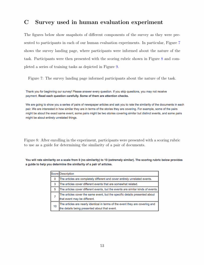
C Survey used in human evaluation experiment

The figures below show snapshots of different components of the survey as they were pre-

sented to participants in each of our human evaluation experiments. In particular, Figure 7

shows the survey landing page, where participants were informed about the nature of the

task. Participants were then presented with the scoring rubric shown in Figure 8 and com-

pleted a series of training tasks as depicted in Figure 9.

Figure 7: The survey landing page informed participants about the nature of the task.

Figure 8: After enrolling in the experiment, participants were presented with a scoring rubricto use as a guide for determining the similarity of a pair of documents.

53

Figure 9: In the first training task of the survey, participants were ask to read and scorea pair of articles and were then informed that the anticipated score for this pair was zero.Specifically, they were told “We think these articles’ similarity is 0 out of 10. The first articleis related to macaroni and cheese, while the second article is about a murder trial.”

54

D Sensitivity of match quality scores to the population

of respondents

To determine the generalizability of the match quality ratings obtained from our survey

experiment, we compare two identical pilot surveys using respondents from two distinct

populations. The first pilot survey was administered through Mechanical Turk, and the

second pilot was administered through the Digital Laboratory for the Social Sciences (Enos

et al., 2016). For each survey, respondents were asked to read and evaluate ten paired articles,

including one attention check and one anchoring question. Each respondent was randomly

assigned to evaluate eight matched pairs from a sample of 200, where this pilot sample was

generated using the same weighted sampling scheme described above. Figure 10 shows the

average match quality scores for each of the 200 matched pairs evaluated based on sample

of 337 respondents from Mechanical Turk and 226 respondents from DLABSS. The large

correlation between average matched quality scores across samples (ρ=0.88) suggests that

our survey is a useful instrument for generating consistent average ratings of match quality

across diverse populations of respondents. In particular, even though individual conceptions

of match quality may differ across respondents, the average of these conceptions both appears

to meaningfully separate the pairs of documents and to be stable across at least two different

populations.

55

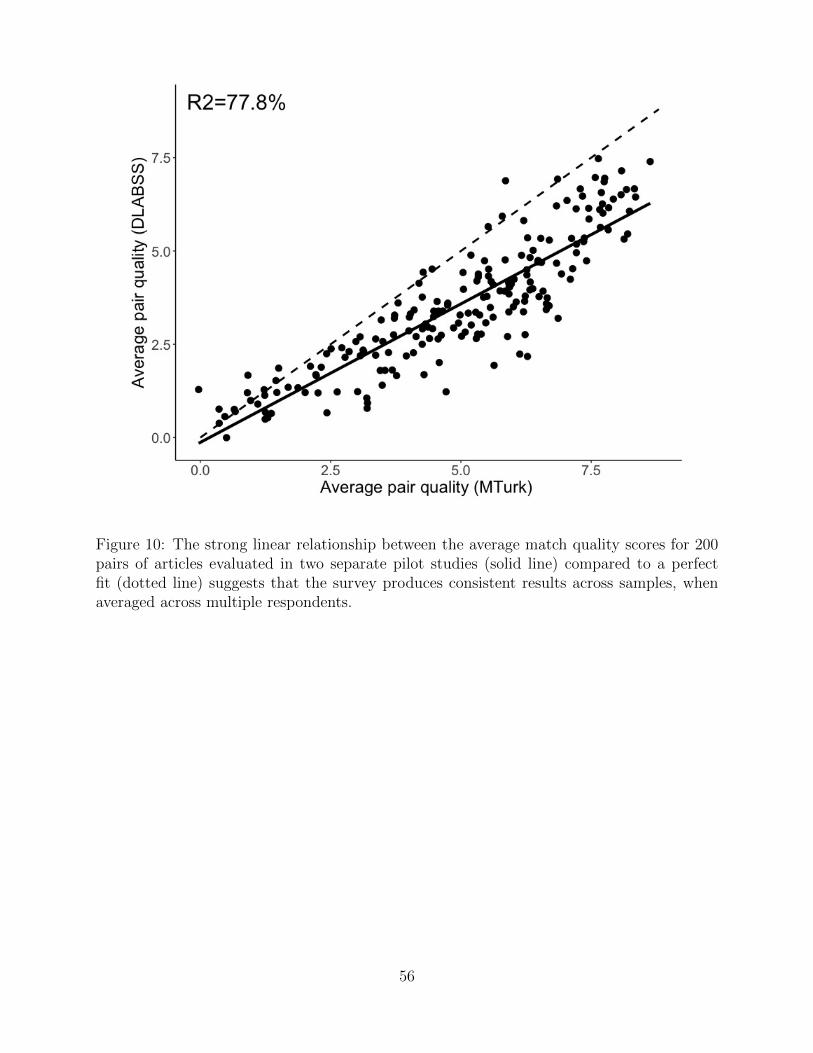
Figure 10: The strong linear relationship between the average match quality scores for 200pairs of articles evaluated in two separate pilot studies (solid line) compared to a perfectfit (dotted line) suggests that the survey produces consistent results across samples, whenaveraged across multiple respondents.

56

E Technical details of the evaluation of match quality

of pairs of news articles

In this section we more fully describe the design and analysis of the human evaluation

experiment for the newspaper matching example. We start by discussing how we generated

our sampling strategy and weights, and then discuss how we used model-assisted survey

sampling to estimate average match quality for the different methods along with associated

uncertainty.

E.1 Details of the sampling design

The study presented in this paper is in fact a replication study as our initial study did

not directly assess all procedures considered (in particular, we did not initially evaluate the

Word2Vec procedures). We therefore designed our second study to both directly extend our

findings, verify the prior results, and further investigate the predictive accuracy of our models

to out-of-sample pairs. In order to achieve this, we designed a sampling scheme that has

three components: (1) we sampled 4 pairs from each procedure considered, (2) we directly

sampled pairs that were previously evaluated to assess the stability of the evaluation process,

and (3) we sampled pairs not selected by any method to examine differences between selected

and non-selected pairs. The first stage sampled pairs with weights based on the predicted

quality of the pairs in order to sample predicted high-quality pairs more heavily. We used

the prior study’s fit predictive model to generate these predictions. The second and third

stage sampled a fixed number of pairs within each tier of quality (from 0 to 8+) to see the

full range of pair qualities in our sample (simple random sampling would not work since

the vast majority of pairs are scored as quality 1 or lower). This overall process resulted in

a sample of 505 pairs that fully represents all possible pairs (selected and not). For each

pair we have an initial predicted quality score, a sampling probability πi, and an associated

sampling weight wi ∝ 1/πi.

57

Because many of the procedures generally select the same high-quality pairs, the sequen-

tial sampling of 4 pairs for each procedure tends to give many of the same pairs back. This

is by design, and means that our sample primarily consists of pairs shared by multiple pro-

cedures which gives greater precision in estimating these procedures’ average quality. We

simply take the unique set of pairs sampled as our final evaluation sample.

We calculate the actual sampling weights of each pair for this scheme using simulation.

In particular, we conduct our sampling scheme 100,000 times and calculate how often each

pair is selected into the sample. These provide (up to monte carlo error) the true selection

probabilities πi; inverting them provides the true sampling weights wi. For the out-of-

matched pairs sampling stage (3), we averaged these final weights across groups of pairs that

all have the same probability of selection to increase precision.

The stage (1) sampling scheme intentionally induces selection bias into the sample by

discouraging rare pairs, especially singleton pairs, which are expected to be low quality

with little variability, in favor of pairs that are identified by multiple matching procedures.

Regardless, because the sampling probabilities are fixed a-priori, weighted averages of the

pairs’ match quality gives good estimates of the average quality of the pairs selected by each

procedures; this approach is simply classic survey sampling as described in, e.g.,Sarndal et al.

(2003). All this complexity in the sampling design is to ensure that the sample evaluated

is targeted to give information on as many procedures as possible, a difficult task when

evaluating 130 procedures with a sample size of about 500.

E.2 Estimating pair and procedure quality.

Let ut,c denote a potential pairing of treatment and control documents, where t is the index of

the treated unit and c is the index of the control unit. In our evaluation study, t = 1, . . . , 1565

and c = 1, . . . , 1796. For matching procedure j, let Rj denote the set of nj matched pairs

of articles identified using procedure j. The set of all unique pairs selected by any of the J

procedures considered in the evaluation experiment, denoted R, is defined by the union of

58

these subsets:

R = ∪Jj=1Rj.

We index the pairs with i = 1, . . . , N .

The frequency of how often each pair ui in R was selected by a procedure is:

Fi =J∑

j=1

1{ui ∈ Rj},

where 1{i ∈ Rj} is an indicator variable taking value 1 if pair ui is identified using matching

procedure j and 0 otherwise.

From the human evaluation, we, for each element i of S, where S is the set of all sampled

pairs, observe mi similarity ratings, qobsi,1 , . . . , qobsi,mi

where qobsi,· ∈ [0, 10]. We estimate the match

quality for each evaluated pair i using the average of observed ratings for that pair, qobsi .18

We wish to estimate, for each procedure, the finite-population quantities of the average

true quality of the pairs selected. In particular, if we let qi be the average quality score score

we would see if we had an arbitrarily large number of human respondents evaluate that pair,

our targets of inference are, for each procedure j,

Qj =1

Nj

∑ui∈Rj

qi.

The Qj are population quantities of how the matching procedure did in the specific context

considered. This estimand does not necessarily take into account how the methods would

perform on other corpora, even ones similar to this one.

To estimate Qj for any matching procedure j in our evaluation we use a weighted average

of the match quality estimates across the pairs contained in Rj ∩ S, where weights for each

18We also explored modeling these ratings to account for rater effects and variable number of ratings perquestion, but as the results were essentially unchanged, elected to use the simple averages.

59

pair are equal to the inverse probability of being sampled:

Qsamp,j =1

Zj

∑ui∈Rj

1

πiSiq

obsi with Zj =

∑ui∈Rj

1

πiSi. (1)

with Si an indicator of whether pair i was sampled for evaluation, with sampling probability

πi, and Zj a normalizing constant. This is a simple Hajek estimator and is known to have

good properties.

Unfortunately, despite the sampling scheme, some of our methods only had a small

number of pairs sampled for evaluation. Estimating the average match quality for such

procedures could therefore be fairly imprecise. We address this by using our model for

predicting the match quality of a pair of documents based on different machine measures

of similarity to construct model-assisted survey sampling estimators that use the predicted

qualities to adjust these estimated average quality scores. We describe this analysis approach

next.

E.3 Improving the estimates of procedure quality.

To enhance our predictions of match quality for our procedures, we use a model trained on

the pairs in Spre, the sample collected in our initial study, to calculate the predicted match

quality, qi for all pairs i = 1, . . . , N . These qi are fixed, and do not depend on the analyzed

(i.e., second) random sample. We can use these predictions to adjust our estimates of the

average quality of all pairs for each procedure using survey sampling methods.

In particular, our model adjusted quality for procedure j is

Qadj,j =1

nj

∑ui∈Rj

qi +1

Zj

∑ui∈Rj

Si

1

πi

(qobsi − qi

)

Here qi is the predicted quality based on the initial sample. Note the first term in the above

is a fixed constant, not dependent on the sample. The second term is random, depending on

60

the sample, and, ignoring the small bias induced by Zj being random, we see the expected

value is

E[Qadj,j

]≈ 1

nj

∑ui∈Rj

qi +1

E[Zj

] ∑ui∈Rj

E[Si

1

πi

(qobsi − qi

)]

=1

nj

∑ui∈Rj

qi +1

E[Zj

] ∑ui∈Rj

E [Si]1

πi

(E[qobsi

]− qi

)=

1

nj

∑ui∈Rj

qi = Qj.

This is a model-adjusted estimate; the first summation gives the predicted average quality

of the method. The second summation adds an adjustment based on the residuals for the

actually sampled and evaluated pairs; this adjustment makes the overall estimate effectively

unbiased19 regardless of whether the predictive model is useful, predictive, or even correct.

The more the predictive model aligns with the actual measured values, however, the more

precise our estimates will be (as the residuals and adjustment part will get smaller and

smaller as predictive accuracy grows).

E.4 Uncertainty estimation

Classic survey sampling results allowed us to estimate each procedure’s average quality with

the estimated qualities of our sampled pairs. We can also increase the precision of these

estimates using model adjustment, using the predicted quality scores to adjust the same by

population averaged characteristics. In both cases, the next step is to obtain appropriate

uncertainty estimates (standard errors) for these point estimates. Unfortunately, the task

of appropriately calculating uncertainty in this context for both the raw estimates and the

model-adjusted estimates is a surprisingly difficult and subtle problem. In particular, while

there are classic survey sampling formula that can be used to calculate uncertainty, they

19The bias is purely from using a Hajek rather than Horvitz-Thompson estimator, and comes from thenormalizing Zj being a random quantity. It is not a function of model misfit or misspecification.

61

are asymptotic and are sensitive to extreme weights (which we have). This creates some

perverse results (i.e. near zero standard errors) for some of the procedures that only had

a few pairs sampled. To avoid this we, by instituting a homoscedastic assumption for the

error terms, did a parametric simulation to calculate uncertainty in order to work around

this problem. This procedure captures the variability induced by the varying sample weights

and the measurement error due to the human evaluation. We describe this next.

Uncertainty estimates for the raw quality estimates. For the unadjusted quality

measures, we estimate uncertainty using the principles of a case-wise bootstrap with some

modifications. In particular, especially for those methods with very few (e.g. 4) sampled

pairs, estimating the variability of quality of the pairs via case-wise bootstrap is unreliable

unless we pool or partially pool estimates of variability across the different methods.

To see this consider a hypothetical method with 4 of its pairs sampled, 1 with very high

weight due to being a rare pair and 3 with a low weight due to being selected by most

methods. Any bootstrap sample that includes the high weight unit will essentially give an

average quality score close to that of the high weight unit. Even bootstrap samples with

multiple draws of the high weight unit will still get nearly that same average quality score

since the values of these large elements will all be the same. Across bootstrap samples, this

will give low variability, i.e., seemingly high precision. It does not take into account the

variability of scores we might have actually seen across other units of similar weight. We

address this with the a parametric approach that we describe next.

We first assess the typical variability of the quality scores of pairs within the procedures.

For the unadjusted quality scores of the individual pairs we first calculated an estimate of

the standard deviation of scores within a given match method (we did this by calculating

the weighted standard deviation of scores). We then took the median of these values as our

measure of within-method variation of pair quality. We use the median to avoid the impact

of the extreme standard deviations due to the methods with small samples of pairs.20

20We actually calculated this (pooled) standard deviation a variety of ways and took the largest to be

62

To calculate standard errors for our methods, we then simulated the pair sampling step

followed by the scoring of sampled pairs step by first selecting pairs using the original sam-

pling strategy, and then generating pseudo-quality scores with the same variance as we

generally saw for pairs selected by a method. We then calculated the overall pseudo-quality

for each of our methods based on these scores and associated sample weights. Our standard

errors are then the standard deviation of these generated overall pseduo-quality scores.

To compare, we also conducted a simple case-wise bootstrap. Here we sampled the evalu-

ated pairs with replacement and calculated each methods’ quality score using the bootstrap

sample, finally obtaining standard errors using the standard deviation of the resulting val-

ues. This approach works well for those methods with 10 or more sampled pairs. Overall,

our parametric approach generally produced larger standard errors, which is a mixture of

the overall conservatism of our approach and of the aforementioned issue of the naıve ap-

proach giving small standard errors those methods with few pairs and a few high-weight pairs

that dominate the overall quality measure. We thus report our parametric simulation-based

standard errors.

Uncertainty for the model-adjusted approach. For the model-adjusted case, we again

worried about those methods with few samples having less variability due to small numbers

of high weight units giving nearly the same model adjustment with each step. We therefore

follow the above process, but instead of generating synthetic outcomes we generated synthetic

residuals by generating normally distributed noise with variance equal to the variance of the

original residuals from our predictive model. These simulated residual-based standard errors

were again conservative when compared to the naıve case-wise approach for those procedures

with enough selected pairs to make this comparison.

Remarks. All our uncertainty estimation methods capture the uncertainty in the pair

quality evaluation process as the variability of the pairs’ quality scores captures both the

maximally conservative.

63

measurement error and the structural variation of the pairs themselves. In our plots, we

report the simulation-based standard errors for the model adjusted estimates. As noted in

the text, the model-adjusted quality scores themselves were generally similar to unadjusted

(for the directly evaluated methods where we had both scores), and the differences between

the two had no impact on our overall findings.

For methods that we did not initially identify for our human evaluation, we could calculate

a predicted quality based on our model of

Qpred,j =1

nj

∑ui∈Rj

qi.

This is extrapolation, however. If the new procedure was selecting pairs that systematically

were better than predicted, for example, this extrapolation would be biased. Even if such

a new method happened to use some pairs randomly selected for evaluation, we cannot use

the survey adjusted Qadj,j or raw estimate Qsamp,j since the pairs not in the sampling frame

had no chance of selection. One could create a hybrid estimator by splitting the sample into

potentially sampled, but we do not explore that further here.

E.5 Prior evaluation study details

As mentioned above, we performed an initial full study on an initial subset of the matching

procedures considered (in particular, we did not initially evaluate the Word2Vec procedures).

Overall, this study produced the same results as our final study.

We sampled pairs differently for our initial study. In particular, we did not have baseline

predicted quality scores to calculate sampling weights from. We therefore, to produce a

representative sample of matched articles for evaluation, did not take a sample from each

procedure’s pair list but instead took a weighted random sample of 500 pairs from the union

of these lists, R, with sampling weights roughly proportional to Fi, where Fi is the number

of times pair i was selected by a procedure. Because singleton pairs comprised over 75% of

64

the pairs in R, we further downweighted pairs with Fi = 1 by a factor of 5. Our overall

sampling probabilities for pair i were then

wi ∝

0.20 if Fi = 1,

Fi otherwise.

We then calculated true sampling probabilities and weights via simulation as described above

(due to high weights for some pairs and the sampling without replacement these initially

weights are not truly proportional to inverse probability of selection).

65

F Notes on the sample and unadjusted human exper-

iment results

The final evaluation sample consisted of 33 pairs that were originally evaluated in the initial

evaluation, 50 pairs that were not identified by any matching method considered, and 422

pairs that were used by at least one matching method evaluated. The sampling weights

for those pairs that were selected by at least one method ranged from 0.02 to 10.7, with a

median of 0.23. This corresponded to selection probabilities ranging from 1 in 1000 to 77%.

25% of the pairs had less than a 1% chance of being selected. The very rare pairs tend to

come from the propensity score methods that had a large number of low-quality matches.

Across procedures, some had only 4 pairs sampled, and some had up to 100. The average

was 28 pairs.

The standard deviation of quality scores did depend on the sampling weight, with a

standard deviation of around 2.5 for low pii and 1 for the highest pii. On the other hand,

the standard deviation of scores for very low and very high predicted qualities was less than

0.5, rising to around 1.6 for pairs predicted to have a quality of 5. Within a given procedure,

scores tended to have a standard deviation of around 2.37, for those procedures with 10 or

more pairs sampled. If we look across all procedures the median decreases markedly due to

poor estimates for small sample sizes. We used 2.37 in our simulation.

For the residual scores, residuals had a lower standard deviation near the endpoints (due

to truncation) and peaked at around 1.6 for the middle scores. We therefore use a residual

standard deviation of 1.6 in our simulations to calculate our standard errors, which will be

generally conservative. Even with this conservative approximation, we are explaining 55%

of our variation with our predictive score.

Figure 11 shows the simple weighted average match quality of the directly evaluated

pairs sampled for each of the 130 procedures considered in the evaluation experiment. The

nominal 95% confidence intervals are from standard errors calculated from the parametric

66

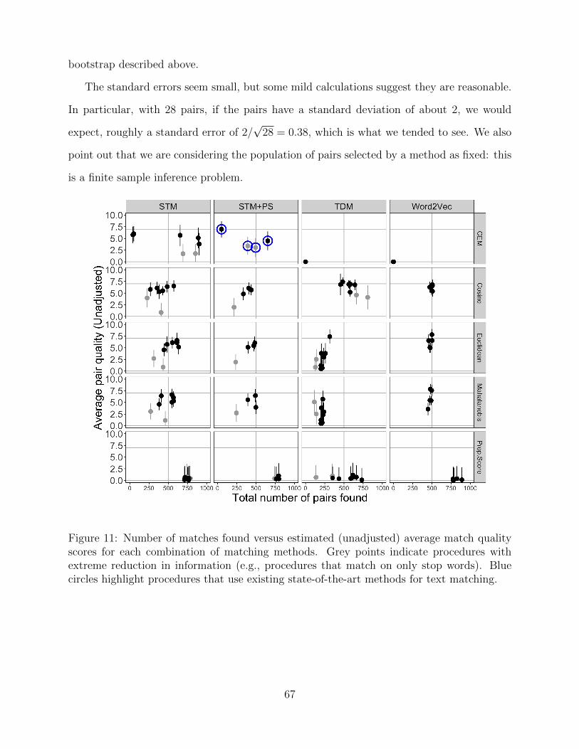
bootstrap described above.

The standard errors seem small, but some mild calculations suggest they are reasonable.

In particular, with 28 pairs, if the pairs have a standard deviation of about 2, we would

expect, roughly a standard error of 2/√

28 = 0.38, which is what we tended to see. We also

point out that we are considering the population of pairs selected by a method as fixed: this

is a finite sample inference problem.

Figure 11: Number of matches found versus estimated (unadjusted) average match qualityscores for each combination of matching methods. Grey points indicate procedures withextreme reduction in information (e.g., procedures that match on only stop words). Bluecircles highlight procedures that use existing state-of-the-art methods for text matching.

67

G Template Matching and Sensitivity Analyses for Me-

dia Bias Application

To evaluate the robustness of our findings, we performed a series of sensitivity checks to

assess how our results and subsequent conclusions change when using different specifications

of the matching procedure. Figure 12 shows the results produced by three alternative text

matching methods. These robustness checks highlight the importance of the specification of

the matching procedure: weaker methods (i.e., methods that produce low quality matches)

typically lead to weaker inferences. For example, the results produced from template match-

ing using the Mahalanobis distance metric on a vector of 100 topic proportions show generally

smaller changes in average favorability within each source before and after matching than the

results shown in Figure 4. The null results in this case provide further evidence in support of

the claim that text matching is an effective strategy for reducing differences in the observed

biases across news sources that are due to topic selection.

As a final robustness check of the results based on our template-matched sample, we

performed the following consistency test. First, we randomly generated 10,000 pairs of

documents containing 150 randomly selected articles from each news source. In each iteration

of random sampling and for each news source, we then calculated the average favorability

scores towards Democrats and Republicans within the matched sample. Figure 13 shows

the distributions of these favorability scores for each news source after 100 iterations of

random matching. Finally, we calculated the total change in favorability observed after

matching in each iteration, averaged across all 13 sources. More formally, for each iteration

i = 1, . . . , 10000 we calculated the test statistic:

Ti =1

13

13∑j=1

(|Y dem

j − Y demj,Mi|+ |Y rep

j − Y repj,Mi|),

where Y demj and Y rep

j denote the average favorability scores toward democrats and repub-

68

licans, respectively, for all articles corresponding to source j in the original, unmatched

sample. Quantities Y demj,Mi

and Y repj,Mi

denote the partisan favorability scores averaged across

the set of 150 articles from source j that were selected by random matching in iteration

i. The sampling distribution of this test statistic provides a reference for values of the test

statistic that may occur when comparing randomly selected sets of 150 articles across these

13 sources. Therefore, by comparing the value of our observed test statistic based on the

results of our template-matching procedure described in Section 5 to the randomization dis-

tribution defined by T , we can estimate the probability that our template-matched results

are due to random chance. Our results from this randomization test indicated that tem-

plate matching on text removes a significant amount of the bias observed across sources that

remains after adjusting for differences in topic selection (p=0.004).

69

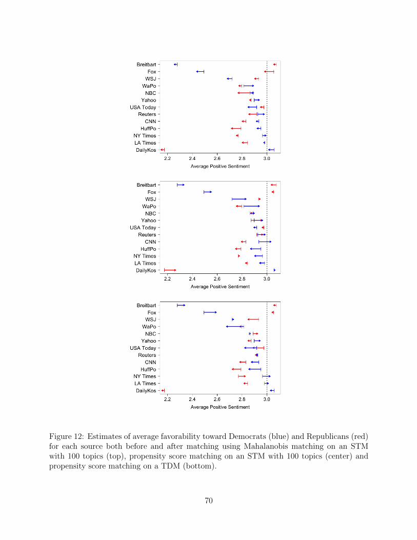
Figure 12: Estimates of average favorability toward Democrats (blue) and Republicans (red)for each source both before and after matching using Mahalanobis matching on an STMwith 100 topics (top), propensity score matching on an STM with 100 topics (center) andpropensity score matching on a TDM (bottom).

70

Figure 13: Estimates of average favorability toward Democrats (blue) and Republicans (red)for each source for 100 iterations of random matching. Blue and red lines represent theaverage favorability scores before matching for Democrats and Republicans, respectively.

71