master’s thesis the price of cryptocurrencies: an

Master’s Thesis

The Price of Cryptocurrencies: AnEmpirical Analysis

Chair of Economic TheoryUniversität Bern

Supervised by:Professor Dr. Aleksander Berentsen

Author:Joel WiedmerSubmission Date: July 06, 2018

Abstract

In this paper, we analyze cryptocurrency price determinants suggestedby literature using a panel of 17 cross-sections. We employ unit root andcointegration tests, and estimate the effects with Vector Error Correc-tion Models, Dynamic OLS and Fully Modified OLS. Causality flows areexamined by weak exogeneity and Granger causality tests. We confirmMetcalfe’s Law, which identifies the value of a network to be propor-tional to the number of its nodes. We show that community factors andsearch engine queries have a cointegrating relationship with market cap-italization. Our findings further suggest that the influence of innovationpotential is heterogeneous across cross-sections. Moreover, we observethat the direction of causality often flows from market capitalization tothe variable which is believed to be the determinant, but not vice versa.

1

Contents

1 Introduction 1

2 Review of literature 3

3 Empirical Evidence 8

3.1 Data . . . . . . . . . . . . . . . . . . . . . . . . . . . . . 8

3.2 Econometric Methodology . . . . . . . . . . . . . . . . . 14

3.3 Results . . . . . . . . . . . . . . . . . . . . . . . . . . . . 26

4 Discussion 35

References i

Appendix v

PlagiatserklärungBern, July 6, 2018

Ich bezeuge mit meiner Unterschrift, dass meine Angaben über die beider Abfassung meiner Arbeit benützten Hilfsmittel sowie über die mirzuteil gewordene Hilfe in jeder Hinsicht der Wahrheit entsprechen undvollständig sind. Ich habe das Merkblatt zu Plagiat und Betrug gelesenund bin mir der Konsequenzen eines solchen Handelns bewusst.

I would like to thank Bobby Ong and Teik Ming Lee from CoinGecko forkindly providing the necessary data to make this thesis happen. More-over, I would like to thank Prof. Dr. Aleksander Berentsen and Dr.Fabian Schär for their valuable inputs and feedback.

I

1 Introduction

Since its introduction by Nakamoto (2008), Bitcoin has increasingly gain-ed interest. The price rally in late 2013 attracted mainstream attention,not only towards Bitcoin specifically but also the underlying technology,Blockchain, due to its potential disruptive impact. Blockchain technologyprovides a cryptocraphically secure way of sending digital assets, withoutthe need for trusted third parties like banks. Different features and inno-vations related to Blockchain are arising with a fast pace, such as smartcontracts which promise to automate processes distributing contents ofa will within the banking industry, compliance and claims processing,and possibly innovations in many other fields. A survey by the Inter-national Securities Association for Institutional Trade Communication,ISITC (2016), reveals that 55% of firms are monitoring, researching or al-ready developing solutions for Blockchain technology. Amongst servicesonly in the banking sector to be potentially disrupted by Blockchain arepayments, clearance and settlement systems, securities, loans and creditas well as fundraising. The latter is called initial coin offering (ICO) andprovide Blockchain companies with immediate access to liquidity, com-pletely independent from traditional third party services. Consequently,a lot of cryptocurrencies and -assets1 have emerged, providing innovativefeatures related to the topics mentioned above. Most of the innovationsare somehow related to improving speed, robustness and privacy. At thisstage, it has to be mentioned that Bitcoin played a predominant role inthe market and still is the largest issuer, if measured by market capital-ization. However, its dominance decreased gradually over the past years.In the beginning of January 2014, Bitcoin had a market share (definedas market capitalization in percentage of total market capitalization) of90%, which receded to current 36% according to CoinMarketCap (2018c).The second largest is the Ethereum network with 17%, followed by Rip-1Hereinafter, we rely on the following definition according to Merriam-Webster (2018):Cryptocurrency is any form of currency that only exists digitally, that usually hasno central issuing or regulating authority but instead uses a decentralized systemto record transactions and manage the issuance of new units, and that relies oncryptography to prevent counterfeiting and fraudulent transactions. We use theterm cryptoasset as a synonym in this thesis.

1

ple (7%) and Bitcoin Cash (6%). The market shares of the remainingcurrencies within the top ten move between 1% and 2%. In total, the 10largest crypto-assets amount to 75% of total market capitalization, whichleaves a considerable part to all other Altcoins2. Despite their rising rel-evance, research in the past years has focussed on Bitcoin. At the sametime, existing studies for cryptocurrencies include three to five currenciesand/or rather short time spans in their analysis. Thus, the motivation ofthis thesis is to shed light on the determinants of cryptocurrency pricesfrom a empirical perspective, with a focus on the direction of causalityflows. By construction, the supply side of the cryptocurrency market isfixed and consists of a predefined range of tokens or units which is an-nounced in the act of an ICO. Thus, we are particularly interested in thequestion of what the determinants for demand are. In order to this, welook at research done so far in the field of cryptocurrencies and evaluateits results. Next, these insights are used and time series data is gatheredin order to measure the relationship of these proxies and the price of acryptocurrency. Due to the fact that cryptocurrencies have a predefinedsupply (which is often mined during a certain time period harwired in thesource code) varying from one another, using price as dependent variablewould lead to biased results. Consequently, this variable is standardized.The explanatory variables are derived from literature discussed in thesubsequent chapters and are selected upon criteria related to Metcalfe’sLaw, development activity, community factors and search engine queries.The data is then grouped to a time series panel consisting of 17’299 dailyobservations. Next, we follow the standard procedure in the literaturefor non-stationary time series (which is a predominant property in ourdata) and test the series for cointegration. In order to measure the po-tential long-run relationship and short-term dynamics, we use a VectorError Correction Model (VECM) as well as Fully Modified Least Squares(FMOLS) and Dynamic Least Squares (DOLS) to test the robustness ofthe estimates. It is tested for weak exogenity and Granger causality tofurther establish causalities amongst the variables. Finally, we discuss2The term Altcoin is an abbreviation for alternative coin, which means any cryp-tocurrency other than Bitcoin

2

the outcome of the estimations. The remainder of the thesis is organisedas follows: In Chapter 2, we review literature related to the topic and jus-tify the research topic. In chapter 3, we discuss in detail the data selectedfor the analysis and the econometric approach and present the estimationresults. Lastly, the results are discussed in chapter 4. Together with thisthesis, we provide a broad database of estimation results for the differentcryptocurrencies besides panel estimation results.

2 Review of literature

Before it is looked at literature linked specifically to cryptoassets, a briefdigression may be allowed. As put out by White (2015), the cryp-tocurrency market is comparable to a market of competing private ir-redeemable monies in the sense of Hayek (1976). This market is char-acterized by financial institutions which create currencies that competefor acceptance, where stability in value is presumed to be the decisivefactor for acceptance. Users will choose the currency they expect is themost competitive. However, there is big caveat: Hayek imagined thatthe issuer of a successful irredeemable currency would retain discretionto vary its quantity. The issuer would promise a stable purchasing powerper unit, but this promise would appear to be time-inconsistent as theone-time profit of issuing new money would exceed the return of stayingin business and as a result, the public would not believe the promiseto begin with, hence giving money zero value in equilibrium. For a de-tailed discussion, see e.g. Taub (1985) or White (1989). In order to solvethis problem, the privately issued money comes along with a money-back guarantee (a price commitment) such as gold given by the issueras proposed in White (1989). The alternative solution to this problemidentified by Coase (1972) is a quantity commitment, i.e. the issuer bindsitself to produce only a limited amount of money. However, to make acredible promise not to exceed the self-imposed quantity limit is difficultif not impossible to put in place, resulting in the public not believingin the commitment. But the features of the crypto-market are different

3

from what Hayek and other economists back in these days have imagined,i.e. the possibilities have changed with the introduction of Blockchaintechnology. As the issuer of a cryptoasset programs the quantity com-mitment into the source code, he provides a credible contractual promisenot to exceed the limit defined in the first place. The source code is pub-licly available and the quantity limit defined therein is verified through apublic ledger. Due to the availability of the source code, the Blockchaintechnology is basically accessible to everyone and therefore, the barriersto enter the crypto-market are low. Consequently, there was an tremen-dous increase of cryptoasset issuers in the past years: CoinMarketCap(2018b), an online price tracker for cryptocurrencies, currently lists 1600issuers. As outlined in the first chapter, the competition has intensifiedwithin the past few years. Bitcoin has lost its predominant role, with amarket share of roughly one third by today compared to 90% in the earlyyears of Bitcoin. The subsequent questions is, obviously, by which factorsusers determine to buy these coins. For the sake of its dominance, a lot ofresearch up to this date focused solely on Bitcoin. Nevertheless, there isa number of publications related to Altcoins and the cryptoasset marketas a whole. White (1989) states in his analysis of the cryptocurrencymarket that Bitcoin was the first of its kind (decentralized peer-to-peerexchange, quantity commitment embedded in an open source code, andshared public ledger), but soon there were Altcoins coming alive withimproved features, mostly in terms of speed, robustness and privacy. Asthere was demand for these new cryptocurrencies as well as subsequentrise in market capitalization, their value seemed justified. However, therewere several coins which had an immense price rally after launch, eventu-ally declining not long after that. This reminds of the dotcom collapse inthe beginning of 2000, where the extreme growth in the usage and adap-tion of the internet caused excessive speculation and bubbles. Lansky(2016) analyses the price development of cryptocurrencies on a broadbasis and puts together a database consisting of over 1200 currencies.Next, he was looking for the largest increases and drops as well as theirrespective causes. As reasons for the price drops, he names the burst of abubble in late 2013 (without going into detail), the early sale of founders

4

short after an ICO causing a demise and lastly the fact that some cur-rencies introduced technical innovations, but were overcome quickly byother currencies in this regards. The author identifies the reasons forthe largest price increases within the fact that a cryptocurrency eitherbrought a significant technology innovation or if the cryptocurrency of-fered a decentralized service demanded by users, a team of people (whichhe calls foundation) managed the development and promotion amongstthe community. These findings are interesting inasmuch as they are inline with the aforementioned characteristics of a market of competingcurrencies in the sense of Hayek, where technological innovation and thecommunity base seem to be decisive factors for users. Farell (2015) isanalysing the cryptocurrency industry and comes to the conclusion thatmajor factors which affect growth are government regulations as wellas public perception and retailers accepting coins. Similar to Lansky(2016), there is no quantitative support for the arguments. Ong et al.(2015) are evaluating the potential of alternative cryptocurrencies by aquantitative analysis of community support, developer activity and liq-uidity. However, there was very few data (less than two months of dailyobservations) available, thus making proper inference difficult if not im-possible. S. Wang and Vergne (2017) show that innovation potential ispositively associated with weekly returns for a panel of 5 cryptocurren-cies and the time span of one year. They also find that public interest(measured as standardized metric consisting of bing search results andAlexa web traffic ranking) is negatively associated with weekly returnsand negative publicity has no significant relationship. For the latter, theauthors counted how many media articles were published with the cryp-tocurrency and a negatively associated keyword. Another strand in theliterature for cryptocurrencies is to consider the Blockchain as a networkwhich can be valued according to Metcalfe’s Law. Four decades ago, Met-calfe (2013) suggested at the example of the ethernet that the value of atelecommunications network is proportional to the nodes of the networksquared. This example has lately been tested for social networks such asFacebook as well as cryptocurrencies. Alabi (2017) shows that Bitcoin,Ethereum and Dash follow Metcalfe’s Law. He states that this could be a

5

potential identification scheme for bubbles, as it is shown that those pricesurges which are not accompanied by any commensurate increase in thenumber of participating users return to the path which is characterizedby Metcalfe’s Law. Finally, we also look at research which was done so farwith regard to only the Bitcoin network. Ciaian, Rajcaniova, and Kancs(2016) summarize the three main determinants of the Bitcoin price iden-tified in the literature up to now as follows: Market forces of supply anddemand, attractiveness indicators and global macroeconomic and finan-cial development. Most of the papers include a range of variables for thefirst determinant, supply and demand factors within the Bitcoin ecosys-tem, in their models. Kristoufek (2015) incorporates a broad range ofsuch factors into a wavelet coherence analysis and finds that trade volumeand trade transactions have significant relationships with changing signsover time, as well as that price is positively correlated in the long run withboth hash rate and difficulty. Ciaian, Rajcaniova, and Kancs (2016) con-firm the impact of such factors and find that demand side variables (suchas number of transactions, number of addresses) appear to excert a morepronounced impact on Bitcoin price than the supply side drivers (e.g.number of Bitcoins). Bouoiyour and Selmi (2015) show by employing anARDL bounds testing approach that the exchange-trade ratio and theestimated output volume affect positively and significantly the Bitcoinprice, while monetary velocity and the hash rate have no impact. In thelong-run, output volume bcomes statistically insignificant and the effectof exchange-trade ratio becomes less strong. On the other hand, hashrate becomes significant. When it comes to attractiveness indicators, itwas foremost search engine queries that was used as a proxy. Kristoufek(2013) believes that the demand side of the market is not driven by anexpected macroeconomic development of the underlying economy - asthere is none - and its price is simply determined by expected profits ofholding the currency and selling it later. The author therefore concludesthat the currency price is solely driven by the investors’ faith in the per-petual growth. To measure this faith, he uses Google and Wikipediaqueries as a proxy for investors’ sentiment. Ciaian, Rajcaniova, andKancs (2016) confirm these findings and additionally show that "new

6

members" and "new posts" on online Bitcoin forums have a significantimpact on Bitcoin price. Lastly, macroeconomic variables where testedto have an impact on the Bitcoin price. Some papers, such as Bouoiyourand Selmi (2015) and Ciaian, Rajcaniova, and Kancs (2016) come to theconclusion that the inclusion of macroeconomic variables like oil price,Dow Jones index and exchange rates have no impact on the Bitcoin price.By contrast, J. Wang, Xue, and Liu (2016) show that the oil price andstock price index do have an influence. Smith (2016) claims Bitcoin to bedigital gold and shows that nominal exchange rates implied by the Bit-coin price are highly cointegrated with the conventional exchange ratesand that there is a unidirectional causality which flows from conventionalexchange rates to Bitcoin implied rates, concluding that floating nominalexchange rates are a major source of price volatility in the Bitcoin mar-ket. As one can see, some results contradict each other and there doesnot seem to be a clear consensus yet upon what the determinants of theBitcoin price are. Vockathaler (2015) discusses this issue and comes tothe conclusion that some results are drastically different when they arere-tested after the results have been published. Moreover, he finds thatunexpected shocks are the largest contributor to the price fluctuations ofBitcoin. In this thesis, we aim at testing factors which might influencethe price of a cryptocurrency, not only the Bitcoin price. We thus relyon conclusions drawn from the analysis of the cryptocurrency marketand combine these different strands of literature. First of all, results forproxies related to Metcalfe’s Law seem to be quite robust across studies.Alabi (2017) shows a clear correlation between addresses squared andvalue for three currencies, but also daily trading volume and number ofaddresses in Bitcoin-only research shows evidence for this relationship.Secondly, White (2015) introduces the theoretical framework of a mar-ket where currencies compete amongst each other by introducing new,innovative features to convince users to choose their units above others.Lansky (2016) argues that the reason for failure of a cryptocurrency is tobe overtaken by other currencies with superior innovations, while at thesame time price surges are often due to significant technology innovation.In line with J. Wang, Xue, and Liu (2016), we include proxies for inno-

7

vation potential in our analysis. Another factor which was confirmed tohave an influence is the community behind a cryptocurrency, as put outby e.g. Lansky (2016). Moreover, we can motivate the inclusion of thisfactor by Metcalfe’s Law: The larger and stronger its community, thehigher should be a currency’s adoption. Lastly, we include search enginequeries in order to test if their relationship with a cryptocurrency pricehas the same character as in research done so far.

3 Empirical Evidence

3.1 Data

In the following chapter, the variables used for analysis are described indetail as well as how and where they were retrieved. Overall, we usedmarket capitalization as dependent variable and 10 explanatory variablesaccording to the factors outlined in the previous chapter.

Dependent variable: Market capitalization

A lot of studies mentioned in the literature review section use price asdependent variable. However, this would be misleading in our case as weaim at comparing different cryptocurrencies. Due to the fact that everycurrency has a pre-defined (maximum) supply of coins which is quitedifferent from one another, we have to find a standardized figure whichmakes the currencies comparable. In order to do this, we use marketcapitalization (marketcap) as proxy for the value of a cryptocurrency.For the sake of data availability as well as the logic behind it, we rely onthe definition provided by CoinMarketCap (2018a) which tracks marketcapitalization as product of circulating supply and price. Therein, price iscalculated by taking the volume weighted average of all prices reported ateach market. Circulating supply is defined as the number of coins that arecirculating in the market and in the general public’s hands. Therefore,coins that are locked, reserved, or not able to be sold on the public

8

market can’t affect the price and are thus not included in the calculationof market cap. The time series are retrieved from the aforementionedsource. Within the context of cryptocurrencies, a recurrent behaviour ofmarket participants is the formation of so called pump and dump groups.Holders of a (often, but not only a rather less-popular) token artificiallyinflate the price of this currency in hope that other investors will pick itup too as a result of their "fear of missing out". By the time the coin hasreached a certain targed range, the initial buyers begin to sell and earn aquick profit. However, as there is no fundamental reason for the suddenprice increase, the price of the cryptocurrency mostly decreases in pricenot a long time later. Consequently, one should correct for these outliers -which is obviously a rather difficult endeavour, as pump and dump groupsdon’t reveal themselves. However, if the price increases with a very fastpace in a short time, there is a strong signal for possible pump and dumpbehaviour. For example, CoinCheckup.com (2018) tracks movements ofcryptocurrencies which suddenly show a spike of 5% or more within 5minutes. In this thesis, we use only daily data, hence such movementswould not have a direct effect on market cap. We therefore use a differentmeasure defined according to the following criteria:

ln(marketcap)i,t − ln(marketcap)i,t−1 ≥ 0.3 and

ln(marketcap)i,t − ln(marketcap)i,t+p ≥ 0.2, max p = 5

If marketcap increases by more than 30% from one day to the other anddecreases again in the following period of up to 5 days, this could besignal that the price movement was caused artificially. The spike value isthen deleted and the time series interpolated, removing the outlier. Theestimations were pursued with the corrected series for marketcap andcompared with the uncorrected estimation outputs. However, the resultsdiffered only slightly. Thus, we remain with the uncorrected series withinthis thesis. Nevertheless, it is interesting to compare the amount of spikesamongst currencies - hence, the results for the identified pump and dump

9

moments are summarized in table 10 in the appendix.

Metcalfe’s Law

Addresses squared [Abbr.: asquared]: The series incorporates the numberof unique and active addresses per day. Data was retrieved from the web-scraping service BitInfoCharts (2018) and then squared. Obviously, wecannot assume that every address represents one individual, as one caneasily have multiple addresses. Similar to Alabi (2017), we assume thatgiven a large number of participating users, the ratio of the number ofactual users to the number of unique addresses is roughly consistent.

Volume squared [volumesq]: The series were extracted from CoinMarket-Cap (2018b) from the historical data section of each currency and latersquared. The number exhibits the last 24 hours trading volume on mar-kets with fees. Markets with no fees are excluded, as it would be possiblefor traders or bots to trade back and forth with themselves, generatinga lot of "fake" volume without penalty.

Development activity

All variables related to development activity are retrieved from GitHub.GitHub is a web-based hosting service which is used to host open-sourcesoftware projects, including cryptocurrencies. The code is free for anyoneto view and programmers worldwide are free to contribute to the codeor copy the code to launch their own cryptocurrency. Besides the code,several metrics are shown in each GitHub repository. They measure thedevelopment activity in the repository, e.g. how many issues were raisedby the community in order to scrutinize the source code. Therefore,these metrics serve as good proxies to measure and compare developmentactivity amongst cryptocurrencies. The series were retrieved by using theofficial API from GitHub, web-scraping the different metrics. The datawas kindly provided by CoinGecko, a website which provides a 360 degreeoverview of cryptocurrencies.

Open issues count [openissues] is a metric measuring the number of issues

10

raised by the community with regard to the code. Coins which haveattention of developers will see more issue requests. The issues raisedincorporate improvements to the source code, bugs to be solved by thecore team etc.

Closed issues count [closedissues] is the number of issues which wereclosed by the core development team.

Repository merged pull requests [mergedcount] is the number of proposalsbeing merged into the core codebase. Pull requests are used by contrib-utors to improve the source code, i.e. they scrutinize the code and sendtheir proposal to the core development team, who merge these changesinto the source code. Johnson (2018) explains in detail how a pull requestis raised and approved.

Average commits in 4 weeks [commits] is the average number of timesthe source code has been updated. In GitHub, saved changes are calledcommits, each of them has got an associated commit message whichcaptures the history of changes, so other contributors can understandwhat and why something was done. It can thus be concluded that themore commits are made on a GitHub Repository, the higher the developeractivity.

Community factors

Data for the community factors is derived from Reddit. Reddit is a so-cial news aggregation and discussion website which is frequented by pro-grammers and a preferred discussion forum related to cryptocurrencies.Oviously, not all discussions about cryptocurrencys are taking place onthis website, additionally its discussions are foremost in English, whichmight lead to a bias towards currencies in western countries. Neverthe-less, it’s the best forum where proxies can be derived to compare curren-cies, keeping in mind that results have to be interpreted with care due tothe reasons mentioned. Another important issue when using communitymetrics is the possibility of community managers to manipulate scores.For a young cryptocurrency, there is an incentive to simulate a largecommunity in order to attract new investors by e.g. buying likes. Thus,

11

the choice of proxies has to be robust towards such manipulation, i.e.it is looked for activity-based metrics. Community metrics have againbeen extracted using web-scraping techniques and were also provided byCoinGecko.

Average accounts active in 48 hours [accounts] is the average count ofonline users at the coin’s subreddit over the last 48 hour period. Itmight be easy to "buy" users, but it would be difficult to fake a commu-nity measured by how often individuals are online in a subreddit forum.Thus, this activity-based metrics reflects well how many individuals areinterested in a cryptocurrency.

Average comments in 48 hours [comments] is the number of new com-ments over the last 48 hour period that appeared in posts which are onthe front page of the subreddit site. In contrast to average accounts, thisproxy goes further and measures the commitment of users in participat-ing in a discussion. It is activity-based as well and thus quite robust tomanipulation.

Search engines

Google search index [google] The search engine google provides a servicenamed Google trends, which can be used to extract the popularity ofa buzzword over a specified time range within the search engine. Thesearch index is defined as number of queries for the buzzword divided bytotal google search queries. The index is then normalized to be withinthe range between zero and 100. Although google search index is a verypowerful way of measuring the interest of people (As google is the mostpopular search engine), it comes with some caveats. The fact that its arelative measure could lead to wrong conclusions. If, for example, theinterest for a keyword is increasing, but total google queries are increasingmore (for unknown reasons), Google search index would drop. This iscounter intuitive as we want to measure interest for our buzzword over acertain time period. Moreover, the normalization leads to imprecise dataespecially if there was a short time period with a very large interest.It can’t be distinguished properly between changes in periods with less

12

interest, since search index is on such a low level due to the relativization.Nevertheless, the data extracted gives useful hints. In addition, it ispossible for buzzwords which might have a meaning besides the cryptoworld to allow only for results within a specified topic range such asfinance. All data was retrieved from https://trends.google.com/trends.For the time range needed, only weekly data was available. Thus, theseries were extracted as such and then interpolated linearly by use ofEViews.

Bloomberg story count [storycount]: This is a measure which is extractedfrom Bloomberg terminal, a service to monitor and analyze real-time fi-nancial data and search financial data (amongst other features). Datais derived by the number of stories on the terminal (both by Blooms-berg News and other sources) which contain a certain buzzword in them.There are over 30’000 sources which feed into Bloomberg who are ei-ther ask to be added by Bloomberg or they are contacted. Opposed toGoogle’s search index, storycount is an absolute measure which deliversthe number of stories per day. The choice which sources are fed into theterminal is decided on editorial choice by Bloomberg. As Bloomberg is aservice for a clientele in the finance area, these sources cover to a largeextent stories from economic and financial news providers. It can thusbe concluded that storycount might be a good proxy for (professional)investors interest, whereas Google search index measures rather main-stream interest.

In table 1, all currencies as well as the length of the time series aresummarized. For each of the variables, we performed a log transformationin order to interprete the results as elasticities.

13

Summary of time seriesmarketcap, volumesq,

development & communityFull name Abbr. asquared factors, google storycountBitcoin Cash bch Aug 17 - Jan 18 Aug 17 - Jan 18 Aug 17 - Jan 18Bitcoin btc Jun 14 - Jan 18 Jun 14 - Jan 18 Jun 14 - Mar 18Dash dash Jun 14 - Jan 18 Jun 14 - Jan 18 -EOS eos - Jul 17 - Jan 18 -Ethereum Classic* etc - Jul 16 - Jan 18 -Ethereum eth Aug 15 - Jan 18 Aug 15 - Jan 18 Aug 15 - Mar 18IOTA iot - Jun 17 - Jan 18 -Lisk lsk - May 16 - Jan 18 -Litecoin ltc Jun 14 - Jan 18 Jun 14 - Jan 18 Jun 14 - Mar 18NEO neo - Oct 16 - Jan 18 -NEM xem - Apr 15 - Jan 18 -Stellar xlm - Aug 14 - Jan 18 -Monero xmr - Jun 14 - Jan 18 Jun 14 - Mar 18Nano xrb - Jul 17 - Jan 18 -Ripple xrp Jul 14 - Mar 18 Jul 14 - Jan 18 -Verge xvg - Dec 14 - Jan 18 -Zcash zec - Nov 16 - Jan 18 -

A few values were missing in some of the series during the web-scraping process, in thiscase these values were linearly interpolated.*For Ethereum Classic, development factors were only available from Sep 17 to Jan 18.

Table 1: Data

3.2 Econometric Methodology

The econometric model contains marketcap as well as its explanatoryvariables outlined in the previous chapters. If we run a simple regression,we have to assume that marketcap depends on our explanatory variablesbut not vice versa. As proposed by Lütkepohl and Krätzig (2004), theestimation of non-linear interdependencies among interdependent timeseries in presence of mutually correlated variables is subject to the is-sue of endogeneity. This issue is circumvent by following the generalapproach in literature to analyze the causality between endogenous timeseries, the specification of a multivariate Vector Auto Regressive (VAR)

model. Engle and Granger (1987) show that regressions of interdepen-dent and non-stationary time series might lead to spurious results. If twovariables are non-stationary, their combination might be stationary. Inthis case, the time series are considered to be cointegrated, which impliesthat there exists a long-run equilibrium relationship between them. This

14

relationship can be estimated by application of a Vector Error Correc-tion Model (VECM). Thus, we apply the following general procedureto both the panel data as well as individually to each cryptocurrency3:First, we test for stationarity of the time series by use of unit root tests.Second, we examine the optimal lag length in a VAR setup. In a thirdstep, we employ Johansen’s cointegration method to examine the long-run relationship between the series. For the panel, we additionally applyPedroni’s panel cointegration tests. If there is a cointegrating relation-ship, we estimate the VECM accordingly to quantify the long-run rela-tionship between the variables as well as its error correction terms. It isalso tested for autocorrelation of the residuals to avoid biased results. Inthe context of the panel, we also use Fully Modified OLS and DynamicOLS to measure the long-run relationship, accounting for panel specificissues. Lastly, we examine if the variables are weakly exogenous and testfor Granger causality. For all estimations, the EViews software packagehas been used and thus, we rely on the built-in methodology of the codesin the program. Details of how tests and estimations are conducted wereretrieved from EViews (2018b).

Unit root tests

In order to check for stationarity of the variables, we employ a set ofunit root tests. When we test the individual currencies, we carry out thestandard Augmented Dickey-Fuller (ADF) test:

∆yt = αyt−1 + x′tδ + εt (1)

where yt is the variable of interest, x′t is a vector for optional exogenousregressors which may consist of a constant, or a constant and trend. αand δ are parameters to be estimated, and εt are assumed to be whitenoise. The null and alternative hypotheses may be written as H0 : α = 0

and H1 : α < 0 respectively. Thus, the null hypothesis states that the3For the sake of visibility and ease, the majority of the results are presented only forthe panel estimations. Nevertheless, all estimation results are grouped in a databaseand handed in together with the thesis.

15

series exhibits a unit root. All three cases are estimated and reported,from i) no constant, ii) constant to iii) constant and trend. In the contextof the panel unit root test, the regression is slightly altered:

yit = ρiyit−1 +Xitδi + εit (2)

where i = 1, 2, ..., N series, that are observed over periods t = 1, 2, ..., Ti.Xit represent the exogenuous variables in the model, including any fixedeffects or individual trends, ρi are the autoregressive coefficients, and theerrors εit are assumed to be mutually independent idiosyncratic distur-bance. If |ρi| < 1, yi is said to be weakly stationary. If |ρi| = 1, thenyi contains a unit root. For purposes of testing, there are two naturalassumptions that we can make about ρi. First, one can assume that thepersistence parameters are common across cross-sections so that ρi = ρ

for all i. The Levin, Lin and Chu (LLC) and Breitung test employ thisassumption. Alternatively, one can allow ρi to vary freely across cross-sections. The Im, Pesaran and Shin (IPS), Fisher-ADF and Fisher-PPtests are of this form4. All tests exept the PP-Fisher test require a speci-fication of the number of lags. They are chosen according to the optimallag length determined by the Schwarz Information Criterion.

Cointegration tests

Given two non-stationary series, we may be interested in determiningwhether the series are cointegrated, and if they are, in identifying thecointegrating (long-run equilibrium) relationships. We adopt the method-ology according to Johansen (1991) and Johansen (1995). Johansen’smethod is carried out by imposing restrictions on a VAR model. Con-sider a VAR of order ρ:

yt = A1yt−1 + · · ·+ Apyt−p +Bxt + εt (3)

where yt is a k-dimensional vector of non-stationary I(1) variables, xt is4See EViews (2018a) for detailed discussion of the test properties. Results from alltests will be reported and discussed.

16

a d-dimensional vector of deterministic variables, and εt is a vector ofinnovations. We may rewrite this VAR as

∆yt = Πyt−1 +

p−1∑i=1

Γi∆yt−i +Bxt + εt (4)

where

Π =

p∑i=1

Ai − I and Γi = −p∑

j=i+1

Aj (5)

Granger’s representation theorem states that if the coefficient matrix Π

has reduced rank r < k, then there exist k × r matrices α and β eachwith rank r such that Π = αβ′ and β′yt is I(0). r is the number ofcointegrating relations (the cointegrating rank) and each column of β isthe cointegrating vector. The elements of α are known as the adjustmentparameters in the VEC model. Johansen’s method is to estimate the Π

matrix from an unrestricted VAR and to test whether we can reject therestrictions implied by the reduced rank of Π. An issue which arises isthe specification of a trend. The series may have deterministic as well asstochastic trends. Similarly, the cointegrating equations may have inter-cepts and deterministic trends. Here, we need to make assumptions withrespect to the underlying data. From a look at the series, almost all ofthem seem to exhibit a trend. We can therefore outrule the cases whereno trend in levels is assumed. The question remains, however, if we allowfor a linear deterministic trend in the data, i.e. whether we should esti-mate with or without trend assumption for the cointegrating equations.Thus, both cases are estimated and reported, which is in line with the socalled Pantula principle. Based on Pantula (1989), the most restrictivemodel is first estimated and then moved on through all models to theleast restrictive one. In our case, the less restrictive one is the modelwith trend, thus we test both cases and if trend is not significant, we willestimate without including a trend. We now move to the cointegration

17

testing in the panel framework. The first two tests are based on the two-step method developed by Engle and Granger (1987), which is based onan examination of the residuals of a spurious regression performed usingI(1) variables. If the variables are cointegrated, the residuals should beI(0) whereas in the case that they are not cointegrated, the residualsshould be I(1). Pedroni (2004) and Kao (1999) extended this method toperform tests with panel data. Pedroni proposes several tests for coin-tegration that allow for heterogeneous intercepts and trend coefficientsacross cross-sections. When we consider the regression

yit = αi + δit+ β1ix1i,t + β2ix2i,t + · · ·+ βMixMi,t + εi,t (6)

for t = 1, ..., T ; i = 1, ..., N ; m = 1, ...,M ; where y and x are assumed tobe integrated of order one, i.e. I(1). T constitutes the number of lags, Nthe number of cross-sections andM the number of explanatory variables.The parameters αi and δi are individual and trend effects which may beset to zero if desired. Under der null hypothesis, the residuals εi,t will beI(1). The approach is to obtain the residuals from equation (6) and thentest whether the residuals are I(1) by running the auxiliary regression

εit = ρiεit−1 + uit (7)

or

εit = ρiεit−1 +

p∑j=1

Ψij∆εit−j + υit (8)

for each cross-section. Pedroni describes various methods of construct-ing statistics for testing the null hypothesis ρi = 1, which means nocointegration. There are two alternative hypotheses: First, we have thehomogeneous alternative (ρi = ρ) < 1 for all i, which Pedroni terms thewithin-dimension test and obviously assumes common AR coefficients forall cross-sections. Second, we have the heterogeneous alternative ρi < 1

for all i termed the between-dimension and assuming individual AR co-

18

efficients. The Pedroni panel cointegration statistic is constructed fromthe residuals of equation (7) or (8). A total of eleven statistics withvarying degree of properties (size and power for different N and T ) aregenerated and reported in the section Results.Kao (1999) follows the same logic as the Pedroni tests, but specifies cross-section specific intercepts and homogeneous coefficients on the first stageregressors. We have

yit = αi + βxit + εit (9)

for

yit = yit−1 + ui,t (10)

xit = xit−1 + εi,t (11)

for t = 1, ..., T ; i = 1, ..., N . Kao then runs either the pooled auxiliaryregression

εit = ρεit−1 + υit (12)

or the augmented version of the pooled specification

εit = ρiεit−1 +

pi∑j=1

Ψij∆εit−j + υit (13)

Details regarding the estimation of the test statistics are provided in theoriginal paper. Similar to Pedroni, the null hypothesis of no cointegrationis tested.Lastly, we report also results from a combined individual test based on theJohansen methodology. Maddala and Wu (1999) proposed an approachto test for cointegration in panel data by combining tests from individual

19

cross-sections to obtain a test statistic for the full panel.

Estimation

We use a vector error correction model (VECM) once we establishedwhich series are known to be cointegrated from the tests before. TheVECM is a restricted VAR with built-in specification so that it re-stricts the long-run behaviour of the endogenous variables to convergeto their cointegrating relationships while allowing for short-run adjust-ment dynamics. The cointegration term is known as the error correctionterm since the deviation from long-run equilibrium is corrected gradu-ally through a series of partial short-run adjustments. We let yt be avector of time series5. The system is cointegrated if there exists somenon-zero vector β such that β′yt is stationary. The system is said to bein equilibrium when β′yt = 0 and out of equilibrium when β′yt 6= 0.A deviation from equilibrium is defined as zt = β′yt. If we consider abivariate system

yt + αxt = εt, εt = εt−1 + ξt (14)

yt + βxt = υt, νt = ρνt−1 + ζt, |ρ| < 1 (15)

where ξt and ζt are white noise. Because εt is I(1), it must be the case thatyt and xt are also I(1). Note that equation (15) is a linear combinationof yt and xt. As νt is stationary, it must be the case that yt + βxt is alsostationary. Thus, yt and xt are cointegrated with a vector β′ = (1, β).Following Engle and Granger (1987), the system can be rewritten as

∆yt = αδzt−1 + η1t (16)

∆xt = −δzt−1 + η2t (17)

5We follow the setup applied by Smith (2016), who estimated a bivariate VECM forBitcoin exchange rates and gold price.

20

where δ = (1−ρ)/(β−α) and the η’s are linear combinations of εt and νt.Since zt represents deviations from equilibrium, equations (16) and (17)

show how the series react to a disequilibrium. We consider β′yt to be aVAR(p) which can be extended to the VEC representation as follows:

∆yt = αβ′yt−1 +

p−1∑∑∑i=1

Γi∆yt−i + εt (18)

We will always apply the bivarate case, i.e. the first difference in thenatural log of marketcap (∆yt) as dependent variable and first differencein the natural log of one explanatory variable from the range outlined inthe data section (∆xt). Thus, ∆yt is a 2 × 1 vector

[∆yt

∆xt

]. The vectors

α and β are also 2 × 1 and contain the adjustment parameters andcointegrating vector respectively. The matrix Γp is a 2 × 2 matrix of lagparameters:

Γp =

[γyy,p γyx,p

γxy,p γxx,p

]

Following Johansen (1991) and Johansen (1995), we normalize β1 to onefor identification, as the amount of restrictions has to be equal to theamount of cointegrating relationships (which is the rank of of the co-efficient matrix αβ′). This means that in our system, β2 defines theequilibrium condition. Before we can estimate the VECM, the lag orderof the underlying VAR has to be determined. In order to do this, weestimate an unrestricted VAR and determine the optimal lag length byminimizing some information criterion, i.e. Akaike Information Criterion(AIC), the Schwarz information criterion (SC) and Hannan-Quinn Infor-mation Criterion (HQ). The appropriate lag length is then selected (andsubstracted one lag length, since we work with differences in the VECcontext) for the estimation of the VECM. Once the optimal lag lenght isdetermined, we first estimate the less restrictive model, i.e. with trend.If the trend coefficent is not significant on a 95% level, we re-estimate themodel without trend. As we deal with daily financial data, the volatility

21

is quite high and the issue of heteroskedasticity arises. We thus estimateusing weighted least squares (WLS) to account for heteroskedasticity6.In order to find the weights, the EViews software carries out a first-stageestimation of the coefficients using no weighting matrix. Using startingvalues obtained from OLS, EViews then iterates the first-stage estimatesuntil the coefficients converge. The residuals from this first-stage itera-tion are used to form a consistent estimate of the weighting matrix. Inthe second stage of the procedure, EViews uses the estimated weightingmatrix in forming new estimates of the coefficients. Once the coefficientsare estimated, we perform the Portmanteau Autocorrelation test whichcomputes the multivarate Box-Pierce/Ljung-Box Q-Statistics for residualserial correlation up to the specified order. In case the estimated modelexhibits autocorrelation, we repeat the procedure and choose higher lagorders. Finally, we perform weak exogeneity tests in order to investigateif the cointegrating relationship does not feed back onto one of the twovariables involved. In order to do this, we restrict either α1 or α2 to zeroand test if the restriction is binding (= H0) by performing a Lagrange-Multiplier test. If we cannot reject the null, the underlying variable issaid to be weakly exogenous.The model outlined above is estimated for each pair of variables withineach currency as well as for the panel. By doing the latter, however,there is a caveat. EViews estimates the VECM by simply taking intoaccount the stacked data of the whole panel, but without letting lags goacross cross-sections. It is, though, not possible to implement panel-stylefeatures such as fixed effects. Therefore, we additionally estimate thelong-run relationship within the panel by employing the standard proce-dure in panel cointegration estimation, i.e. Fully Modified OLS (FMOLS)

and Dynamic OLS (DOLS). Although being regressions, both of thesetechniques can deal with endogeneity and serial correlation problems.Let’s consider a cointegrated regression in the following general form:

yit = αi + βXit + εit (19)6See e.g. Wooldridge (2015), chapter 8.4., for detailed discussion.

22

where i = 1, 2, 3, ..., N cross-sections, t = 1, 2, 3, ..., T , εit are stationaryresiduals andXit is a vector of regressors, each integrated of order one I(1)

such that Xit = Xit−1 + νit. Phillips and Moon (1999), Pedroni (2001b)and Kao and Chiang (2001) extended the FMOLS approach proposedby Phillips and Hansen (1990) to panel settings. The FMOLS for panelscan be written as7:

βFM =

[ N∑i=1

T∑t=1

(Xit−Xi)(Xit−Xi)′]−1[ N∑

i=1

( T∑i=1

(Xit−Xi)Y+it −T ∆+

εu

)]

where Y +it is the endogeneity correction term while ∆+

εu is the serial cor-relation correction term. The DOLS estimator proposed by Stock andWatson (1993) was extended by Kao and Chiang (2001), Mark and Sul(2003) and Pedroni (2001a) for panel settings. To correct for endogeneityand serial correlation, the DOLS method expands the cointegrated equa-tion by including leads and lags of the first difference of the regressors.The DOLS equation may be written as

Yit = αi + βXit +

p2∑j=−p1

Cij∆Xit+j + νit (20)

where ∆Xit+j asymptotically eliminates the effect of endogeneity of Xit,p2 is the maximum lead length, p1 is maximum lag length and νit is theerror term. We perform both tests in two ways: On one hand, we performa pooled estimation where cross-section specific deterministic componentsare removed prior to estimation. The pooled estimation accounts for het-erogeneity by using cross-section specific estimates of the long-run covari-ances (in case of FMOLS) or the conditional long-run residual variances(in case of DOLS) to reweight the data prior to computing the estima-tor. On the other hand, we choose grouped estimation where each of thecross-sections are estimated and averaged, before being grouped together7adopted from Kao, Chiang, and Chen (1999).

23

and performing the FMOLS or DOLS estimations. Pedroni (2001a) notesthat in the presence of heterogeneity in the cointegrating relationships,the grouped-mean estimator offers the desirable property of providingconsistent estimates of the sample mean of the cointegrating vectors, incontrast to the pooled estimator.

Granger Causality

To further examine causal relationships among the variables, we employGranger causality tests. The Granger (1969) approach examines whetherx causes y and to see how much of the current y can be explained by pastvalues of y and then to see whether adding lagged values of x can improvethe explanation. Obviously, the test is also done vice versa, and two-waycausation is a frequent case. Note that the statement x Granger causesy does not imply that y is the effect of x, it simply measures precedenceand information content. For our bivariate case, we run the followingregressions:

yt = α0 + α1yt−1 + ...+ αkyt−k + β1xt−1 + ...+ βkxt−k + εt (21)

xt = α0 + α1xt−1 + ...+ αkxt−k + β1yt−1 + ...+ βkyt−k + ut (22)

where yt is marketcap and xt is one of the explanatory variables. Thereported F-statistics are Wald statistics for the joint hypothesis:

β1 = β2 = ... = βk = 0

The null hypothesis is that x does not Granger-cause y in the first re-gression and vice versa and the second one. In the panel case, the aboveregressions are augmented with cross-sections i such that

24

yi,t = α0,i + α1,iyi,t−1 + ...+ αk,iyi,t−k + β1,ixi,t−1 + ...+ βk,ixi,t−k + εi,t

(23)

xi,t = α0,i + α1,ixi,t−1 + ...+ αk,ixi,t−k + β1,iyi,t−1 + ...+ βk,iyi,t−k + ui,t

(24)

There are two assumptions to test Granger causality in the panel context.The first is to treat the panel data as one large stacked set of data (similarto the approach when estimating the VECM), and then perform theGranger Causality test in the standard way, with the exception of notletting data from one cross-section enter the lagged values of data fromthe next cross-section. This method assumes that all coefficients are sameacross all cross-sections, i.e.:

α0,i = α0,j, α1,i = α1,j, ..., αk,i = αk,j ∀i, j

β0,i = β0,j, β1,i = β1,j, ..., βk,i = βk,j ∀i, j

The second approach, introduced by Dumitrescu and Hurlin (2012),makes the opposite assumption, allowing all coefficients to be differentacross cross-sections:

α0,i 6= α0,j, α1,i 6= α1,j, ..., αk,i 6= αk,j ∀i, j

β0,i 6= β0,j, β1,i 6= β1,j, ..., βk,i 6= βk,j ∀i, j

This test is performed by running standard Granger causality regressionsfor each cross-section individually. Next, the average for of the test statis-tics are taken. For all Granger causality tests outlined above, the numberof lags corresponds to the optimal lag length determined according to theinformation criterions.

25

3.3 Results

In the following, we show our findings. With a few exeptions, only thepanel results are presented in tables. However, results from the individualestimations are summarized in a database and delivered together withthis thesis. Table 2 shows the unit root results. For ease of interpretation,all series which exhibit a unit root on a 95% significance level are markedin bold. The overall picture shows that almost all series exhibit a unitroot, depending on the underlying assumptions.8 This is especially truefor marketcap, where the null hypothesis of a unit root is not rejected nomatter which test is conducted. If no individual intercepts and trendsare allowed (column "None"), the existence of a unit root is very robustacross tests. However, this would be a very strong assumption and asone can see the picture looks different if we allow for individual fixed ef-fects (column "Intercept") or individual effects and trends, which is thelast column. Recall that LLC and Breitung tests assume common unitroot processes across cross-sections, whereas ADF, PP and IPS assumeindividual processes. For the majority of the series, the series exhibit aunit root for both the common or individual processes assumption. TheBreitung test relaxes the strong assumption of cross-sectional indepen-dence which is present in the other tests. The latter shows that all seriesexcept storycount are non-stationary even if we allow the cross-sectionsto be dependent. We can observe that a large block from the develop-ment factors, namely closedissues, mergedcount and commits reject thenull hypothesis of no unit root for the majority of the tests if we allow forindividual fixed effects and trends. If we don’t allow individual effects,these series are clearly non-stationary, which indicates that there mustbe strong differences inbetween the currencies.

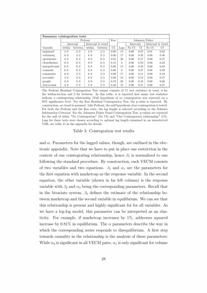
In the next step and based on the unit root test results, cointegrationtests are employed. The results are summarized in table 3. We ruledout the exclusion of individual fixed effects and trends, as it seems tobe an unrealistic assumption from the perspective of the unit root testresults. Note that each variable was tested to be cointegrated with mar-8All variables became stationary when transformed into the first difference form.

26

P-values panel unit root testsNone Intercept Intercept and trend

Variable LLC ADF PP LLC IPS ADF PP LLC Breitung IPS ADF PPmarketcap 1.00 1.00 1.00 1.00 1.00 1.00 1.00 0.79 1.00 0.99 0.99 0.99asquared 0.98 1.00 1.00 0.99 0.99 0.77 0.00 0.86 0.17 0.06 0.00 0.00volumesq 1.00 1.00 1.00 0.99 0.97 0.96 0.03 0.00 0.37 0.00 0.00 0.00openissues 1.00 1.00 1.00 0.06 0.44 0.00 0.00 0.49 1.00 0.11 0.00 0.00closedissues 1.00 1.00 1.00 0.01 1.00 0.01 0.00 0.00 0.98 0.06 0.00 0.00mergedcount 1.00 1.00 1.00 0.00 0.00 0.00 0.00 0.00 1.00 0.00 0.00 0.00commits 1.00 0.00 0.00 0.00 0.00 0.00 0.00 0.00 0.99 0.00 0.00 0.00accounts 1.00 1.00 1.00 1.00 1.00 1.00 1.00 1.00 1.00 0.97 0.52 0.45comments 0.20 0.06 0.00 1.00 0.15 0.01 0.00 0.79 0.81 0.00 0.00 0.00google 0.75 0.90 0.88 0.97 0.59 0.53 0.00 0.02 1.00 0.00 0.00 0.00storycount 0.00 0.00 0.00 0.00 0.00 0.00 0.00 0.00 0.00 0.00 0.00 0.00

The Levin, Lin & Chu (LLC) and Breitung tests have the null hypothesis of a unit root assumingcommon unit root processes, whereas the ADF-Fisher Chi-square (ADF), PP-Fisher Chi-square(PP) and Im, Pesaran and Shin W-stat (IPS) test assume individual unit root root processes. Thetests requiring lag length specification were conducted with lag length selection according to theSchwarz Information Criterion. If the null hypothesis could not be rejected on a 95% significancelevel and the series thus exhibits a unit root, the result in the table is marked in bold.

Table 2: Unit root results

ketcap. Addresses squared, volume squared, comments and accountsshow robust results towards cointegration across tests. Open issues iscointegrated with marketcap if one assumes common AR coefficients forthe underlying tests (referred to as within-dimension) whereas the statis-tics for google show stronger signs for cointegration if individual ARcoefficients are assumed (between-dimension). However, all of these se-ries can be considered cointegrated with marketcap by the majority ofthe test statistics. Again, the aforementioned block consisting of closedis-sues, mergedcount and commits does not show any signs of cointegration,which is in line with the unit root test results, i.e. the series proven tobe stationary are not cointegrated with market cap. The same goes forstorycount, which was stationary across all unit root tests and is notcointegrated with market cap based on the majority of the tests. We willtake a closer look at this variable later.

We move on and estimate the long-run relationship between marketcapand those variables where cointegration was detected in the previous step.For this matter, we leave out closedissues, mergedcount and commits aswe could neither see non-stationarity within the series nor cointegrationwith marketcap. Table 4 reports the estimation results. For the sake of abetter overview, we only show the results for the long-run parameters β

27

Summary cointegration testsPedroni Kao Johansen Fisher

Intercept Intercept & trend Intercept Intercept & trendVariable within between within between CI Lags No CI CI No CI CIasquared 4/8 3/3 4/8 2/3 0.08 15 0.00 0.37 0.01 0.62volumesq 8/8 3/3 8/8 3/3 0.00 17 0.00 0.35 0.00 0.36openissues 4/8 0/3 0/8 0/3 0.05 20 0.00 0.17 0.00 0.37closedissues 0/8 0/3 0/8 0/3 0.15 6 0.00 0.59 0.00 0.23mergedcount 0/8 0/3 0/8 0/3 0.00 15 0.00 0.50 0.00 0.83commits 0/8 0/3 0/8 0/3 0.00 8 0.00 0.37 0.00 0.29comments 6/8 3/3 6/8 3/3 0.00 17 0.00 0.11 0.00 0.19accounts 4/8 3/3 6/8 3/3 0.00 10 0.00 0.13 0.00 0.47google 3/8 3/3 3/8 3/3 0.19 20 0.00 0.10 0.00 0.66storycount 4/8 2/3 5/8 2/3 0.48 12 0.00 0.51 0.00 0.27

The Pedroni Residual Cointegration Test output consists of 11 test statistics in total, 8 forthe within-section and 3 for between. In this table, it is reported how many test statisticsindicate a cointegrating relationship (Null hypothesis of no cointegration was rejected) on a95% significance level. For the Kao Residual Cointegration Test, the p-value is reported. Byconstruction, no trend is assumed. Like Pedroni, the null hypothesis of no cointegration is tested.For both the Pedroni and the Kao tests, the lag lenght is selected according to the SchwarzInformation Criterion. For the Johansen Fisher Panel Cointegration Test, p-values are reportedfor the null of either "No Cointegration" (No CI) and "One Cointegration relationship" (CI).Lags for these tests were chosen according to optimal lag length examined in an unrestrictedVAR, see table 11 in the appendix for details.

Table 3: Cointegration test results

and α. Parameters for the lagged values, though, are outlined in the elec-tronic appendix. Note that we have to put in place one restriction in thecontext of one cointegrating relationship, hence β1 is normalized to onefollowing the standard procedure. By construction, each VECM consistsof two variables and two equations. β1 and α1 are the parameters forthe first equation with marketcap as the response variable. In the secondequation, the other variable (shown in far left column) is the responsevariable with β2 and α2 being the corresponding parameters. Recall thatin the bivariate system, β2 defines the estimate of the relationship be-tween marketcap and the second variable in equilibrium. We can see thatthis relationship is present and highly significant for for all variables. Aswe have a log-log model, this parameter can be interpreted as an elas-ticity. For example, if marketcap increases by 1%, addresses squaredincrease by 0.81% in equilibrium. The α parameters describe the way inwhich the corresponding series responds to disequilibrium. A first steptowards causality in the relationship is the analysis of these parameters:While α2 is significant in all VECM pairs, α1 is only significant for volume

28

squared, accounts and google. In other words, the second variable in thesystem responds in a disequilibrium and adjusts to restore balance. Onthe other hand, marketcap only responds for the three aforementionedcases, whereas for the other variables the same error correction dynamicsare not present. A further illustration of this one-way causality can befound if we restrict α1 to zero and test if this restriction is binding. Forall variables where α1 was insignificant, the null hypothesis of the La-grange Multiplier test result could not be rejected, thus implying weakexogeneity. Put differently, we construct our model such that marketcapcannot be adjusted by the error correction term (α1 = 0) and check ifthis makes a difference compared to the normal model without restric-tion. If it does not, we can state that the marketcap is not affected bythe respective variable in a disequilibrium, which is called weak exogene-ity. This finding will further be confirmed by Granger causality tests, towhich we come back later. First, we employ FMOLS and DOLS estima-tions, as these econometric techniques take into account panel-specificcaveats, opposed to the VECM estimations. While the VECM simplyestimates the stacked data, FMOLS and DOLS allow fixed effects butstill correct for endogeneity and serial correlation in contrast to a simpleOLS regression. Recall that grouped estimation takes the average of eachcross-section and estimates in a second step, whereas pooled estimationremoves cross-section specific components prior to estimation. As onecan see, estimations for asquared, volumesq, comments, accounts andgoogle are quite consistent with the VECM outcomes. In the case ofopenissues, the estimators vary more depending on the underlying as-sumptions, giving a hint that the currencies might be heterogeneous intheir behaviour. This last finding is in line with the fact that the restof the variables in the development factors block are not cointegrated inthe panel context.

Finally, we turn to the panel Granger causality test results. Recall thatone variable Granger causes the other if one adds lagged values of ofthe second variable (besides own past values) and these lags improve theexplanation. For the variables asquared, volumesq, comments, accountsand google, there is strong evidence for a bidirectional Granger causal-

29

Estimation Results long-run relationshipVECM Parameters Weak Exogeneity FMOLS DOLS

Variable β2 α1 α2 yi,t xi,t βPooled βGrouped βPooled βGroupedasquared 0.81*** -0.0003 0.0080*** 0.60 0.00 1.48*** 1.03*** 0.67*** 0.87***

(0.1728) (0.0005) (0.0026) (0.0002) (0.1068) (0.0488) (0.3312)volumesq 0.42*** -0.0056*** 0.0611*** 0.00 0.00 0.43*** 0.39*** 0.33*** 0.35***

(0.0127) (0.0008) (0.0112) (0.0019) (0.0061) (0.0060) (0.0101)openissues 2.09*** -0.0002 0.0009*** 0.43 0.00 5.33*** 4.89*** 1.97*** 4.82

(0.4478) (0.0003) (0.0002) (0.0005) (0.1302) (0.3032) (12.83)comments 2.30*** -0.0003 0.0041*** 0.37 0.00 1.71*** 2.39*** 1.14*** 1.54***

(0.2540) (0.0003) (0.0008) (0.0021) (0.1239) (0.0602) (0.2165)accounts 1.005*** -0.0009** 0.0039*** 0.00 0.00 0.94*** 1.09*** 0.79*** 0.82***

(0.1400) (0.0004) (0.0008) (0.0007) (0.0643) (0.0273) (0.0706)google 2.51*** -0.0007*** 0.0005** 0.00 0.01 1.77*** 3.94*** 1.43*** 2.40***

(0.6732) (0.0002) (0.0002) (0.0004) (0.4573) (0.0552) (0.1439)

All VECM models were first estimated with trend, however, the trend was not significant for any ofthe pair of variables. Thus, trend was excluded for the VECM models as well as for FMOLS andDOLS. In oder to account for heteroskedasticity, pre-withening with lag specification according toAIC were employed for the calculation of the long-run covariance in FMOLS. For DOLS estimation,lags and leads were chosen according to Akaike and the long-run variance pre-whitened as mentionedabove in the pooled case. In the grouped case, the covariance was estimated with HAC (Newey-West)standard errors as well as pre-whitened according to AIC. Stars denote the significance on a 90% (*),95% (**) and 99% (****) significance level.

Table 4: Results Panel VECM, FMOLS and DOLS

ity: Both the stacked test and the Dumitrescu Hurlin results confirmthis on a very high significance level. This is in line with the VECM re-sults, making them more robust. As expected, we see different results forthe development factor block. Openissues clearly exhibits unidirectionalcausality in the sense that marketcap Granger causes openissues but notvice versa, which is confirmed by both tests. In the case of closedissues,we see bidirectional, highly significant causality if we allow the test toconsider individual coefficients. For mergedcount, the same applies onlywith a unidirectional causality if we allow for individual coefficients -here, mergedcount Granger causes marketcap but not vice versa. Theoutcome for commits further confirms the fact that commits might notbe a series which seems to be related to marketcap: We cannot reject thenull that one variable does not Granger causes the other in any case. Fi-nally, storycount shows the expected results of a unidirectional causalityfrom marketcap to storycount, but not vice versa.

Besides estimating the variables on a panel level, we employed the wholemethodology on each currency’s individual level too. As the findings werequite robust for the majority of the variables, we don’t go into detail for

30

Panel Granger Causality Test ResultsStacked test Dumitrescu Hurlin

(Common coefficients) (Individual coefficients)Variable Lags yt xt yt xtasquared 16 0.00 0.00 0.00 0.00volumesq 18 0.00 0.00 0.00 0.00openissues 21 0.63 0.00 0.17 0.00closedissues 7 0.72 0.00 0.00 0.00mergedcount 16 0.45 0.12 0.00 0.42commits 9 0.91 0.27 0.43 0.12comments 18 0.00 0.00 0.00 0.00accounts 11 0.00 0.00 0.00 0.00google 21 0.00 0.00 0.00 0.00storycount 21 0.33 0.00 0.31 0.00

The amount of lags corresponds to the optimal lag length deter-mined for the VECM models + one additional lag. Reported num-bers are p-values for the test "xi,t (the variable listed in the table)does not Granger cause marketcap (yi,t)" for the first column andvice versa for the second column. For the Dumitrescu Hurlin case,the hypothesis is augmented to "xi,t does not homogeneously causeyi,t".

Table 5: Results Granger Causality

the variables where the long-run relationship could be explained on thepanel level. Nevertheless, all estimation outputs are available on thedatabase and within the EViews files. It is interesting, though, to have alook at these variables where a cointegrating relationship was not presentand unit root results would be mixed, namely closedissues, mergedcountand commits. We thus report the VECM results for these in tables 6,7 and 8.9 In the case of closedissues, cointegration is present withinnine currencies. The results show a similar picture to what we have seenin the Panel VECM results: β2 and α2 is significant for all currencies,whereas α1 is not significant exept for Dash, Lisk (lsk), Nem (xem) Nano(xrb). This is again further confirmed by the weak exogeneity tests. Atthis point, we also show the Granger causality tests in order to compareresults with the rest of the estimations. They also confirm the findingsof a rather unidirectional causality: The null of "closedissues (xt) does9Results for unit root and cointegration tests are not reported here, but they areoutlined in the database and EViews files.

31

not Granger cause marketcap (yt)" could not be rejected for almost allcurrencies (Dash is an exception), whereas marketcap Granger causes therespective variable in four cases. If we look at mergedcount, the overallpicture looks the same. Mostly, α2 is significant, with merged count beingweakly exogenous and Granger caused by marketcap, but not vice versa.However, there are a few exceptions as well: For example, in the caseof Litecoin (ltc), there is a unidirectional causality from mergedcountto marketcap, which is confirmed by both weak exogeneity and Grangercausality test. The last variable in the block of development factorswas commits. First of all, this variable seems to have another patterncompared to the other variables, as cointegration was detected for onlyfive currencies. Here, most of the parameters are significant and forStellar (xlm), Ripple (xrp), Verge (xvg) and Monero (xmr), the latteron a 90% significance level and with bidirectional causality accordingto weak exogeneity tests. However, taking into account the Grangercausality test, the finding is put into perspective. Only Verge exhibitsa bidirectional causality, while the other currencies show mixed results.Another variable which was tested on an individual level was storycount.The reason why only three currencies are outlined here is the fact that forother currencies, there was simply not enough data to rely on. Moreover,only those currencies where cointegration is present were estimated. Themethodology was applied to Bitcoin Cash and Ethereum as well.10 Onceagain, we can see that causality seems to be unidirectional: Besides β2being highly significant for all currencies, α2 is the only significant errorcorrection term. Tests for weak exogeneity and Granger causality confirmthis finding.10Only the largest and best-known currencies were tested. In order to compare theoutcomes with a rather small, less-known currency, Zcash was tested as well. How-ever, very little to no stories were published with this keyword. Thus, there was nosense to test this variable for all of the less known currencies.

32

Individual Estimation Results: Closed Issues CountVECM Parameters Weak Exogeneity Granger Causality

Currency Lags β2 α1 α2 yt xt yt xtbtc 6 8.02*** -0.0041 0.0017*** 0.50 0.00 0.47 0.00

(1.2807) (0.0060) (0.0004)dash 6 4.10*** -0.0019*** 0.0012*** 0.00 0.00 0.00 0.00

(0.6407) (0.0006) (0.0004)lsk 0 4.90*** -0.0044** 0.0007*** 0.05 0.00 0.14 0.00

(0.7615) (0.0023) (0.0002)ltc 6 33.93*** 0.0002 0.0004*** 0.68 0.00 0.51 0.44

(6.6117) (0.0004) (0.0001)neo 0 2.45*** 0.0042 0.0046*** 0.37 0.00 0.53 0.47

(0.2703) (0.0047) (0.0008)xem 3 91.55*** -0.0023** 0.00009*** 0.02 0.00 0.99 0.43

(22.66) (0.0009) (0.00002)xmr 6 33.50*** -0.00006 0.0013*** 0.92 0.00 0.08 0.13

(5.78) (0.0005) (0.0013)xrb 2 14.61*** 0.0478*** 0.0025*** 0.00 0.00 0.43 0.00

(2.06) (0.0109) (0.0006)xvg 1 0.81** 0.0027 0.0027*** 0.32 0.00 0.27 0.10

(0.3676) (0.0027) (0.0006)

Cointegration test results are not reported in this table, however, they are outlined inthe database delivered together with this thesis. Lags were determined according toAIC, SC and HQ Information Criterion. The model was estimated with trend, if thetrend component is significant. Granger Causality tests were employed with lag length inVECM + one lag. Stars denote the significance on a 90% (*), 95% (**) and 99% (****)significance level.

Table 6: Results Closed Issues Count

33

Individual Estimation Results: Merged CountVECM Parameters Weak Exogeneity Granger Causality

Currency Lags β2 α1 α2 yt xt yt xtdash 8 0.87* -0.0024*** 0.0010*** 0.00 0.00 0.09 0.00

(0.5056) (0.0008) (0.0002)eos 1 0.80 -0.0110** 0.0072*** 0.04 0.00 0.04 0.00

(0.7589) (0.0050) (0.0013)ltc 1 4.79*** -0.0055*** -0.0002 0.00 0.14 0.01 0.80

(0.6445) (0.0015) (0.0001)neo 2 3.87*** 0.0056 0.0036*** 0.24 0.00 0.09 0.44

(0.8890) (0.0042) (0.0008)xem 2 383.68*** -0.0014*** 0.00006*** 0.00 0.00 0.78 0.23

(44.7750) (0.0004) (0.00001)xlm 4 9.23*** -0.0002 0.0020*** 0.87 0.00 0.00 0.00

(1.1328) (0.0012) (0.0003)xmr 6 1.18*** -0.0040 0.0166*** 0.26 0.00 0.00 0.33

(0.0939) (0.0033) (0.0055)xrb 0 4.02*** 0.0220* 0.0124*** 0.09 0.00 0.12 0.00

(0.4084) (0.0131) (0.0024)


Table 7: Results Merged Count

Individual Estimation Results: CommitsVECM Parameters Weak Exogeneity Granger Causality

Currency Lags β2 α1 α2 yt xt yt xteth 1 1.93*** -0.0006* 0.0056*** 0.52 0.00 0.19 0.00

(0.5315) (0.0009) (0.0016)xlm 4 3.54*** -0.0033*** 0.0015*** 0.00 0.19 0.00 0.57

(0.7436) (0.0008) (0.0010)xmr 1 4.00*** -0.0012* 0.0007*** 0.09 0.00 0.34 0.00

(0.3557) (0.0007) (0.0001)xrp 2 8.46*** 0.0011** -0.0045*** 0.03 0.00 0.58 0.09

(1.5345) (0.0005) (0.0009)xvg 2 2.99*** 0.0056*** 0.0060*** 0.00 0.00 0.01 0.02

(0.5559) (0.0016) (0.0015)


Table 8: Results Commits

34

Individual Estimation Results: StorycountVECM Parameters Weak Exogeneity Granger Causality

Currency Lags β2 α1 α2 yt xt yt xtbtc 5 0.74*** -0.0040 0.5965*** 0.30 0.00 0.23 0.02

(0.0469) (0.0037) (0.0675)ltc 5 4.03*** -0.0022 0.0414*** 0.45 0.00 0.59 0.06

(0.7015) (0.0022) (0.0092)xmr 7 5.43*** -0.0007 0.0325*** 0.75 0.00 0.46 0.35

(0.9232) (0.0018) (0.0061)


Table 9: Results Storycount

4 Discussion

In this thesis, we have estimated the relationship between cryptocurrencyprices and different variables by using a set of panel data consisting of17 cryptocurrencies. Our contribution is to examine Altcoins in a broadand empirical way, as academic literature mostly focussed on Bitcoin upto this date. This may be due to the fact that Bitcoin played a predom-inant role for many years since its appearance in 2008. However, as thedominance of Bitcoin decreased gradually in the past years, the questionof what the determinants for the price of a cryptocurrency are is justi-fied. Since supply is mostly predefined by the source code, we focussedon the demand side. We tested different factors which could play a roleaccording to existing literature.

First, we tested the validity of Metcalfe’s Law by using uniqe addressessquared as proxy and could confirm the findings of Alabi (2017) while ex-tending it to more cryptocurrencies. In the long term, addresses squaredincrease by 0.82% if marketcap increases by 1% if estimated with a panelVECM. However, if we look at the short-term dynamics and causality,our results suggest that addresses squared respond to shocks of market-cap, but not vice versa. If we take daily volume squared as proxy variable,our results show that volume squared increases by 0.42% if marketcap

35

increases by 1%. In this case, the causality is bidirectional, hence bothrespond variables react to a disequilibrium. The findings of were veryrobust, as they are in line with results from estimations using FMOLSand DOLS. Panel Granger causality tests suggested that both series areGranger causing one another no matter if we assume common or individ-ual coefficents, which further confirms that there is a strong link betweenthe series.

Based on the ideas of White (2015), S. Wang and Vergne (2017) andLansky (2016), we tested if there is a relationship between the under-lying technology of a cryptocurrency and marketcap. In order to dothis, we used four proxies based on metrics from GitHub, the majorhosting service for cryptocurrency software projects. Our results showthat cryptocurrencies are quite heterogeneous when it comes to devel-opers activity. First of all, only one variable, openissues, proved to becointegrated with markecap on a panel level. The same conclusion aswith addresses squared can be drawn: It is openissues which responds toshocks in marketcap, but not vice versa. This is confirmed by both weakexogeneity and Granger causality tests. Thus, we might draw the con-clusion that if marketcap increases, programmers have more incentivesto scrutinize the source code and suggest improvements to the core team.The rest of the proxies were not cointegrated with marketcap on the panellevel. This is why we tested each currency individually, employing thesame econometric methodology. For closedissues, nine cryptocurrenciesproved to have a long-run relationship with marketcap. Dash, xem, xrband lsk (the latter on a 90% significance level) exhibit a bidirectionalcausality within the VECM, while the other currencies behave the sameway as openissues, i.e. the causality flows from marketcap to closedis-sues. Mergedcount looks similar, for eight currencies cointegration withmarketcap is present. It is also dash, xem and xrb (the latter on a90% significance level) which show bidrectional causality in VECM, andadditionally eos. For the rest of the currencies, mergedcount is unidirec-tionaly caused by marketcap. An Exception is ltc, where the results arethe other way round. The last variable, commits, has even less currencies

36

with proof of cointegration and mixed results. From these outcomes, wecan clearly see that is rather heterogeneous response behaviour when itcomes to developers activity. However, for the majority of the currencies,some sort of long-run equilibrium could be observed. The mixed resultsare most certainly due to the fact that "technology" and "innovation"are very difficult to measure. It cannot be qualified whether one commitis more valuable than another, and most importantly, the cryptocurren-cies are in different periods of their R&D life-cycle. While Bitcoin hasbeen in place for many years, currencies such as eos or xrb exist since2017. In the early stage, a contribution might be of much more valuecompared to a minor contribution (which is measured as to be equal) inthe Bitcoin source code after many years of existence. Thus, results havecertainly to be qualified on an individual level and it’s probably not agood idea to compare them amongst each other (which is in line withour heterogeneous results). All in all, we observe a tendency towardsmore significant results for older currencies. Hence, it could also be thecase that for younger currencies, there is simply not enough data to drawreliable results from, or, most probably, innovation is not measured wellenough with the present variables. S. Wang and Vergne (2017) used sim-ilar variables to measure innovation potential in their paper and cameto the conclusion that the proxy is positively correlated with weekly re-turns of the cryptocurrency’s price for a panel of five cryptocurrencies(Bitcoin, Litecoin, Ripple, Stellar and Peercoin - the latter was not usedin our analysis). These findings are in line with our results, however, theauthors use a panel regression model and thus, the directions of causalitycould not be fully exploited. In our VECM model, which uses simulta-neous equations, we were able to extend these results and found thatthe causality flows from marketcap towards the proxy measuring innova-tion potential, but not vice versa for the majority of the cryptocurrencies.

Within the community factors, we have a clearer picture on the panellevel. There is a long-run equilibrium between marketcap and com-ments, which is characterized by a unidirectional causality from mar-ketcap to comments. Granger causality tests, however, suggest a bidirec-

37

tional causality. The first finding of comments being weakly exogenouscould be explained by the fact that large movements in price tend tolead to more discussions in the reddit forum. When we look at accounts,causality is bidirectional for all estimation outcomes. If we put this into aMetcalfe’s Law perspective, this makes sense: One could argue that red-dit users interested in the underlying cryptocurrency might also investin it. Thus, a rising number of accounts might be a proxy for adoption.Furthermore, an account corresponds to an individual opposed to uniqueaddresses, where an individual potentially has more than one addresses(Recall that our variable only considers active reddit acounts, thus mak-ing it difficult due to its activity-based property). Alas, it could be thecase that some currencies even use bots to automatically create discus-sion within a forum.

Lastly, we used google search queries as proxy for public interest or in-vestors sentiment, which was often included in models for explaining theBitcoin price. Our results are in line with findings by e.g. Kristoufek(2013). All results prove a bidirectional causality. The constructionproblem of the standardized google search index mentioned in the datasection could certainly be mitigated by the fact that in late 2017, therewas a very strong price rally which was accompanied by enormous publicinterest. It still would be interesting to see absolute measures of searchqueries and compare them for example with other time periods. Be-sides google search queries, we looked at a new variable which was, toour knowledge, never considered in research as a proxy for search enginequeries. As search queries within the Bloomberg terminal might be morerelated to professional investors (whereas google covers mainstream), thiscould lead to more reliable results if we want to measure investors senti-ment. First of all, it has to be mentioned that data is very rare for themajority of the cryptocurrencies discussed in this paper, which certainlyproves that this asset class does not seem to be a broadly discussed topicwithin the investors press. However, cointegration is present for Bit-coin, Litecoin and Monero. Opposed to google search queries, causalityis unidirectional. It seems that more articles are written about a cryp-

38

tocurrency once there is an increase in marketcap. However, Grangercausality results confirm this finding only for btc (on a 95% significancelevel) and ltc (on a 90% significance level).

Within our empirical analysis, we could show the nature of the relation-ships between a cryptocurrency price and its potential determinants. Weextended existing literature insofar to include more cryptocurrencies anda larger time span, as well as by exploiting the direction of causality flows.It is the case quite frequently that marketcap is causing the explanatoryvariable, but not vice versa. This could give a hint that demand factorshave not yet been examined enough. Furthermore, in face of the extremeprice rally in late 2017, it could be the case that increasing prices createdan incentive to develop innovations within the cryptocurrency market.For future research, it might be interesting to go into more details whenit comes to measuring innovation potential and its influence on / rela-tionship with the price of a cryptocurrency. From the estimations for thetime series both on a panel level and each cryptocurrency’s individuallevel, we created a broad database of results which might be used for thisresearch.

39

References

Alabi, Ken (2017). “Digital blockchain networks appear to be followingMetcalfe’s Law”. In: Electronic Commerce Research and Applications24, pp. 23–29.

BitInfoCharts (2018). Number of unique (from or to) addresses per day.https://bitinfocharts.com/comparison/activeaddresses-btc-

eth-bch-ltc-xrp-etc-dash.html. Accessed: March 2018.Bouoiyour, Jamal and Refk Selmi (2015). “What does Bitcoin look like?”In: Annals of Economics & Finance 16.2.

Ciaian, Pavel, Miroslava Rajcaniova, and d’Artis Kancs (2016). “Theeconomics of BitCoin price formation”. In: Applied Economics 48.19,pp. 1799–1815.

Coase, Ronald H (1972). “Durability and monopoly”. In: The Journal ofLaw and Economics 15.1, pp. 143–149.

CoinCheckup.com (2018). Cryptocurrency Pump & Dump information.https://pumpdump.coincheckup.com/. Accessed: May 2018.

CoinMarketCap (2018a). Frequently Asked Questions. https://coinmarketcap.com/faq/. Accessed: May 2018.

– (2018b). Main page. https://coinmarketcap.com/all/views/all/.Accessed: May 2018.

– (2018c). Percentage of Total Market Capitalization (Dominance). https://coinmarketcap.com/charts/#dominance-percentage. Accessed:May 2018.

Dumitrescu, Elena-Ivona and Christophe Hurlin (2012). “Testing for Grangernon-causality in heterogeneous panels”. In: Economic Modelling 29.4,pp. 1450–1460.

Engle, Robert F and Clive WJ Granger (1987). “Co-integration and errorcorrection: representation, estimation, and testing”. In: Econometrica:journal of the Econometric Society, pp. 251–276.

EViews (2018a). Panel Unit Root Testing. http://www.eviews.com/help/helpintro.html#page/content/advtimeser-Panel_Unit_

Root_Testing.html. Accessed: May 2018.

i

https://bitinfocharts.com/comparison/activeaddresses-btc-eth-bch-ltc-xrp-etc-dash.html

https://bitinfocharts.com/comparison/activeaddresses-btc-eth-bch-ltc-xrp-etc-dash.html

https://pumpdump.coincheckup.com/

https://coinmarketcap.com/faq/

https://coinmarketcap.com/faq/

https://coinmarketcap.com/all/views/all/

https://coinmarketcap.com/charts/#dominance-percentage

https://coinmarketcap.com/charts/#dominance-percentage

http://www.eviews.com/help/helpintro.html#page/content/advtimeser-Panel_Unit_Root_Testing.html



EViews (2018b).User’s Guide. http://www.eviews.com/help/helpintro.html#page/content/preface.html. Accessed: May 2018.

Farell, Ryan (2015). “An analysis of the cryptocurrency industry”. In:Granger, Clive WJ (1969). “Investigating causal relations by econometricmodels and cross-spectral methods”. In: Econometrica: Journal of theEconometric Society, pp. 424–438.

Hayek, Friedrich August (1976). “The Denationalisation of Money”. In:The Institute of Economics Affairs, Londres.

ISITC (2016). Annual ISITC Survey Reveals Financial Industry Focuson Disruptive Technology. https://www.isitc.org/news/press-releases/annual-isitc-survey-reveals-financial-industry-

focus-on-disruptive-technology. Accessed: June 2018.Johansen, Søren (1991). “Estimation and hypothesis testing of cointegra-tion vectors in Gaussian vector autoregressive models”. In: Economet-rica: Journal of the Econometric Society, pp. 1551–1580.

– (1995). “Identifying restrictions of linear equations with applications tosimultaneous equations and cointegration”. In: Journal of econometrics69.1, pp. 111–132.

Johnson, Mark (2018). What Is A Pull Request? http://oss-watch.

ac.uk/resources/pullrequest. Accessed: March 2018.Kao, Chihwa (1999). “Spurious regression and residual-based tests forcointegration in panel data”. In: Journal of econometrics 90.1, pp. 1–44.

Kao, Chihwa and Min-Hsien Chiang (2001). “On the estimation and in-ference of a cointegrated regression in panel data”. In: Nonstationarypanels, panel cointegration, and dynamic panels. Emerald Group Pub-lishing Limited, pp. 179–222.

Kao, Chihwa, Min-Hsien Chiang, and Bangtian Chen (1999). “Interna-tional R&D spillovers: an application of estimation and inference inpanel cointegration”. In: Oxford Bulletin of Economics and statistics61.S1, pp. 691–709.

Kristoufek, Ladislav (2013). “BitCoin meets Google Trends andWikipedia:Quantifying the relationship between phenomena of the Internet era”.In: Scientific reports 3, p. 3415.

ii

http://www.eviews.com/help/helpintro.html#page/content/preface.html

http://www.eviews.com/help/helpintro.html#page/content/preface.html

https://www.isitc.org/news/press-releases/annual-isitc-survey-reveals-financial-industry-focus-on-disruptive-technology



http://oss-watch.ac.uk/resources/pullrequest

http://oss-watch.ac.uk/resources/pullrequest

Kristoufek, Ladislav (2015). “What are the main drivers of the Bitcoinprice? Evidence from wavelet coherence analysis”. In: PloS one 10.4,e0123923.

Lansky, Jan et al. (2016). “Analysis of Cryptocurrencies Price Develop-ment”. In: Acta Informatica Pragensia 5.2, pp. 118–137.

Lütkepohl, Helmut and Markus Krätzig (2004).Applied time series econo-metrics. Cambridge university press.

Maddala, Gangadharrao S and Shaowen Wu (1999). “A comparativestudy of unit root tests with panel data and a new simple test”. In:Oxford Bulletin of Economics and statistics 61.S1, pp. 631–652.

Mark, Nelson C and Donggyu Sul (2003). “Cointegration vector estima-tion by panel DOLS and long-run money demand”. In: Oxford Bulletinof Economics and statistics 65.5, pp. 655–680.

Merriam-Webster (2018). Definition of Cryptocurrency. https://www.merriam-webster.com/dictionary/cryptocurrency. Accessed: June2018.

Metcalfe, Bob (2013). “Metcalfe’s law after 40 years of ethernet”. In:Computer 46.12, pp. 26–31.

Nakamoto, Satoshi (2008). Bitcoin: A peer-to-peer electronic cash system.https://bitcoin.org/bitcoin.pdf. Accessed: May 2018.

Ong, Bobby et al. (2015). “Evaluating the potential of alternative cryp-tocurrencies”. In: Handbook of digital currency. Elsevier, pp. 81–135.

Pantula, Sastry G (1989). “Testing for unit roots in time series data”. In:Econometric Theory 5.2, pp. 256–271.

Pedroni, Peter (2001a). “Fully modified OLS for heterogeneous cointe-grated panels”. In: Nonstationary panels, panel cointegration, and dy-namic panels. Emerald Group Publishing Limited, pp. 93–130.

– (2001b). “Purchasing power parity tests in cointegrated panels”. In:Review of Economics and Statistics 83.4, pp. 727–731.

– (2004). “Panel cointegration: asymptotic and finite sample propertiesof pooled time series tests with an application to the PPP hypothesis”.In: Econometric theory 20.3, pp. 597–625.

iii

https://www.merriam-webster.com/dictionary/cryptocurrency

https://www.merriam-webster.com/dictionary/cryptocurrency

https://bitcoin.org/bitcoin.pdf

Phillips, Peter CB and Bruce E Hansen (1990). “Statistical inference ininstrumental variables regression with I (1) processes”. In: The Reviewof Economic Studies 57.1, pp. 99–125.

Phillips, Peter CB and Hyungsik R Moon (1999). “Linear regression limittheory for nonstationary panel data”. In: Econometrica 67.5, pp. 1057–1111.

Smith, Jacob (2016). “An analysis of Bitcoin exchange rates”. In:Stock, James H and Mark W Watson (1993). “A simple estimator ofcointegrating vectors in higher order integrated systems”. In: Econo-metrica: Journal of the Econometric Society, pp. 783–820.

Taub, Bart (1985). “Private fiat money with many suppliers”. In: Journalof Monetary Economics 16.2, pp. 195–208.

Vockathaler, Brian (2015). “The Bitcoin Boom: An In Depth Analysis OfThe Price Of Bitcoins”. In:

Wang, Junpeng, Y Xue, and M Liu (2016). “An Analysis of Bitcoin PriceBased on VEC Model”. In: Proceedings of the 2016 International Con-ference on Economics and Management Innovations.

Wang, Sha and Jean-Philippe Vergne (2017). “Buzz Factor or InnovationPotential: What Explains Cryptocurrencies’ Returns?” In: PloS one12.1, e0169556.

White, Lawrence H (1989). “What kinds of monetary institutions woulda free market deliver”. In: Cato J. 9, p. 367.

– (2015). “The market for cryptocurrencies”. In: Cato J. 35, p. 383.Wooldridge, Jeffrey M (2015). Introductory econometrics: A modern ap-proach. Nelson Education.

iv

Appendix

All results outlined in the paper as well as intermediate results are handedin electronically together with this thesis.

Summary statistics>30% p & d share time period

btc - - - Jun 14 - Jan 18bch 7 3 43% Aug 17 - Jan 18dash 7 2 29% Jun 14 - Jan 18eos 5 2 40% Jul 17 - Jan 18etc 6 5 83% Jul 16 - Jan 18eth 5 3 60% Aug 15 - Jan 18iot 6 0 0% Jun 17 - Jan 18lsk 5 2 40% May 16 - Jan 18ltc 8 1 13% Jun 14 - Jan 18neo 17 3 18% Oct 16 - Jan 18xem 15 3 20% Apr 15 - Jan 18xlm 20 7 35% Aug 14 - Jan 18xmr 8 2 25% Jun 14 - Jan 18xrb 17 4 24% Jul 17 - Jan 18xrp 14 2 14% Jul 14 - Jan 18xvg 83 47 57% Dez 14 - Jan 18zec 6 1 17% Nov 16 - Jan 18

The first column shows the number of times the market cap increased by at least 30%, whereas the secondand third column show how often this was qualified as pump & dump case both as absolute number andpercentage of 30%-spikes. If market cap depreciated by at least 20% up to 5 days following the 30%-increase,it is qualified a pump & dump case. Lastly, the underlying time period is outlined.

Table 10: Evaluation of pump & dump cases across currencies

v

Optimal lag lengthVariable AIC SC HQ Choice

asquared 30 7 15 15volumesq 30 7 21 17openissues 29 15 27 20closedissues 24 2 2 6mergedcount 24 7 20 15commits 29 2 4 8comments 29 7 18 17accounts 27 3 7 10google 30 26 26 20storycount 18 5 18 12In order to determine the optimal lag length, an unrestricted bivariateVAR was estimated, each including marketcap and one of the variablesoutlined in this table. 30 lags were included in order to determine theoptimal lag length. For the final choice of the VECM lags, a middleway of the three information criterions is chosen while making sureto include enough lags to account for possible autocorrelation of theresiduals. One lag length is deducted for the cointegration test and theVECM, since we are running these models in the first difference.

Table 11: Lag length determination

vi

master’s thesis the price of cryptocurrencies: an

Documents