masterÕs thesis - connecting repositories · 5.1.4 calculation behind cerberus ... it verifies...
TRANSCRIPT

0
Faculty of Science and Technology
MASTER’S THESIS
Study program/ Specialization: Petroleum Technology/Drilling
Spring semester, 2014
Open
Writer: Snorre Løge
…………………………………………
(Writer’s signature) Faculty supervisor: Prof. Bernt Sigve Aadnøy External supervisor(s): Sigmund Stokka (IRIS) Thesis title: Review of Completion Technologies Credits (ECTS): 30 Key words: Completion Horizontal wells Buckling Traction tool
Pages: 78 + enclosure: 0
Stavanger, 12.06/2014 Date/year
Figure 1:

i

Abstract
It used to be that completion expenditures were a modest proportion of the total capital costs and field
development time. Today the wells have become exponentially challenging along with new field devel-
opment discoveries. Completion can therefore account for half of total time and cost.
Table 1: Summary of well construction time
Operation: Hours used: Percent time:
36 in. hole 32 3.3
26 in. hole 49 5
Running BOP 39 4
17,5 in. hole 93 9.5
12,25 in. hole 156 15.9
Wellhead 55 5.6
8,5 in. hole 197 20
Lower completion 126 12.8
Upper completion 136 13.9
Start Well 98 10
Total hours: 981 (40,9 days) 100%
(Aadnøy, 2010)
Table 1 shows that completion account for over 50% of the total time spent on constructing a well
(completion effectively starts when drilling 8 1/2" inch hole). In deeper waters additional time is spent
on retrieving/running liners/screens and tripping in/out of the hole.
A majority of the wells planned and constructed today on the Norwegian Continental Shelf (NCS) fall
under horizontal wells category. Horizontal wells, especially shallow wells, are more prone to buckling
and lock-up during completion. Different completion techniques to overcome horizontal related prob-
lems will be studied in this thesis, with emphasis on what is commonly used on the NCS.
Chapter 1 focuses on the different completion methods regularly used and how and why they are
selected.
Chapter 2 goes into sand screens and control of sand production.

ii
Chapter 3 presents buckling theory and the associated challenges.
Chapter 4 presents well tractors and the general use they have in operations today.
Chapter 5 presents the simulation software utilized for running simulations in chapter 6 and the the-
ory behind the program.
Chapter 6 introduces the traction tool concept from IRIS. A Simulation is run to show the traction
tools potential. The chapter ends with experiments done by PhD Terje Moen, re kolibomac project 1995.

iii
Acknowledgments
I would like to thank my partner and children for having such patience with me while writing this thesis.
I would like to thank Sigmund Stokka at IRIS for insightful discussions on the traction tool. Also
thanks to National Oilwell Varco for letting me use their software Cerberus. I am also grateful for all the
help that many people in the industry has provided to me by taking time off from their work day to assist
me with this thesis.
Lastly I would like to thank my adviser, Bernt Sigve Aadnøy, for guiding me down the right path and
for his insightful feedback. It is difficult to visualize how the thesis would have turned out without his
guidance.

Contents
1 Completion 2
1.1 Introduction . . . . . . . . . . . . . . . . . . . . . . . . . . . . . . . . . . . . . . . . . . . . . . . . 2
1.2 Types of Completions . . . . . . . . . . . . . . . . . . . . . . . . . . . . . . . . . . . . . . . . . . 3
1.3 Choosing Completions . . . . . . . . . . . . . . . . . . . . . . . . . . . . . . . . . . . . . . . . . . 4
1.3.1 Open Hole Completion . . . . . . . . . . . . . . . . . . . . . . . . . . . . . . . . . . . . . 4
1.3.2 Pre-drilled or pre-slotted liners . . . . . . . . . . . . . . . . . . . . . . . . . . . . . . . . . 4
1.4 State of Art . . . . . . . . . . . . . . . . . . . . . . . . . . . . . . . . . . . . . . . . . . . . . . . . . 6
1.4.1 Choosing Well Screen . . . . . . . . . . . . . . . . . . . . . . . . . . . . . . . . . . . . . . 6
1.5 Characterize the Reservoir Sand (A) . . . . . . . . . . . . . . . . . . . . . . . . . . . . . . . . . . 6
1.5.1 Particle Size Analysis . . . . . . . . . . . . . . . . . . . . . . . . . . . . . . . . . . . . . . . 8
1.6 Assess Sand Control Options (B) . . . . . . . . . . . . . . . . . . . . . . . . . . . . . . . . . . . . 11
1.7 Specify Filter Media . . . . . . . . . . . . . . . . . . . . . . . . . . . . . . . . . . . . . . . . . . . . 12
1.7.1 Sand Retention Testing . . . . . . . . . . . . . . . . . . . . . . . . . . . . . . . . . . . . . . 12
1.7.2 Pressure-Buildup Data . . . . . . . . . . . . . . . . . . . . . . . . . . . . . . . . . . . . . . 14
1.7.3 Sand Retention data . . . . . . . . . . . . . . . . . . . . . . . . . . . . . . . . . . . . . . . 15
1.8 Refine Sand-Control Selection . . . . . . . . . . . . . . . . . . . . . . . . . . . . . . . . . . . . . 16
1.9 Consider Completion Design . . . . . . . . . . . . . . . . . . . . . . . . . . . . . . . . . . . . . . 17
1.9.1 The Well Path . . . . . . . . . . . . . . . . . . . . . . . . . . . . . . . . . . . . . . . . . . . 17
1.9.2 Reservoir Geomechanics . . . . . . . . . . . . . . . . . . . . . . . . . . . . . . . . . . . . 17
1.9.3 Fluids Program . . . . . . . . . . . . . . . . . . . . . . . . . . . . . . . . . . . . . . . . . . 17
1.9.4 Erosion Potential . . . . . . . . . . . . . . . . . . . . . . . . . . . . . . . . . . . . . . . . . 18
1.9.5 Corrosion Potential . . . . . . . . . . . . . . . . . . . . . . . . . . . . . . . . . . . . . . . . 19
1.9.6 Reservoir Management . . . . . . . . . . . . . . . . . . . . . . . . . . . . . . . . . . . . . 19
1.10 Reducing friction and increasing reachability . . . . . . . . . . . . . . . . . . . . . . . . . . . . 20
iv

CONTENTS v
1.10.1 LoTORQ . . . . . . . . . . . . . . . . . . . . . . . . . . . . . . . . . . . . . . . . . . . . . . 20
2 Sand Control 22
2.1 Sand Production Prediction . . . . . . . . . . . . . . . . . . . . . . . . . . . . . . . . . . . . . . . 22
2.2 Rock Strength . . . . . . . . . . . . . . . . . . . . . . . . . . . . . . . . . . . . . . . . . . . . . . . 22
2.3 Sand Control Screen Types . . . . . . . . . . . . . . . . . . . . . . . . . . . . . . . . . . . . . . . 23
2.4 Wire-wrapped screens . . . . . . . . . . . . . . . . . . . . . . . . . . . . . . . . . . . . . . . . . . 24
2.5 Premium screens . . . . . . . . . . . . . . . . . . . . . . . . . . . . . . . . . . . . . . . . . . . . . 25
2.6 Pre-packed screens . . . . . . . . . . . . . . . . . . . . . . . . . . . . . . . . . . . . . . . . . . . . 27
3 Buckling 28
3.1 Introduction . . . . . . . . . . . . . . . . . . . . . . . . . . . . . . . . . . . . . . . . . . . . . . . . 28
3.2 Tubing-to-casing drag . . . . . . . . . . . . . . . . . . . . . . . . . . . . . . . . . . . . . . . . . . 35
4 Tractor 40
4.1 Introduction . . . . . . . . . . . . . . . . . . . . . . . . . . . . . . . . . . . . . . . . . . . . . . . . 40
4.1.1 Technology . . . . . . . . . . . . . . . . . . . . . . . . . . . . . . . . . . . . . . . . . . . . 40
4.1.2 Hydraulic Well Tractor . . . . . . . . . . . . . . . . . . . . . . . . . . . . . . . . . . . . . . 41
4.1.3 Electric Well Tractor . . . . . . . . . . . . . . . . . . . . . . . . . . . . . . . . . . . . . . . 42
4.1.4 Usage Today . . . . . . . . . . . . . . . . . . . . . . . . . . . . . . . . . . . . . . . . . . . . 42
5 Cerberus 43
5.1 About Cerberus . . . . . . . . . . . . . . . . . . . . . . . . . . . . . . . . . . . . . . . . . . . . . . 43
5.1.1 Overview . . . . . . . . . . . . . . . . . . . . . . . . . . . . . . . . . . . . . . . . . . . . . . 44
5.1.2 Wizard . . . . . . . . . . . . . . . . . . . . . . . . . . . . . . . . . . . . . . . . . . . . . . . 45
5.1.3 Orpheus . . . . . . . . . . . . . . . . . . . . . . . . . . . . . . . . . . . . . . . . . . . . . . 45
5.1.4 Calculation behind Cerberus . . . . . . . . . . . . . . . . . . . . . . . . . . . . . . . . . . 47
6 Traction Tool Concept 52
6.1 Introduction . . . . . . . . . . . . . . . . . . . . . . . . . . . . . . . . . . . . . . . . . . . . . . . . 52
6.2 Technology Background . . . . . . . . . . . . . . . . . . . . . . . . . . . . . . . . . . . . . . . . . 53
6.3 Benefits . . . . . . . . . . . . . . . . . . . . . . . . . . . . . . . . . . . . . . . . . . . . . . . . . . . 54
6.4 Status Today . . . . . . . . . . . . . . . . . . . . . . . . . . . . . . . . . . . . . . . . . . . . . . . . 55
6.4.1 Project Management . . . . . . . . . . . . . . . . . . . . . . . . . . . . . . . . . . . . . . . 56
6.4.2 Prototype Specification & Design . . . . . . . . . . . . . . . . . . . . . . . . . . . . . . . . 56

vi CONTENTS
6.4.3 Detailed Engineering . . . . . . . . . . . . . . . . . . . . . . . . . . . . . . . . . . . . . . . 57
6.4.4 Manufacturing, Assembly and Test . . . . . . . . . . . . . . . . . . . . . . . . . . . . . . 57
6.4.5 Full-scale Qualification . . . . . . . . . . . . . . . . . . . . . . . . . . . . . . . . . . . . . 57
6.5 Simulation . . . . . . . . . . . . . . . . . . . . . . . . . . . . . . . . . . . . . . . . . . . . . . . . . 58
6.6 Experiments by Terje Moen . . . . . . . . . . . . . . . . . . . . . . . . . . . . . . . . . . . . . . . 60
6.6.1 Conclusion of the Kolibomac Project . . . . . . . . . . . . . . . . . . . . . . . . . . . . . 63
7 Conclusion 64
8 Acronyms 66
Bibliography 68

List of Figures
1 . . . . . . . . . . . . . . . . . . . . . . . . . . . . . . . . . . . . . . . . . . . . . . . . . . . . . . . . 0
1.1 Economic influence of completions . . . . . . . . . . . . . . . . . . . . . . . . . . . . . . . . . . 2
1.2 Reservoir completions methods . . . . . . . . . . . . . . . . . . . . . . . . . . . . . . . . . . . . 3
1.3 External Casing Packer . . . . . . . . . . . . . . . . . . . . . . . . . . . . . . . . . . . . . . . . . . 5
1.4 Whole-Core Samples . . . . . . . . . . . . . . . . . . . . . . . . . . . . . . . . . . . . . . . . . . . 7
1.5 Sidewall-Core Samples . . . . . . . . . . . . . . . . . . . . . . . . . . . . . . . . . . . . . . . . . . 7
1.6 Produced-Sand or Bailed-Sand Sample . . . . . . . . . . . . . . . . . . . . . . . . . . . . . . . . 8
1.7 Dry Sieve Process . . . . . . . . . . . . . . . . . . . . . . . . . . . . . . . . . . . . . . . . . . . . . 9
1.8 Laser Diffraction Process . . . . . . . . . . . . . . . . . . . . . . . . . . . . . . . . . . . . . . . . 10
1.9 Dry sieved vs. Laser Diffraction . . . . . . . . . . . . . . . . . . . . . . . . . . . . . . . . . . . . . 11
1.10 Uniformity Coefficient Examples . . . . . . . . . . . . . . . . . . . . . . . . . . . . . . . . . . . . 11
1.11 Screen Selector Aid . . . . . . . . . . . . . . . . . . . . . . . . . . . . . . . . . . . . . . . . . . . . 12
1.12 Slurry Test . . . . . . . . . . . . . . . . . . . . . . . . . . . . . . . . . . . . . . . . . . . . . . . . . 13
1.13 Sand-Pack Test . . . . . . . . . . . . . . . . . . . . . . . . . . . . . . . . . . . . . . . . . . . . . . 14
1.14 Example Plots . . . . . . . . . . . . . . . . . . . . . . . . . . . . . . . . . . . . . . . . . . . . . . . 15
1.15 Example plots . . . . . . . . . . . . . . . . . . . . . . . . . . . . . . . . . . . . . . . . . . . . . . . 15
1.16 Example plots . . . . . . . . . . . . . . . . . . . . . . . . . . . . . . . . . . . . . . . . . . . . . . . 16
1.17 Screen selection . . . . . . . . . . . . . . . . . . . . . . . . . . . . . . . . . . . . . . . . . . . . . . 16
1.18 Example Plots . . . . . . . . . . . . . . . . . . . . . . . . . . . . . . . . . . . . . . . . . . . . . . . 17
1.19 Example plots . . . . . . . . . . . . . . . . . . . . . . . . . . . . . . . . . . . . . . . . . . . . . . . 18
1.20 The variation in erosion rate with particle size as measured in screen erosion testing. . . . . . 19
1.21 Output from inflow performance modeling software . . . . . . . . . . . . . . . . . . . . . . . . 20
2.1 Quartz overgrowth in sandstone . . . . . . . . . . . . . . . . . . . . . . . . . . . . . . . . . . . . 23
vii
LIST OF FIGURES 1
2.2 wire-wrapped screen . . . . . . . . . . . . . . . . . . . . . . . . . . . . . . . . . . . . . . . . . . . 24
2.3 Examples of wire-wrapped screen inflow area(Bellarby, 2009) . . . . . . . . . . . . . . . . . . . 25
2.4 Typical premium screen construction . . . . . . . . . . . . . . . . . . . . . . . . . . . . . . . . . 26
2.5 Example of premium screen . . . . . . . . . . . . . . . . . . . . . . . . . . . . . . . . . . . . . . . 26
2.6 Pre-packed screen(Bellarby, 2009) . . . . . . . . . . . . . . . . . . . . . . . . . . . . . . . . . . . 27
3.1 Buckling caused by internal pressure. . . . . . . . . . . . . . . . . . . . . . . . . . . . . . . . . . 29
3.2 True axial load versus effective axial load . . . . . . . . . . . . . . . . . . . . . . . . . . . . . . . 30
3.3 Finite element analysis of buckling . . . . . . . . . . . . . . . . . . . . . . . . . . . . . . . . . . . 33
3.4 Tubing-to-casing friction . . . . . . . . . . . . . . . . . . . . . . . . . . . . . . . . . . . . . . . . 36
3.5 Tubing-to-casing contact forces in a deviated well . . . . . . . . . . . . . . . . . . . . . . . . . . 37
3.6 Hook load vs. time during a wellbore clean-out . . . . . . . . . . . . . . . . . . . . . . . . . . . 39
4.1 Typical design for a well tractor . . . . . . . . . . . . . . . . . . . . . . . . . . . . . . . . . . . . . 41
5.1 Cerberus software display . . . . . . . . . . . . . . . . . . . . . . . . . . . . . . . . . . . . . . . . 44
5.2 Orpheus’ wizard . . . . . . . . . . . . . . . . . . . . . . . . . . . . . . . . . . . . . . . . . . . . . . 46
5.3 Run at depth feature . . . . . . . . . . . . . . . . . . . . . . . . . . . . . . . . . . . . . . . . . . . 46
5.4 Tubing segment in a straight, inclined section of a well . . . . . . . . . . . . . . . . . . . . . . . 47
5.5 Closed ended pipe suspended in a well . . . . . . . . . . . . . . . . . . . . . . . . . . . . . . . . 48
6.1 The Traction Tool . . . . . . . . . . . . . . . . . . . . . . . . . . . . . . . . . . . . . . . . . . . . . 53
6.2 Axial force on packer at start of sliding . . . . . . . . . . . . . . . . . . . . . . . . . . . . . . . . . 54
6.3 Overall project time line in a Gantt chart . . . . . . . . . . . . . . . . . . . . . . . . . . . . . . . 56
6.5 Report from operator . . . . . . . . . . . . . . . . . . . . . . . . . . . . . . . . . . . . . . . . . . . 59
6.4 Surface weight versus depth without traction tool . . . . . . . . . . . . . . . . . . . . . . . . . . 59
6.6 Surface weight versus depth with traction tool . . . . . . . . . . . . . . . . . . . . . . . . . . . . 60
6.7 The traction tool has a hydraulic packer at each end. Packer A is inflated and cylinder A
is pressurized, pushing the piston forward (1 - 2). Cylinder B is simultaneously pushed
forward, ready for packer (B) inflation. (Moen, 1995) . . . . . . . . . . . . . . . . . . . . . . . . 61
6.8 Design of the packer section with relevant measurements . . . . . . . . . . . . . . . . . . . . . 61
6.9 Radius of curvature as a function of length along the packers under various pressures. . . . . 62
6.10 Increase in diameter as a function of pressure (free, 20mm, 5.8mm, locked down). . . . . . . 62

Chapter 1
Completion
1.1 Introduction
The connection between the reservoir and surface, ensuring safe and efficient production, is known as
the completion. Its role is crucial regarding the economics of a field development. When the field is
starting to produce one can see the importance of a successful completion. Figure 1.1 shows how big
economic impact completion can have on a well.
Figure 1.1: Economic influence of completions(Bellarby, 2009)
A poor completion job can result in lower flow rates from reservoir to surface, unnecessary interven-
tion, installation challenges among other problems.
2

1.2. TYPES OF COMPLETIONS 3
1.2 Types of Completions
Completed wells can be injectors or producers. Using completion, one can produce hydrocarbons and
water or inject hydrocarbons, water, steam and waste products such as carbon dioxide. A well can also
serve more than one purpose, e.g. it is possible to combine production and injection by producing
through the tubing while injecting down the annulus.
It is common to divide completions into an upper- and one lower completion. The upper completion
is given as the interface between conduit from reservoir completion to surface equipment, while the
lower completion is the connection between the well and the reservoir.
Figure 1.2: Reservoir completions methods(Bellarby, 2009)
Some of the key decisions in the reservoir completion are (Bellarby, 2009)
• Well trajectory and inclination
• Open hole versus cased hole
• Sand control requirement and type of sand control
• Stimulation (proppant or acid)
• Single or multi-zone (commingled or selective)

4 CHAPTER 1. COMPLETION
1.3 Choosing Completions
The basis for choosing the right completion depends on numerous factors, one of the early indication is
the inflow performance. It verifies the drop in pressure (production-related pressure), from the reservoir
to the rock face of the reservoir completion. By determining the inflow performance for different well
geometries in the reservoir it can determine what completion strategy to be used (e.g. cased hole ver-
sus open hole). It also provides a value comparison of different reservoir completions, e.g. a long open
horizontal well compared to a vertical hydraulically fractured well.
1.3.1 Open Hole Completion
The vast amount of completion techniques provided by the industry is astonishing, however, selected
techniques will be presented that are relevant for the NCS. Two of the more common completion tech-
niques used are pre-drilled-/slotted-liners and screens (screens will be covered in chapter 2) both tech-
niques fall under the term open hole.
1.3.2 Pre-drilled or pre-slotted liners
The aim for this completion technique is to:
• Prevent gross hole collapse.
• Allow for isolation, either advanced or later, by permitting zonal isolation packers to be set up
within the reservoir completion.
• Allow for deployment of intervention tool strings.
This techniques function poorly as sand control because of the difficulty to make the slots small
enough to shut out the sand. Some companies provide laser cut liners with small apertures, but then
a new problem is introduced and the liners become susceptible to plugging. This can be avoided by
combining the liners with SAGD (Steam Assist Gravity Drainage) with coarse sediments and injection to
help prevent plugging.
The pre-drilled liners are commonly favored over pre-slotted liners because of their larger inflow area
and greater strength. These two properties also eliminates the concern for pressure drop through the
holes and plugging. It is possible to change the geometry of the slots in a pre-slotted liner to improve the
overall strength, however, they still perform poorly when compared to the pre-drilled liners — especially
under formation collapse or installation torque loads.

1.3. CHOOSING COMPLETIONS 5
Figure 1.3: External Casing Packer(Bellarby, 2009)
When installing a pre-drilled or pre-slotted liner you can do it with or without a washpipe. Since
sand control is rarely an issue when using liners, they are usually installed in mud. This mitigates the
risk for surge and swab or mechanical abrasion causing disrupt to the filter cake and high losses. When
production is initiated the mud and filter cake is produced through the liner. Thereafter, the washpipe
purpose is then assigned to contingency, in case circulation is required to removed cuttings or other
objects from the front of the liner. The washpipe can at this time also be used to set External Casing
Packers (ECP), displace solutions for removal of the filter cake or closing valves for fluid loss control.
There is a significant disadvantage using an open hole completion technique (expandable solid liners
is an exception to this), trying to achieve zonal isolation. It is possible to perform cement and gel treat-
ments operations through pre-drilled liners, but they have a meager success rate. The more viable option
is to install equipment with the liner. The two methods favored in the industry are swellable elastomer
packers and ECPs, but with an increasingly popularity for mechanical open hole packers.
External Casing Packers
For many years the only method for zonal isolation (liner run into open hole wells) was with the use of
ECPs. Their general structure is shown in Figure 1.3.
The ECPs is selected upon potential isolating horizons (often shale). It is paramount that the liner
reaches its intended depth.

6 CHAPTER 1. COMPLETION
1.4 State of Art
1.4.1 Choosing Well Screen
One of the steps for maximizing and optimizing the recovery of hydrocarbons in a reservoir is by sand
control. There is a vast amount of sand reservoirs with sand of different properties. Produced sand in
your well stream can cripple production, causing considerable complications with flowlines and surface
production equipment. The industry need to have broad knowledge of reservoir sand properties, such as
particle size, particle size distribution (PSD) and particle size uniformity is central to the design of sand
control completions. The choice of well screen based on the sand properties, and other factors, can have
an extensive effect on the productivity and efficiency of a producing well.
What steps to take exactly to acquire the right sand screen for a well is handled different within the
industry. The following is an excerpt from Weatherfords Sand Screen Selector (Weatherford, 2015a).
1.5 Characterize the Reservoir Sand (A)
When using mechanical equipment to control the sand production, the first thing to do is to determine
the size of the formation sand to properly size the filter mechanism. Formation sand must also be evalu-
ated to determine the grain-size distribution.
A sample of the reservoir is required and the sample should be representative of the planned comple-
tion interval. Core samples or data from offset wells can be used, given that there is a high certainty that
they are representative of the sand to be retrieved.
Whole-Core Samples
Representative samples from whole core provides the most accurate information about in-situ grain size
and grain-size distribution.
• All sands present is represented
• The rock fabric is undamaged
• Appropriate samples can be selected

1.5. CHARACTERIZE THE RESERVOIR SAND (A) 7
Figure 1.4: Whole-Core Samples
(who)
Side-Core Samples
Using sidewall core samples is usually acceptable and usually provides a fair understanding. Sand grains
can be shattered during coring which, in turn, can result in in altered grain-size distribution data.
• Discrete locations
• Mud contamination
• Crushed grains
Figure 1.5: Sidewall-Core Samples
(sid)

8 CHAPTER 1. COMPLETION
Produced Sand Samples
Very hard to produce results which is representative of the in-situ grain size and grain-size distribution.
The analysis usually implies an unrealistic amount of fines present.
• Questionable source
• Risk of incomplete distribution
• High ratio of smaller sand grains/fines can distort the screen sizing process.
Bailed-Sand Samples
This method should be used with caution, as bailed samples will usually be skewed toward larger particles
that have not been flowed to surface.
• Uncertain source
• Risk of incomplete distribution
• High ratio of larger sand grains can distort the screen sizing process.
Figure 1.6: Produced-Sand or Bailed-Sand Sample
(pro)
1.5.1 Particle Size Analysis
From the methods available, two methods are more common than the others. Dry sieving and laser
particle sizing (LPSA) is the preferred choice in most circumstances, however, it should be noted that the
result from these two techniques can vary and this should be considered during screen selection.

1.5. CHARACTERIZE THE RESERVOIR SAND (A) 9
Dry Sieving
The sample is cleaned, crushed, dried, weighed and then sorted using a multiple sieves with openings in
accordance to ASTM E11-13(Standard, 2013). The weight of sand in each sieve is recorded, all the way
down to No. 325 mesh (44 µm).
The overall weight percent of each saved sample is then plotted against the the sieve aperture on
semi-log coordinates to achieve a size distribution plot.
• A sample size greater than 10g is required for a representative test
• Its lower measures is according to No. 325 mesh (45 µm)
• A good dispersion can be hard to obtain
Figure 1.7: Dry Sieve Process
(dry)
10 CHAPTER 1. COMPLETION
LPSA
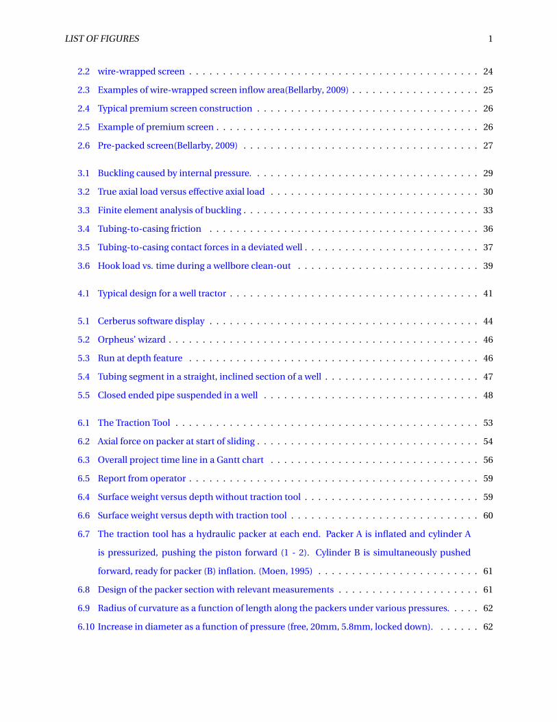
The concept is that the diffraction angle of light striking a particle is inversely proportional to the particle
size. The sand sample is placed inside the unit and the light diffraction caused by all the particles is mea-
sured, in turn concluding the size of individual particles. The unit is integrated with a computer which
allows for an automated process. An analysis software will record and plot the grain-size distribution.
• For a representative test a smaller sand sample is required than dry sieving.
• Can measure down to 4 µm
• The average diameter is measured
Figure 1.8: Laser Diffraction Process
(las)
Grain-Size Distribution
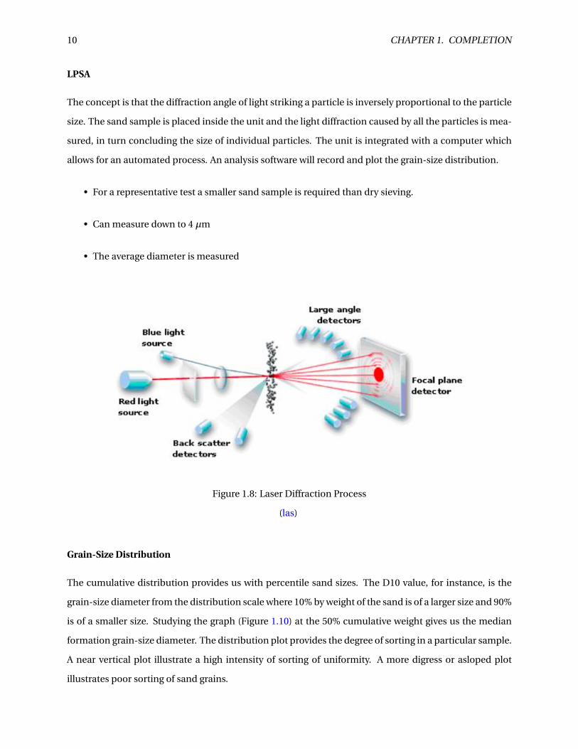
The cumulative distribution provides us with percentile sand sizes. The D10 value, for instance, is the
grain-size diameter from the distribution scale where 10% by weight of the sand is of a larger size and 90%
is of a smaller size. Studying the graph (Figure 1.10) at the 50% cumulative weight gives us the median
formation grain-size diameter. The distribution plot provides the degree of sorting in a particular sample.
A near vertical plot illustrate a high intensity of sorting of uniformity. A more digress or asloped plot
illustrates poor sorting of sand grains.
1.6. ASSESS SAND CONTROL OPTIONS (B) 11
Figure 1.9: Dry sieved vs. Laser Diffraction
(Weatherford, 2015b)
Figure 1.10: Uniformity Coefficient Examples
(Weatherford, 2015b)
1.6 Assess Sand Control Options (B)
The measured PSD provides the basis for selecting the optimal methods to control a predetermined sand
or assortment of sands. Using the grain size and sorting of the finest sand likely to fail and produced solids
can tell what type of screen should be implemented (Figure 1.11). For coarse, well-sorted sand, WWS is
suitable, slotted liners (SL) is also a viable option. Encountering more poorly sorted sands and/or the
fines content increases, metal-mesh screens (MMS) and openhole gravel pack (OHGP) are more practical
solutions.

12 CHAPTER 1. COMPLETION
Figure 1.11: Screen Selector Aid
(Weatherford, 2015b)
1.7 Specify Filter Media
To confirm the screen recommendation a sand retention test can be applied. The optimal filter media
and aperture size is determined by testing each sand with wire-wrap or metal-mesh filters, applying both
slurry and sand-pack test methods.
1.7.1 Sand Retention Testing
Slurry Test
Slurry tests simulate open-annulus/non-compliant borehole conditions. Slurry with suspended sand is
directed through a screen. The end result is the weight of solids produced through the screen and the rate
of pressure buildup across the screen versus the amount of sand contacting the screen.

1.7. SPECIFY FILTER MEDIA 13
Figure 1.12: Slurry Test
(Weatherford, 2015b)
Sand-Pack Test
Sand-pack tests simulate compliant sand control or a collapsed borehole. The sand is situated directly
onto the screen, a wetting liquid is then flowed through the sand-pack and screen. From this test the
amount of sand passing through is derived through weight, as well as the differential pressure.
14 CHAPTER 1. COMPLETION
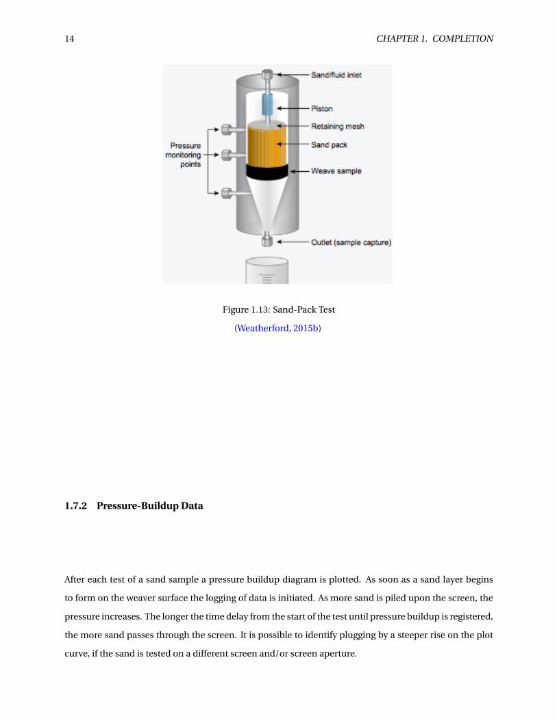
Figure 1.13: Sand-Pack Test
(Weatherford, 2015b)
1.7.2 Pressure-Buildup Data
After each test of a sand sample a pressure buildup diagram is plotted. As soon as a sand layer begins
to form on the weaver surface the logging of data is initiated. As more sand is piled upon the screen, the
pressure increases. The longer the time delay from the start of the test until pressure buildup is registered,
the more sand passes through the screen. It is possible to identify plugging by a steeper rise on the plot
curve, if the sand is tested on a different screen and/or screen aperture.
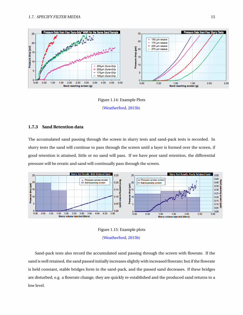
1.7. SPECIFY FILTER MEDIA 15
Figure 1.14: Example Plots
(Weatherford, 2015b)
1.7.3 Sand Retention data
The accumulated sand passing through the screen in slurry tests and sand-pack tests is recorded. In
slurry tests the sand will continue to pass through the screen until a layer is formed over the screen, if
good retention is attained, little or no sand will pass. If we have poor sand retention, the differential
pressure will be erratic and sand will continually pass through the screen.
Figure 1.15: Example plots
(Weatherford, 2015b)
Sand-pack tests also record the accumulated sand passing through the screen with flowrate. If the
sand is well retained, the sand passed initially increases slightly with increased flowrate; but if the flowrate
is held constant, stable bridges form in the sand-pack, and the passed sand decreases. If these bridges
are disturbed, e.g. a flowrate change, they are quickly re-established and the produced sand returns to a
low level.

16 CHAPTER 1. COMPLETION
Figure 1.16: Example plots
(Weatherford, 2015b)
1.8 Refine Sand-Control Selection
When the appropriate filer media is determined, a distinct screen selection and sand-control method can
be refined. The goal of selecting the most pertinent sand-control method is the proficiency to minimize
sand production while lowering the impact on well productivity.
Figure 1.17: Screen selection
(Weatherford, 2015b)
1.9. CONSIDER COMPLETION DESIGN 17
1.9 Consider Completion Design
For any given reservoir, there may be numerous applicable sand-control options. Comprehensive com-
pletion engineering establish the most applicable of all possible options.
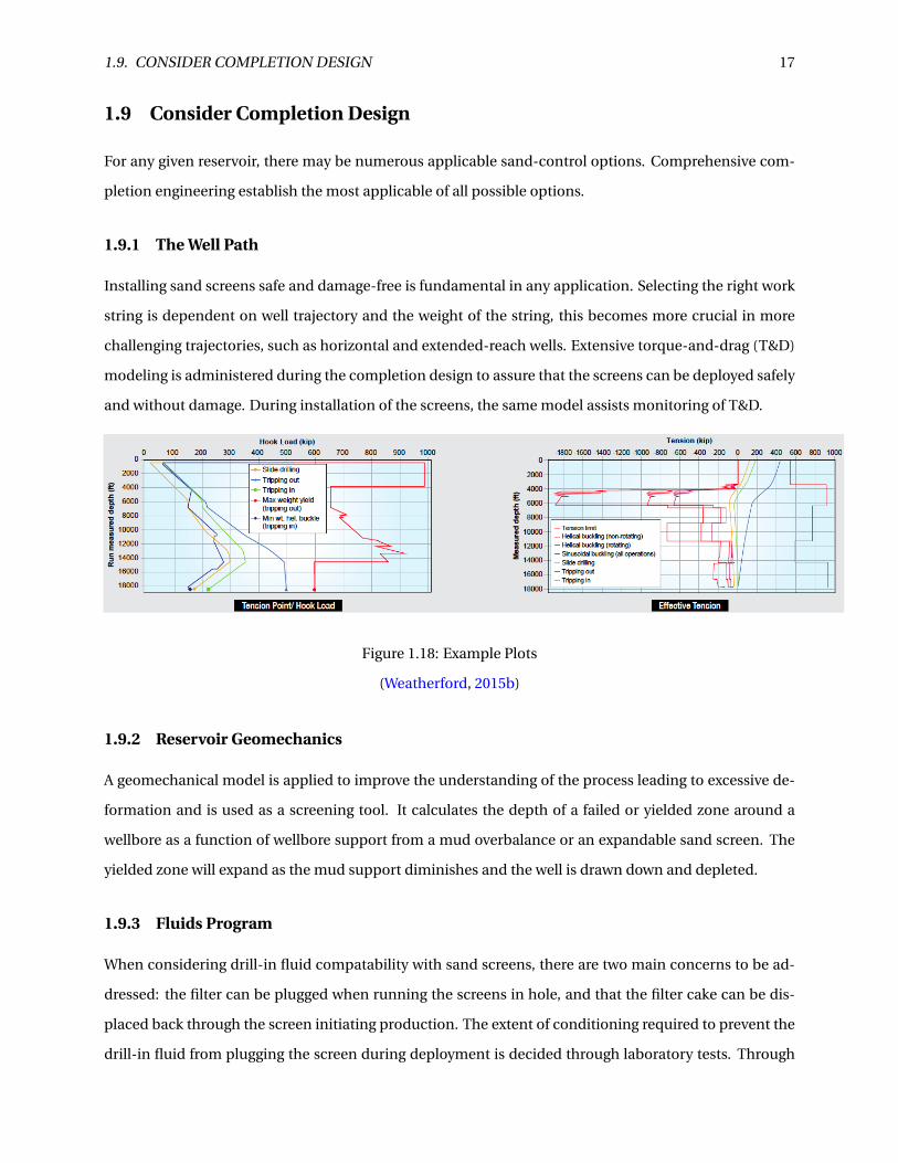
1.9.1 The Well Path
Installing sand screens safe and damage-free is fundamental in any application. Selecting the right work
string is dependent on well trajectory and the weight of the string, this becomes more crucial in more
challenging trajectories, such as horizontal and extended-reach wells. Extensive torque-and-drag (T&D)
modeling is administered during the completion design to assure that the screens can be deployed safely
and without damage. During installation of the screens, the same model assists monitoring of T&D.
Figure 1.18: Example Plots
(Weatherford, 2015b)
1.9.2 Reservoir Geomechanics
A geomechanical model is applied to improve the understanding of the process leading to excessive de-
formation and is used as a screening tool. It calculates the depth of a failed or yielded zone around a
wellbore as a function of wellbore support from a mud overbalance or an expandable sand screen. The
yielded zone will expand as the mud support diminishes and the well is drawn down and depleted.
1.9.3 Fluids Program
When considering drill-in fluid compatability with sand screens, there are two main concerns to be ad-
dressed: the filter can be plugged when running the screens in hole, and that the filter cake can be dis-
placed back through the screen initiating production. The extent of conditioning required to prevent the
drill-in fluid from plugging the screen during deployment is decided through laboratory tests. Through
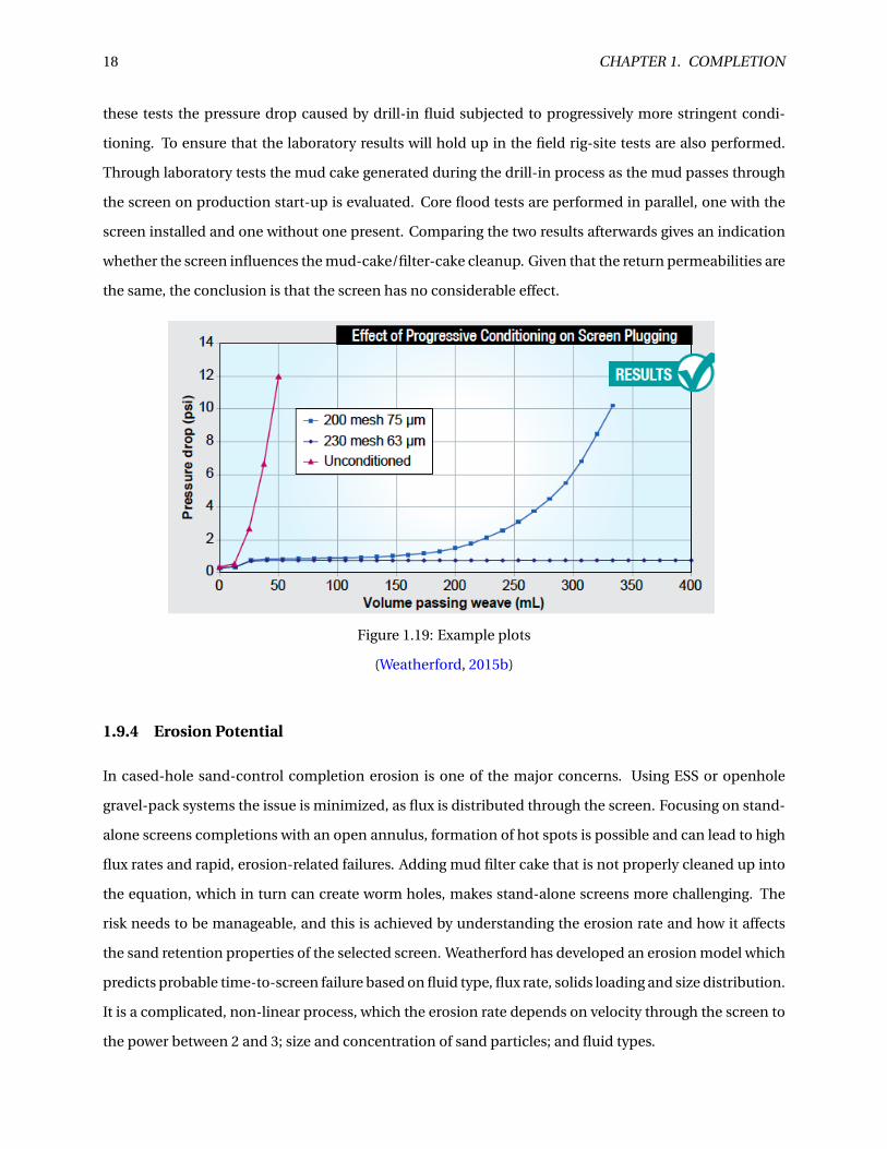
18 CHAPTER 1. COMPLETION
these tests the pressure drop caused by drill-in fluid subjected to progressively more stringent condi-
tioning. To ensure that the laboratory results will hold up in the field rig-site tests are also performed.
Through laboratory tests the mud cake generated during the drill-in process as the mud passes through
the screen on production start-up is evaluated. Core flood tests are performed in parallel, one with the
screen installed and one without one present. Comparing the two results afterwards gives an indication
whether the screen influences the mud-cake/filter-cake cleanup. Given that the return permeabilities are
the same, the conclusion is that the screen has no considerable effect.
Figure 1.19: Example plots
(Weatherford, 2015b)
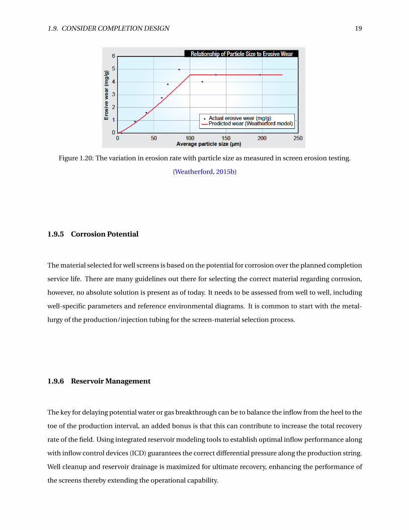
1.9.4 Erosion Potential
In cased-hole sand-control completion erosion is one of the major concerns. Using ESS or openhole
gravel-pack systems the issue is minimized, as flux is distributed through the screen. Focusing on stand-
alone screens completions with an open annulus, formation of hot spots is possible and can lead to high
flux rates and rapid, erosion-related failures. Adding mud filter cake that is not properly cleaned up into
the equation, which in turn can create worm holes, makes stand-alone screens more challenging. The
risk needs to be manageable, and this is achieved by understanding the erosion rate and how it affects
the sand retention properties of the selected screen. Weatherford has developed an erosion model which
predicts probable time-to-screen failure based on fluid type, flux rate, solids loading and size distribution.
It is a complicated, non-linear process, which the erosion rate depends on velocity through the screen to
the power between 2 and 3; size and concentration of sand particles; and fluid types.
1.9. CONSIDER COMPLETION DESIGN 19
Figure 1.20: The variation in erosion rate with particle size as measured in screen erosion testing.
(Weatherford, 2015b)
1.9.5 Corrosion Potential
The material selected for well screens is based on the potential for corrosion over the planned completion
service life. There are many guidelines out there for selecting the correct material regarding corrosion,
however, no absolute solution is present as of today. It needs to be assessed from well to well, including
well-specific parameters and reference environmental diagrams. It is common to start with the metal-
lurgy of the production/injection tubing for the screen-material selection process.
1.9.6 Reservoir Management
The key for delaying potential water or gas breakthrough can be to balance the inflow from the heel to the
toe of the production interval, an added bonus is that this can contribute to increase the total recovery
rate of the field. Using integrated reservoir modeling tools to establish optimal inflow performance along
with inflow control devices (ICD) guarantees the correct differential pressure along the production string.
Well cleanup and reservoir drainage is maximized for ultimate recovery, enhancing the performance of
the screens thereby extending the operational capability.

20 CHAPTER 1. COMPLETION
Figure 1.21: Output from inflow performance modeling software
(Weatherford, 2015b)
1.10 Reducing friction and increasing reachability
1.10.1 LoTORQ
To prevent friction in wells, which reduces the reach in wells, "Weatherford developed the LoTORQ sys-
tem as a centralizer and an axial and rotational friction-reduction system to perform independently of
drilling or completion mud-film strength or lubricity."(lot) It is a one of a kind system, which makes use of
bidirectional rollers, has been tested and used successfully on the world’s most challenging wells. Rollers
that are in contact with the inner pipe can achieve decidedly low friction factors, with rotating coefficients
in cement coming down to 0.04. Rollers with a higher profile which makes contact with the wellbore
wall have consistently reduced axial-friction factors by 60%. The low torque and drag allows for rota-
tion, providing enhanced mud displacement and cement job. With minimal roller-contact in openhole
applications the risk of differential sticking is greatly reduced, providing the user with optimal standoff
and increasing the operational efficiency. The rollers ensures that wear resistance is kept to a minimum
within the life expectancy for the well, allowing casing or tubing retrieval, if necessary. To meet expected
life-time, one of a kind engineering is applied together with correct material selection. This ensures that
shear stresses remain within elastic limits, preventing roller failure.
The LoTORQ makes it achievable to rotate pipe once restricted by torque, providing ideal displace-
ment efficiency and cement sheath. It provides optimal performance in many challenging situations,

1.10. REDUCING FRICTION AND INCREASING REACHABILITY 21
running screen into horizontal and extended-reach wells being one of its key attributes.

Chapter 2
Sand Control
2.1 Sand Production Prediction
It is estimated that approximately 90% of the world’s oil and gas wells are drilled in sandstone reservoirs
(although 60% of the oil and gas reserves are in carbonate reservoirs). (Ian C. Walton, 2001)
Produced sand is unwanted and can lead to loss of integrity, erosion of equipment and, in the worst
case, fatalities. At the same time, choosing not to have sand control can be costly and destructive to
productivity and reservoir management.
Predicting reservoir failure and the production of sand is essential to deciding whether to use down-
hole sand control and what type of sand control to use. The production of sand depends on three main
components(Bellarby, 2009):
1. The strength of the rock and other intrinsic geomechanical properties of the rock
2. Regional stresses imposed on the perforation or wellbore
3. Local loads imposed on the perforation or wellbore due to the presence of the hole, flow, reduced
pore pressures and the presence of water
2.2 Rock Strength
Deposited sediments are, by nature, weak. However, some strength lies within deposited sand. "Cohesion
(friction, granular interlocking and capillary forces) can bind the sand grains together." (Bellarby, 2009) It
is easy to observe the role of capillary forces, trying to build a sandcastle with dry sand instead of damp.
Trying to achieve the same under water seems almost impossible. Compacted irregular grains can show
22

2.3. SAND CONTROL SCREEN TYPES 23
moderate strength, even without cement, by granular interlocking. To create a stronger rock cement is
needed to "bind" the grains together. Pressure exerted by compaction, temperature, and the passage of
water with minerals in solution assists the formation of cement. Silica in the form of quartz overgrowth
is one of the strongest cements, Fig.2.1
Figure 2.1: Quartz overgrowth in sandstone
(Bellarby, 2009)
The mechanisms that tie the grains together will also reduce the pore throats which, in turn, reduces
the permeability and porosity. "The reduction in permeability and porosity and the increase in strength
will depend on the type of cement and its distribution."(Bellarby, 2009)
2.3 Sand Control Screen Types
The industry offers a wide range of screens to choose from. They can be subdivided into three main types:
• Wire-wrapped screens (WWS)
• Premium screens (also known as mesh or woven screens)
• Pre-packed screens (PPS)
All types of screens commercially provided today can be run in either an open hole well or a cased hole
with or without gravel packing. Although this is true, each screen type will have an ideal environment

24 CHAPTER 2. SAND CONTROL
Figure 2.2: wire-wrapped screen(wws)
for which it will perform optimally. The risk of failure while running the screen in an open hole can be
reduced by using a pre-installed, pre-drilled liner. This provides an additional installation protection.
2.4 Wire-wrapped screens
Most commonly used in gravel pack and standalone completions. They are made up of a base pipe with
pre-drilled holes, rods going alongside the pipe and a single wedge-shaped wire wrapped and spot welded
to the rods (see Fig.2.2)
There are those who offer wire-wrapped screen without the longitudinal rods, but they play an impor-
tant role of keeping the offset of the wire wrap from the pre-drilled base pipe holes. The wire is wrapped
helical around the base pipe and is usually welded or fastened with a connector at the ends of the screen.
It can be a challenge to weld the screen to the base, this depends on metallurgy, but can be avoided.
The wire has a keystone shape which allows particles to bridge off against the wire or pass right
through and be produced. The keystone shape makes the WWS, to a degree, self cleaning. However,
the WWS still has a relatively low inflow area. The inflow area is dependent on several properties; wire
thickness, percentage of screen joint that makes up slots (as opposed to the connections) and the slot
width. "Consulting Fig.2.3, using Coberly criteria for slot sizing (2 X D10), the screen inflow areas are cal-
culated for a variety of formation grain sizes and two sizes of wire (0.047 in and 0.09 in.). It is assumed
that 90% of the screen joint length comprises slots."(Bellarby, 2009)
Should, the more conservative, 1 X D10 criteria be used, one would see a decrease in nearly 50% in
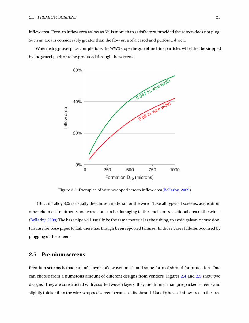
2.5. PREMIUM SCREENS 25
inflow area. Even an inflow area as low as 5% is more than satisfactory, provided the screen does not plug.
Such an area is considerably greater than the flow area of a cased and perforated well.
When using gravel pack completions the WWS stops the gravel and fine particles will either be stopped
by the gravel pack or to be produced through the screens.
Figure 2.3: Examples of wire-wrapped screen inflow area(Bellarby, 2009)
316L and alloy 825 is usually the chosen material for the wire. "Like all types of screens, acidisation,
other chemical treatments and corrosion can be damaging to the small cross-sectional area of the wire."
(Bellarby, 2009) The base pipe will usually be the same material as the tubing, to avoid galvanic corrosion.
It is rare for base pipes to fail, there has though been reported failures. In those cases failures occurred by
plugging of the screen.
2.5 Premium screens
Premium screens is made up of a layers of a woven mesh and some form of shroud for protection. One
can choose from a numerous amount of different designs from vendors, Figures 2.4 and 2.5 show two
designs. They are constructed with assorted woven layers, they are thinner than pre-packed screens and
slightly thicker than the wire-wrapped screen because of its shroud. Usually have a inflow area in the area

26 CHAPTER 2. SAND CONTROL
of 30% and offer some depth filtration, but the porosity of the mesh can exceed 90%.
Figure 2.4: Typical premium screen construction
(Bellarby, 2009)
Figure 2.5: Example of premium screen
(Bellarby, 2009)

2.6. PRE-PACKED SCREENS 27
2.6 Pre-packed screens
These are constructed much the same as to wire-wrapped screens, but instead using two screens. In
between the screens there is gravel packed, usually consolidated as to avoid for a possible void develop-
ment. Some like to see the pre-packed screens as a pre-built gravel pack. However, the gravel pack fills
up the annulus between the screen and formation. In turn preventing sand failure and sand transport.
Pre-packed screens have neither of these functions. Pre-packed screens provides, to an extent, depth
filtration, and with a high porosity (over 30%) in combination with high permeabilities provide mini-
mal pressure drops. The pre-packed screen usage has decreased considerably, replaced by wire-wrapped
screens and premium screens, although they maintain their popularity in some areas of the world.
Figure 2.6: Pre-packed screen(Bellarby, 2009)

Chapter 3
Buckling
3.1 Introduction
Understanding the theory that lies behind buckling is important for everyone involved in well operations.
Buckling can lead to various, undesirable, scenarios:
1. Likely high bending stresses, which in turn lead to low axial (and tri-axial) safety factors as well as
bending loads on connections;
2. Considerable tubing-to-casing contact forces, and if drag is present then this can decrease axial
loads transferring along the tubing;
3. Torque is exerted on connections, which in extreme situations, can unscrew them;
4. The length of the tubing is shortened when buckled - sometimes helpful, usually not;
5. resulting doglegs that can limit through tubing access.
Buckling is identified with structural elements that are thin in comparison to their length. In disci-
plines, such as civil engineering, buckling requires compressional forces (e.g. building a skyscraper). In
the world of oil and gas where tubes are used there is an additional complication due to the presence of
internal and external pressures. This can be demonstrated by envisioning a small section of tubing with
internal pressure (fig.3.1)
28
3.1. INTRODUCTION 29
Figure 3.1: Buckling caused by internal pressure.
(Bellarby, 2009)
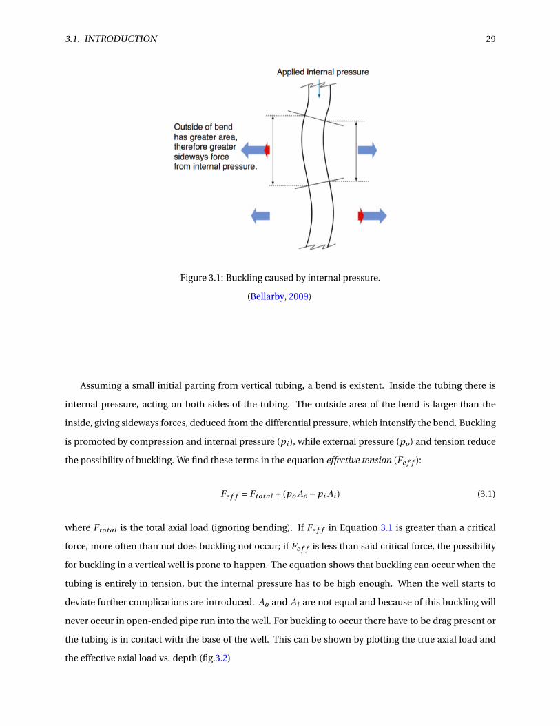
Assuming a small initial parting from vertical tubing, a bend is existent. Inside the tubing there is
internal pressure, acting on both sides of the tubing. The outside area of the bend is larger than the
inside, giving sideways forces, deduced from the differential pressure, which intensify the bend. Buckling
is promoted by compression and internal pressure (pi ), while external pressure (po) and tension reduce
the possibility of buckling. We find these terms in the equation effective tension (Fe f f ):
Fe f f = Ftot al + (po Ao −pi Ai ) (3.1)
where Ftot al is the total axial load (ignoring bending). If Fe f f in Equation 3.1 is greater than a critical
force, more often than not does buckling not occur; if Fe f f is less than said critical force, the possibility
for buckling in a vertical well is prone to happen. The equation shows that buckling can occur when the
tubing is entirely in tension, but the internal pressure has to be high enough. When the well starts to
deviate further complications are introduced. Ao and Ai are not equal and because of this buckling will
never occur in open-ended pipe run into the well. For buckling to occur there have to be drag present or
the tubing is in contact with the base of the well. This can be shown by plotting the true axial load and
the effective axial load vs. depth (fig.3.2)

30 CHAPTER 3. BUCKLING
Figure 3.2: True axial load versus effective axial load
(Bellarby, 2009)
In figure 3.2 it should be noted that the effective axial load goes directly to zero at the base of the
tubing, because buoyancy and the pressure component of the effective axial load are equal in magnitude
and opposite in sign.
Calculating the critical force (Fc ) can be done using Lubinski (Lubinski, 1962). Buckling comes in
two modes, helical or sinusoidal buckling. Sinusoidal buckling is also known as lateral buckling having
an "S" shape, however it is not a true sinusoidal. The term sinusoidal is the more commonly used, and
will consistently be used throughout this thesis. The critical forces for helical and sinusoidal buckling are
given in Equations (3.2) and (3.3).
Helical buckling:
Fc = 4.05(E I w2)1/3 (3.2)
Sinusoidal buckling:
Fc = 1.94(E I w2)1/3 (3.3)
Fc is the critical force measured in pounds (lb), w is the effective, buoyed, weight of the tubing (lb/in.).
The buoyancy is calculated from buoyancy factors or from the pressure-area effect and I the tubing mo-
ment of inertia (in.4).

3.1. INTRODUCTION 31
Table 3.1: Onset of buckling
Condition Meaning
Fe f f <−Fc Tubing will tend to buckleFe f f >−Fc Tubing will not tend to buckle
The moment of inertia (I ) is given by:
I = π
64(D4
o −D4i ) (3.4)
where Do is the tubing outside diameter (in.) and Di is the tubing inside diameter (in.).
It should be noted that there is a divergence in the sign conventions. The critical force is a positive
force but compressive in nature, and compression is usually denoted by a negative axial load. This is
corrected with the definition in Table 3.1.
Tubing with larger diameter and thicker walls will have a more extensive critical force due to the
increased moment of inertia and greater weight. The magnitude of the critical forces is usually small in a
vertical well, a few examples are presented in Table3.2
"In most completions, in a vertical wellbore, there is a narrow window for sinusoidal buckling and to
a first approximation the critical buckling force is zero and helical buckling occurs when Fe f f becomes
negative."(Bellarby, 2009)
The facts that are shown in Equations 3.2 and 3.3 are being somewhat disputed (J. C., 2003). However,
in the vertical case, this is of little practical relevance as the critical buckling forces are usually low.
In a deviated wellbore, the critical buckling force is given by Dawson and Paslay (Dawson and Paslay,
1984) in Equations 3.5 and 3.6.
Sinusoidal buckling:
Fc =√(
4E I w si nθ
rc
)(3.5)
Helical buckling:
Fc = 1.41 ∼ 1.83
√(4E I w si nθ
rc
)(3.6)
where θ is the hole angle and rc is the radial clearance, which is the difference in radius between casing
inner radius and tubing outer radius (in.).
In Equation 3.6 the variation between 1.41 and 1.83 contemplate the uncertainty about the point that
sinusoidal buckling switches to helical buckling (Aasen and Aadnøy, 2002; J. C., 2003). Complications
arise by the fact that the switch from sinusoidal to helical buckling does not occur under the same loads

32 CHAPTER 3. BUCKLING
Table 3.2: Critical force in buckling example
Tubing outside diameter (OD) (in.) 3.5 in. 7 in.Weight (lb/ft) 9.2 32
Tubing inside diameter (ID) (in.) 2.992 in. 6.094 in.Effective weight (with seawater) (lb/in.) 0.66 2.31
Moment of inertia (in.4) 3.43 50.2Fc (sinusoidal) (lb) 693 3887
Fc (helical) (lb) 1446 8115
Table 3.3: Buckling example - inclined well
Tubing OD (in.) 3.5 in. 7 in.Casing ID (in.) 6.184 8.681
Radial clearance (in.) 1.342 0.840Fc (sinusoidal) at 45◦ (lb) 12,011 10,8203
Fc (helical) at 45◦ (lb) 16,935-21,979 152,566-198,011Fc (sinusoidal) at 90◦ (lb) 14,283 128,676
Fc (helical) at 90◦ (lb) 20,139-26,138 181,432-235,476
as the switch back from helical to sinusoidal buckling. The situation is further complicated when entering
curved wellbores and with connections.
Given the examples in Table 3.2, the critical buckling forces at 45◦ and 90◦ are calculated (Table 3.3).
It should be remarked that the larger radial clearance and the smaller 3.5 in. tubing form a much
lower critical buckling force. At the same time, the critical forces are now decidedly higher than they were
for a vertical well. There is a slight simplification in the formulas as the tubing is assumed as infinite and
the axial component of the weight is ignored. As a result of this the critical buckling force is calculated
to zero for a vertical well. In a deviated well the tubing has to overcome gravity by being lifted off the
low side of the well for buckling to occur. At first, sinusoidal buckling will take place changing to helical
buckling once the tubing rises half way up the walls of the casing.
Buckling in a curved wellbore gets more complicated, which introduces a correction for the bending
and contact load of tubing following a curved wellbore (X. and A., 1995). The analysis up to this point
have left out essential elements, friction will be discussed in section 3.4. The upsets on the outside of
the pipe will be discussed now, namely connections. This is a complex problem and can be approached
two ways. Mitchell is one who actively promotes the analytically understanding to the problem (Mithell,
2001)(Mitchell and Miska, 2004). The other option is to use finite element analysis (FEA), but with both
the analytically and FEA approach new issues arise. The tubing is partly centralized by the connections
which limits surface contact of tubing with casing. If the buckling forces are low and/or centralization

3.1. INTRODUCTION 33
significant, the tubing may not contact casing anywhere apart from at tubing connections, but simply
sag towards the casing in a sinusoidal fashion. Upset pipe will induce buckling at an earlier stage than
for smooth pipe. It is more likely that contact will happen away from the connections and modified
sinusoidal- or helical buckling.
Figure 3.3: Finite element analysis of buckling
(Bellarby, 2009)
Figure 3.3 shows an example of the use of FEA for analyzing the partial centralization effect of tubing
connections. It shows the radial midpoint of three joints of tubing. The concentric circles is an illustration
of how far the midpoints can move laterally. Away from the connections, tubing can have contact with
casing. At the connections, it is restrained by the reduced radial clearance. The boundary conditions are
no movement or rotation in any direction at the packer and no lateral movement at the point the load is
applied. It is important to include the connectors in the analysis because they can simultaneously cause
higher than expected loads away from the connection, but reduced bending loads on the connection
itself. Therefore the connection loads will have to include an analysis of the bending component, without
this level of detail they can be overestimated.(Bellarby, 2009)
34 CHAPTER 3. BUCKLING
In other engineering disciplines, buckling is considered an disastrous event and is averted. Well en-
gineering tolerates buckling somewhat more than the other disciplines. It is limited by contact of the
tubular with either the casing or formation, therefore some degree of buckling can be tolerated. The
pitch of the buckled tube and the radial clearance directly affect the severity of buckling. With sinusoidal
buckling, the maximum λ (helix angle) needs to be calculated because it is not constant through the ’S’
shape. Entering helical buckling the λ will be constant (ignoring connections and end effects). (R. F.,
1996) gives the maximum helix angle (λmax ) with an approximate solution.
Sinusoidal buckling:
λmax = 1.1227p2E I
F 0.04e f f (Fe f f −Fc )0.46 (3.7)
Helical buckling:
λ=√
Fe f f
2E I(3.8)
The helix angle (λ) relates directly to the pitch (P):
P = 2π
λ(3.9)
The resulting dogleg is calculated as:
DLS = 68,755rcλ2 (3.10)
where DLS is the dogleg severity (◦/100 ft).
The 68,755 comes from the conversion of radians per inch into degrees per 100 feet.
An effect of these doglegs is bending stress (calculated by equation ??) and, should the bending stress
exceed the yield stress of the pipe, the pipe will permanently corkscrew.
If torque is exerted onto the drill pipe it can promote buckling. This also work the other way, if helical
buckling occurs torque is also induced. Mitchell ?? gives us a detailed presentation of his torque analysis:
τ=± Fe f f r 2c β
2√
1− r 2c β
2(3.11)
where:
β=√
−Fe f f
2E I(3.12)
The unit for torque (τ) is punched in as in.lb in these equations, but are easily converted to ft.lb by
diving by 12.

3.2. TUBING-TO-CASING DRAG 35
Generally, buckling-induced torque is often not taken serious due to the low torque it produces; how-
ever, if the tubing has a small diameter or the radial clearance is considerable, then the torque can be
large in comparison to the make-up torque for the connections. The torque can be defined as either
negative or positive depending on the (random) selection of clockwise or anticlockwise helix.
For a 3.5 in., 9.2 lb/ft, L80, New Wam connection (minimum make-up torque 2930 fl lb) (Bellarby,
2009), as an example, there is little risk for the connections to unscrew, but when dealing with non-
premium connections and low grade material there is always a small risk involved.
Other than creating torque and bending stresses, buckling also alters (reduces) the length of the tub-
ing. The buckling strain (εb) aids in determining the length changes (length change caused by buckling
per unit length). The buckling strain is a function of the radial clearance and the helix angle. When enter-
ing sinusoidal buckling computing the buckling strain can be challenging, because the helix angle does
not remain constant throughout the sinusoidal and therefore an average is required.
Sinusoidal buckling:
εb =−0.7285r 2
c
4E IF 0.08
e f f (Fe f f −Fc )0.92 (3.13)
Helical buckling:
εb =− r 2c
4E IFe f f (3.14)
Integrating these equations will provide an estimate of the total change in length over the length of
the well. This needs to account for the length change due to the buckling itself changing the axial load
and therefore the effective tension.
3.2 Tubing-to-casing drag
Drag opposes tubing movement and transfers axial loads to the casing.
Usually when considering completions, drag is often considered of secondary importance. There is
however some situations where drag plays a crucial role. Problems are sometimes encountered when
running the lower completion. This can happen when running a sand screen into high-angle wells, es-
pecially where the well fluid is less lubricating than the original drilling mud and rotating the pipe is
prevented by damage considerations.
Consulting Figure 3.4, it shows the components of drag.

36 CHAPTER 3. BUCKLING
Figure 3.4: Tubing-to-casing friction
(Bellarby, 2009)
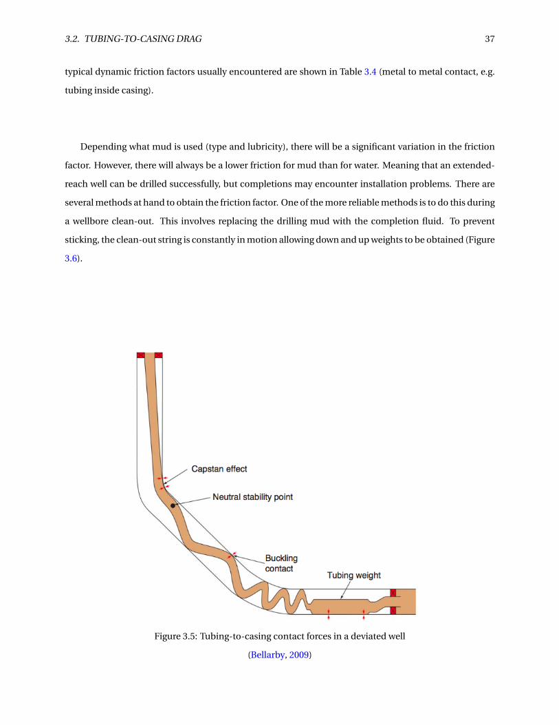
The contact force (Fn) between the tubing and casing dervies from three main sources:
• Forces due to gravity: For a deviated well there will be a component of the tubing weight that will act
onto the casing. When running tubing into a horizontal well, all of the buoyed weight is transferred.
• Forces from buckling: Buckling will not occur unless there is contact with the casing. The severity
of buckling is directly linked to the contact force (e.g. high buckling = larger contact force).
• Forces due to the capstan effect: This force is created due to the fact that the tubing passes through
doglegs. When the tubing is in tension it is pulled into the inside of the bend and a contact force is
generated. When the tube experience compression loads the opposite will occur.
All of the described effects can occur in a single load case as shown in Figure 3.5
The friction factor (µ) is just a part of the contact force that is established in the drag load. Where a
zero friction factor signifies no friction. Drag is either static or dynamic in nature, and static being higher
of the two. The job, in this case, is to install lower completion and static drag is often ignored. What
3.2. TUBING-TO-CASING DRAG 37
typical dynamic friction factors usually encountered are shown in Table 3.4 (metal to metal contact, e.g.
tubing inside casing).
Depending what mud is used (type and lubricity), there will be a significant variation in the friction
factor. However, there will always be a lower friction for mud than for water. Meaning that an extended-
reach well can be drilled successfully, but completions may encounter installation problems. There are
several methods at hand to obtain the friction factor. One of the more reliable methods is to do this during
a wellbore clean-out. This involves replacing the drilling mud with the completion fluid. To prevent
sticking, the clean-out string is constantly in motion allowing down and up weights to be obtained (Figure
3.6).
Figure 3.5: Tubing-to-casing contact forces in a deviated well
(Bellarby, 2009)
38 CHAPTER 3. BUCKLING
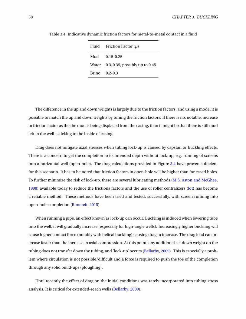
Table 3.4: Indicative dynamic friction factors for metal-to-metal contact in a fluid
Fluid Friction Factor (µ)
Mud 0.15-0.25
Water 0.3-0.35, possibly up to 0.45
Brine 0.2-0.3
The difference in the up and down weights is largely due to the friction factors, and using a model it is
possible to match the up and down weights by tuning the friction factors. If there is no, notable, increase
in friction factor as the the mud is being displaced from the casing, than it might be that there is still mud
left in the well - sticking to the inside of casing.
Drag does not mitigate axial stresses when tubing lock-up is caused by capstan or buckling effects.
There is a concern to get the completion to its intended depth without lock-up, e.g. running of screens
into a horizontal well (open-hole). The drag calculations provided in Figure 3.4 have proven sufficient
for this scenario. It has to be noted that friction factors in open-hole will be higher than for cased holes.
To further minimize the risk of lock-up, there are several lubricating methods (M.S. Aston and McGhee,
1998) available today to reduce the frictions factors and the use of roller centralizers (lot) has become
a reliable method. These methods have been tried and tested, successfully, with screen running into
open-hole completion (Rimereit, 2015).
When running a pipe, an effect known as lock-up can occur. Buckling is induced when lowering tube
into the well, it will gradually increase (especially for high-angle wells). Increasingly higher buckling will
cause higher contact force (notably with helical buckling) causing drag to increase. The drag load can in-
crease faster than the increase in axial compression. At this point, any additional set down weight on the
tubing does not transfer down the tubing, and ’lock-up’ occurs (Bellarby, 2009). This is especially a prob-
lem where circulation is not possible/difficult and a force is required to push the toe of the completion
through any solid build-ups (ploughing).
Until recently the effect of drag on the initial conditions was rarely incorporated into tubing stress
analysis. It is critical for extended-reach wells (Bellarby, 2009).

3.2. TUBING-TO-CASING DRAG 39
Figure 3.6: Hook load vs. time during a wellbore clean-out
(Bellarby, 2009)

Chapter 4
Tractor
4.1 Introduction
Well tractors were introduced to the industry to counter the high operational costs for servicing horizon-
tal wells. It is a cost effective alternative when compared to the highly expensive and time consuming
conventional drill pipe operations. A conventional well tractor can pull coiled tubing/wireline into a
horizontal well, while simultaneously pushing tools. It can be used for drilling operations if fitted with
a positive displacement motor and a drill bit. During the drilling operation, the well tractor will apply
exceptional weight on bit, this setup is usually applied to horizontal drilling (side-track holes or vertical
slimhole drilling).
4.1.1 Technology
Initially the well tractor were designed to be used in long horizontal and large deviated extended reach
wells. It is capable of pulling more than 10,000 ft coiled tubing (CT)/wireline (WL) in horizontal wells,
with a record of 20,000 ft (March Haci, 2001), and more than 25,000 ft of CT/WL in a highly deviated well.
Basically two designs with modular constructions are used. One heavy duty well tractor, which can
run CT together with powerful tools, is hydraulically driven. And an electric driven well tractor which is
designed to run WL, providing an option to run at a more cost efficient level.
The hydraulic driven well tractor have a power ratio of 6 to 1, when compared with the electrical
version. Because of the limitations of electrical power transfer through the WL, the electrical well tractor
comes up short. However, this is of little importance since WL operations require far less pulling force
than operations using CT.
40

4.1. INTRODUCTION 41
Table 4.1: Well tractor sizesWell Tractor O.D. (in.) Operating size I.D. (in.)
3 1/8" 3.2" — 7.25"4 3/4" 4.9" — 12"2 1/8" 2.2" — 4.5"
The well tractor comes in a variety of sizes, Table 4.1 lists up the sizes and what hole/tube size they
can be operated in (courtesy of Welltec).
Several traction sections makes up the well tractor, where the sections are designed so that the well
tractor is self centering in the hole. The numbers of sections required is dependent on the power source,
what force is required and the type of operation to be completed. Normally five is required when using
the hydraulic well tractor and the electrical has a minimum requirement of three sections. With the mod-
ular construction the pulling capacity can be modified by adding or removing the number of sections,
however at one point it will be a decision between maximum running speed and pulling capacity.
The sections are driven internally by a sequence system. Activation from topside allows the sequence
to push the rollers from the well tractor body against the casing/completion or open hole walls, providing
a high force to build traction and move forward with CT/WL and attached tools. Reversing the sequence
will retract the spring loaded rollers into the tool, rendering the well tractor totally flush and ready for
extraction.
Figure 4.1: Typical design for a well tractor
(wel)
The well tractor can be configured for reverse running with approximately the same pulling capacity.
4.1.2 Hydraulic Well Tractor
The hydraulic version is powered by fluids (brine/water, mud, acid, etc). The fluid is pumped down
through the CT, flowing through an internal mud motor connected to the well tractor. The fluid then
passes through the body of the well tractor and out in front for maximum hole cleaning capacity. A mini-
mum flow is required for operation, the minimum flow is dependent of the required pulling capacity and

42 CHAPTER 4. TRACTOR
running speed.
Control of the tool is done from the surface by electric signals through the WL, which is integrated in
the CT. The electric cable allows to switch the rollers on/off while pumping and the tractor body is fitted
with an electric connection which makes it possible to attach logging tools in front of the tractor.
There is a configuration without the electric wire through the CT, this allows for higher flow rates or a
smaller size of coiled tubing.
4.1.3 Electric Well Tractor
The electric version is designed to run on all types of standard WL. Power from the surface is supplied
to the tool through the WL. The WL is connected to a power supply box at surface, which is fitted with a
variable speed control system.
The tractor is fitted with electric wires which runs through the tool body. This enables the tractor to
push logging tools and simultaneously transfer the data to the surface through the WL. The tractor is also
fitted with a power/relay system which allows for logging while pulling out of the hole.
4.1.4 Usage Today
Implementing the well tractor to operations will save time and money when compared to conventional
technology. It operates in both cased and open holes and can be used for operations such as:
• Cleaning
• Setting and pulling of plugs
• Operating Sliding sleeves
• Drilling
• Open hole logging
• Running of production logs
• Cement bond logs (CBL)
• Pushing video cameras

Chapter 5
Cerberus
5.1 About Cerberus
Cerberus is a modeling software directed at operations different operations. It was created in 1995 and
it quickly became an indispensable program for numerous service companies and operators worldwide.
The program is a product of NOV CTES, based in Texas and committed to developing innovative model-
ing solutions and supporting the industry with the best technology available. It gives the user different
options for state-of-the-art calculations.
43

44 CHAPTER 5. CERBERUS
Figure 5.1: Cerberus software display
(NOV)
An area that Cerberus excel in is its ability to model conditions in deviated and horizontal wellbores,
making the software an ideal candidate to analyze the problems presented in this thesis. It is the only
commercially available program able to model all three conveyance methods in one package.
5.1.1 Overview
• Models
– Fatigue life (Achilles™)
– Hydraulics (Hydra™)
– Tubing forces (Orpheus™)
• Editors — configuration tools to enter input data required by the models
• Monitors — real-time job modeling at the wellsite, for enhanced safety and efficiency
• Reporting — professional print output, with integrated e-mail for ease of distribution
It can analyze different problems associated with running tools into and out of a well, such as;
5.1. ABOUT CERBERUS 45
• coiled tubing,
• wireline,
• slickline,
• jointed pipe.
As well as accurately predict and analyze cumulative forces and tubing fatigue at each stage of a job. It is
capable of answering questions crucial to a job analysis. Relevant questions to be answered can be:
• Can the target depth be reached?
• Can the desired tasks/operations be performed?
• Can the equipment be returned safely to surface?
5.1.2 Wizard
Cerberus comes with a built-in wizard which guides the user through complex configuration and de-
signer tasks. These tools assist the user through decisive decisions in a logical and intelligent sequence,
producing choices based on context and user’s previous selections. Cerberus wizard make extensive use
of graphics, calculation utilities, and customization to present operation-specific selections.
5.1.3 Orpheus
Orpheus is Cerberus tubing forces model, it calculates the cumulative forces acting on the tubing. It
considers effects such as helical buckling, drag and hydraulic effects, in order to determine the usefulness
of the job and to foresee possible problems with lock-up or yield. The Q&A wizard 5.2 in Orpheus provides
the user with a intuitive interface that quickly answers common questions. It also has the option to
plan ahead, giving the user options if you get stuck toolstring or if the well condition changes during
the operation. To see whether or not you will have a buckled string Orpheus have a feature called ’Run
at Depth’ which lets the user observe if you enter buckling mode while tripping in/out (Figure 5.3). It
models intervention or drilling operations in the wellbore at specific depths, where there are multiple
conveyance methods available.

46 CHAPTER 5. CERBERUS
Figure 5.2: Orpheus’ wizard(NOV)
Figure 5.3: Run at depth feature(NOV)

5.1. ABOUT CERBERUS 47
Figure 5.4: Tubing segment in a straight, inclined section of a well(Ken Newman)
5.1.4 Calculation behind Cerberus
Introduction
Working in the background of Cerberus there are basic force calculations performed on the length of the
tubing. These calculations is performed on segments of the string from bottom up to surface, and the
total is summed together to get the final result. This method can be visualized by an example (5.4). From
Figure 5.4, it shows the decomposition of the weight WS into two component forces. FN is the force which
acts in the normal direction (perpendicular to the axis of the hole) and FA is the force acting along the
axial direction. Giving us the following equations:
FA =WScosθ (5.1)
FN =WS si nθ (5.2)

48 CHAPTER 5. CERBERUS
The friction coefficient in the well is multiplied with the normal weight component (FN ) to derive the
friction force.
FF =µFN (5.3)
Adding together Equation 5.1 and 5.3 produces the real axial force (FR ). The axial component of the
weight lead FR to be in tension, making it a positive force (by definition). However, it is the direction of
the motion that dictates the sign of the force. When you are Running Into Hole (RIH) the friction causes
everything to compress, making it a negative force. When Pulling Out Of Hole (POOH) it the opposite is
true and a positive sign is produced. The following equation is used, respectively for RIH and POOH:
FR = FA ±FF (5.4)
This equation is used as a basis for calculating one segment of tubing. Adding up all the segments of a
tubing string produces the axial force on the tubing in the well along its length. When the ’run at depth/
function is executed this force versus length profile is calculated by Orpheus.
Real versus Effective Force
Many people mix up or misunderstand the concept of real axial force (FR ) and effective force (FE ) (the
latter is sometimes referred to as the ’fictitious force’). To clear things an easy example can be pre-
sented.(Ken Newman)
Figure 5.5: Closed ended pipe suspended in a well
(Ken Newman)
Only the lower part of the tube is considered (from point "A" and downwards). In the figure, ξi is
the density of the fluid inside the pipe (psi/ft) and ξo is the density on the outside of the pipe. The same

5.1. ABOUT CERBERUS 49
terminology applies for Pi and Po , but for pressure instead of density (psi). An equation for the axial force
components can be made with three simple steps:
1. weight of the pipe acting downward =WS X
2. Upward force exerted on the end of pipe due to differential pressure = PoB Ao
3. Downward force exerted on the pipe due to differential pressure = Pi B Ai
Adding these equations yields the real axial force at point A:
FR =WS X +Pi B Ai −PoB Ao (5.5)
Calculating Pi B and PoB :
Pi B = Pi A +X ξi (5.6)
PoB = Po A +X ξo (5.7)
Buoyancy is defined as (weight per foot):
WB =W S +ξi (5.8)
Taking Equation 5.6,5.7,5.8 into Equation 5.5 and after some rearrangements produces the following
equation:
FR =WB X +Pi A Ai −Po A Ao (5.9)
The effective force can now be defined as:
FE = FR −Pi A Ai +Po A Ao (5.10)
It should be noted that Equation 5.10 is a definition and is not to be considered a real physical force.
Comparing Equation 5.9 and 5.10 it is seen that the effective force is the real force, excluding the effects
of pressure included. The effective force is a favorable equation to work with for several reasons. It is now
possible to use the effective force on point A, combining Equation 5.9 and 5.10:
FE =WB X (5.11)
This equation is a much simpler equation to utilize in a tubing forces model than Equation 5.9. The
buckling characteristics of a pipe depend upon effective force instead of real force, making it invaluable

50 CHAPTER 5. CERBERUS
in Cerberus. Buoyancy, independent of depth, is of physical significance and affects buckling; however,
pressure, which is dependent of depth, does not affect buckling. The only consequential quantities that
depend on the real force are strain and stress. Meaning, that the tubing force model works with effec-
tive force calculations. The effective force is only converted to real force for output purposes and stress
calculations.
Stress Calculations
Orpheus utilize two different stress calculations. The von Mises stress calculations is used by default, as it
is advised from CTES. It combines the axial stress due to the force on the tubing combined with the radial
stress caused by internal pressure and hoop stress caused by internal and external pressure. Calculating
the combined stress at the inside surface of the pipe. To calculate the von Mises the real force, FR , has to
be used.
Should the user wish to turn the von Mises calculations off, then Orpheus will only calculate the axial
stress. Which is just the real axial force in the pipe divided by the cross-sectional area. This allows the
user to only see the major component of the total stress by itself.
Underlying Equation
As previously mentioned, Orpheus calculates the string at a given position in the well (the bottom end
of the string). It then calculates the torque and effective force in segments up towards the surface. The
length of one segment is dependent on variations in fluid density, wall thickness, hole diameter, fluid
density inside and outside the pipe and well geometry. The user have the option to change the maximum
segment length, but Orpheus has set to 100 ft by default. The differential equation(Bhalla et al., 1994)
which is integrated over the segment is:
dFE
d s=WB cosθ
dγ
d s+µ
dFN
d scosβ and
dTF
d s= rµ
dFN
d sσ (5.12)
where
dFN
d s=
√(FE si nθ
dγ
d s
)2
+(FE
dθ
d s+WB si nθ
)2
(5.13)
and
σ=
−1, nonzero torque is applied to non-rotating pipe.
si nβ, otherwise.(5.14)
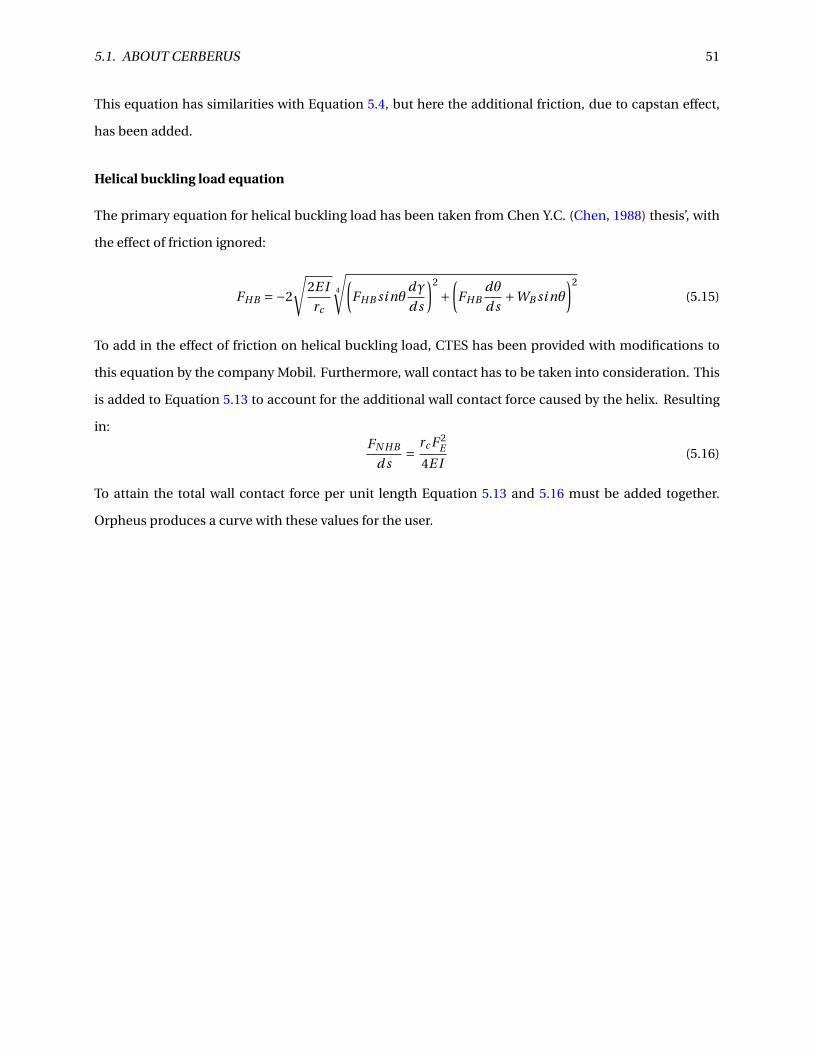
5.1. ABOUT CERBERUS 51
This equation has similarities with Equation 5.4, but here the additional friction, due to capstan effect,
has been added.
Helical buckling load equation
The primary equation for helical buckling load has been taken from Chen Y.C. (Chen, 1988) thesis’, with
the effect of friction ignored:
FHB =−2
√2E I
rc
4
√(FHB si nθ
dγ
d s
)2
+(FHB
dθ
d s+WB si nθ
)2
(5.15)
To add in the effect of friction on helical buckling load, CTES has been provided with modifications to
this equation by the company Mobil. Furthermore, wall contact has to be taken into consideration. This
is added to Equation 5.13 to account for the additional wall contact force caused by the helix. Resulting
in:FN HB
d s= rc F 2
E
4E I(5.16)
To attain the total wall contact force per unit length Equation 5.13 and 5.16 must be added together.
Orpheus produces a curve with these values for the user.

Chapter 6
Traction Tool Concept
6.1 Introduction
The traction tool is a concept that IRIS has developed and is currently being qualified. It is a robust tool
that can provide traction on demand when running liners and sand screens in challenging wellbores. It
is a spin-off from the HOP (Hole in One Producer), a concept which allows for simultaneous drilling and
completion.
It will be used when running liners and sand screens in challenging wellbores to provide a pulling
force when required. Frictional lock-up can be avoided, allowing the completion string to reach its TD
(Target Depth). Failing to reach TD can lead to reduced well production and reduced oil recovery.
With sand screens in particular, if large loads are required during run in hole in order to push the
completion to TD then there is a risk of equipment damage. Sand screen with damage can result in a
sand production problem, which in turn can lead to reduction in well production rate and a costly repair
operation.
Extended reach wells that are planned today are often limited in its length due to the risk of not being
able to install the liner or sand screen. Applying the traction tool to these wells will allow for drainage
further into the reservoir, which in turn gives improved recovery.
52

6.2. TECHNOLOGY BACKGROUND 53
Figure 6.1: The Traction Tool
Consulting Figure 6.1, it displays the traction tool in operation, assisting the running of a liner or sand
screen into an 81/2 inch diameter borehole. The traction tool is mounted on the end of the completion
string and is powered by mud circulation. With the aid of the traction tool in constructing challenging
wells production rate and recovery will increase, reservoir gets optimized drainage and the well construc-
tion costs will be reduced.
Developing the traction tool has all along been in accordance with the OG21 strategy "TTA3: FUTURE
TECHNOLOGIES FOR COST-EFFECTIVE DRILLING AND INTERVENTION" (ExxonMobil, 2011) which
sets as a priority the support of innovative completions and intervention technology that will allow better
reservoir management and hence higher recovery.
The traction system will provide the industry with a cost effective well construction tool to help them
achieve their field recovery goals.
6.2 Technology Background
The currently design is based on a 6 inch O.D. (Outer Diameter) with a 5 inch borehole. It is 1 meter long
fitted with two 8 inch elastic packers mounted on sliding sleeves. The packers will ensure wall contact and
provide the pulling force, where one packer is inflated at all times during the operation and the other will
re position for expansion. This will provide a continuous pulling motion, resulting in a fluid operation.
The packers need to withstand enormous amount of pressure over several cycles, it is important that the
packer return to its original state after a cycle and is not plastic deformed (which is not the case for normal
packers). Therefore special elastic packers were produced and they were put through a multi-cycle load
testing (5000+ cycles) with different expansion loads and temperatures.
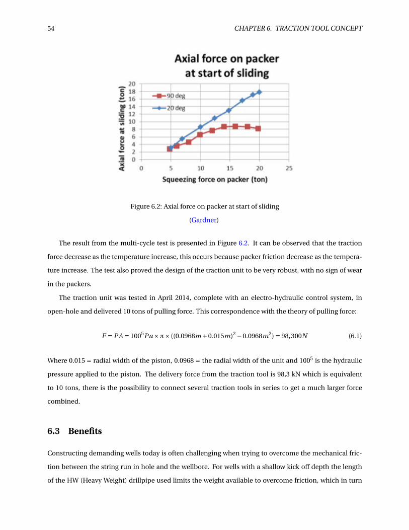
54 CHAPTER 6. TRACTION TOOL CONCEPT
Figure 6.2: Axial force on packer at start of sliding
(Gardner)
The result from the multi-cycle test is presented in Figure 6.2. It can be observed that the traction
force decrease as the temperature increase, this occurs because packer friction decrease as the tempera-
ture increase. The test also proved the design of the traction unit to be very robust, with no sign of wear
in the packers.
The traction unit was tested in April 2014, complete with an electro-hydraulic control system, in
open-hole and delivered 10 tons of pulling force. This correspondence with the theory of pulling force:
F = PA = 1005Pa ×π× ((0.0968m +0.015m)2 −0.0968m2) = 98,300N (6.1)
Where 0.015 = radial width of the piston, 0.0968 = the radial width of the unit and 1005 is the hydraulic
pressure applied to the piston. The delivery force from the traction tool is 98,3 kN which is equivalent
to 10 tons, there is the possibility to connect several traction tools in series to get a much larger force
combined.
6.3 Benefits
Constructing demanding wells today is often challenging when trying to overcome the mechanical fric-
tion between the string run in hole and the wellbore. For wells with a shallow kick off depth the length
of the HW (Heavy Weight) drillpipe used limits the weight available to overcome friction, which in turn

6.4. STATUS TODAY 55
minimize the completion length.
Rotation is avoided, in general, when running sand screens due to risk of mechanical damage and
limiting axial load capacity. Landing the string off depth, when zonal isolation packers are used, can
reduce productivity.
In light of the high daily rig rates today, improving operational efficiency by using a traction tool to
increase completion running speed can reflect in large cost savings. The risk for a completion string not
reaching its TD can result in an extra well section being drilled at a high additional cost in order to avoid
losing oil reserves. An outline description of the features of the traction tool includes:
• Capable of providing 10 ton pull on demand and up to 50 ton if put in series.
• Sturdy and simple control system.
• Fail safe.
• Completion fluid ensures hydraulic power.
• Low addition to total string weight.
• Compatible with other completion components.
6.4 Status Today
The traction tool has been a conceptual design for some time, it first started out as the HOP project back
in 2009 before the technology spin-off came a few years later. The goal is to take the traction device and
develop it into a full scale prototype to be qualified at the IRIS center (Ullrigg Drilling and Well Center).
The project is segregated into four main phases with decision gates:
1. Prototype Specification & Design — duration 8 months
2. Detailed Engineering — duration 6 months
3. Manufacturing, Assembly and Test — duration 10 months
4. Full-scale Qualification — duration 2 months
After each phase milestone reviews will be held with project partners and key project team members to
discuss the results and come to a consensus about moving to next phase.

56 CHAPTER 6. TRACTION TOOL CONCEPT
Figure 6.3: Overall project time line in a Gantt chart
6.4.1 Project Management
This phase is continuous throughout the project and involves reporting to relevant members, adminis-
tering contracts from partners and suppliers, follow-up on economics and overall risk management.
6.4.2 Prototype Specification & Design
Focusing on finalizing the design of the traction tool concept is the main task in this phase. There are four
main tasks to be executed; requirement specification, concept design,concept experiments and detailed
design.
The requirement specifications will be finalized with the involved partners through dialogue with
relevant experts and through a dedicated workshop event. Through the specifications all operational
requirements shall be considered alongside reviewing it for the relevant regulative framework.
Any design issues identified through the concept design work will be scrutinized through dedicated
experiments. One example will be to perform further traction packer testing to evaluate the effect of
different packer designs and materials under more demanding conditions.
At the end of this phase a detailed design of a primary traction unit will be finalized, comprising of all
components and interfaces. The phase is concluded with a design review meeting.

6.4. STATUS TODAY 57
6.4.3 Detailed Engineering
The target during this phase is to develop all the design documents mandatory for assembly, quality
control and operation of a HOP traction tool.
All aspects of the traction tool is investigated in detailed engineering; overall system, power delivery,
mechanical assemblies for traction, compatible with other completion components and the range of
operating conditions that may be met. The compatibility and the operating conditions will be attained
through technical meetings with the project partners.
Design details and material requirements will be examined using finite element analysis. Pertinent
document (quality control, assembly, test and operational procedures) is created.
Engineering will be performed in close participation with the primary suppliers and with design re-
views at suitable stop points.
This phase is concluded with an engineering review together with all partners and engineering sup-
pliers.
6.4.4 Manufacturing, Assembly and Test
The objective during this phase is to manufacture, assemble and bench test the traction tools. The plan
is to build two tools.
The main suppliers chosen during the detailed engineering work phase will be contracted for the
work required. The necessary parts and components will be machined and ordered.
There will be a close collaboration with the suppliers where they will be followed up during the fabri-
cation and all parts will be quality controlled. The traction tools will be built, tested and modified where
required. The fully assembled traction tool will undergo a function test on the bench and using other test
facilities.
All involved parties will be involved in a complete system review, where the detailed qualification test
program will be approved before initiating the final work phase.
6.4.5 Full-scale Qualification
The task is to develop test procedures including test site preparation, risk analysis and execution of the
test program.
The preparations for the test program will be done simultaneously along with the other phases and
will include:

58 CHAPTER 6. TRACTION TOOL CONCEPT
• Test objective description.
• Preparation of detailed test procedures, test analysis procedures, contingency plan and data re-
quirements
• Identifying and preparing the test site, planning for equipment transport, what recording equip-
ment and parameters to be used during the test, setting up the prototype
A back-up plan is included to allow for modifications to the traction tool and performing a second test
run. This allows to run a second test with alternate parameters, different modes of tool operation and/or
an industry demonstration.
A final project report will summarize the main project work, the test results and outline the plan for
the next phase.
6.5 Simulation
Before investing too much resources and time into this development project, a series of simulations were
run to confirm or contradict the theory behind the traction tool. The simulation software must correctly
calculate buckling, friction and have the possibility to add a positive force on the end of the string. Cer-
berus from NOV is the only simulation software commercially available that handles all these parameters.
Too make the simulations more realistic, data was gathered from the industry. An operator provided
data for one of its horizontal well, which had the highest amount of downtime while running a sand
screen completion. Well geometry, set casings, friction coefficients and fluid data was provided.
Simulations were performed with no axial force on end (traction tool not included in the simulation)
at first.

6.5. SIMULATION 59
Figure 6.5: Report from operator(sta)
Figure 6.4: Surface weight versus depth without traction tool
(NOV)
Looking at Figure 6.4 it is observed that the completion string goes into sinusoidal buckling at 3455
meter and helical buckling is observed at 4490 meter while RIH. As a result from this the screen will not
reach TD, the well will have a loss in production rate and loss in hydrocarbons recovery. Checking with
Figure 6.5, the report states that the string were not able to pass 4320 meter.
The simulation were run again, with the same parameters, with the exception of 35 tons that were
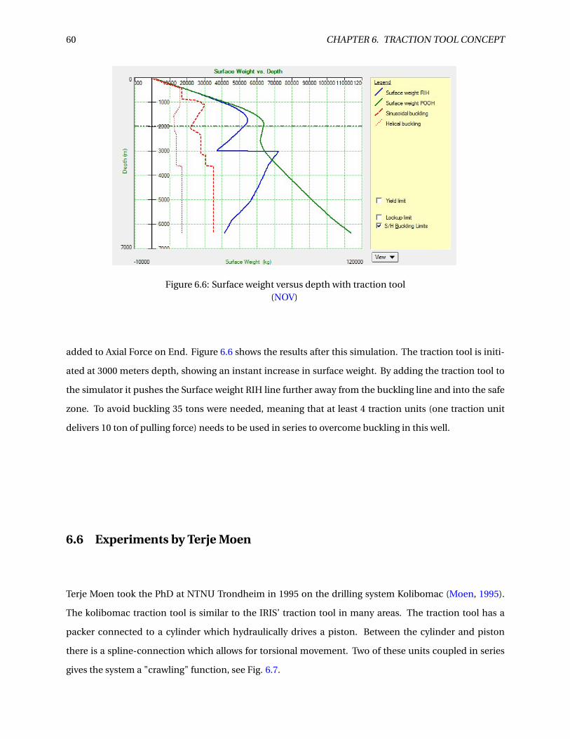
60 CHAPTER 6. TRACTION TOOL CONCEPT
Figure 6.6: Surface weight versus depth with traction tool(NOV)
added to Axial Force on End. Figure 6.6 shows the results after this simulation. The traction tool is initi-
ated at 3000 meters depth, showing an instant increase in surface weight. By adding the traction tool to
the simulator it pushes the Surface weight RIH line further away from the buckling line and into the safe
zone. To avoid buckling 35 tons were needed, meaning that at least 4 traction units (one traction unit
delivers 10 ton of pulling force) needs to be used in series to overcome buckling in this well.
6.6 Experiments by Terje Moen
Terje Moen took the PhD at NTNU Trondheim in 1995 on the drilling system Kolibomac (Moen, 1995).
The kolibomac traction tool is similar to the IRIS’ traction tool in many areas. The traction tool has a
packer connected to a cylinder which hydraulically drives a piston. Between the cylinder and piston
there is a spline-connection which allows for torsional movement. Two of these units coupled in series
gives the system a "crawling" function, see Fig. 6.7.

6.6. EXPERIMENTS BY TERJE MOEN 61
Figure 6.7: The traction tool has a hydraulic packer at each end. Packer A is inflated and cylinder A is
pressurized, pushing the piston forward (1 - 2). Cylinder B is simultaneously pushed forward, ready for
packer (B) inflation. (Moen, 1995)
The task for the packers is to centralize the traction tool and provide a seal, ensuring deflation of the
packers with over-pressure. Under normal operating conditions the packers will inflate towards the wall
and center the tool. Terje Moen ran a series of test on the packers to the Kolibomac traction tool with
regards to the expansion process and how the curvature holds up. The tool was run through a series of
test with different pressures and different length limitations. New packers needed to be found and tested
because of the standard packers used in the oil industry then were not meant to be continuously used.
The packer section were internally pressurized and the O.D. of the packers were written down. The
length limitations were ensured by installing steel rings in cavity A (Fig. 6.8)
Figure 6.8: Design of the packer section with relevant measurements
(Moen, 1995)
The summary of the tests conducted is summarized in Fig. 6.10. The curves with limited movement
show coinciding path for limited pressure and stiffer when compared to the unrestricted ends. When
the pressure exceeds 2 - 3 bar the slope decreases and is close to constant. The radius of curvature were
tested with the results in Fig. 6.9.

62 CHAPTER 6. TRACTION TOOL CONCEPT
Figure 6.9: Radius of curvature as a function of length along the packers under various pressures.
(Moen, 1995)
Figure 6.10: Increase in diameter as a function of pressure (free, 20mm, 5.8mm, locked down).
(Moen, 1995)
At low pressures there is a large gap in curvature radius between the middle of the packer and at the
end because of the stiffness of the rubber. When the pressure increases the curvature radii diminishes

6.6. EXPERIMENTS BY TERJE MOEN 63
and it evens out for the length of the packer.
6.6.1 Conclusion of the Kolibomac Project
A series of test were performed to map out the expansion path for reinforced packers. It was discovered
when the packer is expanded with no length limitations, only a small amount of pressure were needed
for a large expansion. At low pressures it is the stiffness in the rubber that will be dominant and thus the
packer will take the shape of a cylinder. Limiting the movement of the packer will change this drastically,
because the pressure will be absorbed by the reinforcement in the packer. The packers will then follow
the curvature of radii theory.
The theory behind curvature of radii was confirmed by calculating expansion measurements in a
packer. Knowing the coordinates for three points along the packer then using vector calculations will give
the radius of curvature. It was shown that the radius of curvature approaches a constant value through
the whole packer when pressure was increased, this shows the rubber stiffness will decrease over higher
pressures.
Chapter 7
Conclusion
Over the last decades the industry has seen dramatic changes in how operations are planned and exe-
cuted. Cost have increased, newly discovered fields prove to be a challenge developing and the focus on
high recovery has caused well completions to become more complicated.
Horizontal wells being planned are often cut short in length in fear that completion will not reach
TD. Because of the extreme length some of these wells can reach, there are a few issues to bear in mind
during the completion process. Particularly where buckling and lock-up are some of the most severe
issues encountered. One of these scenarios can have a large ripple-effect for the operation:
• unwanted downtime
• rig-rate and operational costs keep running during downtime
• possible loss of equipment
• loss of well in worst case
The industry has met some of these challenges with new technology (Chapter 1). However, the risk
regarding buckling and lock-up, has many operators working to avoid long horizontal wells (e.g. drilling
multiple subsea wells and tying them back to existing structures).
Implementing the traction tool concept from IRIS can aid the operator to successfully completing
long horizontal wells more effectively. The simulations performed in chapter 6 indicate that this is achiev-
able. The traction tool will provide a drag force, which in effect will keep the drillstring in constant ten-
sion.
One of the Norwegian Petroleum Directorate’s tasks is to ensure that the recovery rate increases in
the future. This will affect what types of wells will be drilled and completed. Completion technologies are
64

65
equipped to handle today’s challenges, but companies need to develop appropriate technology to meet
tomorrow’s challenges. The traction tool concept is a step in the right direction.

66

67
Chapter 8
Acronyms
WWS — Wire Wrapped Screen
PPS — Pre-Packed Screen
PSD — Particle Size Distribution
LPSA — Laser Particle Size Analysis
ASTM E11-13 — Standard Specification for Woven Wire Test Sieve Cloth and Test Sieves
SL — Slotted Liner
MMS — Metal-Mesh Screen
OHGP — OpenHole Gravel Pack
T&D — Torque and Drag
UCS — Unconfined Compressive Strength
NTG — Net To Gross
PVT — Pressure, Volume, Temperature
ICD — Inflow Control Device
FEA — Finite Element Analysis
λ — Helix Angle
DLS — DogLeg Severity
µ — Friction Factor
NOV — National Oilwell Varco
CTES — Coiled Tubing Engineering Service
TFM — Tubing Forces Model
RIH — Run Into Hole
NCS — Norwegian Continental Shelf
SAGD — Steam Assist Gravity Drainage
IRIS — International Research Institute of Stavanger
ECP — External Casing Packer
HOP — Hole in One Producer
TD — Target Depth
O.D. — Outer Diameter
I.D. — Inner Diameter
CT — Coiled Tubing
WL — WireLine
CBL — Cement Bond Log

Bibliography
http://www.geomore.com/rock-cores/.
http://www.bakerhughes.com/products-and-services/evaluation/coring-services/
wireline-sidewall-coring-services.
http://www.scientificamerican.com/slideshow/how-to-turn-tar-sands-into-oil-slideshow/.
http://www.haverbrasil.com.br/telas/en/haver_eml_200_digital_plus.php/.
http://www.sand-screen.com/product/wire-wrapped-screen.html.
http://particle.dk/methods-analytical-laboratory/particle-size-by-laser-diffraction/
laser-diffraction-theory/.
http://www.welltec.com/solutions/conveyance/.
E-mail correspondence with statoil.
Lotorq, mechanical friction- and wear-reduction centralizer system.
Aadnøy, B. S. (2010). Modern Well Design. CRC Press.
Aasen, J. A. and Aadnøy, B. S. (2002). Buckling models revisited. SPE 77245.
Bellarby, J. (2009). Well Completion Design, volume 56 of Developments in Petroleum Science. Elsevier,
Amsterdam, The Netherlands, 1st edition.
Bhalla, K. et al. (1994). Implementing residual bend in a tubing forces model. SPE paper, 28303:69.
Chen, Y.-C. (1988). Post buckling behavior of a circular rod constrained within an inclined hole. PhD
thesis, Masters Thesis, Rice University. http://hdl. handle. net/1911/13278.
68

BIBLIOGRAPHY 69
Dawson, R. and Paslay, P. R. (1984). Drillpipe buckling in inclined holes. J. Petrol. Tech., SPE 11167, pages
1734–1738.
ExxonMobil, L. P. (2011). Tta3: Future technologies for cost-effective drilling and intervention. OG21.
Gardner, D. Evaluation of hop liner and sand screen traction applications. IRIS Internal.
Ian C. Walton, S. (2001). Perforating unconsolidated sand: An experimental and theoretical investigation.
SPE 71458.
J. C., C. (2003). Buckling of tubulars inside wellbores: A review on recent theoretical and experimental
works. SPE 80944.
Ken Newman, Kenneth Bhalla, A. M. Basic tubing forces model (tfm) calculation.
Lubinski, A. A. (1962). Helical buckling of tubing sealed in packers. SPE 178.
March Haci, J. H. (2001). New coiled tubing well tractor extends lateral reach. SPE.
Mitchell, F. R. and Miska, S. (2004). Helical buckling of pipe with connectors and torque. SPE 87205.
Mithell, R. F. (2001). Lateral buckling of pipe with connectors in curved wellbores. SPE 67727.
Moen, T. (1995). Utvikling og testing av foringsmodul for utstøpning av et konsentrisk rør i et borehull for
systemet Kolibomac. PhD thesis, NTNU.
M.S. Aston, P. H. and McGhee, G. (1998). Techniques for solving torque and drag problems in today’s
drilling environment. SPE 48939.
NOV, C. Ctes product catalogue.
R. F., M. (1996). Buckling analysis in deviated wells: A practical method. SPE 36761.
Rimereit, B. E. (2015). Meetings.
Standard, A. N. (2013). Standard Specification for Woven Wire Test Sieve Cloth and Test Sieves.
Weatherford (2015a). Sand screen selector.
Weatherford (2015b). Well screen technologies.
X., H. and A., K. (1995). Helical buckling and lock-up conditions for coiled tubing in curved wells. SPE
25370.