master’s thesis an adaptive routing protocol with ... · anthocnet has higher delivery...
TRANSCRIPT

Master’s Thesis
Title
An Adaptive Routing Protocol with Attractor Selection
for Mobile Ad Hoc Networks
Supervisor
Professor Masayuki Murata
Author
Narun Asvarujanon
February 15th, 2010
Department of Information Networking
Graduate School of Information Science and Technology
Osaka University

Master’s Thesis
An Adaptive Routing Protocol with Attractor Selection for Mobile Ad Hoc Networks
Narun Asvarujanon
Abstract
Mobile Ad Hoc Networks (MANETs) have various advantages over a traditional wired net-
works, e.g., requiring no fixed infrastructure and allowing arbitrary movement and participation
of mobile nodes. However, routing in MANETs faces many difficulties, e.g., frequent topology
changes and a multiple access medium which is easily interfered by other radio signals. Many
MANET routing protocols have been proposed to handle these problems in the past. Unfor-
tunately, they require a considerable amount of undesirable overhead especially in the unstable
conditions like failures and mobility. Therefore, we aim at designing a MANET routing protocol
which is adaptive against topology changes and packet collisions while having low overhead.
In this thesis, we propose a biologically-inspired routing protocol for MANETs. As biologi-
cal systems are well-known for their self-adaptability against a changing environment, we adopt
the biologically-inspired mechanism, calledattractor selection, in the next hop selection process
for routing in MANETs. Our protocol is a noise-driven and feedback-based on-demand routing
protocol which is based on the previously proposedmobile ad hoc routing with attractor selection
(MARAS). Unlike the original protocol, which uses a simplified packet level routing, we extend
MARAS to fully operate within the IEEE 802.11 protocol stack without such limitations.
The main contribution of this thesis lies in the route maintenance mechanism performed by
using a feedback packet for each delivered data packet. In respect to this mechanism, the route
recovery can be achieved without using additional broadcast control packets like most of the on-
demand routing protocols, e.g. AODV. Comparing to AODV, MARAS can achieve up to 48%
higher delivery efficiency while having approximately 42% lower overhead in the failure scenarios.
In mobility scenarios, MARAS and AODV have roughly the same performance. MARAS is also
compared to another biologically-inspired protocol, AntHocNet, and is found to have much lower
overhead. AntHocNet has higher delivery efficiency than MARAS only in the scenarios with low
traffic and dynamics, but it is inferior to MARAS in the most cases of the evaluation.
1

Keywords
Ad hoc networks
Routing protocol
Biologically-inspired networking
Attractor selection mechanism
2

Contents
1 Introduction 8
2 Related Work 12
2.1 Conventional Routing Protocols . . . . . . . . . . . . . . . . . . . . . . . . . . 12
2.1.1 Proactive Routing Protocols . . . . . . . . . . . . . . . . . . . . . . . . 12
2.1.2 Reactive Routing Protocols . . . . . . . . . . . . . . . . . . . . . . . . . 14
2.1.3 Hybrid Routing Protocols . . . . . . . . . . . . . . . . . . . . . . . . . 17
2.2 Biologically-inspired Routing Protocols . . . . . . . . . . . . . . . . . . . . . . 18
3 Attractor Selection-based Mathematical Model 21
3.1 Attractor Selection Mechanism . . . . . . . . . . . . . . . . . . . . . . . . . . . 21
3.2 Mathematical Model for MANET Routing Protocol . . . . . . . . . . . . . . . . 23
4 Mobile Ad Hoc Routing with Attractor Selection (MARAS) 25
4.1 Route Establishment . . . . . . . . . . . . . . . . . . . . . . . . . . . . . . . . 25
4.2 Routing Information . . . . . . . . . . . . . . . . . . . . . . . . . . . . . . . . 27
4.3 Data Packet Forwarding . . . . . . . . . . . . . . . . . . . . . . . . . . . . . . . 28
4.4 Route Maintenance . . . . . . . . . . . . . . . . . . . . . . . . . . . . . . . . . 29
4.4.1 Feedback Packet . . . . . . . . . . . . . . . . . . . . . . . . . . . . . . 29
4.4.2 Activity Calculation . . . . . . . . . . . . . . . . . . . . . . . . . . . . 30
4.4.3 Activity Decay and Routing Vector Update . . . . . . . . . . . . . . . . 30
4.4.4 Attractor Selection-based Route Recovery . . . . . . . . . . . . . . . . . 31
4.4.5 Local Connectivity Maintenance . . . . . . . . . . . . . . . . . . . . . . 33
5 Evaluation 34
5.1 Simulation Configurations . . . . . . . . . . . . . . . . . . . . . . . . . . . . . 35
5.1.1 Terrain Size and Node Placement . . . . . . . . . . . . . . . . . . . . . 35
5.1.2 Wireless Configuration and Traffic . . . . . . . . . . . . . . . . . . . . . 36
5.1.3 Protocol Parameters . . . . . . . . . . . . . . . . . . . . . . . . . . . . 37
5.1.4 Failure Model . . . . . . . . . . . . . . . . . . . . . . . . . . . . . . . . 38
5.1.5 Mobility Model . . . . . . . . . . . . . . . . . . . . . . . . . . . . . . . 39
3

5.2 Failure Scenario . . . . . . . . . . . . . . . . . . . . . . . . . . . . . . . . . . . 39
5.2.1 Single Session Failure Scenario . . . . . . . . . . . . . . . . . . . . . . 39
5.2.2 Multiple Sessions Failure Scenario . . . . . . . . . . . . . . . . . . . . . 42
5.3 Mobility Scenario . . . . . . . . . . . . . . . . . . . . . . . . . . . . . . . . . . 44
5.3.1 Single Session Mobility Scenario . . . . . . . . . . . . . . . . . . . . . 44
5.3.2 Multiple Sessions Mobility Scenario . . . . . . . . . . . . . . . . . . . . 45
5.4 Discussion on Random Walk Range (ρ) Parameter in MARAS . . . . . . . . . . 47
5.5 Discussion on Adaptability . . . . . . . . . . . . . . . . . . . . . . . . . . . . . 48
6 Conclusion and Future Work 50
Acknowledgments 51
References 56
4
List of Figures
1 Communication in mobile ad hoc networks . . . . . . . . . . . . . . . . . . . . 8
2 Behavior of attractor selection system . . . . . . . . . . . . . . . . . . . . . . . 22
3 Dynamics ofM alternatives’ values from attractor selection model (M = 6) . . . 24
4 Overview of MARAS . . . . . . . . . . . . . . . . . . . . . . . . . . . . . . . . 26
5 Example of the next hop selection using state values . . . . . . . . . . . . . . . . 29
6 Maximum value switching whenα < θ . . . . . . . . . . . . . . . . . . . . . . 32
7 Example of failure scenario . . . . . . . . . . . . . . . . . . . . . . . . . . . . . 36
8 Example of mobility scenario . . . . . . . . . . . . . . . . . . . . . . . . . . . . 37
9 Evaluation results against number of failure occurrences (1 session, 256 nodes) . 40
10 Evaluation results against number of nodes (1 session, 256 nodes) . . . . . . . . 42
11 Evaluation results against number of failure occurrences (2 sessions, 256 nodes) . 43
12 Evaluation results against number of nodes (2 sessions, 256 nodes) . . . . . . . . 44
13 Evaluation results against maximum speed (1 session, 256 nodes) . . . . . . . . 45
14 Evaluation results against maximum speed (10 sessions, 256 nodes) . . . . . . . 46
15 Effects of random walk rangeρ in mobility scenarios (maximum speed = 10 m/s) 47
5

List of Tables
1 Summary of MANET routing protocols . . . . . . . . . . . . . . . . . . . . . . 12
2 Summary of simulation configurations . . . . . . . . . . . . . . . . . . . . . . . 35
3 Simulation parameters of MARAS . . . . . . . . . . . . . . . . . . . . . . . . . 38
6

1 Introduction
Mobile Ad Hoc Networks (MANETs) have been receiving a lot of research attention in the last
few decades. MANETs differ from the traditional wired networks because they are independent
of a fixed infrastructure; this allows the mobile nodes to move freely and makes many useful
applications possible, e.g., rescue mission in an infrastructure-less area. However, this flexibility
causes difficulties in routing. Examples of these difficulties are [1]:
1) Unpredictable dynamic changes in topology which is caused by the arbitrary movement and
participation of the member nodes as shown in Figure 1.
2) Decentralized control as each node has to maintain the route locally with only partial network
information.
3) Limited bandwidth as the wireless channel uses a multiple access method, e.g., CSMA/CA,
and each transmission interferes with each other.
4) Limited energy of the mobile node.
Figure 1: Communication in mobile ad hoc networks
7

Due to these difficulties, a routing protocol should not create high control overhead due to limited
bandwidth and energy despite the need of control mechanisms for handling the network dynamics.
Designing such routing protocols is a challenging task; therefore, one of the most active research
activities on MANETs is on routing protocols.
Many MANET routing protocols have been proposed in the past and they can be distinguished
into three main categories:proactive, reactive, andhybrid protocols. The proactive protocols ex-
change control messages between nodes periodically to maintain a consistent view of the network
even when there is no active data session. This allows the proactive protocol to discover the route
quickly at the price of large bandwidth consumption from the overhead in exchanging control
message. Moreover, there is a waste of network resources because every node has to maintain the
complete view of the network even though most routing information is never used. In contrast,
the reactive protocols establish and maintain the route between the source and the destination only
if there is a request. Because of this characteristic, these protocols are also calledon-demand
protocols. The established route is maintained as long as the data session is active. After a cer-
tain period of time, when the data session becomes inactive, the route is removed to release the
occupied resources. Therefore, reactive protocols consume less bandwidth than proactive proto-
cols. However, due to the dynamic characteristic of the ad hoc network, the packet might suffer a
variable and long delay as the route discovery/recovery might have to be performed at each hop it
travels through. To overcome these weaknesses of both proactive and reactive protocols, the hy-
brid protocols have been proposed. In hybrid protocols, groups of nodes—often calledzones, are
formed and a proactive routing method is used within each zone while a reactive routing method
is used to communicate with remote nodes. Most hybrid protocols separate nodes into flat zones
and a few use hierarchical structures like trees or clusters [2]. With this method, the overhead is
reduced because the inefficient control overhead of the proactive approach is limited only within
the zone and and the lower overhead from reactive routing is used to efficiently connect each zone.
However, the performance of hybrid protocols often relies on the trade-off in parameters like the
zone radius, which needs to be particularly adjusted to each network before use.
Examples of well-known proactive protocols are the destination-sequenced distance vector
(DSDV), which offers a loop-free route by using the distance vector shortest path routing algo-
rithm [3], and the optimized link state routing (OLSR), which attempts to reduce the flooding
overhead by using optimized (partial) link state information [4]. Among the on-demand proto-
8

cols, the well-known protocols are the dynamic source routing protocol (DSR) and the ad hoc
on-demand distance vector routing (AODV). DSR requires low overhead as it does not require any
periodic control messages and it can lower the route discovery overhead using a caching mech-
anism [5]. AODV uses a routing table at each node to achieve quick route recovery in dynamic
conditions [6]. Examples of well-known hybrid protocols are the zone routing protocol (ZRP) [7]
and the zone-based hierarchical link state (ZHLS) [8]. More details of existing MANET routing
protocols and their features are discussed in Section 2.
We focus our research on on-demand protocols because they require less overhead than proac-
tive protocols in order to adapt to changes in the network and proactive methods consume too
much energy in exchanging the routing information on a periodic basis, especially pure proac-
tive protocols like DSDV. In addition, it has been shown that DSR is better than OLSR in terms
of energy consumption [9]. Among the on-demand protocols, AODV is more scalable and more
adaptive than DSR as shown in [10]. However, AODV has its own weaknesses, i.e., it causes
high load on the network because of routing overhead (mainly flooding) and it does not take the
link qualities into account, which possibly results in selecting unstable links [11]. Therefore, we
aim at designing a new routing protocol, which is more adaptive against unstable conditions in
the network and causes lower overhead than AODV. Optimizing this newly proposed protocol by
converting it into a hybrid protocol can be considered as a future work.
To achieve robustness and adaptability, we consider a biologically-inspired mechanism. As
biological systems are well-known for their robustness and adaptability, there is a lot of research
adopting mechanisms inspired by biology, e.g., swarm intelligence [12], which is a very active
field of research, and ant colony optimization (ACO) [13], which is also based on swarm intel-
ligence and useful for solving optimization problems. For MANETs, many biologically-inspired
routing protocols have been proposed and most of them are based on swarm intelligence, e.g.,
AntHocNet [14], BeeAdHoc [15], and HOPNET [16]. Note that our protocol however uses a
biologically-inspired mechanism from cell biology calledattractor selectionand is not based on
swarm intelligence. The reason is that the concept of routing with the attractor selection mech-
anism has been found simple yet robust to failures [17, 18]. Moreover, our purpose is also to
discover a new alternative of biologically-inspired mechanisms other than social insects-based
swarm intelligence for MANETs.
9

Our adaptive mobile ad hoc routing with attractor selection (MARAS) is an extended work
from [17, 18]. Unlike the original protocol, which focused only on the basic routing mechanism
using simplified assumptions on packet level, we remove such limitations and evaluate MARAS
with the QualNet network simulator [19], which fully operates in the IEEE 802.11 protocol stack.
MARAS is a noise-driven on-demand protocol which uses feedback of delivered data packets
from the destination for route maintenance. Using the feedback information along with the at-
tractor selection mechanism allows MARAS to recover from link failures without issuing any
additional broadcast control message like AODV. According to the evaluation results, in most
scenarios MARAS has higher delivery efficiency than AODV and in failure scenarios with high
node density it also achieves lower transmission overhead. MARAS has only slightly lower de-
livery efficiency and higher overhead per successfully delivered packet than AODV in mobility
scenarios. We also compare MARAS to another biologically-inspired protocol—AntHocNet. The
results show that MARAS has lower delivery efficiency than AntHocNet only in scenarios with
low failure occurrences, low traffic load, or low node density. However, MARAS generally has
much lower overhead than AntHocNet and it completely outperforms AntHocNet in the rest of
considered scenarios of the evaluation.
The rest of this thesis is organized as follows. First, we present some of the most important
routing protocols for MANETs in the next section. Then, we introduce the attractor selection
mechanism and the derived mathematical model in Section 3. Afterward, we describe our protocol
in Section 4. In Section 5, the evaluation results are presented and discussed. Finally, we conclude
and list future work in Section 6.
10
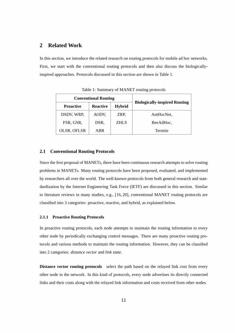
2 Related Work
In this section, we introduce the related research on routing protocols for mobile ad hoc networks.
First, we start with the conventional routing protocols and then also discuss the biologically-
inspired approaches. Protocols discussed in this section are shown in Table 1.
Table 1: Summary of MANET routing protocols
Conventional RoutingBiologically-inspired Routing
Proactive Reactive Hybrid
DSDV, WRP, AODV, ZRP, AntHocNet,
FSR, GSR, DSR, ZHLS BeeAdHoc,
OLSR, OFLSR ABR Termite
2.1 Conventional Routing Protocols
Since the first proposal of MANETs, there have been continuous research attempts to solve routing
problems in MANETs. Many routing protocols have been proposed, evaluated, and implemented
by researchers all over the world. The well-known protocols from both general research and stan-
dardization by the Internet Engineering Task Force (IETF) are discussed in this section. Similar
to literature reviews in many studies, e.g., [16, 20], conventional MANET routing protocols are
classified into 3 categories: proactive, reactive, and hybrid, as explained below.
2.1.1 Proactive Routing Protocols
In proactive routing protocols, each node attempts to maintain the routing information to every
other node by periodically exchanging control messages. There are many proactive routing pro-
tocols and various methods to maintain the routing information. However, they can be classified
into 2 categories:distance vectorandlink state.
Distance vector routing protocols select the path based on the relayed link cost from every
other node in the network. In this kind of protocols, every node advertises its directly connected
links and their costs along with the relayed link information and costs received from other nodes.
11

One example of distance vector routing protocols is thedestination-sequenced distance-vector
protocol (DSDV) [3], which uses the number of hops to the destination as the cost. The routing
information is advertised in a broadcast manner throughout the network along with the sequence
number, which is originally generated by the destination. The sequence number is used to avoid a
routing loop problem which is a common problem in distance vector routing. DSDV reacts to the
topology changes using two kinds of update packets:full dumpand incremental. The full dump
packets will carry all available routing information at the current node to another while the incre-
mental packets will carry only the information changed since the last full dump. These two types
of routing update packets are used to lower the overhead and shorten the update latency. However,
the overhead of DSDV is still large due to the large amount of periodic update information, which
makes DSDV not scalable [2].
Another example is thewireless routing protocol(WRP) [21]. In WRP, each node maintains
four tables: a distance table, a routing table, a link-cost table, and a message retransmission list.
WRP uses the predecessor information along with the sequence number to avoid routing loops.
In addition to the bandwidth consumption overhead, WRP also has a high memory consumption
overhead due to the large amount of information maintained at each node.
Link state routing protocols maintain a complete view of the network and construct a routing
tree for data packet forwarding. To obtain a complete network view, a large amount of routing
information is exchanged among nodes. Similar to distance vector protocols, link state protocols
also have a high overhead where a large amount of bandwidth is consumed by routing control
packets.
One example of link state routing protocols is thefisheye state routing(FSR) [22, 23]. FSR
maintains a topology map at each node by exchanging the link state information between neigh-
bor nodes. However, the link state packets are not broadcasted and only periodically exchanged
with the local neighbor nodes. FSR reduces the amount of control overhead by removing the
event-based link state update and using only the periodic update. Moreover, the periodic update
frequency is reduced by the fisheye technique where the node within the smaller scopes updates
more frequently than the node that is farther away. FSR is based on the global state routing
(GSR) [24], which can be viewed as a special case of FSR where the scope is∞. The advantages
of FSR are that the flooding is minimized and the routing is more accurate for nodes closer to the
12

destination, which makes it suitable for dense networks. However, the slower update for remote
nodes affects the accuracy and by using this imperfect topology information an inaccurate route
selection could possibly occur.
Another example is theoptimized link state routing(OLSR) [4]. In OLSR, each node periodi-
cally floods a list of its 1-hop neighbors. However, instead of relaying all link information, OLSR
diffuses only the partial link information through the multipoint relays (MPRs) which cover all
2-hop neighbor nodes. Therefore, the complete topology can be obtained while the amount of
link state information is reduced. However, flooding the 1-hop neighbor list at each node is still
not suitable in MANET and causes high overhead in large networks. Regarding this, there is a
proposal of the FSR-OLSR combination which is called OFLSR (or F-OLSR) [25] in the field of
wireless mesh networks. According to the evaluation in [26, 27], OFLSR offers higher delivery
ratio and lower delay than AODV which is a reactive routing protocol. However, the overhead of
OFLSR is still much higher than AODV.
In summary, most of the proactive routing protocols are not well scalable due to the amount
of routing control overhead. The delivery efficiency and delay are generally better than reactive
routing protocols by exploiting this extra amount of overhead. Many attempts have been made to
reduce the overhead and one of the considerably successful methods is hierarchical routing like
OLSR. However, the selection of representative nodes, like MPR in OLSR or cluster heads in other
hierarchical routing is also a disadvantage of this kind of routing protocols in a mobility scenario.
As a result, it may require more overhead in MANET where mobility is one of its characteristics.
Additionally, maintaining all the link information can be considered unnecessary because most of
the links are not used. Regarding this matter, reactive routing protocols can be considered more
suitable in MANETs.
2.1.2 Reactive Routing Protocols
Reactive routing protocols, also known as on-demand routing protocols, have been proposed to
reduce the number of control overhead by maintaining only the information for active routes.
Instead of maintaining all the routes at all times, the protocol starts route discovery on-demand. In
the route discovery process, a route request packet (RREQ) is usually flooded until it reaches the
destination (or a node that contains the route to the destination). Then, a route reply packet (RREP)
is generated and sent back to the source to inform the available route. This route is maintained as
13

long as the connection is active and removed once it is no longer required. In general, on-demand
routing protocols can be classified into 2 categories:hop-by-hop routingandsource routing.
Hop-by-hop routing protocols maintain the routing information locally at each node. The data
packet stores only the destination address in its header and each intermediate node will use its
routing table to forward the packet to the specified destination. The advantage of this approach is
the high adaptability of the path because each node can react to the changes in the network faster
than the end-to-end manner. However, maintaining the routing information at each node requires
higher routing overhead and resources.
An example of hop-by-hop routing protocols is thead hoc on-demand distance vector routing
(AODV) [6]. The standard AODV uses the broadcast route request packet to discover the route to
the destination. Once the route request arrives at the destination, the route reply packet is sent back
to the source using the reverse route previously established by the route request packet. AODV
uses a blacklist to avoid using unidirectional links, which are the links established by the route
request packet but cannot be utilized by the route reply packet. Moreover, the precursor list is
maintained to keep track of the upstream node that is utilizing this route. When a route failure
occurs, a route error packet is sent out in broadcast manner if the precursor list is not empty.
This route error packet is repeatedly flooded until it reaches the source node or the node with an
empty precursor list. Once the source node receives the route error packet, the route recovery
which is the same process as the route establishment using route request and route reply packets
is repeated. Regarding the route recovery process, the local route repair feature of AODV can be
chosen. Instead of re-initiating the route discovery from the source, the delay can be reduced by
initiating it from the node that detects the error. Also, another feature of AODV which allows the
intermediate nodes to respond to the RREQ can be chosen to further shorten the delay.
Source routing protocols maintain the routing information only at the source. A list of ad-
dresses that the packet will traverse until it reaches the destination is embedded into the header of
each packet by the source. Each intermediate node has no knowledge of the route to destination
and only forwards each data packet by the information in its header. As maintaining the route at
each intermediate node is no longer required, the overhead is reduced. However, the probability
of route failures could be high when the path becomes long in large networks or when there is a
14
high level of mobility. Moreover, the overhead of embedded route information in the header also
affects the performance in large networks. According to these disadvantages, it can be clearly seen
that source routing protocols do not scale well.
An example of source routing protocols is thedynamic source routing(DSR) [5]. DSR is a
simple source routing protocol composed of two mechanisms: route discovery and route mainte-
nance. Both mechanisms operate purely reactive, which means that if there is not any change in
the network, then there will be no additional control packet. DSR supports multiple routes which
help decrease the delay upon the failure of the currently used route. Other than source-initiated
flooding route discovery, each node allows to cache the overheard embedded route information
in each data packet which increases the number and freshness of possible routes. When any link
on a route is broken, a route error packet (RRER) is sent back to inform the source. Upon the
RRER arrival, the broken route is removed and another available route will be selected or the
route discovery process will be re-initiated. According to this behavior, DSR should have a very
low routing overhead. It has been shown in [10] that DSR performs better than AODV in terms of
delay and overhead in a less “stressful” scenarios, e.g., low number of sources, low mobility, etc.
However, AODV performs better than DSR in terms of delay but still has higher routing overhead
in a more stressful scenario, which is more likely to occur in real world applications.
Another source routing protocols is theassociativity-based routing for ad-hoc mobile net-
works (ABR) [28]. ABR is a special case of source routing protocols because it uses a similar
route discovery to DSR but also maintain local route information like AODV. Rather than hav-
ing multiple backup routes like DSR, ABR focuses on the stability of the route. ABR selects the
route based on a metric, called associativity tick, which reflects the degree of association stabil-
ity of mobile nodes. The associativity ticks are maintained by periodic beacons from each node.
During the route discovery, not only the addresses are embedded in the packet’s header but also
the associativity tick is included to allow an intermediate node and the destination to select the
best path according to all associativity ticks of upstream nodes. As ABR does not have backup
routes, a route reconstruction is required upon link failures. Even though this route reconstruction
is performed locally, it can still cause a longer delay and more control overhead.
In summary, reactive routing protocols generally require less overhead than proactive routing
protocols as they maintain only necessary routing information. In [9], it was shown that DSR
achieves lower overhead, higher throughput, and longer node lifetime than OLSR over variable
15

mobility and connection patterns. On the other hand, the only strong point of OLSR is the shorter
delay as it is the common advantage of proactive routing protocols. According to this research,
it can be seen that in general reactive routing protocols are more suitable than proactive routing
protocols except where the application requires very short delays. When comparing among differ-
ent reactive protocols, AODV is more adaptive than DSR as it can maintain higher throughput and
shorter delays in the network scenarios with higher dynamics [10]. As we focus on the adaptability
of the routing protocol, we use AODV as the reference protocol in this thesis.
2.1.3 Hybrid Routing Protocols
Hybrid routing protocols use the combination of proactive routing and reactive routing concepts
for the purpose of increasing scalability. In hybrid protocols, the network is partitioned into zones.
A proactive routing method is used within each zone while a reactive routing method is used to
communicate with nodes that are outside of the zone. With this method, the overhead is reduced
because the inefficient control overhead of the proactive approach is limited only within the zone
and the lower overhead from reactive routing is used to efficiently connect each zone. In this
section, we show four examples of hybrid routing protocols as follows.
The first example is thezone routing protocol(ZRP) [7]. ZRP reduces the proactive routing
overhead by limiting the scope of proactively maintaining the routing information within a zone.
A zone is defined by the hop distance between nodes where the nodes withinρ hops from the
current node are in the same zone. ZRP discovers the path to the node outside the zone using
bordercasting, which also reduces the number of flooding messages. In bordercasting, the route
request packet is forwarded only by the border node of the current zone. When the route request
packet is received, the border node looks up the proactive routing table in its zone and sends back
the route reply packet if it has the route to the destination or repeats the bordercasting process
otherwise. The routing zone radiusρ is a very crucial parameter in ZRP which also becomes a
disadvantage of ZRP. The radiusρ must be carefully chosen based on the characteristic of the
network. If the radius is too large, then ZRP behaves more like a pure proactive protocol. On the
other hand, if the radius is too small, then ZRP behaves more like a pure reactive protocol. In both
cases, ZRP loses its advantage of reduced overhead and scalability.
The second example is thezone-based hierarchical link state(ZHLS) [8]. ZHLS is a zone-
based hierarchical link state routing protocol, which also uses the location information from the
16

global positioning system (GPS). In contrast to ZRP which defines overlapping zones, ZHLR
utilizes the location information to partition the network into non-overlapping zones and assign
each node a node ID and a zone ID. The hierarchical topology consists of two levels: a node
level and a zone level. There is no cluster-head in ZHLS because the zones are pre-designed
with regard to their location information. Hence, a single point of failure or bottlenecks can be
avoided in ZHLS despite being a hierarchical routing protocol. The routing mechanism consists of
intrazone proactive routing and interzone reactive routing which is similar to ZRP. Therefore, the
similar advantages can be achieved. Additional advantages of ZHLS are the fixed zone location.
Once the source node knows the node ID and the zone ID of the destination, even if the link
breaks, ZHLS can still easily find another route to the destination with less overhead compared to
reactive routing protocols. However, this fixed zone location is also the disadvantage of ZHLS as
it is required to be preprogrammed before use.
In summary, hybrid routing protocols use the integration between proactive and reactive pro-
tocols to increase the scalability. Lower delay and overhead can be expected from this kind of
protocols even in large scale networks. However, our research objective is to design an adaptive
routing protocol. It should be able to adapt to any network without any adjustment. On the other
hand, hybrid routing protocols require proper tuning of parameters, like routing zone radius in
ZRP or preprogrammed zone maps in ZHLS for each network. Therefore, we do not rely on the
hybrid routing approaches in our protocol.
2.2 Biologically-inspired Routing Protocols
As stated above, the traditional routing protocols face a lot of problems due to the dynamic be-
havior and resource constraints in MANETs. To overcome this limitation, a routing protocol is
required to have a self-organizing or an autonomous feature. An approach to achieve such feature
is to use a biologically-inspired mechanism.
Once we look into the nature, a living organism, or a biological system, it can be seen that
they can maintain their stable condition by themselves regardless of the external influences or
dynamic conditions. For example, the human immune system can fight against the external threats,
like virus or bacterias, to recover the body to normal state without any explicit control from the
brain. In biological systems, each small entity works separately to lead the entire system to an
equilibrium condition. One of the biological systems that have received a lot of research attention
17

is swarm intelligence [12].
The concept of swarm intelligence originates from the social behavior of insect colonies, such
as ant colonies. We explain some swarm intelligence-based routing protocols in this section. First,
the ant-based routing protocols are discussed. Afterward, we describe the other social insect-based
routing protocols.
The main algorithm of ant-based routing protocol is the Ant Colony Optimization (ACO) [13].
ACO is based on the foraging process of ants which is a random walk when searching for food.
Once the food is found, the ant returns to the nest via its own trail. While returning, the ant
deposits pheromones on the way as chemical markers for other ants to follow its trail to the food.
The indirect communication, which is based on the pheromone trail mediated by the environment,
is calledstigmergy. Using this approach, the shortest path between the source and the destination
can be found.
The first ant-based routing protocol, called AntNet [29], is designed for a wired network.
AntNet uses two kinds of agents, forward and backward ants, to find the shortest path. The forward
ant moves toward the destinationd via a neighbor noden according to a greedy stochastic policy
based on the ant’s visited node list, the pheromone informationPnd, and the heuristic functionln
based on the queue length of the link connecting to neighborn. To avoid congestion, the forward
ant is released based on the probability valuepd which changes according to the current traffic
load. At the destination, the forward ants turn into the backward ants and return to the source
on the same path the forward ants had taken. While returning, the pheromone information and
other statistical information gathered by forward ants are used to update the routing table of each
intermediate node.
The early attempt of applying ACO on MANET routing is theant-colony based routing al-
gorithm for MANETs(ARA) [30]. Even though ARA is based on the same ACO as AntNet, it
is a reactive routing protocol consisting of three phases: route discovery, route maintenance, and
route failure handling. ARA sets up the path reactively using the forward ant (FANT) and the
backward ant (BANT) in the route discovery process. Different from the original ACO, the agent
in ARA does not memorize the visited nodes. Instead, each intermediate node uses the source and
the previous hop of the FANT and creates the route entry accordingly. Routing loops are avoided
by using a sequence number like in other reactive protocols. The route maintenance is performed
using the reinforcement by data packets. The failure handling re-initiates a route discovery when
18

there is no alternative link in the routing table.
Another well-known ant-based routing protocol is theant-based hybrid routing algorithm for
mobile ad hoc networks(AntHocNet) [14], which uses both pheromone and visited node list sim-
ilarly to AntNet. In AntHocNet, the route is set up reactively usingreactive forward antswhich
gather the path quality while travelling in the network. Upon arrival at the destination,backward
antsreturn on the path taken by forward ants to the source and update the routing tables of nodes
on the path. Unlike ARA, AntHocNet usesproactive forward antsto maintain the paths. These
ants follow the pheromone information in the same way the data packets do but they have a small
probability of being broadcasted. Therefore, better exploration of new paths can be achieved. A
scalability improvement of AntHocNet has been proposed in thehybrid ant colony optimization
routing algorithm for mobile ad hoc network(HOPNET) [16], which uses AntHocNet as a reactive
mechanism for routing between zones.
Beside ant-based routing protocols there are other social insect-based routing protocols like
BeeAdHoc and Termite. BeeAdHoc [15] is inspired by the behavior of dancing bees. It uses
packer, scout, and forager bees that can be compared to data packet queue, forward ants, and
the reinforcing data packets in ARA. The scouts are broadcasted to the destination to find routes
and the foragers evaluate the paths to make a routing decision based on two metrics: delay and
lifetime. Termite [31] is inspired by the hill building behavior of termites. Termite uses broadcast
route discovery packets to find the route to the destination and at the same time distribute the
source’s pheromone. The route reply packet is routed back to the source using the distributed
pheromone information the same way as the data packets. The visited node list is not maintained
in any packet and the loop avoidance is done by memorizing the incoming packet ID at each node.
As mentioned in AntHocNet [14], the attempt to lower the overhead of ant-based routing in
ARA results in a loss of exploratory behavior. Also, there is a lack of loop-free route maintenance
in ARA. According to both protocols’ evaluations, there is no significant difference in perfor-
mance. Therefore, we use AntHocNet as another reference protocol in our evaluation to compare
our protocol to a more complete ACO-based biologically-inspired mechanism.
19

3 Attractor Selection-based Mathematical Model
In this section, we introduce the background of the adopted biologically-inspired mechanism and
our derived mathematical model. Additionally, we explain the notation that will be used in the rest
of this thesis.
3.1 Attractor Selection Mechanism
The attractor selection mechanism is modeled after the behavior ofE. coli cells, which is capable
of adapting to dynamically changing nutrient conditions in the environment without an embed-
ded rule-based mechanism [32]. A mutantE. coli cell has a metabolic network consisting of two
mutually inhibitory operons which synthesize two corresponding nutrients. When one of the nu-
trients becomes scarce, the mRNA concentration of the operon that controls the missing nutrient
increases to return the cell to a stable condition. However, there is no explicit rule-based mecha-
nism to switch the mRNA concentrations of both operons. In [32], a model describing this bistable
behavior of mRNA concentrationm1 andm2 is proposed as
dm1
dt=
s(α)1 + m2
2
− d(α)m1 + η1 (1)
anddm2
dt=
s(α)1 + m2
1
− d(α)m2 + η2, (2)
wheres(α) andd(α) are the rate coefficients of mRNA synthesis and degradation, respectively.
Both of them depend onα which represents the cell activity or cell volume growth. Theη1 andη2
are independent white noise in gene expression.
According to [32], the equilibrium conditions in the metabolic network are calledattractors.
Since the biological systems are dynamic, there are changes in the system all the time. For exam-
ple, when the cell becomes unstable by external influences or internal noise, its gene expression
state will be driven to other attractors to return the cell to a stable condition. As there are more than
one possible stable conditions, there is a mechanism to select a suitable attractor among multiple
attractors, which is called attractor selection.
Additionally, we extend the model from two alternatives toM alternatives based on the
Eqn. (1) and (2). Letmi be the value representing if theith choice should be selected. Fur-
thermore, let us define theM -dimensional vectorm = (m1, . . . ,mM ). The attractor selection
20

0
0.5
1 state mactivity
pote
ntial
!!" #!$"%
!" &'#!$"()$*)
%(%!'+)%! !'
Figure 2: Behavior of attractor selection system
amongM alternatives shall have the general form as
dm
dt= f(m) × α + η, (3)
whereα expresses the goodness of the current condition andη = (η1, . . . , ηM ) is the vector of the
noise affecting the selection.
The activityα is the main parameter which controls the influence of randomness on attractor
selection. When the current condition of the system becomes unstable, the activity decreases. As
a result, the value of termf(m) × α will decrease and a larger effect from noiseη will take place
to allow the system to use a random walk to switch to another attractor. Once the system reaches a
suitable attractor, the activity will increase and the effect of noise will be suppressed, which then
allows the system to become stable again.
In Fig. 2, we show the general principle of the attractor selection concept. The x-axis shows
a statem, where some possible states ofm are the attractors, the y-axis is the activityα, and
the z-axis indicates the energy potential defined byf(m). The current system state is illustrated
as a circle which is constantly in motion due to the effect of the noise. It can be observed that
when the activity is high, changing the system’s state is difficult because of the steepness of the
potential landscape. On the other hand, when the activity is low, the landscape becomes smoother
and changing the state can be achieved easier by only the small effect of noise.
21

At first, the concept of having noise in the system may look undesirable. However, adding
noise into the system makes it in general more robust to external fluctuations. It has been dis-
covered that noise and random walk can provide load-balancing and scalable properties in sensor
networks [33]. Additionally, local minima in local search problems can be avoided using noise
and random walk as explained in [34].
3.2 Mathematical Model for MANET Routing Protocol
The attractor selection is adopted in our protocol for next hop selection among neighbors. Hence,
we map the vector of neighbors tom, which contains valuemi, calledstate value, indicating if the
neighborith should be selected amongM neighbors and map activityα to the information which
shows the goodness of the current routing condition. Moreover, as we consider unicast traffic
between the source and the destination, the selection shall select a single next hop neighbor at a
time. Therefore, we design the attractor selection function to provide only single distinguished
high value as follows.
For all neighbori:
dmi
dt=
s(α)1 + m2
max − m2i
− d(α)mi + (1 − α) × ηi, (4)
where
mmax = maxj=1,...,M
(mj),
s(α) = α[βαγ + φ∗],
d(α) = α,
φ∗ = 1/√
2,
andηi is the white noise. Parametersβ andγ control the influence of activity over state values and
we use empirical valuesβ = 10 andγ = 3 throughout this study. The term(1 − α) additionally
suppresses the effect of noise when the activity is high.
In the case that the activityα is high, the Eqn. (4) gives them which has a single high value
andM − 1 low values. This means that only one neighbor will be selected as the next hop as
only the maximum value is selected in our protocol. While in the case that activityα is low, the
Eqn. (4) gives a randomm where each membermi has roughly the same value. This gives another
22

activity increases (deterministic selection)low activity
(random walk)
activity
low values
(non-selected)
high value
(selected)
Figure 3: Dynamics ofM alternatives’ values from attractor selection model (M = 6)
non-selected value a chance to become the maximum value easily requiring only small effect of
noise. Therefore, according to this approach, the appropriate selection can be found.
The dynamics ofM alternative values from Eqn. (4) is shown in Figure 3 where the solid lines
represent themi values while ‘+’ line represents the activityα.. From the timet = 0 to 25, the
α is low, therefore, each valuemi receives more effect from noise and has a random value. When
the solution is occasionally found, i.e., after timet = 26, α starts increasing. Therefore, the gap
between selected value and non-selected values grows larger and becomes stable with one high
value andM − 1 low values once theα = 1.0 which indicates that the system reaches the suitable
attractor.
23

4 Mobile Ad Hoc Routing with Attractor Selection (MARAS)
MARAS is an on-demand routing protocol which sets up the route upon request. We assume the
bidirectional connectivity between each pair of neighbor nodes. In MARAS, each node maintains
its own routing table and neighbor list. According to the overview of MARAS shown in Figure 4,
first, MARAS establishes the route between the source and the destination using a similar ap-
proach as AODV which is explained in detail in Section 4.1. The information stored at each node
is described in Section 4.2. After the route is set up, the data packets are forwarded to the desti-
nation by using the information stored in the route entry (see Section 4.3). Once the data packet
arrives at the destination, the feedback packet is sent back to the source for route maintenance.
Feedback packets are used to evaluate the path that the data packets have taken and notify the path
condition to each node on the path. At each intermediate node, by using the information from the
feedback packet, the activity is calculated and the routing information is updated. Moreover, to
ensure that the selection uses only the information that is refreshed by recent feedback packets,
the activity is constantly decayed over time to avoid using the outdated information. Even though
the bidirectional connectivity is assumed, MARAS can operate in the network containing unidi-
rectional links. The reason is that the unidirectional link will not be selected as it will never be
updated by the feedback packet. Further details of routing maintenance mechanisms are explained
in Section 4.4.
4.1 Route Establishment
We adopt the broadcasting route discovery mechanism from AODV and make a few modifications.
In our protocol, when a node has data to send, aroute-request packet(RREQ) is broadcasted from
the source node and re-broadcasted until it reaches the destination. Each RREQ packet has a
unique ID, which is used to detect and drop a duplicated RREQ packet. The previous hop of
a valid RREQ packet is memorized for sending the route reply packet back to the source in the
future.
When the RREQ packet arrives at the destination, aroute-reply packet(RREP) is generated.
As the reverse path for the RREP packet is memorized, it is forwarded in unicast manner to the
source. On reception of the RREP packet at any intermediate node, that particular node sets up
the route entry for the source of RREP—the destination of corresponding RREQ, with only the
24

Routing Mechanism (Route Establishment and Data Forwarding)DataForwarding
Intermediate Node ... DestinationSource
Broadcast Route
Request (RREQ)
Store the previous
hop of RREQ
Previous hop
toward source
of RREQ
Is duplicated
RREQ?
No
Drop RREQYes
Re-broadcast
RREQ
Send route reply
(RREP) via the
previous hopSet up the routing vector, where
the state value of previous hop
of RREP=1, the others=0
Forward the
RREP via the
stored previous
hop toward source
Set up the routing vector, where
the state value of previous hop
of RREP=1, the others=0
Send the data to
the destination
Set up a random
routing vector for
the destination
Does the routing vector
for the destination exist?
Select the next hop by the
maximum state value in
the routing vector
No
Yes
Store the most
recent previous
hop of data from
this source
Precursor list:
the most recent
previous hop
toward source
Send the feedback
packet back to the
source
Store the travelled
hop count of
feedback packet
Feedback window:
a list of travelled
hop counts from
the destination
Calculate the activity=ratio of
minimum value in the feedback
window and the most recent
travelled hop count
Update the routing
vector according
to the new activity
Forward the feedback packet
to the source via memorized
previous hop in precursor list
Feedback window:
a list of travelled
hop counts from
the destination
Update the routing
vector according
to the new activity
Store the travelled
hop count of
feedback packet
Calculate the activity=ratio of
minimum value in the feedback
window and the most recent
travelled hop count
Figure 4: Overview of MARAS
25

previous hop neighbor having a state value equal to 1 (all others are 0), and the highest activity
valueα = 1. In case that the route entry already exists, the attractor selection vector and the
activity are re-initialized. Afterward, the RREP is forwarded again via the memorized neighbor.
Once the RREP arrives at the source node, and after updating the activity and the routing vector
in the same manner at all intermediate nodes, the data packet forwarding begins.
On reception of a data packet at an intermediate node, if the current node has no route entry for
that destination, then it will set up a new random vector which contains equal state valuesmi = λ
for every neighbori and starts the random walk mechanism.
4.2 Routing Information
The routing information stored at each node in the route entry are
(1) Destination address
A destination address is used for looking up the corresponding route entry when a data
packet is received.
(2) Neighbor vectorn = (n1, n2, . . . , nM )
A neighbor vector contains a list of neighbor addresses, maintained by the HELLO packet
mechanism explained in Section 4.4.5.
(3) Attractor selection vector, calledrouting vectorm = (m1,m2, . . . , mM )
A routing vector has the same dimension as the neighbor vector and contains thestate values
of each neighbor node. A state value is mapped to an neighbor address in the neighbor vector
in order. These state values Are used by the attractor selection mechanism to select the next
hop for forwarding a data packet to the destination.
(4) Activity α
An activity shows the current goodness condition of the path to the destination. The routing
vector is updated according to this value, allowing the next hop selection to adapt to the
current condition.
(5) Precursor list
26

A precursor list contains pairs of the address of the source node, which sends the data packet
via the current node, and the address of the most recent neighbor that forwarded the data
packet originated at that source node to the destination via the current node.
(6) Feedback window
A feedback window is a sliding window where each frame contains the travelled hop count
of the feedback packet which is originated at the destination and sent via the current node.
Each frame is added to the feedback window on the reception of a feedback packet and will
be deleted afterT s. This information is used to calculate the activity which is explained in
Section 4.4.1.
4.3 Data Packet Forwarding
The next hop selection in data packet forwarding is controlled by the attractor selection mecha-
nism. Using attractor selection, MARAS selects the neighbor which has themaximum state value
in the routing vector as a next hop. The data packet is forwarded to this next hop and the process
repeats itself until it reaches the destination. The next hop is selected by the maximum state value
as it shows the highest potential of that neighbor on delivering the data packet to the destination.
The concept of attractor selection along with the maximum state value favors the next hop
selection in a way that, MARAS will keep selecting the same next hop as long as the activity is
high. When the activity drastically decreases, the noise will increase the other candidates’ state
values to allow the selection of a different neighbor. Hence, MARAS is able to quickly recover
from the undesirable conditions.
An example of the next hop selection for data packet forwarding is shown in Figure 5. Starting
for the sourceSrc to the destinationDst, the selected next hops are in the order ofF andI. When
observing the maximum value and the activity in the routing table ofF and I, it can be seen
that the maximum value decreases in lower activityα case and the gap between high value and
low values becomes closer. If the activity keeps decreasing, then there will be a change of the
maximum value and the new next hop will be selected. Additionally, the previous hop’s state
value is set as 0 to prevent the unfavorable backward selection.
27

a=1.0
a=0.8
a=1.0
Figure 5: Example of the next hop selection using state values
4.4 Route Maintenance
MARAS maintains the same route as long as it is being used and removes unused route entries
after a period of time to save the memory resource and the bandwidth required to maintaining it.
In order to keep the routing information up-to-date, MARAS uses the feedback packet to learn
the current condition of the network. Moreover, it updates the routing vector using a calculated
activity to adapt the next hop selection according to the current network condition.
4.4.1 Feedback Packet
Upon the data packet arrival at the destination, a feedback packet is generated and sent back to
the source. The feedback packet exploits thememorized previous hopin the precursor list at each
intermediate node to take the most recent route back to the source and avoid getting lost. During its
28

journey, it leaves its travelled hop count information in each intermediate node’sfeedback window
for the purpose of activity calculation. The feedback window is the sliding window which keeps
the hop count to destination and deletes this hop count afterwindow intervalT to avoid using the
outdated information.
4.4.2 Activity Calculation
The activity of each routing vector is calculated upon the feedback packet arrival based on the
most recent feedback packet’s travelled hop count and the minimum travelled hop count in the
feedback window. The activity is calculated on arrival of the feedback packet at timet0 using the
following equation:
α(t0) =mint0−T<t≤t0 w(t)
w(t0), (5)
wherew(t) is the travelled hop count of the feedback packet which arrives at timet. Until the next
arrival of the feedback packet,α(tx) = α(t0), wheretx ≥ t0.
This activity changes according to the hop count to the destination in the range between 0 and
1. If the hop count to the destination becomes larger, then it means that the current path to the
destination is unstable, i.e., link failure or node movement occurs, and the attempt to find a better
path should be made. Therefore, the activity will decrease in such situation and the effect from
noise will induce a random walk. On the other hand, once a shorter path is found, theα(t) will
immediately become 1, and MARAS will keep using this path until another change occurs in the
network.
With this activity definition, the attractor selection operates with only the information from
the lastT seconds. This parameterT is crucial to the performance of the protocol as outdated
information problem could be taken into account, if it is too large. Currently, we use an empirical
value ofT , but we also wish to investigate the system behavior according toT in the future.
4.4.3 Activity Decay and Routing Vector Update
The reasons why it is necessary to decay activity at each node can be explained as follows:
• When the route is not used for a long time we can assume that the route is no longer a
suitable route for the current session. Therefore, the previously learned state values need to
be changed to avoid the use of outdated information and allow the selection of another path
29

until a better path for the current traffic is found. However, the selection of another path
will never happen if the current activity is high. Therefore, the activity must be decreased
to allow the random walk mechanism to be performed.
• As the feedback packet is sent only when the data packet arrives at the destination, it can
be concluded that if no data packet arrives at the destination then the activity will never be
updated. In order to recover from such situations, the activity on each node must be decayed
over time.
In our protocol, given the current time ist and the most recent feedback packet arrived att0,
we use the simple activity decay equation on the stored activity:
α(t) =
α(t0) − δ if t − τ ≤ t0 < t
α(t − τ) − δ otherwise,(6)
where the decay constantδ = 0.1 is used for the current implementation. The decay process is
periodically performed over intervalτ . The activity decay mechanism is performed regardless of
the feedback packet arrival. Therefore, when there is no incoming feedback packet, the activity
will continuously be decayed and the routing vector will be updated by using the decayed activity.
To keep the information in the routing vector consistent to the value of activity, the routing
vector is always updated after there is any change of the activity value, i.e., on feedback packet
arrival and activity decay.
4.4.4 Attractor Selection-based Route Recovery
In MARAS, the data packet is forwarded to the destination according to the effects of activity and
noise. In addition, once the packet is forwarded to the node which does not have the previously
set up routing vector for that packet’s destination, a new random routing vector is established as
explained in Section 4.1. According to this behavior, it can be seen that the data packet is also
used for route recovery mechanism.
However, using the data packet as a route recovery packet has a drawback which is a possibly
lower delivery efficiency due to the packet loss rate in the recovery process. Since the delivery
efficiency is crucial in most of the communication, the random packet should travel as many hops
as possible to achieve the good delivery efficiency. On the other hand, the longer path of the
30

0
1
2
3
4
5
6
7
8
9
10
0 200 400 600 800 1000 1200 0
0.1
0.2
0.3
0.4
0.5
0.6
0.7
0.8
0.9
1
Sta
te v
alue
(m
)
Act
ivity
val
ue (
α)
Time
m1m2m3m4m5
Activity α
Figure 6: Maximum value switching whenα < θ
random packet also causes the larger overhead and interference. This trade off is considered in our
implementation and therandom walk rangeρ is introduced for this purpose.
First, we define therandom walk stateof a routing vector based on the relationship between
the activity and the maximum state value. As shown in the Figure 6, the maximum state value is
changed when the activity drops below a certain value, which we callrandom walk thresholdθ.
Therefore, we define that the routing vector is in the random walk state when its stored activity
is below the random walk threshold, whereθ = 0.6 in the current implementation. When a data
packet is forwarded to the destination using the routing vector in the random walk state, its TTL
will be decreased to the random walk rangeρ if the TTL > ρ, otherwise, the TTL will be decreased
by one.
According to the decay function in Section 4.4.3, the activity is decayed by 0.1 every time step.
The random walk threshold is set to 0.6, indirectly by tuning parameters of MARAS, to make the
system to be able to tolerate to a few irregular feedback packet losses before entering the random
walk state.
31
4.4.5 Local Connectivity Maintenance
In MARAS, the routing vector consists of the local neighbor list and the corresponding state val-
ues. When the connectivity to a neighbor node is lost, the related state value is also removed from
the routing vector. As the list of neighbors plays a significant role in MARAS, the connectivity
with the neighbors is maintained as long as the neighbor node is in range and remains active.
In our protocol, we adopt the HELLO packet mechanism from AODV [35] where every node
periodically broadcasts the HELLO packet to notify its neighbor of its existence. When a node
does not receive a HELLO packet from one of its neighbors for a certain period of time, that
neighbor is considered lost and then removed from the neighbor list. With this mechanism, we can
maintain the neighbor list and tolerate some transmission failures of HELLO packets. However,
the explicit local route repair mechanism of AODV is not adopted in MARAS.
32

5 Evaluation
We evaluate MARAS by performing simulations with the discrete-event network simulator Qual-
Net [19]. MARAS is compared to AntHocNet [14] and AODV. We use the code of AntHocNet
from the developers available at [36]. The implementation of AODV in QualNet version 4.0 is
based on AODV draft 8 [35] with extensions from draft 9 [37]. Three different variants of AODV,
which areAODV, AODV+L, andAODV+LI, are used in this evaluation. First, AODV is a stan-
dard AODV configuration according to QualNet 4.0. Next, AODV+L is a standard AODV with an
addition of local route repair feature. Finally, AODV+LI is a standard AODV including the local
route repair feature and allowing an intermediate node to respond to a route request.
The standard AODV, which has no local route repair feature and allows only the destination to
respond to a route request message, is widely used in many studies on MANET routing protocols
as a reference protocol for evaluation, e.g., [8, 15, 16, 20, 30]. However, it is an unfair compari-
son in our case because the error recovery mechanism of the standard AODV lacks adaptability,
causes high delay, and high overhead in the process. Therefore, we use these variants of AODV to
study the effect of the amount of route recovery control messages. The standard AODV has to re-
cover from end-to-end which causes the largest amount of control messages among the 3 variants.
AODV+L has to recover only from the point of failure to the destination which causes less control
overhead than AODV. As AODV+LI has to find only the next valid intermediate node in order to
recover, it requires the least amount of control overhead for recovery among the 3 variants.
Consequently, we consider three metrics in this evaluation: delivery efficiency, transmission
overhead, and average path length. First, thedelivery efficiencyis the ratio between the number of
successfully delivered data packets at the destination and the number of data packets sent from the
source. Next, thetransmission overheadis the ratio of the sum of all unicast and broadcast trans-
missions in the network for the whole simulation over the number of the successfully delivered
data packets. This metric reflects the amount of network load inflicted by the delivery of each data
packet. Finally, theaverage path lengthis the average of the travelled hop count of successfully
delivered data packets.
33

Table 2: Summary of simulation configurations
Parameter Failure Scenario Mobility Scenario
Terrain size 1500×1500 m2
Wireless module 802.11b
Wireless data rate 2 Mbps
Application traffic CBR (UDP)
Traffic data rate 8 kbps
Traffic session 1 or 2 1, 2, or 10
Number of nodes 121, 169, or 256 256
Simulation time 1000 s
Traffic time 0–1000 s
5.1 Simulation Configurations
The evaluation is separated into two main scenarios: a failure scenario (see Section 5.2) and a
mobility scenario (see Section 5.3). In the failure scenario, the failure model which is described
in Section 5.1.4 is used. In the mobility scenario, we use the random waypoint model along
with certain parameters that are described in Section 5.1.5. In this section, we describe both the
common simulation configurations and the specific configurations in each scenario.
5.1.1 Terrain Size and Node Placement
The area of the evaluation scenario is 1500×1500 m2 for both scenarios. In the failure scenario,
nodes are placed within this area using the uniform node placement tool available in QualNet. The
tool divides the area into a grid with the number of tiles equal to the number of node and places
the node randomly within each tile in order from the tile at lower left corner to the one at upper
right corner. The number of nodes is varied from 121, 169, to 256 in the same area. The numbers
of nodes are chosen to be larger than the example configuration in the evaluation of AntHocNet to
prevent connectivity problems as some of the nodes will fail due to the failure model. Moreover,
the effect of node density can be studied by these configurations. The node positions remain
the same throughout the simulation as node movement is not considered in this failure scenario.
34

Figure 7: Example of failure scenario
Instead, we study the adaptability of our proposal by using a failure model which is described in
Section 5.1.4. An example of the uniform node placement of failure scenario is shown in Figure 7.
In the mobility scenario, 256 nodes are randomly placed within the same terrain size using the
random node placement tool in QualNet. The adaptability of MARAS is studied using the random
waypoint mobility model which is explained in detail in Section 5.1.5. An example of random
node placement and how the path from the source and the destination changes as a result of the
mobility is shown in Figure 8
5.1.2 Wireless Configuration and Traffic
Each node in the simulation uses the IEEE 802.11b wireless module with data rate of 2 Mbps
which is the common configuration in many protocol evaluations, e.g., AntHocNet and HOPNET.
35

Figure 8: Example of mobility scenario
The approximate radio range is 510 m as we use QualNet’s free-space model without fading.
Regarding the traffic, constant bit rate (CBR) is used as an application with UDP as a transport
layer protocol. In order to observe the pure performance of MARAS, we select UDP as a transport
protocol to avoid effects from the congestion control mechanisms of TCP. We use CBR bit rate of
8 kbps which sends out 10 packets per second. Additionally, the wireless interface buffer at each
node can store 50000 packets which can be regarded as infinite for the current traffic condition. In
the both scenarios, the simulation time is 1000 s where the traffic generation starts and ends at the
same time as the simulation.
5.1.3 Protocol Parameters
The specific parameters of MARAS are summarized in Table 3. Two values of random walk range
ρ are used in this evaluation and the effects of random walk rangeρ are discussed in Section 5.4.
36

Table 3: Simulation parameters of MARAS
Catagory Parameter Name Parameter Value
Attractor selectionHigh valueβ 10
Activity exponentγ 3
Activity calculation
Window intervalT 1.0 s
Decay constantδ 0.1
Decay intervalτ 1.0 s
Routing
Random vector’s initial valueλ 0.5
Random walk thresholdθ 0.6
Random walk rangeρ 10 or 20
The parameters of AntHocNet are set according to the sample configuration file provided with the
code in [36]. The other parameters of AODV and MARAS, which are not given here, are default
values according to the implementations in QualNet 4.0.
5.1.4 Failure Model
In this evaluation, a failure model is used to simulate topology changes which are caused by
joining and leaving nodes. We force a number of nodes to fail at the same time by switching
their wireless interfaces off using the available API in QualNet. Consequently, link failures occur
and the route recovery performance can be evaluated using this failure model. Failing nodes
are randomly selected among all nodes in the simulation area excluding the source(s) and the
destination(s).
To maintain the number of active nodes, the failure period is shortened as the number of failure
occurrences is increased. In other words, when we have low number of failure occurrences, the
nodes fail less frequently but have a longer failure period than in the case of more failures. There-
fore, the number of failure occurrences proportionally reflects the degree of network dynamics.
The configurations of the number of failures are between 0 and 90 with the incremental step of
10 occurrences. In each failure, the numbers of failing nodes are approximately 25% of all nodes,
which are 30, 42, and 64 nodes for 121, 169, and 256 nodes scenario, respectively. The failure
interval is calculated by dividing the simulation time by the number of failure occurrences, which
37

ranges between 100 s in case of 10 failures to 11.11 s in case of 90 failures. The first group of
nodes starts failing at 0 s. Iteratively, the previously failing nodes recover from failures after the
failure interval ends and the new group of randomly selected failing nodes starts failing. Note that
the value 0 means no failure occurrences or a static scenario.
5.1.5 Mobility Model
One of the important characteristics of MANET is mobility. Therefore, MARAS is also evaluated
in a mobility scenario. The random waypoint mobility model (RWP) is used in our protocol be-
cause it is the most common mobility model in the evaluations of many routing protocols. Accord-
ing to [38], among three random-based mobility models, RWP has been found the most suitable
for AODV. In RWP, there are 3 main parameters: a maximum speed, a minimum speed, and a
pause time. The mobile node under this model will select a random target and a random speed
within the range of minimum and maximum speed for moving toward the target. Once the mobile
node reaches the target, it will remain still at that target forpause timeperiod before repeating the
process again.
In our mobility scenario, we use 0 as a minimum speed and 2, 5, and 10 m/s are used for the
maximum speed, where the average speeds roughly correspond to walking speed, running speed,
and the speed of a bicycle or a scooter, respectively. Moreover, the pause time is set as 0 to study
the pure effect from mobility.
5.2 Failure Scenario
In this section, the evaluation results from the failure scenario are shown and discussed. First,
MARAS is evaluated with only a single traffic session. Then, we evaluate MARAS with two
traffic sessions to study the effect of traffic load. The former scenario is called the single session
failure scenario and the latter is called the multiple sessions failure scenario.
5.2.1 Single Session Failure Scenario
The first scenario that we investigate is the single traffic session scenario. In this scenario, we
have only one source and destination pair. The source is the first node, which is positioned at the
lower left corner, and the destination is the last node, which is positioned at the upper right corner
38

0
0.1
0.2
0.3
0.4
0.5
0.6
0.7
0.8
0.9
1
0 10 20 30 40 50 60 70 80 90
Del
iver
y ra
tio
Number of failure occurrences
AODV+LIAODV+L
AODVAntHocNet
MARAS(ρ=10)MARAS(ρ=20)
(a) Delivery efficiency
0
50
100
150
200
250
300
350
0 10 20 30 40 50 60 70 80 90Tra
nsm
issi
on o
verh
ead
per
deliv
ered
pac
ket
Number of failure occurrences
AODV+LIAODV+L
AODVAntHocNet
MARAS(ρ=10)MARAS(ρ=20)
(b) Transmission overhead
0
1
2
3
4
5
6
7
8
9
0 10 20 30 40 50 60 70 80 90
Ave
rage
pat
h le
ngth
Number of failure occurrences
AODV+LIAODV+L
AODVAntHocNet
MARAS(ρ=10)MARAS(ρ=20)
(c) Average path length
Figure 9: Evaluation results against number of failure occurrences (1 session, 256 nodes)
of the scenario area (see Src1 and Dst1 in Figure 7). The results of this scenario are the average
values from 100 simulation runs. The results shown in Figure 9 are from the 256 nodes scenario.
However, we also show the comparison with other node density values in Figure 10.
The delivery efficiency results are shown in Figure 9(a) on the Y-axis against the number of
failure occurrences on the X-axis. From Figure 9(a), it can be observed that AntHocNet has higher
delivery efficiency than the other protocols in low failure occurrences cases. However, MARAS
with random walk rangeρ = 20 performs better than the other protocols once the failure occurs
more often than 50 times in the whole simulation. Among the variants of AODV, AODV+LI
has the highest delivery efficiency which reflects that the shorter route recovery control messages
travels, the better adaptability and the better delivery efficiency are in this random failure scenario.
39

AODV+LI has a slightly higher delivery efficiency than MARAS with random walk rangeρ =
10 in the high failure occurrences scenario because of the higher probability of packets getting
dropped during random walk by theρ-limited TTL which suppresses the exploratory behavior
of MARAS. The slightly dropping tendency of delivery efficiency in the case of MARAS with
random walk rangeρ = 20 can also be explained similarly.
We define the overhead metric as the transmission overhead per successfully delivered packet.
This metric indirectly indicates the network load inflicted by the routing protocol per successfully
delivered packet. According to Figure 9(b), even though MARAS uses a feedback packet per
every successfully delivered packet, which causes traffic to be doubled, MARAS achieves the
lowest overhead among all protocol in all failure occurrences. This is the effect of the trade-off
between the delivery efficiency and the overhead by using the random walk rangeρ in MARAS.
Moreover, the overhead of MARAS and AODV remains almost constant regardless of the number
of failure occurrences while the overhead of AntHocNet has the tendency to increase with the
network dynamics. It is obvious that the overhead of AntHocNet is much worse than AODV+LI
and MARAS in contrast to the better delivery efficiency in this scenario.
The last metric is the average path length which is calculated by averaging travelled hop count
of successfully delivered packets. Figure 9(c) shows the average path length results and MARAS
has approximately 2 times longer path length than AODV and slightly longer path than AntHoc-
Net. Normally, MARAS should cause more overhead and has lower delivery efficiency as it has a
longer path. However, surprisingly, the overhead and the delivery efficiency differ from expected
results. Our assumption is that, MARAS takes a longer path to avoid using the congested or unsta-
ble links which is caused by bi-directional traffic (data and feedback). This behavior is different
from AODV which insists on using the shortest path.
Note that the sudden changes betweenx = 0 andx = 10 in every graph are caused by the
different number of active nodes. As the failure model puts 25% of nodes into inactive state,
there are less collisions caused by HELLO packets and less radio interference. Therefore, higher
delivery efficiency, lower overhead, and shorter paths are expected in such situation.
In Figure 10, we show the results from the 90 failure occurrences scenario which the scenario
with the highest level of dynamics. The delivery efficiency is shown on the Y-axis of Figure 10(a)
and the overhead on the Y-axis of Figure 10(b). The X-axis is the number of nodes or node density
for both figures. It can be observed that the performance of AntHocNet regarding node density
40

0
0.1
0.2
0.3
0.4
0.5
0.6
0.7
0.8
0.9
1
0 50 100 150 200 250 300
Del
iver
y ra
tio
Number of nodes
AODV+LIAODV+L
AODVAntHocNet
MARAS(ρ=10)MARAS(ρ=20)
(a) Delivery efficiency with 90 failure occurrences
0
50
100
150
200
250
0 50 100 150 200 250 300Tra
nsm
issi
on o
verh
ead
per
deliv
ered
pac
ket
Number of nodes
AODV+LIAODV+L
AODVAntHocNet
MARAS(ρ=10)MARAS(ρ=20)
(b) Transmission overhead with 90 failure occurrence
Figure 10: Evaluation results against number of nodes (1 session, 256 nodes)
drops in non-linear manner while the performance of MARAS and AODV+LI drop similarly in
linear manner. Hence, we can say that MARAS and AODV+LI are more scalable than the other
protocols in this scenario.
5.2.2 Multiple Sessions Failure Scenario
After we observed the average path length of MARAS, we evaluate the performance of MARAS,
AODV, and AntHocNet, when the traffic load increases. This scenario has two source and desti-
nation pairs. The first pair is the same as in the single scenario while for the second pair the source
is the second node and the destination is the second to last node (see Figure 7). The results are the
average values of 100 simulation runs. For the simplicity of comparing the results with the single
session failure scenario, all results are the averages of the two sessions in this scenario.
In Figure 11, similar results to the single session failure scenario can be seen. While the
average path length of MARAS in Figure 11(c) is still approximately 2 times longer than AODV,
MARAS has higher delivery efficiency and lower transmission overhead per successfully delivered
packet in all cases. Moreover, the performance gap between MARAS and AODV increases, which
shows that MARAS can handle a higher amount of traffic than AODV before the performance de-
grades. When comparing the Figure 11(a) and Figure 9(a), the delivery efficiency of MARAS
drops only approximately 5–10%, but the delivery efficiency of AODV drops 10–15%. Regarding
AntHocNet, even though the delivery efficiency is still higher for low failures, it becomes much
41

0
0.1
0.2
0.3
0.4
0.5
0.6
0.7
0.8
0.9
1
0 10 20 30 40 50 60 70 80 90
Del
iver
y ra
tio
Number of failure occurrences
AODV+LIAODV+L
AODVAntHocNet
MARAS(ρ=10)MARAS(ρ=20)
(a) Delivery efficiency with 256 nodes
0
50
100
150
200
250
300
350
400
450
0 10 20 30 40 50 60 70 80 90Tra
nsm
issi
on o
verh
ead
per
deliv
ered
pac
ket
Number of failure occurrences
AODV+LIAODV+L
AODVAntHocNet
MARAS(ρ=10)MARAS(ρ=20)
(b) Tranmission overhead with 256 nodes
0
1
2
3
4
5
6
7
8
9
0 10 20 30 40 50 60 70 80 90
Ave
rage
pat
h le
ngth
Number of failure occurrences
AODV+LIAODV+L
AODVAntHocNet
MARAS(ρ=10)MARAS(ρ=20)
(c) Average path length with 256 nodes
Figure 11: Evaluation results against number of failure occurrences (2 sessions, 256 nodes)
lower and drops faster over the number of failure occurrences. Moreover, the tendency of overhead
is still the same as in Figure 9(b) which is much worse than AODV+LI and MARAS. Another in-
teresting behavior to point out is the increasing overhead of AODV+LI. Comparing to Figure 9(b),
it can be observed that the overhead of AODV+LI in Figure 11(b) becomes almost double, which
is in proportion to the increased amount of traffic.
Similar to Figure 10 in the single session failure scenario, we show the results from the 90
failure occurrences scenario which the scenario with the highest level of dynamics in Figure 12.
In this figure, a similar conclusion as in the single session failure scenario can be made. Not
only does MARAS have higher performance regarding node density than AntHocNet, but also
the performance gap between MARAS and AODV becomes larger. In Figure 12(b), the over-
42

0
0.1
0.2
0.3
0.4
0.5
0.6
0.7
0.8
0.9
1
0 50 100 150 200 250 300
Del
iver
y ra
tio
Number of nodes
AODV+LIAODV+L
AODVAntHocNet
MARAS(ρ=10)MARAS(ρ=20)
(a) Delivery efficiency with 90 failure occurrences
0
20
40
60
80
100
120
140
160
180
200
0 50 100 150 200 250 300Tra
nsm
issi
on o
verh
ead
per
deliv
ered
pac
ket
Number of nodes
AODV+LIAODV+L
AODVAntHocNet
MARAS(ρ=10)MARAS(ρ=20)
(b) Transmission overhead with 90 failure occurrences
Figure 12: Evaluation results against number of nodes (2 sessions, 256 nodes)
head of AODV+LI with respect to the node density increases faster than MARAS. Moreover, it
also increases faster than the result in Figure 10(b), while MARAS still maintains the same ten-
dency in both scenarios. Therefore, it is confirmed that MARAS is more scalable than AODV and
AntHocNet in this scenario.
5.3 Mobility Scenario
In this section, the evaluation results from the mobility scenario are shown and discussed. In the
mobility scenario, the node placement and the selection of the source and destination pair(s) are
random (see Figure 8). The evaluation results shown in this section is are the average values from
100 simulation runs. The evaluation is also performed in two scenarios: a single session mobility
scenario and a multiple sessions mobility scenario.
5.3.1 Single Session Mobility Scenario
In this scenario, there are 256 nodes, randomly placed in the 1500×1500 m2 area and there is only
one randomly selected source and destination pair among 256 nodes.
The delivery efficiency results are shown in Figure 13(a). The X-axis of the three figures shows
the maximum speed. It can be observed that there is not much difference in the delivery efficiency
and the path length for all protocols. However, the overhead of AntHocNet is very high compared
to MARAS and AODV in Figure 13(b). Note that, the improvement of the delivery efficiency over
43
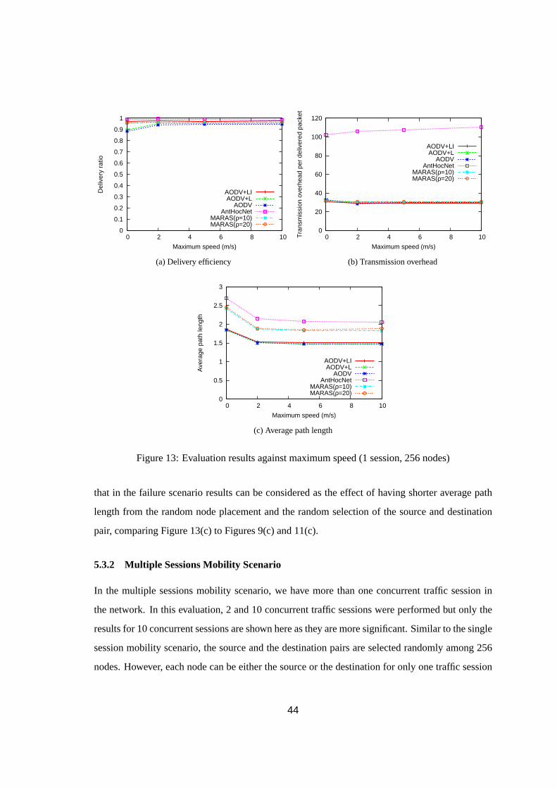
0
0.1
0.2
0.3
0.4
0.5
0.6
0.7
0.8
0.9
1
0 2 4 6 8 10
Del
iver
y ra
tio
Maximum speed (m/s)
AODV+LIAODV+L
AODVAntHocNet
MARAS(ρ=10)MARAS(ρ=20)
(a) Delivery efficiency
0
20
40
60
80
100
120
0 2 4 6 8 10Tra
nsm
issi
on o
verh
ead
per
deliv
ered
pac
ket
Maximum speed (m/s)
AODV+LIAODV+L
AODVAntHocNet
MARAS(ρ=10)MARAS(ρ=20)
(b) Transmission overhead
0
0.5
1
1.5
2
2.5
3
0 2 4 6 8 10
Ave
rage
pat
h le
ngth
Maximum speed (m/s)
AODV+LIAODV+L
AODVAntHocNet
MARAS(ρ=10)MARAS(ρ=20)
(c) Average path length
Figure 13: Evaluation results against maximum speed (1 session, 256 nodes)
that in the failure scenario results can be considered as the effect of having shorter average path
length from the random node placement and the random selection of the source and destination
pair, comparing Figure 13(c) to Figures 9(c) and 11(c).
5.3.2 Multiple Sessions Mobility Scenario
In the multiple sessions mobility scenario, we have more than one concurrent traffic session in
the network. In this evaluation, 2 and 10 concurrent traffic sessions were performed but only the
results for 10 concurrent sessions are shown here as they are more significant. Similar to the single
session mobility scenario, the source and the destination pairs are selected randomly among 256
nodes. However, each node can be either the source or the destination for only one traffic session
44

0
0.1
0.2
0.3
0.4
0.5
0.6
0.7
0.8
0.9
1
0 2 4 6 8 10
Del
iver
y ra
tio
Maximum speed (m/s)
AODV+LIAODV+L
AODVAntHocNet
MARAS(ρ=10)MARAS(ρ=20)
(a) Delivery efficiency
1
10
100
1000
10000
100000
0 2 4 6 8 10Tra
nsm
issi
on o
verh
ead
per
deliv
ered
pac
ket
Maximum speed (m/s)
AODV+LIAODV+L
AODVAntHocNet
MARAS(ρ=10)MARAS(ρ=20)
(b) Transmission overhead
0
0.5
1
1.5
2
2.5
3
0 2 4 6 8 10
Ave
rage
pat
h le
ngth
Maximum speed (m/s)
AODV+LIAODV+L
AODVAntHocNet
MARAS(ρ=10)MARAS(ρ=20)
(c) Average path length
Figure 14: Evaluation results against maximum speed (10 sessions, 256 nodes)
to avoid a bottleneck problem.
The delivery efficiency results are shown in Figure 14(a). First, the delivery efficiency of
AntHocNet totally deteriorates in this high traffic load scenario. The reason is quite obvious that
AntHocNet requires very high overhead as seen in the failure scenarios and the single session
mobility scenario of the mobility scenario. Consequently, the loss of control packets is high as the
network is congested with the high level of traffic and AntHocNet cannot perform well in such
situation.
Next, the delivery efficiencies of AODV and AODV+L become much better than in the cases of
the failure scenarios. In contrast, the delivery efficiency of AODV+LI becomes worse. AODV+LI
shows the tendency of degrading performance when the traffic load is increased in the failure sce-
45

0 0.1 0.2 0.3 0.4 0.5 0.6 0.7 0.8 0.9
1
1 2 10
Del
iver
y ra
tio
Number of CBR traffic sessions
AODVMARAS(ρ=10)MARAS(ρ=20)
(a) Delivery efficiency
0
5
10
15
20
25
30
35
1 2 10Tra
nsm
issi
on o
verh
ead
per
deliv
ered
pac
ket
Number of CBR traffic sessions
AODVMARAS(ρ=10)MARAS(ρ=20)
(b) Transmission overhead
Figure 15: Effects of random walk rangeρ in mobility scenarios (maximum speed = 10 m/s)
narios and this result supports that tendency. Unlike AODV+LI, route recovery packets are flooded
from the source in AODV and AODV+L. This mechanism can find the shorter path, according to
the results in Figure 14(c), than flooding the route recovery packets from the point that the link
failure occurs in AODV+LI. As a result, AODV and AODV+L have higher delivery efficiency than
AODV+LI. Comparing AODV and AODV+L, it can be observed that AODV performs better than
AODV+L which means that the correctness of routing information at the intermediate nodes is not
good enough and it is better to let only the destination respond to the route request packet in this
mobility scenario.
Comparing MARAS to AODV, the delivery efficiency of AODV is slightly larger in the sce-
narios where the maximum speed is less than 5 m/s, but MARAS withρ = 10 has slightly higher
delivery efficiency when the maximum speed becomes larger. However, these differences in terms
of both delivery efficiency and overhead between MARAS and AODV are not significant and it
can be concluded that MARAS withρ = 10 has approximately the same level of performance as
AODV in this scenario.
5.4 Discussion on Random Walk Range (ρ) Parameter in MARAS
When the the random walk rangeρ becomes larger, the random walk packets take longer time to
travel in the network and cause more overhead than lower values ofρ. Therefore, the overhead
of MARAS with ρ = 20 has higher overhead than MARAS withρ = 10 as shown in the case of
46

10 traffic sessions in Figure 15(b). Due to the effect of this overhead, the delivery efficiency of
MARAS with ρ = 20 becomes slightly lower than AODV and MARAS withρ = 10, which can
be seen in Figure 15(a). However, the negative effects from this behavior cannot be seen in the
low number of traffic sessions nor in the failure scenarios. The cause for this effect still requires
further investigation in the future.
5.5 Discussion on Adaptability
In this section, we provide a discussion related to the adaptability of MARAS comparing to the
other protocols: AntHocNet and AODV. First of all, we aim at designing MARAS as a general
purpose routing protocol for MANETs. Therefore, we would like to clarify that MARAS is an
adaptive routing protocol in accordance with its purpose in this section.
Both of the reference protocols: AntHocNet and AODV, can be tuned up as special purpose
routing protocols with high efficiency according to the evaluation in their proposals. In [39], there
are many parameters that have effects on the protocol’s behavior and performance. Even though
the previously tuned parameters of AntHocNet are suitable for scenarios in their evaluation, using
the same set of parameters on our scenario gives different results. In our case, AntHocNet has
higher delivery efficiency than AODV and MARAS only when the level of network dynamics and
the level of traffic are low. However, tuning the AntHocNet to be suitable for a certain network
configuration requires a lot of efforts and also depends on the user’s application which is unknown
and may also change over time. In short, AntHocNet does not hold the adaptability that we seek
to have in MARAS.
On the other hand, AODV has many features that can be selected to match the characteristic of
the network and the application that it will serve under. In our evaluation: AODV, AODV+L, and
AODV+LI are used. AODV+LI performs well in the failure scenarios, but worse in the mobility
scenarios. In contrast, AODV does not performs well in the failure scenarios, but performs very
well in the mobility scenarios. In this case, AODV is better than AntHocNet in terms of adapt-
ability which is our main objective. However, it still requires little modifications on deployment
as well as the selection of the appropriate variant of AODV depending on the situation..
In various scenarios, MARAS might not have shown the best delivery efficiency or the lowest
overhead among all evaluated protocols, but it can maintain relatively high performance. It can be
applied to every scenario in our evaluation with sufficiently high performance without changing
47

any parameters. Moreover, the current parameters we used for MARAS are chosen empirically
and may not even be the optimal ones. Therefore, it may be possible to further improve the
performance of MARAS by exhaustively studying the impact of all parameters, e.g.ρ, β, γ. In
other words, it can adapt to various network characteristics, various levels of traffic, etc. Therefore,
it can be concluded that MARAS is an adaptive general purpose routing protocol for MANETs.
48

6 Conclusion and Future Work
In this thesis, we present MARAS, an biologically-inspired and adaptive routing protocol for
MANETs. For each node operating with this protocol, a next hop selection is performed using
the attractor selection mechanism. This mechanism is inspired from cell biology from which it
inherits the ability to react to a continuously changing environment. The attractor selection mech-
anism is formulated by nonlinear stochastic differential equations with a control factor, called ac-
tivity, which controls the influence of randomness in the selection process. This protocol reactively
establishes the route between the source and the destination and maintains it by using feedback
packets for each successfully delivered packet at the destination. The feedback packet evaluates
the route that the data packet has taken and updates the activity at each node in the route by using
the hop count information, allowing the route to react to changes in the network, e.g., node fail-
ures and mobility, without creating additional control overhead on changes. As a result, MARAS
achieves a higher delivery efficiency and a lower overhead than other well-studied MANET rout-
ing protocols, AODV and AntHocNet, because of its adaptability to frequent failures. Moreover,
when the node density increases, the overhead of MARAS remains almost constant and the deliv-
ery efficiency decreases slower than AODV by which we conclude that MARAS is more scalable.
Additionally, MARAS is capable of maintaining its performance throughout all the evaluated sce-
narios in this study without the need of fine-tuning the parameters to adapt to new conditions as in
other protocols. Therefore, it is concluded that MARAS is suitable as an adaptive general purpose
routing protocol for MANETs.
In the evaluation, a lower overhead of MARAS has been observed in spite of the longer path,
leading to the assumption that the stochastic behavior of MARAS might be capable of avoiding the
congested and unstable links in contrast to the persistent routing based only on the shortest paths
in AODV. As future work, we are interested in studying if MARAS is suitable not only for route
selection but also the traffic management functionality. Moreover, we would like to investigate
the effects of parameters of MARAS, i.e.,ρ, β, andγ, to be able to fine-tune the performance
of MARAS. We expect that once the influences of the parameters on the behavior of MARAS
have been well studied, we can even further improve the performance of MARAS for specific
applications or environments in addition to its general purpose adaptability.
49

Acknowledgments
This thesis would never be accomplished without the support of many people. First, I would
like to express my gratitude to my supervisor, Professor Masayuki Murata, who has always given
me invaluable comments and encouraged me through the hardship of the research. Moreover, I
would like to show my deepest appreciation to Associate Professor Naoki Wakamiya who always
devotes himself to guiding my research and gives me priceless advice. Without his understanding
and support, I would never be able to complete the master’s course.
I would like to particularly thank Specially Appointed Associate Professor Kenji Leibnitz for
his precious time discussing various topics with me. He does not only inspire me with many ideas
but also continually shows his care and understanding. Furthermore, I am greatly indebted to his
effort in proofreading my papers, including this thesis.
Furthermore, I would like to show my gratitude to Associate Professor Go Hasegawa, As-
sistant Professor Shin’ichi Arakawa, and Assistant Professor Yuichi Ohsita for their suggestions
on my research. Also, I must acknowledge Professor Koso Murakami, Professor Makoto Imase,
Professor Teruo Higashino, and Professor Hirotaka Nakano for their comments on this study since
the beginning of master’s course until the final presentation of this thesis.
I am also grateful to the Ministry of Education, Culture, Sports, Science and Technology
(MEXT) for the financial support throughout the master’s course.
Finally, I would like to seize this opportunity to express my personal appreciation to my most
important persons—my family. No words of gratitude would be adequate to their priceless emo-
tional support and love. Thank you for always being there for me.
50

References
[1] M. S. Memon, M. Hashmani, and N. A. Memon, “A review of uniqueness and variations in
throughput due to performance parameters of simulators on MANET routing protocols,” in
Proceedings of the 7th WSEAS International Conference on Electronics, Hardware, Wireless
and Optical Communications (EHAC), pp. 202–208, Feb. 2008.
[2] M. Abolhasan, T. Wysocki, and E. Dutkiewicz, “A review of routing protocols for mobile ad
hoc networks,”Ad Hoc Networks, vol. 2, pp. 1–22, Jan. 2004.
[3] C. Perkins and P. Bhagwat, “Highly dynamic destination-sequenced distance-vector rout-
ing (DSDV) for mobile computers,” inProceedings of the Conference on Communications
Architectures, Protocols and Applications (SIGCOMM), pp. 234–244, Aug. 1994.
[4] T. H. Clausen and P. Jacquet, “Optimized link state routing protocol (OLSR).” RFC 3626,
Oct. 2003.
[5] D. B. Johnson, D. A. Maltz, and J. Broch, “DSR: the dynamic source routing protocol for
multihop wireless ad hoc networks,”Ad Hoc Networking, pp. 139–172, Jan. 2001.
[6] C. Perkins, E. Belding-Royer, and S. Das, “Ad hoc on-demand distance vector (AODV)
routing.” RFC 3561, July 2003.
[7] M. Pearlman and Z. Haas, “Determining the optimal configuration for the zone routing pro-
tocol,” IEEE Journal on Selected Areas in Communications, vol. 17, pp. 1395–1414, Aug.
1999.
[8] M. Joa-Ng and I.-T. Lu, “A peer-to-peer zone-based two-level link state routing for mobile ad
hoc networks,”IEEE Journal on Selected Areas in Communications, vol. 17, pp. 1415–1425,
Aug. 1999.
[9] F. D. Rango, J.-C. Cano, M. Fotino, C. Calafate, P. Manzoni, and S. Marano, “OLSR vs
DSR: A comparative analysis of proactive and reactive mechanisms from an energetic point
of view in wireless ad hoc networks,”Computer Communications, vol. 31, pp. 3843–3854,
Oct. 2008.
51

[10] C. Perkins, E. Royer, S. Das, and M. Marina, “Performance comparison of two on-demand
routing protocols for ad hoc networks,”IEEE Personal Communications, vol. 8, pp. 16–28,
Feb. 2001.
[11] E. Borgia and F. Delmastro, “Effects of unstable links on AODV performance in real
testbeds,”EURASIP Journal on Wireless Communications and Networking, vol. 2007,
pp. 32(1–14), Jan. 2007.
[12] E. Bonabeau, M. Dorigo, and G. Theraulaz,Swarm Intelligence: From Natural to Artificial
Systems. Oxford University Press, 1999.
[13] M. Dorigo, G. Di Caro, and L. M. Gambardella, “Ant algorithms for discrete optimization,”
Artificial Life, vol. 5, pp. 137–172, Apr. 1999.
[14] G. Di Caro, F. Ducatelle, and L. Gambardella, “AntHocNet: An adaptive nature-inspired
algorithm for routing in mobile ad hoc networks,”European Transactions on Telecommuni-
cations, vol. 16, pp. 443–455, Sept. 2005.
[15] H. Wedde, M. Farooq, T. Pannenbaecker, B. Vogel, C. Mueller, J. Meth, and R. Jeruschkat,
“BeeAdHoc: an energy efficient routing algorithm for mobile ad hoc networks inspired by
bee behavior,” inProceedings of the Genetic and Evolutionary Computation Conference
(GECCO), pp. 153–160, June 2005.
[16] J. Wang, E. Osagie, P. Thulasiraman, and R. K. Thulasiram, “HOPNET: A hybrid ant
colony optimization routing algorithm for mobile ad hoc network,”Ad Hoc Networks, vol. 7,
pp. 690–705, June 2009.
[17] K. Leibnitz, N. Wakamiya, and M. Murata, “Self-adaptive ad-hoc/sensor network routing
with attractor-selection,” inProceedings of the IEEE Global Telecommunications Conference
(GLOBECOM), pp. 1–5, Nov. 2006.
[18] K. Leibnitz, N. Wakamiya, and M. Murata, “A bio-inspired robust routing protocol for mo-
bile ad hoc networks,” inProceedings of the 16th International Conference on Computer
Communications and Networks (ICCCN), pp. 321–326, Aug. 2007.
[19] Scalable Network Technologies, Inc., “QualNet 4.0.” Available athttp://www.
scalable-networks.com/products/qualnet/ .
52

[20] J. Wang and S. Lee, “A performance comparison of swarm intelligence inspired routing
algorithms for MANETs,” inProceedings of the International Conference on Computational
Science and Its Applications (ICCSA), pp. 432–442, Mar. 2009.
[21] S. Murthy and J. J. Garcia-Luna-Aceves, “An efficient routing protocol for wireless net-
works,” ACM/Baltzer Journal on Mobile Networks and Applications, Special Issue on Rout-
ing in Mobile Communication Networks, vol. 1, pp. 183–197, Oct. 1996.
[22] G. Pei, M. Gerla, and T.-W. Chen, “Fisheye state routing in mobile ad hoc networks,” in
Proceedings of the ICDCS Workshop on Wireless Networks and Mobile Computing (ICDCS),
pp. D71–D78, Apr. 2000.
[23] G. Pei, M. Gerla, and T.-W. Chen, “Fisheye state routing: a routing scheme for ad hoc wire-
less networks,” inProceedings of the IEEE International Conference on Communications
(ICC), vol. 1, pp. 70–74, June 2000.
[24] T.-W. Chen and M. Gerla, “Global state routing: A new routing scheme for ad-hoc wireless
networks,” inProceedings of IEEE International Communications Conference (ICC), vol. 1,
pp. 171–175, June 1998.
[25] C. Adjih, E. Baccelli, T. H. Clausen, P. Jacquet, and G. Rodolakis, “Fish eye OLSR scaling
properties,”IEEE Journal on Communications Networks, Special Issue on Ad Hoc Network-
ing, vol. 6, pp. 343–351, Dec. 2004.
[26] J. Chen, Y.-Z. Lee, D. Maniezzo, and M. Gerla, “Performance comparison of AODV and
OFLSR in wireless mesh networks,” inProceedings of the IFIP Fifth Annual Mediterranean
Ad Hoc Networking Workshop (Med-Hoc-Net), pp. 271–278, June 2006.
[27] S. Singh, S. S. Sran, and T. Chand, “Performance comparison of AODV, OLSR and OFLSR
in wireless mesh networks,” inProceedings of the 2nd National Conference on Challenges
& Opportunities in Information Technology (COIT), pp. 122–125, Mar. 2008.
[28] C.-K. Toh, “Associativity-based routing for ad-hoc mobile networks,”Wireless Personal
Communications Journal, Special Issue on Mobile Networking and Computing Systems,
vol. 4, pp. 103–139, Mar. 1997.
53

[29] G. Di Caro and M. Dorigo, “AntNet: distributed stigmergetic control for communications
networks,”Journal of Artificial Intelligence Research, vol. 9, pp. 317–365, Aug. 1998.
[30] M. Gunes, U. Sorges, and I. Bouazizi, “ARA - the ant-colony based routing algorithm for
MANETs,” in Proceedings of the 2002 International Conference on Parallel Processing
Workshops (ICPPW), pp. 79–85, Aug. 2002.
[31] R. Martin and W. Stephen, “Termite: A swarm intelligent routing algorithm for mobile
wireless ad-hoc networks,”Stigmergic Optimization, Studies in Computational Intelligence,
pp. 155–184, Oct. 2006.
[32] A. Kashiwagi, I. Urabe, K. Kaneko, and T. Yomo, “Adaptive response of a gene network to
environmental changes by fitness-induced attractor selection,”PLoS ONE, vol. 1, pp. e49(1–
10), Dec. 2006.
[33] C. Avin and C. Brito, “Efficient and robust query processing in dynamic environments using
random walk techniques,” inProceedings of the 3rd International Symposium on Information
Processing in Sensor Networks (IPSN), pp. 277–286, Apr. 2004.
[34] B. Selman, H. Kautz, and B. Cohen, “Noise strategies for improving local search,” inPro-
ceedings of the National Conference on Artificial Intelligence (AAAI), pp. 337–343, July
1994.
[35] C. Perkins, E. Royer, and S. Das, “Ad hoc on-demand distance vector routing, draft-ietf-
manet-aodv-08.txt,”IETF MANET Working Group, Mar. 2001.
[36] F. Ducatelle, “AntHocNet4.zip: code for the use of AntHocNet in the QualNet 4.0 net-
work simulator.” Available athttp://www.idsia.ch/ ∼frederick/anthocnet/
anthocnet.html .
[37] C. Perkins, E. Royer, and S. Das, “Ad hoc on-demand distance vector routing, draft-ietf-
manet-aodv-09.txt,”IETF MANET Working Group, Nov. 2001.
[38] M. I. M. Saad and Z. A. Zukarnain, “Performance analysis of random-based mobility models
in MANET routing protocol,”European Journal of Scientific Research, vol. 32, June 2009.
54

[39] F. Ducatelle,Adaptive Routing in Ad Hoc Wireless Multi-hop Networks. PhD thesis, Univer-
sita della Svizzera italiana, May 2007.
55