mastering sketching: adversarial augmentation for ...ess/publications/simoserratog2018.pdf ·...

Mastering Sketching: Adversarial Augmentation for StructuredPrediction

EDGAR SIMO-SERRA, Waseda University

SATOSHI IIZUKA, Waseda University

HIROSHI ISHIKAWA, Waseda University

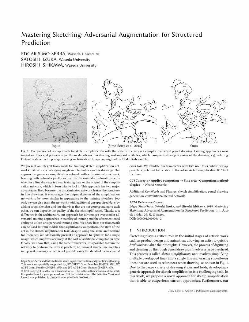
Input [Simo-Serra et al. 2016] Ours

Fig. 1. Comparison of our approach for sketch simplification with the state of the art on a complex real world pencil drawing. Existing approaches miss

important lines and preserve superfluous details such as shading and support scribbles, which hampers further processing of the drawing, e.g., coloring.

Output is shown with post-processing vectorization. Image copyrighted by Eisaku Kubonouchi.

We present an integral framework for training sketch simplification net-

works that convert challenging rough sketches into clean line drawings. Our

approach augments a simplification network with a discriminator network,

training both networks jointly so that the discriminator network discerns

whether a line drawing is a real training data or the output of the simplifi-

cation network, which in turn tries to fool it. This approach has two major

advantages: first, because the discriminator network learns the structure

in line drawings, it encourages the output sketches of the simplification

network to be more similar in appearance to the training sketches. Sec-

ond, we can also train the networks with additional unsupervised data: by

adding rough sketches and line drawings that are not corresponding to each

other, we can improve the quality of the sketch simplification. Thanks to a

difference in the architecture, our approach has advantages over similar ad-

versarial training approaches in stability of training and the aforementioned

ability to utilize unsupervised training data. We show how our framework

can be used to train models that significantly outperform the state of the

art in the sketch simplification task, despite using the same architecture

for inference. We additionally present an approach to optimize for a single

image, which improves accuracy at the cost of additional computation time.

Finally, we show that, using the same framework, it is possible to train the

network to perform the inverse problem, i.e., convert simple line sketches

into pencil drawings, which is not possible using the standard mean squared

Edgar Simo-Serra and Satoshi Iizuka assert equal contribution and joint first authorship.This work was partially supported by JST CREST Grant Number JPMJCR14D1, JSTACT-I Grant Number JPMJPR16UD, and JST ACT-I Grant Number JPMJPR16U3.© 2018 Copyright held by the owner/author(s). This is the author’s version of the work.It is posted here for your personal use. Not for redistribution. The definitive Version ofRecord was published in , https://doi.org/0000001.0000001_2.

error loss. We validate our framework with two user tests, where our ap-

proach is preferred to the state of the art in sketch simplification 88.9% of

the time.

CCSConcepts: •Applied computing→ Fine arts; •Computingmethod-

ologies→ Neural networks;

Additional Key Words and Phrases: sketch simplification, pencil drawing

generation, convolutional neural network

ACM Reference format:

Edgar Simo-Serra, Satoshi Iizuka, and Hiroshi Ishikawa. 2018. Mastering

Sketching: Adversarial Augmentation for Structured Prediction. 1, 1, Arti-

cle 1 (May 2018), 13 pages.

DOI: 0000001.0000001_2

1 INTRODUCTION

Sketching plays a critical role in the initial stages of artistic work

such as product design and animation, allowing an artist to quickly

draft and visualize their thoughts. However, the process of digitizing

and cleaning up the rough pencil drawings involves a large overhead.

This process is called sketch simplification, and involves simplifying

multiple overlapped lines into a single line and erasing superfluous

lines that are used as references when drawing, as shown in Fig. 1.

Due to the large variety of drawing styles and tools, developing a

generic approach for sketch simplification is a challenging task. In

this work, we propose a novel approach for sketch simplification

that is able to outperform current approaches. Furthermore, our

, Vol. 1, No. 1, Article 1. Publication date: May 2018.

https://doi.org/0000001.0000001_2

1:2 • Edgar Simo-Serra, Satoshi Iizuka, and Hiroshi Ishikawa

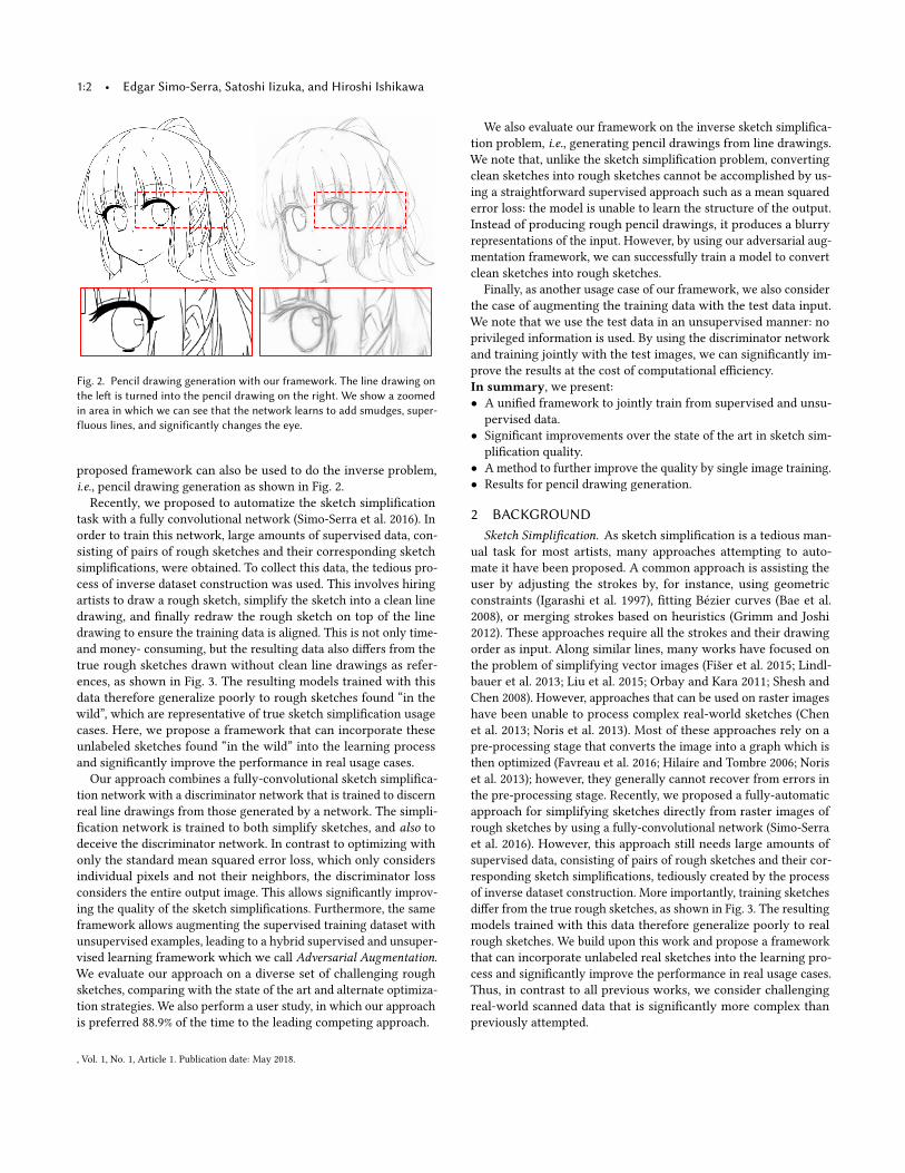
Fig. 2. Pencil drawing generation with our framework. The line drawing on

the le� is turned into the pencil drawing on the right. We show a zoomed

in area in which we can see that the network learns to add smudges, super-

fluous lines, and significantly changes the eye.

proposed framework can also be used to do the inverse problem,

i.e., pencil drawing generation as shown in Fig. 2.

Recently, we proposed to automatize the sketch simplification

task with a fully convolutional network (Simo-Serra et al. 2016). In

order to train this network, large amounts of supervised data, con-

sisting of pairs of rough sketches and their corresponding sketch

simplifications, were obtained. To collect this data, the tedious pro-

cess of inverse dataset construction was used. This involves hiring

artists to draw a rough sketch, simplify the sketch into a clean line

drawing, and finally redraw the rough sketch on top of the line

drawing to ensure the training data is aligned. This is not only time-

and money- consuming, but the resulting data also differs from the

true rough sketches drawn without clean line drawings as refer-

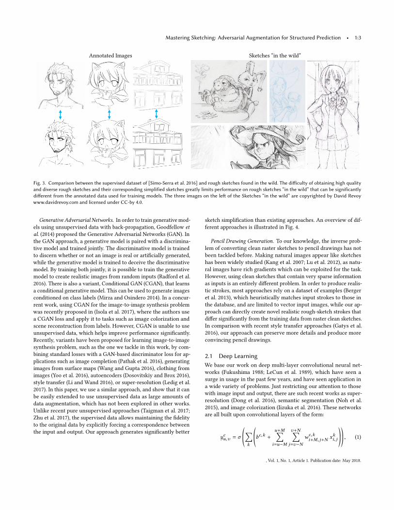
ences, as shown in Fig. 3. The resulting models trained with this

data therefore generalize poorly to rough sketches found “in the

wild”, which are representative of true sketch simplification usage

cases. Here, we propose a framework that can incorporate these

unlabeled sketches found “in the wild” into the learning process

and significantly improve the performance in real usage cases.

Our approach combines a fully-convolutional sketch simplifica-

tion network with a discriminator network that is trained to discern

real line drawings from those generated by a network. The simpli-

fication network is trained to both simplify sketches, and also to

deceive the discriminator network. In contrast to optimizing with

only the standard mean squared error loss, which only considers

individual pixels and not their neighbors, the discriminator loss

considers the entire output image. This allows significantly improv-

ing the quality of the sketch simplifications. Furthermore, the same

framework allows augmenting the supervised training dataset with

unsupervised examples, leading to a hybrid supervised and unsuper-

vised learning framework which we call Adversarial Augmentation.

We evaluate our approach on a diverse set of challenging rough

sketches, comparing with the state of the art and alternate optimiza-

tion strategies. We also perform a user study, in which our approach

is preferred 88.9% of the time to the leading competing approach.

We also evaluate our framework on the inverse sketch simplifica-

tion problem, i.e., generating pencil drawings from line drawings.

We note that, unlike the sketch simplification problem, converting

clean sketches into rough sketches cannot be accomplished by us-

ing a straightforward supervised approach such as a mean squared

error loss: the model is unable to learn the structure of the output.

Instead of producing rough pencil drawings, it produces a blurry

representations of the input. However, by using our adversarial aug-

mentation framework, we can successfully train a model to convert

clean sketches into rough sketches.

Finally, as another usage case of our framework, we also consider

the case of augmenting the training data with the test data input.

We note that we use the test data in an unsupervised manner: no

privileged information is used. By using the discriminator network

and training jointly with the test images, we can significantly im-

prove the results at the cost of computational efficiency.

In summary, we present:

• A unified framework to jointly train from supervised and unsu-

pervised data.

• Significant improvements over the state of the art in sketch sim-

plification quality.

• Amethod to further improve the quality by single image training.

• Results for pencil drawing generation.

2 BACKGROUND

Sketch Simplification. As sketch simplification is a tedious man-

ual task for most artists, many approaches attempting to auto-

mate it have been proposed. A common approach is assisting the

user by adjusting the strokes by, for instance, using geometric

constraints (Igarashi et al. 1997), fitting Bézier curves (Bae et al.

2008), or merging strokes based on heuristics (Grimm and Joshi

2012). These approaches require all the strokes and their drawing

order as input. Along similar lines, many works have focused on

the problem of simplifying vector images (Fišer et al. 2015; Lindl-

bauer et al. 2013; Liu et al. 2015; Orbay and Kara 2011; Shesh and

Chen 2008). However, approaches that can be used on raster images

have been unable to process complex real-world sketches (Chen

et al. 2013; Noris et al. 2013). Most of these approaches rely on a

pre-processing stage that converts the image into a graph which is

then optimized (Favreau et al. 2016; Hilaire and Tombre 2006; Noris

et al. 2013); however, they generally cannot recover from errors in

the pre-processing stage. Recently, we proposed a fully-automatic

approach for simplifying sketches directly from raster images of

rough sketches by using a fully-convolutional network (Simo-Serra

et al. 2016). However, this approach still needs large amounts of

supervised data, consisting of pairs of rough sketches and their cor-

responding sketch simplifications, tediously created by the process

of inverse dataset construction. More importantly, training sketches

differ from the true rough sketches, as shown in Fig. 3. The resulting

models trained with this data therefore generalize poorly to real

rough sketches. We build upon this work and propose a framework

that can incorporate unlabeled real sketches into the learning pro-

cess and significantly improve the performance in real usage cases.

Thus, in contrast to all previous works, we consider challenging

real-world scanned data that is significantly more complex than

previously attempted.


Mastering Sketching: Adversarial Augmentation for Structured Prediction • 1:3

Annotated Images Sketches “in the wild”

Fig. 3. Comparison between the supervised dataset of [Simo-Serra et al. 2016] and rough sketches found in the wild. The difficulty of obtaining high quality

and diverse rough sketches and their corresponding simplified sketches greatly limits performance on rough sketches “in the wild” that can be significantly

different from the annotated data used for training models. The three images on the le� of the Sketches “in the wild” are copyrighted by David Revoy

www.davidrevoy.com and licensed under CC-by 4.0.

Generative Adversarial Networks. In order to train generative mod-

els using unsupervised data with back-propagation, Goodfellow et

al. (2014) proposed the Generative Adversarial Networks (GAN). In

the GAN approach, a generative model is paired with a discrimina-

tive model and trained jointly. The discriminative model is trained

to discern whether or not an image is real or artificially generated,

while the generative model is trained to deceive the discriminative

model. By training both jointly, it is possible to train the generative

model to create realistic images from random inputs (Radford et al.

2016). There is also a variant, Conditional GAN (CGAN), that learns

a conditional generative model. This can be used to generate images

conditioned on class labels (Mirza and Osindero 2014). In a concur-

rent work, using CGAN for the image-to-image synthesis problem

was recently proposed in (Isola et al. 2017), where the authors use

a CGAN loss and apply it to tasks such as image colorization and

scene reconstruction from labels. However, CGAN is unable to use

unsupervised data, which helps improve performance significantly.

Recently, variants have been proposed for learning image-to-image

synthesis problem, such as the one we tackle in this work, by com-

bining standard losses with a GAN-based discriminator loss for ap-

plications such as image completion (Pathak et al. 2016), generating

images from surface maps (Wang and Gupta 2016), clothing from

images (Yoo et al. 2016), autoencoders (Dosovitskiy and Brox 2016),

style transfer (Li and Wand 2016), or super-resolution (Ledig et al.

2017). In this paper, we use a similar approach, and show that it can

be easily extended to use unsupervised data as large amounts of

data augmentation, which has not been explored in other works.

Unlike recent pure unsupervised approaches (Taigman et al. 2017;

Zhu et al. 2017), the supervised data allows maintaining the fidelity

to the original data by explicitly forcing a correspondence between

the input and output. Our approach generates significantly better

sketch simplification than existing approaches. An overview of dif-

ferent approaches is illustrated in Fig. 4.

Pencil Drawing Generation. To our knowledge, the inverse prob-

lem of converting clean raster sketches to pencil drawings has not

been tackled before. Making natural images appear like sketches

has been widely studied (Kang et al. 2007; Lu et al. 2012), as natu-

ral images have rich gradients which can be exploited for the task.

However, using clean sketches that contain very sparse information

as inputs is an entirely different problem. In order to produce realis-

tic strokes, most approaches rely on a dataset of examples (Berger

et al. 2013), which heuristically matches input strokes to those in

the database, and are limited to vector input images, while our ap-

proach can directly create novel realistic rough-sketch strokes that

differ significantly from the training data from raster clean sketches.

In comparison with recent style transfer approaches (Gatys et al.

2016), our approach can preserve more details and produce more

convincing pencil drawings.

2.1 Deep Learning

We base our work on deep multi-layer convolutional neural net-

works (Fukushima 1988; LeCun et al. 1989), which have seen a

surge in usage in the past few years, and have seen application in

a wide variety of problems. Just restricting our attention to those

with image input and output, there are such recent works as super-

resolution (Dong et al. 2016), semantic segmentation (Noh et al.

2015), and image colorization (Iizuka et al. 2016). These networks

are all built upon convolutional layers of the form:

ycu,v = σ©«∑k

©«bc,k +

u+M∑i=u−M

v+N∑j=v−N

wc,ki+M, j+N

xki, jª®¬ª®¬, (1)


http://www.davidrevoy.com



where for a (2M + 1) × (2N + 1) convolution kernel, each output

channel c and coordinates (u,v), the output value ycu,v is computed

as an affine transformation of the input pixel xku,v for all input

channels k with a shared weight matrix formed by wc,k and bias

value bc,k that is run through a non-linear activation function σ (·).

The most widely used non-linear activation function is the Rectified

Linear Unit (ReLU) where σ (x) = max(0,x) (Nair and Hinton 2010).

These layers are a series of learnable filters withw and b being

the learnable parameters. In order to train a network, a dataset con-

sisting of pairs of input and their corresponding ground truth (x ,y∗)

are used in conjunction with a loss function L(y,y∗) that measures

the error between the output y of the network and the ground truth

y∗. This error is used to update the learnable parameters with the

backpropagation algorithm (Rumelhart et al. 1986). In this work we

also consider the scenario in which not all data is necessarily in the

form of pairs (x ,y∗), but can also be in the form of single samples x

and y∗ that are not corresponding pairs.

Our work is based on fully-convolutional neural network models

that can be applied to images of any resolution. These networks

generally follow an encoder-decoder architecture, in which the

first layers of the network have an increased stride to lower the

resolution of the input layer. At lower resolutions, the subsequent

layers are able to process larger regions of the input image: for

instance, a 3 × 3-pixel convolution on an image at half resolution is

computed with a 5× 5-pixel area of the original image. Additionally,

by processing at lower resolutions, both the memory requirements

and computation times are significantly decreased. In this paper,

we base our network model on that of (Simo-Serra et al. 2016) and

show that we can greatly improve the performance of the resulting

model by using a significantly improved learning approach.

3 ADVERSARIAL AUGMENTATION

We present adversarial augmentation, which is the fusion of unsuper-

vised and adversarial training focused on the purpose of augmenting

existing networks for structured prediction tasks. An overview of

our approach compared with different training approaches can be

seen in Fig. 4. Similar to Generative Adversarial Networks (GAN) (Good-

fellow et al. 2014), we employ a discriminator network that attempts

to distinguish whether an image comes from real data or is the out-

put of another network. Unlike in the case of standard supervised

losses such as the Mean Squared Error (MSE), with the discrimina-

tor network the output is encouraged to have a global consistency

similar to the training images. Although similar approaches have

been proposed (Ledig et al. 2017; Pathak et al. 2016; Zhou and Berg

2016), they have focused exclusively on supervised training. In this

work we focus on training with additional unlabeled examples, and

show that this both increases the performance and generalization.

An overview of our framework can be seen in Fig. 5.

While this work focuses on sketch simplification, the presented

approach is general and applicable to other structured prediction

problems, such as semantic segmentation or saliency detection.

3.1 The GAN Framework

The purpose of Generative Adversarial Network (GAN) (Goodfellow

et al. 2014) is, given a training set of samples, estimating a generative

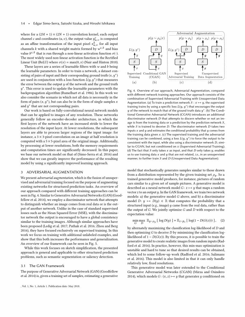
Fig. 4. Overview of our approach, Adversarial Augmentation, compared

with different network training approaches. Our approach consists of the

combination of Supervised Adversarial Training with Unsupervised Data

Augmentation. (a) To train a prediction network S : x 7→ y , the supervised

training trains by using a specific loss L(y, y∗) that encourages the output

y of the network to match that of the ground truth data y∗. (b) The Condi-

tional Generative Adversarial Network (CGAN) introduces an additional

discriminator network D that a�empts to discern whether or not an im-

age is from the training data or a prediction by the prediction network S ,

while S is trained to deceive D . The discriminator network D takes two

inputs x and y and estimates the conditional probability that y comes from

the training data given x . (c) The supervised training and the adversarial

training can be combined, using a loss L(y, y∗) to force the output to be

consistent with the input, while also using a discriminator network D , simi-

lar to CGAN, but not conditioned on x (Supervised Adversarial Training).

(d) The fact that S only takes x as input, and that D only takes y , enables

us to use training data x and y that are not related, i.e., in an unsupervised

manner, to further train S and D (Unsupervised Data Augmentation).

model that stochastically generates samples similar to those drawn

from a distribution represented by the given training set ρy . So a

trained generative model produces, for instance, pictures of random

cars similar to a given set of sample pictures. A generative model is

described as a neural network modelG : z 7→ y that maps a random

vector z to an outputy. In the GAN framework, we train two network

models: a) the generative model G above, and b) a discriminator

model D : y 7→ D(y) ∈ R that computes the probability that a

structured input (e.g., image) y came from the real data, rather than

the output of G. We jointly optimize G and D with respect to the

expectation value:

minG

maxDEy∼ρy [ logD(y) ] + Ez∼pz [ log(1 − D(G(z))) ] , (2)

by alternately maximizing the classification log-likelihood of D and

then optimizingG to deceive D by minimizing the classification log-

likelihood of 1 − D(G(z)). By this process, it is possible to train the

generative model to create realistic images from random inputs (Rad-

ford et al. 2016). In practice, however, this min-max optimization is

unstable and hard to tune so that desired results can be obtained,

which led to some follow-up work (Radford et al. 2016; Salimans

et al. 2016). This model is also limited in that it can only handle

relatively low, fixed resolutions.

This generative model was later extended to the Conditional

Generative Adversarial Networks (CGAN) (Mirza and Osindero

2014), which models G : (x , z) 7→ y that generates y conditioned on



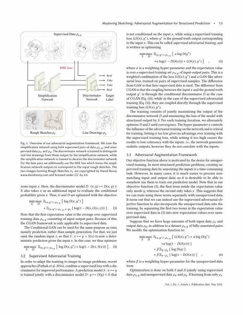
Rough Sketches

Supervised Data

Discriminator

Network

Line Drawings

Simplification

Network

Real

Real

Fake

Fake

Target

Label

MSE loss

Fig. 5. Overview of our adversarial augmentation framework. We train the

simplification network using both supervised pairs of data ρx,y , and unsu-

pervised data ρx and ρy . The discriminator network is trained to distinguish

real line drawings from those output by the simplification network, while

the simplification network is trained to deceive the discriminator network.

For the data pairs we additionally use the MSE loss which forces the simpli-

fication network outputs to correspond to the input rough sketches. The

two images forming Rough Sketches σx are copyrighted by David Revoy


some input x . Here, the discriminator model D : (x ,y) 7→ D(x ,y) ∈

R also takes x as an additional input to evaluate the conditional

probability given x . Thus,G and D are optimized with the objective:

minG

maxDE(x,y∗)∼ρx,y

[logD(x ,y∗)

]+ E(x,y∗)∼ρx,y,z∼pz [ log(1 − D(x ,G(x , z))) ] . (3)

Note that the first expectation value is the average over supervised

training data ρx,y consisting of input-output pairs. Because of this,

the CGAN framework is only applicable to supervised data.

The Conditional GAN can be used for the same purpose as ours,

namely prediction, rather than sample generation. For that, we just

omit the random input z, so that S : x 7→ y = S(x) is now a deter-

ministic prediction given the input x . In this case, we thus optimize:

minS


[logD(x ,y∗) + log(1 − D(x , S(x)))

]. (4)

3.2 Supervised Adversarial Training

In order to adapt the training to image-to-image problems, recent

approaches (Pathak et al. 2016), combine a supervised loss with a dis-

criminator for improved performance. A prediction model S : x 7→ y

is trained jointly with a discriminator model D : y 7→ D(y) ∈ R that

is not conditioned on the input x , while using a supervised training

loss L(S(x),y∗), where y∗ is the ground truth output corresponding

to the input x . This can be called supervised adversarial training, and

is written as optimizing

minS


[α logD(y∗)

+α log(1 − D(S(x))) + L(S(x),y∗)], (5)

where α is a weighting hyper-parameter and the expectation value

is over a supervised training set ρx,y of input-output pairs. This is a

weighted combination of the loss L(S(x),y∗) and a GAN-like adver-

sarial loss, trained on pairs of supervised samples. The difference

from GAN is that here supervised data is used. The difference from

CGAN is that the coupling between the input x and the ground truth

output y∗ is through the conditional discriminator D in the case

of CGAN (Eq. (4)), while in the case of the supervised adversarial

training (Eq. (5)), they are coupled directly through the supervised

training loss L(S(x),y∗).

The training consists of jointly maximizing the output of the

discriminator network D and minimizing the loss of the model with

structured output by S . For each training iteration, we alternately

optimizeD and S until convergence. The hyper-parameterα controls

the influence of the adversarial training on the network and is critical

for training. Setting α too low gives no advantage over training with

the supervised training loss, while setting it too high causes the

results to lose coherency with the inputs, i.e., the network generates

realistic outputs, however they do not correlate with the inputs.

3.3 Adversarial Augmentation Framework

Our objective function above is motivated by the desire for unsuper-

vised training. In most structured prediction problems, creating su-

pervised training data by annotating the inputs is a time-consuming

task. However, in many cases, it is much easier to procure non-

matching input and output data; so it is desirable to be able to

somehow use them to train our prediction model. Note that in our

objective function (5), the first term inside the expectation value

only needs y, whereas the second only takes x . This suggests that

we can train using these terms separately with unsupervised data.

It turns out that we can indeed use the supervised adversarial ob-

jective function to also incorporate the unsupervised data into the

training, by separating the first two terms in the expectation value

over supervised data in (5) into new expectation values over unsu-

pervised data.

Suppose that we have large amounts of both input data ρx and

output data ρy , in addition to a dataset ρx,y of fully-annotated pairs.

We modify the optimization function to:

minS


[L(S(x),y∗) + α logD(y∗)

+α log(1 − D(S(x))) ]

+ β Ey∼ρy [ logD(y) ]

+ β Ex∼ρx [ log(1 − D(S(x))) ] , (6)

where β is a weighting hyper-parameter for the unsupervised data

term.

Optimization is done on both S and D jointly using supervised

data ρx,y and unsupervised data ρx and ρy . If learning from only ρx





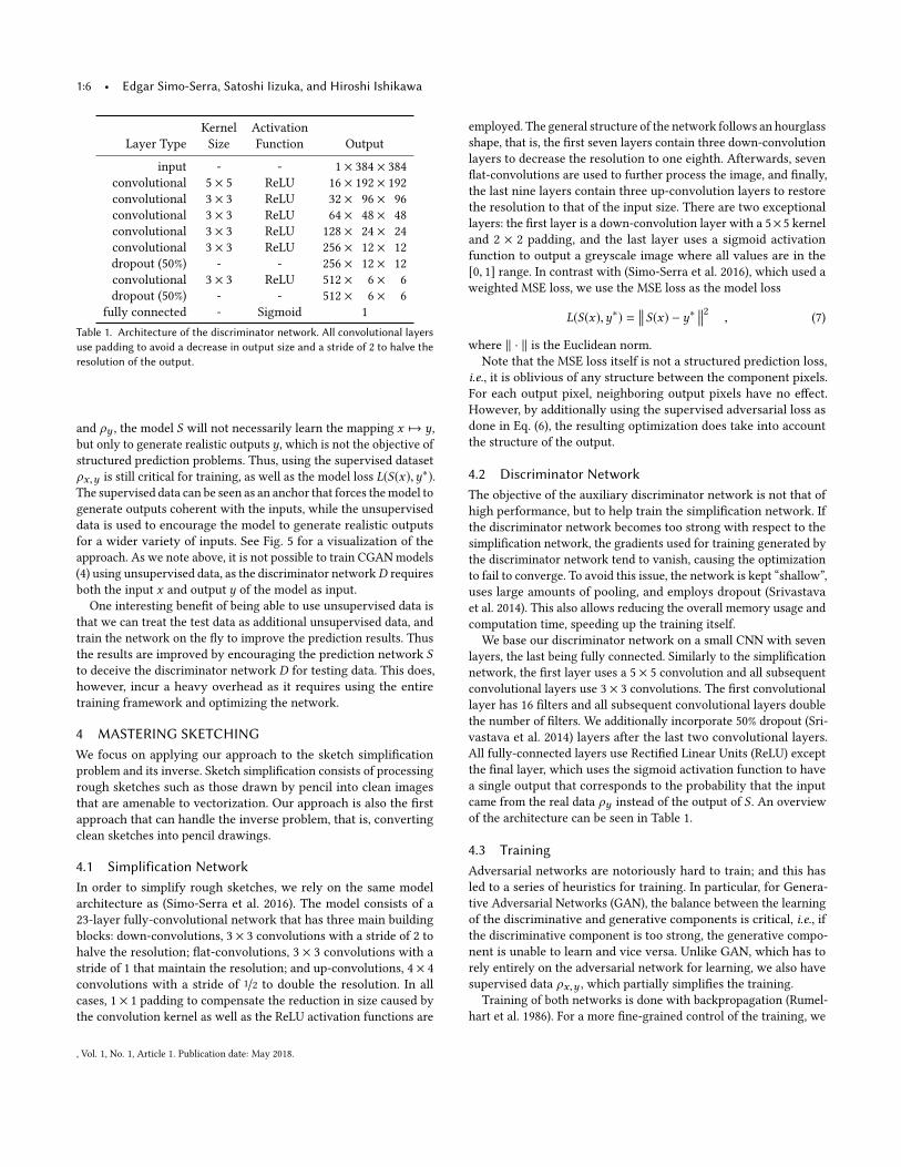
Kernel Activation

Layer Type Size Function Output

input - - 1 × 384 × 384

convolutional 5 × 5 ReLU 16 × 192 × 192





dropout (50%) - - 256 × 12 × 12


dropout (50%) - - 512 × 6 × 6

fully connected - Sigmoid 1

Table 1. Architecture of the discriminator network. All convolutional layers

use padding to avoid a decrease in output size and a stride of 2 to halve the

resolution of the output.

and ρy , the model S will not necessarily learn the mapping x 7→ y,

but only to generate realistic outputs y, which is not the objective of

structured prediction problems. Thus, using the supervised dataset

ρx,y is still critical for training, as well as the model loss L(S(x),y∗).

The supervised data can be seen as an anchor that forces themodel to

generate outputs coherent with the inputs, while the unsupervised

data is used to encourage the model to generate realistic outputs

for a wider variety of inputs. See Fig. 5 for a visualization of the

approach. As we note above, it is not possible to train CGANmodels

(4) using unsupervised data, as the discriminator networkD requires

both the input x and output y of the model as input.

One interesting benefit of being able to use unsupervised data is

that we can treat the test data as additional unsupervised data, and

train the network on the fly to improve the prediction results. Thus

the results are improved by encouraging the prediction network S

to deceive the discriminator network D for testing data. This does,

however, incur a heavy overhead as it requires using the entire

training framework and optimizing the network.

4 MASTERING SKETCHING

We focus on applying our approach to the sketch simplification

problem and its inverse. Sketch simplification consists of processing

rough sketches such as those drawn by pencil into clean images

that are amenable to vectorization. Our approach is also the first

approach that can handle the inverse problem, that is, converting

clean sketches into pencil drawings.

4.1 Simplification Network

In order to simplify rough sketches, we rely on the same model

architecture as (Simo-Serra et al. 2016). The model consists of a

23-layer fully-convolutional network that has three main building

blocks: down-convolutions, 3 × 3 convolutions with a stride of 2 to

halve the resolution; flat-convolutions, 3 × 3 convolutions with a

stride of 1 that maintain the resolution; and up-convolutions, 4 × 4

convolutions with a stride of 1/2 to double the resolution. In all

cases, 1 × 1 padding to compensate the reduction in size caused by

the convolution kernel as well as the ReLU activation functions are

employed. The general structure of the network follows an hourglass

shape, that is, the first seven layers contain three down-convolution

layers to decrease the resolution to one eighth. Afterwards, seven

flat-convolutions are used to further process the image, and finally,

the last nine layers contain three up-convolution layers to restore

the resolution to that of the input size. There are two exceptional

layers: the first layer is a down-convolution layer with a 5× 5 kernel

and 2 × 2 padding, and the last layer uses a sigmoid activation

function to output a greyscale image where all values are in the

[0, 1] range. In contrast with (Simo-Serra et al. 2016), which used a

weighted MSE loss, we use the MSE loss as the model loss

L(S(x),y∗) = S(x) − y∗

2, (7)

where ‖ · ‖ is the Euclidean norm.

Note that the MSE loss itself is not a structured prediction loss,

i.e., it is oblivious of any structure between the component pixels.

For each output pixel, neighboring output pixels have no effect.

However, by additionally using the supervised adversarial loss as

done in Eq. (6), the resulting optimization does take into account

the structure of the output.

4.2 Discriminator Network

The objective of the auxiliary discriminator network is not that of

high performance, but to help train the simplification network. If

the discriminator network becomes too strong with respect to the

simplification network, the gradients used for training generated by

the discriminator network tend to vanish, causing the optimization

to fail to converge. To avoid this issue, the network is kept “shallow”,

uses large amounts of pooling, and employs dropout (Srivastava

et al. 2014). This also allows reducing the overall memory usage and

computation time, speeding up the training itself.

We base our discriminator network on a small CNN with seven

layers, the last being fully connected. Similarly to the simplification

network, the first layer uses a 5 × 5 convolution and all subsequent

convolutional layers use 3 × 3 convolutions. The first convolutional

layer has 16 filters and all subsequent convolutional layers double

the number of filters. We additionally incorporate 50% dropout (Sri-

vastava et al. 2014) layers after the last two convolutional layers.

All fully-connected layers use Rectified Linear Units (ReLU) except

the final layer, which uses the sigmoid activation function to have

a single output that corresponds to the probability that the input

came from the real data ρy instead of the output of S . An overview

of the architecture can be seen in Table 1.

4.3 Training

Adversarial networks are notoriously hard to train; and this has

led to a series of heuristics for training. In particular, for Genera-

tive Adversarial Networks (GAN), the balance between the learning

of the discriminative and generative components is critical, i.e., if

the discriminative component is too strong, the generative compo-

nent is unable to learn and vice versa. Unlike GAN, which has to

rely entirely on the adversarial network for learning, we also have

supervised data ρx,y , which partially simplifies the training.

Training of both networks is done with backpropagation (Rumel-

hart et al. 1986). For a more fine-grained control of the training, we


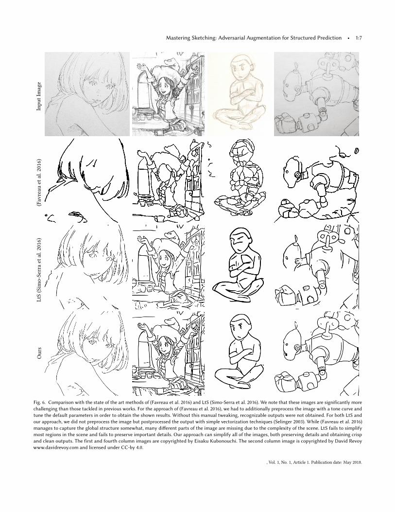
Mastering Sketching: Adversarial Augmentation for Structured Prediction • 1:7InputIm

age

(Favreau

etal.2016)

LtS

(Sim

o-Serra

etal.2016)

Ours

Fig. 6. Comparison with the state of the art methods of (Favreau et al. 2016) and LtS (Simo-Serra et al. 2016). We note that these images are significantly more

challenging than those tackled in previous works. For the approach of (Favreau et al. 2016), we had to additionally preprocess the image with a tone curve and

tune the default parameters in order to obtain the shown results. Without this manual tweaking, recognizable outputs were not obtained. For both LtS and

our approach, we did not preprocess the image but postprocessed the output with simple vectorization techniques (Selinger 2003). While (Favreau et al. 2016)

manages to capture the global structure somewhat, many different parts of the image are missing due to the complexity of the scene. LtS fails to simplify

most regions in the scene and fails to preserve important details. Our approach can simplify all of the images, both preserving details and obtaining crisp

and clean outputs. The first and fourth column images are copyrighted by Eisaku Kubonouchi. The second column image is copyrighted by David Revoy






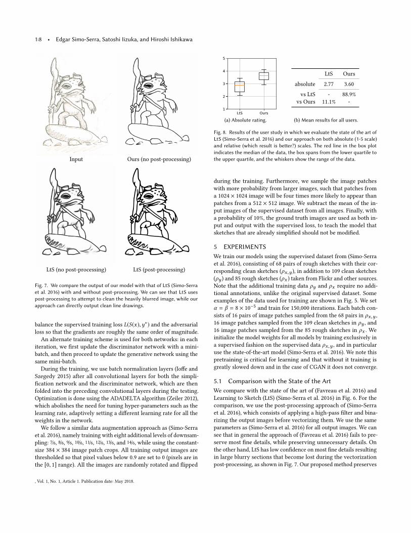
Input Ours (no post-processing)

LtS (no post-processing) LtS (post-processing)

Fig. 7. We compare the output of our model with that of LtS (Simo-Serra

et al. 2016) with and without post-processing. We can see that LtS uses

post-processing to a�empt to clean the heavily blurred image, while our

approach can directly output clean line drawings.

balance the supervised training loss L(S(x),y∗) and the adversarial

loss so that the gradients are roughly the same order of magnitude.

An alternate training scheme is used for both networks: in each

iteration, we first update the discriminator network with a mini-

batch, and then proceed to update the generative network using the

same mini-batch.

During the training, we use batch normalization layers (Ioffe and

Szegedy 2015) after all convolutional layers for both the simpli-

fication network and the discriminator network, which are then

folded into the preceding convolutional layers during the testing.

Optimization is done using the ADADELTA algorithm (Zeiler 2012),

which abolishes the need for tuning hyper-parameters such as the

learning rate, adaptively setting a different learning rate for all the

weights in the network.

We follow a similar data augmentation approach as (Simo-Serra

et al. 2016), namely training with eight additional levels of downsam-

pling: 7/6, 8/6, 9/6, 10/6, 11/6, 12/6, 13/6, and 14/6, while using the constant-

size 384 × 384 image patch crops. All training output images are

thresholded so that pixel values below 0.9 are set to 0 (pixels are in

the [0, 1] range). All the images are randomly rotated and flipped

LtS Ours1

2

3

4

5

(a) Absolute rating.

LtS Ours

absolute 2.77 3.60

vs LtS - 88.9%

vs Ours 11.1% -

(b) Mean results for all users.

Fig. 8. Results of the user study in which we evaluate the state of the art of

LtS (Simo-Serra et al. 2016) and our approach on both absolute (1-5 scale)

and relative (which result is be�er?) scales. The red line in the box plot

indicates the median of the data, the box spans from the lower quartile to

the upper quartile, and the whiskers show the range of the data.

during the training. Furthermore, we sample the image patches

with more probability from larger images, such that patches from

a 1024 × 1024 image will be four times more likely to appear than

patches from a 512 × 512 image. We subtract the mean of the in-

put images of the supervised dataset from all images. Finally, with

a probability of 10%, the ground truth images are used as both in-

put and output with the supervised loss, to teach the model that

sketches that are already simplified should not be modified.

5 EXPERIMENTS

We train our models using the supervised dataset from (Simo-Serra

et al. 2016), consisting of 68 pairs of rough sketches with their cor-

responding clean sketches (ρx,y ), in addition to 109 clean sketches

(ρy ) and 85 rough sketches (ρx ) taken from Flickr and other sources.

Note that the additional training data ρy and ρx require no addi-

tional annotations, unlike the original supervised dataset. Some

examples of the data used for training are shown in Fig. 5. We set

α = β = 8 × 10−5 and train for 150,000 iterations. Each batch con-

sists of 16 pairs of image patches sampled from the 68 pairs in ρx,y ,

16 image patches sampled from the 109 clean sketches in ρy , and

16 image patches sampled from the 85 rough sketches in ρx . We

initialize the model weights for all models by training exclusively in

a supervised fashion on the supervised data ρx,y , and in particular

use the state-of-the-art model (Simo-Serra et al. 2016). We note this

pretraining is critical for learning and that without it training is

greatly slowed down and in the case of CGAN it does not converge.

5.1 Comparison with the State of the Art

We compare with the state of the art of (Favreau et al. 2016) and

Learning to Sketch (LtS) (Simo-Serra et al. 2016) in Fig. 6. For the

comparison, we use the post-processing approach of (Simo-Serra

et al. 2016), which consists of applying a high-pass filter and bina-

rizing the output images before vectorizing them. We use the same

parameters as (Simo-Serra et al. 2016) for all output images. We can

see that in general the approach of (Favreau et al. 2016) fails to pre-

serve most fine details, while preserving unnecessary details. On

the other hand, LtS has low confidence on most fine details resulting

in large blurry sections that become lost during the vectorization

post-processing, as shown in Fig. 7. Our proposed method preserves



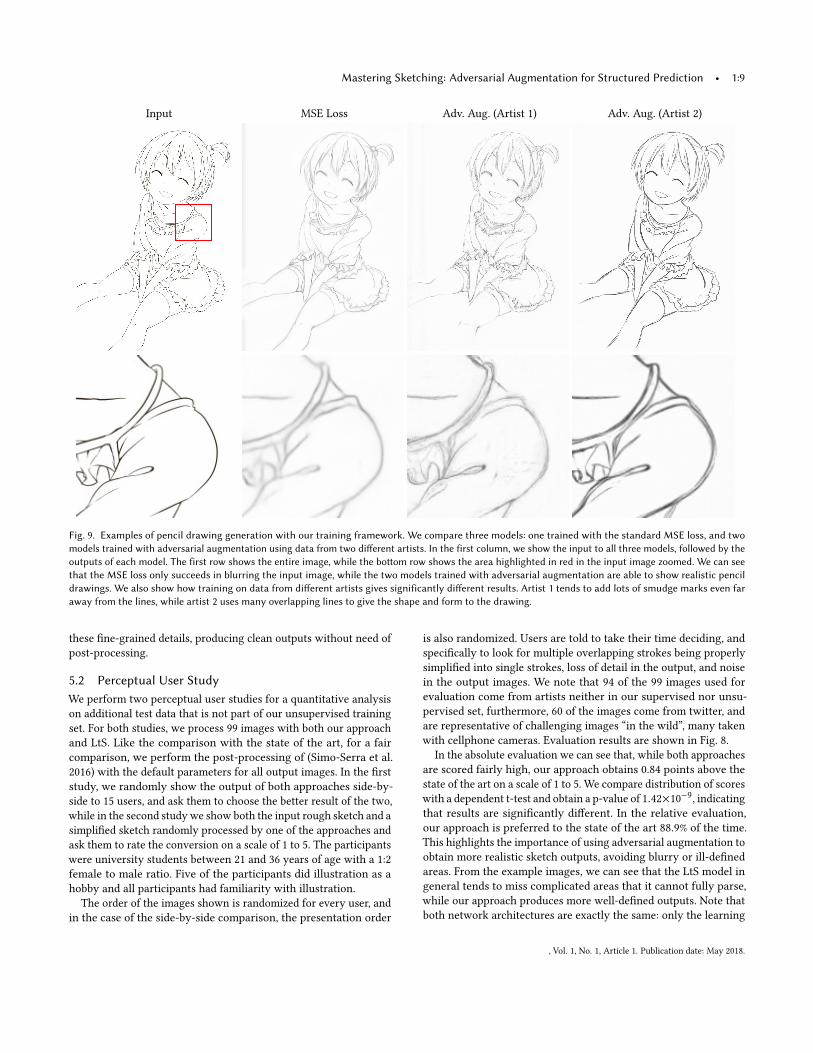
Input MSE Loss Adv. Aug. (Artist 1) Adv. Aug. (Artist 2)

Fig. 9. Examples of pencil drawing generation with our training framework. We compare three models: one trained with the standard MSE loss, and two

models trained with adversarial augmentation using data from two different artists. In the first column, we show the input to all three models, followed by the

outputs of each model. The first row shows the entire image, while the bo�om row shows the area highlighted in red in the input image zoomed. We can see

that the MSE loss only succeeds in blurring the input image, while the two models trained with adversarial augmentation are able to show realistic pencil

drawings. We also show how training on data from different artists gives significantly different results. Artist 1 tends to add lots of smudge marks even far

away from the lines, while artist 2 uses many overlapping lines to give the shape and form to the drawing.

these fine-grained details, producing clean outputs without need of

post-processing.

5.2 Perceptual User Study

We perform two perceptual user studies for a quantitative analysis

on additional test data that is not part of our unsupervised training

set. For both studies, we process 99 images with both our approach

and LtS. Like the comparison with the state of the art, for a fair

comparison, we perform the post-processing of (Simo-Serra et al.

2016) with the default parameters for all output images. In the first

study, we randomly show the output of both approaches side-by-

side to 15 users, and ask them to choose the better result of the two,

while in the second studywe show both the input rough sketch and a

simplified sketch randomly processed by one of the approaches and

ask them to rate the conversion on a scale of 1 to 5. The participants

were university students between 21 and 36 years of age with a 1:2

female to male ratio. Five of the participants did illustration as a

hobby and all participants had familiarity with illustration.

The order of the images shown is randomized for every user, and

in the case of the side-by-side comparison, the presentation order

is also randomized. Users are told to take their time deciding, and

specifically to look for multiple overlapping strokes being properly

simplified into single strokes, loss of detail in the output, and noise

in the output images. We note that 94 of the 99 images used for

evaluation come from artists neither in our supervised nor unsu-

pervised set, furthermore, 60 of the images come from twitter, and

are representative of challenging images “in the wild”, many taken

with cellphone cameras. Evaluation results are shown in Fig. 8.

In the absolute evaluation we can see that, while both approaches

are scored fairly high, our approach obtains 0.84 points above the

state of the art on a scale of 1 to 5. We compare distribution of scores

with a dependent t-test and obtain a p-value of 1.42×10−9, indicating

that results are significantly different. In the relative evaluation,

our approach is preferred to the state of the art 88.9% of the time.

This highlights the importance of using adversarial augmentation to

obtain more realistic sketch outputs, avoiding blurry or ill-defined

areas. From the example images, we can see that the LtS model in

general tends to miss complicated areas that it cannot fully parse,

while our approach produces more well-defined outputs. Note that

both network architectures are exactly the same: only the learning



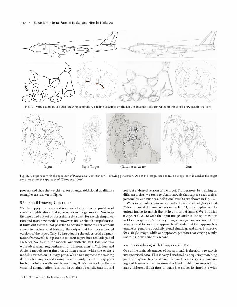
Fig. 10. More examples of pencil drawing generation. The line drawings on the le� are automatically converted to the pencil drawings on the right.

Input Style Target (Gatys et al. 2016) Ours

Fig. 11. Comparison with the approach of (Gatys et al. 2016) for pencil drawing generation. One of the images used to train our approach is used as the target

style image for the approach of (Gatys et al. 2016).

process and thus the weight values change. Additional qualitative

examples are shown in Fig. 6.

5.3 Pencil Drawing Generation

We also apply our proposed approach to the inverse problem of

sketch simplification, that is, pencil drawing generation. We swap

the input and output of the training data used for sketch simplifica-

tion and train new models. However, unlike sketch simplification,

it turns out that it is not possible to obtain realistic results without

supervised adversarial training: the output just becomes a blurred

version of the input. Only by introducing the adversarial augmen-

tation framework is it possible to learn to produce realistic pencil

sketches. We train three models: one with the MSE loss, and two

with adversarial augmentation for different artists. MSE loss and

Artist 1 models are trained on 22 image pairs, while the Artist 2

model is trained on 80 image pairs. We do not augment the training

data with unsupervised examples, as we only have training pairs

for both artists. Results are shown in Fig. 9. We can see how the ad-

versarial augmentation is critical in obtaining realistic outputs and

not just a blurred version of the input. Furthermore, by training on

different artists, we seem to obtain models that capture each artists’

personality and nuances. Additional results are shown in Fig. 10.

We also provide a comparison with the approach of (Gatys et al.

2016) for pencil drawing generation in Fig. 11, which optimizes the

output image to match the style of a target image. We initialize

(Gatys et al. 2016) with the input image, and run the optimization

until convergence. As the style target image, we use one of the

images used to train our approach. We note that this approach is

unable to generate a realistic pencil drawing, and takes 3 minutes

for a single image, while our approach generates convincing results

and runs in well under a second.

5.4 Generalizing with Unsupervised Data

One of the main advantages of our approach is the ability to exploit

unsupervised data. This is very beneficial as acquiring matching

pairs of rough sketches and simplified sketches is very time consum-

ing and laborious. Furthermore, it is hard to obtain examples from

many different illustrators to teach the model to simplify a wide



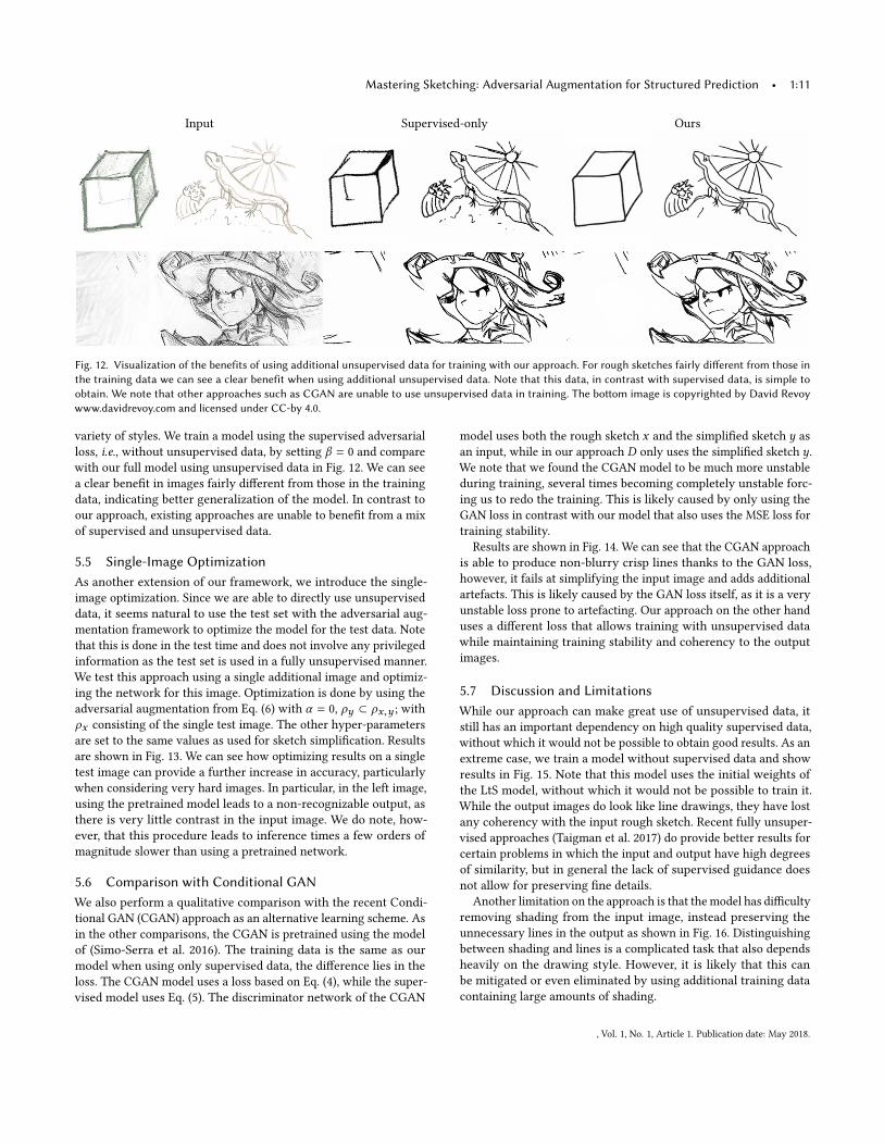
Input Supervised-only Ours

Fig. 12. Visualization of the benefits of using additional unsupervised data for training with our approach. For rough sketches fairly different from those in

the training data we can see a clear benefit when using additional unsupervised data. Note that this data, in contrast with supervised data, is simple to

obtain. We note that other approaches such as CGAN are unable to use unsupervised data in training. The bo�om image is copyrighted by David Revoy


variety of styles. We train a model using the supervised adversarial

loss, i.e., without unsupervised data, by setting β = 0 and compare

with our full model using unsupervised data in Fig. 12. We can see

a clear benefit in images fairly different from those in the training

data, indicating better generalization of the model. In contrast to

our approach, existing approaches are unable to benefit from a mix

of supervised and unsupervised data.

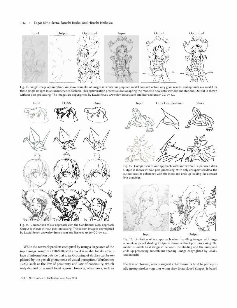
5.5 Single-Image Optimization

As another extension of our framework, we introduce the single-

image optimization. Since we are able to directly use unsupervised

data, it seems natural to use the test set with the adversarial aug-

mentation framework to optimize the model for the test data. Note

that this is done in the test time and does not involve any privileged

information as the test set is used in a fully unsupervised manner.

We test this approach using a single additional image and optimiz-

ing the network for this image. Optimization is done by using the

adversarial augmentation from Eq. (6) with α = 0, ρy ⊂ ρx,y ; with

ρx consisting of the single test image. The other hyper-parameters

are set to the same values as used for sketch simplification. Results

are shown in Fig. 13. We can see how optimizing results on a single

test image can provide a further increase in accuracy, particularly

when considering very hard images. In particular, in the left image,

using the pretrained model leads to a non-recognizable output, as

there is very little contrast in the input image. We do note, how-

ever, that this procedure leads to inference times a few orders of

magnitude slower than using a pretrained network.

5.6 Comparison with Conditional GAN

We also perform a qualitative comparison with the recent Condi-

tional GAN (CGAN) approach as an alternative learning scheme. As

in the other comparisons, the CGAN is pretrained using the model

of (Simo-Serra et al. 2016). The training data is the same as our

model when using only supervised data, the difference lies in the

loss. The CGAN model uses a loss based on Eq. (4), while the super-

vised model uses Eq. (5). The discriminator network of the CGAN

model uses both the rough sketch x and the simplified sketch y as

an input, while in our approach D only uses the simplified sketch y.

We note that we found the CGAN model to be much more unstable

during training, several times becoming completely unstable forc-

ing us to redo the training. This is likely caused by only using the

GAN loss in contrast with our model that also uses the MSE loss for

training stability.

Results are shown in Fig. 14. We can see that the CGAN approach

is able to produce non-blurry crisp lines thanks to the GAN loss,

however, it fails at simplifying the input image and adds additional

artefacts. This is likely caused by the GAN loss itself, as it is a very

unstable loss prone to artefacting. Our approach on the other hand

uses a different loss that allows training with unsupervised data

while maintaining training stability and coherency to the output

images.

5.7 Discussion and Limitations

While our approach can make great use of unsupervised data, it

still has an important dependency on high quality supervised data,

without which it would not be possible to obtain good results. As an

extreme case, we train a model without supervised data and show

results in Fig. 15. Note that this model uses the initial weights of

the LtS model, without which it would not be possible to train it.

While the output images do look like line drawings, they have lost

any coherency with the input rough sketch. Recent fully unsuper-

vised approaches (Taigman et al. 2017) do provide better results for

certain problems in which the input and output have high degrees

of similarity, but in general the lack of supervised guidance does

not allow for preserving fine details.

Another limitation on the approach is that the model has difficulty

removing shading from the input image, instead preserving the

unnecessary lines in the output as shown in Fig. 16. Distinguishing

between shading and lines is a complicated task that also depends

heavily on the drawing style. However, it is likely that this can

be mitigated or even eliminated by using additional training data

containing large amounts of shading.





Input Output Optimized Input Output Optimized

Fig. 13. Single image optimization. We show examples of images in which our proposed model does not obtain very good results, and optimize our model for

these single images in an unsupervised fashion. This optimization process allows adapting the model to new data without annotations. Output is shown

without post-processing. The images are copyrighted by David Revoy www.davidrevoy.com and licensed under CC-by 4.0.

Input CGAN Ours

Fig. 14. Comparison of our approach with the Conditional GAN approach.

Output is shown without post-processing. The bo�om image is copyrighted

by David Revoy www.davidrevoy.com and licensed under CC-by 4.0.

While the network predicts each pixel by using a large area of the

input image, roughly a 200×200 pixel area, it is unable to take advan-

tage of information outside that area. Grouping of strokes can be ex-

plained by the gestalt phenomena of visual perception (Wertheimer

1923), such as the law of proximity and law of continuity, which

only depend on a small local region. However, other laws, such as

Input Only Unsupervised Ours

Fig. 15. Comparison of our approach with and without supervised data.

Output is shown without post-processing. With only unsupervised data, the

output loses its coherency with the input and ends up looking like abstract

line drawings.

Input Output

Fig. 16. Limitation of our approach when handling images with large

amounts of pencil shading. Output is shown without post-processing. The

model is unable to distinguish between the shading and the lines, and

ends up preserving superfluous shading. Image copyrighted by Eisaku

Kubonouchi.

the law of closure, which suggests that humans tend to perceptu-

ally group strokes together when they form closed shapes, is based





on non-local information which can only be approximated with a

fully convolutional network. For large strokes or drawn regions, the

model will be unable to use the full region information and this can

lead to erroneous sketch simplifications of closed regions.

6 CONCLUSIONS

We have presented the adversarial augmentation for structured

prediction and applied it to the sketch simplification task as well

as its inverse problem, i.e., pencil drawing generation. We show

that augmenting the loss of a sketch simplification network with an

adversarial network leads tomore realistic outputs. Furthermore, our

framework allows for unsupervised data augmentation, essential for

structured prediction tasks in which obtaining additional annotated

training data is very costly. As adversarial augmentation only applies

to the training, the resulting models have exactly the same inference

properties as the non-augmented versions. As a further extension

of the problem, we show that the framework can also be used to

optimize for a single input for situations in which accuracy is valued

more than quick computation. This can, for example, be used to

personalize the model to different artists using only unsupervised

rough and clean training data from each particular artist.

REFERENCESSeok-Hyung Bae, Ravin Balakrishnan, and Karan Singh. 2008. ILoveSketch: As-natural-

as-possible Sketching System for Creating 3D Curve Models. In ACM Symposiumon User Interface Software and Technology. 151–160.

Itamar Berger, Ariel Shamir, Moshe Mahler, Elizabeth Carter, and Jessica Hodgins. 2013.Style and abstraction in portrait sketching. ACM Transactions on Graphics 32, 4(2013), 55.

Jiazhou Chen, Gaël Guennebaud, Pascal Barla, and Xavier Granier. 2013. Non-OrientedMLS Gradient Fields. Computer Graphics Forum 32, 8 (2013), 98–109.

Chao Dong, C. C. Loy, Kaiming He, and Xiaoou Tang. 2016. Image Super-ResolutionUsing Deep Convolutional Networks. IEEE Transactions on Pattern Analysis andMachine Intelligence 38, 2 (2016), 295–307.

Alexey Dosovitskiy and Thomas Brox. 2016. Generating Images with PerceptualSimilarity Metrics based on Deep Networks. In Conference on Neural InformationProcessing Systems.

Jean-Dominique Favreau, Florent Lafarge, and Adrien Bousseau. 2016. Fidelity vs.Simplicity: a Global Approach to Line Drawing Vectorization. ACM Transactions onGraphics (Proceedings of SIGGRAPH) 35, 4 (2016).

Jakub Fišer, Paul Asente, Stephen Schiller, and Daniel Sýkora. 2015. ShipShape: A Draw-ing Beautification Assistant. InWorkshop on Sketch-Based Interfaces and Modeling.49–57.

Kunihiko Fukushima. 1988. Neocognitron: A hierarchical neural network capable ofvisual pattern recognition. Neural Networks 1, 2 (1988), 119–130.

Leon A Gatys, Alexander S Ecker, and Matthias Bethge. 2016. Image style transferusing convolutional neural networks. In IEEE Conference on Computer Vision andPattern Recognition.

Ian Goodfellow, Jean Pouget-Abadie, Mehdi Mirza, Bing Xu, DavidWarde-Farley, SherjilOzair, Aaron Courville, and Yoshua Bengio. 2014. Generative adversarial nets. InConference on Neural Information Processing Systems.

Cindy Grimm and Pushkar Joshi. 2012. Just DrawIt: A 3D Sketching System. In nterna-tional Symposium on Sketch-Based Interfaces and Modeling. 121–130.

Xavier Hilaire and Karl Tombre. 2006. Robust and accurate vectorization of linedrawings. IEEE Transactions on Pattern Analysis and Machine Intelligence 28, 6 (2006),890–904.

Takeo Igarashi, Satoshi Matsuoka, Sachiko Kawachiya, and Hidehiko Tanaka. 1997.Interactive Beautification: A Technique for Rapid Geometric Design. In ACM Sym-posium on User Interface Software and Technology. 105–114. http://doi.acm.org/10.1145/263407.263525

Satoshi Iizuka, Edgar Simo-Serra, and Hiroshi Ishikawa. 2016. Let there be Color!: JointEnd-to-end Learning of Global and Local Image Priors for Automatic Image Coloriza-tion with Simultaneous Classification. ACM Transactions on Graphics (Proceedingsof SIGGRAPH) 35, 4 (2016).

Sergey Ioffe and Christian Szegedy. 2015. Batch Normalization: Accelerating DeepNetwork Training by Reducing Internal Covariate Shift. In International Conferenceon Machine Learning.

Phillip Isola, Jun-Yan Zhu, Tinghui Zhou, and Alexei A. Efros. 2017. Image-to-ImageTranslation with Conditional Adversarial Networks. In IEEE Conference on ComputerVision and Pattern Recognition.

Henry Kang, Seungyong Lee, and Charles K. Chui. 2007. Coherent Line Drawing. InInternational Symposium on Non-Photorealistic Animation and Rendering. 43–50.

Yann LeCun, Bernhard Boser, John S Denker, Donnie Henderson, Richard E Howard,Wayne Hubbard, and Lawrence D Jackel. 1989. Backpropagation applied to hand-written zip code recognition. Neural computation 1, 4 (1989), 541–551.

Christian Ledig, Lucas Theis, Ferenc Huszar, Jose Caballero, Andrew P. Aitken, AlykhanTejani, Johannes Totz, Zehan Wang, and Wenzhe Shi. 2017. Photo-Realistic SingleImage Super-Resolution Using a Generative Adversarial Network. (2017).

Chuan Li and Michael Wand. 2016. Precomputed real-time texture synthesis withmarkovian generative adversarial networks. In European Conference on ComputerVision.

David Lindlbauer, Michael Haller, Mark S. Hancock, Stacey D. Scott, and WolfgangStuerzlinger. 2013. Perceptual grouping: selection assistance for digital sketching.In International Conference on Interactive Tabletops and Surfaces. 51–60.

Xueting Liu, Tien-Tsin Wong, and Pheng-Ann Heng. 2015. Closure-aware SketchSimplification. ACM Transactions on Graphics (Proceedings of SIGGRAPH Asia) 34, 6(2015), 168:1–168:10.

Cewu Lu, Li Xu, and Jiaya Jia. 2012. Combining sketch and tone for pencil drawing pro-duction. In International Symposium on Non-Photorealistic Animation and Rendering.65–73.

Mehdi Mirza and Simon Osindero. 2014. Conditional generative adversarial nets. InConference on Neural Image Processing Deep Learning Workshop.

Vinod Nair and Geoffrey E Hinton. 2010. Rectified linear units improve restrictedboltzmann machines. In International Conference on Machine Learning. 807–814.

Hyeonwoo Noh, Seunghoon Hong, and Bohyung Han. 2015. Learning DeconvolutionNetwork for Semantic Segmentation. In International Conference on Computer Vision.

Gioacchino Noris, Alexander Hornung, Robert W. Sumner, Maryann Simmons, andMarkus Gross. 2013. Topology-driven Vectorization of Clean Line Drawings. ACMTransactions on Graphics 32, 1 (2013), 4:1–4:11.

Günay Orbay and Levent Burak Kara. 2011. Beautification of Design Sketches UsingTrainable Stroke Clustering and Curve Fitting. IEEE Transactions on Visualizationand Computer Graphics 17, 5 (2011), 694–708.

Deepak Pathak, Philipp Krähenbühl, Jeff Donahue, Trevor Darrell, and Alexei Efros.2016. Context Encoders: Feature Learning by Inpainting. In IEEE Conference onComputer Vision and Pattern Recognition.

Alec Radford, Luke Metz, and Soumith Chintala. 2016. Unsupervised RepresentationLearning with Deep Convolutional Generative Adversarial Networks. In Interna-tional Conference on Learning Representations.

David E. Rumelhart, Geoffrey E. Hinton, and Ronald J. Williams. 1986. Learningrepresentations by back-propagating errors. In Nature.

Tim Salimans, Ian Goodfellow, Wojciech Zaremba, Vicki Cheung, Alec Radford, andXi Chen. 2016. Improved techniques for training gans. In Conference on NeuralInformation Processing Systems.

Peter Selinger. 2003. Potrace: a polygon-based tracing algorithm. Potrace (online),http://potrace. sourceforge. net/potrace. pdf (2009-07-01) (2003).

Amit Shesh and Baoquan Chen. 2008. Efficient and Dynamic Simplification of LineDrawings. Computer Graphics Forum 27, 2 (2008), 537–545. DOI:https://doi.org/10.1111/j.1467-8659.2008.01151.x

Edgar Simo-Serra, Satoshi Iizuka, Kazuma Sasaki, and Hiroshi Ishikawa. 2016. Learn-ing to Simplify: Fully Convolutional Networks for Rough Sketch Cleanup. ACMTransactions on Graphics (Proceedings of SIGGRAPH) 35, 4 (2016).

Nitish Srivastava, Geoffrey Hinton, Alex Krizhevsky, Ilya Sutskever, and RuslanSalakhutdinov. 2014. Dropout: A Simple Way to Prevent Neural Networks fromOverfitting. Journal of Machine Learning Research 15 (2014), 1929–1958.

Yaniv Taigman, Adam Polyak, and Lior Wolf. 2017. Unsupervised Cross-Domain ImageGeneration. In International Conference on Learning Representations.

Xiaolong Wang and Abhinav Gupta. 2016. Generative Image Modeling using Style andStructure Adversarial Networks. In European Conference on Computer Vision.

Max Wertheimer. 1923. Untersuchungen zur Lehre von der Gestalt, II. PsychologischeForschung 4 (1923), 301–350.

Donggeun Yoo, Namil Kim, Sunggyun Park, Anthony S Paek, and In So Kweon. 2016.Pixel-level domain transfer. In European Conference on Computer Vision.

Matthew D. Zeiler. 2012. ADADELTA: An Adaptive Learning Rate Method. arXivpreprint arXiv:1212.5701 (2012).

Yipin Zhou and Tamara L. Berg. 2016. Learning Temporal Transformations From Time-Lapse Videos. In European Conference on Computer Vision.

Jun-Yan Zhu, Taesung Park, Phillip Isola, and Alexei A Efros. 2017. Unpaired Image-to-Image Translation using Cycle-Consistent Adversarial Networkss. In InternationalConference on Computer Vision.


http://doi.acm.org/10.1145/263407.263525

http://doi.acm.org/10.1145/263407.263525

https://doi.org/10.1111/j.1467-8659.2008.01151.x

https://doi.org/10.1111/j.1467-8659.2008.01151.x

mastering sketching: adversarial augmentation for ...ess/publications/simoserratog2018.pdf ·...

Documents