master’s thesis - connecting repositories · plugging a physical jack into a wall. although the...
TRANSCRIPT

UNIVERSITY OF CYPRUS Computer Science Department
Master’s Thesis
Investigate IPv6 mobility and roaming issues
Christos Charalambous
Supervisor: Associate Professor Andreas Pitsillides
MAY 2007

2
Table of Contents Acknowledgment ...........................................................................................................4 Table of figures ..............................................................................................................6 List of tables...................................................................................................................7 List of Graphs ................................................................................................................8 List of Acronyms ...........................................................................................................9 Abstract ........................................................................................................................11 Chapter 1......................................................................................................................13 Introduction..................................................................................................................13 Chapter 2......................................................................................................................17 Review of literature......................................................................................................17
2.1 Introduction..................................................................................................17 2.2 Mobility – A necessity in today’s networks ................................................17 2.3 Mobile Network Architecture ......................................................................18
2.3.1 Mobile IP Terminology........................................................................18 2.3.2 Mobile IP Functionality .......................................................................19
Mobile IP Overview.........................................................................................19 How Mobile IP Works .....................................................................................20 Agent Discovery ..............................................................................................20 Registration......................................................................................................21 Tunneling .........................................................................................................23
2.4 Mobile Internet Protocol version 6 ..............................................................25 2.4.1 MIPv6 Overview..................................................................................25 2.4.2 MIPv6 Messages & Data Structures ....................................................26
Binding Cache..................................................................................................26 Binding Update List.........................................................................................27 Home Agents List ............................................................................................28
2.4.3 MIPv6 Operation .................................................................................28 Home Agent Registration ................................................................................29 Triangle Routing and Route Optimization.......................................................30 Binding management .......................................................................................32 Movement Detection........................................................................................33 Router Discovery .............................................................................................33 Neighbor Unreachability Detection .................................................................34 Lower Level Indications ..................................................................................34 Evaluations of Movement Detection ...............................................................35 Duplicate Address Discovery ..........................................................................35
2.5 Mobile IPv4 or Mobile IPv6? – Comparison...............................................37 2.6 Mobility and Wireless Local Area Networks (WLANs) .............................39 2.7 Handover......................................................................................................39
Chapter 3......................................................................................................................41

3
Performance Evaluation...............................................................................................41 3.1 Introduction..................................................................................................41 3.2 Problem statement........................................................................................41 3.4 Scenarios ......................................................................................................43
3.4.1 Simulation Scenario 1 ..........................................................................47 3.4.2 Simulation Scenario 2 .........................................................................50 3.4.3 Simulation Scenario 3 .........................................................................52 3.4.4 Simulation Scenario 4 .........................................................................55 3.4.5 Simulation Scenario 5 .........................................................................58 3.4.6 Simulation Scenario 6 .........................................................................61 3.4.7 Simulation Scenario 7 .........................................................................64 3.4.8 Simulation Scenario 8 .........................................................................67 3.4.9 Simulation Scenario 9 .........................................................................69 3.4.10 Simulation Scenario 10 .......................................................................73
Chapter 4......................................................................................................................75 Results and Analysis ....................................................................................................75
4.1 Introduction........................................................................................................75 4.2 Results and Analysis for Scenario 1 ............................................................78 4.3 Results and Analysis for Scenario 2 ............................................................80 4.4 Results and Analysis for Scenario 3 ............................................................83 4.5 Results and Analysis for Scenario 4 ............................................................86 4.6 Results and Analysis for Scenario 5 ............................................................88 4.7 Results and Analysis for Scenario 6 ............................................................91 4.8 Results and Analysis for Scenario 7 ............................................................94 4.9 Results and Analysis for Scenario 8 ............................................................95 4.10 Results and Analysis for Scenario 9 ............................................................96 4.11 Results and Analysis for Scenario 10 ..........................................................98 4.12 Discussion of results and comparison with related work.............................99
Chapter 5....................................................................................................................114 5.1 Conclusion .....................................................................................................114
5.2 Future work................................................................................................116 References - Bibliography .........................................................................................118 APPENDICES ...........................................................................................................122 Appendix 1: Table of scenarios ..............................................................................123 Appendix 2 – Tables of results ..................................................................................128 APPENDIX 3.............................................................................................................147 Supplementary graphs................................................................................................147

4
Acknowledgment I would like to express my sincere gratitude to my supervisor, Associate Professor Andreas Pitsillides. He has offered me great freedom on choosing this topic and developing my interests. He continuously provided me with help and encouragement with extensive knowledge, patient instructions and valuable criticisms. I would also like to thank my family and especially my wife Vaso for her patience until the completion of this thesis. A big thank to my parents and brother for their encouragement and support during my studies.

5
To my daughter and son,
Andreane and Sotiris

6
Table of figures FIGURE 1 PACKET FORWARDING ..........................................................................................................23 FIGURE 2 REVERSE TUNNEL .................................................................................................................24 FIGURE 3 COMPONENTS OF MOBILE IPV6.............................................................................................26 FIGURE 4 MOBILE NODE MOVEMENT ...................................................................................................29 FIGURE 5 HA IS PROVIDED WITH THE NEW COA USING BU AND REPLIES WITH A BACK. ....................30 FIGURE 6 ROUTE OPTIMIZATION ELIMINATES TRIANGLE ROUTING .......................................................31 FIGURE 7 SCENARIO 1...........................................................................................................................47 FIGURE 8 SCENARIO 2...........................................................................................................................50 FIGURE 9 SCENARIO 3...........................................................................................................................52 FIGURE 10 SCENARIO 4 ..........................................................................................................................55 FIGURE 11 SCENARIO 5 ..........................................................................................................................58 FIGURE 12 SCENARIO 6 ..........................................................................................................................61 FIGURE 13 SCENARIO 7 ..........................................................................................................................64 FIGURE 14 SCENARIO 8 ..........................................................................................................................67 FIGURE 15 SCENARIO 9 ..........................................................................................................................69 FIGURE 16 SCENARIO 10 ........................................................................................................................73

7
List of tables TABLE 1 MOBILITY RELATED TERMINOLOGY......................................................................................18 TABLE 2 SCENARIO 1, VIDEO CONFERENCING AND VOICE END-TO-END PACKET DELAY ...................78 TABLE 3 SCENARIO 2, MIPV6 RESULTS ...............................................................................................80 TABLE 4 SCENARIO 2, VIDEO CONFERENCING AND VOICE PACKET END-TO-END DELAY ...................81 TABLE 5 SCENARIO 3, MIPV6 RESULTS ...............................................................................................83 TABLE 6 SCENARIO 3, VIDEO CONFERENCING AND VOICE PACKET END-TO-END DELAY ...................84 TABLE 7 SCENARIO 4, MIPV6 RESULTS ...............................................................................................87 TABLE 8 SCENARIO 4, VIDEO CONFERENCING PACKET END-TO-END DELAY......................................87 TABLE 9 SCENARIO 5, MIPV6 RESULTS ..............................................................................................89 TABLE 10 SCENARIO 5, VIDEO CONFERENCING PACKET END-TO-END DELAY .....................................90 TABLE 11 SCENARIO 6, MIPV6 RESULTS...............................................................................................92 TABLE 12 SCENARIO 6, VIDEO CONFERENCING AND VOICE PACKET END-TO-END DELAY...................93 TABLE 13 SCENARIO 7, MIPV6 RESULTS...............................................................................................94 TABLE 14 SCENARIO 7, CONFERENCING AND VOICE PACKET END-TO-END DELAY..............................94 TABLE 15 SCENARIO 8, MIPV6 RESULTS ..............................................................................................95 TABLE 16 SCENARIO 8, VIDEOCONFERENCING PACKET END-TO-END DELAY.......................................95 TABLE 17 SCENARIO 9, MIPV6 RESULTS ..............................................................................................96 TABLE 18 SCENARIO 9, VIDEO CONFERENCING AND VOICE END-TO-END DELAY ................................97 TABLE 19 SCENARIO 10, MIPV6 RESULTS.............................................................................................98 TABLE 20 VIDEO CONFERENCING PACKET END-TO-END DELAY ..........................................................98 TABLE 21 VALUES OF PARAMETERS TESTED PER SCENARIO ...............................................................123

8
List of Graphs GRAPH 1 VIDEO CONFERENCING AND VOICE END-TO-END DELAY ......................................................79 GRAPH 2 SCENARIO 3, VISITED ACCESS POINTS BY MN_B...................................................................85 GRAPH 3 SCENARIO 3, MN_B TRAFFIC SEND/RECEIVE INTERRUPTION ..................................................86 GRAPH 4 SCENARIO 5, TEST 5.1, HANDOVER PROCESS FOR MN_B.......................................................88 GRAPH 5 TEST 5.3, HANDOVER PROCESS FOR MN_B ............................................................................89 GRAPH 6 TESTS 6.9 AND 6.11 VOICE PACKET END-TO-END DELAY.......................................................91

9
List of Acronyms AP: Access Point.
AR: Access Router.
ARP: Address Resolution Protocol.
BC: Binding Cache.
BR: Binding Request.
BU: Binding Update
BUL: Binding Update List.
CN: Correspondent Node.
CoA: Care-of Address.
DAD: Duplicate Address Detection.
DHCP: Dynamic Host Configuration Protocol.
DHCPv6: Dynamic Host Configuration Protocol version 6.
DNS: Domain Name System.
FA: Foreign Agent.
FBACK: Fast Handover Binding Acknowledgement.
FBU: Fast Handover Binding Update.
GSM: Global System for Mobile Communication.
HA: Home Agents.
HACK: Handover Acknowledgement.
Haddr: Home Address.
HAL: Home Agent List.
HI: Handover Initiation.
HLR: Home Location Register.
HMIPv6: Hierarchical Mobile Internet Protocol version 6.
ICMP: Internet Control Message Protocol.
ICMPv6: Internet Control Message Protocol version 6.
ID: Identification.
IEEE: Institute of Electrical and Electronics Engineers.
IETF: Internet Engineering Task Force.
IP: Internet Protocol.
IPv4: Internet Protocol version 4.
IPv6: Internet Protocol version 6.

10
LAN: Local Area Network.
MAC: Media Access Control.
MIP: Mobile Internet Protocol.
MIPv4: Mobile Internet Protocol version 4.
MIPv6: Mobile Internet Protocol version 6.
MN: Mobile Node.
MTU: Maximum Transmission Unit.
NA: Neighbor Advertisement.
ND: Neighbor Discovery.
NewAR: New Access Router.
NewCoA: New Care-of Address.
NS: Neighbor Solicitation.
NUD: Neighbor Unreachability Detection.
OldAR: Old Access Router.
OldCoA: Old Care-of Address.
PDA: Personal Desktop Assistant.
PrRtAdv: Proxy Router Advertisement.
QoS: Quality of Service.
RA: Router Advertisements.
RCoA: Regional Care-of Address.
RFC: Request For Comments.
RO: Route Optimisation
RS: Router Solicitation.
RtSolPr: Router Solicitation for Proxy.
TCP: Transport Control Protocol.
UDP: User Datagram Protocol.
VC: Video Conferencing
VoIP: Voice Over Internet Protocol
WLAN: Wireless Local Area Network.

11
Abstract Mobility is becoming more and more important in our days mostly because of the
need to support always-on network services like videoconferencing, VoIP etc. In
recent years there is an increase in demand from end-users to access network
resources from anywhere and at any time from all kind of devices. An additional
demand is for the mobile users to receive uninterrupted services.
To overcome the mobility problem, protocols such as MIPv4 (Mobile IPv4) were
designed. Mobile IP offers the ability to users to move (roam) through different
subnetted networks without loosing their connectivity. As the new IPv6 protocol is
emerging and in order to support the IPv6 nodes a new Mobile protocol MIPv6 was
designed. This protocol allows an IPv6 node to be mobile, and arbitrarily change its
location on the IPv6 Internet while still maintain its existing connections.
This thesis investigates IPv6 mobility and roaming issues by simulation. In order to
better understand the MIPV6 protocol it was necessary first to have a good
understanding of the IPv6 protocol in theory and implementation. For that reason the
IPv6 protocol was also implemented on live networks. Furthermore by using the
simulation tool OPNET for different mobility scenarios an attempt was made to
investigate the strengths and weaknesses of the MIPv6 by examining the various
parameters of a MIPv6 environment that could influence the quality of the provided
network services.
In order to investigate mobility and roaming issues in MIPv6 an extensive set of
MIPv6 scenarios were designed and implemented in this thesis. For each scenario
various simulations were run examining different parameters that could influence the
MIPv6 operation and quality of service. The results reveal that MIPv6 can be greatly
influenced from the setting of parameters like Access Point Transmit Power or Mobile
Node Mobility Detection Factor either when these parameters are changed alone or in
combination. This thesis, guided by the results from the simulation scenarios offers
some understanding of the behavior of the MIPv6 protocol, and how the parameters
influence its behavior, and hence their operational setup is discussed.

12
It is worth noting that there is no similar work as in my knowledge where so many
parameters are tested. Some of these parameters are studied in other work but not the
same way as in this thesis. This approach allows one to understand better MIPv6 and
better tune the values of these parameters to a real environment.

13
Chapter 1
Introduction
Internet technology is widespread throughout the world, offering access to varieties of
information and resources. Traditionally, however, the service is only available when
people settle down in their offices, homes or any other authorized areas, typically by
plugging a physical jack into a wall. Although the development of wireless
communication technologies has made wireless Internet access possible, and more
and more portable devices, such as PDAs (Personal Digital Assistants), digital cellular
phones, laptop computers and so on provide Internet access functionality, it does not
mean that Internet communication activities can remain uninterrupted while users are
moving.
Mobile computing and portable computing are two different concepts. If mobile users
only need to be able to launch communication sessions actively before other network
nodes can communicate with them when they are roaming, and do not mind re-
establishing sessions every time they change their access link, portable computing is
sufficient to offer the service. However, mobile computing provides mobile users
anytime, anywhere bidirectional reliable access, and that includes the requirement that
ongoing communication sessions do not need to be restarted even when the point of
attachment to the Internet changes.
Since the Internet Protocol [IP], the core protocol of the Internet, was originally
designed for fixed networks, IP addresses are associated with a fixed network
location, and they are required to remain unchanged during an IP session. Obviously,
this is unable to satisfy the requirements of mobile computing. Therefore, Mobile IP
was proposed by the IETF [Internet Engineering Task Force] in order to offer mobile
users a seamless computing environment.
The basic idea of Mobile IP is to allow a mobile node to have a temporary IP address
in addition to its original fixed IP address. The temporary address is associated with
the current point of attachment to the Internet, while the original fixed IP address

14
represents the location where other network nodes think the mobile node is always
located. This makes it possible that during the movement of the mobile node, its
original fixed IP address remains unchanged, and therefore an ongoing IP session will
not be interrupted.
However, before Mobile IP can be widely deployed, there are still many technical
obstacles, including handover performance, routing efficiency and security issues. As
a result, many Mobile IP supplemental protocols have also been proposed by the IETF
in order to enhance the overall performance and functionality of Mobile IP. It is worth
stating at this point that security issues are out of the scope of this thesis although it is
recognised that security methods can influence the performance of the MIPv6
protocol as well as the general response of the whole mobile environment.
In the OSI [Open System Interconnection] model, Mobile IP can be regarded as a
network layer routing protocol. Due to the fact that mobility performance is the
outcome of the cooperation of different layers, merely focusing on the IP layer
performance is not sufficient. In other words, the Mobile IP operation heavily depends
on lower layer mechanisms, and has direct implications on upper layer performance.
For example, since IP layer communications can only be performed after the link
layer connectivity has been established, the link layer connectivity set-up time directly
affects the Mobile IP signalling latency. Moreover, since Mobile IP affects the routing
path of IP packets, packet losses, delays and reorderings may occur, degrading the
QoS (Quality of Service) and affecting the congestion control mechanism of upper
layers.
To be able to conclude this thesis it was first necessary to have a good understanding
of the internet related technology. A very good knowledge of the IP protocol and its
use in the networks set up was also necessary in order to set-up and implement the
IPv6 environment in live networks. To achieve the previous statement a good
understanding of the IPv6 protocol was necessary. It was also important to study and
understand the features of Mobile IPv6 protocol and how those could be implemented

15
in a network. For that reason a literature review was performed from various
resources including papers, books and articles.
For the simulation part it was necessary to study and learn how to work with the
network software tool OPNET. More specifically the tool was used to simulate all the
scenarios of MIPv6 in a wireless simulated infrastructure while mobile nodes were
using different network applications. For that reason it was also important to have
some knowledge on the Wireless LAN network.
The thesis objective was to investigate the IPv6 mobility and roaming issues by
simulation and understand the behavior of the MIPv6 protocol. Also to examine
different parameters that could influence the MIPv6 operation and quality of service
when the values of these parameters are changed alone or in combination. Finally
propose best parameters values from the results that could be used for MIPv6
optimisation before setting up a MIPv6 environment.
Specifically this thesis is divided into five Chapters and three Appendices,
Chapter 1, is the introduction to the whole thesis where a very brief reference is made
on the thesis subject.
Chapter 2, is the literature review where an elaboration is made on the MIPv6
protocol. An overview of the mobile technology is given and a quick reference is
made on mobility issues.
Chapter 3, discusses performance evaluation in the presence of mobility, where it is
explained what this thesis is using to achieve its objectives. An explanation is given
about the main design issues as well the scenarios and sub-scenarios (named Tests)
that were used for the simulation.
Chapter 4, is the chapter of Results and Analysis, where the findings from the various
scenarios from the previous chapter are presented and analysed. Also, this thesis
results are compared with related work from various papers.
Chapter 5, is the final chapter where some conclusions are formulated and some
further recommendations are made.

16
Appendix 1, tabulates the main MIPv6 parameters that were used for all the simulated
scenarios
Appendix 2, has the tables of MIPv6 results from all the different scenarios
Appendix 3, includes supplementary graphs extracted from the simulated scenarios.

17
Chapter 2
Review of literature
2.1 Introduction
In this chapter a literature review is presented in order to give all the necessary
information needed by the reader to understand the thesis based theory. It starts with a
reference to mobility and continues with explanation of the MIPv6 protocol. It gives a
brief comparison between the protocols MIPv4 & MIPv6 and examines the mobility
issues for the MIPv6 protocol. Since this thesis is using wireless technology to
examine Mobility a quick reference to wireless technology and its features is given.
Also the handover which is a very significant process of mobility is explained.
2.2 Mobility – A necessity in today’s networks
It is a fact that a vast number of electronic devices is in the market that were designed
to offer the best network services to users while traveling. These devices to be able to
offer what they were designed for they need to embed technology that will allow them
to move across the various and different in size networks. A user only cares about the
network services and nothing else. The quality of these services is very important and
any long delays or interruptions are unacceptable. Security is an issue but it is not that
critical for the average user.
Consider the following scenarios,
i. a user travels in his car using his mobile phone. Mobility offers him the ability
to keep talking while moving across the cells and changing mobile base
stations.
ii. a user is walking in a University Campus listening to streaming music using
his PDA which is connected to the wireless network (802.11 protocol).

18
Both scenarios can be made true only because of mobility technology and its features
like roaming and handover. In both cases it would be unacceptable if there was any
kind of interruption or huge delays. To make the above scenarios possible though is
not an easy task. Very well designed networks are needed in order to handle the
continuous movement of a big number of users and of course all these networks have
to communicate with each other with the minimum latency.
It is estimated that in few years the mobile subscribers will be hundreds of millions.
All these users will need to roam through different networks while traveling and of
course receive the same quality of services. It is very important that technology can
support these users and the developing technology is called mobility.
2.3 Mobile Network Architecture
This section explains Mobile IP basic concepts. It applies to either Mobile IPv4 or
Mobile IPv6.
2.3.1 Mobile IP Terminology
The terminology in Table 1 is necessary for the understanding of this thesis.
Mobile Node (MN)
An IP node capable of changing its point of attachment to the network. A Mobile Node may either be a Mobile Host (no forwarding functionality) or a Mobile Router (forwarding functionality).
Correspondent Node (CN)
A peer node with which a mobile node is communicating. The correspondent node may be either mobile or stationary.
Home Agent (HA)
A router on a mobile node's home link with which the mobile node has registered its current care-of address. While the mobile node is away from home, the home agent intercepts packets on the home link destined to the mobile node's home address, encapsulates them, and tunnels them to the mobile node's registered care-of address.
Home Address (HoA)
An IP address assigned to a mobile node, used as the permanent address of the mobile node. This address is within the mobile node's
Table 1 - Mobility Related Terminology

19
home link. Standard IP routing mechanisms will deliver packets destined for a mobile node's home address to its home link
Binding Update (BU)
A message indicating a mobile node's current mobility binding, and in particular its care-of address.
Care-of-Address (CoA)
An IP address associated with a mobile node while visiting a foreign link; the subnet prefix of this IP address is a foreign subnet prefix. A packet addressed to the mobile node which arrives at the mobile node's home network when the mobile node is away from home and has registered a Care-of Address will be forwarded to that address by the Home Agent in the home network.
Foreign subnet prefix
A bit string that consists of some number of initial bits of an IP address which identifies a node's foreign link within the Internet topology.
Home subnet prefix
A bit string that consists of some number of initial bits of an IP address which identifies a node's home link within the Internet topology (i.e., the IP subnet prefix corresponding to the mobile node's home address.
Binding
The association of the home address of a mobile node with a careof address for that mobile node, along with the remaining lifetime of that association.
Registration
The process during which a mobile node sends a Binding Update to its home agent or a correspondent node, causing a binding for the mobile node to be registered.
2.3.2 Mobile IP Functionality
Mobile IP is an open standard, defined by the Internet Engineering Task Force (IETF)
that allows users to keep the same IP address, stay connected, and maintain ongoing
applications while roaming between IP networks. Mobile IP is scalable for the
Internet because it is based on IP meaning any media that can support IP can support
Mobile IP.
Mobile IP provides ubiquitous connectivity for users, whether they are within their
enterprise networks or away from home. Mobile IP is part of both IPv4 and IPv6
standards.
Mobile IP Overview
In IP networks, routing is based on stationary IP addresses. A device on a network is
reachable through normal IP routing by the IP address it is assigned on the network.

20
However, problems occur when a device roams away from its home network and is
no longer reachable using normal IP routing. This causes the active sessions of the
device to be terminated. Mobile IP enables users to keep the same IP address while
travelling to a different network (which may even be operated by a different wireless
operator), thus ensuring that a roaming individual can continue communication
without sessions or connections being dropped.
How Mobile IP Works
The Mobile IP process has three main phases, which are discussed in the following
sections.
• Agent Discovery—A Mobile Node discovers its Foreign and Home Agents
• Registration—The Mobile Node registers its current location with the Foreign
Agent and Home Agent
• Tunneling—A reciprocal tunnel is set up by the Home Agent to the care-of
address (current location of the Mobile Node on the foreign network) to route packets
to the Mobile Node as it roams.
Agent Discovery
During the agent discovery phase, the Home Agent and Foreign Agent advertise their
services on the network by using the ICMP Router Discovery Protocol (IRDP). The
Mobile Node listens to these advertisements to determine if it is connected to its home
network or foreign network.
The IRDP advertisements carry Mobile IP extensions that specify whether an agent is
a Home Agent, Foreign Agent, or both; its care-of address; the types of services it will
provide such as reverse tunneling and generic routing encapsulation (GRE); and the
allowed registration lifetime or roaming period for visiting Mobile Nodes. Rather than
waiting for agent advertisements, a Mobile Node can send out an agent solicitation.

21
This solicitation forces any agents on the link to immediately send an agent
advertisement.
If a Mobile Node determines that it is connected to a foreign network, it acquires a
care-of address. Two types of care-of addresses exist:
• Care-of address acquired from a Foreign Agent - an IP address of a Foreign Agent
that has an interface on the foreign network being visited by a Mobile Node. A
Mobile Node that acquires this type of care-of address can share the address with
other Mobile Nodes.
• Collocated care-of address - an IP address temporarily assigned to the interface of
the Mobile Node itself. A collocated care-of address represents the current position of
the Mobile Node on the foreign network and can be used by only one Mobile Node at
a time.
Registration
When the Mobile Node hears a Foreign Agent advertisement and detects that it has
moved outside of its home network, it begins registration.
The Mobile Node is configured with the IP address and mobility security association
(which includes the shared key) of its Home Agent. In addition, the Mobile Node is
configured with either its home IP address, or another user identifier, such as a
Network Access Identifier.
The Mobile Node uses this information along with the information that it learns from
the Foreign Agent advertisements to form a Mobile IP registration request. It adds the
registration request to its pending list and sends the registration request to its Home
Agent either through the Foreign Agent or directly if it is using a collocated care-of
address and is not required to register through the Foreign Agent. If the registration
request is sent through the Foreign Agent, the Foreign Agent checks the validity of
the registration request, which includes checking that the requested lifetime does not
exceed its limitations, the requested tunnel encapsulation is available, and that reverse
tunnel is supported. If the registration request is valid, the Foreign Agent adds the

22
visiting Mobile Node to its pending list before relaying the request to the Home
Agent. If the registration request is not valid, the Foreign Agent sends a registration
reply with appropriate error code to the Mobile Node.
The Home Agent checks the validity of the registration request, which includes
authentication of the Mobile Node. If the registration request is valid, the Home
Agent creates a mobility binding (an association of the Mobile Node with its care-of
address), a tunnel to the care-of address, and a routing entry for forwarding packets to
the home address through the tunnel.
The Home Agent then sends a registration reply to the Mobile Node through the
Foreign Agent (if the registration request was received via the Foreign Agent) or
directly to the Mobile Node. If the registration request is not valid, the Home Agent
rejects the request by sending a registration reply with an appropriate error code.
The Foreign Agent checks the validity of the registration reply, including ensuring
that an associated registration request exists in its pending list. If the registration reply
is valid, the Foreign Agent adds the Mobile Node to its visitor list, establishes a tunnel
to the Home Agent if reverse tunnel is enabled, and creates a routing entry for
forwarding packets to the home address. It then relays the registration reply to the
Mobile Node.
Finally, the Mobile Node checks the validity of the registration reply, which includes
ensuring an associated request is in its pending list as well as proper authentication of
the Home Agent. If the registration reply is not valid, the Mobile Node discards the
reply. If a valid registration reply specifies that the registration is accepted, the Mobile
Node is confirmed that the mobility agents are aware of its roaming. In the collocated
care-of address case, it adds a tunnel to the Home Agent. Subsequently, it sends all
packets to the Foreign Agent.
The Mobile Node reregisters before its registration lifetime expires. The Home Agent
and Foreign Agent update their mobility binding and visitor entry, respectively,
during reregistration. In the case where the registration is denied, the Mobile Node
makes the necessary adjustments and attempts to register again. For example, if the
registration is denied because of time mismatch and the Home Agent sends back its

23
time stamp for synchronization, the Mobile Node adjusts the time stamp in future
registration requests.
Thus, a successful Mobile IP registration sets up the routing mechanism for
transporting packets to and from the Mobile Node as it roams.
Tunneling
The Mobile Node sends packets using its home IP address, effectively maintaining the
appearance that it is always on its home network. Even while the Mobile Node is
roaming on foreign networks, its movements are transparent to correspondent nodes.
Data packets addressed to the Mobile Node are routed to its home network, where the
Home Agent now intercepts and tunnels them to the care-of address toward the
Mobile Node. Tunneling has two primary functions: encapsulation of the data packet
to reach the tunnel endpoint, and decapsulation when the packet is delivered at that
endpoint. The default tunnel mode is IP Encapsulation within IP Encapsulation.
Optionally, GRE and minimal encapsulation within IP may be used. Typically, the
Mobile Node sends packets to the Foreign Agent, which routes them to their final
destination, the Correspondent Node (Figure 1).
Internet
Home Agent
Correspondent Node
Mobile Node
Foreign Agent
Figure 1 – Packet Forwarding

24
However, this data path is topologically incorrect because it does not reflect the true
IP network source for the data—rather, it reflects the home network of the Mobile
Node. Because the packets show the home network as their source inside a foreign
network, an access control list on routers in the network called ingress filtering drops
the packets instead of forwarding them. A feature called reverse tunnelling solves this
problem by having the Foreign Agent tunnel packets back to the Home Agent when it
receives them from the Mobile Node (Figure 2).
Tunnel MTU discovery is a mechanism for a tunnel encapsulator such as the Home
Agent to participate in path MTU discovery to avoid any packet fragmentation in the
routing path between a Correspondent Node and Mobile Node. For packets destined
to the Mobile Node, the Home Agent maintains the MTU of the tunnel to the care-of
address and informs the Correspondent Node of the reduced packet size. This
improves routing efficiency by avoiding fragmentation and reassembly at the tunnel
endpoints to ensure that packets reach the Mobile Node.
Figure 2 – Reverse Tunnel

25
2.4 Mobile Internet Protocol version 6
2.4.1 MIPv6 Overview
Mobile Internet Protocol version 6 (MIPv6) is a new protocol that allows IPv6 nodes
to be mobile, to arbitrarily change their location on an IPv6 network and remain
reachable. Mobile IPv6 defines a new Mobility header, new mobility messages, new
ICMPv6 messages, and new and updated options to perform mobility functions and
processes. Mobile IPv6 defines the processes and message exchanges for mobile
nodes, home agents, and correspondent nodes when a mobile node changes its
location from its home link to a foreign link, to another foreign link, and returns
home.
When an IPv6 node changes its location, it might also change its link. When an IPv6
node changes its link, its IPv6 address might also change in order to maintain
connectivity. There are mechanisms to allow for the change in addresses when
moving to a different link, such as stateful and stateless address autoconfiguration
[30] for IPv6. These mechanisms are completely transparent for all layers above IP,
e.g. for TCP [9], UDP and of course for all applications. Therefore DNS entries for a
mobile node refer to its home address and don’t change if the mobile node changes its
Internet access point. In fact IPv6 influences the routing of packets but it is
independent of the routing protocol itself i.e RIP, OSPF. The solution given by
MIPv6 consists of creating a so-called care-of-address whenever a node changes its
point of attachment to the web. Figure 3 – Components of Mobile IPv6[24] shows the
MIPv6 Components.

26
2.4.2 MIPv6 Messages & Data Structures
The following data structures are needed to facilitate the processes of Mobile IPv6:
• Binding cache
• Binding update list
• Home agents list
Binding Cache
The binding cache is a table maintained by each correspondent node and home agent
that contains the current bindings for mobile nodes. Each binding cache entry contains
the following information:
• The home address for the mobile node
• The care-of address for the mobile node
• The lifetime of the binding cache entry
Figure 3 – Components of Mobile IPv6

27
The lifetime is obtained from a Lifetime field of the last Binding Update [16] message
that was received for this cache entry.
The information in the binding cache takes precedence over the information in the
neighbour cache. For mobile destinations that are away from home, packets should be
sent to the mobile node's home address by way of its care-of address. If packets are
sent directly to the home address while the mobile node is away from home, the home
agent must intercept the packets and tunnel them to the mobile node, lowering the
efficiency and performance of the communication between the correspondent node
and the mobile node.
Binding Update List
The binding update list is maintained by a mobile node to record the most recent
binding updates sent for the home agent and correspondent nodes. A binding update
list entry contains:
• The address of the node to which the binding update was sent
• The home address for the binding update
• The care-of address sent in the last binding update
• The value of the Lifetime field in the binding update
• The remaining lifetime of the binding
The initial value is the value of the Lifetime field in the binding update. When the
lifetime expires, the entry is deleted from the binding update list.
• The maximum value of the Sequence Number field sent in previous binding updates
• The time that the last binding update was sent
• An indication of whether a retransmission is needed for binding updates sent and
when the retransmission is to be sent
• A flag indicating that no future binding updates need to be sent

28
Home Agents List
Home agents maintain the home agents list and record information about each router
from which a Router Advertisement message was received on the home link. Home
agents maintain the home agents list so that they can send the list of home agents to a
requesting mobile node away from home during home agent address discovery. A
home agent’s list entry contains the following:
• The link-local address of the router on the link, obtained from the source address of
the received Router Advertisement message
• The global address or addresses of the home agent, obtained from the Prefix field in
the Prefix Information options in the Router Advertisement message
• The remaining lifetime of this entry
The initial lifetime is obtained from either the Home Agent Lifetime field in the
Home Agent Information option or the Router Lifetime field in the Router
Advertisement message. When the lifetime expires, the entry is deleted from the home
agents list.
• The preference for the home agent, obtained from the Home Agent Preference field in
the Home Agent Information option
When the mobile node receives the list of home agents, it chooses the first home agent
in the list.
2.4.3 MIPv6 Operation
The Figure 4 shows a MN moving from its home network to a foreign link. The
procedures that will be described in this scenario are Home Agent Registration,
Triangle Routing, Route Optimization and Home Agent Discovery.

29
While the MN resides on the home network, the correspondent nodes use its regular
home address and no CoA is needed.
Home Agent Registration
Figure 5 illustrates when the MN has moved from its home link to link A. Every
router in an IPv6 network sends RA to the all-nodes multicast address periodically.
The MN needs an RA in order to detect movement and add a new default router. The
RA provides the MN with the correct network prefix so that it can start the address
configuration procedure. If the delay between each RA is too long, the MN can
request it by sending a RS. The RA message on this link specifies the prefix, and the
default router will be router A.
Once the RA is received, the MN starts DAD [14] to guarantee the uniqueness of the
generated address by sending a NS. If this procedure is successful, the MN has an
address ready for use on the new link. This new address is referred to as the MNs
CoA. When the MN has acquired its new CoA, the binding update procedures can
begin by sending an IPv6 destination option packet with a BU to the HA. When the
HA receives the BU it registers the new CoA and returns a BACK to the MN
confirming that the binding is accepted. The MN also sends BUs to the nodes listed in
Figure 4 – Mobile Node Movement

30
its BUL. Authentication Header or Encapsulated Security Payload to avoid misuse by
other nodes must protect these binding messages.
InternetHome Link
Link B
Correspondent Node
Mobile Node
Router HRouter B
Router A Link A
Home Agent
Router Advertisment
Binding Update
Binding Acknowledgement
Triangle Routing and Route Optimization
When the MN has received its new CoA, the HA will intercept all packets addressed
to the MNs home address. When the MN sends packets, it sets its CoA as the source
address and includes a home address destination option. A MN is statically configured
with a home address, opposed to the CoA that changes when moving between the
network segments. Protocol layers above IP do not, however, see the changing CoAs
– only the home address. The MN itself sends packets directly to the nodes it
communicates with, known as correspondent nodes (CN). This scenario is known as
triangle routing. The problem with this is that packets may need to traverse a longer
path than necessary, thus causing longer delays. Consider a CN on the same subnet as
the MN far away from the MN’s HA. All packets from the CN must traverse through
the HA although the MN and the CN resides on the same subnet.
A solution to triangle routing is Route Optimization. This provides means for nodes to
cache the binding of a mobile node and tunnel their datagrams directly to its CoA.
Route Optimization is illustrated in Figure 6. The MN has a CoA that is unknown for
Figure 5– HA is provided with the new CoA using BU and replies with a BACK.

31
the CN. The CN delivers the packet to the MN’s home address. The HA intercepts
this packet and tunnels it on to the MN.
When the MN receives the tunneled packet, it is able to detect that this packet is
originating from the CN, thus sending a BU to that address. The CN will register the
new binding in its BC. The next packet addressed to the MN can then be sent directly,
thus avoiding triangle routing.
InternetHome Link
Link B
Correspondent Node
Mobile Node
Router HRouter B
Router A Link A
Home Agent
Router Advertisment
First Packet
Binding update
Second Packet
The BU sent to the MN can decide whether or not the receiver should generate a
BACK. If it chooses to disable BACK, it will know if the binding was received by
inspecting the next packet from this specific node. If that packet comes from the HA,
the binding was not received and the MN should generate a new BU message.
Each binding in the BC is associated with a lifetime. There are two possibilities to
renew the binding when the lifetime expires. The MN can send a new BU, or the CN
can request a new binding by sending a BR.
Figure 6 – Route Optimization eliminates triangle routing

32
Binding management
A mobile node, which configured a new care-of address as primary care-of address,
has to register this new address as its home agent and at the corresponding nodes,
which have been already informed about the mobile node’s binding. For this purpose
the mobile node sends a Binding Update containing its new binding. To make sure
that the intended receiver receives the Binding Update, the mobile node can enforce
the receiver to acknowledge the receipt of the Binding Update by responding with a
Binding Acknowledgement. To trigger this acknowledgement, the mobile node sets
the acknowledgement bit in the Binding Update. Until receipt of the
acknowledgement the mobile node continues retransmitting the Binding Update
periodically.
In case a mobile node receives a packet from a correspondent node it is able to detect,
if the sending correspondent node has already a Binding Cache entry. If the
correspondent node has a Binding Cache entry for that mobile node, it addresses the
packet directly to the mobile node’s care-of address. Otherwise the correspondent
node sends that packet to the mobile node’s home address. In this case the mobile
node receives a tunneled packet. The mobile node may send a Binding Update to the
correspondent node to enable it, to send future packets directly to the mobile node
without tunneling by the home agent.
A mobile node must set the Acknowledgement bit in Binding Updates addressed to a
home agent. The mobile node may also set the Acknowledgement bit in Binding
Updates sent to a corresponding node. If the Binding Update was not received by the
corresponding node, the mobile node would recognize this in receiving still tunneled
packets from the home agent.
Before expiration of a Binding Cache entry for a mobile node the correspondent node
can initiate a refreshing of the binding by sending a Binding Request towards the
mobile node. Receiving this Binding Request the mobile node may reply with a
Binding Update.

33
Movement Detection
An important aspect when considering mobility in IPv6 is how the MNs detect that
they have moved from one link to another. This is critical in order to provide
mobility, since delays in movement detection mechanisms will cause delays in
obtaining a new CoA. This will again decrease the performance when moving
between different networks. The specification of MIPv6 defines that a MN can use
any combination of the mechanisms available to detect that it has moved from one
network to another. These are router discovery, neighbor unreachability detection
(NUD) and indications from the link-layer.
Router Discovery
When a MN moves between networks it can detect routers by waiting for the periodic
router advertisement or it can send a router solicitation. The neighbor discovery
protocol has limits for how often a MN can send solicitations, and these limitations
can prevent the MN to receive router advertisements quickly, thus delaying the
detection of a new router. Therefore, MIPv6 does not impose these strict limitations,
meaning that a MN when away from home can send router solicitations more
frequently. In addition, the interval between router advertisements can be reduced.
This can lead to a reduced overall network performance due to the increased network
traffic, but it will also increase handover performance for the MN. It is important to
remember that the MNs will reside on wireless links with limited bandwidth,
implying that the router solicitation interval will represent a compromise between
handover performance and network load.
The main goal with movement detection mechanisms is that MNs should detect their
new routers as quickly as possible and this implies that there is a balance between
handover performance and the network load created. When considering solicitations,
a maximum number that can be sent has been defined to prevent unnecessary network
load. The only exception is MNs that are moving to another network. They can
exceed this limit if they are currently without a CoA on their new link, thus helping
the MNs to detect a new router more quickly.
There is however a problem with this approach. If a MN increases the RS rate without
knowing that it has moved to a new link, this will cause extra traffic on the old link,
where the MN already is registered with an existing CoA. To prevent this, the MN

34
must know for sure that it has moved to a new link, e.g. by receiving a positive
indication from lower protocol layers (see below). It is also important that MNs
reduces their RS rate after they have received a CoA, to prevent unnecessary network
load.
Neighbor Unreachability Detection
While a MN is away from home and is using some router as default, it is important for
the MN to be able to quickly detect when that router becomes unreachable so that it
can switch to a new default router and to a new care-of address. Since some links (e.g.
wireless) do not necessarily work equally well in both directions, it is likewise
important for the MN to detect when it becomes unreachable for packets sent from its
default router. The MN can then take necessary precautions to ensure that any CN
attempting to communicate with it can still reach it through some other route. This
can be done through the NUD procedure, which is a movement detection mechanism
that can tell the MN if it has moved to a new link.
It is, however, important to remember that the MN cannot efficiently rely on NUD
alone. This is because the network load would be prohibitively high in many cases for
a MN to continually probe its default router with NS messages even when it is not
otherwise actively sending packets to it. To prevent this from happening it is
recommended that the MN can use every received packet from its router as an
indication that it is still reachable on its current care-of address. The router should
send RA messages periodically and the MN will have frequent opportunity to check if
the default router is reachable.
Lower Level Indications
Another possibility for movement detection is obtaining some type of indication about
link-layer mobility from lower protocol layers, or device driver software, controlling
the network interface on the MN. This is especially important when considering
wireless access technologies such as WLAN. A MN can for instance use signal
strength or signal quality information for its link with the available routers to decide
when to switch to a new primary care-of address that could provide a better
connection. It is, however, essential that the MN does not assume that all link-layer
mobility indications from lower levels necessarily means a movement to a new
network segment. Movement from one WLAN cell to another can be made

35
transparent to the IP layer if all the WLAN access points are operating within the
same network segment.
Evaluations of Movement Detection
Movement detection is essential in order to provide mobility in IPv6. Although the
default procedure for this is router discovery, it would be preferable to provide
additional mechanisms in order to prevent too much network load. The NUD can help
the MNs in determining that their default routers are no longer available, thus
indicating that they must change to another care-of address. NUD can also help to
decide whether a MN can increase their RS rate or not, based on advertisements and
indications that the MN really has moved to a new link. The efficiency of movement
detection can also be increased if the MN could obtain indications about link layer
mobility from lower protocol layers. This means that the MN can detect new routers
while still receiving advertisements from its current default router and decide whether
or not to switch based on for instance signal strength in a wireless access technology.
The conclusion is that a MN should use any information possible in order to perform
handover to another network, thus minimizing the delay when changing its primary
care-of address.
Duplicate Address Discovery
A node must perform DAD (Duplicate Address Detection) when it boots up onto an
IPv6 network to ensure that its configured addresses are likely to be unique on the
link, a MN that moves onto a new network must perform DAD on the CoA that it
obtains from the CoA configuration phase. This holds true regardless of whether the
CoA address has been obtained by stateless, stateful or manual means.
In IPv6, the DAD procedure is defined in RFC 2462 “IPv6 Stateless Address
Autoconfiguration”, [47] and uses the neighbour discovery procedures defined in
RFC 2461. A MN cannot begin to use a new CoA until the DAD procedure has been
successfully executed. Until DAD has succeeded, the MN’s new CoA is seen as
tentative, in that it can only be used for neighbour discovery purposes (of which the
DAD procedure is part of). If a MN was to use its new CoA before successful DAD

36
and another node was using the same address on the link, the MN would erroneously
process packets intended for the other node.
To perform DAD, the MN sends out a neighbour solicitation message with its own
new CoA address as the target address of the solicitation message. The destination
address in the IPv6 header of the neighbour solicitation is set to the solicited-node
multicast address of the target address with the source address being the unspecified
address. If there is another node on the link that is using the same address as the MN’s
new CoA, one of two things will happen:
1. The duplicate node will receive the MN’s neighbour solicitation message and reply
with a neighbour advertisement (sent to the all-nodes multicast address) thus exposing
the duplicated address to the MN.
2. The MN will receive a neighbour solicitation with its new CoA as the target
address from a duplicate node that is also in the process of performing DAD.
Thus, the DAD procedure will give an explicit indication to the MN should there be
another node on the network that is using its new CoA. However, (and to the
detriment of any node wishing to perform autoconfiguration at haste) the DAD
procedure provides no explicit indication that a MN’s new CoA is not being used by
another node on the network. Indeed, the point at which DAD can be considered to
have succeeded is quite vague. According to RFC 2462 a node performing DAD
under default conditions will take a minimum of 1 second plus additional delay for
link transmissions and logic computation.
Note that in order to speed up the autoconfiguration process, a MN may choose to
initiate DAD in parallel to router discovery. Since the value of the node’s link-layer
identifier is known in advance, the MN can perform DAD on its link local address
before receiving a router advertisement. If the router advertisement instructs the node
to use stateless address configuration, the MN need not perform DAD on its resultant
global unicast address if it has already verified the uniqueness of it’s link-local
address.

37
As a router may delay responding to a router solicitation by a few seconds, a MN that
performs DAD only after receiving a valid router advertisement may experience
significantly longer autoconfiguration latency than performing the steps in parallel
when stateless addressing is used. However, as noted above, a MN may only detect
that it has moved onto a new network as a result of receiving a new router
advertisement; in which case the potential speed up of performing DAD in parallel to
router discovery is lost.
2.5 Mobile IPv4 or Mobile IPv6? – Comparison
As the new protocol is evolving it is a matter of time for the networks to support it.
Nevertheless a network to support MIPv6 needs to be configured for IPv6. A question
that needs to be answered is what are the benefits to move from IPv4 to IPv6 and
respectively the same for moving from MIPv4 [43] to MIPv6 [42] .
This section provides an overview of the features that differ between Mobile IPv4 and
Mobile IPv6. Mobile IPv6 shares many features with Mobile IPv4, but the protocol is
now fully integrated into IP and provides many improvements over Mobile IPv4.
This section summarizes the major differences between Mobile IPv4 and Mobile
IPv6:
• Due to the shortage of IPv4 addresses there might be problems in assigning IPs for
all mobile nodes. MIPv6 won’t have that problem since the number of IPv6
addresses space is huge.
• Avoid waste of bandwidth. Support for what is known in Mobile IPv4 as "Route
Optimization" is now built in as a fundamental part of the protocol, rather than
being added on as an optional set of extensions that may not be supported by all
nodes as in Mobile IPv4.
• The use of the care-of address as the Source Address in each packet's IP header
also simplifies routing of multicast packets sent by a mobile node. With Mobile
IPv4, the mobile node had to tunnel multicast packets to its home agent in order to
transparently use its home address as the source of the multicast packets [5]. With
Mobile IPv6, the use of the Home Address option allows the home address to be

38
used but still be compatible with multicast routing that is based in part on the
packet's Source Address.
• There is no longer any need to deploy special routers as "foreign agents" as are
used in Mobile IPv4. In Mobile IPv6, mobile nodes make use of IPv6 features,
such as Neighbor Discovery and Address Autoconfiguration, to operate in any
location away from home without any special support required from its local
router.
• Unlike Mobile IPv4, Mobile IPv6 utilizes IP Security for all security requirements
for Binding Updates [27].
• The movement detection mechanism in Mobile IPv6 provides bi-directional
confirmation of a mobile node's ability to communicate with its default router in
its current location (packets that the router sends are reaching the mobile node,
and packets that the mobile node sends are reaching the router).
• Most packets sent to a mobile node while away from home in Mobile IPv6 are
sent using an IPv6 Routing header rather than IP encapsulation, whereas Mobile
IPv4 must use encapsulation for all packets. The use of a Routing header requires
less additional header bytes to be added to the packet, reducing the overhead of
Mobile IP packet delivery [3].
• While a mobile node is away from home, its home agent intercepts any packets
for the mobile node that arrive at the home network, using IPv6 Neighbor
Discovery rather than ARP as is used in Mobile IPv4. The use of Neighbor
Discovery improves the robustness of the protocol and simplifies implementation
of Mobile IP due to the ability to not be concerned with any particular link layer
as is required in ARP.
• The dynamic home agent address discovery mechanism in Mobile IPv6 uses IPv6
anycast and returns a single reply to the mobile node, rather than the
corresponding Mobile IPv4 mechanism that used IPv4 directed broadcast and
returned a separate reply from each home agent on the mobile node's home link.
The Mobile IPv6 mechanism is more efficient and more reliable, since only one
packet need be sent back to the mobile node.

39
• The use of IPv6 destination options allows all Mobile IPv6 control traffic to be
piggybacked on any existing IPv6 packets, whereas in Mobile IPv4 and its Route
Optimization extensions, separate UDP packets were required for each control
message.
• Mobile IPv4 uses UDP for signaling, whereas Mobile IPv6 uses IPv6 extension
headers. This allows for a cleaner implementation, since the code can fully
integrated with the IP-processing where it belongs, and no transport protocol port
numbers need to be bound for special use.
2.6 Mobility and Wireless Local Area Networks (WLANs)
Having in mind that mobility is the movement of the users it means there is a media to
support this movement apart from the mobile protocol. That media can be fixed media
like cabling or the most common used media is the wireless infrastructure. For the
needs of this thesis the media used was the wireless technology.
Although wireless technology is not the most secure communication method since
“all information is in the air”, it is the most practical. Users traveling with vehicles are
changing networks subnets rabidly and the wireless LAN technology offers the best
media to support that movement. Wireless technology is mostly known as Wi-Fi
(Wireless Fidelity) and the supported protocol is the standard 802.11 [10]. A typical
WLAN contains at least one Access Point and on or more clients. An access point can
be integrated to a wireless router which also includes an Ethernet switch, and internal
Router firmware application that provides IP Routing, NAT, and DNS forwarding
through an integrated Wide Area Network (WAN) interface. A wireless router allows
all three devices (mainly the access point and router) to be configured through one
central utility. In this thesis the wireless routers were used during the simulation.
2.7 Handover
As explained earlier a very important process during roaming is the handover.
Handover (or handoff) refers to the event when an MN changes its point of

40
attachment from one access network to another. Handovers is said to be seamless if
the handover is transparent to the user of the MN. Handovers can be categorized as a
hard or soft handover [RFC2461] [46] . In hard handover the terminal has connectivity
to a single access point, either the old or the new one in any point of time. Typically,
wireless technologies, such as IEEE 802.11 employ hard handover. The control of
hard handover is simpler since there is no ambiguity over which access point the
mobile terminal shall communicate. In soft handover the terminal has connectivity to
more than one access point simultaneously. It requires that wireless cells overlap.
Also handover is distinguished in horizontal and vertical [22] [17].
The performance metric of handover is the handover latency which is the time where
the mobile host experiences certain duration without being able to send and receive
data packets. It is commonly described as the time it takes a mobile host to resume
data traffic after the handover event has occurred.

41
Chapter 3
Performance Evaluation
3.1 Introduction
As stated earlier during this thesis OPNET simulator tool was used to investigate
mobility and roaming issues in mobile IPv6. In this chapter the basic scenarios which
were designed are described as well as all the different sub-scenarios (named tests)
that were used to extract the various results. The expected results from each scenario
are described in this chapter and the actual results are presented and analysis is given
in the next chapter. All the parameters that were tested for each scenario are tabulated
in Table 21 in Appendix 1.
3.2 Problem statement
The main features that are going to be evaluated during the simulation scenarios are
mainly delay, overhead, packet loss and binding update. Although there are other
parameters that can influence mobility like security those are out of the scope of this
thesis.
The network applications that were selected during the various scenarios are
videoconferencing, Voice Over IP (VoIP) and FTP, so as to have a mixture of real
time and elastic applications. The videoconferencing though is the main application
that is used for all the scenarios whereas the FTP and VoIP were used just for
comparison reasons.
The IP assignment to the Mobile Nodes was stateless taking advantage of the IPv6
protocol mechanisms. The stateless auto configuration mechanism is used to

42
configure the MNs with their IPv6 addresses without the need to set up a DHCP
server. All is needed is to configure the IPv6 enable router with the prefix information
for the link to which it is attached.
During simulations the following performance issues were considered:
o Delays: Packet round trip time, End to end delay
o Packet loss
o Bandwidth/Overhead usage (due to triangle)
o Handover latency (the time spent during the handover)
o Layer 2 Handover vs. Layer 3 handover
o The impact of QoS and some applications on roaming services
o Tailoring the MIPv6 protocol to provide adequate QoS without wasting
resources
o Enable and disable cases for route optimization are evaluated
o Binding update issues, early binding updates (binding table)
o Transmission Power. MNs are likely to be battery powered, and minimizing
power consumption is important. Therefore, the number of administrative
messages sent over the link by which a MN is directly attached to the Internet
should be minimized, and the size of these messages should be kept as small
as is reasonably possible.
It is worth noting that there is no similar work as in my knowledge where so many
parameters are tested. Some of these parameters are studied in other work but not the
same way as in this thesis. This approach allows one to understand better MIPv6 and
better tune the values of these parameters to a real environment.
The motivation of choosing the specific parameters was to best tune a MIPv6
environment using wireless technology. It will help in setting up a mIPv6 wireless
LAN in an optimised way.

43
3.4 Scenarios
In this thesis a total of 75 simulated scenarios are designed and run in order to
investigate the setting of the various parameters influencing MIPv6, as discussed
above. Many other scenarios were implemented but are not presented here although
their outcomes were useful and used during the results presentation. For better
reference all the scenarios are tabulated in Table 21 in Appendix 1: Table of scenarios.
All the simulation scenarios were carried out using OPNET tool [34], Version
OPNET 12.0.A PL1 (Build 4162). Similar works working with OPNET can be found
in [20] and [21].
To demonstrate the effects of Mobile IPv6 (MIPv6) mechanisms while two mobile
nodes communicate with each other a MIPv6 environment was set-up. The Mobile
IPv6 network environment is composed of four Wireless Local Area Network
(WLAN) access points (APs) connected through an IP cloud which denotes the
internet (Figure 7 - Scenario 1). All four access points are capable of performing
Layer 2 (L2) switching as well as Layer 3 (L3) routing. The core of the network,
represented by the IP cloud, has a constant latency normally of 0.1 seconds. This
value makes it easier to note the effects of the different MIPv6 mechanisms over the
application delay. The latency variation during simulation is a parameter that is used
to note the effects on MIPv6.
Mobile Node A (MN_A) and Mobile Node B (MN_B) communicate to each other by
running different applications but mostly a very light video application is used (Low
Resolution Video of 128X120 pixels, 9 bits/pixel, 10 frames/sec) as a source of
constant UDP traffic. Mobile Node A is the calling party and Mobile Node B is the
called party.
A total of ten different scenarios have been designed in order to investigate the MIPv6
roaming and mobility issues. Each one scenario out of the ten is further used for
creating other scenarios (sub-scenarios which are named Tests) for examining the
behaviour of the MIPv6 mechanisms. Initially (Scenario 1) the MNs are placed at

44
their corresponding home networks. Then MN_A and MN_B move in fixed or
random trajectories around the four access points which are Home Agent A (HA_A),
Home Agent B (HA_B), Foreign Router 0 (FR_0) and Foreign Router 1 (FR_1). Both
MNs use MIPv6 to roam among the various access points in the network.
Other features and parameters that are used during the scenarios simulation to
investigate mobility and roaming issues are given below:
1. Route optimization enabled /disabled
Route optimization is a process in which the MIPv6 is handling the communication
between the various nodes. It eliminates overheads as well as decrease delays. It is
worth examining this to better understand the effects on the MIPv6 environment and
what is the influence in the various scenarios.
2. Core Network latency
Network Latency is a very important parameter since it creates an important delay in
the transmission of packets. Its value depends on the quality of the network and
always desirable to have as low latency as possible. This thesis investigated the
effects of different values of latency on MIPv6 environment.
3. Beacon Interval
Bacons include the necessary information between the communication of nodes and
access points. Beacon Interval specifies the TBTT (Target Beacon Transmission
Time) in seconds. In other words, the AP will try to transmit Beacon frames with a
period specified by the value of this attribute. The actual time when the Beacon is
transmitted by the AP can be slightly off since it may need to wait for the shared
medium to become available for this transmission. Tuning for the best value of this
parameter will help in minimizing the end to end delay.
4. Wireless LAN data rate

45
The data rate in a WLAN is the actual bandwidth of the media which is the wireless
network. Altering this parameter has direct effect in the communication between the
nodes and access points. Data rate is an essential parameter to tune on access points
while setting up a wireless network so this thesis investigates the best tuned value.
5. Mobile Node velocity
Velocity is an important parameter which it is believed to influence the MIPv6
environment. This thesis investigated a node while changing its ground speed and
examines the effects on MIPv6 environment. This parameter is worth going under test
since mobility has the meaning of moving IP devices and it worth examining the
effects of the velocity on the MIPv6 environment.
6. Access Point transmit power
Although changing transmit power of a device like access point or mobile node has
other effects on the device ie on battery life, it is an important parameter to be tested
since altering the access point transmit power has direct effects on handover process.
7. TCP Buffer size
This is the size of the buffer holding received data before it is forwarded to the higher
layers (e.g. applications). In this thesis the size of this buffer is examined to
investigate the effects of its alteration on the MIPv6 environment.
8. Mobility Detection Factor
Mobility Detection Factor, Represents the maximum number of routing
advertisement periods this node will wait without receiving a router advertisement
from its default router, before it consider the default router as not reachable. It is an
important parameter and it worth examining the influence on the MIPv6 environment
while altering its value.
9. Random Roaming
It is true that devices trajectories most of the time are random and not fixed. The
purpose of the examination of this parameter is to compare the results between the
fixed and random trajectories in a simulated environment.

46
10. Network application (VoIP, VC, FTP)
Mobility is necessary for the IP devices to help them maintain the communication
between the network application. Examining some of the most common network
applications like VoIP and Video Conferencing will give good indication how
network applications get influenced in a wireless MIPv6 environment.
11. Binding update interval
Binding update interval is a very important parameter in the MIPv6 technology which
is used to update the MIPv6 devices about the status of the network topology. The
period of this interval is going under test in this thesis to examine the effects on the
MIPv6 results like end to end delay and MIPv6 overheads.
All the above parameters are examined either alone or as a combination during
simulation of the ten scenarios. The specific parameters are part of the various
procedures that take place in the MIPv6 mechanism like handover. Further discussion
on the effect of these parameters on the MIPv6 performance is made in the next
Chapter.
It is worth noting that the method used for simulating the scenarios didn’t follow any
strict rules or any trial and errors effort but it was more something extracted from my
personal experience. The method used was to examine first very simple scenarios
even static environments and end up with a quite complex scenario where both MNs
are moving. This method is helpful to better understand the behaviour of the
parameters under test in the MIPv6 environment.
The simulation times were chosen arbitrarily and didn’t follow any pattern selection.
During the tests where the velocity was under investigation the simulation time was
changing according to velocity increment or decrement.

47
3.4.1 Simulation Scenario 1 – Both Mobile Nodes situated in their Home Agent
Figure 7 shows the position of the MNs in the MIPv6 environment during scenario 1.
Scenario 1 Description:
Scenario number 1 is the basic scenario where both MNs are situated by their HAs.
There is no movement during the simulation and during the alteration of the various
parameters. It is a static environment and it is used to examine the set up without the
MIPv6 mechanisms. Totally five different tests were run for this scenario.
Opnet Models used:
During the scenario 1 the following Opnet models were used,
1. Two Mobile Nodes,
a. MN_A with IPv6 address 2001:193::2
b. MN_B with IPv6 address 2001:192::27
Figure 7 - Scenario 1

48
Each MN is presented by the symbol,
2. Four Access Points with routing capabilities,
a. HA_A with IPv6 address 2001:193::1,
b. HA_B with IPv6 address 2001:192::1,
c. FR_0 with IPv6 address 2001:200::2,
d. FR_1 with IPv6 address 2001:197::1
Each AP is presented by the symbol,
3. Four links with T1 speed each one connecting the four access points with the
internet in a star topology
4. An IP cloud denoting the internet which is represented by the symbol,
.
5. Four coloured ellipse shapes representing the area around the four AP, but
note that it does not represent the exact covered area.
6. An Application Model where the used network applications were configured
and used as a reference for the Profile Model. The Application model is
represented by the symbol,
7. A Profile Model where the network applications that were configured in
Application Model are assigned to a name creating a specific profile. This
profile is then assigned to any Mobile Node. The profile name is presented by
the symbol,

49
Parameters to examine:
In this static environment the parameters that are altered are the ‘Core Network
Latency’ and the network application running on MNs. Three different values of
network latency are examined which are, 0.1, 0.05 and 0.001 seconds. Also the
network applications that were used are Video Conferencing (VC) and Voice Over IP
(VoIP).
Simulations Purpose:
The results after changing the core network latency in this static environment are
expected to have analogous effects on the delay and overall performance on the
network applications. Despite that I believe it is necessary to perform these tests for
future reference and comparison when MIPv6 mechanisms will be examined. It is
expected that as the latency is decreased both delay and overhead will also be
decreased. Packet loss is not expected to be influenced since the environment is not
changing dynamically.
Simulation time:
18 minutes

50
3.4.2 Simulation Scenario 2 – Both MNs situated in the same area of HA_A
The figure 8 shows the position of the MNs in the MIPv6 environment during scenario 2.
Scenario 2 Description:
During scenario number 2 both MNs are situated in the area of HA_A. There is no
movement during the simulation and during the alteration of the various parameters. It
is a static environment and it is used to examine the MIPv6 behaviour the specific
time when a MN is at the corresponding node HA_A. At this scenario MN_B is away
from its HA and MN_A behaves as a Corresponding Node (CN).
Totally six different tests were run for this scenario.
Figure 8 – Scenario 2

51
Opnet Models used:
Scenario 2 uses all the Opnet models as in scenario 1.
Parameters to examine:
In this static environment the parameter that is altered is the ‘Core Network Latency’
in combination with the ‘Route Optimisation’ (RO) feature enabled and RO feature
disabled. Three different values of network latency are defined which are, 0.1, 0.05
and 0.001 seconds. Also during scenario 2 the ‘MN Network Applications’ VC and
VoIP are tested while RO is enabled.
Simulations Purpose:
The MN_B is situated in a CN area and MIPv6 protocol is used. It is expected that
network latency will have the same influence on the overall performance as in
scenario 1. The difference here is that RO disable feature is used which is expected to
increase the overhead and delay during simulation.
Simulation time:
18 minutes

52
3.4.3 Simulation Scenario 3 – MNB movement to FR0
The Figure 9 shows the position of the MNs in the MIPv6 environment during
scenario 3.
Figure 9 – Scenario 3
Scenario 3 Description:
During scenario number 3 MN_A is situated in the area of its Home Agent, HA_A.
For the first time movement of a MN is introduced. The movement is performed by
the MN_B and it can be described as follows:
Movement of MN_B:
(Trajectory 1A) - MN_B moves in a trajectory roaming from HA_B to FR_0 and
returning to HA_B.

53
MN_A is behaving as a CN. In this scenario we can observe that the movement of
MN_B is between two different subnet networks where is necessary to use L3 routing.
MN_B trajectory parameters are as follows,
Traverse time - is the exact time that the MN has travelled for each part of the
trajectory (between the previous and next point).
Ground speed - is the speed (velocity) that the MN is travelling with.
Wait Time - is the time where the MN stops and waits before it starts moving again.
Accumulative time - is the total time that is accumulated form the starting point.
Number 1 is the starting point where MN_B waits for 1 minute before start.
Number 2 is the point where MN_B stops and waits for 2 minutes in the area of FR_0
Number 3 is the returning point for MN_B to its HA (HA_B).
Totally six different tests were run for this scenario.
Opnet Models used:
Further to Opnet models used in Scenario 1, in the Scenario 3 a trajectory model is
introduced. Trajectory is represented by an arrow indicating the direction of the MN’s
movement.
Parameters to examine:
In this mobile environment the parameter that is altered is the core network latency in
combination with the ‘Route Optimisation’ (RO) feature enabled and RO feature
disabled. Two different values of network latency are examined which are, 0.1 and
0.05 seconds. Also apart from VC the VoIP ‘MN Network Application’ is tested for
RO enabled and RO disabled.

54
Simulations Purpose:
MN_B is on the move roaming from its HA to a FR. It is expected that network
latency will have the same influence on the overall performance as in scenario 1 and
2. This scenario is used to examine mobility effect when a MN is moving in a foreign
subnet from its home subnet.
Simulation time:
33 minutes

55
3.4.4 Simulation Scenario 4 – MNB is travelling through IP cloud (Internet)
The Figure 10 shows the position of the MNs in the MIPv6 environment during
scenario 4.
Scenario 4 Description:
During scenario number 4 MN_A is situated in the area of its Home Agent, HA_A.
MN_B is moving through IP cloud (internet). The movement that is performed can be
described as follows:
Figure 10 – Scenario 4

56
Movement of MN_B:
(Trajectory 1A) - MN_B moves in a trajectory roaming from HA_B to HA_A and
returning to HA_B.
MN_A is behaving as a CN. In this scenario we can observe that the movement of
MN_B is between two different subnet networks where is necessary to use L3 routing.
While MN_B is in the area of HA_A then the communication is done using the same
AP which means that is done with L2 switching.
Also MN_B while travelling through internet looses connection with its HA as well as
with its CN which is HA_A and it re-establish connection as soon as it enters the
border of the HA_A covered area.
MN_B trajectory parameters are as follows,
Number 1 is the starting point where MN_B waits for 1 minute before start.
Number 2 is the point where MN_B stops and waits for 2 minutes in the area of
HA_A
Number 3 is the returning point for MN_B to its HA (HA_B).
Totally four different tests were run for this scenario.
Opnet Models used:
As in scenario 3
Parameters to examine:
In scenario 4 the parameter that is altered is the core network latency in combination
with the ‘Route Optimisation’ (RO) feature enabled and RO feature disabled. Two
different values of network latency are examined which are, 0.1 and 0.05 seconds.

57
Simulations Purpose:
MN_B is on the move roaming from its HA to the area of HA_A. It is expected that
network latency will have the same influence on the overall performance as in
scenario 1 to 4. An extra interest here is that the MN_B loses connection and re-
establish connection with its CN (HA_A) which is expected to add some more delay,
overhead and possible increase in the packet loss.
Simulation time:
36 minutes

58
3.4.5 Simulation Scenario 5 – MNB travels to HAA through FR0
The Figure 11 shows the position of the MNs in the MIPv6 environment during
scenario 5.
Figure 11 – Scenario 5
Scenario 5 Description:
During scenario number 5 MN_A is situated in the area of its Home Agent, HA_A.
MN_B is moving towards HA_A through FR_0. The movement that is performed can
be described as follows:
Movement of MN_B:
(Trajectory 1A) - MN_B moves in a trajectory roaming from HA_B to FR_0, then to
HA_A and returning from the same route back to HA_B. MN_A is behaving as a CN.
In this scenario we can observe that the movement of MN_B is between three

59
different subnet networks where is necessary to use L3 routing. Also at the time when
MN_B in the area of HA_A L2 switching is established between MN_A and MN_B.
MN_B trajectory parameters are as follows,
Number 1 is the starting point where MN_B waits for 1 minute in the area of HA_B
before it starts roaming.
Number 2 is the point where MN_B is in the area of FR_0 and turns right towards
HA_A.
Number 3 is the returning point for MN_B from area HA_A back to FR_0.
Number 4 is the point where MN_B is in the area of FR_0 heading towards HA_B.
Number 5 is the point when MN_A returns and stops to HA_B.
Totally four different tests were run for this scenario.
Opnet Models used:
As in scenario 3
Parameters to examine:
In scenario 5 the parameter that are examined are the different APs ‘Data Rate’ and
the APs ‘Transmit Power’. Note that the core network latency in this scenario is kept
constant at 0.1sec and the Route Optimisation (RO) feature is enabled. Two different
values of data rate are examined which are, 1Mbps and 11Mbps. Also the transmit
power of HA_A and FR_0 is altered to 0.05W while data rate is at 1Mbps. The value
of 0.05W is ten times bigger than the default/normal one that is used in the various
scenarios.

60
Simulations Purpose:
MN_B is on the move roaming from its HA to a HA_A. It is expected that data rate
will not have much influence on the packet loss or the delay. The increase of the
transmit power is expected to force for faster handover of the MN_B roaming.
Simulation time:
50 minutes

61
3.4.6 Simulation Scenario 6 – MNB circle movement travelling through the
areas of all routers
The Figure 12 shows the position of the MNs in the MIPv6 environment during
scenario 6.
Figure 12 – Scenario 6
Scenario 6 Description:
During scenario number 6 MN_A is situated in the area of its Home Agent, HA_A.
MN_B is moving through the areas of all access points in a clockwise trajectory. The
movement that is performed can be described as follows:
Movement of MN_B:
(Trajectory 1A) - MN_B moves in a trajectory roaming continuously through areas of
HA_B, FR_0, HA_A, FR_1 and stops at HA_B. MN_A is behaving as a CN. In this
scenario we can observe that the movement of MN_B is between the four different

62
subnet networks where is necessary to use L3 routing. While travelling in the area of
HA_A, L2 switching is established between MN_A and MN_B.
MN_B trajectory parameters are as follows,
i. For the scenario where ground speed is approximately 60-70mph
ii. For the scenario where ground speed is approximately 30mph
iii. For the scenario where ground speed is approximately 120mph
Points 1 to 9 represent each angle of the polygon trajectory and are explained as in
previous scenarios. Totally 11 different tests were run for this scenario.

63
Opnet Models used:
As in scenario 3
Parameters to examine:
In scenario 6 the parameters that are altered are the ‘Beacon Interval’, the ‘Ground
Speed’, the ‘MN Network Application’ and the ‘MN Mobility Detection Factor’.
Some of these parameters are altered in combination. For further details regarding
combinations of the parameters alteration the reader can refer to table Table 21 in
Appendix 1. Note that the core network latency in this scenario is kept constant at
0.1sec and the Route Optimisation (RO) feature is enabled.
Simulations Purpose:
MN_B is on the move roaming from its HA to a HA_A. It is expected that while
beacon interval becomes smaller the delay will be decreased but the overhead should
be increased.
Simulation time:
20 minutes with ground speed is approximately 60-70mph
25 minutes with ground speed is approximately 30mph
19 minutes with ground speed is approximately 120mph

64
3.4.7 Simulation Scenario 7 – MN_A and MN_B travelling to FR1 and FR0
respectively
The Figure 13 shows the position of the MNs in the MIPv6 environment during
scenario 7.
Scenario 7 Description:
During scenario number 7 MN_A is situated in the area of its Home Agent, HA_A
and MN_B in its Home Agent, HA_B. MN_A is moving from HA_B to FR_0 while
at the same time MN_A roams from HA_A to FR_1. The movement that is performed
can be described as follows:
Figure 13 – Scenario 7

65
Movement of MN_A:
(Trajectory 1B)- MN_A moves in a trajectory roaming from HA_A to FR_1 and
returning to HA_A.
Movement of MN_B:
(Trajectory 1A)- MN_B moves in a trajectory roaming from HA_B to FR_0 and
returning to HA_B.
This is the first scenario where both MNs move away from their HA at the same time.
In this scenario we can observe that both MNs are roaming into different subnet
networks.
MN_A trajectory parameters are as follows,
MN_B trajectory parameters are as follows,
Points 1 to 3 represent each point of the trajectory of the movement of the MNs.
Totally four different tests were run for this scenario.
Opnet Models used:
As in scenario 3
Parameters to examine:
In scenario 7 the parameters that are altered are the ‘TCP Buffer Size’ in combination
with the ‘MN Network Application’. TCP Buffer size is changed from 8760 to 32768
for both VC and VoIP Network Applications.

66
Simulations Purpose:
Both MNs move to a different FR area. These tests are examining the effect of TCP
buffer size while both MNs are performing Layer 3 handover while running network
applications.
Simulation time:
32 minutes

67
3.4.8 Simulation Scenario 8 – Both MNs travel to FR_0
The Figure 14 shows the position of the MNs in the MIPv6 environment during
scenario 8.
Scenario 8 Description:
During scenario number 8 MN_A is situated in the area of its Home Agent, HA_A
and roams to FR_0. MN_B is moving from HA_B to FR_0. The movement that is
performed can be described as follows:
Movement of MN_A:
(Trajectory 1B)- MN_A moves in a trajectory roaming from HA_A to FR_0 and
returning to HA_A.
Figure 14 – Scenario 8

68
Movement of MN_B:
(Trajectory 1A)- MN_B moves in a trajectory roaming from HA_B to FR_0 and
returning to HA_B.
In this scenario we can observe that both MNs are roaming into different subnet
networks and meet at FR_0 area.
MN_A trajectory parameters are as follows,
MN_B trajectory parameters are as follows,
Points 1 to 3 represent each point of the trajectory of the movement of the MNs.
Totally four different tests were run for this scenario.
Opnet Models used:
As in scenario 3
Parameters to examine:
In scenario 8 the parameter that is altered is the transmit power of FR_0, HA_A and
HA_B.
Simulations Purpose:
Both MNs roam to area of FR_0 and then return to their HAs. Scenario 8 examines
the effect of transmit power alteration on handover process.
Simulation time:
36 minutes

69
3.4.9 Simulation Scenario 9 – MN_A follows anticlockwise trajectory and
MN_B perform two continues different trajectories
The Figure 15 shows the position of the MNs in the MIPv6 environment during
scenario 9.
Figure 15 – Scenario 9
Scenario 9 Description:
During scenario number 9 both MNs roam away from their HAs performing specific
trajectories and returning after some time back to the initial position. The movement
that is performed can be described as follows:

70
Movement of MN_A:
(Trajectory 1A)- MN_A moves in a counterclockwise trajectory roaming through all
four access points in the network.
Movement of MN_B:
(Trajectory 1B) - MN_B moves, first in a clockwise trajectory roaming through all
four access points in the network.
(Trajectory 2B) - Then it moves counterclockwise re-visiting all access points again.
MN_B trajectory parameters are as follows,
For MN_A when ground speed is approximately 62mph
For MN_B when ground speed is approximately 62mph
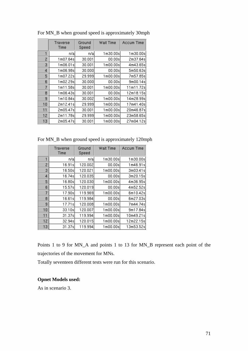
71
For MN_B when ground speed is approximately 30mph
For MN_B when ground speed is approximately 120mph
Points 1 to 9 for MN_A and points 1 to 13 for MN_B represent each point of the
trajectories of the movement for MNs.
Totally seventeen different tests were run for this scenario.
Opnet Models used:
As in scenario 3.

72
Parameters to examine:
In scenario 9 the parameters that are altered are all the parameters that have been
tested in the previous scenarios which are,
o Route optimization enabled
o Route optimization disabled
o Core Network latency
o Beacon Interval
o Wireless LAN data rate
o Mobile Node velocity
o Access Point transmit power
o TCP Buffer size
o MN Mobility Detection Factor
The above parameters are altered and tested either alone or in combination between
them.
Simulations Purpose:
Both MNs are visiting all APs and during their movement they communicate either
establishing L2 or L3 connection. Scenario 9 examines the effect of all parameters
tested in the previous scenario in order to compare the results as well as to find the
best parameters combination for better MIPv6 performance.
Simulation time:
18 minutes when velocity

73
3.4.10 Simulation Scenario 10 – Random Mobility
The Figure 16 shows the position of the MNs in the MIPv6 environment during
scenario 10.
Scenario 10 Description:
Both MNs move randomly in the predefined area. Four different areas were created
named,
- Random_HAA_FR0, where MN_A moves
- Random_HAA_FR1, where MN_A moves
- Random_HAB_FR0, where MN_B moves
- Random_HAB_FR1, where MN_B moves
Figure 16 – Scenario 10

74
Totally six different tests were run for this scenario.
Opnet Models used:
Further to models as in scenario 3 here it is used a model with a name “Mobility
Config” where the mobility domains are specified. A Mobile Node can randomly
move in any point inside the Mobility Domain during the simulation. A mobility
configuration object holds random mobility parameters as profiles, making it easy to
reuse them. The Mobility Config model is represented with the symbol
Parameters to examine:
In scenario 10 the parameter that is tested is the random mobility of both MNs in
combination with the alteration of ‘MN Mobility Factor’, ‘WLAN Data Rate’ and
‘Beacon Interval’.
Simulations Purpose:
Both MNs move in the Mobility Domains as per the various tests. The purpose is to
study the effect of the random roaming and compare the results with the previous
scenarios where the trajectories of the MNs were fixed.
Simulation time:
25 minutes

75
Chapter 4
Results and Analysis
4.1 Introduction
This Chapter presents the results of the ten simulation scenarios from the previous
Chapter. Each scenario results are presented in tables and graphs followed by
analysis.
The results/statistics from the ten scenarios show three main aspects of the dynamics
for the communication between the two MNs which are
• Application traffic,
• Mobile IPv6 measurements and
• Visited access points.
The results can be used to compare the behaviour of MIPv6 environment while
altering the various parameters. All the results that are tabulated in the tables have
been extracted from the OPNET simulation tool output.
It is worth discussing a bit the three main aspects for the two MNs as referred above.
1) Application traffic.
Some gaps in the communication (observe videoconferencing and VoIP traffic
received statistics) can be observed. Each gap is produced every time a mobile
changes its current access point triggering MIPv6 binding procedures to inform its
home agent about its new Care-of Address (CoA). When route optimization is used
the mobile will also inform all its correspondent nodes about its new CoA. While the

76
binding procedure updates home agent and correspondent nodes all traffic directed to
the mobile will be lost.
The application response time will be directly affected by the MIPv6 mechanism used
by the mobile in order to communicate with correspondent nodes. There are two
possible mechanisms used by MIPv6 which are Route Optimization and
Tunnel/reverse tunnel (Route Optimization disabled).
Notice that when RO is enabled the application delay is reduced compared to the case
when route optimization is disabled.
2) Mobile IPv6 measurements
In all scenarios two mobile nodes communicating with each other. This means that at
some point in the simulation the mobile nodes will be acting as both a mobile node
and/or a correspondent node. This cause interesting MIPv6 effects that can be
observed at the "Mobile IPv6 Traffic" statistic tables:
A) When both mobiles are away from their corresponding home networks a
double MIPv6 overhead will occur, either:
• Two MIPv6 tunnels will be needed for the mobiles to communicate. In this
case the application response time delay will be mainly produced by the
three times the data packet must pass through the IP cloud (Internet).
Given the initial latency values for the IP cloud is 0.1 sec, the total
application delay will be approximately 0.3 seconds.
• Two IPv6 extension headers (routing extension header and destination
extension header) will be used (at the same time) to transport the data
traffic when using route optimization mechanism. In this case the
application response time will be mainly produced by only one time the
data packet must pass through the IP cloud (approximately 0.1 sec.). This
is when both mobiles are away from home but located in different
networks. Now, when both mobiles are located at the same access point,
the data packets will just go through the access point, reducing the
application response time even more. For example in scenario 9 in test 9.1

77
this can be observed starting approximately at time 2 min. 20 sec., until
time 8 min. 30 sec.
B) When only one mobile is away from its home network, it will act as a mobile
while the other one will perform correspondent node operations. In this case:
• One MIPv6 tunnel will be needed to communicate.
• Just one MIPv6 extension header (at a given time) will be used to transport
the data traffic when using route optimization mechanism. For example in
scenario 9, test 9.2, an example of this can be observed starting
approximately at time 8 min. 30 sec. until time 16 min. 32 sec.
3) Visited access points
Under this statistic tables it is possible to observe all access points that were visited by
both mobiles. Each bar in the graph represents an access point visited by the mobiles,
and the bar width represents the time the mobile used the access point until it moved
to a different one. The colours of the bars have been set so each one identifies one of
the four access points. By these graphs we can observe the handover times. Measures
are sometimes given as variation which is an instance of change or the rate or
magnitude of change. During this Chapter we note the changes that take place after
the alteration of the various parameters. Further results are tabulated in Appendix 2.

78
4.2 Results and Analysis for Scenario 1
As stated earlier in scenario 1 the only parameter that is changed is the ‘Core Network
Latency’. In simulation applications, 'Core Network Latency' refers to the time delay,
normally measured in milliseconds, between initial input and an output. Latency is
sometimes also called transport delay.
The Table 2 shows the End-to-End Delay in seconds for the two types of Network
Applications that are tested while changing the ‘Core Network Latency’. This delay is
also presented in the Graph 1 below.
Refer to Table 21 for the exact values of the parameters that have been changed
during the Tests.
Statistic Video Conferencing Packet End-to-End
Delay (sec)
Average Maximum Minimum
Test 1.1 0.10677
0.10710 0.10676
Test 1.2 0.056765
0.057083 0.056757
Test 1.3 0.0077702
0.0085166 0.0077570
Test 1.5 0.056766 0.057112 0.056757
Statistic Voice Packet End-to-End Delay (sec)
Test 1.4 0.18341 0.18342 0.18341
Test 1.5 0.13347 0.13348 0.13346
Table 2 – Scenario 1, Video Conferencing and Voice End-to-End Packet Delay

79
As it can be seen from the Graph 1 as the Core Network Delay decreases the Video
Conference and Voice End-to-End Delay also decreases. In both cases as it can be
seen from the tables in Appendix 1 for this scenario when running VoIP there are
almost no packet loss in traffic according to results where traffic received is 2,956.78
and traffic sent 2,956.96 in bytes/sec. Also the same stands for VC where traffic sent
is 324.95 and traffic received is 324.89 in bytes/sec. While running both applications
VC and VoIP it seems that there is no influence on the output for VC when the results
are compared with the test 1.2 when only VC was running.
Simulation scenario 1 was the basic scenario that was used to present the steady state
conditions where there was no movement of the MNs. These results will be used to
compare with other scenarios and indicate the differences of the results when MNs are
on the move.
Graph 1 – Video Conferencing and Voice End-to-End Delay
Test 1.4
Test 1.3
Test 1.2
Test 1.5
Test 1.1

80
4.3 Results and Analysis for Scenario 2
In scenario 2 there is no movement from the MNs. The tests in this scenario are
performed in order to get the statistics from the use of MIPv6 and compare them with
the next scenarios the time when both MNs while are on the move meet in the same
AP area.
During this scenario the ‘Core Network Latency’, ‘Network Applications’ and Route
Optimization are altered either alone or in combination. Although there is no
movement of the MNs, MN_B needs to communicate with its HA since its away from
home. This creates MIPv6 tunneled traffic and this is tabulated in the Table 3.
Refer to Table 21 in Appendix 1 for the exact values of the parameters that have
been changed during the Tests.
Table 3 – Scenario 2, MIPv6 Results
Value Test
2.1
Test 2.2 Test 2.3 Test 2.4 Test 2.5 Test 2.6
Mobile IPv6 Overhead
(bits/sec)
724.98 723.73 0 0 17,898 0
Mobile IPv6 Traffic Received
(pkts/sec)
3.7759 3.7694 0 0 93.22 0
Mobile IPv6 Traffic Sent
(pkts/sec)
3.7759 3.7694 0 0 93.22 0
Mobile IPv6 Tunnelled
Traffic Overhead (bits/sec)
0.889 1.78 604.59 604.74 0.889 14,304
Mobile IPv6 Tunnelled
Traffic Received (pkts/sec)
0.00556 0.0111 3.7787 3.7796 0.00556 89.39
Mobile IPv6 Tunnelled
Traffic Sent (pkts/sec)
0.00556 0.0111 3.7787 3.7796 0.00556 89.40
It can be seen from the results that application VoIP generates much more overhead
than VC application. This can be observed by comparing Test 2.1 with Test 2.5. Also

81
it worth noting that during Tests 2.3, 2.4 and 2.6 there are no results for Overhead
since the Route Optimization (RO) parameter is disabled. Moreover during the Tests
2.3, 2.4 and 2.6 the MIPv6 tunnelled traffic overhead has been dramatically increased
when compared to the Tests 2.1, 2.2 and 2.5 while RO parameter is enabled. The
higher value of MIPv6 tunnelled traffic Overhead in Test 2.6 when running
simultaneously VC and VoIP network applications is caused by the application VoIP.
Comparing now Test 2.1 with Test 2.5 where the only difference is the running
network application it can be seen that the MIPv6 tunnelled traffic Overhead and
traffic are the same.
The End-to-End Delay of network applications of scenario 2 is presented in the next
table.
Statistic Video Conferencing Packet End-to-End Delay (sec)
Average Maximum Minimum
Test 2.1 0.005644 0.027321 0.005333
Test 2.2 0.005717 0.17181 0.00534
Test 2.3 0.21011 0.21037 0.21004
Test 2.4 0.11019 0.11042 0.11015
Test 2.5 0.006971 0.027317 0.005397
Statistic Voice Packet End-to-End Delay (sec)
Test 2.5 0.083527 0.083548 0.083509
Test 2.6 0.28486 0.28487 0.28485
Comparing Test 2.1 and Test 2.2 where the only difference is the network latency it
can be seen that the average End-to-End delay is almost the same. This happens
because the Internet is only used once from MN_B at the beginning of the
communication since MN_B is static and in the area of MN_A’s HA.
An important difference in values can be seen between Test 2.1 (RO enabled) and
Test 2.3 (RO Disabled). This is because in Test 2.3 the application response time
delay will be mainly produced by the two times the data packet must pass through the
Table 4 – Scenario 2, Video Conferencing and Voice Packet End-to-End Delay

82
IP cloud (Internet) whereas in Test 2.1 the MN does not need to contact its HA more
than once.
It can also be extracted when comparing Test 2.1 and Test 2.6 that the Voice Packet
End-to-End Delay is bigger for the Voice Application than the VC application as it
was seens earlier that there is much more overhead from the VoIP application.
Analysing results for this scenario in Appendix 2 it can be seen that when running
VoIP in test 2.4 there is no packet loss in traffic. According to results traffic received
is 2,951.67 and traffic sent is 2,951.67 in bytes/sec.

83
4.4 Results and Analysis for Scenario 3
In the scenario 3 movement on MN_B is introduced for the first time. The MN_B is
moving from its HA to FR_0 attaching itself to a different subnet network. The tests
that are performed here are for ‘Core Network Latency’, Route Optimisation and
Network Application.
Refer to Table 21 in Appendix 1 for the exact values of the parameters that have
been changed during the Tests.
Table 5 shows the MIPv6 traffic and overhead for the various tests of scenario 3.
Value Name Test
3.1
Test
3.2
Test
3.3
Test
3.4
Test
3.5
Test
3.6
Mobile IPv6 Overhead (bits/sec) 424.15 424.34 0 0 10,596 0
Mobile IPv6 Traffic Received (pkts/sec) 2.0995 2.1035 0 0 52.93 0
Mobile IPv6 Traffic Sent (pkts/sec) 2.2091 2.2101 0 0 55.19 0
Mobile IPv6 Tunnelled Traffic Overhead
(bits/sec)
0.889 0.646 353.70 353.78 16.73 8,844
Mobile IPv6 Tunnelled Traffic Received
(pkts/sec)
0.00556 0.00404 2.1040 2.1061 0.105 52.82
Mobile IPv6 Tunnelled Traffic Sent (pkts/sec) 0.00556 0.00404 2.2106 2.2111 0.105 55.28
Comparing Test 3.1 with Test 2.1 it can be seen that for both Tests the MIPv6
Tunnelled traffic is the same value. This is mainly because the necessary tunnelled
traffic is the same despite the fact that in scenario 3 there is movement.
Comparing Test 3.1 and 3.3 where the only difference is the RO enabled for 3.1 and
disabled for 3.3, it can be seen that the MIPv6 tunnelled traffic is much higher in Test
3.3 due to triangle routing. For once again the network application VoIP compared
with VC application is proved to have more overheads (Tests 3.5 and 4.6) for both
cases either RO is enabled or disabled.
Table 5 Scenario 3, MIPv6 Results

84
Table 6 below shows the results for the End-to-End packet delay for both applications
VoIP and VC.
Statistic Video Conferencing Packet End-to-End Delay (sec)
Average Maximum Minimum
Test 3.1 0.342 22.646 0.107
Test 3.2 0.1155 5.58 0.0568
Test 3.3 0.2204 5.4793 0.1068
Test 3.4 0.308 21.350 0.057
Voice Packet End-to-End Delay (sec)
Test 3.5 0.504 15.926 0.183
Test 3.6 0.511 16.394 0.183
As far it concerns the variation of ‘Network Core Latency’ the same outcome as in
scenarios 1 and 2 is true that is as the Latency of the network decreases the End-to-
End delay also decreases. Also once again the VoIP delay is higher than VC as in the
previous scenarios.
Graph 3 shows the visited access points where each bar in the graph represents an
access point visited by the MN_B in Test 3.1 and the bar width represents the time the
mobile used the access point until it move to the next one. The handover times can be
monitored.
Table 6 - Scenario 3, Video Conferencing and Voice Packet End-to-End Delay

85
From the above graph it can be seen that MN_B was attached on HA_B for
approximately 8minutes before the handover process occurs to FR_0. The handover
process is examined later in this thesis.
Graph 2 – Scenario 3, Visited Access Points by MN_B
Handover Time

86
4.5 Results and Analysis for Scenario 4
The difference between scenario 3 and scenario 4 is that the movement of MN_B in
scenario 4 is through the IP cloud (Internet) meaning that there is an interruption of
the connection while travelling through the IP cloud. MN_B is moving from its HA_B
to HA_A. The Graph 3 shows the period of disconnection of the communication at
approximately 26 minutes from the start point. This graph represents the traffic send
and received for MN_B.
Because of the above interruption the average End-to-End delay for VC application is
approximately three times bigger in Test 4.1 than Test 3.1.
Refer to Table 21 for the exact values of the parameters that have been changed
during the Tests.
Graph 3 – Scenario 3, MN B traffic send/receive
Traffic Received Disconnection Period

87
Test 4.1 Test
4.2
Test
4.3
Test
4.4
Mobile IPv6 Overhead (bits/sec) 386.19 375.82 0 0
Mobile IPv6 Traffic Received (pkts/sec) 1.7495 1.7032 0 0
Mobile IPv6 Traffic Sent (pkts/sec) 2.0114 1.9574 0 0
Mobile IPv6 Tunnelled Traffic Overhead
(bits/sec)
0.990 0.741 313.41 313.33
Mobile IPv6 Tunnelled Traffic Received (pkts/sec) 0.00714 0.00463 1.7069 1.7079
Mobile IPv6 Tunnelled Traffic Sent (pkts/sec) 0.00714 0.00463 1.9588 1.9583
The Table 8 shows the VC packet End-to-End delay where it is clear for once again
that the decrease of ‘Network Core Latency’ has the same effect on the VC delay as in
the previous scenarios.
Statistic Video Conferencing Packet End-to-End Delay (sec)
Average Maximum Minimum
Test 4.1 0.784 66.568 0.005
Test 4.2 0.284 22.852 0.006
Test 4.3 0.348 18.103 0.107
Test 4.4 0.301 20.514 0.057
Also it is true for scenario 4 that the triangle routing when RO is disabled creates
MIPv6 tunneled traffic overhead and this is clear when comparing Tests 4.1 and 4.2
with Tests 4.3 and 4.4 respectively.
Table 7 Scenario 4, MIPv6 Results
Table 8 – Scenario 4, Video Conferencing Packet End-to-End Delay

88
4.6 Results and Analysis for Scenario 5
In Scenario 5 the MN_B is moving from its HA to HA_B travelling through the area
of FR_0. In this scenario same new parameters are tested which are the APs ‘Transmit
Power’ and the ‘WLAN Data Rate’. Refer to Table 21 in Appendix 1for the exact
values of the parameters that have been changed during the Tests.
Graph 4 below shows the Handover process when all the parameters are set to
initial/default values
Graph 5 shows the handover process when the Transmit Power of AP HA_A is set to
a value of ten times bigger (0.05W) than the initial value which was 0.005W.
Graph 4 – Scenario 5, Test 5.1, Handover Process for MN B
Handover from HA_B to FR_0
Handover from FR_0 to HA_B
Handover from HA_B to FR_0

89
From the above graph from Test 5.3 it can be seen that increasing the transmit power
of AP can force the MN to associate itself on the next AP much faster than the Test
5.1 with initial values. In this case in Test 5.3 the MN_B is never associated eith AP
FR_0 as in Test 5.1 because the HA_A signal is too strong that force the MN_B to
communicate with itself as soon as the MN_B leaves its HA area.
In Table 9 below the MIPv6 results are presented for the Tests in scenario 5.
Test 5.1 Test 5.2 Test 5.3 Test 5.4
Mobile IPv6 Overhead (bits/sec) 550.46 417.15 521.79 -
Mobile IPv6 Traffic Received (pkts/sec) 2.7950 1.9883 2.1113 -
Mobile IPv6 Traffic Sent (pkts/sec) 2.8670 2.1727 2.7177 -
Graph 5 – Test 5.3, Handover Process for MN_B
Table 9 - Scenario 5, MIPV6 Results
Handover from HA_B to HA_A
Handover from HA_B to HA_A

90
Mobile IPv6 Tunnelled Traffic Overhead
(bits/sec)
0.960 111.31 59.47 -
Mobile IPv6 Tunnelled Traffic Received
(pkts/sec)
0.00600 0.6590 0.01333 -
Mobile IPv6 Tunnelled Traffic Sent (pkts/sec) 0.00600 0.6957 0.3717 -
The WLAN Data Rate value is 11MB in Test 5.2 instead of the default 1MB that is in
Test 5.1. In the above table it can be observed that there is a huge increase in the
MIPv6 tunneled traffic overhead. In contrast the average VC packet End-to-End delay
of Test 5.2 has a slight difference from that of 5.1 as shown in Table 10.
From Table 10 it is obvious that the faster handover process for MN_B from HA_A
is made much faster so both MN_A and MN_B are attached on the same AP which is
HA_A for longer leading to minimization of the VC End-to-End delay.
Table 10 – Scenario 5, Video Conferencing Packet End-to-End Delay
Statistic Video Conferencing Packet End-to-End Delay (sec)
Average Maximum Minimum
Test 5.1 0.1386 5.3023 0.0054
Test 5.2 0.1411 4.0665 0.0014
Test 5.3 0.03880 0.21181 0.00537
Test 5.4 - - -

91
4.7 Results and Analysis for Scenario 6
In Scenario 6 the MN_B is moving in a clockwise trajectory visiting all APs. The
parameters that are tested are Beacon Interval, MN velocity, Mobility Detection
Factor and network applications VC or VoIP. All parameters are tested either alone or
in combination between them.
From the results in Table 11 below for once again it can be seen that when the
network application under test is VoIP as in Tests 6.9 and 6.11 the MIPv6 overhead is
much bigger in value than those Test where VC application is running. The difference
between Test 6.9 and Test 6.11 is that in 6.11 the Mobility Detection Factor has the
value of one instead of three as in Test 6.9 which is the default value. This alteration
of value minimises the MIPv6 Tunnelled Traffic Overhead as well as the average
VoIP packet End-to-End delay as it can be seen in Table 12.
Graph 6 – Tests 6.9 and 6.11 Voice Packet End-to-End Delay
Test 6.9
Test 6.11
Handover from HA_A to FR_1
Handover from HA_B to FR_0
Handover from FR_0 to HA_A
Handover from FR_1 to HA_B

92
Test 6.1
Test 6.2
Test 6.3
Test 6.4
Test 6.5
Test 6.6
Test 6.7
Mobile IPv6 Overhead
(bits/sec)
571.68 574.56 571.52 575.04 575.32 572.16 520.74
Mobile IPv6 Traffic Received
(pkts/sec)
2.9550 2.9692 2.9550 2.9708 2.9550 2.9583 2.9507
Mobile IPv6 Traffic Sent
(pkts/sec)
2.9775 2.9925 2.9767 2.9950 2.9808 2.9800 2.9700
Mobile IPv6 Tunnelled
Traffic Overhead (bits/sec)
2.40 2.40 2.00 2.7 2.4 2.00 1.81
Mobile IPv6 Tunnelled
Traffic Received (pkts/sec)
0.01500 0.01500 0.01250 0.015 0.01500 0.01250 0.01133
Mobile IPv6 Tunnelled
Traffic Sent (pkts/sec)
0.01500 0.01500 0.01250 0.015 0.01500 0.01250 0.01133
Test 6.8
Test 6.9
Test 6.10
Test 6.11
Mobile IPv6 Overhead (bits/sec) 551.58 14,240 572.32 14,258
Mobile IPv6 Traffic Received (pkts/sec) 2.8465 72.79 2.9592 73.130
Mobile IPv6 Traffic Sent (pkts/sec) 2.8728 74.167 2.9808 74.264
Mobile IPv6 Tunnelled Traffic Overhead
(bits/sec)
2.11 79.6 2.27 63.73
Mobile IPv6 Tunnelled Traffic Received
(pkts/sec)
0.01316 0.497 0.01417 0.398
Mobile IPv6 Tunnelled Traffic Sent (pkts/sec) 0.01316 0.497 0.01417 0.398
According to the above results in Table 11 the alteration of the parameter Beacon
Interval as in Test 6.4 by making the value half of the default value leads to an
increase of the MIPv6 Tunnelled Overhead traffic. This happens because the APs
with smaller Beacon Interval value create more traffic since more often they send
beacon messages to the MN_B.
Also an interesting result is from Test 6.7 where after decreasing in half (30mph) the
velocity (ground speed) of the MN_B the MIPv6 Tunnelled traffic overhead is
Table 11 – Scenario 6, MIPv6 Results

93
decreased. At the same time the average VC packet End-to-End delay is slightly
increased.
In Test 6.8 when doubling (120mph) the velocity of MN_B there is almost no change
in the MIPv6 packet End-to-End delay. It can be seen though a slight decrease of the
value for the MIPv6 Overhead Traffic.
Statistic Video Conferencing Packet End-to-End Delay (sec)
Average Maximum Minimum
6.1 0.08909 0.80123 0.00538
6.2 0.08226 0.18119 0.00537
6.3 0.08929 0.83877 0.00572
6.4 0.08322 0.26124 0.00533
6.5 0.08904 0.80097 0.00536
6.6 0.08892 0.80099 0.00559
6.7 0.1069 2.4843 0.0054
6.8 0.08345 0.20036 0.00537
6.10 0.08380 0.31613 0.00533
Statistic VoIP Packet End-to-End Delay (sec)
6.9 0.2452 4.4759 0.0837
6.11 0.2138 2.6811 0.0834
Table 12 – Scenario 6, Video Conferencing and Voice Packet End-to-End Delay

94
4.8 Results and Analysis for Scenario 7
In scenario 7 it is the first time that mobility of MN_A is introduced while the TCP
Buffer size is tested. According to the results in Table 13 and Table 14 it can be
clearly stated that the alteration of the TCP Buffer size value from 8760 to 32768 of
the APs and MNs has no effect on the MIPv6 results neither for VC application nor
for VoIP application.
Test 7.1
Test 7.2
Test 7.3
Test 7.4
Mobile IPv6 Overhead (bits/sec) 608.20 608.20 15,190 15,190
Mobile IPv6 Traffic Received (pkts/sec) 1.6276 1.6276 40.831 40.831
Mobile IPv6 Traffic Sent (pkts/sec) 1.7182 1.7182 42.911 42.911
Mobile IPv6 Tunnelled Traffic Overhead (bits/sec) 2.250 2.250 26.9 26.9
Mobile IPv6 Tunnelled Traffic Received (pkts/sec) 0.01406 0.01406 0.168 0.168
Mobile IPv6 Tunnelled Traffic Sent (pkts/sec) 0.01406 0.01406 0.168 0.168
Statistic Video Conferencing Packet End-to-End Delay (sec)
Average Maximum Minimum
Test 7.1 0.338 22.420 0.107
Test 7.2 0.338 22.420 0.107
Statistic VoIP Packet End-to-End Delay (sec)
Test 7.3 0.387 13.216 0.183
Test 7.4 0.387 13.216 0.183
Table 13 – Scenario 7, MIPv6 Results
Table 14 – Scenario 7, Conferencing and Voice Packet End-to-End Delay

95
4.9 Results and Analysis for Scenario 8
In scenario 8 both MNs move from their HAs to FR_0. During the tests in this
scenario we monitor the influence of the alteration of APs Transmit Power.
Value Test 8.1
Test 8.2
Test 8.3
Test 8.4
Mobile IPv6 Overhead (bits/sec) 645.60 0 936.62 0
Mobile IPv6 Traffic Received (pkts/sec) 1.9079 0 1.2069 0
Mobile IPv6 Traffic Sent (pkts/sec) 1.9861 0 3.0611 0
Mobile IPv6 Tunnelled Traffic Overhead
(bits/sec)
2.074 0 2.00 0
Mobile IPv6 Tunnelled Traffic Received
(pkts/sec)
0.01296 0 0.01157 0
Mobile IPv6 Tunnelled Traffic Sent (pkts/sec) 0.01296 0 0.01250 0
Statistic Video Conferencing Packet End-to-End Delay (sec)
Average Maximum Minimum
Test 8.1 0.1245 5.0981 0.0058
Test 8.2 0 0 0
Test 8.3 0.06744 0.12086 0.00574
Test 8.4 1.471 79.240 0.107
Table 15 – Scenario 8, MIPV6 Results
Table 16 – Scenario 8, Videoconferencing Packet End-to-End Delay

96
4.10 Results and Analysis for Scenario 9
Scenario 9 comprises tests with all the parameters that were tested in the previous
scenarios. Also during the tests in this scenario both MNs are moving.
Value Test
9.1
Test
9.2
Test
9.3
Test
9.4
Test
9.5
Test
9.6
Test
9.7
Test
9.8
Test
9.9
Mobile IPv6 Overhead
(bits/sec)
872 0 23,27
0.40
22.04 779.0
2
914.7
4
486.8 501.8
7
0
Mobile IPv6 Traffic
Received (pkts/sec)
3.056
5
0 32.66
0
0.107
4
2.765
4
2.728
6
0.446
3
0.569
4
0
Mobile IPv6 Traffic Sent
(pkts/sec)
3.197
2
0 87.94 0.114
8
2.896
9
3.097
6
2.198
1
2.613
9
0
Mobile IPv6 Tunnelled
Traffic Overhead (bits/sec)
11.41 729.4
8
54.81 1.481 6.91 14.10 263.1
1
127.8
5
454.8
1
Mobile IPv6 Tunnelled
Traffic Received (pkts/sec)
0.069
4
4.462
0
0.336 0.009
26
0.043
21
0.083
3
1.590
7
0.325
0
0.771
3
Mobile IPv6 Tunnelled
Traffic Sent (pkts/sec)
0.071
3
4.559
3
0.343 0.009
26
0.043
21
0.088
1
1.644
4
0.799
1
2.842
6
Value Test
9.10
Test
9.11
Test
9.12
Test
9.13
Test
9.14
Test
9.15
Test
9.16
Test
9.17
Mobile IPv6 Overhead
(bits/sec)
0 868.09 864.36 864.36 1,475.
91
871.47 791.1 670.40
Mobile IPv6 Traffic
Received (pkts/sec)
0 2.7639 3.0361 3.0361 5.340 2.9528 2.6231 2.3250
Mobile IPv6 Traffic Sent
(pkts/sec)
0 3.2065 3.1648 3.1648 5.502 3.2056 2.7815 2.80
Mobile IPv6 Tunnelled
Traffic Overhead (bits/sec)
0 11.11 11.70 11.70 11.70 12.15 78.96 119.56
Mobile IPv6 Tunnelled
Traffic Received (pkts/sec)
0 0.0676 0.0713 0.0713 0.0713 0.0713 0.3898 0.6731
Mobile IPv6 Tunnelled
Traffic Sent (pkts/sec)
0 0.0694 0.0731 0.0731 0.0731 0.0759 0.4935 0.7472
Table 17 – Scenario 9, MIPV6 Results

97
Statistic Video Conferencing Packet End-to-End Delay (sec)
Scenario 9 Average Maximum Minimum
Test 9.1 0.1399 1.9568 0.0054
Test 9.2 0.2816 1.8558 0.1068
Test 9.3 2.709 14.347 0.084
Test 9.4 - - -
Test 9.5 0.1292 2.8436 0.0054
Test 9.6 0.1045 2.3144 0.0054
Test 9.7 0.17252 0.22182 0.10676
Test 9.8 2.125 80.152 0.005
Test 9.9 0.19027 0.20954 0.10676
Test 9.10 - - -
Test 9.11 0.0921 1.0243 0.0014
Test 9.12 0.1199 1.9859 0.0057
Test 9.13 Same as 9.12
Test 9.14 0.1299 1.7806 0.0054
Test 9.15 0.1181 1.7767 0.0054
Test 9.16 0.1054 1.0098 0.0054
Test 9.17 0.10586 0.63557 0.00151
From the tables above it can be seen that the best results are from Test 9.17 where
both MIPv6 Overhead and End-to-End delay are decreased. This is because beacon
interval is smaller forcing the MNs and APs to communicate faster and in that way
noticing any state condition changed as change of subnet area. Also during this
scenario Mobility detection factor is smaller.
Table 18 – Scenario 9, Video Conferencing and Voice End-to-End Delay

98
4.11 Results and Analysis for Scenario 10
In scenario 10 a different parameter from all the previous scenarios is tested. This
parameter is the Random Roaming of the MNs. Some Mobility Domains are specified
and the MNs move randomly inside them. Also a test is made comprising all the
parameters that had the best results in the previous scenarios.
Value Test
10.1
Test
10.2
Test
10.3
Test
10.4
Test
10.5
Test
10.6
Mobile IPv6 Overhead
(bits/sec)
390.66 238.46 115.84 540.16 238.46 408.19
Mobile IPv6 Traffic Received
(pkts/sec)
2.0253 1.2313 0.5427 2.1860 1.2313 2.1207
Mobile IPv6 Traffic Sent
(pkts/sec)
2.0347 1.2420 0.6033 2.8133 1.2420 2.1260
Mobile IPv6 Tunnelled Traffic
Overhead (bits/sec)
3.63 2.35 1.067 61.76 2.35 2.45
Mobile IPv6 Tunnelled Traffic
Received (pkts/sec)
0.02267 0.01467 0.00667 0.3440 0.01467 0.01533
Mobile IPv6 Tunnelled Traffic
Sent (pkts/sec)
0.02267 0.01467 0.00667 0.3860 0.01467 0.01533
Statistic Video Conferencing Packet End-to-End Delay (sec)
Average Maximum Minimum
Test 10.1 0.237 11.978 0.107
Test 10.2 0.10799 0.18465 0.10676
Test 10.3 0.321 20.573 0.107
Test 10.4 0.2160 9.3133 0.1032
Test 10.5 0.10799 0.18465 0.10676
Test 10.6 0.10797 0.12728 0.10676
Table 19 – Scenario 10, MIPv6 Results
Table 20 – Video Conferencing Packet End-to-End Delay

99
4.12 Discussion of results and comparison with related work
The main aspect of this thesis was the alteration of some parameters that I believe
could influence the behavior of the components of a MIPv6 environment. Running ten
different scenarios with various sub-scenarios helped in understanding MIPv6
characteristics as well as how these characteristics could influence the final outcome
but also how they can be influenced by the changing of other parameters.
Core Network Latency
Analyzing the results it can be said that Core Network Latency which was a parameter
under study can influence the performance of the MIPv6 environment. While latency
decreases the application delay decreases too, leading to a better communication
between the Mobile Nodes. This can be observed in all simulated scenarios with
steady or moving conditions. The extracted information was after the correlation of
results from nine different Tests (1.2, 1.3, 1.5, 2.2, 2.4, 3.2, 3.4, 4.2, 4.4).
The following graphs are an indication of the effect of Core network Latency.
Test 1.4
Test 1.3
Test 1.2
Test 1.5
Test 1.1

100
Scenario 3.1 and 3.2 Scenario 4.1 and 4.2
Route Optimization (RO)
An important parameter that is highly influencing the performance of the MIPv6
protocol is the solution to the triangle routing and that is Route Optimization (RO). It
allows direct routing from any correspondent node to any mobile node, without
needing to pass through the mobile node's home network and be forwarded by its
home agent, and thus eliminates the problem of "triangle routing". Route
optimization eliminates the transmission delays associated with bidirectional
tunneling and is needed to provide sufficient performance for time-sensitive traffic,
such as Voice over IP (VoIP) [26]. It also ensures that the shortest communications
path will be taken. The route optimization technique eliminates congestion at the
mobile node's home agent and home link. It can be seen that during the performed
scenarios where RO was disabled both delays and overhead were dramatically
increased. Enabling the RO parameter while maintaining all the other parameters with
the same value it can be seen that both delays and overhead decreased.
During the simulation for Route Optimisation a correlation of results from nine
different Tests (2.3,2.4,2.6,3.3,3.4,3.6,4.3,4.4,9.2) was made.

101
The following graphs are an indication of the effect of the route optimization.
Test 2.1 – RO enabled Test 2.3 – RO Disabled
Test 3.1 – RO enabled Test 3.3 – RO disabled

102
Tests 9.1 and 9.2
Network Applications
During the scenarios mainly two network applications were used for simulation
purposes and those were the Voice Over IP (VoIP) and the Video Conferencing (VC).
A third application which is File Transfer Protocol (FTP) was also tested but only in
the scenario 9. From the results it can be concluded that VoIP has more overheads
than the VC application. In all scenarios while keeping all the other parameters the
same value while changing the VC to VoIP it can be seen that overhead and delays
increased. This is also referred in [18].
The results for network applications were extracted from correlation of results from
13 different Tests (1.4,1.5,2.5,2.6,3.5,3.6,6.9,6.11,7.3,7.4,9.3,9.4,9.14). The following
graphs are indicative for their behavior during simulation where VoIP has more
overheads than the VC and application delay increases whenever the VoIP was
included in the tests.

103
Test 3.1 Test 3.5
Test 9.1 Test 9.3
Beacon Interval
Beacon Interval which represents the amount of time between beacon transmissions is
set to 0.02 as the default value. It can be seen from the results that minimising the
beacon interval time to half minimises slightly application delay but at the same time
increases slightly the MIPv6 overhead. Beacon is a method to perform Faster MIPv6
handovers as stated in [23] and [25]. It is also worth noting though that despite the
improvement on MIPv6 performance due to beacon interval alteration as it stated in
[4] MN will need more battery power.

104
The results about the beacon interval was the correlation from nine different Tests
(6.2,6.3,6.4,6.5,6.6,9.12,9.13,9.17,10.4). The following graphs are indicating the
effect of beacon interval in MIPv6 environment.
Tests 6.1 and 6.3 Tests 9.1 and 9.13
Test 9.1 and 9.13 Tests 6.1 and 6.3
Ground Speed (velocity)
Ground speed (velocity) of MN was a parameter under investigation as in [21]. In the
scenario 6 where only one MN was on the move it can be seen that when the ground
speed of the MN was half of the default value we could monitor a decrease in MIPv6
overhead and in MIPv6 tunneled traffic. During the test where the ground speed of the

105
MN was twice the default value we can monitor the same results but now the
decrement is less. At the same time in this test it can be observed that the MIPv6
traffic sent and received has been slightly deceased. It can also be seen that while
ground speed of the MN is twice the default the application delay is slightly
decreased. Analogous effects can be monitored when running the same tests in
scenario 9 although there we have both MNs moving and an extra parameter is
introduced which is the position of the MN_A which was stationary in scenario 6.
The following graph is an indication of the effects of the velocity alteration.
Scenario 6 Scenario 9
TCP Buffer Size
A parameter that did not have any effect on the results was the TCP Buffer Size no
matter of what kind of application was running. The results in tables 13 and 14 are
indicative of the above statement.
Transmit power
Wireless LAN transmit power was a parameter under test. When this parameter was
increased for a specific Access Point (AP) then it could avoid the MN from
performing an extra L3 handover leading to minimizing the application delay. This

106
happens because after the increment in value the AP area becomes bigger. Increasing
transmit power can lead to a faster association of the MN with the AP forcing for an
earlier handover.
To get the results for this parameter it was necessary to correlate the results from nine
different Tests (5.3,5.4,8.2,8.3,8.4,9.7,9.8,9.9,9.10). The graphs below is an indication
of the transmit power behavior.
Test 9.1 Test 9.7
Mobility Detection Factor
A parameter that is important for L3 handover is Mobility Detection Factor on MNs.
Alteration of this to a smaller value has an effect on network application delay which
becomes less but at the same time we can monitor a slight increase at the MIPv6
overhead traffic.
For the results from this parameter a correlation of results from ten different Tests
(6.1,6.10,6.11,9.1,9.15,9.16,9.17,10.1, 10.3,10.4) was made. The graphs below are an
indication of the results regarding the mobility detection factor parameter.

107
Tests 9.1 and 9.16
Tests 9.1 and 9.16
Tests 9.1 and 9.16

108
Random roaming
A situation is examined where MNs are not moving in a fixed trajectory but in
random roaming. Comparison can be observed between scenarios 10.1 and 8.1 and
between 10.2 and 7.1. In both cases it can be seen that MIPv6 Overhead is less when
the scenarios are running in random roaming. On the other hand the MIPv6 Tunneled
traffic is bigger in random roaming.
The graph below shows the results for overhead and delay from the random roaming
scenario while mobility detection factor is 1sec and 10 sec.

109
Data Rate
The results for the data rate was the Correlation of results from eight different Tests
(5.1,5.2,5.4,9.1,9.11,9.17,10.1,10.4). It can be concluded that increasing the data rate
the MIPv6 overheads (bits/sec) are minimized which can be seen in the graph below.
Scenario 9

110
Binding Update Interval
This is an important parameter for the MIPv6 performance. Correlating the results
from eight different tests in scenarios 3,7,8 and 9 and altering the value of Binding
Update interval on MNs to 1sec instead of the default which was 10sec it can be
concluded that,
o There is a huge increase in MIPv6 tunneled overhead
o The Visited Access point graphs remain the same
o MN_B binding update list remain the same
o Decrease in application delay
The above can be seen in the graphs below,

111
Definitely what are influenced most during the movement of a mobile node are the
network applications and especially multimedia services. During Mobility processes
the Quality of Service of the network is decreasing leading to packet loss and packet
delays. Real-time multimedia applications are sensitive to delays while bulk file
transfer is sensitive to packet loss. The need to minimize the delays and losses is a

112
critical task to be achieved. Some parameters combination in this thesis achieved the
improvement of Quality of Service.
The packet loss [21] is the number of packets that are lost during the handover
process. In general, in wireless and mobile networks packet loss is mostly caused by
bit errors in an error-prone wireless channel, congestion in the network, or due to
handover. The main reason for packet loss caused by handover is the fact that packets
are routed to the old access point while the link to the old access point is already
broken. These packets might be dropped by the old access point. The number of lost
packets is an indicator for the service quality seen by the application. Real-time
applications that realize a two-way communication require a small end-to-end delay,
and therefore, can not retransmit lost packets. Other applications that require a certain
degree of reliability retransmit packets. Retransmissions, in turn, increase the delay
and jitter, and consume bandwidth. Additionally, flow control mechanisms triggered
by loss reduce the transmission rate of the sender.
The duplication of packets has less impact on the application than packet loss.
Usually, duplicated packets are dropped at the application layer. However, the number
of duplication packets per handover is a measure for the amount of unnecessary usage
of bandwidth, in particular of the wireless link.

113
After all these tests in this thesis it can be concluded that the best values to be used
while setting up a wireless MIPv6 environment are the following,
1. Route optimization enabled /disabled = enabled
2. Core Network latency = as less as possible
3. Beacon Interval = 0.01secs
4. Wireless LAN data rate = 11Mbps if using 802.11b protocol
5. Mobile Node velocity = according to needs
6. Access Point transmit power = according to needs
7. TCP Buffer size = no influence
8. Mobility Detection Factor = 1
9. Random Roaming = according to needs
10. Network application (VoIP, VC, FTP) = according to needs
11. Binding update interval = 1sec

114
Chapter 5
5.1 Conclusion The objective of this thesis was to investigate IPv6 roaming and mobility issues using
the OPNET simulation tool. The Mobile IPv6 protocol is a proposed standard by the
IETF to provide transparent host mobility within IPv6. The protocol enables a Mobile
Node to move from one network to another without the need to change its IPv6
address. A Mobile Node is always addressable by its home address, which is the IPv6
address that is assigned to the node within its home network. When a Mobile Node is
away from its home network, packets can still be routed to it using the node’s home
address. In this way, the movement of a node between networks is completely
invisible to transport and other higher layer protocols. Mobile Nodes participating in
the MIPv6 protocol each have a persistent home address, which can be used to
address the Mobile Node irrespective of its current point of attachment to the IPv6
network.
For the purpose of this thesis I designed and evaluated the MIPv6 protocol and its
mechanisms using simulation of ten different MIPv6 scenarios. For each scenario
various tests were run in order to examine the behaviour of the protocol while altering
various parameters. The results guide us in determining values of the various
parameters, which can improve the performance of the MIPv6.
All the scenarios were carried out in a simulated wireless environment. During the
simulations several IPv6 existing mechanisms were used in order to perform mobility
operations like IPv6 neighbor discovery, IPv6 extension headers (mobility, routing
and destination extension headers) and IPv6 address auto-configuration. Also the
effects of triangle routing was examined by using Route Optimization since the
communication between a mobile node and a correspondent node can be either Bi-
directional tunneling or Route optimization.

115
According to the results from this thesis contribution can be claimed in the following
way:
• OPNET is an accurate and helpful tool to be used for MIPv6 for WLAN
networks. Future releases will include other protocols like HMIPv6 and
FMIPv6.
• The only simulation effort I know that implemented and evaluated all these
parameters alone or in combination.
• MIPv6 compliance to [42] especially with reverse tunneling and route
optimization.
• The effects of Mobile Node movement in various MIPv6 environments were
taken into account.
• L3 handover which was examined in different scenarios is an important
process in MIPv6.
• Adjusting the values of the investigated parameters can improve the
performance of the MIPv6 under specific situations.
• When two MNs are in the same subnet then the delay is less when compared
to the case where the MNs are in different subnet.
• Every time that a MN is moving away from a subnet it has to perform
handover process which increases MIPv6 overhead
• Specific parameter values like ground speed of MNs, APs date rate, Binding
Update Interval and Mobility detection factor can improve the performance of
the MIPv6.
• I have suggested the best values for the parameters under test in this thesis to
be used while setting a wireless MIPv6 environment.

116
5.2 Future work
This thesis is only a very small contribution in the field of MIPv6 which is in my
opinion one of the well promised near future popular topics that the research and
commercial communities will have to experiment and work with. For that reason
some recommendations for future work about MIPv6 are given below.
MIPv6 in Ad-Hoc Wireless Network (MANET)
The Ad-Hoc networks sometimes can be characterised as the future networks.
Definitely is a challenge to work with the future protocol MIPv6 in a future network
environment that is Ad-Hoc network. MANET is an improved IP-based networking
technology for dynamic autonomous wireless networks which consist of mobile
platforms and nodes. A future work could examine the characteristics of MIPV6 in
MANET networks like autoconfiguration, Duplicate Address Detection, Neighbour
and Router Discovery and security. OPNET tool support MANET.
Compare MIPv6 with other protocols like FMIPv6 and HMIPv6 [1]
Although MIPv6 is an improved protocol when compared to MIPv4 there are still
many open issues that other proposed protocols try to solve. It will be a good thesis
objective to compare the results between these three protocols and try to distinguish
the differences among them identifying the advantages and disadvantages. For the
moment OPNET does not support these protocols but I have placed a suggestion to
OPNET support team and someone can follow it by using the number of suggestion
SUG-82299.
Compare other proposed processes like ODAD process with the results from MIPv6 operation ODAD which stands for Optimistic Duplicate Address Detection is a process which is
used to improve the performance of MIPv6. Other processes have been also proposed
and a future work could compare those and why not get to conclusions by proposing
some new.

117
Practical Implementation and comparison with the simulated results.
The results from a simulated environment can always be helpful before the
implementation phase. OPNET tool is a very reliable tool but implementing the
MIPv6 protocol in real life is a challenge. A network set up with the necessary MIPv6
configuration is a future proposal where among others the simulated results can be
verified.
Examine the effect on the MIPv6 performance when security is implemented using various methods of Mobile Node authentication. Security is always an issue when dealing with networks. Especially when the
discussion is about mobility where a user is away from its home network the security
is a necessity for the mobile user but also for the visited network. For that reason a
good thesis objective would be to investigate the authentication methods when using
MIPv6 and the implications on performance. Early binding update process could be
studied in combination to security.
Mobility in UMTS
As the next generation mobile networks are based on UMTS technology and as the
next generation IP protocol is the IPv6 it is a must to examine the effects of MIPv6 on
UMTS technology.

118
References - Bibliography
1. Thomas C. Schmidt, Matthias Wählisch, “Roaming Real-Time Applications - Mobility Services in IPv6 Networks”, TERENA Networking Conference Zagreb, 2003
2. Microsoft Corporation, Understanding Mobile IPv6, Published: April 2004,
Updated: January 2007
3. Albert Cabellos-Aparicio, Hector Julian-Bertomeu, Jose Núñez-Martínez, Loránd Jakab, René Serral-Gracià, Jordi Domingo-Pascual, “Measurement-Based Comparison of IPv4/IPv6 Mobility Protocols on a WLAN Scenario”, Performance Modelling and Evaluation of Heterogeneous Networks (HET-NETs'05), July 2005
4. Douglas Howie, “MIPv6 issues in Delivering Mobile Multimedia”, Proc.
Advanced Simulation Technologies Conference 2003
5. Victor A. Clincy and Padmaja Mudiraj, “The future leading Mobility protocol - Mobile IPv4 OR Mobile IPv6?”, Journal of Computing Sciences in Colleges, Volume 22 , Issue 1 (October 2006), Pages: 197 - 203
6. Andrea Floris, Luca Veltri, “Access Control in IPv6-based Roaming
Scenarios”, ICC 2003
7. Eranga Perera, Vijay Sivaraman, Aruna Seneviratne, “Survey on Network Mobility Support”, ACM SIGMOBILE Mobile Computing and Communications Review, July 2004
8. Prof. S. Nandi, Mr. A. Kumbhare, Mr. A. garg, “ Handoff Solutions between
IEEE 802.11 and IEEE 802.16 Networks”, February 2005
9. Johnny Lai, Y. Ahmet Sekercioglu, Norbert Jordan, Andreas Pitsillides, “Performance Evaluation of Mobile IPv6 Handover Extensions in an IEEE 802.11b Wireless Network Environment”, ISCC 2006: 161-166
10. Albert Cabellos-Aparicio, Rene Serral-Gracia, Lorand Jakab, and Jordi
Domingo-Pascual, “Measurement Based Analysis of the Handover in a WLAN MIPv6 Scenario”, LECTURE NOTES IN COMPUTER SCIENCE, ISSU 3431, pages 203-214, April 2005
11. Chakchai So-I, “Mobile IP Survey”, www.cse.wustl.edu/~jain/cse574-
06/ftp/mobile_ip.pdf , September 2006
12. Rodolfo Kohn, “Transparent Mobility in Mobile IPv6: An Experience Report”, JCS&T Vol. 5 No. 4, December 2005
13. Deguang Le, Xiaoming Fu, Dieter Hogrefe, ”A Review of Mobility Support
Paradigms for the Internet”, ISSN 1611–1044, January 2005

119
14. Lila Dimopoulou, Georgios Leoleis, and Iakovos S. Venieris, “Fast Handover
Support in a WLAN Environment: Challenges and Perspectives”, IEEE NETWORK, VOL 19; NUMB 3, pages 14-20, May/June 2005
15. Albena Mihovska and Ramjee Prasad, “Performance Investigation of a
Wireless IPv6-based Architecture for Mobile Multimedia Applications”, Vehicular Technology Conference, VTC 2001 Fall. IEEE VTS 54th, October, 2001
16. S. Schmid, J. Finney, A.C. Scott, and W.D. Shepherd, “Component-based
Active Networks for Mobile Multimedia Systems”, NOSSDAV'2000, June 2000.
17. Nicolas Montavonta, Thomas Noelb, “Stronger interaction between link layer
and network layer for an optimized mobility management in heterogeneous IPv6 networks”, PERVASIVE AND MOBILE COMPUTING, VOL 2; NUMBER 3, pages 233-261, February 2006
18. Ari Viinikainen, Jani Puttonen, Miska Sulander, Timo Hamalainen, Timo
Ylonen, Henri Suutarinen “Flow-based fast handover for mobile IPv6 environment– implementation and analysis”, COMPUTER COMMUNICATIONS, VOL 29; NUMBER 16, pages 3051-3065, October 2006
19. David Garcıa Ternero, Juan A. Ternero, Jose A. Gomez Argudo, and German
Madinabeitia, “Providing Real Time Applications with a Seamless Handover Using a Combination of Hierarchical Mobile IPv6 and Fast Handover”, LECTURE NOTES IN COMPUTER SCIENCE 2004 ISSU 3262, page(s) 12-19 SPRINGER-VERLAG
20. Georgios A. Leoleis, Iakovos S. Venieris, “Fast MIPv6 extensions supporting
seamless multicast handovers”, I. S. COMPUTER NETWORKS -AMSTERDAM- 2007 VOL 51; NUMBER 9, page(s) 2379-2396
21. Han-Chieh Chao, WEi-Ming Chen and Yen-Ming Chu, “A Low Latency
Handoff Algorithm for Voice over IP Traffics in the Next Generation Packet-Based Cellular Networks: Cellular Mobile IPv6”, WIRELESS PERSONAL COMMUNICATIONS 2002 VOL 23; NUMBER 3, page(s) 353-378
22. Rajiv Chakravorty, Pablo Vidales, Leo Patanapongpibul, Kavitha
Subramanian, Ian Pratt, Jon Crowcroft, “On Inter-network Handover Performance using Mobile IPv6”, June 2003.
23. Pyung Soo Kim and Jae Hwang Lee, “Mobile IPv6 Fast Handover Mechanism
in Wireless LAN with Several Access Routers”, ICCSA (1) 2003: 190-198
24. Shariq Haseeb, Ahmad Faris Ismail, “Handoff latency analysis of mobile IPv6 protocol variations”, A. F. COMPUTER COMMUNICATIONS , October 2006, VOL 30; NUMBER 4, page(s) 849-855.

120
25. Norbert Jordan and Alexander Poropatich, “Fast Mobile IPv6 Approach for
Wireless LAN based networks, Link-Layer Triggering Support for IEEE 802.11”, ICETE (3) 2004: 102-108
26. Xavier PerezCosta, Hannes Hartenstein, “A simulation study on the
performance of Mobile IPv6 in a WLAN-based cellular network”, Computer Networks:The International Journal of Computer and Telecommunications Networking,2002,40(1):191-204
27. Christian Vogt, Roland Bless, Mark Doll, Tobias Kuefner, “Early Binding
Updates for Mobile IPv6”, http://tools.ietf.org/html/draft-vogt-mobopts-simple-ebu-00, March 2005.
28. Martin Dunmore, Martin Dunmore, Theo Pagtzis, 6net Deliverable D4.1.3,
“Mobile IPv6 Handovers: Performance Analysis and Evaluation”, May 2004.
29. Martin Dunmore, Reinhard Ruppelt, Tommi Saarinen, 6net Deliverable D4.1.4, “Final Mobile IPv6 Support Guide”, February 2005
30. EURESCOM Technical, “Fast Handover for Mobile IPv6”, 2002
31. http://www.microsoft.com/technet/community/columns/cableguy/cg0904.mspx
32. www.renater.fr/Video/IPv6200602/P/Grossetete/Slides/Presentation.pdf
33. http://www.cisco.com/warp/public/732/Tech/ipv6/docs/mobileipv6.pdf
34. Simulation tool OPNET, www.opnet.com
35. http://www.cisco.com/en/US/products/ps6590/products_white_paper09186a00
8008741a.shtml
36. http://tools.ietf.org/html/draft-manyfolks-l2-mobilereq-02
37. http://tools.ietf.org/html/draft-yegin-l2-triggers-00#ref-REQ
38. White paper, “Cisco Mobile IP”
39. RFC 2460 – IPv6 Specifications
40. RFC 2461 – Network Discovery for IPv6
41. RFC 2373 - IP Version 6 Addressing Architecture
42. RFC 3775 – Mobility Support in IPv6
43. RFC 3344 - IP Mobility Support for IPv4
44. RFC 3963 - Network Mobility (NEMO) Basic Support Protocol

121
45. RFC 2460 - Internet Protocol, Version 6 (IPv6) Specification
46. RFC 2461 - Neighbour Discovery for IP Version 6 (IPv6)
47. RFC 2462 - IPv6 Stateless Address Autoconfiguration
48. RFC 2463 - Internet Control Message Protocol (ICMPv6) for the Internet
49. RFC 2473 - Generic Packet Tunnelling in IPv6
50. RFC 2464 - Transmission of IPv6 Packets over Ethernet Networks
51. RFC 2374 - An IPv6 Aggregatable Global Unicast Address Format

122
APPENDICES

123
Appendix 1: Table of scenarios The following table (Table 21) presents all the scenarios that were described earlier in Chapter 3. This table is useful and it should be used while
reading the Chapters 3-6. Each column of the table has a specific value of the parameters that were under testing and were used in the different
scenarios. Every scenario has the Default/Initial values unless it is stated differently in the column of the parameter that was altered.
For example in scenario 1 test 1.2 all the values are the default except the parameter ‘Core Network Latency’ that has the value of 0.05 secs.
Also the referred value for the parameter ‘Random Roaming’ indicates the area where the MNs move.
Scenarios Parameters tested Core
Network Packet
Latency (secs)
Beacon Interval
(secs)
Route Optimization
Network Application Running on
MNs
WLAN Transmit
Power for APs & MNs
(W)
MNs Ground Speed
WLAN Data Rate
(Mbps)
TCP Buffer
size
(bytes)
MN Mobility Detection
Factor
MNs Random Roaming
Default/Initial Values
0.1 0.02 Enabled Video Conferencing
0.005 Variable according to scenario as indicated in Chapter 3
1 8760 3 Disabled
Scenario 1 Test 1.1 Test 1.2 0.05 Test 1.3 0.001
Table 21 –Values of Parameters Tested per scenario

124
Test 1.4 VoIP Test 1.5 0.05 VC & VoIP Scenario 2 Test 2.1 Test 2.2 0.05 Test 2.3 Disabled Test 2.4 0.05 Disabled Test 2.5 VC & VoIP Test 2.6 Disabled VoIP Scenario 3 Test 3.1 Test 3.2 0.05 Test 3.3 Disabled Test 3.4 0.05 Disabled Test 3.5 VoIP Test 3.6 Disabled VoIP Scenario 4 Test 4.1 Test 4.2 0.05 Test 4.3 Disabled Test 4.4 0.05 Disabled Scenario 5 Test 5.1 Test 5.2 11MB Test 5.3 HA_A = 0.05 Test 5.4 FR_0 = 0.05 1MB Scenario 6

125
Test 6.1 Test 6.2 FR0_Beacon_i
nterval = 0.01
Test 6.3 All APs & MNs = 0.01
Test 6.4 FR0 & FR1 Beacon interval = 0.01
Test 6.5 FR1 Beacon Interval = 0.01
Test 6.6 HA_A Beacon interval = 0.01
Test 6.7 MN_B Velocity= 30
Test 6.8 MN_B Velocity= 120
Test 6.9 VoIP Test 6.10 MNB = 1 Test 6.11 VoIP MNB = 1 Scenario 7 Test 7.1 Test 7.2 32768 Test 7.3 VoIP Test 7.4 VoIP 32768 Scenario 8 Test 8.1 Test 8.2 FR_0 = 0.05

126
Test 8.3 HA_A = 0.05 Test 8.4 HA_B = 0.05 Scenario 9 Test 9.1 Test 9.2 Disabled Test 9.3 VoIP Test 9.4 FTP Test 9.5 MN_B
Velocity= 30
Test 9.6 MN_B Velocity= 120
Test 9.7 HA_A = 0.05 Test 9.8 HA_B = 0.05 Test 9.9 HA_A &
HA_B = 0.05
Test 9.10 FR0 = 0.05 Test 9.11 All are
11MB
Test 9.12 HA_AB = 0.01 Test 9.13 All HAs&MNs
= 0.01
Test 9.14 VoIP & VC Test 9.15 MNB=1 Test 9.16 MNA &
MNB=1
Test 9.17 All are 0.01 All 11MB MNA & MNB=1
Scenario 10 Test 10.1 HABFR0 –
HAAFR0

127
Test 10.2 HABFR0 – HAAFR1
Test 10.3 MNA&MNB=1
HABFR0 – HAAFR1
Test 10.4 All 0.01 All 11MB MNA&MNB=1
HABFR0 – HAAFR1
Test 10.5 HABFR1 – HAAFR0
Test 10.6 HABFR1 – HAAFR1

128
Appendix 2 – Tables of results Scenario 1 Node Mo
bile IPv6 Active Access Point
Mobile IPv6 Binding Cache Table Size
Mobile IPv6 Binding Update List Size
Video Called Party Packet Delay Variation
Video Called Party Traffic Received (bytes/sec)
Video Called Party Traffic Sent (bytes/sec)
Video Calling Party Packet Delay Variation
Video Calling Party Traffic Received (bytes/sec)
Video Calling Party Traffic Sent (bytes/sec)
MN_A
1 0.0000000382
324.89 324.89 Test 1.1
MN_B
1 0.0000000443 < MN_A->MN_B (video/light_video)>
324.89 < MN_A->MN_B (video/light_video)>
324.95 < MN_A->MN_B (video/light_video)>
MN_A
1 0.0000001135
324.89 324.89 Test 1.2 MN_
B
1 0.0000000104 < MN_A->MN_B (video/light_video)>
324.89 < MN_A->MN_B (video/light_video)>
324.95 < MN_A->MN_B (video/light_video)>
MN_A
1 0.0000001733
324.89 324.89 Test 1.3
MN_B
1 0.0000002101 < MN_A->MN_B (video/light_video)>
324.89 < MN_A->MN_B (video/light_video)>
324.95 < MN_A->MN_B (video/light_video)>
Test 1.5
Test 1.4
Test 1.5

129

130
Scenario 2 No
de Mobile IPv6 Active Access Point
Mobile IPv6 Binding Cache Table Size
Mobile IPv6 Binding Update List Size
Video Called Party Packet Delay Variation
Video Called Party Traffic Received (bytes/sec)
Video Called Party Traffic Sent (bytes/sec)
Video Calling Party Packet Delay Variation
Video Calling Party Traffic Received (bytes/sec)
Video Calling Party Traffic Sent (bytes/sec)
HA_B
- 1.0 - - - - - - -
MN_A
1.0 1.0 - 0.00014073
324.89
324.89
Test 2.1
MN_B
-1.00 -0.00221
- 1.9463
0.00013636 < MN_A->MN_B (video/light_video)>
324.57 < MN_A->MN_B (video/light_video)>
324.95 < MN_A->MN_B (video/light_video)>
- - -
HA_B
- 1.00 - - - - - - -
MN_A
1.00 1.00 - - - - 0.071300
324.89
324.57
Test 2.2
MN_B
-1.00 -0.00242
- 1.9464
0.000073867 < MN_A->MN_B (video/light_video)>
324.89 < MN_A->MN_B (video/light_video)>
324.95 < MN_A->MN_B (video/light_video)>
- - -
HA_B
- 1.00 - - - - - - -
MN_A
1.00 - - - - - 0.0000000783
324.89
324.89
Test 2.3
MN_B
-1.00 -0.0022221
- 1.00 0.000000049 < MN_A->MN_B (video/light_video)>
324.73 < MN_A->MN_B (video/light_video)>
324.95 < MN_A->MN_B (video/light_video)>
- - -
HA_B
- 1.00 - - - - - - -
MN_A
-1.00
- - - - - 0.0000000899
324.89
324.89
Test 2.4
MN_B
-1.00 -0.00221
- 1.00 0.00000004 < MN_A->MN_B (video/light_video)>
324.89 < MN_A->MN_B (video/light_video)>
324.95 < MN_A->MN_B (video/light_video)>
- - -
Test 2.5
HA_B
- 1.00 - - - - - - -

131
MN_A
-1.00
1.00 - - - - 0.00014282
324.89
324.89
MN_B
-1.00 -0.00249
- 1.9466
0.00013634 < MN_A->MN_B (video/light_video)>
324.89 < MN_A->MN_B (video/light_video)>
324.95 < MN_A->MN_B (video/light_video)>
- - -
Test 2.5
Test 2.6

132
Scenario 3 Nod
e Mobile IPv6 Active Access Point
Mobile IPv6 Binding Cache Table Size
Mobile IPv6 Binding Update List Size
Video Called Party Packet Delay Variation
Video Called Party Traffic Received (bytes/sec)
Video Called Party Traffic Sent (bytes/sec)
Video Calling Party Packet Delay Variation
Video Calling Party Traffic Received (bytes/sec)
Video Calling Party Traffic Sent (bytes/sec)
HA_B
- 0.73071
- - - - - - -
MN_A
1.0 0.73132
- - - - 0.67798 324.53 333.58
Test 3.1
MN_B
- 0.73073 -0.44588
- 1.4620
0.000017280 < MN_A->MN_B (video/light_video)>
322.98 < MN_A->MN_B (video/light_video)>
333.61 < MN_A->MN_B (video/light_video)>
- - -
HA_B
- 0.73050
- - - - - - -
MN_A
1.0 0.73102
- - - - 0.84012 324.80 333.58
Test 3.2
MN_B
- 0.73037 -0.44695
- 1.4612
0.0000037289< MN_A->MN_B (video/light_video)>
323.41 < MN_A->MN_B (video/light_video)>
333.61 < MN_A->MN_B (video/light_video)>
- - -
HA_B
- 0.73041
- - - - - - -
MN_A
1.0 - - - - - 0.67787 324.72 333.58
Test 3.3
MN_B
- 0.73042 -0.44720
- 0.73121
0.0018193 < MN_A->MN_B (video/light_video)>
323.33 < MN_A->MN_B (video/light_video)>
333.61 < MN_A->MN_B (video/light_video)>
- - -
HA_B
- 0.73077
- - - - - - -
MN_A
1.0 - - - - - 0.83977 324.72 333.58
Test 3.4
MN_B
- 0.73077 -0.447664
- 0.73130
0.00047974 < MN_A->MN_B (video/light_video)>
323.50 < MN_A->MN_B (video/light_video)>
333.61 < MN_A->MN_B (video/light_video)>
- - -
Test 3.5

133
Test 3.6

134
Scenario 4 Nod
e Mobile IPv6 Active Access Point
Mobile IPv6 Binding Cache Table Size
Mobile IPv6 Binding Update List Size
Video Called Party Packet Delay Variation
Video Called Party Traffic Received (bytes/sec)
Video Called Party Traffic Sent (bytes/sec)
Video Calling Party Packet Delay Variation
Video Calling Party Traffic Received (bytes/sec)
Video Calling Party Traffic Sent (bytes/sec)
HA_B
- 0.72525
- - - - - - -
MN_A
1.0 0.72587
- - - - 0.53230 312.38 334.17
Test 4.1
MN_B
- 0.67770 -0.49605 -0.14759
- 1.4512
0.0013533 < MN_A->MN_B (video/light_video)>
310.34 < MN_A->MN_B (video/light_video)>
334.20 < MN_A->MN_B (video/light_video)>
- - -
HA_B
- 0.72505
- - - - - - -
MN_A
1.0 0.72572
- - - - 0.53226 312.47 334.17
Test 4.2
MN_B
- 0.67733 -0.49614 -0.14792
- 1.4509
0.00034715 < MN_A->MN_B (video/light_video)>
310.34 < MN_A->MN_B (video/light_video)>
334.20 < MN_A->MN_B (video/light_video)>
- - -
HA_B
- 0.69653
- - - - - - -
MN_A
1.0 - - - - - 0.53138 312.47 334.17
Test 4.3
MN_B
- 0.64657 -0.51032 -0.14142
- 0.69726
0.00117182 < MN_A->MN_B (video/light_video)>
311.50 < MN_A->MN_B (video/light_video)>
334.47 < MN_A->MN_B (video/light_video)>
- - -
HA_B
- 0.69646
- - - - - - -
MN_A
1.0 - - - - - 6.8673 313.42 334.44
Test 4.4
MN_B
- 0.64035 -0.51027 -0.14172
- 0.69732
0.00045300 < MN_A->MN_B (video/light_video)>
311.75 < MN_A->MN_B (video/light_video)>
334.47 < MN_A->MN_B (video/light_video)>
- - -

135
Scenario 5 Nod
e Mobile IPv6 Active Access Point
Mobile IPv6 Binding Cache Table Size
Mobile IPv6 Binding Update List Size
Video Called Party Packet Delay Variation
Video Called Party Traffic Received (bytes/sec)
Video Called Party Traffic Sent (bytes/sec)
Video Calling Party Packet Delay Variation
Video Calling Party Traffic Received (bytes/sec)
Video Calling Party Traffic Sent (bytes/sec)
HA_B
- 0.83399
- - - - - - -
MN_A
1.0 0.83446
- - - - 0.08066 331.79 337.12
Test 5.1
MN_B
- 0.58597 -0.41515 -0.28263
- 1.6683
0.0007094 < MN_A->MN_B (video/light_video)>
329.55 < MN_A->MN_B (video/light_video)>
337.14 < MN_A->MN_B (video/light_video)>
- - -
HA_B
- 0.83366
- - - - - - -
MN_A
1.0 0.72252
- - - - 0.20517 316.54 337.12
Test 5.2
MN_B
- 0.58647 -0.41343 -0.28371
- 1.6678
0.0042136 < MN_A->MN_B (video/light_video)>
317.91 < MN_A->MN_B (video/light_video)>
337.14 < MN_A->MN_B (video/light_video)>
- - -
HA_B
- 1.00 - - - - - - -
MN_A
1.0 1.00 - - - - 0.0015038 172.40 337.12
Test 5.3
MN_B
- 0.85143 -0.18705 -0.13969
- 1.7901
0.0013187 < MN_A->MN_B (video/light_video)>
274.28 < MN_A->MN_B (video/light_video)>
337.14 < MN_A->MN_B (video/light_video)>
- - -
Test 5.4

136
Scenario 6 Test 6.1
Test 6.2
Test 6.3
Test 6.4
Test 6.5 - FR1 Beacon interval 0.01

137
Test 6.6
Test 6.7
Test 6.8 - Velocity 120
Test 6.9
Test 6.10 – Mobility detection factor 1

138
Test 6.11 – VoIP MNB Mobility Detection factor 1

139
Scenario 7 Test 7.1
Test 7.2 Same as 7.1 Test 7.3

140
Test 7.4 Same as 7.3

141
Scenario 8 Test 8.1
Test 8.2
Test 8.3
Test 8.4

142
Scenario 9 Test 9.1
Test 9.2
Test 9.3

143
Test 9.4
Test 9.5
Test 9.6
Test 9.7

144
Test 9.8
Test 9.9
Test 9.11
Test 9.12
Test 9.14

145
Test 9.15
Test 9.16
Test 9.17

146
Scenario 10 Test 10.1
Test 10.2
Test 10.3
Test 10.4
Test 10.5
Test 10.6

147
APPENDIX 3
Supplementary graphs

148
Scenario 1 - Delay Variation Scenario 1 – Test 1.1 Scenario 1 – Test 1.2 Scenario 1 – Test 1.5 (VC)
Scenario 1 – Test 1.4 Scenario 1 – Test 1.5 (VoIP)

149
Scenario 2 – End-to-End Delay Scenario 2 – Test 2.1 Scenario 2 – Test 2.2 Scenario 2 – Test 2.3
Scenario 2 – Test 2.4 Scenario 2 – Test 2.5 (VC) Scenario 2 – Test 2.5 (VoIP) Scenario 2 – Test 2.6

150
Scenario 3 – End-to-End Delay
Scenario 3 – Test 3.1 Scenario 3 – Test 3.2 Scenario 3 – Test 3.3
Scenario 3 – Test 3.4 Scenario 3 – Test 3.5 (delay up to 15,9sec) Scenario 3 – Test 3.5 (delay up to 16,4sec)

151
Scenario 4 – End-to-End Delay Scenario 4 – Test 4.1 Scenario 4 – Test 4.1 Scenario 4 – Test 4.2
Scenario 4 – Test 4.3 Scenario 4 – Test 4.4

152
Scenario 6 – Visited Access Points Scenario 6 – Test 6.1 Scenario 6 – Test 6.2 Scenario 6 – Test 6.3
Scenario 6 – Test 6.4 Scenario 6 – Test 6.5 Scenario 6 – Test 6.6

153
Scenario 6 – Test 6.7 Scenario 6 – Test 6.8 Scenario 6 – Test 6.9
Scenario 6 – Test 6.10 Scenario 6 – Test 6.11

154
Scenario 9 – Mobile Node B Visited Access Points Scenario 9 – Test 9.1 Scenario 9 – Test 9.2 Scenario 9 – Test 9.7
Scenario 9 – Test 9.8 Scenario 9 – Test 9.11 Scenario 9 – Test 9.16

155
Scenario 9 – End-to-End Delay Scenario 9 – Test 9.1 Scenario 9 – Test 9.3 Scenario 9 – Test 9.7
Scenario 9 – Test 9.8 Scenario 9 – Test 9.11 Scenario 9 – Test 9.16

156
Scenario 9 – Visited Access Points Scenario 9 – Test 9.5 Scenario 9 – Test 9.6
Scenario 9 – End – to – End delay
Scenario 9 – Test 9.5 Scenario 9 – Test 9.6

157