master thesis. universitat politècnica de catalunya (upc
TRANSCRIPT

Master thesis. Universitat Politècnica de Catalunya (UPC)
IFAE-UAB Raman
LIDAR Link Budget
and Components Miguel Eizmendi
Thesis advisors Dr. Michele Doro (UAB) Dr. Francesc Rocadenbosch (UPC) Barcelona, September 2011


IFAE-UAB Raman LIDAR Link Budget and Components 3
AKNOWLEDGEMENTS
Este documento es fruto del esfuerzo de varias personas e instituciones que participaron directa o indirectamente en él; leyendo, revisando, opinando y dándome ánimos.
Especialmente quería agradecer su colaboración a:
El equipo de IFAE-UAB que escucharon mis dudas y propuestas en cada reunión semanal. En particular quiero agradecer a Michele Doro, co-director de esta tesis, su paciencia y apoyo que me ha mostrado durante estos meses.
Francesc Rocadenbosch, co-director de esta tesis, y Dhiraj Kumar por su ayuda y contribución a este trabajo, así como también la oportunidad de participar en el artículo que aparece en el anexo de este documento.
Xènia y Matias, compañeros de piso y amigos, por apoyarme en estos meses difíciles y por ayudarme con la revisión de este documento. En general, también a todos mis amigos y familia que me han dado apoyo y ánimos imprescindibles.
Gracias a todos.


ABSTRACT Ground-based Cherenkov telescopes of the Imaging Atmospheric Cherenkov Telescope (IACT) class observe cosmic gamma-rays by collecting the Cherenkov light formed in atmospheric electromagnetic showers initiated by primary gamma-ray impinging onto the top Earth atmosphere. The reconstructed energy of the cosmic gamma-ray is affected by the electromagnetic shower development in the atmosphere. Different atmospheric conditions (haze, cloud, etc) can affect the energy reconstruction and thus the overall performance of the telescope. LIDAR (light detection and ranging) are devices that are able to measure various atmospheric parameters in range of altitudes. They are constituted by a laser emitting toward the atmosphere, a telescope collecting the backscattered LIDAR light, an optical system to separate and focus different return wavelengths and a read-out system. Two instituted in Barcelona: the Insitut de Física d'Altes Energies (IFAE) and the Universitat Autònoma de Barcelona (UAB) are developing a LIDAR optimized for usage for IACTs to monitor and measure the atmosphere at the telescope site and reduce the uncertainties in the energy reconstruction. In this thesis, a full link-budget analysis of this LIDAR is presented, discussing the effects that different choices for the LIDAR subsystems (photomultipliers, filters bandwidth, etc) have on the LIDAR response in terms of maximum range, integration time, and signal-to-noise ratio. This study allowed to finalize the LIDAR design layout and characterize its performance. In addition, a full simulation based on the software ZEMAXTM of the polychromator system is presented. In this part, a collimating system has been design to allow for a 2- or 3-channels read-out configuration. Commercial solutions for lenses, mirror and filters are also discussed. As a result of this part, we show that a simple collimating system is working for up to 3 channels while additional read-out channels would require a more sophisticate design.


INDEX
CHAPTER 1. INTRODUCTION .......................................................................... 1
1.1. Gamma-ray astronomy. MAGIC and CTA ................ .................................................... 1
1.2. Cherenkov radiation ............................... ........................................................................ 3
1.3. Extensive Air Shower (EAS) ........................ .................................................................. 5
1.4. Atmosphere interaction ............................ ..................................................................... 6
1.5. Structure of the thesis and main goals ............ ............................................................ 7
CHAPTER 2. CONCEPT DESIGN OF THE IFAE-UAB RAMAN LID AR .......... 9
2.1. The LIDAR technique ............................... ...................................................................... 9
2.2. Power link budget ................................. ........................................................................ 12
2.2.1. Opto-atmospheric parameter modeling ................................................................ 13
2.2.2. Elastic received power .......................................................................................... 15
2.2.3. Raman received power ......................................................................................... 16
2.2.4. Background received power ................................................................................. 16
2.2.5. Channel transmissivity .......................................................................................... 17
2.2.6. Signal-to-noise ratio .............................................................................................. 17
2.2.7. Integration time ..................................................................................................... 20
2.3. Performance assessment of the IFAE-UAB LIDAR ...... ............................................. 21
CHAPTER 3. SYSTEM DETAILS AND PARAMETERIZATION OF T HE OBSERVATION TIME FOR DIFFERENT SUBSYSTEM CONFIGURATIONS ......................................................................................... 26
3.1. LASER ............................................. ............................................................................... 26
3.2. Telescope ......................................... ............................................................................. 27
3.3. Liquid light guide ................................ .......................................................................... 28
3.4. Polychromator unit ................................ ....................................................................... 29
3.5. Photomultiplier tubes ............................. ...................................................................... 29
3.6. Transient recorder ................................ ........................................................................ 31
CHAPTER 4. THE POLYCHROMATOR UNIT ................. ............................... 32
4.1. ZEMAXTM ray-tracing simulation ........................... ...................................................... 32
4.2. Description of the polychromator unit components... .............................................. 34
CHAPTER 5. CONCLUSIONS ............................ ............................................. 38
REFERENCES ................................................................................................. 39
ANNEX…. ........................................................................................................ 41
IFAE-UAB Raman LIDAR Link Budget and Components 1
Chapter 1. Introduction The history of astronomy is as old as the history of human-being. Almost all ancient religions tried to explain the origin of the universe through mythology. Throughout recorded history, several theories like geocentric, heliocentric and the Newtonian model of the Solar System arose from the observation of the universe. All these theories have tried to explain how the universe works and it is clear proof of the human commitment on knowing more about the unknown. Initially, universe studies were limited to the observation and prediction of the motion of objects visible to the naked eye. Galileo, who improved the Copernicus’ heliocentric theory, revolutionized the astronomy field by using a telescope in his observations. From then, new models arrived in which the Solar System is located in the Milky Way, a galaxy composed of billions of stars. The introduction of spectrometry enabled scientists to understand that the stars where similar to the sun differing only in size, mass and temperature. All this new information has given form to what we know as the modern astronomy. Nowadays we do not longer conceive the sky observation as just looking through a telescope but we now see it as deciphering the universe emission over the whole electromagnetic spectrum. In the last century, the radio astronomy has provided compelling evidence for the Big Bang theory and has allowed the discovery of new elements like quasars, pulsars, blazars, black holes and neutron stars. Nowadays, research is still very active.
1.1. Gamma-ray astronomy. MAGIC and CTA We could say that radio astronomy was born by accident in the 30s. With the advent of the first radio receivers, some repeating signals of unknown origin were detected firstly as noise. After a few years, it was proven that this signal was cosmic radiation. During World War II, advances in the development of RADAR techniques boosted radio astronomy. This was possible because the atmosphere is transparent at radio frequencies, whereas other frequencies are blocked and cannot pass through it. The observational astronomy is divided according to the observed region of the electromagnetic spectrum in Infrared, Optical, Ultraviolet, X-ray and Gamma-ray Astronomy. Their associated atmosphere opacity is shown in Figure 1. The atmosphere protects the earth from gamma radiation. First experiments for gamma rays detection used balloons first and satellites after. Gamma astronomy is also known as the astronomy of the ‘violent’ universe because the events that produce these rays are catastrophic events like supernova explosions, high speed collisions or black holes. These high energy gamma-rays, when reaching the Earth and interacting with the atmosphere, eventually produce Cherenkov radiation (see Cherenkov radiation explanation below) detectable from ground-based telescopes.

2 Chapter 1. Introduction
Figure 1. Relationship between atmospheric opacity and wavelength of light (NASA/IPAC)
MAGIC (Major Atmospheric Gamma-ray Imaging Cherenkov Telescope) is an international scientific collaboration of research institutes and universities from Spain, Germany, Italy, Finland, Poland, Switzerland, Croatia and Bulgaria. The main scope of MAGIC is the indirect detection of gamma rays of very high energy (50 GeV – 10 TeV) through the observation of the Cherenkov radiation that they produce. The detection of these high energy rays is much more complicated by means of satellite-telescopes because it requires very large detection areas.
Figure 2. Picture of MAGIC telescope in La Palma.
The project started in the early 90s but the first telescope did not start operating until 2004. It was the telescope placed in the Roque de los Muchachos observatory in the island of La Palma (Spain) at 2200 meters above sea level.
IFAE-UAB Raman LIDAR Link Budget and Components 3
The location was chosen because of its good weather conditions all year round, in terms of atmospheric transparency. The main characteristics of the telescope are a 17 meters diameter for the reflecting surface (so far it was the largest in the world), a camera build with 577 high sensitive photomultipliers with a field of view of 3.5º. A second MAGIC telescope of essentially the same characteristics (MAGIC-II) started taking data in July 2009. With the stereoscopic system the sensitivity of the observatory increases about 3 times.
Figure 3. Artistic view of the compound different s ize telescopes CTA system. The area coverage is of 1–10 km2.
Nowadays most of the collaborators of MAGIC are working on the Cherekov Telescope Array (CTA) project. The goal of the CTA project is constructing a matrix of tens of Cherenkov telescopes with sensitivity 10 times higher than in MAGIC. Actually, CTA involves two telescope arrays: the first one in the northern hemisphere for the study of extragalactic objects at low energies and the second one at the southern hemisphere which will consist of three types of telescopes with different mirror sizes in order to cover the full energy range (10 GeV – 100 TeV). The design foresees a factor of 5-10 improvement in sensitivity in the current very high energy gamma ray domain of about 100 GeV to some 10 TeV, and an extension of the accessible energy range from well below 100 GeV to above 100 TeV.
1.2. Cherenkov radiation The speed of light depends on the medium it is traveling through. In vacuum the speed of light is a fundamental physical constant and cannot be exceeded. But when light travels through a different medium the speed is reduced by a factor n which corresponds to the refractive index of the material, so that in a medium Vlight = c/n. If a charged particle passes through a dielectric medium, like the atmosphere, at a speed greater than the speed of light in such medium it might emit Cherenkov radiation. The charged particle asymmetrically polarizes Nitrogen and Oxygen (the main components in the atmosphere) molecules around its trajectory. The polarization is asymmetrical since the molecules ahead the particles have not been yet polarized whereas the ones behind the particle are polarized. Ahead molecules have not been polarized because the particle travels faster than its own electric field.

4 Chapter 1. Introduction
Figure 4. Polarization produced in a dielectric med ium by a charged particle. (a) Small velocity. (b) High velocity. (c) Construction of th e Cherenkov light wavefront. [1]
When the atmosphere molecules return to the original situation of equilibrium they emit photons. In normal circumstances no radiation is emitted Figure 4 (a) but given that the particle travels faster than the emitted photons (b), the wavefronts emitted in different points of the particle’s trajectory can sum coherently (c). Constructive interferences of spherical wavefronts end with a unique wavefront and the result is a shock wave created behind the traveling particle. This phenomenon is similar to the generation of a shock wave when the speed of sound is exceeded.
Figure 5. Spectrum of Cherenkov light at the shower maximum (dashed curve) and after traveling down to 2 km altitude (full curve). [1]
Most of the Cherenkov photons are emitted at short wavelengths, in the ultraviolet range and the number of photons emitted decreases along the visible region Figure 5. Due to atmospheric interaction, especially ozone absorption, detectable light shows an energy peak at around 330 nm.
IFAE-UAB Raman LIDAR Link Budget and Components 5
1.3. Extensive Air Shower (EAS) Gamma rays are very energetic, so when they interact with the atmosphere (it usually starts at 20km above the sea level) they can create pairs of electrons and positrons by pair production (Figure 6). These new pair of charges can produce high energy gamma rays by the Bremsstrahlung process.
Figure 6. Electromagnetic air shower development sc heme.
The produced gamma photons can go on to produce more electrons and positrons starting a cascade process called Extensive Air Shower (EAS) that last until the EAS energy is completely absorbed by the atmosphere.
Figure 7 Sketch of the Imaging Atmospheric Cherenko v Technique (IACT). The Cherenkov light produced by an EAS is collected by two IACTs and the two images are combined to determine the direction of the primary (stereo technique) [2].
Each particle of the shower produces Cherenkov radiation. This radiation propagates within a cone that describes a circle or ellipse on the ground, called
6 Chapter 1. Introduction
light pool. If a telescope is located inside this foot print, it could detect the shower (Figure 7). The size of the light pulse is just a geometrical projection and does not depend on the energy of the cosmic ray. However, the energy of the gamma ray can be determined by the density of Cherenkov photons.
1.4. Atmosphere interaction The atmosphere is a layer of gases surrounding the planet Earth that is retained by Earth's gravity. The whole atmosphere reaches up to 10.000 km above the surface of the earth and it is mainly composed by Nitrogen (N2 ~78%), Oxygen (O2 ~21%), Argon (Ar <1%) and other minor species. By convention, the atmosphere is divided into layers according to the variation of temperature with the height (Figure 8). These layers are:
• Troposphere . It is the lowest layer and extends from the ground up to 10km at the pole and 20km at the equator. 75% of the total mass of the atmosphere is contained in this layer.
• Stratosphere . It extends from 20 km up to 50 km and contains 24% of the atmosphere mass. The end of this layer can be considered as the beginning of space. At this high, the formation of clouds is very rare.
• Thermosphere . It contains fewer molecules and ranges from 90 up to 600 km.
• Exosphere . Above 600km, it contains occasional molecules gradually escaping into space. From this height artificial satellites can be found.
Figure 8.Typical vertical structure of atmospheric temperature. Data from U.S. Standard Atmosphere 1976 (NASA). [3]

IFAE-UAB Raman LIDAR Link Budget and Components 7
Extensive Air Shower takes place in the Troposphere. The behavior of the lower layer of the atmosphere is directly influenced by its contact with planetary surface defining the Planetary Boundary Layer (PBL). Within this sublayer (considered up to 3 km [4] [5]) aerosols, as for example pollen, dust, water droplets, sea salt or smoke, are in suspension. When light goes through the atmosphere it interacts with gas molecules and aerosols scattering a portion of the incident radiation in all directions and changing its spatial distribution. Two possible types of scattering can occur depending on the wavelength of the incident light and the scattering body size:
• Rayleigh scattering occurs when the particles causing the scattering are smaller than the wavelength of the incident light. When it comes to Cherenkov radiation, this mainly happens with atmospheric gases.
• Mie scattering might be caused by aerosols as their size is larger than the Cherenkov radiation wavelengths.
Besides scattering, absorption is another process that takes place when light interacts with the atmosphere. In the UV region, absorption processes are dominant but from 300 nm, the atmosphere can be considered absorption free [3].
1.5. Structure of the thesis and main goals The Institute for High Energy Physics (Institut d’Altes Energies, IFAE) is a consortium between the government of Catalonia and the Universitat Autònoma de Catalunya (UAB). Since it was created in 1991, IFAE conducts experimental and theoretical research in Particle Physics, Astrophysics and Cosmology. Among other projects, IFAE was involved in the design and construction of MAGIC telescopes and it is currently designing the Cherenkov Telescope Array. The current generation of IACTs like MAGIC makes only simplistic checks of the atmospheric transparency to reject bad quality data. These systems are highly dependent on the atmosphere conditions in every measurement. Furthermore, the energy of EASs is detected with an error of 20-30%. This is why IFAE and UAB work together developing a Raman LIDAR. This instrument is capable of characterizing the atmosphere describing a vertical profile of aerosols and molecules. This information will help to correct the data captured from IACTs that is currently being rejected, due to its bad quality. It will also allow the improvement of data resolution. A LIDAR is basically a system composed by a LASER which emits pulses to the atmosphere, a telescope to collect the backscattered light, and some units to adapt the received light and process the information. The LIDAR will be placed next to the MAGIC telescope and take measures towards the same point in the sky.

8 Chapter 1. Introduction
Some atmospheric simulations show that in order to correct data from IACTs, measurements should be taken up to 10-12 km high in the atmosphere, especially when it comes to aerosols [1] [6]. Furthermore, it is necessary that the measurements done in the atmosphere are always range-resolved and that is exactly what LIDAR guarantees. As the scattering process depends on the size of the particles and the incident wavelength, the characterization must be done for that same wavelength range where Cherenkov light takes place. This situation forces the use of LIDAR to take measurements when the IACTS are not working. Otherwise data will be corrupted by the laser light. The LIDAR is to work as a cooperative atmospheric calibration instrument that takes measurements while IACT’s change their position in order to start scanning another part of the sky. This switching time is around 1-2 min and measurements longer than 5 minutes are not desirable. In this document, the preliminary design of the IFAE-UAB Raman LIDAR is presented, which fits the requirements above. Chapter 2 reviews a brief introduction to LIDARs and tackles the estimation of received power, Signal-to-Noise Ratio (SNR), and the observation time needed by the LIDAR system to take measures. Chapter 3 focuses on the IFAE-UAB Raman LIDAR power link budget and a discussion about its components. Chapter 4 presents a proposal for the optic design of the polychromator unit. Finally, Chapter 5 summarizes conclusions and future recommendations. Finally, this work has given rise to a paper (contained in the Annex ) to be submitted to MNRAS (Monthly Notices of the Royal Astronomical Society, IF=5.185) as a joint collaboration effort among IFAE, UAB and UPC institutions.
IFAE-UAB Raman LIDAR Link Budget and Components 9
Chapter 2. Concept design of the IFAE-UAB Raman LIDAR
This chapter presents a brief introduction to the LIDAR technique, its history and its main uses. Also, a description of the opto-atmospheric model used is given and the formulation of the power link budget and the observation time needed in every LIDAR measurement.
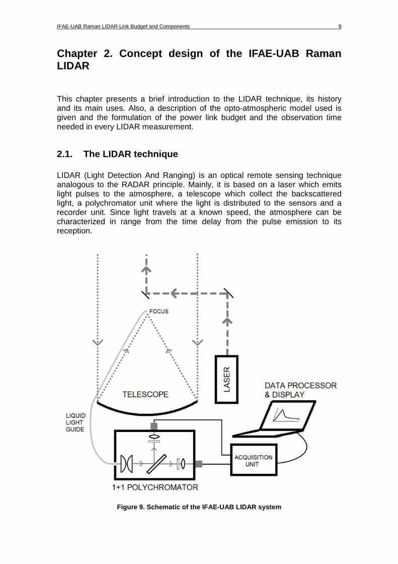
2.1. The LIDAR technique LIDAR (Light Detection And Ranging) is an optical remote sensing technique analogous to the RADAR principle. Mainly, it is based on a laser which emits light pulses to the atmosphere, a telescope which collect the backscattered light, a polychromator unit where the light is distributed to the sensors and a recorder unit. Since light travels at a known speed, the atmosphere can be characterized in range from the time delay from the pulse emission to its reception.
Figure 9. Schematic of the IFAE-UAB LIDAR system

10 Chapter 2. Concept design of the IFAE-UAB Raman LIDAR
LIDAR belongs to the remote sensing family techniques. Bats make use of a perceptual echolocation system by the emission of ultrasonic sounds. They compare returning echoes with the outgoing pulses and they are able to reproduce images of surroundings from them. During the 1930s the first invention based on this principle appeared, the SONAR, and it was used for underwater detection. A few years later, during World War II, the RADAR system was developed by the British to protect their borders, by means of microwaves capable to detect targets at large distances. The use of light for detection dates back to the 1930s, where searchlights were used to measure air density profiles. Also, in 1938, cloud base heights were measured by means of pulses generated by flashlamps. The first LIDAR system appeared in the 1960s [7] and was used to measure of Lunar to Earth distance. It was one of the first times the revolutionary invention of the LASER was used. In the 1970s, NASA started doing research about airborne LIDAR prototypes for eventual space borne sensor deployment. But, it was only with the deployment of Global Positioning Systems (GPS), ten years later, that an accurate positioning of the aircraft made the airborne surveying possible. From this time, numerous airborne and space borne missions incorporate LIDAR systems. Also ground based observations made use of this technique like in the EARLINET project [8], a network of LIDAR ground bases for aerosol observation at continental scale. Usage of a LIDAR When the laser beam interacts with the atmospheric components (aerosols and molecules), the light is scattered in all directions. A small part of this light is scattered back to the telescope and collected. Nowadays, the analysis of these data is useful in many fields as for instance in cartography, topography, agriculture, forestry, archeology and pollution modeling, as well as in navigation systems or police laser speed detectors [9]. In the last years several technologies have raised besides the pure use of elastic LIDARs. By the time of this paper, the main techniques are following: Elastic LIDAR is the simplest technique and provides information about the atmosphere constituents, aerosols, clouds, etc. The word ‘elastic’ stands for the interaction with particles and molecules where the incident and backscattered light have the same wavelength. Inelastic Raman LIDAR is usually employed parallel to elastic LIDAR measurements. When the light interacts with molecules, part of this light is backscattered with a wavelength shift characteristic of every type of molecule. By analyzing this returned power it is possible to determine the gas concentration in range. It is also possible describe the temperature of the atmosphere in range measuring the inelastic returned power. Differential Absorption LIDAR (DIAL) is used for measurement of gas concentration such as ozone, carbon dioxide or water vapor. DIAL

IFAE-UAB Raman LIDAR Link Budget and Components 11
measurements rely on the unique “fingerprint” absorption spectrum of each molecule. Two measurements are made, one at wavelength where the gas under study presents a peak of absorption, and a second at wavelength in the region of low absorption. The differential absorption between two wavelengths gives the concentration of the gas as a function of range. Doppler LIDARs are used for wind speed and direction measurements. The idea is the same as in the Doppler RADAR, that makes use of frequency shifts of the backscattered signal to determine the speed of the target. LIDARs do not operate with radio wavelength but with shorter wavelengths. In that way, RADARs are sensitive for larger targets such as rain drops or birds, while LIDARs are sensitive to aerosol particles. Inelastic interaction. The Raman LIDAR technique The fraction of light scattered by an element towards the light source will be called from now on backscattered light. As the light goes on through the atmosphere, it scatters continuously and the transmitted light becomes weaker and weaker. This last fact will be referred along this document as the extinction of the light. LIDARs can provide range-resolved profiles of the backscatter and extinction coefficients needed to characterize the atmosphere. These coefficients depend on the significant spatial variation in the particle composition and size distribution, especially in the Planetary Boundary Layer (PBL). The problem of extracting the backscatter and extinction coefficients from one measurement can be overcome taking independent measurements with a Raman LIDAR along the line of sight of the elastic LIDAR.
Figure 10. Overview of lidar backscatter signals fo r a laser wavelength of 532 nm. Adapted from [10].

12 Chapter 2. Concept design of the IFAE-UAB Raman LIDAR
The Raman LIDAR technique has turned out to be a very stable and reliable tool thanks to the improvements achieved in the interference filters and high power lasers over the last years [11]. It makes use of the weak inelastic scattering of light by atmospheric molecules. When molecules are exposed to a light source, different rotational and vibrational molecular energy levels are excited. This excitation changes the quantum state of a molecule and shifts the frequency of the scattered photon. The spectrum plotted by Raman lines for an excitation wavelength of 532 nm can be seen in Figure 10. If a high energy level is excited, the molecule absorbs energy and the frequency of the scattered photon is decreased. Inversely, the wavelength is increased. The former inelastic process is called Stokes Raman scattering. In contrast, if the energy level is lower the molecule transfers this energy to the scattered photon decreasing its wavelength. These processes are called the anti-Stokes lines. The unshifted return from the laser is the Cabannes line, which concentrates the highest power. Every Raman band or signal is characteristic of every type of scattering molecule. Their central line is called Q branch and the power concentrated at this spectral line is several orders of magnitude higher than their side bands. There has been much research on this field, and many applications that filter and use different parts of the cited spectrum have been developed. For example, measurements of atmospheric temperature are possible by analyzing the pure rotational Raman spectrum, which are the side bands around the Cabannes line. Raman process results in a frequency shift of the laser wavelength depending on the aerosol under study. Nitrogen has been used in all the Raman application because it is the major atmospheric component. The returned power after the nitrogen Raman scattering when it is exited by a wavelength light source is given at the wavelength
λ = λ1 − λ · κ, (1)
where κ is the wavenumber (2331 cm-1 for N2) [12]. The IFAE-UAB Raman lidar will take measurements from the elastic and Nitrogen Raman scattering return. From here on we will assume that the Raman channel is centered at the wavelength equal to 387 nm and and stands for the source wavelength 355 nm.
2.2. Power link budget In a lidar, a train of light pulses is emitted into the atmosphere, the telescope collects the scattered light in the same direction and the data are processed after the detector. In between, different subsystems such as the light guide, lenses, detectors or the even transient recorders take an important role in determining the figure of merit of the whole system. The estimation of the

IFAE-UAB Raman LIDAR Link Budget and Components 13
received power and signal-to-noise ratio can be useful in the appropriate selection of the different devices and provides information about the maximum range, spatial resolution and the observation time needed for the measurements.
2.2.1. Opto-atmospheric parameter modeling Elastic received power is produced by both molecular and aerosol scattering while the Raman received power is produced only by molecular interaction with the molecule of interest and therefore molecular scattering. Nevertheless, light propagation is always affected by extinction processes due to the interaction with molecules and particles. In order to estimate backscattering and extinction coefficients we have assumed a standard atmospheric model for the aerosol and molecular components hereafter described: Aerosol component (Mie scattering) A very simple wavelength dependent model has been taken for Mie backscattering processes in which aerosols are homogeneously distributed up to the Planetary Boundary Layer (PBL, considered here at 3km). Beyond the PBL, a purely molecular atmosphere is considered. Extinction component is computed from Koshmieder’s relationship [13]
532 = . !", (2)
being VM the Visibility Margin and for clear sky, that for the reference wavelength of 532 nm is approximately 39.12 Km [14]. From here on, indexes ‘aer’ and ‘mol’ stand for aerosol scattering and molecular scattering respectively. The extinction coefficient is scaled to the wavelength of interest#, whether 355 nm or 387 nm, using the equation (3). $ is the Angström coefficient which has been considered unitary [15].
%& = ' ()*+ %,-. (3)
The aerosol elastic backscattering coefficient is related to the aerosol extinction coefficient by
/%0 = 12034567 !89!" ,
(4)
where SM is the lidar ratio. Extracted from the look-up table of [14], SM is around 25.

14 Chapter 2. Concept design of the IFAE-UAB Raman LIDAR
Molecular component (Rayleigh scattering) The molecular height-dependent extinction coefficients have been simulated by using an atmospheric model provided by the RSlab department of UPC, based on the U.S. standard atmospheric model [16] which is defined for a ‘standard air’ [17]. This model accounts for the height dependent refractive index and the dry-air molecular number density. The molecular elastic backscattering coefficient is given by the Rayleigh ratio
/%0:;<= = >?α%0:;<R , (5) On the other hand, the inelastic Raman scattering is only produced by the species under study so that the inelastic backscattering coefficient depends on the nitrogen molecular number density, which is about 78% of the dry-air molecular number density. The inelastic backscattering coefficient can be written as
/%B:;<= = CD.= EF2BGEH ,
(6)
where CD. is the N2-molecule number density depending on height, IJ%BK IL⁄ is the N2-Raman backscattering differential cross-section (23.15·10-35 [m2sr-1] at 387 nm). The molecular scattering cross section is proportional to λ-4 [11] and this is the mean reason why usually small emission wavelengths are preferred. Finally, Mie and Rayleigh extinction coefficients for elastic and inelastic processes are plotted in Figure 11.
Figure 11. Simulated range dependent aerosol (Mie) and molecular (Rayleigh) extinction coefficients.
0 5 10 15 0
0.02
0.04
0.06
0.08
0.1
0.12
0.14
0.16
Ext
inct
ion
[km
]
Altitude [km]
α
Mi e 387 nm α
Mi e 355 nm α
Ray 355 nm α
Ray 387 nm
Elastic/Raman Mie and Rayleigh extinction
IFAE-UAB Raman LIDAR Link Budget and Components 15
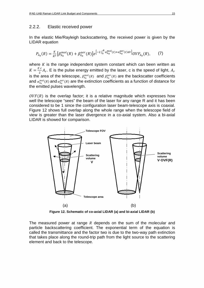
2.2.2. Elastic received power In the elastic Mie/Rayleigh backscattering, the received power is given by the LIDAR equation
N%0= = O. P/%0:;<= + /%0=RST!U VW0XYZ[\VW0]^_[EB0 `abc%0=, (7)
where is the range independent system constant which can been written as = de
f. E is the pulse energy emitted by the laser, c is the speed of light, f is the area of the telescope, /%0:;<= and /%0= are the backscatter coefficients and %0:;<=and %0= are the extinction coefficients as a function of distance for the emitted pulses wavelength. abc= is the overlap factor; it is a relative magnitude which expresses how well the telescope “sees” the beam of the laser for any range R and it has been considered to be 1 since the configuration laser beam-telescope axis is coaxial. Figure 12 shows full overlap along the whole range when the telescope field of view is greater than the laser divergence in a co-axial system. Also a bi-axial LIDAR is showed for comparison.
(a) (b)
Figure 12. Schematic of co-axial LIDAR (a) and bi-a xial LIDAR (b)
The measured power at range = depends on the sum of the molecular and particle backscattering coefficient. The exponential term of the equation is called the transmittance and the factor two is due to the two-way path extinction that takes place along the round-trip path from the light source to the scattering element and back to the telescope.
Telescope area
Telescope FOV
Scattering volume V
Scattering volume V·OVF(R)
Laser beam

16 Chapter 2. Concept design of the IFAE-UAB Raman LIDAR
2.2.3. Raman received power Analogously, the received power in the Raman channel can be written as
N%B= =O. /%B:;<=S!U T120ghi\120345\12Bghi\12B345E`B0 abc%B=, (8)
where K is the system constant. abc= is the overlap factor and it is unitary along the whole range R since the co-axial configuration of the LIDAR. The backscattering and extinction coefficients are computed in the previous section. In contrast with the elastic received power, Raman process is produced only by molecules and it just depends on the inelastic backscattering coefficient (equation (6)). Furthermore, the light extinction takes place in different wavelengths in the round trip. LASER light (at 355 nm) is extinguished by molecules and aerosols ( %0j9 and 0#S9) along its way. After being backscattered by the nitrogen at the distance R and at 387 nm, it returns to the telescope being again extinguished by both molecules and aerosols ( %lj9 and =#S9).
2.2.4. Background received power The function of the telescope is to collect the laser light backscattered in the atmosphere. But even when the laser is off, the telescope collects light from the sky. The power received in such condition is called background power and it should be lower than the signal light. It has been a challenge for daytime Raman LIDARS but high power lasers and very narrow filters developed in the last years have overcome this problem. The background power is given by
Nme+ = nmfILI, (9) where Lb is the irradiance from the sky, f is the telescope area, IL is the solid angle computed from the telescope field of view and dλ is the interference filter bandwidth in every channel. For the case of the IFAE-UAB lidar, the elastic and Raman channel have the same filters and thus they receive the same background power. The Raman LIDAR that is under development will work in La Palma solely at night. For that reason, the irradiance of the night sky was measured in [18] and is 2.72·10-13 [W·cm-2·nm-1·sr-1]. The LIDAR will be always pointing at different directions in the night sky but under no circumstances towards the moon. That will decrease significantly the power received from the background simplifying the design of the system.
IFAE-UAB Raman LIDAR Link Budget and Components 17
2.2.5. Channel transmissivity The channel transmissivity ( 10 ≤≤ ξ ) is defined as the product of the individual subsystem transmission factors (i.e., the inverse of the optical losses) along the optical receiving chain. Formally,
( ) ( ) ( ) ( ) ( )λξλξλξλξλξ polygPSFT= , (10) where Rλλλ ,0= is the elastic/Raman reception wavelength, ( )λξT is the
telescope transmission, ( )λξg is the liquid-guide transmission, ( )λξPSF is the
guide-to-telescope coupling efficiency due to the PSF of the telescope (Sect. 3.2), and ( )λξ poly is the total polychromator transmission defined as
( ) ( ) ( ) ( )λξλξλξλξ IFn
lensdichrpoly = , (11)
where ( )λξdichr , ( )λξlens , and ( )λξIF are the dichroic mirror (D1), lenses (L1-L4), and interference-filter transmission factors, respectively, described later in Table 4 Section 4.1 . In Equation (11), 3=n for all the lenses (L1-L4) in each channel of the polychromator are assumed identical transmissivities. The elastic/Raman channel transmissivities, according to Equation (10), are listed in Table 1 along with the channel voltage responsivity (or net voltage responsivity),
( ) ( ) ( )λξλλ Tiv GRR =′ , (12)
defined as the product of the current responsivity of the detector, iR [A/W], times
the transimpedance gain TG ( Ω== 50inT RG , i.e., the input impedance of the
transient recorder), times the channel transmissivity, ( )λξ from (10) above.
2.2.6. Signal-to-noise ratio Every element in the system can act as a noise source, resulting in a bad detection of the light received. But some of these are more relevant than others, thus limiting the LIDAR performances. In these systems the predominant noise comes usually from the photomultiplier tube (PMT). When light enters the photocathode (the sensitive part of the PMT), electrons are emitted and multiplied by a secondary electron emission through the dynodes, and these are collected by the anode as an output pulse. If incident light is strong, these pulses are so close in time that the processing circuit is not fast enough and they overlap creating an analog current with shot noise fluctuations [19]. In this situation, the only way to analyze this continuous current is by using what is known as Analog Mode. In contrast, when the light intensity is weak, pulses are detected individually. Since detected pulses

18 Chapter 2. Concept design of the IFAE-UAB Raman LIDAR
undergo binary processing for digital counting, this method is known as digital mode or photon-counting mode. Inelastic received power is around 3 orders of magnitude lower than the elastic one, due to the low cross sections of Raman scattering. That is the reason why Raman LIDARs need high power lasers, large telescopes, long integration times and they are mostly used for gases with high molecular concentrations. The results given in this paper assume analog detection for the elastic channel and photon counting mode for the Raman channel whilst the acquisition module records both at the same time. Depending on the energy level of the signal it is used digital or analog data, and in the region in between the system uses a “gluing” algorithm that can increase the final SNR. Signal-to-noise ratio for the elastic channel As stated before, the Analog Mode is used when the photons flow reaching the photocathode is so intense that the output pluses at the anode overlap and produce a continuous current with noise fluctuations. Shot noise is basically caused by 3 sources:
• Shot Noise Resulting from Signal Light: Since the secondary electron emission in a photomultiplier tube occurs with statistical probability, the resulting output also has statistical fluctuation.
• Shot Noise Resulting from Background Light: It is generated in the same
way as the shot noise resulting from the signal light.
• Shot Noise Resulting from Dark Current: Even when there is no light entering the photocathode an output current is observed. This dark current is mainly caused by thermionic emission from the photocathode and dynodes.
These three noise components and the thermal noise added by the acquisition unit have associated noise spectral densities that can be computed as
Jpq,p = = 2rstcu=(;N=v wb
xyz, (13)
Jpq,m = 2rstcu=(;Nme+v wb
xyz, (14)
Jpq,E = 2rstcuEm wb
xyz, (15)
J|q = 4$~=( wb
xyz, (16)

IFAE-UAB Raman LIDAR Link Budget and Components 19
where st is the transimpedance channel gain [V/A] (i.e., the acquisition unit input impedance, st = =( = 50Ω), c is the photomultiplier excess noise factor [dimensionless units], u is the PMT multiplication factor or gain, =(; is the cathode radiant sensitivity [A/W], N= is the return power [W], Nme+ is the background-radiation power [W], v is the net optical transmissivity [dimensionless units], Em is the bulk-dark current [A], r is the electron charge [C], k the Boltzmann’s constant [J/K] and ~ = 300K is the noise equivalent temperature. These variances are expressed as noise spectral density and they have to be multiplied by the noise equivalent bandwidth D= 10 [MHz] to compute the SNR. Then the signal to noise ratio takes the form
C=== =(;ustvN=2rstcu=(;vN= + Nme+" + 2rstcuEm + 4$~=("D
bb (17)
Then, if the thermal noise is much lower than the other noise sources it is safe to conclude that the SNR does not depend either on the multiplication factor of the PMT or on the transimpedance channel gain since they cancel out in the equation (17) . Signal to noise ratio for the Raman channel Photon counting mode is used when the number photons entering into the photocathode is so low that output pulses can be detected as separate pulses. In this mode we find the same three noise sources as the ones in the analog mode, but variances are computed in counts per second. They can be computed as N = P[L[R q⁄ counts/sec", (18)
N = PL[R q⁄ counts/sec", (19)
N = I q⁄ counts/sec", (20)
where N is the number of photo-induced counts from signal light per second, Nis the number of photo-induced counts from the background light per second and N is the number of photo-induced counts from the dark-current per second. Then the SNR in photon counting mode is
where τ the fraction of time is where the photo-counter is adding counts (considered 100 ns to achieve the same spatial resolution than in Analog Mode)
SNRR = NR√τ¡NR + 2N + N
, (21)
20 Chapter 2. Concept design of the IFAE-UAB Raman LIDAR
2.2.7. Integration time As it has been discussed in Chapter 1, the goal of building this LIDAR is to improve the quality of data taken with ground-based Cherenkov telescopes. They work independently and the Raman LIDAR should not interfere with astronomical data acquisition, that can be achieved by using the dead time between two subsequent measurement campaign when the telescopes is repointing. The integration time is the time needed for the LIDAR in one observation to get the necessary SNR. Thus, this time turns into a key parameter in trade-off with the maximum range. Pulse integration is commonly used in many detection systems to improve the signal received, by degrading the range resolution. When N pluses are integrated, the signal to noise ratio is improved by square root of N. Thus, the number of pulses to integrate is
N = ¢SNR£¤SNR≏ ¦ (22)
where SNR≏ is the signal to noise ratio of a single pulse, SNR§ is the minimum needed signal to noise ratio and N must be a rounded up integer. Then, the observation time needed to integrate enough pulses to fulfill the detection condition is
t¨ = N
PRF (23)
And equivalently using equations (22) and (23)
t¨ = 'SNR£¤SNR≏
*
· 1PRF (24)
where SNRgoal is the minimum Signal-to-Noise Ratio required by the inversion algorithm used, which will be defined at a later time of the project. In our case a ratio of 10 has been used. To stand out the importance of the inversion algorithm, Figure 13 shows the observation time needed versus range. For the same LIDAR system, two different inversion algorithms are considered in this plot, being the related SNRgoal equal to 1 (blue line) and equal to 10 (red line). The SNR needed is increased a factor of 10, resulting in an increase of the observation time by a factor of 100 for the same range. With this implication, a system that normally needs a few seconds to take measurements would need a few minutes if a different algorithm is used.

IFAE-UAB Raman LIDAR Link Budget and Components 21
Figure 13. Lidar altitude versus observation time f or SNR goal equal to 1 and equal to 10
In a similar way, any improvement in the SNR by a factor of ζ reduces the observation time a factor of ζ as this
t¨′ = NPRF = 'SNR£¤ζ · SNR≏*
· 1PRF (25)
or in short
t¨′ = t¨ζ (26)
From here on, all the simulations are made with a SNRgoal equal to 10. If it is improved in the inversion stage, the observation times given in this document can be recomputed easily with the equation (21). 2.3. Performance assessment of the IFAE-UAB LIDAR The power link budget of our LIDAR consists on the range-resolved computation of the received power. This is useful to evaluate the optical losses of the system, the SNR at the receiver, the observation time needed to take atmospheric measurements up to a desired range and how the different components of the LIDAR affect the performance.
10
-2
10
-1
10
010
110
210
-1
10
0
101
102
Observation time [sec]
Alti
tude
[km
]
Maximum system altitude Vs Observation time
SNRgoal = 1
SNR = 10 goal

22 Chapter 2. Concept design of the IFAE-UAB Raman LIDAR
EMITTER
LASER
Type Model Emitted wavelength, λ Energy per pulse, E Pulse Repetition Frequency, PRF Beam waist (diameter) Beam Divergence, θ Pulse duration, τp
Nd:YAG Quantel Brilliant 355 nm 60 mJ 20 Hz 6 mm 0.5 mrad 5 ns
RECEIVER
Telescope
Geometry Diameter, d Shadow diameter, dsh Focal length, f Transmissivity, ξT
Parabolic mirror 1.8 m 0.08 m 1.8 m 0.55
Liquid-guide-to-telescope coupling efficiency, ξPSF 0.9
Liquid Guide
Manufacturer & Model Active area diameter, db Numerical Aperture, NA Transmissivity, ξg
Lumatec Series 300 8 mm 0.59 (34º half-angle) >0.7 (in the UV)
Photodetectors Type Active area diameter, db PMT model
PMT 22 mm Hamamatsu R1924A
Acquisition unit (transient recorder)
Type Model
Mixed analog-to-digital converter (ADC) / Photon counter (PC) ADC 20 Msps 12bit / 250-MHz PC LICEL TR20-160
CHANNEL SPECIFICATIONS Wavelength [nm] 355 387 (N2) Type Elastic Raman Resolution [m] Up to 15 m in analog mode (10-MHz bandwidth), up to 7.5 m in
photon-counting mode (50-ns bin)
Polychromator TX, ξpoly (Eq.(11))
0.90×0.903×0.60 = 0.39 0.90×0.903×0.65 = 0.43
Channel transmissivity, ξpoly (Eq.(11))
0.15 0.16
Channel responsivity, vR′ [V/W] 8.0×10⁵ 8.7×10⁵
Spectral Bandwidth, ∆λ [nm] 10 10 Type of Detector PMT PMT Model R1924A (Hamamatsu) R1924A (Hamamatsu) Transimpedance gain (input impedance of the transient recorder) [Ω]
50 50
Internal Gain, M 2x10⁶ 2x10⁶ Noise Factor, F 1.8 1.8 Current responsivity, Ri [A/W] 1.1x10⁵ 1.1x10⁵
Dark current, Id [nA] 3 3
Table 1. Specifications of the lidar system
To evaluate the equations exposed in Chapter 2 we have programmed a MATLAB script. The plots simulated in this chapter illustrate the importance of the subsystem parameter choice in the link budget. Table 1 shows the parameters of the IFAE-UAB LIDAR.

IFAE-UAB Raman LIDAR Link Budget and Components 23
The received power in the elastic and Raman channel is showed in Figure 14, as well as the power received from the background; computed with equations (7), (8) and (9). Thus proving, that background power is about two orders of magnitude lower than the Raman received power at 15km.
Figure 14. Received Power versus altitude
Figure 15(b) shows that signal shot noise variances in the elastic and Raman channel are above other noise variances. This is due to the large size of the telescope and the low irradiance of the night sky, and therefore the system will be dominated by signal shot noise minimizing the role of other noise sources.
Figure 15. (a) Variances of signal shot noise, dark current shot noise and background noise versus range for the elastic channel. (b) Var iances of signal shot noise, dark current shot noise and background shot noise versus altitude for the Raman channel.
0 5 10 15 10
-12
10-10
10-8
10-6
10-4
10-2
Altitude [km]
Pow
er[W
] Power received by the telescope
355 nm
387 nm
P b a c kgro und
0 5 10 15
104
106
108
1010
1012
Noi
se v
aria
nce
[cou
nts/
sec]
Signal shot noise
Dark shot noise
Background shot noise
Noise variances Raman ch. (387 nm), PC detection
Altitude [km] (b)
0 5 10 15
10-10
10-5
100
Altitude [km](a)
Noi
se v
aria
nce
[V2 ]
2
Noise variances elastic ch. (355 nm), analog detection
Signal shot noise
Dark shot noiseBackground shot noise
Thermal noise

24 Chapter 2. Concept design of the IFAE-UAB Raman LIDAR
Figure 16. SNR for elastic (355nm) and Raman (387nm ) Channel
SNR for a single pulse is plotted in Figure 16. Several pulses can be integrated to achieve a required SNR. In that case, the observation time has been calculated from (25) and is plotted in Figure 17 for the most restrictive case (SNRgoal = 10). Since the received power in the elastic channel is around 3 orders of magnitude higher than in the Raman channel, it is safe to say that the observation time for the whole system will be determined by the Raman channel restrictions, as it is showed in Figure 17.
(a) (b)
Figure 17. Observation time versus Range for a mini mum required SNR of 10. (a) Plotted in logarithmic scale (b) Plotted in linear scale
About 77 seconds are needed to get data from up to a 15km high and 27.5 seconds to reach the typical altitude (12km) where the EAS take place. However, the time to take measurements up to a certain altitude increases when the lidar is not pointing vertically but with some angle θ respect to the zenith direction. The range increases with θ and also the number of aerosols and molecules that interact with the LASER beam (Figure 18a). That effect can be seen in Figure 18b for a constant height of 12km.
0 5 10 15
100
102
104
Altitude[km]
SN
R [
]
Signal to noise ratio
355 nm
387 nm
0 5 10 150
20
40
60
80
Altitude [km]
Obs
erva
tion
time
[s]
Max. system range Vs Obs. time
387 nm
355 nm
10-2
10-1
10 0 101
102
100
101
Alti
tude
[km
]
Observation time [s]
Max. system Range vs. Obs. time
355 nm 387 nm

IFAE-UAB Raman LIDAR Link Budget and Components 25
(a) (b)
Figure 18. Sketch of the laser beam pointing to a d irection different form Zenith (a) and plot of the observation time versus the angle of ob servation respect to Zenith to reach a height of 12km (b)
By limiting the observation we can compute the maximum angle of observation. For instance, if our system averages pulses for 100 seconds, which is a typical time [11], atmosphere characterization will be possible within a radius of 16km.
0 10 20 30 40 500
100
200
300
400
500
θ [Degrees]
Obs
erva
tion
time
[sec
]
Observation time VS Angle of observation

26 Chapter 3. System details and parameterization of the obs. time for different subsystem configurations
Chapter 3. System details and parameterization of t he observation time for different subsystem configurations The LIDAR system must be optimized for the project needs by choosing the correct components. A brief description about the devices that compose IFAE-UAB LIDAR is detailed next, as well as the parameters that take an important role in the power link budget.
3.1. LASER The LIDAR we will be using is equipped with a Nd:YAG laser from Brilliant. The fundamental wavelength of the laser is 1064 nm and third harmonic generation (THG) is used to produce light at a 355nm wavelength. Main parameters can be found in Table 1. It is the cheapest commercial solution for atmosphere characterization at the wavelength where EAS take place (peak energy at 330 nm). The laser also emit at 532 nm by second harmonic generation. This option could eventually be used to characterize the atmospheric transmission at both ends of EAS spectrum by adding two more channels to the LIDAR.
PRF (Hz) 10 20 50
Energy per pulse (mJ) 65/100 60/70 20
Table 2. Energy per pulse for different pulse repet ition frequencies
For the same average power, higher pulse energy at a lower pulse repetition rate is preferred because SNR is improved in this way [11]. This laser can work with 3 Pulse Repetition Frequencies; 10Hz, 20Hz and 50Hz. The energy per pulse is different in all of them and for 10Hz and 20Hz an extra option to increase the energy is available (see Table 2). The lowest observation time (see Figure 19) is achieved by using a PRF equal to 20Hz. As the observation time in the standard mode (with 60mJ per pulse) and in the special mode (with 65mJ per pulse) are very similar, a low energy per pulse is preferred to extend the laser’s life.
Figure 19. Observation time versus range for differ ent laser settings (min. SNR of 10)
0 5 10 150
20
40
60
80
100
Range[km]
Obs
erva
tion
time
[s]
Different settings of the laser
10Hz - 65mJ
10Hz - 100mJ
20Hz - 60mJ20Hz - 65mJ
50Hz - 20mJ

IFAE-UAB Raman LIDAR Link Budget and Components
The laser beam is guided beam coaxially to the telescope into the atmosphere. Its divergence is lower than the telescope field of view, expanders [11].
3.2. Telescope The telescope is one of the Cherenkov light in La Palma and it will be reused for the some modification in the mechanics. meters as well as its focal length. ItLIDAR system but, since the irradiance of the night sky in La Palma is very lowcompared to night sky in urban areasthe link budget simulations that collected from the background
The mirror transmissivity was meaPoint Spread Function was telescope with a Gaussian distribution4mm radio circle [21]. This telescope because they condition On a first approach, Background and dark current noise can be neglectedSNR in photon counting mode if the system ias it is the case (see Figure
SNR « ¡P[ξ®R SNR increases by the square root of the telescopewith its diameter. Therefore
UAB Raman LIDAR Link Budget and Components
m is guided with two flat mirrors, as shown in Figure beam coaxially to the telescope into the atmosphere. Its divergence is lower than the telescope field of view, thus there is no need for using beam
is one of the set that CLUE project (1987-2002) had to measure Cherenkov light in La Palma and it will be reused for the IFAE-UABsome modification in the mechanics. The diameter of the parabolic mirror is 1.8 meters as well as its focal length. Its dimensions are quite large for
since the irradiance of the night sky in La Palma is very lowcompared to night sky in urban areas, it has been shown (see Figure the link budget simulations that the system is not dominated by the power collected from the background.
Figure 20. View of the telescope
sivity was measured in [20] and it is about 50was measured. Light arrive to the focal plane of the
Gaussian distribution in which the 90% of the light falls in a . This high PSF is the main drawback of
because they condition the polychromator unit’s optic design.
Background and dark current noise can be neglectedSNR in photon counting mode if the system is dominated by signal
Figure 15). With this approximation
R q⁄ √τ
by the square root of the telescope’s area, or in other wordsits diameter. Therefore, every time that the telescope diameter is doubled
27
Figure 9, to emit the beam coaxially to the telescope into the atmosphere. Its divergence is 4 times
thus there is no need for using beam
had to measure UAB LIDAR after
of the parabolic mirror is 1.8 large for a typical
since the irradiance of the night sky in La Palma is very low Figure 15) with
system is not dominated by the power
and it is about 50-60%. Also the . Light arrive to the focal plane of the
ich the 90% of the light falls in a is the main drawback of reusing this
optic design.
Background and dark current noise can be neglected from s dominated by signal shot noise,
(27)
in other words, , every time that the telescope diameter is doubled,
28 Chapter 3. System details and parameterization of the obs. time for different subsystem configurations
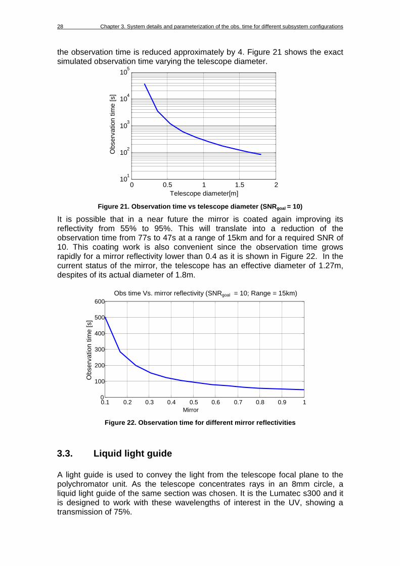
the observation time is reduced approximately by 4. Figure 21 shows the exact simulated observation time varying the telescope diameter.
Figure 21. Observation time vs telescope diameter ( SNRgoal = 10)
It is possible that in a near future the mirror is coated again improving its reflectivity from 55% to 95%. This will translate into a reduction of the observation time from 77s to 47s at a range of 15km and for a required SNR of 10. This coating work is also convenient since the observation time grows rapidly for a mirror reflectivity lower than 0.4 as it is shown in Figure 22. In the current status of the mirror, the telescope has an effective diameter of 1.27m, despites of its actual diameter of 1.8m.
Figure 22. Observation time for different mirror re flectivities
3.3. Liquid light guide A light guide is used to convey the light from the telescope focal plane to the polychromator unit. As the telescope concentrates rays in an 8mm circle, a liquid light guide of the same section was chosen. It is the Lumatec s300 and it is designed to work with these wavelengths of interest in the UV, showing a transmission of 75%.
0.1 0.2 0.3 0.4 0.5 0.6 0.7 0.8 0.9 10
100
200
300
400
500
600
Mirror
Obs
erva
tion
time
[s]
Obs time Vs. mirror reflectivity (SNRgoal = 10; Range = 15km)
0 0.5 1 1.5 2 10 1
10 2
10 3
10 4
10 5
Telescope diameter[m]
Obs
erva
tion
time
[s]

IFAE-UAB Raman LIDAR Link Budget and Components 29
The numerical aperture was measured in the IFAE laboratory. This measurement shows the dependency between the angle of incident light and the outgoing light angle. The light condensed by the telescope enters into the fiber with a maximum angle of arctang (1.8/0.9) = 26.57º deg. For this angle of aperture of the liquid guide results to be 34º (half angle).
3.4. Polychromator unit In the polychromator unit, the light is distributed from the light guide to the different sensors. For such purpose, a set of lenses, a dichroic mirror, and interference filters are used. Initially, the box is composed by two sensors but it has been designed to eventually accept more channels with the minimum changes possible. A description of the proposal design for the polychromator unit can be found in Chapter 4.
3.5. Photomultiplier tubes The most commonly used sensors for the UV frequencies are Photomultiplier Tubes (PMT’s). As explained in section 2.2.4, they are composed by a photocathode, a set of dynodes and an anode. For every photon that reaches the photocathode ƞ electrons are emitted and multiplied by secondary electron emissions through the dynodes, being ƞ the PMT quantum efficiency. Between all the possible PMT in the market a Bialkali PMT of Hamamatsu has been chosen because they have higher quantum efficiency at the UV wavelengths than other sensors. The R1924A PMT shows its quantum efficiency peak (25%) at wavelengths of 350-400nm.
Figure 23. Section sketch of a PMT [22]
There exist a range of PMTs of different diameters for UV wavelengths. It is advisable to choose the smallest one possible to reduce the anode dark current. Nevertheless, the design of the polychromator unit is not straightforward since the aperture and section of our light guide are quite larger than desirable. Even if it is possible to use PMTs of 8mm for the two first channels, the following PMTs must be larger (See chapter 4).Therefore, we could then say that it is
30 Chapter 3. System details and parameterization of the obs. time for different subsystem configurations
preferable that all of them PMTs are from the same kind to make a hypothetical future replacement faster, easier and more efficient. Additionally, simulations with a larger one have been made. Their parameters are summarized in Table 3.
PMT model R7400U R1924A
Equivalent active area diameter [mm] 8 22
Multiplication factor [ ] 7e5 2e6
Anode dark current [nA] 0.2 3
Anode radiant sensitivity [mA/W] 60 55
Table 3. R7400U and R1924A parameters
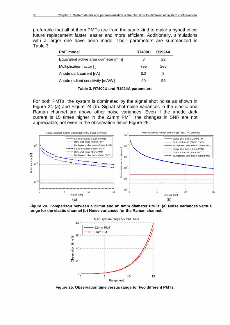
For both PMTs, the system is dominated by the signal shot noise as shown in Figure 24 (a) and Figure 24 (b). Signal shot noise variances in the elastic and Raman channel are above other noise variances. Even if the anode dark current is 15 times higher in the 22mm PMT, the changes in SNR are not appreciable; not even in the observation times Figure 25.
(a) (b)
Figure 24. Comparison between a 22mm and an 8mm dia meter PMTs. (a) Noise variances versus range for the elastic channel (b) Noise variances f or the Raman channel.
Figure 25. Observation time versus range for two di fferent PMTs.
0 5 10 15
10-10
10-5
100
Altitude [km]
Noi
se v
aria
nce
[V2 ]
Noise variances elastic channel (355 nm), analog detection
Signal shot noise (22mm PMT)Dark shot noise (22mm PMT)
Background shot noise (22mm PMT)
Signal shot noise (8mm PMT)
Dark shot noise (8mm PMT)Background shot noise (8mm PMT)
0 5 10 1510
2
104
106
108
1010
1012
Altitude [km]
Noi
se v
aria
nces
[co
unts
/sec
]
Noise variances Raman channel (387 nm), PC detection
Signal shot noise (22mm PMT)Dark shot noise (22mm PMT)
Background shot noise (22mm PMT)
Signal shot noise (8mm PMT)
Dark shot noise (8mm PMT)Background shot noise (8mm PMT)
0 5 10 150
20
40
60
80
Range[km]
Obs
erva
tion
time
[s]
Max. system range Vs Obs. time
22mm PMT
8mm PMT

IFAE-UAB Raman LIDAR Link Budget and Components 31
To avoid over passing the maximum current of the photocathode a gated PMT solution (i.e., including an electronic enable/disable feature) will be used to disable reception during the first 200 m of the LIDAR signal where, due to the laser-telescope coaxial arrangement, the detectors become blinded. For the elastic channel, it is envisaged inclusion of neutral density filters to accommodate the return power levels to levels comparable to those of the Raman channel, since with such a large-aperture telescope, the input light levels can drive the PMT detector deep into saturation.
3.6. Transient recorder The output current from the PMTs is acquired by a transient recorder LICEL TR20-160. The signal is recorded simultaneously by an Analog to Digital Converter (ADC) of 12 Bits at a sampling rate of 20 MSamples/sec and a discriminator which detects voltage pulses above a selected threshold (See Figure 26).
Figure 26. Schematic setup of the LIDAR trancient r eceiver TR20-160 [23]
For analog detection the signal is amplified, according to the input range selected, and signals below a frequency of 10MHz are passing the anti-alias filter to be digitized by a 12 bit ADC. Each signal is written to a fast memory which is readout after each shot and added to the summed signal in a RAM. Depending on the trigger input on Trigger A or trigger B the signal is added to ram A or B, which allow acquisitions of to repetitive channels if these signals can be measured sequentially. At the same time the signal part in the high frequency domain above 10MHz is amplified and a 250 MHz discriminator detects single photon events above the selected threshold voltage. Two different settings of the preamplifier can be controlled by software together with 64 different discriminator levels. Again the signal is written to a faster memory RAM after each acquisition cycle. An acquisition system using the TR20-160 can be configured for up to 16 simultaneous detection channels. Such a system is configured by using a HF cassette mounted transient recorder module for each channel, a rack comprising power supplies and an interface ports and a computer which.

32 Chapter 4. The polychromator unit
Chapter 4. The polychromator unit The beam light collected by the telescope contains the inelastic and elastic channels. It travels through the light guide to be filtered and detected afterwards. In an intermediate step, the different parts of the spectrum must be isolated and redirected to the correspondent sensor. This is made inside the polychromator unit, which is a box equipped with filters, lenses and mirrors to direct the light towards the PMTs. The design of the polychromator unit is critical in order to evaluate the net optical losses of the LIDAR. During this chapter, a first attempt for the polychromator unit is proposed, which aims not at describing the final components of the unit but to evaluate the necessary elements, their size and the losses of the optical paths. A first study with paraxial calculations can be formulated to determine critical parameters such as focal lengths, diameter and position of images and objects. Nowadays, any optical design cannot be conceived without the use of ray tracing simulation software. ZEMAXTM is a tool for optical engineers to design, analyze and optimize any optical system [24]. The use of this tool has helped to describe the appearance of the polychromator unit in terms of size and position of the elements used.
4.1. ZEMAXTM ray-tracing simulation Here a proposal for the polychromator unit of the IFAE-UAB Raman Lidar is presented. The proposed design for a two channel polychromator unit fits in a 26cm x15cm. Its framework has an inverted ‘T’ shape, receiving the light from the left side port and detecting elastic and inelastic channels from the top and right ports. It was designed with the intention of developing a modular unit, with the possibility of adding more channels with minimum changes. Therefore, one output port would be at the right side and the rest at the top.
Figure 27. Polychromator design layout and related ZEMAXTM ray tracing at 387 nm (elastic channel) and 387 nm (nitrogen Raman channe l). (D1) Dichroic mirror; (L1, L2, L3, L4) Lenses; (I1, I2) Interference Filters.
IFAE-UAB Raman LIDAR Link Budget and Components 33
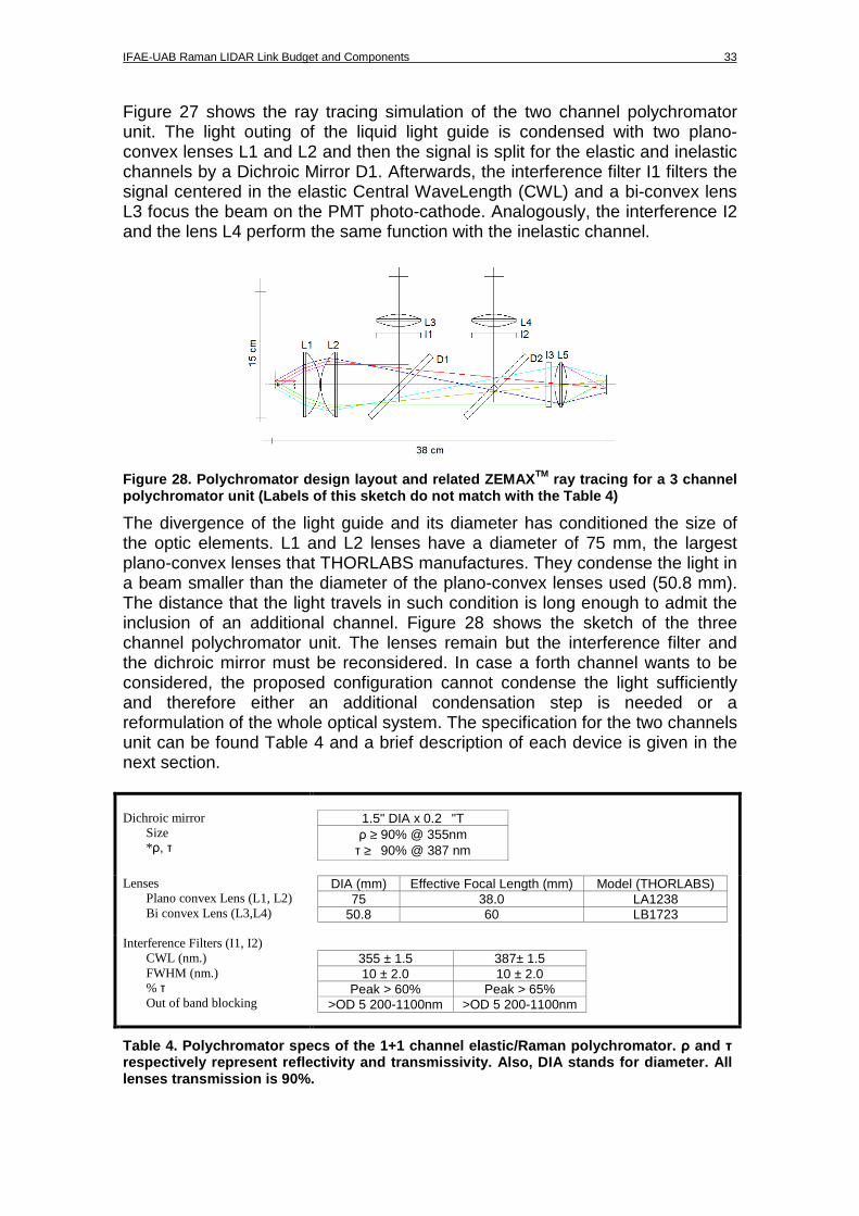
Figure 27 shows the ray tracing simulation of the two channel polychromator unit. The light outing of the liquid light guide is condensed with two plano-convex lenses L1 and L2 and then the signal is split for the elastic and inelastic channels by a Dichroic Mirror D1. Afterwards, the interference filter I1 filters the signal centered in the elastic Central WaveLength (CWL) and a bi-convex lens L3 focus the beam on the PMT photo-cathode. Analogously, the interference I2 and the lens L4 perform the same function with the inelastic channel.
Figure 28. Polychromator design layout and related ZEMAXTM ray tracing for a 3 channel polychromator unit (Labels of this sketch do not ma tch with the Table 4)
The divergence of the light guide and its diameter has conditioned the size of the optic elements. L1 and L2 lenses have a diameter of 75 mm, the largest plano-convex lenses that THORLABS manufactures. They condense the light in a beam smaller than the diameter of the plano-convex lenses used (50.8 mm). The distance that the light travels in such condition is long enough to admit the inclusion of an additional channel. Figure 28 shows the sketch of the three channel polychromator unit. The lenses remain but the interference filter and the dichroic mirror must be reconsidered. In case a forth channel wants to be considered, the proposed configuration cannot condense the light sufficiently and therefore either an additional condensation step is needed or a reformulation of the whole optical system. The specification for the two channels unit can be found Table 4 and a brief description of each device is given in the next section. Dichroic mirror
Size *ρ, τ
1.5" DIA x 0.2 "T ρ ≥ 90% @ 355nm τ ≥ 90% @ 387 nm
Lenses
Plano convex Lens (L1, L2) Bi convex Lens (L3,L4)
DIA (mm) Effective Focal Length (mm) Model (THORLABS) 75 38.0 LA1238
50.8 60 LB1723
Interference Filters (I1, I2) CWL (nm.) FWHM (nm.) % τ Out of band blocking
355 ± 1.5 387± 1.5 10 ± 2.0 10 ± 2.0
Peak > 60% Peak > 65% >OD 5 200-1100nm >OD 5 200-1100nm
Table 4. Polychromator specs of the 1+1 channel ela stic/Raman polychromator. ρ and τ respectively represent reflectivity and transmissiv ity. Also, DIA stands for diameter. All lenses transmission is 90%.

34 Chapter 4. The polychromator unit
4.2. Description of the polychromator unit componen ts Here a short description of each component in the polychromator unit is given: the light guide, the condenser lenses, the dichroic mirror, the interference filters and the eye-piece. Liquid light guide model The whole optical design is constrained by the light guide diameter and divergence (See section 3.3 for a description of the liquid light guide). As the telescope concentrates the light in an 8mm spot (with a loss of 10%) the liquid light guide used has that same size. Measurements over the light guide show that the light comes out of it with an aperture of 34º (half angle). One end receives the light from the telescope while the other one is connected to the polychromator unit, illuminating the designed paths inside it. This end can be seen as an infinite set of point sources distributed over its circular section. In order to simulate the light coming out from the light guide, we have modeled its section as 3 point sources, vertically placed and separated 4mm with the same aperture as the light guide. The main objective is to emulate the light coming out of the light beam with its 34º angle. This can be seen in the figure below:
Figure 29. Modeling of the light guide end as an in finite set of point sources (left) and simulated model with two exterior point sources whe re rotational geometry can be applied.
The Figure 29 can be inferred as the transversal section of the beam light and rotational geometry can therefore be applied. By doing so, all possible rays coming out from the light guide are covered. Condenser lens The end of the fiber cannot be considered as a point source which is an important inconvenient. A point source can be collimated with a plano-convex lens by placing it at its focal distance F (Figure 30). However, the lens is not

IFAE-UAB Raman LIDAR Link Budget and Components 35
design for collimating the light that comes from the focal plan with a certain height. As a result of the former, the rays coming out of lens are not parallel, so that they diverge. Also, the large aperture of the fiber requires large lenses placed very near to avoid the light overflow.
Figure 30. Simulation of rays coming from a point s ource at the focus of a plano-convex lens (red rays) and rays coming from the focal plan e of the lens with a certain height (blue rays).
A condenser configuration with two plano-convex lenses has been used to reduce the divergence of the beam light. It makes use of the larger lenses that Thorlabs manufactures. This configuration allows enlarging the optical paths enabling the addition of more channels (Figure 31), however by using two lenses instead of one, the transmissivity decreases from 0.9 to 0.8.
Figure 31. Ray tracing simulation for three point s ources placed at the focal plane of a plano-convex lens (above) and ray tracing simulatio n for three point sources illuminating two plano-convex lenses in a condenser configuratio n. The rays are drown up to their aperture is the same as the diameter of the eye-pie ce used.

36 Chapter 4. The polychromator unit
Dichroic mirror Elastically backscattered light in the Raman channel must be suppressed because it is around 3 orders of magnitude higher than the light in the Raman channel. In the polychromator unit, the beam light must be split in frequency and space domains in order for the beam to be detected by the PMTs: This is the task of the dichroic mirrors, tilted 45º degrees to the direction of the light propagation. These mirrors reflect the part of the spectrum below the designed wavelength upwards; and transmit forward the part of the spectrum above this wavelength (Figure 32). For instance, dichroic mirrors are used in LCD projectors to extract the red, green, and blue light from the white light and project color composed images.
Figure 32. Sketch of the ray tracing in a dichroic mirror (left) and its transmisivity depending on the wavelength (right).
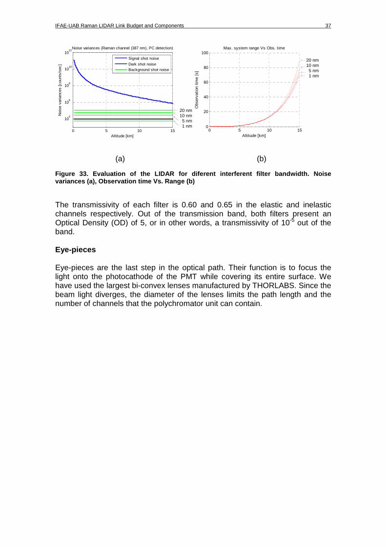
Dichroic mirrors are commonly used in visible spectrum and they are easy to find in optic manufacture’s catalogs. However, dichroic mirrors for UV wavelengths are usually manufactured by request. The manufacturer Materion is currently producing the dichroic mirror for the IFAE-UAB Raman LIDAR which transmissivity and reflectivity are larger than 90% at 387nm and 355nm respectively. This transmissivity and reflectivity have to be measured because the mirror design wavelength changes when the light incidence angle is different than 45º [25]. Interference filters Interference filters are needed to reduce the noise and therefore increase the Signal-to-Noise Ratio. Usually, the narrower the filter is the better the SNR. On the other hand, and as we have seen throughout this paper, the received power from the background is proportional to the interference filter bandwidth but it is not determinant in the observation time nor in the SNR. The Central WaveLength (CWL) of the interference filter is sensitive to the light incidence angle, like in the dichroic mirrors. Since this effect has not been yet evaluated, we have decided to use the safest option and we have therefore chosen a 10 nm bandwidth filter (FWHM: Full-Width at Half-Maximum). Figure 33, shows that the performance of the Raman LIDAR does not significantly change when having a 10 nm or a 1 nm filter, since as stated in previous sections the system is dominated not by the background shot noise but by the signal shot noise.
IFAE-UAB Raman LIDAR Link Budget and Components 37
(a) (b)
Figure 33. Evaluation of the LIDAR for diferent int erferent filter bandwidth. Noise variances (a), Observation time Vs. Range (b)
The transmissivity of each filter is 0.60 and 0.65 in the elastic and inelastic channels respectively. Out of the transmission band, both filters present an Optical Density (OD) of 5, or in other words, a transmissivity of 10-5 out of the band. Eye-pieces Eye-pieces are the last step in the optical path. Their function is to focus the light onto the photocathode of the PMT while covering its entire surface. We have used the largest bi-convex lenses manufactured by THORLABS. Since the beam light diverges, the diameter of the lenses limits the path length and the number of channels that the polychromator unit can contain.
0 5 10 15
104
106
108
1010
1012
Altitude [km]
Noi
se v
aria
nces
[co
unts
/sec
]
Noise variances (Raman channel (387 nm), PC detection)
Signal shot noise
Dark shot noiseBackground shot noise
0 5 10 150
20
40
60
80
100
Altitude [km]
Obs
erva
tion
time
[s]
Max. system range Vs Obs. time
20 nm 10 nm 5 nm 1 nm
20 nm 10 nm 5 nm 1 nm

38 Chapter 5. Conclusions
Chapter 5. Conclusions The concept design of the IFAE-UAB Raman LIDAR has been presented in this master thesis. The design is the outcome of the analysis of the LIDAR theory done to identify which key parameters change the performance of the system significantly. To do so, we have relied on computing the power link budget, the SNR in the reception channel and finally the estimated observation time needed. First, it has been shown that the IFAE-UAB Raman LIDAR fulfils the requirements in terms of observation time. Therefore, the atmosphere can be characterized by means of such LIDAR between two consecutives measurements of the IACT while they change their pointing position. Second, it has been also inferred from the power link budget analysis that the Raman LIDAR is dominated by signal shot noise, due to the large telescope area and the low irradiance of the night sky in La Palma. Particularly, background received power is much smaller when comparing with LIDAR returned signal. Therefore the differences in the observation time when using narrower or wider interference filter bandwidths is negligible. Third, it has been shown that small differences in the performances of our LIDAR are observed when we use a PMT of a smaller detection area, which is generally preferred. This is because the dark shot noise of the PMTs is much below than the signal shot-noise level. Fourth, the large point spread function of the telescope makes it difficult to guide and concentrate the light onto the sensors and forces to use large PMT detection areas. Furthermore, it has been shown that the worn out mirror reflectivity is critical in the performance of the LIDAR and it is recommended to change or recoat the mirror to improve the effective area of the telescope. Finally, we can conclude that the results presented here concerning the observation are conservative enough since a relatively high value for the minimum SNR required by the inversion algorithm (SNRgoal) have been used. This algorithm will be developed in future stages. Besides from these main conclusions, a proposal for the polychromator unit has been presented (chapter 4). This design admits the eventual addition of another channel by just replacing the dichroic mirror. The model is presented here is just a preliminary design to evaluate the optical losses in the polychromator unit. However, further refinements are needed in order to achieve optimal specifications.

IFAE-UAB Raman LIDAR Link Budget and Components 39
References
[1] Tescaro, D. "TeV gamma-ray observation of nearby Active Galactic Nuclei with the MAGIC telescope: exploring the high energy region of the multiwavelength picture." IFAE-UAB, Barcelona, 2010.
[2] Hofmann, J.A. Hinton and W. "Teraelectronvolt Astronomy." ARA&A 47 (2009): 523-565.
[3] Hrupec, Dario. "Extragalactic sources of rapidly variable high energy gamma radiation (Doctoral Thesis)." Department of Physics, Faculty of Science, University of Zagreb, Zagreb, 2008, 61-92.
[4] Agency, U.S. Environmental Protection. Planetary Boundary Layer Modeling for Meteorology and Air Quality. 2010. http://www.epa.gov/AMD/ModelDevelopment/landSurfacePBL.html.
[5] J. Zarauz, A. Ghula, R. Pasken. "SULFUR DIOXIDE ESTIMATIONS IN THE PLANETARY BOUNDARY LAYER USING OZONE MONITORING INSTRUMENT." 2010.
[6] Garrido, D. "The effect of molecular and aerosol atmospheric profiles on the performance of the MAGIC telescopes." IFAE-UAB, Barcelona, 2011.
[7] Smullin, L. D. and Fiocco, G. "Optical echoes from the moon." Nature 194 (1962): 1267- 1267.
[8] F. Rocadenbosch, I. Mattis and others. "The European Aerosol Research Lidar Network (EARLINET): An Overview." IEEE International Geoscience and Remote Sensing Symposium (IGARSS) 2 (2008): II-410 – II-413.
[9] Limited, Bluesky International. LiDAR UK. http://www.lidar-uk.com/. [10] al., A. Behrendt et. "Combined Raman Lidar for the Measurement of
Atmospheric Temperature, Water Vapor, Particle Extinction Coefficient, and Particle Backscatter Coefficient." Appl. Opt. 41, no. 26 (2002º): 7657-7666.
[11] (Ed.), Claus Weitkamp. LIDAR : range-resolved optical remote sensing of the atmosphere. Springer, 2005.
[12] Inaba, H. Detection of Atoms and Molecules by raman Scattering and Resonance Fluorescense. Vol. 14, in Laser Monitoring of the atmosphere, edited by E. D. Hinkley, 153-237. 1976.
[13] Koshmieder, H. "Theorie der Horizontalen Sichtweite." Beitr. Phys. Freien Atmos., 1924.
[14] Russel, R.T.H. Collis and P.B. Laser Monitoring of the Atmosphere (CH 4. Lidar measurements of Particles and Gases). Edited by E. D. Hinkley. 18 vols. Berlin Heidelberg New York: Springer, 1976.
[15] Galvez, M.C.D. and Alarcon, M.C. and Kobayashi, T. "Angstrom Coefficient of Tropospheric Cloud and Aerosol Derived From A Three-Wavelength Mie Lidar System." Lasers and Electro-Optics 3 (1999): 939 - 940.
[16] B. A. Bodhaine, N. B. Wood, E. G. Dutton, J. R. Slusser. "On Rayleigh Optical Depth Calculations." Journal of Atmospherice and Oceanic Technology 16, no. 11 (1999): 1854-1861.
[17] (AMS), American Meteorological Society. Glosary of Meteorology. 2000.

40
http://amsglossary.allenpress.com/glossary/search?id=standard-atmosphere1.
[18] Mirzoyan, R. "Cherenkov light observation with the HEGRA detector at the Roque de los Muchachos Observatory." New Astronomy Reviews 42 (1998): 547–551 .
[19] Photonics, Hamamatsu. PHOTOMULTIPLIERS TUBES, Bases and Applications. 3rd. Word Technical Writing, 2007.
[20] López, A. "Construction and Development of a Raman Lidar." Universitat Autònoma de Barcelona, 2010.
[21] Alonso, Carlos Sánchez. "Caracterització del LIDAR de CTA." Departament de Física, UAB, Barcelona, 2011.
[22] Photnonics, Hamamatsu. http://learn.hamamatsu.com/articles/photomultipliers.html.
[23] Licel. "Lidar transient recorder. Manual." Berlin, 2010. [24] ZEMAX. "Getting Started Using ZEMAX." [25] Optics, Edmun. Edmun Optics, Technical support, Optical filters. 2011.
http://www.edmundoptics.com/technical-support/optics/optical-filters/?&viewall.
[26] A. Ansmann, U. Wandinger, M. Riebesell, C. Weitkamp, W. Michaelis. "Independent measurement of extinction and backscatter profiles in cirrus clouds by using a combined Raman elastic-backscatter lidar." Appl. Opt. 31(33), no. ISSN 0003-6935 (1992): 7113-7131.

IFAE-UAB Raman LIDAR Link Budget and Components 41
ANNEX
ARTICLE TO BE SUBMITED TO: Monthly Notices Royal Astron. Soc., (MNRAS), IF=5.185 (2008).
Concept design of an elastic/Raman Lidar for
atmospheric characterisation in Cherenkov-telescope
astrophysical studies Dhiraj Kumara, Francesc Rocadenboscha, Miguel Eizmendia,b, Michele Dorob, Lluís Fontb,
Oscar Blanchc, Alicia López-Oramasc, Manel Martínezc
aUniversitat Politècnica de Catalunya (UPC), Dept. of Signal Theory and
Communications (TSC), Remote Sensing Lab (RSLab), E-08034 Barcelona,
Spain/Institute of Space Studies of Catalonia (IEEC-CRAE).
bUniversitat Autónoma de Barcelona (UAB), Dept. of Physics, E-08193
Bellaterra, Spain.
cInstitut de Física d'Altes Energías (IFAE), E-08193 Barcelona, Spain
ABSTRACT
Ground-based Cherenkov telescopes of the Imaging Atmospheric Cherenkov
Telescope (IACT) class detect cosmic gamma-rays above few tens of Giga-electron-Volts,
by observing the Cherenkov light produced in Extensive Atmospheric Showers (EAS)
initiated by the interaction of the primary cosmic gamma-ray with the atmospheric
constituents. The current generation of IACTs, and specially HESS, MAGIC and
VERITAS, has most of their systematic errors in the energy reconstruction and absolute
scale of the gamma-ray measured fluxes due to uncertainties in the determination of the
opto-atmospheric parameters.
This work reports on the current design of a tropospheric elastic/Raman lidar
(355/387-nm wavelength) system to be used for determination of the sought-after
atmospheric parameters of interest (namely, extinction and backscatter). Concept-design of
the IFAE/UAB lidar system including system architecture and specs, opto-atmospheric
parameter modelling, formulation of the power link-budget, and assessment of the system
performance [signal-to-noise ratio (SNR), and maximum system range as a function of

42 Annex
observation time] is presented. The lidar will be installed and operated at the Cherenkov
Telescope Array (CTA) observatory, which is the future generation of IACTs.
KEYWORDS
Lidar, backscatter, Raman, atmospheric calibration, Cherenkov telescopes,
Astrophysics, MAGIC, CTA.

IFAE-UAB Raman LIDAR Link Budget and Components 43
1. INTRODUCTION
Ground-based Cherenkov telescopes of the Imaging Atmospheric Cherenkov
Telescope (IACT) [25] class observe cosmic gamma-rays in the GeV–TeV regime1 by
collecting the Cherenkov light [27] produced by electrons and positrons in electromagnetic
showers initiated by primary cosmic gamma-rays when interacting in the top Earth
atmosphere. When a primary gamma-ray reaches the atmosphere a pair electron-positron
is produced. The charged particles re-emit secondary gamma-rays via Bremmstrahlung.
The secondary gamma-rays, in turn, pair-produce electrons and positrons, and so on.
Therefore, a shower of hundreds of particles is developed along several tens or hundreds
of meters. The energy of the electrons in each step of the shower is roughly half of that of
the previous step until it reaches the ionization yield and the shower dies [26].
In the first stages of the showers, the electrons travel at a speed greater than the
speed of light in the atmosphere and, therefore, produce Cherenkov light. This light is a
ultraviolet (UV)-optical flash of the duration of few nanoseconds, in the shape of a cone
aligned with the primary gamma-ray direction, which illuminate the ground in a circle of
roughly 120 m radius after having crossed the atmosphere. Whenever an IACT is placed
inside the Cherenkov light pool and given that enough Cherenkov photons hit the mirror,
the shower is recorded and through an image reconstruction, the energy, direction, and
arrival time of the primary gamma-ray are obtained [28].
The current generation of IACTs, and specially HESS, MAGIC and VERITAS
[22] (Fig. 1) has most of the systematic errors in the energy reconstruction and absolute
scale of the gamma-ray measured fluxes due to systematic errors in the determination of
atmospheric parameters. Of particular concern is the poorly known total extinction that
Cherenkov photons undergo in their travel from the emission region, typically located
between 20 and 10 km a.s.l., to the ground. Despite the fact that some instruments are
currently used to measure the atmospheric transparency, their data are only used to retain
good-quality observation time slots, and currently only a minor effort is done to correct
data with atmospheric information [29][30].
On the other hand, the entire IACT community is now focussed on the design of a
new generation of Cherenkov telescopes with improved performance. The leading project
is the Cherenkov Telescope Array (CTA) observatory [23][31] (see Fig. 2), which is a
worldwide effort for the construction of several tens of IACTs to be operated
simultaneously, compared to the current generation of installations which comprises 2-4
telescopes. CTA will be operated by a wide international community of scientists and will
be based on a high-quality level of data dissemination, which is typical for the larger
astronomical installations. To reach this goal, the atmosphere should be monitored
continuously and precisely, so that the data can be corrected offline before dissemination.
1 1 GeV = 109 eV, 1 TeV = 1012 eV (eV= electronvolt)

44 Annex
A precise monitoring of the atmosphere requires the use of remote-sensing sensors
like the Raman lidars, which is the subject of this paper. Lidar (Light Detection and
Ranging) has already been proved as a powerful tool in environmental studies since light
directly interacts with the atmospheric constituents and thus provides the footprint of
atmospheric species in return. The characterization of atmosphere can be successfully
done at night using an elastic/Raman lidar system [1][2][3] which could be a good
technique for data calibration in the energy reconstruction and absolute scale of the
gamma-ray measured fluxes due to systematic errors in the determination of atmospheric
parameters in the area of Astronomy [24].
With this aim, the Institut de Física d’Altes Energies (IFAE) and the Universitat
Autónoma de Barcelona (UAB), in the context of the Atmospheric Calibration (ATAC)
working group of CTA, and both members of the MAGIC collaboration, are currently
designing a non-scanning pulsed elastic/Raman lidar system to be used for systematic data
error correction due to poorly known molecular and particle extinction coefficients. The
lidar will be installed and operated at the CTA site, currently under definition, with the
goal of reducing the systematic uncertainties of the imaging atmospheric Cherenkov
technique of the telescope and increasing the duty cycle thanks to a better knowledge of
the atmosphere. Two other groups are also developing Raman lidars for CTA: the LUPM
(Laboratoire Univers et Particules de Montpellier) in Montpellier (France) and the
CEILAP (Centro de Investigaciones Láser y sus Aplicaciones) group in Villa Martelli
(Argentina).
Non-scanning pulsed backscatter lidars (or elastic lidars) are the simplest class of
lidar systems in which the emission of a laser pulse along a fixed line of sight is followed
by reception, at the same wavelength, of the “optical echo” due to the intervening
atmospheric constituents (molecules and aerosols). Because the elastic-backscattered power
return (i.e., the measurement data) depends on two unknowns, the total optical
atmospheric extinction and backscatter parameters (Sect. 3.2), it is not possible to invert
them unless “a priori” correlation hypothesis and/or boundary calibrations are introduced
[10].
Conceptually, a way out to come up with two measurement sets and two unknowns
is the combination of one elastic and one Raman channel (1+1 elastic/Raman lidar
configuration), which enables independent simultaneous inversion of the optical
atmospheric extinction and backscatter parameters [2][11]. In such an elastic/Raman lidar
system, a two-channel receiver is used to “listen” to both the elastic-backscattered
atmospheric radiation (i.e., with no wavelength shift) and to the inelastic-backscattered
radiation (i.e., Raman shifted) due to any abundant atmospheric species (usually the
nitrogen). The amount of wavelength shift is specific of the intervening species and is
computed for the Q-branch of the vibrational Raman return spectrum [3]. The
elastic/Raman lidar solution for atmospheric characterization is a mature solution within,
for example, the European Aerosol Research LIdar Network (EARLINET) [13] -of which
IFAE-UAB Raman LIDAR Link Budget and Components 45
the Remote Sensing Lab. (RSLab) of the UPC is member- and the GAW (Global
Atmospheric Watch) Aerosol LIdar Observation Network (GALION) [16] worldwide.
Other solutions based on HSRL (High Spectral Resolution Lidar) are also possible.
This paper is organized as follows: Sect. 2 presents an overview of the IFAE/UAB
elastic/Raman lidar system, Sect. 3 focus on the atmospheric modelling of the optical
parameters and assessment of the system performance (return power levels, range-
dependent SNR, and maximum system range). The structure of the paper follows a
previous UPC work in the design of its EARLINET multi-spectral elastic/Raman lidar
system [17]. Finally, Sect. 4 gives conclusion remarks.
2. OVERVIEW OF THE IFAE/UAB ELASTIC-RAMAN LIDAR SYSTEM
The 1+1 configuration is the basis of the IFAE/UAB elastic-Raman lidar. A
sketch of the system architecture is illustrated in Fig. 3a. System specs are given in Tab 1.
The elastic channel operates at 355-nm wavelength (ultraviolet, UV) and the Raman
channel at 387-nm wavelength (nitrogen Raman shift for a 355-nm excitation wavelength).
In addition to the fact that Cherenkov radiation occurs mainly in the UV, a UV
wavelength is chosen because of the higher atmospheric scattering towards this band ( 4−λ
molecular spectral dependence due to Rayleigh scattering and typical 1−λ dependence for
aerosol particles/water droplets) [6].
The emission sub-system is based on a 20-Hz repetition-rate, Q-switched,
Nd:YAG solid-state pulsed laser providing light emission at 1064, 532 and 355-nm
wavelengths by means of second- and third-harmonic generators (SHG and THG,
respectively) from a fundamental wavelength of 1064 nm. 355 nm is, however, the
wavelength of interest for characterisation of the optical atmospheric parameters. The
reception sub-system, which is coaxially arranged with the emission optical axis (see Fig.
3), is based on a 1.8-m diameter, 1.8-m focal-length parabolic mirror (adapted from a
Cassegrainian telescope) for collecting the returned light signal. In its focus a liquid light
guide is used to convey the composite atmospheric return radiation (elastic plus Raman)
from the telescope focal plane to the polychromator unit (i.e., the spectrally selective unit
in reception). The guide collection efficiency is, approximately, %90=PSFξ (this figure
being computed from the light spot overspill on the guide aperture due to the point-spread
function (PSF) of the telescope).
The polychromator (Tab. 2 and Fig. 3b) is formed by a condenser lenses (L1-L2
in Fig. 3b), a dichroic mirror (M1), interference filter (IF1), and focusing lenses (L3-L4).
The condenser lens (L1) nearly collimates the composite light beam emerging from the
liquid guide at the polychromator input (at this point note that perfect collimation is not
possible because the guide end is an extended light source). The dichroic mirror (M1)
separates the composite light return into two optical paths, one for the 355-nm wavelength
(elastic-channel) and another for the 387-nm wavelength (Raman-channel), at the end of

46 Annex
which pertinent PMT (Photo-Multiplier Tubes)-based detectors are located (D1 and D2,
respectively). Lenses (L2-L4) are used to focus light on the active area of the detectors. A
ZEMAXTM ray-tracing computed-aided design (CAD) software has been used to ensure
that the reception field of view is the same for both channels.
Signal acquisition is carried out by means of LicelTM transient recorders, which
combine a 20 Msps, 12-bit, analog-to-digital converter (ADC) with a 250-MHz count-
rate, 50-ns bin time, photon counter architecture, thus, enabling simultaneous analog and
photon-counting acquisition modes in each lidar channel. The elastic channel is acquired in
analog mode, which is the usual one when dealing with high light level signals (see Sect.
3.2), while the Raman channel is acquired in mixed analog/photon-counting mode. In the
near-range of the Raman channel, where the return signal is more intense, the analog
mode is used; in the far-range, where the signal is much weaker, the photon-counting
mode is used [9]. The opto-electronic receivers can be controlled thanks to a specific
CPU-distributed design by means of a user-friendly LabViewTM interface.
3. SYSTEM LINK BUDGET: PERFORMANCE AND DISCUSSION
3.1. Opto-atmospheric parameter modelling
In order to assess system performance (estimated power levels, SNR, and
estimated maximum system range for both the elastic and Raman channels), oversimplified
opto-atmospheric profiles are preferred to complex realistic ones. The two-component
atmospheric model presented next simulates an aerosol component consisting of a
homogeneous load of aerosols up to the end of the boundary layer superimposed to a
molecular component based on the US-standard atmosphere model [4].
3.1.1 Aerosol component
A wavelength-dependent aerosol component is modelled as a homogenous load of
aerosols up to 3 km in height (atmospheric boundary layer (ABL)), which motivates the
step-ladder profile of Fig. 4. Beyond the ABL a purely molecular atmosphere is
considered.
A “clear air” atmospheric condition corresponding to a mean visibility margin
(defined at a 532-nm reference wavelength), kmVM 12.39= , is simulated. According to
Koshmieder’s relationship [5], this visibility translates into an aerosol extinction
component, [ ]( ) 1532 1.0912.3 −== kmkmVMaerα . A 1−λ aerosol wavelength dependency [7]
is used to convert the aerosol extinction computed at the 532-nm wavelength (visible band,
VIS) down to the desired 355-nm (elastic) and 387-nm (Raman) wavelengths in the UV.
Because, in contrast to the molecular component, there is not a theoretical aerosol
extinction-to-backscatter ratio, a typical ratio of srS aer 25355 = has been used by
IFAE-UAB Raman LIDAR Link Budget and Components 47
interpolation of the visibility look-up table of [6], p.88. In general, the aerosol extinction-
to-backscatter ratio (the so-called “lidar ratio”) is a major environmental parameter
depending on the climatology and seasonal variability of the site and operational
wavelength.
3.1.2 Molecular component
The atmospheric molecular component due to Rayleigh scattering is based on the
well-known US-standard atmosphere model [4] in which “standard air” is defined as dry
air at 1013.25 hPa, 15 ºC (288.15 K), and 360 ppm volume concentration of CO2. The
US-standard atmosphere model uses predetermined pressure and temperature gradients
and user-input ground-level temperature/pressure boundary conditions to compute the dry-
air molecular number density, )(RN DryAir , and the height-dependent refractive index, from
which the molecular scattering cross section is derived. In the simulation, “standard-air”
ground pressure and temperature conditions have been used. The wavelength dependency
of the scattering cross section (and, therefore, of the molecular extinction and backscatter
parameters) is assimilated by a 4−λ term according to classic Rayleigh’s resonator theory and inclusion of the King’s factor (also known as F-factor) for fine modelling of the wavelength dependency. The molecular extinction-to-backscatter ratio is the well known
38π Rayleigh’s ratio.
Because Raman scattering is just molecular scattering in which the reception
wavelength is red-shifted from the incident wavelength, the Raman backscatter profile is
based on the same molecular model. Thus, the N2-Raman backscatter [ ]11 −− srm at the
return wavelength Rλ is computed as
where )(2
RN N is the range-dependent nitrogen molecule number density [molecules/m3]
and ( ) ΩddR
πσλ is the range-independent differential Raman backscatter cross section at
Rλ per solid angle unit [23.15×10⁻³⁵ m2/(molecule·sr) at 387 nm] [3]. Recalling that N2
forms a constant fraction (≈78.084%) of dry air in the lower atmosphere, it follows that
)(78084.0)(2
RNRN DryAirN ≈ . Fig. 4 plots the molecular and aerosol extinction
components as a function of height.
3.2. Assessment of system performance
3.2.1 Return Power Levels
Elastic channel.- Following [6][14], the elastic lidar equation (single-scattering, no-
absorption assumption) is defined as
( ) ( ) ( )Ω
=d
dRNR R
R N
πσβ λ
λ 2, (1)

48 Annex
where ( )RP is the range-dependent power [W], ( )Rβ is the atmospheric volume
backscatter coefficient [m-1sr-1], ( )Rα is the range-dependent extinction coefficient [m-1],
super-indexes “aer” and “mol” stand respectively for “aerosol” and “molecular”
components, 0λ is elastic-channel wavelength, R is the range [m], and K [Wm3] is the
system constant expressed as
where E is the transmitted energy [J], c is the light-speed [m/s], and rA is the telescope
effective receiving area [m2]. ( )R0λξ in Eq.(2) is the geometrical overlap function
expressing the range-dependent cross-over factor between the emitted laser beam and the
telescope field of view and is unity due to coaxial laser-telescope arrangement.
In Eq.(2) the exponential term represents the two-way path total atmospheric
transmittance due to molecules and aerosols,
For a vertically-pointing lidar system, as is the case, R can be assimilated to the
vertical coordinate, z , however, R is retained here for completeness in the definition of
the lidar equation.
Raman channel.- In comparison with the elastic-backscatter lidar equation, in which both
the optical emission path (i.e., from the laser source to the atmosphere) and return path
(i.e., from the atmosphere back to the telescope) were operating at the same wavelength,
0λ , in the Raman case, the emission path operates at 0λ while the return path operates at the
Raman-shifted wavelength, Rλ . This translates into the two-way path Raman transmittance
[14][3],
with Ri λλλ ,0= , instead of the two-way path elastic transmittance, ( )20,RT λ , of Eq. (4).
Since the Raman receiver is specifically tuned to receive backscattered radiation from N2
atmospheric molecules at the Raman-shifted wavelength, Rλ =387 nm, for an emission
wavelength, 0λ =355 nm, the Raman backscatter coefficient ( )RRλβ is computed from Eq.
(1). Formally, the Raman lidar equation takes the form
( ) ( ) ( )[ ] ( ) ( )[ ] ( )RdrrrRRR
KRP
R molaermolaer
000000 022exp λλλλλλ ξααββ ∫ +−+= , (2)
rAEc
K2
= , (3)
( ) ( ) ( )[ ] ∫ +−=R aermol drrrRT
0
20 00
2exp, λλ ααλ . (4)
( ) ( ) ( ) ( ) ( )[ ] ∫ +−=R aermol
iRR drrrRTRTRTii00 exp,;,, λλ ααλλλ (5)
( )
( ) ( ) ( ) ( ) ( )[ ] ( )RdrrrrrRR
K
RP
RRRR
R
R aermolaermolλλ
λ
ξααααβλλλλ∫ +++−
=
02 00exp
, (6)

IFAE-UAB Raman LIDAR Link Budget and Components 49
where atmospheric absorption effects have been neglected. As in Eq.(2), ( )RRλξ
represents the geometrical overlap function at Rλ and is unity due to coaxial laser-
telescope arrangement.
Fig. 5(a) simulates the range-corrected power return signals incident on the
telescope at the elastic and Raman wavelengths according to Eq.(2) and Eq.(6),
respectively. The simulation range is 200 m to 15 km. Because of the large dynamic range
of the lidar signals spanning some 4 orders of magnitude in both channels, simultaneous
analog and photon-counting recorded data will be glued according to the procedure
described in [18][19]. Besides, a gated PMT solution (i.e., including an electronic
enable/disable feature) will be used to disable reception during the first 200 m of the lidar
signal where, due to the laser-telescope coaxial arrangement, the detectors become
blinded. For the elastic channel, it is envisaged inclusion of neutral density filters to
accommodate the return power levels of Fig. 5a to levels comparable to those of the
Raman channel, since with such a large-aperture telescope, the input light levels can drive
the PMT detector deep into saturation [from Fig. 5a and the PMT current responsivity,
WARi5101.1 ×= in Tab 1, the photo-induced current at 6 km is 10 mA, a figure well
above reported experimental maximum pulsed-current saturation ratings (1.6 mA for 0.1%
detector linearity in the case of PMT 7400U [18])].
Channel transmissivity.- The channel transmissivity ( 10 ≤≤ ξ ) is defined as the product
of the individual subsystem transmission factors (i.e., the inverse of the optical losses)
along the optical receiving chain. Formally,
where Rλλλ ,0= is the elastic/Raman reception wavelength, ( )λξT is the telescope
transmission, ( )λξg is the liquid-guide transmission, ( )λξPSF is the guide-to-telescope
coupling efficiency due to the PSF of the telescope (Sect. 2), and ( )λξ poly is the total
polychromator transmission defined as
where ( )λξdichr , ( )λξlens , and ( )λξIF are the dichroic mirror (D1), lenses (L1-L4), and
interference-filter transmission factors, respectively, from Tab 2. In Eq.(8), 3=n for all
the lenses in each channel of the polychromator are assumed identical transmissivities.
The elastic/Raman channel transmissivities according to Eq.(7) are listed in Tab. 1
along with the channel voltage responsivity (or net voltage responsivity),
defined as the product of the current responsivity of the detector, iR [A/W], times the
transimpedance gain TG ( Ω== 50inT RG , i.e., the input impedance of the transient
recorder), times the channel transmissivity, ( )λξ from Eq.(7) above.
( ) ( ) ( ) ( ) ( )λξλξλξλξλξ polygPSFT= , (7)
( ) ( ) ( ) ( )λξλξλξλξ IFn
lensdichrpoly = , (8)
( ) ( ) ( )λξλλ Tiv GRR =′ , (9)

50 Annex
3.2.2 Signal-to-Noise Ratio
SNR formulation for the elastic and Raman channels depends upon the detection
mode used in the acquisition unit (see Sect. 2). In what follows, the elastic channel is
acquired in analog mode while the Raman channel is acquired in mixed analog/photon-
counting mode (data is glued by software). In any case, the medium/far-range of the
Raman signal is always acquired in photon-counting mode.
I. Analog-detection mode.- The SNR under analog-detection mode can be expressed as
(adapted from [8])
where vR′ [V/W] is the net voltage responsivity (Eq.(9)), ( )RP [W] is the range-
dependent return power at the telescope input (Eqs.(2),(6)), and xN [V2] is the noise
variance. Subindexes ",",",","," dshbshsshx = stand for “lidar signal-induced” shot
noise, “background-induced” shot noise, and “dark” shot noise. For convenience, the
noise variance, Nxx BN 2σ= , is expressed as the product of the noise spectral density,
[ ]HzVx22σ times the reception-channel noise-equivalent bandwidth, NB [Hz]. The noise
spectral densities are computed as
22,
2Tithth Gσσ = (14)
where ( )RP and backP are respectively the lidar- and background-received powers, q is
the electron charge, TG is the transimpedance gain (i.e., the acquisition unit input
impedance, Ω== 50inT RG ), F and M are, respectively, the detector excess-noise
factor and multiplication gain, ioR is the detector intrinsic responsivity [A/W]
( MRR iio = from the PMT manufacturer’s specs in Tab. 1 with iR the PMT anode-
current responsivity [A/W]), ξ is the channel transmissivity (Eq.(7)), dsI and dbI are,
respectively, the surface and volume dark currents of the detector ( 0=dsI for a PMT,
MII ddb = from Tab. 1), and 2,ithσ is the thermal variance of the acquisition unit, 2
,ithσ
[V2/Hz]. Without need of Eq.(14), 2thσ is directly, inth kTR42 =σ , with k the
Boltzmann’s constant, KT 300= the noise equivalent temperature, and Ω= 50inR the
input impedance of the transient recorder.
dshbshssh
va
NNRN
RPRRSNR
,,, )(
)()(
++′
= , (10)
( ) ξσ )(2 222, RPRFMqGR ioTssh = (11)
ξσ backioTbsh PRFMqG 222, 2= (12)
( )dbdsTdsh IFMIqG 222, 2 +=σ (13)

IFAE-UAB Raman LIDAR Link Budget and Components 51
II. Photon-counting detection mode.- In photo-counting mode, pulse height fluctuations
(photon pile-up) can be reduced by setting a discriminator level on the pulse height,
therefore allowing a significant improvement on the SNR. Besides, thermal noise can be
ignored by setting a PMT gain sufficiently high, so that the discriminator level source can
be easily set higher than amplifier noise level [9]. In the following SNR model, the effect
of the discriminator level on the SNR is neglected so that the model gives a conservative
lower bound on the expected SNR.
The SNR expression under photon-counting detection takes the form [9]
where sN ′ is the (mean) number of counts per second due to the lidar return signal, bN ′ is
the (mean) number of counts per second due to the background light, and dN ′ is the
(mean) number of count per second due to the PMT dark current. The factor 2 in the
denominator accounts for the fact that sN ′ is calculated by subtracting to the total number
of counts per second ( )dbs NNN ′+′+′ , the background and dark component ( )db NN ′+′ ,
which results in double variance contribution from the ( )db NN ′+′ term. In Eq.(15) it is
easy matter to relate the mean number of counts per second to power concept in units of
[W] as introduced in Sect. 3.2.1. For example, ( ) ( ) qRRPN ioRs Rλξλ=′ (refer to Eqs.(6)-
(7)).
Fig. 5(b) plots the assessed SNR versus range for both the elastic channel
(Eq.(10), analog mode) and the Raman channel (Eq.(10), analog mode; Eq.(15), photon-
counting mode). At this point, it is important to notice that SNRs have been computed
under night-time operation (background radiance, L=2.7×10⁻¹³ Wcm-2nm-1sr-1 [21] for this
will the operational mode of the lidar.
Fig. 6 provides a more insightful analysis on the different noise variance
components contributing to the system SNR (variances are computed in analog mode for
the elastic channel and in photon-counting mode for the Raman channel for the latter is
most significant mode of operation for the Raman channel in terms of noise performance).
It is seen that both channels operate in signal-induced shot-dominant regime, which
ensures a slow ( )RP decay in the SNR (i.e., nearly proportional to a R1 decay for
clear atmospheres) in front of a faster 21 R decay, which is characteristic of all other
noise-dominant regimes [7]. When comparing the background- with the dark-noise
variance, the latter is always below or slightly below the background variance, which
evidences quiet PMT detectors and a sufficient selection of the interference filter
bandwidth (10 nm for both channels, Tab. 1).
III. Channel Noise Equivalent Power (NEP).- The channel NEP (also called “system
NEP” [ ]HzW ) is defined in analog detection mode and departs from the well-know
)(2 dbs
spc
NNN
NSNR
′+′+′′
= τ, (15)

52 Annex
concept of noise expressed in power units [W] (i.e., referred to the telescope input) [7][9]
but assimilating both detector dark-noise and transient-recorder thermal-noise contributions
in the receiving channel. Formally,
where 2,dshσ and 2
thσ (both in units of [ ]HzV 2 ) are, respectively, the detector dark-shot
noise defined in Eqs.(13) and the acquisition-unit thermal-noise standard deviations 22
,2
Tithth Gσσ = (being 2,ithσ the thermal variance of the acquisition unit). [ ]WVRv′ is the net
voltage responsivity defined in Eq.(9). With the elastic- and Raman-channel specifications
of Tab.1, the sNEP figure obtained is 3.5 and 3.8 HzfW , respectively, which
corresponds to a detection sensitivity of about 1200 photons/s in analog mode.
In photon-counting detection mode, the thermal noise component can be ignored
by setting a discriminator level higher than the thermal-noise level. In this mode, the
detection limit is usually defined as the input light level corresponding to 1=pcSNR . From
Eq.(15), this limit can be approximated by ds NN ′=′ 2 [9] (assumption of negligible
background noise, db NN ′<<′ ) with an error of less than about 30%, which yields a
detection sensitivity of some 130 photons/s for the Raman channel.
3.2.3 Observation Time versus Maximum System Range
A convenient way to assess system performance is to estimate the maximum lidar
range (under some predefined SNR goal criterion, goalSNR ) at each channel wavelength as
a function of the required observation time. The SNR goal criterion is not unique for it
ultimately depends on the specific optical-parameter inversion algorithm chosen and on the
data-product inversion uncertainties acceptable from the user’s side. Following ref. [2],
Figs. 7-8, a goalSNR in the 1-10 range is reasonable. For example, it is shown that under
relatively clear atmospheric conditions (total homogeneous extinction, 11.0 −= kmtotα ) the
criteria 1=goalSNR and 10=goalSNR yield, respectively, 8% and 0.2% errors in the
inverted optical atmospheric extinction when using an exponential-fitting inversion
method. For a very clear atmosphere ( 101.0 −= kmtotα ), 1=goalSNR and 10=goalSNR
yield 70% and 2% errors, respectively. A conservative figure of 10=goalSNR is set in
what follows as in previous studies from the authors [17].
The maximum system range expresses the range where the lidar return voltage
signal is goalSNR -times the noise voltage standard deviation at the receiver output, that is,
( ) goalv SNRRSNR =max in Eq.(10) (analog detection), or equivalently,
( ) goalpc SNRRSNR =max in Eq.(15) (photon-counting detection) given an user-defined
( )
′+
=Hz
W
RNEP
v
thdshs
2122, σσ
, (16)

IFAE-UAB Raman LIDAR Link Budget and Components 53
observation time. The observation time, obst , is introduced from the number of time-
averaged lidar pulses (temporal integration).
Since the SNR expressions in Eqs.(10),(15) are defined on a “single-pulse” basis
(i.e., in response to a single laser pulse emitted) accounting for temporal pulse integration
implies a SNR improvement equal to the square root of the number of integrated pulses,
in [20]. Therefore, the maximum range condition for an observation time obst
corresponding to in integrated pulses is formulated as
where subindexes """" pcandaX = stand for “analog” detection (Eq.(10)) and “photon-
counting” detection modes (Eq.(15)), respectively. Using that obsi tPRFn ·= with PRF
the pulse repetition frequency of the laser source,
Eq.(18) is an implicit relationship that given an observation time, obst and
Eqs.(10), (15) enables to solve the maximum range, maxR associated to that obst , so that a
point ( )max, Rtobs of the locus “observation time – maximum range” is obtained.
The assessed maxR vs. observation time for both system channels is plotted in Fig.
7 for the “clear” atmospheric condition defined in Sect. 3.2.3. The Raman-channel
simulation shows that for a 0 m a.s.l. ground –based lidar an observation time of about
0.4 s is enough to surpass the boundary layer ( kmRR PBL 3max ≈= ) and that for 10-s
observation time, the maximum range is kmR 10max ≈ , thus reaching the top of the
troposphere. In the case of the elastic channel (which is comparatively 3 orders of
magnitude more intense than the Raman channel, see Fig. 5a) even operating on a single
pulse basis ( 1=in ) kmR 10max ≈ is easily reached.
4. CONCLUSIONS
A 1+1 elastic/Raman channel configuration operating night-time at 355/387-nm
wavelengths has been proposed as the co-operative atmospheric-attenuation calibration
sensor for the Cherenkov Telescope Array (CTA) under construction. Concept design of
the IFAE/UAB lidar system has been presented in terms of an engineering overview of the
main subsystems involved (Sect. 2), system specs (Tab. 1) and estimated system
performance (Sect. 3.2). A simplified atmospheric model along with an ad-hoc
methodological link-budget formulation to estimate return-power signal levels, SNR, and
maximum system range has been derived in Sect. 3. Major assessment data products of
this study being Fig. 5-Fig. 7.
goaliX SNRnRSNR =)( max , (17)
obs
goalX
tPRF
SNRRSNR
·)( max = . (18)
54 Annex
The lidar system is based on a 60-mJ energy, 20-Hz rep. rate, 355-nm tripled
Nd:YAG source coaxially arranged with a 1.8-m aperture, 1.8-m focal-length parabolic
mirror conveying light by means of a liquid-guide to a polychromator equipped with 22-
mm diameter PMT detectors. The Raman channel exhibits return power levels some 3
orders of magnitude below the elastic channel and reaches the top of troposphere (10 km
in height) with a 10=goalSNR (photon-counting detection) with just 10-s observation time
(Fig. 7). Because of the large dynamic range of the lidar signal spanning some 4 orders of
magnitude mixed LicelTM analog/photon-counting transient recorders are planned to be
used along with a software data-gluing procedure.
Future work comprises construction of the lidar prototype, its co-location on the
final CTA site, and development of an inversion toolbox for Cherenkov data calibration
taking into account the opto-atmospheric parameters measured by the lidar. Neutral
density filters are foreseen to be included in the elastic channel of the polychromator along
with an electronic gating feature for the PMT detectors (both channels disabled below
approx. 200 m) in order to avoid detector saturation.
All in all, the IFAE/UAB lidar holds promise of reducing the systematic
uncertainties and increasing the observation duty cycle thanks to a better knowledge of the
atmosphere.
5. ACKNOWLEDGEMENTS
The Universitat Politècnica de Catalunya (UPC) gratefully acknowledges the
following entities for their contribution to the research activity on lidar remote sensing:
European Union under the project ACTRIS (Aerosols, Clouds, and Trace gases Research
Infrastructure Network) ref. nº FP7- INFRA-2010-1.1.16, the Spanish Ministry of
Science and Innovation (MICINN) and FEDER (European Regional Development) under
the project TEC2009-09106 and Complementary Actions CGL2009-08031-E/CLI
(“Charmex”) and CGL2008-01330-E/CLI. European Union for the European Erasmus
Mundus Master on Research and Information Technologies (MERIT), lidar course on
“Optical Remote Sensing I: Active” (coord. by Prof. F. Rocadenbosch). Generalitat de
Catalunya/AGAUR (Agency for Management of University and Research Grants) is also
thanked for Mr. D. Kumar’s predoctoral fellowship. O. Blanch acknowledges the support
from the Ramon y Cajal program of MICINN. M. Doro acknowledges the support of the
CPAN Consolider-Ingenio 2010 of MICINN.

IFAE-UAB Raman LIDAR Link Budget and Components 55
REFERENCES [1] A. Behrendt, T. Nakamura, M. Onishi, R. Baumgart, and T. Tsuda, “Combined Raman
lidar for the measurement of atmospheric temperature, water vapor, particle extinction
coefficient, and particle backscatter coefficient,” App. Opt., 41(36), 7657-7666 (2002).
[2] A. Ansmann, U. Wandinger, M. Riebesell, C. Weitkamp, and W. Michaelis,
“Independent measurement of extinction and backscatter profiles in cirrus clouds by using
a combined Raman elastic-backscatter lidar,” Appl. Opt., 31(33), 7113-7131 (1992).
[3] H. Inaba, “Detection of Atoms and Molecules by Raman Scattering and Fluorescence,”
Chap.5 in Laser Monitoring of the Atmosphere, E.D. Hinkley, Ed., (Springer-Verlag,
New York, 1976), pp.1543-206.
[4] B. A. Bodhaine, N. B. Wood, E. G. Dutton, and J. R. Slusser, ¨On Rayleigh Optical
Depth Calculations,¨ J. Atmos. and Ocean. Technol., 16(11), 1854-1861 (1999).
[5] H. Koshmieder, “Theorie der Horizontalen Sichtweite,” Beitr. Phys. Freien Atmos., 12,
33-53 (1924).
[6] R.T.H. Collis and P.B. Russell, “Lidar measurements of Particles and Gases by Elastic
Backscattering and Differential Absorption,” Chap.4 in Laser Monitoring of the
atmosphere, E.D. Hinkley, Ed., (Springer-Verlag, New York, 1976), pp.71-102.
[7] R. M. Measures, “Interaction and Propagation of Radiation,” Chap.4 in Laser Remote
Sensing: Fundamentals and Applications, (Krieger, Malabar, Fla., 1992), pp. 138–145.
[8] F. Rocadenbosch, A. Comerón, and D. Pineda, “Assessment of lidar inversion errors for
homogeneous atmospheres,” App. Opt., 37(12), 2199-2206 (1998).
[9] “Photon Counting Using Photomultiplier Tubes,” Hamamatsu Photonics, AN-
TPHO9001E02 (Japan, May. 1998).
[10] F. Rocadenbosch, ¨Lidar-Aerosol Sensing, ¨ in Encyclopedia of Optical Engineering, D.
D. Driggers, Ed., (Marcel Dekker, New York, 2003), pp. 1090-1102. ISSN 0.8247-
0939-X (print format), ISSN 0-8247-0940-3 (electronic format).
[11] F. Rocadenbosch, ¨Lidar-Wind, Raman and Other Sensing, ¨ in Encyclopedia of Optical
Engineering, Donald D. Driggers, Ed., (Marcel Dekker, New York, 2003), pp. 1114-
1127. ISSN 0.8247-0939-X (print format), ISSN 0-8247-0940-3 (electronic format).
[12] R. Jenness, Jr., D.B. Lysak, Jr., and C. R. Philbrick, “Design of a lidar receiver with
fiber-optic output,” App. Opt., 36(18), 4278-4284 (1997).
[13] F. Rocadenbosch, I. Mattis, C. Böckmann, G. Pappalardo, J. Bösenberg, L. Alados-
Arboledas, A. Amodeo, A. Ansmann, A. Apituley, D. Balis, A. Chaikovsky, A.
Comerón, V. Freudenthaler, O. Gustafsson, G. Hansen, R. Mamouri, V. Mitev, C.
Muñoz, D. Nicolae, A. Papayannis, C. Pérez, M. R. Perrone, A. Pietruczuk, M.
Pujadas, J. P. Putaud, F. Ravetta, V. Rizi, M. Sicard, V. Simeonov, N. Spinelli, D.
Stoyanov, T. Trickl, U. Wandinger, and M. Wiegner, “The European Aerosol Research
Lidar Network (EARLINET): An Overview," in Proc. IEEE International Geoscience
and Remote Sensing Symposium (IGARSS), Boston, MA, USA, 6-11 July 2008, vol. 2,
pp. II-410 – II-413 (2008).

56 Annex
[14] F. Rocadenbosch, “Optical Remote Sensing I: Active”, Lecture notes, European Master
of Research on Information and Communication Technologies (MERIT), Universitat
Politècnica de Catalunya (UPC),
http://upcommons.upc.edu/ocw/gestor/index.php?id_assig=739-1054-
58066&idtit=1054&idcentre=739&propia=yes. Accessed July 2011.
[15] M. Sicard, M. N. M. Reba, S. Tomás, A. Comerón, O. Batet, C. Muñoz, A. Rodríguez,
F. Rocadenbosch, and J. J. Fuensalida, “Site-testing results by means of an aerosol
backscatter lidar at the Roque de los Muchachos Observatory", Monthly Notices of the
Royal Astronomical Society, 405, 129-142, DOI: 10.1111/j.1365-2966.2010.16468.x
(2010).
[16] WMO GAW (2007), Plan for the implementation of the GAW Aerosol Lidar Observation
Network (GALION) (Hamburg, Germany, 27-29 March 2007) (WMO TD nº 1443).
[17] D. Kumar, M. Sicard, S. Tomás, C. Muñoz, F. Rocadenbosch, “Engineering of a water-
vapour Raman elastic-backscatter lidar at the Politechnical University of Catalonia
(Spain),” 13th International Symposium on Remote Sensing (Conference on Lidar
Technologies, Techniques, and Measurements for Atmospheric Remote Sensing II),
Stockholm (Sweden), Sept. 13-14, 2006. Proc. SPIE, Vol. 6367, Lidar Technologies,
Techniques, and Measurements for Atmospheric Remote Sensing II (U. N. Singh, Ed.),
pp. 63670U-1/63670U-12, (2006).
[18] Licel GmbH, “Analysis Example: Gluing Analog and Photon Counting Data”, Sect. 9.4
in “Licel Ethernet Controller – Installation and Reference Manual”, Oct. 14, (2007) and
private communication from Bernd Mielke (Licel GmbH).
[19] D. P. Donovan, J. A. Whiteway, and A. I. Carswell, ”Correction for nonlinear photon-
counting effects in lidar systems,” Appl. Opt. 32, 6742-6753 (1993).
[20] R.J. Barlow, “Errors”, Chap.4 in Statistics: A Guide To The Use Of Statistical Methods In
The Physical Sciences, F. Mandl, R.J. Ellison, D.J. Sandiford, Eds., (Wiley, Chichester,
England, 1989).
[21] R. Mirzoyan, “Cherenkov light observation with the HEGRA detector at the Roque de
los Muchachos Observatory,” New Astronomy Reviews, 42, 547–551 (1998).”
[22] www.mpi-hd.mpg.de/hfm/HESS/, www.magic.mppmu.mpg.de,
www.veritas.sao.arizona.edu/ (accessed July 2011).
[23] http://www.cta-observatory.org/ (accessed July 2011).
[24] P.C. Zimmer, J.T. McGraw, “Measurement Astrophysics (MAP) First Steps: LIDAR
Measurements of Atmospheric Extinction”, UNM Measurement Astrophysics Group,
American Astronomical Society, AAS Meeting #215, #441.08; Bulletin of the American
Astronomical Society, 42, p. 401 (2010).
[25] A. De Angelis, “Very-high-energy gamma astrophysics,” Nuovo Cimento, C-32 N5-6, 19
(2009).
[26] B. Rossi and K. Greisen, “Cosmic-Ray Theory,” Reviews of Modern Physics, 13, 240–
309, (Oct. 1941).

IFAE-UAB Raman LIDAR Link Budget and Components 57
[27] F.I. Boley, “Atmospheric Cherenkov Radiation from Cosmic-Ray Air Showers,” Reviews
of Modern Physics, 36, 792–808, (July 1964).
[28] A. M. Hillas, “Cherenkov Images of EAS produced by primary gamma rays and by
nuclei”, Proc. of the 19th International Cosmic Ray Conference (ICRC), La Jolla, USA,
Vol. 3, 445 (1985).
[29] S. J. Nolan, G. Puhlhofer, and P. M. Chadwick (HESS Collaboration), “Active
atmospheric calibration for H.E.S.S. applied to PKS 2155-304,” Prepared for 30th
International Cosmic Ray Conference (ICRC 2007), Mérida, Yucatán, México, 3-11 Jul
2007.
[30] D. Dorner, K. Nilsson, and T. Bretz, “A method to correct IACT data for atmospheric
absorption due to the Saharan Air Layer,” American Institute of Physics (AIP) Conf.
Proc., Vol. 1085, 677, (2009).
[31] M. Doro, “CTA - A Project for a New Generation of Cherenkov Telescopes,”' Nucl.
Instrum. Meth., A 630, 285 (2011).
[32] W. Hoffman, and M. Martínez (CTA Consortium Collaboration), M., “Design Concepts
for the Cherenkov Telescope Array,” ArXiv e-prints (2010) [astro- ph.IM/1008.3703].
58 Annex
LIST OF FIGURES
Fig. 1 The MAGIC array of two 17 m diameter Cherenkov telescopes, located in the Canary Island La Palma.
Fig. 2 The Cherenkov Telescope Array (CTA). Artistic view showing the different telescope sizes. The area coverage will be between 1 and 10 km2. (b) Plain view showing the bi-dimensional array arrangement.
Fig. 3 Architecture of the IFAE/UAB 1+1 channel elastic/Raman lidar system. (a) Conceptual system arrangement
Fig. 4 Simulated opto-atmospheric parameters. (Step profiles) Aerosol (Mie) extinction profile. (Exponential-like profiles) Molecular (Rayleigh) extinction. In (solid trace) the elastic channels, in (dashed trace) the Raman ones.
Fig. 6 Noise variances. (a) Elastic channel. (b) Raman channel. (Solid black) Signal-induced shot noise (Dashed black) Background-induced shot noise (night-time operation). (Solid grey) Dark shot noise.
Fig. 5 Elastic/Raman channel performance under night-time operation. (a) Simulated range-corrected power levels. (b) Simulated signal-to-noise ratios (SNR). (Solid) Elastic channel. (Dashed black) Raman channel (photon-counting mode detection). (Dashed grey) Raman channel (analog mode detection). The step at 3 km in the elastic channel corresponds to the end of the atmospheric boundary layer.
Fig. 7. Estimated maximum system range vs. observation time (night-time operation).
Maximum system range condition, 10=goalSNR .
IFAE-UAB Raman LIDAR Link Budget and Components
LIST OF TABLES
Table 1. 1+1 channel elastic/Raman
Table 2. Polychromator specs of the 1+1
respectively represent reflectivity and transmissivity. Also, DIA and T respectively stand
for diameter and thickness. All l
FIGURES
Fig. 1 The MAGIC array of two 17 m diameter Cherenkov telesLa Palma.
Fig. 2 The Cherenkov Telescope Array (CTA). Artistic view showing the different telescope sizes. The area coverage will be between 1 and 10 kmarrangement.
UAB Raman LIDAR Link Budget and Components
Table 1. 1+1 channel elastic/Raman lidar system specs.
Polychromator specs of the 1+1-channel elastic/Raman polychromator.
respectively represent reflectivity and transmissivity. Also, DIA and T respectively stand
All lenses transmission is 90%.
The MAGIC array of two 17 m diameter Cherenkov telescopes, located in the Canary Island
The Cherenkov Telescope Array (CTA). Artistic view showing the different telescope sizes. The area coverage will be between 1 and 10 km2. (b) Plain view showing the bi
59
channel elastic/Raman polychromator. ρ and ρ
respectively represent reflectivity and transmissivity. Also, DIA and T respectively stand
copes, located in the Canary Island
The Cherenkov Telescope Array (CTA). Artistic view showing the different telescope sizes. The
(b) Plain view showing the bi-dimensional array
60
Fig. 3 Architecture of the IFAE/UAB 1+1 channel elastic/Raman lidar system. (a) Conceptual system arrangement. (b) Polychromator design layout and related ZEMAXchannel) and 387 nm (nitrogen Raman channel). (D1) Dichroic; (L1, L2, L3, L4) Lenses; (M1) Mirror; (I1, I2) Interference Filters.
Fig. 4 Simulated opto-atmospheric parameters. (Step profiles) Aerosol (Mie) extinction p(Exponential-like profiles) Molecular (Rayleigh) extinction. In (solid trace) the elastic channels, in (dashed trace) the Raman ones.
Architecture of the IFAE/UAB 1+1 channel elastic/Raman lidar system. (a) Conceptual system arrangement. (b) Polychromator design layout and related ZEMAXTM ray tracing at 355 nm (channel) and 387 nm (nitrogen Raman channel). (D1) Dichroic; (L1, L2, L3, L4) Lenses; (M1) Mirror; (I1, I2) Interference Filters.
atmospheric parameters. (Step profiles) Aerosol (Mie) extinction p
like profiles) Molecular (Rayleigh) extinction. In (solid trace) the elastic channels, in (dashed trace) the Raman ones.
Annex
Architecture of the IFAE/UAB 1+1 channel elastic/Raman lidar system. (a) Conceptual system ray tracing at 355 nm (elastic
channel) and 387 nm (nitrogen Raman channel). (D1) Dichroic; (L1, L2, L3, L4) Lenses; (M1)
atmospheric parameters. (Step profiles) Aerosol (Mie) extinction profile. like profiles) Molecular (Rayleigh) extinction. In (solid trace) the elastic channels, in

IFAE-UAB Raman LIDAR Link Budget and Components 61
Fig. 5 Elastic/Raman channel performance under night-time operation. (a) Simulated range-corrected power levels. (b) Simulated signal-to-noise ratios (SNR). (Solid) Elastic channel. (Dashed black) Raman channel (photon-counting mode detection). (Dashed grey) Raman channel (analog mode detection). The step at 3 km in the elastic channel corresponds to the end of the atmospheric boundary layer.
Fig. 6 Noise variances. (a) Elastic channel. (b) Raman channel. (Solid black) Signal-induced shot noise (Dashed black) Background-induced shot noise (night-time operation). (Solid grey) Dark shot noise.
0 5 10 15
10 -10
10 -5
10 0
Range [km]
Var
ianc
e [V
2 ]
62 Annex
Fig. 7. Estimated maximum system range vs. observation time (night-time operation). Maximum system range condition, 10=goalSNR . (Solid) Elastic channel. (Dashed) Raman channel.

IFAE-UAB Raman LIDAR Link Budget and Components 63
TABLES
EMITTER
Laser
Type Model Emitted wavelength, λ Energy per pulse, E Pulse Repetition Frequency, PRF Beam waist (diameter) Beam divergence, θ Pulse duration, τp
Nd:YAG Quantel Brilliant 355 nm 60 mJ 20 Hz 6 mm 0.5 mrad 5 ns
RECEIVER
Telescope
Geometry Diameter, d Shadow diameter, dsh Focal length, f Transmissivity, ξT
Cassegrain 1.8 m 0.08 m 1.8 m 0.55
Liquid-guide-to-telescope coupling efficiency, ξPSF
0.9
Liquid Guide
Manufacturer & Model Active area diameter, db Numerical Aperture, NA Transmissivity, ξg
Lumatec Series 300 8 mm 0.59 (34º half-angle) >0.7 (in the UV)
Polychromator Ad hoc design, see Tab. 2
Photodetectors Type PMT model Active area diameter, dd
PMT Hamamatsu R1924A 22 mm
Acquisition unit (transient recorder)
Type Model
Mixed analog-to-digital converter (ADC) / Photon counter (PC) ADC 20 Msps 12bit / 250-MHz PC LICEL TR20-160
64 Annex
CHANNEL SPECIFICATIONS Wavelength 355 nm 387 nm (N2) Type Elastic Raman Spatial Resolution Up to 15 m in analog mode (10-MHz bandwidth), up to 7.5 m in photon-counting
mode (50-ns bin) Polychrom. TX, ξpoly (Eq.(8))
0.90×0.903×0.60 = 0.39 0.90×0.903×0.65 = 0.43
Channel transmissivity, ξ (Eq.(7))
0.15 0.16
Spectral Bandwidth, ∆λ [nm ]
10 10
Type of Detector PMT PMT Model R1924A (Hamamatsu) R1924A (Hamamatsu) Internal Gain, M 2×10⁶ 2×10⁶ Noise Factor, F 1.8 1.8 Dark current, Id [nA] 3 3 Current responsivity, Ri
[A/W ] 1.1×10⁵ 1.1×10⁵
Transimpedance gain (input impedance of the transient recorder) [Ω]
50 50
Channel responsivity,
vR′ [V/W] 8.0×10⁵ 8.7×10⁵
Channel NEP, NEPs [fW/Hz-1/2]
3.8 3.5
Tab. 1. 1+1 channel elastic/Raman lidar system specs.
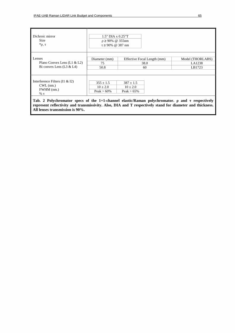
IFAE-UAB Raman LIDAR Link Budget and Components 65
Dichroic mirror
Size *ρ, τ
1.5" DIA x 0.25"T ρ ≥ 90% @ 355nm τ ≥ 90% @ 387 nm
Lenses
Plano Convex Lens (L1 & L2) Bi convex Lens (L3 & L4)
Diameter (mm) Effective Focal Length (mm) Model (THORLABS) 75 38.0 LA1238
50.8 60 LB1723
Interference Filters (I1 & I2)
CWL (nm.) FWHM (nm.) % τ
355 ± 1.5 387 ± 1.5 10 ± 2.0 10 ± 2.0
Peak > 60% Peak > 65%
Tab. 2 Polychromator specs of the 1+1-channel elastic/Raman polychromator. ρ and τ respectively represent reflectivity and transmissivity. Also, DIA and T respectively stand for diameter and thickness. All lenses transmission is 90%.