master thesis sheet metal forming simulations with fem
TRANSCRIPT

Master Thesis
Sheet metal forming simulations withFEM
Filip Lindberg
January 24, 2012

Sheet Metal Forming Simulations with FEM
Master’s Thesis in Engineering Physics, 30 ECTS
Filip Lindberg
Department of Physics
Master of Science Programme in Engineering Physics
Umeå University
SE-901 87 Umeå, Sweden
Author: FILIP LINDBERG, Umeå University. Tel: +46 (0)70-660 21 93
Supervisor: ERIK LINDBERG, Duroc Tooling in Robertsfors. Tel: +46 (0)70-595 52 05
Examiner: CLAUDE LACOURSIÈRE, Umeå University. Tel: +46 +46 (0)70-675 42 42

Abstract
The design of new forming tools get more problemtic as the geometries get more complicated
and the materials less formable. The idea with this project is to evaluate if an implementation
of a simulation software in the designing process, to simulate the forming process before
actually building the tools, could help Duroc Tooling avoid expensive mistakes. To evaluate
this, the commercial FEM simulation software LS-DYNA was used in a complicated project,
where the design of the forming tools for forming a girder was considered. The main objective
was to avoid cracking and severe wrinkling which may result in the forming process.
With help of simulations a stable forming process which did not yield cracks or severe
wrinkling, was eventually found. The girder was almost impossible to form without cracking,
but the breakthrough came when we tried to simulate a preforming step which solved the
problem. Without a simulation software this would never have been tested since it would be
to risky and expensive to try an idea which could turn out to be of no use. The simulations
also showed that the springback - shape deformation occuring after pressing - was large
and hard to predict without simulations. Therefore, the tools were also finally springback
compensated.
We concluded that simulations are very effective to quickly test new ideas which may be
necessary when designing the tools for forming complicated parts. Simulation also provided
detailed quantitative information about the expected cracks, wrinkles, and weaknesses of the
resulting pieces. Even though there is cost associated with simulations, it is obvious from this
project that a simulation software is a must if Duroc Tooling wants to be a leading company
in sheet metal forming tools, and stand ready for the higher demands on the products in the
future.

Sammanfattning
Konstruktionerna av nya formningsverktyg blir allt mer problematiska allteftersom geome-
trierna blir mer komplicerade och materialen mindre formbara. Tanken med detta projekt
är att utvärdera hur om en implementation av ett simuleringsverktyg under konstruktion-
sprocessen, för att simulera formningsprocessen innan man faktiskt bygger verktygen, skulle
kunna hjälpa Duroc Tooling att undvika dyra misstag. För att utvärdera detta användes det
kommersiella FEM-simuleringsprogrammet LS-DYNA i ett svårt projekt där konstruktionen
av formningsverktygen, för att pressa en balk, skulle tas fram. Huvudmålet var att undvika
sprickbildning och skrynkelbildning som kan bli ett resultat efter en formning.
Med häjlp av simuleringar hittades till slut en stabil formningsprocess som inte gav sprickor
eller allvarlig skrynkelbildning. Balken var nästan omöjlig att forma utan sprickor, men
genombrottet kom när vi testade att simulera ett förformningssteg vilket löste problemet.
Utan ett simuleringsverktyg skulle aldrig detta blivit testat eftersom att det skulle vara
alldeles för riskabelt och dyrt att testa en idé som sedan kanske skulle kunna visa sig vara
utan nytta. Simuleringarna visade också att återfjädringen - deformationen efter pressningen
- var relativt stor och svår att förutse utan simuleringar. Därför återfjädringskompenserades
verktygen slutligen.
Vi drog slutsaten att simuleringar är väldigt effektiva för att snabbt testa nya ideér som
kan vara nödvändiga när man konstruerar verktyg för komplicerade detaljer. Simuleringarna
gav även detaljerad kvantitativ information om sprickor, skrynkelbildning och svagheter av
den slutgiltiga detaljen. Även fast det finns en viss kostnad associerad med simuleringar så
är det uppenbart från studien att simuleringar är ett måste om Duroc Tooling will fortsätta
vara ett ledande företag inom metallformningsverktyg och stå redo för de högre kraven på
produkterna i framtiden.
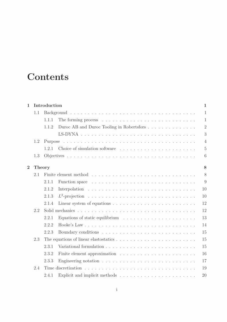
Contents
1 Introduction 1
1.1 Background . . . . . . . . . . . . . . . . . . . . . . . . . . . . . . . . . . . . 1
1.1.1 The forming process . . . . . . . . . . . . . . . . . . . . . . . . . . . 1
1.1.2 Duroc AB and Duroc Tooling in Robertsfors . . . . . . . . . . . . . . 2
LS-DYNA . . . . . . . . . . . . . . . . . . . . . . . . . . . . . . . . . 3
1.2 Purpose . . . . . . . . . . . . . . . . . . . . . . . . . . . . . . . . . . . . . . 4
1.2.1 Choice of simulation software . . . . . . . . . . . . . . . . . . . . . . 5
1.3 Objectives . . . . . . . . . . . . . . . . . . . . . . . . . . . . . . . . . . . . . 6
2 Theory 8
2.1 Finite element method . . . . . . . . . . . . . . . . . . . . . . . . . . . . . . 8
2.1.1 Function space . . . . . . . . . . . . . . . . . . . . . . . . . . . . . . 9
2.1.2 Interpolation . . . . . . . . . . . . . . . . . . . . . . . . . . . . . . . 10
2.1.3 L2-projection . . . . . . . . . . . . . . . . . . . . . . . . . . . . . . . 10
2.1.4 Linear system of equations . . . . . . . . . . . . . . . . . . . . . . . . 12
2.2 Solid mechanics . . . . . . . . . . . . . . . . . . . . . . . . . . . . . . . . . . 12
2.2.1 Equations of static equilibrium . . . . . . . . . . . . . . . . . . . . . 13
2.2.2 Hooke’s Law . . . . . . . . . . . . . . . . . . . . . . . . . . . . . . . . 14
2.2.3 Boundary conditions . . . . . . . . . . . . . . . . . . . . . . . . . . . 15
2.3 The equations of linear elastostatics . . . . . . . . . . . . . . . . . . . . . . . 15
2.3.1 Variational formulation . . . . . . . . . . . . . . . . . . . . . . . . . . 15
2.3.2 Finite element approximation . . . . . . . . . . . . . . . . . . . . . . 16
2.3.3 Engineering notation . . . . . . . . . . . . . . . . . . . . . . . . . . . 17
2.4 Time discretization . . . . . . . . . . . . . . . . . . . . . . . . . . . . . . . . 19
2.4.1 Explicit and implicit methods . . . . . . . . . . . . . . . . . . . . . . 20
i

Umeå UniversityMaster’s Thesis, 30 ECTSSheet Metal Forming Simulations with FEM
Filip LindbergJanuary 24, 2012
Robertsfors
Stability and numerical accuracy . . . . . . . . . . . . . . . . . . . . 20
2.5 Material properties . . . . . . . . . . . . . . . . . . . . . . . . . . . . . . . . 21
2.5.1 Anisotropy . . . . . . . . . . . . . . . . . . . . . . . . . . . . . . . . . 23
2.5.2 Rate sensitivity . . . . . . . . . . . . . . . . . . . . . . . . . . . . . . 24
2.6 Strains, incompressibility condition and general sheet processes . . . . . . . . 24
2.7 Tresca and Von Mises yield criterions . . . . . . . . . . . . . . . . . . . . . . 25
2.8 Effective stress and strain . . . . . . . . . . . . . . . . . . . . . . . . . . . . 26
2.9 Instability and tearing . . . . . . . . . . . . . . . . . . . . . . . . . . . . . . 27
2.9.1 Forming limit diagram . . . . . . . . . . . . . . . . . . . . . . . . . . 28
2.9.2 The forming window . . . . . . . . . . . . . . . . . . . . . . . . . . . 30
2.10 LS-DYNA . . . . . . . . . . . . . . . . . . . . . . . . . . . . . . . . . . . . . 31
2.10.1 Contacts . . . . . . . . . . . . . . . . . . . . . . . . . . . . . . . . . . 31
3 Method 34
3.1 Stages . . . . . . . . . . . . . . . . . . . . . . . . . . . . . . . . . . . . . . . 34
3.2 Methodology . . . . . . . . . . . . . . . . . . . . . . . . . . . . . . . . . . . 34
3.3 Setting up a simulation . . . . . . . . . . . . . . . . . . . . . . . . . . . . . . 35
3.3.1 Preprocessing . . . . . . . . . . . . . . . . . . . . . . . . . . . . . . . 36
Import the CAD-geometry . . . . . . . . . . . . . . . . . . . . . . . . 36
Create the blank . . . . . . . . . . . . . . . . . . . . . . . . . . . . . 38
Tool Meshing . . . . . . . . . . . . . . . . . . . . . . . . . . . . . . . 38
Part Meshing . . . . . . . . . . . . . . . . . . . . . . . . . . . . . . . 40
Materials . . . . . . . . . . . . . . . . . . . . . . . . . . . . . . . . . 42
Position tools and set up tool motions . . . . . . . . . . . . . . . . . 44
Set up the controls for adaptive refinements . . . . . . . . . . . . . . 45
3.3.2 Executing the simulation . . . . . . . . . . . . . . . . . . . . . . . . . 48
Run the simulation . . . . . . . . . . . . . . . . . . . . . . . . . . . . 49
Setup springback simulation . . . . . . . . . . . . . . . . . . . . . . . 50
Run the springback simulation . . . . . . . . . . . . . . . . . . . . . . 52
3.3.3 Postprocessing . . . . . . . . . . . . . . . . . . . . . . . . . . . . . . 53
Evaluate simulation results . . . . . . . . . . . . . . . . . . . . . . . . 53
Springback compensation . . . . . . . . . . . . . . . . . . . . . . . . 56
Duroc Tooling ii

Umeå UniversityMaster’s Thesis, 30 ECTSSheet Metal Forming Simulations with FEM
Filip LindbergJanuary 24, 2012
Robertsfors
4 Results 58
4.1 Forming approaches . . . . . . . . . . . . . . . . . . . . . . . . . . . . . . . . 58
4.1.1 First approach . . . . . . . . . . . . . . . . . . . . . . . . . . . . . . 59
4.1.2 Second approach . . . . . . . . . . . . . . . . . . . . . . . . . . . . . 59
Blank shape modifications . . . . . . . . . . . . . . . . . . . . . . . . 70
4.1.3 Third Approach . . . . . . . . . . . . . . . . . . . . . . . . . . . . . . 72
4.1.4 Fourth Approach . . . . . . . . . . . . . . . . . . . . . . . . . . . . . 75
4.2 Springback compensation . . . . . . . . . . . . . . . . . . . . . . . . . . . . . 79
4.3 Blank Shape . . . . . . . . . . . . . . . . . . . . . . . . . . . . . . . . . . . . 81
4.4 Final results . . . . . . . . . . . . . . . . . . . . . . . . . . . . . . . . . . . . 81
5 Discussion 83
5.1 Simulation software . . . . . . . . . . . . . . . . . . . . . . . . . . . . . . . . 83
5.1.1 Reliability and robustness . . . . . . . . . . . . . . . . . . . . . . . . 83
5.1.2 Efficiency . . . . . . . . . . . . . . . . . . . . . . . . . . . . . . . . . 85
5.1.3 Profits and costs . . . . . . . . . . . . . . . . . . . . . . . . . . . . . 87
5.1.4 Future . . . . . . . . . . . . . . . . . . . . . . . . . . . . . . . . . . . 89
5.2 The girder . . . . . . . . . . . . . . . . . . . . . . . . . . . . . . . . . . . . . 89
5.2.1 Optimization and time . . . . . . . . . . . . . . . . . . . . . . . . . . 90
5.3 Main conclusions . . . . . . . . . . . . . . . . . . . . . . . . . . . . . . . . . 91
5.4 Further work . . . . . . . . . . . . . . . . . . . . . . . . . . . . . . . . . . . 92
Bibliography 92
Duroc Tooling iii

Chapter 1
Introduction
1.1 Background
In this section a short introduction to the stamping and forming process will be given.
1.1.1 The forming process
Sheet metal forming, or stamping, is a process where a material, referred to as the blank, is
formed by stretching it between a punch and a die, see figure (1.1). First, the punch and the
binder or blank-holder is in an uplifted position. The binder then moves down and clamps
the blank in such a way that the blank is allowed to be drawn inwards, but still creates
tension to stretch the blank between the die and the punch. In some cases, draw-beads are
also used to further increase the resistance of inwards drawing. After this, the punch moves
down and the sheet is drawn through the opening of the die ring.
1

Umeå UniversityMaster’s Thesis, 30 ECTSSheet Metal Forming Simulations with FEM
Filip LindbergJanuary 24, 2012
Robertsfors
Figure 1.1: (a) Part formed in a stamping process. (b) Overview of the assembly showing the binder, punch
and die.
(Z. Marciniak, Mechanics of Sheet Metal Forming, Butterworth-Heinemann 2002)
Note that the forming process not is a compression process, but rather a stretching pro-
cess, i.e. the blank is stretched over the tools. Since the blank, for the most part, only is
in contact with the tooling on one side, no through-thickness compression is present. The
flow stress in the sheet is generally much larger than the contact pressure, and thus, it is as-
sumed that there is no through-thickness compression. This is called plane stress deformation
[Marciniak(2002)].
Stamping or forming can be done in a single- or double-acting press. A double-acting press
is a press in which the clamping and punch actions are seperate. Usually the forming has to
be done in several stages, different presses, if the desired geometry is complex.
1.1.2 Duroc AB and Duroc Tooling in Robertsfors
Duroc’s activity began in the 1980th as a collaboration with Luleå University in an attempt
to refine metallic surfaces, using laser treatments. The current company was founded 1993.
Duroc posseses unique competence in laser based surface refinements, which also serves as
the base for the work at Duroc Engineering, Duroc Tooling in Olofström and Duroc Welding.
Duroc is listed on the swedish stock exchange NASDAQ OMX Stockholm. The corporate
group turns over 500 Mkr annually and have approximately 200 co-workers.
Duroc Tooling in Robertsfors is a subsidiary company of Duroc AB, which offers develop-
ment, design and production of stamping- and cutting tools, fixtures and components for the
Duroc Tooling 2

Umeå UniversityMaster’s Thesis, 30 ECTSSheet Metal Forming Simulations with FEM
Filip LindbergJanuary 24, 2012
Robertsfors
aerospace-, vehicular- and manufacturing industry. The production is usually only one piece,
or sometimes in shorter series, usually together with the customers development department.
Figure 1.2: The logo of the Duroc corporate group
LS-DYNA
LSTC (Livermore Software Technology Corp.), the developers of LS-DYNA, describes the
program in the following sentence:
LS-DYNA is a general purpose transient dynamic finite element program ca-
pable of simulating complex real world problems. [LSTC(2011)]
LS-DYNA is a combined explicit/implicit solver. The program was orginally designed for
highly transient dynamics FEA, using explicit time integration. Transient dynamics, refers to
events with high speed and short duration where inertial forces are important. The implicit
solver was first implemented in 1998 and is still being developed. LS-DYNA is primarily used,
for its fast explicit solver, in nonlinear problems with large deformations, such as, predicting
a car’s behavior in a collision. The following analysis capabilities are availiable in LS-DYNA
[FEA-information Inc.(2009)]:
• Nonlinear dynamics
• Rigid body dynamics
• Quasi-static simulations
• Normal modes
• Linear statics
• Fluid analysis
• FEM-rigid multi-body dynamics coupling
• Underwater shock
• Failure analysis
Duroc Tooling 3

Umeå UniversityMaster’s Thesis, 30 ECTSSheet Metal Forming Simulations with FEM
Filip LindbergJanuary 24, 2012
Robertsfors
• Crack propagation
• Real-time acoustics
• Design optimization
• Implicit springback
• Multi-physics coupling
• Structural-thermal coupling
• Adaptive Remeshing
1.2 Purpose
The production of new stamping tools get more troublesome, as the geometries get more
complex and smaller tolerances on the dimensions are requested. This increases the risk
for unexpected scenarios that could compromise the entire project. Thus, to deal with this,
Duroc wants to try a more advanced simulation tool, than the one-step solver they already
have, to investigate what it could mean for future development of the company.
To investigate this, Duroc wants to use a simulation program in a real project to see its
benefits at work and then evaluate if investment in a simulation tool and in personal would
be profitable.
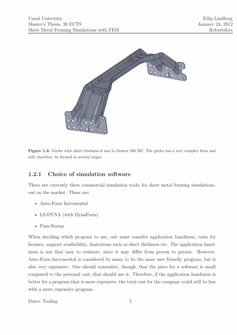
In this project the design of stamping tools, for stamping a girder, placed in a truck, will
be considered, see figure (1.3). Note that the geometry is very complex and stamping in a
single forming step is not possible but several stages will be necessary to form the part.
Duroc Tooling 4
Umeå UniversityMaster’s Thesis, 30 ECTSSheet Metal Forming Simulations with FEM
Filip LindbergJanuary 24, 2012
Robertsfors
Figure 1.3: Girder with sheet thickness 6 mm in Domex 500 MC. The girder has a very complex form and
will, therefore, be formed in several stages
1.2.1 Choice of simulation software
There are currently three commercial simulation tools, for sheet metal forming simulations,
out on the market. These are:
• Auto-Form Incremental
• LS-DYNA (with DynaForm)
• Pam-Stamp
When deciding which program to use, one must consider application handiness, costs for
licenses, support availiability, limitations such as sheet thickness etc. The application hand-
iness is not that easy to evaluate, since it may differ from person to person. However,
Auto-Form Incremental is considered by many to be the most user friendly program, but is
also very expensive. One should remember, though, that the price for a software is small
compared to the personal cost, that should use it. Therefore, if the application handiness is
better for a program that is more expensive, the total cost for the company could still be less
with a more expensive program.
Duroc Tooling 5

Umeå UniversityMaster’s Thesis, 30 ECTSSheet Metal Forming Simulations with FEM
Filip LindbergJanuary 24, 2012
Robertsfors
When it comes to limitations, Autoform Incremental does not handle thick metal sheets,
hydroforming and hot-forming. To handle this, one needs to buy extra softwares such as
Stampack. This is a major drawback since Duroc Tooling sometimes works with thick sheet
metals as well as hot forming. LS-DYNA, on the other hand, has all these features built
in, but the free pre-processor, LS-PrePost, that comes with LS-DYNA, has some drawbacks,
especially when it comes to meshing. To optimally use LS-DYNA, one should also probably
use it together with a pre-processor such as DynaForm. Also, DynaForm has built in a
function to springback compensate the tools which could be very useful.
A big advantage with LS-DYNA is the availability of free support, in swedish, from the
resellers at DynaMore in Linköping. Autoform does not have any swedish telephone support
and the same goes for Pam-Stamp.
Also looking at which software many of the large swedish companies use, one finds LS-
DYNA to be very popular. This goes for Volvo Car Corporation, Scania, Saab Automobile
and many more. [DynaMore Nordic(2011)] Also one of Duroc Tooling’s competitors, Lidhs,
uses LS-DYNA. [Lidhs(2010)]
Primarily because of the limitations in Autoform Incremental, I think that LS-DYNA, to-
gether with the preprocessor DynaForm, will meet the needs best for Duroc Tooling. It
should be mentioned, though, that the decision of software is not that easy, or objective,
since there are very few comparisons availiable. Thus one should try out all the softwares
to really make a fair decision. The most important thing, however, is that the program can
handle the problems in interest and give accurate results. Nevertheless I together with my
supervisor decided to go on and test LS-DYNA.
1.3 Objectives
The main part of this project lies in simulating the different stages of the stamping process
and together with a design engineer decide how the forming tools should be designed. This
will, hopefully, make the design process more smooth and also spare the company expensive
trial and error time. Also, after the project the company can, at least, qualitatively evaluate
if an advanced simulation tool would be profitable for Duroc Tooling. The evaluation of the
simulation tool is also the main purpose for this project. The objectives for this thesis can
be summed up in the following list:
Duroc Tooling 6

Umeå UniversityMaster’s Thesis, 30 ECTSSheet Metal Forming Simulations with FEM
Filip LindbergJanuary 24, 2012
Robertsfors
• Setup a simulation for each stage of the forming process.
• At each stage, evaluate the results of simulations and propose design changes to avoid
cracks, wrinkles, or other unwanted deformations if present.
• Make simulations to find a good blank shape
• Simulate springback after the last stage and compensate the tools for the springback.
• Make a return on invesetment (ROI) calculation, to evaluate the profits that could be
made by implementing a simulation tool in the design process.
Duroc Tooling 7

Chapter 2
Theory
In this chapter the underlying theory, for the applications, will be described. The purpose of
this chapter is to get the reader familiar with the finite element method and the governing
equations as well as some theory for materials and the tools to anaylze the results of the
sheet metal forming process.
2.1 Finite element method
When dealing with computational modelling of a physical process, there are three important
steps to be adressed:
• problem definition
• mathematical model
• computer simulation
In the first step, one first defines the problem to obtain a well-posed problem, i.e. such
that the problem has a unique solution for a given set of parameters. Secondly, the defined
problem should be represented by a mathematical model, such as Navier-Stokes equations in
the case of fluid dynamics. Finally, having chosen the appropriate model with boundary and
initial conditions, the numerical solution of the problem should be obtained. Three common
choices are available, the finite difference method (FDM), the finite element method, FEM,
and the finite volume method, FVM [Peir´o and Sherwin(2005)]. In this project, the finite
element method will be used.
8

Umeå UniversityMaster’s Thesis, 30 ECTSSheet Metal Forming Simulations with FEM
Filip LindbergJanuary 24, 2012
Robertsfors
The finite element method is a numerical technique used for approximating solutions to
partial differential equations, PDEs. The technique is very powerful when solving PDEs over
complicated geometries, domains that changes over time, irregular domains or when the pre-
cision is more important on some areas of the domain. This is in contrast with FDM, which
uses a topologically square network of lines to discretize the domain. Therefore, complex
geometries are hard to handle with FDM.
Although the FEM-method is a purely mathematical concept, it has many applications
on physical problems such as to predict the deformation and stress fields within solid bodies
subjected to external forces. The area of FEM application is usually referred to as finite
element analysis, FEA. Some parts of the theory will be studied in 1D for simplification.
Note, however, that the applications are usually 2D or 3D. Most parts of the theory of the
finite element method will be taken from [Larson and Bengzon(2010)].
2.1.1 Function space
Let I = [a, b] be an one-dimensional interval divided into N subintervals by N + 1 nodes
denoted by xiNi=0. The subintervals will be denoted Ii = [xi−1, xi], for i = 1, 2, ..., N and
have a length hi = xi − xi−1. This partition is called the mesh of the domain. Introduce the
function space Vh of continous piecewise linear functions over the interval I as
Vh = v : v ∈ C(I), v|Ii∈ P1(Ii) (2.1)
with the space C(I) of continuous functions on I and the space P1(Ii) of linear functions on
Ii. The functions in Vh, thus, become linear on each subinterval Ii and continous on I.
Thus any function in Vh will be determined from its nodal values. One can also note that
for each set of nodal values in the interval I one can find a function with these nodal values.
Based on this insight we introduce a basis ϕjNj=0 ⊂ Vh, also known as hat functions, where
ϕj(xi) =
1 if i = j
0 if i 6= j, for i, j = 0, 1, ..., N (2.2)
The hat functions is thus continuous piecewise linear and zero at all nodes except at its
corresponding node xi where it equals one, see figure (2.1). Note the characteristic peaked
shape of the hat functions. Also note that ϕ0 and ϕN have a different shape, half hat, since
Duroc Tooling 9

Umeå UniversityMaster’s Thesis, 30 ECTSSheet Metal Forming Simulations with FEM
Filip LindbergJanuary 24, 2012
Robertsfors
they are located at the boundaries of the interval. With this basis, all functions v ∈ Vh could
be written as a linear combination of the hat functions
v(x) =N∑
i=0
aiϕi(x) (2.3)
where ai is the nodal value of the function v.
Figure 2.1: The basis functions ϕ0 and ϕ1. Note also the "half-hat" shape of ϕ0.
2.1.2 Interpolation
We are now inerested in constructing approximations to a given function f . The easiest
one is called linear interpolation. The definition of the linear interpolation of a continuous
function f is
πf = f(x0)ϕ0 + f(x1)ϕ1 (2.4)
where the interpolation πf and the function f are equal at the the nodes but not necessarily
elsewhere. For the case of continous piecewise linear functions the interpolant is defined as
πf =N∑
i=0
f(xi)ϕi (2.5)
2.1.3 L2-projection
We will now look at another way of approximating a continuous function. The interpolation
approximates the function exactly at the nodes but the L2-projection gives an approximation
that is more accurate on the average, but not exactly on the nodes.
Duroc Tooling 10

Umeå UniversityMaster’s Thesis, 30 ECTSSheet Metal Forming Simulations with FEM
Filip LindbergJanuary 24, 2012
Robertsfors
The definition of the L2-projection reads as follows. Given a function f ∈ L2(I) the
L2-projection Phf ∈ Vh is∫
I(f − Phf)vdx = 0, ∀v ∈ Vh (2.6)
To understand what this means, we start by defining the space L2(I) of square integrable
functions over the interval I as
L2(I) = v :∫
Iv2dx < ∞ (2.7)
with the corresponding scalar product
(v, w) =∫
Ivwdx, ∀v, w ∈ L2 (2.8)
The L2-norm will then be defined as
‖v‖L2 =√
(v, v) =
√
∫
Iv2dx (2.9)
Two functions are orthogonal to each other if the scalar product (v, w) = 0.
If we now turn back to equation (2.6), one notices that this equation defines an orthogonal
projection Phf of f onto the space Vh, i.e. the difference f − Phf is orthogonal to all
functions of v in Vh. The difference between the linear interpolation and the L2-projection,
for f(x) = cos2(x), can be seen in figure (2.2).
Figure 2.2: Different approximaton methods for f(x) = cos2(x).
Duroc Tooling 11

Umeå UniversityMaster’s Thesis, 30 ECTSSheet Metal Forming Simulations with FEM
Filip LindbergJanuary 24, 2012
Robertsfors
2.1.4 Linear system of equations
For a function v(x) =∑N
i=0 aiϕi(x) we note that equation (2.6) can be written∫
I(f − Phf)ϕidx = 0, i = 0, 1, ..., N (2.10)
this may be understand by noting that equation (2.6) is satisfied for every choice of v ∈ Vh
and thus the equation will also be satisfied for any linear combination of functions.
The L2-projection Phf can now be written as a linear combination of hat functions since
Ph ∈ Vh, i.e.
Phf =N∑
j=0
ξjϕj (2.11)
Using this, equation (2.6) can now, after some rearrangement, be written
∫
Ifϕidx =
N∑
j=0
ξj
∫
Iϕjϕidx, i = 0, 1, ..., N (2.12)
To simplify, set
mij =∫
Iϕjϕidx, for i, j = 0, 1, ..., N (2.13)
bi =∫
Ifϕidx, for i = 0, 1, ..., N (2.14)
which then gives
bi =N∑
j=0
mijξj , for i = 0, 1, ..., N (2.15)
This is a linear system of equations with the unknown coefficients ξj. This system of equations
can be written in matrix form
Mξ = b (2.16)
We will refer to the matrix, M , as the mass matrix and the vector, b, as the load vector. The
unknown coefficients, ξj, and the orthogonal projection can then be calculated from linear
algebra as
ξ = M−1b (2.17)
2.2 Solid mechanics
In this section solid mechanics, which is one of the most important areas of application of
the finite element method, will be studied. The main objective is to predict the deformation
and stress fields within solid bodies subjected to external forces.
Duroc Tooling 12

Umeå UniversityMaster’s Thesis, 30 ECTSSheet Metal Forming Simulations with FEM
Filip LindbergJanuary 24, 2012
Robertsfors
2.2.1 Equations of static equilibrium
In equilibrium the net force acting on a solid body must vanish. For a volume there are two
kinds of forces of concern. The first one are forces that penetrates the whole volume, such
as gravity. This force can be described as a force density f . Then there are also contact
forces which act on the surface of the volume. Contact forces are described by vector fields
that exists through the whole volume even though it is only in contact with the surface. The
contact forces will be described by the stress tensor σ. This tensor is a 3x3 matrix defined
such that the component σi,j is the force per unit area acting in the direction xi on a surface
with the normal in the direction of xj . The total force acting on a volume V will thus be a
sum of both contact and volume forces
F =∫
VfdV +
∫
Sσ · ndS (2.18)
Using the divergence theorem on the surface integral the following expression for the total
force is obtained
F =∫
V(f + ∇ · σ)dV (2.19)
where
(∇ · σ) =3∑
j=1
∂σij
∂xj, i = 1, 2, 3 (2.20)
In equilibrium the total force F for a solid body should be equal zero. Thus
f + ∇ · σ = 0 (2.21)
This equation is known as Cauchy’s equation of equilibrium and states that the net force of
every particle in a solid vanishes. In component form this equation becomes
f1 +∂σ11
∂x1
+∂σ12
∂x2
+∂σ13
∂x3
= 0 (2.22)
f2 +∂σ21
∂x1
+∂σ22
∂x2
+∂σ23
∂x3
= 0 (2.23)
f3 +∂σ31
∂x1
+∂σ32
∂x2
+∂σ33
∂x3
= 0 (2.24)
One also needs constitutive equations that expresses the local relations between the stresses
and the local state of matter. If conservation of angular momentum is enforced it can be
shown that the stress tensor must be symmetric, i.e.
σ = σT (2.25)
which eliminates three independent components in the stress tensor.
Duroc Tooling 13

Umeå UniversityMaster’s Thesis, 30 ECTSSheet Metal Forming Simulations with FEM
Filip LindbergJanuary 24, 2012
Robertsfors
2.2.2 Hooke’s Law
The deformation of a solid may be described by the particles displacements from their initial
position. The displacement vector is defined as u = r − r0 where r is the current position
and r0 is the initial position for the particle. The deformation of the body is described with
the strain tensor, which for small displacements can be defined as
ǫ =12
(∇u + ∇uT ) (2.26)
A deformation of a solid is caused by a displacement u and thus the strain tensor is
nonzero, i.e. ǫ 6= 0. Note that for rigid body translations and rotations the stress tensor is
in fact zero since there is no deformation. Thus local stresses only depend on local strains.
Hooke’s law which is a consitutive law states that for small strains, the relationship between
the stress tensor and the strain tensor is approximately linear. Now, assume an isotropic
material, i.e. a material where the properties are independent of spatial direction. Also
assume that, initially, there are no stresses. By symmetry reasons the following relationship
is obtained
σ = 2µǫ(u) + λ(∇ · u)I (2.27)
The elastic moduli µ and λ are defined by
µ =E
2(1 + ν)(2.28)
λ =Eν
(1 + ν)(1 − 2ν)(2.29)
where E is Young’s elastic modulus which is a material parameter that defines the stiffnes of
the material and ν, Poisson’s ratio, which is a material parameter that gives a relationship
between the strain in the tensile direction and the strain in the transverse direction. Equation
(2.21) and equation (2.27) now gives the governing equations for the displacement u
−∇ · σ = f (2.30a)
σ = 2µǫ(u) + λ(∇ · u)I (2.30b)
Duroc Tooling 14

Umeå UniversityMaster’s Thesis, 30 ECTSSheet Metal Forming Simulations with FEM
Filip LindbergJanuary 24, 2012
Robertsfors
2.2.3 Boundary conditions
The boundary conditions are essential to obtain useful results. There are two kinds of bound-
ary conditions. One of them is the Dirichlet and the other is the Neumann boundary con-
dition. The Dirichlet boundary condition controls the displacement, u, and is given on the
form u = gD, where gD is a given function. Neumann boundary conditions on the other
hand set constraints on the nomal stress and is thus given on the form σ · n = gN .
2.3 The equations of linear elastostatics
We will now turn to the problem of finding the stress tensor σ and the displacement vector
u on a domain Ω. Assume that the domain is occupied by a homogeneous isotropic linear
elastic solid, the problem then reads
−∇ · σ = f , in Ω (2.31a)
σ = 2µǫ(u) + λ(∇ · u)I, in Ω (2.31b)
u = gD, on ΓD (2.31c)
σ · n = gN , on ΓN (2.31d)
where ΓD and ΓN are the boundary segments of the domain.
2.3.1 Variational formulation
To solve this problem, the first step is to make a variational formulation of the problem.
Begin by choosing a trial space
V = v ∈ [H1(Ω)]3 (2.32)
where H1 is the Hilbert space defined as
H1 = v : ‖∇v‖ + ‖v| < ∞ (2.33)
The next step is to multiply equation −∇ · σ = f with a test function v ∈ V and then
Duroc Tooling 15

Umeå UniversityMaster’s Thesis, 30 ECTSSheet Metal Forming Simulations with FEM
Filip LindbergJanuary 24, 2012
Robertsfors
integrating by parts
−(∇ · σ, v) =3∑
i,j=1
(−∂σij
∂xj, vi) (2.34)
=3∑
i,j=1
−(σij , njvi)∂Ω + (σij ,∂vi
∂xj
) (2.35)
= (f, v) (2.36)
This equation can be rewritten as
−(σ · n, v)∂Ω + (σ : ∇v) = (f, v) (2.37)
where the operator : has the following definition
A : B =3∑
i,j=1
AijBij (2.38)
The variational formulation now reads:
Find u ∈ V such that
(σ : ∇v) − (σ · n, v)∂Ω = (f, v) (2.39)
Further, recalling that σ is symmetric, we get
σ : ∇v =12
(∇v + ∇vT ) +12
(∇v − ∇vT ) = σ : ǫ(v) + 0 (2.40)
Now using this in equation (2.39), the following equation is obtained
(σ(u) : ǫ(v))Ω = (f, v) + (σ · n, v)∂Ω (2.41)
Insert σ = 2µǫ(u) + λ(∇ · u)I in equation (2.41). The variational formulation finally reads:
Find u ∈ V such that∫
Ω
2µǫ(u) : ǫ(v) + λ(∇ · u)(∇ · v)dx = (f, v) + (gN , v)∂Ω, ∀v ∈ V (2.42)
2.3.2 Finite element approximation
It can be shown by using the Lax-Milgram lemma that the variational formulation (2.42) has a
unique solution u ∈ V . This can then further be approximated with the finite element method
by first partitioning (meshing) the domain, Ω, into tetrahedrons. Denote the partition by K.
Now introduce the discrete space
Vh = v ∈ [Vh]3 (2.43)
Duroc Tooling 16

Umeå UniversityMaster’s Thesis, 30 ECTSSheet Metal Forming Simulations with FEM
Filip LindbergJanuary 24, 2012
Robertsfors
of all continuous piecewise linears on K with the basis functions ϕiN1 .
The finite element formulation then says: Find uh ∈ Vh, such that∫
Ω
2µǫ(uh) : ǫ(vh) + λ(∇ · uh)(∇ · v)dx = (f, v) + (gN , v)∂Ω, ∀v ∈ Vh (2.44)
2.3.3 Engineering notation
We will now take a look at the engineering notation for the finite element approximation of
the equations of linear elastostatics. First the independent components in the stress vector
is rearranged
σ =[
σ11 σ22 σ33 σ12 σ23 σ31
]T(2.45)
ǫ =[
ǫ11 ǫ22 ǫ33 ǫ12 ǫ23 ǫ31
]T(2.46)
Hooke’s law in equation (2.27) now reads
σ = Dǫ (2.47)
where
D =
λ + 2µ λ λ 0 0 0
λ λ + 2µ λ 0 0 0
λ λ λ + 2µ 0 0 0
0 0 0 µ 0 0
0 0 0 0 µ 0
0 0 0 0 0 µ
(2.48)
Looking at equation (2.42) and rewriting using the fact that
ǫ : σ = ǫT σ = ǫT Dǫ (2.49)
we get∫
Ω
ǫ(v) : σ(u)dx =∫
Ω
ǫT (v)σ(u)dx =∫
Ω
ǫT (v)Dǫ(u)dx (2.50)
Duroc Tooling 17

Umeå UniversityMaster’s Thesis, 30 ECTSSheet Metal Forming Simulations with FEM
Filip LindbergJanuary 24, 2012
Robertsfors
Now use the following ansatz for U ∈ Vh
U =
U1
U2
U3
=
ϕ1 0 0 ϕ2 0 0 · · · ϕN 0 0
0 ϕ1 0 0 ϕ2 0 · · · 0 ϕN 0
0 0 ϕ1 0 0 ϕ2 · · · 0 0 ϕN
d11
d12
d13
d21
d22
d23
...
dN1
dN2
dN3
= ϕd (2.51)
where ϕ contains the hat basis functions and d are the nodal displacements.
Further rewriting equation (2.26) using the engineering notation
ǫ11
ǫ22
ǫ33
2ǫ12
2ǫ23
2ǫ31
=
∂∂x1
0 0
0 ∂∂x2
0
0 0 ∂∂x3
∂∂x2
∂∂x1
0
0 ∂∂x3
∂∂x2
∂∂x3
0 ∂∂x1
u1
u2
u3
(2.52)
To simplify, introduce the strain matrix
B =
∂∂x1
0 0
0 ∂∂x2
0
0 0 ∂∂x3
∂∂x2
∂∂x1
0
0 ∂∂x3
∂∂x2
∂∂x3
0 ∂∂x1
ϕ1 0 0 ϕ2 0 0 · · · ϕN 0 0
0 ϕ1 0 0 ϕ2 0 · · · 0 ϕN 0
0 0 ϕ1 0 0 ϕ2 · · · 0 0 ϕN
(2.53)
The strains and stresses may then be written
ǫ = Bd (2.54)
σ = BDd (2.55)
Duroc Tooling 18

Umeå UniversityMaster’s Thesis, 30 ECTSSheet Metal Forming Simulations with FEM
Filip LindbergJanuary 24, 2012
Robertsfors
The finite element formulation finally reads:
Find U ∈ Vh such that
(∫
Ω
BT DBdx)
d =∫
Ω
ϕT fdx +∫
∂Ω
ϕT gds, ∀v ∈ Vh (2.56)
2.4 Time discretization
When working with a set of equations, that also have a time dependence, one also has to
make a time discretization, such that, 0 = t0 < t1 < t2 < · · · < tL = T , with the time steps
kn = tn − tn−1.
In sheet metal forming processes, we are interested in solving the following equation
KU + CU + MU = F (2.57)
where U are the displacements, K contains the linear elastic forces, C contains the damping
forces and M the inertia forces.
Now discretizing at time tn+1, equation (2.57) will take the following form
Mxn+1 + Cxn+1 + f i(xn+1) = f e(tn+1) (2.58)
where f i are the internal forces and f e are the external forces.
Now, to solve the equation one needs to choose a method of integration. Consider the
following simplified form of equation (2.57)
Mu = f e − f i − fd (2.59)
where fd are the damping forces.
The integration may then be performed, using a step-by-step method, that satisfies the
equation at discrete time intervals, kn, apart.
The time derivates will now be approximated with finite differences by comparing the
displacements at different times. However, choosing at which end-point the quadratures
should be taken, is an important matter, that may give different results. These quadratures
can be separated into explicit and implicit schemes. This will be discussed in the following
section.
Duroc Tooling 19

Umeå UniversityMaster’s Thesis, 30 ECTSSheet Metal Forming Simulations with FEM
Filip LindbergJanuary 24, 2012
Robertsfors
2.4.1 Explicit and implicit methods
A numerical stepping scheme is called explicit when a direct computation of the next, un-
known, time step is made, using only already known quantities from previous time steps.
This is in contrast with the implicit method, which solves the equation by involving the
current state, as well as the later one, which is unknown. Mathematically these stepping
schemes may be written, considering equation (2.59)
U t+∆t = f(U t, U t, U t, U t−∆t, · · · ) Explicit (2.60)
U t+∆t = f(U t+∆t, U t+∆t, U t, · · · ) Implicit (2.61)
It is clear that the implicit method takes more effort to calculate and also may be harder
to implement. When solving with the implicit method, the inversion of the matrix K, in
equation (2.57), is required. Thus, for problems with large deformations, this matrix will be
very large and hence very expensive to compute. However, the implicit method has some
advantages over the explicit. To understand this, we will discuss numerical stability and
numerical accuracy.
Stability and numerical accuracy
As already noted, the explicit method is computaionally fast, but has some problems with
numerical stability. The explicit method is said to be conditionally stable, which means that
the solution will behave bad for too large values of the time step, ∆t. The time step should
be choosen to be less than the critical time step, i.e.
∆t ≤ mine
(
∆xe
ce
)
= mine
∆xe√
Ee
ρe
(2.62)
where ce is the speed of sound in the material, ∆xe the smallest element size in the mesh
[LSTC Inc(2009a)]. Thus, no information can propagate across more than one element for
each time step. LS-DYNA sets the timestep, ∆t = 0.9∆tcritical, to be safe.
The implicit method, on the other hand, can be made unconditionally stable which, in
practise, means that a larger time step can be used. Note, however, that unconditional sta-
bility does not mean that the time step can be chosen arbitrarily large. The time step will
be limited by accuracy considerations. For example, using a too large time step, some high
Duroc Tooling 20

Umeå UniversityMaster’s Thesis, 30 ECTSSheet Metal Forming Simulations with FEM
Filip LindbergJanuary 24, 2012
Robertsfors
frequency content in the solution may be lost. Thus, the implicit solver should be used pri-
marily for problems with low frequency content in which the time dependence of the solution
not is important which, for example, is the case for static and structural problems.
2.5 Material properties
To begin the discussion, let us first, consider the tensile test in which a test-piece is dragged,
see figure (2.3). The piece initially have length l0, width w0 and thickness t0. During the test
the dragging force, P , is measured as well as the extension ∆l = l − l0 and sometimes also
the change in width ∆w = w − w0.
Figure 2.3: An element undergoing a tensile test. During the test the force, P , extension, ∆l and change
in width, ∆w, is measured.
(Z. Marciniak, Mechanics of Sheet Metal Forming, Butterworth-Heinemann 2002)
The relationship between the load and extension can then be plotted in a diagram, see
figure (2.4). At first, the process is elastic, but this part is very small and therefore hard
to see. Eventually, the load reaches Py, the inital yielding load at which plastic deformation
begins. After Py, the deformation in the test-piece is uniform and the load increases. This
is a feature for most metals, in which the hardness of the material increases with plastic
deformation. This phenomena is referred to as strain-hardening. During the whole process,
the cross-sectional area of the piece decreases as the length increases. Eventually, a point is
reached, where the strain-hardening effect and the decrease in cross-section area reaches a
maximum, Pmax. After this, the deformation is not uniform anymore and the deformation
Duroc Tooling 21

Umeå UniversityMaster’s Thesis, 30 ECTSSheet Metal Forming Simulations with FEM
Filip LindbergJanuary 24, 2012
Robertsfors
focuses in the smaller section of the work-piece, i.e. a diffuse neck is created, until the piece
finally fails.
Figure 2.4: The load extension diagram for a test-piece with dimensions l0 = 50, w0 = 12.5, t0 = 0.8 mm.
(Z. Marciniak, Mechanics of Sheet Metal Forming, Butterworth-Heinemann 2002)
Now, one can instead convert this to a stress-strain curve by dividing the load with the
initial cross section area, A0, and the length extension by the inital length, l0. This is
referred to as the engineering stress-strain curve. This curve is widely used but has two
drawbacks. First, the cross-section area decreases during the test and thus the stress will be
underestimated. Second, the strain depends on the initial length of the test-piece and is thus
not a real material property. Instead, the true stress can be used, which is calculated as
σ =P
A(2.63)
where A is the current cross-section area. Further, remember that plastic deformation occurs
at constant volume, i.e.
A0l0 = Al (2.64)
and the true stress can be written
σ =P
A0
l
l0(2.65)
The strain for infinitesimal extensions is given by
dǫ =dl
l(2.66)
Duroc Tooling 22

Umeå UniversityMaster’s Thesis, 30 ECTSSheet Metal Forming Simulations with FEM
Filip LindbergJanuary 24, 2012
Robertsfors
Now, if the straining process continues uniformly, all the contributions should be summed up
ǫ =∫
dǫ =∫ l
l0
dl
l= ln
l
l0(2.67)
A plot of the true stress-strain curve can be seen in figure (2.5) below.
Figure 2.5: The true stress-strain curve for the tensile test.
(Z. Marciniak, Mechanics of Sheet Metal Forming, Butterworth-Heinemann 2002)
A common way to approximate this curve, is by using a simple power-law such as
σ = Kǫn (2.68)
where n is the strain-hardening index and K is the strength-coefficient. This usually works
fine, especially for annealed low carbon steel sheet. [Marciniak(2002)] The description will
be accurate, except for the small elastic part in the beginning of the curve, i.e. for small
strains.
2.5.1 Anisotropy
When the properties in the material does not depend on the direction in which they are
measured, they are called isotropic. However, many materials show different properties de-
pending on the direction they are oriented. For example, in a tensile test, if the strains in
the thickness and width would be different, some sort of anisotropy would be present. This
Duroc Tooling 23

Umeå UniversityMaster’s Thesis, 30 ECTSSheet Metal Forming Simulations with FEM
Filip LindbergJanuary 24, 2012
Robertsfors
material property is measured with the R-value, given as the ratio of width strain, ǫw, to
thickness strain, ǫt, i.e.
R =ǫw
ǫt=
ln(
ww0
)
ln(
t0
t
) (2.69)
Furthermore, using the constant volume assumption
wtl = w0t0l0 (2.70)
The R-value can be rewritten in terms of width and length only
R =ln(
ww0
)
ln(
w0l0wl
) (2.71)
One usually indicates the direction, in which the R-value is measured, by a suffix, i.e. R0,
R45 and R90. If these values are different, the material is said to have planar anisotropy.
This is often described with
∆R =R0 + R90 − 2R45
2(2.72)
and is usually positive for steels, but may take any sign.
When the R-value differs from unity, there is a difference between in-plane and through-
thickness properties, which is commonly described with the normal plastic anisotropy ratio
∆R =R0 + 2R45 + R90
4(2.73)
2.5.2 Rate sensitivity
The strain rate usually have neglectable effects on the material properties. However, if the
speed on the straining process is greatly increased, a small jump in the load-extension diagram
may be seen. This suggests that the material has some strain-rate sensitivity. This can be
mathematically written as
σ = Kǫnǫm (2.74)
2.6 Strains, incompressibility condition and general sheet
processes
Consider a piece of metal with length l0, width w0, and thickness t0, see figure (2.3). Now,
applying a tensile force will alter the length of the piece by dl, width by dw and the thickness
Duroc Tooling 24

Umeå UniversityMaster’s Thesis, 30 ECTSSheet Metal Forming Simulations with FEM
Filip LindbergJanuary 24, 2012
Robertsfors
dt. Let the principal direction along the length of the piece be denoted as 1, along the width,
2, and along the thickness, 3. The principal strain increments can then be written
dǫ1 =dl
l; dǫ2 =
dw
w; dǫ3 =
dt
t(2.75)
It is well known that the volume remains constant during plastic deformation, thus
d(lwt) = d(l0w0t0) = 0 (2.76)
which can be written
dl · wt + dw · lt + dt · lw = 0 (2.77)
and finally dividing by lwt
dl
l+
dw
w+
dt
t= dǫ1 + dǫ2 + dǫ3 = 0 (2.78)
This is called the incompressibility condition.
For a general sheet plane process the following relations hold between the principal stresses
σ1; σ2 = ασ1; σ3 = 0; (2.79)
and for the strains
ǫ1; ǫ2 = βǫ1; ǫ3 = −(1 + β)ǫ1 (2.80)
where α and β are the stress and strain ratios respectively.
2.7 Tresca and Von Mises yield criterions
There are two different theories describing when materials start yielding. The oldest theory
is by Tresca (1864) and suggests that it is the biggest shear stress in the material which
determines when plastic deformation begins. [Dahlberg(2001)] This condition can be written
as the difference between the maximum principal stress and the minimum principal stress
σmax − σmin
2=
σf
2(2.81)
The other theory is by von Mises (1912) which suggests that yielding will commence when
the root-mean-square value of the maximum shear stresses reaches a critical value. This
criteria can be written
σf =
√
1
2(σ1 − σ2)2 + (σ2 − σ3)2 + (σ3 − σ1)2 (2.82)
Duroc Tooling 25

Umeå UniversityMaster’s Thesis, 30 ECTSSheet Metal Forming Simulations with FEM
Filip LindbergJanuary 24, 2012
Robertsfors
where σi, i = 1, 2, 3, are the principal stresses and σf is the flow stress, i.e. the instantaneous
stress requried to continue deform the material. The yield locus for plane stress are plotted
for both Tresca and von Mises in figure (2.6).
Figure 2.6: Yield locus for plane stress for Tresca, blue hexagon, and von Mises, red ellipse.
2.8 Effective stress and strain
Consider a unit cube that undergoes small deformations, such that each side deforms by
1 · dǫ1; 1 · dǫ2 and 1 · dǫ3. The force on each side is σi, i = 1, 2, 3 and thus the work done
during the deformation isdW
vol.= σ1dǫ1 + σ2dǫ2 + σ3dǫ3 (2.83)
The total work during the deformation is
W
vol.=∫ ǫ1
0
σ1dǫ1 +∫ ǫ2
0
σ2dǫ2 +∫ ǫ3
0
σ3dǫ3 (2.84)
We would like to express the work in the form
dW
vol.= f1(σ1, σ2, σ3)df2(ǫ1, ǫ2, ǫ3) (2.85)
Duroc Tooling 26

Umeå UniversityMaster’s Thesis, 30 ECTSSheet Metal Forming Simulations with FEM
Filip LindbergJanuary 24, 2012
Robertsfors
Now since the element is yielding during the deformation, choose the stress function given
by von Mises yield criterion and denote it by σ such that
f1(σ1, σ2, σ3) = σ =
√
1
2(σ1 − σ2)2 + (σ2 − σ3)2 + (σ3 − σ1)2 (2.86)
This function is called the effective or equivalent stress. Henceforth, the strain function
can be found from equation (2.85). This function is called the effective of equivalent strain
increment and can be written
f2(ǫ1, ǫ2, ǫ3) = ǫ =
√
2
9(ǫ1 − ǫ2)2 + (ǫ2 − ǫ3)2 + (ǫ3 − ǫ1)2 (2.87)
The work function will now be given by
dW
vol.=∫ ǫ
0
σǫ (2.88)
Note that the stress function has been chosen as the von Mises and is, thus, equal in magni-
tude to the flow stress when the material is deforming. The effective strain function will also
be equal in magnitude to the strain in uniaxial tension when the same amount of work are
done in the general process and the uniaxial tension. From this, we have found a stress-strain
relation for an isotropic material, undergoing plastic deformation. This relationship is called
the effective stress-strain curve, σ = f(ǫ). [Marciniak(2002), p. 27]
2.9 Instability and tearing
In the sheet metal forming operation, the process may at some time be limited or terminated.
Therefore, trying to predict these process limits are important. All processes have its own
limiting events and are usually one of the following: [Marciniak(2002), p. 61]
• Localized necking or tearing: In the beginning of a tensile deformation the process is
stable and homogenous over the workpiece. However, at some stage, large amounts of
strain might localize in a small region and the local cross-sectional area will decrease.
This is called a neck in the material. If the deformation continues, almost all deforma-
tion will be concentrated in the neck and this instable deformation will eventually lead
to tearing of the material. The reason for necking is due to the fact that all real ma-
terials are imperfect, in the sense that they have small local varaiations in dimensions
and composition, which lead to local fluctuations in stresses and strains.
Duroc Tooling 27

Umeå UniversityMaster’s Thesis, 30 ECTSSheet Metal Forming Simulations with FEM
Filip LindbergJanuary 24, 2012
Robertsfors
• Fracture: In failure analysis, one seperates by ductile failure and brittle failure. Ductile
failure is the same as tearing during localized necking. However, at brittle fracture
the metals experience little or no deformation before fracture and is characterized by
a rapid crack propagation. [Metallurgical Consultants(2010)]
• Wrinkling: This is what might occur if one principal stress is compressive and may
result in wrinkles or buckles in the metal.
2.9.1 Forming limit diagram
The forming limit diagram, FLD, is an analysis tool, for forming processes, that indicates
how close the material is to failure, i.e. necking or fracture. The forming limit curve, FLC,
defines the maximum strain combinations that a metallic sheet can undergo for different
forming conditions, such as deep drawing, stretching, bending and die drawing, without
failure. [ASTM(2012)]
The FLC can be empirically constructed by using a hemispherical punch biaxial stretch
test, as well as a tension test to strain the specimen and then recording the major and
minor strains, ǫ1 and ǫ2 just before necking or before fracture occurs. Note, however, that in
practice there are scatter in the measured strains, just prior to failure, and therefore one do
not consider a single curve but rather a band in which necking or fracture is likely to occur.
[Marciniak(2002), p. 70] An example of a forming limit curve can be seen in figure (2.7)
Figure 2.7: Example of a forming limit curve (FLC) outlining different strain combinations resulting in
failure.
Duroc Tooling 28

Umeå UniversityMaster’s Thesis, 30 ECTSSheet Metal Forming Simulations with FEM
Filip LindbergJanuary 24, 2012
Robertsfors
One way to record the major and minor strains is by covering the surface of the specimen
with a circle and square grid as in figure (2.8). Initially the circles have diameter d0. The
piece is then dragged in biaxial thension. During the deformation the circles will deform
into ellipses with major and minor axes d1 and d2 respectively. Assuming that the square
grid is aligned with the principal directions the deformation will result in a rectangular grid.
[Marciniak(2002), p. 30] Using blanks with different widths, a range of strain states for the
minor direction, ǫ2, can be obtanied. The major strain, ǫ1, is determied by the capacity of
the material to be stretched in one direction at the same time as forces act to either stretch
or compress the specimen in the minor, ǫ2, direction. For example, in the tension test, the
minor strain is negative since the specimen’s thickness and width is narrowed as the piece is
stretched in the major direction.
(a) (b)
Figure 2.8: (a): Circles with diamter d0 in a square grid are marked on the surface. (b) After the deformation
the circles are deformed into elipses with major axis d1 and minor axis d2.
The FLC is material dependent and also depends on the thickness of the sheet, since
thicker specimen have a larger volume to respond to in the forming process. [ASTM(2012)]
Another important property that affects the FLC is the strain hardening exponent, n. For
materials with a higher n value, the limiting major strain will also be higher, see figure (2.9).
Duroc Tooling 29

Umeå UniversityMaster’s Thesis, 30 ECTSSheet Metal Forming Simulations with FEM
Filip LindbergJanuary 24, 2012
Robertsfors
Processes in which biaxial stretching is required to form the part, usually, requires fully
annealed, i.e. high n sheet material. This, however, is a problem since materials with a high
n value normally also have a low initial strength. [Marciniak(2002), p. 75] Also, strengthening
processes, such as cold-working, reduces n and makes forming more difficult.
Figure 2.9: Forming limit curve (FLC) for a high and low n value material respectively.
2.9.2 The forming window
During plastic deformation of metallic materials the volume does not change, i.e. the materi-
als are incompressible and hence one of the principal stresses must be positive. [Anders E W Jarfors(2000)
Considering this, as well as the forming limit curve and the events limiting the forming pro-
cess, it might be useful to construct a forming window in which plane stress sheet forming is
possible. An example of a forming window can be seen in figure (2.10).
Note that the compressive limit is shown at the strain path of β = −2. Since the limit for
wrinkling not solely is a material property, the limit is shown as a region instead. The forming
window should serve as a pictorial aid for forming analysis and not as hard fact, since the
FLC is not only material dependent, but also depends on the thickness of the workpiece and
also the strain path. Remember that materials that has undergone a strengthening process
also have a low n value and thus the forming window gets very narrow. Finding a process to
form strong materials that will permit safe straining in the narrow window is, therefore, one
of the biggest challenges in sheet metal forming.
Duroc Tooling 30

Umeå UniversityMaster’s Thesis, 30 ECTSSheet Metal Forming Simulations with FEM
Filip LindbergJanuary 24, 2012
Robertsfors
Figure 2.10: A forming window showing the limiting events for plane stress deformation.
(Z. Marciniak, Mechanics of Sheet Metal Forming, Butterworth-Heinemann 2002)
2.10 LS-DYNA
In this section we will discuss some theory of some of the implementations in LS-DYNA.
2.10.1 Contacts
When modelling contacts we have two sides of the contact, one master side and one slave
side, see figure (2.11). The contacts are defined by sets (parts, nodes or segments). The
master side is considered as a rigid geometrical surface. Contact occurs when a slave node
penetrates a master segment. The contact is then defined by identifying on what locations
are to be checked for this penetration. [LSTC Inc(2009b)]
Duroc Tooling 31

Umeå UniversityMaster’s Thesis, 30 ECTSSheet Metal Forming Simulations with FEM
Filip LindbergJanuary 24, 2012
Robertsfors
Figure 2.11: The master and the slave side. The program looks for penetration of the slave side through
the master side of the contact.
At every time step, a search for penetration is made. Most of the contacts in LS-DYNA,
at least those recommended, are based on the penalty method. In this method, when a
penetration is found, a force that is proportional to the penetration depth is applied to
eliminate the penetration, see figure (2.12). The default penalty method contact force is
given by
Fi = δik (2.89)
where k is the interface spring stiffness. For shell elements this is given by k = cKAdiagonal
and
for solid elements, k = cKAV/A
, where K is the bulk modulus and c is the penalty factor.
Figure 2.12: The slave side have now penetrated the master side with a distance δi. A force, proportional
to the penetration, will be applied to eliminate the penetration.
Duroc Tooling 32
Umeå UniversityMaster’s Thesis, 30 ECTSSheet Metal Forming Simulations with FEM
Filip LindbergJanuary 24, 2012
Robertsfors
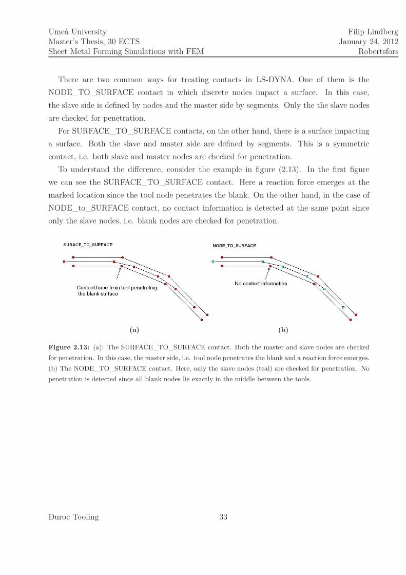
There are two common ways for treating contacts in LS-DYNA. One of them is the
NODE_TO_SURFACE contact in which discrete nodes impact a surface. In this case,
the slave side is defined by nodes and the master side by segments. Only the the slave nodes
are checked for penetration.
For SURFACE_TO_SURFACE contacts, on the other hand, there is a surface impacting
a surface. Both the slave and master side are defined by segments. This is a symmetric
contact, i.e. both slave and master nodes are checked for penetration.
To understand the difference, consider the example in figure (2.13). In the first figure
we can see the SURFACE_TO_SURFACE contact. Here a reaction force emerges at the
marked location since the tool node penetrates the blank. On the other hand, in the case of
NODE_to_SURFACE contact, no contact information is detected at the same point since
only the slave nodes, i.e. blank nodes are checked for penetration.
(a) (b)
Figure 2.13: (a): The SURFACE_TO_SURFACE contact. Both the master and slave nodes are checked
for penetration. In this case, the master side, i.e. tool node penetrates the blank and a reaction force emerges.
(b) The NODE_TO_SURFACE contact. Here, only the slave nodes (teal) are checked for penetration. No
penetration is detected since all blank nodes lie exactly in the middle between the tools.
Duroc Tooling 33

Chapter 3
Method
3.1 Stages
Since the girder has a complicated shape it can not be formed in a single stage. Probably
two or three forming steps will be necessary. First a trimming step to get the right blank
shape is made. After this, two or three forming steps follows, depending on how the tools
will be designed. Finally, a stage where the drilling of the holes is made.
3.2 Methodology
In this section the methodology, for designing a girder, will be described. The design engineer
first proposes a blank shape, this shape might have to be changed gradually as the results
from the simulations are obtained. The design engineer then designs the tool, or the tool
surfaces that are in contact with the blank, for the first forming stage. Since LS-DYNA
will treat the tools as rigid, only the tool surfaces that are in contact with the blank are
required for the simulations. The CAD-model for the tools will then be imported into the
preprocessor DynaForm, where the mesh is generated and the simulation process is set up.
The simulation can then be run in LS-DYNA where output-files are generated. These files
can then be evaluated in LS-PrePost to evaluate strains, displacements and reaction forces.
If the results are acceptable, we are done and the design engineer can go on designing the
second step. Eventually, we might realise that the original blank shape has to be changed.
In that case the simulations must be carried out from the beginning again. The methodology
is schematically described in the scheme in figure (3.1).
34

Umeå UniversityMaster’s Thesis, 30 ECTSSheet Metal Forming Simulations with FEM
Filip LindbergJanuary 24, 2012
Robertsfors
Figure 3.1: Working progress in designing a grider. The design engineer first designs a model for the tool.
The CAD-geometry is imported into Dynaform where the mesh is generated and the forming simulation is
set up. The simulation is then executed in LS-DYNA and the result can then be evaluated in LS-PrePost. If
the result is acceptable we are done, otherwise some design modifications need to be implemeted and then
tested with a new simulation.
3.3 Setting up a simulation
This section will describe the steps for setting up a simulation in DynaForm and LS-DYNA.
The steps in setting up a forming simulations are
• Import the CAD-geometry into DynaForm and check surfaces
• Create the blank or import it from previous forming step
• Mesh the tool surfaces and the blank
• Define material for the blank
• Define the tool motions
• Set up the controls for adaptive refinements, time-step etc.
• Run the simulations, for the trimming and forming steps, in LS-DYNA
• Define constraints for springback simulation in LS-PrePost
Duroc Tooling 35

Umeå UniversityMaster’s Thesis, 30 ECTSSheet Metal Forming Simulations with FEM
Filip LindbergJanuary 24, 2012
Robertsfors
• Simulate the springback
• Evaluate the results in LS-PrePost
This can further be generalised into the following main steps
• Preprocessing
• Executing the simulation
• Postprocessing
which we will discuss more in detail in the following subsections.
3.3.1 Preprocessing
The preprocessing part is where the main part of the work is done. Here the CAD-model
is imported and the simulation is set up. All steps in the preprocessing will be described in
more detail here.
Import the CAD-geometry
The first thing, in the preprocessing part, is to import the CAD-geometries for the tools into
DynaForm. The most common choice is to use the file format IGES, which is designed for
digital exchange of CAD-models between different CAD-systems and is available in most of
the commercial CAD-softwares.
After the model is imported, one has to check that no problems occured during the import.
Sometimes some surface part might go missing, as can be seen in figure (3.2). The missing
surfaces can, however, easily be created in DynaForm to fill the holes.
Duroc Tooling 36

Umeå UniversityMaster’s Thesis, 30 ECTSSheet Metal Forming Simulations with FEM
Filip LindbergJanuary 24, 2012
Robertsfors
Figure 3.2: The figure shows one side of the punch in a forming process. Note that there is a surface missing
at the top of the embossing. Sometimes there are problems when importing CAD-models, such that parts
of the surface disappears. New surfaces can, however, easily be created in DynaForm. It is good practise to
check the surfaces immediately after import and fix possible problems to avoid doing simulations that are
unusable.
There is also a useful tool, Check Surfaces, in DynaForm which checks the surface for
errors, such as overlap, tiny surfaces, spike surfaces etc. This can be very useful for detecting
small errors that otherwise would be hard to see, especially when dealing with geometries
with small details.
Finally, it is also recommended to orient the tools such that the tool motion is in the
z-direction. This is not a requirement, but the program is designed to have the tool motion
in the z-direction, thus it will be much easier to set up the simulation.
Duroc Tooling 37

Umeå UniversityMaster’s Thesis, 30 ECTSSheet Metal Forming Simulations with FEM
Filip LindbergJanuary 24, 2012
Robertsfors
Create the blank
The next step is to create the blank for the simulation. This only needs to be done in the
first forming step since the blank from previous steps will be used in later forming steps.
The proposed blank is imported together with the CAD-geometry for the tools. The best
way to create the blank is to first create trim lines from the imported blank surface. This
is easily done in DynaForm by using the command Boundary Line which creates a bounday
line from the selected surface. After this, a rectangular surface can be created, which will be
trimmed using the trim lines, see figure (3.3). The idea to trim the surface rather than just
mesh the imported surface, is that one get more control over the mesh when trimming. We
will discuss this further in the meshing section.
Figure 3.3: The figure shows the trimming line generated from the blank surface. The blank, the blue
surface, is created which will then be meshed and then trimmed from the trimming line. Note that we only
need, in this case, to create half of the blank since the girder is symmetric. Thus, only half of the geoemtry
will be simulated which will reduce the computing time of the simulation to the half.
Tool Meshing
One of the major tasks and difficulties in setting up the simulation is to generate a good
mesh for the model. Of course, one would like to have the finest mesh possible. Finer mesh
means more accurate results, but it also leads to increased computing time. Thus, one needs
Duroc Tooling 38

Umeå UniversityMaster’s Thesis, 30 ECTSSheet Metal Forming Simulations with FEM
Filip LindbergJanuary 24, 2012
Robertsfors
to find a mesh that gives accurate results, but still a mesh that is small enough such that
it can be computed in reasonable time. The easiest way to generate the mesh is to use the
built in function, Surface Mesh, in DynaForm, which automatically generates a mesh for the
selected surfaces. The user sets the parameters for the mesh. The maximum and minimum
size of the elements set the limit for the element sizes. One usually is more interested to set
the maximum size of the elements. The minimum size for the elements is rarely something
we concern about. It could be important to set the minimum size if one has a geometry with
much details and very small radiuses. In that case the mesh would maybe generate a too
large mesh and one would have to limit the minimum size of the elements.
The big concern, however, is to generate a mesh which is detailed at regions where the
solution is sensitive and less detailed at more insensitive regions. Sensitive regions are typ-
ically over radiuses and a rule of thumb is that the smallest radius of the model should, at
least, contain five elements over a 90 radius. For example, looking at the contour outline
of the tool in figure (3.4), the first task is to identify the smallest radius. In the figure, the
smallest radius is marked with an arrow. To find the radius, there are tools in DynaForm to
measure a radius through three points.
Figure 3.4: The countour outline of a tool. The smallest radius, R = 18.58mm, is marked in the figure
with an arrow. The rule of thumb is that this radius should at least contain five elements over 90.
Duroc Tooling 39

Umeå UniversityMaster’s Thesis, 30 ECTSSheet Metal Forming Simulations with FEM
Filip LindbergJanuary 24, 2012
Robertsfors
The size of the elements over the smallest radius is given by the following equation
etoolsize =
πR2
5(3.1)
where the number 5 in the denumerator comes from the fact that the radius should contain
five elements. In this case the elements size, etoolsize, will be 5.83 mm over the smallest radius.
Note, though, that this is only a rule of thumb and sometimes this is not enough to get
accurate results.
In the Surface Mesh function there are also options that defines how the mesh should be
generated over radiuses. The user can, for example, control the inclination of adjacent ele-
ments such that the angle between two adjacent elements not is allowed to exceed a specific
level. This is a very powerful tool to control the mesh over radiuses. An example of this
feature can be seen in figure (3.5).
(a) (b)
Figure 3.5: (a): The original mesh with a high value for the angle between adjacent elements. (b) The
allowed angle between adjacent elements have now been reduced to get a finer mesh over the radius.
Finally, sometimes the mesh generator may not be able to exactly generate the mesh that
one would like. It is then possible to draw the mesh manually at regions where one would
like to add extra detail.
Part Meshing
As already stated, in the Creating the blank-section the blank shape is trimmed from the
trimming lines. The first step is to generate a rectangular mesh that will cover the trimming
Duroc Tooling 40

Umeå UniversityMaster’s Thesis, 30 ECTSSheet Metal Forming Simulations with FEM
Filip LindbergJanuary 24, 2012
Robertsfors
lines and then then set up a simulation step where the blank is trimmed. Note that this not
really is an actual simulation of the trimming, but the procedure is the same as if it was. The
user can control how the mesh should be generated when trimmed. For example, the function
Refining meshes along trimming curve is very useful, which creates a finer mesh along the
trimming curve to catch all the details. An example of how the part meshing procedure can
look like is presented in figure (3.6)
(a) (b)
Figure 3.6: (a): The mesh is created on a rectangular surface which will then be trimmed. (b) The part
has been trimmed and the refinements of the mesh along the boundary can be seen. Note also that, due to
symmetry, we just model half of the part. This will reduce the computation time to the half.
How fine should the mesh of the part be compared to the tools? To answer this, consider
the theory section about contacts in LS-DYNA. For NODE_TO_SURFACE contacts the
mesh of the tools should be coarser than the mesh of the blank. On the other hand, for
SURFACE_TO_SURFACE contacts, which primarily will be used in the simulations in this
thesis, the mesh of the tools should be finer than the mesh of the blank. [LSTC Inc(2009c)]
Duroc Tooling 41

Umeå UniversityMaster’s Thesis, 30 ECTSSheet Metal Forming Simulations with FEM
Filip LindbergJanuary 24, 2012
Robertsfors
The SURFACE_TO_SURFACE contact is better for reducing penetration problems, how-
ever, it is also more expensive.
Now, if the mesh of tools should be finer than the part, the following has to be considered.
When setting up the simulation, the user can choose to refine the mesh during the simulations.
Normally, three adaptive steps will be used. That means that each element can be refined
up to three times. Thus the element size of the part, when starting the simulation, should
be
epartsize = 2 · 2 · 2 · etool
size (3.2)
where 2·2·2 is the adaptive steps. Note, however, that this assumes that all refinements steps
take place. This might not be the case since the adaption only occurs where it is necessary.
But, at least, it gives an idea how to set the element sizes of the part in relation to the
tools. In fact, it would be better to assume, that in the last refinement step, only 50% of the
elements are refined. Thus, the element size for the part would approximately be
epartsize = 2 · 2 · 1.5 · etool
size (3.3)
Note, even though the mesh of the part maybe would be slightly finer that the mesh for the
tools, the result of the simulation is still probably accurate. This is just general recommen-
dations to avoid problems in the simulation.
Materials
Good material models are important to obtain useful results from the simulations. As stated
before, the tools are considered to be rigid and therefore we do not have to assign materials
for the tools. For the blank, however, the material is very important. In LS-DYNA, there
are several material models:
• *MAT_018 (*MAT_POWER_LAW_PLASTICITY) is one of the most common ma-
terial models. It is an isotropic plasticity model with rate effects that follows a power
hardening rule. The yield criterion for the material is given by the von Mises yield cri-
terion. However, since this model does not consider transverse anisotropy, this material
is only useful for simple isotropic material analysis. [eta/DYNAFORM team(2009)]
• *MAT_036 (*MAT_3PARAMETER_BARLAT) is another model that is used for
anisotropic elasticplastic materials under plane stress conditions. This model considers
Duroc Tooling 42

Umeå UniversityMaster’s Thesis, 30 ECTSSheet Metal Forming Simulations with FEM
Filip LindbergJanuary 24, 2012
Robertsfors
both the effects of transverse anisotropy as well as anisotropy in sheet plane to the
yield surface. This model is usually proposed for sheet metal forming simulations.
[eta/DYNAFORM team(2009), p. 10]
• *MAT_037 (*MAT_TRANSVERSELY_ANISOTROPIC_ELASTIC_PLASTIC) is an-
other common material, which considers the effect of transverse anisotropy to the yield
surface of the material, but not for anisotropy effects in the sheet plane or strain rate
effects. This model uses the Hill yeild criterion as the yield criterion. (The Hill yield
criteria has not been mentioned in the theory section, but in short it is an extension of
other yield criterion to handle anisotropic plastic deformations).
In Dynaform, there is a material library with models for different steels and aluminum.
The girder, that is considered in this thesis, is made of DOMEX 500 MC. The producers of
steel, such as SSAB, give the material on their web page inclduing both the FLC and the
stress-strain diagram.
The material data for DOMEX 500 MC was obtained from SSAB’s webpage and a power-
law was fitted to the curve. [SSAB(2011)] The true stress-strain curve can be seen in figure
(3.7) where both the test data and a power-law model is displayed. The power-law is given
by σ = K · ǫn with K = 808 Nmm2 and n = 0.07.
Figure 3.7: The true stress-strain diagram for Domex 500 MC. Both the test data can be seen and a
power-law model
Duroc Tooling 43

Umeå UniversityMaster’s Thesis, 30 ECTSSheet Metal Forming Simulations with FEM
Filip LindbergJanuary 24, 2012
Robertsfors
For the simulations in this thesis, the material model will be *MAT_036 (*MAT_3-
PARAMETER_BARLAT) with all anisotropy properties, i.e. R00, R45 and R90 set to 1
to obtain an isotropic material. The mass density ρ = 7.83 · 10−9 tonnemm3 , Young’s modulus
E = 207000 Nmm2 and Poisson’s ratio ν = 0.28. The hardening rule will be modelled as an
exponential rule given by σ = K · ǫn with K = 808 Nmm2 and n = 0.07.
Position tools and set up tool motions
The next step is to set up the tool motions for the simulation. First, the tools must be
positioned such that the blank lies freely. This is a straightforward procedure, but some
aspects need to be considered. The motions of the tools can either be given by just entering
a force or setting a velocity for the tool. The duration for the motions can then be set by
giving a duration for the movement or by setting a prescribed distance the tools should move.
Normally it is better to use forces instead of prescribed motions, however, often these are
unknown and hence prescribed motions need to be used. In the simulation, LS-DYNA will
calculate the reaction forces between the tools and the blank. From this the forces can be
evaluated and then used in a new simulation.
One thing that is important when setting the tool velocities, is to be sure that no dynamic
effects are introduced. We want to use a high velocity as possible since this will reduce the
computing time of the simulation. For example, assume that the tool velocity in reality is
800 mm/s but the simulation is run with 1500 mm/s. This will reduce the computing time
for the simulation, however, two problems may arise when doing this. First, dynamic effects
might be introduced such that the blank will continue to move due to its inertia. Second,
if the material is strain rate dependent, the simulation will not represent reality. A higher
tool velocity can, therefore, be used if these problems are kept negligible. The decrease in
simulation time by increasing the tool velocity is referred to as time-scaling.
How large tool velocities that can be used is very problem specific and depends on the mate-
rial, sheet thickness etc. Therefore, one must look at the simulations carefully and make sure
that no dynamic effects were introduced. If dynamic effets are detected, one should change
the tool velocity, time step or other properties until these effects are negligible. A general rec-
ommendation is to use 2000mm/s for the punch. It is also reommended to use a trapezodial
velocity profile, see figure (3.8), for the tool motion. [Bradley N. Maker, Xinhai Zhu(2000)]
The tool will then start of slowly, so that the blank not will be hitted with a high velocity
and slow down easily at the end of the simulation.
Duroc Tooling 44

Umeå UniversityMaster’s Thesis, 30 ECTSSheet Metal Forming Simulations with FEM
Filip LindbergJanuary 24, 2012
Robertsfors
Figure 3.8: A velocity profile for a tool is shown. The tool starts of from zero velocity and quickly rises to
2000mm/s where it is constant until the end of the motion where the velocity quickly falls to zero again.
Another important property for the simulation accuracy is the number of cycles/mm tool
motion. LSTC gives the recommendation to use somewhere between 100-1000 cycles/mm
tool motion. The following simple equation gives the required number of cycles/mm
∆t = 1.0/(max tool velocity · cycles per millimeter) (3.4)
For example, a 5 mm mesh has a stable timestep of 1µs. Thus, for a tool with max velocity
2000 mm/s the number of cycles will be
cycles per mm =1
5 · 10−6 · 2000
1
mm= 100
1
mm(3.5)
Set up the controls for adaptive refinements
The settings for adaptive refinements have already been mentioned, but we will discuss it
further in this section. LS-DYNA includes an adaptive method for shell elements, referred
to as h-adaption. The idea with an adaptive method is to get as good accuracy as possible
at minimum computational cost. The user specifies the initial mesh and the maximum
level of adaptivity. The program will then subdivde those elements with the largest error
indicator. Typically, regions with deformations will be refined. In other regions with small
or no deformations, the initial mesh might already describe the geometry well and hence no
Duroc Tooling 45

Umeå UniversityMaster’s Thesis, 30 ECTSSheet Metal Forming Simulations with FEM
Filip LindbergJanuary 24, 2012
Robertsfors
further adaption is necessary. The process in subdividing elements into smaller elements is
known as fission. Figure (3.9) shows a thin walled beam under deformation with one level
adaptivity. Only elements in regions with deformations are further subdivided into smaller
elements.
Figure 3.9: A thin walled beam undergoing a deformation with a one level adaptive calculation.
[Livermore Software Technology Corporation(2006), p. 33.1]
The adaption of an element can consist of many fissions. The first sub division is called
the second refinement level, see figure (3.10).
Figure 3.10: Fission of a quadilateral element into the second refinement level.
These elements can then be further subdivided in a third refinement level, which in turn
can be fissioned into the fourth level and so on. There are, however, three rules that restrict
the levels of adaptivity:
Duroc Tooling 46

Umeå UniversityMaster’s Thesis, 30 ECTSSheet Metal Forming Simulations with FEM
Filip LindbergJanuary 24, 2012
Robertsfors
• The total number of refinement levels is restricted my the maximum level of adaptivity.
For example, if the maximum level of adaptivity is set to 4, up to 64 elements can be
generated for each element. Figure (3.11) shows a quadrilateral element fissioned into
the fourth refinement level.
• The adaptivity must be implemented in such a way that adjacent elements differ by,
at most, one adaptive level. This enforcement is for data structure reasons.
• The availiable memory restricts the total number of elements. The adaptivity will cease
when the specified memory usage is reached.
Figure 3.11: Fission of a quadilateral element into the fourth refinement level.
Once the mesh refinment is determined, there are two different ways to continue. Either
one refines the mesh and continue with the calculation. The other way is to jump back to
a previous time step and repeat the calculation with the new mesh. The first way is faster,
however, the second way gives better accuracy and stability, so in general the second way is
recommended. [Livermore Software Technology Corporation(2006), p. 33.5] Which method
to use is set by the ADPASS input parameter. The different approaches are illustrated in
figure (3.12).
Duroc Tooling 47

Umeå UniversityMaster’s Thesis, 30 ECTSSheet Metal Forming Simulations with FEM
Filip LindbergJanuary 24, 2012
Robertsfors
Figure 3.12: (a): ADPASS is set to 0. The calculation is repeated after the adaptive remeshing. (b)
ADPASS is set to 1. Now the calculation continues without going back a time step after the remeshing. This
is much faster, but might also give lower accuracy. [Livermore Software Technology Corporation(2006)]
In DynaForm the user can select whether to use adaptive refinement or not. If it is turned
on, the user must specify the adaptive frequency which will be set to 40 by default. The user
can also set the minimum element size for the adaptivity. Thus, if, for example, this is set to
2 mm, the program will not generate elements smaller than this value. Finally, the user can
also choose the maximum refinement level. Setting this to 4, the elements will be fissioned
to, at most, the fourth refinement level, i.e. only three times.
3.3.2 Executing the simulation
After the preprocessing is done, the simulation is executed in LS-DYNA. During the simula-
tion, the results can be studied to detect problems in the simulation at an early stage.
Duroc Tooling 48

Umeå UniversityMaster’s Thesis, 30 ECTSSheet Metal Forming Simulations with FEM
Filip LindbergJanuary 24, 2012
Robertsfors
Run the simulation
Once the simulation is set up, it is time to run the simulation. First, the trimming step
is run and the blank from this step is used in the following forming step. Even though all
simulation steps already have been predefined, it is good practise to run each step seperately
and quickly look at the result before moving on. DynaForm generates seperate files for each
operation such that each simulation step can be run seperately.
During the simulation, LS-DYNA, will write plot-files which can be viewed immediately in
LS-PrePost after they have been created. Thus it is possible to check the simulation during
the calculation. One can then follow the simulation and see that everything looks good.
Things to look for is first that all tools are positioned right and that there are no penetration
through the tools. Second, one should look for dynamic effects as mentioned before. If there
are much dynamic effects, one should consider time-scaling the simulation by, for example,
decreasing the tool velocities.
If the simulation of the first step looks good, one can continue with the second step. Doing
everything stepwise will save alot of time, since unexpected problems often arise somewhere
in the simulation.
To run a simulation, with one processor,100 MB RAM and single precision, the following
comand is written in a DOS-prompt:
C:\LSDYNA\program\ls971_s_R5.1.1_winx64_p.exe I=file_OP10.dyn ncpu=1 memory=100M
where _s_, in the command line, stands for single precision and ncpu is the total num-
ber of processors used. Note that one needs a license for every processor. Single and double
precision have not been mentioned before and we will not dive into it in detail. But, gener-
ally they give exactly the same results. Double precision takes about 30% longer time than
single precision and therefore single precision is almost always used. The only time double
precision will be used in this project, will be for implicit analysis, such as springback calcula-
tions since it will converge much faster with double precision. [LSTC Inc(2009d)] Sometimes
convergence is never even reached with single precision and thus double precision must be
used.
Duroc Tooling 49

Umeå UniversityMaster’s Thesis, 30 ECTSSheet Metal Forming Simulations with FEM
Filip LindbergJanuary 24, 2012
Robertsfors
Setup springback simulation
Generally only one springback simulation is used after all forming simulations have been done.
If there are many forming steps one can, however, run a springback simulation between every
step. Generally the result will be the same either way. A very important factor in that
affects the springback accuracy is the accuracy from the forming simulation. Therefore, if
problems occur in the springback simulation, one should first look for problems in the forming
simulation.
Springback simulations can be done in LS-DYNA with different methods. The explicit
dynamic method is not preferred since we want a static springback solution without dynamic
oscillations. [Bradley N. Maker, Xinhai Zhu(2001)] Hence, a static implicit method should
be used. There are different implicit methods, but in this case the seamless springback method
will be used.
In the seamless springback method, the forming steps are first run with an explicit form-
ing simulation. When all the forming simulations are done, LS-DYNA switches to the
implicit method to simulate the springback. The implicit solver can be used by adding
IMPLICIT_SOLVER in the *CONTROL keycard in LS-DYNA. When the switch between
the solvers are made, all the active tools are also deleted from the model. The springback
simulation can be run with several time steps, but in this thesis only one time step will be
used.
In static simulations, all rigid body motions must be eliminated. This can be done by
defining constraints. The reason for the constraints is that we do not want to include dynamic
inertia effects in a static analysis. If no constraints were defined, even a small load would force
the piece to move rigidly an infinite distance without creating and stresses. This means that
the global stiffnes matrix would be singular. If the constraints are chosen in a proper way,
the model will deform freely without creating any reaction forces at the defined constrained
nodes. [Bradley N. Maker, Xinhai Zhu(2001), p. 4]
Each node has six degrees of freedom, three for translations and three for rotations. These
constraints can be set in LS-DYNA with the keyword *BOUNDARY_SPC_NODE. Set the
number ID for the node and then choose which degrees of freedom that should be constrained.
We want to eliminate all six rigid body motions and thus needs to set enough constraints.
The simplest way would be to take a node and constrain all degrees of freedom at that
point. However, when rotational degrees of freedom are used to eliminate rigid body mo-
Duroc Tooling 50
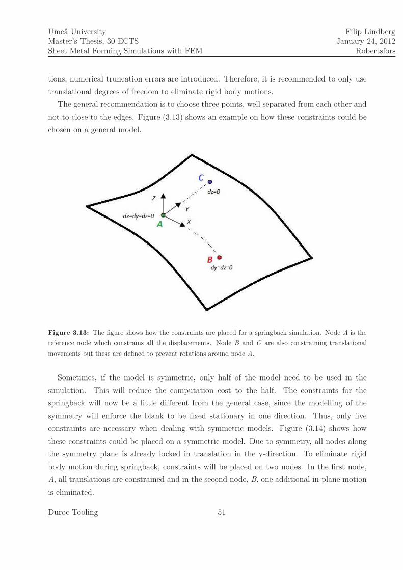
Umeå UniversityMaster’s Thesis, 30 ECTSSheet Metal Forming Simulations with FEM
Filip LindbergJanuary 24, 2012
Robertsfors
tions, numerical truncation errors are introduced. Therefore, it is recommended to only use
translational degrees of freedom to eliminate rigid body motions.
The general recommendation is to choose three points, well separated from each other and
not to close to the edges. Figure (3.13) shows an example on how these constraints could be
chosen on a general model.
Figure 3.13: The figure shows how the constraints are placed for a springback simulation. Node A is the
reference node which constrains all the displacements. Node B and C are also constraining translational
movements but these are defined to prevent rotations around node A.
Sometimes, if the model is symmetric, only half of the model need to be used in the
simulation. This will reduce the computation cost to the half. The constraints for the
springback will now be a little different from the general case, since the modelling of the
symmetry will enforce the blank to be fixed stationary in one direction. Thus, only five
constraints are necessary when dealing with symmetric models. Figure (3.14) shows how
these constraints could be placed on a symmetric model. Due to symmetry, all nodes along
the symmetry plane is already locked in translation in the y-direction. To eliminate rigid
body motion during springback, constraints will be placed on two nodes. In the first node,
A, all translations are constrained and in the second node, B, one additional in-plane motion
is eliminated.
Duroc Tooling 51

Umeå UniversityMaster’s Thesis, 30 ECTSSheet Metal Forming Simulations with FEM
Filip LindbergJanuary 24, 2012
Robertsfors
A way to check that the constraints have been assigned properly is by looking at the forces
at the nodes. The user can set LS-DYNA to calculate the forces at the constrained nodes.
These forces are called SPC-forces. These should be small, typically in the range 0 − 100 N,
otherwise they have probably not been set properly.
Figure 3.14: The figure shows how the constraints are placed in a springback simulation for a symmetric
case. The constraints are placed on two nodes on the symmetry plane. In node A, all displacements are
constrained, eliminating all translational degrees of freedom. In node B, two additional translational degrees
of freedom are constrained to eliminate rigid body rotations about node A.
Run the springback simulation
The simulation of the springback is very fast, usually only a couple of minutes, when compar-
ing to the forming simulations, since only one time step has to used. The explicit method is
very CPU-intensive and the memory usage is relatively low. However, for an implicit solver,
much more memory is used. This has to do with how the solver calculates the next time step.
In an implicit method, a system of equation is solved. Thus, for large models a large matrix
must be inverted, requiring much more memory to store the matrices. However, the models
for forming simulations are very small when comparing to models used in, for example, car
crashing simulations. In car crashing simulations, the memory could be a problem but this
is not likely to occur in forming simulations. Note also, as been mentioned earlier, that dou-
Duroc Tooling 52

Umeå UniversityMaster’s Thesis, 30 ECTSSheet Metal Forming Simulations with FEM
Filip LindbergJanuary 24, 2012
Robertsfors
ble precision should be used in springback simulations, otherwise problems with convergence
might occur. To run a simulation, with one processor, 100 MB RAM and double precision,
the following comand line is written in a DOS-prompt:
C:\LSDYNA\program\ls971_d_R5.1.1_winx64_p.exe I=file_OP15.dyn ncpu=1 memory=100M
3.3.3 Postprocessing
The final stage in the simulation procedure is to evaluate and analyze the results. This can
be done in LS-PrePost, which comes free with LS-DYNA. Generally in sheet metal forming
simulations, we are interested in evaluating the forming process by detecting cracks and
wrinkles that would lead to failure. Another paramter of interest is to find the reaction
forces between the blank and the tools.
Evaluate simulation results
When the simulations are done, it is time to evaluate the results. In a forming process where
there is a trimming step and several forming steps the results are usually evaluated after
every step in the process. If one for example detects problems in the first forming step, one
usually tries to fix these problems before moving on to the next step since if there already
are, for example, cracks in the blank the following simulations may not be realistic. However,
sometimes, even though some problem, such as a crack, is detected in a forming step one
still might want to move on to the next forming step just to get a rough idea of what will
happen in future steps.
The simulations can be evaluated in LS-PrePost. LS-DYNA generates d3plot-files during
the simulations which can be analyzed in LS-PrePost. Each d3plot-file contains one frame
and the user can set how often LS-DYNA should output these files. Usually 10 to 20 output
states are enough for a forming simulation. LS-DYNA will automatically set the number of
output states, but the this can also be set manually. Usually, we are only interested to see
where and approximately when a problem, such as a crack, occured in the simulation and
usually only a few output states are necessary. A problem with using too many output states
Duroc Tooling 53
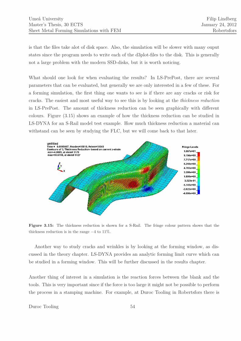
Umeå UniversityMaster’s Thesis, 30 ECTSSheet Metal Forming Simulations with FEM
Filip LindbergJanuary 24, 2012
Robertsfors
is that the files take alot of disk space. Also, the simulation will be slower with many ouput
states since the program needs to write each of the d3plot-files to the disk. This is generally
not a large problem with the modern SSD-disks, but it is worth noticing.
What should one look for when evaluating the results? In LS-PrePost, there are several
parameters that can be evaluated, but generally we are only interested in a few of these. For
a forming simulation, the first thing one wants to see is if there are any cracks or risk for
cracks. The easiest and most useful way to see this is by looking at the thickness reduction
in LS-PrePost. The amount of thickness reduction can be seen graphically with different
colours. Figure (3.15) shows an example of how the thickness reduction can be studied in
LS-DYNA for an S-Rail model test example. How much thickness reduction a material can
withstand can be seen by studying the FLC, but we will come back to that later.
Figure 3.15: The thickness reduction is shown for a S-Rail. The fringe colour pattern shows that the
thickness reduction is in the range −4 to 11%.
Another way to study cracks and wrinkles is by looking at the forming window, as dis-
cussed in the theory chapter. LS-DYNA provides an analytic forming limit curve which can
be studied in a forming window. This will be further discussed in the results chapter.
Another thing of interest in a simulation is the reaction forces between the blank and the
tools. This is very important since if the force is too large it might not be possible to perform
the process in a stamping machine. For example, at Duroc Tooling in Robertsfors there is
Duroc Tooling 54

Umeå UniversityMaster’s Thesis, 30 ECTSSheet Metal Forming Simulations with FEM
Filip LindbergJanuary 24, 2012
Robertsfors
a 1000 tonne press and therefore it is very important that the forces required are less than
this. It is also important to know approximately how large these forces are when setting up
the forming process. For example, study the forming process in figure (3.16). At the initial
stage, both binder 1 and binder 2 are lifted up above the die. Binder 2 is hold up by a force
F . The source of this force may be different depending on what kind of stamping machine is
used. In a hydraulic press, this force comes from the press table, which is controlled by the
hydraulic system. In other stamping machines, gas springs are used to hold up the binder at
the requested force. This force should be high enough to withstand the first forming of the
blank, as shown in (b). When the punch have reached the binder, a larger force is applied
which exceeds the force holding up binder 2. The blank will then move down and be further
formed against the die, as shown in (c).
(a) (b)
(c)
Figure 3.16: (a): The figure shows a forming process where both of the binders, initially, are lifted up
above the die. A force, F, keeps binder 2 stationary. (b): The punch moves down and the blank is formed,
but the binders remain stationary. (c): A larger force which exceeds F is applied, both the binders and the
blank starts to move down and the blank is formed against the die.
The reaction forces also provide a tool for analyzing the forming process. If for example
Duroc Tooling 55

Umeå UniversityMaster’s Thesis, 30 ECTSSheet Metal Forming Simulations with FEM
Filip LindbergJanuary 24, 2012
Robertsfors
an extreme spike, for some of the reaction forces between the tools and the blank, occurs,
or if the forces seem to be unrealistically large, there might be some problem. Sometimes
the prescribed tool motions are maybe by mistake set to move a little too far, or the tools
are desgined such that there will be a through-thickness compression. In that case, the reac-
tion forces will be very large. However, in sheet metal forming processes, through-thickness
compression is not of interest since it generally requires very large forces out of the stamping
machine’s range, thus, the reaction force may tell us that something is wrong and a design
modification should be made, or that the process not is set up properly.
Eventually, when one has found a process that seems to be stable and does not yield cracks
or severe wrinkling it is important to look at the material distribution to see that the formed
detail has the right dimensions as requested. This can be done by importing the CAD-model
for the requested detail and comparing with the model from the simulated results. Probably,
there will be some places where extra material needs to be added and some place where there
is too much material. One then needs to change the trimming lines to get a good blank shape
and then try simulating again. This process is then repeated until the detail is within the
requested tolerances.
Springback compensation
The final stage when designing the forming tools is to make a springback compensation on
the tools. This can be done in Dynaform which has built in special function for springback
compensation. The springback compensation is a purely geometrical operation. The program
takes as input the mesh of the blank before springback, after springback, the desired shape of
the blank, the blank shape after compensation and the mesh of the tools. The desired shape
of the blank and the blank shape after compensation are generally the same as the blank
before springback. The only time when the blank shape after compensation is different is
when the springback compensation is made in several steps. Many times, however, it suffices
to make the springback compensation in one step.
When the springback compensation is run, the program compares the blanks and attempts
to modify the tools to compensate for the springback. The user can set a scaling factor, which
determines how much the compensation should respond to the springback. Springback is a
very complex phenomena and may not aways be linear, therefore, exactly how large the
scaling factor should be might differ depending on the problem. A way to handle this, is by
Duroc Tooling 56

Umeå UniversityMaster’s Thesis, 30 ECTSSheet Metal Forming Simulations with FEM
Filip LindbergJanuary 24, 2012
Robertsfors
running simulations with different scaling factors and analyzing which scaling factor yielded
the best result. By doing this the compensation can usually be made in one step, however, if
the springback compensation is made in several steps this will not be that important scince
the springback will be less in every step and eventually converge.
Another problem with springback compensation is to know at which stage the compensa-
tion should be made. This is the case if the forming is made in several steps. One then have
to look at the springback simulation and see where, on the part, the springback is largest
and find out at which forming step this region could be compensated most efficiently. This
is not a very exact science and experience plays an important role.
Duroc Tooling 57

Chapter 4
Results
In this chapter, the results from the simulations will be presented. Since this thesis is about
development, the process arriving to the final results are more interesting than the final result
itself. Therefore, the results will be presented by showing how the tool design changed over
time, as results from simulations were obtained.
During the development process, there are four different approaches that have been tried
to form the girder. Each of these approaches will be presented here.
4.1 Forming approaches
There are several possible ways to form the girder, however, one way might perhaps be better,
i.e. easier, more stable and cheaper to build. Let us first, again, consider the design of the
girder, see figure (4.1). There are some main features on this girder. One of them being
the flanges at the very ends of the girder. This might be a problematic area, since there are
some small radii where large strains might come in. The flanges at both sides of the girder
are another feature. This might be easier to form, but problems might arise, especially on
the bend, see (b). Finally, there is a bulge at both ends of the girder. When drawing this
bulge, problems with cracks may also appear. Finding a good design, for the tools, to draw
and bend these features, without failure of the material, is the main objective.
58

Umeå UniversityMaster’s Thesis, 30 ECTSSheet Metal Forming Simulations with FEM
Filip LindbergJanuary 24, 2012
Robertsfors
(a) (b) (c)
Figure 4.1: The figure shows different views of the girder. (a): Top view. (b): Side view. (c): Front view.
4.1.1 First approach
In the first approach, the idea was to first make a pure bending and no drawing of the blank
to form the outline of the girder. In the next step the bulge would be drawn and in the last
step the flanges would be bent up. However, we early realised, after some simulations, that
this not would be an efficient method becaused of unnecessary steps and this approach was,
therefore, early dismissed.
4.1.2 Second approach
In the second approach, the blank is formed in two forming steps. In the first forming step,
the blank is bent, as in the first approach, however, the bulge at the very end of the girder
is also drawn in the first step. In the second step, the flanges on the sides are bent up.
We will begin by studying the first version of the tools for the first forming step. Figure
(4.2) shows the process for the first forming stage, first the blank is bent and then the
Duroc Tooling 59

Umeå UniversityMaster’s Thesis, 30 ECTSSheet Metal Forming Simulations with FEM
Filip LindbergJanuary 24, 2012
Robertsfors
bulge is formed. The simulation was run with prescribed tool motions, since the forces were
unknown.
(a) (b)
(c) (d)
Figure 4.2: (a): The figure shows the first forming process where both of the binders, initially, are lifted
up above the die. Binder 2, held up by the hydraulic table, is stationary while binder 1 moves down to hold
the blank. (b): The punch moves down and the blank is formed, but the binders remain stationary. (c): A
force, larger than the force from the hydraulic table, is applied from the punch. Both the binders and the
blank starts to move down and the blank is formed against the die. (d): Perspective view of the tool setup.
The simulation is then evaluated in LS-PrePost. To evaluate the simulation, look at figure
(4.3) showing the thickness reduction in (a) and the FLD in (b). Note the high thickness
reduction, at the top end of the bulge, indicating cracks. The fringe range have been locked
at 30% for better visualization. In fact, the thickness reduction here is above 50%, but that is
not really interesting. The only thing of interest, is if the thickness reduction is large enough
to generate cracks. Steels usually can take somewhere between 30 − 50% thickness reduction
before cracks occur, but this also depends on the thickness of the steel. By looking at the
FLD of the material, one can get an idea about approximately how large thickness reduction
Duroc Tooling 60

Umeå UniversityMaster’s Thesis, 30 ECTSSheet Metal Forming Simulations with FEM
Filip LindbergJanuary 24, 2012
Robertsfors
the material can withstand beforce cracking, see figure (4.4 a). Note that this FLC is for a
sheet with 3 mm thickness, however, we have 6 mm, but this will generally not differ that
much and generally a larger sheet can withstand larger deformations and, thus, we are on
the safe side. Remember, since we assume constant volume, the following relation holds
ǫthick. + ǫ1 + ǫ2 = 0 (4.1)
or
ǫthick. = −ǫ1 − ǫ2 (4.2)
(a) (b)
Figure 4.3: (a): Thickness reduction in the first forming step. The fringe range have been locked at 30%
for better visualization. Note, the high thickness reduction at the top of the bulge, indicating high risk for
cracks. (b): The forming limit dagram (FLD), also indicating cracks at the top of the bulge.
Now, looking at a point, for example, ǫmax = 0.37 and ǫmin = 0 the thickness reduction
will then be ǫthick. = −0.37, i.e. 37%. But one must remember that the FLD is based on
the true strains. Thus a thickness reduction, based on the true strains, corresponds to a
thickness reduction of 1−e−0.37 = 30.9%, see equation (2.67). However, taking a point to the
far right of the FLC, for example, ǫmax = 0.47 and ǫmin = 0.35, we get ǫthick. = −0.82, i.e. a
thickness reduction of 1−e−0.82 = 56.0% . The problem is only that this strain combination is
extremely hard to achieve, therefore 30.9% should serve as a guideline for how much thickness
reduction this metal can take. Figure (4.4b) shows how the elements from a typical forming
simulation are distributed and as can be seen strain combinations to the far right are very
rare.
Duroc Tooling 61

Umeå UniversityMaster’s Thesis, 30 ECTSSheet Metal Forming Simulations with FEM
Filip LindbergJanuary 24, 2012
Robertsfors
(a) (b)
Figure 4.4: (a): The FLC for Domex 500 MC for a sheet with 3 mm thickness. (b): A plot of the strain
distribution in a forming simulation.
One way to see if the thickness reduction yielded a crack is by studying how the thickness
reduction changes during the simulation. If for example, the thickness reduction is 35%
at time, tn. At the next time step, tn+1, where the tools have moved a little further the
thickness reduction make a large jump up to, say 50%. This would clearly indicate that the
blank has failed and a crack is present. This, however, is not always the case. Sometimes,
the thickness reduction is close to the limit wherer a crack would appear and it is hard to
say if the blank would fail. One can then only say that there are risk for cracks and caution
should be taken. Also, looking at the forming limit diagram (FLD) in (4.3b), one sees that
there are indications of cracks at the top of the bulge.
But it is not only high thickness reduction that can be a problem. Negative thickness
reduction can also be unwanted since this may give wrinkles. At the corners of the bulge,
there is a negative thickness reduction which may give wrinkle tendency. Looking at the FLD,
wrinkling tendency and wrinkles are visulalized graphically with blue and purple respectively.
However, as mentioned before, the FLD should be used with caution. There are large regions
of the blank where the FLD indicates wrinkling, which in reality, probably, not is the case.
Sometimes, the FLD could also miss wrinkling even though there are wrinkles present, see
figure (4.5). One can clearly see that there are wrinkles at the very end of the bulge, when
viewed in normal mode, i.e. without any analysis tools. However, when using the FLD to
Duroc Tooling 62

Umeå UniversityMaster’s Thesis, 30 ECTSSheet Metal Forming Simulations with FEM
Filip LindbergJanuary 24, 2012
Robertsfors
study wrinkling, over the same region, it says that the stretching is good. On a small portion
of the region, where wrinkles can be seen in (a), the FLD, at least, indicates some wrinkling
tendency. From this observation, it is obvious that the FLD should be trusted with caution
when it comes to wrinkling. However, as was mentioned in the theory section, the wrinkling
limit is not entirely a material property and is therefore hard to estimate exactly.
(a) (b)
Figure 4.5: (a): A zoom in on the blank, viewed in normal mode. Some wrinkles can be seen. (b): However,
when the same region is studied with the FLD, it indicates good stretching and only some wrinkling tendency
over a small region even though there are obvious wrinkling.
Next, the reaction forces will be studied, see figure (4.6). In figure (a) the reaction forces,
in MN, between the blank and the tools are shown for the first forming step. To easier see
the magnitude of the forces at the beginning of the forming step, figure (b) shows a zoom
in on this region. As can be seen in (a), the reaction forces in the beginning of the process,
i.e. up to t = 0.14, are much smaller. Here, the blank is only bent and no drawing is done.
However, from t = 0.14 to the end of the process, the reaction forces are much larger. Here
the bulge is drawn which requires much larger forces than pure bending. Forces of interest,
are especially the blank/punch and the blank/binder 2 forces. Note, the unit of time is left
out since the solution is time scaled and, therefore, a unit does not make sense.
The blank/punch force is important to know, since if this force would be too large, the
press would not be able to form the piece. Duroc Tooling in Robertsfors has a 1000 tonne, i.e.
10 MN press. Thus, the force should not exceed 10 MN. Also, note that due to symmetry
only half of the model is simulated and hence only half of the forces are calculated. Thus,
these forces must be doubled. The blank/punch reaction force reaches a maximum at about
Duroc Tooling 63

Umeå UniversityMaster’s Thesis, 30 ECTSSheet Metal Forming Simulations with FEM
Filip LindbergJanuary 24, 2012
Robertsfors
3.7 MN and, therefore, the real force is 7.4 MN. This is, hence, acceptable.
The other force of interest, is the blank/binder 2 reaction force. When setting up the
process, it is important to approximately know this force. This force is, in this case, applied
from the hydraulic table, to hold up binder 2 when the blank is bent. The force should be
large enough to keep binder 2 stationary while the blank is bent, but not too large either.
If this force would be too large, once again, the force required by the press could go out of
range. Also the hydraulic table also has a limit on the force it can apply. Looking at figure
(b), one can see that this force reaches a maximum of 0.37 MN, i.e. 0.74 MN, for the full
model, during the bending phase. Binder 2 should, therefore, be held up with a force larger
than 0.74 MN.
Duroc Tooling 64

Umeå UniversityMaster’s Thesis, 30 ECTSSheet Metal Forming Simulations with FEM
Filip LindbergJanuary 24, 2012
Robertsfors
(a)
(b)
Figure 4.6: (a): The reaction forces for the first forming step. Initially, when the blank is bent, the reaction
forces are small. However, when the bulge is drawn, much higher forces are required. (b): A zoom in on
the beginning of the forming process to easier see the magnitude of the forces. Note, due to symmetry, only
half of the model is simulated. Thus, only half of the reaction forces are calculated. To calculate the forces
required, the forces must be doubled.
An attempt was made to try decrease the thickness reduction at the top of the bulge, by
increasing the drawing radius and making the bulge higher. However this would require the
bulge to be further formed in the next forming step to attain the required shape. But this
allows the material to be drawn over a larger region and more material will be availiable at
the top when the bulge should be further formed, see figure (4.7). Note how the thickness
Duroc Tooling 65

Umeå UniversityMaster’s Thesis, 30 ECTSSheet Metal Forming Simulations with FEM
Filip LindbergJanuary 24, 2012
Robertsfors
reduction has been greatly reduced from 50% to 31.3% at the worst region. The FLD indicates
risk for cracks over just a few elements at the top of the bulge. Even though this sheet maybe
would not crack, one should be very careful when one is this close to the limit. Also looking
at how the severe deformations are spread one can see that they focuses locally over just a
few elements. This is also an indication that this is a very problematic region and caution
should be taken.
(a)
(b)
(c) (d)
Figure 4.7: (a): Section plane cut showing the original bulge shape. (b): A modification of the shape with
larger radius to allow the material to be drawn over a larger region. (c): Thickness reduction in the first
forming step. Note, the thickness reduction at the top of the bulge now have been reduced, however, there
are still risk for cracks and also the bulge needs to be further formed in the next step. (d): The FLD still
indicating risk for cracks.
Duroc Tooling 66

Umeå UniversityMaster’s Thesis, 30 ECTSSheet Metal Forming Simulations with FEM
Filip LindbergJanuary 24, 2012
Robertsfors
In the next forming step, the bulge is further drawn and the flanges are bent up. The first
version of the tools for the second forming step is shown in figure (4.8).
(a) (b)
(c)
Figure 4.8: (a): The figure shows the second forming step. The binder is first lifted up. (b): The punch
moves down and the bulge is further formed against the binder. (c): Both the binder and the punch moves
down and the flanges are bent up and the blank is further formed against the die.
The thickness reduction and the FLD, for the second forming step, are shown in figure
(4.9). There is still quite high thickness reduction at the top of the bulge and on the top sides
of the bulge. The FLD indicates some severe thinning and risk for cracks over a few elements.
Even though it maybe would be possible to form the bulge this way without cracking, it is
better to try further lower the thickness reduction to be on the certain side.
On the side flanges, where the girder is bent, very high thickness reduction, almost 90%,
can be seen. Large deformations have focused locally and the result is a crack. Also, at the
Duroc Tooling 67

Umeå UniversityMaster’s Thesis, 30 ECTSSheet Metal Forming Simulations with FEM
Filip LindbergJanuary 24, 2012
Robertsfors
flange at the end of the girder, evident crack indications can be seen where the material have
been forced to bend over a very sharp angle. However, a design change will be made on the
girder since the customer realised that this would be a problematic area. Therefore, we did
not put any work to fix this region for now.
(a) (b)
Figure 4.9: (a): Thickness reduction in the second forming step. The fringe range have been locked at 40%
for better visualization. There is still high thickness reduction on the top sides of the bulge. On the side
flange at the bend, large thickness reduction can be seen indicating a large crack. (b): The FLD.
The first aim was to fix the problems in the region of the bulge. Binder 1, in the first
forming step, was modified to also hold over some part of the bulge to get rid of some of the
wrinkling, see figure (4.10). The bulge shape was also modified, with an even larger drawing
radius, to allow material to be drawn over an even larger region.
As can been seen in the results from the simulation, the bulge starts to look better and
the deformations do not focus locally as before. However, at the top side of the bulge there
are still high thickness reduction, around 40%, which most certainly will give cracks.
Duroc Tooling 68

Umeå UniversityMaster’s Thesis, 30 ECTSSheet Metal Forming Simulations with FEM
Filip LindbergJanuary 24, 2012
Robertsfors
(a) (b)
(c) (d)
Figure 4.10: (a): The figure shows the modified tools for the first forming step. Note also the design change
of binder 1 to reduce the wrinkling tendency at the very end of the bulge. (b): The bulge shape has been
changed again, with an even larger radius to make a smoother drawing and to let material be drawn over
an even larger region. (c): Thickness reduction in the first forming step. Note how the thickness reduction
have been further decreased. (d): Thickness reduction in the second forming step. The fringe range has been
locked at 40%. Cracks will still be a problem at the top sides of the bulge.
We then left the problem at the bulge, for a while, to focus on the the problematic regions
of the flanges, on the sides of the girder, to see if it was possible to somehow avoid cracking.
The tools in the first forming step was changed, such that some parts of the side flanges
were bent up already in the first forming step. The hope was that the material at the critical
region, would not be locked in the same manner, but should be allowed to deform more freely
over the bend such that the deformations would be spread over a larger region and not focus
Duroc Tooling 69

Umeå UniversityMaster’s Thesis, 30 ECTSSheet Metal Forming Simulations with FEM
Filip LindbergJanuary 24, 2012
Robertsfors
locally. Figure (4.11) shows the tools for the first forming step, in (a), and the thickness
reduction, in (b). Compare the tools with the tools in figure (4.8). Note that the side steels
goes all the way in that case, but as can be seen in (a), they end about half the way from the
symmetry line, to only bend up some part of the side flanges. In (b), the thickness reduction
can be seen. The result was better, the right flange looks much better now, however, at the
critial region on the left flange, an evident crack is still there.
(a) (b)
Figure 4.11: (a): The tools for the first forming step. Some parts of the flange are bent up, already, in the
first forming step. (b): The thickness reduction from the simulation. There is still problem on the left flange
where a crack will occur, however, the crack on the right flange is now gone.
Blank shape modifications
To further try sovle the problem with the crack at the side flanges, an attempt was made by
adding and removing material along the edge of the blank. This will make the blank edge
longer and the blank will also be stronger at some places and weaker at other places. If these
modifications are placed in the right manner, it is possible to spread out the stresses over a
larger region and perhaps avoid cracks. Figure (4.12) shows three different versions of the
blank that was used. The red circles indicate where these modifications were placed. In (a),
small radiuses in the cut outs were tested. In (b) and (c) the radiuses of the cut outs have
been increased.
Duroc Tooling 70

Umeå UniversityMaster’s Thesis, 30 ECTSSheet Metal Forming Simulations with FEM
Filip LindbergJanuary 24, 2012
Robertsfors
(a) (b) (c)
Figure 4.12: The figure shows three different versions of the blank that was tested to try spread out the
stresses over a larger region.
The results from the simulations, using the three different blanks, can be seen in figure
(4.13). In (a), with small radiuses on the cut outs, the result is even worse than before.
In (b), however, an improvement can be seen. The radius of the cut out is bigger and the
stresses are allowed to spread over a larger distance, which result in a much smaller crack. In
(c), the radius has been further increased and the result starts to look much better. Notice
the right flange, where the crack has vanished. There are still cracks on the left flange, but
they are smaller.
It would perhaps be possible to get rid of the cracks by further increasing the radiuses and
trying to spread out the stresses even more. However, one must remember that there are
certain tolerances that must be fulfilled on the shape of the girder. The edge is not allowed to
deviate more than a few millimeters from the blueprints. This method, by slightly modifying
the blank shape, would be most useful if one was very close to the desired result. Maybe
only small cracks are present, in that case, it would probably be a good idea to try eliminate
these by slightly modifying the blank shape.
Even though it would perhaps be possible to solve this problem by further trying to modify
the blank shape, we decided to go on to find a more robust method. The flange is not even
bent up completely yet at this step and more problems could arise around the flanges in the
next forming step.
Duroc Tooling 71

Umeå UniversityMaster’s Thesis, 30 ECTSSheet Metal Forming Simulations with FEM
Filip LindbergJanuary 24, 2012
Robertsfors
(a) (b)
(c)
Figure 4.13: The figure shows the thickness reduction for the three different blanks. (a): No improvement
can be seen. The deformation still focuses very locally. (b): The stresses start to spread out over a larger
region and a clear improvement can be seen. (c): The stresses are further spread out and the crack at the
right flange has now been eliminated. On the left flange, cracks are still present, but they are much smaller
now.
4.1.3 Third Approach
The main idea with this approach was not try solve the problems with the cracks at the
bulge. The third approach is a three step forming method. In the first step the bulge is
Duroc Tooling 72

Umeå UniversityMaster’s Thesis, 30 ECTSSheet Metal Forming Simulations with FEM
Filip LindbergJanuary 24, 2012
Robertsfors
preformed. In the second step, the blank is bent and the bulge is further formed. Finally, in
the third step, the flanges are bent up.
The tools for the first forming step is very simple, see figure (4.14 a,b). The binder and
the punch are, initially, above the die. The punch moves down against the binder to hold
the blank. The punch and the binder then moves down to form the blank against the die.
Figure (4.14 c) shows the tools for the second step, it reminds of the first forming step in the
second approach. First binder 1 moves down to hold the blank against binder 2. The punch
then moves down to bend the blank. Finally the tools move down to form the blank against
the die.
(a) (b)
(c)
Figure 4.14: The figure shows the tools for the first forming step. (a): The tools are placed in their initial
positions. (b): The end position for the tools. (c): The initial positions for the second forming step.
Several attempts were made to try form the bulge and the results, from one of the attempts,
can ben seen in figure (4.15). The first forming step, (a), where the bulge is preformed, only
gives a small thickness reduction. In the second forming step the thickness reduction is much
larger, about 40% at the top of the bulge, where cracks will appear. As can be seen, the
result was even worse than before.
Duroc Tooling 73

Umeå UniversityMaster’s Thesis, 30 ECTSSheet Metal Forming Simulations with FEM
Filip LindbergJanuary 24, 2012
Robertsfors
(a) (b)
Figure 4.15: (a): The thickness reduction for the first forming step with a maximum at about 12%. (b):
Thickness reduction in the second forming step. There are still high thickness reduction at the top of the
bulge with risk for cracks.
Once again, we left the bulge for now, to again try find a solution with the side flanges.
The tools for the third forming step are basically the same as the tools in the final forming
step from the second approach. Many attempts were made for the third forming step, but
without any great success. The material still got extremely stiff at the side flanges around
the bend and cracks appear.
One attempt, that led to a small improvement, was by increasing the radius at the side
steel to allow the side flanges to bend up more smoothely. The die and the thickness reduction
can be seen in figure (4.16). As can be seen in (b), even though a small improvement was
done, cracks still appear at both flanges. Perhaps the radiuses on the side steels could have
been further increased, but that only seemed to help slightly. Something more drastically
had to be done.
Duroc Tooling 74

Umeå UniversityMaster’s Thesis, 30 ECTSSheet Metal Forming Simulations with FEM
Filip LindbergJanuary 24, 2012
Robertsfors
(a) (b)
Figure 4.16: (a): The die in the third forming step. Note how the radiuses at the side steels have been
increased to allow smoother bending of the side flanges. (b): Thickness reduction in the third forming step.
Some improvements were made on the right side flange, but cracks still appear.
4.1.4 Fourth Approach
To solve the problem with the cracks at the side flanges, something new had to be done.
An attempt was made by introducing a preforming step where bumps were drawn along the
edge of the blank around the critial region where the blank is bent. These bumps would
then be flattened out in the second forming step such that extra material would be gathered
along the edge. Not only is there extra material, but the edge would also be longer after the
preforming step. Thus, the material would be able to deform even more.
The idea was then to use the same tools from a previous approaches to form the girder.
The tools for the first forming step in the second approach and the tools from the third
forming step in the third approach was used. Since the bulge was even worse in the third
approach, the tools from the second approach was taken instead to form the bulge.
The tools and the thickness reduction from the first step, i.e. the preforming, can be seen
in figure (4.17). The bulges have been placed at the critical regions where cracks have been a
problem. The bulges makes the edge longer and will allow the material to deform even more
at those regions.
Duroc Tooling 75

Umeå UniversityMaster’s Thesis, 30 ECTSSheet Metal Forming Simulations with FEM
Filip LindbergJanuary 24, 2012
Robertsfors
(a) (b)
(c)
Figure 4.17: (a): The tools in the preforming step seen from the side. (b): Tools from a top view. (c):
The thickness reduction. Note also how the bulges have been placed to extend the edge and generate extra
material along the edge of the critial regions.
This blank was then run in the second and a third forming step. The tools for the second
forming step are the same as one of the versions in the second approach, see figure (4.11 a).
The tools for the third forming step is also the same, but the radiuses at the side steels of the
die have been increased, as mentioned in approach three. The results from the simulations
can be seen in figure (4.18).
Duroc Tooling 76

Umeå UniversityMaster’s Thesis, 30 ECTSSheet Metal Forming Simulations with FEM
Filip LindbergJanuary 24, 2012
Robertsfors
(a) (b)
Figure 4.18: (a): Thickness reduction after the third forming step. Notice how the problematic region now
is free from cracks. (b): The FLD for the forming process.
The reaction forces for the third forming step are shown in figure (4.19). At time t = 0.11,
the bulge has been formed and the punch and binder starts to move down into the die. Once
again, remember that the reaction forces must be doubled since only half of the model is
simulated. The binder has a maximal force at 2 · 3 MN = 6 MN, i.e. 600 tonne and that is
out of the limit of what the hydraulic table can achieve. The problem is that some forming,
the bulge, is done against the binder. The required force would be less, by avoiding forming
against the binder and instead trying to do all forming against the die.
Duroc Tooling 77

Umeå UniversityMaster’s Thesis, 30 ECTSSheet Metal Forming Simulations with FEM
Filip LindbergJanuary 24, 2012
Robertsfors
Figure 4.19: The reaction forces for the second forming step. At time t = 0.11, the punch has reached the
binder.
The surfaces, for the forming of the bulge, was moved down to the die instead. Also, to
try further reduce the thickness reduction at the top corners of the bulge, the corners were
lowered slightly and made smoother. The tools and the results from the simulation can be
seen in figure (4.20). Note, in (b), that the thickness reduction at the top of the bulge now
have been decreased and cracks will probably be avoided now. A crack can still be seen at
the right flange, close to the symmetry line. This could be solved by perhaps drawing one
more bump in this region, in the preforming step. There are also two cracks at the very end
of the girder, where the flanges are bent 90. The radiuses is very small and large stresses
appear in this region. However, according to the truck manufacturer, a small design change
will be made here since this is a very problematic region. Therefore, we did not consider the
problems at this region.
In (c), the reaction forces can be seen. The force required by the binder has now been
greatly reduced. The second step was to run the simulation with predefined forces for the
binder rather than with predefined tool motions. Since no forming is done and the binder
is below the blank, the required force by the blank could probably be even smaller than
indicated in the figure. However, if the force is choosen differently the distribution of the
material will be different.
Duroc Tooling 78

Umeå UniversityMaster’s Thesis, 30 ECTSSheet Metal Forming Simulations with FEM
Filip LindbergJanuary 24, 2012
Robertsfors
(a) (b)
(c)
Figure 4.20: (a): The modified tools for the third forming step. The forming surfaces of the bulge have
been moved down to the die to avoid too large forces between the binder and the blank. The corners at the
top of the bulge has also been smoothened out slightly to reduce the thickness reduction. (b): The thickness
reduction after the third forming step. The bulge looks good now and cracks will probably not occur. The
right flange still has a small crack close to the symmetry line. (c): The reaction forces. Note, the reaction
force between the blank and the binder has been greatly reduced.
4.2 Springback compensation
The final step was to make a springback compensation on the tools. First a springback
simulation was made, see figure (4.21) which shows the displacement in the z-direction. As
Duroc Tooling 79

Umeå UniversityMaster’s Thesis, 30 ECTSSheet Metal Forming Simulations with FEM
Filip LindbergJanuary 24, 2012
Robertsfors
can be seen, the girder almost twists when the stresses are relieved in the material. At the
end on the right side the displacement is about 7 mm and on the other side −4 mm . At the
first glance, this might seem to be wrong. But if one looks at girder from the front, figure
(4.1 c), one sees that the girder not is symmetric and one can therefore not assume that the
girder would have symmetric springback.
Figure 4.21: The displacement in the z-direction can be seen showing the springback. Note how the girder
is almost twisted.
The springback is too large to ignore springback compensation in this case. But where
should the springback compensation be made? From the springback simulation, one can see
that the region where springback compensation is most important is at the region which is
mainly formed in the last forming step, therefore, the springback compensation was made on
those tools. Several attempts with different scaling factors, in the range of 0.6 − 1.0, were
tested to achieve good results.
Duroc Tooling 80

Umeå UniversityMaster’s Thesis, 30 ECTSSheet Metal Forming Simulations with FEM
Filip LindbergJanuary 24, 2012
Robertsfors
4.3 Blank Shape
After one has found a method where the forming is acceptable, i.e. does not yield cracks, too
much wrinkling etc, one also has to look at the material distribution such that the formed
part really has the shape requested and that the geometry is within the given tolerances. To
do this, the model, after the simulations, was imported together with the CAD-model of the
girder. The models were placed on top of each other to see where the formed part differed
from CAD-model. The blank geometry was then slightly modified in Solid Works, at places
where the CAD-model differed from the formed part to try get a better material distribution.
Figure (4.22) shows the formed part, after springback compensation, and the CAD-model for
two different cases. In (a), an early simulation can be seen and in (b) the blank shape has
been modified several times to try get the desired shape.
(a) (b)
Figure 4.22: (a): The formed part (brown) and the CAD-model (blue) after springback compensation. The
formed part differs from the CAD-model. The blank shape must be modified to attain the requested shape.
(b): The blank shape has been modified and the formed part is almost identical to the CAD-model.
4.4 Final results
This section presents the final results for the forming simulations after springback compensa-
tion. To remove the crack on the right flange, in figure (4.18), an additional bump was drawn
in the preforming step. Figure (4.23) shows the results for the final forming simulations for
Duroc Tooling 81

Umeå UniversityMaster’s Thesis, 30 ECTSSheet Metal Forming Simulations with FEM
Filip LindbergJanuary 24, 2012
Robertsfors
all the forming steps. As can be seen in (c) and (d), the forming now looks acceptable and
no cracks can be seen, except for the the small radii on the top of the flanges at the far end
of the girder. But, since a design change will be made here, this was left for now. What one
could try to do is to draw additional bumps, in the preforming steps, here to avoid cracking.
(a) (b)
(c) (d)
Figure 4.23: (a), (b): Thickness reduction in the first (preforming) step, and the second forming step
respectively. (c): Thickness reduction after the third forming step. The only region with cracks is at the
small radii on the top of the flanges at the far end of the girder, but, as mentioned before, this was not
considered since a design change will be made here. (d): FLD after the third forming step.
Duroc Tooling 82

Chapter 5
Discussion
In this chapther the results from the results will be further discussed. This is of great
importance in this kind of work. One question that arises is if the simulations can be trusted
and relied on. We will then also discuss how the simulation tool could be implemented
in Durocs production development and if it would be profitable to invest in a simulation
software. Finally some suggestions on further work will be given.
5.1 Simulation software
In this section we will focus on the simulation software. We will discuss the reliability of
the simulations, an efficieny perspective and profits and costs that comes with implementing
a simulation software in the production process. At the end we will also look at a future
perspective in the field of sheet metal forming.
5.1.1 Reliability and robustness
One important aspect to discuss is if the results from the simulations are reliable. This could
be tested by simulating and then performing the same forming operation in reality. One
could then easily measure, for example, thickness reduction over the material and see if the
simulations give the same results. This has, however, not been tested. Another possible
method is to look at some basic examples where one already know that the material, for
example, would fail and then by simulating that process see if the simulations agree with the
expected outcome. This has, however, not been the focus for this thesis. One could make a
83

Umeå UniversityMaster’s Thesis, 30 ECTSSheet Metal Forming Simulations with FEM
Filip LindbergJanuary 24, 2012
Robertsfors
whole thesis just to investige the preciseness of the simulation software. Some simple things
have been tested though. For example, in the preforming step, in the fourth approach, when
the bumps where placed, some different versions where tested. If one places the bumps closer
to each other, one would expect the thickness reduction between the bumps to be higher
than if they were further separated since more material has to be shared between the bumps.
Looking at figure (5.1) one can see the thickness reduction for two different cases where the
bumps have been placed differently. As expected, the thickness reduction is much higher
when the bumps are placed close to each other. This is perhaps not the best example, but
the idea is to show that the simulation software, at least, give the right indication when one
makes a design change. This is the main idea with a simulation tool, not only just to get
some exact quantitatively results, but also just to get an indication of what happens when
one makes a design change.
(a) (b)
Figure 5.1: (a): Thickness reduction in the preforming step. (b): The bumps have been placed closer to
each other and, as expected, the thickness reduction is higher.
Another important thing when discussing reliability is the robustness. Are the simulations
reliable if some parameter is altered slightly, such as the material model? In reality the
material could include variations such as small inhomogeneties. This should, however, not be
a problem if one uses a good material model. The material data that the steel manufacturers
provide are based on minimum values. Thus, the simulations should already be compensated
for such possible variations. In this thesis the anisotropy values, R, have been set to one. In
reality there are usually, however, some difference of the material properties along the different
Duroc Tooling 84

Umeå UniversityMaster’s Thesis, 30 ECTSSheet Metal Forming Simulations with FEM
Filip LindbergJanuary 24, 2012
Robertsfors
directions. This should generally not be a problem. There are two ways to analyze this if
one wants to be more confident. Either one tries to alter the R-values and then simulating
and noticing the difference. Otherwise one must try to get an even better material model,
including these R-values, from the steel suppliers or buy a material test from a university or
some other company that can perform such a test.
A robustness test is more interesting in a springback perspective. The material data is
based on minimum values, increasing the n-value only makes the material more formable and
reduces the risk for cracks. However, the magnitude of the springback could differ. Thus,
one could try to alter the n-value and see if any big difference can be noticed.
No thourough robustness test has been performed in this thesis. The springback was,
however, tested with slightly different n-values, but no big difference could be seen.
One should also remember that many studies about LS-DYNA validity has already been
made. The springback simulations, which are much harder to predict than the normal
forming simulations, have an accuracy at around 75 − 85%, but can reach up to 95%.
[LSTC Inc(2009e)] This also gives some credibility to the simulations results.
5.1.2 Efficiency
Another important question to discuss is the efficieny of the simulation tool. Setting up a
simulation for a forming operation is fairly easy. The big advantage with a simulation tool is
the possibility to test a method and get results relatively quick. What does realtively quick
mean then? For example, the simulation of the last forming step in the fourth approach
takes about five hours running time on an Intel Core i7 CPU 3.20 GHz with 8 GB RAM
using only one CPU. This model has a minimum element size of 4 mm and about 31 000
elements totally. This is a relatively large model which could probably be minimized with
fewer elements without loosing accuracy of the results. How long time the simulation will
take depends on how long the tool motions are and also the size of the model. Usually the
forming parts are much smaller than this and therefore the model would also be smaller.
Thus, this can be seen, as the maximum time a normal forming simulation would take for
Duroc Tooling.
Now, this should be compared to the time it would take to test a method or a design
change without using a simulation software. In that case one would have to actually build
Duroc Tooling 85

Umeå UniversityMaster’s Thesis, 30 ECTSSheet Metal Forming Simulations with FEM
Filip LindbergJanuary 24, 2012
Robertsfors
the tools and perform the forming process in a stamping machine. The time to just make a
small design change, such as changing the radius on some tool, is many factors larger than
the time it takes to get results from a simulation. Another problem with making design
changes in reality is if one would have to add material to a tool. This could be the case if the
radius would have to be changed or if the side steels would have to be made higher. Generally
when a radius should be increased, material will be removed and if a radius should be made
smaller material will have to be added. The only problem with adding material is that it is
almost impossible to do without rebuilding the tools. It is easier to take away material and
increase a radius by trimming. Luckily, the radiuses usually have to be made larger if the
material has failed, but this might not always be the case. Also, to actaully build the tools
in reality requires many people and also costly machine hours. The difference in cost could
probably differ with about 1000 − 3000 kr for a simulation up to maybe 20 000 − 80 000 kr
when building the tools in reality. This is, however, not really a fair evaluation either since
one would also have to build the tools after simulating. But if the results did not come out
right, which many times is the case, this would be true. The difference in time would perhaps
be 5 hours for a simulation and 40 − 200 hours when building the tools in reality. This could
be even worse if the forming is made in several stages. If one makes a design change in one
step, the tools in the other steps could also need to be modified making the work even more
troublesome.
The blank shape is also another thing that has to be tested. From the simulations it has
been seen that finding a good blank shape requires several trial and errors before meeting the
required tolerances. This is, however, a smaller concern since the blank shape can be altered
much easier than the forming tools. But, as was found from the results, modifing the blank
shape does not only alter the geometry but could also change how the stresses are distributed
within the material which could lead to cracks that previously not were a problem.
Finally, the springback compensation is the last problem. Springback is a difficult phe-
nomena due to non-linearity and also that a small angular springback could result in large
deformations of the whole part. As was seen in the results, guessing how the springback
would look like is extremely hard and non-intuitive. Thus, trying to springback compen-
sate without using simulations could be extremely dangerous since one might do that totally
wrong. Even though springback simulations not may be exact either, due to its complexity,
a simulation tool may at least give an indication on what the springback will look like and
one will not be totally surprised by the result. Hence, it is better to springback compensate
Duroc Tooling 86
Umeå UniversityMaster’s Thesis, 30 ECTSSheet Metal Forming Simulations with FEM
Filip LindbergJanuary 24, 2012
Robertsfors
than not to do it at all.
From this discussion it is obvious that the efficieny in using a simulation software is
superior and almost a must if one deals with complicated geometries where several trial and
errors might come in. Going into a difficult project without using simulations would be really
dangerous and making a small error could erase the whole profit from the project. Also, using
a simulation software allows one to try ideas that one has none experience of. For example,
if one had not used simulations for this girder, one probably would not have dared to test
the preforming step. New tools must be built which could be extremely costly if it later was
shown that it was of no use. Simulations allows one to test ideas that, for some, might seem
to be taken out of the blue. Thus, without a simulation software the company is compelled
to work within very narrow boundaries and only to use methods that previously have been
tested. A simulation software would, therefore, serve to open up to new thinking and perhaps
advance the company and taking it one step ahead.
5.1.3 Profits and costs
The profits of using a simulation software has already been discussed to some extent, but we
will continue the discussion here. From the efficiency discussion it is clear that one of the
profits could come in terms of a faster and smoother development process of the forming tools.
But there is also a cost related to simulations. First, the software is quite expensive. One
license for LS-DYNA, i.e. for one processor only, costs about 40 000 kr annually. However, if
one buys more licenses the cost is decreasing exponentially. How many licenses that is needed
depends on what simulation times one can accept. More licenses means shorter simulation
times. For Duroc Tooling it would probably, at least initially, suffice with one license. The
preprocessor DynaForm costs a little bit more, around 60 000 kr annually. However, one could
also use the free preprocessor LS-PrePost that comes with LS-DYNA. One should remember,
though, that the free version is more complicated and one can expect longer times to set
up a simulation. The big cost, however, is not the software but the staff that should do
the simulations. One could probably calculate with a cost at about 400 000 − 600 000 kr
annually. However, it is not maybe necessary to work full time with simulations, perhaps it
would be possible to work 50% with simulations and 50% with design engineering in CAD.
The cost for simulations would then decrease. But this depends on how the company wishes
to profilate. If the company would focus mainly on forming tools a bigger need for forming
Duroc Tooling 87

Umeå UniversityMaster’s Thesis, 30 ECTSSheet Metal Forming Simulations with FEM
Filip LindbergJanuary 24, 2012
Robertsfors
simulations would of course arise. It should also be remembered that some forming tools
are much easier to design where the geometry is simpler, the sheet thickness is lower and
the material more formable. In these cases it is not certain that simulations are necessary
to design the tools, however, generally it will probably most times still increase the efficieny
in the designing process anyway. There is also the option to buy simulations externally, for
example, from DynaMore in Linköping. If Duroc mainly wants to focus on simpler forming
tools, this might be a good option and only buy simulations when working with difficult
forming tools. The problem is only that buying simulations externally is extremely costly
and one do not have the same option to try different ideas during the designing process as
when one has simulation in the house.
Another important aspect to discuss when it comes to profits and costs is how the compe-
tition looks like for forming tool producers. In Sweden there are a few companies that work
with forming tools, Duroc Tooling in Robertsfors, Lidhs, Swepart Verktyg and Volvo. Lidhs
uses LS-DYNA, Swepart uses some simulation software and Volvo as well. [Lidhs(2010)]
However, Volvo mainly produces tools for its own use. The main competitors can, therefore,
be seen as Swepart and Lidhs which both uses simulations. For a customer, the company
gets more reliable and trustworthy when it has access to simulation since the customer can
expect a safer production and also that the orders will be delivered in time, since the risk
for unexpected scenarios will be minimized. Also, as the market gets more and more global
the competition gets higher since the customer gets more companies worldwide to buy tools
from. Thus, a simulation software would probably allow the company to get more orders.
Other profits with simulations come in terms of the possibility to take more orders that
otherwise would be to risky to take. Another advantage is also to avoid going in to projects
that may be too difficult, even with access to a simulation tool. For example the girder in
this thesis, would be extremely hard and almost impossible to form without cracks with the
current design. With help of a simulation software, one can tell the customer that some
design changes need to be made in order to form the girder. Finally, since time and costs
become more predictable to calculate when using a simulation software it is also easier to
give a more accurate price to the customer and avoid setting it too low.
Duroc Tooling 88

Umeå UniversityMaster’s Thesis, 30 ECTSSheet Metal Forming Simulations with FEM
Filip LindbergJanuary 24, 2012
Robertsfors
5.1.4 Future
Another aspect that is important to discuss, when considering making an investment of this
sort, is how the future looks in the field of sheet metal forming. Will the forming tools have
to be more advanced in the future such that the need for a simulation tool will be even more
important? The trend is obviously that the formed parts tend to get more complicated. One
of the reasons for this, is that the vehicle industry wants to reduce the number of parts in
the vehicle. Instead of having three parts put together, one wants to form all this parts into
a single part. This will make the geometries more complicated and thus even more difficult
to form.
The vehicle industry, primarily, also strives to make the parts lighter all the time. To
accomplish this, the sheet metal thickness have to be reduced. But if the thickness is reduced
the strength of the parts will also decrease. Therefore, higher strength materials must be
used to compensate for this. As can be understood from reading the theory section about
materials, formability and strength of the materials goes in different directions. Thus, a
high strength material will have lower formability than a low strength material. Not only is
the formability a problem with high strength materials, but the springback also gets more
problematic since high strength materials have larger springback. Therefore, the need to
springback compensate will also be more important in the future.
Another phenomena that has appeared is blanks with several different materials. Two
different materials are welled together into a single blank which is then formed. This is also
something that will make the forming more difficult and harder to predict.
To summarize this, one can expect the forming operations in the future to be more dif-
ficult and troublesome in terms of more complicated geometries, less formale materials and
problematic springback. Thus, from a future perspective, the need for an invesment in a
simulation software will be even greater to meet the future demands.
5.2 The girder
In this section, the final results from the simulations of the girder will be discussed. Would
it be possible to form the girder with the current design of the forming tools? Should this be
the final design or should there still be some modifications. Except for the small radii on the
top of the flanges at the far end of the girder where cracks appear, the simulations indicate
no cracks. At the top bulge, figure (4.23d), there are, however, severe thinning which not
Duroc Tooling 89

Umeå UniversityMaster’s Thesis, 30 ECTSSheet Metal Forming Simulations with FEM
Filip LindbergJanuary 24, 2012
Robertsfors
should be a big problem, but to really be on the safe side it is perhaps a good idea to try
lower the thickness reduction by further increasing the radius of the bulge, see figure (4.10).
Also the corners could maybe be smoothened out slightly to reduce the thickness reduction.
The blank shape is good and the formed part should be within the reuqired tolerances of
±2 mm at the edges.
Another thing that not have been mentioned is how the thickness reduction affects the
strength of the final product. When the customer designs their part they model it with
homogen material, i.e. 6 mm thickness everywhere, however, this can not be fullfilled in
reality since there will be some parts with less material and some parts with excess mate-
rial. However, the engineers in, for example, the vehicle industry are well aware of this and
designs their product to compensate for such variations in homogenity. The customers also
have a set tolerance for how large thickness reduction that can be tolerated. How large this
tolerance is depends on the product and in some cases the tolerances are very narrow. But
with complicated parts, such as this girder the tolerances are usually set quite generous since
the customer is aware of the problems with forming.
The hope was to be able to form the piece in only two steps. However, a preforming step had
to be introduced to deal with the cracks on the side flanges. The cost for having to produce
an extra tool is costly and also when the blanks should be pressed, several tools need to be
used which makes the forming more time consuming. It would perhaps be possible to avoid
the preforming step by somehow trying to add the bumps in the second forming step. This
will require some thinking but may be possible to do. Due to lack of time we did not have
time to implement this now. We priortized to at least find a stable method that could form
the piece, even though this would mean a higher production cost. If these tools should be
produced in the future it would be a good idea to ,at least, try to do it in a two step forming
process since this could save alot of money.
5.2.1 Optimization and time
Here optimization means optimization of the simulation time. Could the model be reduced
to allow even faster simulation times? There are mainly two things that could be done to
reduce the simulation time. First, the model used has a very fine mesh that definitely could
be made more coarse to reduce simulation time. A very fine mesh has been used to be certain
Duroc Tooling 90

Umeå UniversityMaster’s Thesis, 30 ECTSSheet Metal Forming Simulations with FEM
Filip LindbergJanuary 24, 2012
Robertsfors
that the solution not is mesh-dependent. With more experience one could learn more on how
fine the mesh needs to be. However, at an early stage it could be wise to use a coarse mesh
to be able to fast test different ideas. Then as one find a method that seems good one makes
a finer mesh to check the accuracy of the results.
The speed of tools is also another thing that could be further optimized to speed up the
simulations. As already mentioned, the speed can be as fast that no dynamic effects are
introduced in the simulations. In this project, the speed of the tools have been set low
enough to be sure that this is true. However, it would certainly be possible to increase the
speed of the tools and still get the same results. This is something one could experiment
more with to optimize the simultion time.
Finally the initial placement of the tools can also be slightly optimized. It is a good idea
to place the tools as close to the blank as possible to avoid unnecessary tool motions that
increases the simulation time. But it is important to really check that there, initially, not
are any penetration of the tools into the blank.
5.3 Main conclusions
There are some main concluisions that can be drawn from this project. Was the project
successful? The main objectives were met and even though the hope was to be able to de-
sign the girder in two forming steps only, we finally reached a feasible solution. The main
objectives was to design the tools for forming the girder and then evaluate if investment in
simulation software would be profitable for Duroc Tooling. The answer to the question if
this would be profitable, as can be understood from reading the discussion, depends greatly
on how Duroc Tooling chooses to profilate. If Duroc Tooling focuses on forming tools and
especially advanced forming tools, an investment in simulation software would most certainly
be profitable in terms of more orders, faster and cheaper production and safer production.
However, if Duroc Tooling only produces a few forming tools per year, buying simulations
externally, only when necessary, would maybe be a better option. But from a future per-
spective, one can expect the forming operations to be even more complicated and the need
for a simulation software will rise quickly as the demands on the products get higher.
Another important aspect that was learned during this project is that if one encounters
problems during the forming with, for example, large cracks one usually has to make a drastic
design change. Making small design changes usually have very small effect on the results.
Duroc Tooling 91

Umeå UniversityMaster’s Thesis, 30 ECTSSheet Metal Forming Simulations with FEM
Filip LindbergJanuary 24, 2012
Robertsfors
One can try to alter the friction coefficient or try to explain the forming problems on some
other small parameter, but the difference will be negligible. If there is a severe forming
problem, something drastic has to be made.
Below are some of the main conclusions from this project listed:
• LS-DYNA has shown to be good for setting up forming simulations and also to simulate
springback.
• Designing complicated forming tools without a simulation software compels the de-
sign engineer to work within in very narrow boundaries and only use ideas that have
previously been tested.
• A simulation software is a must if the company wants to be a leading company special-
ized on forming tools.
5.4 Further work
Below are some suggestions listed on further work that can be interesting for Duroc Tooling.
• Make a thorough stability and robustness research of the forming simulations.
• Optimize the simulation time by reducing the elememts in the model and increasing
the tool velocity without changing the results.
• Make a research of a forming process where real data is availabe and compare with
simulation results to analyze the accuracy of the simulations.
• The simulations give alot of data that would be hard to measure on the real material.
Make a study to see how to improve the quantitive analysis by using the simulation
data to guide the lab measurements.
• Make a study on hot-forming simulations using LS-DYNA.
Duroc Tooling 92

Bibliography
[Anders E W Jarfors(2000)] Torgny Carlsson Anders E W Jarfors. Tillverkningsteknologi.
Studentlitteratur, KTH - Materialvetenskap, 2000.
[ASTM(2012)] ASTM. ASTM E2218-02, JAN 2012. URL http://www.astm.org/
Standards/E2218.htm. Last visited 2012/01/11.
[Bradley N. Maker, Xinhai Zhu(2000)] Bradley N. Maker, Xinhai Zhu. Input Parameters
for Metal Forming Simulations using LS-DYNA, APR 2000. URL http://www.
feainformation.com/forming_parameters2.pdf. Last visited 2012/10/03.
[Bradley N. Maker, Xinhai Zhu(2001)] Bradley N. Maker, Xinhai Zhu. Input Parameters for
Springback Simulation using LS-DYNA, JUN 2001. URL http://www.dynalook.com/
Personally/springback_maker_zhu.pdf. Last visited 2012/10/03.
[Dahlberg(2001)] Tore Dahlberg. Teknisk Hållfasthetslära. Studentlitteratur, Linköpings
University - IKP, 2001.
[DynaMore Nordic(2011)] DynaMore Nordic. References, SEP 2011. URL http://www.
dynamore.se/references/. Last visited 2012/01/11.
[eta/DYNAFORM team(2009)] eta/DYNAFORM team. eta/DYNAFORM - Application
Manual. Engineering Technology Associates Inc., 2009.
[FEA-information Inc.(2009)] FEA-information Inc. LS-DYNA Applications, JAN
2009. URL http://www.ls-dyna.com/1_pages/1capabilities.htm. Last visited
2012/01/13.
[Larson and Bengzon(2010)] Mats G. Larson and Fredrik Bengzon. The Finite Element
Method: Theory, Implementation and Practice. Springer, January 2010.
93

Umeå UniversityMaster’s Thesis, 30 ECTSSheet Metal Forming Simulations with FEM
Filip LindbergJanuary 24, 2012
Robertsfors
[Lidhs(2010)] Lidhs. Simulering, JUN 2010. URL http://www.lidhs.se/swe/simulering.
htm. Last visited 2012/01/11.
[Livermore Software Technology Corporation(2006)] Livermore Software Technology Corpo-
ration. LS-DYNA Theory Manual. Livermore Software Technology Corporation, March
2006.
[LSTC(2011)] LSTC. LS-DYNA, AUG 2011. URL http://www.lstc.com/node/16. Last
visited 2012/01/11.
[LSTC Inc(2009a)] LSTC Inc. LS-DYNA Support - Explicit Analysis, SEP 2009a.
URL http://www.dynasupport.com/tutorial/getting-started-with-ls-dyna/
the-next-step. Last visited 2012/01/11.
[LSTC Inc(2009b)] LSTC Inc. LS-DYNA Support - How Contact Works, SEP 2009b.
URL http://www.dynasupport.com/tutorial/contact-modeling-in-ls-dyna/
how-contact-works. Last visited 2012/01/11.
[LSTC Inc(2009c)] LSTC Inc. LS-DYNA Support - Is there a way to reduce the penetrations
problem?, MAY 2009c. URL http://www.dynasupport.com/faq/metal-forming/
is-there-a-way-to-reduce-the-penetration-problem. Last visited 2012/01/11.
[LSTC Inc(2009d)] LSTC Inc. LS-DYNA Support - Double Precision?, SEP 2009d.
URL http://www.dynasupport.com/howtos/general/double-precision. Last vis-
ited 2012/01/11.
[LSTC Inc(2009e)] LSTC Inc. I have no experience in springback prediction, and have no
idea whether my prediction is reasonable. Do you have any idea how accurate the so-
lution could be from LSDYNA? , SEP 2009e. URL http://www.dynasupport.com/
faq/metal-forming/i-have-no-experience-in-springback-prediction-and. Last
visited 2012/01/24.
[Marciniak(2002)] Z. Marciniak. Mechanics of Sheet Metal Forming. Butterworth-
Heinemann 2002, second edition, 2002.
[Metallurgical Consultants(2010)] Metallurgical Consultants. Ductile and Brittle Failures,
SEP 2010. URL http://www.materialsengineer.com/CA-ductbrit.htm. Last visited
2012/01/11.
Duroc Tooling 94
Umeå UniversityMaster’s Thesis, 30 ECTSSheet Metal Forming Simulations with FEM
Filip LindbergJanuary 24, 2012
Robertsfors
[Peir´o and Sherwin(2005)] Joaquim Peir´o and Spencer Sherwin. Handbook of Materials
Modeling, volume II. Springer, 2005. URL http://www2.imperial.ac.uk/ssherw/
spectralhp/papers/HandBook.pdf.
[SSAB(2011)] SSAB. Input Parameters for Springback Simulation using LS-DYNA, SEP
2011. URL http://www.ssab.com/en/Products--Services/Service--support/
Technical-Tools/Steelfacts/Steelfacts/. Last visited 2012/01/13.
Duroc Tooling 95