master thesis, integration of regulatory sequence and gene...

ChristianMommerskamp, BSc.

Master Thesis

Integration of regulatorysequence and gene expression

data.

Institute for Genomics and Bioinformatics,Graz University of Technology

Petersgasse 14, 8010 Graz, AustriaHead: Univ.-Prof. Dipl.-Ing. Dr.techn. Zlatko Trajanoski

Supervisor:Dipl.-Ing. Dr.techn. Hubert Hackl

Evaluator:Dipl.-Ing. Dr.techn. Hubert Hackl

Graz, March 2010

Statutory Declaration

;I declare that I have authored this thesis independently, that I have notused other than the declared sources / resources, and that I have explicitlymarked all material which has been quoted either literally or by contentfrom the used sources.

Graz, ...................... ............................................(date) (signature)

1

Abstract

English

Cell differentiation is often regulated by some key players (transcription fac-tors) activating specific genes being mainly responsible for the formation ofthe respective phenotype. Public available gene expression data on earlymyogenesis and prediction of regulatory sequences (potential transcriptionfactor binding sites) were used to gain insights into the regulatory process ofmuscle cell development. Several methods based on different mathematicalbackground were applied to integrate this two types of data: over represen-tation analysis of transcription factor binding sites of co-expressed genes,binding association with sorted expression (BASE) and network componentanalysis (NCA). A combined strategy for these three methods applied on thesame underlying data led to already known transcription factors like MyoDand the MEF family playing a key role in myogenesis. Some transcriptionfactors were identified previously not associated with the myogenesis process.

Keywords:Myogenesis, gene expression, transcriptional regulation, net-work component analysis, binding association with sorted expression.

2

German

Die Differenzierung von Zellen wird haufig von Transkriptionsfaktoren reg-uliert, die jene fur die phanotypische Entwicklung verantwortlichen Geneaktivieren. Offentlich verfugbare Genexpressionsdaten der fruhen Myoge-nese und Daten uber potentielle Bindungsstellen von Transkriptionsfaktorenwurden verwendet, um einen Einblick in die regulatorischen Prozesse derEntwicklung von Muskelzellen zu erhalten. Es wurden mehrere, auf unter-schiedlichen mathematischen Grundlagen basierende Methoden angewandt,um diese Daten zu integrieren. Die verwendeten Methoden waren die Analysevon uberreprasentierten Transkriptionsfaktor Bindungsstellen co- exprim-ierter Gene, Binding Association with Sorted Expression (BASE) und Net-work Component Analyse (NCA). Durch eine kombinierte Strategie dieserdrei Methoden, die auf die gleichen zugrundeliegenden Daten angewandtwurde, konnten sowohl bekannte Transkriptionsfaktoren der Myogenese (MyoD und Mitglieder der MEF - Familie) als auch bisher nicht mit der Myo-genese assoziierte Transkriptionsfaktoren identifiziert werden.

Stichworter: Myogenese, Genexpression, Regulation durch Transkrip-tionsfaktoren, regulatorische Sequenzen, Network Component Analyse, Bind-ing association with sorted expression.

3

Contents

List Of Figures 6

List Of Tables 8

Glossary 9

1 Introduction 111.1 Myogenesis . . . . . . . . . . . . . . . . . . . . . . . . . . . . 111.2 Gene expression profiling . . . . . . . . . . . . . . . . . . . . . 121.3 Transcriptional regulation and regulatory sequences . . . . . . 131.4 Integration methods . . . . . . . . . . . . . . . . . . . . . . . 141.5 Objectives . . . . . . . . . . . . . . . . . . . . . . . . . . . . . 14

2 Methods 162.1 Underlying data . . . . . . . . . . . . . . . . . . . . . . . . . . 17

2.1.1 Expression matrix . . . . . . . . . . . . . . . . . . . . . 172.1.2 Connectivity matrix . . . . . . . . . . . . . . . . . . . 182.1.3 Data preparation for analysis . . . . . . . . . . . . . . 20

2.2 Clustering . . . . . . . . . . . . . . . . . . . . . . . . . . . . . 202.2.1 Figure of merit (FOM) . . . . . . . . . . . . . . . . . . 202.2.2 k-Means clustering . . . . . . . . . . . . . . . . . . . . 21

2.3 Over representation analysis . . . . . . . . . . . . . . . . . . . 222.3.1 Fisher’s exact test . . . . . . . . . . . . . . . . . . . . 222.3.2 Benjamini and Hochberg correction . . . . . . . . . . . 232.3.3 Z-test . . . . . . . . . . . . . . . . . . . . . . . . . . . 242.3.4 Bonferroni correction . . . . . . . . . . . . . . . . . . . 24

2.4 BASE - Binding Association with Sorted Expression . . . . . . 252.4.1 Mathematical considerations . . . . . . . . . . . . . . . 25

2.5 NCA - Network Component Analysis . . . . . . . . . . . . . . 262.5.1 Mathematical considerations . . . . . . . . . . . . . . . 27

2.6 Applied Tools . . . . . . . . . . . . . . . . . . . . . . . . . . . 28

4

3 Results 303.1 Co-expressed genes during myogenesis . . . . . . . . . . . . . 313.2 Over representation . . . . . . . . . . . . . . . . . . . . . . . . 323.3 BASE . . . . . . . . . . . . . . . . . . . . . . . . . . . . . . . 343.4 NCA . . . . . . . . . . . . . . . . . . . . . . . . . . . . . . . . 363.5 Result comparison . . . . . . . . . . . . . . . . . . . . . . . . 383.6 Gene regulatory network . . . . . . . . . . . . . . . . . . . . . 39

4 Discussion 42

A Clustering and over representation 44

B BASE 49

C NCA 56

5

List of Figures

1.1 Myogenesis reduced to three steps. . . . . . . . . . . . . . . . 121.2 Transcription factor gene activation . . . . . . . . . . . . . . 14

2.1 Analysis strategy . . . . . . . . . . . . . . . . . . . . . . . . . 162.2 The interesting region for possible binding locations . . . . . . 192.3 MyoD Sequence logo . . . . . . . . . . . . . . . . . . . . . . . 192.4 Position Weight Matrix - M00001 MyoD . . . . . . . . . . . . 192.5 NCA- Regulatory Network adopted from [25] . . . . . . . . . . 28

3.1 Expression matrix genes - Temporal behavior. . . . . . . . . . 313.2 Similarity of genes in cluster #1. . . . . . . . . . . . . . . . . 323.3 Gene Ontology (GO) - Cluster # 1 . . . . . . . . . . . . . . . 333.4 Gene regulatory network - condition one . . . . . . . . . . . . 403.5 Gene regulatory network - condition two . . . . . . . . . . . . 403.6 Gene regulatory network - condition six . . . . . . . . . . . . 41

B.1 Temporal behavior - BASE - binary connectivity matrix . . . 49B.2 Temporal behavior - BASE - weighted connectivity matrix . . 51

C.1 Regulatory signals - NCA binary connectivity matrix. . . . . . 56C.2 Regulatory signals - NCA weighted connectivity matrix. . . . 57

6

List of Tables

2.1 Fisher’s exact general contingency table . . . . . . . . . . . . . 222.2 Example: Fisher’s exact contingency table . . . . . . . . . . . 22

3.1 ORA and PScan result cluster 1 . . . . . . . . . . . . . . . . . 333.2 BASE - weighted connectivity matrix - transcription factors . 353.3 BASE - binary connectivity matrix - transcription factors . . . 363.4 NCA - binary connectivity matrix || weighted connectivity ma-

trix - TFs . . . . . . . . . . . . . . . . . . . . . . . . . . . . . 37

A.1 ORA and PScan result cluster 1 . . . . . . . . . . . . . . . . . 44A.2 ORA and PScan result cluster 2 - Part1 . . . . . . . . . . . . 45A.3 ORA and PScan result cluster 2 - Part2 . . . . . . . . . . . . 46A.4 ORA and PScan result cluster 3 . . . . . . . . . . . . . . . . . 46A.5 ORA and PScan result cluster 4 . . . . . . . . . . . . . . . . . 47A.6 ORA and PScan result cluster 5 . . . . . . . . . . . . . . . . . 47A.7 ORA and PScan result cluster 6 . . . . . . . . . . . . . . . . . 48

B.1 BASE - binary connectivity matrix - Group #1 . . . . . . . . 50B.2 BASE - binary connectivity matrix - Group #2 . . . . . . . . 52B.3 BASE - binary connectivity matrix - Group #3 . . . . . . . . 52B.4 BASE - binary connectivity matrix - Group #4 . . . . . . . . 53B.5 BASE - weighted connectivity matrix - Group #1 . . . . . . . 54B.6 BASE - weighted connectivity matrix - Group #2 . . . . . . . 54B.7 BASE - weighted connectivity matrix - Group #3 . . . . . . . 55B.8 BASE - weighted connectivity matrix - Group #4 . . . . . . . 55

C.1 NCA - binary connectivity matrix - Group #1 . . . . . . . . . 58C.2 NCA - binary connectivity matrix - Group #2 . . . . . . . . . 58C.3 NCA - binary connectivity matrix - Group #3 . . . . . . . . . 59C.4 NCA - binary connectivity matrix - Group #4 . . . . . . . . . 59C.5 NCA - weighted connectivity matrix - Group #1 . . . . . . . . 59C.6 NCA - weighted connectivity matrix - Group #2 . . . . . . . . 60

7

C.7 NCA - weighted connectivity matrix - Group #3 . . . . . . . . 60C.8 NCA - weighted connectivity matrix - Group #4 . . . . . . . . 61

8

Glossary

DNA Deoxyribonucleic acid contains genetic instructions for developing andfunctioning of living organisms. In the DNA a lot of information iscoded. Segments of the DNA containing information on proteins andRNA are called genes. The DNA is organized in a double strandedthree dimensional helix.

RNA Ribonucleic acid is very similar to DNA. One of the main differencesis that RNA is usually single-stranded and it is transcribed from DNA.Depending on the context of RNA occurrence it is named a little dif-ferent.

cDNA Complementary DNA (cDNA) is a synthesized DNA which is usedfor microarray production. It is synthesized on the array’s surface as asingle strand sequence.

RefSeq ID Reference Sequence is a comprehensive, integrated, non-redundant,well-annotated sequence which could be an ID for genomic DNA, tran-scripts and proteins. The Reference Sequence collection is adminis-trated by the National Center for Biotechnology Information.

Affymetrix ID Is an identifier used for sequences spotted on an Affymetrixmicroarray to be able to find out which sequence was used during anal-ysis.

Matrix ID Is an identifier which represents the Jaspar or Transfac name ofthe PWM. It is named by the appropriate nomenclature of the respec-tive provider.

PWM - Position Weight Matrix Is a representation of specific motifsused for analysis in biological processes. The used alphabet in motifcontext is A,C,T and G which represents the four bases of coded bio-logical information, e.g. in DNA. Each character is weighted over thepossible sequence length and using them to determine possible bindinglocations the weight is important.

9

TSS - Transcription start site Is the start position within a genome wherethe transcription of a gene is initiated.

10

Chapter 1

Introduction

In biological systems a lot of regulatory interaction takes place during dif-ferent cellular processes. Cell differentiation is often regulated by some keyplayers (transcription factors) activating specific genes being mainly respon-sible for the formation of the respective phenotype. To gain insights in theregulatory mechanisms different experimental and computational methodolo-gies have been developed. High throughput technologies such as mircoarrayanalysis are used to get a significant amount of cell wide data on the molecularlevel and one is able to create meaningful information by analyzing these datathereby. There are also technologies to study regulatory mechanisms such asprotein (transcription factor) DNA binding. By combining both approachesthe possibility understanding these processes in more detail increases andhelps to identify possible new and unknown interactions. Here, based on theexample of muscle cell development (myogenesis), it was studied how celldifferentiation is regulated. For this purpose different integration methodson public available gene expression data and the occurrence of regulatorysequences (motifs) were applied.

1.1 Myogenesis

Myogenesis is the biological process through which the cell differentiationand furthermore the development of muscle cells is initiated [1]. During earlystages of Myogenesis some transcription factors such as MyoD a protein whichbelongs to Myogenetic Regulatory Factors (MRF) and the Myocyte EnhanceFactors (MEF) - family are responsible for muscle cell differentiation [2] [3][4]. Figure 1.1 illustrates this complex biological process. The process ofmyogenesis can be seen as a four step process.

• Starting at pre-myoblast cells so called mesodermal progenitors which

11

are influenced by different transcription factors and proteins lead tomyoblasts.

• Myoblasts themselves are as well a type of progenitor cells of earlymyotubes.

• These early myotubes finally lead to muscle fibers in the next develop-ment step.

• Finally a special quantity of theses muscle fibers together build up amuscle.

Figure 1.1: Myogenesis reduced to three steps.

1.2 Gene expression profiling

Gene expression profiling is a method which is used in molecular biologyto identify the activity, in more detail the expression of a huge amount ofgenes in one analyzing step. There are a number of different high throughputmethods available for this task, e.g. microarray technology. Oligonucleotidesare in situ synthesized or spotted on a modified glass slide. The synthesizingprocess is based on photo lithography explained in more detail in [5]. Thereare different companies, e.g. Affymetrix, which provide standardized arraysfor microarray analysis commonly used for many applications. Preparationof samples to be analyzed is the next step in this context. Commonly totalRNA is used, reverse transcribed to cDNA, labeled with fluorescent dyes,and hybridized to the microarray. The hybridization process can be seen asbringing the samples and the microarray together in an appropriate environ-ment and temperature so that the sequences of the samples can accumulatewith the complementary strand on the array. Prior to analyzing the result ofthe hybridization process the surplus material is washed off. Now there areonly the hybridized elements on the microarray which have bound with the

12

appropriate equivalent complementary strand. Analyzing these microarraysis done by automated laser scanning. If a one color array was used just oneimage is available which shows the binding intensities of the samples whereastwo color arrays produce two different images which are often used for differ-ential analysis, e.g. healthy versus diseased tissue. Analyzing these imagesleads to data files containing the intensity values of each spot which equalsbinding intensities. Some additional correcting is done

• Background correction

• Filtering of low quality elements

• Normalization

• (Probset summarization)

An advantage of mircoarray analysis is that not only many genes can bestudied at one experimental condition but also the expression of a gene canbe studied over many different conditions. This could help to interpret theunderlying regulatory patterns.

1.3 Transcriptional regulation and regulatory

sequences

The regulation of specific biological processes are initiated by transcriptionfactors, which are regulatory proteins. These transcription factors prefer-entially bind at specific sequences within the genome called the regulatorysequences which are located in genomic regions immediately upstream of thetranscription start site (promoters). However recently it was shown thatbinding sites are spread over the whole genome and functional binding sitescan be more than 100kbp away from the transcription start site (TSS) andcan be also located within an intron [6]. In addition to these transcriptionfactors various cofactors are involved which create an adequate milieu for theRNA polymerase to transcribe a sequence. The process initiated by sucha transcription factor is schematically shown in figure 1.2. To achieve thetranscription the DNA is split up and the 3’ to 5’ gene area is transcribed.

Where exactly a transcription factor preferentially binds is dependent onthe sequence for the respective factor. For well known transcription factorsit can be shown that they tend to bind at promoters of genes responsible fora desired process which should be initiated. Transcriptional regulation canbe traced using gene expression levels because the more transcription factorsare active the higher the gene expression level of their respective targets is.

13

Figure 1.2: Transcription factor gene activation

1.4 Integration methods

To find out a relationship between regulatory sequences and expression dataseveral methods are available such as REDUCE [7], MA-Networker [8], par-tial least square regression [9] and the applied method network componentanalysis (NCA) [10], BASE [11] and analysis of overrepresented transcrip-tion factor binding sites (TFBS) in promoters of co-expressed genes. Themathematical background for the applied analysis methods is shown later inthe appropriate chapters. What they have in common is on the one handusing gene expression data which shows for instance the gene expression overtime and on the other hand motif binding affinities. The idea behind it is topossibly find transcription factors new to the considered process.

1.5 Objectives

The purpose of this thesis is to investigate transcriptional regulation duringthe first phase of myogenesis. To achieve this a strategy on different meth-ods for integrating motif and gene expression data should be applied. Thisstrategy involves the following methods

• Over representation analysis of TFBS in co-expressed genes

• Binding association with sorted expressions (BASE)

• Network component analysis (NCA)

14

Choosing these methods was based on their different analyzing approacheswhich should increase the potential of finding new regulatory interactionsand the reliability of common results. Finally a gene regulatory network formyogenesis should be constructed based on common identified transcriptionfactors.

15

Chapter 2

Methods

This chapter focuses on several integration methods to combine regulatorysequences and gene expression data. The used strategy is shown in figure2.1. A description on the used methods, applied tools, and resources aresummarized below.

Figure 2.1: Analysis strategy

16

2.1 Underlying data

For these analysis two Gene Expression Omnibus [12] (GEO) records GDS586and GDS587 were used. Both of them focus on microarray analysis of earlystages of myogenesis. In more detail they are dealing with time series ex-periments of C2C12 myoblasts differentiation. Both series were preformedin triplicate. The record GDS587 and its reference series GSE990 are basedon microarray Affymetrix Murine Genome U74C Version 2 array where asrecord GDS586 and its reference series GSE989 are based on AffymetrixMurine Genome U74A Version 2 array. Normalized microarray result fileswere downloaded from the GEO website.

2.1.1 Expression matrix

The series GSE989 consist of eight time points whereas the series GSE990consists of seven time points. Each time series itself consist again of threebiological replicates. To identify differentially expressed genes and averageevery three biological replicates the limma [13] package, part of the Biocon-ductor [14] main package was used. The resulting p-values were corrected formultiple hypothesis testing using Benjamini and Hochberg’s method basedon the false discovery rate. Genes which show at least a significant (p<0.05)two-fold change

lfc = log(IntensitydayIntensityrefday

) = log(Intensityday)− log(Intensityrefday)

in at least two time points were selected for further analysis. The filteringfor the log fold change and p-value was implemented in a Perl script. Due tothe fact that there were two series on the same myogensis topic both serieshave been treated independently first and at the end they have been mergedtogether. If there were multiple entries, which means that in both series thesame genes have been selected, just one of these datasets was used to avoidredundancy. This resulted in a expression matrix in which only one geneof both series was present which fulfilled the selection criteria. Finally theAffymetrix IDs were translated to the appropriate RefSeq IDs implementedin Perl using the Affymetrix annotation file of the arrays mentioned above.To get the involved genes these RefSeq IDs were mapped to gene annotationfile (mus musculus genome version November 2008). After these preparationsteps the expression matrix with six conditions, representing the columns,and all genes which fulfilled the criteria, representing the rows and containingthe log fold change values was created.

17

2.1.2 Connectivity matrix

To construct the connectivity matrix an in silico promoter analysis was per-formed. For this purpose the multiz aligment of the mouse and humangenome provided by the UCSC Genome Browser [15] of the University ofCalifornia Santa Cruz was downloaded. The next step was a selection of 357position weight matrices provided by Transfac [16] and Jaspar [17]. Figure2.3 shows the sequence logo of the Transfac MyoD position weight matrixwhereas figure 2.4 shows the matrix itself. To find out possible binding posi-tions in the alignment of both genomes these matrices where used using theMatInspector [18] algorithm. The settings were as follows:

• The interesting region was set to -4500 base pairs upstream to 500base pairs downstream of the transcription start site (TSS), shown infigure 2.2, based on the RefSeq annotation also available at the UCSCGenome Browser.

• The similarity threshold, indicated by the value in the square brackets- see figure2.4 - in the position weight matrix description, was used aslower limit for a significant binding possibility.

• The threshold was determined by allowing a maximum of one hit in10.000 base pairs of coding sequence (CDS) of the repeat masked mousegenome.

• Only those hits were considered significant if the similarity score washigher than the threshold in both the human and the mouse sequenceof the alignment.

This resulted on the one hand in a binary connectivity matrix where possi-ble binding locations per position weight matrix within one RefSeq ID wereindicated by a one and if no possible binding location was found a zero. Onthe other hand a weighted connectivity matrix was created by summing upthe number of possible binding locations per motif in a RefSeq ID and thesum was inserted instead of a one and if no possible binding location wasfound also a zero, using Perl. In both matrices each row had the RefSeqID of the binding locations as first value. Due to the fact that the wholegenome annotation was used the matrices consisted of 18757 rows represent-ing the number of RefSeq IDs of the genome and 357 columns representingthe binding affinity vector for each position weight matrix per RefSeq ID.

Finally the RefSeq IDs were converted to gene symbols using the mouseannotation file (version November 2008) available at the homepage of the Na-tional Center for Biotechnology Information [19] a subdivision of the NationalInstitute of Health.

18

Figure 2.2: The interesting region for possible binding locations

Figure 2.3: MyoD Sequence logo

Figure 2.4: Position Weight Matrix - M00001 MyoD

19

2.1.3 Data preparation for analysis

Prior analyzing these data additional data manipulation was done by severalPerl scripts. The expression matrix and the connectivity matrix were reducedso that the matrices included the same genes. This reduced the dimensionsof the connectivity matrix to 1531 rows which represented the genes and 357columns representing the motifs. Also the number of rows of the expressionmatrix was reduced to the same value and the six conditions representingthe columns was left unchanged. These data were used for the analyzingmethods.

2.2 Clustering

Clustering is a method to find out similar behavior in expression data and torearrange genes with similar behavior in a selected number of clusters. Thetool used for clustering was Genesis [20]. As input for the clustering toolthe above described expression matrix was used. This data contains the logfold change values of the two series on myoblast differentiation. Due to thedata preparation the matrix consists of several genes (matrix rows) and sixcolumns representing the conditions.

2.2.1 Figure of merit (FOM)

Figure of merit is one method to prepare the data for different cluster algo-rithms. Due to the fact that one can obtain different results on using differentclustering algorithms a validation process prior to clustering should be done.If not it is possible that clustering results lead to misinterpretation. FOMis used to validate the clustering process. The figure of merit estimationwas used to find out how many clusters should be used for clustering theexpression data matrix. A short explanation of FOM will show how it works.The description in more detail can be found at [21]. Suppose that your dataconsists of i genes and j conditions which are equal to the time points of theexperiment and, as mentioned above, these time points contain the log foldchange values for every condition. Now assume that the clustering algorithmis applied to every condition j which ranges from

1, 2, ...(n− 1), n, (n+ 1), ...j

to j. Condition n is used to estimate the power of the algorithm in a predictiveway. Now additionally assume that there are m clusters

c1, c2, ..., cm

20

and let E(i,n) be the expression level of gene i under condition n. Let

Acm(n)

be the average expression level in condition n of the genes in cluster

cm

Now Figure of Merit under condition n is calculated as follows

FOM(i,m) =

√√√√1

i

k∑l=1

∑xεcm

(E(x, n)− Acm(n))2 (2.1)

The cumulated figure of merit for all conditions is

FOM(m) =j∑

n=1

FOM(i,m) (2.2)

Before the curve reaches its saturation at a point one can say the value atthat point is the number of sufficient clusters for using the k-means clusteringalgorithm.

2.2.2 k-Means clustering

K-means clustering and the k-means algorithm is a simple clustering versionwhich provides good results. The algorithm itself works as follows, where thenumber k of clusters is an input parameter:

1. Randomized selection of k cluster centers.

2. Put each element in one of the k clusters.

3. Calculate the mean of each cluster.

4. Calculate the euclidean distance between a cluster element and themean of the cluster.

5. Reallocate the cluster element to the cluster whose mean is closest tothe cluster element.

6. Calculate the cluster mean again due to the reallocation of the clusterelements.

7. Redo step 4 to 6 until no reallocations occur.

This results in clusters including genes which have similar behavior overtime.

21

2.3 Over representation analysis

Co-expressed genes could be also co-regulated sharing the same transcrip-tion factor binding sites. To test this over representation analysis can beperformed. To evaluate the over representation of specific TFBS statisticaltests have to be performed and the resulting p-value has to be adjusted. Theapplied over representation analysis methods ORA [22] and PScan [23] dohave different mathematical considerations as a basis of finding overrepre-sented transcription factors. The ORA analysis method uses Fisher’s exacttest and Benjamini and Hochberg method for correction of multiple testing.Whereas the PScan method uses z-test and Bonferroni correction.

2.3.1 Fisher’s exact test

The Fisher’s exact test is an exact test for statistical significance. Startingwith a matrix with two rows and two columns as shown in table 2.1. Where

All DS sumTFBS a b a+b

not TFBS c d c+dsum a+c b+d n=a+b+c+d

Table 2.1: Fisher’s exact general contingency table

a is the number of genes with potential transcription factor binding sites(TFBS), b is the number of genes in the dataset with potential transcriptionfactor binding sites (TFBS), a+c are all genes of the organism, and c+ d isthe number of genes in the dataset. To get an impression how it is appliedtable 2.2 shows the arrangement for the following example. The number ofanalyzed genes is 18335. Let say the number of used dataset for ORA isof size 219 genes. The number of genes with potential transcription factorbinding sites in the organism is 187 and the number of genes with potentialtranscription factor binding sites in the dataset is 10, then the Fisher’s exactcontingency table looks as shown in table 2.2

All DS sumTFBS 187 10 197

not TFBS 18148 209 18357sum 18335 219 18554

Table 2.2: Example: Fisher’s exact contingency table

22

p(a, b, c, d) =(a+ b)!(c+ d)!(a+ c)!(b+ d)!

n!a!b!c!d!(2.3)

The Fisher’s exact test permutes all possible contingency tables and thecalculated probability p(a,b,c,d) leads to a hyper geometric distribution. Theresulting p-values the sum of all p-values less than the p-value of the observedcontingency table have to be adjusted for multiple hypothesis testing. In theexample the resulting p-value would be 0.0001. In this case the resultingp-values are corrected using the Benjamini and Hochberg correction.

2.3.2 Benjamini and Hochberg correction

Benjamini and Hochberg correction is a method for correcting the p-valuefor multiple hypothesis testing based on the false discovery rate (FDR). Letassume that n motifs were tested for over representation. The correctionitself works as follows:

• Using for instance Fisher’s exact test to calculate a p-value for the overrepresentation of a specific motif this test delivers a p-value for eachinvolved motif. These p-values are sorted in an ascending order.

• The n-th, which is the motif with the highest p-value, stays as it wascalculated.

• The next to last , the n-1 p-value is corrected by using

adj.p− value = calc.p− value ∗ (n

n− 1)

• The n-2 p-value is corrected by

adj.p− value = calc.p− value ∗ (n

n− 2)

• This will be done for all n motifs and the motif with the lowest p-valueis just multiplied by n to be adjusted.

• If the i-th adjusted p-value is greater then the i-1 adjusted p-value thei-1 adjusted p-value is used.

• If the adjusted p-value is greater then one, one will be used as adjustedp-value.

When correction is finished one can see if the adjusted p-value is less than aspecific value, e.g. adjusted p-value < 0.05. All motifs fulfilling this conditionare significant.

23

2.3.3 Z-test

The Z-test is also a test for statistical significance. Let a be the number ofgenes of an organism and therefor one has

P = (p1, p2, ..., pa)

P promoter sequences for the test. Let m be a matrix used for findingpossible binding locations in P. Now for matrix m a score is calculated foreach element of P and the highest score for each promoter sequences is usedfor the next calculating step. Furthermore let now

µ(P,m)

be the mean of all highest scores for matrix m and let

σ(P,m)

be the accordingly standard deviation. For analyzing a dataset consisting ofn sequences the standard error e is calculated as follows:

e =σ√n

(2.4)

Also for these sequences the highest scores per matrix are used and then letthe mean of the dataset highest scores using matrix m be

µ(n,m)

Then z is calculated as follows:

z =µ(P,m)− µ(n,m)

s(2.5)

The p-value for each motif then is calculated using the normal cumulativedistribution function. These p-values are adjusted using the Bonferroni cor-rection.

2.3.4 Bonferroni correction

The Bonferroni correction method is a method to consider the family-wiseerror rate (FWER). Let say n motifs have been investigated if they are over-represented. To correct the calculated p-values using a statistical testingmethod each motif’s p-value is multiplied with the number of motifs involved.

adj.p− value = calc.p− value ∗ n

If the adjusted p-value is less than a specific threshold the motif is consideredsignificantly overrepresented.

24

2.4 BASE - Binding Association with Sorted

Expression

The integration method called binding association with sorted expression(BASE) [11] is a method to find out how different transcription factors behaveover time in context with gene expression and is similar to gene set enrichmentanalysis (GSEA) [24]. The connectivity and expression matrix were used asbasis of this analysis method. The first one is a connectivity matrix [A] whereone has the relationship between different position weight matrices in contextwith the genes in which area the transcription factor has a possible bindinglocation. The second matrix is a matrix [E] which contains the log foldchange expression values between two conditions over time of a microarrayexperiment in context with genes which are involved in this experiment.

2.4.1 Mathematical considerations

The matrix [E] consists of i column vectors where i is the number of condi-tions in log ratio in the microarray experiment with N genes per vector. Thedimension of [E] is (N x i). The matrix [A] contains the binding affinity ofa transcription factor to an involved gene. The dimension of [A] is (N x j)where j is the number of transcription factors and N is still the number ofgenes. The first step which should be done is to sort the elements of the i-thvector of [E] is

e = (e1, e2, e3, ..., eN)

where the sorting condition is

eh ≥ eh+1

All j vectors of [A] where the j-th vector of [A] is

a = (a1, a2, a3, ..., aN)

is equally sorted so that the binding value is still corresponding to the ex-pression value. The next step is to calculate on the one hand a function f(k)for each sorted vector of [A] as follows:

f(k) =

∑km=1 |ekak|∑Nm=1 |ekak|

(2.6)

On the other hand another function g(k) is calculated as follows:

g(k) =

∑km=1 |ek|∑Nm=1 |ek|

(2.7)

25

The next step is to calculate a pre- score using f(k) and g(k). The pre-scoreis

ps = f(kmax)− g(kmax)

wherekmax = argmax|f(k)− g(k)|, k = 1, 2, .., N

When these steps are finished each binding vector a is permuted M timesto be able to calculate the activity change. For each permutation calculatethe steps above again and there are M new pre-scores in a new vector called

psperm = (ps1, ps2, ..., psM)

Now that these values are available the calculation of the p-value and theactivity change can be calculated as follows with x

x =#{k : psk ≥ ps}

M

and y

y =#{k : psk ≤ ps}

M

and p is defined as shown below:

p =

{x, ps ≥MEAN(psperm)y, ps ≤MEAN(psperm)

(2.8)

Finally the activity change is calculated as follows

AC =ps−MEAN(psperm)

SD(|psperm|)(2.9)

Here SD stands for the standard deviation. The absolute value is used to getpositive and negative activity change scores where a positive AC score meansactivity enhancement and a negative AC score means activity reduction. Itleads to a bimodal distribution.

2.5 NCA - Network Component Analysis

Within NCA a gene expression matrix is decomposed into matrices thatsatisfies not only mathematical considerations (as for example in principalcomponent analysis) but also takes biological relationships within the expres-sion data into account. This leads to a network representing the regulatory

26

signals as shown in figure 2.5. Thus network component analysis is an in-tegration method used in conjunction with the connectivity and expressionmatrix. The result of that method is a matrix with the involved genes andtheir levels of regulatory signals concerning the nodes of interaction as well asa matrix with calculated weighted values of the connectivity strength wherea possible binding location is present as in the used connectivity matrix.

2.5.1 Mathematical considerations

To analyze the expressions matrix and the connectivity matrix one has toreconstruct the following mathematical system.

[E] = [A][P ] (2.10)

The dimensions of the matrices [A] and [P] must satisfy the mathematicalcondition for multiplying matrices. The size of [A] is (N x L) and of [P] it is (Lx M). The decomposition of [E] is a not uniquely defined inverse mathematicalproblem. Therefore another assumption is made for the matrices [A] and [P].Let [D] be a nonsingular matrix with the dimension (L x L) so that thematrices [A] and [P] can be calculated as follows.

[A] = [A][D]and[P ] = [D−1][P ] (2.11)

The equation changes to

[E] = ([A][D])([D−1][P ]) = [A][P ] (2.12)

This is still a not uniquely solvable problem. To get a uniquely solvabledecomposition one has to make two further limitations. The first is that thematrix [D] must be diagonal and the second is that [P] must have full rowrank and [A] must have column rank. This leads to the three preconditionsas mentioned in [10]

• The connectivity matrix [A] must have full column rank

• When a node in the regulatory layer is removed along with all of theoutput nodes connected to it, the resulting network must be charac-terized by a connectivity matrix that still has full column rank. Thiscondition implies that each column of [A] must have at least L-1 zeros.

• The matrix [P] must have full row rank. In other words, each regu-latory signal cannot be expressed as a linear combination of the otherregulatory signals.

27

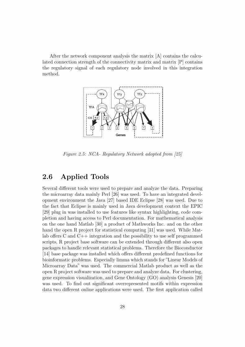
After the network component analysis the matrix [A] contains the calcu-lated connection strength of the connectivity matrix and matrix [P] containsthe regulatory signal of each regulatory node involved in this integrationmethod.

Figure 2.5: NCA- Regulatory Network adopted from [25]

2.6 Applied Tools

Several different tools were used to prepare and analyze the data. Preparingthe microarray data mainly Perl [26] was used. To have an integrated devel-opment environment the Java [27] based IDE Eclipse [28] was used. Due tothe fact that Eclipse is mainly used in Java development context the EPIC[29] plug in was installed to use features like syntax highlighting, code com-pletion and having access to Perl documentation. For mathematical analysison the one hand Matlab [30] a product of Mathworks Inc. and on the otherhand the open R project for statistical computing [31] was used. While Mat-lab offers C and C++ integration and the possibility to use self programmedscripts, R project base software can be extended through different also openpackages to handle relevant statistical problems. Therefore the Bioconductor[14] base package was installed which offers different predefined functions forbioinformatic problems. Especially limma which stands for ”Linear Models ofMicroarray Data” was used. The commercial Matlab product as well as theopen R project software was used to prepare and analyze data. For clustering,gene expression visualization, and Gene Ontology (GO) analysis Genesis [20]was used. To find out significant overrepresented motifs within expressiondata two different online applications were used. The first application called

28

ORA [22] (http://genome.tugraz.at/ORA/) and stands for ”Over representa-tion Analysis” provided by the Institute for Genomics and Bioinformatics atthe University of Technology Graz, Austria. ORA was used with Fisher’s ex-act test as testing and Benjamini and Hochberg as correction settings. Thesecond application called PScan [23] (http://159.149.109.9/pscan/) is alsoan online application to find out overrepresented motifs in expression data.PScan is provided by the Department of Molecular Biology and Biotech-nology at the University of Milan, Italy. PScan was used with z-test astesting and Bonferroni as correction settings. Both applications use the Ref-seq IDs of the expression data to find significant overrepresented motifs ina RefSeq. The BASE application used is provided by Mr. Lei Li Professorat the University of Southern California in Los Angeles. The applicationis available at (http://sites.google.com/site/uscarraylab/research/base). Fi-nally Matlab files for NCA analysis provided by Mr. James C. Liao, Profes-sor at the University of California in Los Angeles, were used. These Matlabfiles are available at (http://www.seas.ucla.edu/˜liaoj/download.htm). Cy-toscape [32] was used for network visualization.

29

Chapter 3

Results

Three different integration methods were used to gather information on themyogenesis process in an early differentiation state. Similar regulatory eventsidentified by all three methods could highlight that this processes may im-portant in the biological context. To show the considerations which weremade prior using these methods the approach is described. The first methodwas clustering and over representation of motifs related to genes which wereallocated to the appropriate cluster due to similar expression behavior overtime. The result of this method was a list of over represented motifs in eachcluster. See appendix A for details. The second method was BASE whichprovided the activity scores of all motifs from the connectivity matrix inconjunction with the expression matrix. As result one can see the temporalbehavior of a motif over all conditions. If a motif does have a relative highpositive activity score under all conditions and its significance q-value is lessthen 0.01 it can be determined that this motif is relatively important for thebiological process. Using this motif now for comparison with the clusteringand over representation results and the same motif can be found in a clusterwith similar expression behavior and is additionally over represented as wellthen it has an obvious significant influence on the biological process, even ifone does not know the exact behavior of the transcription factor’s expres-sion behavior. To proof this consideration the third method called networkcomponent analysis was used to find out if the transcription factor activity(regulatory signal) values calculated by this methods shows a similar behav-ior under all conditions of the expression matrix. If in the NCA analysis thesame motif shows such a behavior it is then even more likely that this tran-scription factor plays a key role on that biological process. After applying allthree methods a list of known transcription factors for that process as wellas some not already assigned transcription factors to that process could bederived.

30

3.1 Co-expressed genes during myogenesis

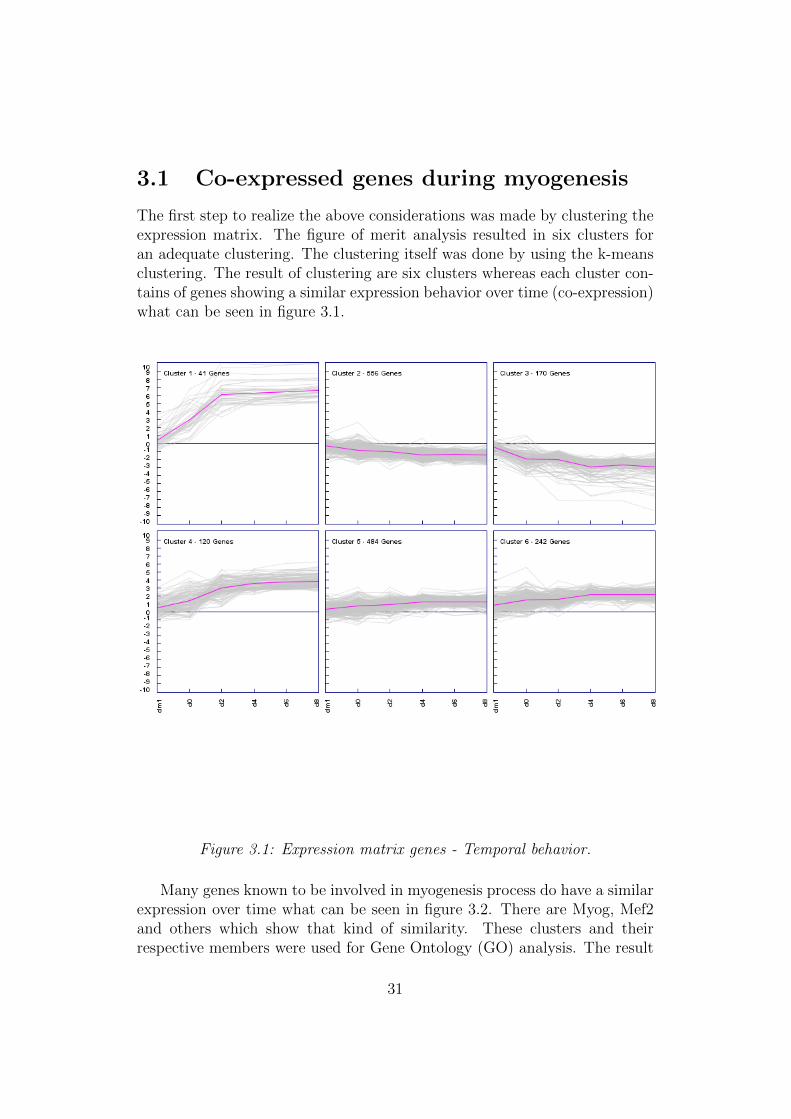
The first step to realize the above considerations was made by clustering theexpression matrix. The figure of merit analysis resulted in six clusters foran adequate clustering. The clustering itself was done by using the k-meansclustering. The result of clustering are six clusters whereas each cluster con-tains of genes showing a similar expression behavior over time (co-expression)what can be seen in figure 3.1.

Figure 3.1: Expression matrix genes - Temporal behavior.

Many genes known to be involved in myogenesis process do have a similarexpression over time what can be seen in figure 3.2. There are Myog, Mef2and others which show that kind of similarity. These clusters and theirrespective members were used for Gene Ontology (GO) analysis. The result

31

Figure 3.2: Similarity of genes in cluster #1.

of GO for the shown cluster can be seen in figure 3.3. The GO distributionof the cluster members having an active behavior evidence their importancein the myogenesis process. The involved genes in that cluster are mainlyinvolved in muscle cell, myoblast, and muscle fiber development. More thanhalf the genes cover these three development areas. According to the activitylevels of all co-expressed genes in cluster number one it is obvious that itsmembers play a key role in myogenesis.

3.2 Over representation

After clustering was finished investigation on over representation was madeusing the online applications Over representation Analysis (ORA) and PScan.For each cluster the Refseq IDs were used as input and as a result ORA andPScan delivered all possible motifs which do have possible binding locationsin the RefSeq IDs provided. The results included several additional informa-tion if a motif is overrepresented identifiable by the calculated p-value. ThePScan online application uses as well the Refseq IDs of the cluster elements.Some additional settings were made to use this application. The organismwas set to mus musculus, the region of interest was set to -950 to +50 base

32

Figure 3.3: Gene Ontology (GO) - Cluster # 1

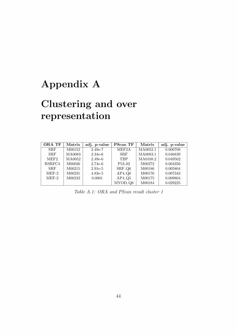
pairs related to the transcription start of the corresponding RefSeq and asdescriptors on the one hand only Jaspar matrices and on the other hand onlyTransfac matrices have been selected. The output of PScan for the clusternumber one can be seen in table 3.1. This application calculated an p-value

ORA TF Matrix adj. p-value PScan TF Matrix adj. p-valueSRF M00152 2.48e-7 MEF2A MA0052.1 0.000708SRF MA0083 2.34e-6 SRF MA0083.1 0.046839

MEF2 MA0052 2.49e-6 TBP MA0108.2 0.049502RSRFC4 M00026 2.74e-6 P53 02 M00272 0.004356

SRF M00215 2.91e-5 SRF Q6 M00186 0.005804MEF-2 M00231 4.83e-5 AP4 Q6 M00176 0.007343MEF-2 M00232 0.0001 AP4 Q5 M00175 0.009804

MYOD Q6 M00184 0.029225

Table 3.1: ORA and PScan result cluster 1

to show an over representation. To get a Bonferroini corrected p-value onecan calculate the adjusted p-value. For that kind of correction it is to mentionthat 130 different Jaspar matrices and 282 Transfac matrices were used. TheJaspar and Transfac over representation results using PScan were arranged inthe same column and apart from the matrix ID the PScan TF value includesan underline symbol followed by additional information. For further com-parison just the transcription factors with an adjusted p-value less then 0.05were used. To show all results of the over representation analysis it is referredto the appendix A. The results show that in the interesting clusters number

33

one, four, five and six some already known transcription factors in contextwith myogenesis are overrepresented as well. In cluster number one MEF2and MyoD are overrepresented. Additionally the serum response factor SRFand the activator protein AP-4 are over represented. There are the tumorsuppressor p53 and the serum response factor related transcription factorRSRFC4 overrepresented as well. Whereas cluster number three, which isthe most down regulated one, includes mainly cell cycle specific transcrip-tion factors over represented like E2F and Elk1. An explanation thereforeis that these cell cycle specific transcription factors are not active after theproliferation. In fact, cluster number three shows cell cycle related genes(e.g. Ccna2, Ccnb2, and Ccnd1) down regulated during the differentiationprocess.

3.3 BASE

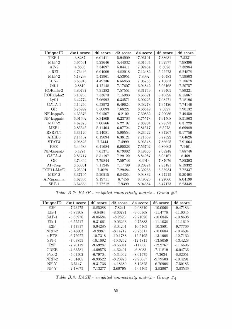
To be able to compare and evaluate the results achieved by the clusteringand over representation step, the binding association with sorted expression(BASE) method was used. The matrices used for that kind of analysis consistof two different connectivity matrices the one with just binary informationand the other with the number of possible binding locations. The dimensionsof the connectivity matrices has been already described in chapter numbertwo. To integrate these data the expression matrix is additionally needed.For each of the 357 motifs representing the binding affinity of the motifin conjunction with the binary matrix as well as the weighted matrix thismethod was applied. Dependent on which connectivity matrix has been usedthis step resulted in two tab delimited files including an activity score for eachcondition in the expression matrix per gene as well as additional informationon the significance of the result. To get an overview on the results theyhave been filtered and only these were analyzed in more detail which hada q-value less than 0.01 at least once over all conditions. 77 motifs usingthe weighted matrix and 78 motifs using the binary matrix in this methodfulfilled the condition. To show the temporal behavior of all interesting motifsthey were grouped depending on their activity scores. Three of the groupsshow considerable activity. Out of the 77 motifs of the weighted connectivitymatrix 63 motifs are active through the differentiation process. The highestactivity at the beginning of the analysis can be seen in group one and two.In these groups there is a significant increase during the first two analyzingdays. The group number three shows a continuous activity of 28 motifs overtime. Active transcription factors are shown in table 3.2. The remainingmotifs in group number four are inactive.

34

Group 1 Group 2 Group 3Srebp1 GATA-3 TEF-1Spz1 CDP MEF-2E47 GATA-2 AP-2

MZF1 GATA-1 c-RELMZF 5-13 MZF 1-4 MEF-2

AP-1 GATA-2 LUN-1RP58 MyoD Olf-1

deltaEF1 Pax-4 RORalfa-2Brachyury Lmo2 RORalpha2

SRF Lyf-1Spz1 GATA-1ER GRSRF NF-kappaB

MyoD NF-kappaBBrachyury MEF-2

E47 MZF1SRF RSRFC4

RUSH1-alfa AREB6AP-4 STAT3HEN1 P300

RREB-1 NF-kappaBSREBP-1 GATA-3

SRF GRMAZR AP-2rep

RREB-1 TCF11-MafGSP1 MEF-2

AP-2gammaSEF-1

Table 3.2: BASE - weighted connectivity matrix - transcription factors

Looking now at the binary connectivity matrix results there is a similarbehavior. Out of 78 interesting motifs also 66 show a significant increase ofactivity. Group number three and number four do have a similar behaviorin comparison with group number one and two of the weighted connectivitymatrix groups. Group two shows a similar behavior as group three of theweighted connectivity matrix group. The inactive motifs of the binary con-nectivity matrix results are shown in group one. Active transcription factorscan be seen in table 3.3. All motifs are shown in the appropriate table andthe activity graphs are shown in the appropriate pictures in appendix B. Thedown regulated group number one using the binary connectivity matrix andgroup number four using the weighted connectivity matrix include cell cyclespecific transcription factors like Elk-1 and E2F which is similar to the overrepresented motifs in cluster number three.

35

Group 2 Group 3 Group 4GATA-1 CDP NF-kappaBMEF2 Srebp1 deltaEF1AP-1 Brachyury NF-kappaBMZF1 MZF 1-4 c-RELAP-4 E47 AP-2rep

AP2alpha HEN1 Pax-4RSRFC4 AP-4 RORalpha2

Ncx HEN1 Lmo2AP-2alpha AP-1 MZF1POU3F2 RREB-1 Lyf-1

NF-kappaB MEF-2 NF-E2Bach1 GR NF-kappaBRoaz SREBP-1 MEF-2Olf-1 SRF SEF-1

NF-kappaB RREB-1 Spz1GATA-3 SP1 SRF

SRF AP-1 AP-2MEF-2 RP58 GR

TCF11-MafG Ik-2 RORalfa-2MyoD MyoD

RUSH1-alfa AREB6ARP-1 MAZR

p65GATA-3GATA-2

Table 3.3: BASE - binary connectivity matrix - transcription factors

3.4 NCA

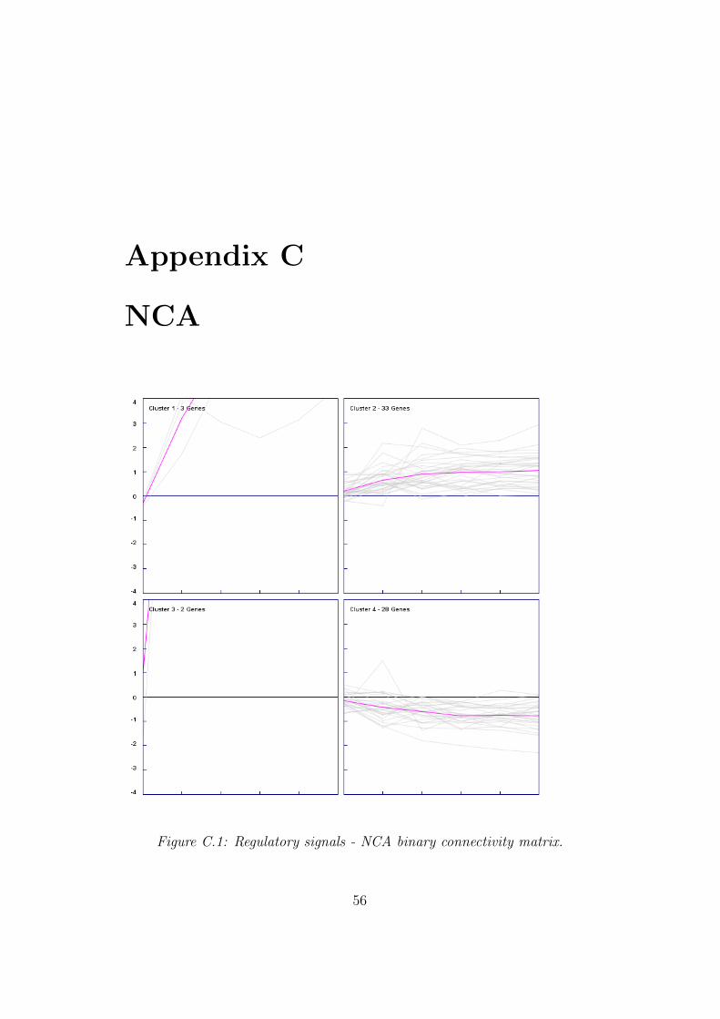
To proof the assumption network component analysis was used to find out ifthe transcription factor activity (regulatory signal) values of the P-matrix ofeach motif can confirm the results of the already applied methods. Thereforetwo new connectivity matrices were generated which included only thesemotifs which have fulfilled the BASE filter criterion. The number of columnsfor the binary connectivity matrix was reduced to 78 and for the weightedconnectivity matrix to 77. Due to the fact that NCA postulates specialmathematical preconditions the matrices were checked for eventually rankdeficiencies and the motifs causing such a deficiency have been removed sothat the number of columns in the binary connectivity matrix was reducedto 66 as well as in the weighted connectivity matrix to 67. The result ofthe network component analysis was also grouped to sort it depending onthe regulatory signals of each motif. Using the binary connectivity matrix

36

NCA showed five motifs which were extremely active at the beginning ofthe analysis which can be seen in the appropriate graph of group one andthree. Group two shows 33 motifs which do have a positive transcriptionfactor activity (TFA) (regulatory signal) value over the complete analyzingprocess. The following table 3.4 shows the motifs with transcription factoractivity (TFA) (regulatory signal). For more details it is referred to appendixC.

Group 1 Group 2 Group 3 Group 1 Group 4MAZR E2F NF-Y NF-kappaB MEF-2MEF2 Spz1 MZF1 MEF-2 CREBAP-2 SRF RP58

HEN1 LUN-1SAP-1 SRFRoaz P300

SREBP-1 TEF-1NF-kappaB MEF-2

MyoD GATA-3E47 NF-Y

MEF-2 SRFPax-4 Pax-4

RUSH1-alfa RUSH1-alfaElk-1 SAP-1AP-1 E2F

GATA-3 RREB-1NF-kappaB MZF1

GR BrachyuryAP-1 SRFSRF c-RELLyf-1 AP-2repMZF1 MyoDRP58 HEN1CDP SRF

GATA-2 RSRFC4MEF-2 Pax-2Olf-1 Spz1

TCF11-MafG ERARP-1 AP-2

E2F MyoDAREB6 AP-1RSRFC4 GATA-2

RORalpha2

Table 3.4: NCA - binary connectivity matrix || weighted connectivity matrix- TFs

Additionally NCA was applied in conjunction with the weighted connec-

37

tivity matrix. Just two motifs show an extremely transcription factor activity(TFA) (regulatory signal) increase at the beginning and 30 motifs show an in-creasing activity over the analysis time line. Table 3.4 shows the transcriptionfactors with positive transcription factor activity (TFA) (regulatory signal)under all conditions as well for the weighted connectivity matrix. All detailedinformation can be found in appendix C.

3.5 Result comparison

Due to the fact that all three methods delivered results which have differ-ent appearances they are compared in this section. The clustering and overrepresentation delivered three interesting clusters in which a specific amountof motifs are overrepresented. As mentioned above the clusters number one,four, five and six show more or less but always positive activities of the genes.Comparing these clusters with the BASE results based on their temporal be-havior cluster number one is first compared with group number three of thebinary connectivity matrix. It can be seen that the known transcription fac-tors like MyoD, Mef2, SRF and AP4 are overrepresented in cluster numberone. The other transcription factors noted in group number two and fourare distributed over the other active clusters number four, five and six. Thisshows that the over represented transcription factors in these clusters showan adequate activity. Furthermore using group number one of the weightedconnectivity matrix which have also a similar temporal behavior as clusternumber one it can bee seen that MyoD, SRF and AP4 are present in thatgroup as well. The transcription factors of group number two and three areas well distributed over the positive active clusters number four, five andsix. This confirms the activity of the overrepresented transcription factorsin BASE analysis. Comparing the NCA results with clusters having similartemporal behavior there are two observations to mention. The first obser-vation is that the grouping of the NCA results led to groups with extremeactivity. These groups include MEF2 in both analyzed connectivity matri-ces. The second observation is that comparing the temporal behavior thematching is not that significant as comparing the BASE results. Further itcould be shown that comparing the NCA binary connectivity matrix resultsof group number two with the active clusters of over representation also in-cludes MyoD, MEF2 , SRF and RSRFC4 which are overrepresented in clusternumber one. The remaining transcripts of group number two are distributedover the other active clusters number four, five and six. A similar distribu-tion of transcripts in group number four was the result of NCA using theweighted connectivity matrix, where MyoD, MEF2, SRF and RSRFC4 over-

38

represented in cluster number one are included in that group. The remainingtranscripts of group number four are distributed over the other active clus-ters number four, five and six. Finally the activity of NFkappaB, not knownas a key player in the myogenesis process, the methods predict that it couldbe involved in this process. It is over represented in cluster number five aswell as active in binary BASE group number two and weighted group num-ber three. In the binary NCA group number four NFkappaB belongs to theactive group and only in the weighted group number four it is not shownas active. In all three methods the appearance of these transcription factorsconcerning the activity and over representation is continuous. Therefore thesignificance of these transcription factors in this biological process led to ahigh probability.

3.6 Gene regulatory network

The overrepresented transcription factors MyoD, Mef2, AP-4, SRF, andRSRFC4 have a connectivity matrix based binding site at the cluster mem-bers of cluster number one and give consistent results over all three integra-tion methods, indicating that these factor are key players of myogenesis [3].At least partly evident also through large scale ChIP on chip studies. Thisbinding situation is illustrated in the following figures. The interaction ofthese transcription factors with the genes is visible due to the color of thenodes representing the genes. Under condition one, see figure 3.4, nearly allgenes are inactive except Rbp1 and Mgp. Over time the activity of the genesis increasing which is illustrated by genes changing the color from green tored, see figure 3.5. The slightly brown and green colored genes are less activethen the red colored genes. At condition four to six all genes in the clustersare active, see figure 3.6, and participate in the myogenesis process.

39

Figure 3.4: Gene regulatory network - condition one

Figure 3.5: Gene regulatory network - condition two

40

Figure 3.6: Gene regulatory network - condition six

41

Chapter 4

Discussion

The applied methods were chosen based on their complementary approachesin analyzing regulatory sequences and gene expression data. Each of themethods has shown its reliability in analyzing these kind of data. Overrepresentation analysis for transcription factor binding sites in co-expressedgenes identifies similar temporal behavior without regarding an explicit bind-ing of transcription factors provided by the connectivity matrices. This factuncouples the result of this method from being much to related to the otheranalyzing methods. The difference in the results of the over representationanalysis by using two different analysis methods illustrates how strong theinfluence is on the method used for in silico prediction of transcription factorbinding sites. In the opposite of word based motif search tools, the biologicalcontext for the construction of position weight matrix for specific transcrip-tion factors is important [33]. Another analysis, over representation of GOterms per cluster could be applied to get additional information on the biolog-ical function of co-expressed genes. BASE and NCA instead use both kindsof data to analyze the biological relationship and importance in this process,but using different approaches. While BASE calculates the results basedon a statistical evaluation to find out the activity of transcription factors,NCA calculates a unique decomposition of the expression data to present ameaningful biological regulatory network. Each of these approaches has itsadvantages. The BASE method uses a straight forward mathematical algo-rithm which results for each transcription factor in an activity score for eachcondition, and applied over several conditions in a time course of the activ-ity score. A variation of BASE was also suggested for gene expression dataand microRNA target prediction [34]. NCA instead uses a more complex ap-proach which results in additional information on the connectivity strengthof the data. The mathematical requirements of NCA are more specific whichleads to a possible loss of information due to these preconditions. NCA was

42

originally applied to E. coli data [10], but was also successfully used in yeastapplications[35] and in mouse [36].

The analyzed data, in more detail the preparation of the data prior analyz-ing must fulfill specific criteria. So the microarray data needed several prepa-ration steps which led to a possible loss of information due to different fil-tering settings and versions of annotations. The reliability of the integrationmethods can be improved by using not only prediction but also using experi-mentally large-scale methods to detect binding sites of transcription factors.Whereas in ChIP-chip TF enrichment regions are identified by hybridizationto promoter elements in ChIP-seq TF binding regions are sequenced and canbe spread over the whole genome. The identified binding regions are shorterwith ChIP-seq and therefore have a better resolution, but it is more difficultto assign a binding site to a specific gene and it is more difficult to constructa connectivity matrix. A solution can be a weighted connectivity matrixnumber of binding sites within a region around the transcription start site( eg. +/- 20kbp) [6] similar used throughout this thesis. Additionally theconstruction of a connectivity matrix is dependent on the used matrices andthe size of the promoter area as well as the settings for finding a possiblebinding location in the promoter area and the used thresholds. Investigatingthe myogenesis process some review papers and articles using high through-put technologies papers have already been published. These publications,e.g. [2] and [3], show similar results like this thesis, in which also MyoD,Myog and MEFs were identified to play a key role in the myogenic differen-tiation process. So the already known transcription factors found during theanalysis in this thesis proof the reliability of the results. The transcriptionfactors, yet not mentioned in this context, which do have similar behaviorand are as well overrepresented such as NFkappaB and MAZR - just to nametwo of them - should be analyzed in more detail to find out if they can beof interest in myogenic differentiation. Finally the usage of three differentmethods for analyzing the myogenesis process confirmed the quality and re-liability of the analyzing methods. Furthermore some transcription factorsnot yet associated with this process could be discovered.

43

Appendix A

Clustering and overrepresentation

ORA TF Matrix adj. p-value PScan TF Matrix adj. p-valueSRF M00152 2.48e-7 MEF2A MA0052.1 0.000708SRF MA0083 2.34e-6 SRF MA0083.1 0.046839

MEF2 MA0052 2.49e-6 TBP MA0108.2 0.049502RSRFC4 M00026 2.74e-6 P53 02 M00272 0.004356

SRF M00215 2.91e-5 SRF Q6 M00186 0.005804MEF-2 M00231 4.83e-5 AP4 Q6 M00176 0.007343MEF-2 M00232 0.0001 AP4 Q5 M00175 0.009804

MYOD Q6 M00184 0.029225

Table A.1: ORA and PScan result cluster 1

44

ORA TF Matrix adj. p-value PScan TF Matrix adj. p-valueMyc-Max MA0059 7.03e-6 HIF1A::ARNT MA0259.1 6.19679e-21

E2F M00516 5.15e-6 E2F1 MA0024.1 6.50338e-21c-Myc:Max M00118 1.42e-5 Arnt::Ahr MA0006.1 1.33842e-18

USF M00217 1.30e-5 MIZF MA0131.1 1.64684e-18ARNT MA0004 8.83e-6 Mycn MA0104.2 3.32027e-17n-MYC MA0104 8.83e-6 GABPA MA0062.2 4.16703e-17NF-Y M00287 1.63e-5 Myc MA0147.1 4.8077e-17USF MA0093 3.34e-5 NFYA MA0060.1 8.73196e-14NF-Y M00185 3.11e-5 ELK4 MA0076.1 2.92622e-12SPI-1 MA0080 9.80e-5 Arnt MA0004.1 1.09637e-11N-Myc M00055 0.0001 Zfx MA0146.1 3.58804e-11c-ETS MA0098 0.0001 SP1 MA0079.2 2.77138e-9E2F M00050 0.0008 Klf4 MA0039.2 4.82186e-9E2F MA0024 0.0007 ELK1 MA0028.1 5.32805e-9

CREB M00178 0.0010 TFAP2A MA0003.1 8.83154e-9USF M00121 0.0029 Egr1 MA0162.1 3.83984e-7E2F M00024 0.0071 MYC::MAX MA0059.1 0.001354

c-Myc:Max M00615 0.0071 USF1 MA0093.1 0.003383Arnt M00236 0.0072 ETS1 MA0098.1 0.003469Max MA0058 0.0076 Pax5 MA0014.1 0.016896

CRE-BP1 M00179 0.0092 E2F 03 M00516 4.24554e-33Sp1 M00196 0.0088 E2F 02 M00050 6.70977e-22

NRSF M00256 0.0088 SP1 Q6 M00196 4.88929e-21Max M00119 0.0087 AP2 Q6 M00189 1.44327e-18USF M00187 0.0149 NFY 01 M00287 1.54219e-13

NRF-2 M00108 0.0175 SP1 01 M00008 1.28888e-10NRF-2 MA0062 0.0175 NMYC 01 M00055 1.50819e-9

Tax/CREB M00114 0.0465 ELK1 02 M00025 7.27656e-9

Table A.2: ORA and PScan result cluster 2 - Part1

45

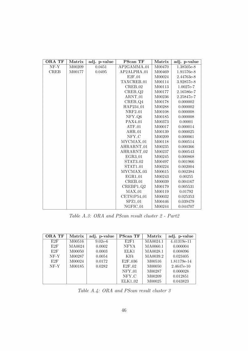
ORA TF Matrix adj. p-value PScan TF Matrix adj. p-valueNF-Y M00209 0.0451 AP2GAMMA 01 M00470 1.38505e-8CREB M00177 0.0495 AP2ALPHA 01 M00469 1.91576e-8

E2F 01 M00024 2.44763e-8TAXCREB 01 M00114 3.92857e-8

CREB 02 M00113 1.0027e-7CREB Q2 M00177 2.16586e-7ARNT 01 M00236 2.25847e-7CREB Q4 M00178 0.000002

HAP234 01 M00288 0.000002NRF2 01 M00108 0.000008NFY Q6 M00185 0.000008PAX4 01 M00373 0.00001ATF 01 M00017 0.000014AHR 01 M00139 0.000025NFY C M00209 0.000061

MYCMAX 01 M00118 0.000514AHRARNT 01 M00235 0.000366AHRARNT 02 M00237 0.000543

EGR3 01 M00245 0.000868STAT3 02 M00497 0.001966STAT1 01 M00224 0.002004

MYCMAX 03 M00615 0.002384EGR1 01 M00243 0.00255CREB 01 M00039 0.004167

CREBP1 Q2 M00179 0.005531MAX 01 M00119 0.01792

CETS1P54 01 M00032 0.025353SPZ1 01 M00446 0.039479

NGFIC 01 M00244 0.044707

Table A.3: ORA and PScan result cluster 2 - Part2

ORA TF Matrix adj. p-value PScan TF Matrix adj. p-valueE2F M00516 9.02e-6 E2F1 MA0024.1 4.41319e-11E2F MA0024 0.0002 NFYA MA0060.1 0.000004E2F M00050 0.0003 ELK1 MA0028.1 0.008096

NF-Y M00287 0.0054 Klf4 MA0039.2 0.023405E2F M00024 0.0172 E2F 036 M00516 1.81179e-14

NF-Y M00185 0.0282 E2F 02 M00050 2.4647e-10NFY 01 M00287 0.000028NFY C M00209 0.012851

ELK1 02 M00025 0.043823


46

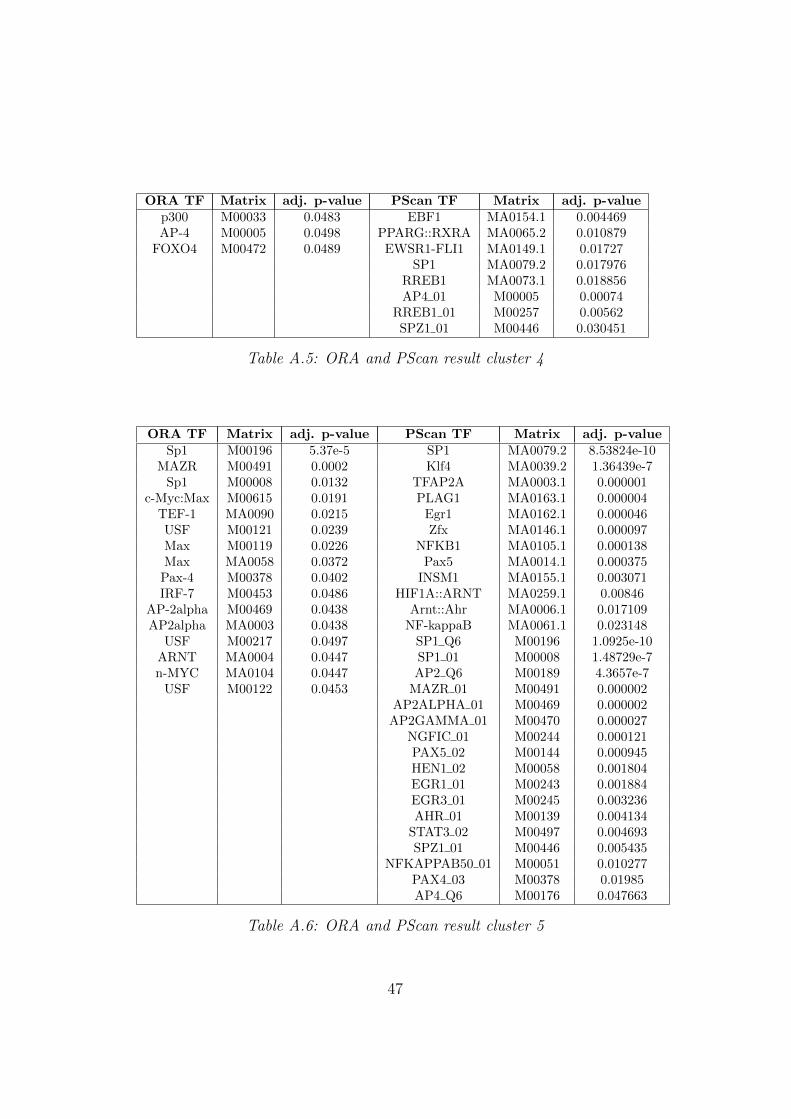
ORA TF Matrix adj. p-value PScan TF Matrix adj. p-valuep300 M00033 0.0483 EBF1 MA0154.1 0.004469AP-4 M00005 0.0498 PPARG::RXRA MA0065.2 0.010879

FOXO4 M00472 0.0489 EWSR1-FLI1 MA0149.1 0.01727SP1 MA0079.2 0.017976

RREB1 MA0073.1 0.018856AP4 01 M00005 0.00074

RREB1 01 M00257 0.00562SPZ1 01 M00446 0.030451


ORA TF Matrix adj. p-value PScan TF Matrix adj. p-valueSp1 M00196 5.37e-5 SP1 MA0079.2 8.53824e-10

MAZR M00491 0.0002 Klf4 MA0039.2 1.36439e-7Sp1 M00008 0.0132 TFAP2A MA0003.1 0.000001

c-Myc:Max M00615 0.0191 PLAG1 MA0163.1 0.000004TEF-1 MA0090 0.0215 Egr1 MA0162.1 0.000046USF M00121 0.0239 Zfx MA0146.1 0.000097Max M00119 0.0226 NFKB1 MA0105.1 0.000138Max MA0058 0.0372 Pax5 MA0014.1 0.000375

Pax-4 M00378 0.0402 INSM1 MA0155.1 0.003071IRF-7 M00453 0.0486 HIF1A::ARNT MA0259.1 0.00846

AP-2alpha M00469 0.0438 Arnt::Ahr MA0006.1 0.017109AP2alpha MA0003 0.0438 NF-kappaB MA0061.1 0.023148

USF M00217 0.0497 SP1 Q6 M00196 1.0925e-10ARNT MA0004 0.0447 SP1 01 M00008 1.48729e-7n-MYC MA0104 0.0447 AP2 Q6 M00189 4.3657e-7

USF M00122 0.0453 MAZR 01 M00491 0.000002AP2ALPHA 01 M00469 0.000002

AP2GAMMA 01 M00470 0.000027NGFIC 01 M00244 0.000121PAX5 02 M00144 0.000945HEN1 02 M00058 0.001804EGR1 01 M00243 0.001884EGR3 01 M00245 0.003236AHR 01 M00139 0.004134

STAT3 02 M00497 0.004693SPZ1 01 M00446 0.005435

NFKAPPAB50 01 M00051 0.010277PAX4 03 M00378 0.01985AP4 Q6 M00176 0.047663


47

ORA TF Matrix adj. p-value PScan TF Matrix adj. p-valuePPARG M00515 0.0427 Klf4 MA0039.2 0.002396HEN1 M00058 0.0359 SP1 MA0079.2 0.007252

Zfx MA0146.1 0.019163TFAP2A MA0003.1 0.025848SP1 Q6 M00196 0.001434

MAZR 01 M00491 0.010193


48

Appendix B

BASE

Figure B.1: Temporal behavior - BASE - binary connectivity matrix

49

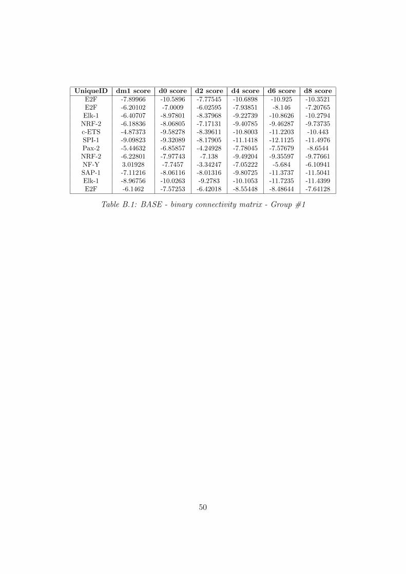
UniqueID dm1 score d0 score d2 score d4 score d6 score d8 scoreE2F -7.89966 -10.5896 -7.77545 -10.6898 -10.925 -10.3521E2F -6.20102 -7.0009 -6.02595 -7.93851 -8.146 -7.20765Elk-1 -6.40707 -8.97801 -8.37968 -9.22739 -10.8626 -10.2794

NRF-2 -6.18836 -8.06805 -7.17131 -9.40785 -9.46287 -9.73735c-ETS -4.87373 -9.58278 -8.39611 -10.8003 -11.2203 -10.443SPI-1 -9.09823 -9.32089 -8.17905 -11.1418 -12.1125 -11.4976Pax-2 -5.44632 -6.85857 -4.24928 -7.78045 -7.57679 -8.6544NRF-2 -6.22801 -7.97743 -7.138 -9.49204 -9.35597 -9.77661NF-Y 3.01928 -7.7457 -3.34247 -7.05222 -5.684 -6.10941SAP-1 -7.11216 -8.06116 -8.01316 -9.80725 -11.3737 -11.5041Elk-1 -8.96756 -10.0263 -9.2783 -10.1053 -11.7235 -11.4399E2F -6.1462 -7.57253 -6.42018 -8.55448 -8.48644 -7.64128

Table B.1: BASE - binary connectivity matrix - Group #1

50

Figure B.2: Temporal behavior - BASE - weighted connectivity matrix

51

UniqueID dm1 score d0 score d2 score d4 score d6 score d8 scoreGATA-1 3.71003 4.71561 4.66048 7.07699 6.63536 6.59123MEF2 4.02625 4.22286 5.27628 7.52533 6.71043 6.97343AP-1 4.13693 7.99204 4.70046 6.65458 5.97127 5.44146MZF1 3.00575 4.82563 6.31421 7.74828 6.54684 6.57308AP-4 2.46471 7.3136 4.78455 5.89874 6.02971 5.87792

AP2alpha 3.24335 7.40828 4.39911 6.30337 6.0494 6.41436RSRFC4 3.3264 4.3497 5.68576 7.43935 6.28113 6.43242

Ncx 2.05679 7.74867 4.17729 6.56169 5.61332 5.60558AP-2alpha 3.29622 7.54417 4.42032 6.39252 6.13376 6.44723POU3F2 6.03883 7.71605 3.41268 4.49424 3.8374 3.76471

NF-kappaB 4.16874 6.69821 5.29528 7.02003 6.03998 6.87388Bach1 2.44649 7.26745 4.80244 6.19758 4.75928 4.53717Roaz 2.30646 6.12735 6.99575 6.29435 5.96542 6.24186Olf-1 2.12901 4.90148 7.06081 7.10272 6.84254 6.98112

NF-kappaB 2.30348 6.96753 6.2746 7.16749 6.55889 7.12597GATA-3 2.96499 4.20172 5.83273 8.20749 7.41858 7.1485

SRF 3.47025 6.78588 7.16037 6.43869 6.81095 6.68771MEF-2 4.45103 6.53085 5.25031 7.02289 7.50175 7.5972

TCF11-MafG 3.49426 5.21459 5.80344 7.36513 7.06837 6.48535


UniqueID dm1 score d0 score d2 score d4 score d6 score d8 scoreCDP -2.37242 7.27366 8.92312 7.86707 8.73393 7.8817

Srebp1 -2.54048 6.81913 8.30249 6.9586 7.37683 7.44478Brachyury -3.52707 4.55542 6.59235 7.12036 6.68123 7.195MZF 1-4 -2.40183 8.00813 6.65178 9.29554 8.21077 8.17662

E47 -3.018 3.91652 7.58454 7.45715 6.82153 7.5754HEN1 -2.73043 6.62514 5.1873 6.92221 6.11376 6.11301AP-4 -1.40265 5.26184 6.00745 7.71622 7.24001 7.25966HEN1 -2.34257 7.30034 4.89938 6.91436 5.96177 6.04766AP-1 -2.72032 7.33242 4.30264 6.12195 5.67222 4.81493

RREB-1 -2.93415 4.68311 7.472 6.72728 6.74344 7.1014MEF-2 -2.44536 4.84328 6.01394 8.28651 7.58517 7.54277

GR -2.77277 4.01632 7.69994 7.46543 6.56816 7.62039SREBP-1 -4.30836 5.89683 6.42508 6.46239 6.5622 7.39713

SRF -2.74186 3.21393 6.89948 6.4845 7.46541 7.27247RREB-1 -2.83198 7.64045 7.64326 9.11583 9.23529 10.2841

SP1 -4.2011 8.20657 7.00235 7.92192 7.34988 7.89754AP-1 -3.00128 6.90599 7.41885 6.25638 6.24942 6.6469RP58 -2.38893 7.03001 5.77989 8.14324 6.87287 7.4251Ik-2 -2.84559 5.76735 6.40369 6.88055 5.66867 6.9965

MyoD -3.81412 4.11256 9.37843 7.54972 7.65486 8.00769RUSH1-alfa -2.54926 6.4972 7.14237 8.2615 8.87522 8.94101

ARP-1 -1.6468 6.17796 5.8244 6.39409 6.58392 6.98897


52

UniqueID dm1 score d0 score d2 score d4 score d6 score d8 scoreNF-kappaB 4.16925 7.46701 6.48906 8.89672 8.09268 8.67314deltaEF1 1.86107 6.59636 9.11186 8.61119 7.47706 8.47199

NF-kappaB 3.39506 7.83908 7.35357 7.80075 6.47559 7.49485c-REL 5.58583 7.48233 6.03831 7.98966 6.50216 7.56524

AP-2rep 2.58563 6.87171 6.41782 8.3806 7.80102 7.99881Pax-4 3.51923 10.6276 8.64834 11.0514 9.81632 11.0176

RORalpha2 4.74964 7.08901 7.32557 8.786 7.9298 8.03634Lmo2 2.817 7.85156 8.38016 9.23447 8.08581 8.54932MZF1 2.4485 7.11671 6.65151 7.96263 7.48427 7.52468Lyf-1 3.12127 8.11446 7.47662 8.52834 8.08017 8.19262

NF-E2 4.75924 9.03288 8.47293 8.36563 8.40209 8.30895NF-kappaB 2.79765 8.28746 6.54063 7.72394 7.23982 7.84809

MEF-2 5.89661 7.63149 6.85065 9.01182 8.42779 8.19488SEF-1 3.98412 8.95752 7.26778 8.09604 7.63907 7.83918Spz1 2.15206 7.8025 6.92858 7.32221 6.84946 6.88369SRF 4.40492 7.54407 6.49638 8.78913 8.53908 7.82608AP-2 4.22712 7.82555 5.80921 7.22908 7.03918 7.98433GR 3.93024 8.20042 6.04038 7.74953 7.27195 6.90328

RORalfa-2 4.9621 7.07192 7.99814 8.33935 7.8415 7.67969MyoD 2.86503 7.13745 8.87418 8.6028 8.53497 8.40198

AREB6 3.16549 6.41168 7.36033 8.0167 7.52691 7.60346MAZR 2.64547 8.1659 7.45832 9.20705 8.14513 8.99485

p65 4.38337 7.61155 6.82277 7.87021 6.60913 7.88171GATA-3 2.97356 8.2377 7.18177 8.48224 7.92371 7.90245GATA-2 3.12814 8.71333 7.15698 9.44223 8.8263 8.81989


53

UniqueID dm1 score d0 score d2 score d4 score d6 score d8 scoreSrebp1 -3.27174 6.14126 7.94301 6.73534 6.96341 7.32519Spz1 -2.0509 7.04195 8.10684 8.73398 8.49699 8.28223E47 -4.38291 3.65562 6.02747 6.49127 5.73575 7.31434

MZF1 -4.13172 6.46696 6.08531 7.19671 6.87955 6.65818MZF 5-13 -2.38503 7.60384 6.26635 7.69925 7.60839 7.42655

AP-1 -3.80379 4.67992 7.70028 5.33648 6.22443 6.42832RP58 -2.52837 6.23608 5.49711 7.17248 6.07548 6.41804

deltaEF1 -2.48403 7.40212 8.00545 9.136 8.23111 9.23549Brachyury -3.90106 3.61963 6.32025 7.16915 7.12887 6.88777

SRF -2.86987 5.25737 7.31268 7.26274 6.71243 6.34417Spz1 -2.63391 7.59554 8.22961 9.42421 8.688 9.28323ER -2.61902 6.35706 7.71628 7.73863 6.9513 7.11424SRF -3.31282 8.09296 9.17011 10.3098 9.99244 9.60908

MyoD -2.98676 5.15316 9.5694 8.61478 9.09106 9.37964Brachyury -2.08929 5.64264 5.87305 7.43788 6.53318 6.25188

E47 -2.47516 4.54581 7.29201 8.12914 7.95062 8.61648SRF -4.18286 6.02343 8.9065 9.01961 8.52681 8.66441

RUSH1-alfa -2.48779 8.36898 7.67173 10.2481 10.3388 10.1936AP-4 -1.47037 5.10128 6.29696 7.27167 7.4087 7.4267HEN1 -2.8087 8.39257 6.24505 8.38458 6.78173 7.49811

RREB-1 -2.62761 7.30048 7.96423 8.92056 8.5171 9.24014SREBP-1 -4.26832 7.39692 8.39755 7.88483 8.06307 8.94048

SRF -2.65144 4.99047 8.0417 8.5029 8.80198 8.55637MAZR -2.531 9.85543 6.78409 9.58544 8.20701 9.14196

RREB-1 -4.05456 6.99743 7.1608 7.91298 7.52696 8.63929SP1 -3.41026 9.6347 9.75557 10.3028 9.25748 10.0863

Table B.5: BASE - weighted connectivity matrix - Group #1

UniqueID dm1 score d0 score d2 score d4 score d6 score d8 scoreGATA-3 5.06903 8.61463 7.44072 9.56069 8.3126 9.00447

CDP 3.04632 7.46112 9.25316 8.11846 9.27168 8.68494GATA-2 4.78266 8.09901 7.62026 9.97959 9.19675 8.82802GATA-1 2.29342 8.45931 10.2539 10.8778 10.1413 10.4455MZF 1-4 3.03039 11.7641 10.548 13.2464 11.8181 13.0315GATA-2 5.26485 9.17549 6.73649 10.1724 8.80166 8.88388MyoD 2.94338 8.94521 10.5675 10.7985 10.473 10.7466Pax-4 3.58007 11.0146 10.0488 12.1434 10.8706 11.7259Lmo2 2.74458 7.51592 8.82359 9.41741 8.92893 9.51133


54

UniqueID dm1 score d0 score d2 score d4 score d6 score d8 scoreTEF-1 3.8287 6.01411 5.94909 7.96191 7.38631 7.5231MEF-2 3.65531 5.23646 5.44032 8.61634 7.92977 7.98396AP-2 4.8508 7.34697 5.04411 7.02454 6.5028 7.38984c-REL 4.73446 6.94009 4.82918 7.12482 5.22273 6.24878MEF-2 5.18293 5.43961 4.53951 7.8092 6.46483 7.59803LUN-1 3.53913 4.49736 6.55853 7.05756 7.10653 7.18678Olf-1 2.8819 4.12148 7.17607 6.94842 5.96168 7.20757

RORalfa-2 4.80737 7.31282 7.57551 8.31749 8.39405 7.89221RORalpha2 5.10255 7.33673 7.15983 8.65321 8.40828 8.15867

Lyf-1 3.42774 7.96992 6.34571 6.90225 7.08271 7.18196GATA-1 3.14246 6.53972 6.49624 9.38278 7.35126 7.74146

GR 3.76992 5.50093 7.68221 8.68649 7.3827 7.90132NF-kappaB 4.35376 7.91507 6.2102 7.50832 7.20086 7.49459NF-kappaB 6.01692 8.34809 6.23703 8.75578 7.91508 8.51863

MEF-2 4.67873 7.06566 5.22107 7.83904 7.28523 6.31229MZF1 2.85545 5.11404 6.07724 7.81517 6.5278 6.69989

RSRFC4 3.33126 5.14081 5.90554 9.23422 8.37267 9.17756AREB6 2.14467 6.19094 6.38121 7.71659 6.77522 7.64626STAT3 2.96825 7.7444 7.4999 6.93548 7.86625 7.91064P300 3.44683 6.41684 6.90028 7.56702 6.86663 7.1461

NF-kappaB 5.4274 7.61371 6.79082 8.49866 7.08248 7.88746GATA-3 2.85717 5.51197 7.29122 8.84987 8.05167 8.469

GR 3.74364 7.79844 7.59748 8.3913 7.87076 7.85393AP-2rep 3.50031 7.11245 7.17789 9.20874 7.83181 8.19332

TCF11-MafG 3.25391 7.4029 7.29484 8.39258 8.33934 7.72337MEF-2 3.37195 5.20515 6.84384 9.94832 8.47215 9.30498

AP-2gamma 4.62805 9.19711 6.7456 8.49026 7.27066 8.04199SEF-1 3.54663 7.77212 7.9399 8.04684 8.47173 8.23348


UniqueID dm1 score d0 score d2 score d4 score d6 score d8 scoreE2F -7.23275 -8.85288 -7.8241 -9.98319 -10.0068 -9.47183Elk-1 -5.89308 -8.8464 -8.66781 -9.66368 -11.4778 -11.0045SAP-1 -5.65976 -8.05584 -8.2823 -9.71028 -10.6845 -10.8608Elk-1 -6.55517 -9.31661 -9.06263 -9.75883 -11.1038 -11.1619E2F -7.47317 -8.94285 -8.04201 -10.5463 -10.3891 -9.77766

NRF-2 -5.48803 -8.9987 -8.14717 -9.73511 -10.0684 -10.4594c-ETS -6.72927 -10.7318 -10.1788 -12.5195 -13.1908 -12.7162SPI-1 -7.63855 -10.1092 -10.6262 -12.4811 -13.8059 -13.4228E2F -7.70119 -9.59287 -8.66041 -11.656 -12.2767 -11.5696

CREB -4.63581 -4.09576 -4.62491 -6.8083 -7.11819 -6.04736Pax-2 -5.67502 -6.79704 -5.34042 -8.01575 -7.3634 -8.82051NRF-2 -5.51405 -8.93522 -8.23978 -9.95057 -9.79503 -10.4291NF-Y 3.5147 -9.31736 -4.18689 -8.12825 -6.70908 -7.50185NF-Y -2.18675 -7.13277 2.69795 -4.04765 -2.92907 -3.83536


55

Appendix C

NCA

Figure C.1: Regulatory signals - NCA binary connectivity matrix.

56

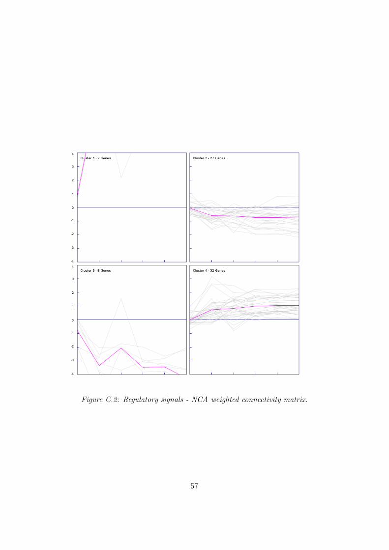
Figure C.2: Regulatory signals - NCA weighted connectivity matrix.

57

UniqueID dm1 int. d0 int. d2 int. d4 int. d6 int. d8 int.MAZR -0.18359 4.1076 3.0428 2.3867 3.1384 4.4844MEF2 -0.41377 1.7148 4.9437 5.0224 4.1613 4.3558AP-2 -0.27525 3.7242 9.6006 5.0036 5.7799 4.9551

Table C.1: NCA - binary connectivity matrix - Group #1

UniqueID dm1 int. d0 int. d2 int. d4 int. d6 int. d8 int.E2F 0.91434 0.91344 0.55512 0.39632 1.3072 1.2022Spz1 -0.22442 0.52342 0.082821 0.30352 0.28334 0.10403SRF 0.36508 0.91385 0.27732 0.59557 0.7514 0.84402

HEN1 0.16797 0.56008 -0.12302 0.099718 0.28599 0.31141SAP-1 0.01456 0.52322 0.58318 0.27753 0.59489 0.18853Roaz -0.059423 0.56315 -0.02058 -0.047733 0.32915 0.26371

SREBP-1 0.32628 0.47213 0.58827 0.19818 0.39008 0.36087NF-kappaB 0.53391 0.90123 0.28931 0.616 0.39642 0.31952

MyoD 0.13696 0.53568 0.41263 0.38371 0.0054716 -0.053514E47 0.081694 0.66458 0.32892 0.85363 0.43685 0.48403

MEF-2 0.15857 0.15831 1.0286 0.3389 0.62696 0.52143Pax-4 0.1972 0.038074 0.52751 0.67651 0.39255 0.7734

RUSH1-alfa -0.075259 0.33221 0.77391 1.1318 0.7735 0.63978Elk-1 0.089314 0.41786 0.63983 0.30894 0.60961 0.57304AP-1 0.31245 0.1109 1.0553 0.91587 0.94181 0.8031

GATA-3 -0.22824 0.2992 1.0302 1.1059 0.9014 0.83927NF-kappaB 0.17176 0.23912 0.55832 0.99575 0.81538 1.2583

GR 0.15782 0.27895 0.84866 1.1665 1.3508 1.5838AP-1 0.012139 0.069373 0.544 1.0926 0.95127 1.0447SRF 0.59502 0.41228 1.0132 1.2458 1.1832 1.2459Lyf-1 0.6696 1.3665 0.89837 1.0538 1.3597 1.3378MZF1 -0.047636 1.0704 0.60882 1.1981 1.275 1.3407RP58 0.028363 0.2076 0.75111 1.0792 0.99821 1.3495CDP -0.003986 1.0289 1.2313 1.0721 1.103 0.99556

GATA-2 0.17937 1.7559 1.1138 1.4887 1.3119 1.2446MEF-2 0.51157 0.89665 1.3592 1.2952 1.3536 1.5174Olf-1 0.87875 0.87617 0.93203 1.3175 1.4469 1.592

TCF11-MafG -0.043055 0.83898 2.1562 1.7354 1.6185 1.5501ARP-1 0.077484 0.45333 1.6928 1.7795 1.8424 1.8976

E2F 0.18799 1.1948 1.5266 1.9635 1.8011 2.1192AREB6 0.60793 0.80683 1.4733 1.5789 1.7448 1.7711RSRFC4 -0.038575 2.1732 2.0163 1.7231 1.5585 1.6627

RORalpha2 -0.18667 -0.39531 2.7877 2.0887 2.2854 2.9258


58

UniqueID dm1 int. d0 int. d2 int. d4 int. d6 int. d8 int.NF-Y -1.8363 22.831 14.408 25.761 20.656 25.592MZF1 3.723 17.604 18.995 33.144 28.732 29.325


UniqueID dm1 int. d0 int. d2 int. d4 int. d6 int. d8 int.MEF-2 -0.38076 -0.54717 -0.25093 -0.86213 -0.72655 -0.56727

GATA-1 -0.03448 -0.42655 -1.0626 -1.0772 -1.012 -1.1841RREB-1 -0.3657 -1.1969 -0.91159 -0.81588 -0.97001 -1.0574

Ncx -0.027488 -0.73866 -0.18441 -0.74532 -0.72994 -0.603Brachyury 0.36293 -0.24769 -0.74674 -0.83891 -0.54656 -0.81424

Elk-1 -0.23351 -0.40422 -0.75573 -1.0609 -0.90935 -1.3436Ik-2 -0.091641 -0.70852 -0.45782 -0.55572 -0.2376 -0.36577

HEN1 -0.27611 -1.1972 -1.7777 -1.989 -2.1605 -2.2802Lmo2 0.10905 -0.69446 -0.58358 -0.6619 -0.8647 -0.74137

RREB-1 -0.36812 -0.22724 -0.82932 -0.74066 -0.79343 -0.58775NF-E2 0.13603 0.19869 -0.39702 -0.20291 -0.4234 -0.15783

GR -0.51395 -0.28286 -0.0075441 -0.32181 -0.35916 -0.024366NF-kappaB -0.66981 -0.42939 -0.22091 -0.19182 -0.45433 -0.19257

SRF 0.19479 0.088349 -0.62679 -0.40903 -0.38817 -0.74109SP1 -0.41323 1.501 -1.3571 -0.78803 -1.2058 -0.27501AP-4 -0.12456 -0.17643 -0.62456 -0.35134 -0.73562 -0.42245AP-1 -0.66552 -0.43369 -0.32562 -0.73289 -0.86942 -1.0133Pax-2 -0.30133 -1.0398 -1.2721 -1.3023 -1.3618 -1.5758Srebp1 -0.2562 -1.2702 -0.5802 -1.2892 -1.2202 -1.503SEF-1 -0.29334 -0.64827 -1.0565 -0.72927 -0.87776 -1.0512c-REL -0.6261 -0.50999 -1.0505 -1.0054 -1.2351 -1.3284Bach1 0.061449 -0.30877 -0.58014 -1.3472 -0.65647 -1.0186

GATA-3 0.091425 0.2248 -0.068894 -0.37556 -0.47415 -0.40685AP-2rep -0.12859 -0.65207 -0.40118 -0.99122 -0.68998 -0.93696MyoD -0.20273 -0.86627 0.030423 -0.41089 -0.46454 -0.45223AP-4 0.3151 -0.97178 -0.58791 -0.98314 -0.72079 -0.9304

NF-kappaB 0.20588 0.17061 -0.34983 -0.24582 -0.089356 0.081519p65 0.49724 0.14724 0.0061475 -0.19866 0.28177 0.10698


UniqueID dm1 int. d0 int. d2 int. d4 int. d6 int. d8 int.NF-kappaB 1.1082 9.0572 2.1735 6.1039 5.2897 7.2798

MEF-2 0.63646 8.6266 8.1705 8.6895 8.6835 8.4819

Table C.5: NCA - weighted connectivity matrix - Group #1

59

UniqueID dm1 int. d0 int. d2 int. d4 int. d6 int. d8 int.STAT3 -0.061278 -0.77677 -0.27397 -0.21541 -0.086855 0.073754Elk-1 -0.018571 -0.22095 -0.16878 0.040882 -0.25169 -0.27567AP-4 -0.070574 0.35296 -0.43804 -0.19248 -0.48927 -0.57169Lmo2 0.37587 0.51045 -0.41625 -0.46307 -0.53288 -0.68566Elk-1 0.050081 -0.25386 -0.76 -0.62596 -0.72032 -0.68127MZF1 0.2076 -1.1749 -0.16658 -0.40349 -0.64699 -0.51236

MZF 5-13 0.39389 0.011905 0.029392 -0.33244 0.041387 0.15656AP-2gamma 1.0739 -0.61315 -0.89285 -1.4768 -0.59213 -1.0189

GR -0.45458 -0.8187 0.29082 -0.32019 -0.51563 -0.25566SREBP-1 -0.17671 0.12266 -0.61199 -0.73821 -0.71496 -0.94965RREB-1 0.071703 -0.94714 -0.20001 0.12605 -0.25874 -0.07663

SP1 -0.50924 -0.83223 -0.62503 -0.69177 -0.54162 -0.55079CDP -0.61055 -0.92335 -0.27133 -0.41747 -0.47442 -0.55149

AREB6 -0.17028 -0.67383 -0.68677 -0.64398 -0.48453 -0.89469Olf-1 -0.59334 -0.91808 -0.56892 -1.1938 -1.1577 -1.2625

NF-kappaB NaN -0.17625 -0.41052 -0.688 -1.2426 -0.98612NF-Y -0.14723 -0.80533 -0.28394 -0.99185 -0.94424 -1.2269GR 0.46579 -0.14799 -0.44498 8.0436E-4 0.094355 0.17136

Brachyury -0.1898 -1.1186 -0.47857 -1.0746 -1.0975 -0.41329GATA-1 -0.47495 -0.70654 -1.1526 -1.4971 -1.6856 -1.7671Srebp1 -0.31625 -1.568 -0.71619 -1.5914 -1.5062 -1.8552Spz1 -0.17898 -0.05208 -0.41188 0.086424 0.075674 0.35747

SEF-1 -0.0025944 -1.198 -1.4571 -1.6097 -1.5636 -1.9707E47 -0.17637 -1.6379 -1.1302 -1.5003 -1.4075 -1.6166E47 0.072135 -0.57852 -1.7088 -1.929 -1.9788 -1.8262

Lyf-1 0.82392 -0.21775 -1.8636 -0.037459 0.81001 0.78113MEF-2 -0.38894 -0.99776 -1.1131 -1.9615 -1.915 -2.1897


UniqueID dm1 int. d0 int. d2 int. d4 int. d6 int. d8 int.MAZR 0.13875 -3.8544 -4.2862 -6.0198 -4.7844 -9.6023

NF-kappaB -1.9317 -5.8358 -2.1372 -3.8403 -3.7626 -4.6579E2F 0.13091 -2.5423 -1.7524 -1.9765 -2.6647 -2.1897

GATA-3 -0.21561 -3.1526 -3.686 -3.0498 -2.838 -2.026RORalpha2 -0.70143 -2.0285 -2.0598 -2.916 -3.412 -3.6612

TCF11-MafG -1.9552 -2.7535 1.5488 -3.0854 -3.1986 -3.6158


60

UniqueID dm1 int. d0 int. d2 int. d4 int. d6 int. d8 int.MEF-2 0.55707 0.7542 -0.67583 0.53137 0.42688 0.84397CREB 0.044928 0.59746 -0.37759 0.29331 0.063407 0.14702RP58 -0.19013 -0.1224 0.3987 0.57188 0.79257 0.92316LUN-1 -0.12364 0.42713 0.73723 0.21872 0.59981 0.66032SRF 0.21667 -0.021332 0.55573 0.8108 1.0154 0.78644P300 -0.32338 -0.31602 0.98961 0.21513 0.55842 0.72992

TEF-1 -0.26477 -0.16161 0.24793 0.52332 0.61836 0.3707MEF-2 -0.20065 1.5451 -0.81011 0.32791 0.45459 -0.0050765

GATA-3 -0.28077 0.71564 0.193 0.50233 0.9789 0.92827NF-Y 0.19095 0.28048 0.85275 1.1754 1.1237 0.80035SRF -0.21024 -0.19129 0.80636 0.45984 0.65887 0.42244

Pax-4 0.72707 0.37752 1.5272 0.97756 0.82933 0.72302RUSH1-alfa -0.17358 0.76798 -0.13045 0.59529 0.4076 0.52822

SAP-1 -0.044558 0.99996 0.59878 0.66867 0.62453 0.72989E2F -0.052023 0.79724 0.51634 0.42695 0.70081 0.36771

RREB-1 -0.24712 0.21801 0.3951 0.41995 0.61737 0.6738MZF1 -0.21702 -0.26099 0.84607 0.32106 0.64458 0.36939

Brachyury -0.67031 0.16655 0.32038 -0.053525 0.19868 0.10105SRF -0.048934 0.42763 1.4801 1.4112 1.7838 1.6078

c-REL -0.077502 0.28377 1.0328 1.227 0.88971 1.0383AP-2rep -0.34238 0.82191 1.4217 1.3156 1.268 1.3292MyoD -0.11467 1.0981 0.93642 1.1565 1.4416 1.4186HEN1 0.12362 0.38045 1.0476 1.6269 1.3712 1.4477SRF -0.041273 0.5643 1.7367 1.5056 1.6201 1.7965

RSRFC4 0.55333 0.78743 1.0105 1.8248 1.512 1.8692Pax-2 -0.016473 1.183 1.3374 1.7177 1.5884 2.223Spz1 -0.33433 0.64992 1.4068 1.6641 1.6692 1.6677ER -0.088758 1.2755 1.2427 1.6121 1.6338 1.9629

AP-2 0.97819 2.6291 2.5143 1.7591 1.7645 1.6223MyoD 0.053267 1.2335 1.5595 2.2487 2.2256 2.2745AP-1 -0.010668 3.1807 1.9971 2.07 1.9349 1.843

GATA-2 0.31276 2.5709 1.4911 2.2228 1.8368 1.7152


61

Bibliography

[1] Sabourin L.A. and Rudnicki M.A. The molecular regulation ofmyogenesis. Clinical Genetics, 57:16–25, 2000.

[2] Tomczak K.K., Marinescu V.D., et al. Expression profiling andidentification of novel genes involved in myogenic differentiation.FASEB J., 18:403–405, 2004.

[3] Blais A., Tsikitis M., et al. An initial blueprint for myogenicdifferentation. Genes and Development, 19:553–569, 2005.

[4] Warner J.B., Philippakis A.A., et al. Systematic identification ofmammalian regulatory motifs’ target genes and functions. NatureMethods, 5:347–354, 2008.

[5] Schena M., Heller R. A., et al. Microarrays: biotechnology’s discoveryplatform for functional genomics. TIBTECH, 16:301–306, 1998.

[6] Lefterova M.I., Zhang Y., et al. PPARg and CEBP factors orchestrateadipocyte biology via adjacent binding on a genome-wide scale. GenesDev., 22:2941–2952, 2008.

[7] Bussemaker H.J., Li H., et al. Regulatory element detection usingcorrelation with expression. Nature, 27:167–171, 2001.

[8] Feng G., Barrett C.F., et al. Defining transcriptional networks throughintegrative modeling of mRNA expression and transcription factorbinding data. BMC Bioinformatics, 5:31, 2004.

[9] Boulesteix A.L. and Strimmer K. Predicting transcription factoractivities from combined analysis of microarray and ChIP data: apartial least squares approach. Theor Biol Med Model, 2:23, 2005.

[10] Liao J.C., Boscolo R., et al. Network componnet analysis:Reconstruction of regulatory signals in biological systems. PNAS,100:15522–15527, 2003.

62

[11] Chen C., Yan X., et al. Inferring activity changes of transcriptionfactors by binding association with sorted expression. Science,270:1–12, 2007.

[12] Edgar R., Domrachev M., et al. Gene Expression Omnibus: NCBIgene expression and hybridization array data repository. Nucleic AcidsRes., 30:207–210, 2002.

[13] Smyth G.K., Ritchie M., et al. Limma: linear models for microarraydata. User guide, 96:32–ff, 2008.

[14] Bioconductor.http://www.bioconductor.orgMarh 16th, 2010

[15] Kent W.J., Sugnet C.W., et al. The human genome browser at UCSC.Genome Res., 12:996–1006, 2002.

[16] Matys V., Fricke E., et al. TRANSFAC: transcriptional regulation, frompatterns to profiles. Nucleic Acids, 31:374–378, 2003.

[17] Sandelin A., Alkema W., et al. JASPAR: an open-access database foreukaryotic transcription factor binding profiles. Nucleic Acids, 32:D91–D94,2004.

[18] Cartharius K., Frech K., et al. MatInspector and beyond: promoter analysisbased on transcription factor binding sites. Bioinformatics, 21:2933–2942,2005.

[19] National Center for Biotechnology Information .http://www.ncbi.nlm.nih.gov/Marh 16th, 2010

[20] Sturn A., Quakenbush J, et al. Genesis: Cluster analysis of microarray data.Bioinformatics, 18:207–208, 2002.

[21] Yueng K.Y., Haynor D.R., et al. Validating clustering for gene expressiondata. Bioinformatics, 17:309–318, 2001.

[22] ORA: Over Representation Analysis .http://genome.tugraz.at/ORA/Marh 16th, 2010

[23] Zambelli F., Pesole G., et al. Pscan: Finding Over-representedTranscription Factor Binding Site Motifs in Sequences from Co-Regulatedor Co-Expressed Genes. Nucleic Acids Research, 37:W247–W252, 2009.

63

http://www.bioconductor.org

http://www.ncbi.nlm.nih.gov/

http://genome.tugraz.at/ORA/

[24] Subramanian A., Tamayo P., et al. Gene set enrichment analysis: aknowledge-based approach for interpreting genome-wide expression profiles.PNAS, 102:15545–15550, 2005.

[25] Tran LM., Brynildsen MP., et al. gNCA: a framework for determiningtranscription factor activity based on transcriptome: identifiability andnumerical implementation. Metab Eng, 7:128–141, 2005.

[26] Perl.http://www.perl.orgMarh 16th, 2010

[27] Java.http://www.java.sun.comMarh 16th, 2010

[28] Eclipse IDE .http://www.eclipse.orgMarh 16th, 2010

[29] Epic.http://www.epic-ide.orgMarh 16th, 2010

[30] Matlab.http://www.mathworks.deMarh 16th, 2010

[31] R Project.http://www.r-project.orgMarh 16th, 2010

[32] Shannon P., Markiel A., et al. Cytoscape: a software environment forintegrated models of biomolecular interaction networks. Genome Res.,13:2498–2504, 2003.

[33] Vingron M., Brazma A., et al. Integrating sequence, evolution andfunctional genomics in regulatory genomics. Genome Biol., 10:202, 2009.

[34] Cheng C., Li LM., et al. Inferring microRNA activities by combining geneexpression with microRNA target prediction. PLoS One., 3:e1989, 2008.

[35] Chen S.F., Juang Y.L., et al. Inferring a transcriptional regulatory networkof the cytokinesis-related genes by network component analysis. BMC SystBiol., 3:110, 2009.

64

http://www.perl.org

http://www.java.sun.com

http://www.eclipse.org

http://www.epic-ide.org

http://www.mathworks.de

http://www.r-project.org

[36] Rahib L., MacLennan N.K., et al. Glycerol kinase deficiency altersexpression of genes involved in lipid metabolism, carbohydrate metabolism,and insulin signaling. BMC Syst Biol., 15:646–657, 2007.

65

master thesis, integration of regulatory sequence and gene...

Documents