master of science םיעדמל ךמסומ - the faculty of...
TRANSCRIPT

- 1 -
לצורכי פרוש התמונה םלימוד ושימוש במודלים גראפיי
THE LEARNING AND USE OF GRAPHICAL MODELS FOR
IMAGE INTERPRETATION
Thesis for the degree of
Master of Science
By
Leonid Karlinsky
Advisor
Professor Shimon Ullman
October 2004
Submitted to the Scientific Council of the
Weizmann Institute of Science
Rehovot, Israel
חיבור לשם קבלת התואר
מוסמך למדעים
מאת לאוניד קרלינסקי
מנחה
שמעון אולמן פרופסור
ה "תשס ןחשוו
מוגש למועצה המדעית של מכון ויצמן למדע
ישראל , רחובות

- 2 -
Acknowledgments
First of all, I would like to thank my advisor, Prof. Shimon Ullman, without
whom this work would never see light of day. I would also like to thank my
family, my mother and father who taught me everything I know, my wife
Anna-Odelia for her never ending love and support, my grandparents, my
sister Irena and last, but not least, my mother in-law. Finally, I would like to
thank my friends without whom this work‟s presentation would have been
much worse.

- 3 -
Abstract
This work deals with the construction, training and use of graphical
models, for the purpose of image interpretation. The work has two main
contributions. The first is the construction of maximally informative
hierarchical models. We develop methods for both constructing
hierarchical models and learning their optimal parameters, in a manner
that will maximize the information between the features set and the class.
The second contribution of this work is a novel method called “slow
connections” for computing or approximating an optimal (MAP)
interpretation on loopy graphical models. Computing MAP on general
loopy-networks is known to be NP-hard. We introduce a method that
under specified conditions finds either the global or a local optimum to the
problem. In empirical experiments, this “slow connections” method
outperformed the Belief Revision algorithm, which is commonly used to
approximate MAP computation in loopy graphical models.

- 4 -
Table of contents 1. Introduction ........................................................................................................................... - 5 - 2. Probabilistic Models ............................................................................................................ - 11 - 3. Solving inference problems on singly connected networks .............................................. - 16 - 3.1. Generalized Distributive Law (GDL) algorithm ................................................................... - 16 - 3.2. EM model parameter learning using GDL ............................................................................ - 21 - 3.3. Belief Propagation (BP), Factor Graphs ................................................................................ - 26 - 3.3.1. Belief Propagation (BP) .................................................................................................. - 26 - 3.3.2. Sum-Product (Factor Graphs) algorithm ........................................................................ - 27 - 4. Maximum MI Training ....................................................................................................... - 29 - 4.1. MaxMI ................................................................................................................................... - 32 - 4.2. MaxMI approximation on observed & unobserved models .................................................. - 36 - 4.3. MaxMI & TAN Restructuring ............................................................................................... - 41 - 4.4. Combining MaxMI and TAN restructuring ........................................................................... - 43 - 4.5. Maximizing MI vs. Minimizing PE ....................................................................................... - 48 - 4.5.1. Maximizing MI and Minimizing PE in the “ideal” training case .................................... - 49 - 4.5.2. Disadvantages of Minimizing PE ..................................................................................... - 53 - 4.5.3. MI(C;F) maximization as a classification model training criterion ................................ - 54 - 5. Existing approaches for coping with loopy networks ....................................................... - 57 - 5.1. Triangulation ......................................................................................................................... - 58 - 5.2. Loopy Belief Revision ........................................................................................................... - 59 - 5.3. CCCP: Minimizing Bethe-Kikuchi approximation of Free Energy ...................................... - 60 - 6. Using “Slow Connections” for solving MAP on loopy networks ..................................... - 60 - 6.1. General overview of the approach ......................................................................................... - 61 - 6.2. Approaches for obtaining a local optimum ........................................................................... - 67 - 6.2.1. Iterative fixing ................................................................................................................. - 68 - 6.2.2. Local optimum assumption .............................................................................................. - 69 - 6.3. Assumption for obtaining a global optimum ......................................................................... - 71 - 6.4. Coping with general networks – from theory to practice ...................................................... - 73 - 6.4.1. Partial iterative approximation ....................................................................................... - 74 - 6.4.2. The hybrid approach ....................................................................................................... - 78 - 6.5. Clique Carving ...................................................................................................................... - 81 - 7. Applying “Slow Connections” approaches in practice ..................................................... - 83 - 8. Experimental results ........................................................................................................... - 88 - 8.1. Max-MI classification model training ................................................................................... - 88 - 8.2. “Slow Connections” approximation ...................................................................................... - 97 - 9. Summary and conclusions ................................................................................................ - 107 - 10. Future work ....................................................................................................................... - 114 - 10.1. Information based training .................................................................................................. - 114 - 10.1.1. Using observed and unobserved in the models .............................................................. - 114 - 10.1.2. Complete training approaches ...................................................................................... - 116 - 10.1.3. Bottom-up training ........................................................................................................ - 116 - 10.1.4. Maximizing MI vs. minimizing PE.................................................................................. - 117 - 10.2. Slow connections MAP approximation ............................................................................... - 117 - 10.2.1. Slow connections selection methodology ....................................................................... - 117 - 10.2.2. Convergence criteria for slow connections ................................................................... - 118 - 11. APPENDICS ...................................................................................................................... - 119 - 12. References .......................................................................................................................... - 130 -

- 5 -
1. Introduction
This work is concerned with the development of methods for learning and using
graphical models, for performing visual interpretation of images. We describe below
what we mean by the interpretation problem, what are the graphical models that we use to
approach this problem, and the main goals of the current study. We also list briefly the
main results obtained in this work.
Visual Interpretation
By “visual interpretation” we refer to a generalization of visual object classification.
Given a specific class of visual objects, for example faces, we wish to construct an
approach that will allow us not only to classify an image as containing or not containing
an object from the class, but also provide a way to specify the identity and locations of
meaningful parts of the object (for instance “eyes”, “nose”, etc. for the “faces” class) in
the image.
The models we use in this work are feature-based graphical models. In these models, the
class object is represented by an interrelated set of features, which comprise the set of
“meaningful parts” of the class object we wish to interpret. The features that we use in
these models are based on fragments, which are informative image patches selected
during a training phase (for a more detailed discussion see [8]). The graphical models that
are used to achieve the interpretation task are hierarchical, namely, they represent the
structure of the interpreted class object in terms of its meaningful parts at multiple levels.
As an example consider decomposition of an “eyes and nose” region within a face into
the “left eye”, “nose” and a “right eye”, each of which is composed of several sub-parts;
for instance the “left eye” is decomposed into “eyebrow”, “left eye-corner”, “pupil”,
“right eye-corner” and etc.
A major difficulty in the interpretation task is that this task cannot be achieved separately
for each feature, as by itself, the smaller sub-features are highly ambiguous even for the
trained human eye. For instance consider the face decomposition example in Figure 1:

- 6 -
Figure 1: Ambiguity of part identification. Put together, one immediately identifies
each face part from the resulting face image. However, taken separately – each face
part appears highly ambiguous, even to a human observer.
Each of the sub-images is highly ambiguous if taken separately, but when put together,
the identity of each part becomes clear. The key to a successful part interpretation
therefore depends on properly interconnecting the features in the graphical model, and
using these connections to link features together for learning and using object models.
Graphical Models and their Training
Graphical models use graph structure to represent probability distributions and other
forms of interrelations between model parts. For instance directed graphical models can
be used to compactly represent a decomposition of a joint distribution to a set of
conditional distribution factors. In this case, the nodes of the graph represent random
variables and directed edges (parent-child relations) represent the dependence relations in
the decomposition. This kind of graphical models are called Belief Networks (BNs), and
they will be discussed further below in grater detail.
The usual manner to represent graphical models is via a graph representation. In this
representation every element of the model is represented by a node of the model graph
),( EVG , where edges of G represent dependencies between the model elements.
Usually, graphical model nodes are divided into two groups: observed and unobserved.
Observed nodes are assigned input values based on which the “best” values for the

- 7 -
unobserved nodes are chosen (definition of “best” varies between problems for which the
models are constructed). As an example, consider a classification model in which all the
features are observed and connected to an unobserved “Class” node C. When this model
is applied to a classification problem instance, all the features are assigned values, based
on which, the (binary) value of C is decided. Decision tasks of this kind are called
“inference problems” on the graphical models.
One of the key tasks in the context of graphical models is training. Usually we are given a
set of model parts, for instance features for the classification problem. By training we
refer to the task of combining these parts into a graph underlying the model and learning
an optimal set of parameters for each part (the notion of optimality varies between the
different uses of the model).
Results related to model construction: MaxMI(F;C)
Our first result, presented in this work, provides a novel method for training Belief
Networks in the context of the classification and visual interpretation problems. The
essence of our training method is the selection of the model, its features and feature
parameters, in a way that the Mutual Information (MI) between the model and the class is
maximized. Roughly, for a set of features F and a class C, our method constructs a
graphical model using the features and sets their optimal parameters (such as thresholds),
so and to maximize );( CFMI .
The models which are constructed by our technique are the so-called loop free models,
i.e. models having a Junction Tree (JT). The notions of loop free models and junction
trees will be explained in later sections in greater detail. In the so-called hybrid variant of
our novel training algorithm, the log-probability of the training data is also being
maximized, which causes the Kullback-Leibler divergence, between the model and the
true joint probability of the features and the class, to be minimized.
The proposed training method developed in this section can provide a general approach,
which under some assumptions can be viewed as an optimal approach for selecting a
feature model for classification. This view is based on the following argument.
We want to construct a model based on a set of features F, and determine their
parameters, to solve a given classification problem for a class C.

- 8 -
We argue (in section 4.5.3) that a useful criterion, that can be viewed as an optimal
criterion, is to select F so as to maximize );( CFMI .
We also want the model to allow an efficient computation of the class C given the
features. This can be formulated as efficiently computing the most likely
interpretation given F, that is, )|(maxarg FCp . A general method for computing
)|(maxarg yxp is when the ),( yxp can be decomposed and expressed as a junction
tree (with a limited tree width).
As a result, a useful approach to feature selection and model construction is therefore
to select a set of features F, with a joint distribution ),( FCp so that:
(i) );( CFMI is maximal.
(ii) ),( FCp has a decomposition into a junction tree (with low tree width).
This is what our method accomplishes.
In addition, the same method also reduces the Kullback-Leibler divergence between
the model and the true joint probability of the features and the class, guarantees
robustness of the model. By robustness of the model we refer to avoiding overfitting
to the training data and hence making the trained model better applicable on novel
examples.
Loop-free and loopy models
In dealing with hierarchical models, a distinction is often made between loop-free and
loopy models. In the first part of this work we deal with loop-free models. This is a
family of models which allow efficient computation is constructed from loop-free tree
models, where the information propagates upwards from leaf features (which are the
smallest, most ambiguous patches) to the root feature (which is usually used to represent
the class object) and downwards to the leafs again. We refer to this type of computation
as a two-pass algorithm. Loop-free models, and a two-pass computation are used in
various applications (see for example, [3] and [16]).
In many domains, a simple hierarchical tree representation may not be enough as a
realistic model, because it disregards the dependencies present between different
meaningful image-parts that we want to interpret. In order to represent these inter-

- 9 -
dependencies, loopy connections are introduced into the model. Such models introduce
computational difficulties, since inference in loopy models is long known to be a hard
problem (NP-hard in general [17, 18]).
In light of the above, it is of high theoretical interest to approximate inference problems
solutions on loopy networks. Our second result presented in this work is a novel
algorithm for performing efficient MAP approximation on loopy networks.
Results regarding loopy graphs: the use of „slow connections‟
In this part of the work we develop a method for performing efficient MAP computations
on certain classes of loopy graphical models.
We show that the proposed loopy-MAP approximation method is guaranteed to converge
to either the global MAP solution, or to a local optimum, on a restricted class of loopy
networks, which subject to several assumptions. However, empirical experiments,
described at the end of this work suggest that it is a good approximation in the general
loopy case. In comparative testing, our approximation technique outperformed the
approach usually used to approximate MAP in the loopy case – loopy Belief Revision.
Structure of the Thesis
The thesis is organized into two main parts. These parts describe the two themes covered
by the thesis. Part I, which is comprised of sections 3 and 4, focuses on the training of
probabilistic models and describes our novel training technique – Maximal Mutual
Information training (MaxMI). Part II, comprised of sections 5 to 7, deals with inference
on loopy networks, and describes our MAP approximation algorithm for loopy networks.
Following is a section-wise description of the thesis structure.
Section 2 briefly describes the theoretical background behind the two popular graphical
models: Belief Networks (BNs) and Markov Random Fields (MRFs).
Section 3 provides a summary of the popular approaches for solving inference problems
on loop-free graphical models: Generalized Distributive Law (GDL) [1], Belief
Propagation (BP) [3], Belief Revision (BR) [3] and Factor Graphs (FG) [19]. Section 3
also shows the equivalence between these approaches, by showing them to be equivalent
to GDL. Moreover, Section 3 covers an important training technique – Expectation

- 10 -
Maximization (EM) [20] and shows a method of applying its two popular variants (hard-
EM and soft-EM) on loop-free BNs, using GDL as a tool for calculating marginals in
intermediate steps.
Section 4 describes our novel information based training method – Maximum Mutual
Information (MaxMI) and discusses its possible extensions. Extensions to observed and
unobserved graphical model case, extension to a hybrid approach which includes model
construction and extension to a similar algorithm with better convergence properties then
the hybrid approach. Furthermore, in this section we describe a possible approach to
complete model training. This approach provides a method for building the complete
trained model from the training data, involving feature selection together with structure
and parameter training. In section 4.5 we derive some interesting analytical results on
comparison between maximizing Mutual Information (MI) and minimizing the
Probability of Error (PE) training criteria. These results are used to explain why
maximizing MI is a useful, and in many cases optimal, criterion for learning
classification models.
Section 5 provides a brief summary of the most popular approaches for coping with loopy
graphical models: Triangulation (a clustering technique) [1], Loopy Belief Revision
(LBR) [13] and the so-called Convergent Convex Concave Procedure (CCCP) [7].
Section 6 deals with our novel method for efficient loopy-MAP approximation, the “slow
connections” technique. In this section we also briefly discuss some possible extensions
to our technique and give some preliminary results regarding its computational
efficiency.
Section 7 covers some practical aspects of applying our loopy-MAP approximation
technique in practice and describes our implementation of this technique.
Section 8 summarizes the empirical results obtained when applying our novel training
and loopy-MAP approximation algorithms in practice in the context of visual
interpretation task models. We provide results for several versions of our algorithms and
also provide a comparison with a popular loopy-MAP approximation algorithm – Loopy
Belief Revision.
Section 9 gives a brief summary of the main results developed in the thesis.

- 11 -
Section 10 summarizes the general directions for future research, some of which are
mentioned in various parts of the thesis.
2. Probabilistic Models
Graphical models are commonly used to represent probability distributions and perform
efficient inference using these representations. This section briefly reviews the
background material on graphical models that is relevant to the current work. It describes
the most well known examples of (probabilistic) graphical models, which are Bayesian
Networks (BN) and Markov Random Fields (MRF), explained briefly below.
In general, behind each graphical model is a set of variables, some are observed, y =
y1,…yk, and some are unobserved, x = x1,…xn. They are distributed together, with a joint
distribution p(x1,…xn, y1,…yk). Given the values of y1,…yk, we wish to solve probabilistic
inference problems, i.e. compute some aspects of the probability of the unobserved x.
Examples of such aspects are, the Maximum A-Posteriori (MAP), or marginals. By
marginals we refer to joint distributions of subsets of {x1,…xn} given, {y1,…yk}, which
result from p(x1,…xn| y1,…yk) by summing by the remaining variables. The interest in
marginals comes from variational minimum variance estimations.
Inference in probabilistic models is impractical in general, unless there are some
restrictions of the probability distribution p. If there are some independence relations
between variables, it may become possible to decompose p into the product of simpler
functions. Graphical models deal with different cases of such decompositions. The graph
structure describes the decomposition, or, equivalently, certain independence relations
between variables. They then provide methods for exploiting this decomposition for
efficient inference.
Belief Networks
The Belief Network (BN) [3] makes use of a Directed Acyclic Graph (DAG)
representation, where in the nodes of the graph are Random Variables (RVs) of the model
and directed edges stand for the conditional independence relations expressed by the
decomposition. The DAG ),( EVG underlying the BN represents a possible
decomposition of the joint Probability Density Function (PDF) of all the RVs of the

- 12 -
model. The essence of the decomposition is that the joint PDF is represented as a product
of a set of local kernels each of which is a conditional PDF of a node given its parents.
The parents of a node Vv in G are neighboring nodes of v from which there are
directed edges “pointing” at v. An illustration of the BN representation is given in Figure
2, 2(a) depicts a simpler loop free BN in which there are no undirected loops (loops in the
graph disregarding the edge directions), while 2(b) gives a more complicated example of
a loopy BN. The complexity of the loopy case over the loop free case will be discussed in
greater detail later in this work, here it‟s sufficient to say that it is a well known fact that
exact inference on general loopy BN is NP-hard [17, 18].
Figure 2: BN illustration. (a) Belief Network without undirected loops. This is a loop free
network. (b) Belief Network without directed loops, but with an undirected loop. Such a
network is still considered to be loopy.
Markov Random Fields
The structure underlying the Markov Random Field (MRF) representation is an
undirected graph, with a node for each RV of the model. The structure of the MRF
represents assumptions on the conditional independence between RVs of the model. If
two nodes of the MRF: u and v are “separated” by a set S of MRF nodes (i.e. every path
connecting u and v in the graph underlying the MRF has at least one of the nodes from S
on it), then RVs represented by u and v are independent given S:
)|()|()|,( SvpSupSvup

- 13 -
In particular, p(u | the entire graph) = p (u | immediate neighbors). The MRF
representation of the model also gives a decomposition of the joint PDF of the model
RVs. A well known result named Hammersley-Clifford theorem states that if C is the set
of cliques of the graph underlying the MRF representation, then the joint PDF
decomposes as follows:
Cc
cc xZ
xP 1
)(
where x stands for the vector of all RVs of the model and cx stands for the vector of
RVs in the clique Cc . The functions c are called compatibility functions and Z is a
normalizing constant. An example of MRF is given in Figure 3, where 3(a) depicts a
simpler loop free case, while 3(b) shows the more complicated loopy MRF case. A loop
free MRF is a tree or a forest (a disconnected graph each connected component of which
is a tree) and it can be seen as a special case of the BN, in which the BN is a directed tree
(i.e. each node having exactly one parent). Conversely any directed tree BN can be
represented by an MRF by removing the directions from the edges.
Figure 3: MRF illustration. (a) Loop-free Markov Random Field, in fact it is an undirected
tree. (b) Loopy Markov Random Field – contains a loop A,B,E,C.

- 14 -
Inference in graphical models
A particularly interesting inference problem, usually used under the described
probabilistic setting, is MPF (Marginalize a Product Function) [1]. Roughly speaking,
MPF is a problem of finding specific marginals of a product-decomposition of a specific
function. Under more general setting of a commutative semi-ring, this problem can be
transformed into other very interesting inference problems like MAP (Maximum A-
Posteriori) problem in which we want to find a maximizing assignment to a sum-
decomposition of a specific function. Both these inference problems are very interesting
in our context, as their solutions can be used to derive different kinds of interpretations of
a given image. They will be covered in more detail in later sections. We will also
introduce some novel approximation techniques to the MAP problem on loopy models.
Moreover, we also use MPF solving algorithms, like GDL [1], in our novel model
training techniques.
The probabilistic interpretations of the inference problems that are in the main focus of
this work are:
MAP: finding Maximum A-Posteriori (MAP) sequence of RV values, i.e. the
most probable assignment to the RVs given the evidence.
MPF: recovering marginal probability distributions of the joint PDF represented
graphically by the model.
There are well known (and largely equivalent) methods for obtaining exact solutions for
these problems under the loop free setting (of either BN or MRF): Belief Propagation
(BP) and Belief Revision (BR) [3], Generalized Distributive Law (GDL) [1] and Factor
Graphs (FG) [19].
As we‟ll show in the next section of this work, FG is completely equivalent to GDL.
Moreover, we‟ll show that in the case of Belief Networks, BP is equivalent to GDL as
well (we‟ll show that BP‟s messages are in fact normalized GDL messages). However,
both GDL and FG are built for a more general commutative semi-ring case and non-
normalized decompositions, while BP (also equivalent) is not designed for the more
general case.
When the underlying graph contains loops, computing MAP or MPF becomes
considerably more difficult. The standard algorithms used for loop-free graphs are no

- 15 -
longer guaranteed to find correct solutions. Under the loopy setting these algorithms are
known to obtain approximate solutions for the inference problems, also their convergence
properties are yet largely unknown. Even in the case of a DAG with undirected loops,
these methods are not guaranteed to converge. Hence, the “loopy setting” includes the
case of a DAG with undirected loops. A well known result is that if the standard
inference algorithms (BP / GDL / FG) converge on a loopy network (a model represented
by a loopy graph), then they converges to a stationary point of the so-called Bethe
approximation to the free energy [4, 5] (or Bethe-Kikuchi free energy). In addition, the
desired solution to the inference problem is given by the global minimum of the free
energy on the given network. Hence, it is known that if the standard inference algorithms
converge, they converge to an approximation of the solution of the desired inference
problem, which may or may not be accurate. Another problem is that they are not
guaranteed to converge in the general case (also there are known results stating that BP is
guaranteed to converge in “single loop” graphs, see [6] for detailed explanation).
Our approach to loopy graphs
To cope with problems imposed by the loopy networks, several approaches were
proposed. They include clustering techniques [3], like triangulation [1, 9] or more
complex approaches based on results from statistical physics, like CCCP [7]. In this work
I will describe our novel technique – “slow lateral connections”, as well as a hybrid
approach which involves both triangulation and our proposed techniques. Some of our
techniques require special properties of local kernels (conditional PDFs in BN and clique
compatibility functions in MRF) in the decomposition of the target function (the joint
PDF in both BN and MRF cases). When these requirements are not fulfilled we suggest
an alternative iterative approach which could be used in some cases. We also provide
experimental results obtained when applying the suggested approaches to both simulated
models and models arising from real life problems of visual interpretation and feature
based classification.
Next section will review the standard inference algorithms: GDL, BP / BR and FG, as
well as their application to a well known training algorithms: hard and soft EM. In the
section 4 we use GDL in our novel information based training technique MaxMI.

- 16 -
Part I: Training Probabilistic Models
3. Solving inference problems on singly connected networks
In this section I review the well known techniques for solving inference problems on
loop-free networks. In the case of the BN, the loop-free network is called singly
connected or poly-tree and can be thought of as a tree or a forest of trees with each edge
arbitrarily directed. In the case of the loop-free MRF we refer to undirected tree or a
forest of undirected trees. By inference problems we refer to the MAP (finding Maximum
A-Posteriori assignment) and the MPF (finding marginals) mentioned above. A second
issue that I will present in this section is a method for efficiently using the GDL
algorithm as a tool for learning model parameters with the “soft” version of the
Expectation Maximization (EM) algorithm [20]. The GDL will be used to solve MPF
problems that arise in the maximization step of the soft EM.
The GDL algorithm, as well as other algorithms presented below, is in fact more general
then the probabilistic setting that is assumed by BN or MRF models. It can be applied to
the more general setting of decompositions to non-normalized factors, or even to non-
product decompositions (sum decompositions, etc). In the next section I will describe
these generalizations in greater detail.
3.1. Generalized Distributive Law (GDL) algorithm
The GDL algorithm was first presented in [1]. Its purpose is solving Marginalize a
Product Function (MPF) problems on various commutative semi-rings.
The GDL is designed to be used for any general function that is decomposable into a
product of local kernels – functions (not necessarily normalized) which support is a
subset of the support of the decomposed function. It can be used to solve the MPF
problem in this general setting and is especially efficient if the supports of the local
kernels can be organized into a junction tree as described below. Moreover, as neatly
described in [1] and [19], the MPF problem can be cast from its usual “sum-product”
commutative semi-ring (in which we operate on a function decomposable into a product
of local kernels and we want to find its marginals, i.e. find a summary on part of the
function variables) to other commutative semi-rings in which we substitute the sum and

- 17 -
product operations to other operations. For instance changing sum operations into max
operations, changing product operations into sum operations and changing the original
local kernels of the product decomposition to their logarithms will transform the GDL
from MPF solving algorithm into the MAP solving algorithm. Moreover, both the GDL
and the Factor Graphs [19] algorithms can solve MPF under any commutative semi-ring.
Hence, due to reasons laid out above, in the rest of this work GDL will play a key role, as
the selected inference algorithm in the loop-free scenarios. As we will see in following
sections, other well known inference algorithms, like BP [3] and Factor Graphs are its
special cases.
The GDL method will not be described here in full detail, for a full description see [1].
One reason for selecting GDL as the main algorithm for solving inference problems in
loop-free scenarios is that other algorithms can be cast more naturally into the GDL form
then vice versa. Another reason is that the GDL has a built-in technique for coping with
the loopy situations. The technique is called triangulation, and it will be described in
more detail in the later sections. In the worst case scenario, this technique of coping with
loops can result in an exponential increase in the time complexity, but is still useful in
many situations. In particular, it can be used together with our novel loopy MAP
approximation algorithm (the “slow connections” algorithm) to form what we call a
“hybrid approach”, which expands the range of cases in which we can efficiently apply
our algorithm.
We‟ll now give a short description of the GDL, while working in the sum-product semi-
ring and solving the original MPF problem. As mentioned above, the transition form this
to solving the MAP problem is straightforward.
Let ),,( 1 nxxf be a function which has the following decomposition:
nj xxS
jjn Sgxxf,,
1
1
)(),,(
Where jS are subsets of },,{ 1 nxx . In other words, f can be decomposed into a product
of simpler functions gj, each of which depends only on a subset of the whole set of
variables: jS . These subsets of variables are called the „local domains‟. Moreover,
assume that the local domains jS can be arranged as nodes of a so-called „junction tree‟

- 18 -
[9]. Junction Tree (JT) T for f is such a tree (or a forest), that every sub-graph of nodes of
T containing the variable kx is a connected subtree of T. More formal definition of f‟s
junction tree T is an undirected tree (or a forest) s.t. every node j of T corresponds to the
set jS and every edge (i,j) of the T is labeled by ji SS and if nodes k and m are
connected in T, then for any node l on the path connecting them: lmk SSS .
When such a JT - T exists, then GDL can be applied to solve the MPF problem for f and
find marginals which supports are the sets jS corresponding to the node labels of T and
the sets ji SS corresponding to the labels of edges of T.
The GDL is a message passing algorithm which usually operates on T in a two-pass
schedule: a bottom-up pass sends messages in the direction from the leaves of T towards
the node chosen as the root, and the top-down pass sends messages from the root towards
the leaves of T. The messages passed in the GDL are functions, a message that node i
sends to a node j is denoted by ijm and is a function of ji SS variables. At the
beginning of the GDL run, all the messages are initialized to be unity functions: 1ijm .
Whenever a node i needs to send a message to a node j, this message is calculated as
follows:
ijk iSSx jNl
illiiijiij SSmSgSSm\ }\{
)()()(
Where iN is the set of neighbors of i in T. This message is a function, which support
contains all the variables that are mutual to both local domains: iS and jS . It is formed
by multiplying all the messages received so far by node i from its neighbors by i's local
kernel and summing by all “non-message” variables (i.e. all the variables which are not in
ji SS ). Note also that the function of sum and product operators depends on the
commutative semi-ring over which we operate. For instance it can be ordinary sum and
product when we use GDL to solve the MPF problem and it can be max and sum when
we use the GDL for solving the MAP problem.
Evidence from observations is incorporated into the GDL scheme by fixing the values of
the observed variables (and not summing by them). This means that in every message
computation the observed variables of the involved local domains are not summed by, but

- 19 -
instead are assigned fixed values from the evidence. Whenever observed data is present,
the marginals computed by the GDL include it, i.e. if observed (fixed) data vector y is
incorporated into the GDL run, the marginal for the local domain jS will be ),( ySp j
and will be obtained as:
jNi
ijijjjj SSmSgySp )()(),(
This means that the result of the GDL run in the node j will not provide us with the
probability distribution of j‟s local domain jS . Instead, it will give us a function
),( ySp j , which is proportional to the measure of belief in specific configuration of jS
given the evidence y.
Of course the junction tree T, having the properties as above, does not necessarily exist
for every decomposition of f. Given a decomposition there are simple criteria to test
whether the local domains can be arranged on a junction tree. These criteria will also be
useful to us when we describe our framework for loopy MAP approximation. They are
briefly described here (see [1] for more details):
Construct a “local domain graph” – a complete graph G with nodes jS . Set a weight
for every edge of G, edge connecting nodes jS and iS receives a weight
ijji SSw ,.
Then a JT - T exists for a given decomposition iff a maximum weight spanning tree of
G has weight nSj
j . Moreover if a JT exists then any maximum weight spanning
tree of G is a JT and vice versa.
The complexity of the GDL in terms of total number of multiplications and additions
can be expressed as e
e)( where )(e is a complexity of a JT edge e. In turn, for
an edge e connecting nodes jS and iS in a JT, )()()()( jiji SSASASAe .
The term )(SA stands for the set of all possible assignments to variables of the local
domain S.
Hence when a JT exists for a given decomposition an optimal JT can be found by
updating the standard Prim‟s greedy algorithm for finding maximum weight spanning

- 20 -
trees to select an edge of minimum complexity in cases when multiple edges may be
equivalently selected by the algorithm. As mentioned earlier in cases the JT does not
exist for a given decomposition, clustering methods (such as triangulation, which will be
described later) can be used.
To conclude the GDL description let us mention that the loop-free (singly connected) BN
and MRF networks, all have corresponding JTs. For instance let:
11 ,,
1 )|(),,(jj xxS
jjjn Sxpxxp
be a loop-free BN decomposition. Then the sets jj xS form a JT for the
decomposition if we connect every two non-disjoint sets. The structure of the resulting JT
will be exactly the same as the structure of the original BN. Figure 4(a) shows a BN with
circles around the sets forming the JT nodes and BN nodes being the edges of the JT
drawn in different color, while 4(b) depicts the resulting JT separately. A loop-free MRF
will have its junction tree constructed in a similar manner.
Figure 4: From BN to Junction Tree. Junction Tree of a loop free Belief Network has the
same structure as the Belief Network itself. The JT can be constructed by replacing each BN
node by a local domain consisted of the replaced node and its parents.
- 21 -
3.2. EM model parameter learning using GDL
One of the most popular approaches for learning a-posteriori probabilistic model
parameters is Expectation Maximization (EM) [20]. In this section I will briefly review
the EM and describe an approach of applying it in loop free graphical models using the
GDL algorithm.
The general idea behind EM is the following: given a set of observed training data on the
model we try to obtain the set of parameters that maximize the likelihood of the training
data. In general this problem is exponentially hard, but it can be approximated iteratively,
and that is done using EM.
The general setting in which EM operates is a model given as a PDF: );,( yxp where x
is a vector of hidden variables, y is a vector of observed variables and denotes the
parameters of the model that we wish to obtain (for instance, the conditional probability
tables in the BN case). We are also given a set of independent training data:
nyyY ,,1 , each sample containing the values of the observed variables of the
model. The quantity that EM approximates is therefore:
Yy xYy
yxpyp );,(logmaxarg);(logmaxarg
.
The two most popular forms of EM are so called “hard” EM and “soft” EM, following is
their brief summary and a GDL based implementation in the loop free graphical model
case.
Hard EM
Hard EM tries to approximate
n
i
iiX
yxpX1,
);,(logmaxarg),(
( nxxX ,,1 ,
where ix is the value of x that maximizes );,( ii yxp for a given ) of which the optimal
(i.e. the closest to the true ones) model parameters are obtained as the part of the
argmax.
The process starts from some (arbitrary) 0 . At each step of the process, the current is
replaced by the next step set of parameters by solving MAP for , i.e. finding

- 22 -
n
i
iixxX
yxpXn 1,,
);,(logmaxargˆ
1
, and then re-estimating the parameters using Y and X to
form .
Usually, represent the values of the marginals or conditional distributions (CPTs)
which can be combined to form );,( yxp . Thus to calculate using Y and X , one can
use the maximum likelihood approximation (which is also asymptotically correct). To do
so the histograms of Y and X are calculated and from them the new CPTs or marginals
forming are readily obtained.
Note that if is as described and is updated using the histograms, then as:
n
i
iixxXxxX
yxpYXPXnn 1,,,,
);,(logmaxarg);,(logmaxargˆ
11
and as can be easily shown:
);,ˆ(log);,ˆ(log)ˆ;,ˆ(log)ˆ;,ˆ(log11
YXPyxpyxpYXPn
i
ii
n
i
ii
then we get that if ,...ˆ,ˆ,ˆ,ˆ4321 XXXX is a series of X which resulted in subsequent steps
and ,...ˆ,ˆ,ˆ,ˆ4321 is the corresponding series of , then:
)ˆ;,ˆ(log)ˆ;,ˆ(log 11 iiii YXPYXP
Hence )ˆ;,ˆ(log ii YXP is non-decreasing sequence, bounded above by:
n
i
iiX
yxp1,
);,(logmaxarg
and thus can be thought to be approximating the latter, as desired.
Thus when the model has, for instance, a loop-free (singly connected) BN decomposition,
the MAP stage can be done using the GDL algorithm and then the application of hard EM
becomes iterative application of GDL (to solve the MAP) with intermediate steps of
parameter re-estimation. The final value of to which we converge is then the result of
hard EM training.
Soft EM

- 23 -
Soft EM tries to maximize the likelihood of the observed data, using the full distribution
of the unobserved x variables (in contrast with the hard version that uses only the most
likely values of the x variables):
Yy
yp );(logmaxarg
.
The process starts from some (arbitrary) 0 . At each step of the process, the current n is
replaced by the next step set of parameters 1n by solving:
));,(log(~
maxarg1
Yy
yn yxpEn
where n
E
~ is a conditional expectation taken for PDF: );|( nYXp , and where
}|{ YyxX y - set of unobserved RV vectors corresponding to each observed data
instance from Y.
In fact we can show that:
Yy
y
y
n yxpEn
));,((logmaxarg1
, where y
nE is an
expectation taken for PDF: );|( ny yxp .
Proof:
Following directly from definitions above:
X Yy
y
Yy
ny
X Yy
yn
Yy
yn
yxpyxp
yxpYXp
yxpEn
);,(log);|(maxarg
);,(log);|(maxarg
));,(log(~
maxarg1
Yy
y
y
Yy x
yny
Yy x xX yYz
nzyny
X Yy
y
Yz
nz
yxpE
yxpyxp
zxpyxpyxp
yxpzxp
n
y
y y
));,((logmaxarg
);,(log);|(maxarg
);|();,(log);|(maxarg
);,(log);|(maxarg
\ }\{

- 24 -
Hence the derivation
Yy
y
y
n yxpEn
));,((logmaxarg1
is correct▄
Soft EM on Belief Networks
Following we will show how soft EM algorithm can be applied to a general BN case and
in particular it can be efficiently applied using GDL in the loop-free BN case.
Assume our model has BN decomposition:
k
j
jjj
m
i
iii yParyrxParxqyxp11
))(|())(|();,(
Where m and k are the sizes of vectors x and y respectively, Par denotes the set of parents
of random variable in the BN decomposition, and denotes the conditional probability
tables }{ iq and }{ jr . Then the expectation term takes the form:
x
n
k
j
jjj
m
i
iii
y yxpyParyrxParxqyxpEn
);|())(|(log))(|(log));,((log11
Now if we rearrange the terms we‟ll get that the coefficient of the element
))(|(log iii xParxq (for a specific values of ix and )( ixPar ) is a marginal:
);|)(,( nii yxParxp . If we also assume ix is binary (i.e. takes values from a set 1,0 ),
then for a specific assignment to )( ixPar :
Denote ))(|0( iiii xParxqt - element of (for some fixed value of )( ixPar ).
Then iiii txParxq 1))(|1( .
Taking a gradient of Yy
y yxpEn
));,((log and making it equal to zero, the equation
corresponding to it will be:
Yy
iniiinii
i
tyxParxptyxParxpdt
d)1log();|)(,1(log);|)(,0(0
and hence, using elementary calculus, it - element of 1n will be equal to:

- 25 -
Yy
ni
Yy
nii
Yy
nii
Yy
nii
Yy
nii
i
yxParp
yxParxp
yxParxpyxParxp
yxParxp
t
);|)((
);|)(,0(
);|)(,1();|)(,0(
);|)(,0(
ˆ
Note that )( ixPar stands for a fixed values for ix ‟s parents corresponding to the current
it choice and hence the denominator is not equal to one, as we don‟t sum by )( ixPar .
The 1n elements corresponding to ))(|( jjj yParyr are computed in a similar fashion
using marginals of the form );|)(,( njj yyParyp . Note also, that if we didn‟t consider
ix being binary, it would be obtain as part of a solution of a system of linear equations
(see Appendix A1 for more details on the multi-valued ix case).
Hence, we can conclude that in order to apply “soft” EM, all we need is to be capable of
computing marginals of p: );),(,( nii yxParxp and );),(,( njj yyParyp , i.e. solve the
MPF problem (under the sum-product semi-ring) for local domains )(, ii xParx and
)(, jj yPary and fixed values of the y variables. It‟s also trivial to note that if the above
BN decomposition was singly connected, the required marginals are exactly the ones
calculated via GDL. Thus the “soft” EM in the loop-free case is an iterative application of
GDL with intermediate steps of parameter recalculation using the equations described
above.
Conclusion
As we‟ve shown both the popular methods for EM application are equivalent to an
iterative process of solving MPF under appropriate semi-ring (max-sum for MAP in
“hard” EM and sum-product for the original MPF in “soft” EM) with intermediate well
defined re-estimation steps. Hence providing an algorithm for solving MPF (or at least
MAP) in loopy network models will readily provide us with a method of learning those
models.
In the Section 4 we also provide an additional scheme of learning model parameters using

- 26 -
GDL, this scheme operates in loop-free scenarios and its goal is maximizing Mutual
Information (MI) between the model and the class of objects it represents. We also
compare the performance of this learning scheme to EM learning in the experimental
results section.
3.3. Belief Propagation (BP), Factor Graphs
For the sake of completeness we‟ll briefly review two additional popular inference
algorithms: BP and Sum-Product (Factor Graphs) algorithm. Both these algorithms are
guaranteed to converge to the correct solution (of the MPF problem) in loop-free
scenarios. In this section we‟ll show that these algorithms can be expressed as forms of
the GDL algorithm.
3.3.1. Belief Propagation (BP)
The BP algorithm [3] was first presented by J. Pearl in 1988, it was originally designed
for inference on the BN model. Like GDL, BP is a message passing algorithm. The BP
messages are communicated on the original BN and represent conditional probabilities of
BN variables (nodes) and parts of the evidence. When the BN
n
i
iii
n
ii vParvqvp1
1 ))(|()|( (Par being the set of node‟s parents) is singly connected,
the messages communicated by BP on a directed edge ),( ji vv of the BN can be
interpreted as:
The causal parameter iv sends to jv :
)|()( j
i
j vii
v
v Cvpv
where jv
C is a vector of all the observed variable values “above” jv .
The diagnostic parameter jv sends to iv :
)|()( ivi
v
v vCpvj
i
j
where jv
C is a vector of all the observed variable values “below” jv .

- 27 -
In the above description “above” means all nodes reachable from jv by undirected paths
through iv and “below” means the rest of the nodes. As for the message update rules,
they are as follows:
j ij ijl
l
j
jk
j
k
i
j
v vvPar vvParv
l
v
viijjj
vParv
j
v
vi
v
v vvvvParvqvv}\{)( }\{)()(
)()},{\)(|()()(1
where )(1
jvPar denotes all the “children” of jv , i.e. all the nodes kv s.t. there is an
edge ),( kj vv in the BN, and is a normalization constant which normalizes )( i
v
v vi
j
to sum up to 1. Now if we rename i
j
v
v to jim and i
j
v
v to ijm then we‟ll immediately
get:
}\{)( }\{)(
}\{)( }\{)()(
) otherwise,)( if |()},{\)(|(
)()},{\)(|()(
)(
1
ijk ijl
j ij ijljk
i
j
vvParv vvNv
jltljiijjj
v vvPar vvParv
lljiijjj
vParv
jkj
jii
v
v
jtvParvltvmvvvParvq
vmvvvParvqvm
mv
where )( jvN is the set of neighbors of jv in the BN. Finally notice that local domain
of jq is )(}{ jjj vParvS and hence i
j
v
v clearly is normalized GDL message sent
from JT node corresponding to jq to its JT neighbor node corresponding to iq
(which local domain is clearly )(}{ iii vParvS and hence }{ iji vSS ). As
stated earlier, JT corresponding to the singly connected BN has the form of the BN.
)( )(}\{)(
)())(|()()(1
i il
l
i
jik
i
k
i
j
vPar vParv
l
v
viii
vvParv
i
v
vi
v
v vvParvqvv and hence using the
same renaming as for i
j
v
v , we equivalently see that i
j
v
v is also a normalized GDL
message.
Hence we see that messages communicated by BP are in fact normalized GDL messages,
thus BP is a variant of GDL (with message normalization).
3.3.2. Sum-Product (Factor Graphs) algorithm
The Factor Graphs (FG) algorithm [19] is a message passing algorithm that was
developed in parallel to GDL and is essentially equivalent to it in form and spirit. The FG
- 28 -
algorithm was developed (as well as GDL) to generalize inference on (loop-free)
networks under a single unifying framework. As well as GDL, the goal of FG is solving
the MPF problem under various commutative semi-rings (and hence solving the MAP
problem and etc.). The framework in which FG operates is essentially the same as the one
of GDL, given function decomposition:
nj xxS
jjn Sgxxf,,
1
1
)(),,(
solve the MPF problem and obtain the marginals: }}\{,,{
1
1
),,()(in xxx
ni xxfxf
. The
difference between FG and GDL, is that FG doesn‟t construct a JT for the above
problem, but instead constructs a similar structure called a “factor graph” which is a
graph with nodes corresponding to the set }{},,{ 1 jn gxx and undirected edges
connecting a node corresponding to ix and a node corresponding to jg iff ji Sx . In
this “factor graph” the messages passed are updated as follows:
Let the message a node corresponding to jg sends to a node corresponding to ix be
denoted by jim and a message sent in the reverse direction be denoted by ijm .
Then both jim and ijm are functions of ix and are calculated as follows:
}\{ }\{
)(ˆ)()(ij ijkxS xSx
kkjjjiji xmSgxm
}\{)(
)()(ˆ
jik gxNg
ikiiij xmxm
where )( ixN represents all the function nodes which are neighbors of ix .
We trivially see that if the “factor graph” is loop-free then any two functions that
share a variable, share only one variable (otherwise loops are formed) and thus if we
combine the definitions of jim and ijm we‟ll get
}\{ }\{ }\{)(
)()()(ij ijk jklxS xSx gxNg
klkjjiji xmSgxm . This is exactly the GDL message
passed from node corresponding to local kernel jg to its neighboring node which
shares the variable ix with jg in a JT formed directly from the “factor graph” by
connecting all the function nodes which share a variable by an edge.

- 29 -
Thus as the FG algorithm is guaranteed to converge to a correct solution in the loop-free
case only, and as we‟ve shown – in the loop-free case, the messages sent by the FG on
the “factor graph” are GDL messages on the corresponding JT, we conclude that in loop-
free cases FG is a special case of GDL (with no gain in computational complexity).
4. Maximum MI Training
In this section we present our novel algorithm for simultaneous information driven
structure and parameter learning on a loop free BN. It is a training algorithm, which
draws conclusions about the optimal parameters and structure from a given set of training
examples. As we work in the context of classification and interpretation problems, it is
natural to consider the parameters and structure to be optimal if they maximize the
mutual information between the model and the class. Reasons for that will also be given
in this section when we describe Ullman‟s unpublished “Inverse Fano Inequality” later in
this section.
Also EM is a training algorithm as well; it is fundamentally different from our approach.
One obvious reason is that EM tries to maximize the log-probability of the data and
hence make the trained model more asymptotically correct, while our algorithm
maximizes model information to class. Note also that an extension of our algorithm
maximizes both the log-probability and the model information to class. Another reason
becomes clear when you consider the following example.
Assume we have a face classification model which is comprised of a fixed BN of
observed feature nodes with class node connected as an additional parent to its every
node (if the BN is loop free then this is exactly the TAN model as will be described
later). Suppose we have N sets of Normalized Cross Correlation (NCC) scores, one NCC
score for each feature, taken from N independent images. And suppose we wish to
simultaneously train the NCC thresholds for all the features. One can easily see that using
EM for such a task would be problematic, as EM deals with fixed training data and
parameters that it trains should affect only the distribution and not the data. However,
here it is not the case, if we change the thresholds, the data from which we can obtain the
CPTs changes. For instance, if we use maximum likelihood principle to choose the CPTs
for a given set of thresholds, then one trivially notes that the histograms, from which we

- 30 -
should derive the CPTs, change with different choice of thresholds. Hence, we cannot use
EM in this setting, as using it will cause it to set all the thresholds to 1 or -1 and get the
data which has a probability one, but this is of course not our goal.
As we will later show, our algorithm is tailored for situations of the kind described above
and can be used to efficiently obtain solutions to them assuming several restricting
assumptions.
The algorithm operates over what is usually referred as a TAN (Tree Augmented Naïve
Bayes) classification model [2]. The schematic structure of the TAN model is depicted in
Figure 5. As can be seen from the illustration, TAN is not exactly a loop free BN, as the
class node being a parent of every node in the network introduces undirected loops in the
graph. However, one can easily note that the local domain graph corresponding to the
TAN is loop free and has the TAN underlying tree structure.
Figure 5: TAN model. Similar to the BN model, but with a class node connected
as an additional parent to each node.
If we consider the TAN structure as a special case of a BN, then every feature node,
except the root node, has two parents – its parent in the feature tree and the class node.

- 31 -
More detailed description of the TAN model and its construction can be found in
[Freidman et al. 1997].
The goal of the algorithm is learning a set of optimal local parameters for each feature
node of the TAN model. Unlike leaning by EM, our learning approach determines the
optimal model parameters by Mutual Information (MI) maximization The mutual
information maximized during learning is between the model (the set of feature nodes
arranged in a TAN network) and the class random variable. The rational is that the
parameters which maximize the MI will also be more optimal in a sense that they will
provide better classification results for the MAP decision scheme. One of the theoretical
results which supports this intuition is an “Inverse Fano inequality” (unpublished result
by S. Ullman), as summarized below.
Claim (Inverse Fano inequality): given binary random variable C and a general random
variable F, the probability of classification error in MAP classification scheme PE is
bounded from above as follows:
)|(2
1FCHPE
In words, the probability of classification error is bound by half the residual entropy.
As we refer here to MAP decision rational, probability of an error in classifying C in the
case iFF is obviously: )|)|(maxarg( iii FFFFCPCPq and hence using
the Bayes rule:
ii F
ii
F
iiiE qFFPFFFFCPCPFFPP )()|)|(maxarg()(
Proof: The proof follows directly from the concavity of the logarithm:
pp
ppppppppHp
2)1log(2
))1log(())1(log()1log()1(log)(2
1 222
Meaning that for 2
1p , ppH 2)( .
And applying the above, as by definition 2
1, iqi :
- 32 -
)|(
2
1)()(
2
1)( FCHqHFFPqFFPP
ii F
ii
F
iiE
Assume we are given a classifier for a (binary) class C, with a feature vector F which
uses the MAP decision scheme. As H(C) is constant, from the Inverse Fano Inequality we
conclude that as the mutual information, given by I(C;F) = H(C) - H(C|F), becomes
higher, then residual entropy H(C|F) becomes lower, and therefore the lower is the upper
bound for PE provided by the inequality becomes lower.
In the subsequent sections I will describe a new method for learning model parameters in
loop-free graphical models by maximizing mutual information. The section 4.1 will deal
with models with all-observable nodes, and section 4.2 will show extensions of this
technique to models with unobserved variables. Finally in sections 4.3 and 4.4 I will
discuss a hybrid approach for training and constructing the network, with for the goal of
maximizing both the MI and the log-probability of the model. We‟ll also show a possible
extension of the latter hybrid approach which is guaranteed to converge to a local
optimum of its score function.
4.1. MaxMI
As an example of kind of problems targeted by our learning technique, you are referred to
threshold learning example above. Algorithms used to solve problems of this kind in the
past only set thresholds (parameters) for one feature at a time. The goal in the above
example, and in the rest of our discussion, is to set all the thresholds (parameters)
simultaneously by maximizing MI(F;C).
Let us now describe the TAN setting for our MI(F;C) maximization in greater detail.
Assume having an BN decomposition of the joint distribution of the network nodes and
the class (the class is denoted by random variable C):
n
j
Sjjn jCFPFFCP
1
1 ;,|);,,,(
where j is a set of parents of jF and }{ jjj FS . Our BN is actually a TAN,
which means that every feature node is affected by C and therefore we connect C as
parent to every node of the BN. In the structure, C is included in every conditional
distribution factor of the decomposition. By },,{ 1 n we denote the parameters we

- 33 -
wish to learn, one parameter for each BN node. And by jS we denote a set of parameters
of nodes which are in jS . Our proof for convergence of our algorithm to MI maximizing
solution, requires the following assumptions:
Assumption 1: ),( jSCP depends only on jS .
Assumption 2: The above BN is such that if we remove the C node from it, the structure
of the decomposition is changed in the following way:
n
j
Sjjn jFPFFP
1
1 ;|);,,(
I.e. the structure of the BN remains the same (in the sense of parent / child relations) just
without the C node. For an interesting implication of this assumption in a special, so-
called, partial conditional independence in the class case and a way to resolve the arising
difficulty in this case, please refer to appendix A5. By partial conditional independence in
the class we refer to the case in which the model is consisted of several parts (subsets of
random variables) conditionally independent in the class variable C.
Assumption 3: Assume also having a set of training data, from which );,(jSj CSP can
be inferred given jS for every j. This assumption means that there is an efficient way to
approximate the marginal );,(jSj CSP for a fixed value of
jS from the training data
(previous assumption required that this marginal must depend only on jS , so this
assumption should usually be a natural extension to the previous one). For instance, if
you refer to the thresholds example, when you fix the thresholds, );,(jSj CSP could be
set to the maximal likelihood approximation (determined by the appropriate histogram
calculated from the data) for each j.
The goal of this algorithm is to find },,{ 1 n for which:
);|,,();,,();,,;( 111 CFFHFFHFFCMI nnn
- 34 -
is maximal. In order to achieve this we will show that under the assumptions above, the
mutual information has a simple decomposition that can be used for the maximization.
n j
jjj
n
FF
n
j S
SjSjj
n
j
nSjj
FF
nnnn
SPFPFFPFP
FFPFFPFFPEFFH
,, 11
1
,,
1111
1
1
);();|log();,,();|log(
);,,());,,(log()));,,((log();,,(
The last equality holds because when we sum );,,( 1 nFFP for a fixed value of jS we
get );(jSjSP .
Given our assumptions j
jjj
S
SjSjjSj SPFPf );();|log()( is a function of jS
which can be calculated from the training data for each assignment of jS . Since
);,(jSj CSP can be calculated from the training data, then obviously );(
jSjSP and
jSjjFP ;| can also be inferred from it.
We conclude that:
j
Sjn jfFFH )();,,( 1
That is, );,,( 1 nFFH is decomposed into the sum of local terms that depend on the
local domains only.
A similar decomposition holds for );|,,( 1 CFFH n :
n
j SC
SjSjj
FFC
n
j
nSjj
FFC
nn
nn
j
jj
n
j
n
CSPCFP
FFCPCFP
FFCPCFFP
CFFPECFFH
1 ,
,,, 1
1
,,,
11
11
);,();,|log(
);,,,();,|log(
);,,,());|,,(log(
)));|,,((log();|,,(
1
1
- 35 -
Again under our assumptions j
jjj
SC
SjSjjSj CSPCFPg,
);,();,|log()( is a
function of jS which can be calculated from the training data for each assignment of
jS .
We conclude that the MI(F;C) maximization problem reduces under the above
assumptions to the following one:
Find an assignment of },,{ 1 n for which
n
j
SjSj
n
j
Sj
n
j
Sj jjjjfggf
111
)()()()(
is maximized.
Under this decomposition, the problem is equivalent to a MAP problem (or an MPF
problem over max-sum commutative semi-ring) for the unknown values of
},,{ 1 n . The local kernels for the MAP are )()(jj SjSj fg , and the structure of
this -network is exactly the same as of the original BN without the C node. The
standard algorithm for computing the MAP in a loop-free graphical models (models
which have a junction tree, as in our case) can therefore be used to determine the optimal
values of },,{ 1 n .
We conclude with a short description of our algorithm in light of the above:
1. For each j=1,…,n calculate )()(jj SjSj fg for each assignment to
jS from the
training data.
2. Apply an algorithm to solve the MAP problem of finding:
n
j
SjSj jjfg
1
)()(maxarg
3. Return
as the optimal set of parameters.
Note that if original BN was loop-free, i.e. had a JT that could be constructed from }{ jS ,
then the second step can be performed using GDL.
Finally note that:
j
jjjj
SC
SjjSjSjjSj CxHCSPCxPg,
);,|();,();,|log()(

- 36 -
);|();();|log()(j
j
jjj Sjj
S
SjSjjSj xHSPxPf
And hence, the MAP local kernels are Mutual Information between BN nodes and the
class given the nodes parents, i.e. are of the form:
);|,();,|();|()()(jjjjj SjjSjjSjjSjSj CFMICFHFHfg
and hence we‟ve also obtained the following useful equation:
(4.1.1) j
Sjj jCFMICFMI );|,();(
An application of the above MaxMI algorithm on loop-free BN, is described in section
8.1 on “feature threshold and ROI learning problem” for our all-observed visual
interpretation feature based model.
4.2. MaxMI approximation on observed & unobserved models
In the previous section our goal was to maximize );,,;( 1 nFFCMI where nFF ,,1
were observed features (observed nodes of the BN) of the class C. And we achieved this
(under assumptions stated above) using the MaxMI algorithm.
However the situation is different if we use a BN involving both observed nodes (feature
nodes) and unobserved nodes. The goal remains the same, we still want to maximize
);,,;( 1 nFFCMI , but now nFF ,,1 are not the only nodes of the BN.
We will examine next the use of a model involving both unobserved ( iX ) and observed
( iY ) nodes combined in a tree structure as follows:

- 37 -
Figure 6: TAN with unobserved nodes. All the observed and un-observed nodes have the
class node as their parent.
In the above illustration xi are unobserved nodes, yi are observed nodes, C node is the
class node and the abbreviation Par(xi) stands for parents of xi.
Moreover let the MaxMI assumptions:
Assumption 1: Removing the class node C leaves the model otherwise unchanged, i.e. the
underlying graph representing the decomposition of the distribution of {xi} and {yi} alone
(without C) has the same structure as the original graph with C node and all of its edges
removed.
Assumption 2: Given parameters i and j corresponding to iy and jy s.t.
)( ji xparx , we can approximate the marginal ),,,( jiji yyxxP from the training data.
This approximation (for a fixed set of parameters) could be achieved by EM over the
model restricted to the sub-graph containing the nodes },,,{ jiji yyxx alone. This is true
by definition of EM and our description of how it can be efficiently implemented in the
loop-free cases (as ours here). In fact we could also use a more involved EM technique, if

- 38 -
we mix EM with the applied variant of MaxMI training. During the bottom up pass of the
MaxMI, when the approximation of ),,,( jiji yyxxP is needed, the parameters for the
nodes of the subtree rooted at ix which are best suitable for j are already established.
Thus EM for this whole subtree could be applied in order to get a better approximation
for the marginal.
Our goal is to maximize the information provided by the observed nodes regarding the
class variable. That is, during learning we wish to maximize:
)|()();( CYHYHCYMI
where ),,( 1 nyyY is the vector of the observed variables.
We next use the fact that:
1. YXY YXP
YXPYXPYPYPYH
, )|(
),(log),()(log)()(
YXYX
YXPYXPYXPYXP,,
)|(log),(),(log),(
2. CYXCY CYXP
CYXPCYXPCYPCYPCYH
,,, ),|(
)|,(log),,()|(log),()|(
CYXCYX
CYXPCYXPCYXPCYXP,,,,
),|(log),,()|,(log),,(
Thus );( CYMI decomposes into a sum of two terms. The first is:
CYXYX
CYXPCYXPYXPYXPCYXMI,,,
)|,(log),,(),(log),();,(
which can be decomposed into a sum of local contributions using the previous MaxMI
technique, under the above assumptions. The decomposition is obtained exactly as in the
previous derivation of equation (4.1.1):
j
jjjjparjjj xCyMIxparCxMICYXMI );|,(),);(|,();,( )(
The more problematic second term is:
CYXCYXYX CYXP
YXPCYXPCYXPCYXPYXPYXP
,,,,, ),|(
)|(log),,(),|(log),,()|(log),(

- 39 -
Note that )|( YXP can be decomposed as follows:
(4.2.1) i
iii YxparxPYXP )),(|()|(
where iY is a subset of Y including all the observed nodes in a subtree rooted at ix . For a
detailed proof of (4.2.1) see Appendix A2.
Hence, we can extend the above decomposition to:
CYX i iii
iii
CYX CYxparxP
YxparxPCYXP
CYXP
YXPCYXP
,,,, ),),(|(
)),(|(log),,(
),|(
)|(log),,(
i CYxparx iii
iiiiii
iiiCYxparxP
YxparxPCYxparxP
,),(, ),),(|(
)),(|(log),),(,(
This decomposition resembles a sum of local terms, but there is one major problem with
it, ),),(,( CYxparxP iii depends (in the most general case) on the parameters
corresponding to all of the observed nodes in iY .
The contributing terms are therefore not local as in the all-observable nodes examined
before. However, under some additional simplifying assumptions we can use an
approximation by local terms. It is natural to consider an approximation for
)),(|( iii YxparxP in which we assume that given )( ixpar and some of the iY , ix no
longer depends on the rest of the iY . In particular, one can assume that
)),(|()),(|(idiiiii YxparxPYxparxP where
idY is the subset of iY containing only iy
(the observed node of ix itself) and observed nodes of id - the set of direct children of
ix . Under the latter assumption the above decomposition takes a simplified form:
i CYxparx dii
dii
dii
idii i
i
i CYxparxP
YxparxPCYxparxP
,),(, ),),(|(
)),(|(log),),(,(
Now if we assume that ),),(,( CYxparxPidii can be inferred from the training data given
the set of all the idY parameters, we get that the above is a sum of local contributions
(over the trained parameters). The inference of ),),(,( CYxparxPidii from the training
data given the necessary parameters can be achieved using EM for instance. This sum

- 40 -
decomposition is organized in a tree of TREEWIDTH equal to the number of the learned
parameters which affect ),),(,( CYxparxPidii , in fact it is:
ixpard dyYii
max2|}{|max )(
Keeping the TREEWIDTH low is of crucial importance for the issue of computational
complexity of the approximation. The TREEWIDTH, or the size of the maximal clique in
the triangulated moral graph, controls the complexity of the most demanding message
construction and passing operation during the run of the GDL we use for the
maximization step of the training.
Summary
We conclude this subsection with a short summary on the un-observed & observed model
maximal information training. We‟ve seen that in case the un-observed variables are
present, the previous simple MaxMI decomposition doesn‟t apply. We‟ve developed an
alternative method for training in this case and provided a generally correct
decomposition of the training objective into a sum of (large) local kernels which gives a
foundation for other (application dependent) approximations. Further development of the
“un-observed & observed model maximal information training” framework discussed
here is one of the themes for future work. Empirical tests over this framework will be
necessary to fully establish its usefulness.
Alternative to observed & un-observed model training
For applications in the field of visual interpretation, it is also interesting to consider the
following alternative for construction and training of observed & un-observed (O&U)
models.
In the visual interpretation application we assign to each O&U model observed node the
meaning of a detector measuring the presence of a feature template, residing in the
observed node, in the target image. At the same time, the un-observed node attached to
the observed node is considered to be a binary RV taking the value 1 iff the object part
which “stands behind” the feature template is present.
For example, an observed node may detect a presence of an “eye” feature being an image
patch with a corresponding NCC threshold. The value of the observed node is calculated

- 41 -
regardless of the rest of the model. The un-observed node corresponding to this observed
node will detect the presence of “eye” face part. In order to calculate its value, it will use
not only the information provided by its observed node, but also the data conveyed to it
from its children and parents using the un-observed to un-observed edges of the model.
However, if the “eye” feature is sufficiently “good”, the “eye” un-observed node will rely
on the value of its corresponding “eye” observed node as a good initial guess.
In light of the above, it seems reasonable that an O&U model, of the form depicted on
Figure 6, constructed from the all-observed model (with the same features) using the
following steps will perform well in visual interpretation applications:
1. Train the all-observed TAN model using Max-MI and restructuring techniques
discussed in subsequent sections.
2. Construct the O&U model by replacing each node of the all-observed model with an
un-observed node and attaching the replaced observed node to it as its corresponding
observed node detector.
3. Initialize the un-observed to their observed CPTs, so that they‟ll show strong
dependence between the un-observed nodes and their corresponding observed
detectors.
4. Run EM on the resulting O&U model (for instance soft EM) in order to increase the
log-probability of the training data for this model and hence increase the models
“correctness”, that is its applicability on the training data like cases.
Please refer to the experimental results section for the empirical test results for the O&U
construction and training scheme suggested above.
4.3. MaxMI & TAN Restructuring
In the previous sections we developed a method for deriving the optimal parameters for
the classification model. The model itself was assumed to be fixed and given, and was
assumed to have the structure of a TAN, that is, a standard tree BN, but with a class node
attached to every node of the network. In this section we consider the dual problem of
constructing an optimal TAN model for the data, together with the assignment of optimal
parameters to the model.

- 42 -
The TAN model together with an algorithm for inferring the “optimal” TAN structure
and conditional PDFs for a given class and a given set of features (with fixed parameters)
was introduced in [Friedman et al. 1997]. Here “optimal” means having the maximal log-
probability of the training data. This notion of optimality guarantees “asymptotic
correctness”. This means that if the “true” model joint distribution (the one used to
generate the training / test data) is TAN, then given enough training data we will get back
the original model used to generate it.
For a given set of features and a fixed set of feature parameters , Friedman‟s algorithm
selects the optimal TAN structure as the MST (Maximal weight Spanning Tree) from the
complete graph with features in the nodes and edges weighted by the following weight
function:
),,|;(),(kj FFkjkjTAN CFFMIFFw
The TAN structuring algorithm selects the tree which maximizes ),( kjTAN FFw .
As was described in the above MaxMI sub-section, the contribution of an edge to
)|,,;( 1 nFFCMI under the MaxMI assumptions is:
),,|;(),(kj FFkjkjMaxMI FCFMIFFw
where )( jk FParF , i.e. kF is a parent of jF . Also note that the score maximized by
MaxMI was ),( kjMaxMI FFw .
These comparisons suggest the use of a hybrid of the two schemes, the TAN restructuring
for selecting the optimal structure given model parameters, and the MaxMI for selecting
the optimal model parameters given the model structure. This will be a scheme that
attempts to maximize both the log-probability of the training data and the
)|,,;( 1 nFFCMI . It has to choose a TAN structure and parameters in such a way,
that for the selected set of parameters, the TAN tree is the MST( ) of the complete graph
with ),( kjTAN FFw edge weights, and at the same time the sum of the ),( kjMaxMI FFw
edge weights is maximal over all and the according MST( ).
In order to better understand our above reasoning consider the following dilemma.
Suppose that we have a fixed . For it, there is an optimal TAN, which is MST( ). For
this fixed TAN, is no longer the optimal choice of parameters that maximizes

- 43 -
)|,,;( 1 nFFCMI or our approximation to it in the form of the sum of ),( kjMaxMI FFw
over the edges of the TAN. However, as for any given set of parameters , the optimal
TAN for is the closest choice to the “true” joint distribution of the trained features, we
give maximizing TAN precedence over maximizing MI. Hence, we require that the result
of the “hybrid” training will produce on one hand an optimal TAN for the resulting
and on the other hand this optimal TAN will have the maximal MaxMI approximation
weight over all the optimal TANs for other choices of .
The above problem is complex and without a simple closed form solution for it. In our
experiments, we‟ve tried simply iterating MaxMI parameter training and TAN restructure
steps (more reasons for doing it are given in the following sub-section). The addition of
TAN restructure steps caused a substantial improvement over the MaxMI results alone.
Hence, intuitively, there is a very good reason for future research in the direction of
unifying theses two schemes under a single framework.
In the subsequent section we‟ll further develop the connection between MaxMI and TAN
restructure scores and suggest several possible methods for combining them under a
unified hybrid approach.
4.4. Combining MaxMI and TAN restructuring
One possible approach for combining MaxMI and TAN restructure algorithms is to
define a weighted (with fixed normalized weights and )1( ) average weight
function for the edges of the complete graph:
),()1(),(),(1 kjMaxMIkjTANkjH FFwFFwFFw
where 10 . When each edge of the complete graph has only a single weight
),(1 kjH FFw , the hybrid training algorithm can iteratively increase its score (sum of
),(1 kjH FFw over edges of MST of the complete graph) by:
1. Finding MST over the complete graph for a current set of parameters.
2. Using GDL to choose the parameters to maximize sum of ),(1 kjH FFw over
the MST edges
3. Iterate steps 1 and 2 until convergence to (a local) optimum occurs.
- 44 -
The algorithm has to converge as after each iteration the sum of ),(1 kjH FFw over the
current MST increases. The hope is that an appropriately chosen will give good
results.
Another possibility is to try a greedy approach based on the weight functions, which will
add the tree nodes one by one each time adding the node which gives the best MaxMIw
score while attaching it to the “parent” node s.t. the TANw score is maximized.
Next we continue to develop the relationship between the two weights maximized by the
MaxMI and TAN restructuring approaches, MaxMIw and TANw . A closer look on the
MaxMI edge scoring function reveals the following facts:
),;;();;(),(
),;;();;(),;|;(
),;;(),;,;(
),;|;(),(
kjj
kjjkj
kjkj
kj
FFkjFjkjTAN
FFkjFjFFkj
FFkjFFkj
FFkjkjMaxMI
FFMICFMIFFw
FFMICFMICFFMI
FFMIFCFMI
FCFMIFFw
Note that ),( kjTAN FFw is included in ),( kjMaxMI FFw , as a positive summand. This
together with the special structure of their difference: ),;;(kj FFkj FFMI (which is the
TANw of the “feature only” joint distribution under the MaxMI assumptions), suggests an
approach for combining MaxMI with TAN restructure. The approach would be to simply
iterate MaxMI and TAN restructure steps one after another. The MaxMI steps will set the
parameters for the subsequent TAN restructure step, and the TAN step will set the
structure for the subsequent MaxMI steps. Each restructure step would increase the
),( kjTAN FFw and thus increase the model log-probability (and hence asymptotic
“correctness”) and each subsequent MaxMI step would increase:
),|;()|;(),(),(kjj FFkjFjkjTANkjMaxMI FFMICFMIFFwFFw
and hence the MI of the model to class.
However, each MaxMI step can potentially decrease the TAN score, as well as each TAN
step can decrease the MaxMI score. This is due to a negative summand:
),|;(kj FFkj FFMI in the score of the MaxMI step. Hence, the above algorithm isn‟t
guaranteed to converge on its own. Therefore if we use this algorithm to train our model,

- 45 -
it will require some stopping criteria, for instance reaching a fixed number of iterations or
iterating until the results stop improving. As will be seen from experimental results, the
latter hybrid approach gives better results than MaxMI alone.
We next use the relation between MaxMIw and TANw to derive a new optimization criterion
and an alternative hybrid learning procedure.
Alternative hybrid approach
One of the terms in the expansion of MaxMIw above is ),|;(kj FFkj FFMI . This term
can be viewed as a TAN score of model that is closely related to the TAN model: this is a
model consisting only from the feature nodes (without the class node) structured in the
same way as the TAN. Recall that this model, that consists of the observable features
only, was also used in developing the MaxMI learning above. We have assumed that this
“feature nodes only” model represents the “true” joint PDF decomposition of the feature
nodes without the class. Maximizing the ),|;(kj FFkj FFMI score by results of
Chow and Liu [21] causes the log-probability of the “feature nodes only model” to be
maximized and thus making it more asymptotically correct. That is if the true model of
the joint PDF of the feature nodes alone is a tree, then it will be obtained given a
sufficient amount of training data.
We conclude that since the applicability of the MaxMI relies on the assumption of
structural invariance to class node removal, it makes sense to add ),|;(kj FFkj FFMI
to the MaxMI score, which gives a higher preference to models that are compatible with
this assumption. We therefore propose to learn a class model by maximizing the
following score:
(4.4.1) ),|;(),(kj FFkjkjMaxMI FFMIFFw
which is also equivalent to maximizing:
(4.4.2) )|;(),(jFjkjTAN CFMIFFw
To maximize this score, we can use the following iterative procedure. We maximize the
new score using bottom-up, top-down MaxMI procedure This results in new values for
the parameters which give the global maximum of the score for the current tree

- 46 -
structure. We next use the features with fixed parameters obtained by the MaxMI
procedure, and apply the TAN restructure algorithm to maximize the ),( kjTAN FFw
part of the score by changing the structure of the feature tree. Note that we cannot use the
MaxMI step for maximizing )|;(jFj CFMI alone, as this could potentially decrease
),( kjTAN FFw with the change of parameters.
By iterating these steps we obtain an algorithm which is guaranteed to increase the score
at each step. MaxMI steps increase the full score and TAN steps increase just the
),( kjTAN FFw summand, hence no step will ever decrease the score. Hence, the
suggested approach is guaranteed to converge to a local maximum of the score function.
To summarize, the alternative hybrid algorithm uses the following procedure:
1. Start with some initial set of feature parameters 0 .
2. Construct an optimal TAN in the usual way (Friedman), which just maximizes:
),( kjTAN FFw .
3. Apply the maximization stage on the TAN which resulted in step 2. At this stage
we maximize the score (4.4.2): )|;(),(jFjkjTAN CFMIFFw . The
maximization can be done by GDL, since the sum to be maximized can be
decomposed into local domains that form a junction tree.
4. Return to step 2. Note that we need not maximize the full (4.4.2) score in order to
guarantee its monotonicity as changing the structure of the TAN doesn‟t affect the
)|;(jFj CFMI summand and hence step 2 only increases the score.
5. The above iterations continue until the score stops increasing.
The above procedure maximizes the score (4.4.2) and thus also the score (4.4.1):
),|;(),(kj FFkjkjMaxMI FFMIFFw , which maximizes the MI(F;C) (by the first
term), but also makes sure (using the second term) that the tree we get will be as close to
the MaxMI requirement as possible.
The complete approach for feature, structure and parameter selection training
At this point we will sketch two approaches for the so-called: complete model training.

- 47 -
The complete approach receives only a set of training examples, say a set of training
images, finds the “best” features, say image patches, together with their parameters, say
thresholds and ROI, and the model structure, for e.g. an appropriate loop free BN.
Let us now discuss two possible complete approaches involving our novel techniques of
maximal information training.
Constrained TAN with feature selection:
This approach incorporates novel feature selection technique develop recently by B.
Epshtein and S. Ullman, see [8] for reference. The technique selects features in
hierarchical manner, each time breaking the lowest level features of the feature tree into a
set of sub-features which comprise the subsequent tree-level. The complete approach uses
this technique for the feature selection. After breaking a feature we apply the hybrid
approach on the resulting tree (with the sub-features of the currently broken features
attached to their parent feature). The hybrid approach involves the usual MaxMI steps,
but the TAN steps are replaced by so called "constrained TAN" step, which are restricted
to allow restructure of only the sub-features of the currently broken feature. This
constrained form of the TAN step does not allow it to change the hierarchical
relationships in free manner and hopefully results in constructing a more intuitive model.
The development of this approach is an interesting theme for future research.
MaxMI for feature selection:
This approach does not defer from the MaxMI approach discussed in the previous
sections. In fact, here we suggest a method for using MaxMI not only for parameter
training, but also for feature selection. The suggested technique simply regards features
residing in thee nodes of the all-observed TAN model, as parameters. This means that we
apply the hybrid approach described previously, while the MaxMI steps retain on the
model structure and select features together with their parameters. For instance, assume
we use this technique to select image patch features and train threshold and ROI
parameters for them. Then MaxMI steps of the hybrid algorithm will regard the training
image number, x, y, width and height of the image patches as part of their parameters, just
as the threshold and ROI. This means that MaxMI steps will only use the model structure

- 48 -
as the skeleton for the next set of features which is filled in by the MaxMI together with
their threshold and ROI parameters.
Of course learning features together with their parameters considerably enlarges the
support of the local kernels of the MaxMI. This in turn will have a significant effect on
the computational cost of this approach. However, several heuristics can be used which
restrict the search scope of different MaxMI steps in order to get a much more efficient
variant of this approach. For instance subsequent MaxMI steps could search only around
the features found in previous steps in order to get a so-called coarse-to-fine approach.
Further study of this technique is also an interesting topic for future research.
4.5. Maximizing MI vs. Minimizing PE
In previous sections, we have described our training technique, whose goal was to train
the model with all its aspects (structure, parameters and choice of features) by
maximizing the Mutual Information (MI) between the class and the model. Another
possible criterion for model selection is based on the Probability of Error (PE) rather than
maximizing MI. The MAP classifier decides on the appropriate class value by choosing
the most probable class value given a specific assignment to the evidence (observed)
variables. Under the MAP decision rule, the “best” classifier is the one having the
minimal PE. Natural questions that arise in this context are:
What are the cases in which maximizing MI is minimizing PE?
Is minimizing PE superior to maximizing MI under the non-MAP decision rules?
In this section we will deal with these questions. We will describe the governing
dynamics behind maximizing MI and minimizing PE in the, so-called, “ideal” training
case. By ideal case, we refer to the case when the training algorithm selects a model from
all possible models, i.e. models producing all possible CPTs with the learned class. In the
ideal case we will give simple description of the models maximizing MI and the models
minimizing PE. These descriptions, which are interesting even outside the scope of the
present comparison, will allow us to discuss the cases in which maximizing MI produces
also models which minimize PE.

- 49 -
In this section we will also discuss the disadvantages of using the “minimize PE”
paradigm compared with maximal MI. The disadvantages include computational
efficiency issues, as well as the use of non-MAP decision rules.
Finally, we will provide several reasons for using MI maximization as a classification
model training criterion. We will argue that MI maximization can be viewed as an
optimal criterion for training classification models.
4.5.1. Maximizing MI and Minimizing PE in the “ideal” training case
Let us first describe the notations. Assume having a class represented by an n-valued
Random Variable (RV) C taking values from the set },,1{ n . Denote by jcjCP )(
the values of the prior probability of C. W.l.o.g. we assume that the values of C are
ordered in a way, such that the following is true:
nccc 21
Assume that we want to represent, or measure C by a k-valued RV F taking values from
the set },,1{ k , where nk . The representation of C using F is expressed by the CPT
of C given F and by the probability distribution of F. We denote by ijpiFjCP )|(
the values of the CPT of the representation, and by iriFP )( the values of F‟s
probability distribution. We assume that we operate under the “ideal” case scenario, in
which the CPT of C given F and the probability distribution of F can be set to any desired
value. That is, for any CPT and probability distribution we can find an appropriate F
which is distributed according to the distribution and produces such a CPT with the given
C.
The following are direct consequences of the above notations:
1)(11
n
j
n
j
j jCPc
1)|(11
n
j
n
j
ij iFjCPp
j
k
i
k
i
k
i
iji ciFjCPiFjCPiFPpr 111
),()|()(

- 50 -
We will now describe the form of C‟s representation using F, which is obtained by
selecting the best representation using the minimizing PE training paradigm.
First we make the term PE explicit:
f c
FCBfc
EE
fFfFcCPCPfFP
fFcCPFCPP
)|),(maxarg()(
),(),(),(),(
Where
),(maxarg|),(),( fFvCPcfcFCBv
is the set of all pairs ),( fc for
which c would be misclassified by the MAP decision rule, if it is known that the feature
has the value f.
Claim 4.5.1.1: Structure of the min. PE solution
A k-valued feature F obtains min. PE, that is, for a given n-valued class C the minimum
possible value of the function ),( FCPE is obtained in F, iff the CPT of C given F
assumes the following form:
},1{},1{: kk - a (one-to-one) permutation of the set },1{ k .
)|(maxargmaxarg)( iFjCPpij
ijj
0)|)((:,1 )( jipiFjCPijkj
In other words, for any value i of F, there is a corresponding class value )(i (one of the
most probable in distribution of C), which is the most probable value of the CPT for
iF . At the same time, the probability of obtaining class value )(i for any value of F
different then i is zero.
The global minimum of PE which is obtained by using such F is equal to:
k
j
jEF
cFCP1
1),(min
Proof: See Appendix A3▄
We next consider the maximizing MI training paradigm. A feature F with k values best
approximates n-valued class C in the max. MI training paradigm, if the expression:
)|()();( FCHCHFCMI

- 51 -
is maximized, which is equivalent (as for a given C, )(CH is constant) to demanding that
the residual entropy )|( FCH is minimized by the best F. In our notation, the residual
entropy takes the following form:
ij
fc
k
i
n
j
iji pprfFcCPfFcCPFCH
, 1 1
log)|(log),()|(
Claim 4.5.1.2: Structure of the max. MI solution
A k-valued feature solves max. MI, that is for a given n-valued class C the minimal
possible value of )|( FCH is obtained in F, iff the CPT of C given F assumes the
following form:
There exists a group of sets: kAAA ,, 21 such that k
i
iAn1
},,1{
as a disjoint
union, that is for every two sets iA and jA : ji AA .
If we define a random variable A taking values from the set },,{ 21 kAAA ,
distributed according to:
iAj
ii jCPAPAAP )()()( , then A would have the
maximum entropy over all possible choices of kAAA ,, 21 . That is, )(AH is obtains
its maximal possible value (over all possible choices of such a group of sets) over this
choice of kAAA ,, 21 .
The entries of the CPT of C given F are as follows:
i
i
i
j
ij
Aj
AjAP
c
iFjCPpnjki
0
)()|(:1,1
where
ii Aj
j
Aj
i cjCPAP )()( .
The probability distribution of F is: )()(:1 ii APiFPrki .
In other words, F divides the class values into k disjoint sets kAAA ,, 21 and this
grouping, without knowing the value of F, has maximal possible entropy. The CPT of C

- 52 -
given F is such, that knowing the value of F determines to which set, of the kAAA ,, 21 ,
the true value of C belongs.
The global minimum of the )|( FCH which is obtained using such an F is equal to:
)()()|(min AHCHFCHF
where A is the random variable described above which is taking values from
},,{ 21 kAAA . Thus the global maximum of );( FCMI which is obtained by using such
an F is:
)())()(()()|(min)();(max AHAHCHCHFCHCHFCMIFF
Proof: See Appendix A4. We give a partial proof for the general case, and a full proof of
the case 2k . The full proof for an arbitrary value of k should be similar and is a theme
for future research▄
The result above about the structure of the maximum MI solution has an intuitive
explanation. The entropy of A is subtracted from the entropy of C when the value of F is
known. Knowing the value of F removes the uncertainty (i.e. entropy) of choosing the
right value of A from the consideration.
Using the above claims regarding the structure of the max. MI and min. PE solutions, we
derive the following simple rule for deciding when a feature F solving max. MI, also
solves min. PE. This rule follows directly from the two claims:
For a given n-valued class C, a k-valued feature F which maximizes
);( FCMI , also minimizes ),( FCPE iff the most probable class values
1,2,…,k each reside in different set of the sets kAAA ,, 21 which
correspond to F.
Using this rule leads us to the following conclusions:
There are cases in which a feature F which solves max. MI and which can be
obtained in the “ideal” training case, will not be a solution to min. PE. As an example
consider a 5-valued class distributed according to }6
1,
6
1,
6
1,
4
1,
4
1{ and a 2-valued
feature. Using Claim 4.5.1.2, one of the two sets which correspond to the max. MI

- 53 -
solution will contain both the most probable values (the ones with probability 4
1),
and thus, using the above rule, the solution to max. MI will not be a min. PE solution.
When the probabilities of the most probable class values are sufficiently large, or
when k is sufficiently large with respect to n, then it is reasonable then by mere
Dirichlet principle, the most probable class values would be distributed among the
different sets. One possible example is when the class is uniformly distributed over
},,1{ n . Here, all the class values can be considered most probable; hence no matter
how will they be distributed between the sets of the max. MI solution, this solution
will always be a min. PE solution.
Another example is of a binary feature in some natural class, say faces, classification
problem. Usually, in such a problem, the most probable class value would be non-
class (for instance non-face value for C able to distinguish between 99 face types and
a non-face value). Thus it is natural to assume that non-class probability would be
larger then 2
1 (which is usually correct considering the variability of the natural
examples), which immediately assigns it to be the only element of one of the two sets
of the binary feature max. MI solution. Hence, in such a case the max. MI solution
will also be the min. PE solution.
4.5.2. Disadvantages of Minimizing PE
In the previous sections we examined when max. MI and min. PE coincide. In this section
we consider the case when they are different. Let us first make explicit the meaning of
PE. By the Probability of Error, PE, we refer to the probability of making a mistake when
answering a single classification query, using MAP decision strategy. The analytic
expression of PE is:
f c
EE fFfFcCPCPfFPFCPP )|),(maxarg()(),(
The first drawback of using PE minimization as the goal of the training scheme, is that
there is no known way to represent PE as a sum or product of local kernels (functions of
small local domains) in the general case. Furthermore, there are no known general
conditions under which such decomposition exists. In contrast, we have shown that under

- 54 -
general assumptions specified at the beginning of section 4.1, the analytic expression of
MI, has a decomposition into the sum of local kernels. This introduces a major
computational difference between PE minimization and MI maximization. It is much
more efficient to maximize, using GDL for example, a decomposable function, then to
minimize a general non-continuous function. The minimized function PE is usually
discontinuous, because the set of training examples is finite and thus the marginal
distribution tables, usually approximated using histograms, are step functions of feature
parameters. Moreover, the minimization problem in the general case (if there is no
decomposition) can be exponential. Therefore, minimizing PE suffers from a
computational inefficiency compared with maximizing MI: if the assumptions for MI
decomposition are satisfied, then maximizing MI would be exponentially more efficient
then minimizing PE.
The second drawback of using minimizing PE training paradigm lies in the definition of
PE as the error of “single query MAP decision” scheme. In many practical situations, we
do not want the classification scheme to give only a single “best” guess; instead we
would like it, for instance, to arrive at the correct answer in a minimal number of guesses.
Well known information theoretic results imply that for achieving minimal number of
guesses, the best strategy would be the one that maximizes MI, rather then minimizes PE.
Furthermore, if we gradually increase the number of allowed guesses, then the min. PE
solution will tend to the max. MI solution.
We conclude that the criteria of Maximizing MI or minimizing PE in training are often
closely related, and that the decision which of the two is superior as a training goal is
application dependent.
4.5.3. MI(C;F) maximization as a classification model training criterion
Consider a given classification problem for a class C and assume that our task is to
construct a model based on a set of features F, and determine their optimal parameters, in
order to solve this classification problem. In this section we argue that a useful criterion
for achieving this task is selecting F, feature parameters and model structure so that
);( FCMI is maximized. This claim is based on the following arguments:
Inverse Fano inequality (proof of which is given in section 4) states that:
- 55 -
);()(2
1FCMICHPE
Where EP is a probability of an error in the MAP classification scheme and )(CH is
a constant entropy of the class. Therefore, maximizing the mutual information
between the model and the class, that is );( FCMI , reduces the upper bound on EP .
Moreover, for a binary class, Fano inequality states that:
)();()( EPHFCMICH
Thus having );( FCMI non-equal to its maximal possible value: )(CH , gives a non-
zero lower bound on EP . Therefore we argue that optimal classification model must
have );( FCMI maximized in order to achieve the smallest possible EP .
In section 4.5.1 we have further explored the connection between );( FCMI
maximization and EP minimization. In that section we gave a simple descriptions for
the structures of the solutions of both the );( FCMI maximization and EP
minimization in the ideal case. That is in the case that a model exhibiting any joint
distribution );( FCP can be selected. Using these simple descriptions we have
derived a simple rule for checking whether a max. );( FCMI solution is a min. EP
solution in the ideal case. Using this rule we also gave an intuition why solving max.
);( FCMI in some natural cases approximates min. EP solutions.
In section 4.5.2 we have described several disadvantages of straight-forward EP
minimization. A major disadvantage of EP minimization is that there is no known
decomposition of EP into a sum or a product of local factors (which depend only on
small subset of the trained model parameters). This gives a major computational
advantage to );( FCMI maximization, since in section 4.1 we have specified several
general assumptions under which );( FCMI can be decomposed into a sum of local
factors on which efficient training algorithms can be applied.
Even when );( FCMI is maximal, in order to efficiently perform inference, such as
computing MAP, on a general model, we need that model to be loop free. Here,
“efficiently” means in a non-exponential time unless P = NP.

- 56 -
Reducing the Kullback-Leibler divergence between the model and the true joint
probability of the features and the class, guarantees robustness of the model. By
robustness of the model we refer to avoiding overfitting to the training data and hence
making the trained model better applicable on unseen examples.
Using the above arguments, we are convinced that maximizing );( FCMI can be viewed
as an optimal criterion for classification model learning, i.e. feature selection, model
construction and parameter training.

- 57 -
Part II: Inference on Loopy Networks
5. Existing approaches for coping with loopy networks
In this part of the thesis we consider the problem of solving or approximating inference
problems on loopy networks.
As discussed earlier, some interesting algorithms on network models (BN, MRF, etc.)
such as EM distribution learning, or various MaxMI based training algorithms, require
solving the Marginalize a Product Function (MPF, [1]) problem (regardless of the loops
that may or may not be present). Furthermore, an efficient method for solving the MPF
problem immediately gives raise to efficient versions of theses algorithms.
Many real life problems in various areas of research can be thought of as instances of
inference problem on loopy networks. Examples can be found in coding theory [13]
(Turbo Codes), vision (which is the focus of the current work) and artificial intelligence
[3] communities. For instance, many natural models of visual classification naturally
include loops.
Inference on loopy networks is known to be NP-hard [17, 18]. Various approximations to
the solution have been suggested, and some of them will be described in the following
section. In general, the GDL-like algorithms discussed in the previous section are also
known to provide (often surprisingly good) approximations in some cases (as for Turbo
Codes [13] for instance).
Recent work by Yedidia et al. [4] has shed some light on these cases by showing that
when BP converges, it converges to an extreme point of the so-called Kikuchi
approximation to the Bethe Variational Free Energy. In fact, the entire problem of finding
marginals (MPF), which is the goal of the BP algorithm, can be cast as a problem of
finding the Free Energy of a system – an expression having a fundamental significance in
statistical physics. Another classical result from statistical physics shows that another
expression, namely Variational Free Energy, has the Free Energy as its global minimum.
Kikuchi‟s approximation to the Variational Free Energy is the expression which is
potentially minimized by the BP algorithm in case of convergence, and in light of the
above is an approximation to the MPF inference problem.
- 58 -
Not surprisingly (since BP is a special case of the general GDL scheme, as was explicitly
shown in Section 3) the same fact is true for the GDL, as was shown in [5] by McEliece
et al. (who originally developed the GDL algorithm).
Unfortunately, neither BP nor GDL are guaranteed to converge for a given inference
problem. Although convergence to the exact solution cannot be guaranteed, there are
some recent methods that use the Free Energy formulation, and provide algorithms to
approximate the minimum of Kikuchi‟s approximation to Variational Free Energy, while
guaranteeing convergence (see for instance the work of Yuille [7], reviewed briefly in the
sub-section 5.3).
5.1. Triangulation
One of the first and basic methods (suggested initially by Pearl [3]) for coping with
problems imposed by introducing loops to BN / MRF models using the BP / BR methods,
was to artificially enlarge the support of some of the local kernels, so that loops in the
corresponding junction graph are eliminated (i.e. the resulting decomposition has a JT).
One of the basic methods to obtain such an enlargement is Triangulation. The procedure
behind the triangulation scheme is quite simple: given a loopy moral graph (a graph with
variables in the nodes which connects all variables which share any local domains) we
need to add a set of edges, so that every loop in the graph with length more then 3 will
have an arc (i.e. a non-loop edge connecting two loop nodes).
After the moral graph is triangulated, from the resulting graph a new decomposition
having a JT is constructed [22]. Each local kernel of this new decomposition corresponds
to a clique of the triangulated moral graph. It is constructed by multiplying all the local
kernels of the original decomposition whose local domains are contained in the
corresponding clique of the triangulated graph.
On the JT obtained by the triangulation, standard GDL algorithm can be applied in order
to solve inference problems such as MAP or MPF. However, the price paid for using
triangulation is the increase in size of the local domains of the decomposition.
Consequently, the computational cost, which is exponential in the size of the largest local
domain, is considerably increased.

- 59 -
As for the optimality issue of triangulation, the problem of finding optimal triangulation
is often referred to as the TREEWIDTH problem of the graph. TREEWIDTH of a graph
is defined to be the size of the largest clique after triangulation, minimized over all
possible triangulations. For instance, the TREEWIDTH of a tree is 2. Note that all the
GDL related algorithms are exponential in the TREEWIDTH of a graph, hence the
crucial importance for minimizing it in real life applications.
The problem of finding the TREEWIDTH of a general graph is known to be NP-hard
[Arnborg et al., 1987]. However, several approximations exist, for example, see [12] and
[15].
5.2. Loopy Belief Revision
Belief Revision is often used for approximating MAP on loopy networks. Loopy Belief
Revision (LBR) uses same message passing algorithm as BR / BP discussed for the loop
free case (i.e. LBR is the original BR applied on a loopy network with some message
passing schedule).
However, although the messages passed are the same as for the loop free case, there is a
problem involving the algorithm termination: in the loop free case any BR schedule
which follows BR message passing rules is bound to eventually terminate, but this is not
the case for the LBR.
Consider for instance the simplest case of a loopy network – a single loop. As shown in
[6], on this network binary BP is guaranteed to converge to the correct marginals. In the
non-binary case, a simple criterion is provided for BP convergence over this single-loop
network. However, in the case of LBR, convergence over the single-loop network is not
guaranteed. Indeed, if we consider even the simplest schedule of a single message going
around the loop, if all the (directed) edge weights of the loopy belief network are
positive, the “looping” message will trivially diverge to infinity unless the process is
terminated by other means then termination in case of non-increase of a message in one
of the nodes.
In practice we can consider different termination conditions for the LBR. For instance, in
our experiments we used two such conditions, described later.

- 60 -
5.3. CCCP: Minimizing Bethe-Kikuchi approximation of Free Energy
As mentioned above, the Bethe-Kikuchi Free Energy approximation was found to be of
key importance to the approximation of Loopy Belief Propagation (LBP) following the
developments of Yedidia et al. [4], who showed that if LBP converges, then it converges
to a stationary point of the BK approximation. This discovery led to the development of
new algorithms, which, unlike the LBP, are guaranteed to converge to a local minimum
of the BK approximation.
One such algorithm is the so-called CCCP – Convergent Convex Concave Procedure
developed by Yuille [7]. This algorithm exploits the decomposition of the BK
approximation into a sum of a convex term and a concave term. Yuille uses this fact to
derive a message passing algorithm which relies on simple analytical properties of such a
decomposition. CCCP is guaranteed to converge to a set of beliefs comprising a local
minimum of the BK approximation. The BK is in turn an approximation to the minimum
of the Free Energy which is the true set of beliefs. Yuille reports good results even in
simulations in which LBP failed to converge.
It is worth stressing that minimizing BK approximation only provides a method for
approximating the local marginals in BN / MRF network (solving the MPF problem), and
not the MAP on these networks. Another paper by Yuille [23], suggests solving MAP by
using Temperature Annealing - introducing a temperature factor to the BK approximation
and letting it go to 0, each time using CCCP (or any other BK minimization method) to
calculate the next step initial beliefs.
Another important point is that the BK approximation is not guaranteed to be a good
approximation of the real Free Energy, or the real solution we are seeking. In the general
case it can be arbitrarily bad.
6. Using “Slow Connections” for solving MAP on loopy networks
In this section we introduce our novel scheme for coping with loopy networks. Our main
effort will be directed towards solving the MAP problem on loopy function
decompositions over the max-sum commutative semi-ring. The common aspect of our
techniques is the use of what we call “slow lateral connections” in the loopy network.

- 61 -
The use of such „slow lateral connections‟ is motivated in part by properties of biological
brain circuits. In the brain‟s cortex, lateral connections within a cortical area are typically
considerably slower than between neurons in different areas (see [10] and [11] for further
reference). This difference in conductance speed affects the message passing scheduling
in processing that involves these neurons. In our proposed techniques, we designate some
of the loopy network connections to be “slow”, i.e. being updated in a slower schedule
than the rest of the network. We present several conditions under which this approach is
guaranteed to converge to local or global maximum of the (loopy) function.
The conditions that we assume to guarantee convergence may not always be applicable to
a given problem. We introduce several methods to cope with these situations. One
method we introduce is an iterative approach approximating MAP, over a series of
functions, which, under some conditions, converge to the desired function, thus solving
the MAP problem for this function. Another approach we propose is a hybrid approach,
which uses triangulation (introduced previously) together with our techniques. The latter
approach will always converge to the global maximum, but the efficiency of the
improvement will depend on the problem at hand.
Finally, in section 7 we will introduce one possible method in which our techniques could
be applied in practice together with some experimental results given in section 8. It
involves breaking the application of the “slow connections” algorithm into several steps.
Each step uses the “slow connections” technique to achieve its goal, but only on a
fraction of the whole network. We will also show how some well known theoretic results
from triangulation related graph theory can be used to give an upper bound on complexity
improvement (over standard triangulation) that can be achieved using our techniques.
6.1. General overview of the approach
To introduce our approach, let us first describe the general setting used in subsequent
sections. Consider a function )(xf where ),,( 1 nxxx is a vector of its variables, and
assume that )(xf has the following sum-decomposition:
j
jj Sgxf )()(

- 62 -
where n
kkj xSj 1}{: are subsets of f variables. In other words, f is the sum of
simpler functions jg , that depend on small subsets of the variables. Our goal is to solve
the MAP inference problem for f , i.e. find an assignment x for x s.t. )(maxargˆ xfxx
.
Let us first draw a “local domain graph” of f decomposition (as described in the GDL
section). Nodes of this graph are the local domains }{ jS , and every two nodes jS and
kS , s.t. kj SS , are connected. The weight of the edge connecting them is set to
kjjk SSw . As stated in the GDL section (and shown in [1]), if the maximal weight
spanning tree of the graph has weight equal to nSj
j , then the decomposition has a
corresponding JT, which can be used to solve the MAP problem using the GDL
algorithm.
However, in case of a loopy decomposition (i.e. when the corresponding moral graph has
un-triangulated loops) the weight of the maximal weight spanning tree (MST) of the
“local domain graph” will be smaller than nSj
j and hence there will be no JT for
the graph.
Intuition
Consider for example, a loopy MRF depicted in Figure 7. Nodes A, B, C and E clearly
form a loop and hence the GDL or Belief Revision (BR) algorithms cannot be applied to
solve MAP on this network in the straightforward manner. All the cliques of the network
depicted on Figure 7 are of size two. Thus, the joint distribution decomposition
represented by Figure 7 is of the form:
),(),(),(),(),(1
ECEBDBCABAc
where c is a normalizing constant. Hence, the logarithm of the joint distribution is:
),(log),(log),(log),(log),(loglog ECEBDBCABAc
We denote: ),(),(log P .
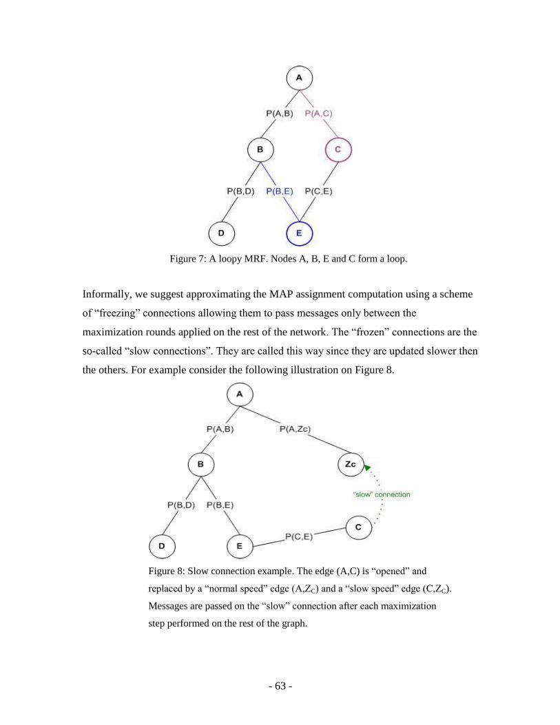
- 63 -
Figure 7: A loopy MRF. Nodes A, B, E and C form a loop.
Informally, we suggest approximating the MAP assignment computation using a scheme
of “freezing” connections allowing them to pass messages only between the
maximization rounds applied on the rest of the network. The “frozen” connections are the
so-called “slow connections”. They are called this way since they are updated slower then
the others. For example consider the following illustration on Figure 8.
Figure 8: Slow connection example. The edge (A,C) is “opened” and
replaced by a “normal speed” edge (A,ZC) and a “slow speed” edge (C,ZC).
Messages are passed on the “slow” connection after each maximization
step performed on the rest of the graph.

- 64 -
In this example, the slow connection is between the node A and the node C. The essence
of our approach, which will be described later in full detail, is as follows. During each
maximization round, A assumes some a fixed value of C (which was achieved in the node
C in the previous round). The assumption which is made by A is depicted on Figure 8,
where the node ZC is a so-called “evidence” node or observed node, value of which is
fixed during each maximization steps. Clearly, the network depicted in Figure 8 is a tree.
Hence, standard algorithms, such as GDL can be applied to calculate the MAP
assignment on this network. Between the maximization steps, the MAP value in node C
is transmitted to the evidence node ZC via the “slow” connection between them. This
value serves as the fixed value of the evidence node ZC for the next GDL maximization
round.
Removing loops by variable replication
Let us now formally introduce our approach of removing loops from the graph by
replicating some of the variables. At each step we choose a variable ix that is counted in
the weight of at least one of the current MST edges and which sub-graph induced by all
the nodes jS containing it ( ji Sx ) and edges of the current MST has two or more
connected components. We then choose a leaf jS belonging to the smallest of these
connected components (all the connected components are sub-trees of the MST and
hence must have leaves) and replace ix in jS by a variable ijz . Note that in each step
nSj
j decreases as n is increased (we add a new variable and ix remains in some
other node that was connected to jS in the current MST) and j
jS stays unchanged.
Moreover, the weight of all the edges between jS and its current neighbors in which ix
participated is decreased by one (edges whose weight becomes zero are removed).
If the new MST for the updated graph remains with the same weight, then the difference
between the weight of the current MST and nSj
j (where n is the current number of
variables and }{ jS are the current nodes of the “local domain graph”) decreases by one.

- 65 -
If the weight of the new MST decreases, then it is by no more then 1, as jS was a leaf of
the connected component and hence there was only one edge in the original MST which
was affected by the removal of ix from jS . Moreover, if the connected component was
the node jS alone then the weight of the new MST clearly remains the same as the
weight of the original one. Finally we note that every step reduces the size of at least one
connected component, hence arriving at points in which there are single-node connected
components is imminent. Hence, this process is guaranteed to converge to a point in
which the weight of the current MST will be equal to nSj
j for the current value of n
and the sets jS .
Assume the above process converges after m step and let ),,(11 mm jiji zzz denote the
vector of the variables added in the process. Let us denote by x~ - vector of all variables
from the set },,{1 mii xx and by y – vector of the all variables from the set
},,{\},,{11 miin xxxx . Then the “local domain graph” which has resulted after the
final step of the process represents a decomposition of a function ),~,( zxyg (with the
same local kernels as )(xf decomposition, but with updated domains of the local kernels
– some of the variables are replaced by z variables) which is loop-free, i.e. has a JT (as
this was the termination condition of the process). Moreover the MAP problem for the
)(xf can be updated to the new context as a constrained MAP (CMAP) problem :
),~,(maxargˆ~,~,
zxygxxzxy
, where the (consistency) constraint xz ~ means that
kkk iji xzmk :1 (note that x~ and y together compose the original x vector).
The choice of x~ and z in the above (a cut-set of the loopy network) is not unique in
general, some choices could be better then the others as we will see in the following
sections, where we discuss assumptions under which the CMAP problem can be solved
or approximated, together with approaches that make use of these assumptions. To
conclude this point, Figure 9 illustrates two possible z choices for removing loops from
an exemplar loopy MRF model. Each choice is depicted by coloring the local kernel
variables that are replaced with z variables.

- 66 -
Figure 9: Breaking Loops via creating “slow connections”. (a) A network containing a
loop. (b) One of the connections is „frozen‟ during a part of the computation; during
this computation the graph is effectively opened. (c) Another choice of “slow
connection”.
Finally we introduce a few notations that will make the discussion in the following
section more readable:

- 67 -
Instead of writing ),~,( zxyg we‟ll write ),,( zxyg where we‟ll assume (w.l.o.g.) that
x and z are of the same size (and ordered accordingly). All our results and approaches
can be extended in straightforward fashion from this case to the more general case
described above (in which z is potentially larger then x and several z variables can
correspond to the same x variable). Under this notation, the CMAP problem is a
problem of finding ),,(maxarg)ˆ,ˆ(,,
zxygxyxzxy
, that is argmax under the constraint
z=x. We will also refer to the constrained maximization as a problem of finding
“legal” optimums of ),,( zxyg , maximal points of the form ),,( xxy .
For any fixed z we denote: ),,(maxarg),(,
zxygxyxy
zz .
We denote the original function (the one over which we are interested in obtaining the
MAP assignment) by ),,( xxyg . In all the following discussions we‟ll assume that
),,( xxyg is loopy, while ),,( zxyg is loop free. In fact, the original function that we
have started with was ),( xyg , out of which we construct a loop free ),,( zxyg by
replacing some of the variables from x by variables from z. For example, x2 can occur
in more then one place, but we may replace it by z2 just in one of those places. The
function ),,( zxyg is strictly speaking different from ),( xyg , but ),(),,( yxgxxyg
for any x and y.
We assume that ),,( zxyg is discrete and bounded.
6.2. Approaches for obtaining a local optimum
In this section we describe several approaches for approximating the CMAP via iterative
processes, which converge to so-called “local optimum” points of g, of the form ),,( xxy .
Here “local optimum” means that some local changes (changes in specific subsets of the
whole set of variables) of the optimum point are guaranteed to decrease g.
For example, the function variables in the scheme, which is described in subsequent
section, are divided into two subsets. In each round of this iterative scheme, one of the
subsets is assumed fixed (i.e. being evidence variables) and in the next round the situation
is reversed. The value achieved in the previous round for each of the subsets serves as the

- 68 -
fixed value for the next round. The local optimum for this scheme is achieved with
respect to each of these subsets.
6.2.1. Iterative fixing
An approach that can be used to approximate CMAP is the “iterative fixing” approach.
This approach assumes that selection of z is “symmetric”, i.e. both the decompositions of
),,( 00 xxyg and ),,( 0 xxyg are loop free for any fixed 0x and 0y . In order to better
understand the symmetry assumption, you are referred to Figure 7, where we may
consider (C) to be the vector of x variables and (A,B,D,E) being the vector of y variables.
Then the above symmetry assumption clearly holds (fixing each of the vectors we arrive
to a loop free decomposition).
Given such a selection of z and the corresponding function ),,( zxyg we may
approximate ),,(maxarg)ˆ,ˆ(,,
zxygxyxzxy
by initializing 0zz and iterating the following
steps:
Fix kzz and calculate ),,(maxarg kky
k zzygy , as ),,( kk zzyg has a loop free
decomposition, this can be achieved using GDL for instance.
Fix kyy and calculate ),,(maxarg1 zzygz kz
k . The latter maximization is also
over a loop-free decomposition due to our assumptions on ),,( zxyg (the
“symmetric” assumption).
This iterative process terminates when kk yy 1 or kk zz 1 . Each step of the process
described above increases g over the previous point, and therefore:
),,(),,(),,( 11111 kkkkkkkkk zzygzzygzzyg
and since ),,( zxyg is bounded, the process is guaranteed to terminate. The termination
point of the process fits our “local optimum” description above as at point of termination
),,( lll zzy we have:
),,(),,( and ),,(),,(:, zzygzzygzzygzzygzy lllllllll
hence the only way to improve (i.e. increase g) from ),,( lll zzy is via changing both y
and z.

- 69 -
The above method was successfully used in [14] to calculate MAP (used for training their
model with “hard” EM) over a biological probabilistic model. The model in [14] was not
discrete, but the general steps of the algorithm were the same. As reported in [14] this
approach has produced very good results in their application.
Note that this approach is different from our proposed “slow connections” approach, as in
the slow connections approach the nodes with slow connections to other nodes are not
fixed and participate in maximization steps. In “slow connections” approach, nodes are
fixed only partially, that is they are assumed having some fixed value only be other nodes
connected to them via slow connections.
6.2.2. Local optimum assumption
From this section on, we‟ll discuss our novel techniques for MAP approximation. This
techniques form what we previously informally called the “slow connections” approach.
We derive several iterative processes using the following general approach as informally
introduced above: opening the loopy graph by duplicating some of the variables, and
iterating GDL and variable update. These processes are guaranteed to converge under
some assumptions about the original function. We will now describe the assumptions and
the processes.
The most basic of our approaches uses the following assumption to approximate CMAP
and obtain a “local optimum” for ),,( zxyg :
Assumption (A2) – weak z-minor:
),,(),,(),,(),,(: ZxygZZygZxygxxygy ZZZZZZZ
where ),,(maxarg),(,
Zxygxyxy
ZZ and inequality is strict unless ZxZ .
This assumption has the following meaning. For a fixed z=Z, we can maximize g, and the
maximum is obtained at ),,( Zxy ZZ. This is not a „legal‟ point, since by definition a legal
point has the form ),,( xxy . We can „legalize‟ the point in two different ways: either by
changing Z or by changing Zx . The assumption essentially says that z is a „less effective‟
variable: changing it from Z to Zx in points ),,( Zxy ZZ has a smaller effect than
changing x from Zx to Z and changing y.

- 70 -
Under the above assumption, a simple iterative process is guaranteed to converge to a
“local optimum” approximation of CMAP over ),,( zxyg . The maximize-and-legalize
process (denoted by P1) initializes by setting 0Zz (for instance we could first find the
global maximum ),,( 000 ZXY of loop free ),,( zxyg and take 0Z from there) and iterating
the following steps:
Maximization: Fix kZz and calculate ),,(maxarg),(,
kxy
ZZ Zxygxykk . As
),,( zxyg is loop free the latter maximization can be done using GDL.
Point legalization: Set kZk xZ 1 .
The iterative process terminates when kZ Zxk .
Claim 2: Assuming A2, the above iterative process converges to a point )~,~,~( xxy which
is a “local optimum” of ),,( zyxg in a sense that for any y and any kZ passed during the
process: )~,~,~(),,( xxygZZyg kk .
Proof: By induction. The induction hypothesis is:
),,(),,(:, 11 mmZkk ZZygZZygymkm
Initialization step: for m=0 the hypothesis trivially follows from the fact that
),,(maxarg),( 0,
00Zxygxy
xyZZ and thus ),,(),,(: 000 00
ZxygZZygy ZZ . Moreover
due to the A2 assumption:
),,(),,(),,(),,(: 0000 0000000ZxygZZygZxygxxygy ZZZZZZZ
and hence:
:y ),,(),,(),,( 000 00000ZxygxxygZZyg ZZZZZ or
),,(),,(),,(00000 000 ZZZZZ xxygZxygZZyg
Now recall that 01 ZxZ and thus the induction hypothesis results. Moreover, note that
inequality in the hypothesis is strict unless 00ZxZ .
Inductive step: Assume that inductive hypothesis stands for m-1 and let's show it for m.
By the hypothesis we get that:
),,(),,(:,11 mmZkk ZZygZZygymk
m

- 71 -
As ),,(maxarg),(,
mxy
ZZ Zxygxymm
, get that ),,(),,(: mZZmm ZxygZZygymm
and in
particular ),,(),,(:1 mZZmmZ ZxygZZygy
mmm
. Moreover due to A2:
),,(),,(),,(),,(: mZZmmmZZZZZ ZxygZZygZxygxxygymmmmmmm
and hence:
:y ),,(),,(),,( mZZZZZmm ZxygxxygZZygmmmmm
or
),,(),,(),,(mmmmm ZZZmZZmm xxygZxygZZyg
Finally, as mZm xZ 1 we get ),,(),,(:, 11 mmZkk ZZygZZygymk
m▄
Note that unless mZ Zxm the inequality above is strict, i.e. in this case:
),,(),,(:, 11 mmZkk ZZygZZygymkm
Conclusion: Since, as we have shown by induction, the sequence )},,({ mmZ ZZygm
is
strictly increasing, the process must converge (as g is assumed to be bounded). As
)~,~,~( xxy is the final point of the process, then there is some l for which
)~,~,~(),,( xxyZZy llZ l and hence, the claim follows immediately▄
6.3. Assumption for obtaining a global optimum
In this section we present another assumption on ),,( zxyg which is stronger then A2, but
at the same time guarantees that the process P1 described in the previous section
converges to the global maximum of ),,( xxyg (i.e. to the correct solution of the CMAP)
in a single step.
Assumption (A1) – strong z-minor:
),,(),,(),,(),,(:),(),(, ZxygZxygZxygzxygxyxyZz ZZZZZZZZ
where ),,(maxarg),(,
Zxygxyxy
ZZ .
Roughly speaking, A1 demands that, starting from a maximal point of the form
),,( Zxy ZZ, for any fixed Z and arbitrary z, changing Z to z has smaller effect on value of
g then changing the pair ),( ZZ xy to any other value ),( xy around the point ),,( Zxy ZZ .
Obviously A1 would not be true for a continuous function, but for a discrete function this
means that the z variable is "lateral", i.e. secondary, near the ),,( Zxy ZZ points Z .

- 72 -
Claim 1: Assuming A1, the maximize-and-legalize (P1) process will converge in a single
step to a global maximum of ),,( xxyg , i.e. the correct solution to the CMAP problem.
Proof: Denote by )ˆ,ˆ,ˆ( ZZy a global maximum of ),,( xxyg . We start the process P1 by
selecting an arbitrary Z value. We first maximize over y and x, to obtain ),,( Zxy ZZ, then
legalize to obtain ),,( ZZZ xxy . We will show that this process leads us to the global
maximum )ˆ,ˆ,ˆ( ZZy .
We first show that it must hold that Z
xZ ˆˆ . Assume for the sake of contradiction, that
ZxZ ˆ
ˆ . By A1:
)ˆ,,()ˆ,ˆ,ˆ()ˆ,,(),,( ˆˆˆˆˆˆˆ ZxygZZygZxygxxygZZZZZZZ
We also know that )ˆ,,()ˆ,ˆ,ˆ( ˆˆ ZxygZZygZZ
, from the definition of Z
y ˆ and Z
x ˆ . We
conclude that ),,( ˆˆˆ ZZZxxyg is strictly closer to )ˆ,,( ˆˆ Zxyg
ZZ than )ˆ,ˆ,ˆ( ZZyg is, and
therefore, ),,()ˆ,ˆ,ˆ( ˆˆˆ ZZZxxygZZyg in contradiction to )ˆ,ˆ,ˆ( ZZyg being a global
maximum of ),,( xxyg .
Figure 10: z-change vs. x,y-change. By A1 z-change from a
maximal point is always smaller then x,y-change.
Hence as Z
xZ ˆˆ and the global maximum point )ˆ,ˆ,ˆ( ZZy is a fixed point of P1. Since
),,()ˆ,,()ˆ,ˆ,ˆ( ˆˆˆˆˆ ZZZZZxxygZxygZZyg , and since )ˆ,ˆ,ˆ( ZZy is a global maximum of
),,( xxyg , then so is ),,( ˆˆˆ ZZZxxy .
Now let us choose some ZZ ˆ as the starting point of the process P1. Following the first
step of P1 we reach the point ),,( ZZZ xxy . We will show that this is in fact the global
- 73 -
maximum )ˆ,ˆ,ˆ( ZZy . Assume, for the sake of contradiction, that ),(),( ˆˆ ZZZZxyxy .
Consider the points ),,( ˆˆ ZxyZZ
and )ˆ,,( Zxy ZZ , by A1 applied to Zz ˆ and Zz :
(1) ),,(),,(),,()ˆ,,( ˆˆ ZxygZxygZxygZxyg ZZZZZZZZ
(2) )ˆ,,()ˆ,,()ˆ,,(),,( ˆˆˆˆˆˆ ZxygZxygZxygZxygZZZZZZZZ
From (1) we get that ),,()ˆ,,( ˆˆ ZxygZxygZZZZ . This is because
),,(),,( ˆˆ ZxygZxyg ZZZZ (from the definition of
ZZ xy , and from (1)) and
)ˆ,,( Zxyg ZZ is strictly closer to ),,( Zxyg ZZ than ),,( ˆˆ Zxyg
ZZ is. Similarly from (2) we
get that ),,()ˆ,,( ˆˆ ZxygZxygZZZZ , which is a contradiction. Hence
),(),( ˆˆ ZZZZxyxy . Therefore, P1 starting from arbitrary Zz converges in a single
step to the point ),,( ˆˆˆ ZZZxxy which is the global maximum of ),,( xxyg ▄
Remark: our proof also shows that the global maximum of a function which admits A1 is
unique.
6.4. Coping with general networks – from theory to practice
Assumptions and processes discussed in the previous section provide a useful tool for
MAP inference in certain types of loopy networks. However, two major problems can be
pointed out when applying them to the class of general loopy networks:
1. In general, assumptions strong z-minor (A1) or weak z-minor (A2) may simply not
hold. That is, not every function has a representation that has an appropriate selection
of z variables, so that A1 or A2 will be satisfied.
2. Even if for the given function representation, an appropriate selection of z variables
exists, finding it can be computationally intractable. That is, when the function‟s
support includes a large number of variables, selecting z variables and verifying A1
or A2 for a given selection can be exponentially hard. This is due to the fact that we
potentially have to consider all combinations of z and x, y variables.
In the following sections we will develop methods for addressing these issues, which can
be used for the practical application of A1/A2 based techniques. In addition, we will

- 74 -
derive an upper bound on the decrease in compotation complexity that can be achieved
by using our techniques, compared with the standard triangulation.
6.4.1. Partial iterative approximation
The first issue that we will address is the problem of assumptions A1 / A2 not holding for
a specific selection of z variables. Suppose we have a function whose decomposition
(here we assume that the function has a summation decomposition) can be expressed as
the sum of two parts: ),,(),( xxygxyf where x and y are vectors of variables.
Moreover, assume further that the decomposition of the ),( xyf part is loop free (i.e. has
a JT), while the decomposition of ),,( xxyg is loopy. However, if we replace the second
(vector) x by z we‟ll arrive at ),,( zxyg which is loop free (i.e. ),,( xxyg admits the z
selection as previously discussed). As an example, consider a function
),,(),,,( 3212121 xxxgxxyyf where ),(),(),,,( 2221112121 xyfxyfxxyyf and
),(),(),(),,( 133322211321 xxgxxgxxgxxxg , clearly ),,( 321 xxxg is loopy, while
),,,( 2121 xxyyf is loop-free. The problem we examine is that for the full function
),,(),( zxygxyf assumptions A1 / A2 do not hold.
Now assume there exists some small constant 1a s.t. assumption A1 holds for the
function ),,()],,()1(),([ 11 zxygaxxygaxyf . The last assumption is much less
demanding than assuming A1 for the original function ( ),,(),( zxygxyf ). This is
because the maximal function change caused by z is now controlled by 1a (multiplied by
it), and under relatively broad assumptions we can easily show that such 1a exists. A
sufficient assumption it that there is no zero differences for x, y changes, that is for any z
and any different pairs x1, y1 and x2, y2:
),,(),(),,(),( 22221111 zxygxyfzxygxyf
Recall that the maximize-and-legalize process (P1) under the A1 assumption converges to
the global maximum in a single step. The P1 process had two steps. First, fixing z to
some value and second maximizing over y, x. In the discussion above, this maximization
over y, x was performed by using GDL, since it was performed over a loop free

- 75 -
decomposition. In the current derivation we do not get immediately a loop-free function,
and we will deal with it in several steps.
The proof of P1 convergence implies that we can apply P1 by fixing 1Zz and
maximizing ),,()],,()1(),([ 111 Zxygaxxygaxyf for finding the maximizing
assignments x, y. If we can find this maximum, then after the maximization we simply
assign xz ˆ (where xy ˆ,ˆ is the maximizing y, x assignment) and terminate with a
maximal solution )ˆ,ˆ,ˆ( xxy .
To perform the maximization stage, we still need to maximize:
),,()1()],,(),([ 111 xxygaZxygaxyf
which is still not loop free. However, the first part (i.e. )],,(),([ 11 Zxygaxyf ) has a
loop free decomposition. As for the remaining part, ),,()1( 1 xxyga , we can proceed by
applying the same logic over again. We summarize the proposed iterative procedure by
describing step k of the iterative process:
1. At the beginning of step k the function that needs to be maximized is of the form:
),,()1(]),,(),([1
1
1
1
xxygaZxygaxyfk
i
i
k
i
ii
.
2. Find ka so the function:
),,(),,()1(]),,(),([1
1
1
zxygaxxygaZxygaxyf k
k
i
i
k
i
ii
satisfies A1.
3. Fix kZz and proceed to the next step (step k+1) in which we maximize the
function: ),,()1(]),,(),([11
xxygaZxygaxyfk
i
i
k
i
ii
.
The above process terminates when either one of the two conditions is fulfilled:
1. 11
k
i
ia , in this case we have to maximize ]),,(),([1
k
i
ii Zxygaxyf which is
loop free, and hence this can be done by GDL. The x, y pair which results from the
maximization is the correct solution to the original MAP problem, as follows
immediately from Claim 1 applied iteratively.

- 76 -
2. We also terminate in case we cannot find an appropriate ka in some step. In this case
we only arrive at solution to the MAP problem for the function: ),,(),( xxygcxyf
where
1
1
k
i
iac . This can be thought of as an approximation for the original MAP
solution that lies between completely ignoring the loopy terms and computing the
maximal assignment for the original function.
The heuristic choices that can be made in the above process are the selections of the kZ
constants which affect the subsequent steps of the process. Of course, the above approach
still suffers from the second problem of the A1 / A2 approaches, namely verifying that
A1 holds for a specific intermediate function (which is required for the ka selection) can
still be computationally expensive.
The final point that we can note about the process described in this section, is that it can
also be applied using A2 assumption instead of A1. In this case the maximization steps
will be a sequence of iterations, one for each successive fixed value of z. Moreover, each
iteration will apply recursively the successive “constant choosing” step of the modified
(for use of A2) algorithm. That is, as assuming A2, the P1 process does not converge in a
single step; we will need several iterative P1 steps for the maximization step (step 3) of
each intermediate function which arise in the partial iterative approximation process.
Each P1 step will recursively invoke the partial iterative approximation process for all
successive intermediate functions.
Example
As an example of an application of the above algorithm, consider the following simple
scenario. Assume we want to maximize a function ),,( 321 xxxg such that:
),(),(),(),,( 133322211321 xxfxxfxxfxxxg
Moreover, assume that functions (local kernels) 1f ,
2f and 3f are such that the strong z-
minor (A1) assumption does not apply in this case. However, assume that the local
kernels are such that we can apply the partial iterative approximation algorithm. Assume
that there exists 1a , such that:

- 77 -
),(),()1(),(),(),,,( 1331133121132213211 zxfaxxfaxxfxxfzxxxg
satisfies A1 around 11 Zz . Also assume that:
),()1(),(),(),(),,,( 2331133121132223212 zxfaZxfaxxfxxfzxxxg
satisfies A1 around 2Zz . Note that ),,,( 23212 Zxxxg is loop free and the procedure we
used to transform g into 2g is exactly 2-step partial iterative approximation algorithm.
If the A1 assumptions made in our example are satisfied, then the partial iterative
approximation algorithm applied to this example will terminate after a single
maximization step, as the resulting assignment to 321 ,, xxx will be the maximal
assignment to the original function due to claim 1 in section 6.3. Also note that 21 ZZ ,
as otherwise the original function would satisfy A1 if 3x is replaced by z in 3f .
However, if we replace one or both the A1 assumptions made in our example with A2
assumption, then the run of the partial iterative approximation algorithm will not
terminate in a single step. Instead it will run several maximize-and-legalize (P1) iterations
over 2g starting in
22 Zz until P1 converges, then it will legalize 1z (which started
from 1Z ) to a new fixed value and will run the maximize-and-legalize (again with respect
to 2z ) on the new function and so on. Both A1 and A2 variants of the partial iterative
approximation algorithm are illustrated in Figure 11.
Figure 11: Partial Iterative Approximation algorithm illustration. The nodes 1z and
2z start from the values 1Z and
2Z respectively. Under twice the A1 assumption
the process terminates in a single step and slow connections are not needed. In case
we assume only A2, we run maximize-and-legalize on 2z only, with
1z fixed, then

- 78 -
legalize 1z over the slow connection, then run maximize-and-legalize again, and so
on until convergence. The slow connections used in the process are of different
update “speeds”. The red slow connection is considerably slower then the green
one.
6.4.2. The hybrid approach
This section addresses the second problem arising in our approach for dealing with loopy
inference, which is the complexity of choosing the subset z of variables to keep fixed
during the maximization step. It is often hard and inefficient to select a set of appropriate
z variables to satisfy A1 / A2 in the ),,( zxyg construct. We approach this problem by
using the fact that, as noted briefly in the previous section, P1 can be used regardless of
whether the function in the maximization step is loop free or not. Indeed, assume we
express the function ),,( zxyg as ),,(),,(),( 21 zxygxxygxyf and assume that A1
holds for this function ),,(2 zxyg , while 1g is still loopy. If we have some way of
maximizing this function with z fixed, we can still use the maximize-and-legalize
approach: maximize the function with z fixed, then legalize it by setting xz ˆ where x is
the maximizing x assignment.
Using this fact, a plausible approach (in the efficiency sense) for solving MAP over a
given )(xf (loopy) decomposition, can be obtained by an iterative selection of variables
into the z vector. Variables that are being selected into z are variables that participate in
the loopy part of )(xf decomposition, i.e. each candidate variable should participate in
at least one loop. The resulting scheme has the following form:
1. First construct the local domain graph for )(xf decomposition.
2. At each step select at least one variable of one (or several) of the local domain nodes
of the current graph, so that the variable, taken as the z variable, satisfies A1. In other
words, if we denote the selected variable by x then ),,( zxyg function, which results
from )(xf if we replace x by z in the selected local domain(s) while denoting by y
the set of the remaining variables, satisfies A1 for z. We discuss below useful
heuristics for selecting these variables.
3. Fix Zz for some constant Z. By Claim 1 we know that:

- 79 -
),,(maxarg),,(maxarg,,
xxygZxygxyxy
4. Advance to the next step (either terminate if termination condition is satisfied or
return to step 1) by updating the local domain graph to represent the new ),,( Zxyg
decomposition into the sum (or product) of the updated set of local kernels. After
fixing the z variable in the selected local domain(s), the local kernel for that local
domain is updated accordingly to be a function of a larger set of variables (including
the new z variable).
5. Terminate when the local domain graph has a JT (i.e. represents a loop free
decomposition), or when no new z variable (or set of variables) can be selected.
As an example of the above method, consider the experiments run by us to test the “slow
connections” approaches. The setting of our experiments together with the detailed
description of applied algorithms is given in section 7, while the empirical results are
given in section 8.2.
Note that we could replace satisfying condition A1 in the above discussion by satisfying
A2. We can do so by making the maximization steps iterative. That is, each maximization
step - step 3, which operates on some iz selected in step 1 of the current iteration of the
scheme, would be consisted of several P1 iterations. Each P1 iteration will perform
maximization by recursively applying the following “z selection” steps (recursively
invoking step 1 on the updated local domain graph) and legalization by assigning new
value to the iz variable.
A more efficient version of working under A2 would be to iterate on the whole set of z
variables selected by all the steps, changing its value in each subsequent P1 iteration to
the corresponding x values. That is, instead of recursively applying P1 for each additional
variable selected into z, select the whole z vector and only then apply P1 for the whole z.
The latter version is not equivalent to the former one in the general case as selection of
subsequent z variables depends on the constants selected in the previous steps. However,
it can be used as a more efficient heuristics.
As an example of the above scheme augmented with A2, consider the “slow connections”
experiments which results are given in section 8.2. The “different slow speed” approach
uses recursive application of P1, selecting variables into z one by one and applying itself

- 80 -
recursively for each successive fixed value (resulting from legalization step of P1) of
each selected variable. The “same slow speed” approach selects the whole set of z
variables apriori and only then applies the P1 algorithm.
Although it can be beneficial in some cases, the above procedure has two limitations:
1. Selecting even a single or a small set of variables which satisfy A1 / A2 can be
problematic in some cases. This is because verifying A1 for instance, involves
estimating two values. The first is ),,(),,(max Zxygzxyg ZZZZz
, which usually
can be easily estimated for a single variable z which is selected in only a single local
kernel. The second is ),,(),,(max,
ZxygZxyg ZZyx
, which can be exponentially hard
in the general case. However, a useful heuristics might be selecting the z variable at
each step as being the one with minimum value of:
),,(),,(max,
ZxygzxygM ZZZZZz
z
The reasoning behind this heuristic is that if we restrict ourselves to a single z
variable selection, then selecting a z variable such that zM is not minimal means that
there is a non-z variable (the one resulting in minimum zM if selected into z) with a
smaller change then z, which potentially contradicts A1 / A2. Moreover, the ease of
selection of subsequent z variables can be manipulated by appropriate selection of the
Z constants in each step.
2. The procedure might terminate before all the “loops” are eliminated from the local
domain graph, that is, before the graph has a JT to which the GDL algorithm can be
applied. To address this issue, we combine the method proposed above with the
standard JT technique for coping with loops, which is the method of triangulation. As
discussed earlier in this work, using triangulation, a JT can be constructed for any
loopy network. In our case, triangulation can be applied, after the z selection process
can no longer proceed, on the “moral graph” which results from the decomposition of
the function of the final step of the process. From the triangulated moral graph
maximal cliques are extracted to form the nodes of the JT (as described in the section
5.1, discussing triangulation). This combination of z variables selection together with
the complementary triangulation, applied when the z selection can no longer proceed,

- 81 -
forms what we call below the “Hybrid Approach”. The advantage of this method over
the standard triangulation is in the potential reduction of the treewidth of the moral
graph. Note that the complexity of GDL applied to the triangulated network (i.e. on
the JT resulting after triangulation) is exponential in treewidth, hence fixing the
“lateral connections” potentially results in exponential decrease in the final GDL
computation complexity.
In the following section we will present an upper bound to the decrease in GDL
complexity that can be achieved by our techniques, while operating over a complete
“moral graph” with each edge represented by a local kernel.
6.5. Clique Carving
Assume having a function )(xf where ),,( 1 nxxx is its vector of variables. Assume
)(xf decomposes into a sum (not necessarily) of local kernels, of two variables each, so
the resulting “moral graph” is complete. I.e. )(xf has the following decomposition:
ji
jiij xxfxf ),()(
The treewidth (the size of the largest clique after triangulation) of the resulting moral
graph is n and GDL complexity for MAP for instance is clearly exponential in n. Now
assume we are using our hybrid approach on this problem:
Each time a variable ix from local kernel ),( jiij xxf is chosen and fixed, exactly one
edge from the moral graph is removed.
Suppose we‟ve succeeded in removing only one edge from the moral graph. The
resulting graph has exactly two maximal cliques (the first containing one of the
removed edge end nodes and the second containing the other). Each clique is of size
n-1 (thus the treewidth of the resulting graph is n-1) and most importantly, the graph
is triangulated (obviously, as any cycle of size more then three must contain at least
one node not adjacent to the removed edge and hence being connected to all the other
nodes on the cycle and thus the cycle has cords).
However if we remove exactly two edges, the treewidth of the resulting graph will
remain n-1, as triangulating it would yield back the graph with only one edge
removed (as the four nodes adjacent to the removed edges form a cordless cycle).

- 82 -
In general if we remove enough edges so the sub-graph induced by nodes adjacent on
the removed edges is a tree (or a forest) of m nodes, then the resulting moral graph
will be:
o Triangulated – as any cycle of length larger then three will involve at least one
node not from the tree. Moreover as this node is connected to all the nodes of the
graph (as none of its edges were removed). Thus in particular it will be connected
to all the nodes on the cycle giving it cords.
o With treewidth n-m+2. Obviously, as the largest cliques of the resulting moral
graph are consisted of all the non-tree nodes and exactly two tree nodes (taking
three or more tree nodes will not form a clique as there will be at least one edge
missing).
Thus the decrease in GDL complexity over the JT for the resulting moral graph is
exponential in m-2.
Moreover, the number of edges needed to “carve” a tree of size m (hence the name
“Clique Carving”) out of a complete graph is O(m2) (obviously). Hence the upper
bound to decrease in computation complexity that can be achieved by the hybrid
approach which succeeds in removing m edges (in the complete graph case) is
exponential in m .
Even more generally, we can rely on a well know graph theoretic result from [12]
which states that if every node of graph G1 is connected to every node of the graph G2
then treewidth of the resulting graph: 21 GG is given by:
})(,)(min{)( 122121 VGtreewidthVGtreewidthGGtreewidth
where V1 and V2 represent the vertex sets of G1 and G2 respectively. Thus if we
“carve” out a graph of treewidth k and with m nodes then the treewidth of the
resulting moral graph will be mnkmmnmnk },min{ , as mk . Thus
the upper bound on GDL complexity decrease that the hybrid approach can provide
us in this case is exponential in m-k.
We conclude this section by noting that in case of a complete moral graph, the worst case
that can be considered in sense of the hybrid approach is the one discussed above, i.e. the

- 83 -
case of local kernels with size two domains (obviously, as in this case hybrid approach
eliminates one edge for each z variable selection).
7. Applying “Slow Connections” approaches in practice
We performed a set of computational experiments to test the performance of the “slow
connections” MAP approximation schemes described above. These tests utilized a
graphical model that we call a “clique-tree” graph. In the clique-tree, there are several
cliques which are connected together in a form of a tree. The clique-tree results from a
tree by connecting every node to all of its siblings (children of its parent) in the original
tree. The function maximized over the clique tree was the sum of the logarithms of the
edge weights of the tree plus sum of logarithm of local weights of the nodes. That is, in a
clique tree G, the function to be maximized was:
)()(),(
)()),(log()(GVv
ii
GEvv
jiij
iji
vfvvwGf
where the arguments of the function (such as ji vv , ) were variables residing in the nodes
of G.
The experimental testing used the algorithm described in the “hybrid approach” section.
This computation can also be regarded in a more simplified manner as a message passing
algorithm, with some messages proceeding slower than others in terms of the message
passing speed. Moreover, let the junction graph, consisting of only the “faster” links, be a
tree (i.e. it has no loops). Then the algorithm can be viewed as iteratively running GDL
(i.e. standard bottom-up, top-down algorithm) on the “faster” links tree, then passing the
values obtained from the GDL over the slow links to serve as “initial messages” (for the
next GDL iteration) received over these links. These messages affect the values of the
GDL local kernels. In this general setting there are several factors that may vary to
produce different algorithms:
1. The selection of the subset of slow edges (as well as their directions) is a key factor
for the performance of the general algorithm above as a MAP estimator. In our
experiments, we compared several approaches for the slow edges selection. The
tested variants included “iterative A2 selection” and “random selection” (explained
further below).

- 84 -
In addition, the slow edges may be fixed (i.e. the same slow edges are used during the
entire progress of the algorithm), or they may be re-selected during runtime, and
thereby affect the message passing schedule. In our experiments, we tested both the
fixed and the varying slow edges schemes.
2. The slow edges “speed” may vary. The slow edges may be updated together or
updated by some specific schedule. If we allow the slow edges speed to vary, we may
further improve the results under A2 assumption, as we then can apply A2
recursively, fixing one edge at a time and iterating over it (recursively applying the
same fixing algorithm) as long as there is improvement. However, this approach is
potentially much less efficient in cases there are many loops, because every loop
appears in the recursion and then the run-time complexity is potentially exponential in
the number of loops. In our experiments we tested both the alternatives.
All the tested algorithms iterated three kinds of steps:
1. Edge removal step – at this step an edge or a set of edges were selected, together
with fixing their directions. By fixing direction of an edge ),( ji vv with edge weight
)),(log( jiij vvw we refer to selecting either iv or jv to be “fixed”, and be the sender
of the slow edge update after the GDL step. After one of the edge directions is fixed,
the weight of the fixed edge becomes part of the local weight of the node which was
not fixed (i.e. if iv was selected in the direction selection then jv ‟s local weight is
updated).

- 85 -
Figure 12: Edge removal step. G1 and G2 are connected components of the graph. The
functions )( ii vf and )( jj vf are local weights of iv and jv , while iZ is the fixed z
value selected for iv when edge ),( ji vv is removed. The “slow connection”, drawn
using green dots below, supplies jv with new values of iZ , which are the maximizing
values of iv from the previous maximization iteration.

- 86 -
2. Contraction step – after one or more edges are fixed, some nodes may become
connected to the rest of the graph by means of a single edge only. The algorithm
readily runs the GDL update step from these nodes and removes them from the graph.
The messages passed in the update steps, which are the standard GDL messages over
max-sum semi-ring, are incorporated in the local weights of the nodes receiving them,
as they are functions of the receiving node alone (this follows directly from the
definition of the GDL messages).
Figure 13: Edge contraction step. The functions )( ii vf and )( jj vf are local
weights of iv and jv , while )( jij vm is the standard GDL message defined as:
),(log)(max)( jiijiv
jij vvwvfvmi
.

- 87 -
3. Split step – after one or more edges are fixed some edges may become “splitting
edges” of the graph. A splitting edge is an edge removing which disconnects the
graph into two connected components. When splitting edges result, we view each of
the resulting (loopy) connected components as nodes of a “super” tree connected via
the splitting edges. We then run the standard GDL algorithm over the “super” tree
using our algorithm inside each connected component for the maximization steps of
the GDL.
Figure 14: Split step. G1 and G2 are connected components of the graph connected by a
single edge ),( ji vv . The maximizing assignment is computed using GDL on the “super”
JT below. The “super” JT has vertices G1, G2 and ji vv , , the latter has a local kernel
),(log)()( jiijjjii vvwvfvf . Maximum in G1 and G2 nodes is computed using the
“slow connections” algorithms.
Each edge removal step could lead to contraction or split step or alternatively to the
following edge removal step. Contraction step may lead to other contraction steps. In

- 88 -
general it is better to run all the possible contraction steps prior to the split steps in order
to keep the process simpler, as otherwise, single nodes may be unnecessarily regarded as
connected components – candidates for contraction which is less efficient.
8. Experimental results
The next sections present the experimental results we obtained for our two novel
approaches: the Max-MI training method, and the Slow Connections MAP
approximation. The results for Slow Connections algorithm also contain comparison
results with other MAP approximations, such as the commonly used Loopy Belief
Revision.
8.1. Max-MI classification model training
Problem setting
The problem we consider is object recognition. We construct and train feature based
models that are used to solve this problem. In order to use a feature based model, we need
a way to find a visual feature in an input image. The features that we use in our
experiments are image patches. For example, on Figure 15 features are parts of a face,
and on Figure 16, parts of a cow. Each feature is represented hierarchically in terms of
simpler sub-features. Each feature is searched in the image by normalized cross-
correlation, and it has two parameters: a threshold θ and a region of interest (ROI). A
feature Fi is detected (Fi = 1) if its correlation exceeds its threshold θi. It is searched in
the image within a limited window given by the ROI with respect to the position of its
parent node. We are given a set of features, and the problem we consider is the
construction of an optimal TAN structure, and the optimal setting of all the thresholds
and ROI values, such that the resulting model will have the maximum prediction power
for object recognition.
Our goal is to recognize a visual object on unseen images using the trained models. The
visual objects that we recognize in our experiments are part of the face and part of a cow,
and the models are trained over face image database and cow image database
respectively.

- 89 -
Experimental setting
The results of this part consist of experiments conducted on two models of different size.
The first was a “face parts” model consisting of 12 feature nodes, as depicted in Figure
15.
Figure 15: Original face parts model. Features are image patches which form a
hierarchy in which the larger patches appear at the top and the smaller patches appear
at the bottom. This model was constructed for face vs. non-face (binary class)
classification.
The second model was a cow parts model, consisting of 26 feature nodes as depicted in
Figure 16.
Figure 16: Original cow parts model. This model was constructed for cow vs. non-cow
(binary class) classification.
The trained parameters were feature thresholds and ROI. We have tested both the
thresholds + ROI training and thresholds only training. In the experiments which trained

- 90 -
thresholds alone, the ROI was set to some fixed, preset value. Note that although we have
used binary features (one threshold per feature) and a single ROI window per feature, we
could as well train several thresholds and ROI windows for each feature, using the same
learning approach.
Learning the ROI parameter poses a special problem for the MaxMI combined with TAN
restructure scheme. The problem comes from the nature of ROI parameter. The ROI is a
search window of a feature, which is specified with respect to the feature‟s parent
location. Thus it is problematic to apply the conventional TAN restructure algorithm
introduced by Friedman et al. in [2]. As even when ROI is fixed, one needs to assign Fi
parent Fj or Fj parent Fi in order to compute the edge weight MI(Fi,Fj;C), since the result
will be potentially different for each choice of edge direction.
In the context of the visual interpretation problem described above, the original feature
hierarchy is rather strict. That is, it usually makes no sense to reverse parent–to-
descendants relationships. Hence, a possible solution to ROI training problem in this
context is using “constrained TAN” restructure step instead of the conventional TAN
restructure step. This means that, instead of computing MST on a full graph, we would
compute a directed MST on a “layered” graph consisted of several fully connected layers.
Each layer would consist of features residing at the same depth in the current feature tree.
For each edge, the parent node would be the node with smaller layer number, where the
layer number of a node is its depth in the feature tree. The results of applying the
constrained TAN heuristic are summarized in the Tables 1 and 2 below. The schematic
representations of the models restructured using the constrained TAN heuristic are given
in Figures 17 and 18.
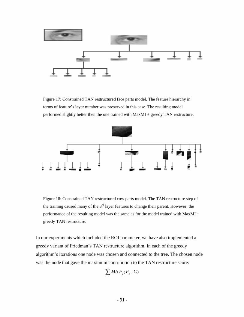
- 91 -
Figure 17: Constrained TAN restructured face parts model. The feature hierarchy in
terms of feature‟s layer number was preserved in this case. The resulting model
performed slightly better then the one trained with MaxMI + greedy TAN restructure.
Figure 18: Constrained TAN restructured cow parts model. The TAN restructure step of
the training caused many of the 3rd
layer features to change their parent. However, the
performance of the resulting model was the same as for the model trained with MaxMI +
greedy TAN restructure.
In our experiments which included the ROI parameter, we have also implemented a
greedy variant of Friedman‟s TAN restructure algorithm. In each of the greedy
algorithm‟s iterations one node was chosen and connected to the tree. The chosen node
was the node that gave the maximum contribution to the TAN restructure score:
)|;( CFFMI kj
- 92 -
That is if the set of tree nodes added before iteration i is denoted by iT then the node
chosen in iteration i was:
)|;(maxmaxarg\
CFFMIF kjTFTSF
mij
ik
where S stands for the set of all the nodes from which the tree is formed. The chosen
node mF was connected to the node of iT in which the maximum of the inner term was
obtained.
Increasing the TAN restructure score in turn increases the log-probability of the TAN
model, thus applying even the greedy variant of the algorithm is still reasonable. The
schematic representations of the greedily TAN restructured face and cow models are
given in Figures 19 and 20. The numerical results of greedy TAN heuristics application
are summarized in Tables 1 and 2.
Examining the different options for TAN learning, it can be seen from these results, that
on the cow image database, constrained TAN performed slightly better then the greedy
TAN heuristic in terms of the error rate.
However, it performed worse then the greedy TAN over the faces image database, again
in terms of the error rate. The reason is probably overfitting since the MI of the model
trained using constrained TAN is higher then of the greedy TAN (over the faces image
database), and so is the error rate over the training images. We conclude that the choice
of proper TAN restructure heuristic in cases where the original TAN restructure step
cannot be applied (for e.g. when we train ROI parameters), is implementation dependent.
More experiments with various image databases may also shed some light over the
governing dynamics of the best TAN heuristic choice in our context.

- 93 -
Figure 19: Greedy TAN restructured face parts model. The resulting model performs better then
the model with the original structure (both trained with MaxMI). However, the resulting tree
structure is not as intuitive as the structure obtained with constrained TAN restructure
algorithm.
Figure 20: Greedy TAN restructured cow parts model. The greedy restructure step has
“flattened” the model in a sense that most of the lowest level features became direct children of
the root node. Again, although the performance was improved relative to the original structure,
this tree construct is not intuitive.
Note also that in the experiments involving the threshold parameters only, the original
TAN restructure (MST over the )|;( CFFMI kj edge weights) was applied.
Although the alternative hybrid approach presented at the end of Section 4.4 looks more
promising then the MaxMI & TAN restructure iterations suggested at the beginning of
that section, our empirical experiments have shown otherwise. The results of the
alternative hybrid approach were less good then of the MaxMI & TAN restructure
iterations. One possible reason is data specific; it is possible that more tests with other
- 94 -
test / training data sets would show otherwise. We suggest that more empirical and
theoretical research of the alternative hybrid approach would shed more light on its
performance.
The numerical results are summarized in the tables below in Tables 1 and 2. The original
training refers to parameters obtained by another method (computed during feature
selection in [8]).
Results summary
It can be seen that several versions of the MaxMI and TAN learning significantly
outperformed the original training method used in [8] during the feature selection. The
original training method chose the feature parameters by maximizing the local Mutual
Information terms: );( CFMI i where C is the class variable and Fi is each feature taken
separately. Due to the specific choice of the faces image database, the difference between
MaxMI (without TAN restructure) training and the original training is insignificant on the
faces image database. However, it is highly significant (~36% improvement using
MaxMI) on the “more difficult” cow image database.
In addition, the MaxMI with constrained TAN and greedy TAN methods gave
significantly better error rates then the original training on both image databases.
Moreover, using TAN restructure steps improved the error rates of the MaxMI algorithm
alone. The performance improvement over the MaxMI training alone, introduced by
TAN restructure steps, was especially significant on faces image database (~45% with
greedy TAN restructure) and less significant on cow image database (~16% improvement
with constrained TAN restructure).

- 95 -
Face Parts Model
Test DB
Size
Training DB
Size
Class entropy on
training DB
MI model to class on
training DB
Error rate on
test DB
Error rate on
training DB
MaxMI Training 2257 767 0.792690834 0.758242464 135 25
Original Training 2257 767 0.792690834 0.722429352 136 35
MaxMI Training with
constrained TAN
restructure 2257 767 0.792690834 0.756855168 Miss=62, FA=36 Miss=15, FA=3
MaxMI Training with
greedy TAN restructure 2257 767 0.792690834 0.746516913 Miss=30, FA=44 Miss=16, FA=3
Alternative MaxMI Training
with TAN restructure 2257 767 0.792690834 0.74711484 Miss=33, FA=109 N / A
Threshold only training
(without restructure) 2257 767 0.792690834 0.738676981 Miss=84, FA=46 Miss=30, FA=5
Observed & Un-observed
model training constructed
from the all-observed model
and soft EM 2257 767 0.792690834 N / A 67 N / A
Table 1: Information based training results summary for the face parts model

- 96 -
Cow Parts Model
Test DB
Size
Training DB
Size
Class entropy on
training DB
MI model to class on
training DB
Error rate on
test DB
Error rate on
training DB
Original Training 2256 961 0.46535663 N / A Miss=84, FA=64 Miss=36, FA=16
MaxMI Training 2256 961 0.46535663 N / A Miss=53, FA=42 Miss=25, FA=17
MaxMI Training with
constrained TAN
restructure 2256 961 0.46535663 N / A Miss=32, FA=48 Miss=17, FA=12
MaxMI Training with
greedy TAN restructure 2256 961 0.46535663 N / A Miss=59, FA=30 Miss=23, FA=16
Observed & Un-observed
model training constructed
from the all-observed model
and trained using soft EM 2256 961 0.46535663 N / A 89 N /A
Table 2: Information based training results summary for the cow parts model
- 97 -
8.2. “Slow Connections” approximation
Problem Setting and implementation details
Our experiments were conducted over a special class of loopy networks, the so-called
“clique-tree” networks. The essence of a clique tree network structure is that is a super-
tree of cliques, each two “connected” cliques in the tree are connected via a single edge
between a node in one clique and a node in the other clique. The structure of a clique-tree
network is illustrated on Figure 21.
A structure similar to the clique tree network arises in many interesting applications. A
clustering technique, such as triangulation, can be applied to any loopy belief network to
produce a junction tree with enlarged local domains. The local kernels for the enlarged
domains are aggregates of several original local kernels, which domains were clustered
together to form the enlarged local domain.
We denote by T the “tree” of the clique-tree network, i.e. the tree which nodes are
actually cliques of the network. In fact, T is a junction tree of a clique-tree network, and
local domains of T are the network‟s cliques. Hence, in order to compute the MAP
assignment to the nodes of the network, we ran a GDL on T.
Maximization steps of the GDL, which are used to compute messages from some clique
Ci, needed to maximize the sum of all the weights of edges of nodes of Ci plus the single
node messages received from neighboring cliques. We used our slow connections
algorithm in order to perform this maximization. The messages received from
neighboring cliques (all of which are functions of a single node due to the structure of the
junction tree T) were incorporated into the local weights of the appropriate clique nodes
prior to the slow connections run. The slow connections run iterated (in this order) edge
removal, contraction and split steps, described in detail in section 7, until the approximate
maximum and maximum assignment were computed.
Different slow connection techniques differed in the split steps iterations. Each such
technique used a different paradigm for selecting the edges to remove and replace by a
slow connection.

- 98 -
Figure 21: Structure of the clique-tree network. The network is a tree of cliques, each two
neighboring cliques connected via a single edge. Each node iv of the resulting graph has a local
weight )( ii vf attached to it and weight of an edge ),( ji vv is denoted ),(log jiij vvw . Our goal
is to maximize i
ii
ji
jiij vfvvw )(),(log and find the maximizing assignment (argmax) to
all the nodes }{ iv . That is, solve the MAP problem on this loopy network.

- 99 -
Experimental Setting
Our experiments compared the performance of different types of our “slow” connections
algorithm with the standard Loopy Belief Revision (LBR) algorithm, which is a popular
approach for dealing with loopy graphical models. In our experiments we used two
stopping conditions for the LBR:
A node will not forward messages (updated with its local kernel) if the argmax (with
the node variables as arguments) over all messages received from its neighbors
including the last message, does not change. That is, the last message did not change
the node maximizing assignment, although it could change the maximum value
reached.
A node will stop forwarding messages after it has reached its maximal allowed quota
of forwarding messages. That is, each node will be allowed to forward at most k
messages, where k is a pre-determined parameter. In our experiments we used k=50
and k=10.
Our empirical experiments indicated this variant of LBR produces reasonable results in
many cases. However, it was outperformed by our proposed “slow connections”
approach.
We compared the following cases:
Weak z-minor (A2) with different "slow" speeds
The edge removal step of this algorithm greedily selected edges with minimal
“variation” (difference) from all the available edges and selected the “fixed”
directions which gave the minimal difference. As mentioned in section 6.4.2 selecting
edges that can be made slow, that is edges which weights satisfy one of the A1 or A2
assumptions relative to the rest of the graph, is problematic in general. The problem
lies in efficiency of verifying that A1 or A2 assumption indeed holds. Hence, we used
the following heuristic for selection of slow edges and their directions.
At each edge removal step the edge selected to be removed and replaced by a slow
edge was:
),(log),(logmaxminmaxminarg),(),(
jiijjiijvZvvv
ji vZwvvwvviij
ji

- 100 -
The reasoning behind this selection is that we want to find an edge with minimal
variability, i.e. with minimum effect when we fix one of its directions by turning one
of its nodes into a z-variable. We measure variability by maximizing over all the non-
fixed variable values the minimum over all possible fixed variable values of the
maximum the z-difference. The maximum z-difference is for a given fixed value Zi is
),(log),(logmax jiijjiijv
vZwvvwi
(here we consider vi as a candidate for becoming
z-variable of the edge ),( ji vv ).
The initial fixed value of the z-variable of the edge ),( ji vv made slow at edge
removal step was the one providing minimum over all values of vj maximum z-
difference:
),(log),(logmaxminminarg jiijjiijvvZ
i vZwvvwZij
i
At subsequent steps of the slow connections algorithm the fixed value was updated in
the legalization steps of the maximize-and-legalize (P1) algorithm.
If our heuristic succeeded in choosing slow edges, such that each of them satisfied A1
or A2 with respect to the network state at the time the choice was made (during each
edge removal step), then the applied slow connections algorithm is guaranteed to
converge to a local or a global optimum depending on which assumptions A1 or A2
are satisfied at each slow edge. We call the assumption that: all the selected edges
satisfy A1 or satisfy A2 with respect to the state of the network at the time they were
selected, “iterative A1” or “iterative A2” respectively.
By using different slow connection speeds we refer to applying A1 or A2 at each
edge, selected to be slow, separately. This means that we apply the maximize-and-
legalize (P1) algorithm on each slow edge by itself with respect to the state of the
network at the time this edge was selected, i.e. when the according edge removal step
was applied.
Using different slow connection speeds, we get a recursive algorithm which is
guaranteed to achieve the global optimum under “iterative A1” assumption and local
optima under “iterative A2” assumption. However, the convergence speed of this
algorithm is not guaranteed under A2 assumption and even tends to be exponential in

- 101 -
the number of loops. Under A1 it is linear in the size of the graph as each P1
application terminates in one step.
Weak z-minor (A2) with same "slow" speeds
This method is the same as above, only all the slow edges were updated over
simultaneously. That is, in this case the slow connections were selected once with
their fixed directions and initial fixed values and the slow connections algorithm that
was applied was the original maximize-and-legalize (P1) in which all the slow
connections fixed directions were the z-variables. This algorithm can be regarded as a
synchronous distributed algorithm operating under a global clock. At even clock ticks
(starting from the zero tick) the algorithm runs a GDL message passing algorithm on
all the fast (that is non-slow) edges of the network, that is runs the maximize step of
P1. At odd clock ticks the algorithm propagates the values obtained in the previous
(GDL) tick over the slow connections, in the fixed direction, i.e. from the z-node to
the other node, so that in successive (even) clock tick these values will be
incorporated as the new fixed Z values in the local kernels over which the GDL is
run.
Experimentally, this approach operated in liner time, that is the number of times
needed until the function being maximized (over the whole clique) stopped increasing
was relatively small.
Random Slow Connections
The slow connections and the fixing directions were selected at random and were
updated over simultaneously (i.e. were of the same speed).
The numerical results are summarized in the following tables. The rows represent
different kinds of test sets. In randomly generated test sets, the test sets differ in the
number of possible values for each node. Moreover, we tested over clique-trees generated
from face classification models with edge and local weights based on “natural”
distributions of the features in the models.
Following is the explanations of the terms used in the tables:
Model Size – the depth and the branching of the clique-tree. The depth is the number
of levels in the tree of cliques plus one. The branching is the size of each clique minus

- 102 -
one. For example, depth = 3 and branching = 5 clique tree, has six cliques, each of
size 6.
Node Count – is the number of nodes of the clique-tree, or the number of variables in
the maximized function.
Value Count – the number of values that each variable can take. For example if value
count is two then we maximize a function with binary variables, while if it is four
then every node has four possible values.
Sample Count – the number of clique-tree networks that were generated. The
average approximation rates were calculated over all these networks. The networks
were either randomly generated or constructed from “natural” examples such as
feature trees used in MaxMI experiments. All the corresponding rows of all of the
tables represent experiments performed on the same generated set of networks.
Average Approximation – the percent of the true maximum value obtained averaged
on all the sampled clique-tree networks. The percent is over the difference between
the true maximum value and the true minimum value. The true max. and min. values
were calculated using exhaustive search.
Average Mismatch – the average number of values in the approximate maximal
assignment which differ from the values of the true maximal assignment. The average
is calculated over all the generated samples.
Average Match % - the average percent of the values of the approximate maximal
assignment, which match the values of the true maximal assignment. The percent is
taken over the node count.
Models based on natural feature trees – the clique-tree networks generated from
observed & unobserved feature trees similar to ones used in MaxMI experiments. The
clique-trees were constructed from the unobserved nodes of the feature tree. The
clique-tree structure and edge weights of all the sample models was the same, the
only difference between the models was varying local weights which represented
evidence input. That is, for each test image of the feature tree, the local weight of the
node was set to the probability measure of the corresponding unobserved node being
1 or 0 given the value of its attached observed node calculated from the test image.

- 103 -
We compared the results obtained by the different methods using statistical test. We
compared by paired t-test the significance in performance differences between A2 (same
"slow" speed) and Belief Revision (50 messages) when applied to the depth 3, branching
5, 3-valued model. The difference in performance between slow connections technique
and Belief Revision was highly significant, 1010p , n=1000, two-tailed paired t-test. In
addition, the slow connections method was superior, 1010p , one-tailed paired t-test.
Moreover, t-test established with confidence > 0.9999 that the true interval for the
difference mean is 5.2% to 6.2% for the benefit of the slow connections scheme (the units
of the difference mean are percents of the difference of true maximum and true minimum
of the test models).
This result was confirmed by Wilcoxon’s “Signed Rank Test”, yielding 15010p
probability for the means of the corresponding performance data to be equal.
Summary
From the results obtained from the experiments we can see that slow connections based
algorithms significantly outperform both simple loopy MAP approximations, like
ignoring the loopy links and maximizing on the resulting tree, and more complex
algorithms like the popular Loopy Belief Revision (LBR).
Among all the slow connections algorithms, the more promising one is, to our opinion,
the weak z-minor based “same speed” slow connections algorithm. There are two reasons
that make it the preferred choice. One is that it is far more efficient then the different
speed variant that is likely to be exponential in the number of loops of the network. The
other reason that makes it interesting is that there are reasons to believe, that in the
human brain there are constructs of fast and slow links, where the fast links perform an
up-and-down computations and the slow links pass their messages between such
computations. This lies in complete parallel with what the “same speed” algorithm does,
hence an interesting research direction is trying to explain some of the brain functions
using this algorithm.

- 104 -
Model Size Node Count Value Count Sample Count A2 (different "slow" speed)
Average
Approximation
Average
Mismatch
Average Match
(%) Depth=3,
Branching=5 31 4 1000 98.26% 10-11 65.22%
Depth=3, Branching=5
31 3 1000 98.08% 7-8 74.51%
Depth=3, Branching=5
31 2 1000 98.55% 3-4 88.62%
Based on Natural feature trees, 4 cliques of size 7
25 2 ~2000 97.85% 3-4 86.14%
Model Size Node Count Value Count Sample Count A2 (same "slow" speed)
Average
Approximation
Average
Mismatch
Average Match
(%) Depth=3,
Branching=5 31 4 1000 94.11% 15-16 50.31%
Depth=3, Branching=5
31 3 1000 94.55% 11-12 63.70%
Depth=3, Branching=5
31 2 1000 97.16% 4-5 84.60%
Based on Natural feature trees, 4 cliques of size 7
25 2 ~2000 98.34% 1-2 93.62%

- 105 -
Model Size Node Count Value Count Sample Count Random Slow Connections
Average
Approximation
Average
Mismatch
Average Match
(%) Depth=3,
Branching=5 31 4 1000 82.70% 20-21 34.58%
Depth=3, Branching=5
31 3 1000 81.52% 16-17 45.48%
Depth=3, Branching=5
31 2 1000 79.37% 11-12 62.23%
Based on Natural feature trees, 4 cliques of size 7
25 2 ~2000 N/A N/A N/A
Model Size Node Count Value Count Sample Count Loopy Belief Revision (50 messages per node)
Average
Approximation
Average
Mismatch
Average Match
(%) Depth=3,
Branching=5 31 4 1000 N/A N/A N/A
Depth=3, Branching=5
31 3 1000 89.17% 13-14 55.31%
Depth=3, Branching=5
31 2 1000 88.73% 8-9 72.80%
Based on Natural feature trees, 4 cliques of size 7
25 2 ~2000 93.34% 3-4 87.73%

- 106 -
Model Size Node Count Value Count Sample Count Loopy Belief Revision (10 messages per node)
Average
Approximation
Average
Mismatch
Average Match
(%) Depth=3,
Branching=5 31 4 1000 87.65% 17-18 41.95%
Depth=3, Branching=5
31 3 1000 86.74% 14-15 54.02%
Depth=3, Branching=5
31 2 1000 85.78% 8-9 71.80%
Based on Natural feature trees, 4 cliques of size 7
25 2 ~2000 N/A N/A N/A
Model Size Node Count Value Count Sample Count Ignore Sibling Loopy Links
Average
Approximation
Average
Mismatch
Average Match
(%) Depth=3,
Branching=5 31 4 1000 74.04% 21-22 29.25%
Depth=3, Branching=5
31 3 1000 71.89% 19-20 38.56%
Depth=3, Branching=5
31 2 1000 69.38% 13-14 56.09%
Based on Natural feature trees, 4 cliques of size 7
25 2 ~2000 73.45% 9-10 63.88%

- 107 -
9. Summary and conclusions
In this section we summarize the novel results developed as part of this work. The results
presented in this thesis are divided into two topics. The first topic is information based
training, under which we have developed several novel graphical models training
algorithms based on what we call the MaxMI training framework. The second topic is
loopy MAP approximation, for which we have developed a family of the so-called slow
connections algorithms. Following is a list which covers all the main results developed in
the thesis in their presentation order.
MaxMI based training
We have developed a MaxMI training algorithm for training parameters of graphical
models for the purpose of classification. MaxMI is information maximizing training
algorithm, which is designed for training feature parameters of all-observed TAN
classification models. It can also be applied to general loopy belief networks, but it is
efficient only in cases that the model‟s graphical representation has low treewidth.
We have shown that under specific assumptions, the MaxMI algorithm maximizes the
mutual information between the model and the class. This means, that if the all-
observed model consists of a vector of features F and a class variable C, then the
parameters trained by the MaxMI algorithm maximize );( FCMI . The main
difference between the MaxMI algorithm and other information based training
techniques, such as maximizing mutual information for each feature separately, as in
[8], or maximizing the minimum pair-wise information increase (where ji FF , are
elements of F): );(),;( jji FCMIFFCMI , as in [24], is that MaxMI, if its
assumptions are satisfied, guarantees to find the feature parameters that maximize the
mutual information of the entire feature vector with the class (for a given model
structure).
Experiments performed to test the performance of the MaxMI algorithm, revealed
that is in fact superior to the previous information based approaches. To our opinion
this algorithm has a potential of becoming one of the state-of-the-art training
algorithms for loop-free graphical models.

- 108 -
We have presented extensions to the MaxMI training algorithm for the case in which
the classification model is constructed of both observed and unobserved (O&U)
nodes. These types of models are especially useful for solving visual interpretation
problems, since their unobserved nodes can be regarded as representing the
interpreted parts of the visual object. We have presented two extensions of the
MaxMI algorithm to this case.
The first was a straightforward augmentation of the MaxMI algorithm to support
unobserved nodes. However, it is inefficient if applied to special cases of O&U
models – the observed-in-leafs-only case. In this case, all the observed nodes of the
loop free O&U models are attached only to the leaf unobserved nodes and none of
them is attached to the inner unobserved tree nodes.
The second was applying the original MaxMI algorithm to the observed nodes of the
model alone, obtain the optimal parameters in this case, and train the original model
unobserved to unobserved and unobserved to (trained) observed with soft EM.
Learning feature parameters using EM alone is infeasible, as changing observed
feature parameters, changes the EM training data. A method of applying the soft EM
to TAN models was also developed in the background coverage part of this work.
The second technique of O&U model training was tested as part of our empirical
experiments and exhibited an improvement in the performance over the all-observed
model. This suggests that it has a potential of contributing to visual interpretation
research in the future.
We have developed two hybrid techniques involving both MaxMI and N. Friedman‟s
optimal TAN construction algorithm [2]. These techniques provide a method for not
only training optimal feature parameters, but also constructing optimal TAN model
structures.
The first hybrid technique involved iterative application of a MaxMI parameter
training step followed by a TAN restructure step. The MaxMI step searched for
optimal feature parameters for the given model structure, and the TAN restructure
step searched for optimal structure for the given feature parameters. Iterating these
steps was not guaranteed to converge, since the merits of the MaxMI and TAN
restructure algorithms, also somewhat related, are still different. Hence, maximizing

- 109 -
the merit of MaxMI could potentially decrease the TAN restructure merit and vice
versa.
The second hybrid technique also iterated MaxMI and TAN restructure steps,
although this time the MaxMI merit was augmented. The MaxMI merit was
augmented in such a way that it was only increased by TAN restructure steps.
Therefore, the second hybrid technique guaranteed convergence to a model with
maximal TAN restructure merit and maximal augmented MaxMI merit. This update
was possible due to the relative similarity between the MaxMI and TAN restructure
merits. The update to the MaxMI merit was in fact addition of the Chow and Liu
merit [21] of the TAN model with the class node removed. The addition of this term
to MaxMI merit only supports the use of one of the MaxMI assumptions, which is
invariance to class node removal.
We have performed several experiments in order to test the performance of these
hybrid approaches.
The first approach exhibited a very good performance relative to the other tested
training schemes. It was also used as part of the training of the O&U models in our
experiments (it participated in observed model part training and decided on the final
model structure prior to the soft EM training).
However, the second (convergent) approach exhibited poorer performance then
expected. It can be that its relative lack of success was due to the local properties of
the image databases used in our experiments. We think that more empirical
experiments and analytical inquiries are necessary in order to fully discover its
potential.
We have suggested two so-called complete training approaches that make use of the
MaxMI based algorithms not only for training feature parameters, but also for
selecting the features themselves.
The first approach was what we call constrained TAN based approach. Its essence
was to combine MaxMI together with a feature selection technique, such as used in
[8] and gradually add features and re-train the model using the hybrid approach based
on the, so-called, constrained TAN restructure step instead of the original TAN step.
The difference between the original TAN restructure and the constrained TAN

- 110 -
restructure steps is that in constrained TAN restructure we are not allowed to change
feature‟s layer number in the hierarchy (or in other words, we are not allowed to
change parent – descendant relations). The merit of adding a new feature candidate to
the model is defined to be the increase in the hybrid score after re-training the model
with the new feature added to it.
Apart from being used in this complete approach, our experiments has shown that
constrained TAN is a good heuristic for replacing the original TAN restructure step in
our hybrid approaches, in cases when the trained parameters are affected by structural
changes made by the original TAN restructure algorithm. One of such cases is
training of ROI parameters that appeared in our experiments.
Training feature parameters is, in a sense, feature selection, since we can regard
features with different parameters as different features. The second approach is a
straightforward generalization of this remark. It refers to selecting features by training
the feature defining parameters, such as size and location in the training images, as
part of the parameters trained by the MaxMI based algorithms. Of course, in order to
use this algorithm, we need a systematic way of approaching the best trained
parameter values in a coarse-to-fine manner. Otherwise, the algorithm will be
inefficient due to excessively large sizes of sets of possible values for the local
domains of the MI decomposition.
The final result related to information based training is the analytical characterization
and comparison of maximal MI and minimum PE problem solutions in the so-called
ideal scenario cases. By the ideal scenario we refer to the case in which we can select
any k-valued feature F using which we will classify an n-valued given class C. Here
by any feature F we refer to (a purely information theoretic) scenario in which we are
able to set F‟s distribution together with the CPT of C given F to any desired
functions.
We have shown that the optimal minimum PE problem solution in the ideal scenario
case is obtained when the k most probable values of C are distributed among the k
values of F, when each most probable C value is the most probable choice given its
corresponding F value.
We have also shown that the optimal maximal MI problem solution in the ideal

- 111 -
scenario case is obtained by dividing all the C values among k sets, each
corresponding to an F value, such that the entropy of choosing among the sets is
maximal. A set corresponding to iF consists of all the C values having non-zero
probability given iF . This is a very intuitive result, since the entropy of choosing
among the sets is removed from C‟s entropy when the value of F is known.
In addition we argued that for the general classification purposes, using maximal MI
problem solution is a better training paradigm then using minimum PE problem
solution. We gave several reasons for this, following are two of them:
o There are no known general assumptions for existence of PE decomposition, such
that it will allow us to train using PE minimization as a merit estimate. This is in
contrast to MI maximization, where such assumptions are the MaxMI
assumptions under which MI decomposes into a sum of local terms which in turn
allows us to maximize it using the GDL algorithm.
o When we increase the number of allowed guesses for obtaining the true C value
from the known F value, the min. PE solution tends to the max. MI solution.
Slow connections based loopy MAP approximation
We have developed the maximize-and-legalize algorithm, which allows us to obtain
local or global maximum assignment (MAP assignment) of a function having a loopy
decomposition into a sum or a product of local kernels. By a function decomposition
we refer to a representation of the function as a sum or a product of smaller
functions, called local kernels, each operating on a local domain - a small subset of
the whole set of variables. By loopy decomposition we refer to a decomposition, set
of local domains of which does not have a junction tree.
Convergence of the maximize-and-legalize algorithm to a local or a global maximum
is guaranteed under the weak z-minor or strong z-minor assumptions accordingly.
The weak z-minor assumption requires the following:
o The loopy function has a subset of variables, that we call x variables, replacing
which by the, so-called, z variables turns a loopy decomposition into a loop-free
one, that is a decomposition which local domains have a junction tree. The
variables not being replaced by z-variables are called y variables.

- 112 -
o In special points obtained by fixing z variables to a fixed value Z and maximizing
over x and y, the function of x, y and z has a special property: changing z from Z
to the value of x has smaller effect on function value then changing the value of x
to Z and changing the value of y to any value.
If a function has a decomposition which satisfies the weak z-minor assumption, then
the maximize-and-legalize algorithm is guaranteed to converge to a local optimum
point of the maximized loopy function. By local optimum here we refer to a point at
which changing y variables values to any value and changing x variables values to
any of the fixed Z values passed during the run of the algorithm decreases the value of
the function.
The strong z-minor assumption has a stronger requirement then its “weak”
counterpart. The additional requirement is that at the maximal points (for fixed z = Z),
as above, changing x or y value to any other value has bigger effect on the value of
the function then changing z variables value to the value of x. If a function has a
decomposition which satisfies the strong z-minor assumption, then in the maximize-
and-legalize algorithm is guaranteed to converge to a global optimum point of the
maximized loopy function in a single step.
As weak or strong z-minor assumptions are not satisfied in general function
decompositions, we have developed the partial iterative approximation algorithm.
This algorithm allows to approximate the maximal assignment over a function
decomposition ),(),( yxgyxf , where ),( yxf is a loop-free part of the
decomposition and ),( yxg is its complement part that introduces loops. The
approximated maximal assignment which is returned by the partial iterative
approximation algorithm is the global or a local maximal assignment to a function
),(),( yxgyxf , 10 . The value of largely depends on how well this
decomposition admits to strong or weak z-minor assumptions, optimally we try to
obtain 1 . The main idea behind this algorithm is using the maximize-and-legalize
algorithm recursively on parts of the full decomposition, multiplied by small
constants. The constants are chosen small enough, so that weak or strong z-minor
assumptions are satisfied on them.
This algorithm can be non-formally viewed as chipping away parts of local kernels,

- 113 -
whose local domains generate loops. In case the constants and the “loop introducing”
decomposition parts are chosen, so that strong z-minor assumption is satisfied in each
step, then the global maximal assignment to the loopy function is obtained in a single
step of the algorithm. However, if at some steps only weak z-minor satisfaction
occurs, then the algorithm will potentially run exponentially slow in the number of
those (only weak z-minor satisfying) steps.
In order to make it possible to apply the maximize-and-legalize algorithm in practice,
we have developed a family of so-called slow connections algorithms. These
algorithms are message passing algorithms, which apply maximize-and-legalize steps
on different “loop introducing” parts of the decomposition. If the weak or strong z-
minor assumptions are satisfied iteratively on some ordering of these parts, then the
slow connections algorithms are guaranteed to converge to a local or a global
optimum.
Various slow connections algorithms were experimentally tested in this work. The
loopy network type on which we performed our experiments was a so-called clique-
tree network. The applied slow connection algorithms deferred in selection
methodology and speed of slow connections.
In the clique-tree, each local kernel of the complete network‟s function
decomposition corresponds to an edge of the network. Each edge of the network to
which maximize-and-legalize algorithm was applied was called a slow connection
and it forwarded messages in a slower rate then the other “faster” edges.
Our experiments exhibited good performance of the slow connections algorithms. In
these experiments, the best slow connections algorithms have significantly
outperformed our implementations of the commonly used Loopy Belief Revision
algorithm (with confidence > 0.9999 two-tailed paired t-test).
A theoretical interest that lays in slow connections algorithms due to their good
performance is complemented by the fact that there are hints that in the brain there
are structures which exhibit similar functionality (that is have slow connections
between some of their neurons). It is an established fact, see [10] and [11], that some
neural connections in the brain are about ten times slower then the others. Thus the

- 114 -
slow connections algorithms seem to have biological roots and can potentially be
used for explaining some of the brain functions.
The slow connections algorithms can be used in hybrid with standard techniques of
coping with loops, like triangulation. In the hybrid, the use of slow connections
(which are loopy parts of the decomposition on which maximize-and-legalize
algorithm is applied) is complemented by use of triangulation which deals with the
remaining loops. That is triangulation deals with the loops that cannot be removed
using slow connections, because weak and strong z-minor assumptions do not apply
to any of their edges.
We have shown that the upper bound on the runtime complexity decrease achieved
using slow connections together with triangulation on a single clique loopy network is
exponential in )( mO , where m is the number of slow connections used.
10. Future work
In this section we will summarize several interesting research directions related to the
ideas and results presented in this thesis.
10.1. Information based training
In the following sub-sections we will discuss research topics related to our novel
information based training approach – MaxMI and its extensions.
10.1.1. Using observed and unobserved in the models
In section 4 we developed algorithms for constructing and training optimal TAN models.
Initially the model was based on all-observed nodes, but we also developed some
schemes for construction and training of models involving both observed and unobserved
nodes.
Using TAN models augmented with unobserved nodes, is very useful in situations when
the classification model is used not only for classification, but also for, so-called,
interpretation purposes. In the case of visual interpretation, we have not only to determine
whether the class is present or not, but also we need to decide which of its meaningful
parts are present. In cases we are interested only in classification, it is possible to use a

- 115 -
single unobserved node in the graphical model – the class node. However, when we need
to determine the presence of meaningful parts of the class, we usually require more
unobserved nodes to be present in the model, at least one for each “interpreted” part.
As a result, the development of techniques for constructing and training observed &
unobserved (O&U) graphical models is of fundamental importance for the interpretation
problems. In preliminary work, we have introduced two methods for performing these
tasks. One is the MaxMI technique, but augmented to support O&U models. The other is
a simpler technique based on the standard hybrid MaxMI training of all-observed model,
combined with a method for augmenting the all-observed model with unobserved nodes
using soft EM. We have also performed computational experiments with the simpler,
second, method of all-observed model augmentation. These results were given above in
the experimental results section.
There are several directions for future research on this subject. One is experimental; more
empirical experiments are needed for testing and comparing the two suggested methods
of O&U model construction and training. One particularly interesting application for
experiments is the visual interpretation model.
Another research direction is theoretical; an especially interesting case of O&U models is
the observed-in-leaves-only model. In this model all the “inner” nodes of the model are
unobserved and the observed nodes reside only in the leaves of the O&U TAN model.
This case is particularly interesting, as it is related to the biological structure of human
visual cortex. In the cortex, the observed data from the eyes enters the brain primarily
through the visual are known as V1. Area V1 consists of a network of simple features,
each being a small edge or a corner attached to some fixed location in the visual field.
These simple features are the only “observed” nodes of the visual cortex “model”; the
rest of the visual cortex consists of “unobserved” nodes, not linked directly to the sensory
input of the eyes. The techniques we have developed so far are not suited to handle the
observed-in-leaves-only cases. There is a need to develop new methods for coping with
these situations. The development of such methods is part of our current research effort.
In addition, a research direction requiring both theoretical and empirical research is
comparing TAN all-observed or O&U models against singly connected O&U models
- 116 -
with class node attached to the root of the tree as a single parent. An interesting question
is whether there are some advantages to the TAN model, and if so what they are.
10.1.2. Complete training approaches
Any classification framework based on features and graphical models has to describe a
so-called complete training approach. This means a method for selecting features,
organizing them into a model structure and training their parameters, all using the
training data set. At the end of the discussion regarding our novel information based
training approach – MaxMI, given in section 4, we described two possible complete
training schemes. One was using MaxMI itself to select features by including in the
training parameters also a set of a parameters that perform feature selection (such as
feature size and location). The other was selecting features using the ideas described in
[8], together with using MaxMI and constrained TAN for approximating maximal MI for
decision making in intermediate steps.
Empirically testing these approaches is an interesting experimental research direction for
future work.
10.1.3. Bottom-up training
As was mentioned in sub-section 10.1.1, in the structure of the visual cortex, almost all
the sensory input from the eyes enters the visual cortex through the V1 region, which is
in turn, organized as a system of simple features each being a small local feature attached
to some fixed location in the visual field. It is intuitive to suspect, that most of the
training done by the brain to achieve its remarkable classification capabilities is obtained
in a bottom-up fashion. That is, the model is constructed by building structures of
increasing complexity until the desired complexity of the general class is reached.
Part of our current ongoing research effort therefore involves devising methods for
reproducing this process by using our novel information based training techniques in the
bottom-up construction. Hopefully, this research direction will allow us to understand
better the visual cortex and its learning mechanisms.

- 117 -
10.1.4. Maximizing MI vs. minimizing PE
We have derived simple rules describing the form of max. MI and min. PE solutions in
the “ideal” training case, where for any CPT of class given the model and any probability
distribution of the model, an appropriate model can be found. However, in natural
classification and interpretation problems, the training is done in a “non-ideal” scenario.
That is, the hypothesis space (the space out of which the trained model is selected) does
not cover all the possible CPT and distributions. There is an interesting theoretical issue
of describing what happens in the non-ideal training case, and possibly providing some
general requirements under which the solution of the non-ideal cases approximates the
solution of the ideal case.
Another theme for future research is developing the max. MI to min. PE relations in the
“ideal” scenario. An interesting question in this context is: what are the cases in which
solution of max. MI approximates the solution of min. PE and if it does, then to which
extent.
10.2. Slow connections MAP approximation
In the following sub-sections we discuss research topics related to our novel MAP
approximation techniques – Slow Connections.
10.2.1. Slow connections selection methodology
In section 6 we have given reasons why selecting slow-connections to be the least
significant edges in the loopy decomposition has a good potential of success. These
reasons were based on the weak z-minor and strong z-minor assumptions. If these
assumptions are satisfied, then the maximize-and-legalize algorithm will converge to a
local or global maximum, respectively. This was also confirmed by our empirical
experiments, given above in section 8.
However, an interesting theoretical and experimental research direction is the further
development of slow connections techniques. In light of the good performance of the
slow connections approaches in our experiments, it is also interesting to characterize
cases in which slow connections will exhibit good performance, and to what extent this
performance will be good. This means giving more concrete numerical bounds on the

- 118 -
slow connections performance in different cases of loopy models used in practice in
various research areas.
10.2.2. Convergence criteria for slow connections
We have shown two criteria that guarantee convergence of the slow connections method
to local or global optimum: the weak and strong z-minor, respectively. However, these
are strong assumptions to make for a general function, even if we apply it in a more
relaxed iterative manner, such as in several techniques discussed in section 6. Therefore,
an interesting theoretical research direction is developing weaker assumptions for the
general case, as well as for smaller families of optimized functions.

- 119 -
11. APPENDICS
A1 – Multi-valued soft EM maximization step
Assume ix takes values from the set },,,,{ 1321
i
k
iii vvvv and denote by )( ixPar , some
fixed value of ix ‟s parent. Following is the derivation of the next step values of the
))(|( i
i
jii
i
j xParvxqt - elements of .
First note that:
k
j
i
ji
i
kii
i
k txParvxqt1
11 1))(|(
Taking a gradient of Yy
y yxpEn
));,((log and making it equal to zero, the equation
corresponding to i
jt will be:
Yy
k
j
i
jni
i
kiini
i
jii
j
tyxParvxptyxParvxpdt
d)1log();|)(,(log);|)(,(0
1
1
Hence, using elementary calculus, elements i
jt of 1n will adhere to:
kmjm
i
m
Yy
ni
i
ji
Yy
ni
i
ki
i
j tyxParvxp
yxParvxp
t,
1
ˆ);|)(,(
);|)(,(
1ˆ1
Now, denoting:
Yy
ni
i
ji
Yy
ni
i
ki
i
jyxParvxp
yxParvxp
C);|)(,(
);|)(,(
1
1
We arrive at the following system of linear equations, solution of which gives us the next
step vector it :
1
1
1
1
ˆ
111
1
11
111
111
3
2
1
i
i
k
i
i
i
t
C
C
C
C
which is the system of linear equations mentioned in section 3.2▄

- 120 -
A2 – Proof of (4.2.1)
The equation (4.2.1) follows by induction from the fact that if rx is a root of a tree such
as drawn in Figure 7, and kTTT ,,, 21 are subtree rooted at rx ‟s direct children
kxxx ,,, 21 , then )|( YXP can be decomposed as:
k
i
irirr
k
i
rir
rkr
YxTPYxP
YP
YxTPYxP
YP
YxTTTPYxP
YP
YXPYXP
1
121
),|()|(
)(
),|(),(
)(
),|,,,(),(
)(
),()|(
Here the 3rd
and the 4th
equations are due to the conditional independence of kTTT ,,, 21
given rx (which follows directly from the structure of the BN illustrated from Figure 7)
and as can be immediately noted, rYY and again due to conditional independence
),|(),|( iriri YxTPYxTP where iY and rY denote subsets of observed nodes contained
in the subtrees rooted at ix and rx respectively. The rest of the proof is by induction
(applying the above step for every subtree). Eventually, we‟ll end up with equation
(4.2.1)▄
A3 - Proof of the claim 4.5.1.1
This proof is given in notations for CPT and probability distribution of F given in section
4.5.1.
Let some k-valued feature F which is used to classify n-valued class C using a MAP
decision logic. Let },1{},1{: nk be a function such that:
)|(maxargmaxarg)( iFjCPpij
ijj
Then the PE can be re-written as follows:
)(:..
)()(:.. 1)(1
1),(ijitsj
ji iji
ijitsj
k
i
iji
ij
ij
k
i
iE prprprFCP
In the first term of the latter sum, we sum over all j for which there is no i such that
)(ij , and in its second term we sum over all j such that such i exists, then in the inner

- 121 -
sum of the second term we sum over all i not contained in the inverse image of j: )(1 j
(if the function is not one-to-one the inverse image is a set).
Now note that, as directly follows from our notations, the first term is in fact:
}),,1({)(:..
1kj
j
ijitsj
j cc
Moreover, as iriFP )( are non-zero (otherwise the feature F will be less then k-
valued which clearly non-decreases its PE), and as the second term is non-negative,
),( FCPE is minimized iff the second term is zero or equivalently if )(: iji and
)(1 ji , then 0ijp . Hence, we conclude that the global minimum value of ),( FCPE
is not smaller then:
k
j
jc1
1 . The only thing that remains to be shown is that there exist
such CPT and probability distribution of F such that they fulfill the claim‟s requirements.
To see this consider the following example:
ijkj
kjrk
c
ijr
c
pnjkii
j
i
i
ij
and 0
:1,1
and:
n
kj
j
iik
ccrki
1
:1
The requirements of the claim are trivially satisfied with being the identity mapping.
Moreover:
11111 11
n
i
i
n
kj
jk
i
i
k
i
n
kj
j
i
k
i
i ck
ckc
k
ccr
and:
kjc
k
c
rk
cr
kjcr
crpr
pr
j
k
i
jk
i i
j
i
j
j
j
jjjjk
i
iji
11
1
- 122 -
that is
k
i
jiji cpr1
in any case. Thus we conclude that these example CPT and
probability distribution of F satisfy the claim‟s requirements▄
A4 - Proof of the claim 4.5.1.2
The residual entropy )|( FCH under our notation takes the following form:
k
i
n
j
ijiji
k
i
n
j
ppriFjCPiFjCPFCH1 11 1
log)|(log),()|(
Note that, as stated in section 4.5.1, the following must hold:
k
k
i
ijij
kjj
k
i
ijir
prc
pcpr
1
1
1
and:
1
11
11n
j
ijin
n
j
ij ppp
and finally:
1
11
11k
i
ik
k
i
i rrr
Thus )|( FCH is in fact a function of ijp , where 11 ki and 11 nj , and of ir
where 11 ki . Thus substituting the above expressions into the expression of
)|( FCH we can calculate the derivatives of )|( FCH with respect to these variables:
k
i
kni
k
i
kjiiiniiiji
ij r
rpr
r
rprrprrprFCH
p
loglogloglog)|(
thus in order to make the derivative with respect to ijp , 11 ki and 11 nj ,
being equal to zero, we require that:
k
i
kni
k
i
kjiiiniiijir
rpr
r
rprrprrpr loglogloglog0
inkjknij pppp loglog

- 123 -
inkjknij pppp
And since we require it from all j then due to the fact that 111
n
j
kj
n
j
ij pp we get that
for the derivative to be zero we require: inkn pp and hence, kjij pp . Finally, from:
j
k
i
iji cpr 1
, we get ijkj
k
i
ikj
k
i
kjij pprpprc 11
. Thus at the extremum of
)|( FCH , for ki 1 and nj 1 , jij cp . Also note that for any ir , where
11 ki :
n
j
kjkj
n
j
ijij
i
ppppFCHr 11
loglog)|(
and thus if for ki 1 and nj 1 , jij cp , 0)|(
FCH
ri
for any legal
assignment to ir , ki 1 .
The point jij cp , for any ki 1 and nj 1 , is a maximum point of )|( FCH and
it is also the only extremum in the closed set of legal assignments of a concave (in that
set) function )|( FCH . Hence, the minimum of )|( FCH is obtained at the boundaries
of the closed set of legal assignments to ijp and ir , ki 1 and nj 1 . Due to the
equality: j
k
i
iji cpr 1
, for any fixed assignment to ir , ki 1 , for any ki 1 and
nj 1 , the boundaries for ijp are:
)1,min(0i
j
ijr
cp
Assume now a fixed assignment to ir , ki 1 . For an assignment to ijp to be on the
boundary, at least one of ijp must assume one of its boundary values. As over the entire
set of all legal assignments to ijp , )|( FCH is concave, then fixing some of its free ijp
variables will still create a concave function, again with a single maximum. Hence, we
can continue minimizing the function by fixing variables to their boundary values. Thus
there is a way of arriving at the global minimum of )|( FCH by iteratively fixing

- 124 -
variables ijp to their boundary values. Note that although the minimum value of ijp is
always 0, the maximum value would not have to be )1,min(i
j
r
c at each step of the
iteration, it can potentially be smaller then that depending on the value of ir . If at some
step, some ijp assumes a maximal value of i
j
r
c, then for all jm : 0mjp and the
value j of F solely “owns” the value i of C. However, if due to previously fixed values of
ijp , the fixed value of the current ijp is smaller then i
j
r
c (this can only happen if making
ijp equal to i
j
r
c will cause some of the previously fixed imp ‟s together with this ijp to
sum up to more then one) then value i of C is “split” between several values of F.
Let us now consider a simpler case of 2k . We will prove that the global minimum of
)|( FCH for this case is obtained when no value of C is “split”. We suspect same is true
for the general case, but we don‟t currently have a short proof for this, so we leave it to
future research.
We denote by 1A the set of all j for which jp1 was assigned the value
1r
c j (and hence for
all 1Aj , jp2 was assigned the value 0). Similarly, denote by
2A the set of all j for
which jp2 was assigned the value 2r
c j (and jp1 was assigned 0). Clearly,
1A and 2A are
disjoint. We denote 111 )()( aACPAP and
222 )()( aACPAP .
If no value of C is “split” then },,1{21 nAA and the residual entropy is equal to:
2
1
2
11
2
1
log)(logloglog)|(i
ii
i Aj
ij
n
j
jj
i Aj i
j
i
j
i raCHrcccr
c
r
crFCH
ii
In this case, the )|( FCH is minimized when
2
1
logi
ii ra is minimized, that is when
ii ar . The minimum )|( FCH in this case is equal to
2
1
log)(i
ii aaCH . Note also

- 125 -
that the last derivation holds for the general case, that is, if no j was “split” between
different F values, then the minimum residual entropy is obtained for ii ar where
ki 1 .
Now assume some value j was “split” for 2k . As already stated, there can be only one
such value as we can approach the minimum via “fixing” iterations, each time fixing a
point on the boundary, and if a value of C was split by fixing jp1 or jp2 , then it can only
be the case that for all the rest (yet “un-fixed”) values of jp1 or jp2 respectively are
zero, hence no other value of C can be “split”. Moreover, as 11
n
j
ijp , we have that if
we denote the “split” value of C by m, then:
1
11
1
11
11
11r
ar
r
cpp
Aj
j
Aj
jm
and similarly 1
11
2
122
1
1
r
ar
r
arp m
. Thus, in this case, the residual entropy is:
2
1
2
11
2121
1
1111
2
1
222111
loglog1
1log)1(log)(
logloglog)|(
i
ii
i Aj
jj
i Aj i
j
i
j
immmm
raccr
arar
r
arar
r
c
r
crpprpprFCH
i
i
If we compute the derivative with respect to 1r of the latter expression we will arrive at:
)1()(
)1(log
)1log()1log(log)log(11
1
)1log(1)1log(log1)log()|(
111
211
121111
1
2
1
1
1
21
121
1
11111
1
rar
arr
rarrarr
a
r
a
r
ar
rarr
arrarFCH
dr
d
Thus 0)|(1
FCHdr
d iff )1()()1( 111211 rararr , that is
21
11
aa
ar
and
therefore 21
22
aa
ar
. Hence, the minimal )|( FCH in this case is equal to:

- 126 -
21
22
21
11
2
1
2
1
2111
2
1
2
212221
1
211111
2
1
2
11
2121
1
1111
loglog)(loglog)(log
log)log)((log)1(log)(log
)log)(()(
log)1()(
log)(
loglog1
1log)1(log)()|(
aa
aa
aa
aaCHraccCHcc
raccCHcarcarra
ccCHa
aaaaar
a
aaaaar
raccr
arar
r
ararFCH
i
iimmmm
i
iimmmm
i
ii
mm
i
ii
i Aj
jj
i
The only thing left in order to prove the claim, is to show that for every “split” minimum
of the form 21
22
21
11 loglog)(
aa
aa
aa
aaCH
corresponding to some
1A and 2A , there
is a corresponding “non-split” selection of 1A and 2A (so their disjoint union is the whole
set of C values). Let m be the C value which is not in 1A and not in
2A , then the “split”
minimum is of the form:
)1log()1(loglog)(
)log()(loglog)(
2211
21212211
mm
S
ccaaaaCH
aaaaaaaaCHm
W.l.o.g. assume 2
10 1
mca
, and define: 22
ˆ AA and }{ˆ11 mcAA , then the
minimum corresponding to this “non-split” selection of 1A and 2A has the form:
2211 log)log()()( aacacaCHm mmNS
Finally, we claim that for any value of 10 mc and 2
10 1
mca
, SNS mm . To see
this, consider the following:
1111
22112211
log)1log()1()log()())1log()1(
loglog)(()log)log()()((
aacccacacc
aaaaCHaacacaCHmm
mmmmmm
mmSNS
Thus:
1
1
11
1
log1log1)log()(a
caacamm
a
m
mSNS
and hence in all its extremum points, 0mc and thus 0 SNS mm . At he boundary
points where 0mc or 1mc , 0 SNS mm . At he boundary points where 01 a ,

- 127 -
0 SNS mm and at the boundary points where 2
11
mca
, the difference SNS mm
assumes the following form:
2
1log
2
1)1log()1(
2
1log
2
1
log)1log()1()log()( 1111
mmmm
mm
mmmmSNS
cccc
cc
aacccacamm
and thus:
6.0or 1
03854
110)(
1log4
1log
2
1
2
1
2
1log
2
111log
2
1
2
1log
2
1)(
2
2
2
2
mm
mmm
mSNS
m
mm
m
m
m
SNS
m
cc
ccc
cmmdc
d
cc
cc
cmm
dc
d
Assigning 1mc into the latter SNS mm expression, yields a zero value, as well as for
0mc . Assigning 6.0mc we get a negative value of approximately -0.223. Thus at the
boundary points where 2
11
mca
, SNS mm is always non-positive (otherwise there
would be a positive extremum due to Roll‟s theorem). Hence, we conclude that SNS mm
is less or equal to 0 in all the boundary points and is zero in its extremum points, thus it is
always non-positive (that is: 0 SNS mm for all 10 mc and 2
10 1
mca
), as the
surface SNS mm is continuous over the closed set 10 mc , 2
10 1
mca
. Finally,
we conclude that using a “non-split” 22ˆ AA and }{ˆ
11 mcAA gives a smaller
minimal value to the residual entropy then using the “split” 1A and
2A , which in turn, as
explained above, concludes the proof of the claim for 2k . Note also that for arbitrary k
we have proved the claim up to ruling out the possibility of “split” solutions. Showing
that the “non-split” solutions can produce a smaller value for the residual entropy in the
arbitrary k case is a topic for future research▄

- 128 -
A5 – MaxMI in case of partial conditional independence in class
This appendix discusses an implication of Assumption 2 of section 4.1 which introduced
the MaxMI algorithm. The notations used here are the ones introduced in section 4.1.
The assumption was that the BN, which is being trained using MaxMI, is such that if we
remove the C node from it, the structure of the decomposition is changed in the following
way:
n
j
Sjjn jFPFFP
1
1 ;|);,,(
I.e. the structure of the BN remains the same (in the sense of parent / child relations) just
without the C node.
The implications of this assumption are particularly interesting for special case of partial
conditional independence in class. Assume a special case of );,,,( 1 nFFCP
decomposition where the underlying BN is a set of disjoint sub-graphs (sub-BNs)
conditionally independent in C:
m
i
Aiin iCAPCPFFCP
1
1 ;|)();,,,(
Where i
ni FFA ,,1 as a disjoint union,
i
ji
A
j
SjjAii CFPCAP1
;,|;| and if
ij AF then ij A as well. Here iA denoted the parameters of all ij AF . This
situation is illustrated in Figure 22.

- 129 -
Figure 22: Partial conditional independence in class. Given the class value, the model joint
PDF decomposes into a product of conditional PDFs, one for each component Ai.
In general it is unnatural to assume that we can safely remove the class node C from the
above decomposition in order to get the (approximate) decomposition of );,,( 1 nFFP .
I.e. in the above case usually:
m
i
Aiin iAPFFP
1
1 ;);,,( , as conditional
independence in class doesn‟t mean general independence.
However, we need not make such strong assumptions as general independence of iA -s
(as vector random variables). Instead we can make weaker assumptions of distribution of
iA -s having BN decomposition:
m
i
BAiim iiAPAAP
1
1 ;|);,,()(
Where iA denotes the parents of iA in the latter decomposition,
iAkA
kii AAB
and
iB stands for parameters of all ij BF . Making this assumption, we get a
decomposition of );,,,( 1 nFFCP which satisfies Assumption 2, as:

- 130 -
m
i
BAii
m
i
Aiin iiiCAPCPCAPCPFFCP
11
1 ;,|)(;|)();,,,(
Because conditional independence in C implies that we can add knowledge on other kA -s
without any effect on the conditional distribution. Using the above and )( we get the
correctness of Assumption 2 for this decomposition (i.e. removing C preserves the
structure of underlying BN).
An important implementation note at this point is that if we want to efficiently use the
BN structure of the iA -s themselves, connections between the nodes in the iA -s BN
should be more specific. For instance if kA is a parent of iA in the iA -s BN, then it
would be more efficient to establish a specific subset of jx elements of kA , each with a
set of its specific children which are elements of iA . If we do so, we can work with a
decomposition of );,,,( 1 nFFCP over jF space, rather then over iA space which
would usually be more efficient due to the reduced local kernel size.
12. References
1. Aji, S. M., McEliece, R. J. The Generalized Distributive Law. IEEE Trans. Inform.
Theory, vol. 46, no. 2 (March 2000), pp. 325--343.
2. Aji, S. M., McEliece, R. J. The Generalized Distributive Law and Free Energy
Minimization. Presented at 39th Allerton Conference, October 4, 2001.
3. Amir, E. Efficient Approximation for Triangulation of Minimum Treewidth.
Proceedings of 17th Conference on Uncertainty in Artificial Intelligence (UAI '01), p.
7-15.
4. Bodlaender, H.L. Necessary edges in k-chordalizations of graphs. Technical Report
UU-CS-2000-27, Utrecht University.

- 131 -
5. Bringuier, V., Chavane, F., Glaeser, L. & Frégnac, Y. Horizontal Propagation of
Visual Activity in the Synaptic Integration Field of Area 17 Neurons. Science, 283,
695-699, 1999.
6. Chow, C. K. and C. N. Liu (1968). Approximating discrete probability distributions
with dependence trees. IEEE Transaction on Information Theory 14, 462-467.
7. Cooper, G. F. The computational complexity of probabilistic inference using
Bayesian belief networks. Artificial Intelligence, vol.42, pp.393-405, 1990.
8. Epshtein, B., Ullman, S. Hierarchical features are better than whole features.
Unpublished.
9. Friedman, N., Geiger, D., Goldszmidt, M. Bayesian Network Classifiers. Machine
Learning, 29:2/3, 1997.
10. Girard, P., Hupé, J.M. & Bullier, J. Feedforward and Feedback Connections Between
Areas V1 and V2 of the Monkey Have Similar Rapid Conduction Velocities. J
Neurophysiol 85, 1328-1331, 2001.
11. Jensen, F. V. An Introduction to Bayesian Networks. New York: Springer-Verlag,
1996.
12. Kschischang, F. R., Frey B. J., Loeliger, H.-A. Factor graphs and the sum-product
algorithm. IEEE Transactions on Information Theory 47:2, pp. 498-519, February
2001.
13. Laferte, J.-M., Perez, P., Heitz, F. Discrete Markov Image Modeling and Inference on
the Quadtree. IEEE Transactions on Image Processing, vol. 9, no. 3, March 2000.

- 132 -
14. Lauritzen, S. L., Spiegelhalter, D. J. Local computation with probabilities on
graphical structures and their application to expert systems. J. Roy. Statist. Soc. B, pp.
157–224, 1988.
15. McEliece, R. J., MacKey, D., Cheng, J.-F. Turbo Decoding as an Instance of Pearl‟s
„Belief Propagation‟ Algorithm. IEEE J. Sel. Areas Comm., vol.16, no.2 (Feb. 1998),
pp.140 –152.
16. Pearl, J. Probabilistic Reasoning in Intelligent Systems. San Francisco: Morgan
Kaufmann,1988.
17. Redner, R. A., Walker, H. F. Mixture densities, maximum likelihood and the EM
algorithm. SIAM Rev., vol. 26, no. 2, pp. 195-239, 1984.
18. Segal, E., Battle, A., Koller, D. Decomposing Gene Expression into Cellular
Processes. Proceedings of the 8th Pacific Symposium on Biocomputing (PSB), Kaua'i,
January 2003.
19. Shimony, S. E. Finding MAPs for belief networks is NP-hard. Artificial Intelligence,
vol.68, pp.399--410, 1994.
20. Vidal-Naquet, M., and Ullman, S. Object Recognition with Informative Features and
Linear Classification. Proceedings of the 9th International Conference on Computer
Vision, 281-288. Nice, France, 2003.
21. Weiss Y., Belief Propagation and Revision in Networks with Loops. Technical
Report, AIM-1616, MIT, 1997.
22. Yedidia, J. S., Freeman, W.T., Weiss, Y. Bethe free energy, Kikuchi approximations,
and belief propagation algorithms. Available at http://www.merl.com/papers/TR2001-
16/

- 133 -
23. Yuille, A.L. CCCP Algorithms to Minimize the Bethe and Kikuchi Free Energies:
Convergent Alternatives to Belief Propagation. Neural Computation, v.14 n.7,
p.1691-1722, July 2002.
24. Yuille, A.L. A Double-Loop Algorithm to Minimize the Bethe Free Energy.
Proceedings of the Third International Workshop on Energy Minimization Methods in
Computer Vision and Pattern Recognition, pp. 3-18, 2001.