master of science in advanced mathematics and mathematical ... · hem dissenyat un m etode basat en...
TRANSCRIPT

Title: Sequential estimation of neural models by Bayesian filtering Author: Pau Closas Advisor: Antoni Guillamon Department: Department de Matemàtica Aplicada I Academic year: 2013-2014
Master of Science in Advanced Mathematics and Mathematical Engineering

Nivell 1 MARCA INSTITUCIONAL GENÈRICA
Marca
Pantone 542
UNIVERSITAT POLITÈCNICADE CATALUNYA
11
MSc Thesis
Sequential estimation of neural models
by Bayesian filtering
Author: Dr. Pau Closas
Thesis advisor: Prof. Antoni Guillamon
Department de Matematica Aplicada IUniversitat Politecnica de Catalunya
Barcelona, June 2014


A la Mıriam i al Magı,

iv

Abstract
One of the most challenging problems in neuroscience is the to unveil brain’s connectivity.This problem might be treated from several perspectives, here we focus on the localphenomena occurring at a single neuron. The ultimate goal is thus to understand thedynamics of neurons and how the interconnection with other neurons affects its state.
Measurements of membrane potential traces constitute the main observables to derivea biophysical neuron model. In particular, the dynamics of auxiliary variables and themodel parameters are inferred from voltage traces, in a costly process that typically entailsa variety of channel blocks and clamping techniques, as well as some uncertainty in theparameter values due to noise in the signal. Moreover, voltage traces are also useful toobtain valuable information about synaptic input, an inverse problem with no satisfactorysolution yet.
In this Thesis, we are interested in methods that can provide on-line estimation andavoid the need of repetitions that could be contaminated by neuronal variability. Partic-ularly, we concentrate on methods to extract intrinsic activity of ionic channels, namelythe probabilities of opening and closing ionic channels, and the contribution of synapticconductances. We design a method based on Bayesian theory to sequentially infer thesequantities from single-trace, noisy membrane potentials. The proposed estimation methodhighly relies on the fact that the neuron model is known. This is true to some extent, butmost of the parameters in the model are to be estimated beforehand (this holds for anymodel). Therefore, the method is enhanced to the case of unknown model parameters,thus augmenting the algorithm with a method to jointly estimate the parameters usingthe same single-trace voltage measure.
We validate the proposed inference methods in realistic computer simulation exper-iments. The error performance is compared to the theoretical lower bound of accuracythat has been derived in the framework of this Thesis.
v

vi
Resum
Un dels reptes mes difıcils de la neurociencia es el d’entendre la connectivitat del cervell.Aquest problema es pot tractar des de diverses perspectives, aquı ens centrem en elsfenomens locals que ocorren en una sola neurona. L’objectiu final es, doncs, entendre ladinamica de les neurones i com la interconnexio amb altres neurones afecta al seu estat.
Les observacions de traces del potencial de membrana constitueixen la principal fontd’informacio per a derivar models matematics d’una neurona, amb cert sentit biofısic. Enparticular, la dinamica de les variables auxiliars i els parametres del model son estimatsa partir d’aquestes traces de voltatge. El proces es en general costos i tıpicament implicauna gran varietat de blocatges quımics de canals ionics, aixı com una certa incertesa en elsvalors dels parametres a causa del soroll de mesura. D’altra banda, les traces de potencialde membrana tambe son utils per obtenir informacio valuosa sobre l’entrada sinaptica,un problema invers sense solucio satisfactoria a hores d’ara.
En aquesta Tesi, estem interessats en metodes d’estimacio sequencial, que permetinevitar la necessitat de repeticions que podrien ser contaminades per la variabilitat neu-ronal. En particular, ens concentrem en metodes per extreure l’activitat intrınseca delscanals ionics, es a dir, les probabilitats d’obertura i tancament de canals ionics, i la con-tribucio de les conductancies sinaptiques. Hem dissenyat un metode basat en la teoriaBayesiana de filtrat per inferir sequencialment aquestes quantitats a partir d’una unicatraa de voltatge, potencialment sorollosa. El metode d’estimacio proposat esta basat enla suposicio d’un model de neurona conegut. Aixo es cert fins a cert punt, pero la ma-joria dels parametres en el model han de ser estimats per endavant (aixo es valid per aqualsevol model). Per tant, el metode s’ha millorat pel cas de models amb parametresdesconeguts, incloent-hi un procediment per estimar conjuntament els parametres i lesvariables dinamiques.
Hem validat els metodes d’inferencia proposats mitjancant simulacions realistes. Lesprestacions en termes d’error d’estimacio s’han comparat amb el lımit teoric, que s’haderivat tambe en el marc d’aquesta Tesi.
vii

viii
Acknowledgements
“Be yourself, everyone else is already taken.”Oscar Wilde (1854 - 1900)
Ja hi tornem a ser. Sembla que va ser ahir que estava escrivint uns agraıments i ja hanpassat cinc anys. De debo, com pot passar el temps tan rapid i tan lent alhora? Suposoque ajuda el fet que hagi estat una etapa vital ben intensa, plena de grans notıcies i passosendavant.
Al 2011 em vaig matricular al Master in Advanced Mathematics and MathematicalEngineering, tot complint una idea que ja feia molt de temps que em rondava. Despres detres anys he aconseguit completar aquests estudis, que conclouen amb el deposit d’aquestprojecte que tens a les mans. Ha estat una experiencia enriquidora i que ha assolit lesexpectatives que tenia en matricular-me. De totes maneres es just dir que el camı ha estatllarg, m’han faltat hores al dia i dies al mes.
En primer lloc, vull agrair al meu director de projecte, l’Antoni Guillamon, el tempsdedicat i la possibilitat de treballar amb ell. He apres moltıssim al seu costat. A nivelltecnic es algu privilegiat que te una visio dels problemes envejable. En el camp personal,crec honestament que no podria haver triat un director amb qui congeniar millor. Graciesper totes les reunions (gairebe furtives, doncs els dos tenim seriosos problemes de temps) idiscussions engrescadores que han generat mil idees. Sort que finalment les hem reconduıten un projecte que es podia acabar en un temps finit. Toni, aixo es un punt i seguit.
No vull passar per alt la gran qualitat de l’equip docent de la Facultat de Matematiquesi Estadıstica. He tingut la sort de creuar-me amb molt bons professionals. Deixeu-meagrair-vos la dedicacio i paciencia davant la tabarra que us he donat amb els dubtes mesesoterics. En ordre d’aparicio: Josep Fabrega (gracies per fer-me redescobrir la probabil-itat, un altre cop); Quim Puig i Jesus Fernandez; Oriol Serra i Guillem Perarnau; LupeGomez i Alex Sanchez; Josep Ginebra i Xavi Puig (Visca el Bayesianisme!); Jorge Villari Javier Herranz; Pilar Munoz i Josep A. Sanchez.
Mıriam, ho hem tornat a fer. Gracies per l’enorme comprensio. Ets el meu pal de palleri les paraules queden buides per agrair-te tantes coses. Ets la millor de les companyies,la meva musa. Fa poc mes de dos anys va neixer el Magı, el flamant nou membre de lafamılia. Ha fet que aquesta etapa fos encara mes epica. Amb el Magı he trobat les forcesper, un cop mes, donar-ho tot.
Pau ClosasBarcelona, Juny de 2014
ix

x
Contents
Abstract v
Resum vii
Acknowledgements ix
Notation xvii
Acronyms xxi
1 Introduction 1
1.1 Motivation and Objectives of the Thesis . . . . . . . . . . . . . . . . . . . 1
1.2 Thesis Outline and Reading Directions . . . . . . . . . . . . . . . . . . . . 3
2 Fundamentals of Neuroscience 5
2.1 Electrophysiology of neurons . . . . . . . . . . . . . . . . . . . . . . . . . . 6
2.2 Ionic currents . . . . . . . . . . . . . . . . . . . . . . . . . . . . . . . . . . 7
2.3 Conductance-based models . . . . . . . . . . . . . . . . . . . . . . . . . . . 8
2.3.1 Morris-Lecar model . . . . . . . . . . . . . . . . . . . . . . . . . . . 10
2.4 Synaptic inputs . . . . . . . . . . . . . . . . . . . . . . . . . . . . . . . . . 11
2.5 Intracellular recordings . . . . . . . . . . . . . . . . . . . . . . . . . . . . . 13
2.6 Summary . . . . . . . . . . . . . . . . . . . . . . . . . . . . . . . . . . . . 15
xi
2.A Validation of the effective point-conductance model for synaptic conductances 16
2.A.1 Synaptic conductances as an Ornstein-Uhlenbeck process . . . . . . 17
2.A.2 Synaptic conductances as a white noise process . . . . . . . . . . . 19
3 Fundamentals of Bayesian Filtering 23
3.1 Bayesian nonlinear filtering over general state-space models . . . . . . . . . 24
3.1.1 Considering Prior information: the Bayesian recursion . . . . . . . . 24
3.2 Posterior Cramer-Rao Bound . . . . . . . . . . . . . . . . . . . . . . . . . 28
3.2.1 Recursive computation of the PCRB for nonlinear filtering . . . . . 30
3.3 Algorithms implementing Bayesian filtering . . . . . . . . . . . . . . . . . . 35
3.3.1 The Kalman filter . . . . . . . . . . . . . . . . . . . . . . . . . . . . 35
3.3.2 Extended Kalman Filter . . . . . . . . . . . . . . . . . . . . . . . . 37
3.3.3 The family of sigma-point Kalman filters . . . . . . . . . . . . . . . 38
3.3.4 Particle filtering for nonlinear/nonGaussian systems . . . . . . . . . 41
3.4 Summary . . . . . . . . . . . . . . . . . . . . . . . . . . . . . . . . . . . . 43
3.A Appendix: Useful equalities . . . . . . . . . . . . . . . . . . . . . . . . . . 44
3.B Appendix: Proof of Proposition 3.1 . . . . . . . . . . . . . . . . . . . . . . 45
3.C Sigma-point generation . . . . . . . . . . . . . . . . . . . . . . . . . . . . . 46
3.D A Brief Introduction to Particle Filters . . . . . . . . . . . . . . . . . . . . 49
3.D.1 Monte-Carlo integration . . . . . . . . . . . . . . . . . . . . . . . . 49
3.D.2 Importance Sampling and Sequential Importance Sampling . . . . . 50
3.D.3 Resampling . . . . . . . . . . . . . . . . . . . . . . . . . . . . . . . 53
3.D.4 Selection of the importance density . . . . . . . . . . . . . . . . . . 55
4 Sequential estimation of neural activity 59
4.1 Problem statement . . . . . . . . . . . . . . . . . . . . . . . . . . . . . . . 60
4.2 Model inaccuracies . . . . . . . . . . . . . . . . . . . . . . . . . . . . . . . 62
xii
4.3 Sequential estimation of voltage traces and gating variables by particlefiltering . . . . . . . . . . . . . . . . . . . . . . . . . . . . . . . . . . . . . 63
4.4 Joint estimation of states and model parameters by particle filtering . . . . 66
4.5 Computer simulation results . . . . . . . . . . . . . . . . . . . . . . . . . . 70
4.5.1 Correct model parameters . . . . . . . . . . . . . . . . . . . . . . . 72
4.5.2 Unknown model parameters . . . . . . . . . . . . . . . . . . . . . . 73
4.5.3 Estimation of synaptic conductances . . . . . . . . . . . . . . . . . 76
4.6 Summary . . . . . . . . . . . . . . . . . . . . . . . . . . . . . . . . . . . . 78
4.A Appendix: PCRB in Morris-Lecar models . . . . . . . . . . . . . . . . . . . 79
5 Conclusions and Outlook 87
Bibliography 91
Index 100
xiii

xiv
List of Figures
2.1 Diagram of a neuron (Source: http://en.wikipedia.org/wiki/Neuron). . . . 6
2.2 Sigmoid activation and inactivation functions (Source: [Izh06]). . . . . . . . 10
2.3 The experimental setup of interest in this Thesis. . . . . . . . . . . . . . . 14
2.4 Time-series of the excitatory and inhibitory synaptic conductances. . . . . 16
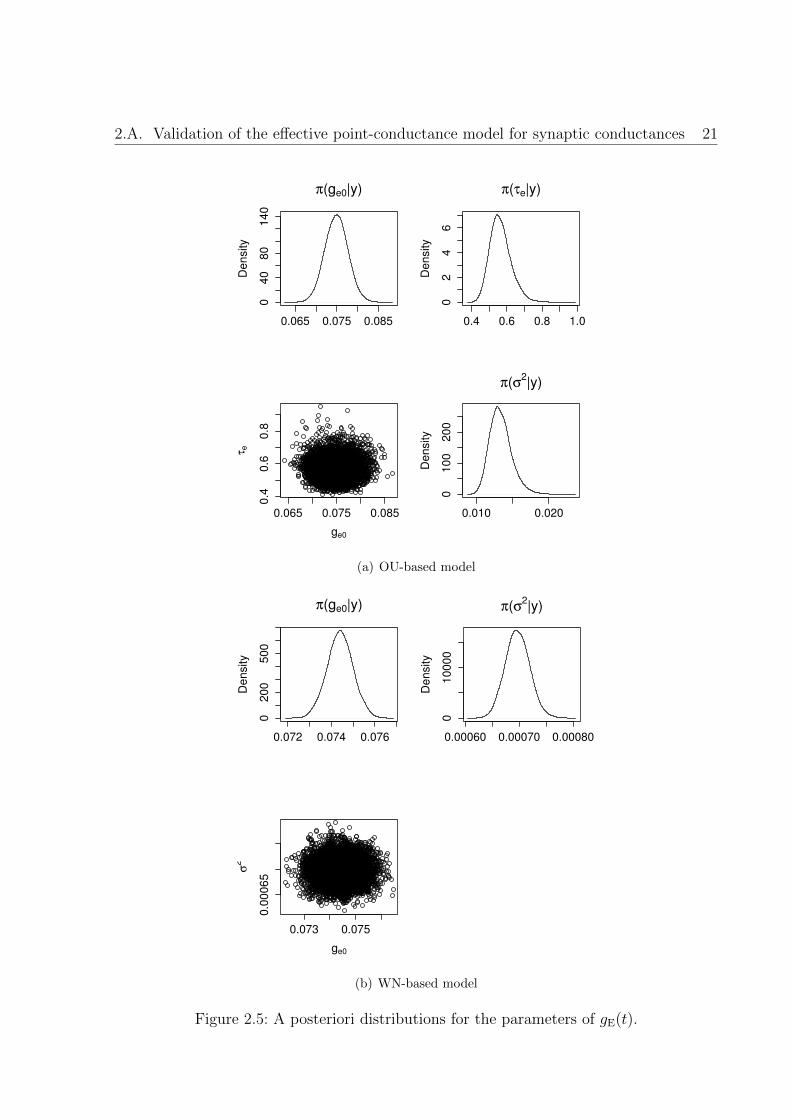
2.5 A posteriori distributions for the parameters of gE(t). . . . . . . . . . . . . 21
2.6 A posteriori distributions for the parameters of gI(t). . . . . . . . . . . . . 22
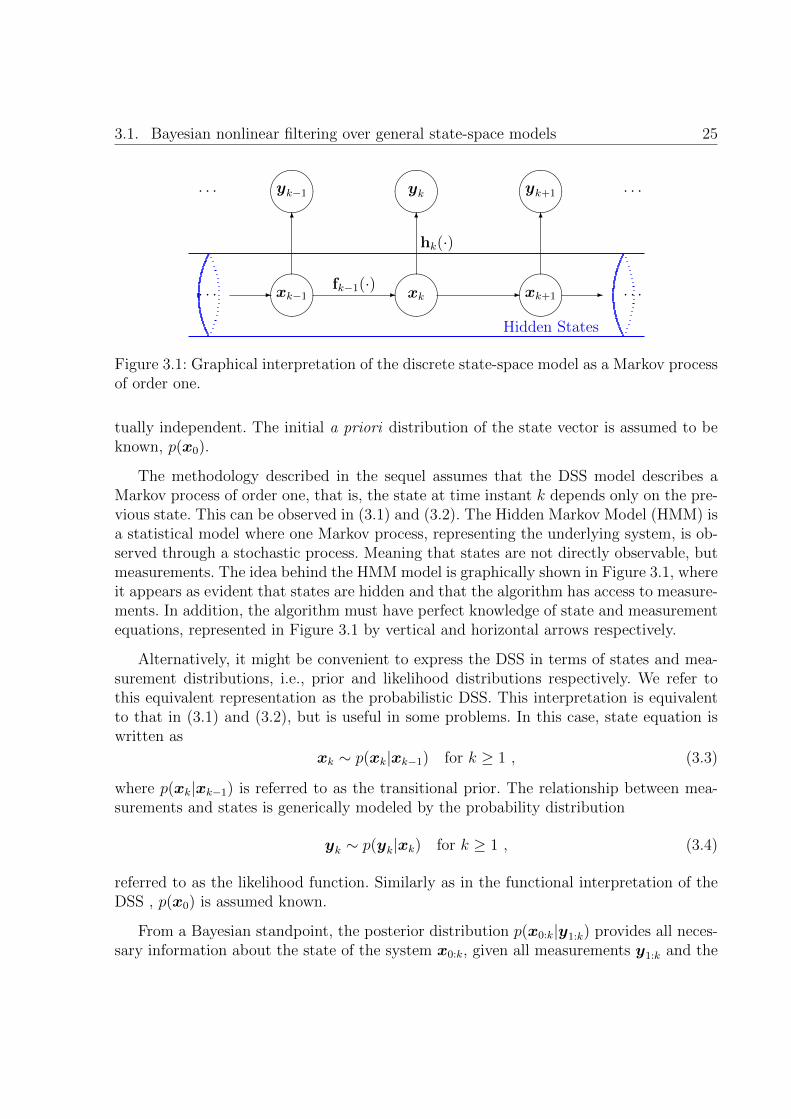
3.1 Graphical interpretation of the discrete state-space model as a Markovprocess of order one. . . . . . . . . . . . . . . . . . . . . . . . . . . . . . . 25
3.2 Dimensionality growth of the Trajectory Information Matrix with k. . . . . 31
4.1 Evolution of the RMSE and the PCRB over time. Model inaccuracies whereσI = 0.01 · Io and σgL = 0.01 · goL. . . . . . . . . . . . . . . . . . . . . . . . 73
4.2 Evolution of the RMSE and the PCRB over time. Model inaccuracies whereσI = 0.1 · Io and σgL = 0.1 · goL. . . . . . . . . . . . . . . . . . . . . . . . . . 74
4.3 A single realization of the particle filtering method for SNR = 0 dB (left)and SNR = 32 dB (right). . . . . . . . . . . . . . . . . . . . . . . . . . . . 75
4.4 Realizations of the PMCMC algorithm for joint state-parameter estima-tion. Each plot corresponds to different unknown parameters, featuring theMCMC iterations (top) that converge to the true value of the parameterand the filtered voltage trace (bottom). . . . . . . . . . . . . . . . . . . . . 81
4.5 Evolution of RMSE(vk) (top) and RMSE(nk) (bottom) over time for thePMCMC method estimating the leakage parameters. Model inaccuracieswhere σI = 0.1 · Io and σgL = 0.1 · goL. . . . . . . . . . . . . . . . . . . . . . 82
xv
4.6 Parameter estimation performance of the proposed PMCMC algorithm.Top plots show results for gL = 2 estimation and bottom plots for EL =−60. Left plots show superimposed independent realizations and right plotsthe average estimate of the parameter. . . . . . . . . . . . . . . . . . . . . 83
4.7 A single realization of the PF method with perfect model knowledge, es-timating voltage and gating variables (top) and synaptic conductances innS (bottom). . . . . . . . . . . . . . . . . . . . . . . . . . . . . . . . . . . 84
4.8 A single realization of the PMCMC method, estimating voltage and gatingvariables (top) and synaptic conductances in nS (bottom) as well as modelparameters. . . . . . . . . . . . . . . . . . . . . . . . . . . . . . . . . . . . 85
xvi
Notation
Boldface upper-case letters denote matrices and boldface lower-case letters denote columnvectors.
R, C The set of real and complex numbers, respectively.
RN×M , CN×M The set of N ×M matrices with real- and complex-valued entries,respectively.
x Estimation and true value of parameter x.
f(x)|x=a Function f(x) evaluated at x = a.
|x| Absolute value (modulus) of scalar x.
‖x‖ `2-norm of vector x, defined as ‖x‖ =(xHx
) 12 .
dimx Dimension of vector x.
[x]r The r-th vector element.
[X]r,c The matrix element located in row r and column c.
[X]r,: The r-th row of matrix X.
[X]:,c The c-th column of matrix X.
TrX Trace of matrix X. TrX =N∑n=1
[X]nn.
det(X) Determinant of matrix X.
diag(x) A diagonal matrix whose diagonal entries are given by x.
‖X‖F Frobenius norm of matrix X. If X is N ×N ,
‖X‖F =
(N∑u=1
N∑v=1
|xuv|2) 1
2
=(TrXHX
) 12
Chol (A) Cholesky factorization of an Hermitian positive-definite matrix Asuch that A = SS> if S = Chol (A).
xvii
I Identity matrix. A subscript can be used to indicate the dimension.
X∗ Complex conjugate of matrix X (also applied to scalars).
XT Transpose of matrix X.
XH Complex conjugate and transpose (Hermitian) of matrix X.
X† Moore-Penrose pseudoinverse of matrix X. If X is M ×N ,
X† = XH(XXH
)−1if M ≤ N ,
X† = X−1 if M = N , and
X† =(XHX
)−1XH if M ≥ N .
Schur-Hadamard (elementwise) product of matrices.If A and B are two N ×M matrices:
AB =
a11b11 a12b12 · · · a1Mb1M
a21b21 a22b22. . . a2Mb2M
...... . . .
...aN1bN1 aN2bN2 · · · aNMbNM
⊗ The Kronecker or tensor product. If A is m× n, then
A⊗B =
[A]11B · · · [A]1mB...
...[A]n1B · · · [A]nmB
PX Orthogonal projector onto the subspace spanned by the columns of X.
PX = X(XHX
)−1XH .
P⊥X I−PX, orthogonal projector onto the orthogonal complementto the columns of X.
N (µ,Σ) Multivariate Gaussian distribution with mean µ and covariance matrix Σ.
U(a, b) Uniform distribution in the interval [a, b].
E · Statistical expectation. When used with a subindex, it specifiesthe distribution over which the expectation is taken, e.g.,Ex · over the distribution of a random variable x;Ex,y · over the joint distribution of x and y, p(x, y);Ex|y · over the distribution of x conditioned to y, p(x|y).
ln(·) Natural logarithm (base e).
δ(n−m) Kronecker’s delta function, defined as:
δ(n−m) = δn,m ,
1, if n = m0, if n 6= m
xviii
<·, =· Real and imaginary parts, respectively.
op(fN) A sequence of random variables XN is XN = op(fN), for fN > 0 ∀N ,when XN
fNconverges to zero in probability, i.e.,
limN→∞
P
∣∣∣∣XN
fN
∣∣∣∣ > δ
= 0 ∀δ > 0
f(t) ∗ g(t) Convolution between f(t) and g(t).
arg maxx
f(x) Value of x that maximizes f(x).
arg minxf(x) Value of x that minimizes f(x).
∂f(x)∂xi
Partial derivative of function f(x) with respect to the variable xi.∂f(x)∂x
Gradient of function f(x) with respect to vector x.
∂2f(x)∂x2 Hessian matrix of function f(x) with respect to vector x.
∇xf(x) Gradient of function f(x) with respect to vector x.
Hxf(x) Hessian matrix of function f(x) with respect to vector x.
4x2x1f(x) second-order partial derivatives operator of function f(x) with
respect to vectors x1 and x2. Notice that Hxf(x) , 4xxf(x)
and 4x2x1
= ∇x1
[∇T
x2
].
f(t), f(t) derivatives of t ime of function f(t), equivalent to ∂f(t)∂t
and ∂2f(t)∂t2
respectively.
a.s. almost surely convergence.
i.i.d. independent identically distributed.
q.e.d. quod erat demonstrandum.
r.v. random variable.
w.p.1. convergence with probability one.
xix

xx
Acronyms
ADC Analog-to-Digital Converter.
AMPA α-amino-3-hydroxy-5-methyl-4-isoxazolepropionic.
AR autoregressive.
AWGN Additive White Gaussian Noise.
BIM Bayesian Information Matrix.
BLUE Best Linear Unbiased Estimator.
CKF cubature Kalman filter.
CNS Central Nervous System.
CRB Cramer Rao Bound.
DSS discrete state-space.
EKF extended Kalman filter.
EM Expectation Maximization algorithm.
FIM Fisher Information Matrix.
GABA γ-aminobutyric acid.
HMM Hidden Markov Model.
IS Importance Sampling.
QKF quadrature Kalman filter.
KF Kalman filter.
LS Least Squares.
ODE ordinary differential equation.
OU Ornstein-Uhlenbeck.
MAP Maximum a posteriori.
MCMC Markov-Chain Monte-Carlo.
ML Maximum Likelihood.
MLE Maximum Likelihood Estimator.
xxi
MMSE Minimum Mean Square Error.
MSE Mean Square Error.
PCRB Posterior Cramer-Rao Bound.
PDF Probability Density Function.
PF particle filter.
PMCMC particle Markov-Chain Monte-Carlo.
RAM Robust Adaptive Metropolis.
RMSE root mean square error.
SIR Sampling Importance Resampling.
SIS Sequential Importance Sampling.
SMC Sequential Monte-Carlo.
SNR Signal to Noise Ratio.
SPKF sigma–point Kalman filter.
SRUKF square–root unscented Kalman filter.
SRCKF square–root cubature Kalman filter.
SRQKF square–root quadrature Kalman filter.
SRKF square–root Kalman filter.
SRSPKF square–root sigma–point Kalman filter.
SS state-space.
UKF unscented Kalman filter.
UT unscented transform.
xxii
1Introduction
THIS dissertation deals with the problem of inferring the signals and parameters thatcause neural activity to occur. The focus is on a microscopic vision of the problem,
where single-neuron models (potentially connected to a network of peers) are in the coreof the Thesis. The sole observation available are noisy, sampled voltage traces obtainedfrom intracellular recordings. We design algorithms and inference methods using the toolsprovided by Bayesian filtering, that allow a probabilistic interpretation and treatment ofthe problem.
In this chapter, we glance at the structure of the document, serving as a guide to thereader. For the sake of clarity, the mathematical notation and the acronyms used alongthe dissertation can be consulted at the beginning of the document.
1.1 Motivation and Objectives of the Thesis
One of the most challenging problems in neuroscience is to unveil brain’s connectivity. Thisproblem might be treated from several perspectives, here we focus on the local phenomenaoccurring at a single neuron. The ultimate goal is thus to understand the dynamics ofneurons and how the interconnection with other neurons affects its state.
1
2 Chapter 1. Introduction
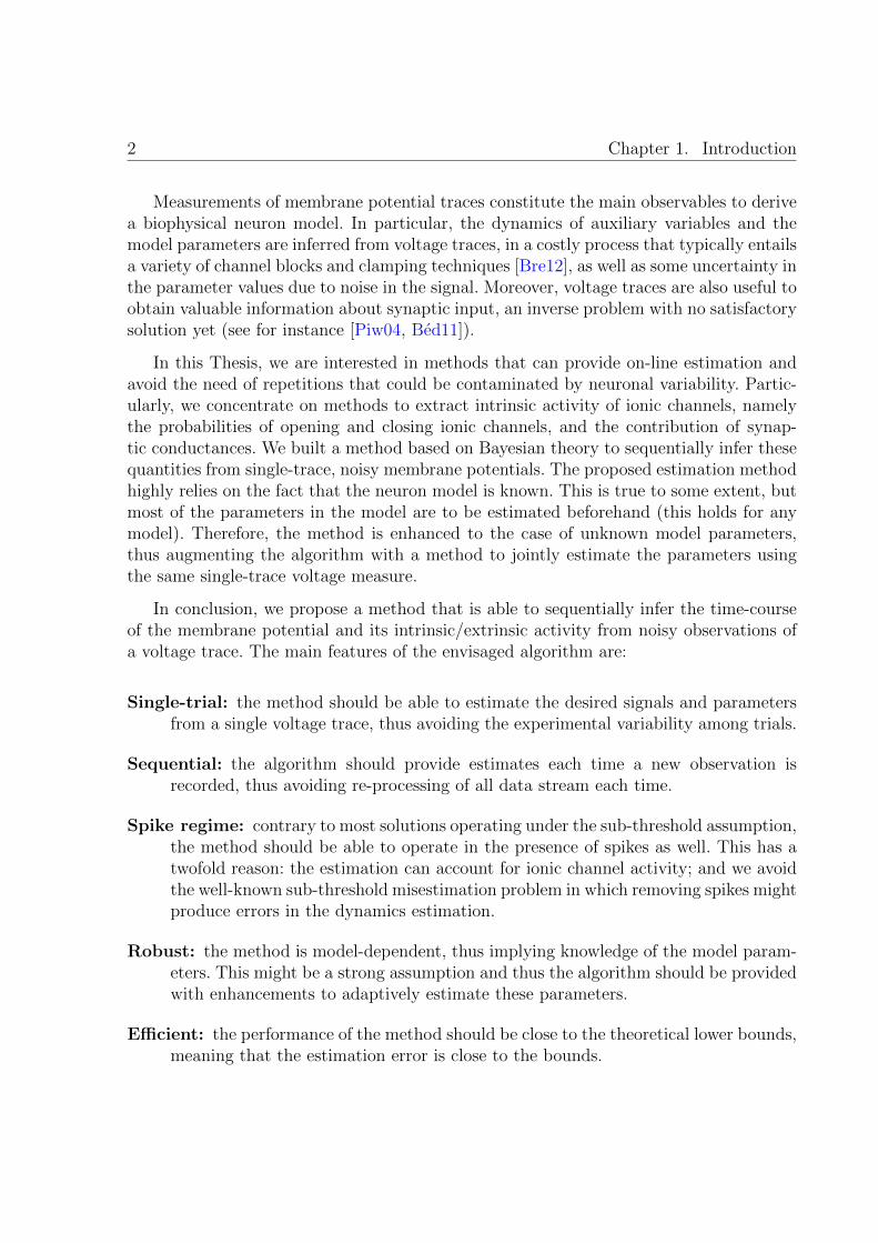
Measurements of membrane potential traces constitute the main observables to derivea biophysical neuron model. In particular, the dynamics of auxiliary variables and themodel parameters are inferred from voltage traces, in a costly process that typically entailsa variety of channel blocks and clamping techniques [Bre12], as well as some uncertainty inthe parameter values due to noise in the signal. Moreover, voltage traces are also useful toobtain valuable information about synaptic input, an inverse problem with no satisfactorysolution yet (see for instance [Piw04, Bed11]).
In this Thesis, we are interested in methods that can provide on-line estimation andavoid the need of repetitions that could be contaminated by neuronal variability. Partic-ularly, we concentrate on methods to extract intrinsic activity of ionic channels, namelythe probabilities of opening and closing ionic channels, and the contribution of synap-tic conductances. We built a method based on Bayesian theory to sequentially infer thesequantities from single-trace, noisy membrane potentials. The proposed estimation methodhighly relies on the fact that the neuron model is known. This is true to some extent, butmost of the parameters in the model are to be estimated beforehand (this holds for anymodel). Therefore, the method is enhanced to the case of unknown model parameters,thus augmenting the algorithm with a method to jointly estimate the parameters usingthe same single-trace voltage measure.
In conclusion, we propose a method that is able to sequentially infer the time-courseof the membrane potential and its intrinsic/extrinsic activity from noisy observations ofa voltage trace. The main features of the envisaged algorithm are:
Single-trial: the method should be able to estimate the desired signals and parametersfrom a single voltage trace, thus avoiding the experimental variability among trials.
Sequential: the algorithm should provide estimates each time a new observation isrecorded, thus avoiding re-processing of all data stream each time.
Spike regime: contrary to most solutions operating under the sub-threshold assumption,the method should be able to operate in the presence of spikes as well. This has atwofold reason: the estimation can account for ionic channel activity; and we avoidthe well-known sub-threshold misestimation problem in which removing spikes mightproduce errors in the dynamics estimation.
Robust: the method is model-dependent, thus implying knowledge of the model param-eters. This might be a strong assumption and thus the algorithm should be providedwith enhancements to adaptively estimate these parameters.
Efficient: the performance of the method should be close to the theoretical lower bounds,meaning that the estimation error is close to the bounds.
1.2. Thesis Outline and Reading Directions 3
Notice that the focus in this Thesis is not on computational reduction techniques, aswe thought that other requirements (like performance) were prioritized in this application.The results show the validity of the approach and its statistical efficiency. Although weused the Morris-Lecar neuron model in the computer simulations, the proposed procedurecan be applied to any neuron model without loss of generality.
1.2 Thesis Outline and Reading Directions
The dissertation consists of 5 Chapters, where review material and novel contributionsare presented. The thesis might be of interest to two groups of people: those working inthe neuroscience field and to signal-processing oriented researchers with the objective oflearning new fancy applications. The document is organized according to this premise,providing the basics of each topic. For the sake of clarity, the main ideas of the chaptersare summarized herein:
Chapter 1 This chapter summarizes the main problem addressed and our research objec-tives for the rest of the Thesis. We provide as well the reader with reading directions.
Chapter 2 Basic material on neuroscience is provided for the non-specialist to get thebiophysical meaning of the problem addressed. From the vast amount of informationon the numerous disciplines related to neuroscience, we focus on a microscopic visionwhere single-neuron models are the core concept. In the chapter we sketch the basicmodeling procedures to mimic neuron dynamics.
Note: if you have expertise in neuroscience you can skip this chapter, and pleaseforgive me for the rather vague introduction.
Chapter 3 Similarly to the neuroscience material in Chapter 2, we provide a textbookreview of Bayesian filtering methodology. The reason being its paramount impor-tance in the derivation of the type of algorithms we are interested in this Thesis. Ata glance, we present the theoretical Bayesian solution to recursive filtering and detailthe most popular algorithms and go beyond what is strictly necessary for the com-prehension of the methods derived in Chapter 4. We also comment on the derivationof theoretical estimation bounds under this framework, which is not always tackledin the literature where neuroscience and Bayesian filtering collide.
Note: if you know what a Kalman filter or a particle filter is you might be temptedto skip this chapter, please do it.
Chapter 4 This constitutes the core chapter in the Thesis. The material therein includesdiscussion of the discrete state-space representation of the problem and the model
4 Chapter 1. Introduction
inaccuracies due to missmodeling effects. In this chapter we present 2 sequentialinference algorithms: i) a method based on particle filtering to estimate the time-evolving states of a neuron under the assumption of perfect model knowledge; andii) an enhanced version where model parameters are jointly estimated, and thusthe rather strong assumption of perfect model knowledge is relaxed. We provideexhaustive computer simulation results to validate the algorithms and observe thatthey are consistent, in the sense of attaining the theoretical lower bounds derivedin the chapter as well.
Chapter 5 This concluding chapter summarizes the main results obtained in this Thesisand points out some interesting open problems which constitute the future workafter the Thesis defence.
The work presented in this Thesis has been partially published in the form of scientificpublications and talks. We list them here.
[1] C. Vich, P. Closas, and A. Guillamon, “Data treatment in estimating synaptic con-ductances: wrong procedures and new proposals,” Barcelona Computational and SystemsNeuroscience (BARCSYN), June 16 and 17, 2014.
[2] P. Closas, A. Guillamon, “Estimation of neural voltage traces and associated vari-ables in uncertain models,” BMC Neuroscience, Vol. 14, No. 1, pp. 1151, July 2013.
[3] P. Closas, A. Guillamon, “Estimation of neural voltage traces and associated vari-ables in uncertain models,” in Proceedings of the 22nd Annual Computational Neuro-science Meeting (CNS 2013), 13-18 July 2013, Paris (France).
[4] P. Closas, A. Guillamon, “Sequential estimation of gating variables from voltagetraces in single-neuron models by particle filtering,” in Proceedings of IEEE InternationalConference on Acoustics, Speech and Signal Processing (ICASSP 2013) 26-31 May 2013,Vancouver (Canada).
[5] P. Closas, and A. Guillamon, “Inference of voltage traces and gating variables inuncertain models,” Barcelona Computational and Systems Neuroscience (BARCSYN),June 13 and 14, 2013.
2Fundamentals of Neuroscience
NEUROSCIENCE is the science that delves into the understanding of the nervous sys-tem. It is one of the most interdisciplinary sciences, gathering together experts from
a vast variety of fields of knowledge including biology, chemistry, medicine, psychology,physics, mathematics, statistics, engineering, and computer science.
Neuroscience is a rather broad discipline and encompasses many aspects related tothe Central Nervous System (CNS). The different topics in neuroscience can be stud-ied from various perspectives depending on the prism used to focus the problem. Thisranges from understanding the internal mechanisms that cause a single cell (a neuron) tospike, to explaining the dynamics occurring in populations of neurons that are intercon-nected. Going further, more macroscopic analysis are important like those treating poolsof neuron as an anatomically meaningful function. From microscopic to macroscopic, theCNS research could be classified into molecular neuroscience, cellular neuroscience, neuralcircuits, systems neuroscience, and cognitive neuroscience.
This Thesis deals with single neuron models, with the rest of the Chapter being devotedto explaining the basic ideas behind a neuron physiology and related mathematical models.Recommended textbooks are [Day05, Izh06, Kee09] and more recently [Erm10], fromwhich we extracted part of the material presented in this chapter.
5

6 Chapter 2. Fundamentals of Neuroscience
Figure 2.1: Diagram of a neuron (Source: http://en.wikipedia.org/wiki/Neuron).
2.1 Electrophysiology of neurons
Neurons are the basic information processing structures in the CNS. The main functionof a neuron is to receive input information from other neurons, to process that informa-tion, and to send output information to other neurons. Synapses are connections betweenneurons, through which they communicate this information. It is controversial how thisinformation is encoded, but it is quite accepted that information produces changes in theelectrical activity of the neurons, seen as voltage changes in the membrane potential (i.e.,the difference in electrical potential between the interior and the exterior of a biologicalcell).
To put some numbers, the human brain has only around 1011 neurons and 1015 con-nections among them (a.k.a. synapses). The basic constituents of a neuron can be seen inFig. 2.1, where we can identify:
Soma: contains the nucleus of the cell, it is the body of the neuron where most of theinformation processing is carried.
Dendrites: are extensions of the soma which connect the neuron to neighboring neurons.Dendrites are capturing the stimuli from the rest of neurons.
Axon: is the largest part of a neuron where the information is transmitted in form ofan electrical current. A cell might have only one axon or more. The physiologicalmeaning for the propagation of the voltage through the axon can be understood
2.2. Ionic currents 7
in terms of voltage-gated ionic channels located in the axon membrane. This isparamount in the topic treated in this Thesis, and thus we provide some furtherdetails in this section.
Synapses: located at the axon terminal, are in charge of the electrochemical reactionsthat cause neuron communications to happen. More precisely, the membrane poten-tial (electrical phenomena) traveling through the axon, when reaching the synapse,activates the emission of neurotransmitters (chemical phenomena) from the neuronto the receptors of the target neurons. This chemical reaction is transformed againinto electrical impulses in the dendrites of the receiving neurons.
2.2 Ionic currents
We are specially interested in understanding the phenomena through which an electricalvoltage travels the axon from the soma to the synapse. We concentrate here on the bio-physical meaning and its mathematical modeling. The basic idea is that the membranecovering the axon is essentially impermeable to most charged molecules. This makes theaxon to act as a capacitor (in terms of electrical circuits) that separates the inner andouter parts of the neuron’s axon. This is combined with the so-called ionic-channels, thatallow the exchange of intracellular/extracellular ions through electrochemical gradients.This exchange of ions is responsible for the generation of an electrical pulse called actionpotential, that travels along the neuron’s axon. Ionic-channels are found throughout theaxon and are typically voltage-dependent, which is primarily how the action potentialpropagates.
The most common ionic species involves in the generation of the action potentialare sodium (Na+), potassium (K+), chloride (Cl−), and calcium (Ca2+). For each ionicspecies, the corresponding ionic-channel aims at balancing the concentration and electricalpotential gradients, which are opposite forces regulating the exchange of ions throughthe gate. The point at which both forces counterbalance is known as Nernst equilibriumpotential and given by
Eion ≈ 62 log10
[Ion]out
[Ion]in(2.1)
in mV, where [Ion]out and [Ion]in are the concentrations of the ion inside and outsidethe cell, respectively. Nernst equilibrium potential is value for which the cross-membranepotential is zero for a given ionic channel. In the sequel, we denote by ENa, EK, ECl, andECa the Nernst equilibrium potential of the typical ionic species. The time-varying netcurrent of the i-th ionic species, i ∈ I = Na,K,Cl,Ca, . . . , is thus
Ii = gI(v − Ei) (2.2)
8 Chapter 2. Fundamentals of Neuroscience
where gI , gI(t) is the time-varying conductance of the ionic channel in mS/cm2, and(v − Ei) is the driving force that zeroes when the voltage is equal to the equilibriumpotential as argued earlier. The time dependent conductances are responsible for spike(or action potential) generation.
2.3 Conductance-based models
The voltage travels through the axon over time, which results in the so-called compartmen-tal neuron models. For the sake of simplicity and without loss of generality, we considerthe evolution of the membrane potential at a specific site of the axon. Therefore, v , v(t)denotes the continuous-time membrane potential at a point in the axon. Accounting thatthe membrane potential is seen as a capacitor, the current-voltage relation allows us toexpress the total current flowing in the membrane as proportional to the time derivativeof the voltage. Then, we have that the mathematical model for the evolution of membranepotentials is of the basic form
Cmv = −∑i∈I
Ii − gL(v − EL)− Isyn + Iapp (2.3)
where Cm is the membrane capacitance and Iapp represents the externally applied currents,for instance injected via an electrode and used to perform a controlled experiment.
In (2.3) we have introduced two additional terms. The first one is referred to as theleakage term. The leakage is mathematically used to gather all ionic channels that are notexplicitly modeled. The maximal conductance of the leakage, gL, is considered constantand it is adjusted to match the membrane potential at resting state. Similarly, EL has tobe estimated at rest. The second new term in (2.3) gathers the contribution of neighboringneurons and it is referred to as the synaptic current, Isyn. We will see later how to modelthe synaptic current.
Strictly speaking, (2.3) is a dynamical system, although we have to provide moredetails for the different components before using it as a reliable model for neural activity.There are several models [Izh04, Izh06] that explain the membrane potential evolutionusing dynamical systems theory. Roughly speaking, there are terms which model intrinsicactivity of the neuron (mostly, chemical reactions in the cell) and terms related to thecontribution of synaptic noise to the neuron’s activity (that is the voltages received fromneighboring neurons) [Hod52, Piw04, Bed11, Kob11, Bre12]. Section 2.4 comments on theformer mechanisms, mainly discussing the ionic conductances.
Ionic channels are the responsible for electrochemical gradient stabilization of ionicspecies. The conductance of the i-th channel, gi, can be seen as a switch that opens or

2.3. Conductance-based models 9
closes the pump. Recall that i ∈ I = Na,K,Cl,Ca, . . . . A refinement of (2.2) is then,
Ii = gi pi(v − Ei) (2.4)
where gi is a constant called the maximal conductance, which is fixed for each ionic species.The variable pi , pi(v) is the average proportion of channels of the type i in the openstate. Notice that the proportion is in general voltage-dependent (i.e., sensitive to themembrane potential) and thus they are said to be voltage-gated.
The proportion pi can be further classified into gates that activate (i.e., gates thatopen the i-th ionic channel) and those that inactivate (i.e., gates that close the i-th ionicchannel). Mathematically, omitting the dependence on i,
p = mahb (2.5)
where a is the number of activation gates and 0 < m , mi(v) < 1 the probability ofactivating gate being in the open state. Similarly, b is the number of inactivation gatesand 0 < h , hi(v) < 1 the probability of inactivating gate being in the open state.
We refer to m and h as the gating variables of the ionic channel. The dynamics ofthese gating variables are responsible for the membrane potential generation and can beexpressed by a first-order differential equation:
m =m∞(v)−m
τm(v)(2.6)
h =h∞(v)− hτh(v)
(2.7)
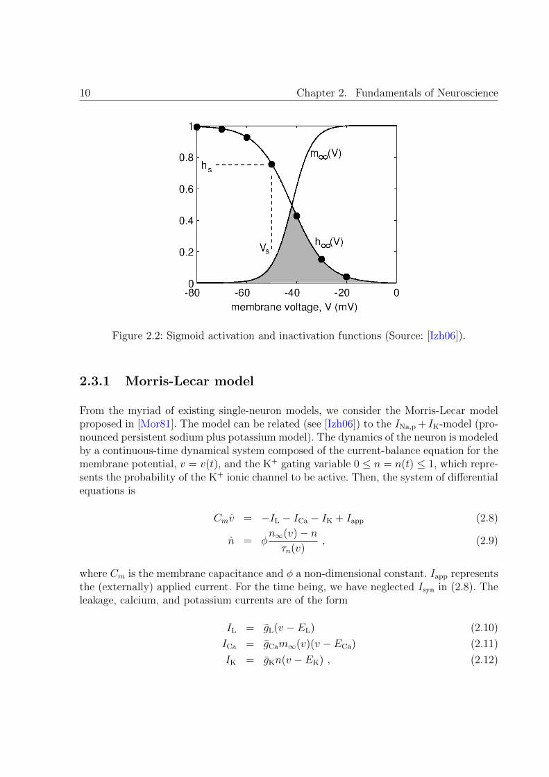
where the activation/inactivation functions (m∞(v) and h∞(v), respectively) and timeconstants (τm(v) and τm(v)) can be measured experimentally. The activation and inacti-vation functions are typically a sigmoid. The parameters defining the sigmoids are thenrelated to the type of gate. As seen in Fig. 2.2, for large membrane potentials activatinggates are more likely to be open. Conversely for inactivating gates. The time constantsresemble a Gaussian, and smaller values of the time constant imply faster dynamics ofthe corresponding gating variable.
As a result, we have seen that neural activity can be modeled as a system of differentialequations. Precisely, one for the voltage as in (2.3), and then as many first-order differentialequations as gating variables and ionic channels. In the literature one might find manymodels following the basic formulae in (2.3) and (2.4), mostly varying on the number andtype of gating variables and the activation/inactivation functions defining the dynamicsof the gating variables. The pioneer work by [Hod52] has been followed by a plethora ofalternative models such as [Mor81, Fit61, Nag62, Izh04]. Without loss of generality, inthe sequel we consider one of the most popular single-neuron models: the Morris-Lecarmodel, which is introduced in the following section.
10 Chapter 2. Fundamentals of Neuroscience
Figure 2.2: Sigmoid activation and inactivation functions (Source: [Izh06]).
2.3.1 Morris-Lecar model
From the myriad of existing single-neuron models, we consider the Morris-Lecar modelproposed in [Mor81]. The model can be related (see [Izh06]) to the INa,p + IK-model (pro-nounced persistent sodium plus potassium model). The dynamics of the neuron is modeledby a continuous-time dynamical system composed of the current-balance equation for themembrane potential, v = v(t), and the K+ gating variable 0 ≤ n = n(t) ≤ 1, which repre-sents the probability of the K+ ionic channel to be active. Then, the system of differentialequations is
Cmv = −IL − ICa − IK + Iapp (2.8)
n = φn∞(v)− nτn(v)
, (2.9)
where Cm is the membrane capacitance and φ a non-dimensional constant. Iapp representsthe (externally) applied current. For the time being, we have neglected Isyn in (2.8). Theleakage, calcium, and potassium currents are of the form
IL = gL(v − EL) (2.10)
ICa = gCam∞(v)(v − ECa) (2.11)
IK = gKn(v − EK) , (2.12)
2.4. Synaptic inputs 11
respectively. gL, gCa, and gK are the maximal conductances of each current. EL, ECa, andEK denote the Nernst equilibrium potentials, for which the corresponding current is zero,a.k.a. reverse potentials.
The dynamics of the activation variable m is considered at the steady state, and thuswe write m = m∞(v). On the other hand, the time constant τn(v) for the gating variablen cannot be considered that fast and the corresponding differential equation needs to beconsidered. The formulae for these functions is
m∞(v) = 12· (1 + tanh[v−V1
V2]) (2.13)
n∞(v) = 12· (1 + tanh[v−V3
V4]) (2.14)
τn(v) = 1/(cosh[v−V32V4
]) , (2.15)
which parameters V1, V2, V3, and V4 can be measured experimentally [Izh06].
The knowledgeable reader would have noticed that the Morris-Lecar model is aHodgin-Huxley type-model with the usual considerations, where the following two ex-tra assumptions were made: the depolarizing current is generated by Ca2+ ionic channels(or Na+ depending on the type of neuron modeled), whereas hyperpolarization is carriedby K+ ions; and that m = m∞(v). The Morris-Lecar model is very popular in computa-tional neuroscience as it models a large variety of neural dynamics while its phase-planeanalysis is more manageable as it involves only two states [Rin98].
The Morris Lecar, although simple to formulate, results in a very interesting modelas it can produce a number of different dynamics. For instance, for given values of itsparameters, we encounter a subcritic Hopf bifurcation for Iapp = 93.86 µA/cm2. On theother hand, for another set of parameter values, the system of equations has a Saddle-Nodeon an Invariant Circle (SNIC) bifurcation at Iapp = 39.96 µA/cm2.
2.4 Synaptic inputs
The synaptic current, Isyn, gathers the contribution of neighboring neurons. Isyn is re-sponsible for activating spike generation in neurons, without externally applying currents(e.g., via Iapp). The most general model for Isyn considers decomposition in 2 independentcomponents:
Isyn = gE(t)(v(t)− EE) + gI(t)(v(t)− EI) (2.16)
corresponding to excitatory (α-amino-3-hydroxy-5-methyl-4-isoxazolepropionic (AMPA)neuroreceptors) and inhibitory (γ-aminobutyric acid (GABA) neuroreceptors) terms, re-spectively. Roughly speaking, whereas the excitatory synaptic term makes the postsynap-tic neuron more likely to generate a spike, the inhibitory term makes the postsynaptic
12 Chapter 2. Fundamentals of Neuroscience
neuron less likely to generate an action potential. EE and EI are the corresponding reversepotentials. A longstanding problem is to characterize the time-varying global excitatoryand inhibitory conductances gE(t) and gI(t). We present here 3 mathematical models forthe synaptic current.
1. A classical model is to consider each of the 2 synapses as a whole, gathering thecontributions of all the synapses of that type. In this case, similarly as for thevoltage-dependent conductances, the synaptic conductance can be written as theproduct of its maximal conductance (gu) and the channel open probability (pu),
gu(t) = gupu (2.17)
where u = E, I. In turn, pu = suru can be expressed in terms of the processoccurring on the pre- and post-synaptic sides: the probability that a postsynapticchannel is open state (su) and the probability that a transmitter is released bythe pre-synaptic terminal (r). A simple model for su is similar to the model foropening/closing gating variables:
su = αu(1− su)− βusu (2.18)
where αu and βu are the opening and closing rates of the channel u, respectively.
2. A further refinement of the above is to account for multiple postsynaptic channels.Particularly, if NE and NI denote the total number of excitatory and inhibitorysynapses, then a plausible model is
Isyn =
NE∑nE=1
gAMPAm(nE)E (t)(v(t)− EE) +
NI∑nI=1
gGABAm(nI)I (t)(v(t)− EI) (2.19)
where gAMPA and gGABA are maximal conductances, and m(n)u (t) is the fraction of
open post-synaptic receptors of the type u at each individual synapse n for a giventime t. The kinetic equations for these variable are very similar to those in (2.18)with corresponding parameters. Notice that these individual dynamics differ in thetime constant, defined by 1/αu. This model is realistic, although might be intractablefor estimation and simulation purposes if the number of synapses increases.
3. A third alternative is fundamentally different, it is referred to as effective point-conductance model in [Rud03, Piw04]. In this model, the excitatory/inhibitoryglobal conductances are treated as Ornstein-Uhlenbeck (OU) processes
gu(t) = − 1
τu(gu(t)− gu,0) +
√2σ2
u
τuχ(t) (2.20)
2.5. Intracellular recordings 13
where χ(t) is a zero-mean, white noise, Gaussian process with unit variance. Then,the OU process has mean gu,0, standard deviation σu, and time constant τu. Recallthat we used the notation u = E, I. Although this is a much simpler model than(2.19), it was shown in [Rud03] that the OU model yields to a valid description ofsynaptic noise, capturing the properties of the more complex model.
Estimation of the synaptic conductances and its parameters is one of the main chal-lenges in modern neuroscience. There is a lack for efficient algorithms able to estimatethese quantities on-line, from a single trial, and robustly adapting to model uncertainties.These are goals addressed in this Thesis.
2.5 Intracellular recordings
The membrane potential, obtained from intracellular recordings, is one of the most valu-able signals of neurons’ activity. Most of the neuron models have been derived from finemeasurements and allow the progress of “in silico” experiments. The recording of themembrane potential is a physical process, which involves two main issues not taken intoaccount in the ideal model (2.3):
1. Voltage observations are noisy. This is due to the thermal noise at the sensing device,non-ideal conditions in experimental setups, etc.
2. Recorded observations are discrete. All sensing devices record data by sampling atregular time intervals the continuous-time natural phenomena. This is the task of anAnalog-to-Digital Converter (ADC). Moreover, these samples are typically digitized,i.e. expressed by a finite number of bits. This latter issue is not tackled in the Thesisas we assume that modern computer capabilities allow us to sample with relativelylarge number of bits per sample.
Therefore, the problem investigated in this Thesis considers recordings of noisy voltagetraces to infer the hidden gating variables of the neuron model, as well as filtered voltageestimates. Data is recorded at discrete time-instants k at a sampling frequency fs = 1/Ts.The problem can thus be posed in the form of a discrete-time, state-space model. Theobservations are
yk ∼ N (vk, σ2y,k) , (2.21)
with σ2y,k modeling the noise variance due to the sensor or the instrumentation inaccuracies
when performing the experiment. To provide comparable results, we define the signal-to-noise ratio (SNR) as SNR = Ps/Pn, with Ps being the average signal power and Pn = σ2
y,k
the noise power.
14 Chapter 2. Fundamentals of Neuroscience
Neuron
Excitatory pool Inhibitory pool
gI(t)gE(t)
v(t)
Sensing Devicenoisy, sampled version of v(t)
yk
Hidden System
Inference methods recover:- Time-evolving states (membrance potential and gating variables)
- Unknown model parameters
- Synaptic conductances.
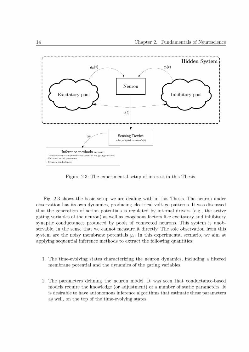
Figure 2.3: The experimental setup of interest in this Thesis.
Fig. 2.3 shows the basic setup we are dealing with in this Thesis. The neuron underobservation has its own dynamics, producing electrical voltage patterns. It was discussedthat the generation of action potentials is regulated by internal drivers (e.g., the activegating variables of the neuron) as well as exogenous factors like excitatory and inhibitorysynaptic conductances produced by pools of connected neurons. This system is unob-servable, in the sense that we cannot measure it directly. The sole observation from thissystem are the noisy membrane potentials yk. In this experimental scenario, we aim atapplying sequential inference methods to extract the following quantities:
1. The time-evolving states characterizing the neuron dynamics, including a filteredmembrane potential and the dynamics of the gating variables.
2. The parameters defining the neuron model. It was seen that conductance-basedmodels require the knowledge (or adjustment) of a number of static parameters. Itis desirable to have autonomous inference algorithms that estimate these parametersas well, on the top of the time-evolving states.
2.6. Summary 15
3. The dynamics of synaptic conductances and its parameters. The final goal being toDiscern the temporal contributions of global excitation from those of global inhibi-tion, gE(t) and gI(t) respectively.
2.6 Summary
In this chapter, we gained some insight on the biological components of a neuron and theproblem we aim at addressing. We presented conductance-based models for single-neurons,the biophysical meaning of its parameters, and explained in more detail a particular modelnamed after Morris and Lecar. Without loss of generality, the latter model is used alongthe Thesis to validate the algorithms. In this discussion we left integrate-and-fire modelson purpose [Izh06], although the methodology followed in the Thesis could be applied aswell. Finally, we briefly sketched the practical implications of working with intracellularrecords which, basically, imply that observations are noisy and sampled.
16 Chapter 2. Fundamentals of Neuroscience
Appendix 2.A Validation of the effective point-
conductance model for synaptic con-
ductances
This Appendix validates the OU model introduced in Section 2.4 with a set of realisticconductance measures. To do so we apply the tools from Bayesian modeling.
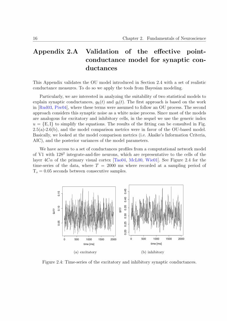
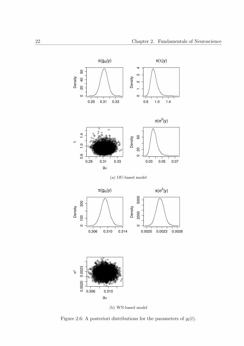
Particularly, we are interested in analyzing the suitability of two statistical models toexplain synaptic conductances, gE(t) and gI(t). The first approach is based on the workin [Rud03, Piw04], where these terms were assumed to follow an OU process. The secondapproach considers this synaptic noise as a white noise process. Since most of the modelsare analogous for excitatory and inhibitory cells, in the sequel we use the generic indexu = E, I to simplify the equations. The results of the fitting can be consulted in Fig.2.5(a)-2.6(b), and the model comparison metrics were in favor of the OU-based model.Basically, we looked at the model comparison metrics (i.e. Akaike’s Information Criteria,AIC), and the posterior variances of the model parameters.
We have access to a set of conductances profiles from a computational network modelof V1 with 1282 integrate-and-fire neurons, which are representative to the cells of thelayer 4Cα of the primary visual cortex [Tao04, McL00, Wie01]. See Figure 2.4 for thetime-series of the data, where T = 2000 ms where recorded at a sampling period ofTs = 0.05 seconds between consecutive samples.
0 500 1000 1500 2000
0.0
50
.10
0.1
5
time [ms]
ge(t
)
(a) excitatory
0 500 1000 1500 2000
0.2
00.2
50.3
00.3
50.4
00.4
5
time [ms]
gi(
t)
(b) inhibitory
Figure 2.4: Time-series of the excitatory and inhibitory synaptic conductances.
2.A. Validation of the effective point-conductance model for synaptic conductances 17
2.A.1 Synaptic conductances as an Ornstein-Uhlenbeck process
According to [Rud03, Piw04], a OU process is reasonable for the modeling of synaptic noiseand has similar properties to more detailed (and thus complex) models. This appendixseeks validation of this statement. The OU process, in its discrete version using Euler’smethod, can be expressed
gu,k+1 = gu,k −Ts
τu(gu,k − gu,0) + Ts
√2σ2
u
τuχ (2.22)
where χ is a zero-mean, independent white noise, Gaussian process with unit variance.Then, the OU process has mean gu,0, standard deviation σu, and time constant τu.
The model in (2.22) can be rearranged as the following linear/Gaussian model:
gu,k+1 = βu0 + βu1gu,k + σχ (2.23)
which is more convenient for the model fitting purposes we aim at. In (2.23) we defined:
βu0 = 1− Ts
τu(2.24)
βu1 = Tsgu0
τu(2.25)
σ = Ts
√2σ2
u
τu. (2.26)
The observed data are the time-series of gE(t) and gI(t) that we plotted in Figure 2.4.Therefore, we can define a vector of observations as
ge = (gE,1, . . . , gE,T )> (2.27)
gi = (gI,1, . . . , gI,T )> (2.28)
and the vectors of explanatory variables as
xe = (0, gE,1, . . . , gE,T−1)> (2.29)
xi = (0, gI,1, . . . , gI,T−1)> , (2.30)
then, the model in (2.23) can be expressed in vector form and we come up with anstatistical model such as:
M1 = gu|βu0, βu1, τ ∼ N (βu0 + βu1xu, τI), (βu0, βu1, τ) ∈ R3+ , (2.31)
18 Chapter 2. Fundamentals of Neuroscience
with I being the n×n identity matrix, and τ.= σ−2 the precision of the normal distribution
(we are using WinBUGS notation here).
For the Bayesian model to be completed, we need to set a priori distributions for eachof the unknown quantities in the statistical model M1, we select:
βu0 ∼ π(βu0) = N (0, 10−5) (2.32)
βu1 ∼ π(βu1) = N (0, 10−5) (2.33)
τ ∼ π(τ) = Γ(10−3, 10−3) . (2.34)
Finally, it is worth mentioning that we are able to recover the desired parameters of theOU model by undoing the transformations. It is straightforward to see from (2.24)–(2.26)that
τu =Ts
1− βu1
(2.35)
gu0 =βu0
1− βu1
(2.36)
σu =1
2τTs
1
(1− βu1), (2.37)
and it is even easier to obtain the a posteriori distributions of each parameter with Win-BUGS (see code below).
The chunk of WinBUGS code implementing the OU model is:
model
# statistical model:
for ( i in 1:N)
y[i] ~ dnorm(mu[i], tau.y)
E[i] <- y[i]- mu[i]
E2[i] <- pow(E[i], 2)
mu[1] <- b0
for ( j in 2:N)
mu[j] <- b1*x[j] + b0
# a priori distributions:
2.A. Validation of the effective point-conductance model for synaptic conductances 19
b0 ~ dnorm(0, 0.00001)
b1 ~ dnorm(0, 0.00001)
tau.y ~ dgamma(0.001, 0.001)
# obtaining the desired parameters:
tau <- Ts/(1-b1)
g0 <- b0/(1-b1)
sigma2 <- 1/(2*tau.y*Ts*(1-b1))
SQE <- sum(E2[])
2.A.2 Synaptic conductances as a white noise process
At the light of the time-series in Figure 2.4, one could be tempted to model the synapticconductances as a white noise process of the form:
gu,k = αu0 + σuχ (2.38)
where χ is a zero-mean, white noise, Gaussian process with unit variance. The model hastwo unknown quantities αu0 and σ2
u. Therefore, the statistical model might be describedin this case as:
M2 = gu|αu0, τ ∼n∏i=1
N (αu0, τ.= σ−2
u ), (αu0, τ) ∈ R2+ (2.39)
where we assumed i.i.d. observations. We chose the a priori distributions
αu0 ∼ π(αu0) = N (0, 10−5) (2.40)
τ ∼ π(τ) = Γ(10−3, 10−3) . (2.41)
The chunk of WinBUGS code implementing the WN model is:
model
# statistical model:
for ( i in 1:N)
y[i] ~ dnorm(a0, tau.y)
20 Chapter 2. Fundamentals of Neuroscience
#E[i] <- y[i]- a0
#E2[i] <- pow(E[i], 2)
# a priori distributions:
a0 ~ dnorm(0, 0.00001)
tau.y ~ dgamma(0.001, 0.001)
# obtaining the desired parameters:
sigma2 <- 1/tau.y
#SQE <- sum(E2[])
2.A. Validation of the effective point-conductance model for synaptic conductances 21
0.065 0.075 0.085
04
08
01
40
π(ge0|y)
De
nsity
0.4 0.6 0.8 1.0
02
46
π(τe|y)
De
nsity
0.065 0.075 0.085
0.4
0.6
0.8
ge0
τe
0.010 0.020
01
00
20
0
π(σ2|y)
De
nsity
(a) OU-based model
0.072 0.074 0.076
0200
500
π(ge0|y)
Density
0.00060 0.00070 0.00080
010000
π(σ2|y)
Density
0.073 0.075
0.0
0065
ge0
σ2
(b) WN-based model
Figure 2.5: A posteriori distributions for the parameters of gE(t).
22 Chapter 2. Fundamentals of Neuroscience
0.29 0.31 0.33
020
40
60
π(gi0|y)
Density
0.6 1.0 1.4
01
23
4
π(τi|y)
Density
0.29 0.31 0.33
0.6
1.0
1.4
gi0
τi
0.03 0.05 0.07
020
60
π(σ2|y)
Density
(a) OU-based model
0.306 0.310 0.314
01
00
30
0
π(gi0|y)
De
nsity
0.0020 0.0023 0.0026
02
00
05
00
0
π(σ2|y)
De
nsity
0.306 0.3100.0
02
00
.00
23
gi0
σ2
(b) WN-based model
Figure 2.6: A posteriori distributions for the parameters of gI(t).
3Fundamentals of Bayesian Filtering
THE type of problems we are interested in involve the estimation of time-evolving pa-rameters that can be expressed through a state-space (SS) formulation. Particularly,
estimation of the states in a single-neuron model from noisy voltage traces can be readilyseen as a filtering (even smoothing) problem. Bayesian theory provides the mathematicaltools to deal with such problems in a systematic manner following the axioms of probabil-ity. The focus is on sequential methods that can incorporate new available measurementsas they are recorded data without the need for reprocessing all past measurements. Thisis accomplished by the Bayesian filtering methodology and the related algorithms.
Ultimately, in Bayes theory we are interested in computing the marginal posteriordistribution of having the system in a state xk at discrete time k after observing datafrom 1 to k, that is p(xk|y1, . . . ,yk). For instance, in the case of the Morris-Lecar modelthe states are the values of voltage traces and the gating variable.
This chapter presents an introductory overview on the optimal filtering frameworkand the algorithms that a practitioner has at hand. More precisely, we have organized theChapter as follows. First, the optimal Bayesian filtering framework is presented in Section3.1. Then, Section 3.2 reviews fundamental estimation bounds of filtering methods andSection 3.3 briefly sketches the algorithms one can use to implement Bayesian filtersdepending on the type of system under study. We have included an appendix with moredetails on the particle filtering methodology, which is of paramount importance in this
23
24 Chapter 3. Fundamentals of Bayesian Filtering
Thesis since methods designed in Chapter 4 are based on this approach. The details onthe rest of algorithms are given here for the sake of completeness.
3.1 Bayesian nonlinear filtering over general state-
space models
In general, the natural way to account for prior information is to consider a SS model. TheSS representation provides a twofold modeling. On the one han, state equation illustratesthe evolution of states with time. In other words, state equation mathematically expressesthe prior information that the algorithm has regarding the state1. On the other hand,measurement equation models the dependency of measurements with unknown states. Inthis section, we introduce the general discrete state-space (DSS) model and the Bayesianconceptual solution, which is only analytically tractable when some assumptions hold.The section discusses both optimal and state-of-the-art suboptimal algorithms to obtainthe Bayesian solution. We restrict ourselves to the discrete version of the SS model sinceit is the one required along this dissertation. Although similar, the continuous SS modelhas its own particularities that an interested reader can explore in detail in [And79].
3.1.1 Considering Prior information: the Bayesian recursion
The DSS approach deals with the nonlinear filtering problem: recursively compute esti-mates of states xk ∈ Rnx given measurements yk ∈ Cny at time index k based on allavailable measurements, y1:k = y1, . . . ,yk. State equation models the evolution in timeof target states as a discrete-time stochastic model, in general
xk = fk−1(xk−1,νk) , (3.1)
where fk−1(·) is a known, possibly nonlinear, function of the state xk and νk is referredto as process noise which gathers any mismodeling effect or disturbances in the statecharacterization. In our case, for instance, fk−1(·) is defined by the ordinary differentialequations (ODEs) describing the Morris-Lecar model where xk includes the voltage tracesand the gating variable. The relation between measurements and states is modeled by
yk = hk(xk, ek) , (3.2)
where hk(·) is a known possibly nonlinear function and ek is referred to as measurementnoise. Both process and measurement noise are assumed with known statistics and mu-
1We understand by state the evolving (vector) r.v. that drives measurements and which is the esti-mation objective.
3.1. Bayesian nonlinear filtering over general state-space models 25
· · · -xk−1 -
6
fk−1(·)
xk -
6
hk(·)
xk+1 -
6
· · ·
· · · yk−1
yk
yk+1 · · ·
Hidden States
Figure 3.1: Graphical interpretation of the discrete state-space model as a Markov processof order one.
tually independent. The initial a priori distribution of the state vector is assumed to beknown, p(x0).
The methodology described in the sequel assumes that the DSS model describes aMarkov process of order one, that is, the state at time instant k depends only on the pre-vious state. This can be observed in (3.1) and (3.2). The Hidden Markov Model (HMM) isa statistical model where one Markov process, representing the underlying system, is ob-served through a stochastic process. Meaning that states are not directly observable, butmeasurements. The idea behind the HMM model is graphically shown in Figure 3.1, whereit appears as evident that states are hidden and that the algorithm has access to measure-ments. In addition, the algorithm must have perfect knowledge of state and measurementequations, represented in Figure 3.1 by vertical and horizontal arrows respectively.
Alternatively, it might be convenient to express the DSS in terms of states and mea-surement distributions, i.e., prior and likelihood distributions respectively. We refer tothis equivalent representation as the probabilistic DSS. This interpretation is equivalentto that in (3.1) and (3.2), but is useful in some problems. In this case, state equation iswritten as
xk ∼ p(xk|xk−1) for k ≥ 1 , (3.3)
where p(xk|xk−1) is referred to as the transitional prior. The relationship between mea-surements and states is generically modeled by the probability distribution
yk ∼ p(yk|xk) for k ≥ 1 , (3.4)
referred to as the likelihood function. Similarly as in the functional interpretation of theDSS , p(x0) is assumed known.
From a Bayesian standpoint, the posterior distribution p(x0:k|y1:k) provides all neces-sary information about the state of the system x0:k, given all measurements y1:k and the

26 Chapter 3. Fundamentals of Bayesian Filtering
prior p(x0:k). The Bayes’ theorem allows to express the posterior in terms of the likelihoodand prior distributions:
p(x0:k|y1:k) =p(y1:k|x0:k)p(x0:k)
p(y1:k), (3.5)
which can be written as
p(x0:k|y1:k) =p(x0)
∏kt=1 p(yt|xt)p(xt|xt−1)
p(y1:k)(3.6)
where we take into account that measurements are independent given x0:k and considerthe Markov state evolution depicted in Figure 3.1.
We are interested in the marginal distribution p(xk|y1:k) since, as will be seen laterin this section, it allows the estimation of the realization of the target state vector xk.p(xk|y1:k) can be obtained by marginalization of (3.6), being the dimension of the integralgrowing with k. Alternatively the desired density2 can be computed sequentially in twostages: prediction and update. The basic idea is to, assuming the filtering distributionknown at k− 1, first predict the new state and then incorporate the new measurement toobtain the distribution at k:
· · · −→ p(xk−1|y1:k−1) −→ p(xk|y1:k−1)︸ ︷︷ ︸prediction
−→ p(xk|y1:k)︸ ︷︷ ︸update
−→ · · ·
First we notice from (3.6) that the posterior distribution can be recursively expressedas:
p(x0:k|y1:k) =p(yk|xk)p(xk|xk−1)
p(yk|y1:k−1)p(x0:k−1|y1:k−1) , (3.7)
where the marginal p(xk|y1:k) also satisfies the recursion [Sor88]. Given that p(x0) ,p(x0|y0) is known, where y0 is the set of no measurements, we can assume that therequired density at time k − 1 is available, p(xk−1|y1:k−1). In the prediction stage thepredicted distribution is obtained by considering that p(xk|xk−1,y1:k−1) = p(xk|xk−1),due to the first-order Markovian SS model considered. Using the Chapman-Kolmogorovequation (see Appendix 3.A) to remove xk−1 we obtain,
p(xk|y1:k−1) =
∫p(xk|xk−1)p(xk−1|y1:k−1)dxk−1 . (3.8)
2In the sequel, p(xk|y1:k) is referred to as the filtering distribution. In contrast to p(x0:k|y1:k), whichis the posterior distribution.
3.1. Bayesian nonlinear filtering over general state-space models 27
Whenever a new measurement becomes available at instant k, the predicted distribu-tion in (3.8) is updated via the Bayes’ rule (see Appendix 3.A)
p(xk|y1:k) = p(xk|yk,y1:k−1)
=p(yk|xk,y1:k−1)p(xk|y1:k−1)
p(yk|y1:k−1)
=p(yk|xk)p(xk|y1:k−1)
p(yk|y1:k−1), (3.9)
being the normalizing factor
p(yk|y1:k−1) =
∫p(yk|xk)p(xk|y1:k−1)dxk . (3.10)
Now the recursion is enclosed by equations (3.8) and (3.9), assuming some knowledgeabout the state evolution and the relation between measurements and states, describedby p(xk|xk−1) and p(yk|xk) respectively. This recursion form the basis of the optimalBayesian solution.
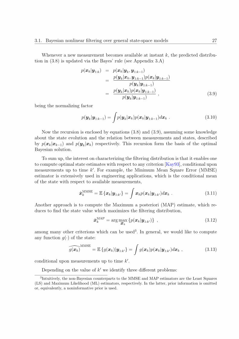
To sum up, the interest on characterizing the filtering distribution is that it enables oneto compute optimal state estimates with respect to any criterion [Kay93], conditional uponmeasurements up to time k′. For example, the Minimum Mean Square Error (MMSE)estimator is extensively used in engineering applications, which is the conditional meanof the state with respect to available measurements,
xMMSEk = E xk|y1:k′ =
∫xkp(xk|y1:k′)dxk . (3.11)
Another approach is to compute the Maximum a posteriori (MAP) estimate, which re-duces to find the state value which maximizes the filtering distribution,
xMAPk = arg max
xkp(xk|y1:k′) , (3.12)
among many other criterions which can be used3. In general, we would like to computeany function g(·) of the state:
g(xk)MMSE
= E g(xk)|y1:k′ =
∫g(xk)p(xk|y1:k′)dxk , (3.13)
conditional upon measurements up to time k′.
Depending on the value of k′ we identify three different problems:
3Intuitively, the non-Bayesian counterparts to the MMSE and MAP estimators are the Least Squares(LS) and Maximum Likelihood (ML) estimators, respectively. In the latter, prior information is omittedor, equivalently, a noninformative prior is used.
28 Chapter 3. Fundamentals of Bayesian Filtering
Smoothing. It is the case of k′ > k, were the state x0:k is estimated using future mea-surements.
Filtering. Corresponds to the case k′ = k. It is the problem considered in the sequel andthe approach that is followed along the dissertation.
Prediction. In this case, one predicts values of states with measurements of previousinstants: k′ < k.
What the reader has read so far, corresponds to the conceptual solution of Bayesianfiltering (smoothing and prediction) that is endowed with the sequential equations (3.8)and (3.9). In some particular cases, the recursion can be solved analytically and thusoptimally. However, in general it cannot be solved and thus we need to resort to suboptimalalgorithms. The most popular alternatives are discussed in Section 3.3. Before delving intothe details of Bayesian filters, we devote Section 3.2 to understand the computation oftheoretical lower bounds on estimation accuracy. The latter is of paramount importanceto establish benchmarks and comparison among different estimation algorithms.
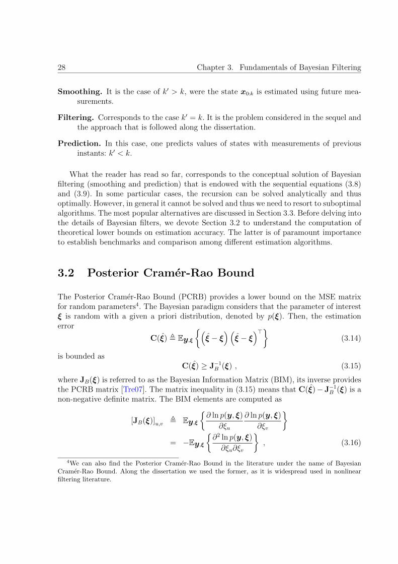
3.2 Posterior Cramer-Rao Bound
The Posterior Cramer-Rao Bound (PCRB) provides a lower bound on the MSE matrixfor random parameters4. The Bayesian paradigm considers that the parameter of interestξ is random with a given a priori distribution, denoted by p(ξ). Then, the estimationerror
C(ξ) , Ey,ξ(ξ − ξ
)(ξ − ξ
)>(3.14)
is bounded asC(ξ) ≥ J−1
B (ξ) , (3.15)
where JB(ξ) is referred to as the Bayesian Information Matrix (BIM), its inverse providesthe PCRB matrix [Tre07]. The matrix inequality in (3.15) means that C(ξ)− J−1
B (ξ) is anon-negative definite matrix. The BIM elements are computed as
[JB(ξ)]u,v , Ey,ξ∂ ln p(y, ξ)
∂ξu
∂ ln p(y, ξ)
∂ξv
= −Ey,ξ
∂2 ln p(y, ξ)
∂ξu∂ξv
, (3.16)
4We can also find the Posterior Cramer-Rao Bound in the literature under the name of BayesianCramer-Rao Bound. Along the dissertation we used the former, as it is widespread used in nonlinearfiltering literature.
3.2. Posterior Cramer-Rao Bound 29
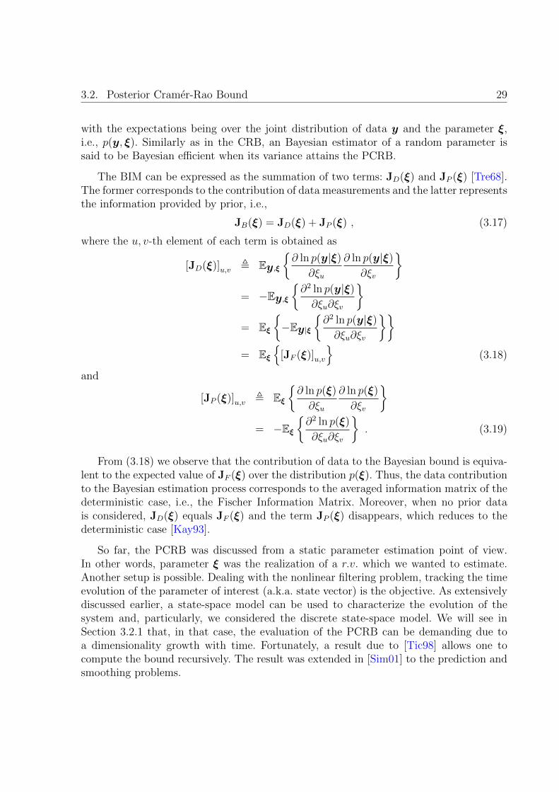
with the expectations being over the joint distribution of data y and the parameter ξ,i.e., p(y, ξ). Similarly as in the CRB, an Bayesian estimator of a random parameter issaid to be Bayesian efficient when its variance attains the PCRB.
The BIM can be expressed as the summation of two terms: JD(ξ) and JP (ξ) [Tre68].The former corresponds to the contribution of data measurements and the latter representsthe information provided by prior, i.e.,
JB(ξ) = JD(ξ) + JP (ξ) , (3.17)
where the u, v-th element of each term is obtained as
[JD(ξ)]u,v , Ey,ξ∂ ln p(y|ξ)
∂ξu
∂ ln p(y|ξ)
∂ξv
= −Ey,ξ
∂2 ln p(y|ξ)
∂ξu∂ξv
= Eξ
−Ey|ξ
∂2 ln p(y|ξ)
∂ξu∂ξv
= Eξ
[JF (ξ)]u,v
(3.18)
and
[JP (ξ)]u,v , Eξ
∂ ln p(ξ)
∂ξu
∂ ln p(ξ)
∂ξv
= −Eξ
∂2 ln p(ξ)
∂ξu∂ξv
. (3.19)
From (3.18) we observe that the contribution of data to the Bayesian bound is equiva-lent to the expected value of JF (ξ) over the distribution p(ξ). Thus, the data contributionto the Bayesian estimation process corresponds to the averaged information matrix of thedeterministic case, i.e., the Fischer Information Matrix. Moreover, when no prior datais considered, JD(ξ) equals JF (ξ) and the term JP (ξ) disappears, which reduces to thedeterministic case [Kay93].
So far, the PCRB was discussed from a static parameter estimation point of view.In other words, parameter ξ was the realization of a r.v. which we wanted to estimate.Another setup is possible. Dealing with the nonlinear filtering problem, tracking the timeevolution of the parameter of interest (a.k.a. state vector) is the objective. As extensivelydiscussed earlier, a state-space model can be used to characterize the evolution of thesystem and, particularly, we considered the discrete state-space model. We will see inSection 3.2.1 that, in that case, the evaluation of the PCRB can be demanding due toa dimensionality growth with time. Fortunately, a result due to [Tic98] allows one tocompute the bound recursively. The result was extended in [Sim01] to the prediction andsmoothing problems.
30 Chapter 3. Fundamentals of Bayesian Filtering
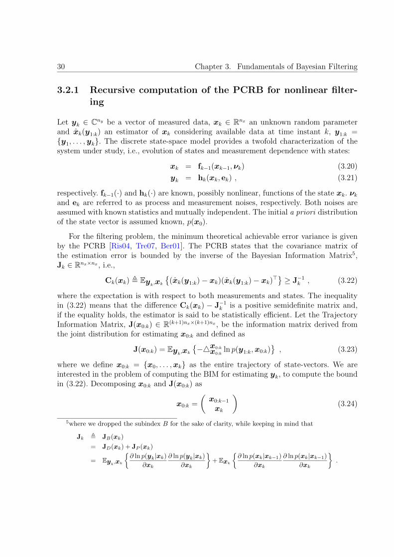
3.2.1 Recursive computation of the PCRB for nonlinear filter-ing
Let yk ∈ Cny be a vector of measured data, xk ∈ Rnx an unknown random parameterand xk(y1:k) an estimator of xk considering available data at time instant k, y1:k =y1, . . . ,yk. The discrete state-space model provides a twofold characterization of thesystem under study, i.e., evolution of states and measurement dependence with states:
xk = fk−1(xk−1,νk) (3.20)
yk = hk(xk, ek) , (3.21)
respectively. fk−1(·) and hk(·) are known, possibly nonlinear, functions of the state xk. νkand ek are referred to as process and measurement noises, respectively. Both noises areassumed with known statistics and mutually independent. The initial a priori distributionof the state vector is assumed known, p(x0).
For the filtering problem, the minimum theoretical achievable error variance is givenby the PCRB [Ris04, Tre07, Ber01]. The PCRB states that the covariance matrix ofthe estimation error is bounded by the inverse of the Bayesian Information Matrix5,Jk ∈ Rnx×nx , i.e.,
Ck(xk) , Eyk,xk
(xk(y1:k)− xk)(xk(y1:k)− xk)>≥ J−1
k , (3.22)
where the expectation is with respect to both measurements and states. The inequalityin (3.22) means that the difference Ck(xk) − J−1
k is a positive semidefinite matrix and,if the equality holds, the estimator is said to be statistically efficient. Let the TrajectoryInformation Matrix, J(x0:k) ∈ R(k+1)nx×(k+1)nx , be the information matrix derived fromthe joint distribution for estimating x0:k and defined as
J(x0:k) = Eyk,xk−4x0:k
x0:kln p(y1:k,x0:k)
, (3.23)
where we define x0:k = x0, . . . ,xk as the entire trajectory of state-vectors. We areinterested in the problem of computing the BIM for estimating yk, to compute the boundin (3.22). Decomposing x0:k and J(x0:k) as
x0:k =
(x0:k−1
xk
)(3.24)
5where we dropped the subindex B for the sake of clarity, while keeping in mind that
Jk , JB(xk)
= JD(xk) + JP (xk)
= Eyk,xk
∂ ln p(yk|xk)
∂xk
∂ ln p(yk|xk)
∂xk
+ Exk
∂ ln p(xk|xk−1)
∂xk
∂ ln p(xk|xk−1)
∂xk
.

3.2. Posterior Cramer-Rao Bound 31
k = 1
J1
J(x0:1)
k = 2
J2
J(x0:2)
k = 3
J3
J(x0:3)
k = 4
J4
J(x0:4)
Figure 3.2: Dimensionality growth of the Trajectory Information Matrix with k.
and
J(x0:k) =
(Ak Bk
B>k Ck
)(3.25)
,
Eyk,xk−4x0:k−1
x0:k−1ln p(y1:k,x0:k)
Eyk,xk
−4xkx0:k−1
ln p(y1:k,x0:k)
Eyk,xk−4x0:k−1
xk ln p(y1:k,x0:k)
Eyk,xk−4xkxk ln p(y1:k,x0:k)
,
respectively, we can compute the PCRB, J−1k ∈ Rnx×nx , as the lower-right corner of
J−1(x0:k), i.e.,
Jk = Ck −B>k A−1k Bk . (3.26)
Notice that the computation of the nx × nx BIM involves either the inversion of Ak ∈Rknx×knx or the inversion of J−1(x0:k). Clearly, this can imply a high computational cost.
As depicted in Figure 3.2, the dimensionality of J(x0:k) grows with k. This poses acomputational problem to the computation of the PCRB, which conveys the idea of deriv-ing a recursive computation of the bound. Some papers proposed to relate the nonlinearfiltering problem to an equivalent linear system, e.g., [Bob75]. However, the problem ispartially solved in these approaches and still the recursion was to be found by [Tic98].The latter provides a recipe for computing Jk without manipulating large matrices, suchas J(x0:k). Proposition 3.1 states the main result of that work.
Proposition 3.1. The sequence Jk of posterior information submatrices for estimatingstate vectors xk can be obtained using the following recursion:
Jk+1 = D22k −D21
k
(Jk + D11
k
)−1D12k , (3.27)

32 Chapter 3. Fundamentals of Bayesian Filtering
where
D11k = Exk,xk+1
−4xkxk ln p(xk+1|xk)
D12k = Exk,xk+1
−4xk+1
xk ln p(xk+1|xk)
D21k = Exk,xk+1
−4xkxk+1
ln p(xk+1|xk)
=[D12k
]>D22k = Exk,xk+1
−4xk+1
xk+1ln p(xk+1|xk)
+ Exk+1,yk+1
−4xk+1
xk+1ln p(yk+1|xk+1)
(3.28)
and the initialization is done considering the prior density of the states:
J0 = Ex0
−4x0
x0ln p(x0)
. (3.29)
Proof. See Appendix 3.B.
The recursion in (3.27) is extremely useful in many cases where the computation ofthe PCRB is mathematically untractable. In addition, matrices involved in the recursiveformula are nx× nx, in contrast to the problem in equation (3.23) which has a dimensionthat increases with k (see Figure 3.2).
When the general DSS model described by (3.20) and (3.21) is particularized, somesimplifications apply to the recursive computation of the PCRB in (3.27) and (3.28). Therest of the section is devoted to present those particularizations.
a) Additive Gaussian noise
In this case, the general DSS model is expressed as:
xk = fk−1(xk−1) + νk
yk = hk(xk) + ek , (3.30)
where both process and measurement noise are zero-mean and Gaussian distributed, withcovariance matrices being Σx,k and Σy,k respectively. Then, we have that
− ln p(xk+1|xk) = c1 +1
2(xk+1 − fk(xk))
>Σ−1x,k (xk+1 − fk(xk)) (3.31)
− ln p(yk+1|xk+1) = c2 +1
2
(yk+1 − hk+1(xk+1)
)>Σ−1y,k+1
(yk+1 − hk+1(xk+1)
),
3.2. Posterior Cramer-Rao Bound 33
where c1 and c2 are constants, and
D11k = Exk
F>k Σ−1
x,kFk
D12k = −Exk
F>k
Σ−1x,k
D22k = Σ−1
x,k + Exk+1
H>k+1Σ
−1y,k+1Hk+1
. (3.32)
In (3.32) we use the definitions of Jacobian of hk(xk) and hk(xk) evaluated at the truevalue of xk:
Hk =[∇xkh>k (xk)
]>Fk =
[∇xkf>k (xk)
]>, (3.33)
respectively.
The difficulty in evaluating (3.32) comes due to the need of performing the expectationover xk and xk+1. The common approach is to approximate such expectations usingMonte-Carlo simulation, i.e., create a significative number of state-vector trajectories,calculate the corresponding PCRB and average them to obtain the theoretical PCRB ofthe system under study. In certain cases, where the process noise is small, the expectationcan be dropped out as a good approximation.
b) Linear systems under additive Gaussian noise
The linear DSS model corrupted by additive Gaussian noise reduces to :
xk = Fk−1xk−1 + νk
yk = Hkxk + ek , (3.34)
where Fk−1 and Hk are known matrices that represent linear functions, referred to astransitional and measurement matrices respectively. νk and ek are mutually independentrandom variables drawn from a zero-mean white Gaussian probability density functionwith known covariance matrices, Σx,k and Σy,k respectively.
In this case, it is straightforward to show that the recursion can be expressed as:
Jk+1 = Σ−1x,k −Σ−1
x,kFk
(Jk + F>k Σ−1
x,kFk
)−1F>k Σ−1
x,k + H>k+1Σ−1y,k+1Hk+1 , (3.35)
and using the matrix inversion lemma
Jk+1 =(Σx,k + F>k J−1
k Fk
)−1+ H>k+1Σ
−1y,k+1Hk+1 (3.36)
we obtain an expression with two terms: one corresponds to the process prediction andthe other to the measurement update.
34 Chapter 3. Fundamentals of Bayesian Filtering
c) Linear states and nonlinear measurements under additive Gaussian noise
Consider a DSS model as:
xk = Fk−1xk−1 + νk
yk = hk(xk) + ek , (3.37)
where the previous definitions hold. Some simplifications apply to (3.32 under that DSSmodel. Considering that states are drawn from a Gaussian pdf and p(x0) = N (x0,Σx,0),after mathematical manipulation of equation (3.29) we obtain that J0 = Σ−1
x,0. In addition,
D11k = F>k Σ−1
x,kFk
D12k = −F>k Σ−1
x,k
D22k = Σ−1
x,k + Exk+1
H>k+1Σ
−1y,k+1Hk+1
, (3.38)
where we use the definitions in (3.33). Notice that, after simplifications due to the modelat hand, matrices D11
k , D12k and D21
k are deterministic and can be easily obtained. How-ever, due to the non-linearity in the measurement model, the expectation operator inthe computation of D22
k cannot be dropped out. In order to compute this expectation, aMonte-Carlo approximation can be performed as previously commented.
d) Nonlinear states and linear measurements under additive Gaussian noise
Consider a DSS model as:
xk = fk−1(xk−1) + νk
yk = Hkxk + ek , (3.39)
where the transition equation is nonlinear/Gaussian and the measurements are expressedas a linear/Gaussian equation. Using (3.33), the components of the recursive PCRB for-mulation are
D11k = Exk
F>k Σ−1
x,kFk
D12k = −Exk
F>k
Σ−1x,k
D22k = Σ−1
x,k + H>k+1Σ−1y,k+1Hk+1 . (3.40)
where we D22k becomes deterministic, but the rest of terms involving expectations have
to be computed by Monte Carlo approximations.
This last case is the situation we will face in this Thesis: noisy/linear observations ofstates with nonlinear state evolution, everything under the Gaussian assumption.
3.3. Algorithms implementing Bayesian filtering 35
3.3 Algorithms implementing Bayesian filtering
There are few cases where the Bayesian filtering problem can be analytically solved. Animportant case is when the system can be considered linear and Gaussian, in which casethe Kalman filter (KF) [Kal60, And79] is known to be optimal. Another interesting caseis when the SS is discrete and finite, where the optimal solution exists and can be foundvia optimal grid based methods [Ris04].
In more general models one must resort to suboptimal algorithms. A number of meth-ods can be found in the literature [Che03]. A popular tool are particle filters (PFs)[Dou01a, Aru02, Dju03, Ris04] , a set of simulation-based methods which are applica-ble in very general nonlinear/non-Gaussian setups. Another appealing class of filters iscomposed of those variants of the KF which could operate with nonlinearities under theGaussian assumption: extended Kalman filter (EKF) [And79, Kay93], unscented Kalmanfilter (UKF) [Jul97, Jul00, Wan00], central difference filter (CDF) [Ito00], divided differ-ence filter (DDF) [Nor00], quadrature Kalman filter (QKF) [Ara08], or cubature Kalmanfilter (CKF) [Ara09]. Due to the Gaussian assumption, these algorithms only require theestimation of the first two moments of the distribution. They basically differ in the waythey perform this estimation. Unlike the EKF, where only mean and covariance are prop-agated through the nonlinearity by means of a linearization process, the rest of mentionedKF–like algorithms resort to a set of so-called sigma-points to efficiently characterize thepropagation of the normal distribution over the nonlinear system. Therefore, these filtersare referred to with the general term of sigma–point Kalman filters (SPKFs) [Mer03]. Inthis section, we review the most popular Bayesian filtering algorithms.
3.3.1 The Kalman filter
Nobody can question that the KF has been one of the most used algorithms since its con-ception [Kal60]. Simple in its formulation, the KF provides an optimal Bayesian solutionwhen the SS model is linear/Gaussian in both state and measurement equations. Thus,the model considered is
xk = Fk−1xk−1 + νk
yk = Hkxk + ek (3.41)
where Fk−1 and Hk are known matrices that represent linear functions, referred to astransitional and measurement matrices respectively. νk and ek are mutually independentrandom variables drawn from a zero-mean white Gaussian probability density functionwith known covariance matrices, Σx,k and Σy,k respectively.
36 Chapter 3. Fundamentals of Bayesian Filtering
The KF considers the posterior pdf as a Gaussian distribution, being completely char-acterized by its mean and covariance. Then, the prediction and update steps in equations(3.8) and (3.9) result in
p(xk−1|y1:k−1) = N(xk−1; xk−1|k−1,Pk−1|k−1
)p(xk|y1:k−1) = N
(xk; xk|k−1,Pk|k−1
)p(xk|y1:k) = N
(xk; xk|k,Pk|k
). (3.42)
The KF provides the mean and covariance of each step in an iterative way [And79]:
xk|k−1 = Fk−1xk−1|k−1
Pk|k−1 = Σx,k + Fk−1Pk−1|k−1F>k−1
xk|k = xk|k−1 + Kk
(yk −Hkxk|k−1
)Pk|k = Pk|k−1 −KkSkK
>k , (3.43)
where it is defined the Kalman gain matrix as
Kk = Pk|k−1H>k S−1
k (3.44)
and the variance of the innovation term as
Sk = E∣∣yk −Hkxk|k−1
∣∣2 = HkPk|k−1H>k + Σy,k . (3.45)
Intuitively, a state prediction xk|k−1 is done considering state equation in (3.41), i.e., apriori information. The state estimation at k is given by updating xk|k−1 with a term thatdepends on the innovation error yk −Hkxk|k−1, which corrects the state prediction. Theinnovation error refers to the misadjusting between actual and predicted measurements,being controlled by the Kalman gain matrix. Initially, this matrix takes large values, sincethe main source of information are the measurements. Conversely, for increasing k, theupdated values of Kk decrease since the algorithm gives more importance to prior data.
As said, the KF computes the mean and covariance matrices of the densities involvedin (3.42) in a sequential way. In the case of linear/Gaussian models, the KF is the optimalsolution. However, the assumptions might be too tight. They may not hold in some appli-cations where the dependence of measurements on states is nonlinear or noises cannot beconsidered normally distributed or zero-biased. This is one of the main criticisms madeagainst the use of such algorithm, which is nowadays still (widely) used.
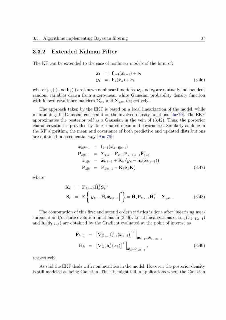
3.3. Algorithms implementing Bayesian filtering 37
3.3.2 Extended Kalman Filter
The KF can be extended to the case of nonlinear models of the form of:
xk = fk−1(xk−1) + νk
yk = hk(xk) + ek (3.46)
where fk−1(·) and hk(·) are known nonlinear functions. νk and ek are mutually independentrandom variables drawn from a zero-mean white Gaussian probability density functionwith known covariance matrices Σx,k and Σy,k, respectively.
The approach taken by the EKF is based on a local linearization of the model, whilemaintaining the Gaussian constraint on the involved density functions [Jaz70]. The EKFapproximates the posterior pdf as a Gaussian in the vein of (3.42). Thus, the posteriorcharacterization is provided by its estimated mean and covariances. Similarly as done inthe KF algorithm, the mean and covariance of both predictive and updated distributionsare obtained in a sequential way [And79]:
xk|k−1 = fk−1(xk−1|k−1)
Pk|k−1 = Σx,k + Fk−1Pk−1|k−1F>k−1
xk|k = xk|k−1 + Kk
(yk − hk(xk|k−1)
)Pk|k = Pk|k−1 −KkSkK
>k (3.47)
where
Kk = Pk|k−1H>k S−1
k
Sk = E∣∣∣yk − Hkxk|k−1
∣∣∣2 = HkPk|k−1H>k + Σy,k . (3.48)
The computation of this first and second order statistics is done after linearizing mea-surement and/or state evolution functions in (3.46). Local linearizations of fk−1(xk−1|k−1)and hk(xk|k−1) are obtained by the Gradient evaluated at the point of interest as
Fk−1 =[∇xk−1
f>k−1(xk−1)]> ∣∣∣xk−1=xk−1|k−1
Hk =[∇xkh>k (xk)
]> ∣∣∣xk=xk|k−1
, (3.49)
respectively.
As said the EKF deals with nonlinearities in the model. However, the posterior densityis still modeled as being Gaussian. Thus, it might fail in applications where the Gaussian
38 Chapter 3. Fundamentals of Bayesian Filtering
assumption is not valid or the nonlinearity is severe, which causes the true posterior todiffer from Gaussianity. In addition, the EKF requires an accurate initialization of statesand covariances in order to converge to the optimal solution, since the approximations in(3.49) are local.
3.3.3 The family of sigma-point Kalman filters
It is known that the EKF fails under severe nonlinearities. However, if the Gaussianassumption is still valid both for process and measurement noises we can seriously considerthe family of SPKFs to infer the states of our system. As shown in [Ito00], for an arbitrarynonlinearity, we can derive a recursive algorithm by equating the Bayesian formulae withrespect to the first and second moments of the distributions, that is, means and covariancesof the conditional densities involved. The Bayesian filtering problem is then cast into anumerical evaluation of the involved integrals in (3.8) and (3.9).
As stated in the previous Section, there are a number of alternatives to evaluate suchintegrals under the Gaussian assumption. Here we are interested in SPKFs, a familyof derivative-free algorithms which are based on a weighted sum of function values atspecified (i.e., deterministic) points within the domain of integration, as opposite to thestochastic sampling performed by particle filtering methods. A pseudocode description ofa generic SPKF is given in Algorithm 3.1, where it is easy to recognize the underlyingKF-like structure. This algorithm is valid for any SPKF–like algorithm, only differing onthe generation of sigma-points in step 1. Notice that weights are normalized such that∑
i ω(m)i =
∑i ω
(c)i = 1.
A further improvement of the standard SPKF scheme comes from the fact that, whenwe propagate the covariance matrix through a nonlinear function, the filter should preservethe properties of a covariance matrix, namely, its symmetry, and positive-definiteness. Inpractice, however, due to lack of arithmetic precision, numerical errors may lead to a lossof these properties. To circumvent this problem, a square-root filter can be considered topropagate the square root of the covariance matrix instead of the covariance itself. Evenmore, it avoids the inversion of the updated covariance matrix, entailing additional com-putational saving [Pot63]. The idea has been applied to the UKF [Van01] (although it doesnot guarantee positive definiteness of the covariance matrix) and, more successfully, to theSquare–Root Quadrature Kalman Filter (SQKF)[Ara08] and the Square–Root CubatureKalman Filter (SCKF) [Ara09].
3.3. Algorithms implementing Bayesian filtering 39
As an outcome of Algorithm 3.1 one obtains the two distributions in (3.8) and (3.9)as
p(xk|y1:k−1) ≈ N(xk|k−1,Σx,k|k−1
)(3.50)
p(xk|y1:k) ≈ N(xk|k,Σx,k|k
), (3.51)
respectively, which can be directly used to obtain an estimate of the states of interest.
Here we discuss the most popular algorithms falling in the SPKF category. As said,their sole difference is on the generation and weighting of sigma-points. At a glance:
UKF: It is based on the unscented transform (UT), whose sigma-points generation andweighting can be consulted6 in Algorithm 3.3. The UT uses 2nx + 1 points to op-timally characterize mean and covariance propagation of up to third order nonlin-earities, under the Gaussian assumption. The square–root unscented Kalman fil-ter (SRUKF) was first introduced in [Van01]. Intuitively, the role of parameter λ isto adjust the distance among the generated sigma–points and the mean. Therefore,if the dimension of the state–space increases, the distance also increases, forcing thetransform to take into account non-local effects. The parameters required for theUT to operate are: α is a positive scaling parameter which can be made arbitrarilysmall to minimize higher order effects (e.g. 10−3), and it determines the spread ofsigma-points around a mean value; κ is a secondary parameter typically set to 0;and β = 2 was seen to be optimal in the Gaussian case [Jul04].
CKF: Recently, the Cubature Kalman filter (CKF) and its square-root version (SR-CKF) were proposed in [Ara09]. The CKF is based on a spherical–radial cubaturerule [Str71] to generate and weight the sigma-points in Algorithm 3.1 and thus ap-proximate the integrals in (3.8) and (3.9). Specifically, the authors claim that athird–degree cubature rule is enough in many filtering problems over higher–degreerules. Moreover, a third-degree spherical-radial cubature rule is said to be an opti-mal approximation to the Bayesian filter when the Gaussian assumption holds. Thissetup yields a total of 2nx sigma–points, details found in Algorithm 3.4.
QKF: Another alternative for numerically solving the integrals in (3.8) and (3.9) is toresort to the Gauss–Hermite quadrature rules [Gol73]. Recently, this procedure wasused to develop the so-called Quadrature Kalman filter (QKF) [Ito00, Ara07] andthe corresponding square-root version (SRQKF) in [Ara08], exhibiting remarkableperformance results. A single parameter is required for the use of Gauss–Hermitequadrature rule, which is the number of sigma–points per dimension γ. The pseu-docode can be consulted in Algorithm 3.5. The square–root quadrature Kalman
6where 1i denotes the vector having a 1 at the i-th element and 0 otherwise.
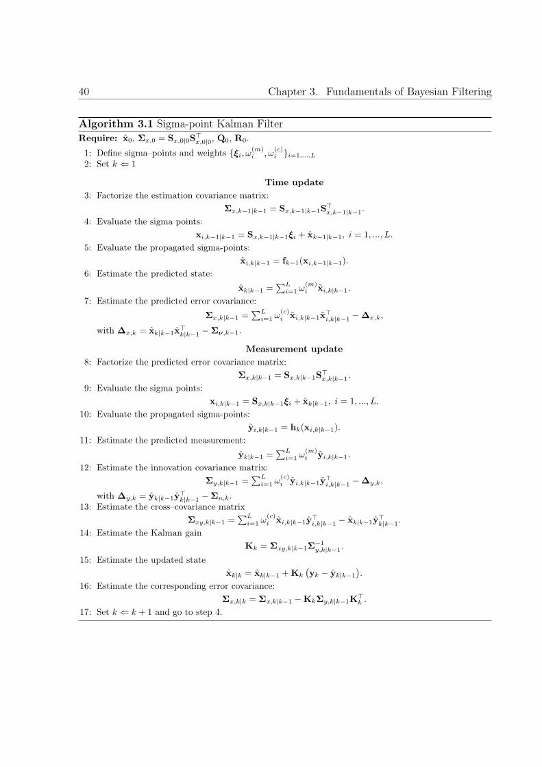
40 Chapter 3. Fundamentals of Bayesian Filtering
Algorithm 3.1 Sigma-point Kalman Filter
Require: x0, Σx,0 = Sx,0|0S>x,0|0, Q0, R0.
1: Define sigma–points and weights ξi, ω(m)i , ω
(c)i i=1,...,L
2: Set k ⇐ 1
Time update
3: Factorize the estimation covariance matrix:
Σx,k−1|k−1 = Sx,k−1|k−1S>x,k−1|k−1.
4: Evaluate the sigma points:
xi,k−1|k−1 = Sx,k−1|k−1ξi + xk−1|k−1, i = 1, ..., L.
5: Evaluate the propagated sigma-points:
xi,k|k−1 = fk−1(xi,k−1|k−1).
6: Estimate the predicted state:
xk|k−1 =∑Li=1 ω
(m)i xi,k|k−1.
7: Estimate the predicted error covariance:
Σx,k|k−1 =∑Li=1 ω
(c)i xi,k|k−1x
>i,k|k−1 −∆x,k,
with ∆x,k = xk|k−1x>k|k−1 −Σν,k−1.
Measurement update
8: Factorize the predicted error covariance matrix:
Σx,k|k−1 = Sx,k|k−1S>x,k|k−1.
9: Evaluate the sigma points:
xi,k|k−1 = Sx,k|k−1ξi + xk|k−1, i = 1, ..., L.
10: Evaluate the propagated sigma-points:
yi,k|k−1 = hk(xi,k|k−1).
11: Estimate the predicted measurement:
yk|k−1 =∑Li=1 ω
(m)i yi,k|k−1.
12: Estimate the innovation covariance matrix:
Σy,k|k−1 =∑Li=1 ω
(c)i yi,k|k−1y
>i,k|k−1 −∆y,k,
with ∆y,k = yk|k−1y>k|k−1 −Σn,k.
13: Estimate the cross–covariance matrix
Σxy,k|k−1 =∑Li=1 ω
(c)i xi,k|k−1y
>i,k|k−1 − xk|k−1y
>k|k−1.
14: Estimate the Kalman gain
Kk = Σxy,k|k−1Σ−1y,k|k−1.
15: Estimate the updated state
xk|k = xk|k−1 + Kk
(yk − yk|k−1
).
16: Estimate the corresponding error covariance:
Σx,k|k = Σx,k|k−1 −KkΣy,k|k−1K>k .
17: Set k ⇐ k + 1 and go to step 4.
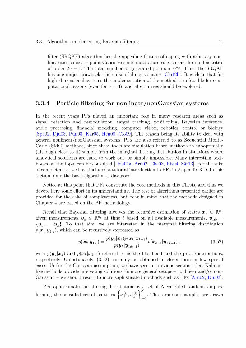
3.3. Algorithms implementing Bayesian filtering 41
filter (SRQKF) algorithm has the appealing feature of coping with arbitrary non-linearities since a γ-point Gauss–Hermite quadrature rule is exact for nonlinearitiesof order 2γ − 1. The total number of generated points is γnx . Thus, the SRQKFhas one major drawback: the curse of dimensionality [Clo12b]. It is clear that forhigh–dimensional systems the implementation of the method is unfeasible for com-putational reasons (even for γ = 3), and alternatives should be explored.
3.3.4 Particle filtering for nonlinear/nonGaussian systems
In the recent years PFs played an important role in many research areas such assignal detection and demodulation, target tracking, positioning, Bayesian inference,audio processing, financial modeling, computer vision, robotics, control or biology[Spe02, Dju03, Pun03, Kar05, Hen08, Clo09]. The reason being its ability to deal withgeneral nonlinear/nonGaussian systems. PFs are also referred to as Sequential Monte-Carlo (SMC) methods, since these tools are simulation-based methods to suboptimally(although close to it) sample from the marginal filtering distribution in situations whereanalytical solutions are hard to work out, or simply impossible. Many interesting text-books on the topic can be consulted [Dou01a, Aru02, Che03, Ris04, Sar13]. For the sakeof completeness, we have included a tutorial introduction to PFs in Appendix 3.D. In thissection, only the basic algorithm is discussed.
Notice at this point that PFs constitute the core methods in this Thesis, and thus wedevote here some effort in its understanding. The rest of algorithms presented earlier areprovided for the sake of completeness, but bear in mind that the methods designed inChapter 4 are based on the PF methodology.
Recall that Bayesian filtering involves the recursive estimation of states xk ∈ Rnx
given measurements yk ∈ Rny at time t based on all available measurements, y1:k =y1, . . . ,yk. To that aim, we are interested in the marginal filtering distributionp(xk|y1:k), which can be recursively expressed as
p(xk|y1:k) =p(yk|xk)p(xk|xk−1)
p(yk|y1:k−1)p(xk−1|y1:k−1) , (3.52)
with p(yk|xk) and p(xk|xk−1) referred to as the likelihood and the prior distributions,respectively. Unfortunately, (3.52) can only be obtained in closed-form in few specialcases. Under the Gaussian assumption, we have seen in previous sections that Kalman-like methods provide interesting solutions. In more general setups – nonlinear and/or non-Gaussian – we should resort to more sophisticated methods such as PFs [Aru02, Dju03].
PFs approximate the filtering distribution by a set of N weighted random samples,
forming the so-called set of particlesx
(i)k , w
(i)k
Ni=1
. These random samples are drawn
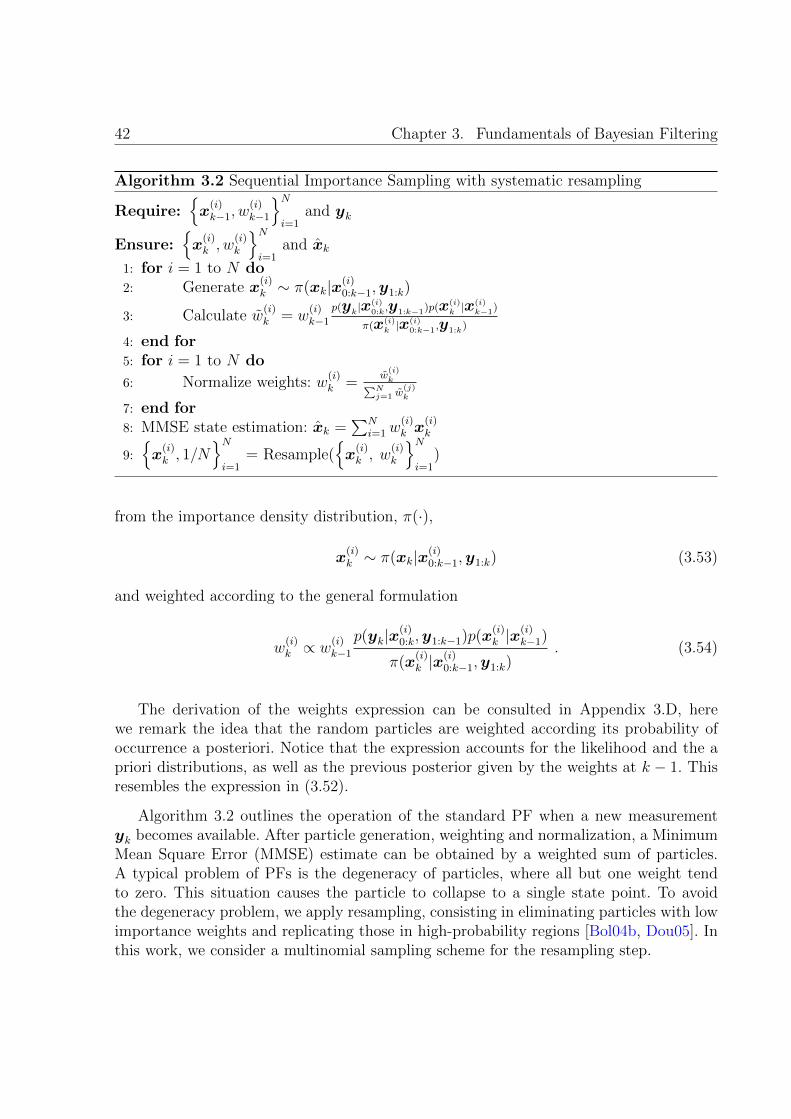
42 Chapter 3. Fundamentals of Bayesian Filtering
Algorithm 3.2 Sequential Importance Sampling with systematic resampling
Require:x
(i)k−1, w
(i)k−1
Ni=1
and yk
Ensure:x
(i)k , w
(i)k
Ni=1
and xk
1: for i = 1 to N do2: Generate x
(i)k ∼ π(xk|x(i)
0:k−1,y1:k)
3: Calculate w(i)k = w
(i)k−1
p(yk|x(i)0:k,y1:k−1)p(x(i)
k |x(i)k−1)
π(x(i)k |x
(i)0:k−1,y1:k)
4: end for5: for i = 1 to N do
6: Normalize weights: w(i)k =
w(i)k∑N
j=1 w(j)k
7: end for8: MMSE state estimation: xk =
∑Ni=1w
(i)k x
(i)k
9:
x
(i)k , 1/N
Ni=1
= Resample(x
(i)k , w
(i)k
Ni=1
)
from the importance density distribution, π(·),
x(i)k ∼ π(xk|x(i)
0:k−1,y1:k) (3.53)
and weighted according to the general formulation
w(i)k ∝ w
(i)k−1
p(yk|x(i)0:k,y1:k−1)p(x
(i)k |x
(i)k−1)
π(x(i)k |x
(i)0:k−1,y1:k)
. (3.54)
The derivation of the weights expression can be consulted in Appendix 3.D, herewe remark the idea that the random particles are weighted according its probability ofoccurrence a posteriori. Notice that the expression accounts for the likelihood and the apriori distributions, as well as the previous posterior given by the weights at k − 1. Thisresembles the expression in (3.52).
Algorithm 3.2 outlines the operation of the standard PF when a new measurementyk becomes available. After particle generation, weighting and normalization, a MinimumMean Square Error (MMSE) estimate can be obtained by a weighted sum of particles.A typical problem of PFs is the degeneracy of particles, where all but one weight tendto zero. This situation causes the particle to collapse to a single state point. To avoidthe degeneracy problem, we apply resampling, consisting in eliminating particles with lowimportance weights and replicating those in high-probability regions [Bol04b, Dou05]. Inthis work, we consider a multinomial sampling scheme for the resampling step.

3.4. Summary 43
There are many types of PFs based on the aforementioned concepts of Sequen-tial Importance Sampling (SIS), the most popular being Sampling Importance Resam-pling (SIR) filter [Gor93], Auxiliary SIR (ASIR) filter [Pit01, God01], Regularized par-ticle filter [Mus00], Local Linearization particle filter [Mer00], Gaussian particle fil-ter [Kot03a, Kot03b], Multiple Model particle filter [McG00], Rao-Blackwellized parti-cle filter [Sch05], Cost Reference particle filter [Mıg04], and multiple particle filtering[Bug07, Clo12a].
3.4 Summary
This chapter presented the basic ideas and tools in Bayesian filtering theory. At a glance,these tools become handy when inferring the evolution of signals that can be formulatedin state-space. The conceptual solution is not always analytically tractable, and thus weanalyzed the most popular approximation to the problem. We also discussed on theoreticallower bounds of accuracy and recursive formulae to compute these benchmark curves.

44 Chapter 3. Fundamentals of Bayesian Filtering
Appendix 3.A Useful equalities
The Chapman-Kolmogorov equation
Conditional densities can be manipulated in order to obtain more tractable expressionsby removing some variables. Denote some random variables as x1, x2 and x3. If we wantto remove x2 from the joint pdf f(x1, x2|x3), we integrate with respect to this variable,
f(x1|x3) =
∫ ∞−∞
f(x1|x2, x3)dx2 . (3.55)
On the other hand, if x2 has to be removed from f(x1|x2, x3), the Chapman-Kolmogorovequation [Pap01] is extensively used:
f(x1|x3) =
∫ ∞−∞
f(x1, x2|x3)f(x2|x3)dx2 . (3.56)
The Bayes’ rule
Bayes’ rule [Bay63] states that the probability density function of an event x conditionedto the event y can be expressed as
p(x|y) =p(y|x)p(x)
p(y), (3.57)
where the denominator can be computed using the Total probability theorem:
p(y) =
∫ ∞−∞
p(y|x)p(x)dx . (3.58)
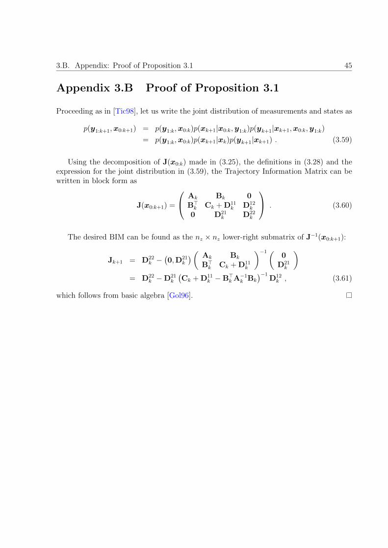
3.B. Appendix: Proof of Proposition 3.1 45
Appendix 3.B Proof of Proposition 3.1
Proceeding as in [Tic98], let us write the joint distribution of measurements and states as
p(y1:k+1,x0:k+1) = p(y1:k,x0:k)p(xk+1|x0:k,y1:k)p(yk+1|xk+1,x0:k,y1:k)
= p(y1:k,x0:k)p(xk+1|xk)p(yk+1|xk+1) . (3.59)
Using the decomposition of J(x0:k) made in (3.25), the definitions in (3.28) and theexpression for the joint distribution in (3.59), the Trajectory Information Matrix can bewritten in block form as
J(x0:k+1) =
Ak Bk 0B>k Ck + D11
k D12k
0 D21k D22
k
. (3.60)
The desired BIM can be found as the nz × nz lower-right submatrix of J−1(x0:k+1):
Jk+1 = D22k −
(0,D21
k
)( Ak Bk
B>k Ck + D11k
)−1(0
D21k
)= D22
k −D21k
(Ck + D11
k −B>k A−1k Bk
)−1D12k , (3.61)
which follows from basic algebra [Gol96].
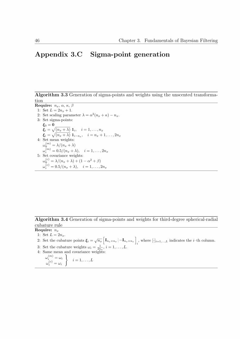
46 Chapter 3. Fundamentals of Bayesian Filtering
Appendix 3.C Sigma-point generation
Algorithm 3.3 Generation of sigma-points and weights using the unscented transforma-tionRequire: nx, α, κ, β
1: Set L = 2nx + 1.2: Set scaling parameter λ = α2(nx + κ)− nx.3: Set sigma-points:ξ0 = 0ξi =
√(nx + λ) 1i, i = 1, . . . , nx
ξi =√
(nx + λ) 1i−nx , i = nx + 1, . . . , 2nx4: Set mean weights:
ω(m)0 = λ/(nx + λ)
ω(m)i = 0.5/(nx + λ), i = 1, . . . , 2nx
5: Set covariance weights:
ω(c)0 = λ/(nx + λ) + (1− α2 + β)
ω(c)i = 0.5/(nx + λ), i = 1, . . . , 2nx
Algorithm 3.4 Generation of sigma-points and weights for third-degree spherical-radialcubature ruleRequire: nx
1: Set L = 2nx.
2: Set the cubature points ξi =√nx
[Inx×nx
−Inx×nx
]i, where [·]i=1,...,L indicates the i–th column.
3: Set the cubature weights ωi = 12nx
, i = 1, . . . , L.4: Same mean and covariance weights:
ω(m)i = ωi
ω(c)i = ωi
i = 1, . . . , L
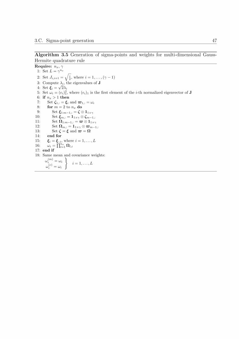
3.C. Sigma-point generation 47
Algorithm 3.5 Generation of sigma-points and weights for multi-dimensional Gauss-Hermite quadrature ruleRequire: nx, γ
1: Set L = γnx
2: Set Ji,i+1 =√
i2 , where i = 1, . . . , (γ − 1)
3: Compute λi, the eigenvalues of J4: Set ξi =
√2λi
5: Set ωi = (ei)21, where (ei)1 is the first element of the i-th normalized eigenvector of J
6: if nx > 1 then7: Set ζ1,: = ξi and $1,: = ωi8: for m = 2 to nx do9: Set ξ1:m−1,: = ζ ⊗ 11×γ
10: Set ξm,: = 11×γ ⊗ ζm−1,:11: Set Ω1:m−1,: = $ ⊗ 11×γ12: Set Ωm,: = 11×γ ⊗$m−1,:13: Set ζ = ξ and $ = Ω14: end for15: ξi = ξ:,i, where i = 1, . . . , L16: ωi =
∏nx
l=1 Ωl,i
17: end if18: Same mean and covariance weights:
ω(m)i = ωi
ω(c)i = ωi
i = 1, . . . , L

48 Chapter 3. Fundamentals of Bayesian Filtering
3.D. A Brief Introduction to Particle Filters 49
Appendix 3.D A Brief Introduction to Particle Fil-
ters
The basic ideas of SMC methods date back to [Ham54], but the widespread use in non-linear filtering theory is much more recent, the main reason being the high computationalcost required, which is only affordable in modern computing facilities. This appendixpresents a short overview of the fundamental concepts in particle filtering.
3.D.1 Monte-Carlo integration
The aim of PFs is to recursively estimate the posterior distribution p(x0:k|y1:k), themarginal filtering distribution p(xk|y1:k) and its associated expectations
I(gk) = E gk(x0:k)|y1:k =
∫gk(x0:k)p(x0:k|y1:k)dx0:k , (3.62)
with gk(·) a function of the state vector and the DSS model being as defined by equations(3.1) and (3.2) – or alternatively by (3.3) and (3.4).
PFs rely on the Monte-Carlo integration concept. Assume that we can simulate Ns
independent identically distributed (i.i.d.) random samples from p(x0:k|y1:k), this set is
denoted as x(i)0:k, i = 1, . . . , Ns. Then, the estimates of the distribution and its expecta-
tion are
ps(x0:k|y1:k) =1
Ns
Ns∑i=1
δ(x0:k − x(i)0:k)
Is(gk) =
∫gk(x0:k)ps(x0:k|y1:k)dx0:k =
1
Ns
Ns∑i=1
gk(x(i)0:k) , (3.63)
respectively. The estimate Is(gk) is unbiased and
P
lim
Ns→∞Is(gk) = I(gk)
= 1 , (3.64)
according to the law of large numbers [Cri02]. Moreover, if the variance of gk is finite, i.e.,
σ2gk
=
∫(gk(x0:k)− I(gk))
2p(x0:k|y1:k)dx0:k
=
∫g2k(x0:k)p(x0:k|y1:k)dx0:k − I2(gk) <∞ , (3.65)
50 Chapter 3. Fundamentals of Bayesian Filtering
then by the central limit theorem the estimation error converges in distribution, that is
limNs→∞
√Ns(Is(gk)− I(gk)) ∼ N
(0, σ2
gk
). (3.66)
Notice also that the rate of convergence is independent of the dimension of the integral, atleast in theory. However, it is well known that PFs suffer from the curse of dimensionality[Dau03]. The latter convergence results are the basis of the success of PFs, compared toother suboptimal algorithms that lack of theoretical foundations to ensure convergence tothe true posterior.
At this point one can wonder why such a method is named Monte-Carlo integration.Actually, it is a historically nomenclature since this method was first used to numericallysolve integrals [Pap01]. For example, if we want to integrate a function f(x), we can splitit into two components: one plays the role of the probability density function ϑ(x) whilethe other is the function g(x). Thus, the integral is obtained as
I =
∫f(x)dx =
∫g(x)ϑ(x)dx ≈ 1
Ns
Ns∑i=1
g(x(i)) , (3.67)
where Ns points are generated from ϑ(x).
3.D.2 Importance Sampling and Sequential Importance Sam-pling
Unfortunately, usually it is not possible to sample effectively from the posterior distribu-tion as required in (3.63), since it can be a complicated/unknown distribution. A classicalalternative is the Importance Sampling (IS) method [Gew89]. Imagine we can only gener-ate samples from a density π(x0:k|y1:k) which is similar to p(x0:k|y1:k), which means thatboth functions have the same support (in equation (3.79) and the corresponding text,further details will be given on this issue). We refer to π(x0:k|y1:k) as the importance orproposal density function. We can write equation (3.62) as
I(gk) =
∫gk(x0:k)p(x0:k|y1:k)dx0:k
=
∫gk(x0:k)
p(x0:k|y1:k)
π(x0:k|y1:k)π(x0:k|y1:k)dx0:k
=
∫gk(x0:k)w(x0:k)π(x0:k|y1:k)dx0:k , (3.68)
provided that w(x0:k) =p(x0:k|y1:k)
π(x0:k|y1:k)is upper bounded. Applying the Monte-Carlo inte-
gration method, we draw Ns independent samples from the importance density function,
3.D. A Brief Introduction to Particle Filters 51
x
(i)0:k
Nsi=1
, then an estimate of I(gk) is
Is(gk) =1
Ns
Ns∑i=1
gk(x(i)0:k)w(x
(i)0:k) , (3.69)
where
w(x(i)0:k) =
w(x(i)0:k)
Ns∑j=1
w(xj0:k)
(3.70)
are known as the normalized importance weights, and
w(x(i)0:k) =
p(x0:k|y1:k)
π(x(i)0:k|y1:k)
(3.71)
are the unnormalized importance weights, which are normalized in (3.70) to obtain aproper probability density function.
The IS method has one main drawback which makes it inadequate for recursive fil-tering purposes: to estimate p(x0:k|y1:k) one needs to have all data y1:k available. Then,when new data is available, one has to compute the importance weights over the entirestate trajectory. Thus, the computational complexity increases with time. Instead, weare interested in an algorithm that is able to include new data in the estimation processwithout recomputing weights from the scratch.
In an attempt to obtain a sequential algorithm relying on IS method, the SIS algo-rithm is obtained. It is a Monte-Carlo method that forms the basis of most SMC-basedfilters, being the natural recursive version of IS to approach the optimal Bayesian solution.Recalling from the IS method, we have that the posterior distribution is characterized by
the Ns generated points and its associated normalized weights,x
(i)0:k, w
(i)0:k
Nsi=1
, as
p(x0:k|y1:k) ≈Ns∑i=1
w(i)k δ(x0:k − x(i)
0:k)
w(i)k ∝ p(x
(i)0:k|y1:k)
π(x(i)0:k|y1:k)
. (3.72)
Under the assumption that we have a discrete approximation of p(x0:k−1|y1:k−1), theaim of SIS is to obtain a set of particles that characterize the distribution at k when new
52 Chapter 3. Fundamentals of Bayesian Filtering
measurements are received, yk. If we choose the importance function to factorize as
π(x0:k|y1:k) = π(xk|x0:k−1,y1:k)π(x0:k−1|y1:k−1)
= π(x0)k∏t=1
π(xt|y0:t−1,y1:t) , (3.73)
then the generation of samples can be done by augmenting the existing samplesx
(i)0:k−1 ∼ π(x0:k−1|y1:k−1)
Nsi=1
(3.74)
with the new state being x
(i)k ∼ π(xk|x0:k−1,y1:k)
Nsi=1
. (3.75)
The associated weights are computed from the following posterior recursion:
p(x0:k|y1:k) =p(yk|x0:k,y1:k−1)p(x0:k|y1:k−1)
p(yk|y1:k−1)
=p(yk|x0:k,y1:k−1)p(xk|x0:k−1,y1:k−1)p(x0:k−1|y1:k−1)
p(yk|y1:k−1)
=p(yk|xk)p(xk|xk−1)
p(yk|y1:k−1)p(x0:k−1|y1:k−1)
∝ p(yk|xk)p(xk|xk−1)p(x0:k−1|y1:k−1) , (3.76)
which only depends on the posterior at time k − 1 and the likelihood and the prior attime k. Given that p(x0) , p(x0|y0), where y0 is the set of no measurements, we canassume that the required density at time k − 1 is available in the sequential approach.Substitution of (3.73) and (4.15) in (3.72) yields to the weight update equation,
w(i)k ∝ w
(i)k−1
p(yk|x(i)k )p(x
(i)k |x
(i)k−1)
π(x(i)k |x
(i)0:k−1,y1:k)
. (3.77)
Now the recursion is closed and we are able to find an approximation of the filteringdistribution given by
p(xk|y1:k) =Ns∑i=1
w(i)k δ(xk − x
(i)k ) , (3.78)
being δ(·) the Kronecker’s delta function. This approximation converges a.s. to the trueposterior7 as Ns → ∞ under weak assumptions, according to the strong law of large
7Notice that a.s. convergence is equivalent to convergence w.p.1. Then, the convergence of the SISestimate of the filtering distribution is expressed as
P p(xk|y1:k)→ p(xk|y1:k) = 1 as Ns →∞ .
3.D. A Brief Introduction to Particle Filters 53
numbers [Dou98, Cri02]. These assumptions hold if the support of the chosen importancedensity (π) include the support of the filtering distribution (p), i.e.,
π = xk ∈ Rnx| π(xk|y1:k) > 0p = xk ∈ Rnx| p(xk|y1:k) > 0
and p ⊆ π . (3.79)
Thus, for the convergence results to hold we have to ensure that the importancefunction has the same support as the true posterior, meaning that the set closure of theset of arguments of these functions for which the value is not zero is the same.
From the new set of sample points, one can compute a number of statistics. As con-ceptually presented in (3.11) and (3.12), the MMSE and MAP estimators can be obtainedas
xMMSEk =
Ns∑i=1
w(i)k x
(i)k (3.80)
xMAPk = arg max
x(i)k
w
(i)k
, (3.81)
respectively. The covariance (or uncertainty region) of an estimate xk can be calculatedas
Σx =Ns∑i=1
w(i)k
(x
(i)k − xk
)(x
(i)k − xk
)>. (3.82)
A pseudocode description of the SIS algorithm is shown in Algorithm 3.6. Noticethat SIS is an algorithm that approximates the posterior by sequentially updating themeasurement vector and propagating the importance weights. Basically, to sum up, itinvolves the approximation of the posterior by a set of Ns random samples taken from animportance density function, x
(i)k ∼ π(xk|x(i)
0:k−1,y1:k), with associated importance weights
w(i)k . The choice of π(·) is a critical issue in the design of any PF, which still remains as an
open topic for statisticians [Dou00] and is usually an application-dependent issue. For a
set of generated particles,x
(i)k , w
(i)k
Nsi=1
, the approximation of the filtering distribution
as given by PFs is obtained via equation (3.78).
3.D.3 Resampling
Everything has its payback, and PFs are not the exception. The main drawback of theSIS algorithm is that it suffers from the so-called degeneracy phenomenon, which states

54 Chapter 3. Fundamentals of Bayesian Filtering
Algorithm 3.6 Sequential Importance Sampling (SIS) algorithm
Require:x
(i)k−1, w
(i)k−1
Nsi=1
and yk
Ensure:x
(i)k , w
(i)k
Nsi=1
1: for i = 1 to Ns do2: Generate x
(i)k ∼ π(xk|x(i)
k−1,y1:k)
3: Calculate w(i)k = w
(i)k−1
p(yk|x(i)k )p(x(i)
k |x(i)k−1)
π(x(i)k |x
(i)0:k−1,y1:k)
4: end for5: for i = 1 to Ns do
6: Normalize weights: w(i)k =
w(i)k∑Ns
j=1 wjk
7: end for
that the variance of importance weights can only increase over time [Dou00]. In otherwords, after a certain number of sequential steps, one finds that the value of one of thenormalized weights tends to 1 while the rest tend to 0. The problem then is to keepparticle trajectories with significant weights and remove those which hardly contribute tothe estimation of the filtering distribution. The solution was proposed in [Rub88] and isknown as resampling : discarding samples with low importance weights and keep/multiplythose with high importance weights. Resampling was proposed for SIS in a number ofworks [Gor93, Liu95, Ber97].
A measure of the degeneracy is the effective sample size Neff , introduced in [Kon94],which is estimated as
Neff =1∑Ns
i=1
(w
(i)k
)2 (3.83)
where 1 ≤ Neff ≤ Ns and values close to the lower bound indicate high degeneracy. Thecommon approach is to specify a threshold such that, when the effective sample size isbelow, indicates the algorithm to apply resampling (see Algorithm 3.7). Although highlydependent on the chosen threshold, this approach is the most used in the literature. In[Ber99] a suggested threshold is Nth = 2
3Ns.
The process of resampling particles can be implemented in several ways. Commonschemes include multinomial resampling [Gor93], residual resampling [Liu98] and strat-ified/systematic resampling [Kit96, Cri01]. It is out of the scope of the dissertation thestudy of novel resampling strategies, in the sequel a multinomial resampling is consideredwhich is one of the easiest to implement.
Although it solves the degeneracy phenomenon, resampling can result in a sampleimpoverishment, that is particles with high weights are selected many times. Notice that
3.D. A Brief Introduction to Particle Filters 55
Algorithm 3.7 Generic Particle Filtering with Resampling
Require:x
(i)k−1, w
(i)k−1
Nsi=1
and yk
Ensure:x
(i)k , w
(i)k
Nsi=1
1:
[x
(i)k , w
(i)k
Nsi=1
]= SIS(
x
(i)k−1, w
(i)k−1
Nsi=1
, yk)
2: Calculate Neff
3: if Neff < Nth then
4: Resample Particles:
[x
(i)k , w
(i)k
Nsi=1
]= Resample(
x
(i)k , w
(i)k
Nsi=1
)
5: end if
this loss of diversity is severe when process noise is small [Gor93, Hig95]. Thus, convergenceresults of the algorithm should be re-established [Ber97]. Another undesired aspect ofresampling is that it constitutes the bottleneck in any parallel implementation of PFs[Bol05], since all particles must be combined in this process.
Nevertheless, resampling is a key step in the design of a PF since degeneracy jeopar-dizes posterior estimates in a way that cannot be tolerated. Many work has been directedin the design of efficient resampling strategies and architectures [Bol04a].
3.D.4 Selection of the importance density
One of the key points of a PF algorithm is the choice of a good importance density function,π(xk|x(i)
0:k−1,y1:k). Actually, a bad choice can lead the algorithm to a poor characterizationin (3.78) and, thus, to a bad performance. Some common alternatives might be found inthe literature:
The optimal choice
Since the aim of a PF is to characterize the filtering distribution, it is quite intuitive tosay that this distribution is the best choice for particle generation. Indeed, the optimaldistribution is the target distribution that we wish to estimate:
π(xk|x(i)0:k−1,y1:k) = p(xk|x(i)
0:k−1,y1:k) , (3.84)
which is optimal in the sense that it minimizes the variance of importance weights con-ditional upon the trajectory and the observations [Dou00]. The use of such an optimal
56 Chapter 3. Fundamentals of Bayesian Filtering
importance density reduces the degeneracy effect discussed previously. In this case, thecalculation of weights reduces to:
w(i)k ∝ w
(i)k−1p(yk|x
(i)k−1) , (3.85)
which does not depend on the current particle value x(i)k , facilitating parallelization of the
PF [Bol04a].
Thus, in order to use the optimal importance density, one has to i) be able to draw
samples from p(xk|x(i)0:k−1,y1:k) and to ii) evaluate
p(yk|xk−1) =
∫p(yk|xk)p(xk|xk−1)dxk . (3.86)
Few special cases can be found that allow the generation/evaluation from these distribu-tions. One case is when the states xk are finite, as in [Dou01b]. Another case is when theDSS model is Gaussian with linear measurements [Dou00, Ris04]. Unfortunately, thesetwo requirements may not hold in general and one has to resort to suboptimal choices.
Suboptimal choices
Since the only condition imposed on π(xk|x(i)0:k−1,y1:k) is to fulfill (3.73), the amount of
possible suboptimal importance densities seems huge8. Indeed, a general methodology forselecting an importance density is still missing, being several alternatives proposed in theliterature. Actually, in most of the cases this choice highly depends on the applicationitself and has to be carefully designed.
The simplest approach, and the most popular, is to consider the transitional prior asthe importance function. In this case, weights are proportional to the likelihood function:
π(xk|x(i)0:k−1,y1:k) = p(xk|x(i)
k−1)
w(i)k ∝ w
(i)k−1p(yk|x
(i)k ) . (3.87)
The popularity of the transitional prior choice is due to its simple implementationand the lack of computationally intensive calculations. Note that in the Gaussian case,generation in (3.87) reduces to sample from a Gaussian distribution. Nevertheless, thischoice was shown to be inefficient as it requires a large number of samples to effectivelycharacterize the posterior distribution [Ris04]. The main reason is that, since measure-ments are not taken into consideration when generating particles, the algorithm is likelyto exhibit a high degeneracy.
8Keeping in mind that the importance density has to share the same support as the target distribution,in order to claim convergence [Cri02].

3.D. A Brief Introduction to Particle Filters 57
More sophisticated, though also suboptimal, alternatives aim at approximating the op-timal importance density in (3.84). Although they require a higher computational burden,their performance is typically better than the one provided by the transitional prior. Someof the strategies reported in the literature include local model linearization [Dou00], Gaus-sian approximations [Kot03a] or the use of the unscented transform [Mer00]. In Section3.3.4 of this dissertation, we consider another importance density function. The methodwas originally proposed in [Cev07] for an acoustic multitarget tracking problem. Basicallyit is based on a Gaussian approximation of the optimal distribution.

58 Chapter 3. Fundamentals of Bayesian Filtering

4Sequential estimation of neuralactivity from voltage traces in
single-neuron models
THE membrane potential, obtained from intracellular recordings, is one of the mostvaluable signals of neurons’ activity. Most of the neuron models have been derived
from fine measurements and allow the progress of “in silico” experiments. However, otherinteresting quantities informing about the neuron’s intrinsic activity or synaptic connec-tions [Piw04, Bed11] are either costly to obtain (channel blocking and clamping techniques[Hod52, Bre12]) or impossible to measure explicitly with today’s techniques. Thus, estima-tion methods can be very useful, mostly those that can be applied to obtain time evolutionon-line; that is, avoiding the need of repetitions that could be contaminated by neuronalvariability. In this chapter, as a first step, we concentrate on methods to extract intrinsicactivity of ionic channels, namely the probabilities of opening and closing channels. Tothis purpose, we consider a neuron model and, using a PF algorithm with optimal impor-tance density, we recover both the membrane potential and the activity of the potassiumchannel with the minimum attainable error. Moreover, we design an enhanced algorithmthat can cope with model uncertainties and thus relaxing the assumption of perfect modelknowledge of the former algorithm.
59
60 Chapter 4. Sequential estimation of neural activity
In the open literature similar solutions could be found. [Kob11] deals with a similarinference problem, under correct model assumptions for the ionic channels [Pos08], andsolve the filtering problem by a Kalman filter. The authors assume synaptic inputs aswhite noise and estimate the mean and variances of the process.
Another similar setup is treated in [Pan12], where a PF is used to filter voltage andsynaptic conductances. In this case, the voltage observations are assumed subthreshold,as opposite to our approach in this Thesis. A similar solution, this time based on theGaussian mixture Kalman filtering, was proposed in [Lan13]. More recently, the same au-thors proposed in [Lan14] a Kalman-like solution to estimate voltage and gating variables,as well as the maximal conductances of the ionic channels (thus implicitly assuming thelatter as time-varying). Our approach is similar in essence, although we go further in themethod and present a solution that can cope with the estimation of any time-varyingsignal in the system (gathered in the state vector) and those deterministic parametersthat describe the model (gathered in an unknown parameter vector).
In [Rud03, Bed11], it is shown how to extract synaptic conductances from noisy voltagetraces. The work considers subthreshold activity. This approach might introduce errors insituations where spiking is present or when there is sub-threshold ionic activity [Gui06].The approach we follow in this Thesis is to work in the spike regime, without the sub-threshold assumption [Clo13b, Clo13a].
The remainder of the chapter is organized as follows. The problem is stated in discretestate-space in Section 4.1, for which we focused in the model named after Morris and Lecarintroduced in Section 2.3.1. The main causes of model inaccuracies are enumerated inSection 4.2, as well as hints to account for them in the method. We present a PF solutionfor the filtering problem under perfect model knowledge in Section 4.3 and design anenhanced algorithm that can estimate the parameters of the model in Section 4.4. Section4.5 discusses computer simulations, with comparison to the theoretical estimation boundsderived in Appendix 4.A, and Section 4.6 wraps up the main conclusions of the study.
4.1 Problem statement
As introduced earlier in Chapter 2, the problem investigated in this Thesis considersrecordings of noisy voltage traces to infer the hidden gating variables of the neuron model,as well as filtered voltage estimates. Data is recorded at discrete time-instants k at asampling frequency fs = 1/Ts. The problem can thus be posed in the form of a discrete-time, state-space model. The observations are
yk ∼ N (vk, σ2y,k) , (4.1)

4.1. Problem statement 61
with σ2y,k modeling the noise variance due to the sensor or the instrumentation inaccuracies
when performing the experiment. To provide comparable results, we define the signal-to-noise ratio (SNR) as SNR = Ps/Pn, with Ps being the average signal power and Pn = σ2
y,k
the noise power.
On the other hand, we have models for the evolution of the voltage-traces and thehidden variables of a neuron. For instance, the Morris-Lecar model presented in Section2.3.1. The unknown state vector in this case is
xk =
(vknk
). (4.2)
Notice that the Morris-Lecar neuron model is defined by a system of continuous-time,ODEs. In general, all the mathematical models for neurons are of this type. However, weare interested in expressing the model in the form of a discrete state-space,
xk = fk(xk−1) + νk , (4.3)
where νk ∼ N (0,Σx,k) is the process noise which includes the model inaccuracies. Thecovariance matrix Σx,k is used to quantify our confidence in the model that maps fk :vk−1, nk−1 7→ vk, nk. In general, obtaining a closed-form analytical expression forfk without approximations is not possible. An alternative option are numerical methods,which aim at solving the differential equation at discrete instants. One simple, yet popular,method to approximate x = f(x) is the Euler method (a finite difference approximation)that is based on the approximation
x.=dx
dt≈ ∆x
∆t= f(x) (4.4)
where ∆t = Ts is the sampling period and thus,
∆x
∆t=x(t+ Ts)− x(t)
Ts
= f(x(t)) (4.5)
or equivalently in discrete notation
x ≈ xk − xk−1
Ts
= f(xk−1) , (4.6)
from which it follows that
xk = xk−1 + Tsf(xk−1) , (4.7)
which is of the Markovian type in (3.1).

62 Chapter 4. Sequential estimation of neural activity
If we focus on the Morris-Lecar model, the resulting discrete version of the ODEsystem in (2.8)-(2.9) is:
vk = vk−1 −Ts
Cm
(gL(vk−1 − EL)
+ gCam∞(vk−1)(vk−1 − ECa) + gKnk−1(vk−1 − EK)− Iapp
)(4.8)
nk = nk−1 + Tsφn∞(vk−1)− nk−1
τn(vk−1), (4.9)
with m∞(vk), n∞(vk), and τn(vk) defined as in (2.13)-(2.15). Then, (4.8) and (4.9) can beinterpreted as xk = fk(xk−1).
The goal is to express the inference problem in state-space formulation and apply thetools learned in Chapter 3. The final ingredient to do so is to introduce the so-calledprocess noise in the state equation
xk = fk(xk−1) +
(νv,kνn,k
), (4.10)
where the noise terms νv,k and νn,k are jointly Gaussian with covariance matrix Σx,k.Further details of this matrix are discussed in Section 4.2.
4.2 Model inaccuracies
The proposed estimation method highly relies on the fact that the neuron model is known.This is true to some extend, but most of the parameters in the model discussed in Section2.3.1 are to be estimated beforehand. Therefore, the robustness of the method to possibleinaccuracies should be assessed. In this section, we point out possible causes of missmod-eling. In next section, computer simulations are used to characterize the performance ofthe method under these impairments.
In the single-neuron model considered, three major sources of inaccuracies can beidentified:
1. The applied current Iapp can be itself noisy, with a variance depending on the qualityof the instrumentation used and the experiment itself. We model the actual appliedcurrent as the random variable
Iapp = Io + νI,k , νI,k ∼ N (0, σ2I ) , (4.11)
where Io is the nominal current applied and σ2I the variance around this value.
Plugging (4.11) into (4.8) we obtain that the contribution of Iapp to the noise term
is TsCmνI,k ∼ N (0, (Ts/Cm)2σ2
I ).
4.3. Sequential estimation of voltage traces and gating variables by particle filtering 63
2. The conductance of the leakage term has to be estimated beforehand. In general,this term is considered constant although it gathers relatively distinct phenomenathat can potentially be time-varying. The maximal conductance of the leakage termis therefore inaccurate and modeled as
gL = goL + νg,k , νg,k ∼ N (0, σ2g) , (4.12)
where goL is the nominal, estimated conductance and σ2g the variance of this estimate.
Similarly, inserting (4.12) into (4.8) we see that the contribution of gL to the noise
term is TsCmνg,k ∼ N (0, (Ts/Cm)2(vk−1 − EL)σ2
g).
3. The parameters in m∞(vk), n∞(vk), and τn(vk) are to be estimated. In general, theseparameters are properly obtained by standard methods [Izh06]. However, as they areestimates, a residual error typically remains. To account for these inaccuracies, weconsider that the equation governing the evolution of gating variables is corruptedby a zero-mean additive white Gaussian process with variance σ2
n.
At the end of the day, we came up with a way of constructing the model covariancematrix, as the contribution of the aforementioned inaccuracies. In a practical setup, inorder to compute the noise variance due to leakage, we need to use the approximationvk−1 ≈ vk−1, where vk−1 is computed by the filter. We construct the covariance matrix ofthe model as
Σx,k =
(σ2v 0
0 σ2n
), (4.13)
where we used that the overall noise in the voltage model is TsCm
(νI,k − νg,k) ∼ N (0, σ2v)
and
σ2v =
(Ts
Cm
)2 (σ2I + (vk−1 − EL)2σ2
g
)(4.14)
could be an estimate of σ2v , provided accurate knowledge of σ2
I and σ2g . Otherwise, the
covariance matrix of the process has to be estimated by other means, as the ones presentedin this Chapter for mixed state-parameter estimation in nonlinear filtering problems.
4.3 Sequential estimation of voltage traces and gat-
ing variables by particle filtering
Bayesian filtering involves the recursive estimation of states xk ∈ Rnx given measurementsyk ∈ R at time t based on all available measurements, y1:k = y1, . . . , yk. To that aim, we
64 Chapter 4. Sequential estimation of neural activity
are interested in the filtering distribution p(xk|y1:k), which can be recursively expressedas
p(xk|y1:k) =p(yk|xk)p(xk|xk−1)
p(yk|y1:k−1)p(xk−1|y1:k−1) , (4.15)
with p(yk|xk) and p(xk|xk−1) referred to as the likelihood and the prior distributions,respectively. Unfortunately, (4.15) can only be obtained in closed-form in some specialcases and in more general setups we should resort to more sophisticated methods. In thispaper we consider PF to overcome the nonlinearity of the model [Dju03].
As explained in Section 3.3.4, PFs approximate the filtering distribution by a set of
N weighted random samples, forming the random measurex
(i)k , w
(i)k
Ni=1
. These random
samples are drawn from the importance density distribution, π(·),
x(i)k ∼ π(xk|x(i)
0:k−1, y1:k) (4.16)
and weighted according to the general formulation
w(i)k ∝ w
(i)k−1
p(yk|x(i)0:k, y1:k−1)p(x
(i)k |x
(i)k−1)
π(x(i)k |x
(i)0:k−1, y1:k)
. (4.17)
The importance density from which particles are drawn is a key issue in designingefficient PFs. It is well-known that the optimal importance density is π(xk|x(i)
0:k−1, y1:k) =
p(xk|x(i)k−1, yk), in the sense that it minimizes the variance of importance weights. Weights
are computed using (4.17) as w(i)k ∝ w
(i)k−1p(yk|x
(i)k−1). This choice requires the ability to
draw from p(xk|x(i)k−1, yk) and to evaluate p(yk|x(i)
k−1). In general, the two requirementscannot be met and one needs to resort to suboptimal choices. However, we are able to usethe optimal importance density since the state-space model assumed here is Gaussian, withnonlinear process equations but related linearly to observations [Dou00]. The equationsare:
p(xk|x(i)k−1, yk) = N (µ
(i)π,k,Σπ,k) (4.18)
with
µ(i)π,k = Σπ,k
(Σ−1x,kfk(x
(i)k−1) +
ykσ2y,k
)(4.19)
Σπ,k =(Σ−1x,k + σ−2
y,kI)−1
, (4.20)
and the importance weights can be updated using
p(yk|x(i)k−1) = N (hfk(x
(i)k−1),hΣx,kh
> + σ2y,k) , (4.21)
4.3. Sequential estimation of voltage traces and gating variables by particle filtering 65
with h = (1, 0). The PF provides a discrete approximation of the filtering distribution of
the form p(xk|y1:k) ≈∑N
i=1 w(i)k δ(xk − x
(i)k ), which gather all information from xk that
the measurements up to time t provide. This was discussed when introducing (3.78). Forinstance, the minimum mean square error estimator can be obtained as
xk =N∑i=1
w(i)k x
(i)k , (4.22)
where xk = (vk, nk)>. Recall that the method discussed in this section could be eas-
ily adapted to other neuron models simply substituting by the corresponding transitionfunction fk and constructing the state vector xk conveniently.
As a final step, PFs incorporate a resampling strategy to avoid collapse of particlesinto a single state point. As introduced earlier in Section 3.3.4, resampling consists ineliminating particles with low importance weights and replicating those in high-probabilityregions [Dou05]. The overall algorithm can be consulted in Algorithm 4.1 at instance k.Notice that this version of the algorithm requires knowledge of noise statistics and all themodel parameters
Θ = (gL, EL, gCa, ECa, gK, EK, φ, V1, V2, V3, V4)> . (4.23)
Algorithm 4.1 Particle filtering with optimal importance density
Require: Σx,k, σ2y,k, Θ,
x
(i)k−1, w
(i)k−1
Ni=1
and yk
Ensure:x
(i)k , w
(i)k
Ni=1
and xk
1: Calculate Σπ,k =(Σ−1x,k + σ−2
y,kI)−1
2: for i = 1 to N do3: Calculate µ
(i)π,k = Σπ,k
(Σ−1x,kfk(x
(i)k−1) + yk
σ2y,k
)4: Generate x
(i)k ∼ N (µ
(i)π,k,Σπ,k)
5: Calculate w(i)k = w
(i)k−1
p(yk|x(i)0:k,y1:k−1)p(x(i)
k |x(i)k−1)
N (µ(i)π,k,Σπ,k)
6: end for7: for i = 1 to N do
8: Normalize weights: w(i)k =
w(i)k∑N
j=1 w(j)k
9: end for10: MMSE state estimation: xk =
∑Ni=1w
(i)k x
(i)k
11:
x
(i)k , 1/N
Ni=1
= Resample(x
(i)k , w
(i)k
Ni=1
)
66 Chapter 4. Sequential estimation of neural activity
4.4 Joint estimation of states and model parameters
by particle filtering
In practice the parameters in (4.23) might not be known. It is reasonable to assume thatΘ, or a subset of these parameters θ ⊆ Θ, are unknown and need to be estimated at thesame time the filtering method in Algorithm 4.1 is executed. Therefore, the ultimate goalin this case is to estimate jointly the time evolving states and the unknown parametersof the model, x and θ respectively.
We follow the approach in [Sar13] to present one of the possible methodologies toenhance the PF presented in Algorithm 4.1 with parameter estimation capabilities. Jointestimation of states and parameters is a longstanding problem in Bayesian filtering, andspecially hard to handle in the context of PFs. Refer to [And04, And05, Poy11] and thereferences for a complete survey.
Following the Bayesian philosophy adopted in this Thesis, the problem fundamentallyreduces to assigning an a priori distribution for the unknown parameter θ ∈ Rnθ andextending the state-space model in (3.3)-(3.4) with
θ ∼ p(θ) (4.24)
xk ∼ p(xk|xk−1,θ) for k ≥ 1 (4.25)
yk ∼ p(yk|xk,θ) for k ≥ 1 (4.26)
and initial state distribution x0 ∼ p(x0|θ). Applying Bayes rule, the full posterior distri-bution can be expressed as
p(x0:T ,θ|y1:T ) =p(y1:T |x0:T ,θ)p(x0:T |θ)p(θ)
p(y1:T )(4.27)
with
p(y1:T |x0:T ,θ) =T∏k=1
p(yk|xk,θ) (4.28)
p(x0:T |θ) = p(x0|θ)T∏k=1
p(xk|xk−1,θ) . (4.29)
Notice here that we are dealing with a finite horizon of observations T . Then, from aBayesian perspective, the estimation of θ is equivalent to obtaining its marginal posteriordistribution
p(θ|y1:T ) =
∫p(x0:T ,θ|y1:T )dx0:T ; (4.30)
4.4. Joint estimation of states and model parameters by particle filtering 67
however, this is in general extremely hard to compute analytically and one needs to findworkarounds. Evaluation of the full posterior turns to be not only computationally pro-hibitive, but useless if states cannot be marginalized out analytically. Alternative methodsresort on the factorization of the parameter marginal distribution as
p(θ|y1:T ) = p(y1:T |θ)p(θ) (4.31)
and how Bayesian filters can be transformed to provide characterizations of the marginallikelihood distribution p(y1:T |θ) and related quantities. The marginal likelihood distribu-tion can be recursively factorized in terms of the predictive distributions of the observa-tions:
p(y1:T |θ) =T∏k=1
p(yk|y1:k−1,θ) , (4.32)
with
p(yk|y1:k−1,θ) = Exk|y1:k−1,θ
p(yk|xk,θ)
(4.33)
=
∫p(yk|xk,θ)p(xk|y1:k−1,θ)dxk (4.34)
obtained straightforwardly as a byproduct of any of the Bayesian filtering methods dis-cussed earlier in Section 3.3.
A useful transformation of the marginal likelihood is the so-called energy function,which is sometimes more convenient when implementing the solution. The energy functionis defined as
ϕT (θ) = − ln p(y1:T |θ) (4.35)
= − ln p(y1:T |θ)− ln p(θ) (4.36)
or, equivalently, p(y1:T |θ) ∝ exp(−ϕT (θ)). The energy function can then be recursivelycomputed as a function of the predictive distribution
ϕ0(θ) = − ln p(θ) (4.37)
ϕk(θ) = ϕk−1(θ)− ln p(yk|y1:k−1,θ) for k ≥ 1 . (4.38)
Then, the basic problem is to obtain an estimate of the predictive distributionp(yk|y1:k−1,θ) from the PF we have designed in Section 4.3 and use it in conjunctionwith p(θ) to infer the marginal distribution p(θ|y1:T ) of interest. This latter step canbe performed in several ways, from which we choose to use the Markov-Chain Monte-Carlo (MCMC) methodology to continue with a fully Bayesian solution. Besides, it isknown to be the solution that provides best results when used in a PF. Next, we de-tail how ϕk(θ) can be obtained from a PF algorithm, present the MCMC method forparameter estimation, and finally we sketch the overall algorithm.
68 Chapter 4. Sequential estimation of neural activity
Computing the energy function from particle filters:
The modification needed is very small. Actually, it is non-invasive in the sense that thealgorithm remains the same and the energy function can be computed adding some extraequations. Recall that the predictive distribution is
p(yk|y1:k−1,θ) =
∫p(yk|xk,θ)p(xk|y1:k−1,θ) (4.39)
and that the PF provides characterizations of the two distributions in the integral. Then,one can get an approximation by
p(yk|y1:k−1,θ) ≈ p(yk|y1:k−1,θ) (4.40)
=N∑i=1
w(i)k−1ζ
(i)k (4.41)
with w(i)k−1 as in the original algorithm and
ζ(i)k =
p(yk|x(i)k ,θ)p(x
(i)k |x
(i)k−1,θ)
π(x(i)k |x
(i)0:k−1,y1:k,θ)
. (4.42)
Then, it is straightforward to identify the energy function approximation as
ϕT (θ) = − ln p(θ)− ln p(y1:T |θ) (4.43)
= − ln p(θ)− lnT∏k=1
p(yk|y1:k−1,θ) (4.44)
= − ln p(θ)−T∑k=1
ln p(yk|y1:k−1,θ) (4.45)
≈ − ln p(θ)−T∑k=1
ln p(yk|y1:k−1,θ) (4.46)
= − ln p(θ)−T∑k=1
lnN∑i=1
w(i)k−1ζ
(i)k = ϕT (θ) , (4.47)
which can be computed recursively in the PF algorithm.
The Particle Markov-Chain Monte-Carlo algorithm:
Once an approximation of the energy function is available, we can apply MCMC to inferthe marginal distribution of the parameters. MCMC methods constitute a general method-ology to generate samples recursively from a given distribution by randomly simulating
4.4. Joint estimation of states and model parameters by particle filtering 69
from a Markov chain [Gil96, Ber97, Liu08, Bro11]. There are many algorithms implement-ing the MCMC concept, being one of the most popular the Metropolis-Hastings (MH)algorithm. At the j-th iteration, the MH algorithm samples a candidate point θ∗ from aproposal distribution q(θ∗|θ(j−1)) based on the previous sample θ(j−1). Starting from anarbitrary value θ(0), the MH algorithm accepts the new candidate point (meaning that itwas generated from the target distribution, p(θ|y1:T )) using the rule
θ(j) =
θ∗, if u ≤ α(j)
θ(j), otherwise(4.48)
where u is drawn randomly from a uniform distribution, u ∼ U(0, 1), and
α(j) = min
1, exp(ϕT (θ(j−1))− ϕT (θ∗))
q(θ(j−1)|θ∗)q(θ∗|θ(j−1))
(4.49)
is referred to as the acceptance probability.
It is critical for the performance of the algorithm the choice of the proposal density.A common choice is
q(θ|θ(j−1)) = N (θ;θ(j−1),Σ(j−1)) (4.50)
with the selection of the transitional covariance remaining as the tuning Σ(j−1) parameter.This covariance can be adapted as iterations of the MCMC method progress. In this Thesiswe have adopted the Robust Adaptive Metropolis (RAM) algorithm [Vih12]. The RAMalgorithm can be consulted in Algorithm 4.2. We use the notation that S = Chol (A)denotes the Cholesky factorization of an Hermitian positive-definite matrix A such thatA = SS>, and S is a lower triangular matrix [Gol96]. The RAM algorithm outputs a set
of samplesθ(j)Mj=1
, where M is the number of iteration of the MCMC procedure. This
samples are originated from the target distributionθ(j) ∼ p(θ|y1:T )
Mj=1
, (4.51)
which can be used to approximate (after neglecting the first samples corresponding to thetransient phase of the algorithm) it as
p(θ|y1:T ) ≈ 1
M
M∑j=1
δ(θ − θ(j)) , (4.52)
and one can obtain the desired statistics from the characterization of the marginal distri-bution. For instance, point estimates of the parameter like these 2 options
θMMSE
=1
M
M∑j=1
θ(j) or θ = θ(M) . (4.53)
70 Chapter 4. Sequential estimation of neural activity
The main assumption in Algorithm 4.2 is the ability of evaluating the energy function,ϕT (·). We have seen earlier how this can be done in a PF. Roughly speaking, the particleMarkov-Chain Monte-Carlo (PMCMC) algorithm consists on putting together these twoalgorithms [And10]. The resulting PMCMC method can be consulted in Algorithm 4.3
Algorithm 4.2 Robust Adaptive Metropolis
Require: M , θ(0), Σ(0), γ ∈ (12, 1], α∗, and ϕT (·)
Ensure:θ(j)Mj=1
1: Initialize: S0 = Chol(Σ(0)
)and ϕT (θ(0)) = 0
2: for j = 1 to M do3: Draw a ∼ N (0, I)4: Compute θ∗ = θ(j−1) + Sj−1a
5: Compute α(j) = min
1, exp(ϕT (θ(j−1))− ϕT (θ∗))
6: Draw u ∼ U(0, 1)7: if u ≤ α(j) then8: θ(j) = θ∗
9: else10: θ(j) = θ(j−1)
11: end if12: Compute η(j) = j−γ
13: Compute Sj = Chol(Sj−1
(I + η(j)(α(j) − α∗) aa>
||a||2
)S>j−1
)14: end for
4.5 Computer simulation results
We simulated data of a neuron of the type described in Section 2.3.1, i.e. following aMorris-Lecar model. Particularly, we generated 500 ms of data, sampled at fs = 4 kHz.The model parameters were set to Cm = 20 µF/cm2, φ = 0.04, V1 = −1.2 mV, V2 = 18mV, V3 = 2 mV, and V4 = 30 mV; the reverse potentials were EL = −60 mV, ECa = 120mV, and EK = −84 mV; and the maximal conductances were gCa = 4.4 mS/cm2 andgK = 8.0 mS/cm2. We considered a measurement noise with a standard deviation of 1mV and model inaccuracies generated as in Section 4.2. Three sets of simulations arediscussed:
• First, we validate the filtering method in a nominal model with perfect knowledgeof the model and its inaccuracies gathered in the process noise random term. In thiscase, the method in Algorithm 4.1 was used.
4.5. Computer simulation results 71
Algorithm 4.3 Joint state-parameter estimation by Particle MCMC
Require: y1:T , M , θ(0), Σ(0), γ ∈ (1/2, 1], α∗, and ϕT (·)Ensure: x1:T and θ
1: Initialize: S0 = Chol(Σ(0)
)and ϕT (θ(0)) = 0
2: for j = 1 to M do3: Draw a ∼ N (0, I)4: Compute θ∗ = θ(j−1) + Sj−1a5: Run the PF in Algorithm 4.1 with model parameters set to θ∗.
Required outputs:State filtering x∗1:T as in (4.22)Energy function ϕT (θ∗) as in (4.47)
6: Compute α(j) = min
1, exp(ϕT (θ(j−1))− ϕT (θ∗))
7: Draw u ∼ U(0, 1)8: if u ≤ α(j) then9: θ(j) = θ∗
10: x1:T = x∗1:T
11: else12: θ(j) = θ(j−1)
13: end if14: Compute η(j) = j−γ
15: Compute Sj = Chol(Sj−1
(I + η(j)(α(j) − α∗) aa>
||a||2
)S>j−1
)16: end for17: State filtering ⇒ x1:T
18: Parameter estimation withθ(j)Mj=1
as in (4.53) ⇒ θ
• Secondly, the model assumptions are relaxed in the sense that the parameters ofthe model are not known by the method. We analyze the capabilities of the pro-posed method to infer both the time-evolving states of the system and some of theparameters defining the model in (4.10). In this case, the method in Algorithm 4.3was used.
• Finally, we validated the performance of the proposed methods in inferring thesynaptic conductances. We used the Morris-Lecar model and a OU model for thesynaptic contributions. We tested both PF and PMCMC methods.
72 Chapter 4. Sequential estimation of neural activity
4.5.1 Correct model parameters
In the simulations we considered the aforementioned model inaccuracies. To excite theneuron into spiking activity a nominal applied current was injected with Io = 110 µA/cm2
and two values for σI where considered, namely 1% and 10% of Io. The nominal conduc-tance used in the model was gL = 2 mS/cm2, whereas the underlying neuron had azero-mean Gaussian error with standard deviation σgL . Two variance values where con-sidered as well, 1% and 10% of gL. Finally, we considered σn = 10−3 in the dynamics ofthe gating variable.
In order to evaluate the efficiency of the proposed estimation method, we computedthe Bayesian Cramer-Rao Bound (PCRB) according to the recursive formulation givenin [Tic98], which we plot as a benchmark for the root mean square error (RMSE) curvesobtained by computer simulations after 200 independent Monte Carlo trials. The deriva-tion of the PCRB for the Morris-Lecar model can be consulted in Appendix 4.A. For ageneric time series wk, the RMSE of an estimator wk is defined as
RMSE(wk) =√
E(wk − wk)2 ≈
√√√√ 1
M
M∑j=1
(wk − wj,k)2 , (4.54)
where wj,k denotes the estimate of wk at the j-th realization and M the number ofindependent Monte Carlo trials used to approximate the mathematical expectation.
Figures 4.1 and 4.2 show the time course of the RMSE using N = 500, 1000 particlesand the PCRB. We see that in both scenarios, our method attains the PCRB and thusis efficient. We measure the efficiency (η ≥ 1) of the method as the quotient between theRMSE and the PCRB, averaged over the entire simulation time. The worse efficiency onestimating vk was 1.43 corresponding to 500 particles and 10% of inaccuracies, the bestwas 1.11 for 1000 particles and 1% of errors. In estimating nk the discrepancy was evenlower, 1.06 and 1.03 for maximum and minimum η. To sum up, the PF approaches thePCRB with the number of particles and the performance (both theoretical and empirical)can be improved if model inaccuracies are reduced, i.e., if the model parameters are betterestimated at a previous stage. For the sake of clarity, we summarize the results in Table4.1, where the average RMSE and PCRB along the 500 ms simulation can be consulted.It is apparent that increasing the number of particles from N = 500 to N = 1000 doesnot improve significantly the performance of the method.
To give some intuition on the operation and performance of the PF method in Algo-rithm 4.1, we show the results for a single realization. The results are for 500 particlesand two different values for σ2
y,k, corresponding to 0 and 32 dB respectively. The lattercorresponds to σy,k = 1 mV, which is considered a reasonable value in today’s intracellular
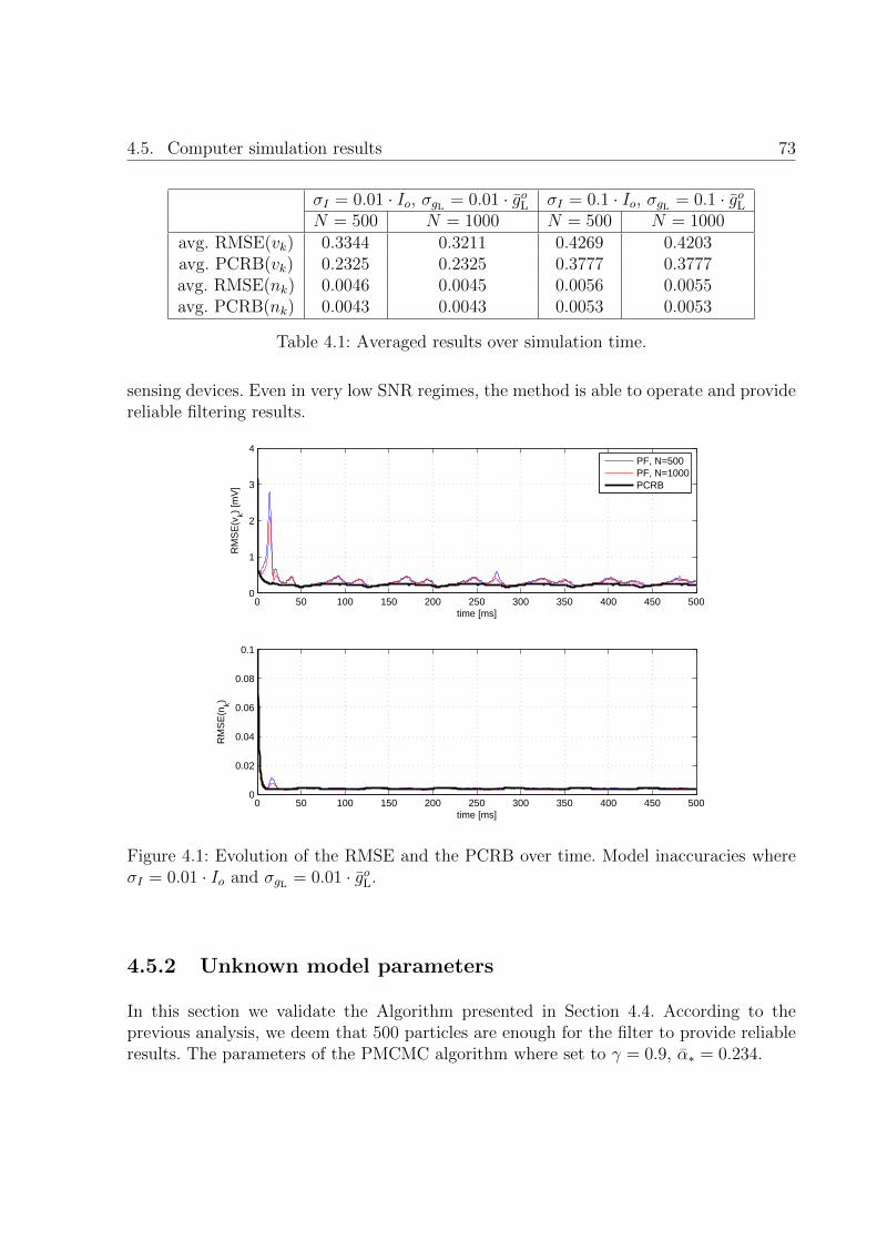
4.5. Computer simulation results 73
σI = 0.01 · Io, σgL = 0.01 · goL σI = 0.1 · Io, σgL = 0.1 · goLN = 500 N = 1000 N = 500 N = 1000
avg. RMSE(vk) 0.3344 0.3211 0.4269 0.4203avg. PCRB(vk) 0.2325 0.2325 0.3777 0.3777avg. RMSE(nk) 0.0046 0.0045 0.0056 0.0055avg. PCRB(nk) 0.0043 0.0043 0.0053 0.0053
Table 4.1: Averaged results over simulation time.
sensing devices. Even in very low SNR regimes, the method is able to operate and providereliable filtering results.
0 50 100 150 200 250 300 350 400 450 5000
1
2
3
4
time [ms]
RM
SE
(vk)
[mV
]
0 50 100 150 200 250 300 350 400 450 5000
0.02
0.04
0.06
0.08
0.1
time [ms]
RM
SE
(nk)
PF, N=500PF, N=1000PCRB
Figure 4.1: Evolution of the RMSE and the PCRB over time. Model inaccuracies whereσI = 0.01 · Io and σgL = 0.01 · goL.
4.5.2 Unknown model parameters
In this section we validate the Algorithm presented in Section 4.4. According to theprevious analysis, we deem that 500 particles are enough for the filter to provide reliableresults. The parameters of the PMCMC algorithm where set to γ = 0.9, α∗ = 0.234.
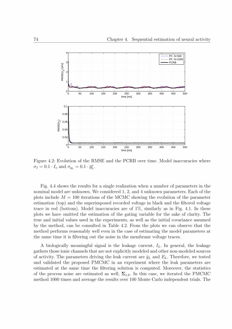
74 Chapter 4. Sequential estimation of neural activity
0 50 100 150 200 250 300 350 400 450 5000
1
2
3
4
time [ms]
RM
SE
(vk)
[mV
]
0 50 100 150 200 250 300 350 400 450 5000
0.02
0.04
0.06
0.08
0.1
time [ms]
RM
SE
(nk)
PF, N=500PF, N=1000PCRB
Figure 4.2: Evolution of the RMSE and the PCRB over time. Model inaccuracies whereσI = 0.1 · Io and σgL = 0.1 · goL.
Fig. 4.4 shows the results for a single realization when a number of parameters in thenominal model are unknown. We considered 1, 2, and 4 unknown parameters. Each of theplots include M = 100 iterations of the MCMC showing the evolution of the parameterestimation (top) and the superimposed recorded voltage in black and the filtered voltagetrace in red (bottom). Model inaccuracies are of 1%, similarly as in Fig. 4.1. In theseplots we have omitted the estimation of the gating variable for the sake of clarity. Thetrue and initial values used in the experiments, as well as the initial covariance assumedby the method, can be consulted in Table 4.2. From the plots we can observe that themethod performs reasonably well even in the case of estimating the model parameters atthe same time it is filtering out the noise in the membrane voltage traces.
A biologically meaningful signal is the leakage current, IL. In general, the leakagegathers those ionic channels that are not explicitly modeled and other non-modeled sourcesof activity. The parameters driving the leak current are gL and EL. Therefore, we testedand validated the proposed PMCMC in an experiment where the leak parameters areestimated at the same time the filtering solution is computed. Moreover, the statisticsof the process noise are estimated as well, Σx,k. In this case, we iterated the PMCMCmethod 1000 times and average the results over 100 Monte Carlo independent trials. The
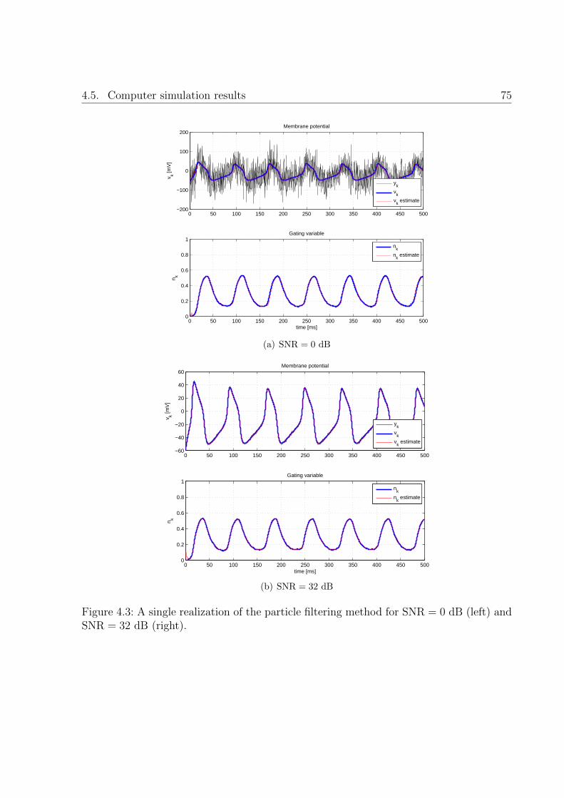
4.5. Computer simulation results 75
0 50 100 150 200 250 300 350 400 450 500−200
−100
0
100
200
v k [mV
]
Membrane potential
yk
vk
vk estimate
0 50 100 150 200 250 300 350 400 450 5000
0.2
0.4
0.6
0.8
1
time [ms]
n k
Gating variable
n
k
nk estimate
(a) SNR = 0 dB
0 50 100 150 200 250 300 350 400 450 500−60
−40
−20
0
20
40
60
v k [mV
]
Membrane potential
yk
vk
vk estimate
0 50 100 150 200 250 300 350 400 450 5000
0.2
0.4
0.6
0.8
1
time [ms]
n k
Gating variable
n
k
nk estimate
(b) SNR = 32 dB
Figure 4.3: A single realization of the particle filtering method for SNR = 0 dB (left) andSNR = 32 dB (right).
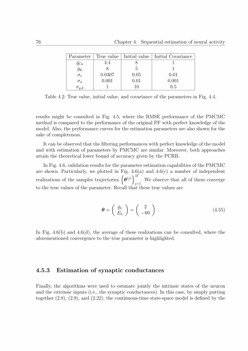
76 Chapter 4. Sequential estimation of neural activity
Parameter True value Initial value Initial CovariancegCa 4.4 8 1gK 8 5 1σv 0.0307 0.05 0.01σn 0.001 0.01 0.001σy,k 1 10 0.5
Table 4.2: True value, initial value, and covariance of the parameters in Fig. 4.4.
results might be consulted in Fig. 4.5, where the RMSE performance of the PMCMCmethod is compared to the performance of the original PF with perfect knowledge of themodel. Also, the performance curves for the estimation parameters are also shown for thesake of completeness.
It can be observed that the filtering performances with perfect knowledge of the modeland with estimation of parameters by PMCMC are similar. Moreover, both approachesattain the theoretical lower bound of accuracy given by the PCRB.
In Fig. 4.6, validation results for the parameter estimation capabilities of the PMCMCare shown. Particularly, we plotted in Fig. 4.6(a) and 4.6(c) a number of independent
realizations of the samples trajectoriesθ(j)Mj=1
. We observe that all of them converge
to the true values of the parameter. Recall that these true values are
θ =
(gLEL
)=
(2−60
). (4.55)
In Fig. 4.6(b) and 4.6(d), the average of these realizations can be consulted, where theaforementioned convergence to the true parameter is highlighted.
4.5.3 Estimation of synaptic conductances
Finally, the algorithms were used to estimate jointly the intrinsic states of the neuronand the extrinsic inputs (i.e., the synaptic conductances). In this case, by simply puttingtogether (2.8), (2.9), and (2.22), the continuous-time state-space model is defined by the

4.5. Computer simulation results 77
Parameter True value Initial value Initial CovarianceτE 2.73 1.5 1gE,0 12.1 10 1σE 12 25 5τI 10.49 15 10gI,0 57.3 45 10σI 26.4 35 5
Table 4.3: True value, initial value, and covariance of the parameters in Fig. 4.8.
following equations
Cmv = −gL(v − EL)− gCam∞(v)(v − ECa)− gKn(v − EK)− Isyn + Iapp (4.56)
n = φn∞(v)− nτn(v)
(4.57)
gE = − 1
τE
(gE − gE,0) +
√2σ2
E
τE
χ (4.58)
gI = − 1
τI
(gI − gI,0) +
√2σ2
I
τI
χ , (4.59)
where Isyn = gE(t)(v(t)−EE)+gI(t)(v(t)−EI). Discretization is straightforward followingSection 4.1, but continuous-time provides here a more compact expression of the system.
First, the method with perfect knowledge of the model (see Algorithm 4.1) was val-idated in Fig. 4.7. It can be observed in Fig. 4.7(a) that the intrinsic signals can beeffectively recovered as before where synaptic inputs where not accounted for. The esti-mation of gE(t) and gI(t) is seen in Fig. 4.7(b). We see that the estimation of the theexcitatory and inhibitory terms is quite accurate, and that the presence of spikes does notdegrade the estimation capabilities of the method.
The PMCMC algorithm (see Algorithm 4.3) was tested in the same experiment. Inthis case, we assumed that the model parameters related to vk and nk where accuratelyestimated, for instance using the procedure described earlier in this chapter. Therefore,we focused on the estimation of those parameters that describe the OU process of each ofthe synaptic terms. Particularly, we considered the values in Table 4.3. The results can beconsulted in Fig. 4.8 and compared to those in Fig. 4.7. We observe that little degradationwith respect to the optimal case of perfectly knowing the model can be identified.
78 Chapter 4. Sequential estimation of neural activity
4.6 Summary
In this chapter we proposed a particle filtering method with optimal importance densitythat is able to sequentially infer the time-course of the membrane potential and the in-trinsic activity of ionic channels from noisy observations of voltage traces. In addition, wetackle the problem of joint parameter estimation and state filtering by extending the de-sign PF with an MCMC procedure. The overall method is iterative. The results show thevalidity of the approaches. The procedure can be applied to any neuron model. Forthcom-ing applications would be validating the method using real data recordings and addingsynaptic terms to the neuron model and use our method to infer the synaptic conduc-tances. The latter problem (addressed in next Chapter) is a challenging hot topic in theneuroscience literature, which is recently focusing on methods to extract the conductancesfrom single-trace measurements, [Bed11], [Kob11]. We think that our PF method wouldgive useful and interesting results to physiologists that aim at inferring brain’s activationrules from neurons’ activities.
4.A. Appendix: PCRB in Morris-Lecar models 79
Appendix 4.A PCRB in Morris-Lecar models
This Appendix is devoted to the derivation of the PCRB estimation bound for the Morris-Lecar model used in this Chapter. We follow the procedure learned in Chapter 3 for thecase of nonlinear states and linear measurements under additive Gaussian noise.
Recall that the state-space we are dealing with is of the form
xk = fk−1(xk−1) + νk
yk = hxk + ek , (4.60)
where h = (1, 0), xk = (vk, nk)>, and fk−1(xk−1) defined by (4.8) and (4.9). The noise
terms are of the form
νk ∼ N (0,Σx,k) (4.61)
ek ∼ N (0, σ2y,k) . (4.62)
In this case, the PCRB can be computed recursively by virtue of Proposition 3.1 with
D11k = Exk
F>k Σ−1
x,kFk
D12k = D21
k = −Exk
F>k
Σ−1x,k
D22k = Σ−1
x,k + H>k+1Σ−1y,k+1Hk+1 . (4.63)
where we D22k becomes deterministic, but the rest of terms involving expectations have
to be computed by Monte Carlo approximations.
Since the state function is nonlinear, we use the Jacobian evaluated at the true valueof xk instead, that is
Fk =[∇xkf>k (xk)
]>=
( ∂f1∂vt
∂f1∂nt
∂f2∂vt
∂f2∂nt
), (4.64)
where functions f1 and f2 are as in (4.8) and (4.9), respectively. Therefore, to evaluatethe bound we need to compute the derivatives in the Jacobian. These are,
∂f1(xk)
∂vk= 1− Ts
Cm
(gL + gKnk + gCa
∂m∞(vk)
∂vkvk + gCam∞(vk)
)(4.65)
∂f1(xk)
∂nk= − Ts
CmgK(vk − EK) (4.66)
∂f2(xk)
∂vk= Tsφ
∂n∞(vk)∂vk
τn(vk)− (n∞(vk−1)− nk−1)∂τn(vk)∂vk
τ 2n(vk)
(4.67)
∂f2(xk)
∂nk= 1− Tsφ
τn(vk)(4.68)
80 Chapter 4. Sequential estimation of neural activity
with
∂m∞(vk)
∂vk=
1
2V2
sech2
(vk − V1
V2
)(4.69)
∂n∞(vk)
∂vk=
1
2V4
sech2
(vk − V3
V4
)(4.70)
∂τn(vk)
∂vk= − 1
2V4
sinh(vk−V3
2V4
)cosh2
(vk−V3
2V4
) . (4.71)
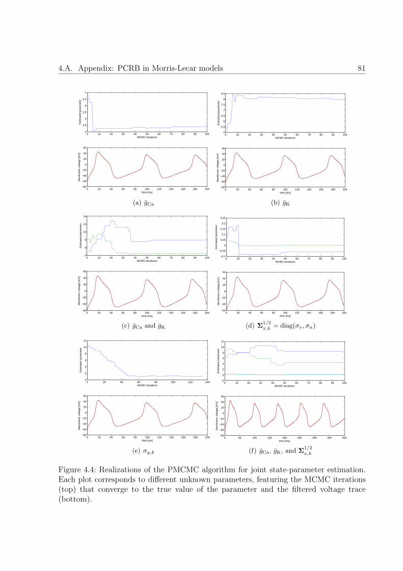
4.A. Appendix: PCRB in Morris-Lecar models 81
0 10 20 30 40 50 60 70 80 90 1004
4.5
5
5.5
6
6.5
7
MCMC iterations
Est
imat
ed p
aram
eter
0 20 40 60 80 100 120 140 160 180 200−80
−60
−40
−20
0
20
40
60
time [ms]
Mem
bran
e vo
ltage
[mV
]
(a) gCa
0 10 20 30 40 50 60 70 80 90 1005
5.5
6
6.5
7
7.5
8
8.5
MCMC iterations
Est
imat
ed p
aram
eter
0 20 40 60 80 100 120 140 160 180 200−80
−60
−40
−20
0
20
40
60
time [ms]
Mem
bran
e vo
ltage
[mV
]
(b) gK
0 10 20 30 40 50 60 70 80 90 1004
6
8
10
12
14
MCMC iterations
Est
imat
ed p
aram
eter
0 20 40 60 80 100 120 140 160 180 200−60
−40
−20
0
20
40
60
time [ms]
Mem
bran
e vo
ltage
[mV
]
(c) gCa and gK
0 10 20 30 40 50 60 70 80 90 100−0.1
−0.05
0
0.05
0.1
0.15
0.2
0.25
MCMC iterations
Est
imat
ed p
aram
eter
0 20 40 60 80 100 120 140 160 180 200−60
−40
−20
0
20
40
60
time [ms]
Mem
bran
e vo
ltage
[mV
]
(d) Σ1/2x,k = diag(σv, σn)
0 20 40 60 80 100 120 1400
2
4
6
8
10
12
MCMC iterations
Est
imat
ed p
aram
eter
0 20 40 60 80 100 120 140 160 180 200−80
−60
−40
−20
0
20
40
60
time [ms]
Mem
bran
e vo
ltage
[mV
]
(e) σy,k
0 10 20 30 40 50 60 70 80 90 100−2
0
2
4
6
8
10
12
MCMC iterations
Est
imat
ed p
aram
eter
0 50 100 150 200 250 300 350 400−80
−60
−40
−20
0
20
40
60
time [ms]
Mem
bran
e vo
ltage
[mV
]
(f) gCa, gK, and Σ1/2x,k
Figure 4.4: Realizations of the PMCMC algorithm for joint state-parameter estimation.Each plot corresponds to different unknown parameters, featuring the MCMC iterations(top) that converge to the true value of the parameter and the filtered voltage trace(bottom).

82 Chapter 4. Sequential estimation of neural activity
0 50 100 150 200 250 3000
0.5
1
1.5
2
2.5
3
3.5
4
time [ms]
RM
SE
(vk)
[mV
]
PF (known model)PMCMC (joint state−parameter estimation)PCRB
(a)
0 50 100 150 200 250 3000
0.01
0.02
0.03
0.04
0.05
0.06
0.07
0.08
0.09
0.1
time [ms]
RM
SE
(nk)
PF (known model)PMCMC (joint state−parameter estimation)PCRB
(b)
Figure 4.5: Evolution of RMSE(vk) (top) and RMSE(nk) (bottom) over time for thePMCMC method estimating the leakage parameters. Model inaccuracies where σI = 0.1·Ioand σgL = 0.1 · goL.

4.A. Appendix: PCRB in Morris-Lecar models 83
0 100 200 300 400 500 600 700 800 900 10001
2
3
4
5
6
7
MCMC iterations
Est
imat
ed p
aram
eter
(a) gL estimates
0 100 200 300 400 500 600 700 800 900 10000
1
2
3
4
5
6
7
8
9
10
MCMC iterations
Est
imat
ed p
aram
eter
(b) Mean gL estimate
0 100 200 300 400 500 600 700 800 900 1000−65
−60
−55
−50
−45
−40
−35
−30
−25
−20
−15
MCMC iterations
Est
imat
ed p
aram
eter
(c) EL estimates
0 100 200 300 400 500 600 700 800 900 1000−70
−60
−50
−40
−30
−20
−10
0
MCMC iterations
Est
imat
ed p
aram
eter
(d) Mean EL estimate
Figure 4.6: Parameter estimation performance of the proposed PMCMC algorithm. Topplots show results for gL = 2 estimation and bottom plots for EL = −60. Left plotsshow superimposed independent realizations and right plots the average estimate of theparameter.
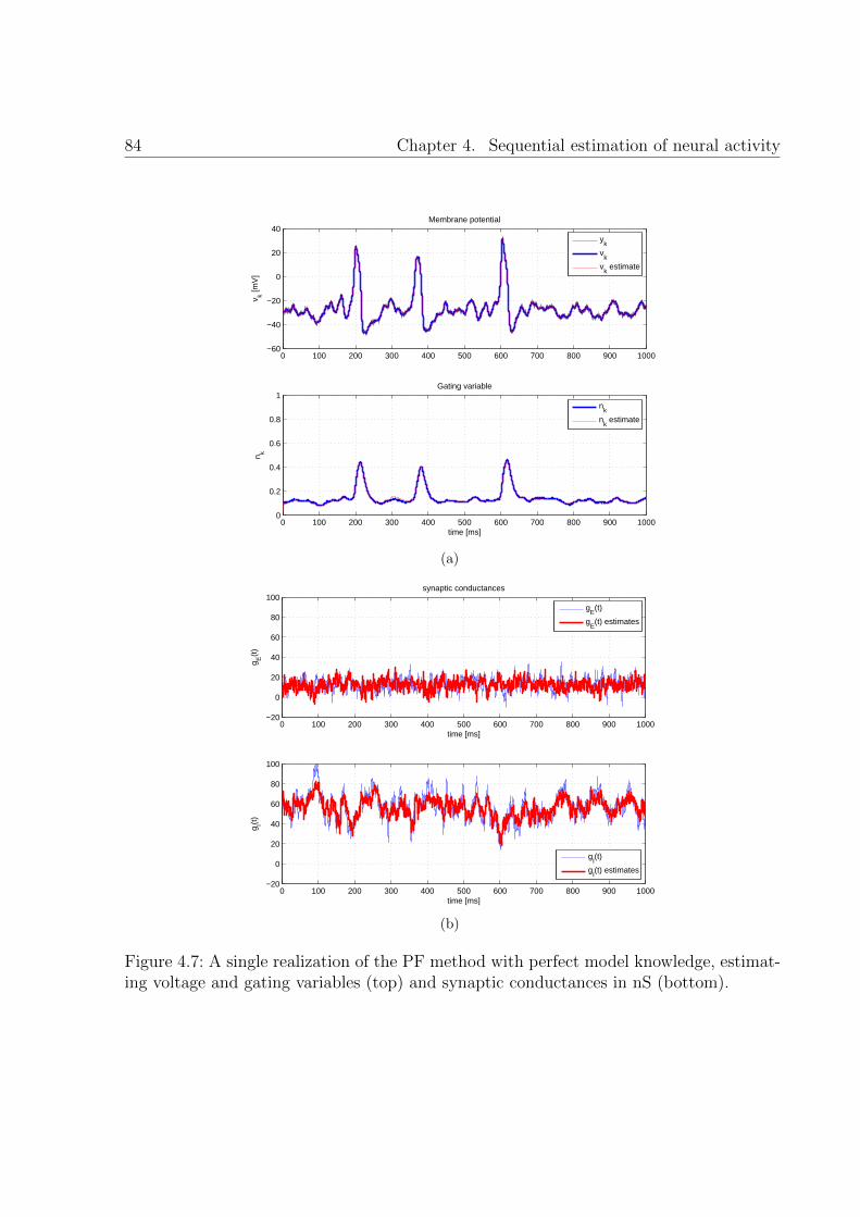
84 Chapter 4. Sequential estimation of neural activity
0 100 200 300 400 500 600 700 800 900 1000−60
−40
−20
0
20
40
v k [mV
]
Membrane potential
0 100 200 300 400 500 600 700 800 900 10000
0.2
0.4
0.6
0.8
1
time [ms]
n k
Gating variable
n
k
nk estimate
yk
vk
vk estimate
(a)
0 100 200 300 400 500 600 700 800 900 1000−20
0
20
40
60
80
100synaptic conductances
g E(t
)
time [ms]
g
E(t)
gE(t) estimates
0 100 200 300 400 500 600 700 800 900 1000−20
0
20
40
60
80
100
g I(t)
time [ms]
gI(t)
gI(t) estimates
(b)
Figure 4.7: A single realization of the PF method with perfect model knowledge, estimat-ing voltage and gating variables (top) and synaptic conductances in nS (bottom).
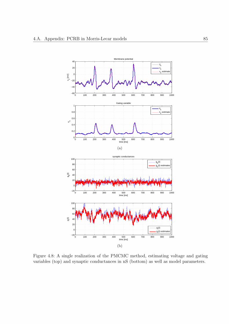
4.A. Appendix: PCRB in Morris-Lecar models 85
0 100 200 300 400 500 600 700 800 900 1000−60
−40
−20
0
20
40
v k [mV
]
Membrane potential
y
k
vk
vk estimate
0 100 200 300 400 500 600 700 800 900 10000
0.2
0.4
0.6
0.8
1
time [ms]
n k
Gating variable
n
k
nk estimate
(a)
0 100 200 300 400 500 600 700 800 900 1000−20
0
20
40
60
80
100synaptic conductances
g E(t
)
time [ms]
g
E(t)
gE(t) estimates
0 100 200 300 400 500 600 700 800 900 1000−20
0
20
40
60
80
100
g I(t)
time [ms]
gI(t)
gI(t) estimates
(b)
Figure 4.8: A single realization of the PMCMC method, estimating voltage and gatingvariables (top) and synaptic conductances in nS (bottom) as well as model parameters.

86 Chapter 4. Sequential estimation of neural activity

5Conclusions and Outlook
THIS Thesis has dealt with the problem of estimating the dynamics of a neuron,its intrinsic signals, and the extrinsic contributions from neighboring neurons. The
experimental setup was presented in Fig. 2.3. The main results and conclusions areherein itemized:
• We reviewed the addressed neuroscience problem, providing some basic factsfor the non-specialist to follow the Thesis and understand the contribution.
• We provided a tutorial review of Bayesian filtering, which is the mathemat-ical tool used along the dissertation. We identified the existing solutions to treatproblems in state-space.
• The experimental problem was discussed, highlighting the impairments intro-duced by the sensing devices that provide the observations. Namely, we discussedthe need to work in the discrete domain and the efficient treatment of noisy obser-vations.
• We designed a method, based on particle filtering, that is able to estimate theionic channel activity and filter out the noise in voltage traces. We havedesigned the particle filter such that it uses the optimal importance density torandomly generate the particles, contrary to other solutions in the literature. This
87
88 Chapter 5. Conclusions and Outlook
method is model-dependent and requires perfect knowledge of its parameters. Themethod attains the initial goals of operating in a single-trial basis, sequentially, inthe presence of spikes, and efficiently.
• To accomplish the targeted robustness goal, we investigated a further improve-ment of the particle filtering algorithm were the parameters of the neural model areestimated from the single-trial voltage trace along with the time-evolving states ofthe neuron. We used the so-called particle MCMC algorithm, which we testedin the problem under study, obtaining promising results. The method attains theinitial goals of operating in a single-trial basis, in the presence of spikes, robustly,and efficiently. The method is not purely sequential, as the MCMC step requires thesuccessive processing of batches of observations, and thus there is a need for storinga set of data.
• We were able to show, by realistic computer simulation experiments, that the meth-ods are able to recover the intrinsic activity of a neuron and the extrinsic inputs,i.e. the synaptic conductances.
• To benchmark the filtering solutions, we derived the PCRB for the system. This isof particular relevance since no other work in the literature has derived it, and thuscompared their results to those provided by the fundamental estimation bounds. Wederived the PCRB for the state-space system based on the Morris-Lecar neuralmodel, but it could be straightforwardly derived for other neuron models.
• In summary, the reported work goes beyond the state-of-the-art in the esti-mation of neural activity, both providing novel filtering solutions and deriving thebenchmark bounds.
Due to time limitations, there are a number of topics that we were not able to addressor investigate further in this Thesis. Therefore, the following is a list of future researchtopics that are a result of the work reported in this dissertation:
• The filtering tools proposed in this Thesis should be further investigated in thecontext of synaptic conductance estimation. Here we only draw some preliminaryresults, but more exhaustive analysis are required.
• Use the methods with real data to show the benefits of the tools derived in thiswork.
• The parameter estimation procedure is not on-line. A further improvement couldbe to study purely on-line methods such as the on-line EM.

89
• From an algorithmic point of view, one may argue that under the Gaussian assump-tion one might use solutions based on SPKF methods. This would eventuallyproduce savings in the computational complexity of the algorithm, which in thecase of PF is rather high. Future work could be addressed to the comparison of suchapproaches to the ones based on particle filtering that are considered here.
• The inference methods herein proposed are model-dependent. Even the algorithmthat is able to estimate the parameters of the model needs a model. Sometime itis not possible to identify which of the plethora of neural mathematical modelsto select (e.g., Morris-Lecar, HodgkinHuxley, Fitz-Nagumo,etc.). In the Bayesianparadigm it is natural to let the method know that we have several options forthe model themselves. Therefore, future work could be in the incorporation of theso-called Interating Multiple Model structures in the proposed algorithms.
• We did some preliminary tests with the smoothing versions of the proposed filters.The results were promising and could be further investigated.

90 Chapter 5. Conclusions and Outlook
Bibliography
[And79] B. D. O. Anderson, and J. B. Moore, Optimal Filtering , Prentice–Hall, 1979.
[And04] C. Andrieu, Arnaud Doucet, S.S. Singh, and V.B. TADIC, “Particle methodsfor change detection, system identification, and control”, Proceedings of theIEEE , vol. 92, no. 3, pp. 423–438, Mar 2004.
[And05] C. Andrieu, Arnaud Doucet, and Vladislav B. Tadic, “On-line parameter esti-mation in general state-space models”, Decision and Control, 2005 and 2005European Control Conference. CDC-ECC ’05. 44th IEEE Conference on, pp.332–337, Dec 2005.
[And10] C. Andrieu, A. Doucet, and R. Holenstein, “Particle Markov chain Monte Carlomethods”, Journal of the Royal Statistical Society Series B , vol. 72, no. 3,pp. 269–342, 2010.
[Ara07] I. Arasaratnam, S. Haykin, and R. J. Elliot, “Discrete-time nonlinear filteringalgorithms using Gauss-Hermite quadrature”, Proc. of the IEEE , vol. 95, no. 5,pp. 953–977, 2007.
[Ara08] I. Arasaratnam, and S. Haykin, “Square–Root Quadrature Kalman Filtering”,IEEE Trans. Signal Processing , vol. 56, no. 6, pp. 2589–2593, June 2008.
[Ara09] I. Arasaratnam, and S. Haykin, “Cubature Kalman Filters”, IEEE Trans. Au-tomatic Control , vol. 54, no. 6, pp. 1254–1269, June 2009.
[Aru02] S. Arulampalam, S. Maskell, N. Gordon, and T. Clapp, “A Tutorial on ParticleFilters for Online Nonlinear/Non-Gaussian Bayesian Tracking”, IEEE Trans.Signal Processing , vol. 50, no. 2, pp. 174–188, February 2002.
[Bed11] C. Bedard, S. Behuret, C. Deleuze, T. Bal, and A. Destexhe, “Oversamplingmethod to extract excitatory and inhibitory conductances from single-trialmembrane potential recordings.”, Journal of neuroscience methods , set. 2011.
91
92 Bibliography
[Bay63] T. Bayes, “An essay towards solving a problem in the doctrine of chances”, ThePhilosophical Transactions of the Royal Society of London, vol. 53, pp. 370–418,1763.
[Ber97] C. Berzuini, N. Best, W. Gilks, and C. Larizza, “Dynamic conditional indepen-dence models and Markov chain Monte Carlo methods”, Journal of AmericanStat. Assoc., vol. 92, pp. 1403–1412, 1997.
[Ber99] N. Bergman, Recursive Bayesian Estimation: Navigation and Tracking Appli-cations , PhD Thesis, Linkopings Universitet, Sweden, 1999.
[Ber01] N. Bergman, A. Doucet, and N. Gordon, “Optimal estimation and Cramer-Raobounds for partial non-Gaussian state space models”, Ann. Inst. Statist. Math.,vol. 53, no. 1, pp. 97–112, 2001.
[Bob75] B. Z. Bobrovsky, and M. Zakai, “A lower bound on the estimation error forMarkov processes”, IEEE Trans. Automat. Contr., vol. 20, no. 6, pp. 785–788,December 1975.
[Bol04a] M. Bolic, Architectures for Efficient Implementation of Particle Filters , PhDThesis, Stony Brook University, New York, August 2004.
[Bol04b] M. Bolic, P. Djuric, and S. Hong, “Resampling algorithms for particle filters: Acomputational complexity perspective”, EURASIP Journal on Applied SignalProcessing , , no. 15, pp. 2267–2277, 2004.
[Bol05] M. Bolic, P. M. Djuric, and S. Hong, “Resampling Algorithms and Architecturesfor Distributed Particle Filters”, IEEE Trans. Signal Processing , vol. 53, no. 7,pp. 2442–2450, July 2005.
[Bre12] Romain Brette, and Alain Destexhe, Handbook of Neural Activity Measurement ,Cambridge University Press, 2012.
[Bro11] S. Brooks, A. Gelman, G. Jones, and X. Meng, “Handbook of Markov ChainMonte Carlo”, 2011.
[Bug07] M. F. Bugallo, T. Lu, and P. M. Djuric, “Target Tracking by Multiple ParticleFiltering”, Proc. of IEEE Aerospace Conference, Big Sky, MT, USA, March2007.
[Cev07] V. Cevher, R. Velmurugan, and J. H. McClellan, “Acoustic multitarget track-ing using direction-of-arrival batches”, IEEE Trans. Signal Processing , vol. 55,no. 6, pp. 2810–2825, June 2007.
Bibliography 93
[Che03] Z. Chen, “Bayesian filtering: From Kalman filters to particle filters, and be-yond”, Tech. rep., Adaptive Syst. Lab., McMaster University, Ontario, Canada,2003.
[Clo09] P. Closas, Bayesian Signal Processing Techniques for GNSS Receivers: frommultipath mitigation to positioning , PhD Thesis, Dept. of Signal Theory andCommunications, Universitat Politecnica de Catalunya (UPC), Barcelona,Spain, June 2009.
[Clo12a] P. Closas, and M. F. Bugallo, “Improving Accuracy by Iterated Multiple Parti-cle Filtering”, IEEE Signal Processing Lett., vol. 19, no. 8, pp. 531–534, August2012.
[Clo12b] P. Closas, C. Fernandez-Prades, and J. Vila-Valls, “Multiple QuadratureKalman Filtering”, Signal Processing, IEEE Transactions on, vol. 60, no. 12,pp. 6125–6137, Dec 2012.
[Clo13a] P. Closas, and A. Guillamon, “Estimation of neural voltage traces and associ-ated variables in uncertain models”, BMC Neuroscience, vol. 14, no. 1, pp. 1151,July 2013.
[Clo13b] P. Closas, and A. Guillamon, “Sequential estimation of gating variables fromvoltage traces in single-neuron models by particle filtering”, Proceedings of theIEEE International Conference on Acoustics, Speech, and Signal Processing,ICASSP 2013 , Vancouver, Canada, May 2013.
[Cri01] D. Crisan, Sequential Monte Carlo methods in Practice, Chap. Particle Filters- A theoretical perspective, pp. 17–41, Springer-Verlag, 2001.
[Cri02] D. Crisan, and A. Doucet, “A Survey of Convergence Results on Particle Filter-ing for Practitioners”, IEEE Trans. Signal Processing , vol. 50, no. 3, pp. 736–746, March 2002.
[Dau03] F. Daum, and J. Huang, “Curse of dimensionality and particle filters”, Proc. ofIEEE Aerospace Conference, vol. 4, pp. 1979–1993, Big Sky, MT, USA, March2003.
[Day05] Peter Dayan, and L. F. Abbott, Theoretical Neuroscience: Computational andMathematical Modeling of Neural Systems , The MIT Press, 2005.
[Dju03] P. M. Djuric, J. H. Kotecha, J. Zhang, Y. Huang, T. Ghirmai, M. F. Bugallo,and J. Mıguez, “Particle Filtering”, IEEE Signal Processing Mag., vol. 20, no. 5,pp. 19–38, September 2003.

94 Bibliography
[Dou98] A. Doucet, “On Sequential Simulation–Based Methods for Bayesian Filtering”,Tech. Rep. CUED/F-INFENG/TR.310, University of Cambridge, 1998.
[Dou00] A. Doucet, S. J. Godsill, and C. Andrieu, “On sequential Monte Carlo samplingmethods for Bayesian filtering”, Stat. Comput., vol. 3, pp. 197–208, 2000.
[Dou01a] A. Doucet, N. de Freitas, and N. Gordon (eds.), Sequential Monte Carlo Methodsin Practice, Springer, 2001.
[Dou01b] A. Doucet, N. De Freitas, and N. Gordon (eds.), Sequential Monte Carlo meth-ods in practice, Springer, 2001.
[Dou05] R. Douc, O. Cappe, and E. Moulines, “Comparison of resampling schemes forparticle filtering”, Proc. of the 4th International Symposium on Image and Sig-nal Processing and Analysis, ISPA’05 , pp. 64–69, Zagreb, Croatia, Sept. 2005.
[Erm10] B. Ermentrout, D. Terman, “Mathematical Foundations of Neuroscience”, NewYork: Springer, 2010. ISBN 978-0-387-87708-2.
[Fit61] R. FitzHugh, “Impulses and physiological states in theoretical models of nervemembrane”, Biophys. J., vol. 1, pp. 445–466, 1961.
[Gew89] J. Geweke, “Bayesian inference in econometric models using Monte Carlo inte-gration”, Econometrica, vol. 24, pp. 1317–1399, 1989.
[Gil96] W.R. Gilks, S. Richardson, and D.J. Spiegelhalter (eds.), Markov Chain MonteCarlo in Practice: Interdisciplinary Statistics , CRC Interdisciplinary StatisticsSeries, Chapman & Hall, 1996.
[God01] S. Godsill, and T. Clapp, Sequential Monte Carlo methods in Practice, Chap.Improvement strategies for Monte Carlo particle filters, pp. 139–158, Springer-Verlag, 2001.
[Gol73] G. Golub, and V. Pereyra, “The differentiation of pseudo-inverses and nonlin-ear least squares problems whose variables separate”, SIAM J. Numer. Anal.,vol. 10, pp. 413–432, 1973.
[Gol96] G. H. Golub, and C. F. van Loan, Matrix Computations , The John HopkinsUniversity Press, 3rd ed., 1996.
[Gor93] N. Gordon, D. Salmond, and A. Smith, “A novel approach to nonlinear/non-Gaussian Bayesian state estimation”, IEE Proceedings on Radar and SignalProcessing , vol. 140, pp. 107–113, 1993.
Bibliography 95
[Gui06] Antoni Guillamon, David W. McLaughlin, and John Rinzel, “Estimation ofsynaptic conductances.”, Journal of physiology, Paris , vol. 100, no. 1-3, pp. 31–42, 2006.
[Ham54] J. M. Hammersley, and K. W. Morton, “Poor man’s Monte Carlo”, Journal ofthe Royal Statistical Society , vol. 16, pp. 23–38, 1954.
[Hen08] G. Hendeby, Performance and Implementation Aspects of Nonlinear Filtering ,PhD Thesis, Linkopings Universitet, Linkoping, Sweden, 2008.
[Hig95] T. Higuchi, “Kitagawa monte carlo filter from the perspective of genetic algo-rithm”, Research memorandum, The Institute of Statistical Mathematics, 1995.
[Hod52] A. L. Hodgkin, and A. F. Huxley, “The components of membrane conductancein the giant axon of Loligo”, J Physiol., vol. 116, no. 4, pp. 473–496, April 1952.
[Ito00] K. Ito, and K. Xiong, “Gaussian Filters for Nonlinear Filtering Problems”,IEEE Trans. Automat. Contr., vol. 45, no. 5, May 2000.
[Izh04] E.M. Izhikevich, “Which model to use for cortical spiking neurons?”, NeuralNetworks, IEEE Transactions on, vol. 15, no. 5, pp. 1063–1070, Sept 2004.
[Izh06] E. Izhikevich, Dynamical systems in neuroscience: the geometry of excitabilityand bursting , MIT Press, Cambridge, MA, 2006.
[Jaz70] A. H. Jazwinski, Stochastic Processes and Filtering Theory , vol. 64 of Mathe-matics in Science and Engineering , Academic Press, 1970.
[Jul97] S. Julier, and J. K. Uhlmann, “A new extension of the Kalman filter to nonlinearsystems”, Int. Symp. Aerospace/Defense Sensing, Simul. and Controls , vol. 3,1997.
[Jul00] S. Julier, J. Uhlmann, and H. F. Durrant-White, “A new method for nonlineartransformation of means and covariances in filters and estimators”, IEEE Trans.Automat. Contr., vol. 45, pp. 477–482, March 2000.
[Jul04] S. J. Julier, and J. K. Ulhmann, “Unscented filtering and nonlinear estimation”,Proc. of the IEEE , vol. 92, no. 3, pp. 401–422, March 2004.
[Kal60] R. E. Kalman, “A new approach to linear filtering and prediction problems”,Transactions of the ASME-Journal of Basic Engineering , vol. 82, no. Series D,pp. 35–45, 1960.
[Kar05] R. Karlsson, Particle Filtering for Positioning and Tracking Applications , PhDThesis, Linkopings Universitet, Linkoping, Sweden, March 2005.
96 Bibliography
[Kay93] S. M. Kay, Fundamentals of Statistical Signal Processing. Estimation Theory ,Prentice Hall, 1993.
[Kee09] James P. Keener, and James Sneyd, Mathematical physiology. I. , Cellular phys-iology , Interdisciplinary applied mathematics, Springer, New York, London,2009.
[Kit96] G. Kitakawa, “Monte Carlo filter and smoother for non-Gaussian non-linearstate space models”, Journal of Computational and Graphical Statistics , vol. 5,pp. 1–25, 1996.
[Kob11] R. Kobayashi, Y. Tsubo, P. Lansky, and S. Shinomoto, “Estimating time-varying input signals and ion channel states from a single voltage trace of aneuron”, Advances in Neural Information Processing Systems (NIPS), vol. 24,pp. 217–225, 2011.
[Kon94] A. Kong, J. S. Liu, and W. H. Wong, “Sequential imputations and Bayesianmissing data problems”, Journal of the American Stat. Assoc., vol. 89, no. 425,pp. 278–288, 1994.
[Kot03a] M. Kotecha, and P. M. Djuric, “Gaussian Particle Filtering”, IEEE Trans.Signal Processing , vol. 51, no. 10, pp. 2592–2601, October 2003.
[Kot03b] M. Kotecha, and P. M. Djuric, “Gaussian Sum Particle Filtering”, IEEE Trans.Signal Processing , vol. 51, no. 10, pp. 2602–2610, October 2003.
[Lan13] M. Lankarany, W. P. Zhu, M. N. S. Swamy, and Taro Toyoizumi, “Inferringtrial-to-trial excitatory and inhibitory synaptic inputs from membrane potentialusing Gaussian mixture Kalman filtering”, Frontiers in Computational Neuro-science, vol. 7, 2013.
[Lan14] M. Lankarany, W.-P. Zhu, and M.N.S. Swamy, “Joint estimation of states andparameters of hodgkinhuxley neuronal model using kalman filtering”, Neuro-computing , vol. 136, pp. 289 – 299, 2014.
[Liu95] J. S. Liu, and R. Chen, “Blind deconvolution via sequential imputations”, Jour-nal of the American Stat. Assoc., vol. 90, pp. 567–576, 1995.
[Liu98] J. S. Liu, and R. Chen, “Sequential Monte Carlo methods for dynamical prob-lems”, Journal of the American Stat. Assoc., vol. 93, pp. 1032–1044, 1998.
[Liu08] Jun S. Liu, Monte Carlo Strategies in Scientific Computing , Springer, jan. 2008.
Bibliography 97
[Mıg04] J. Mıguez, M. F. Bugallo, and P. M. Djuric, “A new class of particle filters forrandom dynamic systems with unknown statistics”, EURASIP J. Appl. SignalProcessing , vol. 2004, no. 15, pp. 2278–2294, 2004.
[McG00] S. McGinnity, and G. W. Irwin, “Multiple Model Bootstrap Filter for maneu-vering target tracking”, IEEE Trans. Aerosp. Electron. Syst., vol. 36, pp. 1006–1012, 2000.
[McL00] D. McLaughlin, R. Shapley, M. Shelley, and D. J. Wielaard, “A neuronal net-work model of macaque primary visual cortex (V1): orientation selectivity anddynamics in the input layer 4Calpha.”, Proceedings of the National Academy ofSciences of the United States of America, vol. 97, no. 14, pp. 8087–8092, jul.2000.
[Mer00] R. Van der Merwe, A. Doucet, N. Freitas, and E. Wan, “The unscented par-ticle filter”, Tech. Rep. CUED/F-INFENG/TR 380, University of Cambridge,August 2000.
[Mer03] R. Van Der Merwe, and E. Wan, “Sigma-Point Kalman Filters for ProbabilisticInference in Dynamic State-Space Models”, Proceedings of the Workshop onAdvances in Machine Learning , Montreal, Canada, June 2003.
[Mor81] C. Morris, and H. Lecar, “Voltage Oscillations in the barnacle giant musclefiber”, Biophys J., vol. 35, no. 1, pp. 193–213, July 1981.
[Mus00] C. Musso, N. Oudjane, and F. Le Gland, Sequential Monte Carlo methods inPractice, Chap. Improving Regularised Particle Filters, pp. 247–272, Springer-Verlag, 2000.
[Nag62] J. Nagumo, S. Arimoto, and S. Yoshizawa, “An active pulse transmission linesimulating nerve axon”, Proceeding IRE , vol. 50, pp. 2061–2070, 1962.
[Nor00] M. Norgaard, N. K. Poulsen, and O. Ravn, “New developments in state esti-mation of nonlinear systems”, Automatica, vol. 36, pp. 1627–1638, 2000.
[Pan12] Liam Paninski, Michael Vidne, Brian DePasquale, and Daniel Gil Ferreira, “In-ferring synaptic inputs given a noisy voltage trace via sequential Monte Carlomethods”, Journal of Computational Neuroscience, vol. 33, no. 1, pp. 1–19,2012.
[Pap01] A. Papoulis, and S. U. Pillai, Probability, Random Variables and StochasticProcesses , McGraw–Hill, New Delhi, India, 4th ed., 2001.
[Pit01] M. Pitt, and N. Shephard, Sequential Monte Carlo methods in Practice, Chap.Auxiliary variable based particle filters, pp. 273–294, Springer-Verlag, 2001.
98 Bibliography
[Piw04] M. Rudolph Z. Piwkowska, M. Badoual, T. Bal, and A. Destexhe, “A methodto estimate synaptic conductances from membrane potential fluctuations”, J.Neurophysiol., no. 91, pp. 2884–2896, 2004.
[Pos08] Martin Pospischil, Maria Toledo-Rodriguez, Cyril Monier, Zuzanna Piwkowska,Thierry Bal, Yves Fregnac, Henry Markram, and Alain Destexhe, “Minimalhodgkin-huxley type models for different classes of cortical and thalamic neu-rons.”, Biological Cybernetics , vol. 99, no. 4-5, pp. 427–441, 2008.
[Pot63] J. E. Potter, and R. G. Stern and, “Statistical filtering of space navigationmeasurements”, Proceedings of the AIAA Guidance, Navigation, and ControlConference, Cambridge, MA, August 1963.
[Poy11] George Poyiadjis, Arnaud Doucet, and Sumeetpal S. Singh, “Particle approx-imations of the score and observed information matrix in state space modelswith application to parameter estimation”, Biometrika, no. 98, pp. 65–80, 2011.
[Pun03] E. Punskaya, Sequential Monte Carlo Methods for digital communications , PhDThesis, University of Cambridge, UK, July 2003.
[Rin98] J. R. Rinzel, and G. B. Ermentrout, “Analysis of neural excitability and oscil-lations”, C. Koch, I. Segev (eds.), Methods in Neural Modeling , pp. 135–169,MIT Press., Cambridge, MA, 1998.
[Ris04] B. Ristic, S. Arulampalam, and N. Gordon, Beyond the Kalman Filter: ParticleFilters for tracking applications , Artech House, Boston, 2004.
[Rub88] D. B. Rubin, J. M. Bernardo, M. H. De Groot, D. V. Lindley, and A. F. M.Smith, Bayesian Statistics 3 , Oxford: University Press, 1988.
[Rud03] M. Rudolph, and A. Destexhe, “Characterization of subthreshold voltage fluctu-ations in neuronal membranes”, Neural Comput., vol. 15, no. 11, pp. 2577–2618,nov. 2003.
[Sar13] S. Sarkka, Bayesian Filtering and Smoothing , Cambridge University Press, NewYork, NY, USA, 2013.
[Sch05] T. Schon, F. Gustafsson, and P.J. Nordlund, “Marginalized particle filters formixed linear/nonlinear state-space models”, IEEE Trans. Signal Processing ,vol. 53, no. 7, pp. 2279–2289, July 2005.
[Sim01] M. Simandl, J. Kralovec, and P. Tichavsky, “Filtering, predictive, and smooth-ing Cramer-Rao bounds for discrete-time nonlinear dynamic systems”, Auto-matica, vol. 37, pp. 1703–1716, 2001.

Index 99
[Sor88] H. Sorenson, Recursive estimation for nonlinear dynamic systems , New York:Marcel Dekker, 1988.
[Spe02] “Special Issue on Monte Carlo methods for Statistical Signal Processing”, IEEETrans. Signal Processing , vol. 50, no. 2, February 2002.
[Str71] A. H. Stroud, Approximate calculation of multiple integrals , Prentice–Hall, En-glewood Cliffs, NJ, 1971.
[Tao04] Louis Tao, Michael Shelley, David Mclaughlin, and Robert Shapley, “An egal-itarian network model for the emergence of simple and complex cells in visualcortex.”, Proc. Natl. Acad. Sci. USA, vol. 101, no. 1, pp. 366–371, jan. 2004.
[Tic98] P. Tichavsky, C. .H. Muravchik, and A. Nehorai, “Posterior Cramer-RaoBounds for Discrete-Time Nonlinear Filtering”, IEEE Trans. Signal Process-ing , vol. 46, no. 5, pp. 1386–1396, May 1998.
[Tre68] Harry L. Van Trees, Part I of Detection, Estimation and Modulation Theory ,Wiley Interscience, New York, 1968.
[Tre07] Harry L. Van Trees, and Kristine L. Bell (eds.), Bayesian Bounds for ParameterEstimation and Nonlinear Filtering/Tracking , Wiley Interscience, 2007.
[Van01] R. Van der Merwe, and E. A. Wan, “The square–root unscented Kalman filterfor state and parameter estimation”, Proceedings of ICASSP’01 , vol. 6, pp.3461–3464, Salt Lake City, UT, May 2001.
[Vih12] Matti Vihola, “Robust adaptive metropolis algorithm with coerced acceptancerate.”, Statistics and Computing , vol. 22, no. 5, pp. 997–1008, 2012.
[Wan00] E. Wan, and R. Van der Merwe, “The unscented kalman filter for nonlinear esti-mation”, IEEE Symp. Adaptive Systems for Signal Proc., Comm. and Control ,pp. 153–158, Alberta, Canada, 2000.
[Wie01] D. J. Wielaard, M. Shelley, D. McLaughlin, and R. Shapley, “How Simple CellsAre Made in a Nonlinear Network Model of the Visual Cortex”, Journal ofNeuroscience, vol. 21, pp. 5203–5211, 2001.
Index
Bayesalgorithms, 35rule, 44
Bayesian Information Matrix, 28
Central Difference filter, 35Chapman-Kolmogorov equation, 26, 44Cubature Kalman filter, 35, 46
Divided Difference filter, 35
EKF, see Extended Kalman FilterExtended Kalman Filter, 37Extended Kalman filter, 35
filtering, 28filtering distribution, 26
Hidden Markov model, 25
importance density, 55optimal, 55suboptimal choices, 56
Importance Sampling, 50Intracellular recordings, 13ionic channel, 7
gating variable, 8
Kalman Filter, 35Kalman filter, 35KF, see Kalman Filter
Maximum a posteriori estimator, 27membrane potential, 6–8, 13, 60Minimum Mean Square Error estimator, 27
Monte-Carlo integration, 49
Nernst potential, 7neuron, 6
axon, 7conductance-based models, 8dendrites, 6HodgkinHuxley model, 9leakage, 8models, 9Morris Lecar model, 10, 24soma, 6synapses, 7synaptic conductances, 8, 12, 76
neuroscience, 5
Ornstein-Uhlenbeck process, 12, 17
Particle Filterconvergence, 53importance density, 55resampling, 53tutorial, 49
particle filter, 35, 63particle MCMC, 66, 68Posterior Cramer-Rao Bound
basics, 28Morris-Lecar, 79recursive, 30
posterior distribution, 25prediction, 28
Quadrature Kalman filter, 35, 47
100
Index 101
Sequential Importance Sampling, 51Sigma-point Kalman filter, 35smoothing, 28state-space
discrete state-space model, 24state-space model, 24
Trajectory Information Matrix, 30
UKF, see Unscented Kalman FilterUnscented Kalman filter, 35, 46