M A S T P R O J E C T 1: W A V E S G 8 - M

Comparison of computations with Boussinesq-like models and laboratory measurements

M.W. Dingemans

H1684.12

July 29, 1994

1 Introduction 2

2 The measurements 5

3 The mathematical models 8

3.1 Danish Hydraulic Institute (DHI) 8 3.2 Delft Hydraulics (WL) 9 3.3 University of Groningen (UG) 10 3.4 Aristotle University of Thessaloniki (AUT) 10 3.5 LEGI-IMG Grenoble 11 3.6 Snamprogetti (Snam) 13 3.7 Technical University Delft (TUD) 13 3.8 Other wave propagation raodels 13

4 Comparison of computations with measurements 13 4.1 Measurement condition A 14

4.1.1 D H I results 14 4.1.2 Delft Hydraulics and University of Groningen results 16

4.1.3 Legi results 16 4.1.4 Snamprogetti results 20 4.1.5 University of Thessaloniki results . 20 4.1.6 A Hamiltonian and a Boundary Element model 20 4.1.7 Results of Technical University Delft 23

4.2 Measurement condition B 23

4.3 Measurement condition C 25

5 Discussion and recommendations 27

In this note results of the comparison between computation of Boussinesq-like models and measurements in a wave flume is given. Purpose of the exercise is to enhance the usability of the models of the various institutes.

1

1. Introduction. I t is already known for a long time that one of the major discrepancies between computations with Boussinesq-like models and measurements, is due to the inac­curate representation of the linear frequency dispersion in the Boussinesq-like long wave models. A comparison of various models as given in Dingemans (1973) showed already large differences between the frequency dispersion of various models. A com­parison with measurements in a flume (Dingemans, 1976) showed that the computed wave profiles were also found in the measurements, but at a different location. This was ascribed to the inaccurate frequency dispersion.

Recently Madsen et al. (1991) took up a suggestion of Witt ing (1984) and suggested a form of Boussinesq-like equations with a much improved frequency dis­persion. This is based upon a [1/1] Fade expansion in the expansion parameter [kKf of the Hnear expression for the square of the phase velocity, c , and the corrre-sponding set of differential equations is sought for then. Madsen et al. (1991, 1992) performed this task by adding higher-order terms consisting of third derivatives in t and X to the horizontal momentum equation. As shown in a lecture by Dingemans (1992) at the final Mast-G6M Workshop in Pisa, a somewhat more systematic way by means of operator correspondence gives various possible models, one of which was given by Madsen et al. (1991). (A written account can be found in Dingemans, 1994). A similar approach is given by Mooiman (1991) who considers a Fadé ap­proximation of c, yielding a slightly less good agreement as does the approximation oic\

For engineering practice it is highly desirable to be able to treat as short waves as possible, although the Boussinesq approximation is strictly valid only for (fairly) long waves. A Fadé expansion of order [1/1] then gives the best possible result without introducing still higher derivatives than the third.

As argued above, deviations between computations and measurements occur for short wave components when these components are freely moving, that is when the components are moving according to their dispersion characteristics. Non-linear waves have the typical characteristic that many components are phase-locked and higher harmonics then travel with the velocity of the basic wave, which velocity is determined by some non-linear correction of the linear dispersion relation. Perma­nent wave forms are possible when the frequency and amplitude dispersion effects balance each other. An example of a permanent wave form is a cnoidal wave in which all higher harmonics are phase-locked. When such a cnoidal wave progresses up a slope, then occasionally an adiabatic approximation is used to describe the shoal­ing process and i t is assumed that the parameters describing the cnoidal wave are changing slowly, but the wave form remains of cnoidal shape. In such an adiabatic approximation all wave components are therefore supposed to remain phase-locked. In general this is not true. A generation of more higher harmonics gives always both free and locked harmonics. This phenomenon becomes especially apparent when the depth is increasing again so that the difference between the phase velocitites of the bound and the free components increases.

Above remarks can be substantiated in the following way. For the decreasing-depth situation the parameter kh also decreases, where k is the wave number of the primary wave. As for long waves the phase velocity in the computational model changes little from the exact linear one, the free waves propagate with a velocity

2

near to the one of the primary wave, and i t takes a long distance before differences become visible. On the backward slope the depth is increasing fast and so does the parameter kh. For larges values of kh the difference between the computational phase velocity and the exact one increases and the free waves have a velocity which deviates much more from the one of the basic wave than for the shallower depth. Because of the phase differences between free and locked higher harmonics soon differences in wave profiles between computations and measurements wi l be visible.

A discriminating test between various models based on Boussinesq-like approx­imations is then provided by a bar-type geometry. On the upward slope effects of non-linearity generate higher harmonics and on the downward slope the difference between locked and free modes becomes clearly visible.

A number of flume and basin experiments based on a bar-type geometry for fairly long waves have become available in the past decade. Some measurements of Dingemans (1976) are also available, but in less detail and of a much less dis­criminating nature (waves on a shelf). In a number of measurements a trapezoidal bar has been taken into consideration, in which the offshore slope is 1 : 20 and the shoreward slope 1 : 10, while the depth in the horizontal depth parts is 40 cm and on the horizontal part of the bar (of extent 2 m) the depth is 10 cm. Such a geometry has been used by Dingemans (1987) in a verification study of the wave propagation model HISWA and by Beji and Battjes in a flume experiment at Delft University of Technology, see Battjes and Beji (1993) and by Liberatore and Fetti (1992) in a flume in Padua.

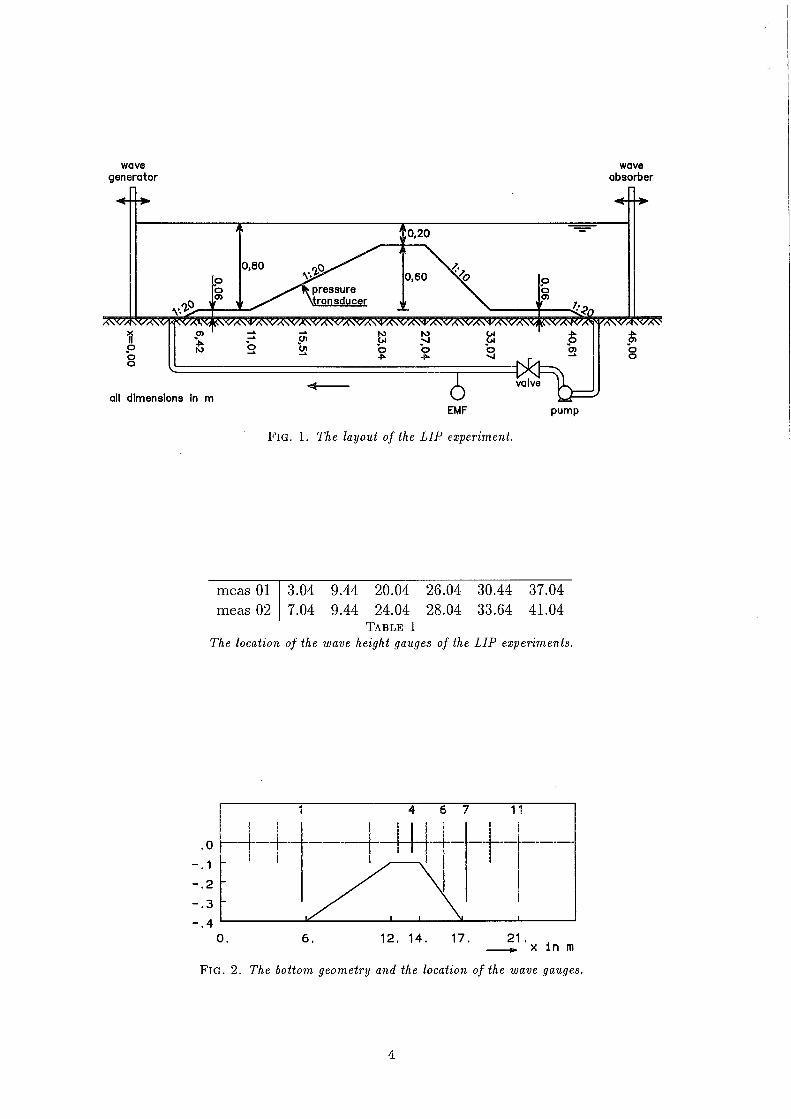
Recently, January 1993, Gert Klopman of Delft Hydraulics has performed three regular wave tests already done by Beji, but with a linear scale of 2, i.e., an undis­turbed depth of 80 cm and 20 cm depth above the bar. Care has been exercised to ensure that exactly the same conditions were performed, i.e., also a wave period T = 2.02V^s has been taken. In the experiments of Klopman, performed as part of the LIP programme, a number of tests with following current have been performed and also information about long bound waves is present. The experiments to be used in the present study do have active wave absorption and also compensation for bound long waves. As the boundary conditions of the wave board and the reflection from the beach have been taken care of very accurately, we wil l use these measure­ments here. The set-up of the experiments is the same as the one reported in Luth et al. (1994). The layout is given in Figure 1 and the placement of the wave gauges is given in Table 1.

For the measurements we use the linear scale factor of 2 so that the results are directly comparable to the measurements of Battjes and Beji and also to the various computations.

We consider the geometry as given in Figure 2. I t is noted that the distance from the mean position of the wave maker to the toe of the bar (6 m) is, scaled, different from the corresponding distance in the LIP experiment. This is estimated to be not significant. The location of the wave gauges corresponds in the two experimental set-ups when the distances are measured from the start of the crest of the bar. Also the slight change in water depth (from 86 to 80 cm) as needed in the LIP experiment for the generation of current is estimated to be of no importance.

In a very late stage (mid July 1994) results of Technical University Delft were included on request of prof. Battjes.

3

wave generator

wave absorber

EMF pump

F I G . 1. The layout of the LIP experiment.

meas 01 3.04 9.44 20.04 26.04 30.44 37.04 meas 02 7.04 9.44 24.04 28.04 33.64 41.04

T A B L E 1

The location of the wave height gauges of the LIP experiments.

1 4 6 r 1 1

_

0. 6. 12. 14. 17. 21. , to X in m

F I G . 2 . The bottom geometry and the location of the wave gauges.

4

2. The measurements. In the measurements of Beji seven wave gauges have been used, numbered 1

to 7. Some of these are depicted in Figure 2. For the computations i t has been decided that surface elevations at more stations was advisable to be able to follow the evolution of wave profiles more easily. The stations 8 to 12 have been added for that purpose. In Table 2 the stations and their locations have been given. Except for the station at 23 m surface elevations have been measured at all stations in the Delft Hydraulics measurements. To be able to do this, wave gauges had to be replaced and the experiment had to be repeated once. As a check, wave gauge 1 has kept fixed so that a check on the repeatability of the experiment is possible. The location of the measuring probes has also been indicated in Figure 2. Here distinction is made between the stations primarily used in the following discussion and the other stations.

The measurements in the flume of Delft Hydraulics had a linear scale of 2 compared to the measurements of Beji at the Delft University of Technology, i.e., an initial depth of 80 cm was used, etc. In the present discussion we rescaled everything to the geometry used by Beji. The measurements of Delft Hydraulics are used in this study. The values of the measurements and the location of the wave gauges are always given in scaled quantities (i.e. belonging to an initial depth of 0.40 m) unless stated otherwise explicitly.

Three measuring conditions are considered, conditions A, B and C: A r = 2.02 s and H = 2 cm nou-breaking waves B T = 2.525 s and H = 2.9 cm spilling breakers between 13.3 and 15.3 m C T = 1.01 s and H = 4.1 cm non-breaking waves

We first consider the measuring condition A. A view of the surface elevation in the time window from 10 to 70 s of unsealed time is given in Figure 3. Here the two measuring sets are denoted by beaOl and bea02 respectively^. Free surface elevations at the various wave gauges for condition A are given in the right of Figure 3. These surface elevations are used for comparison with computed free surface elevation profiles.

Measured free surface elevations for measuring condition B are given in Fig. 4. Because in the measurement of the first series (bebOl) a rather long stretch with no signal was present, we selected for bebOl the time window between 20 and 80 s, while for the second series beb02 is taken the window between 10 and 70 s. The values on the time-axis have been given only for the lowest Figures, the elevations taken at 13.5 and 21 m. As can be seen from the left part of Fig. 4, these elevations come from different series of measurements. In measurement B spilling breakers have been observed in the region between 13.3 and 15.3 m (scaled, which corrresponds to between 26 and 29 m unsealed) . Behind the bar cross waves were present. This is why the measurement at 21 m is so different from the one at 19 m.

In the same way the free surface elevations as obtained from measurement con­dition C are given in Figure 5. Notice that left for measuring station 13.5 m near 70 s some increase is seen in the wave amplitude. Further investigation, by plotting the surface elevation up to 140 s, shows that this increase is due to a modulation in

^ The names of the files of the measurements performed by Delft Hydraulics are explicitely given because the measurements are available to the participants after completion of this report.

5

station location Delft Hydr. Beji remarks 1 5.70 + + providing the boundary condition 2 10.50 + + on upward slope

3 12.50 + + on the bar 4 13.50 + + on the bar 5 14.50 + + on downward slope 6 15.70 + + on downward slope

7 17.30 + + just behind the bar 8 2.00 + - close to wave maker 9 4.00 + -

10 19.00 + - further behind the bar 11 21.00 + - far behind the bar 12 23.00 - - no measurement because lack of space

T A B L E 2

Location of wave measuring stations.

4.0

.0 -2 .5

I I I 1 I I

'Mmmmm. .0 — .0 -2 .5

. „ beaOl 4.0 I I I I I I I

.0 'mmmmm .0 ^ ^ ^ W M M bea01

4.0 L

bea02

.0

-2 .5 , „ bead 4.0

12

4.0

.0 -2.5

, „ bea01 4.0 L ' ' '

. „ bea02 4.0 r -r -n -

bea01 4.0 r i - T - T -

.0 HMMMMMI .0 '—^^mmm bea02

.0

-2 .5 ,

21

10. 30. 50. 70.

10. 30. 50. 70.

WL meas. tes t A

2.5

2.5

14.5 m

38. 39. 40. 41.

WL meas, test A, bar

F I G . 3. WL measurements in the Schelde flume for condition A. Left a time window of 60 s is shown, with unsealed time; right a time window of 5 s with scaled time is shown.

6

•oHimmmm -2.5

.0 -2.5 Ui

beb02 4 m bebOl

20. 40. 60. 80.

WL meas. tes t B, bar

.0 -2.5

.0 -2.S

.0 -2.5

5.0

.0 -2.5

45. 46, 47

10,

5,0 14,5 m

.0 '•JVK.-JW^. -2 ,5 ' = ^ - ^

5,0

,0 -2 ,5

5,0

-2 .5

5.0 Ll I I

0

48.49.

WL meas, test B, bar

F I G . 4. WL measurements in the Schelde flume for condition B. Left a time window of 60 s is shown, with unsealed time; right a time window of 4 s with scaled time is shown.

becOl

9HHÉL iiiiliiiiiMuuiiuui 10. 30, 50, 70,

WL meas, tes t C, bar

-2,0

4.0

.0 -2,0

4,0

,0 -2,0

15.7 m

17,3 m

13,5 m 38, 39. 40,

38, 39, 40,

WL meas, test C, bar

F I G . 5. WL measurements in the Schelde flume for condition C. Left a time window of 60 s is shown, with unsealed time; right a time window of 4 s with scaled time is shown.

7

the signaL

3. The mathematical models. Computations have been performed with various Boussinesq-type models of insti­tutes participating in Project 1 of Mast G8-M. These models are described briefly in this section.

3.1. Danish Hydraulic Institute ( D H I ) . The Boussinesq-type model of D H I which has been used here is described in Madsen et al. (1991, 1992) is valid for small bottom slopes and reads

dq d ( '

dt dx U + c, + g{h + 0 dx 3

(1 + 3b) h d^q

dtdx^

1 d \

+ bgh

3dtdx + 2bgh

dx^

dX

+

dx^

(1)

where the flux q is given by

(2)

dC^dq

dt dx

u(x,t)

=: 0

q{x,t)

h{x) + ax,t)

This model for small bottom slopes might be a reduction of a model valid for larger bottom slopes^ as has been given by Dingemans (1994):

dq ^ d f q^ '

dt dx \h + + 9ih + C)^ = bgh'

ox

(3) +h''

dt dx

d_

dt

dx^

1 \ d \ 1 d""

2'^ J dx'' 6 dx'\h

dx +

The corresponding set of equations in the averaged velocity u is given by

du du

dt dx dx ^9^^ h— +

(4)

dx' \ dx,

1 \ d\hu)

2 + ^ J ^ ^ u

6 dx'

di^d_

dt dx {h-VOu 0

where 6 is a parameter which is used to obtain a better correspondence of the dispersion relation with the exact one for linear waves. For a Padé expansion of c' one obtains b = 1/15. The dispersion relation of the sets (1), (3) and (4) reads

_ l + b{khf

gh i + {l + b) (kh)' '

^ Many possibHties exist for the larger bottom slope models. The presented one is just one of them.

For 6 = 0 one obtains the Boussinesq-type model usually obtained for the velocity variable which is the over the instantaneous depth averaged one:

du du

dt '^''dx'^^dx ~ 2dt

d'jhu) 1 2 ^ ' " ^ dx' 3 dx'

(6) d^ d

dt dx {h + Ou = 0

The computational phase velocity c as resulting from (5) is now compared to

the exact linear one given by

(7) /tanh kh

kh

where the cases b = 1/15 and 6 = 0 are considered. Later also a phase velocity which is the [1/1] Fadé expansion of c appears. This velocity is given by

(8) 60 {khy

gh 1 +

The different velocities, scaled with \/gh are shown in Figure 6 as function of kh. Here we gave a large range up to kh = 5 but i t should be noted that the important part lies near kh = 2.

In order to see the differences clear, we also give a Figure with the relative differ­ences as a percentage. Here (cc — Ce)/Ce is given where Cc is one of the computational velocities (5) and (8) and is the exact linear celerity given by (7).

3.2. Delft Hydraulics ( W L ) . The Boussinesq-type model used by Delft Hydraulics is an approximate Hamiltonian model with frequency behaviour which corresponds with a Fade expansion of the phase velocity c, see Mooiman (1991), Mooiman and Verboom (1992) or Dingemans and Radder (1991). The model reads:

(9)

with Qa = Qp^Qa and

(10)

du ^ / s Ö , ^ , dC

^i = - l { s A ( h + ( ) g M ] } , dx

1 ^ . 9' , 1 d f , . d '

^'^ = '-i^d^'^+r2^d-x[^d'x. 7 = a or /9 .

The symbol of Qa (i.e., the Fourier transform of the operator Qa) is given as

1 + ( 1 1 ) Ga =

1 + lHkh) 2 '

with a = 9/10 and /3 = 19/10. For the present model we have c/y/gh = Ga, see alo Eq. (8).

9

3.3. University of Groningen ( U G ) . Recently Van Veen and Wubs (1993) proposed a different Hamiltonian Boussinesq-type of model. The advantage of this model over that of Mooiman is a reduction in computer time with a factor 2 because two instead of four Helmholtz-type of problems have to be solved for the complicated operator. The model reads

(12)

du 1 a -^ = -^{Vu-V)Vu--{u-V)u-gVC

f = - ^ v . p - F C ) P « ] - | v . p - f C ) ^ ] .

where the operator V is given by

(13) v = {h+c)-^{{h^c)-^ + fiAy^

with A given by

(14) Af = - i W V + { h f ) + ^ \Vh\' ƒ ,

with ƒ some well-behaved function. The parameters a and (3 are determined such that a Fade expansion of the phase velocity c is obtained, we have

so that we have a = 1/5 and ^ = 6/5.

3.4. Aristotle University of Thessaloniki ( A U T ) . At AUT Karambas and Koutitas (1994) have derived Boussinesq-type equations with improved frequency dispersion which read for a horizontal bottom as follows:

du du dC T 9 . d^u

dt dx dx dx'dt

dC d 0

c'

(16)

with dispersion relation

(17) _ ^ ^ gh 1+A{khf'

For A = 1/3 the model (6) is recovered. The particular value of A which is to be applied follows for a value oi kh from

(18) A = ^ V ^ M ! ! 1 ^ ^ s i n h f c / i ^ 2 n + 3(2n + l ) ! *

Comparison with the dispersion relation (5) shows that the relation between b and A is given by

1 1 _ Q 4 (19) A=—, -V and b^

d{l + b{kh)') 3A{khY

10

As equations wliicli form the basis for the numerical evaluation Karambas and Kouti­tas take the D H I model equations (1), but with the parameter b determined by relation (19). For the detemination of the coefficient A the local value of kh is used. That means that for each a;—step in the computation in principle a different value of the dispersion parameter b is used. Necessarily this value for b follows from the basic wave. How this works out for higher-harmonics, for which the improvement of the dispersion characteristics is especiaUy of importance, needs more attention. Furthermore, even with constant depth, the choice of kh signifies that effectively only waves with a fixed frequency may be computed, and, moreover, the generation of higher harmonics poses a problem in this respect.

The local determination of a value b might give an improvement of the celerity of the basic wave, but usually the basic wave celerity does not pose many problems in accuracy, but the higher harmonics do. So, when using a local determination of b other criteria might be given even better results.

3.5. L E G I - I M G Grenoble. Barthelemy and Guibourg of the LEGI-IMG have used a Serre model with improved frequency dispersion of the following form:

dq dF_ ^ ^d'u

dt dx dx' (20)

dt dx {h + 0 u = 0

where v is the kinematic viscosity and where the quantities F, G and q are given

by

F = uq^B{h^(:fup--\u'^g{h + C) 2

^ + 0 ' f ^ -9G{h^ Cf ^ + 0 (21a)

+2gB (h + C) — {h + C) — {h + C) (21b)

The computations of LEGI-IMG, reported in this note, are performed with a model based on these equations. The parameter B is introduced to enhance the linear dispersion capabilities of the model. An inconsistency now appears because B also multiplies non-linear terms. Therefore, Barthelemy and Guibourg reconsidered their derivation in March 1994 and derived the model (20) with the quantities F, G, q and 0 given by:

F = uq-\u'^g{h^C)-\{h^Cf (1^)' + ^ ' ^ ' +

- h h J f ^ ^ B h ' u ^ - ^ ^ ) (22a)

G = 2gBhh

1 d

3 (/i + C) dx (h + Cf

du

dx -Bh'

d' u dx'

n = -h,^{h + c)-^-{h + c)h,, + hl

(22b)

(22c)

(22d)

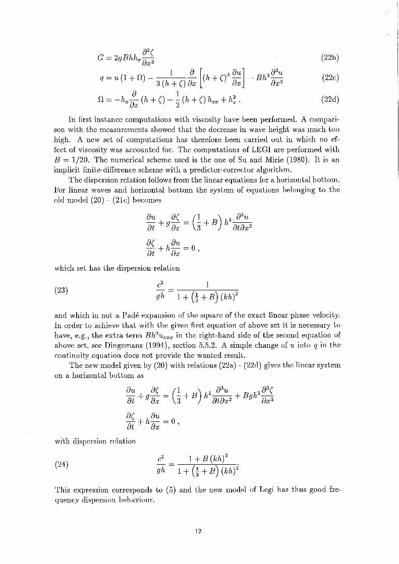
In first instance computations with viscosity have been performed. A compari­son with the measurements showed that the decrease in wave height was much too high. A new set of computations has therefore been carried out in which no ef­fect of viscosity was accounted for. The computations of LEGI are performed with B = 1/20. The numerical scheme used is the one of Su and Mirie (1980). I t is an implicit finite-difference scheme with a predictor-corrector algorithm.

The dispersion relation follows from the linear equations for a horizontal bottom. For linear waves and horizontal bottom the system of equations belonging to the old model (20) - (21c) becomes

du dc h'

d^u

dtdx'

which set has the dispersion relation

(23)

gh 1 + (I + 5 ) {khf

and which in not a Padé expansion of the square of the exact linear phase velocity. In order to achieve that with the given first equation of above set i t is necessary to have, e.g., the extra term Bh^u^xx in the right-hand side of the second equation of above set, see Dingemans (1994), section 5.5.2. A simple change of u into q in the continuity equation does not provide the wanted result.

The new model given by (20) with relations (22a) - (22d) gives the hnear system on a horizontal bottom as

du dC _ / I

~dt'^^di~ \ï

dt dx

+ B]h ' +Bgh'''^ dtdx' dx^

with dispersion relation

(24) 1 + B{khf

gh i+(l + B){khy

This expression corresponds to (5) and the new model of Legi has thus good fre­quency dispersion behaviour.

12

3.6. Snamprogetti (Snam). Broccliini of Snamprogetti performed computations with botli a Boussinesq-type model and a Serre-type model. The Boussinesq-type model is the same as given in (6) and the Serre-type model reads as follows.

du du ^ h' d^u dC d'u

dt + ""dx + ^dx ~ ""dxdt + 3 dx'dt + dx dxdt +

(25)

2 d^u h^d_

" 3 ^dx'dt 3 dx

2\

3.7. Technical University Delft ( T U D ) . The Boussinesq-like equations are derived from Madsen et al. (1991) and are written in terms of the averaged horizontal velocity, not in the fluxes. The equations have been published in Beji and Battjes (1994) an read

du du dC ( \ , \ , 2 , , 2 Ö ^ C

dt ' dx' "dx \3 ' J dx'dt ""dxdt dx^ (26)

dc^d_

dt dx {h + 0 u 0 .

We note that this set is not a reduction of the set (4) for small bottom slopes because the model is based on Madsen et al. (1991), not on the model with good shoaling behaviour (1) which has been proposed by Madsen et al. (1992). Essentially, Pere­grine's (1967) numerical scheme has been used, but the scheme for the continuity equation is different.

3.8. Other wave propagation models. For comparison purposes results of two more models are also incorporated in this note. Results of a Boundary Element model (Hypan), of Broeze (1993) and of a Hamiltonian model based on work of Radder (1992) and develloped in Otta and Dingemans (1994) are used also. Both of these models have exact linear frequency dispersion and the Boundary Element model gives one of the most accurate pre­dictions of non-linear wave motion which exists for non-breaking waves. The non-linearity in the Hamiltonian model as used here is of the same order as in the Boussinesq-like models. In principle also higher-order non-linearities may be in­cluded in the formulation, without unduly numerical difficulties, as i t seems now. For a mathematical description of the Hamiltonian model we refer to Radder (1992), Dingemans and Radder (1991) and Otta and Dingemans (1994).

4. Comparison of computations with measurements. With most of the numerical models discussed here computations for all three mea­surements have been provided. We give results of all models for test A, but give only a few results for tests B and C. I t turned out that test A was of such a discriminating nature that effectively the accuracy of all models could be judged from that case alone. The boundary condition at a; = 0 consists of a sinusoidal wave, with some slow start as needed by the different models. The slow start is not prescribed and

13

the free stirface profiles are taken long after the influence of the slow start has died out.

As the frequency dispersion proved to be of paramount importance, also for tests B and C results are shown for non-optimal frequency dispersion (i.e., 6 = 0) for both Boussinesq and Serre-type models. These results have been obtained with the D H I and Legi models.

4.1. Measurement condition A. A comparison between computations and measurements can be carried out in a number of ways. Whichever method is chosen, a graphical comparison is needed. Nearly all computations have been performed for a duration of 40 s, which is enough so that permanent wave profiles are obtained at the farthest stations. Over 23 m we have an average depth of 29.8 cm and thus, based on c = \/gh a mean celerity c = 1.71m/s so that i t takes 13.46 s for the main wave to travel the distance of 23 m. So much reserve is present that the free higher harmonics of interest have certainly reached the farthest station.

For test A we have T^Jgjh = 10.0, so the basic wave is well in the long wave

region (which may be loosely defined as Tsjgjh > 7). The test case A is such that on the horizontal bottom not much happens. This

has been checked by a computation with the Delft Hydraulics model (see Dingemans, 1994, section 5.9). Higher bound harmonic components are generated on the first slope and the shallow part is so short, while the local non-linearity is large, that not much phase difference between the free and the bound harmonics is developed here. On the second (downward) slope the depth increases rather fast and there the difference in celerity between the higher harmonic bound and free waves increases fast. I t is here where the difference between the various numerical models manifests itself clearly. The wave form changes much in this second slope region. This is clear from the measurements as given in Figure 3.

We plot all computed profiles ({xi,t) at the various stations Xi in the same way as the corresponding profiles of the measurements are plotted in Figure 3. By inspection of the computations with all models considered it follows that all models performed good upto the station at 13.5 m. Notice that this station lies on top of the bar (which extends from 12 to 14 m). That this good correspondence is true is shown on the two sets of equations of DHI , one with improved frequency dispersion (6 = 1/15) and one without i t (6 = 0).

In order to see in a more precise manner how weh the models behave, we plot of several models the profile at 19 and at 21 m directly over the measurement.

4.1.1. D H I results. Results with the D H I models for both improved frequency dispersion (6 = 1/15) and the usual case (6 = 0) have been given for all stations in Figure 8.

That the result of both computations is indeed the same up to 13.5 m, is shown in Figure 9 where the profiles have been plotted together. The correspondence between the computation and the measurement is shown in the right-hand part of Figure 9.

Beyond 13.5 m the results from both computations show markedly increasing differences. In order to facilitate the comparison with measurements, we plot all profiles for the computation and the measurement for a duration of about 4 s next

14

b = 0

b=1 /15

[ 1 / 1 ] c

0. 1 . 2 . 3, 4 . 5 . kh

FiG. 7. Deviations between computational and exact celerities.

28. 29. 30. 31. • 28. 29. 30. 31.

dhl , b = 0: -test A DHI. b=0: test A

F I G . 8. DHI, 6 = 0 (left)

dhl , b=1/15: test A DHI, b=1/15: test A

6 = 1 /15 (right), case A.

15

to each other. From these Figures i t becomes immediately clear wether a model per­forms good or not. For the DHI model with b = 1/15 i t is clear from Figure 10 that the computations and the measurements compare weh up to 17.3 m. This is stressed in Figures 11 and where the wave profiles of the computation and measurement at locations 15.7 m and 17.3 m have been plotted together.

At 21 m not such good correspondence of the computed and measured wave profile is found any more. This is also clear when the two profiles are plotted over each other, see Figure 13. This is also already clear at 19 m, see Figure 12.

In a Boussinesq-type wave propagation model the dispersion relation is necessar­ily approximated compared to the exact linear one. Even for a good approximation, eventually, after some distance, the (small) deviations between the phase velocities of the computational model and the exact linear one gives a cumulative effect in that the phases of the various free components differ much and the components even may become 180° out of phase. The distance over which this happens is much longer for an accurate approximation than for a less accurate approximation. But over large distances, when components have become free, the adagium that Boussinesq gives the correct profile at the wrong location remains true.

4.1.2. Delft Hydraulics and University of Groningen results. The results obtained with the Boussinesq programs of Delft Hydraulics and Univer­sity of Groningen are given in Figure 14 for the stations from 14.5 m onwards. In describing these results i t should be remembered that the University of Groningen model has a phase velocity which stems from a [1/1] Padé expansion of c', while the Delft Hydraulics model has a phase velocity which is equal to a [1/1] Padé expan­sion of c. The latter one is somewhat less accurate than the first one as is shown in Figures 6 and 7.

The results given in Figure 14 show that the University of Groningen model is more accurate than the Delft Hydraulics one. This can be explained from the more accurate dispersion relation of the Groningen model. The D H I result for b = 1/15 seems to be somewhat closer to the measurements than either of these two Boussinesq models based on a Hamiltonian approximation method. This is especially clear when considering the results for the station at 17.3 m

In Figure 15 a direct comparison with the measurement at location 21 m has been furnished.

4.1.3. Legi results. Legi results are available for the Serre-type model (20)-(22d) with two choices for the frequency-dispersion parameter: B = 0 and B = 1/20. Again only the results at the stations from 14.5 m onwards have been shown, see Figure 16. For B = 0 (not so good frequency dispersion) the computed wave profiles differ much with the measured ones, as has been noted before with other models with non-optimal frequency dispersion. For the case B = 1/20, as shown in the right-hand side of Figure 16, the correspondence with the measurements is better than has been obtained for other models with good frequency behaviour, i.e., the D H I model and the two Hamiltonian models (Delft Hydraulics and University of Groningen). This becomes especially clear from Figures 12 and 13.

The waves between 28 and 32 s are stable, i.e., all higher-harmonic components have reached the stations. This is shown in Figure 17 where the fu l l computation

16

DHI, b=1/15

DHI, b=0

DHI, b=1/15

13 .5 m 13 .5 m 1 [

ƒ \ ^

1 1 i 1 1 1 1 t

F I G . 9. Computations with DHI model Left: 6 = 0 and b = 1/15 at station 13.5 m for case A. Right: 6 = 1/15, with measurement at x = 13.5 m.

.0

-1 .5

.0 It

-1 .5

2.5 p

.0

-1 .5

2 ,5 p

.0

-1 .5

•WW

17.3 m 2.5 L i I . . i . . U 2.5

.0

-1 .5

.0

-1 ,5

I ' l l — I — I — I

_ l 1 1 I Ll

-1 ,5 J • • I L

38. 39, 40, 41,

WL meas, test A

28, 29, 30, 31,

DHI, b=0l test A

28, 29, 30. 31,

DHI, b=1/15: test A

F I G . 10. Measurements and DHI, 6 = 0, and 6 = 1/15, case A.

DHI, b=1/15 DHI, b=1/15

2,51 15,7 in 17 ,3 in

F I G . 11. Comparison DHI, 6 = 1/15, with measurement at x — 15.7 m, and at x = 17.3 m; case A.

17

DHI, b=1/15 Legi, b=1/20

F I G . 12 . Comparison DHI, h = 1 / 1 5 (left) and Legi (Serre, B=l/20) (right), with measure­ment at X = 19 m, case A.

DHI, b=l/15

29. \i 30. 31. \ 32 29. 30. 31. 32.

F I G . 13 . Comparison DHI, h = 1 / 1 5 (left) and Legi (Serre, B=l/20), with measurement at x 21 m, case A.

W ^ " f e ^ ' - few

14.5 n 14.5 m 14.5 n 2 .5 LA ' ' ' A ' ' U 2.5ri—

.0

-1 .5

.0

-1 .5

I S . 7 m -1—I—I—I—0 2.5

Z 3 19 m

2.5 L

I"' V ' ' V ' '"' - 1 .5 r ' ' ' ' ' ' ' "

38. 39. 40. 41.

WL meas. t e s t A

27. 28. 29. 30. UO (Hubs): teat A, bi r

' 27. 28. 29. 30. bqld, ino: test A, bin

F I G . 14. Results of University of Groningen (left), measurements (middle) and results of Delft Hydraulics (right), test A.

18

UG HL neas. meas.

21 O 21 «

2 .5 p 1 1 1 1 1 1 1 1 2 .5 n 1 1 1 I I I I—

FiG. 15 . Comparison of ihe Univ. of Groningen model (left) and the Delft Hydraulics model (right), with measurement at x = 21 m, case A.

Legi , b=0: test A L e g i , b=1/20: test A

F I G . 16 . Serre model of Legi: 5 = 0 (left), measurements (middle) and B = 1 / 2 0 (right), test A.

19

between 10 and 40 s has been shown for the stations from 14.5 m onwards. This case for Serre thus performs evidently better than the corresponding Bous­

sinesq case for improved frequency behaviour (i.e., the DHI result). This could be the case because although B = 1/20 is not a Padé expansion of the true linear phase velocity, the diiference of the resulting phase velocity with the exact linear one is smaller in the range 0 < kh < 3 (or, 0 < h/Xo < 1/2) than is obtained for the Padé expansion (h = 1/15).

4.1.4. Snamprogetti results. Snamprogetti furnished computations with both a Boussinesq model and a Serre-type model. The Boussinesq model is given by Eqs. (6) .In neither of the models an improved-frequency dispersion formulation has been used. The results have been shown in Figure 18. Because the frequency dispersion is not so good, the computed free surface profiles behind the bar do not conform well with the measurements. This is already clear from the profiles at 15.7 m, on the backward slope. Some difference between the Boussinesq and the Serre cases is found at the stations 21 and 23 m, but these differences are not large. I t is as if the Boussinesq case has different shoaling behaviour because all harmonics are more pronounced in the Boussinesq case than they are in the Serre case. The effect of the shoaling is already visible in the main peak at the station 14.5 m.

4.1.5. University of Thessaloniki results. Aristotle University of Technology (Karambas) furnished computations carried out with different models. One concerns computations with the usual Boussinesq-type model written in the vertically averaged velocity and the second one concerns a Boussinesq-type model with a kind of improved frequency dispersion. Of both mo­dels the wave profiles of the stations from 14.5 m onwards are plotted together with the measurements in Figure 21. As could have been expected, the model without frequency-dispersion improvement does not perform so good. The model with frequency dispersion improvement, (the right column in Figure 21) performs very well.

At 15.7 and 17.3m the correspondence with the measurements seems as good as the D H I model (see Figure 10), but at 19 m the D H I model performs slightly better, see Figures 12 and 19. Both models have essentially the same error at the latter station, which is most clearly seen in the trough of the waves. In the measurement a higher-harmonic is in anti-phase with the basic wave, but in both computations that higher harmonic seems to be in phase with the basic wave. At 21 m the AUT model performs better than the D H I model. See Figure 19.

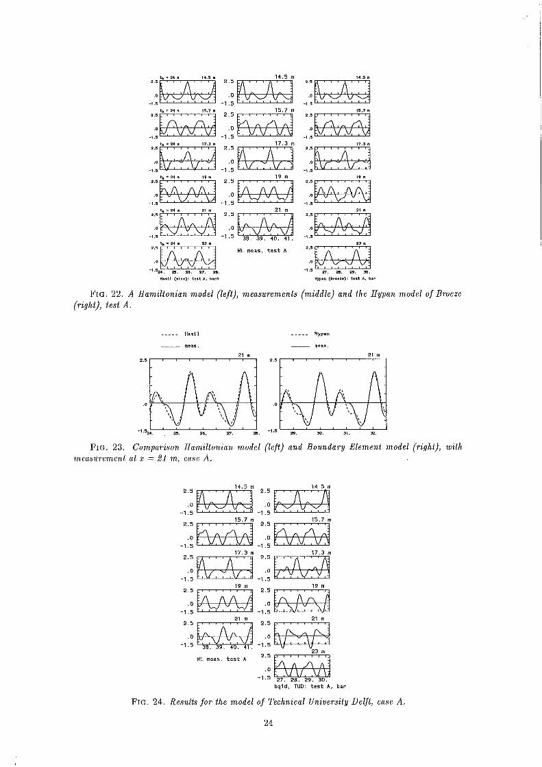
4.1.6. A Hamiltonian and a Boundary Element model. A Hamiltonian model for waves in which the long-wave assumption has not been made, has been proposed by Radder (1992). A description of the model and its numerical evaluation in two ways^ is given in Otta and Dingemans (1994). Results from the time-domain model are given in Figure 22, again for stations from 14.5 m onwards. The form as used here is of Boussinesq-type of approximation with respect to the non-linearity but has exact linear dispersion relation. (In the limit for

^ One of the models is the solution of the time-evolution equations. The other one consists of an expansion in terms of sine functions. Results of the second one are given here.

20

.0

-1 .5

2.5

.0

-1 .5

2 .5 F

.0

-1 .5

2.5

.0

-1 .5

F I G . 17 . Serre model of Legi: B = 1 /20 . time-window from 10 to 40 s. Test A.

14.5 m

15.7 m

17.3 m

26. 27. 28. 29. Snam, Serre: t e s t A, bar

16. 27. 28. 29. Snam, Boussinesq: t e s t A, bar

F I G . 18 . Snamprogetti: Serre (left), measurements (middle) and Boussinesq (right), test A.

Snara, Serre

27. 28 25. 26 , 27 . 28.

F I G . 19 . Comparison AUT model (left) and Snamprogetti Serre model (right), with measure­ment at X = 19 m, case A.

21

Aut, F Snail, Serre

AUT, test A, bar AUT, test At, bar

FiG. 21. AUT; model (11) (left), measurements (middle) and Boussinesq (right), test A.

22

vanisliiiig amplitude the model is the usual linear wave propagation model.) Higher-order approximations with respect to the non-linearity are possible but are not used here. These higher-order non-linearities are short-wave non-linearities. These are of importance, amongst others, in accurate modelling of solitary waves where steep gradients occur.

Because boundary-element models can give an accurate description of the free surface elevation, also a computation has been performed by Broeze with the model Hypan as dexcribed by Broeze (1993). These results are also shown in Figure 22.

I t is seen that up to 17.3 m an excehent correspondece with the measurements is found. Also at 21 m a good correspondence is found, especially for the boundary element model, see Figure 23. The Hamiltonian model performs slightly less as can be seen in Figure 23. This is ascribed to the neglect of the short-wave non-linearities. Notice that the small depression in the crest of the measured free surface profile at 15.7 m is only predicted by the boundary element model. A l l other computations miss this feature.

At 17.3 m the two peaks in the computed free surface profile are almost equal, as in the measurement, but the phases of the short waves are different. Again i t is seen that in the boundary element model more short wave behaviour is visible than in the Hamiltonian model. This is typically due to a better modelhng of the non-linearities. We notice that also with Boussinesq (e.g., the D H I model with b = 1/15), the correspondence at 19 m was less than the correspondence at 21 m. Possibly this is due to the place in the wave profile where the higher harmonics manifest themselves. When they are visible in the trough a small deviation looks much more significant than when the same deviation occurs elsewhere in the profile.

We conclude that the correspondence between the free surface profiles of the boundary element computation and the measurements is excehent. The Hamiltonian model performs slightly less, but is still slightly better than any of the Boussinesq-type or Serre-type models. This is to be expected because of the correct frequency dispersion in the model.

4.1.7. Results of Technical University Delft. Results for case A have been given in Figure 24.

The results are seen to be similar to those of DHI , but are not exactly the same. Variations are visible in the Figures. At 15.7 TUD's result seems better, but at 19 m we see the same phase difference in comparison to the measurements as in the D H I case.

4.2. Measurement condition B . Results of all models have been shown for measuring condition A. For measuring conditions B and C we now only show results obtained with Boussinesq and Serre models which gave good results for measuring condition A. We now have a longer wave than in case A, which is also evident from the value of the shallowness pa­rameter Tsjgjh = 12.5. The effect of a longer basic wave is that the generation of higher-harmonics develops stronger (the phase mismatch is smaller and therefore the interaction time that waves may effectively interact with each other is longer). Stronger interaction also means that still higher harmonics may be generated.

We show the results obtained with the Boussinesq model of D H I and the Serre model of Legi. In order to show that a good dispersion relation remains important

23

2.5

-1.5

2.5

.0

-1.5

2.5

.0

2.5

.0

-1.5

2.3

.0

-1.5

2.5

.0

P X 14.5 n

J 2 . 5

-1 .5

2.5

-1 .5

2 .5

.0

-1 .5

2.5

.0

2 .S

.0

-1 .5

l ' t ,3 r - A ' ' ' A ' ' '

a.5

-1.5

1

2.5

.0

R 2.5

.0

-1.5

2.5

.0

2.5

.0

-1.5

c 1

X t.5 n

2.5

-1.5

2.5

.0

-1.5

2.5

.0

2.5

.0

-1.5

2.3

.0

-1.5

2.5

.0

tfc = 24 1 15.7 a

2 . 5

-1 .5

2.5

-1 .5

2 .5

.0

-1 .5

2.5

.0

2 .S

.0

-1 .5

15.7 r

a.5

-1.5

1

2.5

.0

R 2.5

.0

-1.5

2.5

.0

2.5

.0

-1.5

-1 1 1 1 1 1

1 5.7 n

2.5

-1.5

2.5

.0

-1.5

2.5

.0

2.5

.0

-1.5

2.3

.0

-1.5

2.5

.0

2 . 5

-1 .5

2.5

-1 .5

2 .5

.0

-1 .5

2.5

.0

2 .S

.0

-1 .5

1 1 r 1 1 1 r r

a.5

-1.5

1

2.5

.0

R 2.5

.0

-1.5

2.5

.0

2.5

.0

-1.5

2.5

-1.5

2.5

.0

-1.5

2.5

.0

2.5

.0

-1.5

2.3

.0

-1.5

2.5

.0

t| » 24 V y. a

V • 17.3 n

2 . 5

-1 .5

2.5

-1 .5

2 .5

.0

-1 .5

2.5

.0

2 .S

.0

-1 .5

• , V , V , V , \3 17.3 r

a.5

-1.5

1

2.5

.0

R 2.5

.0

-1.5

2.5

.0

2.5

.0

-1.5

V .V.

1

V 7.3 n

2.5

-1.5

2.5

.0

-1.5

2.5

.0

2.5

.0

-1.5

2.3

.0

-1.5

2.5

.0

W-

2 . 5

-1 .5

2.5

-1 .5

2 .5

.0

-1 .5

2.5

.0

2 .S

.0

-1 .5

J > > I 1 I • l

a.5

-1.5

1

2.5

.0

R 2.5

.0

-1.5

2.5

.0

2.5

.0

-1.5

2.5

-1.5

2.5

.0

-1.5

2.5

.0

2.5

.0

-1.5

2.3

.0

-1.5

2.5

.0

tfc = 24

. . V s 19 n

2 . 5

-1 .5

2.5

-1 .5

2 .5

.0

-1 .5

2.5

.0

2 .S

.0

-1 .5

•. v/ , . . \ / . .¬19 m

a.5

-1.5

1

2.5

.0

R 2.5

.0

-1.5

2.5

.0

2.5

.0

-1.5

1 l \ /

1 9 n

2.5

-1.5

2.5

.0

-1.5

2.5

.0

2.5

.0

-1.5

2.3

.0

-1.5

2.5

.0

1

2 . 5

-1 .5

2.5

-1 .5

2 .5

.0

-1 .5

2.5

.0

2 .S

.0

-1 .5

l l l l l l l l

a.5

-1.5

1

2.5

.0

R 2.5

.0

-1.5

2.5

.0

2.5

.0

-1.5

2.5

-1.5

2.5

.0

-1.5

2.5

.0

2.5

.0

-1.5

2.3

.0

-1.5

2.5

.0

t, . 24 a

V i 21 n

2 . 5

-1 .5

2.5

-1 .5

2 .5

.0

-1 .5

2.5

.0

2 .S

.0

-1 .5

1 1 1 1 1 1 1 L

21 m

a.5

-1.5

1

2.5

.0

R 2.5

.0

-1.5

2.5

.0

2.5

.0

-1.5

J 1 L -

2

V n

2.5

-1.5

2.5

.0

-1.5

2.5

.0

2.5

.0

-1.5

2.3

.0

-1.5

2.5

.0

: /, V

2 . 5

-1 .5

2.5

-1 .5

2 .5

.0

-1 .5

2.5

.0

2 .S

.0

-1 .5

« U W

a.5

-1.5

1

2.5

.0

R 2.5

.0

-1.5

2.5

.0

2.5

.0

-1.5

[-/•l...

2.5

-1.5

2.5

.0

-1.5

2.5

.0

2.5

.0

-1.5

2.3

.0

-1.5

2.5

.0

i, = 24 9

r 1

23 n

2 . 5

-1 .5

2.5

-1 .5

2 .5

.0

-1 .5

2.5

.0

2 .S

.0

-1 .5 - . . V . . . V r

3 8 . 3 9 . 40. 41

a.5

-1.5

1

2.5

.0

R 2.5

.0

-1.5

2.5

.0

2.5

.0

-1.5 ri 1 1

2 3 H

2.5

-1.5

2.5

.0

-1.5

2.5

.0

2.5

.0

-1.5

2.3

.0

-1.5

2.5

.0

- / \ 1

V 1

WL meas, t e s t A

.0 uv l 1 1

Hin l l (alno); test A, bir3 H/pin (Broeze)! tesl

FiG. 22. ^ Hamiltonian model (left), measurements (middle) and the Hypan model of Broeze (right), test A.

Hypan

29 , 30, 31, 32,

F I G . 23. Comparison Hamiltonian model (left) and Boundary Element model (right), with measurement at x = 21 m, case A.

.0 - 1 . S

17,3 m ^ ^

,0

-1,5

19 ffl

WL meas, t e s t A

,0

-1 ,5

17.3 m

27, 23, 29, 30, bqld, TUD: tes t A, bar

F I G . 24. Results for the model of Technical University Delft, case A.

24

also for test cases B and C, results with both b = 0 and b = 1/15 are shown for D H I (Figure 25) and results for both 6 = 0 and 6 = 1/20 are shown for Legi (Figure 26).

Consider the right-hand column of Figure 25. A good correspondence is obtained at the station at 14.5 m. At 15.7 m the correspondence between computation and measurement is much less. In the measurement we have two peaks of approximately equal height between two very small peaks. In the computation these two peaks are of unequal height. The correspondence at 17.3 and 19 m seems to be better than that at 15.7 m.

The Techn. Univ. Delft model and the Delft Hydraulics one do not perform so good for case B, see Fig. 28. For Delft Hydraulics, see also the comparison at 19 m as given in Figure 27.

4.3. Measurement condition C . For measuring condition C we show the results of D H I for both 6 = 0 and 6 = 1/15 (Figure 29) and the ones of the Serre model of Legi with 6 = 0 and 6 = 1/20 (Figure 30). For this condition we have T^g/h, = 5.0 in the deep part, so we have a rather short basic wave. Whereas the measured free surface profiles are tilted first to the right, and later to the left, the computed profiles, especially from 15.7 m onwards are very symmetrical with respect to the vertical. I t is as if the computations are not able to generate enough second and third harmonic amplitude. As for the generation of higher harmonics a small phase mismatch (i.e., AA; — k2 — 2fci) is permitted, the mismatch grows rapidly for shorter waves, and, moreover the error between the mismatch as experienced in the Boussinesq model and the one in the measurements also grows. Therefore, in the measurements a smaller mismatch would be present with as effect more higher-harmonic consituents in the signal.

From inspection of Figures 29 and 30 i t is evident that the wave profiles are too symmetrical. To show how far off i t is, one of the profiles, at 19 m, is compared directly with the measured profile, see Figure 32. From that Figure i t is clear that the skewness of the computed profiles i t too low, but the correrspondence is not that bad either. To test i f the reason for the symmetry in profile is indeed the larger mismatch, also the result obtained with the Boussinesq model of Delft Hydraulics is considered. From the results of these computations, given in Figure 31, a much closer correspondence in skewness is seen, see also Figure 32. Here the Delft Hydraulics profile evidently performs best. Because on basis of physical arguments i t can be argued that the D H I Boussinesq model should perform better than the Delft Hydraulics one, a different reason for this behaviour should be found. We now look into some numerics. Many numerical schemes do have some effect of numerical diffusion. When adding a diffusion term to the momentum equation, resulting wave profiles are typically more symmetric than the corresponding measured profile.

The computational procedure followed in the Delft Hydraulics Boussinesq model is based on a method of lines in space and the resulting ordinary differential equations in time are solved with a fourth-order Runge-Kutta integration method. As for case C we have A t = 0.02525 s and Aa; = 0.05 m and y/gh = 1.981 m/s at 40 cm depth,

25

4.0 14.5 m

I I I I .1 I I 4.0 14.5 m

}J\A.J\A .0 J\j\J\/\:

21 m 21 m

2.5 ' ' ' I ' ' I ' ' 1 -2 .5 45. 46. 47. 48. 49.

28. 29. 30. 31 . 32

DHI, b=0; test B

28. 29. 30. 31 . 32.

DHI, b=1/15: test 8

F I G . 25. f iTJ, Results forb = 0 (left) and h = 1/15 (right), and measurements (middle), case B; stations from 14-5 m onwards.

0 , i'';=> ^ Q 14.5 m ^ ^ 14.5

°|\/U71AJ .01JUJl/j .°?l/vJl/vJ

.0

-2 .5

15.7 m I I I I I i | 4.0

45. 45. 47. 48. 49. "^'^

35. 36. 37. 38. 39. 40.

Leg i , b=0l test B

35. 35. 37. 38. 39. 40.

L e g i , b=1/20; test B

F I G . 26. Legi, Results of the Serre model with 5 = 0 (left) and B = 1/20 (right), and measurements (middle), case B; stations from 14-5 m onwards.

DHI, b=1/15 Legi, b=1/20 WL

meas.

29. 30 29. 30, 28. 29. 30. 31.

F I G . 27. Comparison DHI, h = 1/15 (left) Legi (Serre, B=l/20) (middle) and Delft Hydraulics (Boussinesq) (right), with measurement at x = 19 m, case B.

26

we have the CFL number^

CFL = x f g h ^ = 1.00 . ^ Aa;

Recently Petit (1994) considered the dissipation for a hyperbolic equation of the form Ut + cux = 0 for a number of integration schemes as a function of fcAa;, with k the wave number ( = 2 7 r / A ) . For fourth-order central-space Runge-Kutta discretisations and CFL < 2^/2 for stability, the growth factor D of the amplitudes of wave-like solutions is given in Figure 33. As kAx = 0.21 we are in the region A;Aa; < 0.3 and virtually no dissipation (Z) = 1) is present in the scheme. A reason of the better behaviour of the Delft Hydraulics Boussinesq model for case C could be contained in the numerical procedure followed.

The result from both the Boussinesq-type model of D H I and the Serre-type model of Legi, both with improved freqency dispersion, is rather disappointing in case of the short-wave test C. For the Legi model without frequency dispersion improvement the results at 21 and 23 m are strange. This needs further attention. We therefore plot all the computational data beyond 10 s, see Figure 34. For B = 0, the computation time is shorter than for the case B = 1/20 due to the development of instabilitites. In fact 40 s is needed.

The Techn. Univ. of Delft result for test C, as given in Figure 31, seems to be not as good as tha one of Delft Hydraulics. At 15.7 Techn. Univ. Delft is better, but at 17.3 and 19 Delft Hydraulics is much better. The result of Techn. Univ. Delft shows more variation in wave form than the one of DHI , notwithstanding the fact that both models are almost the same in formulation.

5. Discussion and recommendations. We see that i t is important that the free harmonics have an accurate phase velocity. The frequency-dispersion modelling is much more important than the modelhng for possible higher waves. Thus the competition between Serre-type and Boussinesq-type models is usually won by the one with best frequency dispersion characteristics. That is, the linear properties are the most important ones for good correspondence with measurements. Of course, that does not mean that no modelling of non-linearity is necessary, because the non-linearity is the source of the generation of higher harmonics, and these higher harmonics, when they get free, have their own phase velocity. In (fairly) long-wave approximations the attention is usually focussed to the basic wave to be long enough, but also the third or fourth harmonic should have a wave length which is long enough.

For models with the same frequency behaviour the differences are in the mod­elling of the non-linearity and the modelling of the slope-dependent terms. For small slopes, Madsen et al. (1992) have shown that small differences in the depth-dependent terms may give large differences in the linear shoaling characteristics. A number of examples with widely different shoaling characteristics have been dis­cussed also by Dingemans (1994).

The Boussinesq-type and Serre-type models of DHI and Legi-IMG do not per­form so well for test C (At least, cases A and B mede one expect better behaviour for case C as weh). The Boussinesq model of Delft Hydraulics performs better for

^ For case B we have the same parameters and for case A are used Aa; = 0.05 m and At = 0.05 s, resulting in CFL = 1.98.

27

27.>S8. 29. 3 » . 31 . bqld, wlb: t e s t B, bar

FiG. 28 . Technical Univ. Delft (left), measurements (middle), and Delft Hydraulics, Boussi­nesq (right), case B.

4.0

.0 -2.0

4.0

.0 -2,0

4.0

-2.0

4.0

-2.0

4.0

-2.0

4.0

.0 -2.0

14.5 " 4,0

-2,0

" 4,0

,0 -2 ,0

n

4,0

-2 ,0

4,0

,0 -2,0

4,0

-2 ,0

14,5 m

4.0

.0

-a .o

m 4.0

.0

-2 .0

m

14.5 • 4.0

.0 -2.0

4.0

.0 -2,0

4.0

-2.0

4.0

-2.0

4.0

-2.0

4.0

.0 -2.0

15,7

" 4,0

-2,0

" 4,0

,0 -2 ,0

n

4,0

-2 ,0

4,0

,0 -2,0

4,0

-2 ,0

15,7

m

4.0

.0

-a .o

m 4.0

.0

-2 .0

m

A \A A / A tS .7 •

4.0

.0 -2.0

4.0

.0 -2,0

4.0

-2.0

4.0

-2.0

4.0

-2.0

4.0

.0 -2.0

\ / \ A J -

" 4,0

-2,0

" 4,0

,0 -2 ,0

n

4,0

-2 ,0

4,0

,0 -2,0

4,0

-2 ,0

1 1 1 1 1 1

m

4.0

.0

-a .o

m 4.0

.0

-2 .0

m

-T 1 1 1 1 (—

4.0

.0 -2.0

4.0

.0 -2,0

4.0

-2.0

4.0

-2.0

4.0

-2.0

4.0

.0 -2.0

17.3

" 4,0

-2,0

" 4,0

,0 -2 ,0

n

4,0

-2 ,0

4,0

,0 -2,0

4,0

-2 ,0

i V y , ,\y, ,\y,

17,3

m

4.0

.0

-a .o

m 4.0

.0

-2 .0

m 17.3 •

4.0

.0 -2.0

4.0

.0 -2,0

4.0

-2.0

4.0

-2.0

4.0

-2.0

4.0

.0 -2.0

\ A A J

" 4,0

-2,0

" 4,0

,0 -2 ,0

n

4,0

-2 ,0

4,0

,0 -2,0

4,0

-2 ,0

4.0

• •A A A

4.0

.0 -2.0

4.0

.0 -2,0

4.0

-2.0

4.0

-2.0

4.0

-2.0

4.0

.0 -2.0

19 m

" 4,0

-2,0

" 4,0

,0 -2 ,0

n

4,0

-2 ,0

4,0

,0 -2,0

4,0

-2 ,0

19 m

4.0

• :/ A./ A y 19 s

4.0

.0 -2.0

4.0

.0 -2,0

4.0

-2.0

4.0

-2.0

4.0

-2.0

4.0

.0 -2.0

A A A

" 4,0

-2,0

" 4,0

,0 -2 ,0

n

4,0

-2 ,0

4,0

,0 -2,0

4,0

-2 ,0

4.0

.0

-a .o

4.0

-2 .0

-1 1 1 1 1 1—

A A

4.0

.0 -2.0

4.0

.0 -2,0

4.0

-2.0

4.0

-2.0

4.0

-2.0

4.0

.0 -2.0

'. \ / . \ / . .V 21 m

" 4,0

-2,0

" 4,0

,0 -2 ,0

n

4,0

-2 ,0

4,0

,0 -2,0

4,0

-2 ,0

7 • \ / • V / , S

21 m

4.0

.0

-a .o

4.0

-2 .0

S l •

4.0

.0 -2.0

4.0

.0 -2,0

4.0

-2.0

4.0

-2.0

4.0

-2.0

4.0

.0 -2.0

" 4,0

-2,0

" 4,0

,0 -2 ,0

n

4,0

-2 ,0

4,0

,0 -2,0

4,0

-2 ,0

1 1 1 1 1 1

4.0

.0

-a .o

4.0

-2 .0

k A A /

4.0

.0 -2.0

4.0

.0 -2,0

4.0

-2.0

4.0

-2.0

4.0

-2.0

4.0

.0 -2.0

\ / , K / , K / ,

23 m

" 4,0

-2,0

" 4,0

,0 -2 ,0

n

4,0

-2 ,0

4,0

,0 -2,0

4,0

-2 ,0

1 - I t^ 1 • L

38. 39. 40.

4.0

.0

-a .o

4.0

-2 .0 •A / A / A / -S3 •

4.0

.0 -2.0

4.0

.0 -2,0

4.0

-2.0

4.0

-2.0

4.0

-2.0

4.0

.0 -2.0

WL meas, tes t 0, bar '

,0

- s , o

-1 1 1 1 1 1—

4.0

.0 -2.0

4.0

.0 -2,0

4.0

-2.0

4.0

-2.0

4.0

-2.0

4.0

.0 -2.0 r V 1 V 1 \ /

28. 29, 30,

)HI, b=0: test C

WL meas, tes t 0, bar '

,0

- s , o Ll

SB. a9. 30.

)HI, b-1/15: Umi C

F I G . 29 . DHI, Results forb=Q (left) and b = 1 / 15 (right), and measurements (middle), case C; stations from 14-5 m onwards.

28

14.5 m

28. 29. 30

Leg i , b=0l test 0 Leg i , b=1/20: test 0

F i G . 30. Legi, Results ihe Serre model with 5 = 0 (left) and B = 1/20 (right), and measure­ments (middle); stations from 14-5 m onwards, case C.

27. 28. 29. 30. bqld, wlc: t e s t C, bar

F I G . 31. Techn. Univ. Delft (left), measurements (middle) and Delft Hydraulics, Boussinesq (righi), case C.

DHI, b=1/15 Legi, b=1/20

meas.

WL

reeas.

2 8 . 29 . 30 . 31 . •"' 32 . 33 . M. 3 5 . " ^ ' ° 2 8 . 2 9 . 30 .

F I G . 32 . Comparison of DHI (left) Legi (middle) and Delft Hydraulics Boussinesq model (right) with measurement at x = 19 m, case C.

29

1.0 2.0 3.0

kAx

F I G . 33. Growth factor D for amplitude for a fourth-order Runge-Kutta central space scheme. Here n is the CFL parameter.

.0 I-^WVAAAAAA/I

15.7 m

21 m

10. 15. 20.

Legi , 8 = 0, t.!xt C

25. 30.

.0 Ï-VAAAAA/I 15.7 m

.0 -2.0

.0 -2.0

.0 -2.0

4.0

.0 -2.0

.0 -2.0

21 m

23 m

10, 15. 20. 25.

Legi , B = 1/20, text C

30. 35. 40.

F I G . 34. Serre model of Legi. Test C: left B - Q and right B = 1/20. time-window from 10 to 40 s.

30