massively parallel approximation of irregular triangular meshes of arbitrary topology with smooth...
TRANSCRIPT

Theoretical Computer Science
ELSEVIER Theoretical Computer Science 162 (1996) 35 I-369
Massively parallel approximation of irregular triangular meshes of arbitrary topology
with smooth parametric surfaces
Miguel Angel Garcia*
Diaision of Robotics and Artificial Intelligence, Institute of ~vbernrtics,
PoJl,terhnic Uniwrsiv of Catuloniu, Diagonal 647. planta 2. OK028 Barcrlona, Spain
Abstract
This paper describes a parallel implementation of a previously developed mathematical model intended for the approximation of 3D triangular meshes with smooth surfaces yielding
first order geometric continuity G’. This represents a novel application of SIMD architectures to the approximation of irregular meshes. Previous related works have focused on the approxi- mation of rectangular meshes using tensor-product approximants, such as B-splines, that suit the regular structure of most parallel architectures.
A parallel implementation of the proposed surface model at three degrees of granularity shows that a coarse grain scheme yields maximum performance when each control triangle is
approximated by a single processor avoiding inter-processor communication. The data distri- bution necessary to attain an independent task-farm topology is studied. The different algo- rithms have been implemented using a data-parallel model and tested on two Connection Machine 200 parallel computers with 4 and 16 K processors, respectively. The algorithms achieve efficiencies close to a 100% and scale linearly in the number of processors.
Keywords: Geometric modeling; Surface approximation; Triangular meshes;
Data-parallelism; Connection machine
1. Introduction
The reconstruction of surfaces defined by irregular triangular meshes of 3D control
points is a problem found in a wide variety of disciplines. Triangular meshes are an
effective way of storing geometric information describing the shape of objects of
arbitrary complexity. Their scattered nature enables the representation of surfaces at
multiple resolutions, concentrating points in rapidly changing areas and dispersing
* Fax: + 34 3 401 66 05; e-mail: [email protected]
0304-3975/96/$15.00 c 1996-Elsevier Science B.V. All rights reserved SSDI 0304-3975(95)00037-O
352 MA. Garcia 1 Theoretical Computer Science 162 (1996) 351-369
them in regions of little variation. Moreover, since those meshes are based on very
simple primitives (triangles), many geometric algorithms (collision detection, for
example) may be simplified considerably. Therefore, triangular meshes are widely
used to represent either synthetically or sensorially generated object surfaces in fields
such as computer graphics, geographic information systems (GIS) or robotics. Conse-
quently, the availability of techniques for estimating the original surfaces represented
by such triangular meshes is of great interest to all those fields.
On the other hand, the task of surface reconstruction is frequently associated with
tight timing constraints due to real-time requirements of many of the applications that
demand this kind of processes. Virtual reality or robot navigation are typical exam-
ples. In order to satisfy those constraints, the utilization of parallel computers is likely
to be beneficial.
The problem of generating smooth surfaces through interpolation or approxima-
tion of control meshes of arbitrary topology does not fit the regular structure of most
parallel architectures. If the structure of the control mesh does not coincide with the
structure of the computer’s interconnection network, the parallel process must rely on
irregular patterns of communication that lead to significant time penalties. Thus, it is
not surprising that previous related research [l, 7,9,12] has focused on the problem of
parallel generation of tensor-product splines, such as Bezier or B-splines, since they
approximate or interpolate surfaces defined by rectangular meshes of control points.
Unfortunately, rectangular meshes cannot represent surfaces of arbitrary topology
directly. The author is unaware of previous work regarding the parallel approxima-
tion or interpolation of nonrectangular meshes with smooth surfaces.
This paper presents a novel application of SIMD architectures to the problem of
approximation of irregular triangular meshes of control points. A parallel implemen-
tation of a geometric model previously developed by the author is described. This
model was originally proposed as a graphics tool [2] for approximating triangular
meshes of control points with smooth parametric surfaces. Later on, the model was
proposed as an efficient tool for surface reconstruction through geometric fusion of
neighborhoods of noisy points obtained by sensing [3]. A further extension [4]
included interpolation capabilities and was applied to the reconstruction of terrain
surfaces in GIS allowing for uncertainty. The model fulfills a set of valuable properties
[S] that make it suitable for the efficient representation of complex surfaces of
arbitrary topology and genus.
Every surface generated with this technique is composed of as many triangular
surface patches as triangles in its associated control mesh. Each patch is generated by
a parametric function that approximates the 3D positions of the control points of
a triangle. Two parametric functions, S &P) and GAB,-(P), are defined. The first
function generates triangular surface patches that join with function continuity (Co
continuity). Hence, adjacent patches share the same boundary curves and, therefore,
there are no steps between them. The second parametric function generates triangular
surface patches that join with first-order geometric continuity (G’ continuity). This
means that adjacent patches join with the same tangent plane along their common
MA. Garcia J Theoretical Computer Science 162 (1996) 351-369 353
boundary curves. GA&P) is directly obtained from S,,,(P) by modifying the three
borders of the latter with cubic Bezier curves calculated to yield the desired continuity.
In a preliminary work [6], three parallel implementations of S,,,(P) were analyzed
considering different levels of granularity. The programs were tested on a data-
parallel system, the Connection-Machine CM-200. This computer was chosen since it
supports a collection of high-level languages, such as C*, that allow the definition of
parallel algorithms in vector notation directly, with independence of the underlying
architecture. A coarse granularity implementation, in which each surface patch is
generated on a single processor, produced the best results when no communication
among processors occurred. Efficiencies close to 100% were obtained.
This paper presents a parallel implementation at coarse granularity of the whole
geometric model, including the GAB&‘) functions. The data distribution among
processors in order to attain an independent task-farm topology that guarantees
maximum efficiency is also analyzed and experimental results are given. The next
section summarizes the geometric model. Section 3 describes the parallel algorithm.
Section 4 gives experimental results of this technique on two CM-200 systems of 4 and
16 K processors. Finally, conclusions are given and future lines suggested in Section 5.
2. Geometric approximation of triangular meshes
The aim of this work is the generation of a smooth surface that approximates the
3D control points of a given triangular mesh of arbitrary topology.
A triangular mesh d is defined as the set LI = {CP, T), where CP is a set of 3D
control points and T is a description of the mesh topology as a valid triangulation of
those points. Each control point X is defined by three spatial coordinates and
a weighting factor: X = {(x,, y,, zx), Wx>. The weighting factor Wx represents the
attraction exerted by that point upon the surface. The mesh topology is represented as
a set of polygonal patches associated with each control point. A polygonal patch
associated with a point X lists the identifiers of the control points adjacent to X in
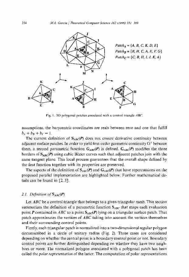
counterclockwise order. According to this definition, every control triangle is asso-
ciated with three polygonal patches. For instance, Fig. 1 shows the three polygonal
patches associated with a control triangle ABC. Polygonal patches may be interpreted
as irregular polygons in space.
Each control triangle, in general denoted as ABC, is the definition domain of
a parametric surface patch S,,,(P) that approximates the three vertices of ABC. This
approximation takes into account all the control points that belong to the three
polygonal patches that contain ABC. The parameter P represents the position inside
ABC where the function is evaluated. P is referred to as the evaluation point. The
evaluation point is represented by its barycentric coordinates with respect to the
vertices of ABC. The barycentric coordinates (bA, b,, bc) of a point P contained in
a triangle ABC are the coefficients of the expression P = b,A + bgB + b,C, where
A, B and C are the 3D coordinates of the control points that define ABC. Under these
354 MA. Garcia / Theoretical Computer Science 162 (1996) 351-369
Patch* = (A, B, C, K, D, E)
PatchB = {B, H, C, A, E, I;: G)
Patchc = { C, B, H, I, J, K, A}
K + J
I H
D H
E G B F
Fig. 1. 3D polygonal patches associated with a control triangle ABC.
assumptions, the barycentric coordinates are reals between zero and one that fulfill
bA+bs+bc=l.
The current definition of S,,,(P) does not ensure derivative continuity between
adjacent surface patches. In order to yield first-order geometric continuity G’ between
them, a second parametric function G ,&P) is defined. G&P) modifies the three
borders of S,,,(P) using cubic Bezier curves such that adjacent patches join with the
same tangent plane. This local process guarantees that the overall shape defined by
the first function together with its properties are preserved.
The aspects of the definition of S,,,(P) and GA&‘) that have repercussions on the
proposed parallel implementation are highlighted below. Further mathematical de-
tails can be found in [2, 31.
2.1. Dejnition of SAB,-(P)
Let ABC be a control triangle that belongs to a given triangular mesh. This section
summarizes the definition of a parametric function S,,c that maps each evaluation
point P contained in ABC to a point SABc(P) lying on a triangular surface patch. That
patch approximates the vertices of ABC taking into account the vertices themselves
and their surrounding control points.
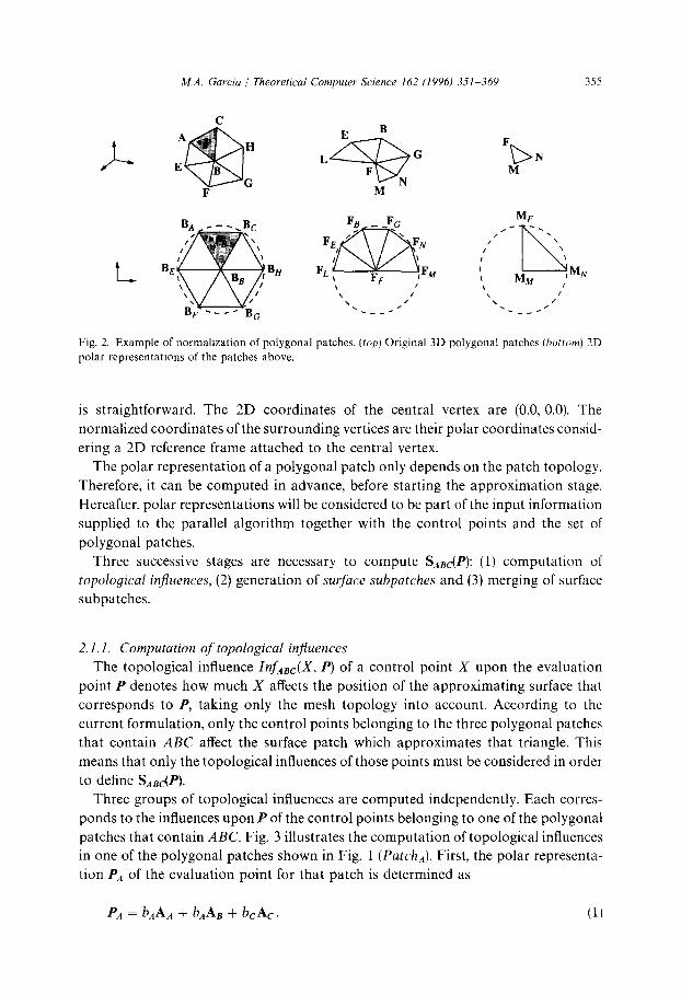
Firstly, each triangular patch is normalized into a two-dimensional regular polygon
circumscribed in a circle of unitary radius (Fig. 2). Three cases are considered
depending on whether the central point is a boundary control point or not. Boundary
control points are further distinguished depending on whether they have two neigh-
bors or more. The normalized polygon associated with a polygonal patch has been
called the polar representation of the latter. The computation of polar representations
M.A. Garcia / Theoretical Computer Science 162 (1996) 351-369 355
t BE
Fig. 2. Example of normalization of polygonal patches. (top) Original 3D polygonal patches (hotrom) 2D
polar representations of the patches above.
is straightforward. The 2D coordinates of the central vertex are (0.0, 0.0). The
normalized coordinates of the surrounding vertices are their polar coordinates consid-
ering a 2D reference frame attached to the central vertex.
The polar representation of a polygonal patch only depends on the patch topology.
Therefore, it can be computed in advance, before starting the approximation stage.
Hereafter, polar representations will be considered to be part of the input information
supplied to the parallel algorithm together with the control points and the set of
polygonal patches.
Three successive stages are necessary to compute S,,,(P): (1) computation of
topological injuences, (2) generation of surface subpatches and (3) merging of surface
subpatches.
2.1. I. Computution of topological in&em-es
The topological influence ZnfABc(X, P) of a control point X upon the evaluation
point P denotes how much X affects the position of the approximating surface that
corresponds to P, taking only the mesh topology into account. According to the
current formulation, only the control points belonging to the three polygonal patches
that contain ABC affect the surface patch which approximates that triangle. This
means that only the topological influences of those points must be considered in order
to define S,,,(P). Three groups of topological influences are computed independently. Each corres-
ponds to the influences upon P of the control points belonging to one of the polygonal.
patches that contain ABC. Fig. 3 illustrates the computation of topological influences
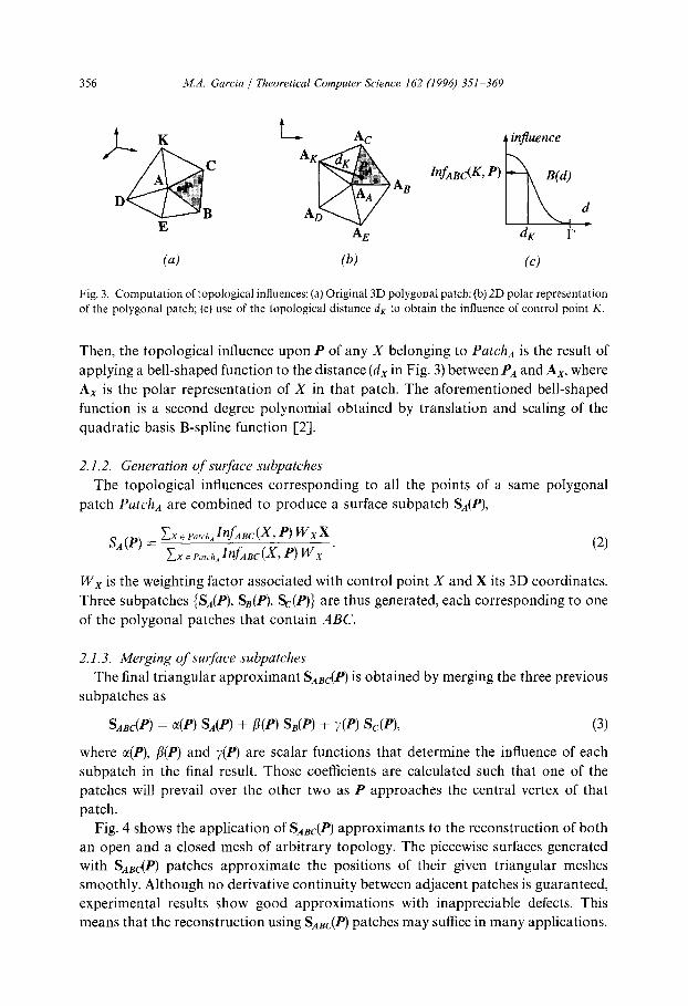
in one of the polygonal patches shown in Fig. 1 (Pat&J. First, the polar representa-
tion PA of the evaluation point for that patch is determined as
P/, = bAAA + b/,AB + bc Ac . (1)
356 M.A. Garcia / Theoretical Computer Science 162 (1996) 351-369
(4
t AC
AB
W&$C PI
AE
(b) (c)
Fig. 3. Computation of topological influences: (a) Original 3D polygonal patch;(b) 2D polar representation
of the polygonal patch; (c) use of the topological distance d, to obtain the influence of control point K.
Then, the topological influence upon P of any X belonging to PatchA is the result of
applying a bell-shaped function to the distance (dx in Fig. 3) between PA and Ax, where
Ax is the polar representation of X in that patch. The aforementioned bell-shaped
function is a second degree polynomial obtained by translation and scaling of the
quadratic basis B-spline function [2].
2.1.2. Generation of surface subpatches
The topological influences corresponding to all the points of a same polygonal
patch Patch* are combined to produce a surface subpatch S,(P),
(2)
W, is the weighting factor associated with control point X and X its 3D coordinates.
Three subpatches (SA(P), S,(P), S,-(P)} are thus generated, each corresponding to one
of the polygonal patches that contain ABC.
2.1.3. Merging of surface subpatches
The final triangular approximant S ABC(P) is obtained by merging the three previous
subpatches as
S,,,(P) = W) S,(P) + P(P) S,(P) + Y(P) S,(P), (3)
where u(P), p(P) and y(P) are scalar functions that determine the influence of each
subpatch in the final result. Those coefficients are calculated such that one of the
patches will prevail over the other two as P approaches the central vertex of that
patch.
Fig. 4 shows the application of SABc(P) approximants to the reconstruction of both
an open and a closed mesh of arbitrary topology. The piecewise surfaces generated
with S,,,-(P) patches approximate the positions of their given triangular meshes
smoothly. Although no derivative continuity between adjacent patches is guaranteed,
experimental results show good approximations with inappreciable defects. This
means that the reconstruction using S,,,(P) patches may suffice in many applications.

M.A. Garcia / Theoretical Computer Science 162 (1996) 353-369
Fig. 4. Examples of open and closed meshes and reconstructed C” surfaces. All the weighting factors
IVY are equal to 100. Global shape modifier r = 1.25.
2.1.4. Algorithmic complexity
Let CE be the mesh degree, representing that each control point is linked to d others
at most. Based on the definition of S,,,(P), the algorithmic complexity to calculate
a point on the approximating surface is O(d). Accordingly. if T is the number of
control triangles in the given mesh, the algorithmic complexity to evaluate a point on
all the surface patches is O(dT ).
2.2. D&ition of GA&P)
The S,,,(P) patches defined above can be locally modified to guarantee first-order
geometric continuity (tangent plane continuity) between adjacent patches. A new
patch GA&‘) is defined based on the previous one and preserving its general shape.
This definition involves three successive steps: (1) computation of normal-vector fields,,
(2) generation of surface subpatches and (3) merging of surface subpatches. In sum-
mary, a narrow band along the three borders of S,4,c(P) is modified using cubic Bezier
curves that are calculated in such a way that curves belonging to adjacent patches join
with the same direction.
2.2.1. Computation of normal-cectorjields
In order that adjacent patches join with tangent plane continuity, it is necessary to
define a field of normal vectors along the three boundaries of S,,,(P). These vectors
express the orientation of the tangent planes at each point along the boundaries.
A normal vector field is defined for each boundary of S,,,(P) independently.
Let us assume two control triangles ARC and DCB that share a common edge BC.
Let S&u) be the boundary curve of S,,,(P) that approximates edge BC. The objective
is to define a normal vector field N(u) along S&u) that reflects the shape of both
S,,,(P) and SD&P) when the evaluation point P lies in BC. Normal fields along the
other two boundaries of S,,,(P) are defined accordingly.

358 MA. Garcia / Theoretical Computer Science 162 (1996) 351-369
Fig. 5 illustrates the process. Given a specific evaluation point P, a curve yABC(t)
joining S,,,-(A) and S,,,(P) is determined according to the previous definition of the
approximant. This curve intersects the boundary S&u) at a certain position P3.
Similarly, the evaluation point determines another curve y&t) on patch S,,,(P) that
also meets S&u) at P3. In order to compute N(u) two auxiliary tangent vector fields
are calculated. The first one pt(u) is the tangent of S,,(U) at P3. The second one et(u) is
a cross-tangent vector field calculated as et(u) = et,(u) - ct2(u), where et,(u) and
ct2(u) are tangent vectors at P3 of ?,&I) and yDcs(t), respectively. N(u) is finally
calculated as the cross product N(u) = pt(u) x et(u).
The three tangent vectors pt(u), et,(u) and ctz(u) are defined as the derivative of
SK@), Y~~c@) and YDCB@) at Pz, respectively. In practice, those derivatives are
approximated using finite differences. For example, pt(u) is calculated as the vector
that joins S&U) with SBc(u + Au), where Au being a positive differential increment.
The three previous functions are obtained from S &P) and S&P). This implies that
in order to compute the normal fields along the boundaries of a certain control
triangle ABC, it is necessary to evaluate S ABc(P) and the three patches that may be
adjacent to it. This consideration has repercussions on the data distribution of the
parallel implementation.
2.2.2. Generation of surface subpatches
Once three normal vector fields are defined along the boundaries of S.,&P), three
subpatches {GA(P), G&7, Gc(P)} are determined. Each subpatch modifies one of the
borders of S,,,(P) with a narrow band of cubic Bezier curves that reach the boundary
curve of that border being orthogonal to the normal vector field calculated for that
boundary (Fig. 6). This process only considers information associated with the surface
patch. Hence, no neighboring patches must be evaluated.
2.2.3. Merging of surface subpatches
The three subpatches calculated above are merged to produce the final approxi-
mant GABC(P) by using a convex combination formulation similar to (3). In this case,
the coefficients are calculated as a variation of a discrete transfinite interpolant
= s,CB(c)
SALK@)
Fig. 5. Computation of a normal vector field N(u) along the boundary curve &(u) that joins two patches.

MA. Garcia J Theoretical Computer Science 162 (1996) 351-369 359
Fig. 6. Generation of subpatches. (a) Original curve yasc (t) calculated on S,,, that passes through points
S,,,(A) and S,,,(P). (b) Piecewise curve 8(t) that reaches S,,(u) being perpendicular to N(U).
proposed by Nielson [S, 21. The final result is a triangular patch that interpolates the
boundary curves defined by S,,,(P) ensuring that orientations of the tangent planes at
those boundaries agree with the normal vector fields calculated before. Since adjacent
patches share a same normal field, they join with tangent plane continuity.
2.2.4. Algorithmic complexity
III order to evaluate GAB@) a fixed number of operations must be performed. Since
some of those operations require the evaluation of S,,,(P) which is O(d), the algorith-
mic complexity of GAB,-(P) is also O(d). Similarly, the algorithmic complexity to
evaluate a surface point for all the control triangles of the mesh is O(dT).
3. Data-parallel approximation of triangular meshes
This section describes a parallel implementation of the geometric model described
above on a Connection Machine CM-200.
The CM-200 is an SIMD array processor designed to exploit data parallelism [lo]
by means of a parallel processing unit that embodies thousands of l-bit serial
processors. This unit may process vector data (array data, in general) in parallel. Every
data element is associated with an individual processor. Each array operation is
transmitted from a host serial computer to the parallel processing unit, where it is
executed by all processors at the same time. Inter-processor communication is
supported by both a hypercube and a rectangular grid.
Each physical processor can emulate several virtual processors transparently
through sequential execution. The number of virtual processors (processors hereafter)
associated with a single physical processor is referred to as the VP ratio. A single array
structure is called a parallel array. The CM-200 supports parallel arrays of arbitrary
number of dimensions. Two constraints are imposed on the shape of parallel arrays:
the size of each dimension must be a power of two and the total number of data
elements must be a multiple of the number of physical processors.
The CM-200 system provides an adequate environment for the development of
parallel applications, including several high-level languages and a symbolic debugger.
The parallel algorithms developed for this work have been implemented in C*. This

360 M.A. Garcia / Theoretical Computer Science 162 (1996) 351-369
language is an extension of ANSI C with several constructs that allow the definition of
parallel algorithms in vector notation directly, disregarding specific details about the
underlying architecture. Both the compiler and loader map parallel arrays and
operations to the parallel processing unit automatically. In this way, a parallel
algorithm implemented in C* should be easily portable to other types of parallel and
pipelined vector architectures.
Whenever a parallel algorithm is designed, a certain trade-off must be made
between both degree of parallelism and communication overheads, High parallelism
is attained decomposing the problem into small tasks (jne granularity decomposition) associated with separate processors. Usually, this policy demands frequent interac-
tions among processors in order to exchange information. Alternatively, low parallel-
ism is achieved with relatively large independent tasks associated with different
processors (course granularity decomposition) that require little communication. In the
limit, if no communication among processors is required, the parallel algorithm is said
to be organized as an independent task-farm topology. In a preliminary work [6], a parallel implementation of S,,,(P) at three different
degrees of granularity was analyzed. The study showed that best performances are
obtained with a coarse granularity implementation in which no communication
among processors occurs. This result also holds for the parallel generation of GAB,-(P),
since its definition is based on S,,,(P).
3. I. Granularity analysis
Three degrees of granularity (fine, medium, coarse) were analyzed in [6] in order to
obtain a parallel implementation of S,,,(P). All those implementations assumed
a maximum number of sixteen control points per polygonal patch. This means that
the maximum mesh degree d is equal to sixteen.
The fine granularity implementation was devised with the aim of obtaining an
iteration-free algorithm that achieves constant run-time complexity O(1) given O(dT) processors, with d being the mesh degree and T the number of control triangles in the
mesh. This is the solution that yields maximum parallelism. Each processor executes
the computations associated with a single control point. This means that each
processor calculates (1) and a single term of both the numerator and denominator of
(2). The sums and quotient in (2) and the sum in (3) involve the exchange of
information among processors using reduction operations [6].
The medium granularity implementation assigns the computations associated with
a same polygonal patch to a single processor. This means that each processor
calculates (l), (2) and one of the terms in (3). The final sum in (3) is done through
a reduction operation that involves communication between groups of three proces-
sors. Thus, the computation of a surface point for all the triangles of the control mesh
has linear time complexity O(d) with O(T) processors.
The coarse granularity implementation assigns the computations associated with
a same triangle to a single processor. This means that an independent task-farm

M.A. Garcia ! Theorerical Computer Science I62 (I 996) 351-369 361
topology is achieved in which each processor calculates (I), (2) and (3) without
requiring communication with other processors. The computation of a surface point
for all the triangles of the control mesh has linear time complexity O(d) with 0( T )
processors. In this case though, the proportionality constant is three times larger than
in the previous case.
Although the three versions are codified with independence of the underlying
architecture of the CM-200 system, the two constraints about the shape of parallel
arrays affect the final efficiency. Specifically, the fine granularity version defines 3D
parallel arrays of 4 (patches/triangle) x 16 (d) x T data elements. This means that the
computation of each control triangle involves 4 x 16 processors. Note that four
patches per triangle are defined although only three of them are required. The fourth
one is necessary to make the size of that dimension be a power of two. Similarly, the
medium granularity version defines 2D parallel arrays of 4 x T data elements, with
four processors associated with a single triangle. Finally, the coarse granularity
version assigns a single processor per control triangle. In this case no idle processors
are necessary.
In order to evaluate the three implementations outlined above. the sequential
version of S,,,(P) was implemented and tested on a single CM-200 processor consid-
ering a VP ratio equal to one. The average speed to approximate a single triangle was
6.45 surface points per second.
Fig. 7(l<ft) shows the speed of approximation of a single triangle considering a full
loaded CM-200 with 4 K physical processors and three different VP ratios. The coarse
granularity implementation (Id), in which each triangle is associated with a single
processor, yields the slowest speed with 6.45 approximated points per second and
triangle. The medium granularity implementation (2d), with four processors per
triangle, achieves a speed of 17.92 points per second and triangle. This is 2.8 times
larger than in the previous case. The fine granularity implementation (3d), with 64
80 5000
-z 8 70 4500
2 60
2 50 2 9
4000 3500
V 3000
240 F?
% 2500
.z 30 v1 g 2000
1500 ; 20
g 10 v) 1000 500
0 0
Id 2d 3d Id 2d 3d
Fig. 7. (Left) Number of approximated points per second and triangle for different VP ratios on a 4K
CM-200. (RiyhT) Global speedup versus granularity for different VP ratios on a 4 K CM-200 at full load.
The speed on a single processor was measured for VP = 1.

362 M.A. Garcia / Theoretical Computer Science 162 (1996) 351-369
processors per triangle, yields the best result, with a speed of 74.66 points per second
and triangle. This is 11.6 times faster than in the coarse version. Logically, VP ratios
larger than one slow down the speed of approximation since each processor must deal
with several triangles sequentially.
The previous results evidence that an increase of parallelism leads to an increase
of the speed at which individual triangles are approximated. This result may be
misleading though. For instance, let us consider the fine granularity implementation.
In that case, a speedup of 11.6 is obtained with respect to the coarse version
(which uses a single processor per triangle) at the expense of 64 processors. This
represents an efficiency of 18%. Similarly, in order to attain a speedup of 2.8
using medium granularity, four processors per triangle are required, yielding an
efficiency of 70%.
Consequently, high parallelism implies high resource consumption. Since parallel
computers have limited resources (processors), higher degrees of parallelism lead to
fewer triangles being approximated faster. For example, on the CM-200 of 4K
physical processors, 64, 1024 and 4096 triangles can be approximated in parallel
considering fine, medium and coarse granularity, respectively. Therefore, in order to
obtain a better estimation about the overall performance of the parallel machine, it is
necessary to study global speeds, in the sense of total number of points per second that
may be approximated.
Fig. 7(right) shows the global speedups for the coarse (Id), medium (2d) and fine (3d)
granularity versions, considering a full-loaded CM-200 with 4K physical processors
and three different VP ratios. The speedup was calculated as the quotient between the
parallel and sequential speeds, considering speed to be the number of calculated
surface points per second. Note that speedups beyond the number of physical
processors only have sense considering that the single processor speed was measured
using a VP ratio equal to one.
Experiments show that best performances are achieved with the coarse granularity
implementation. Speedups 30% higher than with medium granularity and 82%
higher than with fine granularity are attained. Besides that, it is interesting to observe
that the global speedup improves in all cases for VP ratios larger than one. The reason
is twofold. On the one hand, each parallel operation broadcasted from the sequential
host can be applied to more data. On the other hand, the pipelined structure of the
floating point processors contained in the CM-200 can take advantage of having more
data loaded in the same local memory. This increase is not continuous though,
reaching an upper bound around VP = 32 [6].
According to the results above, the best performance is obtained with an indepen-
dent task-farm topology in which each control triangle is approximated by a single
processor. In those cases where the control mesh contains less triangles than available
processors, this organization is also advantageous, since a same control triangle can
be replicated on different processors in order to be approximated at different evalu-
ation points simultaneously. In this way, several surface points corresponding to
a same triangle may be computed in parallel at maximum performance. A further

M.A. Garcia ,/ Theoretical Computer Science I62 (I 996) 351-369 363
advantage of this approach is that it can be easily adapted to other types of SIMD and
even MIMD architectures, with independence of their physical organizations.
Owing to the previous considerations, the coarse granularity implementation of
S,,,(P) is the best alternative in order to achieve maximum performance with the
available resources. Since GAB@) is based on S ,&I’), the use of a coarse granularity
approach in order to implement G,,,(P) will also lead to maximum performances.
3.2. Data distribution
Section 3.1 shows that a coarse granularity implementation of both S,,,(P) and
GA&P) yields maximum performance when each control triangle is approximated by
an independent processor avoiding inter-processor communication. This section
describes how a control mesh is distributed among the processors in order to attain
such an independent task-farm topology.
In order to avoid communications, each processor must contain all the input data
necessary to perform the different computations autonomously. This information
consists of control points and polygonal patches. Those data must be loaded into the
parallel processing unit either from the host computer or from a parallel storage
device such as a Data-Vault [lo]. In order to determine the amount of local memory
necessary to hold the required information, it is necessary to specify how many
control points and triangles are to be represented on each processor. Similarly, in
order to determine the distribution of data among processors, it is also necessary to
specify onto which processors either a single control point or triangle should be
copied. This last aspect is also important in order to determine what processors must
be updated when a change in the mesh occurs, such as a variation in the position of
a control point.
3.2.1 Data distribution for S,,,(P) putches
Let us assume that each triangle of the given control mesh is associated with
a specific processor of the parallel processing unit. This mapping is arbitrary and does
not affect the final result. Let us consider a control triangle ABC with three adjacent
triangles as shown in Fig. 8(a).
C D
v
F
A B
E
(4 (b)
Fig. 8. Data distribution for S ABC(P) patches: (a) control triangle ABC with three adjacent neighbors:
(b) control points and triangles associated with a single processor; (c) processors containing a control point:
(d) processors containing a control triangle.

364 MA. Garcia / Theoretical Computer Science 16.2 (1996) 351-369
Let Patchx be a closed polygonal patch centered at an arbitrary control point X,
Patchx = {X,, X1, . . . , Xnx}, where X0 = X. Let dx represent the number of control
triangles contained in that patch: dx = n,. Throughout this section, data distributions
will be analyzed for the general case of closed polygonal patches. Data distributions
involving open patches are restrictions of the general case.
The evaluation of an S,,,(P) patch that approximates a control triangle ABC
requires the information associated with the three polygonal patches that contain
ABC. Therefore, the processor associated with ABC must hold all the triangles
adjacent to ABC (including it) and all the control points associated with those
triangles, Fig. 8(b). Considering Fig. 8(a), the aforementioned points are
(4 B, C, D, 6 F} u {ParchA \ {A, 6 B, C, D>>
u(Patch~\{B,F,C,A,E}}u{Putchc\{C,D,A,B,F}}.
According to this expression, the maximum number of control points that need to be
stored on a single processor is
CP/Proc = 6 + (n, - 4) + (nb - 4) + (n, - 4) = n, + nb + n, - 6. (4)
Similarly, if A(Putchx) represents the set of control triangles contained in polygonal
patch Patchx, the control triangles that must be stored on a single processor are
{ABC, BFC, ACD, AEB} u {A (PatchA)\ {ABC, ACD, AEB}}
~(d(Patch~)\{ABC, BFC, AEB)}
U{ ~(Putch~)\{A~c, BFC, ACD}}.
According to this expression, the maximum number of control triangles that must be
stored on every processor is
A/Pm = 4 + (AA - 3) + (As - 3) + (AC - 3) = A, + AB + AC - 5. (5)
Each control point X is utilized for the approximation of the triangles that surround it
and all the triangles adjacent to the previous ones, Fig. 8(c). Thus, the maximum
number of processors that require a given control point X is
Proc/CP = Ax, + n, + F (A,, -4)= f Ax,-3n,. (6) 2=1 i=O
Alternatively, since each control triangle is associated with all its neighbors, Fig. 8(d),
the maximum number of processors that may need a certain triangle ABC coincides
with the maximum number of triangles associated with a single processor as defined in
(5): Proc/A = AlProc.
3.2.2 Data distribution for G,,,-(P) patches
Considering the structure shown in Fig. 9(a), the computation of GAB,-(P) requires
the evaluation of Sasc(P), &B(P), S&P) and SEBA(P). This means that in order that

M.A. Garcia / Theoretical Computer Science 162 (1996) 351-369 365
C D
w
F
A B
E
(4 (b) (cl (4 Fig. 9. Data distribution for G ABC(P) patches: (a) control triangle ABC with three adjacent neighbors;
(b) control points and triangles associated with a single processor;(c) processors containing a control point;
(d) processors containing a control triangle.
a processor can evaluate GAB@) independently from other processors, it must hold all
the polygonal patches that contain those four triangles. Thus, all the information
associated with the patches centered at A, B, C, D, E and F must be stored in the
processor’s local memory. Consequently, the set of triangles and control points
necessary to compute S,,,(P) must now be complemented with new points and
triangles necessary for the evaluation of its adjacent patches.
The shaded area of Fig. 9(b) contains the control triangles and points that intervene
in the computation of GAB&‘) considering the same example of Fig. g(b). Note that all
control points and triangles belonging to PatchD, PatehE and PatchF are now in-
cluded. The maximum number of control points associated with a single processor is
CP/Proc = (n, + n,, + n, - 6) + (nd - 4) + (n, - 4) + (ns - 4)
= no + nb + nc + nd + n, + nr - 18, (7)
while the maximum number of control triangles associated with a single processor is
A/Proc = (A, + As + AC - 5) + (A, - 3) + (A, - 3) + (AF - 3)
= A, + ALI + AC + AD + AE + AF - 14. (8)
Alternatively, each control point increments its scope with new processors according
to the pattern shown in Fig. 9(c). A pattern alike is obtained considering the proces-
sors influenced by a single control triangle, Fig. 9(d).
The maximum number of processors associated with a control point X is
Proc/CP = Ax,, + n, -t 2 2 (A,, - 4) = Ax0 + 2 !f Ax, - 7n,, (9) i=l i=l
while the maximum number of processors associated with a control triangle is
calculated as
ProclA = 4 + W, - 3) + 2(Ai1 - 3) + 2(Ac - 3) = 2(AA + As + A,-) - 14.
(10)

M.A. Garcia / Theoretical Computer Science 162 (1996) 351-369
4. Results
The parallel algorithms described above have been implemented in C* on two
Connection Machines CM-200 of 4 and 16 K l-bit physical processors, respectively.
Each physical processor runs at 10 MHz and contains one megabit of local memory.
Configurations with 8 K physical processors are also supported by the 16 K version.
The CM-200’s parallel processing unit includes a 20MFlops, Weitek floating-point
processor for every group of 32 physical processors. This means that 512 coprocessors
are available in a 16 K configuration, giving a peak performance of ten gigaflops. The
host serial computer (front-end) was a SPARCstation 2 running at 28.5 MIPS.
Besides providing the development tools, the front-end initializes the parallel arrays
according to the data distribution described in Section 3, and also controls the
program execution by both running scalar operations and sending vector operations
to the parallel processing unit.
For simplicity, the parallel processors have been loaded sequentially from the
front-end, leading to a very inefficient initialization phase, that usually takes even
longer than the approximation stage itself. Therefore, the initialization of the parallel
processing unit should be based on parallel transfer operations between the front-end
and the CM-200. Unfortunately, current versions of C* only support parallel transfers
of basic arithmetic types. Thus, more refined data structures must be loaded in
numerous steps. In any case, a parallel storage system such as a Data-Vault [lo]
provides the fastest alternative. Notwithstanding, the initialization phase would
become a significant bottleneck of the system for applications requiring the successive
approximation of different, large triangular meshes. In this case, the use of parallel
architectures could be disadvantageous. This is not the case in robotics or virtual
reality, where a single, large triangular mesh representing, for example, terrain must be
repeatedly approximated in order to compute, for instance, collisions with moving
objects or merely to reproduce the surface from different points of view. Moreover,
owing to the local nature of the utilized surface approximant, local modifications of
the mesh topology or of the positions of the control points would not degrade the
performance of the overall system since these changes would only affect a reduced
number of processors.
As introduced in Section 3.1, experiments have consisted of the approximation of as
many control triangles as available processors. Each control triangle is approximated
at the positions defined by means of a triangular array of evaluation points uniformly
distributed over the surface of the triangle. Different VP ratios have been tested by
assigning several triangles per processor. Results show that the coarse granularity
implementation of SABc(P) yields best results, with efficiencies around 99.5% for
VP = 1, Fig. lO(lef). Interestingly enough, better performances are even got for VP
ratios between two and under 32, basically owing to the pipelined structure of the
floating point processors. Efficiencies over 100% have sense considering that a unitary
VP ratio was used for the measurement of the approximation speed on a single
physical processor. On the other hand, experiments with 4,8 and 16 K configurations

MA. Garcia / Theoretical Computer Science 162 (I 996) 351--369 367
100
g x0
6 g 60
$0
20
Id 2d 3d
O'
4K gK 16K
Fig. IO. (kfi) Efficiency versus granularity for different VP ratios on a 4K CM-200 at full load. The speed
on a single processor was measured for VP = 1. (Right) Speedup versus number of physical processors
for VP = I.
show that the algorithm scales linearly in the number of physical processors,
Fig. lO(rigkt).
Similar experiments have been done considering the approximation of G,&P)
patches, obtaining speedups, efficiencies and scalabilities equivalent to the ones
presented above. Fig. 1 l(left) compares the speed of evaluation (in points per second)
of the G’ patches GAB,-(P) versus the Co ones S ,,&P) on a 4 K CM-200 at full load.
The horizontal axis represents the number of evaluation points that have been
considered in each case. Those points are uniformly distributed over each triangle.
In general, the G’ approximant is between four and six times slower than the
Co one. Fluctuations along the G’ curve depend on the number of evaluation points,
owing to the different percentages of those points that require the modification
of zero, one or two borders of S,,,-(P) in order to yield the G’ patches. This effect is
due to the piecewise definition of GAB&‘) (Section 2.2.2) and is illustrated in
Fig. 1 l(rigkr). When fewer than six evaluation points per triangle are considered, none of them
lies on the boundary band of S,&P), Fig. 6. Therefore, the correction step is
omitted and the algorithm behaves quite similarly to the Co case. Between six and 20
points uniformly distributed per triangle, either zero or one borders of S,&P)
are modified. A significant slowdown occurs then because an important percentage
of points require the computation of normal fields and Bkzier curves (Section 2.2).
With higher densities, another group appears that requires the correction of two
borders. These points correspond to areas near the corners of the patches. where two
boundary bands intersect. All those results have been obtained considering that a 10
percent of the length of the curves yABc (t) that span SABC(P). Fig. 6, has been modified
with Btzier curves in order to yield tangent plane continuity. The percentages of
points requiring zero, one or two corrections stabilize at 51% (zero), 44% (one) and
5% (two).

368 M.A. Garcia / Theoretical Computer Science 162 (1996) 351-369
Fig. 11. (Left) Speed of evaluation of Co patches (S,,,(P)) and G’ patches (G&P)) on a 4 K CM-200 at full
load with coarse granularity versus number of evaluation points. (Right) Percentage of evaluation points
that require the correction of zero, one or two borders of SABc(P) in order to yield GA&‘).
5. Conclusions
This paper presents a parallel implementation at coarse granularity of a surface
model aimed at the approximation of irregular triangular meshes of arbitrary topol-
ogy with smooth surfaces yielding first-order geometric continuity G’. Previous
related works have focused on the parallel approximation of rectangular meshes using
tensor-product models such as B-splines, that suit the regular structure of most
parallel architectures. Unfortunately, those models cannot represent surfaces of arbit-
rary topology and genus directly.
According to the proposed technique, an irregular triangular mesh is approximated
by a smooth piecewise surface composed of as many triangular surface patches as
control triangles in the mesh. Each patch is generated by a parametric function that is
evaluated on an independent processor. Such a coarse granularity approach yields
maximum performance when all computations are performed independently, with no
inter-processor communication. The data distribution to attain such an independent
task-farm topology has been studied. If the number of available processors exceeds the
amount of control triangles, this technique still guarantees maximum efficiency by
evaluating a same surface patch at different positions on different processors. Experi-
mental results on two Connection Machine 200 parallel computers with 4 and 16 K
processors show that the proposed algorithm achieves efficiencies close to a 100% and
that scales linearly in the number of processors.
Although this paper has focused on the implementation of the proposed surface
approximant on a particular data-parallel architecture, the local nature of this
technique and its inherent parallelism allow the utilization of a wide variety of high-
performance computer architectures, including SIMD and MIMD systems. The
flexibility of the proposed surface model and the possibility of exploiting full parallel-
ism enable the application of this technique to diverse disciplines which require the
generation of scattered surface models at high speeds. Computer graphics, geographic
information systems or robotics are some of the fields that can benefit from the
proposed technique.
M.A. Garcia / Theoretical Computer Science 162 11996) 351L369 369
Acknowledgements
1 thank Prof. Basafiez for the help he has provided. Jan Rose11 helped me in
implementing the visualization programs using GL. I am grateful to the referees of
this paper whose comments have contributed to improving the quality of this work.
Special thanks are due to the European Center for Parallelism of Barcelona (CEPBA)
for providing me with access to a CM-200 with 4 K physical processors. I am in debt
with Christophe Caquineau from INRIA at Sophia-Antipolis for running the different
experiments for me on a CM-200 with 16 K physical processors.
References
[l] F. Chen and A. Goshtasby, A parallel B-spline surface fitting algorithm, ACM Trctns. Grrrphi<,~ 8 (1989) 41-50.
[2] M.A. Garcia, Smooth approximation of irregular triangular meshes with Gl parametric surface
patches, in: Proc. Internat. Conf: on Computational Graphics and Visualization Techniques. Alvor.
Portugal (1993) 38s-389.
[3] M.A. Garcia, Efficient surface reconstruction from scattered points through geometric data fusion, in
Proc. IEEE Internat. Conf: on Multisensor Fusion und Inteyration,for Intelli~qent Systems. Las Vegas.
USA (1994) 559-566. [4] M.A. Garcia, Terrain modelling with uncertainty for geographic information systems, m: Internut.
Society for Photogrammetry and Remote Sensing Cornmis.sion 111 Symposium. Munich, Germany,
(1994) 273-280.
[S] M.A. Garcia, Reconstruction of visual surfaces from sparse data using parametric triangular approxi-
mants, in: Proc. IEEE Internat Cor$ on Image Processing, Austin, USA (1994) 750-754.
[6] M.A. Garcia, Fast generation of free-form surfaces by massively parallel approximation of triangular
meshes of arbitrary topology, Tech. Report, Institute of Cybernetics, January 1995.
173 W. Jiaye, 2. Caiming and W. Wenping, Parallel algorithm for B-spline surface interpolation, in: Proc. Internat. Conf on Computer-Aided Design und Computer Graphics (1989) 260-262.
[S] G.M. Nielson, A transfinite, visually continuous, triangular interpolant, in: G. Farin, ed., Geometric, Modeling: Algorithms and New Trends (SIAM, Philadelphia, 1987) 235-246.
[9] B. Pham and H. Schroder, Parallel algorithms and a systolic device for cubic B-spline curve and
surface generation, Comput. Graphics 1.5 (199 I) 349-354. [lo] Thinking Machines Corporation. The Connection Machine System. CM-2 User’s Guide. Vol. 6.1.
October 199 1.
[I I] Thinking Machines Corporation. The Connection Machine System, C* Programming Guide. May
1993.
[12] A. Valenzano, P. Montuschi and L. Ciminiera, Systolic accelerator for parametric surface modelling.
IEE Proc.-E 138 (1991).