massive parallelization of trajectory propagations using gpus
TRANSCRIPT

Massive Parallelization of TrajectoryPropagations Using GPUsMSc thesis (January 2019)
Márton Geda


MASSIVE PARALLELIZATION OFTRAJECTORY PROPAGATIONS USING GPUS
by
Márton Geda
in partial fulfillment of the requirements for the degree of
Master of Sciencein Aerospace Engineering
at the Delft University of Technology,January 13, 2019
Student number: 4621409Project duration: June 18, 2018 – December 11, 2018Supervisor: Ron Noomen (TU Delft) Florian Renk (ESOC)
An electronic version of this thesis is available at http://repository.tudelft.nl/.Reference for the cover page imgage: https://andarne.deviantart.com/art/Green-Flame-160794719


ABSTRACT
Space mission complexity is constantly increasing, therefore there is a growing demand for highlyaccurate, robust and fast trajectory design and simulation tools. Some astrodynamics applications,such as disposal analysis or planetary protection simulations, require thousands or millions of totalsimulated years to quantify certain probabilities with a high confidence level. In order to computethese probabilities, a high-fidelity and fast trajectory propagator tool is needed.
Nowadays, General Purpose Graphics Processing Unit (GPGPU) programming has become in-creasingly popular among scientists since modern programming languages such as CUDA emerged,which allowed developers to write robust code to their GPUs. It is hoped that by efficient program-ming, calculations executed in parallel on a GPU can bring significant speedups compared to tradi-tional sequential Central Processing Unit (CPU) execution. This study aims to investigate how GPUscan be efficiently utilized for massively parallelized trajectory propagations.
A powerful software was developed which is able to propagate the trajectories of many samplesin parallel on a CUDA-capable GPU. The software was designed to run simulations for real mis-sion scenarios, therefore several modules were added to it. The implemented models included anephemeris model based on JPL ephemerides, two gravity field models (spherical harmonics, pointmascon model), and Solar Radiation Pressure (SRP) with a dual-cone shadow model for eclipse de-tection. A high-fidelity integrator, namely the Runge–Kutta–Fehlberg 78 method, was implementedwith adaptive step size calculation into the software. The software can be configured to save thecomplete trajectories of each sample to text files. Additionally, secondary data can be created andwritten to text files by performing checks, such as collisions with celestial bodies or sphere of influ-ence crossings. Each module of the tool was validated by existing software available at the EuropeanSpace Operations Centre (ESOC).
For testing purposes the Argon cluster of the University of Stuttgart was used, which providedhigh-end gaming and computing accelerator GPUs. Additionally, the final software was tested onlow-end consumer GPUs as well.
Several optimization techniques were applied from instruction to algorithmic level to achievethe highest possible performance. Kernel profiling tools such as the NVIDIA Visual Profiler wereused, which are able to identify bottlenecks in the software and suggest potential solutions to them.A sample clustering technique was implemented which partially alleviated the bottleneck of thememory coalescence issue using different initial epochs for the given samples. Asynchronous out-put handling logic was applied to further reduce the runtime of the simulations. The ephemeris re-trieval was also optimized as the data was placed into a special memory region on a GPU called tex-ture memory. The performance comparison between the two implemented gravity models, namelythe spherical harmonics and point mascon model, was presented. It was shown that the sphericalharmonics model is much faster for all cases.
Up to two orders of magnitude speedups can be achieved using different test applications com-pared to single core CPU execution of the same software. Numerous test cases were shown to beable to identify which one of them is the most suitable for GPU executions.
Finally, three examples were presented which intended to show the robustness of the tool whenit is applied for real mission cases. The studies included the upper stage disposal of the Bepi-Colombo mission, the Lunar Ascent Element disposal of the HERACLES mission, and the mirrorcover disposal of the ATHENA X-ray telescope. Significant speedups were achieved compared tosoftware that are being used by ESOC for current and future mission designs.
To conclude, it was shown that massively parallelized trajectory propagations on a GPU can beimplemented and used efficiently for future space missions.
iii


PREFACE
This document reflects the work done by Márton Geda during the mandatory literature study andthesis project as part of the Aerospace Engineering MSc programme (Space Exploration track) atDelft University of Technology. The project took place in the Mission Analysis Section of the Euro-pean Space Operations Centre (ESOC) in Darmstadt, Germany from March until December in 2018.The creation of this report and the constant productive work would not have been possible withoutthe help of the members of the Mission Analysis Section.
Much appreciation to Florian Renk, who has been the initiator and primary supervisor of theproject, and to Fabian Schrammel, who has also contributed to this achievement and hopefully cancontinue working on it in the future. Special thanks to Dr. Dominik Göddeke and Malte Schirwonwho supported the project with their expertise of GPU programming and provided access to theArgon cluster at the University of Stuttgart to test the software on high-end computing accelera-tors. Also thanks to Ron Noomen for the weekly Skype sessions and help for supervising the thesisproject.
Márton GedaDarmstadt, December 2018
v


CONTENTS
List of Symbols ix
List of Abbreviations x
1 Introduction 1
2 Parallel Computing Models 32.1 History and Motivation . . . . . . . . . . . . . . . . . . . . . . . . . . . . . . . . . . . 32.2 Types of Parallelism . . . . . . . . . . . . . . . . . . . . . . . . . . . . . . . . . . . . . 4
2.2.1 Flynn’s Taxonomy. . . . . . . . . . . . . . . . . . . . . . . . . . . . . . . . . . . 42.2.2 Memory Organization . . . . . . . . . . . . . . . . . . . . . . . . . . . . . . . . 5
2.3 Computer Memory Types . . . . . . . . . . . . . . . . . . . . . . . . . . . . . . . . . . 72.3.1 Static Random Access Memory . . . . . . . . . . . . . . . . . . . . . . . . . . . 72.3.2 Dynamic Random Access Memory . . . . . . . . . . . . . . . . . . . . . . . . . 7
2.4 Metrics for Performance Measurement. . . . . . . . . . . . . . . . . . . . . . . . . . . 72.5 Multi-core CPU Architecture . . . . . . . . . . . . . . . . . . . . . . . . . . . . . . . . 82.6 GPU Parallelism . . . . . . . . . . . . . . . . . . . . . . . . . . . . . . . . . . . . . . . 10
2.6.1 History of GPUs and GPGPUs . . . . . . . . . . . . . . . . . . . . . . . . . . . . 102.6.2 GPU Architectures . . . . . . . . . . . . . . . . . . . . . . . . . . . . . . . . . . 122.6.3 Introduction to CUDA . . . . . . . . . . . . . . . . . . . . . . . . . . . . . . . . 162.6.4 CUDA Memory Model . . . . . . . . . . . . . . . . . . . . . . . . . . . . . . . . 202.6.5 Warp Divergence . . . . . . . . . . . . . . . . . . . . . . . . . . . . . . . . . . . 242.6.6 Latency Hiding . . . . . . . . . . . . . . . . . . . . . . . . . . . . . . . . . . . . 252.6.7 Dynamic Parallelism . . . . . . . . . . . . . . . . . . . . . . . . . . . . . . . . . 262.6.8 Available Tools for Optimization. . . . . . . . . . . . . . . . . . . . . . . . . . . 26
2.7 Conclusions. . . . . . . . . . . . . . . . . . . . . . . . . . . . . . . . . . . . . . . . . . 31
3 Environmental Models 333.1 Reference Frames . . . . . . . . . . . . . . . . . . . . . . . . . . . . . . . . . . . . . . 33
3.1.1 Inertial Reference Frames . . . . . . . . . . . . . . . . . . . . . . . . . . . . . . 333.1.2 Non-inertial Reference Frames . . . . . . . . . . . . . . . . . . . . . . . . . . . 343.1.3 Frame Transformations . . . . . . . . . . . . . . . . . . . . . . . . . . . . . . . 34
3.2 Dynamical Model . . . . . . . . . . . . . . . . . . . . . . . . . . . . . . . . . . . . . . 353.2.1 Gravity Model . . . . . . . . . . . . . . . . . . . . . . . . . . . . . . . . . . . . . 373.2.2 Third-Body Perturbation. . . . . . . . . . . . . . . . . . . . . . . . . . . . . . . 413.2.3 Solar Radiation Pressure . . . . . . . . . . . . . . . . . . . . . . . . . . . . . . . 41
3.3 JPL Ephemeris Model . . . . . . . . . . . . . . . . . . . . . . . . . . . . . . . . . . . . 44
4 Propagation 474.1 Cowell’s Method . . . . . . . . . . . . . . . . . . . . . . . . . . . . . . . . . . . . . . . 474.2 Numerical Integration with Runge–Kutta Methods . . . . . . . . . . . . . . . . . . . . 47
4.2.1 Fixed Time Step . . . . . . . . . . . . . . . . . . . . . . . . . . . . . . . . . . . . 484.2.2 Variable Time Step . . . . . . . . . . . . . . . . . . . . . . . . . . . . . . . . . . 48
5 Development Environment and Software Design 515.1 Development Environment . . . . . . . . . . . . . . . . . . . . . . . . . . . . . . . . . 515.2 CUDAjectory . . . . . . . . . . . . . . . . . . . . . . . . . . . . . . . . . . . . . . . . . 51
5.2.1 General Structure . . . . . . . . . . . . . . . . . . . . . . . . . . . . . . . . . . . 515.2.2 Capabilities . . . . . . . . . . . . . . . . . . . . . . . . . . . . . . . . . . . . . . 525.2.3 General Algorithmic Model . . . . . . . . . . . . . . . . . . . . . . . . . . . . . 53
vii

viii CONTENTS
6 Verification and Validation 576.1 Two-Body Problem . . . . . . . . . . . . . . . . . . . . . . . . . . . . . . . . . . . . . . 576.2 Third-Body Perturbation . . . . . . . . . . . . . . . . . . . . . . . . . . . . . . . . . . 606.3 J2 Effect . . . . . . . . . . . . . . . . . . . . . . . . . . . . . . . . . . . . . . . . . . . . 636.4 Spherical Harmonics . . . . . . . . . . . . . . . . . . . . . . . . . . . . . . . . . . . . . 646.5 Point Mascon Model . . . . . . . . . . . . . . . . . . . . . . . . . . . . . . . . . . . . . 646.6 Solar Radiation Pressure . . . . . . . . . . . . . . . . . . . . . . . . . . . . . . . . . . . 656.7 Combined Test Case . . . . . . . . . . . . . . . . . . . . . . . . . . . . . . . . . . . . . 67
7 Software Optimization 697.1 Instruction Optimization . . . . . . . . . . . . . . . . . . . . . . . . . . . . . . . . . . 697.2 Kernel Profiling . . . . . . . . . . . . . . . . . . . . . . . . . . . . . . . . . . . . . . . . 69
7.2.1 Occupancy . . . . . . . . . . . . . . . . . . . . . . . . . . . . . . . . . . . . . . 697.2.2 Visual Profiler . . . . . . . . . . . . . . . . . . . . . . . . . . . . . . . . . . . . . 71
7.3 Sample Clustering . . . . . . . . . . . . . . . . . . . . . . . . . . . . . . . . . . . . . . 747.4 Asynchronous Output Handling . . . . . . . . . . . . . . . . . . . . . . . . . . . . . . 767.5 Ephemeris Retrieval . . . . . . . . . . . . . . . . . . . . . . . . . . . . . . . . . . . . . 777.6 Gravity Model. . . . . . . . . . . . . . . . . . . . . . . . . . . . . . . . . . . . . . . . . 79
8 Software Performance 838.1 Two-Body Problem . . . . . . . . . . . . . . . . . . . . . . . . . . . . . . . . . . . . . . 838.2 Third-Body Perturbation . . . . . . . . . . . . . . . . . . . . . . . . . . . . . . . . . . 848.3 Spherical Harmonics . . . . . . . . . . . . . . . . . . . . . . . . . . . . . . . . . . . . . 868.4 Highly Elliptical Orbits . . . . . . . . . . . . . . . . . . . . . . . . . . . . . . . . . . . . 868.5 Integration Step Storage . . . . . . . . . . . . . . . . . . . . . . . . . . . . . . . . . . . 878.6 Conclusions. . . . . . . . . . . . . . . . . . . . . . . . . . . . . . . . . . . . . . . . . . 88
9 Study Cases 899.1 BepiColombo Upper Stage Disposal . . . . . . . . . . . . . . . . . . . . . . . . . . . . 899.2 HERACLES Lunar Ascent Element Disposal . . . . . . . . . . . . . . . . . . . . . . . . 939.3 ATHENA Mirror Cover Disposal . . . . . . . . . . . . . . . . . . . . . . . . . . . . . . . 999.4 Conclusions. . . . . . . . . . . . . . . . . . . . . . . . . . . . . . . . . . . . . . . . . . 103
10 Conclusions and Recommendations 10510.1 Conclusions. . . . . . . . . . . . . . . . . . . . . . . . . . . . . . . . . . . . . . . . . . 10510.2 Recommendations . . . . . . . . . . . . . . . . . . . . . . . . . . . . . . . . . . . . . . 106
A CPU and GPU Specifications 109
Bibliography 110

LIST OF SYMBOLS
Greek
δnm Kronecker deltaλ east longitude [rad]µ gravitational parameter [m3/s2]ν shadow factor [-]Ω right ascension of the ascending node [rad]ω argument of pericenter [rad]φ geocentric latitude [rad]θ true anomaly [rad]
Latin
A satellite cross-sectional area [m2]a semi-major axis [m]a acceleration vector [m/s2]Cnm spherical harmonic coefficient [-]Cnm normalized spherical harmonic coefficient [-]Cr reflectivity coefficient [-]e eccentricity [-]F force vector [N]i inclination [rad]m satellite mass [kg]Pnm associated Legendre polynomialPnm normalized associated Legendre polynomialR equatorial radius of Earth [m]r position vector [m]Snm spherical harmonic coefficient [-]Snm normalized spherical harmonic coefficient [-]t time [s]U potential [m2/s2]v velocity vector [m/s]x state vector [m, m/s]
ix
LIST OF ABBREVIATIONS
ALU Arithmetic Logic UnitAoS Array of StructuresAPI Application Programming InterfaceATHENA Advanced Telescope for High ENergy AstrophysicsBCR4BP Bicircular Restricted 4-Body ProblemCGMA Compute to Global Memory AccessCPU Central Processing UnitCSV Comma-Separated ValuesCUDA Compute Unified Device ArchitectureDE Development EphemeridesDPU Double Precision UnitDRAM Dynamic Random Access MemoryDSP Digital Signal ProcessorECEF Earth Centred Earth FixedECI Earth Centered InertialEIGEN European Improved Gravity model of the Earth by New techniquesEOM Equations of MotionESA European Space AgencyESOC European Space Operations CentreFLOPS Floating Point Operations Per SecondFPADD Floating Point AdderFPGA Field-Programmable Gate ArrayFPMUL Floating Point MultiplierFPU Floating Point UnitGPC Graphics Processing ClusterGPGPU General Purpose Graphics Processing UnitGPU Graphics Processing UnitGTE Giga Thread EngineGTS Giga Thread SchedulerHBM2 High Bandwidth Memory 2HERACLES Human Enhanced Robotic Architecture and Capability for Lunar Exploration
and ScienceICRF International Celestial Reference FrameICRS International Celestial Reference SystemIEEE Institute of Electrical and Electronics EngineersIERS International Earth Rotation and Reference Systems ServiceISO International Organization for StandardizationITRF International Terrestrial Reference FrameITRS International Terrestrial Reference SystemJAXA Japan Aerospace Exploration AgencyJD Julian DateJPL Jet Propulsion Laboratory
x

LIST OF ABBREVIATIONS xi
LAE Lunar Ascent ElementLAGU Load Address Generation UnitLDE Lunar Descent ElementLEO Low Earth OrbitLLC Last Level CacheLOP-G Lunar Orbital Platform-GatewayMIMD Multiple Instruction Multiple DataMISD Multiple Instruction Single DataMJD Modified Julian DateMMO Mercury Magnetospheric OrbiterMOB Memory Order BufferMOSFET Metal Oxide Semiconductor Field Effect TransistorMPI Message Passing InterfaceMPO Mercury Planetary OrbiterMUL/DIV Dedicated Multiplier/DividerNASA National Aeronautics and Space AdministrationNRHO Near Rectilinear Halo OrbitODE Ordinary Differential EquationOpenCL Open Computing LanguageOpenGL Open Graphics LibraryOpenMP Open Multi-ProcessingPCIe Peripheral Component Interconnect ExpressRAM Random Access MemoryRK Runge–KuttaSAGU Store Address Generation UnitSFU Special Function UnitSIMD Single Instruction Multiple DataSIMT Single Instruction Multiple ThreadSISD Single Instruction Single DataSM Streaming MultiprocessorSMM Maxwell Streaming MultiprocessorSMX Next Generation Streaming MultiprocessorSoA Structure of ArraysSOI Sphere Of InfluenceSRAM Static Random Access MemorySRP Solar Radiation PressureTCM Trajectory Correction ManeuverTDB Barycentric Dynamical TimeTPC Texture Processing ClusterTT Terrestrial Time

1 INTRODUCTION
The field that deals with the design and analysis of satellite orbits to determine how to achieve theobjectives of a space mission is called Mission Analysis. It forms an integral part of every spaceproject during the entire definition, development and preparation phases, and strongly influencesthe mission design. The increasing space mission complexity and the demand for high fidelity andaccuracy of satellite orbit calculations require fast and robust trajectory design and simulation tools.
In certain astrodynamics applications, such as planetary protection or disposal analysis, thepropagation time of the simulations can be several thousands or even millions of years in total fora large set of samples, which can take a significant amount of time if the calculations are executedin a sequential way on a single Central Processing Unit (CPU). However, these applications andpotentially several others can be parallelized and computed on a multi-core CPU or on a GeneralPurpose Graphics Processing Unit (GPGPU), which can reduce the runtime significantly. The num-ber of computing units in a multi-CPU workstation is usually below one hundred, while a GPGPUcan contain several thousands of computing cores which can run millions of threads in parallel.The term GPGPU was coined at the time when traditional GPUs started to have the capability to runapplications for not necessarily graphics but general purposes. However, most modern GPUs (since2007) can be operated as a GPGPU, therefore these terms can be used interchangeably. GPGPUprogramming is becoming more and more practical and popular nowadays thanks to modern Ap-plication Programming Interfaces (APIs) such as Compute Unified Device Architecture (CUDA) andOpen Computing Language (OpenCL), which allowed programmers to ignore the underlying graph-ical concepts in favor of more common high-performance computing approaches.
There are several examples of GPU-assisted calculations in astrodynamics [1–12], however, veryfew have tried to implement a massively parallelized trajectory propagator software, since GPU pro-gramming requires a different usually more complex approach than traditional CPU programming[13, 14]. Additionally, GPU implementations have the huge disadvantage that developers have tore-implement significant amounts of code since existing astrodynamics libraries such as the SPICEephemeris toolkit cannot be used on a GPU. The speedups shown in existing applications reached2-3 orders of magnitude compared to single-core CPU executions, therefore it is worth consideringto develop a GPGPU software especially for time-consuming simulations. Considering these factsthis thesis tries to answer the following key research question:
How can GPUs be efficiently utilized for massively parallel trajectory propagation simula-tions for real mission designs?
The main objective of the thesis is to create a massively parallelized GPU toolbox which is capa-ble of numerically integrating many samples using user-defined force models for mission analysis.The key focus will be on planetary protection and disposal analysis examples to limit the imple-mented environmental models and the method of initial state generation that are needed for theseapplications. The following set of sub-questions will help to answer the established key researchquestion:
What are the bottlenecks of the proposed GPU software applying to real cases?What speedups can be achieved compared to a serial CPU execution for different cases?What code optimization techniques can be applied to decrease the runtime?
By answering these questions a significant contribution can be made to the field of efficientastrodynamics simulation tool development.
In Chapter 2, the methods of parallel computing will be shown in an architectural and program-ming level for CPUs and GPUs. Software tools that can be used for code optimization in GPGPU
1

2 1. INTRODUCTION
programming will also be presented. In Chapter 3, the theoretical background and the environ-mental model of the selected problems will be presented. In Chapter 4, the chosen propagationtechniques will be discussed. Chapter 5 will explain the development and test environment as wellas describe the high-level overview of the design of the GPU software. In Chapter 6, the verificationand validation of the software will be presented using existing tools that were developed at the Mis-sion Analysis Section of ESOC. Chapter 7 will describe the different software optimization methodsthat were applied to increase the performance of the GPU software. In Chapter 8, the performanceof the GPU software will be shown compared to the single-core CPU version using several test cases.In Chapter 9, three study cases will be presented which will show the capabilities and performanceof the toolbox applied to real missions. Finally, Chapter 10 will summarize the project and discussrecommendations for future work.

2 PARALLEL COMPUTING MODELS
In this chapter, the fundamentals of parallel computing will be described with a special focus onGPU architectures and GPU programming. Computer memory types will be presented briefly asthey play an important role in the design approach of an efficient software. The internal structureof a multi-core CPU and a GPU will be presented focusing on the similarities and differences. CUDAfeatures and programming aspects as well as optimization tools for GPU programming will be dis-cussed as well.
2.1. HISTORY AND MOTIVATIONSince the introduction of the first commercially available CPUs, one of the most common methodsfor improving the performance of these devices has been to increase the speed at which the proces-sor’s clock operate. This method has been a reliable source for improved performance, however thisis not the only way by which computing performance can be enhanced. In the mid 2000s, it becameevident that continuously increasing the CPU clock speed in consumer computers was not a propersolution anymore due to technological limitations. Because of power and heat restrictions of in-tegrated circuits as well as the rapidly approaching physical limit to transistor size, manufacturersand researchers had to try other methods for improvement. This led to the invention of multi-coreCPUs, which is essentially more than one processing unit inside a single CPU chip. Even thougheach CPU worked at a lower speed than a single one would, they could execute tasks concurrently,thus increasing computing power.
Parallel computing can be defined as a form of computation in which many calculations arecarried out simultaneously, operating on the principle that large problems can often be divided intosmaller ones, which are then treated concurrently. This paradigm is visualized in Figure 2.1. Theprimary goal of parallel computing is usually to speed up the computation compared to the morecommon sequential computing.
execution order
Sequential execution
Parallel execution
Figure 2.1: Sequential and parallel execution of calculations [15].
To achieve high efficiency in parallel computing, two distinct areas of computing technologieshave to be involved concurrently: computer architecture and parallel programming. The formerfocuses on supporting parallelism at an architectural (chip or hardware) level, while the latter aimsto solve a problem by fully utilizing the computational power of the computer architecture. Thehardware must provide a platform that supports multiple thread execution to be able to achieveparallel execution in software. Therefore it is evident that the software and hardware aspects ofparallel computing are closely intertwined together [15].
3

4 2. PARALLEL COMPUTING MODELS
2.2. TYPES OF PARALLELISMThere are several types of parallelism which affect the computer architecture and the parallel pro-gramming models differently [15].
Bit-level parallelism is an architectural level parallelism which simply reduces the number ofinstructions by increasing the processor’s word size. The first microprocessors had an 8-bit wordsize, while nowadays 64-bit processors are most common.
Every computer program can be decomposed into a stream of instructions which are executedby the processor. These instructions can be regrouped either at software or hardware level whichcan be executed in parallel without changing the result of the program. This is called instruction-level parallelism. One of the architectural techniques that exploits instruction-level parallelismis the so-called out-of-order instruction execution. Out-of-order CPUs execute their instructionsin the order of operand availability, which results in faster overall execution times. However, dueto its complexity out-or-order CPUs take much more chip area than the traditional in-order CPUs,which execute their instructions in precisely the order that is listed in the binary code. Furthermore,out-of-order CPUs consume more power than in-order CPUs. This is one of the reasons that thecomputing cores inside a GPU, which can be thousands, are all in-order processors [16].
Task parallelism focuses on distributing functions or tasks, which are performed by threads,across multiple processors or cores. Using this method, entirely different calculations can be exe-cuted on the same or different sets of data. Prior to the calculations a decomposition procedure hasto be involved which splits tasks into sub-tasks which can be executed by processors concurrently.
Data parallelism focuses on distributing the data across multiple processors or cores, which canbe operated at the same time. Every data parallel program partitions the data into smaller elementswhich are then mapped to parallel threads that will be working on that portion of the data. Note,that one thread can work on more than one portion of the data. One of the simplest examples of dataparallelism is an array addition, where the array is decomposed into its elements and the additionis simply reduced to a single element addition. The two most common methods for partitioningthe data is block partitioning and cyclic partitioning. Data can also be partitioned in more than onedimension, which is suited for image processing problems. The different partitioning techniquescan be seen in Figure 2.2, where each thread is denoted with a different color. It will be shown laterthat this type of parallelism is very well suited for GPU programming.
Block partition onone dimension
Block partition onboth dimensions
Cyclic partition onone dimension
Figure 2.2: Different partitioning techniques in data parallelism [15].
2.2.1. FLYNN’S TAXONOMY
Flynn’s Taxonomy is a widely used scheme to classify computer architectures. It classifies architec-tures into four different types according to how instructions and data flow through cores [15]. Thefour types are the following which are visualized in Figure 2.3:
Single Instruction Single Data (SISD) is a computer architecture which refers to the traditional se-rial computer, which executes a single instruction stream and operations are performed onone data stream. It is the simplest of the four listed types.

2.2. TYPES OF PARALLELISM 5
Single Instruction Multiple Data (SIMD) refers to a type of parallel computer architecture wherethere are multiple cores in the computer, and all cores execute the same instruction streamon multiple data points simultaneously. Therefore, these machines exploit data parallelism.A class of processors called vector processors can be characterized as SIMD, and also mostmodern CPU and GPU designs include SIMD instructions.
Multiple Instruction Single Data (MISD) is a type of parallel computer architecture where everycore operates on the same data stream via different instruction streams. This architectureis uncommon since SIMD and MIMD are often more appropriate for general data paralleltechniques. It is generally used for fault-tolerance calculations.
Multiple Instruction Multiple Data (MIMD) refers to a type of parallel architecture where multiplecores operate on multiple data streams, and each core executes independent instructions.SIMD execution is usually included in many MIMD architectures as a sub-component. GPUsalso represent the MIMD architecture.
Single Instruction Multiple Data(SIMD)
Single Instruction Single Data(SISD)
Multiple Instruction Single Data(MISD)
Instruction
Dat
a
Multiple Instruction Multiple Data(MIMD)
Figure 2.3: Flynn’s Taxonomy [15].
The phrase Single Instruction Multiple Thread (SIMT) was coined by NVIDIA Corporation andusually mentioned as an addition to Flynn’s taxonomy. GPUs represent this type of architecturewhich includes SIMD, MIMD, multithreading and instruction-level parallelism [15].
2.2.2. MEMORY ORGANIZATION
Computer architectures can also be subdivided by their memory organization, which is generallyclassified into the following three types [15]:
• Shared Memory Model• Distributed Memory Model• Hybrid Memory Model
SHARED MEMORY MODEL
In the shared memory model, processes or tasks executed on a processor share a common memoryaddress space, which they read and write to asynchronously. Although sharing memory impliesa shared address space, it does not necessarily mean there is a single physical memory. Variousmethods such as semaphores are used to control the access to the shared memory, and to preventrace conditions.1 The shared memory model is visualized in Figure 2.4.
Multi-core (CPU) or many-core (GPU) architectures directly support this model, therefore par-allel programming languages and libraries often exploit that. The two most popular APIs for CPUparallelism are POSIX Threads or Pthreads and OpenMP, and for GPU parallelism these are CUDAand OpenCL. CUDA will be described in more detail in Section 2.6.3.
1Race conditions arise when an application depends on the sequence of processes or threads for it to operate properly.
6 2. PARALLEL COMPUTING MODELS
Processor Processor
Cache Cache
Bus
Cache
Processor
Shared Memory
......
......
Figure 2.4: The Shared Memory Model [15].
DISTRIBUTED MEMORY MODEL
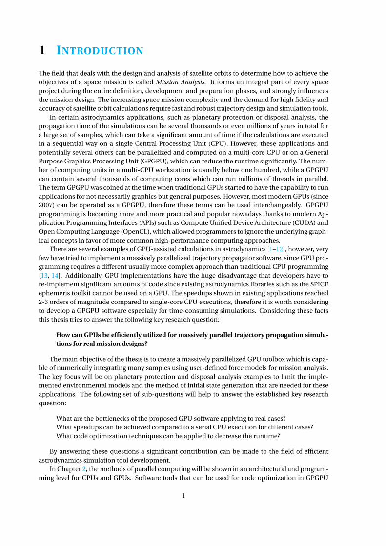
In the distributed memory model, large-scale computational engines or clusters are constructedfrom many processors or nodes connected by a network. Each processor which executes a set oftasks uses their own local memory, and processors can communicate the contents of their localmemory over the network by sending and receiving messages. Therefore, this model is often calledMessage Passing Model as well. Figure 2.5 shows a typical cluster with distributed memory.
Processor
Cache Cache
Memory Memory
Interconnection Network
Memory
Cache
Processor Processor......
......
......
Figure 2.5: The Distributed Memory Model [15].
From a programming perspective, distributed memory or message passing implementationsusually comprise a library of subroutines, and the calls to these subroutines are embedded in thesource code, thus the programmer is responsible for determining all parallelism. Message PassingInterface (MPI) is one of the most widely used APIs that is available for this method.
HYBRID MEMORY MODEL
The hybrid memory model combines the previously described models. A common usage of thismodel is the combination of MPI with OpenMP, where the threads on each node are handled byOpenMP and the communication between processes on different nodes occurs over the networkusing MPI. Another popular example of the hybrid model is using the combination of MPI withCUDA in multi CPU–GPU environments.

2.3. COMPUTER MEMORY TYPES 7
2.3. COMPUTER MEMORY TYPESThere are many different types of computer memory which are used nowadays, but the ones thatusually store data and machine code are the so-called Random Access Memory (RAM). This type ofmemory has been available since the 1970s and allows data items to be read or written in almostthe same amount of time irrespective of the physical location of data inside the memory. The twowidely used forms of RAM are the Static Random Access Memory (SRAM) and the Dynamic RandomAccess Memory (DRAM), which can be found in almost every CPU and GPU.
2.3.1. STATIC RANDOM ACCESS MEMORY
This type of memory is usually used as a cache memory. It uses flip-flops as building blocks whichare made of transistors such as MOSFETs, therefore this type of memory is rather simple, reliable,very fast, and usually has a low power consumption. However, SRAM has a low storage capacity(8-30 MB) and it is much harder to manufacture than DRAM.
2.3.2. DYNAMIC RANDOM ACCESS MEMORY
This type of memory is usually used as the main memory of a computer. It does not use transistorsas building blocks to store the data, but small capacitors within an integrated circuit. Because of thistype of storage the data has to be refreshed (read and put back), since these small capacitors leakafter a certain amount of time. There are different type of execution time delays e.g. the refreshingdelay, precharge delay, row-to-row delay which are specified by the memory interface standardssuch as the ubiquitous Double Data Rate Fourth-Generation Synchronous Dynamic Random AccessMemory (DDR4 SDRAM). Due to these significant delays, the data is accessed in big rows at a time,(2-8 kB), although once the row is read, the access to that row is extremely fast via a row buffer.Because of this method, the latency to access subsequent elements in the same row is much fasterthan accessing elements which are scattered in the memory. This feature has serious implications ina way of programming data access patterns in an application. Compared to SRAM, DRAM is muchcheaper to produce, and it can have much larger capacity (16-64 GB).
2.4. METRICS FOR PERFORMANCE MEASUREMENTThere are many ways to measure the efficiency and performance of hardware and software. In par-allel computation and parallel programming the following metrics are most common:
Latency is the time it takes for an operation to start and complete, and is usually expressed in mi-croseconds. Generally every architecture aims to decrease latency, however it is commonlysaid that CPUs are latency-optimized hardware.
Bandwidth is the amount of data that can be processed per unit of time, and is usually expressedin MB/s (megabytes/sec) or GB/s (gigabytes/sec). It is an important metric of the memorycomponents (DRAM, SRAM) or the data transfer bus (Peripheral Component InterconnectExpress (PCIe)). Every architecture aims to increase its bandwidth.
Throughput is the number of operations that can be processed per unit of time, and is commonlyexpressed in billion floating-point operations per second (GFLOPS). In accordance to CPUswhich optimize for latency, GPUs optimize for throughput.
Threading Efficiency quantifies how additional software threads are improving program perfor-mance relatively, and can be calculated as follows [16]:
Threading Efficiency = Single-Thread Execution Time
(N-Thread Execution Time)×N(2.1)

8 2. PARALLEL COMPUTING MODELS
where N is the number of threads. It can be seen that if 100% threading efficiency is achieved,the execution time reduces by the number of the launched threads. However, due to limita-tions in the resources of the hardware, 100% threading efficiency cannot usually be achieved.
Parallelization Overhead quantifies the cost of parallelization and is defined as follows [16]:
Parallelization Overhead = 1−Threading Efficiency (2.2)
Speedup is the improvement in execution time of a task executed on two systems processing thesame problem. It is simply calculated as the ratio of the execution times in the two systems,however there are more sophisticated speedup definitions which take latency or throughputof the executions into account. It is desired to achieve speedups that are larger than one.
2.5. MULTI-CORE CPU ARCHITECTUREMost modern CPUs are designed in such a way that each of their cores is capable of executing morethan one thread at the same time. The consequence of this concurrent execution is that the threadshave to share some of the resources, such as the cache memory within the core. The cores canexecute two threads in most of the commercially available CPUs such as the Intel Core i7 family.The core and thread numbers of a CPU are usually denoted as e.g. 6C/12T, which stands for sixcores and twelve threads. In this report, under the term CPU, usually a multi-core multi-thread out-of-order processor is meant. Note that there are existing in-order many-core CPUs such as the IntelXeon Phi family, which have approximately 60 cores and 240 threads. The internal architecture of aconsumer modern CPU such as the Intel Core i7 family as well as the connection with a GPU andthe main memory can be seen in Figure 2.6.
CORE 1
L3$ 15 MB
QU
EUE,
UN
CO
RE,
I/O
DD
R4
MEM
OR
Y C
ON
TRO
LLER
DD
R4
MAI
N M
EMO
RY
64G
B
CORE 2 CORE 3
CORE 4 CORE 5 CORE 6
PCI EXPRESS BUS
MEMORY BUS
CPU
GPU GPU X99 chipset
Figure 2.6: The architecture of a 6C/12T CPU with external PCIe connection to multiple GPUs and memory bus to themain memory [16].

2.5. MULTI-CORE CPU ARCHITECTURE 9
As presented in the figure, in this particular CPU there are six cores which share the 15 MB L3cache. It will be shown later that the L3 cache is absent in a GPU, however it is a crucial part of aCPU since it takes up almost 20% of the CPU die area. The purpose of the cache memory is to storesome particular data so future requests for that data can be served faster. The data stored in a cachemight be the result of an earlier computation, or the duplicate of data stored elsewhere. Usually, theprogrammer has no input in the way the cache memory manages its data, however by smart datademand patterns there is some control of the efficiency of the cache.
As shown in Figure 2.6, there is no direct access path from the cores to the main memory, whichin this example has a type of DDR4 and a size of 64 GB. The memory controller takes up a signif-icant chip area and buffers and aggregates the data coming from the L3 cache trying to excludethe inefficiencies of the block-transfer nature of the DRAM. It is also responsible for converting thedata streams between the L3 cache and the DRAM into a proper format. This is necessary since theDRAM works with rows of data, and the L3 cache, which is an SRAM, works with one line at a time.The size of the cache line is different for each processor. A typical value is 64 bytes for modern CPUs.
The queue, uncore, I/O box seen at the left side of the figure is responsible for communicationwith the chipset (X99 in this particular example) which uses PCIe to communicate with the GPUs.It is also responsible for queuing and efficiently transferring the data between the L3 cache and thePCIe bus.
To summarize, three main parts of the CPU can be distinguished: the cores, the memory, andthe I/O, thus the programs that a CPU executes can be core-intensive, memory-intensive and/orI/O-intensive. A core-intensive program heavily uses the core’s resources, which means it is able toperform a large number of arithmetic or floating-point calculations. A memory-intensive programuses the memory controller heavily and has a large amount of data transfer between the CPU andthe main memory. An I/O-intensive program uses the I/O controller of the CPU and communicateswith the peripheral components of the computer such as the GPU.
CPU CORE
The general structure of a modern out-of-order CPU core with some typical sizes of the cache mem-ory can be seen in Figure 2.7.
L1 I$ 32KB
L2$ 256KB
L1 D$ 32KB
L3$ 15MB
Execution Units
Thread 2 Hardware
Thread 1 Hardware
Pre-fetch
Decode
ALU
ALU FP ADD
ALU FP MUL MUL/DIV
LAGU SAGU MOB
Figure 2.7: The architecture and execution units of a core within a 6C/12T CPU [16].

10 2. PARALLEL COMPUTING MODELS
It can be seen that two of the three levels of cache (L1, L2) are private within each core, howeveras shown before, the L3 cache is shared between all cores. Generally, there is an improvement inbandwidth and latency of a factor of 10-20 when moving to a lower-level cache. However, as notedin Figure 2.7, the size of the cache decreases with increasing cache level. In this particular example,each core has 64 kB L1 and 256 kB L2 cache memory, and the CPU has a 15 MB L3 cache sharedbetween the cores.
The L1 cache is broken up into two separate segments: the 32 kB instruction cache (L1I) whichstores the most recently used CPU instructions, and the 32 kB data cache (L1D) which stores a copyof certain data elements.
The L2 and L3 cache can be used either for instructions or for data. Usually the data goesthrough each of the cache levels that is supervised by cache memory controller logic, which can-not be controlled by the programmer, in contrast with CUDA programming, where the programmerhas a little freedom of changing which data segment can be moved into cache.
It can be seen in Figure 2.7 that this core is capable of executing two threads, however eachthread shares most of the resources such as the cache or the execution units within the core. Theirdedicated hardware, which is denoted as Thread 1 Hardware and Thread 2 Hardware, primarilyconsists of register files.
The execution units are responsible for every calculation that is done inside a CPU core as wellas the memory address generation to write the data from both threads back into the memory. Theacronyms of the execution units are the following:
• ALU (Arithmetic Logic Unit)• FPU (Floating Point Unit)• FPMUL (Floating Point Multiplier)• FPADD (Floating Point Adder)• MUL/DIV (Dedicated Multiplier/Divider)• LAGU (Load Address Generation Unit)• SAGU (Store Address Generation Unit)• MOB (Memory Order Buffer)
The ALUs are responsible for integer and logic operations, and the FPUs are responsible forfloating-point operations. However, because floating-point addition, multiplication and divisionare much more complex than their integer versions, they have their dedicated hardware compo-nents within the core (FPMUL, FPADD, MUL/DIV). Memory addresses that the threads generateare calculated within LAGU and SAGU, and they are properly ordered in the MOB.
The prefetcher and decoder components are responsible to decode and route the instructionstowards the thread that should execute that particular instruction, therefore they are also shared byboth threads [16].
2.6. GPU PARALLELISM
2.6.1. HISTORY OF GPUS AND GPGPUS
Around the 1980s and 1990s it became evident that there was a need for a new type of processorwhich is especially suitable for 2D and 3D graphics applications which requires a large numberof floating-point operations. Graphically-driven operating systems such as Microsoft Windows be-came extremely popular and there was a growing need for better visualization in the computer gam-ing industry. Silicon Graphics, NVIDIA, ATI Technologies and other companies started to producegraphics accelerators that were affordable enough to attract widespread attention and gave birth tothe term GPU [17].
The early GPU designs were created specifically for 2D and 3D graphics calculations but theconcept of using them for general purposes was not yet considered. 3D applications used trianglesto associate a texture for a surface of any object instead of using pixels as a 2D application would

2.6. GPU PARALLELISM 11
do, therefore dedicated hardware components were optimized to calculate these image coordinateconversions, 3D to 2D conversions and mappings much faster. The main steps to move a 3D objectin an application can be seen in Figure 2.8.
Figure 2.8: Steps to move triangulated 3D objects [16].
There are four key parts of moving a 3D object. First, the GPU has to deal with triangles as a nat-ural data type for a 3D object, and has to create a so-called wire frame which contains the locationand the texture of each triangle (Box I). However, before an object’s new position is calculated thelocation and the texture of its triangle representation is decoupled, because for the position calcu-lations the texture does not have to be taken into account. The texture of each triangle is stored ina dedicated memory area called texture memory. As a second step, heavy floating-point operationsare performed on each triangle to move the wire frame (Box II). As a third step, before displayingthe moved object, a texture mapping step fills the triangles with their associated texture, turningthe wire-frame back into an object (Box III). As a last step, a 3D-to-2D transformation has to be per-formed to display the object as an image on the computer screen, because every computer screenis composed of 2D pixels [16].
The native API for graphics cards was Open Graphics Library (OpenGL), which was created bySilicon Graphics in 1992, or DirectX, which was created by Microsoft in 1995. These GPU languagesincorporated all the aforementioned steps and therefore were not suited for general-purpose GPUprogramming since a programmer had to trick the GPU that each calculation is performed on a 3Dobject and completely unnecessary calculations had to be performed such as texture mapping and3D to 2D mapping. Furthermore, the early GPUs did not support double-precision computationswhich is necessary for scientific computations or other applications that require higher accuracy.
In the late 1990s, GPU manufacturers were small companies that saw GPUs as ordinary add-oncards that were no different than hard-disk controllers, sound cards, or modems. However, somecompanies realized that there has been a growing interest in general-purpose computations usingGPUs and they started developing hardware and APIs that can serve these new applications.
For efficient GPGPU programming, bypassing the graphics functionality (indicated with Boxes I,III, and IV in Figure 2.8) was necessary, while Box II remained the only fundamental block for scien-tific computations. However, Boxes I, III and IV were not eliminated and could be accessed still forgraphics applications. It was also necessary to allow the GPGPU programmers to input data directlyinto Box II without having to go through Box I. Furthermore, a triangle was not a comfortable datatype for scientific computations, suggesting that the natural data types in Box II had to be the usualintegers, float, and double [16].
By the mid 2000s new APIs had emerged which allowed to create program code on a GPU forgeneral purposes. The two predominant desktop GPU languages are CUDA, which is designed only

12 2. PARALLEL COMPUTING MODELS
for NVIDIA platforms, and OpenCL, which can be used in different GPUs, and also works on Field-Programmable Gate Arrays (FPGAs) and Digital Signal Processors (DSPs). In Section 2.6.3, onlyCUDA will be described in more detail since it will be used in this thesis project because it is moredeveloper friendly, it has its own debugger (CUDA-GDB) and many other features despite it is onlycompatible with NVIDIA GPUs. Additionally, this report will focus on NVIDIA GPU architecturessince they are the most popular and powerful CUDA-capable GPGPUs nowadays.
2.6.2. GPU ARCHITECTURES
In contrast with a general CPU architecture, a general GPU architecture cannot be described sinceit has changed significantly on several occasions over the past one or two decades. NVIDIA hasdeveloped various different architectures since their first GPGPU was produced, however there aresome similarities in all of them as they are primarily designed as an SIMD architecture. The NVIDIAarchitectures in chronological order are the following [16]:
• Tesla• Fermi• Kepler• Maxwell• Pascal• Volta• Turing
As mentioned before, the GPUs are designed for massively parallel computing, thus the hard-ware itself can host up to several thousands of cores inside them. However, these cores are muchsimpler than a CPU core and take up much smaller chip area. The clock speed of a GPU core is alsomuch lower, a typical value is 1-1.5 GHz, while a modern CPU core’s clock speed can reach 4 GHz.
To allow the execution of a huge number of threads, GPU designers had to invent new additionalhierarchical organizations of threads, which are the following:
Warp is a group of 32 threads, which execute the same instructions concurrently. It infers that inany GPU program it is recommended to launch at least 32 or any multiple of 32 number ofthreads, because executing 1 or 32 threads takes exactly the same amount of time.
Block is a group of 1 to 32 warps. This means that the maximum number of threads within oneblock is 1024. A block should be designed as an isolated set of threads that can execute inde-pendently from other blocks to achieve the highest efficiency in parallel computing.
Grid is simply a group of blocks. The maximum number of blocks within a grid is different for eachGPU architecture.
To execute these new organizations of threads at their hardware representations, new structureswere created at an architectural level as well. Each thread is executed by a core or sometimes calledCUDA core, and each block is executed by a Streaming Multiprocessor (SM). Note that in the Keplerarchitecture the SM was re-named to Next Generation Streaming Multiprocessor (SMX), and in theMaxwell architecture it was re-named again to Maxwell Streaming Multiprocessor (SMM), howeverfor the Pascal, Volta, and Turing families it is called SM again. Each SM is grouped in a TextureProcessing Cluster (TPC), which for some earlier (e.g. Fermi) generations is the same as the SM.TPCs (or SMs) are grouped in a Graphics Processing Cluster (GPC).
The number of cores and SMs as well as the size of the caches changed with every new genera-tion, and even within generations. In each generation NVIDIA named their chips with a codename(e.g. GP100, GP102, etc. which are variations of a Pascal architecture) as well as a family name(e.g. Tesla P100) for the actual model. The highest values of the cores and cache sizes, and eacharchitectural family’s introduction year are tabulated in Table 2.1.

2.6. GPU PARALLELISM 13
Table 2.1: NVIDIA microarchitecture families and their hardware features [16].
Family (chip) Intro year Cores/SM Total SMs Total cores L1$ (kB) L2$ (kB)Tesla (GT200) 2006 8 30 SMs 240 241 256Fermi (GF110) 2009 32 16 SMs 512 481 768Kepler (GK110) 2012 192 15 SMXs 2880 481 1536
Maxwell (GM200) 2014 128 24 SMMs 3072 24 3072Pascal (GP100) 2016 64 60 SMs 3840 24 4096Volta (GV100) 2017 64 84 SMs 5376 1281 6144
Turing (TU102) 2018 64 72 SMs 4608 961 61441 Same on-chip memory is used for both L1$ and shared memory, the L1$ size can be configured.
In the following parts of this section, the internal structure of the Fermi and Pascal architecturesand their SMs will be discussed. The Fermi architecture can be considered as an obsolete architec-ture today, however it is simple enough to represent and explain the general features of a GPU. Thedescription of the Pascal architecture will show the improvements that NVIDIA made to optimizetheir hardware for scientific computations. It is also important to mention that over the course ofthe thesis project high-end Pascal architecture GPUs, such as the Tesla P100, have been used fortesting purposes.
FERMI ARCHITECTURE
The internal structure of a typical Fermi SM (GF110) and CUDA core can be seen in Figure 2.9.
Core Core
Core Core
Core Core
Core Core
Core Core
Core Core
Core Core
Core Core
Core Core
Core Core
Core Core
Core Core
Core Core
Core Core
Core Core
Core Core
LD/ST LD/ST
LD/ST LD/ST
LD/ST LD/ST
LD/ST LD/ST
LD/ST LD/ST
LD/ST LD/ST
LD/ST LD/ST
LD/ST LD/ST
SFU
SFU
SFU
SFU
128KB Register File (32768 x 32-bit Registers)
64KB Cache : Shared Memory + L1$
Instruction Cache
Warp Scheduler
Dispatcher
Warp Scheduler
Dispatcher
Core
FP INT
Dispatch
Operands
Result Q
Figure 2.9: The internal architecture of a Fermi Streaming Multiprocessor (GF110) [16].
This SM contains 32 cores or CUDA cores which are only responsible for integer and floating-point operations and are fairly simpler than the CPU cores. The INT and FP units inside the core areequivalent to an ALU and FPU inside a CPU core. Each FP unit is capable of double-precision com-putations, however they are much slower than their CPU versions. Each GPU core has a dispatchport, which is responsible to receive the next instruction. The operand collector port receives itsoperands from the register file. The cores also have a result queue, to which they write their results,

14 2. PARALLEL COMPUTING MODELS
which will be committed to the register file eventually.There are two warp schedulers inside this SM which are responsible to turn the blocks into a set
of warps and schedule them to be executed by the execution units. The schedulers are playing animportant role in the so-called latency hiding effect which will be explained in more detail in Section2.6.6. The Dispatcher units dispatch a warp and pass their ID information to the cores, when theresources are available for that. Note the important concept that warps may execute serially becausethere is simply not enough cores to execute hundreds of thousands or even more threads in parallel.Although programmers should write their code with the assumption of each block and each warpexecuting independently, sometimes they are forced to use explicit synchronization for memoryreads that occur at intra-warp boundaries.
The execution units, similarly to the CPUs, are the CUDA cores themselves. The load/store units(LD/ST) are used to queue memory load/store requests, and Special Function Units (SFUs) are usedto calculate values for transcendental functions such as sin(), cos() or log(). When a memory read orwrite instruction needs to be executed, these memory requests are queued up in the LD/ST units,and when they receive the requested data, they make it available to the requesting instruction.
Instructions need to access a large number of registers, however in contrast to a CPU, all thecores inside an SM share a large register file, which in this case contains 32768 32-bit registers sum-ming up to 128 kB. The importance of register usage in CUDA programs will be discussed in Section2.6.8 in more detail.
The Instruction Cache holds the instructions within the block, while the L1 cache is responsiblefor caching commonly used data, which is also shared with another type of cache memory namedShared Memory, which will be discussed in Section 2.6.4. In this particular example the total firstlevel cache is 64 kB, which can be split between the L1 cache and the shared memory as either (16kB + 48 kB), (32 kB + 32 kB), or (48 kB + 16 kB). In contrast with the CPU cache the L1 cache memoryareas are not coherent which means that the L1 memory areas in each SM are disconnected fromeach other and the memory addresses do not necessarily refer to exactly the same memory areas.This difference makes the L1 cache even faster than the CPU cache. The cache line of the L1 cacheis 128 bytes [18].
The general internal architecture of a simple Fermi GPU (GF116) can be seen in Figure 2.10,which in this case contains 6 SMs. Note that a high-end Fermi GPU (GF110) can host up to a maxi-mum of 16 SMs.
L1$L1$L1$
L1$L1$ L1$
SM
0
L2$ 768KB
HO
ST
INTE
RFA
CE
GD
DR
5M
EM
OR
Y C
ON
TRO
LLER
GLO
BAL
MEM
OR
Y 1
GB
PCI EXPRESS BUS
MEMORY
BUS
GPU
X99 chipset CPU
SM
1
SM
2
SM
3
SM
4
SM
5
GIG
A TH
REA
DS
CH
EDU
LER
Figure 2.10: The internal architecture of a Fermi GPU (GF116) with external PCIe connection to the CPU and memory busto the main memory [16].
2.6. GPU PARALLELISM 15
Since it is possible to launch more threads on a GPU than its core numbers, a scheduler isneeded. This scheduling process is done by the Giga Thread Scheduler (GTS), which is responsiblefor assigning each block, based on which SM is available at the time of the assignment. For differentarchitectures there is a limit of how many blocks and how many threads can be executed in an SM,which is a very important metrics for optimization purposes, since the programmer can decide howmany threads could be in one block. This optimization method will be discussed in Section 2.6.8.
The memory controller communicates with the main memory, which is called global memoryin GPU programming. It it of a similar type as the CPU main memory (DRAM), however it is opti-mized for parallel computations, hence the GDDR5 name, where ’G’ stands for graphics. One bigdifference with the CPU architecture is that there is no L3 cache in a GPU, which makes the L2 cachethe Last Level Cache (LLC). The L2 cache in a GPU is coherent, similarly to a CPU L2 cache, howeveras an LLC it is much smaller than the LLC in a CPU, which was the L3 cache. The typical size of theLLC in a GPU is 1-6 MB (768 kB in this case), while it can reach 15 MB in a modern CPU.
The host interface is responsible for interfacing the PCIe bus via the X99 chipset, which is verysimilar to the I/O controller of a CPU. It allows to transfer data between the GPU and the CPU, whichis crucial for heterogeneous programming that will be explained in Section 2.6.3.
PASCAL ARCHITECTURE
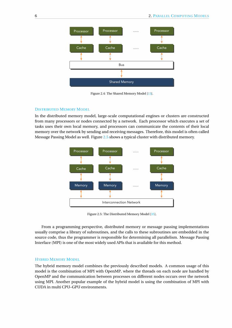
The Pascal architecture is not the most recent architecture family since Volta and Turing came out in2017 and 2018, however as mentioned before, high-end computing accelerators (Tesla P100, QuadroGP100) have been used in the thesis project, thus this architecture can be considered as representa-tive and will be described in more detail. An example of the internal structure of a Pascal scientificaccelerator card’s SM (GP100) can be seen in Figure 2.11.
SFUSFU
SFU
SFUSFU
SFU
SFUSFU
LDSTLDST
LDSTLDST
LDST
LDSTLDST
LDST
Warp Scheduler
Dispatcher
128KB RF (32768 x 32-b)
Instruction Buffer
CoreCore
CoreCore
Core
Core
CoreCore
CoreCore
Core
CoreCore
CoreCore
Core
DPUDPU
DPUDPU
DPUDPU
DPUDPU
CoreCore
CoreCore
Core
Core
CoreCore
CoreCore
Core
CoreCore
CoreCore
Core
DPUDPU
DPUDPU
DPUDPU
DPUDPU
Dispatcher
Instruction Cache
64KB Shared Memory
Texture / L1$
SFUSFU
SFU
SFUSFU
SFU
SFUSFU
LDSTLDST
LDSTLDST
LDST
LDSTLDST
LDST
Warp Scheduler
Dispatcher
128KB RF (32768 x 32-b)
Instruction Buffer
CoreCore
CoreCore
Core
Core
CoreCore
CoreCore
Core
CoreCore
CoreCore
Core
DPUDPU
DPUDPU
DPUDPU
DPUDPU
CoreCore
CoreCore
Core
Core
CoreCore
CoreCore
Core
CoreCore
CoreCore
Core
DPUDPU
DPUDPU
DPUDPU
DPUDPU
Dispatcher
Figure 2.11: The internal architecture of a Pascal Streaming Multiprocessor (GP100) [16].
It can be seen that this SM is partitioned into two processing blocks, each having 32 CUDA cores.There is a Double Precision Unit (DPU) for every two cores, which support conventional Instituteof Electrical and Electronics Engineers (IEEE) double-precision arithmetic. This means that just asa modern CPU, the execution time of a double-precision calculation is twice the time of a single-precision calculation. For previous GPU generations and gaming GPUs this ratio is much higher.However, as depicted in the figure, the DPU itself takes more chip area than one CUDA core. This
16 2. PARALLEL COMPUTING MODELS
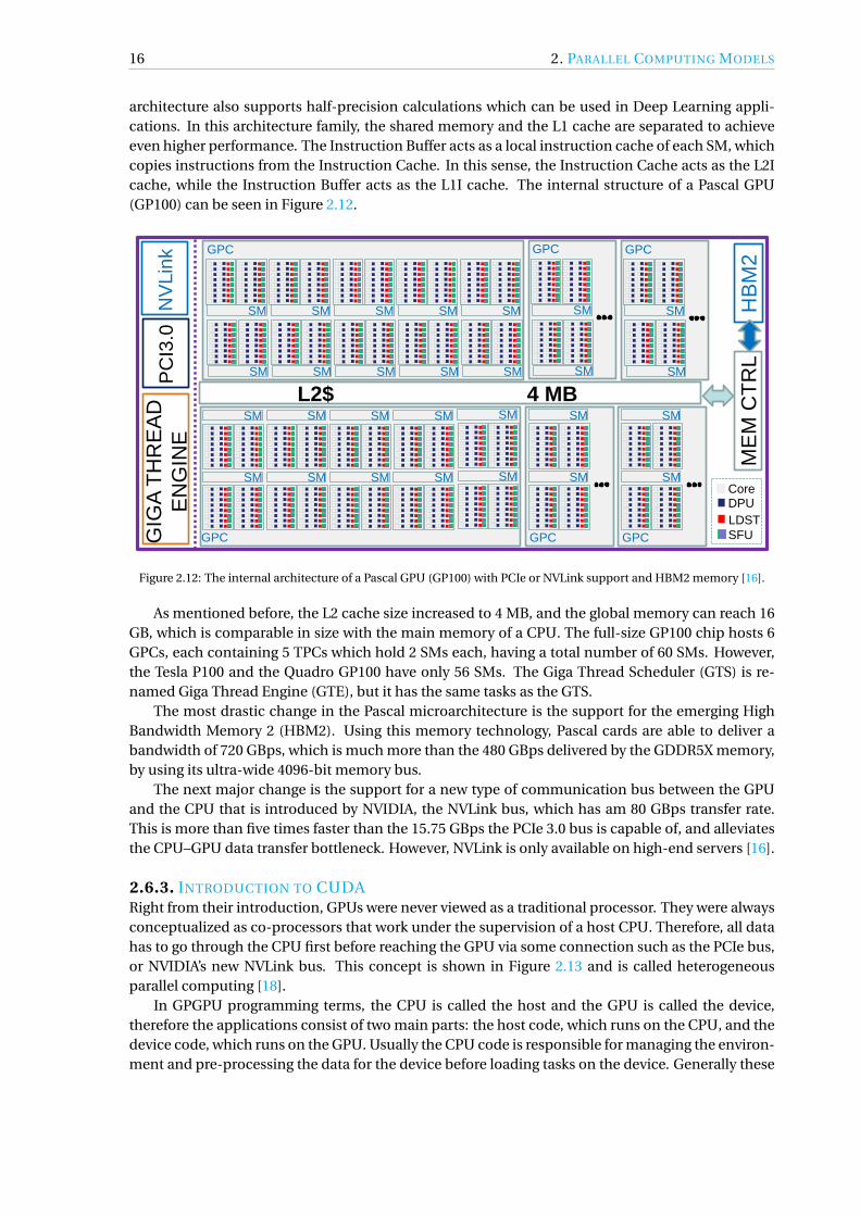
architecture also supports half-precision calculations which can be used in Deep Learning appli-cations. In this architecture family, the shared memory and the L1 cache are separated to achieveeven higher performance. The Instruction Buffer acts as a local instruction cache of each SM, whichcopies instructions from the Instruction Cache. In this sense, the Instruction Cache acts as the L2Icache, while the Instruction Buffer acts as the L1I cache. The internal structure of a Pascal GPU(GP100) can be seen in Figure 2.12.
L2$ 4 MB
PC
I3.0
ME
M C
TR
L
GIG
A T
HR
EA
D
EN
GIN
E
Core
LDST
DPU
SFU
SM
SM
SM
SM
SM
SM
SM
SM
SM
SM
GPC
SM
SM
GPC
SM
SM
GPC
GPC
SM
SM
SM
SM
SM
SM
SM
SM
SM
SM
SM
SM
GPC
SM
SM
GPC
NV
Lin
k
HB
M2
Figure 2.12: The internal architecture of a Pascal GPU (GP100) with PCIe or NVLink support and HBM2 memory [16].
As mentioned before, the L2 cache size increased to 4 MB, and the global memory can reach 16GB, which is comparable in size with the main memory of a CPU. The full-size GP100 chip hosts 6GPCs, each containing 5 TPCs which hold 2 SMs each, having a total number of 60 SMs. However,the Tesla P100 and the Quadro GP100 have only 56 SMs. The Giga Thread Scheduler (GTS) is re-named Giga Thread Engine (GTE), but it has the same tasks as the GTS.
The most drastic change in the Pascal microarchitecture is the support for the emerging HighBandwidth Memory 2 (HBM2). Using this memory technology, Pascal cards are able to deliver abandwidth of 720 GBps, which is much more than the 480 GBps delivered by the GDDR5X memory,by using its ultra-wide 4096-bit memory bus.
The next major change is the support for a new type of communication bus between the GPUand the CPU that is introduced by NVIDIA, the NVLink bus, which has am 80 GBps transfer rate.This is more than five times faster than the 15.75 GBps the PCIe 3.0 bus is capable of, and alleviatesthe CPU–GPU data transfer bottleneck. However, NVLink is only available on high-end servers [16].
2.6.3. INTRODUCTION TO CUDARight from their introduction, GPUs were never viewed as a traditional processor. They were alwaysconceptualized as co-processors that work under the supervision of a host CPU. Therefore, all datahas to go through the CPU first before reaching the GPU via some connection such as the PCIe bus,or NVIDIA’s new NVLink bus. This concept is shown in Figure 2.13 and is called heterogeneousparallel computing [18].
In GPGPU programming terms, the CPU is called the host and the GPU is called the device,therefore the applications consist of two main parts: the host code, which runs on the CPU, and thedevice code, which runs on the GPU. Usually the CPU code is responsible for managing the environ-ment and pre-processing the data for the device before loading tasks on the device. Generally these

2.6. GPU PARALLELISM 17
Control
Cache
DRAM DRAM
CPU GPU
PCle Bus
ALU
ALU ALU
ALU
Figure 2.13: Heterogeneous architecture [15].
program sections exhibit a rich amount of data parallelism, therefore GPUs are often considered ascomputing accelerators.
In November 2006, NVIDIA introduced CUDA, a general-purpose parallel computing platformand programming model that leverages the parallel computing engine in NVIDIA GPUs to solvemany complex computational problems in a more efficient way than on a CPU. The biggest advan-tage of CUDA is that it comes with a software environment that allows developers to use C/C++ asa high-level programming language; however other languages such as Fortran or Python are alsosupported by third-party developers.
NVIDIA developed its own CUDA compiler called nvcc, which separates the device code fromthe host code during the compilation process. As shown in Figure 2.14, the CPU host code is stan-dard C/C++ code and is further compiled with C compilers such as gcc. The device code is writtenusing the language extensions that are provided in CUDA. The data-parallel functions are calledkernels, and they are always executed on the device. The device code is further compiled by nvcc.During the link stage, CUDA runtime libraries are added for kernel procedure calls and explicit GPUdevice manipulation [15].
CUDA Libraries
CUDA Compiler
CPU Host Code
C Compiler
CPU
CUDA Assemblyfor Computing (PTX)
CUDA Driver& Runtime
DebuggerProfiler
GPU
Integrated CPU+GPU Code
Figure 2.14: CUDA nvcc compilation structure [15].
CUDA PROGRAM STRUCTURE
The execution of a typical simple CUDA program consists of five main parts:
1. Allocate GPU memory
2. Copy data from CPU memory to GPU memory

18 2. PARALLEL COMPUTING MODELS
3. Launch CUDA kernel from the CPU to perform program-specific computations
4. Copy data back from GPU memory to CPU memory
5. Free GPU memory
This structure shows the biggest advantage of CUDA, which is that the parallelism is inherent inthe kernel call, thus programmers can write their code in a traditional "serial" way. Note that notevery program requires all five steps for execution.
Generally, program designers should avoid many CPU–GPU memory copies in their applica-tions, because the bandwidth of the PCIe or even the NVLink bus is significantly smaller than thebandwidth of the GPU or CPU memory as shown in Figure 2.15.
CPU
GPUGDDR5X480 GB/s
PCIe16 GB/s
GPU Memory
CPU Memory
NVLink80 GB/s
HBM2720 GB/s
Figure 2.15: CPU–GPU memory connectivity [15].
COMPUTE CAPABILITY
It was shown in the previous sections that NVIDIA has changed the internal architecture of its GPUswith every new generation. This architectural change at hardware level requires significant changesin the API, therefore NVIDIA introduced the term Compute Capability. For every CUDA-capableGPU, it is specified which Compute Capability number they support. Compute Capability is back-ward compatible, therefore newer cards can execute code written for previous generations.
NVIDIA tries to make two improvements in every new architectural generation and ComputeCapability. First, the introduction of a new set of instructions that perform operations that couldnot have been performed in the previous Compute Capability, and second, performance improve-ments for all instructions that were introduced in the previous Compute Capability generations.This means that a program which was compiled with an older Compute Capability and runs on anewer architecture will likely perform better than on the same architecture.
Some important features such as dynamic parallelism, unified memory, half-precision floating-point number support were introduced in later Compute Capabilities, which were not available inolder generations. A detailed summary of the differences between the Compute Capabilities canbe found in [18]. The Compute Capability version of a particular GPU should not be confused withthe CUDA version (e.g., CUDA 7.5, CUDA 8, CUDA 9), which is the version of the CUDA softwareplatform [18].
THREAD HIERARCHY
CUDA provides a thread hierarchy abstraction to enable the organization of threads. This is a two-level thread hierarchy decomposed into blocks of threads and grids of blocks, as mentioned in Sec-tion 2.6.2. Note that warps are not part of this abstraction. The structure of this thread hierarchycan be seen in Figure 2.16.

2.6. GPU PARALLELISM 19
Block (1, 1)
Thread(0, 0)
Thread(1, 0)
Thread(2, 0)
Thread(3, 0)
Thread(4, 0)
Thread(0, 1)
Thread(1, 1)
Thread(2, 1)
Thread(3, 1)
Thread(4, 1)
Thread(0, 2)
Thread(1, 2)
Thread(2, 2)
Thread(3, 2)
Thread(4, 2)
Kernel
Grid
Block(0, 0)
Block(1, 0)
Block(2, 0)
DeviceHost
Block(0, 1)
Block(1, 1)
Block(2, 1)
Figure 2.16: Thread hierarchy in CUDA [15].
It can be seen in the figure that threads can be organized in more than one dimension, and eachblock and each thread has its unique ID. A grid is executed by a kernel on the GPU and all threadsin a grid share the same global memory space, named global memory. A block is executed on anSM, therefore the threads within one block can use the shared memory and can use block-localsynchronization. Threads within different blocks cannot cooperate. The threads are executed onthe CUDA cores, as visualized in Figure 2.17.
Software
Thread
Thread Block
Grid
Hardware
CUDA Core
SM
Device
Figure 2.17: Software and hardware abstraction in CUDA [15].

20 2. PARALLEL COMPUTING MODELS
In order to launch a kernel, the programmer has to specify the number of blocks per grid andthe number of threads per block. It is also the programmer’s task to specify the dimensionality ofthe thread hierarchy. An important feature of CUDA kernel launches is that they are asynchronous,which means that the control returns to the CPU immediately after the CUDA kernel is invoked.However, the programmer can synchronize the GPU and the CPU, such that the CPU idles until thekernel is finished.
CUDA STREAMS
A CUDA stream refers to a sequence of asynchronous CUDA operations that execute on a GPU inthe order issued by the host code. Each stream executes every task in it serially as it was queued up.However, if there is any part between two streams that can be overlapped, the CUDA runtime en-gine automatically overlaps these operations. Therefore, although each stream is serially executedwithin itself, multiple streams can overlap execution in parallel. By using multiple streams to launchmultiple simultaneous kernels, grid-level concurrency can be implemented.
One of the common use cases of streams is to improve the performance of the host-to-deviceand device-to-host data transfer. As mentioned before, all kernel launches are asynchronous, thusit is possible that the host transfers some data to the device while a kernel is running on it. Figure2.18 illustrates a simple timeline of CUDA operations using three streams. Both data transfer andkernel computation are evenly distributed among three concurrent streams. It can be seen in thefigure, that the performance improvement can be rather significant using CUDA streams.
KernelMemory Copy (H2D)
H2D
Serial
ConcurrentPerformance improvement
time
time
H2D
H2D
K1
K2
K3
Memory Copy (D2H)
D2H
D2H
D2H
Figure 2.18: Composition of possible CUDA streams (H2D: Host to Device, D2H: Device to Host) [15].
The other usages of CUDA streams to reduce the runtime could be to overlap multiple, con-current kernels on the device or to overlap CPU execution and GPU execution. The application ofmany streams should be generally avoided because the synchronization between streams can berather complex, and the overutilization of hardware resources may result in kernel serialization.
2.6.4. CUDA MEMORY MODEL
There are many different types of memory in CUDA with different scopes, lifetime, and cachingbehaviour. These memory spaces are illustrated in Figure 2.19.
Each thread in a kernel has private local memory and can access the registers in a CUDA core.Each block has shared memory visible to all threads of the block, the contents of which persists forthe lifetime of the block. All threads have access to the same global memory. Additionally, there aretwo read-only memory spaces accessible by all threads: the constant memory, and the texture orsurface memory.
REGISTERS
Registers are the fastest memory space on a GPU and can be found inside the CUDA cores. Thedeclared variables and arrays in a kernel are generally stored in a register, and they are private to

2.6. GPU PARALLELISM 21
(Device) Grid
Block (0, 0)
Shared Memory
Registers
Thread (0, 0)
LocalMemory
LocalMemory
LocalMemory
GlobalMemory
ConstantMemory
TextureMemory
Host
Thread (1, 0) Thread (2, 0)
Registers Registers
Figure 2.19: Memory hierarchy in CUDA [15].
each thread. These register variables share their lifetime with the kernel, therefore they cannot beaccessed again after the kernel completes execution.
There is a hardware limit on the number of registers per thread for each GPU architecture, whichis a very important metric for optimization purposes. Using fewer registers in a kernel may allowmore blocks to reside on an SM, which increases occupancy and improves performance (see Section2.6.8). If a kernel has to use more registers than the hardware limit, then the excess registers will spillover to local memory, which will decrease performance. The maximum number of registers used bykernels can also be specified by the programmer in compilation time.
LOCAL MEMORY
Variables and arrays in a kernel that cannot fit into the register space allocated for that kernel will beplaced into local memory. Note that the values spilled to local memory reside in the same physicallocation as the global memory (e.g. GDDR memory), therefore local memory accesses have highlatency and low bandwidth. Programmers have to consider efficient memory access patterns to uselocal memory variables effectively.
SHARED MEMORY
Shared memory is accessible by each thread within a block and it has a much higher bandwidth andmuch lower latency than local or global memory. It is used similarly to the CPU L1 cache, but it isalso programmable, therefore it is often called software cache. Shared memory is declared in thescope of a kernel function but shares its lifetime with a block. When a block has finished executing,its allocation of shared memory will be released and assigned to other blocks.

22 2. PARALLEL COMPUTING MODELS
As mentioned in Section 2.6.2, in older architectures (Tesla, Fermi, Kepler) shared memory andthe L1 cache resided in the same physical memory, but this technique was changed in newer gen-erations (Maxwell, Pascal), however in the newest generations (Volta, Turing) the L1 cache and theshared memory reside in the same physical memory again. Regardless of the physical size of theshared memory, the maximum amount of it per block is limited by CUDA to 48 kB. In the Volta fam-ily, this limit has increased to 96 kB, however it is partitioned to 48 + 48 kB between statically anddynamically allocated memory. In the newest Turing family this value is 64 kB. As a programmer itis important to be careful to not over-utilize shared memory because that inadvertently limits thenumber of active warps, which causes lower occupancy and usually decreases performance.
Threads within a block can cooperate by sharing data stored in shared memory. However, accessto shared memory must be synchronized to avoid conflicts between the threads, which can be doneby the programmer.
CONSTANT MEMORY
Constant memory is a dedicated area in device memory, which is accessible for each thread andhas the best performance if the data stored in it is read multiple times by all threads in a warp. Thismemory region is designed to provide the same constant value to multiple threads. The program-mer can declare a variable which will be placed in constant memory, however it has to be declaredwith a global scope, outside of any kernels, to be visible to all kernels in the same compilation unit.Kernels can only read from the constant memory, therefore they must be initialized by the host.
The size of the constant memory is 64 kB for all Compute Capabilities, which can be cached ina dedicated per-SM constant cache. The amount of constant cache has varied slightly for differentGPU families (4-8 kB) [18]. The usage of constant memory in the implemented software will bedescribed in Chapter 7.
TEXTURE AND SURFACE MEMORY
Texture and surface memory (usually noted only as texture memory) is used mainly for graphicsapplications and has a rare usage in GPGPU programming. Texture memory is used for textureobjects and surface memory is used for surface objects. Texture memory resides in device memoryand is cached in a per-SM cache. In some generations, texture cache is separate from the L1 cache,but in newer generations they share the same cache area. Texture memory is optimized for 2Dspatial locality, so threads in a warp that use texture memory to access 2D data will achieve the bestperformance [15]. It will be shown in Section 7.5 that storing the ephemeris data in texture memoryleads to significant performance increment.
GLOBAL MEMORY
Global memory is the largest, highest-latency, and most commonly used memory on a GPU, whichcan be accessed on the device from any SM throughout the lifetime of the application. As mentionedbefore, global memory usually is a GDDR Random Access Memory (e.g. GDDR5), therefore it is bestto read consecutive larger chunks of data from global memory to achieve the highest efficiency.
A variable in global memory can either be declared statically or dynamically. Global memorycan be dynamically allocated and freed by the host using built-in CUDA functions. Pointers to globalmemory are then passed to kernel functions as parameters. Global memory allocations exist for thelifetime of an application and are accessible to all threads of all kernels. The programmers haveto be very careful when accessing global memory from multiple threads, since the thread execu-tion cannot be synchronized across blocks, and there is a risk of several threads in different blocksconcurrently modifying the same location in global memory, which will lead to undefined programbehaviour.

2.6. GPU PARALLELISM 23
PINNED MEMORY
Modern operating systems usually use virtual memory, which gives the illusion to the user that morethan the actual physical size of the memory is available. The operating system treats the requiredmemory as a set of pages, which are small chunks (e.g. 4 kB) of segments, and gives the applica-tions the virtual addresses. Memory allocation functions take care of the virtual-to-physical addresstranslations and all of this process is hidden from the user.
Every host memory allocation is pageable by default, which is subject to page fault operationsthat move data in host virtual memory to different physical locations as directed by the operatingsystem [15]. It is possible for a program to request physical memory directly, which is called pinnedor page-locked memory. The data transfer between the host and the device using pageable andpinned memory can be seen in Figure 2.20.
Pageable Data Transfer
Device
DRAM
PageableMemory
PinnedMemory
Host
Pinned Data Transfer
Device
DRAM
PinnedMemory
Host
Figure 2.20: Data transfer using pageable and pinned memory [15].
Allocating pinned memory has many benefits, however these allocations will start failing longbefore allocations in pageable memory. In addition, pinned memory allocations reduce the actualphysical memory available to the operating system for paging, which eventually decreases overallsystem performance.
There are different types of pinned memory for various applications, but all of them improvethe transfer speed between the host and the device, and usually the copies between the pinned hostmemory and the device memory can be performed concurrently with the kernel execution itself.
Portable pinned memory is useful in multi-device applications, since this type of memory isavailable on all devices, in contrast to the default pinned memory, which is only available on thedevice that was current when the memory was allocated.
Write-combining pinned memory frees up the L1 and L2 caches of the host, thus the transfer canbe faster via the PCIe bus. This type of memory is efficient for buffers that will be written by the hostand read by the device using either mapped pinned memory or host-to-device transfers [18].
Mapped pinned memory or zero-copy memory is a type of host memory that is mapped into thedevice address space, which eliminates the need to copy it to or from device memory. However,applications that have frequent read-write operations using zero-copy memory will be significantlyslower, since every memory transaction to mapped memory must pass over the PCIe bus, whichadds a large amount of latency. Additionally, mapped page-locked memory is shared between thehost and the device, thus the application must synchronize memory accesses to avoid any potentialhazards [15].
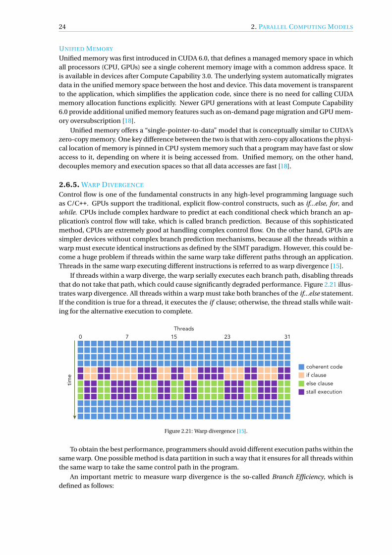
24 2. PARALLEL COMPUTING MODELS
UNIFIED MEMORY
Unified memory was first introduced in CUDA 6.0, that defines a managed memory space in whichall processors (CPU, GPUs) see a single coherent memory image with a common address space. Itis available in devices after Compute Capability 3.0. The underlying system automatically migratesdata in the unified memory space between the host and device. This data movement is transparentto the application, which simplifies the application code, since there is no need for calling CUDAmemory allocation functions explicitly. Newer GPU generations with at least Compute Capability6.0 provide additional unified memory features such as on-demand page migration and GPU mem-ory oversubscription [18].
Unified memory offers a “single-pointer-to-data” model that is conceptually similar to CUDA’szero-copy memory. One key difference between the two is that with zero-copy allocations the physi-cal location of memory is pinned in CPU system memory such that a program may have fast or slowaccess to it, depending on where it is being accessed from. Unified memory, on the other hand,decouples memory and execution spaces so that all data accesses are fast [18].
2.6.5. WARP DIVERGENCE
Control flow is one of the fundamental constructs in any high-level programming language suchas C/C++. GPUs support the traditional, explicit flow-control constructs, such as if...else, for, andwhile. CPUs include complex hardware to predict at each conditional check which branch an ap-plication’s control flow will take, which is called branch prediction. Because of this sophisticatedmethod, CPUs are extremely good at handling complex control flow. On the other hand, GPUs aresimpler devices without complex branch prediction mechanisms, because all the threads within awarp must execute identical instructions as defined by the SIMT paradigm. However, this could be-come a huge problem if threads within the same warp take different paths through an application.Threads in the same warp executing different instructions is referred to as warp divergence [15].
If threads within a warp diverge, the warp serially executes each branch path, disabling threadsthat do not take that path, which could cause significantly degraded performance. Figure 2.21 illus-trates warp divergence. All threads within a warp must take both branches of the if...else statement.If the condition is true for a thread, it executes the if clause; otherwise, the thread stalls while wait-ing for the alternative execution to complete.
coherent code
0 7 15Threads
23 31
if clause
else clausetim
e
stall execution
Figure 2.21: Warp divergence [15].
To obtain the best performance, programmers should avoid different execution paths within thesame warp. One possible method is data partition in such a way that it ensures for all threads withinthe same warp to take the same control path in the program.
An important metric to measure warp divergence is the so-called Branch Efficiency, which isdefined as follows:

2.6. GPU PARALLELISM 25
Branch Efficiency = #Branches−#Diverged Branches
#Branches(2.3)
Branch Efficiency is the ratio of uniform control flow decisions over all executed branch in-structions. The lower this metric, the more often warps split their control flow, which may leadto decreased overall execution performance. The nvprof profiling tool is capable of measuring theBranch Efficiency of an application [19].
If the number of instructions in the body of a conditional statement is less than a certain thresh-old, CUDA compiler optimization may be capable of replacing a branch instruction with predicatedinstructions, which would eliminate warp divergence. However, a longer code path will certainlyresult in warp divergence [15].
2.6.6. LATENCY HIDING
Latency hiding is an extremely important feature of GPGPU programming. Since every instructionhas a non-zero latency called instruction latency, which is defined as the number of clock cyclesbetween the instruction being issued and being completed, it is inevitable that a warp stalls dueto this latency. However, this latency can be hidden by utilizing parallelism. The warp schedulersinside an SM are capable of changing the control between warps, thus keep the SM busy with usefulwork at all times. In other words, GPU instruction latency can be hidden by computation by otherwarps. In Figure 2.22 Warp 0 stalls, and Warp Scheduler 0 picks up other warps (Warp 2 and Warp3) to execute and then executes Warp 0 when it is available again. On the bottom of the figure WarpScheduler 1 is unable to pick other warps when Warp 1 stalls.
Warp 3Warp 2
Warp 6 Warp 5
Time
Warp Scheduler 0
Warp Scheduler 1 Warp 1
no eligible warps toexecute
warp 0 waiting while SM still busy
Warp 0 Warp 0 Warp 4
Figure 2.22: Latency hiding [15].
When considering instruction latency only, two general basic instruction types can be distin-guished:
• Arithmetic instructions• Memory instructions
Arithmetic instruction latency is the time between an arithmetic operation start and the time whenits output is produced. Memory instruction latency is the time between a load or store operationissue and the data arrival at its destination. The corresponding latencies for each case are approxi-mately 5-20 cycles for arithmetic operations and 400-800 cycles for global memory accesses.
Using Little’s Law, the number of required active warps (threads) can be estimated to hide la-tency. Little’s law is the following [15]:
Number of Required Warps = Latency×Throughput (2.4)
Little’s Law is visualized in Figure 2.23. Suppose the average latency for an instruction in a kernel is5 cycles. To keep a throughput of 6 warps executed per cycle, at least 30 active warps are needed.It is desired to design the software such that it maximizes latency hiding to achieve the best perfor-mance.
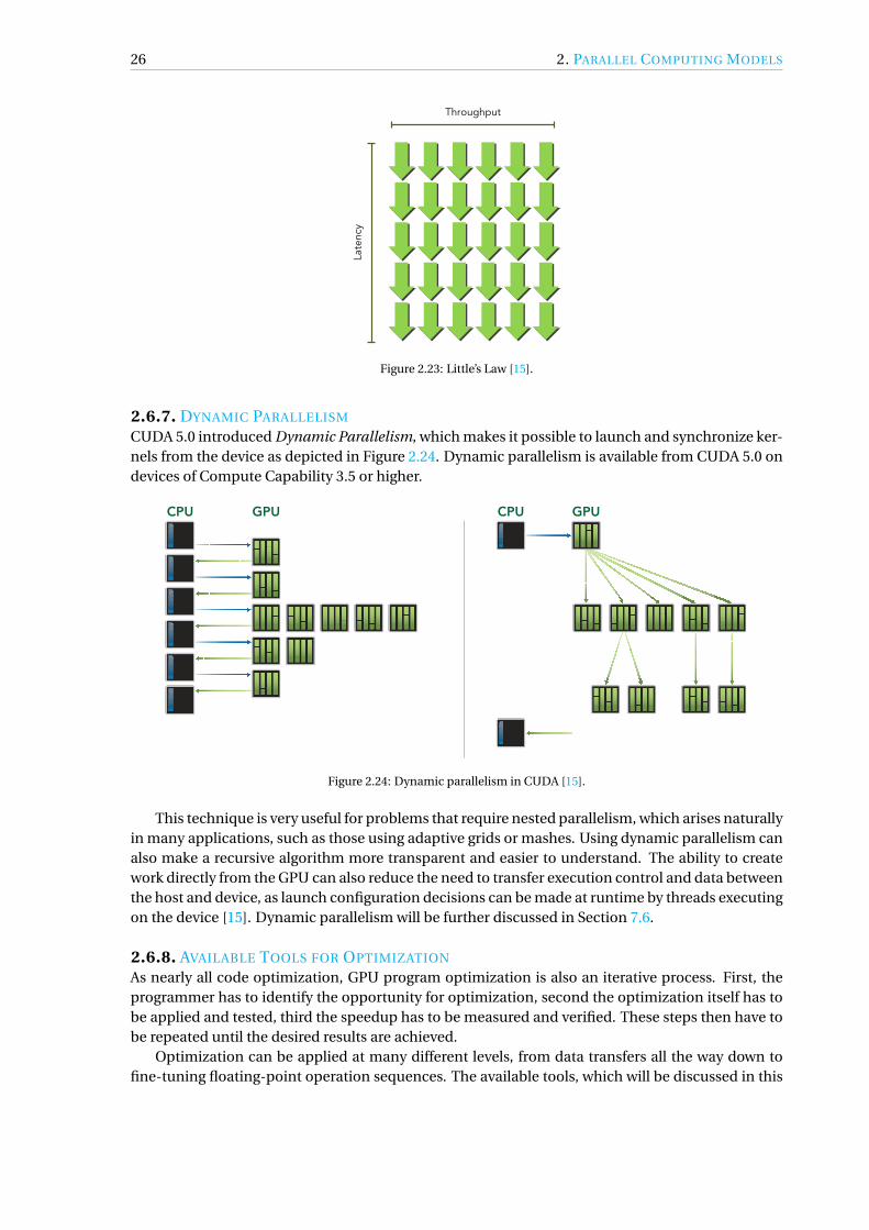
26 2. PARALLEL COMPUTING MODELS
Throughput
Late
ncy
Figure 2.23: Little’s Law [15].
2.6.7. DYNAMIC PARALLELISM
CUDA 5.0 introduced Dynamic Parallelism, which makes it possible to launch and synchronize ker-nels from the device as depicted in Figure 2.24. Dynamic parallelism is available from CUDA 5.0 ondevices of Compute Capability 3.5 or higher.
CPU GPU CPU GPU
Figure 2.24: Dynamic parallelism in CUDA [15].
This technique is very useful for problems that require nested parallelism, which arises naturallyin many applications, such as those using adaptive grids or mashes. Using dynamic parallelism canalso make a recursive algorithm more transparent and easier to understand. The ability to creatework directly from the GPU can also reduce the need to transfer execution control and data betweenthe host and device, as launch configuration decisions can be made at runtime by threads executingon the device [15]. Dynamic parallelism will be further discussed in Section 7.6.
2.6.8. AVAILABLE TOOLS FOR OPTIMIZATION
As nearly all code optimization, GPU program optimization is also an iterative process. First, theprogrammer has to identify the opportunity for optimization, second the optimization itself has tobe applied and tested, third the speedup has to be measured and verified. These steps then have tobe repeated until the desired results are achieved.
Optimization can be applied at many different levels, from data transfers all the way down tofine-tuning floating-point operation sequences. The available tools, which will be discussed in this
2.6. GPU PARALLELISM 27
section, are invaluable for helping this process, as they can suggest a next-best course of action forthe programmer’s optimization efforts.
CUDA-GDB COMMAND LINE DEBUGGER
A traditional CPU debugger is not capable of handling thousands of threads running simultane-ously on multiple devices, therefore NVIDIA developed its own debugger CUDA-GDB for debuggingCUDA code. CUDA-GDB is capable of debugging both the CPU and GPU portions of an applicationsimultaneously. CUDA-GDB is an extension to the classical GDB debugger, just as programmingin CUDA C is an extension to C programming. The existing GDB debugging features are inherentlypresent for debugging the host code, and additional features have been provided to support debug-ging CUDA device code. CUDA-GDB supports debugging C/C++ and Fortran CUDA applications.
This tool is currently available on Linux and Mac machines. Windows users have to use NVIDIANsight Visual Studio Edition for debugging and profiling CUDA code. The detailed documentationof CUDA-GDB can be found in [20].
CUDA-MEMCHECKMemory access errors are very common bugs in CUDA code, and accurately identifying the sourceand cause of these errors can be rather cumbersome. CUDA-MEMCHECK, which was developed byNVIDIA, contains multiple parts that can perform different types of checks.
The memcheck tool is capable of detecting and locating memory access errors in GPU code. Italso reports runtime execution errors, identifying situations that could otherwise result in an un-specified launch failure error. This tool can also be run in integrated mode inside CUDA-GDB.
The racecheck tool can report shared memory data access hazards that can cause data races.A data access hazard is a case where two threads attempt to access the same location in memoryresulting in nondeterministic behavior, based on the relative order of the two accesses.
The initcheck tool is a run time uninitialized device global memory access detector. This toolcan identify situations when device global memory is accessed without initialization.
The synccheck tool can report cases where the program is attempting invalid usages of synchro-nization primitives.
CUDA OCCUPANCY CALCULATOR
The CUDA Occupancy Calculator is a spreadsheet produced by NVIDA that allows to compute themaximum theoretical SM occupancy of a GPU by a given CUDA kernel. The SM occupancy is theratio of active warps to the maximum number of warps supported on an SM. A warp is consideredactive from the time its threads begin executing their instructions to the time when all the threadswithin that warp have finished their instructions. The maximum number of warps residing on an SMis currently 64 for all GPUs that have at least Compute Capability 3.0, which translates of a maximumof 32× 64 = 2048 threads on an SM. Note that the maximum number of resident blocks per SMchanges with different architectures.
Maximizing the occupancy can help to cover latency during global memory loads, howeverhigher occupancy does not necessarily mean higher performance, which will be shown in Section7.2.1. The occupancy is determined by the amount of shared memory and registers used by eachblock, therefore programmers need to choose the number of threads per block with care in order tomaximize occupancy.
After setting the Compute Capability and the maximum amount of available shared memory ofthe device, the user can set three kernel resource attributes in the occupancy calculator as shown inFigure 2.25:
• Threads per block• Registers per thread• Shared memory per block

28 2. PARALLEL COMPUTING MODELS
Maximum warps = 64
24 active warps means 38% occupancy
Figure 2.25: Occupancy calculator spreadsheet [16].
The threads-per-block attribute is set as one of the input arguments of the kernel launch and canbe any number between 1 and 1024. It is highly recommended to launch kernels with a threads-per-block number that is divisible by 32 since the number of threads within a warp is 32 for all devices.As a rule of thumb, 128 or 256 is usually a good number. In the specific example in Figure 2.25 thisvalue is 128.
Each SM on the GPU has a set of registers available for use by CUDA thread programs. Theseregisters are a shared resource that are allocated among the blocks executing on an SM. The CUDAcompiler attempts to minimize register usage to maximize the number of blocks that can be activeon the device simultaneously. It is possible to maximize the number of registers per thread withthe --maxrregcount flag of the nvcc compiler. The maximum number of registers per thread isdifferent for each GPU architecture. The number of registers per thread in the particular example inFigure 2.25 is 16.
The maximum amount of shared memory per SM changes with different architectures, howeverthe maximum amount of shared memory per block is 48 kB for all architectures except the Volta andTuring families, where it is 96 kB and 64 kB respectively. The shared memory used by each block is

2.6. GPU PARALLELISM 29
8 kB in the example in Figure 2.25. The registers per thread and shared memory per block resourceusage of any kernel can be obtained from nvcc’s --ptxas-options=-v compiler flag.
After the input has been set by the user, the occupancy calculator produces three plots whichshow the occupancy of the SM with the impact of varying the block size, shared memory per blockusage for a given block size, and register count per thread usage for a given block size, as shown inFigures 2.26, 2.27 and 2.28.
Figure 2.26: Impact of varying block size on multiprocessor warp occupancy [16].
Figure 2.27: Impact of varying shared memory usage per block on multiprocessor warp occupancy [16].
The pattern of the figures can be very diverse for GPUs with different Compute Capabilities andshared memory sizes and is determined by the resources that are associated with that ComputeCapability.
For the users the most important figure is the one that shows the impact of varying block sizeof a kernel, because it can be changed very easily without modifying the kernel itself. As shown inFigure 2.26, changing the block size from 128 to 1024 could increase the occupancy from 38% to100%.

30 2. PARALLEL COMPUTING MODELS
Figure 2.28: Impact of varying register count per thread on multiprocessor warp occupancy [16].
The occupancy calculator provides a summary of which one of the three resources will be ex-posed to the limitation before the others, as shown in Figure 2.29. In this specific case, the limitedamount of shared memory (48 kB) limits the total number of blocks that can be launched to 6. Al-ternatively, the number of registers or the maximum number of blocks per SM does not become alimitation, which is the reason that the occupancy is constant in Figure 2.28.
Figure 2.29: Resource limitation calculated by the Occupancy Calculator [16].
NVIDIA PROFILING TOOLS
There are two tools in the NVIDIA Profiling Tools package, which can be found in the CUDA Toolkit:the Visual Profiler and the nvprof profiling tool. The Visual Profiler is a graphical profiling toolthat displays a timeline of a CUDA application’s CPU and GPU activity. It includes an automatedand manual analysis engine to identify potential performance bottlenecks and optimization op-portunities. The nvprof profiling tool enables the user to collect and view profiling data from thecommand-line [19].
One of the view modes in the Visual Profiler is the timeline view shown in Figure 2.30 in whichthe user can check the activity of a CUDA application occuring on both CPU and GPU in a uni-fied time line. The activities include CUDA API function calls, memory transfers and CUDA ker-nel launches. Performance metrics such as cache hit rates, memory throughput, branch efficiency,etc. can be collected directly from GPU hardware counters and software instrumentation to gainlow-level insight of an application. Performance improvements can be compared against previous

2.7. CONCLUSIONS 31
versions of any application. The Visual Profiler also supports CUDA dynamic parallelism, there-fore both host-launched and device-launched kernels and the relationship between them can beinvestigated. The guided analysis mode is capable of providing the user a step-by-step analysis andoptimization guidance. Additionally, GPU power, thermal and clock values can be observed duringapplication execution.
Figure 2.30: Timeline view of the NVIDIA Visual Profiler [19].
The nvprof command line profiling tool has similar capabilities to the Visual Profiler without thegraphical interface. The user can set different modes such as the summary mode, the GPU-Tracemode or the Event/metric mode. Profiling results are displayed in the console after the profilingdata is collected, and may also be saved for later viewing by either nvprof or the Visual Profiler. Thedetailed description of the NVIDIA Profiling tools can be found in [19].
2.7. CONCLUSIONSIn this chapter, an introduction to parallel computing was presented with the key focus on GPU par-allelism. Considering the physical limitations of the development of traditional serial processors itwas inevitable that parallelism had to be incorporated in hardware design. Designers utilize differ-ent types of parallelism in their new architectures which can be categorized using Flynn’s Taxonomy.
Modern CPUs are designed as multi-core, multi-thread processors, which are capable of paral-lel computations. However, for applications that can exploit data parallelism using thousands ormillions of threads, even a modern CPU reaches its limitations. Therefore, GPUs were inventedwhich contain thousands of processors and are designed for maximizing throughput. Traditionally,all GPUs were designed for graphical applications, however from the mid 2000s onwards vendorsstarted to develop GPGPUs which can be used for massively parallelized scientific calculations.
The CUDA programming language is a great choice for GPGPU programming, because it is veryrobust and has many features such as its own debugger or dynamic parallelism which make CUDAapplications widely applicable for scientific and astrodynamics problems. Because the architectureof modern NVIDIA GPUs is constantly changing, it is an accepted practice to develop and optimizea CUDA application for a selected architecture; however some features are common for every GPU.
GPGPU programmers should limit CPU–GPU data transfers in their code, because the band-width of the PCIe bus, which is the connection between the CPU and the GPU, is much smaller thanthe bandwidth of the global memory of the GPU. Developers should pay attention to avoid warp di-vergence and exploit the latency hiding effect of GPUs as much as possible. Sophisticated memoryusage and choosing the optimal thread hierarchy are also extremely important to develop efficientapplications. Optimization tools such as the CUDA Occupancy Calculator and the NVIDIA Profilercan help developers to improve their code to achieve better performance.

3 ENVIRONMENTAL MODELS
In this chapter, the implemented environmental models and algorithms are described which will beused by the test and study cases presented in the following chapters. After a brief introduction ofreference frames and frame transformations, the used force models will be described. At the end ofthe chapter the used ephemeris model will be discussed in more detail.
3.1. REFERENCE FRAMESFor determining the position and velocity of a spacecraft at a certain moment of time, a referenceframe, with respect to which position and velocity are described, is required. Usually referenceframes are categorized into two main types: inertial or pseudo-inertial and non-inertial referenceframes. A reference system on the other hand is a set of physical definitions and models whichideally define a celestial coordinate system. It is also commonly said that a reference frame is thepractical realization of a reference system [21].
3.1.1. INERTIAL REFERENCE FRAMES
The formal definition of an inertial reference frame can be derived from Newton’s first law: “Aninertial reference frame is a reference frame with respect to which a particle remains at rest or inuniform rectilinear motion if no resultant force acts upon that particle [21].”
ICRF
One of the most commonly used celestial reference system for astrodynamics applications is theInternational Celestial Reference System (ICRS), which is a space-time coordinate system withinthe framework of general relativity theory, with its origin at the Solar System barycenter and its axesdirections fixed with respect to distant quasars and active galactic nuclei. The realization of thisreference system is the International Celestial Reference Frame (ICRF).
This system and frame are meant to represent the most appropriate coordinate system currentlyavailable for expressing reference data on the positions and motions of celestial or man-made ob-jects. Its z-axis is defined by the principal plane which has to be "close to the mean equator atJ2000.0 epoch (1st January 2000 at 12.0h, or Julian Date 2451545.0)" according to the InternationalEarth Rotation and Reference Systems Service (IERS). Its x-axis also defined by the IERS has to be"close to the dynamical equinox at J2000.0 epoch", which is the intersection of the celestial equatorand the solar ecliptic [22]. The y-axis is given by completing the orthonormal trihedron (y = z ×x).
Furthermore, since the defining radio sources are assumed to be so distant that their angularmotions, seen from Earth, are negligible, there is no epoch associated with the ICRF [21]. Addition-ally, because the distance from the planets to the Solar System barycenter is negligible comparedto the distance to the frame defining quasar radio sources, no rotation is needed to translate thissystem towards another body-centered e.g. Earth-centred definition.
J2000
The J2000 reference frame, which is also called EME2000, is based on distant stars rather thanquasars, therefore there is a very small difference (in the level of milliarcseconds) between them.For this reason, in many applications these two reference frames are considered to be equivalent.Note that in the SPICE toolkit the J2000 and the ICRF reference frames are also equivalent [23]. Themain difference between this system and the ICRS is that the J2000 frame is defined with an associ-ated epoch namely the J2000.0 epoch. The Earth-centered version of the J2000 frame is often calledas Earth Centered Inertial (ECI) frame.
33

34 3. ENVIRONMENTAL MODELS
3.1.2. NON-INERTIAL REFERENCE FRAMES
ITRFIn non-inertial reference frames accelerations are acting on them, therefore apparent forces arepresent in the system. One of the most commonly used non-inertial reference systems is the Inter-national Terrestrial Reference System (ITRS), which is a definiton of an Earth-fixed Earth-centeredsystem. Its realization is the International Terrestrial Reference Frame (ITRF), or the Earth CentredEarth Fixed (ECEF) frame. Its origin is placed in the center of mass of Earth. Its x-axis is point-ing towards the Greenwich Meridian, which is 0 in Earth coordinates. Its z-axis is directed alongthe mean pole of Earth’s rotation. Its y-axis is directed to complete the right-handed orthonormaltrihedron.
The transformation between this frame and the ICRF can be accomplished by using models forprecession, nutation, Earth rotation, and polar motion. The detailed description of these modelscan be found in [24].
3.1.3. FRAME TRANSFORMATIONS
The transformation between two reference frames can be done by applying a translation and a ro-tation. If the origin of the two frames is the same then only the rotation is necessary. For planetsand satellites the origin of its reference frames is usually the barycenter of the body, therefore totransform between inertial and body-fixed frames, only a rotation is required. The rotation can bedone by using several methods such as Euler angles, quaternions, etc. The IAU Working Group hasdefined planetary coordinate systems relative to their mean axis of rotation and various definitionsof longitude depending on the body (e.g. references to a surface feature such as a crater) [25].
The three rotational angles (90+α0,90−δ0,W ) that determine the transformation between abody-fixed frame and the ICRF can be seen in Figure 3.1.
North pole of body
Equatorof body
ICRF equator
B
Prime
m
eridian
(α0, δ
0)
ϒ
90˚- δ0Q
W
90+α
0
Figure 3.1: Reference system used to define orientation of the planets and their satellites [25].
The north pole is defined as the pole of rotation that lies on the north side of the invariableplane of the Solar System. The position of the north pole is given by the value of its right ascensionα0 and declination δ0. The two intersection points of the body’s equator and the ICRF equator areα0±90. α0+90 was chosen to define node Q as one of the intersection points. Point B was chosenas the intersection of the body’s prime meridian and equator. The location of the prime meridian isspecified by providing a value for W , which is the angle measured easterly along the body’s equatorbetween node Q and point B . The right ascension of the point Q is α0 +90 and the inclination ofthe planet’s equator to the celestial equator is 90−δ0 [25]. The constants (α0,δ0,W ) are given for
3.2. DYNAMICAL MODEL 35
each planet and their satellites in the form of polynomials at epoch J2000.0 Barycentric DynamicalTime (TDB).
The rotation between the position vector in the ICRF rIC RF and the body-fixed position vectorrb f can be written in a form of rotation matrices as follows [24]:
rb f =U (t )rIC RF (3.1)
where U (t ) is the time-dependent rotation matrix which has the following form:
U (t ) =u11 u12 u13
u21 u22 u23
u31 u32 u33
(3.2)
where
u11 = cosψcosφ−cosθ sinφsinψ
u12 = cosψsinφ+cosθcosφsinψ
u13 = sinψsinθ
u21 =−sinψcosφ−cosθ sinφcosψ
u22 =−sinψsinφ+cosθcosφcosψ
u23 = cosψsinθ
u31 = sinθ sinφ
u32 =−sinθcosφ
u33 = cosθ
(3.3)
where
φ= 90+α0
θ = 90−δ0
ψ=W
(3.4)
The rotation between the acceleration vector in the body-fixed frame ab f and acceleration inthe ICRF aIC RF is the following:
aIC RF =U T (t )ab f (3.5)
It will be shown later that these transformations are necessary to calculate the acceleration causedby the irregular gravity field of a celestial body.
3.2. DYNAMICAL MODELThe Equations of Motion (EOM) are a set of differential equations which describe the behaviour ofthe state vector x over time. There are several coordinate sets for which they can be described. Twoof the more common ones are Cartesian and Keplerian forms:
xC ar tesi an = (x, z, y, vx , vy , vz )T (3.6)
xK epler i an = (a,e, i ,ω,Ω,θ)T (3.7)

36 3. ENVIRONMENTAL MODELS
where x, z, y are the Cartesian position, vx , vy , vz are the Cartesian velocity coordinates of the space-craft, a is the semi-major axis, e is the eccentricity, i is the inclination,ω is the argument of pericen-ter,Ω is the right ascension of the ascending node and θ is the true anomaly of the trajectory.
The state vector can be extended by other parameters of the spacecraft such as mass, cross-sectional area, etc. In this case the equations of motion is extended by additional differential equa-tions for the time derivative of these parameters.
This section will describe the EOM in Cartesian frame as a set of second-order differential equa-tions. This can be done because the last three parameters (velocity) of the state vector are the timederivatives of the first three parameters (position). In a general form the equations in Cartesiancoordinates are the following:
a = d2r
dt 2 = r = F
m(3.8)
where a is the acceleration, r = (x, y, z)T is the position vector, F is the net external force on the bodyand m is its instantaneous mass. This form is only valid for inertial reference frames such as theICRF where no apparent forces appear.
If the motion of the satellite is expressed with respect to the barycenter of the system then theclassical n-body formulation describes the acceleration of the satellite, which is visualized in Figure3.2, where BC denotes the barycenter of the system, S/C denotes the satellite, and the dots representcelestial bodies that are part of the system.
𝑥𝑥
𝑦𝑦
𝑧𝑧
BC
𝒓𝒓𝑏𝑏𝑏𝑏𝒓𝒓𝑖𝑖
𝒓𝒓𝑖𝑖 − 𝒓𝒓𝑏𝑏𝑏𝑏𝑖𝑖
S/C
Figure 3.2: Barycentric formulation of the n-body problem.
The barycentric form of the EOM is the following:
rbc =n∑
i=1µi
ri − rbc
|ri − rbc |3(3.9)
where the subscript bc denotes satellite’s coordinates with respect to the barycenter, n is the numberof celestial bodies considered in the equations, µi is the gravitational parameter of celestial body iand ri is the position vector with respect to the barycenter of body i . Note that this formulation isonly valid if all the bodies with non-negligible masses are considered in the equations. However inmost applications the center of propagation is not the barycenter of the system but a real physicalbody, therefore another formulation is used to express the motion of the satellite.

3.2. DYNAMICAL MODEL 37
In the unperturbed case only the gravitational force of the central body is present. The EOM hasthe following form:
r =− µ
r 3 r =−∇U =−∂U
∂r(3.10)
where µ is the gravitational parameter of the central body and r = |r|. This equation can also beobtained using the negative gradient of a scalar potential:
U =−µr
(3.11)
where U is the potential.In the perturbed case not only the acceleration of the central body as a point mass is taken into
account but other perturbing forces that act upon the spacecraft are included as well. This can beexpressed in the following form:
r =− µ
r 3 r+ f (3.12)
where f is the acceleration induced by the perturbing forces. The following section will describepossible contributions to f which are implemented in the software.
3.2.1. GRAVITY MODEL
SPHERICAL HARMONICS
This perturbation arises from the irregular mass distribution of a celestial body, which can be ex-pressed as spherical harmonic expansion of the potential. The potential has the following form:
U (r,φ,λ) =−µr
∞∑n=0
n∑m=0
(R
r
)n
Pnm(sinφ) (Snm sin(mλ)+Cnm cos(mλ)) (3.13)
where r is the distance from the body center to the satellite, φ is the geocentric latitude, λ is the eastlongitude measured from the reference meridian, R is the equatorial radius of the central body, Pnm
are the associated Legendre polynomials, Snm , Cnm are spherical harmonics coefficients and n isthe degree, m is the order of the spherical harmonics. Some of the lower-order associated Legendrepolynomials can be found explicitly in Table 3.1.
Table 3.1: Associated Legendre polynomials up to degree and order two [24].
n m Pnm(sinφ)0 0 11 0 sinφ1 1 cosφ2 0 1
2 (3sin2φ−1)2 1 3sinφcosφ2 2 3cos2φ
Since the values of the spherical harmonics coefficients cover a large range of ten or more ordersof magnitude, usually the normalized coefficients Snm and Cnm are given, which are defined asfollows:
38 3. ENVIRONMENTAL MODELS
Snm =√
(n +m)!
(2−δ0m)(2n +1)(n −m)!Snm (3.14)
Cnm =√
(n +m)!
(2−δ0m)(2n +1)(n −m)!Cnm (3.15)
where δnm is the Kronecker delta, which is defined as follows:
δnm =
1, if n = m
0, if n 6= m(3.16)
In case of using normalized coefficients, the associated Legendre polynomials also have to be nor-malized as follows:
Pnm =√
(2−δ0m)(2n +1)(n −m)!
(n +m)!Pnm (3.17)
where Pnm is called the normalized associated Legendre polynomial. The EOM of the perturbedorbit can be obtained by calculating the gradient of the potential given by Eq. (3.13), which alsocontains the unperturbed part (n = m = 0):
r =−∇U =−∂U
∂r(3.18)
The calculation of these derivatives can be done using recursive algorithms such as the Cun-ningham algorithm. The potential U can also be defined in the following form [24]:
U =−µR
∞∑n=0
n∑m=0
(SnmWnm +CnmVnm) (3.19)
where Vnm and Wnm are as follows:
Vnm =(
R
r
)n+1
·Pnm(sinφ) ·cos(mλ) (3.20)
Wnm =(
R
r
)n+1
·Pnm(sinφ) · sin(mλ) (3.21)
The coefficients for any n,m can be calculated using the following two relations [24]:
Vmm = (2m −1)
(xR
r 2 Vm−1,m−1 − yR
r 2 Wm−1,m−1
)(3.22)
Wmm = (2m −1)
(xR
r 2 Vm−1,m−1 + yR
r 2 Wm−1,m−1
)(3.23)
Vnm =(
2n −1
n −m
)zR
r 2 Vn−1,m −(
n +m −1
n −m
)R2
r 2 Vn−2,m (3.24)
Wnm =(
2n −1
n −m
)zR
r 2 Wn−1,m −(
n +m −1
n −m
)R2
r 2 Wn−2,m (3.25)

3.2. DYNAMICAL MODEL 39
where x, y, z are Cartesian position coordinates in the body-fixed frame and V00 = Rr , W00 = 0. The
acceleration r = (x, y , z) in the body-fixed frame can be calculated as the sum of partial accelerationswhich correspond to each of the harmonic components as follows:
x = ∑n,m
xnm
y = ∑n,m
ynm
z = ∑n,m
znm
(3.26)
where the partial accelerations xnm , ynm , znm are the following [24]:
xnm =
µ
R2
(−Cn0Vn+1,1)
, if m = 0
µ
2R2
((−CnmVn+1,m+1 −SnmWn+1,m+1)
+ (n −m +2)!
(n −m)!
(CnmVn+1,m−1 +SnmWn+1,m−1
)), if m > 0
ynm =
µ
R2
(−Cn0Wn+1,1)
, if m = 0
µ
2R2
((−CnmWn+1,m+1 −SnmVn+1,m+1)
+ (n −m +2)!
(n −m)!
(CnmWn+1,m−1 +SnmVn+1,m−1
)), if m > 0
znm = µ
R2
((n −m +1)
(−CnmVn+1,m −SnmWn+1,m))
(3.27)
It can be seen from the formulas that the Vnm and Wnm terms have to be calculated up to degreeand order n+1, m+1 if the potential coefficients are calculated up to n and m. After the calculationof the accelerations, a coordinate transformation is required, using Eq. (3.5), to obtain the inertialaccelerations which will be consistent with the EOM [24].
J2 PERTURBATION
The spherical harmonics expansion of the potential (Eq. (3.13)) can also be expressed in a differentform [21]:
U (r,φ,λ) =−µr
(1−
∞∑n=2
Jn
(R
r
)n
Pn(sinφ)+∞∑
n=2
n∑m=1
Jn,m
(R
r
)n
Pnm(sinφ)(cos(m(λ−Λn,m))
))(3.28)
where Jn =−Cn0, Pn(sinφ) = Pn0(sinφ), Jnm =√
C 2nm +S2
nm , andΛnm = 1m arctan
(SnmCnm
). The J2 term
has a special importance because it reflects to the oblateness of the central body and usually has thelargest contribution after the point-mass term in the spherical harmonics expansion. The J2 termof the potential in Cartesian coordinates can be described as follows [21]:
UJ2 =1
2µJ2
R2
r 3
(3
z2
r 2 −1
)(3.29)
The corresponding accelerations after evaluating the derivatives of the potential are the following:
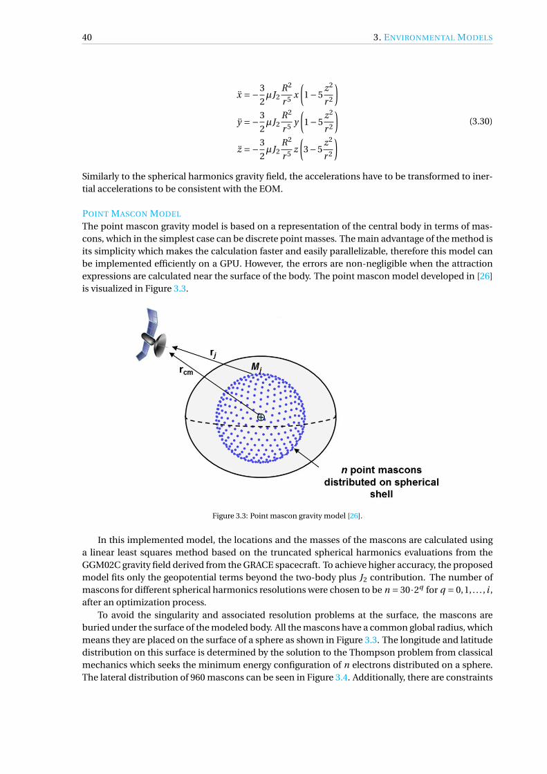
40 3. ENVIRONMENTAL MODELS
x =−3
2µJ2
R2
r 5 x
(1−5
z2
r 2
)y =−3
2µJ2
R2
r 5 y
(1−5
z2
r 2
)z =−3
2µJ2
R2
r 5 z
(3−5
z2
r 2
) (3.30)
Similarly to the spherical harmonics gravity field, the accelerations have to be transformed to iner-tial accelerations to be consistent with the EOM.
POINT MASCON MODEL
The point mascon gravity model is based on a representation of the central body in terms of mas-cons, which in the simplest case can be discrete point masses. The main advantage of the method isits simplicity which makes the calculation faster and easily parallelizable, therefore this model canbe implemented efficiently on a GPU. However, the errors are non-negligible when the attractionexpressions are calculated near the surface of the body. The point mascon model developed in [26]is visualized in Figure 3.3.
Figure 3.3: Point mascon gravity model [26].
In this implemented model, the locations and the masses of the mascons are calculated usinga linear least squares method based on the truncated spherical harmonics evaluations from theGGM02C gravity field derived from the GRACE spacecraft. To achieve higher accuracy, the proposedmodel fits only the geopotential terms beyond the two-body plus J2 contribution. The number ofmascons for different spherical harmonics resolutions were chosen to be n = 30·2q for q = 0,1, . . . , i ,after an optimization process.
To avoid the singularity and associated resolution problems at the surface, the mascons areburied under the surface of the modeled body. All the mascons have a common global radius, whichmeans they are placed on the surface of a sphere as shown in Figure 3.3. The longitude and latitudedistribution on this surface is determined by the solution to the Thompson problem from classicalmechanics which seeks the minimum energy configuration of n electrons distributed on a sphere.The lateral distribution of 960 mascons can be seen in Figure 3.4. Additionally, there are constraints

3.2. DYNAMICAL MODEL 41
on the total mass and total dipole moment of the mascons, which both set to be zero, because thepoint mass representation of the body in the expression of the potential (leading term in Eq. (3.31))already considers the total mass of the body and the true surface integral of the spherical harmonicsfitting function evaluated over the full surface is zero [26].
Figure 3.4: Lateral distribution of the mascons based on the converged solution of the Thompson problem (n = 960) [26].
The total potential in the point mascon model is the following:
U (r) =−µr
(1− J2
(R
r
)2 (3z2
2r 2 − 1
2
)+
n∑j=1
µ j
|ρ j − r|
)(3.31)
where n is the number of mascons, µ j is the gravitational potential of each mascon, and ρ j is thelocation of each mascon. The accelerations are simply the sum of the derivatives of the individualterms which can be found in Eqs. (3.10) and (3.30).
The detailed procedure using the linear least squares method to calculate the µ j and ρ j param-eters can be found in [26]. Note that multiple solutions with different number of mascons for Earthare provided in [27].
3.2.2. THIRD-BODY PERTURBATION
Third-body perturbations are modeled as point mass forces, which can be described in the followingequation [24]:
r =µp
(rp − r
|rp − r|3 − rp
|rp |3)
(3.32)
where µp is the gravitational parameter of the perturbing body, and rp is the inertial position vectorof the perturbing body. The first term in this expression is the so-called direct or principal part andthe second term is the indirect part of the total acceleration. The position vector of the perturb-ing body is usually given by ephemerides such as JPL ephemeris model which will be described inSection 3.3.
3.2.3. SOLAR RADIATION PRESSURE
The Solar Radiation Pressure (SRP) is due to the momentum transfer of photons emitted by the Sunand hitting the exposed surface of an orbiting spacecraft. This perturbation is modeled using thefollowing equation [24]:
r = νP¯AU2CrAr
m
r− r¯|r− r¯|3 (3.33)
where ν is the shadow factor, P¯ = 4.56 ·10−6 N/m2 is the force due to SRP at one astronomical unit(AU) and on unit area, AU = 1.49597870700 · 109 m is the astronomical unit, Cr is the reflectivity

42 3. ENVIRONMENTAL MODELS
coefficient of the spacecraft, Ar is the area exposed to the Sun’s direction, m is the mass of thespacecraft and r¯ is the inertial position vector of the Sun. The shadow factor can be determinedby the eclipse conditions as follows:
ν=
0, umbra (total eclipse)
1, sunlight
0 < ν< 1, penumbra (partial eclipse), annular eclipse
(3.34)
Eclipse conditions can be determined by the dual cone shadow model, which can be seen inFigure 3.5. This model assumes a finite size and distance of the Sun creating the penumbra andumbra regions in the occulting body’s shadow.
SunOcculting body
Umbra
Penumbra
Penumbra
Sunlight
Sunlight
Satellite orbit
Total eclipse
Partial eclipse
Annular eclipse
Partial eclipse
Figure 3.5: Dual cone shadow model with different lighting conditions for a satellite.
The geometry of the Sun and the occulting body from the satellite’s point of view and the vari-ables to calculate the shadow factor can be seen in Figure 3.6.
Sun Occulting body
𝑅𝑅ʘ
𝑅𝑅𝑏𝑏
𝒓𝒓𝑏𝑏 − 𝒓𝒓𝒓𝒓ʘ − 𝒓𝒓
Spacecraft
𝑎𝑎𝑏𝑏
𝑐𝑐
Figure 3.6: Eclipse geometry and variables to calculate the shadow factor.
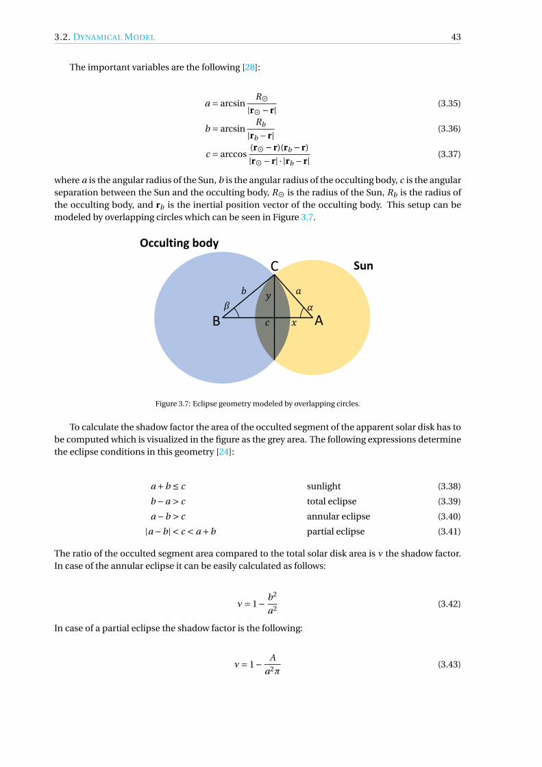
3.2. DYNAMICAL MODEL 43
The important variables are the following [28]:
a = arcsinR¯
|r¯− r| (3.35)
b = arcsinRb
|rb − r| (3.36)
c = arccos(r¯− r)(rb − r)
|r¯− r| · |rb − r| (3.37)
where a is the angular radius of the Sun, b is the angular radius of the occulting body, c is the angularseparation between the Sun and the occulting body, R¯ is the radius of the Sun, Rb is the radius ofthe occulting body, and rb is the inertial position vector of the occulting body. This setup can bemodeled by overlapping circles which can be seen in Figure 3.7.
Occulting body
Sun
𝑎𝑎𝑏𝑏
𝑐𝑐
𝑦𝑦
𝑥𝑥𝛽𝛽 𝛼𝛼
AB
C
Figure 3.7: Eclipse geometry modeled by overlapping circles.
To calculate the shadow factor the area of the occulted segment of the apparent solar disk has tobe computed which is visualized in the figure as the grey area. The following expressions determinethe eclipse conditions in this geometry [24]:
a +b ≤ c sunlight (3.38)
b −a > c total eclipse (3.39)
a −b > c annular eclipse (3.40)
|a −b| < c < a +b partial eclipse (3.41)
The ratio of the occulted segment area compared to the total solar disk area is ν the shadow factor.In case of the annular eclipse it can be easily calculated as follows:
ν= 1− b2
a2 (3.42)
In case of a partial eclipse the shadow factor is the following:
ν= 1− A
a2π(3.43)

44 3. ENVIRONMENTAL MODELS
where A the occulted area can be expressed as follows [24]:
A = a2α+b2β− c · y (3.44)
where the two angles α and β as well as the segments x and y are the following:
α= arccosx
a(3.45)
β= arccosc −x
b(3.46)
x = c2 +a2 −b2
2c(3.47)
y =√
a2 −x2 (3.48)
3.3. JPL EPHEMERIS MODELThe Jet Propulsion Laboratory (JPL) provides high-precision numerically integrated planetary andlunar ephemerides called Development Ephemerides (DE) to support spacecraft missions and otheractivities relating to Solar System bodies. The detailed description of the different ephemeris filescan be found in [29]. The bodies that can be found in the files are: Mercury, Venus, Earth-Moonbarycenter, Mars, Jupiter, Saturn, Uranus, Neptune, Pluto, Moon, Sun. Some of the files also con-tain information about nutation angles and lunar libration angles as well as lunar mantle angularvelocities and the difference between Terrestrial Time (TT) and Barycentric Dynamical Time (TDB).
JPL also provides an open-source toolkit for reading the files called the SPICE toolkit [23]. Notethat this toolkit is not available for GPUs. Usually the files do not contain the states of the integratedbodies. Instead, the JPL planetary ephemerides are saved as sets of Chebyshev polynomials fit tothe Cartesian positions and velocities of the celestial bodies, typically in 32-day intervals. The nthChebyshev polynomial can be defined by the following recursion formula [30]:
Tn(τ) = 2τTn−1(τ)−Tn−2(τ), n = 2,3, . . . (3.49)
where Tn(τ) is the nth Chebyshev polynomial with T0(τ) = 1 and T1(τ) = τ. The interval of themapped time τ for interpolation is −1 < τ ≤ 1. The mapping transformation from a finite timeinterval [t1, t2] to [−1,+1] can be performed by the following transformation [24]:
τ= 2t − t1
t2 − t1−1 (3.50)
where t is an arbitrary epoch. The Chebyshev approximation of a given function f is the following:
f (t ) ≈N∑
n=0anTn(τ) (3.51)
where an are coefficients which serve to define the function f (t ) and can be calculated from thenumerically integrated position and velocity coordinates described in [30]. Using these coefficientsthe calculated f (t ) and f (t ) functions (position and velocity) are an exact fit to the boundaries ofthe interval [t1, t2] and a least-squares fit to the interior points.
As mentioned before, the complete ephemeris is blocked into data records, where each recordcovers typically 32 days and contains the Chebyshev polynomial coefficients of the positions of theaforementioned eleven Solar System bodies and optionally the orientation angles and TT-TDB. It is

3.3. JPL EPHEMERIS MODEL 45
possible that within one record the time covered by each polynomial is smaller than the interval ofthe whole record due to the large difference in the period of the Solar System bodies. The structureof the records can be seen in Table 3.2.
Table 3.2: Structure of the JPL ephemeris records.
begin end bodyi . . . body j
t1 t2 x11 . . . xnk y11 . . . ynk z11 . . . znk . . . x11 . . . xn1 y11 . . . yn1 z11 . . . zn1
t2 t3 x11 . . . xnk y11 . . . ynk z11 . . . znk . . . x11 . . . xn1 y11 . . . yn1 z11 . . . zn1
The beginning and end of the time intervals that the record covers is denoted by ti . To makethe data consistent and continuous the end times of the records have to be equal to the beginningtimes of the next record. The an coefficients from Eq. (3.51) for the position coordinates are denotedby xnk , ynk , znk , where n is the number of Chebyshev coefficients for the given body and k is thenumber of sub-intervals within the record. It can be seen that in this particular example the j thbody has only one sub-interval.
The evaluation of the polynomials yields Cartesian coordinates in km for the planets, Pluto,the Earth-Moon barycenter and the Sun with respect to the Solar System barycenter, while lunarpositions are given with respect to the center of Earth. To calculate the position of Earth or Moonwith respect to the Solar System barycenter, the barycentric formulas and the mass ratio of Earthand Moon has to be considered. The mass ratio can usually be retrieved from the header of the DEfiles. The nutations and librations are stored in radians, the mantle angular velocities are stored inradians/day, and the TT-TDB is stored in seconds.
Table 3.3 summarizes the number of Chebyshev coefficients n and sub-intervals k and the sizesof the sub-intervals ∆t for different ephemerides. It can be seen that the time covered by eachpolynomial has been chosen in accordance with the period of revolution of the individual bodies.
Table 3.3: Data contained in different Development Ephemerides files (EMB denotes Earth-Moon barycenter).
DE200 DE405 DE406 DE422 DE430t# Body n k ∆t n k ∆t n k ∆t n k ∆t n k ∆t1 Mercury 12 4 8 14 4 8 14 4 16 14 4 8 14 4 82 Venus 12 1 32 10 2 16 12 1 64 10 2 16 10 2 163 EMB 15 2 16 13 2 16 9 2 32 13 2 16 13 2 164 Mars 10 1 32 11 1 32 10 1 64 11 1 32 11 1 325 Jupiter 9 1 32 8 1 32 6 1 64 8 1 32 8 1 326 Saturn 8 1 32 7 1 32 6 1 64 7 1 32 7 1 327 Uranus 8 1 32 6 1 32 6 1 64 6 1 32 6 1 328 Neptune 6 1 32 6 1 32 6 1 64 6 1 32 6 1 329 Pluto 6 1 32 6 1 32 6 1 64 6 1 32 6 1 32
10 Moon 12 8 4 13 8 4 13 8 8 13 8 4 13 8 411 Sun 15 1 32 11 2 16 12 1 64 11 2 16 11 2 1612 Nutation 10 4 8 10 4 8 10 4 813 Libration 10 4 8 10 4 8 10 4 814 Ang.vel.15 TT-TDB 11 4 8

4 PROPAGATION
This chapter will briefly describe the used propagation and integration techniques which are imple-mented in the software.
4.1. COWELL’S METHODCowell’s method is one of the three classical special perturbations methods to propagate a trajectoryfor given specific initial conditions. The computation of the orbit is done by a numerical integrationprocess. Other commonly used methods are Encke’s method or the method of variation of orbitalelements.
Cowell’s method is the simplest, most straightforward formulation of the computation of per-turbed orbits which has the following form [21]:
r =− µ
r 3 r−∇R + f (4.1)
where R is the perturbing potential, and f contains all the perturbing forces that cannot be written asa gradient of a potential function. For most cases this formulation is sufficient to calculate perturbedorbits, however it does not make use of the fact that ∇R and f are perturbing forces [21].
4.2. NUMERICAL INTEGRATION WITH RUNGE–KUTTA METHODSNumerical integrators are a wide family of algorithms that are used to find numerical approxima-tions to the solutions of ODEs. They are based on the concept of quadrature and try to approximatethe analytical solution with a consecution of grid points that are calculated for every step of the in-tegration. The number of steps to be taken determines the accuracy of the integration, as well as thecomputational time that it takes.
There are several categories of numerical integrators such as fixed step size, variable step size,single-step, multi-step, implicit, explicit, extrapolation, etc. In this document only single-step inte-grators will be described. In a single-step method all integration steps are calculated independentlyfrom each other. Some of the most famous single-step numerical methods are the Euler methodand the Runge–Kutta (RK) methods, which all work with first-order ODEs. In this document thegeneral RK method and the Runge–Kutta–Fehlberg 7(8) (RKF78) integrator will be described as anexample because this integrator is implemented in the software.
The family of RK methods arises from the extension of the Euler method. The RK methods arebased on the discretization of the step to be taken in a number of stages; for each one an evaluationof the derivative is made. This process results in a higher number of evaluations than the simple Eu-ler method which causes longer computational time, but it highly improves the numerical accuracy.The general RK method is meant to find the solution of the following first-order ODE:
x(t ) = f (t ,x(t )) (4.2)
with
x(t0) = x0 (4.3)
where f is an arbitrary function, x is an unknown scalar or vector, t0 is the initial time and x0 is theinitial value of x at t0.
47
48 4. PROPAGATION
4.2.1. FIXED TIME STEP
Fixed time step methods use a constant time step throughout the integration. This is a simple butnot optimal method, especially for integrating elliptical orbits where the velocity of the satellite ischanging significantly. The fixed time step RK method of order q , which is often noted as RKq , hasthe following form [31]:
xn+1 = xn +hs∑
i=1bi ki (4.4)
ki = f
(tn + ci h, yn +h
i−1∑j=1
ai j k j
), i = 1, . . . , s (4.5)
where n is the actual step number, s is the number of function evaluations or stages, h = tn+1 − tn
is the step size, ai j ,bi ,ci are constants. The latter constants can be found in the so-called Butchertableaus. The constants ai j and ci always have to satisfy the following condition:
ci =i−1∑j=0
ai j (4.6)
4.2.2. VARIABLE TIME STEP
Variable time step integrators use different step sizes to optimize their performance. Usually twosets of solutions are calculated with different orders (using different values for the constants a,b,c),and the difference of these solutions is then used to calculate the next time step. These two solu-tions are often called Runge–Kutta discrete embedded pairs and noted as RKq(p) where q > p formethods that use local extrapolation. A general example of an Runge–Kutta embedded pair can beseen below [31]:
xn+1 = xn +hn
s∑i=1
bi ki (4.7)
xn+1 = xn +hn
s∑i=1
bi ki (4.8)
ki = f
(tn + ci hn , yn +hn
i−1∑j=1
ai j k j
), i = 1, . . . , s∗ (4.9)
where n is the actual step number, s, s∗ are the number of function evaluations or stages (usuallys∗ ≥ s), hn = tn+1 − tn is the actual step size, ai j , bi ,bi ,ci are constants where Eq. (4.6) also holds.
The Butcher tableau of the RKF78 method, which also can be denoted as RK7(8) using the afore-mentioned notation, is tabulated in Table 4.1.
It can be seen that RKF78 uses eleven function evaluations to calculate the 7th-order solution,and two extra function evaluations for a total of thirteen for controlling the step size. The localtruncation error of the RKF78 method is O (h8).
The Fehlberg method propagates the integration from the lower-order approximation by xn tothe true solution x(tn) and uses the higher-order solution xn only to control the step size. This isin accordance to other embedded methods such as the Dormand–Prince method, which uses theso-called local extrapolation. In local extrapolation mode the integration is propagated from thehigher-order approximation by xn to the true solution x(tn) and the lower-order discrete process xn
is used for step size control.The values of ci will have a special importance in the optimization of the ephemeris retrieval,
which will be explained in Section 7.5.

4.2. NUMERICAL INTEGRATION WITH RUNGE–KUTTA METHODS 49
Table 4.1: The Butcher tableau of the RKF78 method (s = 13) [31].
ci ai j bi bi
0 0 41840 0
227
227 0 0
19
136
112 0 0
16
124 0 1
8 0 05
125
12 0 − 2516
2516 0 0
12
120 0 0 1
415
34105
34105
56 − 25
108 0 0 125108 − 65
2712554
935
935
16
31300 0 0 0 61
225 − 29
13900
935
935
23 2 0 0 − 53
670445 − 107
96790 3 9
2809
28013 − 91
108 0 0 23108 − 976
13531154 − 19
60176 − 1
129
2809
280
1 23834100 0 0 − 341
16444961025 − 301
8221334100
4582
45164
1841
41840 0
0 3205 0 0 0 0 − 6
41 − 3205 − 3
413
416
41 0 0 41840
1 − 17774100 0 0 − 341
16444961015 − 289
8221934100
5182
33164
1241 0 1 0 41
840
STEP SIZE CONTROL
In order to make the integrator more efficient, an algorithm is implemented which automaticallyadjusts the step size such that it meets a prescribed tolerance for the local error. As it was mentionedbefore this is done by computing two approximations to the true solution xn+1, xn+1 using Eqs. (4.8)-(4.9). The following term is calculated for the step size control algorithm:
ε=√√√√ 1
N
N∑i=1
((xn+1)i − (xn+1)i
tolr |(xn+1)i |+ tola
)2
(4.10)
where ε is the error parameter, tolr is the relative tolerance, tola is the absolute tolerance, and N isthe number of components of the state vector. Other norms such as the Euclidean or the maximumnorm to calculate ε are also in frequent use. Typical values for the relative and absolute toleranceare 10−10−10−15. The selection of the tolerance values has to be considered with great care, becausethe accuracy of the integration and the runtime heavily depend on them. After the evaluation of theerror parameter, the next time step hn+1 is calculated as follows:
hn+1 = hn · f ac
(1
ε
) 1p+1
(4.11)
where f ac is called the safety factor and has typical value of 0.8 or 0.9. For practical and stabilityreasons hn+1/hn cannot be allowed to have an arbitrary size. Usually a value of 1.5-5 is chosen asthe upper limit and 0.2-0.25 as the lower.
After the new step size is evaluated the algorithm checks if the condition ε< 1 is met. If it is, theprogram finishes the current step, but if it is not, the solution is recalculated using the new step sizethat was calculated using Eq. (4.11). This part of the algorithm will be important for warp divergenceas will be explained in Chapter 7. Usually, there is a limit on the number of attempts a step can berecalculated, and after reaching this limit, the program continues with the latest calculated solutionregardless of the size of the error parameter. For practical reasons, a minimum and a maximumboundary is also set for the step size. If hn+1 is larger or smaller than these boundaries then it is

50 4. PROPAGATION
forced to be equal to that limit and the program continues. This logic prevents to have arbitrarilysmall or large step sizes and eventually leads to a more stable algorithm.
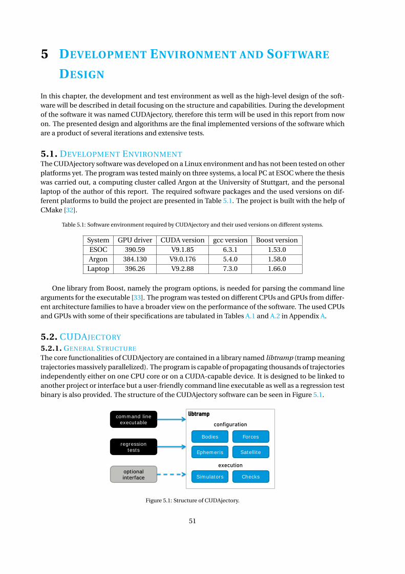
5 DEVELOPMENT ENVIRONMENT AND SOFTWARE
DESIGN
In this chapter, the development and test environment as well as the high-level design of the soft-ware will be described in detail focusing on the structure and capabilities. During the developmentof the software it was named CUDAjectory, therefore this term will be used in this report from nowon. The presented design and algorithms are the final implemented versions of the software whichare a product of several iterations and extensive tests.
5.1. DEVELOPMENT ENVIRONMENTThe CUDAjectory software was developed on a Linux environment and has not been tested on otherplatforms yet. The program was tested mainly on three systems, a local PC at ESOC where the thesiswas carried out, a computing cluster called Argon at the University of Stuttgart, and the personallaptop of the author of this report. The required software packages and the used versions on dif-ferent platforms to build the project are presented in Table 5.1. The project is built with the help ofCMake [32].
Table 5.1: Software environment required by CUDAjectory and their used versions on different systems.
System GPU driver CUDA version gcc version Boost versionESOC 390.59 V9.1.85 6.3.1 1.53.0Argon 384.130 V9.0.176 5.4.0 1.58.0
Laptop 396.26 V9.2.88 7.3.0 1.66.0
One library from Boost, namely the program options, is needed for parsing the command linearguments for the executable [33]. The program was tested on different CPUs and GPUs from differ-ent architecture families to have a broader view on the performance of the software. The used CPUsand GPUs with some of their specifications are tabulated in Tables A.1 and A.2 in Appendix A.
5.2. CUDAJECTORY
5.2.1. GENERAL STRUCTURE
The core functionalities of CUDAjectory are contained in a library named libtramp (tramp meaningtrajectories massively parallelized). The program is capable of propagating thousands of trajectoriesindependently either on one CPU core or on a CUDA-capable device. It is designed to be linked toanother project or interface but a user-friendly command line executable as well as a regression testbinary is also provided. The structure of the CUDAjectory software can be seen in Figure 5.1.
libtramp
configuration
execution
Bodies Forces
ChecksSimulators
Ephemeris
command line executable
regressiontests
optionalinterface
Satellite
Figure 5.1: Structure of CUDAjectory.
51

52 5. DEVELOPMENT ENVIRONMENT AND SOFTWARE DESIGN
There are several configuration modes of the project which use different compiler options. Thesoftware can be built in release, debug, and profile modes. The profile mode only differs from therelease mode in nvcc’s --generate-line-info flag which generates line number information onlyfor device code, that can be used later for profiling [34]. Additionally, the user can configure CU-DAjectory using only single-precision floating-point format with the option to enable CUDA’s fastmath library. The fast math library contains optimized instructions for arithmetic operations andthe evaluations of transcendental functions, such as sine and cosine, but at a cost of less accuracy.However it will be shown that single-precision calculation is simply not accurate enough for trajec-tory propagation. There is an option to compile and build the code in verbose mode, which printsadditional information such as register, global and constant memory usage of functions as well asregister spillage data. This information is crucial for code optimization as mentioned in Section2.6.8.
5.2.2. CAPABILITIES
A more detailed description of the capabilities and the configurable settings of libtramp can be seenin Figure 5.2.
Bodies Forces ChecksSimulatorsEphemeris
Physical bodies
Barycenters
Third-body perturbation
Spherical harmonics
J2
Point mascon model
Solar radiation pressure
RKF78
Clustered RKF78
JPL ephemerides Collision
Altitude
SOI crossing
• Bodycentric form• Barycentric form
Pauses simulation to• sort samples• collect output
Optionally switches the centre of propagation
Aborts samples
Satellite
Area to mass ratio
Reflectivity coefficient
Dual cone shadow model
Figure 5.2: Capabilities and configurable settings of CUDAjectory (libtramp).
The user can provide the initial states of the samples in a Comma-Separated Values (CSV) fileusing MJD2000 and TDB as time representation and system and Cartesian coordinates with unitsof km and km/s for the position and velocity. The center of propagation has to be set consistentlywith the input data. In the current version of CUDAjectory the time period of the simulation is thesame for each sample which can be set in days. However, if a certain application requires differ-ent simulation periods for the samples, the program can be easily modified to be able to set thesevarious periods, but it would require some additional memory which could theoretically lead toperformance loss.
The dynamical model can be set by applying different force models, which were discussed inSection 3.2, in the configuration. If the center of propagation is the Solar System barycenter thenEq. (3.9) is used to describe the motion of the satellite using the planets, Pluto, Moon and Sun ascontributing bodies. If the center of propagation is a physical body then Eq. (3.12) is used, where thefirst (two-body) term of the equation is mandatory regardless of the user provided model settings.The evaluation of the planetary ephemerides is done by using the JPL ephemeris model describedin Section 3.3. The satellite properties (reflectivity coefficient and area-to-mass ratio) are necessaryfor the SRP calculation. The dual-cone shadow model can optionally be used to calculate eclipse

5.2. CUDAJECTORY 53
conditions with multiple occulting bodies which are described in Section 3.2.3.
As mentioned before, the used integrator in CUDAjectory is the RKF78 which can be used infixed and adaptive time step mode. The user can configure the initial step size, the absolute andrelative tolerance of the integration as well as the minimum and maximum step sizes. Additionally,the maximum number of attempts to recalculate a step can also be set by the user.
There is a possibility for clustering the input samples during the simulation. It will be shownin Section 7.3 that this method can significantly reduce the execution time in certain cases runningon a GPU. If clustering is enabled the simulation pauses after a user defined number of integrationsteps (regardless the fact that the step was successful or not), samples are sorted by current epochand output is optionally collected if there was any and then the simulation continues. It is possibleto optionally save the state of every sample in a CSV file if clustering is enabled, however this wouldsignificantly increase the execution time, since it requires a large number of I/O operations.
Checks can be optionally performed during the simulation, some of which produce secondarydata. The collision check detects if the satellite penetrated a body’s surface and aborts its propaga-tion after impact. The user can set an altitude offset to each body to detect "collisions" at a certainaltitude above the surface of the bodies. Note that the exact time of the collision is not determinedwhich could have been done using some mathematical method such as the bisection method, how-ever it would significantly increase the execution time. Therefore, only the first occasion when thedistance between the body and the satellite is less than its radius is recorded. During an altitudecheck the satellite’s altitude with respect to the central body can be saved in a CSV file. The SphereOf Influence (SOI) crossing check detects if the satellite had crossed the sphere of influence of abody. It is possible that after a SOI crossing the center of propagation is changed to the body, whoseSOI the satellite has entered.
The user can define warning messages and raise them during the simulation, which do not ter-minate the execution. The messages that have been implemented relate to the variable step size in-tegration such as exceeding the limit for a minimum or maximum step size or number of attemptsto calculate a successful step. It is also possible to define error messages and raise errors whichterminate the execution.
5.2.3. GENERAL ALGORITHMIC MODEL
SIMULATION
CUDAjectory has two execution modes when it comes to hardware: the CPU and GPU modes. TheCPU mode propagates the trajectories sequentially and does not involve any parallelism. The GPUmode propagates the trajectories in parallel using one GPU device. Some part of the total simulationin GPU mode is also executed on the CPU as it was introduced in the heterogeneous programmingmodel in Section 2.6.3, however, the propagation is completely executed on the GPU. The generalhigh-level algorithmic model of CUDAjectory can be seen in Figure 5.3.
After the CUDAjectory executable starts, the program reads the configuration from the com-mand line and a configuration file. The software then reads the input CSV file which contains theinitial states and initializes the integrator, force models, ephemeris data, etc. Note that in case of amodel requiring additional data such as ephemeris or spherical harmonics coefficients, the user hasto provide that in a file in a given format, which will be processed during initialization. If GPU modeis set, then all the model data is copied to the device and placed in different memory regions suchas global memory, constant memory, or texture memory. The utilization of different GPU mem-ory regions will be discussed in detail in Chapter 7. If CPU mode is selected, the propagation startsimmediately after initialization since all the required data is already in CPU memory. After the prop-agation is finished, the final states are written in a CSV file. The allocated memory on the CPU andthe GPU is freed and the software finishes execution.

54 5. DEVELOPMENT ENVIRONMENT AND SOFTWARE DESIGN
Copy data to GPU
Read configuration and initial states
Start
Exit
Initialize integrator, force
models, ephemerisSimulator Write final states
to CSV fileFree
memory
CPU: GPU: CPU/GPU:
Figure 5.3: General high level algorithmic model of CUDAjectory.
PROPAGATION
There are two propagation algorithms in CUDAjectory, which are shown under the Simulators boxin Figure 5.2. The RKF78 simulator simply takes the input samples in the same order as they werein the input file and, in CPU mode, propagates them sequentially, in GPU mode, propagates themin parallel. In GPU mode, one thread represents one sample, therefore the number of launchedthreads is equal to the number of samples. Note that simulating high number of samples is not apractical issue, because the theoretical maximum number of threads that can be launched reachestrillions on devices with at least Compute Capability 3.0 [18]. It will be shown in Chapter 8 that highnumber of samples, approximately 10000-100000 depending on the device that is used, is desiredto achieve the best performance.
Since the number of integration steps is not known in advance for a variable step size integra-tion, there is no possibility to collect data during the simulation, only the final states can be seen bythe user. The general algorithmic model of the clustered RKF78 simulator in GPU mode can be seenin Figure 5.4.
Sortsamples
Copy samples to
GPU
Propagate N samples for
m steps
Copy samples to
CPU
Write output to CSV files
Unfinished samples
noyes
: main thread : second thread
Filter samples
Figure 5.4: Algorithmic model of the clustered RKF78 simulator.
This simulator breaks the propagation and returns to the host after a configurable number ofintegration step attempts, denoted m in the figure, to sort and filter the samples or collect output.
5.2. CUDAJECTORY 55
The term attempt has to be emphasized here, because during variable time step integration it is notnecessarily true that the calculation of the next integration step is within the configured error limit,therefore a new step has to be calculated with a different step size, which counts as an additionalintegration step attempt. The number of integration step attempts m will be called break size forsimplicity from now on. Since the break size is a user defined parameter, setting it to an optimalvalue is extremely important. The effect of choosing different break sizes will be discussed in detailin Section 7.3. It will be shown that as a rule of thumb, values between 200 and 400 can be an optimalchoice for most of the applications.
Sorting is simply done by the current epochs of the samples, however sorting and clusteringby other attributes or multiple attributes can be easily implemented as well. The current epochwas chosen as an attribute for sorting because it leads to more efficient caching if ephemeris datais used as will be discussed in Section 7.3. It can be seen in the figure that collecting and writingthe output to CSV files can be done asynchronously with the sorting, filtering and propagation ofthe next batch which significantly reduces the execution time. If the propagation of the next batch isfinished before the writing of the output, then the main thread halts until the second thread finishesits job. Asynchronous output handling will be discussed in more detail in Section 7.4. Filtering isdone by selecting the samples that have already finished propagation or have impacted a body, sincethere is no need to further copy their data to the GPU. This method can reduce the number of idlingthreads, which can lead to a significant performance gain. If all samples are finished, the executioncontinues with the next step in the algorithm.


6 VERIFICATION AND VALIDATION
Verification and validation of every new implementation of a problem is a crucial part in its assess-ment. Unfortunately, analytical solutions are not available for most of the models that have beenpresented in Section 3.2, therefore the results of CUDAjectory will be compared to a validated soft-ware called MASW (Mission Analysis Software) that was developed at the Mission Analysis Sectionat ESOC. There are several software available at the Mission Analysis Section which have been usedfor past missions and will be used for future missions as well. Each software is specialized for acertain purpose to maximize their performance. MASW is written in C++ and it is the most robusttoolbox available, therefore it was chosen to validate CUDAjectory.
A random orbit and epoch was selected for validation of each module of CUDAjectory. The two-body problem will be validated by comparing to the analytical solution, and every other model willbe compared to MASW. The selected orbit is the following with Earth as a central body:
a = 7000 km
e = 0.05
i = 45 deg
Ω= 30 deg
ω= 30 deg
θ = 50 deg
(6.1)
The simulation start epoch t0 was selected differently according to the configuration of the software,because in single-precision mode it is possible that the time steps are small enough that two consec-utive epochs are numerically the same in the MJD2000 time representation since single-precisionallows only approximately 9 digits of precision. If the epochs in MJD2000 are small enough thisproblem is not present in single-precision mode. The simulation duration was selected to be fivedays during which the spacecraft makes roughly 75 orbital revolutions.
6.1. TWO-BODY PROBLEMThe analytical solution of the two-body problem is well known therefore it is a good case to validatethe implemented integrator. According to the solution of the two-body problem, the orbital ele-ments do not change over time except the true anomaly which can be calculated by solving Kepler’sequation [21]:
M = E −e sinE (6.2)
where M is the mean anomaly, e is the eccentricity, and E is the eccentric anomaly. The relationbetween the eccentric anomaly and the true anomaly is the following [21]:
tanθ
2=
√1+e
1−etan
E
2(6.3)
The mean anomaly can be calculated from the reference time of the integration as follows [21]:
M = M0 +n(t − t0) (6.4)
57

58 6. VERIFICATION AND VALIDATION
where M0 is the mean anomaly at time t0, n is the mean angular motion, t is the current epoch, andt0 is the start epoch.
The comparison of the analytical solution with the integration in single-precision and double-precision modes using a CPU can be seen in Figure 6.1.
Figure 6.1: Difference between the analytical solution of the two-body problem and the integration using single- (top)and double-precision (bottom) with 10−9 integration tolerance on a CPU.
The integration tolerance was chosen to be 10−9 because that is generally the limit for single-precision calculations. This tolerance gave approximately 50 seconds as an average time step forsingle- and 200 seconds for double-precision calculations. It can be seen that the difference be-
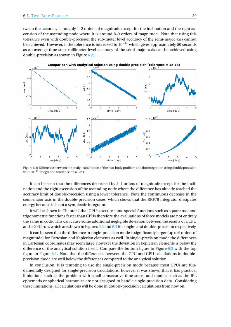
6.1. TWO-BODY PROBLEM 59
tween the accuracy is roughly 1–2 orders of magnitude except for the inclination and the right as-cension of the ascending node where it is around 8–9 orders of magnitude. Note that using thistolerance even with double-precision the sub-meter level accuracy of the semi-major axis cannotbe achieved. However, if the tolerance is increased to 10−14 which gives approximately 50 secondsas an average time step, millimeter level accuracy of the semi-major axis can be achieved usingdouble-precision as shown in Figure 6.2.
Figure 6.2: Difference between the analytical solution of the two-body problem and the integration using double precisionwith 10−14 integration tolerance on a CPU.
It can be seen that the differences decreased by 2–4 orders of magnitude except for the incli-nation and the right ascension of the ascending node where the difference has already reached theaccuracy limit of double-precision using a lower tolerance. Note the continuous decrease in thesemi-major axis in the double-precision cases, which shows that the RKF78 integrator dissipatesenergy because it is not a symplectic integrator.
It will be shown in Chapter 7 that GPUs execute some special functions such as square root andtrigonometric functions faster than CPUs therefore the evaluations of force models are not entirelythe same in code. This can cause some additional negligible deviation between the results of a CPUand a GPU run, which are shown in Figures 6.3 and 6.4 for single- and double-precision respectively.
It can be seen that the difference in single-precision mode is significantly larger (up to 9 orders ofmagnitude) for Cartesian and Keplerian elements as well. In single-precision mode the differencesin Cartesian coordinates may seem large, however the deviation in Keplerian elements is below thedifference of the analytical solution itself. Compare the bottom figure in Figure 6.3 with the topfigure in Figure 6.1. Note that the differences between the CPU and GPU calculations in double-precision mode are well below the differences compared to the analytical solution.
In conclusion, it is tempting to use the single-precision mode because most GPUs are fun-damentally designed for single-precision calculations, however it was shown that it has practicallimitations such as the problem with small consecutive time steps, and models such as the JPLephemeris or spherical harmonics are not designed to handle single-precision data. Consideringthese limitations, all calculations will be done in double-precision calculations from now on.

60 6. VERIFICATION AND VALIDATION
Figure 6.3: Difference between CPU and GPU Cartesian (top) and Keplerian (bottom) results using single-precision.
6.2. THIRD-BODY PERTURBATION
The following force models including the third-body perturbations will be validated using the MASWsoftware as a reference. It is not possible to use fixed time step integration of the RKF78 in MASW,therefore Verner’s Runge–Kutta 8(7) integrator was selected for validation [35]. This integrator usesthe so-called dense interpolation scheme to determine the state at any time between two integra-tion steps with the accuracy of the lower solution of the embedded pair, which is in this case 7thorder. The simulation start epoch t0 was set to be 6000 MJD2000 which is 5th of June 2016 in calen-dar date. Both software use the same ephemeris data and integration tolerance.

6.2. THIRD-BODY PERTURBATION 61
Figure 6.4: Difference between CPU and GPU Cartesian (top) and Keplerian (bottom) results using double-precision.
The differences between MASW and the CPU version of CUDAjectory are shown in Figure 6.5. Itcan be seen in the figure that the differences are at the centimeter level for the position coordinatesand extremely noisy, which shows it is coming from numerical inaccuracies. The magnitude of thedifferences is probably the accuracy limit of the interpolation.
The difference between the CPU and GPU version of CUDAjectory can be seen in Figure 6.6.Fixed time step integration using 50 seconds step size was used in this comparison to avoid addi-tional interpolation errors. The differences in the position coordinates are sub-millimeter in mag-nitude and they show an increasing pattern in time. It can be concluded that due to the small mag-

62 6. VERIFICATION AND VALIDATION
Figure 6.5: Difference between CUDAjectory and MASW using the Sun and the Moon as perturbing bodies.
nitude of the deviation between the CPU and GPU versions compared to the difference betweenthe CPU version and MASW, the comparison between the GPU version and MASW is not necessary.Considering the results it can be concluded that the third-body perturbation model is validated.
Figure 6.6: Difference between the CPU and GPU version of CUDAjectory using the Sun and the Moon as perturbingbodies with fixed time step integration.

6.3. J2 EFFECT 63
6.3. J2 EFFECT
The difference between MASW and the CPU version of CUDAjectory considering the J2 effect ofEarth can be seen in Figure 6.7. It can be seen that the pattern and magnitude is similar to the third-body perturbation and it is probably caused by the interpolation again. The frame transformationbetween Earth fixed and inertial is done using the same method in both software.
Figure 6.7: Difference between CUDAjectory and MASW using J2 perturbation.
The difference between the CPU and GPU versions of CUDAjectory using J2 as a perturbingeffect can be seen in Figure 6.8.
Figure 6.8: Difference between the CPU and GPU version of CUDAjectory using J2 perturbation with fixed time stepintegration.

64 6. VERIFICATION AND VALIDATION
It will be explained in Chapter 7 that during the frame transformation, there is a difference inthe implementation of the two modes, which could cause additional discrepancy in the results.However, it can be seen that even with this additional source of error the difference is still at thesub-millimeter level and therefore negligible. It can be concluded that the J2 model is validated.
6.4. SPHERICAL HARMONICSThe coefficients of the spherical harmonics model were taken from the EIGEN-05C model, whereEIGEN stands for European Improved Gravity model of the Earth by New techniques [36]. Themodel was developed by GFZ Potsdam, and it is a combination of GRACE and LAGEOS missionmeasurements plus gravimetry and altrimetry surface data. The difference between MASW and theCPU version of CUDAjectory considering the spherical harmonics model of Earth with degree andorder 10 can be seen in Figure 6.9.
Figure 6.9: Difference between CUDAjectory and MASW using spherical harmonics up to degree and order 10.
It can be seen in the figure that the magnitude (centimeter level for position coordinates) of thedifferences is again the same as in the third-body perturbation and the J2 case and it is probablycaused by the dense interpolation. Note that CUDAjectory uses normalized gravitational coeffi-cients whereas MASW uses unnormalized coefficients, which could be a source of numerical error.The difference between the CPU and GPU results of CUDAjectory can be seen in Figure 6.10.
Similarly to the J2 case, an additional source of inequality is the different implementation of theframe transformation which is required to calculate the accelerations caused by the spherical har-monics model. The difference between the two versions is well below sub-millimeter level thereforenegligible. Note that there is some periodic pattern in the differences which are probably caused bythe changes in the orbital elements induced by the irregular gravity field. Considering the results,the spherical harmonics model and the frame transformation algorithm are validated.
6.5. POINT MASCON MODELThere is no implementation of the point mascon model in MASW, therefore it will be compared tothe spherical harmonics model implemented in CUDAjectory. The point mascon model created

6.6. SOLAR RADIATION PRESSURE 65
Figure 6.10: Difference between the CPU and GPU version of CUDAjectory using spherical harmonics up to degree andorder 10 with fixed time step integration.
in [26] uses the truncated spherical harmonics evaluations from the GGM02C gravity field derivedfrom the GRACE mission, thus this gravity model will be used in the spherical harmonics compar-ison. As described in Section 3.2 the number of mascons increases with the higher-fidelity gravitymodel, and the positions and gravitational parameters of each mascon were derived using the leastsquares method. The difference between the spherical harmonics model using degree and order 27and the corresponding point mascon model equivalent, which has 960 mascons, running the CPUversion of CUDAjectory can be seen in Figure 6.11.
The comparison was repeated using all available point mascon models with different numberof mascons which correspond to different fidelity in the spherical harmonics model. The magni-tude of the differences varied between millimeter and meter level, however there was no correlationbetween the fidelity and the differences. In this particular example (degree and order 27) the dif-ferences in the position coordinates are showing a non-symmetrical pattern and have a magnitudebelow one meter. The difference between the CPU and GPU results can be seen in Figure 6.12.
It can be seen that the differences are two orders of magnitude higher than in the previous mod-els, however they are still at millimeter level for the position coordinates. This increased differenceis due to the large number of point mass gravity acceleration additions, which is in this particularcase was 960. Small deviations in the individual acceleration evaluations simply accumulate whichcauses larger differences. Considering all the results, the point mascon model is validated.
6.6. SOLAR RADIATION PRESSUREThe shadow factor in Eq. (3.33) can be determined by the dual-cone shadow model which is used inMASW as well. However, CUDAjectory can be configured such that it does not determine the eclipseconditions to save computation time and assumes that the satellite is in constant sunlight which isusually true for interplanetary trajectories. During the comparison, the reflectivity coefficient Cr
was chosen to be 1.2, and the area to mass ratio Ar /m was chosen to be 0.1 m2/kg. The differencebetween CUDAjectory and MASW using SRP can be seen in Figure 6.13.

66 6. VERIFICATION AND VALIDATION
Figure 6.11: Difference between the spherical harmonics model up to degree and order 27 and the point mascon modelusing CPU version of CUDAjectory with fixed time step integration.
Figure 6.12: Difference between the CPU and GPU version of CUDAjectory using point mascon model with 960 mascons(spherical harmonics with degree and order 27 equivalent) with fixed time step integration.
It can be seen in the figure that the difference has increased by an order of magnitude comparedto the previous cases, which is probably caused by the heavy usage of special functions such asthe inverse trigonometric functions, which can lead to higher numerical inaccuracies. Additionally,extra parameters such as the radii of the Sun and Earth have to be used to calculate the eclipse con-ditions, thus small deviations in these parameters can also cause differences between the results.The difference between the CPU and GPU results using SRP can be seen in Figure 6.14.

6.7. COMBINED TEST CASE 67
Figure 6.13: Difference between CUDAjectory and MASW using SRP.
Figure 6.14: Difference between the CPU and GPU version of CUDAjectory using SRP with fixed time step integration.
There is no recommendation in [37] how to effectively utilize inverse trigonometrical functionson a GPU, therefore the same code is used to calculate the eclipse conditions in both modes. How-ever, there are instruction-level differences in the calculation of the acceleration similarly to theprevious models. The differences are well below sub-millimeter level therefore negligible. Consid-ering the results of these tests, the SRP perturbation and the eclipse detection model is validated.
6.7. COMBINED TEST CASETo test all models acting together, an additional case was created which uses the Sun and Moon asperturbing bodies, spherical harmonics up to degree and order 10, and SRP. The differences be-tween CUDAjectory and MASW can be seen in Figure 6.15.
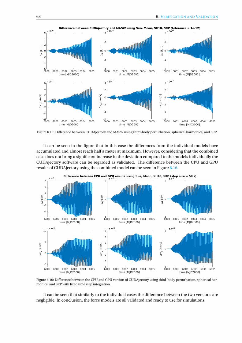
68 6. VERIFICATION AND VALIDATION
Figure 6.15: Difference between CUDAjectory and MASW using third-body perturbation, spherical harmonics, and SRP.
It can be seen in the figure that in this case the differences from the individual models haveaccumulated and almost reach half a meter at maximum. However, considering that the combinedcase does not bring a significant increase in the deviation compared to the models individually theCUDAjectory software can be regarded as validated. The difference between the CPU and GPUresults of CUDAjectory using the combined model can be seen in Figure 6.16.
Figure 6.16: Difference between the CPU and GPU version of CUDAjectory using third-body perturbation, spherical har-monics, and SRP with fixed time step integration.
It can be seen that similarly to the individual cases the difference between the two versions arenegligible. In conclusion, the force models are all validated and ready to use for simulations.

7 SOFTWARE OPTIMIZATION
This chapter will describe the main algorithmic and design aspects of the software which led tosignificant performance increase. Optimization at different levels will be discussed from instruc-tion level to efficient memory usage. The various optimization techniques mainly affect the perfor-mance of the GPU execution.
7.1. INSTRUCTION OPTIMIZATIONLow-level optimization, such as instruction optimization, is essentially favorable in code that is runfrequently and has a simple structure. NVIDIA provided a guide to their devices which suggestssome optimization aspects to developers at an instruction level, which can be found in Chapter 11of the CUDA C Best Practices Guide [37].
It is recommended to use the reciprocal square root function rsqrt() instead of 1.0/sqrt() wherepossible. It can be seen in most of the equations of the force models in Section 3.2 that they containthe norm of a vector to the power of minus three. The implementation of these expressions canbe done by utilizing the reciprocal square root function. Note that this function is not available forCPUs, therefore in the CPU version the sqrt() function is used. Since the precision of these twofunctions is different, this optimization will inherently lead to a small inequality in the results of theCPU and GPU versions of the software. A 1-2% performance increase can be achieved after applyingthis optimization for evaluating the two-body, third-body, J2, etc. models.
It can be seen in Section 3.1.3 that during a frame transformation numerous sin() and cos()function evaluations are needed. CUDA provides the function sincos(), which is not available instandard C++, that calculates the sine and cosine of an angle using only one function. There isanother version of this function namely sincospi(<expr>) which is equivalent of sincos(π*<expr>).This version is advantageous with regards to both accuracy and performance. Since the data takenfrom [25] is given in degrees, the implemented frame transformation algorithm also requires therotational angles to be given in degrees, therefore the sincospi(<expr>/180.0) function can be usedto obtain the sine and cosine of these angles [37]. An additional 1-2% performance increase can begained by applying this optimization during evaluating of the frame transformations.
7.2. KERNEL PROFILINGSeveral tools were mentioned in Section 2.6.8 which can help the developer to debug, profile andoptimize the software. One of the most convenient of these is the NVIDIA Profiling Tools, which isable to detect bottlenecks in the code and provide metrics of the software’s performance. Addition-ally, the CUDA Occupancy Calculator can help to detect which resource, such as shared memory orregister usage, limits the GPU to achieve higher occupancy without running the program.
7.2.1. OCCUPANCY
After building the program with nvcc’s --ptxas-options=-v compiler flag the registers per threadand shared memory per block resource usage of a kernel can be obtained. Since there is no inter-action between any thread, shared memory would serve as a global memory storage, and for thatpurpose constant memory is already utilized, therefore shared memory will not be used in CUDA-jectory. Consequently the only limiter for occupancy is the register usage of the threads. The num-ber of registers used per thread can be different building for different GPUs. For Compute Capability3.0 the number of registers used is 63, and for newer Compute Capabilities it is 128. Note that themaximum number of registers is 63 for Compute Capability 3.0 and 255 since Compute Capability3.2 [18]. The impact of varying register usage using 128 threads-per-block for Compute Capability3.0 and Compute Capability 5.0, 6.0 and 6.1 can be seen in Figure 7.1.
69

70 7. SOFTWARE OPTIMIZATION
Figure 7.1: Impact of varying register count per thread using Compute Capability 3.0 (top) and Compute Capability 5.0,6.0, 6.1 (bottom).
It can be seen that the number of registers has to be reduced significantly before achieving anyincrease in the occupancy, which is theoretically limited to 50% for Compute Capability 3.0, and25% for Compute Capability 5.0 and newer. Note that in this particular case the occupancy us-ing Compute Capability 3.0 or newer are overlapping between the 0 and 63 register interval whichis not the case for arbitrary settings. The compiler can be forced to use less registers with nvcc’s--maxrregcount flag during code generation, which can increase the occupancy. However, forcingthe compiler to use less registers can lead to register spilling which causes decreased performance.Register spilling happens if some variables in a function cannot be fit into the registers, thereforethey spilled to local memory that resides in the DRAM of the GPU, which has significantly lowerbandwidth than the registers. Since the number of registers has to be limited significantly to achievehigher occupancy, register spilling becomes an issue. This phenomenon was tested thoroughly andindeed limiting the number of registers caused performance decrease. The impact of varying thenumber of threads in a block for different Compute Capabilities can be seen in Figure 7.2.
It can be seen that there are several values for the block size which theoretically allow the sameoccupancy. 50% theoretical maximum occupancy can be achieved by using 64, 128, 256, 512, or 1024threads-per-block with Compute Capability 3.0. Compiling with Compute Capability 5.0 or higheronly 25% maximum occupancy can be achieved by using 32, 64, 128, 256, or 512 threads-per-block.After some testing using different configurations 128 was chosen to be a good value for most of thecases. Note that the occupancy goes down to zero if the threads-per-block value is above 512, whichmeans that the program will produce a runtime error since the kernel cannot be launched with thisconfiguration.
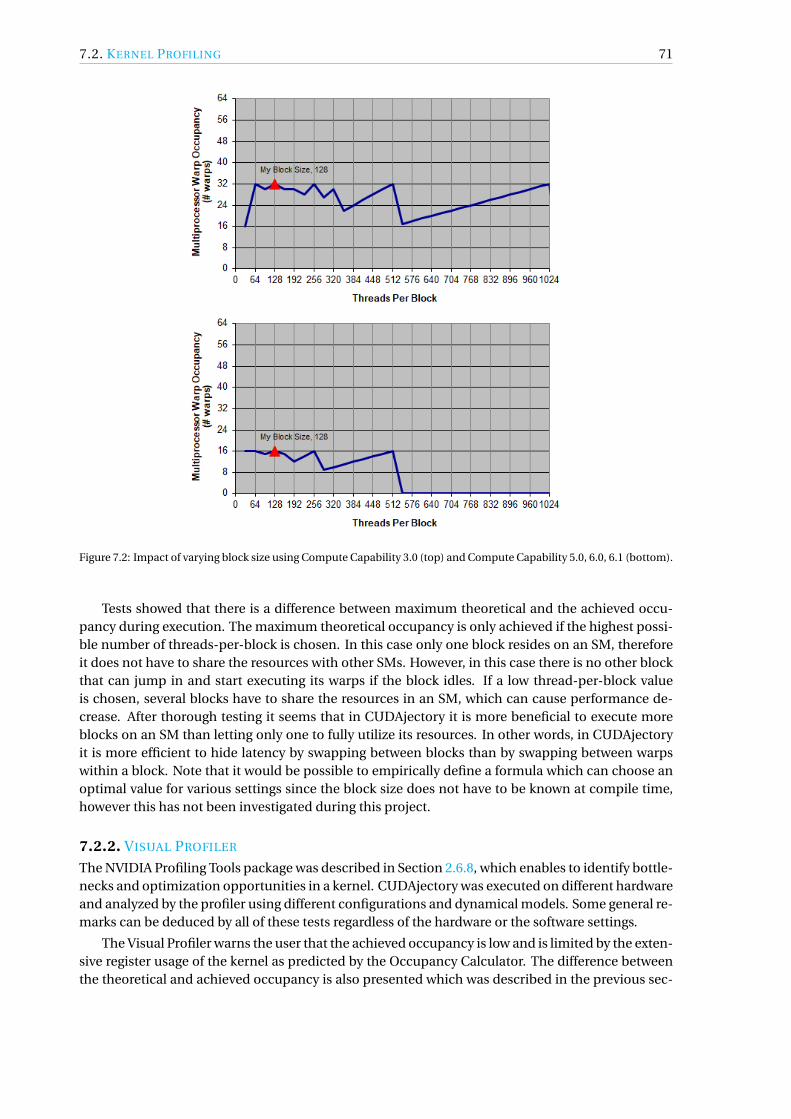
7.2. KERNEL PROFILING 71
Figure 7.2: Impact of varying block size using Compute Capability 3.0 (top) and Compute Capability 5.0, 6.0, 6.1 (bottom).
Tests showed that there is a difference between maximum theoretical and the achieved occu-pancy during execution. The maximum theoretical occupancy is only achieved if the highest possi-ble number of threads-per-block is chosen. In this case only one block resides on an SM, thereforeit does not have to share the resources with other SMs. However, in this case there is no other blockthat can jump in and start executing its warps if the block idles. If a low thread-per-block valueis chosen, several blocks have to share the resources in an SM, which can cause performance de-crease. After thorough testing it seems that in CUDAjectory it is more beneficial to execute moreblocks on an SM than letting only one to fully utilize its resources. In other words, in CUDAjectoryit is more efficient to hide latency by swapping between blocks than by swapping between warpswithin a block. Note that it would be possible to empirically define a formula which can choose anoptimal value for various settings since the block size does not have to be known at compile time,however this has not been investigated during this project.
7.2.2. VISUAL PROFILER
The NVIDIA Profiling Tools package was described in Section 2.6.8, which enables to identify bottle-necks and optimization opportunities in a kernel. CUDAjectory was executed on different hardwareand analyzed by the profiler using different configurations and dynamical models. Some general re-marks can be deduced by all of these tests regardless of the hardware or the software settings.
The Visual Profiler warns the user that the achieved occupancy is low and is limited by the exten-sive register usage of the kernel as predicted by the Occupancy Calculator. The difference betweenthe theoretical and achieved occupancy is also presented which was described in the previous sec-

72 7. SOFTWARE OPTIMIZATION
tion. The profiler shows the reasons for an instruction stall in a pie chart which can be seen inFigure 7.3. Unfortunately the profiler is not capable of showing the quantity of the stall, only theratio between the reasons that is causing it.
Figure 7.3: Instruction stall reasons for Quadro GP100 (left) and GeForce GTX 1080 Ti (right) produced by the NVIDIAVisual Profiler.
It can be seen that the main reason for an instruction stall is memory dependency for both GPUs,which occurs when a load or store instruction cannot be made because the required resources arenot available. The second largest reason depends on the GPU family. For computing accelerators,such as the Quadro GP100, which have much higher throughput than gaming cards, the secondlargest stall reason is instruction fetch, which occurs if the next assembly instruction has not beenfetched. For gaming cards, such as the GeForce GTX 1080 Ti, it is execution dependency whichoccurs if an input required by an instruction is not yet available. The figure shows that these threereasons are causing most of the stalls during the simulation, which was expected since the softwarerequires a large number of memory load instructions for loading data for the different models.
The profiler can also show the utilization level of the resources in an SM such as the specialfunction units or load and store units. The execution unit utilization can be seen in Figure 7.4.
Figure 7.4: Execution unit utilization for Quadro GP100 (top) and GeForce GTX 1080 Ti (bottom) produced by the NVIDIAVisual Profiler.
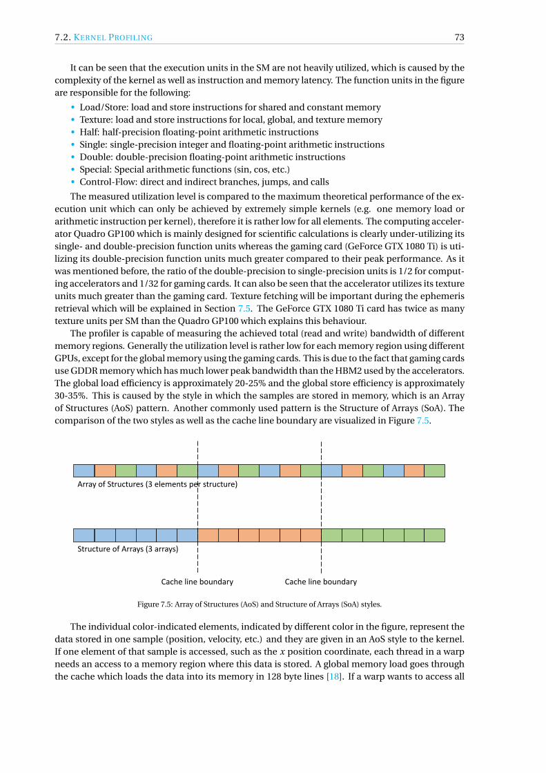
7.2. KERNEL PROFILING 73
It can be seen that the execution units in the SM are not heavily utilized, which is caused by thecomplexity of the kernel as well as instruction and memory latency. The function units in the figureare responsible for the following:
• Load/Store: load and store instructions for shared and constant memory• Texture: load and store instructions for local, global, and texture memory• Half: half-precision floating-point arithmetic instructions• Single: single-precision integer and floating-point arithmetic instructions• Double: double-precision floating-point arithmetic instructions• Special: Special arithmetic functions (sin, cos, etc.)• Control-Flow: direct and indirect branches, jumps, and calls
The measured utilization level is compared to the maximum theoretical performance of the ex-ecution unit which can only be achieved by extremely simple kernels (e.g. one memory load orarithmetic instruction per kernel), therefore it is rather low for all elements. The computing acceler-ator Quadro GP100 which is mainly designed for scientific calculations is clearly under-utilizing itssingle- and double-precision function units whereas the gaming card (GeForce GTX 1080 Ti) is uti-lizing its double-precision function units much greater compared to their peak performance. As itwas mentioned before, the ratio of the double-precision to single-precision units is 1/2 for comput-ing accelerators and 1/32 for gaming cards. It can also be seen that the accelerator utilizes its textureunits much greater than the gaming card. Texture fetching will be important during the ephemerisretrieval which will be explained in Section 7.5. The GeForce GTX 1080 Ti card has twice as manytexture units per SM than the Quadro GP100 which explains this behaviour.
The profiler is capable of measuring the achieved total (read and write) bandwidth of differentmemory regions. Generally the utilization level is rather low for each memory region using differentGPUs, except for the global memory using the gaming cards. This is due to the fact that gaming cardsuse GDDR memory which has much lower peak bandwidth than the HBM2 used by the accelerators.The global load efficiency is approximately 20-25% and the global store efficiency is approximately30-35%. This is caused by the style in which the samples are stored in memory, which is an Arrayof Structures (AoS) pattern. Another commonly used pattern is the Structure of Arrays (SoA). Thecomparison of the two styles as well as the cache line boundary are visualized in Figure 7.5.
Array of Structures (3 elements per structure)
Structure of Arrays (3 arrays)
Cache line boundary Cache line boundary
Figure 7.5: Array of Structures (AoS) and Structure of Arrays (SoA) styles.
The individual color-indicated elements, indicated by different color in the figure, represent thedata stored in one sample (position, velocity, etc.) and they are given in an AoS style to the kernel.If one element of that sample is accessed, such as the x position coordinate, each thread in a warpneeds an access to a memory region where this data is stored. A global memory load goes throughthe cache which loads the data into its memory in 128 byte lines [18]. If a warp wants to access all

74 7. SOFTWARE OPTIMIZATION
the blue elements using the AoS pattern it needs three cache line request, whereas using the SoApattern it only needs one request. Because the code has numerous sample data accesses, it wouldbe more efficient for memory coalescence if the samples were stored in a SoA style, however it wouldmake the expandability and readability of the code much worse. The SoA style is a more natural wayof storing the sample data in an object-oriented language such as C++ and it is much easier to passsome parts such as the position of a sample as an argument to a function, therefore it was chosen asa final implementation regardless of the possibly worse performance.
The profiler also raises a warning that local memory overhead is high, which indicates excessiveregister spilling, although the register usage of the kernel is already high. Further increasing the reg-ister count would probably decrease the local memory overhead, however the achieved occupancywould be even lower, which would decrease performance.
Warp divergence can also be detected by the profiler, which can occur in several places. Thanksto nvcc’s --generate-line-info flag, the profiler is able to tell the user the exact file name andline number where the divergence occurs. In CUDAjectory, as expected, threads diverge in the in-tegrator’s code segment when the logic is executed which evaluates if the step was within the giventolerance. It is possible that not all threads within the same warp had a valid or an invalid stepwhich leads to warp divergence. However, this logic is a necessary step during variable step size in-tegration, therefore divergence is inevitable. The other occasion of warp divergence appears duringsphere of influence crossings. If some threads within the same warp are in different body’s sphere ofinfluence, the execution of some code segments might be different. This divergent execution can bealleviated by frequent clustering by the position of the samples, therefore there is a higher chancethat samples that are in the same sphere of influence of a body will be in the same warp. Note thatin most cases, the divergence caused by this problem is much less than caused by the integrator.
7.3. SAMPLE CLUSTERINGThe algorithmic model of the clustered RKF78 simulator was already presented in Section 5.2.3. Asmentioned, clustering of the samples is done by the current epochs during the sorting phase. A testwas conducted to demonstrate the effect of clustering on the runtimes using different break sizes.The break size is the number of integration steps after the control returns to the host to filter andsort the samples and collect the output. A series of random heliocentric trajectories was generatedwith the following initial epoch and Keplerian elements:
t0 ∈ [−14000 MJD2000,16000 MJD2000]
a ∈ [1.1 AU,1.2 AU]
e ∈ [0,0.02]
i ∈ [0,9]
Ω ∈ [0,360]
ω ∈ [0,360]
θ ∈ [0,360]
(7.1)
Note that the inclination of the samples was deliberately reduced to get a planet-like trajectory. Thedynamical model used in this test was to include all Solar System planets, Pluto and the Moon asperturbing bodies. Any orbit chosen from this set results in similar behaviour, because there are noflybys or close approaches with any planet. The number of samples in these simulations was fixedto 10000 and the propagation time was set to 100 years. The reduction of the runtime in percentagescompared to the non-clustered algorithm using different break sizes can be seen in Figure 7.6.
It can be seen that clustering has a significant effect on the execution time (10-50%) dependingon the type of the GPU. The scientific GPUs (Tesla P100, Quadro GP100) have a maximum 8-10% dif-
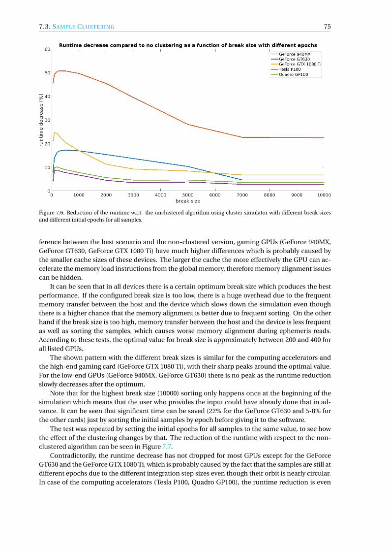
7.3. SAMPLE CLUSTERING 75
Figure 7.6: Reduction of the runtime w.r.t. the unclustered algorithm using cluster simulator with different break sizesand different initial epochs for all samples.
ference between the best scenario and the non-clustered version, gaming GPUs (GeForce 940MX,GeForce GT630, GeForce GTX 1080 Ti) have much higher differences which is probably caused bythe smaller cache sizes of these devices. The larger the cache the more effectively the GPU can ac-celerate the memory load instructions from the global memory, therefore memory alignment issuescan be hidden.
It can be seen that in all devices there is a certain optimum break size which produces the bestperformance. If the configured break size is too low, there is a huge overhead due to the frequentmemory transfer between the host and the device which slows down the simulation even thoughthere is a higher chance that the memory alignment is better due to frequent sorting. On the otherhand if the break size is too high, memory transfer between the host and the device is less frequentas well as sorting the samples, which causes worse memory alignment during ephemeris reads.According to these tests, the optimal value for break size is approximately between 200 and 400 forall listed GPUs.
The shown pattern with the different break sizes is similar for the computing accelerators andthe high-end gaming card (GeForce GTX 1080 Ti), with their sharp peaks around the optimal value.For the low-end GPUs (GeForce 940MX, GeForce GT630) there is no peak as the runtime reductionslowly decreases after the optimum.
Note that for the highest break size (10000) sorting only happens once at the beginning of thesimulation which means that the user who provides the input could have already done that in ad-vance. It can be seen that significant time can be saved (22% for the GeForce GT630 and 5-8% forthe other cards) just by sorting the initial samples by epoch before giving it to the software.
The test was repeated by setting the initial epochs for all samples to the same value, to see howthe effect of the clustering changes by that. The reduction of the runtime with respect to the non-clustered algorithm can be seen in Figure 7.7.
Contradictorily, the runtime decrease has not dropped for most GPUs except for the GeForceGT630 and the GeForce GTX 1080 Ti, which is probably caused by the fact that the samples are still atdifferent epochs due to the different integration step sizes even though their orbit is nearly circular.In case of the computing accelerators (Tesla P100, Quadro GP100), the runtime reduction is even
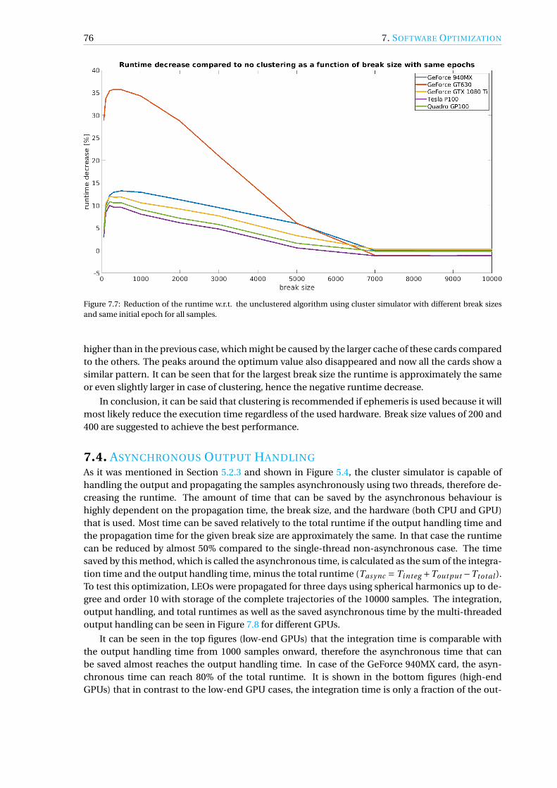
76 7. SOFTWARE OPTIMIZATION
Figure 7.7: Reduction of the runtime w.r.t. the unclustered algorithm using cluster simulator with different break sizesand same initial epoch for all samples.
higher than in the previous case, which might be caused by the larger cache of these cards comparedto the others. The peaks around the optimum value also disappeared and now all the cards show asimilar pattern. It can be seen that for the largest break size the runtime is approximately the sameor even slightly larger in case of clustering, hence the negative runtime decrease.
In conclusion, it can be said that clustering is recommended if ephemeris is used because it willmost likely reduce the execution time regardless of the used hardware. Break size values of 200 and400 are suggested to achieve the best performance.
7.4. ASYNCHRONOUS OUTPUT HANDLING
As it was mentioned in Section 5.2.3 and shown in Figure 5.4, the cluster simulator is capable ofhandling the output and propagating the samples asynchronously using two threads, therefore de-creasing the runtime. The amount of time that can be saved by the asynchronous behaviour ishighly dependent on the propagation time, the break size, and the hardware (both CPU and GPU)that is used. Most time can be saved relatively to the total runtime if the output handling time andthe propagation time for the given break size are approximately the same. In that case the runtimecan be reduced by almost 50% compared to the single-thread non-asynchronous case. The timesaved by this method, which is called the asynchronous time, is calculated as the sum of the integra-tion time and the output handling time, minus the total runtime (Tas ync = Ti nteg +Tout put −Ttot al ).To test this optimization, LEOs were propagated for three days using spherical harmonics up to de-gree and order 10 with storage of the complete trajectories of the 10000 samples. The integration,output handling, and total runtimes as well as the saved asynchronous time by the multi-threadedoutput handling can be seen in Figure 7.8 for different GPUs.
It can be seen in the top figures (low-end GPUs) that the integration time is comparable withthe output handling time from 1000 samples onward, therefore the asynchronous time that canbe saved almost reaches the output handling time. In case of the GeForce 940MX card, the asyn-chronous time can reach 80% of the total runtime. It is shown in the bottom figures (high-endGPUs) that in contrast to the low-end GPU cases, the integration time is only a fraction of the out-

7.5. EPHEMERIS RETRIEVAL 77
Figure 7.8: Integration, output handling, total runtimes and the saved asynchronous time of LEO propagations withstep storage on low-end GPUs (top left: GeForce 940MX, top right: GeForce GT630) and on high-end GPUs (bottomleft: GeForce GTX 1080 Ti, bottom right: Quadro GP100).
put handling time, therefore the asynchronous time is much less as a ratio of the total runtime thanin the low-end GPU simulations. It can also be seen that the total runtime is the lowest for theGeForce GTX 1080 Ti despite of having a much higher integration time than the scientific accelera-tor (Quadro GP100), which is caused by the faster CPU (Intel Xeon Gold 5120) that is connected tothe gaming card. In conclusion, if output handling dominates the total simulation time, the highercomputing power of the high-end GPUs is hidden, therefore low-end GPU simulations can producesimilar runtimes as high-end GPU simulations.
7.5. EPHEMERIS RETRIEVALSome force models, such as the third-body perturbation or SRP, require ephemeris retrieval dur-ing their evaluation. Since this function evaluation takes place at every intermediate stage of anintegration step, it is critical to optimize it to be able to see significant performance improvement.
To access any data that is not already in GPU memory is highly time consuming due to thememory bottleneck of the PCIe bus, therefore it is not possible to use already available librariesdeveloped for CPUs, such as SPICE or CALCEPH, in the computation of the ephemeris. The solutionto this problem is to transfer all the necessary data to the GPU memory once, at the beginning ofthe simulation, and retrieve the ephemeris on the device during the simulation. Most modern GPUshave large enough global memory to store a complete ephemeris file which can be up to several GB.However if the simulation period is known in advance it is highly beneficial to store only the requireddata in device memory, which is the method implemented in CUDAjectory.
If only the required data is transferred to the GPU instead of a whole ephemeris file, up to 3%better performance can be achieved depending on the device and the selected time periods andephemeris files. The order of the bodies in the ephemeris data could play a role in the efficientcaching during the evaluation of the positions of these bodies, however tests showed that the exe-cution time does not change by altering the order of the bodies.
The number of ephemeris evaluations from the Chebyshev polynomials can be significantly re-
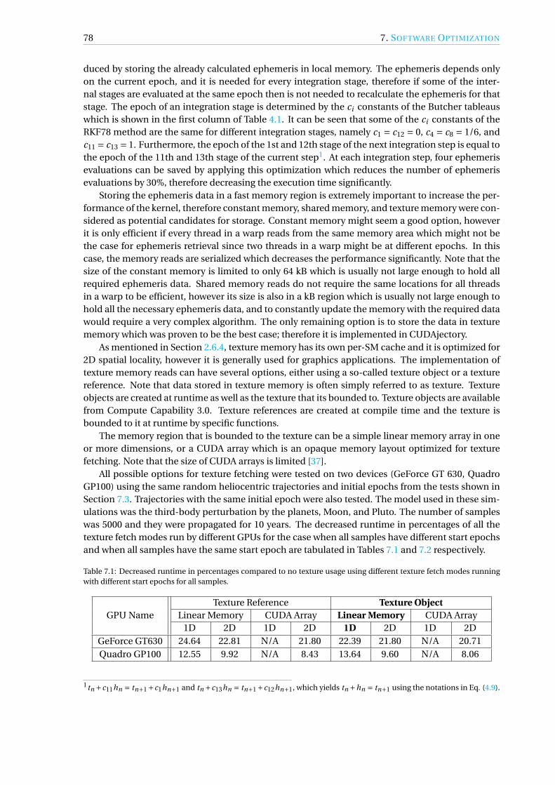
78 7. SOFTWARE OPTIMIZATION
duced by storing the already calculated ephemeris in local memory. The ephemeris depends onlyon the current epoch, and it is needed for every integration stage, therefore if some of the inter-nal stages are evaluated at the same epoch then is not needed to recalculate the ephemeris for thatstage. The epoch of an integration stage is determined by the ci constants of the Butcher tableauswhich is shown in the first column of Table 4.1. It can be seen that some of the ci constants of theRKF78 method are the same for different integration stages, namely c1 = c12 = 0, c4 = c8 = 1/6, andc11 = c13 = 1. Furthermore, the epoch of the 1st and 12th stage of the next integration step is equal tothe epoch of the 11th and 13th stage of the current step1. At each integration step, four ephemerisevaluations can be saved by applying this optimization which reduces the number of ephemerisevaluations by 30%, therefore decreasing the execution time significantly.
Storing the ephemeris data in a fast memory region is extremely important to increase the per-formance of the kernel, therefore constant memory, shared memory, and texture memory were con-sidered as potential candidates for storage. Constant memory might seem a good option, howeverit is only efficient if every thread in a warp reads from the same memory area which might not bethe case for ephemeris retrieval since two threads in a warp might be at different epochs. In thiscase, the memory reads are serialized which decreases the performance significantly. Note that thesize of the constant memory is limited to only 64 kB which is usually not large enough to hold allrequired ephemeris data. Shared memory reads do not require the same locations for all threadsin a warp to be efficient, however its size is also in a kB region which is usually not large enough tohold all the necessary ephemeris data, and to constantly update the memory with the required datawould require a very complex algorithm. The only remaining option is to store the data in texturememory which was proven to be the best case; therefore it is implemented in CUDAjectory.
As mentioned in Section 2.6.4, texture memory has its own per-SM cache and it is optimized for2D spatial locality, however it is generally used for graphics applications. The implementation oftexture memory reads can have several options, either using a so-called texture object or a texturereference. Note that data stored in texture memory is often simply referred to as texture. Textureobjects are created at runtime as well as the texture that its bounded to. Texture objects are availablefrom Compute Capability 3.0. Texture references are created at compile time and the texture isbounded to it at runtime by specific functions.
The memory region that is bounded to the texture can be a simple linear memory array in oneor more dimensions, or a CUDA array which is an opaque memory layout optimized for texturefetching. Note that the size of CUDA arrays is limited [37].
All possible options for texture fetching were tested on two devices (GeForce GT 630, QuadroGP100) using the same random heliocentric trajectories and initial epochs from the tests shown inSection 7.3. Trajectories with the same initial epoch were also tested. The model used in these sim-ulations was the third-body perturbation by the planets, Moon, and Pluto. The number of sampleswas 5000 and they were propagated for 10 years. The decreased runtime in percentages of all thetexture fetch modes run by different GPUs for the case when all samples have different start epochsand when all samples have the same start epoch are tabulated in Tables 7.1 and 7.2 respectively.
Table 7.1: Decreased runtime in percentages compared to no texture usage using different texture fetch modes runningwith different start epochs for all samples.
GPU NameTexture Reference Texture Object
Linear Memory CUDA Array Linear Memory CUDA Array1D 2D 1D 2D 1D 2D 1D 2D
GeForce GT630 24.64 22.81 N/A 21.80 22.39 21.80 N/A 20.71Quadro GP100 12.55 9.92 N/A 8.43 13.64 9.60 N/A 8.06
1tn +c11hn = tn+1+c1hn+1 and tn +c13hn = tn+1+c12hn+1, which yields tn +hn = tn+1 using the notations in Eq. (4.9).

7.6. GRAVITY MODEL 79
Table 7.2: Decreased runtime in percentages compared to no texture usage using different texture fetch modes runningwith the same start epoch for all samples.
GPU NameTexture Reference Texture Object
Linear Memory CUDA Array Linear Memory CUDA Array1D 2D 1D 2D 1D 2D 1D 2D
GeForce GT630 13.21 11.17 7.77 10.42 11.09 10.07 8.34 9.36Quadro GP100 10.49 8.58 5.39 8.48 11.48 7.90 5.06 7.85
It is shown in the tables that the performance increment is extremely significant due to the fasteraccesses to the ephemeris data. It can be seen that due to the limited size of CUDA arrays (65536)the total ephemeris data could not fit in them, therefore those records are not applicable for the casewhere the samples had different start epochs. In the other case, when the samples have the samestart epoch the ephemeris data could fit into texture memory using CUDA arrays. The CUDA arraysare not as efficient as the simple linear memory, not even in the 2D case which they are optimized to.It can be seen that the CUDA array is clearly more efficient in 2D, whereas the linear memory is moreefficient in 1D. Texture references are more effective for the older gaming card (GeForce GT630) thanfor the newer computing accelerator card (Quadro GP100). Texture objects on the other hand aremore efficient for the new card. Due to this fact and that they are more robust in usage than texturereferences, the texture object which is bound to a 1D linear memory array was chosen in the finalimplementation.
7.6. GRAVITY MODEL
The most simple optimization method for the gravity models is to transfer the constant coefficients(spherical harmonics coefficients, point mascon positions and gravitational parameters) into a fastmemory region of the GPU. Since these coefficients do not change during the simulation it is ev-ident to keep them in constant memory. However, the size of the constant memory is only 64 kBin all CUDA-capable devices, which is not necessarily large enough to hold all the variables of thegravity model. In CUDAjectory a buffer of 60 kB is reserved in the constant memory region specifi-cally to contain gravity model data, which is enough to contain a spherical harmonics model up todegree and order 86 and a point mascon model using 1920 mascons, which is equivalent to degreeand order 39 resolution of the spherical harmonics model. If the user configures a gravity modelwith higher fidelity, the coefficients are stored in global memory. Extensive tests showed that onlya maximum of 1-2% performance gain can be achieved by using constant memory for the gravitymodel. This value may seem low, which is caused by the fact that the compiler can optimize if avariable is read only in a kernel, therefore placing it in constant memory does not have a huge ef-fect in this case. The performance comparison between the two implemented gravity models canbe seen in Figure 7.9. This performance test was conducted on different GPUs measuring the timespent only in the acceleration evaluation functions.
It is shown in the figure that the performance difference between the two models is clearly de-pendent on the hardware that is used. The two GeForce cards are gaming GPUs, therefore they havemuch less double-precision throughput than the Tesla and Quadro cards, which are computing ac-celerators. It can be seen that the spherical harmonics model is 1.2-9.5 times faster than the pointmascon model for every case. Three distinguished lines can be seen in the figure for each GPU be-cause the number of mascons is the same for different resolutions (e.g. 1920 mascons for degreeand order 33, 35, and 39), whereas the number of coefficients increases by higher resolution for thespherical harmonics model. For the computing accelerators (Tesla, Quadro) the speedup decreaseswith increasing fidelity for less than degree and order 40 because these cards have extremely largethroughput (4-5 TFLOP/s) and they cannot use their full computing capacity if the resolution of the

80 7. SOFTWARE OPTIMIZATION
Figure 7.9: Runtime comparison between the point mascon and spherical harmonics gravity models using different fi-delity and GPUs.
gravity model is low. This is not the case for the gaming cards which have an approximately constantspeedup for every fidelity.
The main reason behind the huge difference in performance between the two models is thatthe point mascon model requires a large number of memory load instructions since the positionsand the gravitational parameters of the mascons are stored in constant memory. Although the pointmascon model requires much less arithmetic operations, the overall performance is worse due tothe fact that the latency for a memory load operation is usually an order of magnitude higher thanfor an arithmetic operation.
A metric called Compute to Global Memory Access (CGMA), which is defined as the ratio offloating-point operations to global memory access operations, can show the reason for this largeperformance difference between the two models. Usually, the higher the CGMA the better the per-formance because of this latency difference between the memory load and arithmetic operations.However the CGMA ratio does not tell us the individual values of the floating-point operations orthe memory access operations, therefore the performance of two kernels with the same CGMA canbe different. The CGMA of the two gravity models using different fidelity can be seen in Figure 7.10.Note that the memory access operations were counted as an access to a spherical harmonics coef-ficient or point mascon data regardless of being stored in global or constant memory.
It can be seen in the figure that the spherical harmonics model has a much higher CGMA thanthe point mascon model, which explains its better performance. The CGMA is slowly decreasingwith increasing resolution for the spherical harmonics model due to the higher number of mem-ory loads compared to the arithmetic instructions, whereas it stays constant for the point masconmodel. The ratio of floating-point operations and memory accesses of the two models can be seenin Figure 7.11.
It is shown in the figure that the point mascon model has approximately half to three quartersthe number of floating-point operations and 2.5-3.5 times more memory access instructions thanthe spherical harmonics model. Because the latency of one memory access is at least 10 times largerthan of a floating-point operation, it is evident that the performance of the point mascon modelwill be worse because it is not possible to hide this latency by increasing the number of threads orinstruction level parallelism.

7.6. GRAVITY MODEL 81
Figure 7.10: Compute to Global Memory Access (CGMA) of the spherical harmonics and point mascon gravity modelsusing different fidelity.
Figure 7.11: Ratio of floating-point operations (top) and memory accesses (bottom) of the point mascon and sphericalharmonics gravity models for different fidelity.
A possible option to optimize the point mascon model would be to use dynamic parallelism tocalculate the contribution of each mascon to the total acceleration in parallel, and use e.g. parallelreduction to sum each partial acceleration. Parallel reduction can sum the elements of a vector us-ing less addition operation using nested parallelism. Reduce algorithms using dynamic parallelismare implemented in several libraries such as NVIDIA’s Thrust or the CUB library [38, 39]. However, inorder to calculate the contribution by each mascon using dynamic parallelism, all the accelerationshave to be stored in global memory because a kernel cannot be launched by passing variables that

82 7. SOFTWARE OPTIMIZATION
reside in local memory. Therefore, the acceleration caused by each mascon of each sample has tobe stored globally, which could be several GBs for a high-fidelity mascon model and a large numberof samples. It may be faster to calculate the accelerations with this method however, they have tobe accessed again by the parallel reduction algorithm and as shown, the latency of global memoryaccesses is much higher than that of arithmetic operations. Tests showed that regardless of usingthe Thrust or the CUB library, dynamic parallelism proves to be inefficient in optimizing the pointmascon gravity model.
In conclusion, it is not recommended to use the point mascon model in CUDAjectory if the pri-mary objective is efficiency. However, for GPU-assisted CPU propagation, the point mascon modelcould be the better option.

8 SOFTWARE PERFORMANCE
In this chapter, performance tests will be described which aim to represent how effective the GPUexecution is compared to a single-core CPU version using CUDAjectory. The tests will show cer-tain configurations and compare the performance using different number of samples and differentGPUs. The software is capable of measuring the total runtime, the integration time, and the out-put handling time, although most of the presented comparisons will include the integration time,because that part of the execution is done on the GPUs. Whenever the total runtime or the outputhandling time is included it will be emphasized. The tests were repeated several times and the pre-sented values yielded as the average of these simulations. The speedups that will be shown in thediagrams are simply calculated by the ratio of the runtimes of the sequential CPU version and theparallel GPU version. The simulations were tested on different CPUs and the fastest of these runswere chosen for comparison, which can differ from case to case. Note that the data for high sam-ple numbers is the result of extrapolation for the CPUs and low-end GPUs, because it would take asignificant amount of time to run the total simulations. Extrapolation is a valid method to get thesenumbers since the runtimes for CPUs scale linearly with increasing sample count, as well as forGPUs after the number of samples reached the point where latency hiding is not effective anymore.
8.1. TWO-BODY PROBLEMThe performance of the GPU version was tested integrating the unperturbed two-body problemcase for near-circular LEOs. The propagation time was set to five days and 10−12 was used as relativeand absolute integration tolerance. The speedups for different number of samples compared to theIntel Core i7-4970 CPU can be seen in Figure 8.1.
Figure 8.1: Speedup as a function of sample numbers between CPU and GPU runs integrating the two-body problem.
It can be seen that the two low-end GPUs (GeForce 940MX, GeForce GT630) barely bring anyspeedups, while the high-end gaming GPU (GeForce GTX 1080 Ti) and the computing accelerators(Tesla P100, Quadro GP100) produce speedups of maximum 18 and 24 respectively. For lower num-ber of samples, as expected, the speedup is well below one, and it gradually increases until a certainthreshold when the GPUs saturate. From that point the speedup is approximately constant becausethe runtimes of the GPUs also increase linearly. For this particular case the threshold for the low-endcards is approximately 1000 samples, for the GeForce GTX 1080 Ti is around 10000 samples, and forthe computing accelerators it is around 50000.
83

84 8. SOFTWARE PERFORMANCE
8.2. THIRD-BODY PERTURBATIONHeliocentric orbits were propagated using all the planets, the Moon, and Pluto as perturbing bodiesfor 10 years. Two different runs were simulated, one where all the samples have the same initialepoch, and one where the samples have different initial epochs. The speedups of these two simu-lations comparing the various GPU and the CPU (Intel Core i7-4970) cases for different number ofsamples can be seen in Figure 8.2.
Figure 8.2: Speedup as a function of sample numbers between CPU and GPU runs simulating heliocentric orbits usingthird-body perturbation of all the planets, the Moon, and Pluto working with the same initial epochs (top) and differentinitial epochs (bottom) for all samples.
A similar pattern can be seen in the figure compared to the two-body case. For lower samplenumbers the speedup is very small and it increases until a threshold, after which it stays approxi-mately constant. The difference between the speedups of the cases with the same epochs and dif-ferent epochs case can reach a factor of 10 for the high-end GPUs, which is caused by the memoryloading issue that was explained in Section 7.3. The runtime increment by changing from cases withthe same epochs to cases with different epochs can be seen in Figure 8.3.

8.2. THIRD-BODY PERTURBATION 85
Figure 8.3: Runtime increment in percentages from same epochs to different epochs case simulating heliocentric orbitswith third-body perturbation of all planets, the Moon, and Pluto.
It is shown in Figure 8.3 that the increment changes with different numbers of samples and dif-ferent GPUs and it can even reach 50%. The runtime of the CPU cases only change 1-2%, hence thelarge difference in the speedups. Note that these results were produced using the cluster simulatorwith a break size of 200 for a specific case, therefore the increments can change for different con-figurations. This study was intended to show that by changing the initial epochs of the samples theruntime is significantly influenced on the GPU which is not the case on the CPU.
A barycentric case of similar orbits was simulated using SRP without eclipse detection usingdifferent initial epochs for all samples. The speedups of these simulations compared to the IntelCore i7-4970 CPU can be seen in Figure 8.4.
Figure 8.4: Speedup as a function of sample numbers between CPU and GPU runs using barycentric simulation and SRPwithout eclipse detection.
The values shown in Figure 8.4 are very similar to the heliocentric case (bottom of Figure 8.2).The runtimes are increased by 4-5% for all cases due to the addition of the SRP to the model.

86 8. SOFTWARE PERFORMANCE
8.3. SPHERICAL HARMONICSEarth-centric LEOs were propagated using the spherical harmonics model up to degree and order 10for three days. The speedups compared to the Intel Core i7-6820HQ CPU are presented in Figure 8.5.
Figure 8.5: Speedup as a function of sample numbers between CPU and GPU runs using spherical harmonics up to degreeand order 10.
It can be seen in the figure that the speedups are much higher and can almost reach 150 atmaximum. This is caused by the fact that the evaluation of the accelerations caused by the spheri-cal harmonics model require a large number of arithmetic calculations and therefore the executionis more core-intensive than memory-intensive. Because of this, the throughput of the simulationhas significantly increased, which results in higher speedups compared to the CPU version. Thelarger difference between the performance of the gaming cards and the computing accelerators isalso evident in this test. Computing accelerators have approximately 10 times the peak throughputin double-precision calculations than gaming cards, hence the large difference between the perfor-mance of these GPU types. Although all GPUs are still under-utilized compared to their peak perfor-mance, this test shows the substantial difference in performance between the scientific acceleratorsand the gaming cards.
8.4. HIGHLY ELLIPTICAL ORBITSIn this example, different types of orbits from circular to highly elliptical with Earth at center werepropagated with the following Keplerian elements:
t0 ∈ [−11000 MJD2000,16000 MJD2000]
a ∈ [6700 km,200000 km]
e ∈ [0,0.97]
i ∈ [0,90]
Ω ∈ [0,360]
ω ∈ [0,360]
θ ∈ [0,360]
(8.1)
The dynamical model used in this propagation was the third-body perturbation by the Moon andthe Sun. The samples were propagated for one year. Since the initial epochs and Keplerian elements
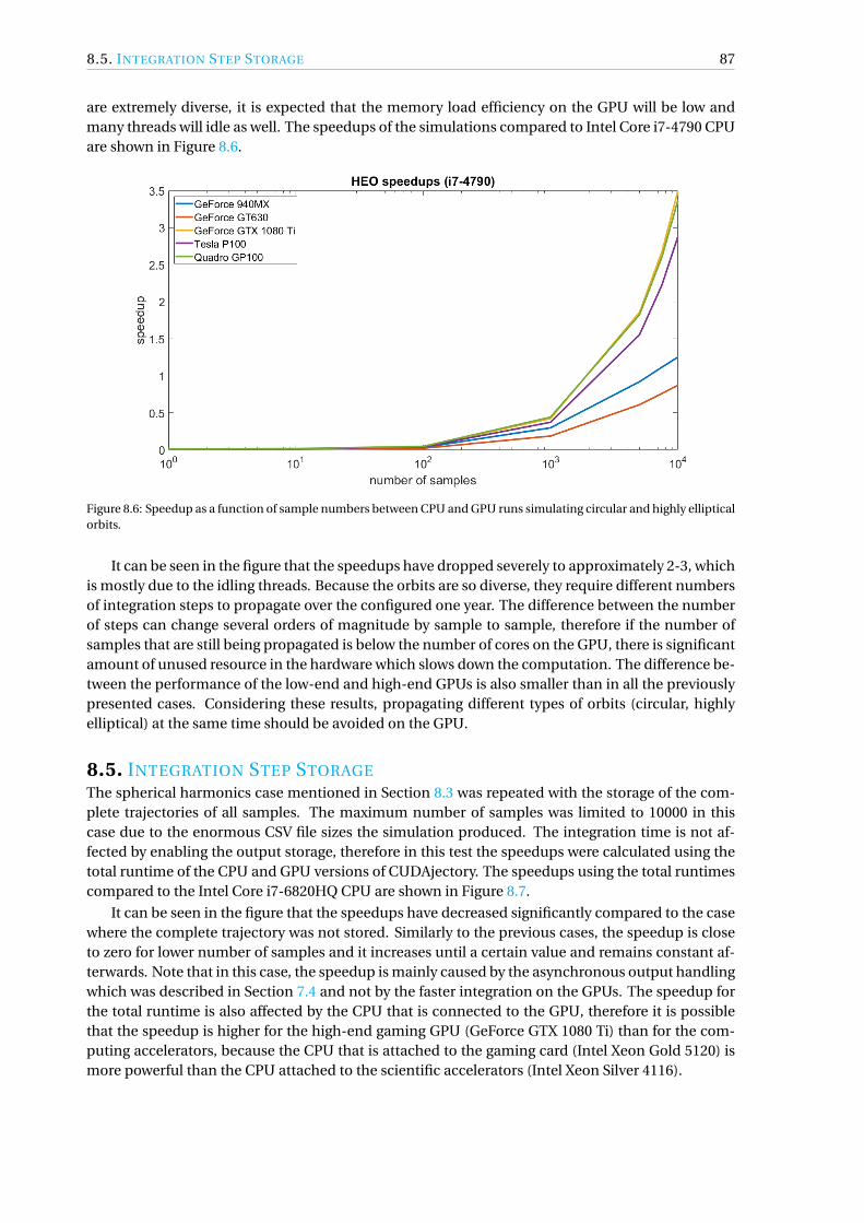
8.5. INTEGRATION STEP STORAGE 87
are extremely diverse, it is expected that the memory load efficiency on the GPU will be low andmany threads will idle as well. The speedups of the simulations compared to Intel Core i7-4790 CPUare shown in Figure 8.6.
Figure 8.6: Speedup as a function of sample numbers between CPU and GPU runs simulating circular and highly ellipticalorbits.
It can be seen in the figure that the speedups have dropped severely to approximately 2-3, whichis mostly due to the idling threads. Because the orbits are so diverse, they require different numbersof integration steps to propagate over the configured one year. The difference between the numberof steps can change several orders of magnitude by sample to sample, therefore if the number ofsamples that are still being propagated is below the number of cores on the GPU, there is significantamount of unused resource in the hardware which slows down the computation. The difference be-tween the performance of the low-end and high-end GPUs is also smaller than in all the previouslypresented cases. Considering these results, propagating different types of orbits (circular, highlyelliptical) at the same time should be avoided on the GPU.
8.5. INTEGRATION STEP STORAGEThe spherical harmonics case mentioned in Section 8.3 was repeated with the storage of the com-plete trajectories of all samples. The maximum number of samples was limited to 10000 in thiscase due to the enormous CSV file sizes the simulation produced. The integration time is not af-fected by enabling the output storage, therefore in this test the speedups were calculated using thetotal runtime of the CPU and GPU versions of CUDAjectory. The speedups using the total runtimescompared to the Intel Core i7-6820HQ CPU are shown in Figure 8.7.
It can be seen in the figure that the speedups have decreased significantly compared to the casewhere the complete trajectory was not stored. Similarly to the previous cases, the speedup is closeto zero for lower number of samples and it increases until a certain value and remains constant af-terwards. Note that in this case, the speedup is mainly caused by the asynchronous output handlingwhich was described in Section 7.4 and not by the faster integration on the GPUs. The speedup forthe total runtime is also affected by the CPU that is connected to the GPU, therefore it is possiblethat the speedup is higher for the high-end gaming GPU (GeForce GTX 1080 Ti) than for the com-puting accelerators, because the CPU that is attached to the gaming card (Intel Xeon Gold 5120) ismore powerful than the CPU attached to the scientific accelerators (Intel Xeon Silver 4116).

88 8. SOFTWARE PERFORMANCE
Figure 8.7: Speedup as a function of sample numbers between CPU and GPU runs using spherical harmonics up to degreeand order 10 and storing every integration step.
8.6. CONCLUSIONSTo summarize the results of these performance tests, it can be concluded that the highest speedupsof the GPU simulations compared to the single core CPU version can be achieved if the number ofsamples is large enough to reach the point where the GPUs cannot hide more latency. This valuedepends on the hardware and the configuration but for modern high-end GPUs it is approximatelybetween 10000 and 100000.
For simulations that include ephemeris calculations, higher speedups can be achieved if all thesamples have the same initial epoch. This is caused by the more efficient memory loading, whichoccurs if all threads within a warp have to access the same memory locations for the ephemerisdata. Therefore the caching of these memory loads can be much more efficient compared to thecase when the threads require different ephemeris data. Obviously, this problem is not present ifthe samples are propagated sequentially on a single CPU.
It is desired to propagate similar types of orbits on a GPU, because if some threads in a warp havealready finished propagation they will idle, therefore the number of inactive threads will increase. Ahigh number of inactive threads will lead to a serious performance decrease.
If the dynamical model of the propagation is core-intensive, in other words a large number ofarithmetic calculations is required without many memory load instructions, the highest speedupscan be achieved. The difference between the performance of scientific accelerators and gamingcards is also largest while running these simulations.
If the simulation is I/O-intensive, i.e. integration step storage is enabled, the achieved speedup(comparing the total runtimes of the GPU and CPU simulations) is extremely small compared to thecase when the full trajectory is not saved, even though the integration time is still much smaller ona GPU.

9 STUDY CASES
This chapter will describe study cases which use CUDAjectory to calculate the trajectories of manysamples and draw conclusions based on the produced data. The similarity of the results will be com-pared to calculations done by other software available at ESOC, namely FastProp and SNAPPshot.These programs were parallelized using MATLAB’s Parallel Computing Toolbox and OpenMP, there-fore they can be run on single- or multi-core CPUs. A performance comparison of CUDAjectory andthese other software will be carried out, however this should be taken with great care because thetwo software may produce similar results, but they were designed for different purposes.
9.1. BEPICOLOMBO UPPER STAGE DISPOSALBepiColombo is a joint mission of the European Space Agency (ESA) and the Japan Aerospace Explo-ration Agency (JAXA) to visit Mercury. The mission’s primary objective is to study and characterizethe planet’s magnetic field, magnetosphere, as well as its interior and surface structure. The mis-sion consists of two spacecrafts: the Mercury Planetary Orbiter (MPO) to map the planet, and theMercury Magnetospheric Orbiter (MMO) to explore its magnetosphere. The satellite was launchedon 20 October 2018 by an Ariane 5 launcher from Guiana Space Centre in Kourou, French Guiana.The arrival at Mercury is planned for December 2025 after nine planetary flybys, one of Earth, twoof Venus, and six of Mercury [40].
The disposal of the upper stage of the launch vehicle has been studied to fulfill space debrismitigation requirements set by the International Organization for Standardization (ISO). ESA hasset requirements in re-entry casualty risk acceptance and assessment which have to be compliedwith to approve the mission. According to the ECSS-U-AS-10C / ISO 24113:2011 requirement, themaximum acceptable casualty risk on ground of a controlled or uncontrolled re-entry of a space-craft, launch vehicle stage, etc. can be 10−4 [41].
The initial states are based on dispersion data, which is established by the specifications of theAriane 5 launcher determined by Arianespace in the so-called Kourou frozen frame after the pas-sivization of the upper stage. The data was provided for the entire launch window, which is 42 daysbetween 18 Oct 2018 and 28 Nov 2018. The dispersed state of the upper stage had to be transformedinto the J2000 reference frame a priori, which can be used by CUDAjectory. The initial heliocentricKeplerian elements of the states are within the following intervals:
a ∈ [1.38 AU,1.48 AU]
e ∈ [0.37,0.40]
i ∈ [22.7,24.7]
Ω ∈ [−0.9,6]
ω ∈ [82.3,109.4]
θ ∈ [−57.7,−48.8]
(9.1)
The number of samples per each launch window was 10000, which made the total sample countequal to 420000, which is perfectly suitable for a GPU. The simulation period was set to 100 years.The dynamical model of this analysis included the perturbation by all the planets, Pluto, and theMoon, the J2-term of the gravity field of a planet if the sample is inside its SOI, and SRP withouteclipse condition checks. The ephemeris model used was the JPL DE422 model. Collision and SOIcrossing checks were enabled. The relative and absolute integration tolerance was set to 10−12. Thecenter of propagation was switched to a planetary body if the satellite was inside its SOI. The clustersimulator with a break size of 300 was used for all simulations.
89
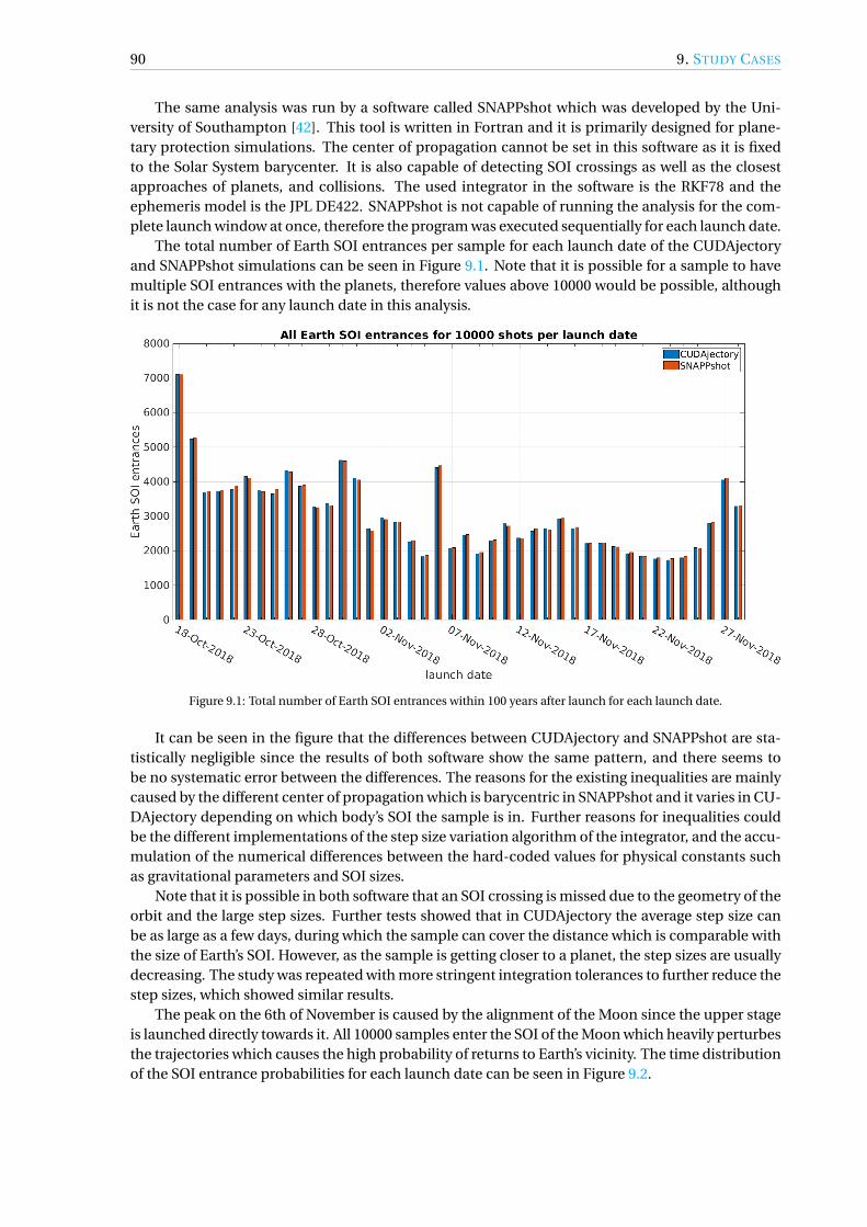
90 9. STUDY CASES
The same analysis was run by a software called SNAPPshot which was developed by the Uni-versity of Southampton [42]. This tool is written in Fortran and it is primarily designed for plane-tary protection simulations. The center of propagation cannot be set in this software as it is fixedto the Solar System barycenter. It is also capable of detecting SOI crossings as well as the closestapproaches of planets, and collisions. The used integrator in the software is the RKF78 and theephemeris model is the JPL DE422. SNAPPshot is not capable of running the analysis for the com-plete launch window at once, therefore the program was executed sequentially for each launch date.
The total number of Earth SOI entrances per sample for each launch date of the CUDAjectoryand SNAPPshot simulations can be seen in Figure 9.1. Note that it is possible for a sample to havemultiple SOI entrances with the planets, therefore values above 10000 would be possible, althoughit is not the case for any launch date in this analysis.
Figure 9.1: Total number of Earth SOI entrances within 100 years after launch for each launch date.
It can be seen in the figure that the differences between CUDAjectory and SNAPPshot are sta-tistically negligible since the results of both software show the same pattern, and there seems tobe no systematic error between the differences. The reasons for the existing inequalities are mainlycaused by the different center of propagation which is barycentric in SNAPPshot and it varies in CU-DAjectory depending on which body’s SOI the sample is in. Further reasons for inequalities couldbe the different implementations of the step size variation algorithm of the integrator, and the accu-mulation of the numerical differences between the hard-coded values for physical constants suchas gravitational parameters and SOI sizes.
Note that it is possible in both software that an SOI crossing is missed due to the geometry of theorbit and the large step sizes. Further tests showed that in CUDAjectory the average step size canbe as large as a few days, during which the sample can cover the distance which is comparable withthe size of Earth’s SOI. However, as the sample is getting closer to a planet, the step sizes are usuallydecreasing. The study was repeated with more stringent integration tolerances to further reduce thestep sizes, which showed similar results.
The peak on the 6th of November is caused by the alignment of the Moon since the upper stageis launched directly towards it. All 10000 samples enter the SOI of the Moon which heavily perturbesthe trajectories which causes the high probability of returns to Earth’s vicinity. The time distributionof the SOI entrance probabilities for each launch date can be seen in Figure 9.2.

9.1. BEPICOLOMBO UPPER STAGE DISPOSAL 91
Figure 9.2: Time distribution of Earth SOI entrance probabilities for each launch date.
It is shown in the figure that the upper stage does not cross the SOI of Earth within the first 10-15 years after launch, which shows that there are no short-term resonances with Earth. The largerprobabilities of an SOI crossing are present for the earlier and the latest launch dates after 25-35years. A small gap can be seen at the 25-35 line at the first few days of November. Launching on thesedates, the first SOI crossing happens approximately 50 years after departure. It can be deductedfrom this plot that the probability of the SOI entrance is dropping after a larger peak, which meansthat the upper stage does not frequently return more than once to the vicinity of Earth. This iscaused by the heavy perturbation during the first encounter with Earth, which changes the orbitalelements of the sample significantly. The number of collisions with Earth produced by CUDAjectoryand SNAPPshot can be seen in Figure 9.3.
Figure 9.3: Number of collisions with Earth within 100 years after launch for each launch date.

92 9. STUDY CASES
Figure 9.3 shows that there are larger differences between the two software compared to the SOIentrance values, which is caused by the fact that the number of collisions is much smaller than thenumber of SOI entrances. However, for larger collision numbers the relative difference is smaller. Itcan be seen that for the first five launch dates (except the fourth) the number of collisions is muchhigher than for the rest of launch dates, which is caused by a resonance that is present at those tra-jectories. The probability of SOI crossings was also highest at these dates, hence the larger numberof impacts with Earth. At the last launch dates there are no collisions detected although the proba-bility of an SOI crossing was higher. This shows that there seems to be no direct connection betweenthe probability of SOI entrances and the probability of collisions. The time distribution of the Earthcollision probability is shown in Figure 9.4.
Figure 9.4: Time distribution of the probability of Earth collisions within 100 years after launch for each launch date.
It can be seen in the figure that the probability for collisions is at a maximum of 0.3%. Furtheranalysis of the exact location of the returns and a break-up analysis would be needed to calculatethe on-ground casualty risk to check if it meets the requirement, which was not done in this disposalanalysis. The figure shows that no collisions occur within the first 25 years after launch, thereforethere are no short-term resonances with Earth. There is a larger group of collisions between 2043and 2048, most of which are happening in 2044, 2045 and 2046. The resonances with Earth for thesedates are 26:15, 27:16, and 28:17 respectively, which are consistent with the initial semi-major axes ofthese orbits. The colliding trajectories launched between 18-20 October are in a 28:17 resonance, on22 October are in a 27:16 resonance, and on 21 October are in a 26:15 resonance with Earth. Figure9.4 also shows that at other dates, the probability of a collision is close to zero therefore negligible.
After the validation of the results, the performance of CUDAjectory and SNAPPshot was com-pared. Note that SNAPPshot is not capable of running the analysis for the total launch window atonce, therefore only one launch date (10000 samples) was selected for the performance comparisonwith CUDAjectory. To make a fair comparison, SNAPPshot was executed on the servers of ESOC us-ing the parallel CPU version of the software implemented in OpenMP. The simulation runtimes forthe different setups are tabulated in Table 9.1.
It can be seen that the simulation times of CUDAjectory run on the different GPUs are compa-rable with the SNAPPshot simulation using 48 cores, which is approximately equal to a speedup of35-40 compared with a single-core simulation. It can be also seen that the runtimes using the differ-ent high-end GPUs do not significantly differ due to the high output handling times. The speedupof the high-end GPU runs compared to the single-core CUDAjectory CPU version is in line with
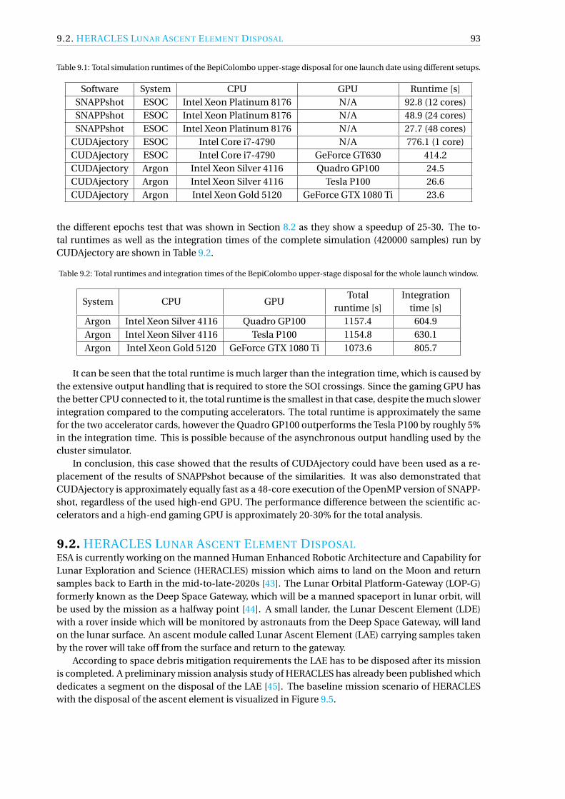
9.2. HERACLES LUNAR ASCENT ELEMENT DISPOSAL 93
Table 9.1: Total simulation runtimes of the BepiColombo upper-stage disposal for one launch date using different setups.
Software System CPU GPU Runtime [s]SNAPPshot ESOC Intel Xeon Platinum 8176 N/A 92.8 (12 cores)SNAPPshot ESOC Intel Xeon Platinum 8176 N/A 48.9 (24 cores)SNAPPshot ESOC Intel Xeon Platinum 8176 N/A 27.7 (48 cores)
CUDAjectory ESOC Intel Core i7-4790 N/A 776.1 (1 core)CUDAjectory ESOC Intel Core i7-4790 GeForce GT630 414.2CUDAjectory Argon Intel Xeon Silver 4116 Quadro GP100 24.5CUDAjectory Argon Intel Xeon Silver 4116 Tesla P100 26.6CUDAjectory Argon Intel Xeon Gold 5120 GeForce GTX 1080 Ti 23.6
the different epochs test that was shown in Section 8.2 as they show a speedup of 25-30. The to-tal runtimes as well as the integration times of the complete simulation (420000 samples) run byCUDAjectory are shown in Table 9.2.
Table 9.2: Total runtimes and integration times of the BepiColombo upper-stage disposal for the whole launch window.
System CPU GPUTotal
runtime [s]Integration
time [s]Argon Intel Xeon Silver 4116 Quadro GP100 1157.4 604.9Argon Intel Xeon Silver 4116 Tesla P100 1154.8 630.1Argon Intel Xeon Gold 5120 GeForce GTX 1080 Ti 1073.6 805.7
It can be seen that the total runtime is much larger than the integration time, which is caused bythe extensive output handling that is required to store the SOI crossings. Since the gaming GPU hasthe better CPU connected to it, the total runtime is the smallest in that case, despite the much slowerintegration compared to the computing accelerators. The total runtime is approximately the samefor the two accelerator cards, however the Quadro GP100 outperforms the Tesla P100 by roughly 5%in the integration time. This is possible because of the asynchronous output handling used by thecluster simulator.
In conclusion, this case showed that the results of CUDAjectory could have been used as a re-placement of the results of SNAPPshot because of the similarities. It was also demonstrated thatCUDAjectory is approximately equally fast as a 48-core execution of the OpenMP version of SNAPP-shot, regardless of the used high-end GPU. The performance difference between the scientific ac-celerators and a high-end gaming GPU is approximately 20-30% for the total analysis.
9.2. HERACLES LUNAR ASCENT ELEMENT DISPOSALESA is currently working on the manned Human Enhanced Robotic Architecture and Capability forLunar Exploration and Science (HERACLES) mission which aims to land on the Moon and returnsamples back to Earth in the mid-to-late-2020s [43]. The Lunar Orbital Platform-Gateway (LOP-G)formerly known as the Deep Space Gateway, which will be a manned spaceport in lunar orbit, willbe used by the mission as a halfway point [44]. A small lander, the Lunar Descent Element (LDE)with a rover inside which will be monitored by astronauts from the Deep Space Gateway, will landon the lunar surface. An ascent module called Lunar Ascent Element (LAE) carrying samples takenby the rover will take off from the surface and return to the gateway.
According to space debris mitigation requirements the LAE has to be disposed after its missionis completed. A preliminary mission analysis study of HERACLES has already been published whichdedicates a segment on the disposal of the LAE [45]. The baseline mission scenario of HERACLESwith the disposal of the ascent element is visualized in Figure 9.5.

94 9. STUDY CASES
Figure 9.5: HERACLES baseline mission scenario including LAE disposal in the red circle [45].
There are two options for the disposal of the LAE; either crash-landing on the lunar surface orperforming a heliocentric escape. The first option will not be investigated due to the short simu-lation times (a few days), which can be propagated on a single-core CPU within a reasonable time.Therefore, the heliocentric disposal will be investigated by CUDAjectory and the results will be com-pared to the FastProp software, which was written in C++ with a MATLAB interface.
To fulfill the heliocentric disposal requirements, a manoeuvre is investigated which increasesthe spacecraft’s energy and sets it to a heliocentric orbit with a certain probability of Earth and Mooncollisions. It is desired that the collision probability is low for both Earth and Moon. The orbit of theLOP-G, where the LAE departs from, is a highly elliptical Near Rectilinear Halo Orbit (NRHO), witha periselene of approximately 1500 km and an aposelene of 70000 km [45]. Note that an analyticalstudy of heliocentric disposals from NRHO has already been carried out [46].
For the heliocentric departure, it is more convenient to perform the disposal manoeuvre at theaposelene, where the weakly bounded nature of the dynamical regime allows a more efficient escapeof the Earth-Moon system. However, this manoeuvre is less energy-efficient, since it is performedfar away from the gravitational center. Manoeuvring at periselene allows for a faster escape, but ismore complex for operations due to the faster dynamics. This study considers manoeuvres alongthe velocity direction between 0 and 10 m/s at periselene.
The center of propagation switch depending on the SOIs was enabled in CUDAjectory, whileFastProp uses Earth as the center of integration. The dynamical model included the Sun and theMoon as perturbing bodies. FastProp and CUDAjectory used the JPL DE431 and DE422 ephemerismodel respectively. The integration tolerances were set to 10−12 in both software. In total, 200000samples were propagated for 100 years from 4 September 2025. Note that the comparison betweenFastProp and CUDAjectory was considered until only 10 years after departure, because the FastPropsimulation produced by the Mission Analysis Section at ESOC was created until that time. The num-ber of Earth and Moon collisions in each calendar year for CUDAjectory and FastProp can be seenin Figure 9.6.
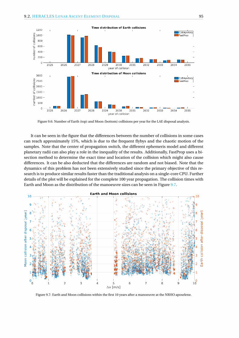
9.2. HERACLES LUNAR ASCENT ELEMENT DISPOSAL 95
Figure 9.6: Number of Earth (top) and Moon (bottom) collisions per year for the LAE disposal analysis.
It can be seen in the figure that the differences between the number of collisions in some casescan reach approximately 15%, which is due to the frequent flybys and the chaotic motion of thesamples. Note that the center of propagation switch, the different ephemeris model and differentplanetary radii can also play a role in the inequality of the results. Additionally, FastProp uses a bi-section method to determine the exact time and location of the collision which might also causedifferences. It can be also deducted that the differences are random and not biased. Note that thedynamics of this problem has not been extensively studied since the primary objective of this re-search is to produce similar results faster than the traditional analysis on a single-core CPU. Furtherdetails of the plot will be explained for the complete 100 year propagation. The collision times withEarth and Moon as the distribution of the manoeuvre sizes can be seen in Figure 9.7.
Figure 9.7: Earth and Moon collisions within the first 10 years after a manoeuvre at the NRHO aposelene.

96 9. STUDY CASES
It can be seen in the figure that there are narrower and wider gaps where no collisions occur, thelargest of them between 3.8 and 5 m/s. Therefore, for this specific departure date, a value betweenthis region should be selected which also leaves margins for manoeuvre errors. Note that for a moredetailed study, an error in the direction of the manoeuvre should be also taken into account. To beable to see the complete behaviour of the dynamics of this problem, the propagation was repeatedfor a period of 100 years. Further conclusions will be drawn based on the longer propagation. Thecollision times with Earth and Moon for the 100-year case can be seen in Figure 9.8.
Figure 9.8: Earth and Moon collisions within the first 100 years after a manoeuvre at the NRHO aposelene.
The figure shows that the gaps disappear as the propagation time is increased, which are causedby long-term resonances with Earth as well as the accumulation of integration errors. Note that theexact location and width of the gaps are highly dependent on the departure date, due to the locationof the Sun. An analytical study of the Bicircular Restricted 4-Body Problem (BCR4BP) showed thatthree possible outcomes exist after applying the manoeuvre: a heliocentric escape directly after de-parture, or after making several revolutions in the Earth-Moon system, and a capture or collision inthe Earth-Moon system [46]. Note that [46] only considered 15 years of propagation after departureof the spacecraft.
It can be seen in Figure 9.8 that the number of collisions within the first 10 years after the ma-noeuvre is much larger than for the rest of the propagation. At later times, the distribution of thecollisions is rather uniform and mainly occurs with Earth. 30-35 years after departure, there is alarger group of Earth collisions at the 4.7-9 m/s manoeuvre, which could be caused by resonant or-bits with Earth. It can also be seen that the number of Earth collisions after 10 years is much greaterthan the number of Moon collisions. This is caused by the fact that the majority of those samplesmade a heliocentric escape, and hitting Earth coming from a heliocentric orbit is much more prob-able than hitting the Moon, because perfect alignment of the Moon is required to be able to collidewith it. The time distribution of the impacts can be seen in Figure 9.9.
This figure shows that most of the Moon collisions occur within the first 5 years of the propaga-tion as was already presented in Figure 9.6. Within this 5-year period, the majority of the collisionshappen in the first year, which is in accordance with the findings in [46]. Within the first 10 yearsafter the manoeuvre, almost twice as many Moon collisions occur than Earth collisions, however be-tween the 10 and 100 year period, more than 10 times more Earth collisions take place than Moon
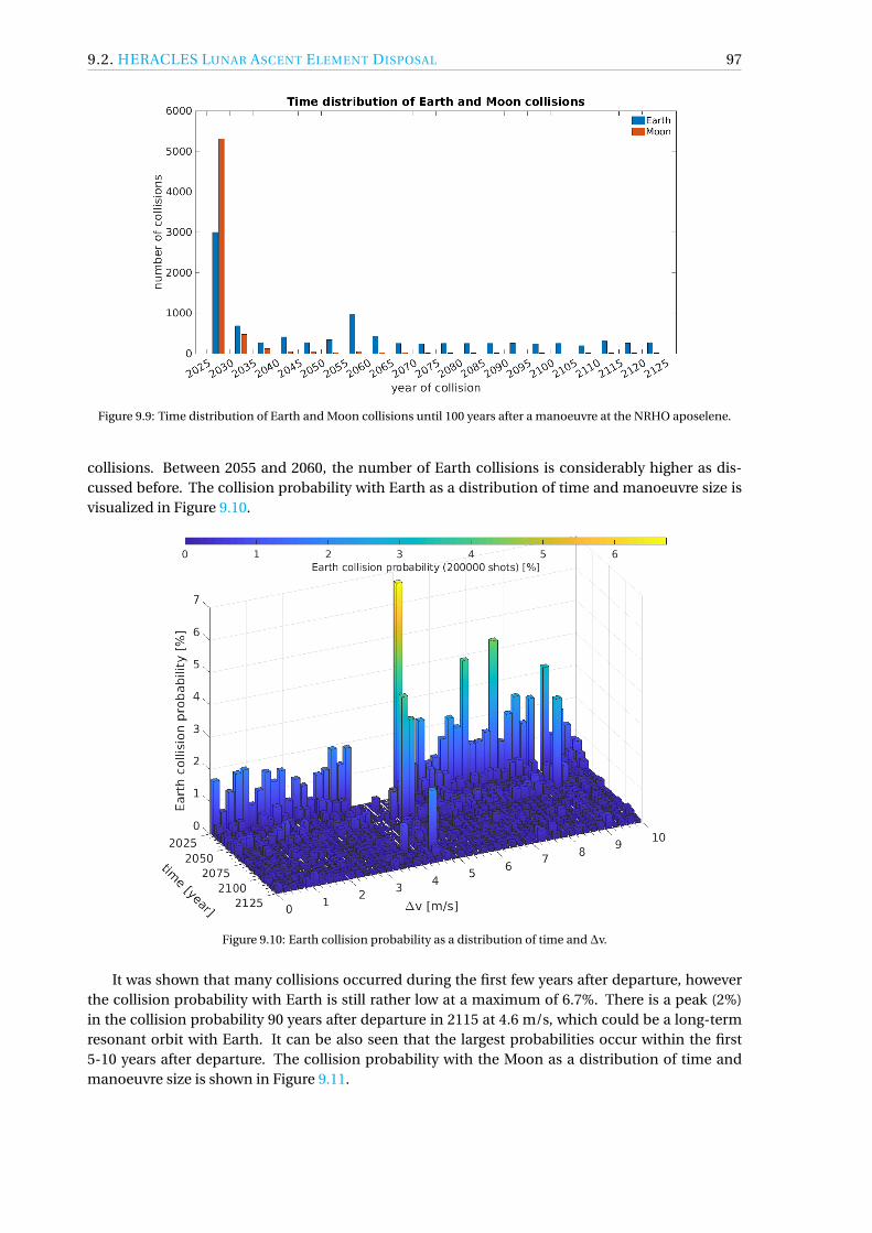
9.2. HERACLES LUNAR ASCENT ELEMENT DISPOSAL 97
Figure 9.9: Time distribution of Earth and Moon collisions until 100 years after a manoeuvre at the NRHO aposelene.
collisions. Between 2055 and 2060, the number of Earth collisions is considerably higher as dis-cussed before. The collision probability with Earth as a distribution of time and manoeuvre size isvisualized in Figure 9.10.
Figure 9.10: Earth collision probability as a distribution of time and ∆v.
It was shown that many collisions occurred during the first few years after departure, howeverthe collision probability with Earth is still rather low at a maximum of 6.7%. There is a peak (2%)in the collision probability 90 years after departure in 2115 at 4.6 m/s, which could be a long-termresonant orbit with Earth. It can be also seen that the largest probabilities occur within the first5-10 years after departure. The collision probability with the Moon as a distribution of time andmanoeuvre size is shown in Figure 9.11.

98 9. STUDY CASES
Figure 9.11: Moon collision probability as a distribution of time and ∆v.
It can be seen that the largest probability of a Moon collision, which is 11%, occurs at 7.4 m/s. Itis presented in the figure that the gaps where zero collisions happen are not closing unlike in Earth’scase. The collision probability after the first 5-10 years is negligible for most manoeuvre sizes exceptfor 9.5-10 m/s, where a considerable amount of collisions occur 15-20 years after the departure fromthe gateway.
To conclude, it was shown for this particular departure date that a manoeuvre between 4 and 5m/s should be selected to avoid high collision probability. To strengthen this assumption, a Monte–Carlo type analysis should to be carried out with larger number of samples within this region toprove that the number of collisions is indeed minimal, however this analysis was not done in thisthesis project. For different departure dates, the same analysis has to be repeated to detect the gapswhere the collision probability is minimal.
After the validation and analysis of the results of CUDAjectory and FastProp, the runtimes of thesimulations are compared. As mentioned before, the simulation using FastProp was only done until10 years after departure. FastProp was executed using a single-core CPU on a local PC at ESOC andon the servers of ESOC using the Parallel Computing Toolbox of MATLAB with 24 threads. Note thatthe output handling is also included in the total runtimes which are tabulated in Table 9.3.
Table 9.3: Total simulation runtimes of the LAE disposal for 200000 samples simulating 10 years using different setups.
Software System CPU GPU Runtime [s]FastProp ESOC Intel Core i7-4790 v3 N/A 33850 (1 core)FastProp ESOC Intel Xeon E5-2690 v3 N/A 2400 (24 cores)
CUDAjectory ESOC Intel Core i7-4790 N/A 3258 (1 core)CUDAjectory ESOC Intel Core i7-4790 GeForce GT630 2095CUDAjectory Argon Intel Xeon Silver 4116 Quadro GP100 235CUDAjectory Argon Intel Xeon Silver 4116 Tesla P100 244CUDAjectory Argon Intel Xeon Gold 5120 GeForce GTX 1080 Ti 227

9.3. ATHENA MIRROR COVER DISPOSAL 99
It can be seen that the simulation times of CUDAjectory run on the different GPUs are showingmuch better performance than FastProp. Even the low-end gaming GPU (GeForce GT630) seemedto be faster than the parallel version of FastProp. Note that the high-end gaming card (GeForce GTX1080 Ti) produced the best results, which is again due to the large output handling times. The totalspeedup of the best GPU version and the single-core CPU version of CUDAjectory is approximately14. The total runtimes and the integration times of the 100-year propagation run by CUDAjectorycan be seen in Table 9.4.
Table 9.4: Simulation and integration runtimes of the LAE disposal for 200000 samples simulating 100 years.
System CPU GPUTotal
runtime [s]Integration
time [s]Argon Intel Xeon Silver 4116 Quadro GP100 1113 683Argon Intel Xeon Silver 4116 Tesla P100 1195 751Argon Intel Xeon Gold 5120 GeForce GTX 1080 Ti 1063 761
It can be seen that the fastest total simulation was done by the gaming card (GeForce GTX 1080Ti), however the Quadro GP100 outperforms the other cards with its much faster integration times.The integration time of the GeForce GTX 1080 Ti is also really close to the integration time of thecomputing accelerator Tesla P100. Considering these runtimes, it can be concluded that this analy-sis can be done at a fraction of time compared to the simulation times of FastProp.
9.3. ATHENA MIRROR COVER DISPOSALThe Advanced Telescope for High ENergy Astrophysics (ATHENA) mission will be an X-ray telescopedesigned by ESA, which is planned to be launched in 2031. The primary goals of the mission will beto map hot gas structures and determine their physical properties as well as to search for supermas-sive black holes. Its final orbit will be a halo orbit around the L2 Lagrange point of the Sun-Earthsystem. The telescope will have an effective area of approximately 2 m2 and a focal length of 12 m.The spacecraft will contain two instruments, the X-ray Integral Field Unit for high-spectral resolu-tion imaging, and the Wide Field Imager for high count rate, moderate resolution spectroscopy [47].
The spacecraft will be launched by the Ariane 6 launcher and it will reach its operational orbitwith a direct transfer trajectory. The spacecraft contains a large mirror cover to protect the tele-scope throughout the launch, which will be released into a heliocentric orbit during the transfer toL2. However, the release of this object has to comply with space debris mitigation requirements,therefore a disposal study needs to be carried out [41].
The transfer trajectory to L2 contains multiple Trajectory Correction Maneuvers (TCMs). Themirror cover will be released after executing the second TCM, which will be deliberately larger thanthe optimal manoeuvre in order to release the mirror cover into a heliocentric orbit since the L2transfer orbit is considered as Earth-centric. The analysis by CUDAjectory will be compared to theresults of SNAPPshot.
The input data for the disposal analysis contained the state of the spacecraft after the secondTCM, varying the additional∆v that is accounted to make a heliocentric escape. The size of the ma-noeuvre was varied between 0.1 and 10 m/s in 0.01 m/s steps, which made 991 batches in total. Eachbatch contained 1000 samples, therefore the total number of samples in this simulation was 991000.The manoeuvres in each batch are perturbed by size using a -1.0-0.1 m/s uniform distribution andperturbed by direction using a 0-3.5 uniform distribution for the half cone angle. This perturbationwas intended to make a more realistic situation to reproduce the imperfections of the manoeuvres.The center of propagation for both software was the Sun. The dynamical model used in this simula-tion was the third-body perturbation by all the planets, Pluto and the Moon. The simulation periodwas fixed to 100 years, and 10−8 was used as an integration tolerance.

100 9. STUDY CASES
The study investigated the return probability of the mirror cover to Earth’s vicinity which wasset to be 500000 km in radius. Note that this value is approximately half the size of the SOI of Earth.Since the initial positions of the samples are beyond this 500000 km limit, collision checks wereenabled with a collision radius increased to this value, therefore the SOI crossing check did not haveto be enabled.
The study was repeated using the same initial conditions with SRP as an additional perturbingforce and a varying area-to-mass ratio between 0 and 0.1 m2/kg using a uniform distribution tomodel the tumbling of the mirror cover. The goal was to see the effect of SRP on the statistics,and find regions in ∆v where both simulations show low probability Earth returns. The differencesbetween the SNAPPshot and CUDAjectory results for the return probability are shown in Figure 9.12.
Figure 9.12: Differences between the return probabilities of the ATHENA mirror cover without (top) and with SRP (bot-tom) produced by SNAPPshot and CUDAjectory.
It can be seen in the figure that the differences are rather small and extremely noisy, thereforethey do not show systematic errors for both cases. The peaks at 3, 5.4, and 6 m/s for the case withoutSRP, and at 6 m/s for the case with SRP are caused by the very rapid change in the return probabilitywhich will be shown in Figure 9.13. Considering these small differences the results of SNAPPshotand CUDAjectory can be accepted as statistically equivalent. The return probabilities for differentmanoeuvre sizes for the cases with and without SRP can be seen in Figure 9.13.
Several different regions can be distinguished in the figure. The aim of this investigation is tofind a larger ∆v region where both curves overlap with a fairly low return probability. This region inthis case is in approximately 7.8-8.2 m/s. It can be seen that in case where no SRP was applied thechanges in return probability are much sharper than in the other case. Additional studies showedthat by increasing the area-to-mass ratio, the curve is shifted towards lower manoeuvre sizes witha similar pattern. However, since the effect of SRP highly depends on the position of the Sun, bychoosing another departure date, it is possible that this shift is going to the opposite direction. Itcan be seen that by varying the area-to-mass ratio the results are blurred and the peaks are widerthan in the case without SRP as well as shifted to the left because of the reasons discussed before.
It can be seen that for both cases there is a small region around 5.6-5.8 m/s where all the samplesreturn. Further investigation showed that these orbits are close to a 12:11 resonance with Earth,

9.3. ATHENA MIRROR COVER DISPOSAL 101
Figure 9.13: Return probability of the ATHENA mirror cover with and without SRP.
therefore manoeuvre sizes in this region should be avoided. The time distribution of the returnprobabilities with varying manoeuvres for the case without SRP and for the case with SRP are shownin Figure 9.14 and 9.15 respectively.
Figure 9.14: Earth return probability for the case without SRP as a distribution of time and ∆v.
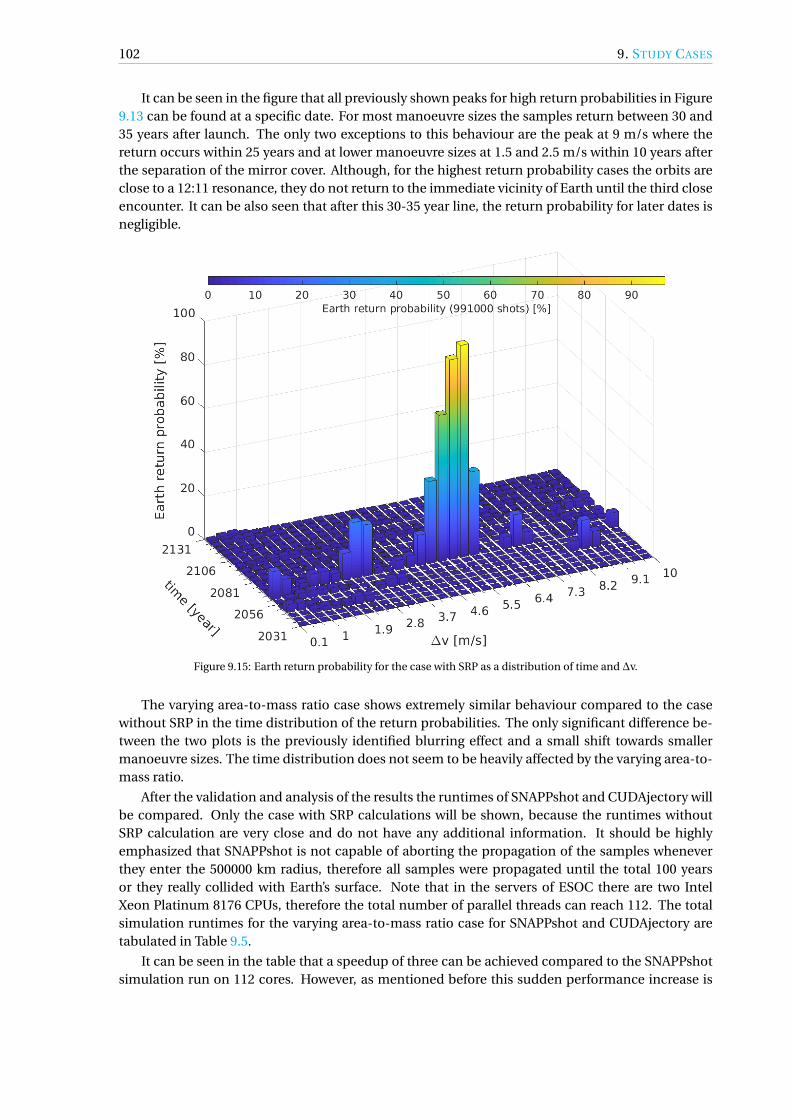
102 9. STUDY CASES
It can be seen in the figure that all previously shown peaks for high return probabilities in Figure9.13 can be found at a specific date. For most manoeuvre sizes the samples return between 30 and35 years after launch. The only two exceptions to this behaviour are the peak at 9 m/s where thereturn occurs within 25 years and at lower manoeuvre sizes at 1.5 and 2.5 m/s within 10 years afterthe separation of the mirror cover. Although, for the highest return probability cases the orbits areclose to a 12:11 resonance, they do not return to the immediate vicinity of Earth until the third closeencounter. It can be also seen that after this 30-35 year line, the return probability for later dates isnegligible.
Figure 9.15: Earth return probability for the case with SRP as a distribution of time and ∆v.
The varying area-to-mass ratio case shows extremely similar behaviour compared to the casewithout SRP in the time distribution of the return probabilities. The only significant difference be-tween the two plots is the previously identified blurring effect and a small shift towards smallermanoeuvre sizes. The time distribution does not seem to be heavily affected by the varying area-to-mass ratio.
After the validation and analysis of the results the runtimes of SNAPPshot and CUDAjectory willbe compared. Only the case with SRP calculations will be shown, because the runtimes withoutSRP calculation are very close and do not have any additional information. It should be highlyemphasized that SNAPPshot is not capable of aborting the propagation of the samples wheneverthey enter the 500000 km radius, therefore all samples were propagated until the total 100 yearsor they really collided with Earth’s surface. Note that in the servers of ESOC there are two IntelXeon Platinum 8176 CPUs, therefore the total number of parallel threads can reach 112. The totalsimulation runtimes for the varying area-to-mass ratio case for SNAPPshot and CUDAjectory aretabulated in Table 9.5.
It can be seen in the table that a speedup of three can be achieved compared to the SNAPPshotsimulation run on 112 cores. However, as mentioned before this sudden performance increase is
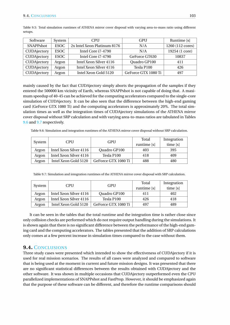
9.4. CONCLUSIONS 103
Table 9.5: Total simulation runtimes of ATHENA mirror cover disposal with varying area-to-mass ratio using differentsetups.
Software System CPU GPU Runtime [s]SNAPPshot ESOC 2x Intel Xeon Platinum 8176 N/A 1260 (112 cores)
CUDAjectory ESOC Intel Core i7-4790 N/A 19254 (1 core)CUDAjectory ESOC Intel Core i7-4790 GeForce GT630 10837CUDAjectory Argon Intel Xeon Silver 4116 Quadro GP100 411CUDAjectory Argon Intel Xeon Silver 4116 Tesla P100 426CUDAjectory Argon Intel Xeon Gold 5120 GeForce GTX 1080 Ti 497
mainly caused by the fact that CUDAjectory simply aborts the propagation of the samples if theyentered the 500000 km vicinity of Earth, whereas SNAPPshot is not capable of doing that. A maxi-mum speedup of 40-45 can be achieved for the computing accelerators compared to the single-coresimulation of CUDAjectory. It can be also seen that the difference between the high-end gamingcard (GeForce GTX 1080 Ti) and the computing accelerators is approximately 20%. The total sim-ulation times as well as the integration times of CUDAjectory simulations of the ATHENA mirrorcover disposal without SRP calculation and with varying area-to-mass ratios are tabulated in Tables9.6 and 9.7 respectively.
Table 9.6: Simulation and integration runtimes of the ATHENA mirror cover disposal without SRP calculation.
System CPU GPUTotal
runtime [s]Integration
time [s]Argon Intel Xeon Silver 4116 Quadro GP100 403 395Argon Intel Xeon Silver 4116 Tesla P100 418 409Argon Intel Xeon Gold 5120 GeForce GTX 1080 Ti 488 480
Table 9.7: Simulation and integration runtimes of the ATHENA mirror cover disposal with SRP calculation.
System CPU GPUTotal
runtime [s]Integration
time [s]Argon Intel Xeon Silver 4116 Quadro GP100 411 402Argon Intel Xeon Silver 4116 Tesla P100 426 418Argon Intel Xeon Gold 5120 GeForce GTX 1080 Ti 497 489
It can be seen in the tables that the total runtime and the integration time is rather close sinceonly collision checks are performed which do not require output handling during the simulations. Itis shown again that there is no significant difference between the performance of the high-end gam-ing card and the computing accelerators. The tables presented that the addition of SRP calculationsonly comes at a few percent increase in simulation times compared to the case without them.
9.4. CONCLUSIONSThree study cases were presented which intended to show the effectiveness of CUDAjectory if it isused for real mission scenarios. The results of all cases were analyzed and compared to softwarethat is being used at the moment in current and future mission designs. It was presented that thereare no significant statistical differences between the results obtained with CUDAjectory and theother software. It was shown in multiple occasions that CUDAjectory outperformed even the CPUparallelized implementations of SNAPPshot and FastProp. However, it should be emphasized againthat the purpose of these software can be different, and therefore the runtime comparisons should

104 9. STUDY CASES
be taken with great care. Nevertheless, it can be concluded that CUDAjectory could be a valid toolin the future for these kind of analysis.
It can be seen in the performance of the different GPUs that for the presented cases, a high-endgaming GPU is only 10-30% slower than the computing accelerator cards. Therefore, it is worth con-sidering to run these simulations on a high-end gaming GPUs in the future considering the factor often price difference compared to a computing accelerator.

10 CONCLUSIONS AND RECOMMENDATIONS
This chapter will conclude the report and discuss some recommendations for future work.
10.1. CONCLUSIONSThe main objective of this thesis research was to study the effective utilization of GPUs in massivelyparallelized trajectory propagations. Different aspects of parallel processing were studied with spe-cial focus on GPU programming in Chapter 2. It was shown that the CUDA programming languageis a great choice for GPU programming, since it is one of the most robust and developer friendly APIsfor this purpose, and it includes many features such as dynamic parallelism support or debuggingtools, which makes it applicable for astrodynamics problems.
A robust tool called CUDAjectory was created which is capable of performing parallel trajectorypropagations on CUDA-capable devices. The capabilities of the software were determined by theneeds of the Mission Analysis Section at ESOC, where the thesis was carried out. Primarily, mod-els and tools needed for planetary protection simulations and disposal analysis were added to thesoftware which were described in detail in Chapter 3 and Chapter 4. After several iterations andan optimization process, the final design and high-level algorithmic model of CUDAjectory werepresented in Chapter 5. The core functionalities of the software were collected in a library calledlibtramp, which makes it easily linkable to other projects.
It was shown in Chapter 6 that calculations in single-precision mode are not sufficiently preciseenough for most of the applications, therefore double-precision was used in further analysis. Allmodules of CUDAjecory were successfully validated by a tool called MASW, which is available atESOC. The time evolution of a randomly selected orbit calculated by CUDAjectory and MASW werecompared. It was determined that the differences are negligible for all cases.
Profiling tools such as the NVIDIA Visual Profiler described in Chapter 2 can help developers toidentify bottlenecks and apply optimization methods to their software. Several optimization tech-niques were applied considering the characteristics of GPUs, which were presented in Chapter 7.
Instruction level optimizations recommended by [37] were implemented at the most commonlyused code segments such as the two-body force evaluation which improved the performance of thesoftware by 1-2%. Static optimization was considered to select the best block size of the kernel tomaximize the performance of the software.
A powerful clustering algorithm was implemented to sort and filter the propagated samples toachieve higher speedups during execution. This algorithm stops the integration after a certain num-ber of integration step attempts (which includes the failed attempts during variable time step inte-gration as well), which is determined by the user, sorts and filters the samples or collects output. Itwas shown that a value between 200 and 400 attempts is optimal for most cases. The performanceimprovement of this algorithm is different on each device and can reach 50% in some scenarios.
Asynchronous output handling was designed into the clustering algorithm which can signifi-cantly decrease the total simulation time by allowing concurrent execution of the integration andoutput handling logic. It was identified that the largest relative time can be saved if the integra-tion and output handling times are comparable, which is the case for low-end gaming GPUs. Theintegration time in simulations run by high-end GPUs is usually much smaller than the output han-dling time, therefore applying the asynchronous algorithm does not change the total runtime sig-nificantly.
It was identified that optimizing the ephemeris retrieval is a crucial part of the simulations toachieve high performance, therefore several techniques were applied to speed up the calculations.Currently available ephemeris libraries, such as SPICE, cannot be used on a GPU, therefore all al-gorithms had to be implemented from scratch. Ephemeris data was placed into texture memory
105

106 10. CONCLUSIONS AND RECOMMENDATIONS
which allowed 10-20% performance increase. The number of ephemeris retrievals per integrationstep was minimized by re-using the already calculated positions in intermediate integration steps.
Two gravity models were implemented in CUDAjectory, the spherical harmonics and point mas-con models. It was shown that for parallel integration, even after optimization (dynamic paral-lelism), the point mascon model is not as efficient as the spherical harmonics model due to thelarge number of memory load instructions during the force model evaluation. The execution timedifference between the two gravity models also heavily depends on the used GPU as the differenceis much larger on scientific accelerators than on gaming GPUs.
The performance of the GPU and single-core CPU versions of CUDAjectory were extensivelytested and compared using many cases in Chapter 8. It was shown that on a GPU there is a sig-nificant increase in the integration time (up to 50%) if different epochs are used for the samplescompared to the case when all samples have the same initial epoch. Speedups of 30-40 can beachieved by using sufficiently large number of samples and applying third-body perturbations ofSolar System bodies as a dynamical model. The highest, up to two orders of magnitude speedupscompared to the CPU version can be achieved by using a high-fidelity spherical harmonics model. Itwas also shown that the performance difference between a high-end gaming GPU and a computingaccelerator GPU is largest when the spherical harmonics model is applied. Orbits from circular tohighly elliptical were propagated at the same time on a GPU with much smaller speedups than theother cases. Idling threads were identified as the cause of this performance drop. If the completetrajectory is stored during simulation, the execution becomes I/O-intensive, therefore the speedupsdecrease again because GPUs are not optimized for extensive I/O operations.
Three study cases were presented to show the efficiency of CUDAjectory when applied to realmission scenarios. The three cases were the upper stage disposal of the BepiColombo launch vehi-cle, the heliocentric disposal of the Lunar Ascent Element of the HERACLES mission, and the dis-posal of the mirror cover of ATHENA. In all three cases the results were analyzed and compared toexisting software which are available at the Mission Analysis Section of ESOC. The performance ofthese software was compared to CUDAjectory. The GPU software proved to be extremely efficientin these calculations and outperformed the parallel versions of the existing software. It was alsopresented that the performance difference between high-end gaming GPUs and computing accel-erator cards is only 10-30%, which is caused by the relatively low throughput the execution is ableto achieve.
10.2. RECOMMENDATIONSThe most important recommendation for future work would be the extension of the capabilitiesof the software. These include the addition of other integrators and force models such as an atmo-spheric model. Currently the software is only capable of integrating Cartesian coordinates, and withthe generalization of the EOM it would be possible to integrate Keplerian or equinoctial elements aswell.
An event-detection algorithm using a root-finding method could be added to refine the exactlocations of eclipses, collisions, etc., however this kind of implementation would break the controlflow of the execution and cause warp divergence which should be avoided on a GPU.
Currently the samples are stored in an AoS pattern, however profiling showed that it is poten-tially better for caching and memory coalescence if they are stored in an SoA style. However, SoA isnot a convenient option for object-oriented design although there might be a sophisticated imple-mentation which retains readability of the code by changing the style of the sample storage.
The number of registers used by the kernel changes the performance of the software signifi-cantly, however this was not tested extensively for different GPUs. Increasing or decreasing theregister count during compilation might change the performance on different devices in anotherway. The number of threads within a block is currently fixed to 128, however it is possible that for

10.2. RECOMMENDATIONS 107
each device there is an even more optimal number. It is highly likely that 128 is not optimal for allapplications and devices.
The optimal size of the so-called break size in the cluster simulator algorithm can be changedfrom case to case and even within simulations similarly to the adaptive step size calculation of theintegration step. Empirical analysis showed that choosing a number between 200 and 400 gives thebest performance of the simulations.
It was shown in Chapter 8 that initial orbits that are similar starting from the same initial epochsare recommended to be able to see higher speedups compared to CPU simulations. Storing thecomplete trajectories of the samples in the current format is not recommended, however with someeven more sophisticated output handling logic, the storage time can be decreased.
The performance difference between high-end gaming GPUs and computing accelerators isonly 20-30% in most cases except if spherical harmonics is included in the calculations. In thatcase the speedup of the computing accelerator cards compared to high-end gaming GPUs can beup to an order of magnitude. However, considering the large price difference between these typesof devices, it is not recommended purchasing a computing accelerator card if simulations usingspherical harmonics calculations are not extensively executed.


A CPU AND GPU SPECIFICATIONS
Table A.1: Specifications of the CPUs used for the simulations (various sources).
System CPU Clock rate Core/Thread L1$ L2$ L3$ESOC Intel Core i7-4790 3.6 GHz 4C/2T 64 kB 256 kB 8 MBESOC Intel Xeon Platinum 8176 2.1 GHz 28C/56T 64 kB 256 kB 38.5 MBESOC Intel Xeon Processor E5-2690 v3 2.6 GHz 12C/24T 64 kB 256 kB 30 MBArgon Intel Xeon Silver 4116 2.1 GHz 12C/2T 64 kB 1024 kB 16 MBArgon Intel Xeon Gold 5120 2.2 GHz 14C/2T 64 kB 1024 kB 19 MB
Laptop Intel Core i7-6820HQ 2.7 GHz 4C/2T 64 kB 256 kB 8 MB
Table A.2: Specifications of the GPUs used for the simulations (various sources).
GPU GeForce GT630 Tesla P100 Quadro GP100 GeForce GTX 1080 Ti GeForce 940MXSystem ESOC Argon Argon Argon Laptop
Architecture Kepler Pascal Pascal Pascal MaxwellChip GK107 GP100 GP100 GP102 GM108M
Compute Capability 3.0 6.0 6.0 6.1 5.0SM 1 56 56 28 3
CUDA cores 192 3584 3584 3584 384Clock rate 876 MHz 1.33 GHz 1.44 GHz 1.58 GHz 1.24 GHz
Global mem. type DDR3 HBM2 HBM2 GDDR5X DDR3Global mem. size 2 GB 16 GB 16 GB 11 GB 2 GB
L1$ size 48 kB 24 kB 24 kB 48 kB 24 kBL2$ size 256 kB 4 MB 4 MB 2.75 MB 1 MB
109

BIBLIOGRAPHY
[1] R. P. Russell and N. Arora, “A GPU Accelerated Multiple Revolution Lambert Solver for FastMission Design,” in AAS/AIAA Astrodynamics Specialist Conference, vol. 136, (Toronto, Ontario,Canada), 2010.
[2] N. Arora, High Performance Algorithms to Improve the Runtime Computation of Spacecraft Tra-jectories. PhD thesis, Georgia Institute of Technology, Aug 2013.
[3] D. Izzo, “PyGMO and PyKEP: Open Source Tools for Massively Parallel Optimization in Astrody-namics - the Case of Interplanetary Trajectory Optimization,” in 5th International Conferenceon Astrodynamics Tools and Techniques (ICATT), (Noordwijk, the Netherlands), 2012.
[4] W. V. Wittig, A. and D. Izzo, “On the use of GPUs for Massively Parallel Optimization of Low-Thrust Trajectories,” in 6th International Conference on Astrodynamics Tools and Techniques(ICATT), (Darmstadt, Germany), 2016.
[5] P. W. Kenneally and H. Schaub, “Parallel Spacecraft Solar Radiation Pressure Modeling Us-ing Ray-Tracing On Graphic Processing Unit,” in 68th International Astronautical Congress,no. IAC-17,C1,4,3,x40634, (Adelaide, Australia), International Astronautical Federation, 2017.
[6] M. K. Kaleem and J. Leitner, “Cuda massively parallel trajectory evolution,” in GPUs for Ge-netic and Evolutionary Computation at the Genetic and Evolutionary Computation Conference(GECCO), (Dublin, Ireland), 2011.
[7] S. Wagner, B. Kaplinger, and B. Wie, “GPU Accelerated Genetic Algorithm for Multiple Gravity-Assist and Impulsive ∆V Maneuvers,” in AIAA/AAS Astrodynamics Specialist Conference, (Min-neapolis, MN, USA), American Institute of Aeronautics and Astronautics, Aug 2012.
[8] F. Biscani, D. Izzo, and C. H. Yam, “A Global Optimisation Toolbox for Massively Parallel Engi-neering Optimisation,” arXiv preprint arXiv:1004.3824, Apr 2010.
[9] L. Nyland, M. Harris, J. Prins, et al., “Fast N-body Simulation with CUDA,” GPU Gems, vol. 3,no. 1, pp. 677–696, 2007.
[10] E. B. Ford, “Parallel algorithm for solving Kepler’s equation on Graphics Processing Units: Ap-plication to analysis of Doppler exoplanet searches,” New Astronomy, vol. 14, no. 4, pp. 406–412, 2009.
[11] V. Vittaldev and R. P. Russell, “Space Object Collision Probability via Monte Carlo on the Graph-ics Processing Unit,” The Journal of the Astronautical Sciences, vol. 64, pp. 285–309, Sep 2017.
[12] K. Liu, B. Jia, G. Chen, K. Pham, and E. Blasch, “A real-time orbit SATellites Uncertainty prop-agation and visualization system using graphics computing unit and multi-threading process-ing,” in IEEE/AIAA 34th Digital Avionics Systems Conference (DASC), (Prague, Czech Republic),pp. 8A2–1–8A2–10, Sep 2015.
[13] M. Massari, P. Di Lizia, and M. Rasotto, “Nonlinear Uncertainty Propagation in AstrodynamicsUsing Differential Algebra and Graphics Processing Units,” Journal of Aerospace InformationSystems, vol. 14, pp. 1–11, Jul 2017.
[14] N. Arora, V. Vittaldev, and R. Russell, “Parallel Computation of Trajectories Using Graphics Pro-cessing Units and Interpolated Gravity Models,” Journal of Guidance, Control, and Dynamics,vol. 38, pp. 1–11, May 2015.
110

BIBLIOGRAPHY 111
[15] J. Cheng, M. Grossman, and T. McKercher, Professional CUDA C Programming. Wrox, 1st ed.,2014.
[16] T. Soyata, GPU Parallel Program Development Using CUDA. Chapman & Hall/CRC Computa-tional Science, Chapman and Hall/CRC, 1st ed., 2018.
[17] J. Sanders and E. Kandrot, CUDA by Example: An Introduction to General-Purpose GPU Pro-gramming. Addison-Wesley, 1st ed., 2010.
[18] NVIDIA, CUDA C Programming Guide, Nov 2017. PG-02829-001_v9.1.
[19] NVIDIA, Profiler User’s Guide, Nov 2017. DU-05981-001_v9.1.
[20] NVIDIA, CUDA-GDB CUDA Debugger, Nov 2017. DU-05227-042_v9.1.
[21] K. F. Wakker, Fundamentals of Astrodynamics. Institutional Repository Delft University of Tech-nology, Jan 2015.
[22] G. Petit and B. Luzum, “IERS Conventions (2010),” Technical Note 36, Verlag des Bundesamtsfür Kartographie und Geodäsie, 2010.
[23] “SPICE Toolkit.” https://naif.jpl.nasa.gov/naif/toolkit.html, 2018. Accessed: 2018-05-15.
[24] O. Montenbruck and E. Gill, Satellite Orbits. Springer Berlin, 2001.
[25] B. A. Archinal, M. F. A’Hearn, E. Bowell, A. Conrad, G. J. Consolmagno, R. Courtin, T. Fukushima,D. Hestroffer, J. L. Hilton, G. A. Krasinsky, et al., “Report of the IAU Working Group on Carto-graphic Coordinates and Rotational Elements: 2009,” Celestial Mechanics and Dynamical As-tronomy, vol. 109, no. 2, pp. 101–135, 2011.
[26] R. P. Russell and N. Arora, “Global Point Mascon Models for Simple, Accurate, and Paral-lel Geopotential Computation,” Journal of Guidance, Control, and Dynamics, vol. 35, no. 5,pp. 1568–1581, 2012.
[27] “Global Mascon Geopotential Model.” https://sites.utexas.edu/russell/publications/code/mascon-geopotential/, 2018. Accessed: 11-10-2018.
[28] J. R. Wertz, Orbit and Constellation Design and Management. Microcosm Press/Springer,2nd ed., 2009.
[29] “JPL Ephemerides.” https://ssd.jpl.nasa.gov/?ephemerides, 2018. Accessed: 2018-05-15.
[30] X. X. Newhall, “Numerical Representation of Planetary Ephemerides,” Celestial Mechanics,vol. 45, pp. 305–310, 1989.
[31] E. Fehlberg, “Classical Fifth-, Sixth-, seventh-, and Eight-Order Runge-Kutta Formulas withStepsize Control,” tech. rep., National Aeronautics and Space Administration, Oct 1968.
[32] “CMake.” https://cmake.org/, 2018. Accessed: 11-10-2018.
[33] “Boost C++ Libraries.” https://www.boost.org/, 2018. Accessed: 11-10-2018.
[34] NVIDIA, CUDA Compiler Driver NVCC, Nov 2017. TRM-06721-001_v9.1.

112 BIBLIOGRAPHY
[35] “Jim Verner’s Refuge for Runge-Kutta Pairs.” http://people.math.sfu.ca/~jverner/,2018. Accessed: 07-11-2018.
[36] C. Foerste, F. Flechtner, R. Stubenvoll, M. Rothacher, J. Kusche, H. Neumayer, R. Biancale, J.-M. Lemoine, F. Barthelmes, S. Bruinsma, R. Koenig, and C. Dahle, “EIGEN-5C - the new Geo-ForschungsZentrum Potsdam / Groupe de Recherche de Geodesie Spatiale combined gravityfield model,” AGU Fall Meeting Abstracts, Nov 2008.
[37] NVIDIA, CUDA C Best Practices Guide, Nov 2017. DG-05603-001_v9.1.
[38] NVIDIA, Thrust Quick Start Guide, Nov 2017. DU-06716-001_v9.1.
[39] Duane Merrill, “CUDA Unbound (CUB).” http://nvlabs.github.com/cub, 2018. Accessed:11-11-2018.
[40] “BepiColombo Overview.” http://www.esa.int/Our_Activities/Space_Science/BepiColombo_overview2, 2018. Accessed: 27-11-2018.
[41] ESA Space Debris Mitigation WG, “ESA Space Debris Mitigation Compliance VerificationGuidelines,” Feb 2015.
[42] F. Letizia, C. Colombo, J. Van den Eynde, R. Armellin, and R. Jehn, “SNAPPshot: Suite for thenumerical analysis of planetary protection,” in Proceedings of the 6th International Conferenceon Astrodynamics Tools and Techniques (ICATT), pp. 14–17, 2016.
[43] “Landing on the Moon and Returning Home: HERACLES.” https://www.esa.int/Our_Activities/Human_Spaceflight/Exploration/Landing_on_the_Moon_and_returning_home_Heracles, 2018. Accessed: 27-11-2018.
[44] J. C. Crusan, R. M. Smith, D. A. Craig, J. M. Caram, J. Guidi, M. Gates, J. M. Krezel, and N. B.Herrmann, “Deep space gateway concept: Extending human presence into cislunar space,” inIEEE Aerospace Conference, (Big Sky, MT, USA), pp. 1–10, Mar 2018.
[45] F. Renk, M. Landgraf, and L. Bucci, “Refined Mission Analysis for HERACLES - a Robotic LunarSurface Sample Return Mission Utilizing Human Infrastructure,” in AAS/AIAA AstrodynamicsSpecialist Conference, (Long Beach, CA, USA), Aug 2018.
[46] K. K. Boudad, D. C. Davis, and K. C. Howell, “Disposal Trajectories from Near Rectilinear HaloOrbits,” in AAS/AIAA Astrodynamics Specialist Conference, (Long Beach, CA, USA), Aug 2018.
[47] “ATHENA.” http://sci.esa.int/athena/, 2018. Accessed: 06-12-2018.