mass gap problem on the yangÐmills existence and
TRANSCRIPT

The Phenomenological Motivation of Axions: A Review
Drew Backhouse
On the Yang–Mills Existence andMass Gap Problem
The essential mathematical background and why wecare about the mass gap
Candidate Number:
Dissertation Submitted in Partial Fulfilment of theRequirements for the Degree of
Master of Mathematical and Theoretical Physics
University of OxfordTrinity 2019
Dissertation Submitted in Partial Fulfilment of the Requirements
for the Degree of Master of Mathematical and Theoretical Physics
University of Oxford
Trinity 2021
1
arX
iv:2
108.
0428
5v1
[he
p-ph
] 9
Aug
202
1

Abstract
Setting aside anthropic arguments, there is no reason for CP symmetry to be obeyedwithin the theory of quantum chromodynamics. However, no such violation of CP symmetryhas ever been observed in a strongly interacting experiment. This is known as the strongCP problem which, in its simplest manifestations, can be quantitatively formulated via acalculation of the pion masses and the neutron electric dipole moment. The former yieldsa larger mass for the neutral pion than its charged counterparts, the latter yields a farlarger result than is experimentally measured, where in both cases the discrepancies areparameterised by the physical quantity θ. The strong CP problem can be solved via theinclusion of a new particle, the axion, which dynamically sets θ to zero, eliminating thesetwo manifestations. Thus, experimental searches for such a particle are an active field ofresearch. This dissertation acts as a review of the aforementioned concepts.
2

Contents
1 Introduction 4
2 The Classical Solution To The Strong CP Problem 5
3 The Quantum Solution To The Strong CP Problem 73.1 Chiral Symmetry . . . . . . . . . . . . . . . . . . . . . . . . . . . . . . . . . 73.2 Anomalous Symmetries . . . . . . . . . . . . . . . . . . . . . . . . . . . . . . 83.3 Spurions . . . . . . . . . . . . . . . . . . . . . . . . . . . . . . . . . . . . . . 93.4 Two Flavour QCD . . . . . . . . . . . . . . . . . . . . . . . . . . . . . . . . 103.5 Chiral Symmetry Breaking . . . . . . . . . . . . . . . . . . . . . . . . . . . . 113.6 Low-Energy QCD . . . . . . . . . . . . . . . . . . . . . . . . . . . . . . . . . 13
3.6.1 Pion Kinetic Term . . . . . . . . . . . . . . . . . . . . . . . . . . . . 133.6.2 Pion Mass Term . . . . . . . . . . . . . . . . . . . . . . . . . . . . . . 153.6.3 Nucleon Terms . . . . . . . . . . . . . . . . . . . . . . . . . . . . . . 183.6.4 Effective Lagrangian . . . . . . . . . . . . . . . . . . . . . . . . . . . 20
3.7 The Neutron eDM . . . . . . . . . . . . . . . . . . . . . . . . . . . . . . . . 213.8 The QCD Axion . . . . . . . . . . . . . . . . . . . . . . . . . . . . . . . . . 243.9 Axion-Like Particles . . . . . . . . . . . . . . . . . . . . . . . . . . . . . . . 25
4 Experimental Searches For Axions 284.1 Axion-Photon Conversion . . . . . . . . . . . . . . . . . . . . . . . . . . . . 284.2 Solar Axion Production . . . . . . . . . . . . . . . . . . . . . . . . . . . . . . 284.3 The Axion Helioscope . . . . . . . . . . . . . . . . . . . . . . . . . . . . . . 284.4 The Rise of the Axion Helioscope . . . . . . . . . . . . . . . . . . . . . . . . 304.5 The Legacy of the CERN Axion Solar Telescope . . . . . . . . . . . . . . . . 314.6 The International Axion Observatory: The Final Frontier . . . . . . . . . . . 324.7 A Summary of Axion Helioscopes . . . . . . . . . . . . . . . . . . . . . . . . 35
5 Epilogue 36
Appendix A Reference formulae 39A.1 Scalar QED Feynman Rules . . . . . . . . . . . . . . . . . . . . . . . . . . . 39A.2 Spinor QED Feynman Rules . . . . . . . . . . . . . . . . . . . . . . . . . . . 39A.3 Gamma Matrix Technology . . . . . . . . . . . . . . . . . . . . . . . . . . . 39
Appendix B Axion-Photon Conversion Probability Derivation 40
3

1 Introduction
The reason I can write this dissertation is because, for some inexplicable reason, there issignificantly more matter present in the universe than antimatter and thus the whole uni-verse does not simply annihilate into photons. The question is, why am I not just a photonpropagating in an empty universe?
In 1957, Lev Landau proposed that CP-symmetry is the true symmetry between matterand antimatter [1]. CP-symmetry is the invariance of a system under two successive trans-formations: Charge conjugation (C) and Parity (P). These successive transformations sendall particles to their antiparticles and perform a coordinate inversion. If CP-symmetry wereobeyed, then equal amounts of matter and antimatter would have been created during thebig bang. For anything to exist at all, these must have been separated into totally non-interacting clusters before the universe dropped below about 500 billion Kelvin, otherwise,the matter and antimatter would have mutually annihilated into photons [2]. However, atthis time the longest distances in causal contact were about 100 km, a billionth the sizeof any independent astronomical clusters or galaxies we observe today. Thus, simply fromcausality, the fact we are here today suggests there is not a perfect symmetry between matterand antimatter, undeniable proof that CP-symmetry is allowed to be broken.
Our current mathematical formulation of quantum chromodynamics (QCD) allows forCP-violating terms to be added to the Lagrangian, a prospect we are now totally comfortablewith. However, we have never experimentally observed CP-violation in QCD. An example ofthis is the magnitude of the neutron electric dipole moment (eDM), which (when includingthe CP-violating terms in the Lagrangian) has an experimental upper limit far smaller thanQCD predicts. This can be solved by setting the parameters of the CP-violating terms tozero; this requirement of ‘fine tuning’ our theory is known as the strong CP problem.
The strong CP problem is considered an unsolved problem in physics. There are manyproposed solutions, one of which is the existence of a new particle called the axion. In thisDissertation, we quantitatively formulate the strong CP problem, explaining how the axionsolves it, before generalising to the more abstract axion-like particle and discussing variousmethods of experimentally probing them.
We will assume knowledge of quantum field theory at the level of a masters course.Appendix A contains some reference formulae which we will make use of. If the reader is insearch of a detailed discussion of the basic concepts, I find the book by Mark Srednicki [3]to be a very good read, however, be warned he uses the mostly positive metric conventionwhereas we shall adopt the more commonly used mostly negative metric convention (g =(+−−−)). The book by Michael E. Peskin and Daniel V. Schroder [4] is another standardtext and has a very nice appendix containing all the tools you could ever need (and uses ourmetric convention).
4
2 The Classical Solution To The Strong CP Problem
The existence of a CP-violating strong interaction would result in a predicted neutron elec-tric dipole moment (eDM) of dn ∼ 10−16e cm, while the current experimental upper boundis roughly one-billionth the size [5]. Thus, in one of its simplest manifestations, the strongCP problem is the dilemma that the neutron eDM is measured to be far smaller than wecalculate it to be.
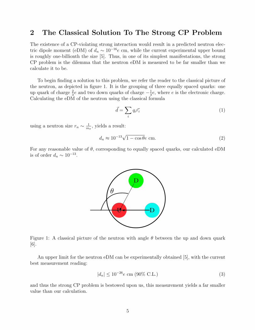
To begin finding a solution to this problem, we refer the reader to the classical picture ofthe neutron, as depicted in figure 1. It is the grouping of three equally spaced quarks: oneup quark of charge 2
3e and two down quarks of charge −1
3e, where e is the electronic charge.
Calculating the eDM of the neutron using the classical formula
~d =∑
i
qi~ri (1)
using a neutron size rn ∼ 1mπ
, yields a result:
dn ≈ 10−13√
1− cos θe cm. (2)
For any reasonable value of θ, corresponding to equally spaced quarks, our calculated eDMis of order dn ∼ 10−13.
U
D
D
2
+2
3� 1
3p = qd (32)
✓ (33)
(34)
FIG. 1: A classical picture of the neutron. From this picture, an estimate of the neutron eDM may be made.
II. THE STRONG CP PROBLEM AND ITS SOLUTIONS AT THE CLASSICAL LEVEL
A. The Strong CP problem
At its heart, the Strong CP problem is a question of why the neutron electric dipole moment (eDM) is sosmall. It turns out that both the problem and all of the common solutions can be described at the classical level.Classically, the neutron can be thought of as composed of a single charge 2/3 up quark and two charge �1/3 downquarks. Asking a student to draw the neutron usually ends up with something similar to that in Fig. 2. If asked tocalculate the eDM of the neutron, the student would simply take the classical formula
~d =X
q~r. (1)
Using the fact that the neutron has a size rn ⇠ 1/m⇡, the student would then arrive at the classical estimate that
|dn| ⇡ 10�13p
1 � cos ✓ e cm (2)
Thus we have the natural expectation that the neutron eDM should be of order 10�13e cm. Because eDMs are avector, they need to point in some direction. The neutron has only a single vector which breaks Lorentz symmetry,and that is its spin. Thus the eDM will point in the same direction as the spin (possibly with a minus sign).
Many experiments have attempted to measure the neutron eDM and the simplest conceptual way to do so isvia a precession experiment. Imagine that an unspecified experimentalist has prepared a bunch of spin up neutronsall pointing in the same direction. The experimentalist then applies a set of parallel electric and magnetic fields tothe system, which causes Larmor precession at a rate of
⌫± = 2|µB ± dE|. (3)
After some time t, the experimentalist turns o↵ the electric and magnetic fields and measures how many of theneutrons have precessed into the spin-down position. This determines the precession frequency ⌫+. The experimen-talist then redoes the experiment with anti-parallel electric and magnetic fields. This new experiment determinesthe precession frequency ⌫�. By taking the di↵erence of these two frequencies, the neutron eDM can be bounded.The current best measurement of the neutron eDM is [1–3]
|dn| 10�26e cm. (4)
We have thus arrived at the Strong CP problem, or why is the angle ✓ 10�13? Phrased another way, the StrongCP problem is simply the statement that the studnet should have drawn all of the quarks on the same line!
3
Figure 1: A classical picture of the neutron with angle θ between the up and down quark[6].
An upper limit for the neutron eDM can be experimentally obtained [5], with the currentbest measurement reading:
|dn| ≤ 10−26e cm (90% C.L.) (3)
and thus the strong CP problem is bestowed upon us, this measurement yields a far smallervalue than our calculation.
5
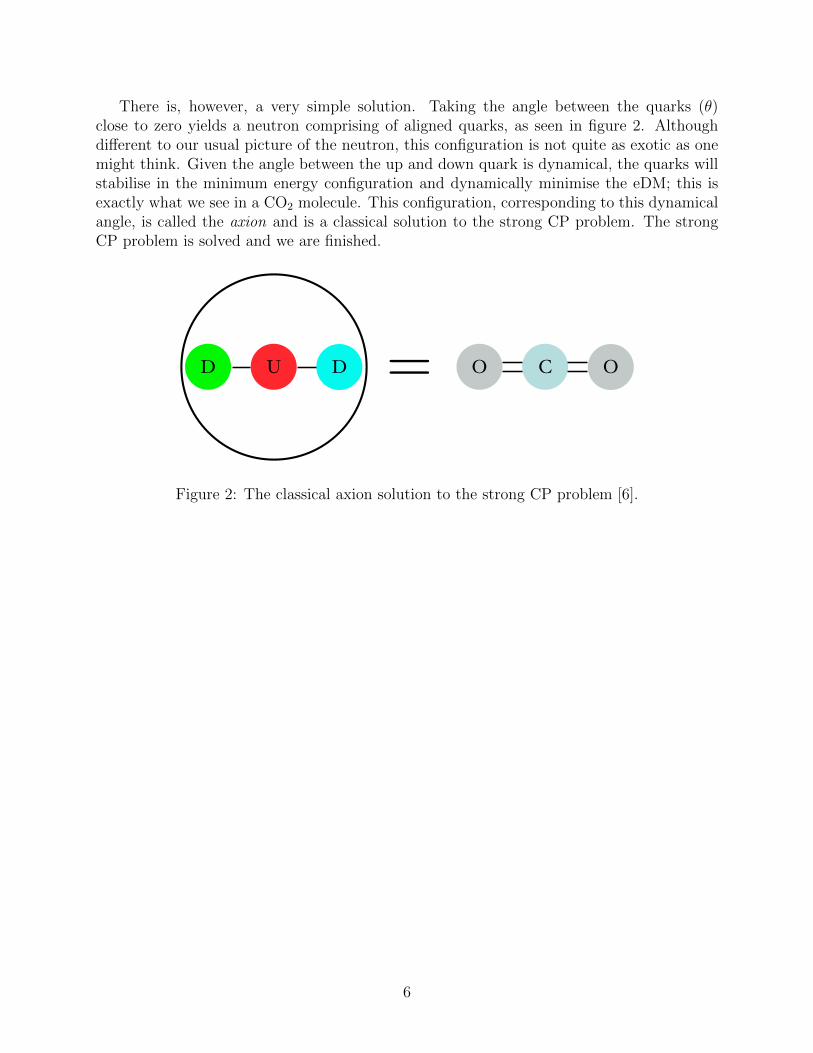
There is, however, a very simple solution. Taking the angle between the quarks (θ)close to zero yields a neutron comprising of aligned quarks, as seen in figure 2. Althoughdifferent to our usual picture of the neutron, this configuration is not quite as exotic as onemight think. Given the angle between the up and down quark is dynamical, the quarks willstabilise in the minimum energy configuration and dynamically minimise the eDM; this isexactly what we see in a CO2 molecule. This configuration, corresponding to this dynamicalangle, is called the axion and is a classical solution to the strong CP problem. The strongCP problem is solved and we are finished.
UD D = CO O
FIG. 2: A axion solution to the Strong CP problem is treating the neutron like CO2. If the angle between the up and downquarks is dynamical, it will relax itself to the minimum energy configuration that has no dipole moment. This dynamicalangle is called the axion.
B. Solutions
There are three solutions to the Strong CP problem that can be described at the classical level. The first requiresthat parity be a good symmetry of nature. Under parity, space goes to minus itself.
P : ~x ! �~x. (5)
We first consider a neutron whose spin and eDM point in the same direction, s = dn. Remembering that angularmomentum is ~s = ~r ⇥ ~p, we have under parity,
P : d ! �d, s ! s. (6)
Thus a neutron is taken from s = dn to s = �dn under parity. We have studied the neutron and it is an experimentalfact that there is only a single neutron whose spin is 1/2. Thus the only option is for the neutron to go to itself under
parity. The only way for both s = dn and s = �dn to be true is if the dipole moment is zero. This is the paritysolution to the Strong CP problem. However, experimentally we have observed that parity is maximally brokenby the weak interactions. Thus it is a bad symmetry of nature and any application to the Strong CP problem isnecessarily more complicated.
The second classical solution is time-reversal (T) symmetry, typically called charge parity (CP) symmetry dueto the fact that the combined CPT symmetry is a good symmetry of nature. Under time reversal,
T : t ! �t. (7)
Considering again a neutron whose spin and eDM point in the same direction, s = dn, we find that under timereversal,
T : d ! d, s ! �s. (8)
As before, a neutron is taken from s = dn to s = �dn. By the same reasoning, this again means that the neutroneDM must be zero. As with parity, CP or equivalently T is not a symmetry of nature and is in fact maximally brokensince the CP-violating phase in the CKM matrix is about ⇡/3.
The last solution that can be seen at the classical level is the axion solution. The situation of having two negativecharges on opposite sides of a positive charge seems very natural, just look at CO2. The plus charged carbon isexactly between the two oxygens with the equilibrium condition being that the angle between the two bonds isexactly ⇡ or in terms of the angle ✓ = 0. The critical idea for making this situation work is that the angle betweenthe two bonds is dynamical. If the initial angle is not ✓ = 0, it quickly relaxes to 0. Motivated by this example, theaxion solution is the idea that the angle ✓ is dynamical and can change. It can be proven that the minimum willalways be at ✓ = 0 [4] and the Strong CP problem is solved.
III. THE STRONG CP PROBLEM AT THE QUANTUM LEVEL
We now formulate the Strong CP problem at the quantum level. As the Strong CP problem is a question aboutthe properties of the neutron, we need to develop a theory of neutrons and low-energy QCD. In this section, we
4
Figure 2: The classical axion solution to the strong CP problem [6].
6
3 The Quantum Solution To The Strong CP Problem
Unfortunately, we have not got off that easy, for there is more to our world than classicalphysics. We must formulate and solve the strong CP problem at the quantum level.
3.1 Chiral Symmetry
Consider an SU(3) gauge theory with one flavour of massless quark. The quark is representedby the Dirac fermion field in the fundamental representation of the gauge group SU(3):
ψ =
(ψL
ψR
)(4)
where ψL and ψR are left- and right-handed Weyl fields, two-component spinors. The vectorgauge boson is called the gluon and is the quanta of the gauge field Aµ.
The classical QCD Lagrangian for one flavour of massless quark reads:
L = iψ /Dψ − 1
4F µν,aF a
µν −g2θ
32π2F µν,aF a
µν (5)
where F aµν = ∂µA
aν−∂νAaµ+gfabcAbµA
cν is the SU(3) valued field strength tensor for the strong
interaction, F µν,a = 12εµνρσF a
ρσ is it’s Hodge dual, and /D := γµ(∂µ − igAµ) is the covariantderivative contracted with the usual gamma matrices. We have also introduced the strongcoupling constant g and an arbitrary parameter θ which parameterises a CP violating term.In case the reader is more familiar with seeing the gauge fields inside a trace, we note the twonotations can be easily moved between by expanding the gauge fields in terms of generatormatrices:
Tr[F µνFµν ] = Tr[F µν,aT aF bµνT
b] = F µν,aF bµνTr[T aT b] = F µν,aF b
µνT (N)δab =1
2F µν,aF a
µν (6)
where we have substituted the Index Tr(T aRT
bR
)= T (R)δab for some representation R and
used that in the fundamental representation T (N) = 12.
In addition to the SU(3) gauge symmetry, this classical Lagrangian has a global symmetry
G = U(1)V × U(1)A (7)
where U(1)V is a vector U(1) symmetry, and U(1)A is an axial U(1) symmetry.
The ‘vector’ and ‘axial’ distinction on these last two global symmetries might be lessfamiliar to the reader, to help explain their origin, consider the Lagrangian (5) in two-component form:
L = iψ†LσµDµψL + iψ†RσµD
µψR −1
4F µν,aF a
µν −g2θ
32π2F µν,aF a
µν (8)
7
where σ := (12, σi) and σ := (12,−σi) with the Pauli spin matrices σi; these act as the
2-component equivalent of the gamma matrices. The Lagrangian can thus possess two typesof global U(1) symmetry:
U(1)V : ψL → eiαψL, ψR → eiαψR ≡ ψ → eiαψ
U(1)A : ψL → e−iαψL, ψR → eiαψR ≡ ψ → eiαγ5
ψ(9)
recalling the chirality operator γ5ψL = −ψL, γ5ψR = ψR. The former is called a vectorU(1) symmetry because the associated Noether current JµV (x) ≡ ψγµψ(x) transforms as avector. The latter is called an axial U(1) symmetry because the associated Noether currentJµA(x) ≡ ψγµγ5ψ(x) transforms as an axial vector (the spacial part is odd under parity).The U(1)A symmetry treats left- and right-handed Weyl fields differently and is thus knownas a chiral symmetry. Note the U(1)A transformation law for ψ:
U(1)A : ψ = ψ†γ0 →(eiαγ
5
ψ)†γ0 = ψ†e−iα(γ5)†γ0 = ψ†γ0eiαγ
5
= ψeiαγ5
(10)
is the same as the U(1)A transformation law for ψ, recalling that (γ5)† = γ5 and {γ5, γµ}=0.The remaining conjugate transformations are obvious (just flip the sign on the i).
3.2 Anomalous Symmetries
We now consider how these symmetries behave upon adding a mass term for the quark andquantising the theory. We start by constructing a mass term for the quark, which must bereal, Lorentz invariant, and gauge invariant. Lorentz and gauge invariance are only satisfiedif we pair up left- and right-handed Weyl spinors, leading us to write down a mass term
LMass?= −mψ†LψR. (11)
However, the fermion masses and the components of the Weyl spinors are in general complex-valued, so to obtain a real, Lorentz invariant, and gauge invariant mass term we must write(11) along with its complex conjugate, yielding a quark mass term
LMass = −mψ†LψR −m∗ψ†RψL. (12)
Explicitly pulling out the arbitrary complex phase of the mass:
m = |m|eiθq (13)
allows us to write (12) in terms of Dirac fields:
Lmass = −|m|ψeiθqγ5ψ. (14)
We observe that applying a U(1)A transformation
U(1)A : −|m|ψeiθqγ5ψ → −|m|ψei(θq+2α)γ5ψ (15)
does not leave the mass term invariant. We thus discover that U(1)A is only an approximatesymmetry of the classical theory which becomes an exact symmetry in the limit of massless
8
quarks.
To quantise this theory, we make use of the path integral:
Z =
∫DADψDψei
∫d4x(iψ /Dψ− 1
4Fµν,aFaµν− g2θ
32π2Fµν,aFaµν) (16)
excluding source terms for brevity. From the Fujikawa method [7], it can be shown that thefunctional measure of the path integral is not invariant under a U(1)A transformation, butrather transforms as
DADψDψ → DADψDψ exp
[i
∫αg2
16π2F µν,aF a
µνdx
](17)
resulting in an additional term in the Lagrangian:
LFuj = αg2
16π2F µν,aF a
µν (18)
and thus a U(1)A transformation does not leave the quantised theory invariant. When agiven symmetry is a good symmetry of the classical theory but not a good symmetry of thequantum theory it is referred to as an anomalous symmetry. Since U(1)A is an approximatesymmetry of the classical theory but not a symmetry at all of the quantised theory, U(1)Ais an anomalous symmetry.
Considering these two effects together, the quantised QCD Lagrangian for one flavour ofmassive quark transforms under the U(1)A transformation as:
LQCD = iψ /Dψ − |m|ψeiθqγ5ψ − 1
4F µν,aF a
µν −g2θ
32π2F µν,aF a
µν
→ iψ /Dψ − |m|ψei(θq+2α)γ5ψ − 1
4F µν,aF a
µν − (θ − 2α)g2
32π2F µν,aF a
µν
(19)
and is no longer invariant. U(1)A is an anomalous symmetry ; it is no longer a good symmetryof nature. Note that in all cases we still have invariance under a U(1)V transformation andthus it is a good symmetry of nature. We may be tempted to just throw U(1)A away, butthat would be too hasty, there is something we can salvage from this apparent tragedy.
3.3 Spurions
We can promote the constants θq and θ to spacetime dependent, fictions, auxiliary fields; θqand θ are then called spurions. We give them the following U(1)A transformations:
U(1)A : θq → θ − 2α, θ → θ + 2α (20)
which cancels the LFuj term and restores the quark mass term to its original form in theU(1)A transformation of the quantised QCD Lagrangian for one flavour of massive quark(19). We thus find that, when introducing spurions, the U(1)A transformation:
ψ → eiαγ5
ψ, θq → θq − 2α, θ → θ + 2α (21)
9
is a good symmetry of the quantised QCD Lagrangian for one flavour of massive quark.
The spurion fields are fictions, auxiliary fields and thus after all is said and done we mustset the spurious fields equal to the constants θq and θ to get our physical theory. U(1)A itselfwill never be a good symmetry of nature but the above transformation (21), which we willcall a spurious symmetry, is.
A final but important note: any physical quantities can only depend on parameters thatare invariant under any good symmetry of nature, such as the above spurious symmetry (21).Thus, any physical quantity cannot depend on θ or θq alone, but only on the combinationθ + θq; clearly invariant under (21).
3.4 Two Flavour QCD
Recall our objective, investigating the strong CP problem. Since the strong CP problem’ssimplest manifestations are in the mass of the pions and the eDM of the neutron, we needto investigate the quantum theory describing neutrons and pions. Since QCD is a theorydescribing quarks, a low-energy QCD effective field theory (EFT) will describe neutrons(nucleons to be exact) which, as we will discover, interact via pions. We thus consider QCDwith 2 light flavours of quarks. In the previous section we had a single quark represented bythe Dirac field ψ. From now on we have two quarks represented by the Dirac fields u and d:
u =
(uL
uR
)d =
(dL
dR
)(22)
where uL, dL and uR, dR are left- and right-handed Weyl fields, two component spinors. Itwill be helpful to define the Weyl field doublets:
ψL =
(uL
dL
)ψR =
(uR
dR
). (23)
The QCD Lagrangian for one flavour of massive quark (19) is easily extended to the case oftwo flavours of massive quark and reads:
LQCD = iu /Du−muueiθuγ5u+ id /Dd−mdde
iθdγ5
d− 1
4F µν,aF a
µν −g2θ
32π2F µν,aF a
µν (24)
where just as before, the up and down quark each have a complex mass with arbitraryphases θu and θd respectively. Considering the Lagrangian (24) in 2-component form, theDirac kinetic terms read:
LQCD ⊃ iu /Du+ id /Dd = iψ†LσµDµψL + iψ†RσµD
µψR (25)
making use of the Weyl field doublets (23). We thus observe a manifest SU(2)L × SU(2)Rglobal 2-flavour symmetry for the left- and right-handed Weyl field doublets:
SU(2)L : ψL → LψL
SU(2)R : ψR → RψR(26)
10

where L ∈ SU(2)L, R ∈ SU(2)R, and thus L†L = 12, R†R = 12. However, the Dirac massterms read:
LQCD ⊃−muueiθuγ5u−mdde
iθdγ5
d
=−muu†LuR −m∗uu†RuL −mdd
†LdR −m∗dd†RdL
(27)
using complex quark masses for ease of notation. This is clearly not invariant under anSU(2)L × SU(2)R transformation due to the quark masses. For the case of equal quarkmasses (mu = md = m) (27) becomes:
−mψ†LψR −m∗ψ†RψL (28)
which transforms under an SU(2)L × SU(2)R transformation as:
SU(2)L × SU(2)R : −mψ†LψR −m∗ψ†RψL → −mψ†LL†RψR −m∗ψ†RR†LψL. (29)
This is only invariant for the case of L ≡ R, we call this a vector SU(2)L × SU(2)R trans-formation. The case of L 6= R is called an axial SU(2)L×SU(2)R transformation which ourtheory is only invariant under for massless quarks. To aid in our description we can equiva-lently write: SU(2)L × SU(2)R ≡ SU(2)V × SU(2)A where SU(2)V and SU(2)A are vectorand axial SU(2)L×SU(2)R transformations. The SU(2)V and SU(2)A symmetries are thusonly approximate symmetries of our theory which become exact symmetries in the equalquark mass and massless quark limits respectively; the former is known as isospin symme-try. A final note: the differing electromagnetic charge of the quarks also contributes to theapproximate nature of these symmetries; QED breaks SU(2)L × SU(2)R symmetry. Sincewe only consider QCD this will not play an important role, but is mentioned for completeness.
Our theory of QCD for two light flavours of quarks is thus approximately invariant underthe global symmetries SU(2)V × SU(2)A and exactly invariant under the global symmetryU(1)V and the two transformations:
u→ eiαγ5
u, θu → θu − 2α, θ → θ + 2α
d→ eiαγ5
d, θd → θd − 2α, θ → θ + 2α(30)
which are just two copies of the spurious symmetry we found in the previous section (21),one for each quark flavour. θu, θd, and θ are spurions.
3.5 Chiral Symmetry Breaking
It is an experimental observation that the quark condensate has a non-zero vacuum expec-tation value (vev):
〈ψRψ†L〉 = −v312 (31)
and thus the approximate SU(2)L×SU(2)R symmetry is spontaneously broken, as a preferreddirection of the quark doublets is chosen while in the ground state. This process is calledspontaneous symmetry breaking (SSB). A field which is not turned off in the vacuum is totallyunphysical and indeed will not correspond to physical states when the system undergoes SSB.We thus perform a field expansion of the quark condensate around its non-zero vev:
ψRψ†L = −v3U(x) (32)
11

where U(x) is a spacetime dependent unitary matrix, defined as
U(x) := eiπa(x)σa
fπ eiθ (33)
where πa are a set of fields with zero vev (〈πa〉 = 0), σa are a corresponding set of matrices,fπ is a constant with dimensions of mass, and θ is our spurious field which we include sothat the LHS and RHS of (32) transform identically under the spurious symmetry (30), asthey must:
ψRψ†L →ψRψ†Le2iα
−v3U(x)→− v3U(x)e2iα(34)
using the U(1)A transformations of the left- and right-handed Weyl fields (9).
Since the fields πa have zero vev they will describe the physical states of our system afterSSB, the particles we would detect. To determine the number and nature of these particleswe need to investigate the details of the symmetry breaking.
Applying an SU(2)L × SU(2)R transformation to the vev (31) yields:
SU(2)L × SU(2)R : −v312 → −v3(RL†) (35)
using the transformations in (26). Observe that, for the case of L = R, the vev is unchangedunder an SU(2)L×SU(2)R transformation, but if L 6= R, the vev is changed. Thus, SU(2)Ais spontaneously broken but the SU(2)V symmetry remains.
Applying U(1)V and U(1)A transformations to the vev (31) yields:
U(1)V : − v312 → −v3eiα12e
−iα = −v3
U(1)A : − v312 → −v3eiα12e
iα = −v3e2iα(36)
using the transformations for left- and right-handed Weyl fields (9). We observe the vev to beunchanged under a U(1)V transformation but changed under a U(1)A transformation. Thus,the anomalous U(1)A symmetry is spontaneously broken but the U(1)V symmetry remains.
Goldstones therom [8] states:
Whenever a continuous symmetry of the Lagrangian is spontaneously broken, massless ‘Gold-stone bosons’ emerge, with one present for each broken generator of the symmetry.
However, the spontaneously broken symmetry SU(2)A was only ever an approximate sym-metry of our theory. The result of which is that any corresponding Goldstone bosons aris-ing from SSB of this symmetry are not exactly massless, as Goldstone bosons for perfectsymmetries are. We call these almost-massless Goldstone bosons pseudo-Goldstone bosons.Although U(1)A is an approximate symmetry of the classical theory, recall it is not a sym-metry at all of the quantised theory; it is anomalous. Since there is no symmetry at all therewill be no corresponding Goldstone boson after SSB, since there was never a symmetry to
12

break in the first place.
We must now identify the broken generators to find our pseudo-Goldstone bosons. Re-calling that SU(N) has N2−1 generators, the breaking of SU(2)A will have 22−1 = 3 brokengenerators and thus has 3 corresponding pseudo-Goldstone bosons. We thus determine thata = 1, 2, 3 where σa are the Pauli spin matrices and πa are the pseudo-Goldstone bosonsassociated with the breaking of SU(2)A. These are related to the pions:
π0 = π3, π± =1√2
(π1 ± iπ2). (37)
The value of fπ can be determined from the rate of decay of a π+ via the weak interactionand is thus called the pion decay constant with value [9]
fπ ≈ 130 MeV. (38)
We’ve extracted a lot of information about the symmetries of our theory so before pro-ceeding we present a summary of the nature of the symmetries encountered:
• SU(2)V : Approximate symmetry (isospin).
• SU(2)A: Approximate symmetry, spontaneously broken.
• U(1)V : Good symmetry.
• U(1)A: Approximate symmetry, spontaneously broken, anomalous.
Recalling also that the spurious symmetries (30) are good symmetries of our theory.
3.6 Low-Energy QCD
U(x) will act as the effective field of our low-energy QCD EFT. To build the effective La-grangian, we consider all possible terms invariant under the remaining symmetries of ourtheory: SU(2)V × U(1)V and the spurious symmetries (30). Note that since U(1)V actstrivially on U(x) we need not explicitly consider it.
3.6.1 Pion Kinetic Term
We first consider a kinetic term for the pions. A general SU(2)L × SU(2)R transformationof U(x) yields:
SU(2)L × SU(2)R : U(x)→ RU(x)L† (39)
and thus an SU(2)V transformation will act just as (39) but limited to the case of L = R.
Using the cyclicality of the trace and R†L = 12, the simplest term we can think of thatis invariant under an SU(2)V transformation and the spurious symmetries (30) is
L ⊃ Tr[U †U
]. (40)
13
However, since U †U = 12, this term only contributes as an additional constant which canalways be removed from the Lagrangian.
The next term we can think of will involve derivatives and reads:
L ⊃ cTr[∂µU †∂µU
](41)
where c is an arbitrary coefficient. Since the SU(2)V transformation is a global transforma-tion, L and R will commute with the partial derivatives ∂µ and thus (41) is indeed invariant.To get something we can work with on the level of Feynman rules we expand U (33) inpowers of f−1
π :
U =
(12 +
iπaσa
fπ− πaσaπbσb
2f 2π
− iπaσaπbσbπcσc
6f 3π
+ . . .
)eiθ
=
(12 +
iπaσa
fπ− πaπa12
2f 2π
− iπaσaπbπb
6f 3π
+ . . .
)eiθ
(42)
where we have used:
πaσaπbσb =1
2πaπb{σa, σb} =
1
2πaπb2δab = πaπa12 (43)
making use of the pauli spin matrices anti-commutation relation {σa, σb} = 2δab. Substitut-ing the above expansion (42) into (41) and working to leading order in f−1
π :
L ⊃ cTr
[∂µ(12 +
iπaσa
fπ− πaπa12
2f 2π
− iπaσaπbπb
6f 3π
)†∂µ
(12 +
iπcσc
fπ− πcπc12
2f 2π
− iπcσcπdπd
6f 3π
)]
= cTr
[(−i∂
µπaσa
fπ− ∂µπbπb12
f 2π
+ i∂µπaσaπbπb + 2πaσa∂µπbπb
6f 3π
)
×(i∂µπ
cσc
fπ− ∂µπ
cπc12
f 2π
− i∂µπcσcπdπd + 2πcσc∂µπ
dπd
6f 3π
)]
= cTr
[1
f 2π
∂µπa∂µπbσaσb +
1
f 4π
∂µπbπb∂µπ
cπc12 −1
3f 4π
(∂µπaσa)(∂µπcσcπdπd + 2πcσc∂µπ
dπd)
]
= cTr
[1
f 2π
∂µπa∂µπa12 +
1
f 4π
∂µπbπb∂µπ
cπc12 −1
3f 4π
(∂µπa∂µπaπdπd + 2∂µπaπa∂µπ
dπd)12
]
= cTr
[1
f 2π
∂µπa∂µπa12 −
1
3f 4π
(∂µπa∂µπaπdπd − ∂µπaπa∂µπdπd)12
]
=4c
f 2π
(1
2∂µπa∂µπ
a − 1
6f 2π
(∂µπa∂µπaπdπd − ∂µπaπa∂µπdπd)
).
(44)We take c = f 2
π/4 such that the pion kinetic term is in the standard form for a real scalarfield. Thus, to leading order in f−1
π , the pion kinetic term and its naturally arising quarticinteractions read:
L ⊃ 1
2∂µπa∂µπ
a − 1
6f 2π
(∂µπa∂µπaπbπb − ∂µπaπa∂µπbπb). (45)
14

Although there are terms with more derivatives that we could include, these terms will beof O(f−3
π ) and thus (45) gives all possible leading order terms.
The ultraviolet (UV) cut-off for our EFT is Λ ∼ 4πfπ which makes f−1π seem like a
bad expansion parameter. However, it turns out that both tree and 1-loop diagrams yieldapproximately equal contributions when taking (4πfπ)−1 rather than f−1
π ; the former is agood expansion parameter at the energy scales of our EFT and thus we only need to considerleading order terms.
3.6.2 Pion Mass Term
The quark mass terms in our 2 flavour QCD Lagrangian (24) can be written in terms of thequark doublet ψ by the use of a mass matrix M :
L ⊃ −muueiθuγ5u−mdde
iθdγ5
d
= −mueiθuu†LuR −mue
−iθuu†RuL −mdeiθdd†LdR −mde
−iθdd†RdL
= −ψ†LMψR − ψ†RM †ψL
(46)
where the mass matrix M is given by:
M =
(mue
iθu 0
0 mdeiθd
). (47)
We are free to bring this mass matrix into the form
SU(2)V : M →M =
(mu 0
0 md
)ei(θu+θd) (48)
with just one overall phase via an SU(2)V transformation; which our theory is indeed invari-ant under.
Starting with (46) and using the cyclicality of the trace, we can replace the quark con-densate ψRψ
†L with its field expansion (32) and we find:
L ⊃ −ψ†LMψR − ψ†RM †ψL
= −Tr[MψRψ
†L +M †ψLψ
†R
]
= v3Tr[MU +M †U †
]
= −V (U)− V (U)∗
= −2Re [V (U)]
(49)
defining the potentialV (U) := −v3 Tr [MU ] . (50)
The Mass of the pions will thus be given by:
m2πa = 2Re
[∂2V (πa)
∂πa2|πa=〈πa〉
](51)
15
where 〈πa〉 are the vevs of the pions; this is simply the value of the pion fields at the minimumof the potential (49) and can thus be determined by solving
2Re
[∂V (πa)
∂πa|πa=〈πa〉
]= 0. (52)
Substituting the explicit form of the spacetime dependent vev (33) into the potential (50)and expanding to leading order in f−1
π :
V (πa) = −v3Tr
[M
(1 +
iπaσa
fπ− πaσaπbσb
2f 2π
)eiθ]
= −v3Tr
[M
(1 +
iπaσa
fπ− πaπa12
2f 2π
)eiθ] (53)
making use of (43). By substituting (53) into (52) we thus need to solve
2Re
[∂V (πa)
∂πa|πa=〈πa〉
]= −2v3Re
[Tr
[M
(iσa
fπ− 〈π
a〉f 2π
)eiθ]]
= 0. (54)
Observing thatTr [Mσa] = 0 for a = 1, 2 (55)
we thus find〈π1〉 = 〈π2〉 = 0 =⇒ 〈π±〉 = 0. (56)
However, for a = 3:
2Re
[∂V (π3)
∂π3|π3=〈π3〉
]= −2v3Re
[Tr
[M
(iσ3
fπ− 〈π
3〉f 2π
)eiθ]]
= −2v3Re
[Tr
[(i
fπ
(mu 0
0 −md
)− 〈π
3〉f 2π
(mu 0
0 md
))ei(θ+θu+θd)
]]
= −2v3Re
[(i
fπ(mu −md)−
〈π3〉f 2π
(mu +md)
)eiθ]
= 0
(57)where we have defined
θ := θ + θu + θd. (58)
We note the parameter θ is invariant under the spurious symmetries (30) and is thusa candidate for parameterising a physical quantity. Spoiler alert, θ turns out to be thequantum analogue of the classical angle seen in figure 1, which we know experimentally tobe very small; we thus expand the exponential eiθ to leading order in θ. From this we find:
2Re
[∂V (π3)
∂π3|π3=〈π3〉
]= −2v3Re
[(i
fπ(mu −md)−
〈π3〉f 2π
(mu +md)
)(1 + iθ
)]= 0 (59)
16

and from the real part we finally arrive at:
〈π3〉 = 〈π0〉 = θfπmd −mu
mu +md
. (60)
The above vev comprises our first cause for concern. (Pseudo-) Goldstone bosons shouldhave zero vev, yet we find a non-zero vev of the π3 pseudo-Goldstone boson. The vev isparametrised by the arbitrary parameter θ and thus our only way out would be to set this tozero. This seems like a serious problem, requiring a ‘fine tuning’ of our theory. Regardless,we should continue with our calculation of the pion masses.
Armed with these vevs, we can determine the pion masses to leading order in f−1π and θ.
Expanding (50) to leading order in f−1π :
V (πa) = −v3Tr
[M
(1 +
iπaσa
fπ− πaσaπbσb
2f 2π
− iπaσaπbσbπcσc
6f 3π
)eiθ]
= −v3Tr
[M
(1 +
iπaσa
fπ− πaπa
2f 2π
− iπaπaπcσc
6f 3π
)eiθ] (61)
and substituting into (51) yields a mass:
m2πa = −2v3Re
[Tr
[M
(− 1
f 2π
− i〈πa〉σaf 3π
)eiθ]]
= v3Re
[1
f 2π
(mu +md)eiθ + v3 i〈πa〉
f 3π
Tr [Mσa] eiθ].
(62)
Substituting the vevs (56), (60), and expanding to leading order in θ yields:
m2π± = 2v3Re
[1
f 2π
(mu +md)(1 + iθ)
]
=2v3
f 2π
(mu +md)
(63)
and
m2π0 = 2v3Re
[1
f 2π
(mu +md)(1 + iθ)− v3 iθ
f 2π
(mu −md)2
mu +md
(1 + iθ)
]
= 2v3
fπ(mu +md)
[1 + θ2 (mu −md)
2
(mu +md)2
].
(64)
We have found the π0 mass to be dependent on θ. Since θ is invariant under the spu-rious symmetries (30) it is totally okay for it to parameterise a physical quantity such asthe pion mass, however, there is a crippling problem. Turning to our experimentalist friendsit is an observed fact that mπ± ≈ mπ0 , where the lack of equality is due to loop effectsin QED. Our results allow for the mass of the π0 to differ from the mass of the charged
17

pions for a non-zero value of θ, but there is no reason for it to be small. We thus observe thefirst manifestation of the strong CP problem at the quantum level, and it really is a problem.
We shall add the arrow that is this triumph to our quiver and proceed with our pursuitof a full low-energy QCD EFT, so that we may add another with the eDM of the neutron.
3.6.3 Nucleon Terms
We next look at terms involving nucleons. We define the nucleon field as the doublet
N =
(p
n
)(65)
where p = uud is the proton and n = udd is the neutron; all the objects present are Diracfermions. Under a general SU(2)L × SU(2)R transformation, the nucleon field transformsas:
PLN → LPLN
PRN → RPRN(66)
where PL,R := 12(12∓γ5) is a projector picking out either the left- or right-handed part of N .
Using {γµ, γ5} = 0, (γ5)† = γ5, and (γ5)2 = 12, it is easy to verify the following propertiesof PL,R:
PL,Rγ0 ≡ γ0PR,L,
P †L,R ≡ PL,R,
(PL,R)2 ≡ PL,R,
PL,RPR,L ≡ 0.
(67)
An SU(2)V transformation will leave the standard Dirac kinetic term iN /∂N invariant,but not the standard Dirac mass term mNNN . However, an invariant mass term can beconstructed by including appropriate factors of U and U † (33) and reads:
L ⊃ −mNN(U †PL + UPR
)N. (68)
There is one other parity, time-reversal, SU(2)V , and (30) invariant term with only onederivative (recall that we are working to leading order in f−1
π thus only consider terms withone derivative). Including this, we have all the relevant terms involving nucleons:
L ⊃ iN /∂N −mNN(U †PL + UPR
)N − 1
2(λ− 1) iNγµ
(U∂µU
†PL + U †∂µUPR)N (69)
whereλ := −gA
gv= 1.27 (70)
18

is the ratio of axial-vector to vector coupling with its value determined from the decay rateof the neutron via the weak interaction [11].
We can tidy this up a bit by performing a field redefinition of the nucleon field:
N :=(u†PL + uPR
)N (71)
where u2 := U ; equivalently, using u†u = 12, we have:
N =(uPL + u†PR
)N . (72)
Making use of the identities:
∂µU ≡ (∂µu)u+ u (∂µu) ,(∂µu
†)u ≡ −u† (∂µu) ,(73)
and the relations in (67), we can substitute (72) into (69) and ultimately obtain:
L ⊃ iN /∂N −mNNN +N /aN − λN /bγ5N (74)
where we define the hermitian vector fields:
aµ :=1
2i[u† (∂µu) + u
(∂µu
†)] ,
bµ :=1
2i[u† (∂µu)− u
(∂µu
†)] .(75)
One again, expanding u and u† to leading order in f−1π yields:
L ⊃ iN /∂N −mNNN +λ
2fπ∂µπ
aNσaγµγ5N . (76)
As it turns out, the pion-nucleon interaction term is one of the two terms used whencalculating the neutron eDM; it will be helpful to simplify it a bit. Granting it centre stage:
LπNN =λ
2fπ∂µπ
aNσaγµγ5N
= − λ
2fππa∂µ
(Nσaγµγ5N
)
= − λ
2fππa(/∂Nσaγ5N −Nσaγ5/∂N
)
= − λ
2fππa(imNNσaγ5N +Nσaγ5mNN
)
= −igπNNπaNσaγ5N
(77)
19
where we integrate by parts in the second line, anti-commute /∂ and γ5 in the third line,substitute the Dirac equations (i/p − m)N = 0 and (i/p + m)N = 0 in the forth line, anddefine the pion-nucleon coupling constant:
gπNN :=λmN
fπ(78)
in the last line. Note the use of the Dirac equations is only applicable for on-shell nucleons;an approximation we will later see to be justified. Substituting fπ = 130 MeV, λ = 1.27,and mn = 939.6 GeV the pion-nucleon coupling constant takes the value:
gπNN = 9.2. (79)
3.6.4 Effective Lagrangian
The last type of term we could write down will involve all of the above, N ’s, U ’s, and M ’s.There are exactly 3 which are parity, time-reversal, SU(2)V , and (30) invariant with noderivatives that are bilinear in the nucleon field N and have one factor of the quark massmatrix M . Writing them out with arbitrary coefficients:
L ⊃− c1N(MPL +M †PR
)N
− c2N(U †M †U †PL + UMUPR
)N
− c3 Tr(MU +M †U †
)N(U †PL + UPR
)N
− c4 Tr(MU −M †U †
)N(U †PL − UPR
)N.
(80)
Making the same field redefinition (72) takes us to:
L ⊃− 1
2c+N
[uMu+ u†M †u†
]N
+1
2c−N
[uMu− u†M †u†
]γ5N
− c3 Tr[MU +M †U †
]NN
+ c4 Tr[MU −M †U †
]Nγ5N
(81)
where c± := c1 ± c2. As always, we expand the above to leading order in f−1π and θ which
ultimately yields:
L ⊃ −iθµ (c− + 4c4)Nγ5N −θc+µ
fππaNσaN (82)
defining the reduced mass of the quarks:
µ :=mumd
mu +md
(83)
and noting the c3 term vanishes for the case of two light quark flavours. The first termcan be eliminated by making the field redefinition N → e−iαγ
5N which does generatesome extra terms, however, they are not linear in the quark masses and can hence be ne-glected. Thus, only the second term contributes providing a pion-nucleon coupling that
20
violates CP-symmetry. The value of c+ is fixed by the proton neutron mass difference via:c+(mu−md) = mp−mn = −1.3MeV. Using mu = 1.7MeV and md = 3.9MeV yields c+ = 0.6.
We are finally in a position to write down, to leading order, the Lagrangian for a low-energy QCD EFT describing nucleons interacting via pions:
L =1
2∂µπa∂µπ
a − 1
6f 2π
(∂µπa∂µπaπbπb − ∂µπaπa∂µπbπb)
− v3
fπ(mu +md)
[π+π+ + π−π−
]− v3
fπ(mu +md)
[1 + θ2 (mu −md)
2
(mu +md)2
]π0π0
+ iN /∂N −mNNN − igπNNπaNσaγ5N −θc+µ
fππaNσaN .
(84)
3.7 The Neutron eDM
To calculate the eDM of the neutron, we need to evaluate a neutron-photon interaction. Wecan start by adding a term to the effective Lagrangian that represents the neutron eDM.Such a term can easily be written down:
L ⊃ dnFµνnSµνiγ5n (85)
where Sµν := i4[γµ, γν ], F µν := ∂µAν − ∂νAµ is the electromagnetic field strength tensor,
and the coupling constant of the photon-neutron interaction, dn, is the neutron eDM. Thecorresponding Feynman rule is easily read off and we can thus write down the matrix elementfor photon-neutron scattering:
iM = 2dnε∗µ(q)u (p′)Sµνqνiγ5u(p). (86)
We can now recalculate the matrix element for photon-neutron scattering in our low-energy QCD EFT (as developed in §3.6) and equate the two results to determine the neutroneDM. The leading order Feynman diagrams for photon-neutron scattering in our low-energyQCD EFT are shown in figure 3 with the corresponding momentum flow shown in figure4. The reason for their leading order nature is due to an infrared divergence for small loopmomenta since the pions have a low mass in comparison to the other available mass scalesin the theory. This allows us to make the approximation l � p, p′, which will prove usefulwhen calculating the matrix element. Note also that l � p, p′ means the internal proton isnearly on-shell and hence justifies our use of the Dirac equation in the fourth line of (77), aspromised.
We now evaluate the diagrams in figure 3 to calculate the photon-neutron scatteringmatrix element in our low-energy QCD EFT. The two relevant interaction terms from theeffective Lagrangian are:
L ⊃ −igπNNπaNσaγ5N −θc+µ
fππaNσaN . (87)
21

94: Quarks and Theta Vacua 586
π+ π+
γ
n p n
π+ π+
γ
n p n
Figure 94.1: Diagrams contributing to the electric dipole moment of theneutron that are enhanced by a chiral log. The CP violating vertex isdenoted with a cross.
second line of eq. (94.20), and is
LπNN = (gA/fπ)∂µπaN T aγµγ5N , (94.23)
where gA = 1.27. As we did in section 83, we can integrate by parts to putthe derivative on the nucleon fields, and then (for on-shell nucleons) usethe Dirac equation to get
LπNN = −i(gAmN/fπ)πaNσaγ5N . (94.24)
The strongest limit on a CP violating pion-nucleon coupling comes frommeasurements of the electric dipole moment of the neutron. The Feynmandiagrams of fig. (94.1) contribute to an ampitude of the form
T = −2iD(q2)ε∗µ(q)us′(p′)Sµνqνiγ5us(p) , (94.25)
where q = p′ − p. In the q → 0 limit, this corresponds to a term in theeffective lagrangian of
L = D(0)Fµν nSµνiγ5n , (94.26)
where n is the neutron field; see section 64. If the factor of iγ5 was absent,this would represent a contribution of D(0) to the magnetic dipole momentof the neutron. To account for the factor of iγ5, we use
Sµνiγ5 = −12ε
µνρσSρσ (94.27)
to see that eq. (94.26) is equivalent to
L = −D(0)Fµν nSµνn , (94.28)
where Fµν = 12ε
µνρσFρσ is the dual field strength. Since B = −E, eq. (94.26)represents a contribution of D(0) to the electric dipole moment of theneutron dn.
Figure 3: The Feynman diagrams giving the leading-order contribution to the neutron eDM.The CP violating vertex is denoted with a cross [3].
Figure 4: The momentum flow in the diagrams of figure 3 [3].
Substituting the explicit forms for the nucleons (65), the pions (37), and the Pauli spinmatrices yields:
L ⊃ −i√
2gπNN(π+pγ5n+ π−nγ5p
)−√
2θc+µ
fπ
(π+pn+ π−np
)(88)
and we can easily read off the Feynman rules for the CP violating and non-CP violatingpion-nucleon vertices. With these results, along with the reference formulae in appendix A,we can list all the Feynman rules we will require:
• non-CP violating npπ+ vertex:√
2gπNNγ5
• CP violating npπ+ vertex: i√
2θc+µ/fπ
• π+ propagator: ik2−m2
π, k = l ± 1
2q (read off from the first term of (84))
• γπ+π+ vertex: −ie(k1 + k2)µ, k1 = l − 12q, k2 = l + 1
2q (Appendix A.1)
• Nucleon propagator: i /k+mNk2−m2
N, k = l + 1
2(p+ p′) (Appendix A.2)
• Incoming fermion: u(k), k = p (Appendix A.2)
• Outgoing fermion u(k), k = p′ (Appendix A.2)
• Incoming photon: ε∗µ(k), k = q (Appendix A.2)
22

We can now evaluate the Feynman diagrams in figure 3 with the above Feynman rulesto obtain the neutron eDM. The matrix element reads:
iM = −ie√
2gπNN
√2θc+µ
fπε∗µ(q)
×∫ Λ
0
d4l
(2π)4
2lµu (p′)[(−/l − /p+mN
)γ5 + γ5
(−/l − /p+mN
)]u(p)
((l + p)2 −m2N)((l + 1
2q)2 −m2
π
) ((l − 1
2q)2 −m2
π
)(89)
where pµ := 12(p′µ + pµ) and Λ = 4πfπ is the UV cutoff of our EFT. Using {γµ, γ5} = 0, the
numerator greatly simplifies to
u(p′)[(−/l − /p+mN
)γ5 + γ5
(−/l − /p+mN
)]u(p) = 2mN u(p′)γ5u(p). (90)
Using u(p′)γ5u(p) = 0 for p′ = p and noting that q = p′ − p tells us that u(p′)γ5u(p) is zerowhen q is zero and therefore must be linear in q; we can thus set q = 0 everywhere else.Using the aforementioned approximation l � p, p′ we can set (l + p)2 −m2
N = 2p · l in thedenominator. Substituting these simplifications brings our matrix element to
iM = −i4egπNN θc+µmN
fπε∗µ(q)
∫ Λ
0
d4l
(2π)4
(2lµ) u(p′)γ5u(p)
(2p · l) (l2 +m2π)2 . (91)
Any Lorentz vectors lµ will be integrated out, but we must conserve the Lorentz structure.Since p is the only other Lorentz vector present, it must gain the Lorentz index after theintegral is performed. We can thus transfer the Lorentz indices from l to p before integratingand make the replacement:
lµ
p · l =lµp
pνlνp→ lpµ
pνlpν=
pµ
m2N
(92)
further simplifying our matrix element to
iM = −i4eθλc+µ
f 2π
ε∗µ(q)pµu(p′)γ5u(p)
∫ Λ
0
d4l
(2π)4
1
(l2 +m2π)2 . (93)
Making use of the Gordon identity:
pµu(p′)γ5u(p) = u(p′)Sµνqνiγ5u(p) +O(q2)
(94)
verifies that u(p′)γ5u(p) is indeed linear in q and simplifies our matrix element to
iM = −i4eθλc+µ
f 2π
ε∗µ(q)u(p′)Sµνqνiγ5u(p)
∫ Λ
0
d4l
(2π)4
1
(l2 −m2π)2 . (95)
This is now written in terms of a standard integral which evaluates to (i/16π2) ln (Λ2/m2π).
Our matrix element thus has the final form:
iM = eθλc+µ
4π2f 2π
ε∗µ(q)u(p′)Sµνqνiγ5u(p) ln
(Λ2
m2π
). (96)
23
By equating (96) with (86), we can read off the neutron eDM:
dn =eθλc+µ
8π2f 2π
ln
(Λ2
m2π
)(97)
and upon substituting the numerical values of the constants (λ = 1.27, c+ = 0.6, µ = 1.2MeV, Λ = 4πfπ, fπ = 130 MeV, mπ = 135 MeV) gives us a final calculated value of theneutron eDM:
dn = 6.7× 10⁻¹⁷θe cm. (98)
using the conversion eV−1 = 1.97× 10⁻⁷ m.
We once again arrive at a physical quantity parameterised by θ, which is okay since θ isinvariant under the spurious symmetries (30). However, recalling the measured upper boundof the neutron eDM (3), yields a constraint on θ of
θ . 10−10 (99)
and we have once again arrived at the strong CP problem at the quantum level. Recall θis comprised of the coefficient of the CP-violating term in the Lagrangian and the totallyarbitrary phases of the up and down quark masses; there is no good reason for it to be thissmall. This truly is a problem.
3.8 The QCD Axion
One of the simplest solutions to the strong CP problem at the quantum level is what we callthe axion EFT (otherwise known as Peccei–Quinn theory). The EFT consists of a singlenew particle and coupling with an associated Lagrangian:
LPQ =1
2∂µa∂
µa− 1
2m2
aa2 + iu /Du−muue
iθuγ5u+ id /Dd−mddeiθdγ
5
d
− 1
4F µν,aF a
µν −(θ +
a
fa
)g2
32π2F µν,aF a
µν
(100)
where a is the axion field, ma is the mass of its quanta, and f−1a is the axion-gluon coupling.
Along with the addition of the axion kinetic and mass terms, this EFT amounts to makinga replacement in the QCD Lagrangian (24) of
θ → θ +a
fa. (101)
The axion vev, 〈a〉, is thus found from the value of the axion filed at the minimum of thepotential (49) with the replacement (101) applied; we simply need to solve
2Re
[∂VPQ(a)
∂a|a=〈a〉
]= 0 (102)
24
where
VPQ(a) = −v3Tr[Me
iπa(x)σa
fπ ei(θ+afa
)]
= −v3Tr
[(mu 0
0 md
)eiπa(x)σa
fπ
]ei(θ+
afa
)
= −v3Tr
[(mu 0
0 md
)eiπa(x)σa
fπ
](1− i(θ +
a
fa)− (θ +
a
fa)2
)(103)
to leading order in θ. This yields:
2Re
[∂VPQ(a)
∂a|a=〈a〉
]= −2v3Re
[Tr
[(mu 0
0 md
)eiπa(x)σa
fπ
](− i
fa− 2
fa(θ +
〈a〉fa
)
)]= 0
(104)and thus the axion has vev:
〈a〉 = −θfa. (105)
Recall our two offenders, the inconsistency of the π0 mass and the larger than measuredvalue of the neutron eDM. In the axion EFT, they each take the form:
m2π0 = 2
v3
fπ(mu +md)
[1 + (θ +
a
fa)2 (mu −md)
2
(mu +md)2
]
dn = 3.2× 10¹⁶
(θ +
a
fa
)e cm
(106)
by making the replacement (101). When the axion sits in the minimum of its potential(a→ 〈a〉 = −θfa), it dynamically restores the expected mass of the π0 and sets the neutroneDM to zero, solving the strong CP problem in all its manifestations. This is exactly thesame mechanism of dynamically minimising the potential that we saw in the classical axionsolution to the strong CP problem, albeit taking far longer.
We finally made it - the strong CP problem is solved.
3.9 Axion-Like Particles
Now convinced that axions are an elegant solution to the strong CP problem we need todetermine their properties. We start by finding the mass of the axion to leading order inf−1π and θ:
m2a = 2Re
[∂2VPQ(a)
∂a2|a=〈a〉
]
= −2v3Re
[Tr
[(mu 0
0 md
)eiπa(x)σa
fπ
]∂2
∂a2
(1− i(θ +
a
fa)− (θ +
a
fa)2
)|πa=〈πa〉
]
= −2v3Re
[(mu +md)
(− 2
f 2a
)](107)
25
and thus we find the axion-gluon coupling to be directly related to the axion mass:
1
fa=
ma
2v32√mu +md
. (108)
We can eliminate v3 by substituting mπ0 (106):
1
fa=
√2
2mπ0fπma (109)
and inputting the values fπ ≈ 130 MeV and mπ0 ≈ 135 MeV yields:
1
fa≈ 4× 10⁻¹⁷eV−2ma, (110)
clearly extremely small in comparison to the mass of the axion.
So far we have explored the axion-gluon coupling which naturally arises when constructingthe axion EFT to solve the strong CP problem. Having introduced a new particle we shouldask the question: what else could the axion couple to? It is reasonable to postulate anaxion-photon coupling which is of the same order as our axion-gluon coupling:
gaγγ ∼ 10−17eV−2ma (111)
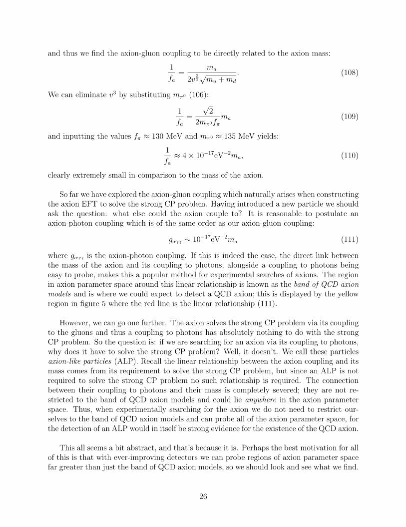
where gaγγ is the axion-photon coupling. If this is indeed the case, the direct link betweenthe mass of the axion and its coupling to photons, alongside a coupling to photons beingeasy to probe, makes this a popular method for experimental searches of axions. The regionin axion parameter space around this linear relationship is known as the band of QCD axionmodels and is where we could expect to detect a QCD axion; this is displayed by the yellowregion in figure 5 where the red line is the linear relationship (111).
However, we can go one further. The axion solves the strong CP problem via its couplingto the gluons and thus a coupling to photons has absolutely nothing to do with the strongCP problem. So the question is: if we are searching for an axion via its coupling to photons,why does it have to solve the strong CP problem? Well, it doesn’t. We call these particlesaxion-like particles (ALP). Recall the linear relationship between the axion coupling and itsmass comes from its requirement to solve the strong CP problem, but since an ALP is notrequired to solve the strong CP problem no such relationship is required. The connectionbetween their coupling to photons and their mass is completely severed; they are not re-stricted to the band of QCD axion models and could lie anywhere in the axion parameterspace. Thus, when experimentally searching for the axion we do not need to restrict our-selves to the band of QCD axion models and can probe all of the axion parameter space, forthe detection of an ALP would in itself be strong evidence for the existence of the QCD axion.
This all seems a bit abstract, and that’s because it is. Perhaps the best motivation for allof this is that with ever-improving detectors we can probe regions of axion parameter spacefar greater than just the band of QCD axion models, so we should look and see what we find.
26
QC
D a
xio
n m
odels
ALP
ALP
10-10
10-8
10-6
10-4
10-2
100
10-13
10-12
10-11
10-10
10-9
10-8
Figure 5: The axion parameter space. The red line is a plot of (111) and the yellow regiondisplays the band of QCD axion models.
This naming convention of QCD axions and ALPs can be a slightly confusing one. Weassure the reader that any previously mentioned ‘axion’ is indeed a QCD axion, however,from here onwards an ‘axion’ could refer to either a QCD axion, an ALP, or both and isdetermined from the context. To summarise:
• QCD Axion: Solves the Strong CP problem
• ALP: Does not solve the Strong CP problem
• Axion: Either or both of the above, determined by the content.
27

4 Experimental Searches For Axions
4.1 Axion-Photon Conversion
To use the axion-photon coupling as a means of detecting axions, we first need to determinethe probability of axion photon conversion. The derivation itself provides little enlightenmenttowards our goal so we demote it to appendix B and simply state the result:
P (γ → a) = P (a→ γ) =
(gaγBe
q
)2
sin2
(qL
2
). (112)
The above applies for an axion propagating along an optical cavity of length L filled withan external magnetic field of strength Be, where q is the difference between the axion andphoton wavenumbers.
The key point is that axion-photon conversion is stimulated by the presence of an externalmagnetic field Be. Thus, to best detect axions via this coupling we must construct a longoptical cavity filled with a strong magnetic field where axion-photon conversion can occurand the resulting photons can be detected.
4.2 Solar Axion Production
Axions can be produced within the solar interior via a process called the Primakoff conver-sion, where plasma photons are converted into axions due to the presence of the Coulombfield of charged particles. Although there are other production methods (such as ABC mech-anisms where the ALPs couple with electrons) the detection methods we study only considerthe Primakoff conversion channel. This channel peaks at 4.2 keV and exponentially decreasesfor higher energies, as seen in figure 6.
4.3 The Axion Helioscope
A popular tool for experimentally probing the axion is called the axion helioscope. Using asource of solar axions, they stimulate axion-photon conversion by the means of a strong lab-oratory magnet and aim to detect the resulting X-rays produced. An axion helioscope willthus consist of a powerful magnet applying a strong magnetic field to a long optical cavity(the magnets bore), where axion-photon conversion can occur. This is combined with X-raydetectors to detect such a conversion, with an optional X-ray focusing stage between themagnet and the detector to increase the signal to noise ratio. See figure 7 for a conceptualarrangement of an enhanced axion helioscope with X-ray focusing.
Aligning the optical cavity with the sun will, hopefully, yield a spike in X-ray detectiondue to solar axion production. In the event of such a spike, (112) can be used to determinegaγγ and thus measure the mass of the axion, ma. If no signal above the background isobserved upon solar alignment of the axion helioscope, a notion we will become very famil-iar with, an experimental upper bound of the axion-photon coupling gaγγ can be determined.
28

0 1 2 3 4 5 6 7 8 9 100
0.5
1
1.5
2
2.5
3
E !keV"
dΦ dE!1020 keV"1 year"1m"2 "
0 1 2 3 4 5 6 7 8 9 100
0.5
1
1.5
2
2.5
3
E !keV"
dΦ dE!1020 keV"1 year"1m"2 "
Figure 9: Solar axion flux spectra at Earth by di↵erent production mechanisms. On the left, the mostgeneric situation in which only the Primako↵ conversion of plasma photons into axions is assumed.On the right the spectrum originating from processes involving electrons, bremsstrahlung, Comptonand axio-recombination [323, 395]. The illustrative values of the coupling constants chosen are ga� =10�12 GeV�1 and gae = 10�13. Plots from [480].
(where !p is the plasma frequency of the gas, !2p = 4⇡↵ne/me, being ne and me the electron density and
the electron mass respectively). If the axion mass matches the photon mass, q = 0 and the coherence isrestored. By changing the pressure of the gas inside the pipe in a controlled manner, the photon masscan be systematically increased and the sensitivity of the experiment can be extended to higher axionmasses. In this configuration, in the event of a positive detection, helioscopes can determine the valueof ma. Even in vacuum, ma can be determined from the spectral distortion produced by the onset ofALP-photon oscillation in the helioscope of the low energy part of the spectrum, something that canbe detectable for masses down to 10�3 eV, depending of the intensity of the signal [484].
The basic layout of an axion helioscope thus requires a powerful magnet coupled to one or moreX-ray detectors. In modern incarnations of the concept, as shown in figure 10, an additional focusingstage is added at the end of the magnet to concentrate the signal photons and increase signal-to-noiseratio. When the magnet is aligned with the Sun, an excess of X-rays at the detector is expected, overthe background measured at non-alignment periods. This detection concept was first experimentallyrealised at Brookhaven National Laboratory (BNL) in 1992. A stationary dipole magnet with a field ofB = 2.2 T and a length of L = 1.8 m was oriented towards the setting Sun [38]. The experiment derivedthe upper limit ga� < 3.6 ⇥ 10�9 GeV�1 for ma < 0.03 eV at 99% C.L. At the University of Tokyo, asecond-generation experiment was built: the SUMICO axion heliscope. Not only did this experimentimplement a dynamic tracking of the Sun but it also used a more powerful magnet (B = 4 T, L = 2.3 m)than the BNL predecessor. The bore, located between the two coils of the magnet, was evacuated andhigher-performance detectors were installed [46,485,486]. This new setup resulted in an improved upperlimit in the mass range up to 0.03 eV given by ga� < 6.0⇥10�10 GeV�1 (95% C.L.). Later experimentalimprovements included the additional use of a bu↵er gas to enhance sensitivity to higher-mass axions.
A third-generation experiment, the CERN Axion Solar Telescope (CAST), began data collection in2003. The experiment uses a LHC dipole prototype magnet with a magnetic field of up to 9 T over alength of 9.3 m [488]. The magnet is able to track the Sun for several hours per day using a elevationand azimuth drive (see Fig. 11). This CERN experiment has been the first helioscope to employ X-
54
Figure 6: Solar axion flux spectra at earth assuming only the Primakoff conversion of plasmaphotons into axions. An illustrative value gaγγ = 10−12GeV−1 of the coupling constant hasbeen chosen [12].
MAGNET COIL
MAGNET COIL
B field A
L Solar
axion
flux
γ
X-ray detectors
Shielding
X-ray optics
Movable platform
Figure 10: Conceptual arrangement of an enhanced axion helioscope with X-ray focusing. Solar axionsare converted into photons by the transverse magnetic field inside the bore of a powerful magnet. Theresulting quasi-parallel beam of photons of cross sectional area A is concentrated by an appropriateX-ray optics onto a small spot area a in a low background detector. Figure taken from [487].
ray focusing optics for one of its four detector lines [489], as well as low background techniques fromdetectors in underground laboratories [490]. During its observational program from 2003 to 2011, CASToperated first with the magnet bores in vacuum (2003–2004) to probe masses ma < 0.02 eV, obtaininga first upper limit on the axion-to-photon coupling of ga� < 8.8 ⇥ 10�11 GeV�1 (95% C.L.) [396,481].The experiment was then upgraded to be operated with 4He (2005–2006) and 3He gas (2008–2011) toobtain continuous, high sensitivity up to an axion mass of ma = 1.17 eV. Data from this gas phaseprovide an average limit of ga� . 2.3 ⇥ 10�10 GeV�1 (95% C.L.), for the higher mass range of 0.02 eV< ma < 0.64 eV [483, 491] and of about ga� . 3.3 ⇥ 10�10 GeV�1 (95% C.L.) for 0.64 eV < ma < 1.17eV [492], with the exact value depending on the pressure setting.
CAST has more recently (2013-15) revisited the vacuum phase with improved detectors and anovel X-ray optics. These improvements are the outcome of R&D done in preparation of the nextgeneration axion helioscope, IAXO. In particular, one of the detection lines, dubbed IAXO pathfindersystem [493], combines for the first time both low background techniques and a new X-ray optics builtpurposely for this goal, and enjoys an e↵ective background count rate of 0.003 counts per hour in thesignal region. The outcome of this phase represents the most restrictive experimental limit to ga� formasses ma < 0.02 eV [494]:
ga� < 0.66 ⇥ 10�10GeV�1 (95% C.L.). (6.1)
CAST has been the first axion helioscope with sensitivities to ga� values below 10�10 GeV�1 andcompeting with the most stringent limits from astrophysics on this coupling, see Tab. 2. As shown inFig. 12, in the region of higher axion masses (ma & 0.1 eV), the experiment has entered the band ofQCD axion models and excluded KSVZ axions of for specific values of the axion mass in the range ma ⇠eV.
In addition to this main result, CAST has also searched for other axion production channels inthe Sun, enabled by the axion-electron or the axion-nucleon couplings. As mentioned above, in these
55
Figure 7: Conceptual arrangement of an enhanced axion helioscope with X-ray focusing.Solar axions enter the optical cavity and are converted into photons due to the appliedtransverse magnetic field. The resulting wide beam of photons are focused into a narrowbeam onto a detector [12].
Axion helioscopes need only consider the Primakoff conversion channel as this maintainsthe broadest generality and produces relevant limits on gaγγ over large mass ranges. Fora static background field, the energy of the reconverted photon is identical to that of the
29
incoming axion. We thus expect to detect the same photon energy distribution as seen forthe axions in figure 6, with the same peak at 4.2 keV (X-rays). Coherent conversion along thewhole length of the magnets bore occurs when qL � 1. For relativistic axions in vacuum,the difference between the axion and photon wavenumbers, q, is given approximately by
q = kγ − ka ≈ m2a
2ω. The coherence condition is then satisfied, for the expected solar axion
energies, with an optical cavity length of L ∼ 10m, given the axion has mass:
ma . 10−2eV. (113)
With (qL)2 ∝ m4a, the sensitivity of the experiment decreases ∼ m−4
a for larger masses.
A buffer gas can be added to the optical cavity to increase sensitivity to higher massaxions. The gas imparts an effective mass of mγ = ωp to the photons, where ωp is theplasma frequency of the gas given by:
ω2p =
4παneme
(114)
with ne and me denoting the electron number density and mass and α = 1137
is the fine struc-ture constant. If the axion mass matches the effective photon mass (ma = ωp) then q = 0and the coherence condition is restored, thus increasing the sensitivity to higher mass axions.
To help us build the most effective axion helioscope we define the figure of merit, fM ,which characterises the effectiveness of axion-photon conversion of a helioscope’s magnet.Thus, when designing an axion helioscope, maximising fM will be the main objective. Therate of axion-photon conversion is given by:
A× P (a→ γ) ∼ AB2L2 (115)
and we thus define the figure of merit as
fM := AB2L2. (116)
4.4 The Rise of the Axion Helioscope
The first axion helioscope was achieved in 1992 at the Brookhaven National Laboratory(BNL), where a stationary dipole magnet with a field of B = 2.2 T and a length of L = 1.8m was oriented towards the setting sun, hoping to detect a spike in X-rays as the sun passedover the aperture. No signal above the background was observed and thus the experimentset an upper limit of the axion photon coupling of gaγγ < 3.6 × 10⁻⁹ GeV−1 for an axionmass range of ma < 0.03 eV, and gaγγ < 7.7 × 10⁻⁹ GeV−1 for an axion mass range of0.03 eV < ma < 0.11 eV, both at 99% C.L. [13].
The second generation of axion helioscopes, SUMICO, was produced at the University ofTokyo, first achieving measurements by 1998. Improvements over the BNL axion helioscopeinclude dynamic tracking of the sun, an evacuated optical cavity of length L = 2.3 m, afar stronger applied magnetic field of B = 4 T, and higher-performance X-ray detectors.
30
SUMICO provided an upper limit of the axion photon coupling 4.5 times more stringentthan the BNL helioscope of gaγγ < 6.0 × 10⁻¹⁰GeV−1 for ma < 0.03eV at 95% C.L upondetecting no signal above the background [14].
In 2002, a buffer gas was added to the magnet’s bore to increase sensitivity to highermass axions. This allowed SUMICO to probe axions of mass 0.05 eV < ma < 0.27 eV andupon detecting no signal above the background set an upper limit of gaγγ < 6.8−10.9×10⁻¹⁰
GeV−1 at 95% C.L. [15]. By 2008, a higher mass range of 0.84 eV < ma < 1.00 eV wasprobed and set an upper limit of gaγγ < 5.6−13.4×10⁻¹⁰ GeV−1 at 95% C.L. upon detectingno signal above the background [16].
4.5 The Legacy of the CERN Axion Solar Telescope
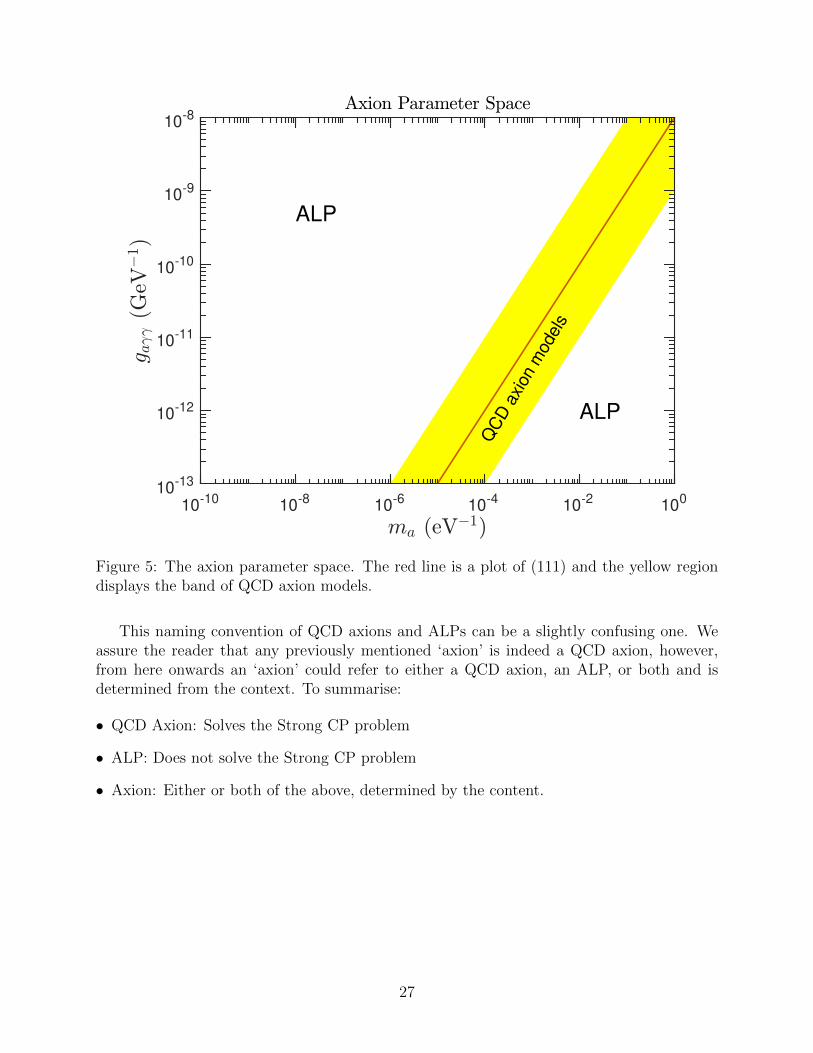
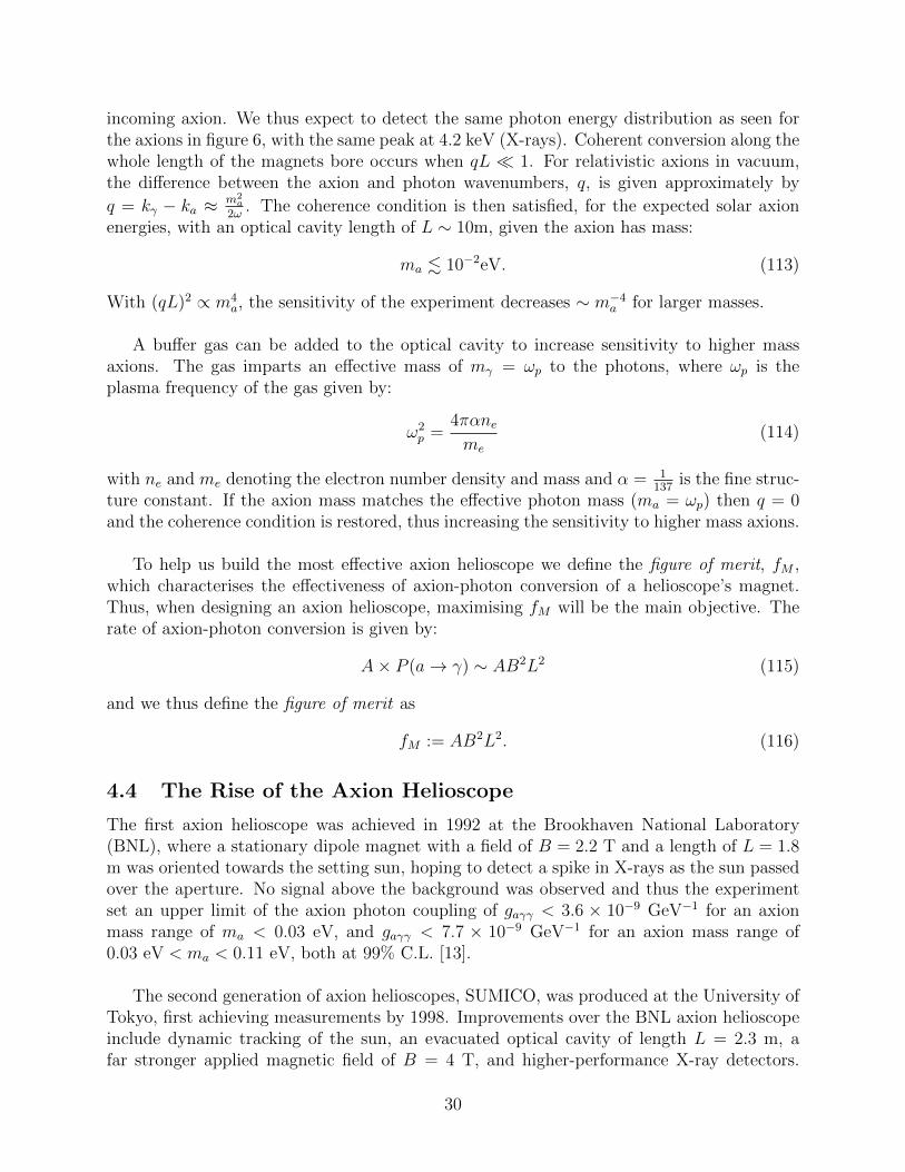
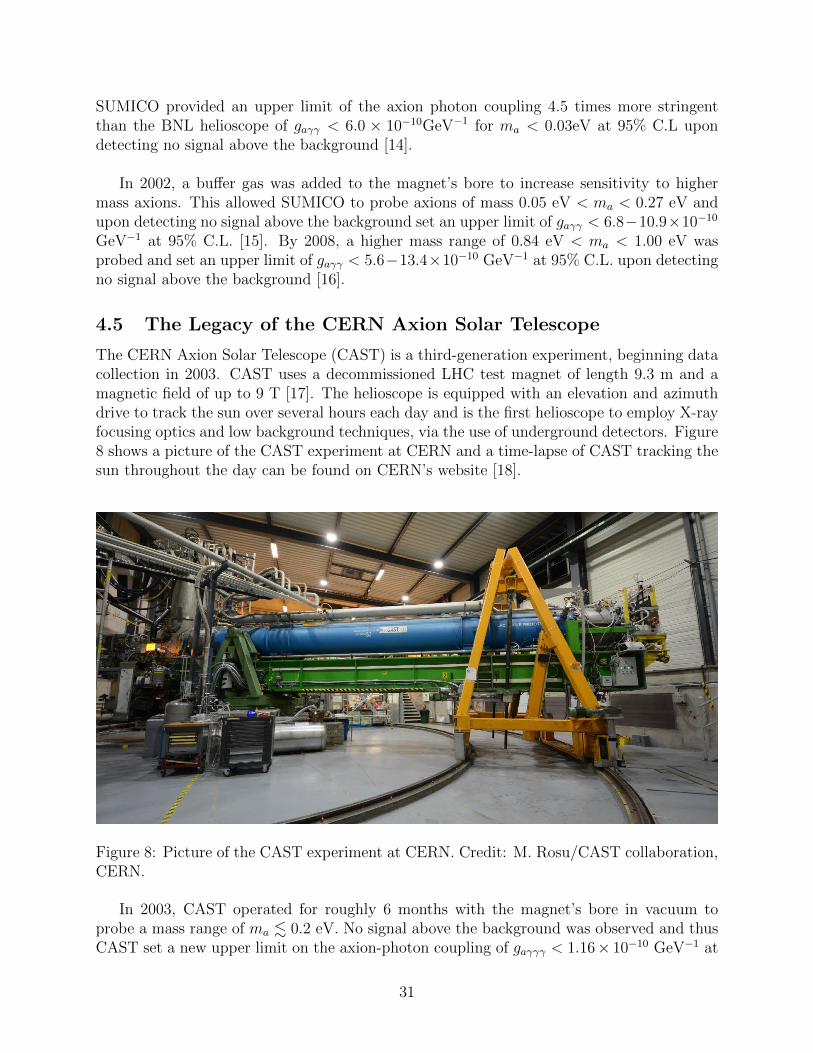
The CERN Axion Solar Telescope (CAST) is a third-generation experiment, beginning datacollection in 2003. CAST uses a decommissioned LHC test magnet of length 9.3 m and amagnetic field of up to 9 T [17]. The helioscope is equipped with an elevation and azimuthdrive to track the sun over several hours each day and is the first helioscope to employ X-rayfocusing optics and low background techniques, via the use of underground detectors. Figure8 shows a picture of the CAST experiment at CERN and a time-lapse of CAST tracking thesun throughout the day can be found on CERN’s website [18].
Figure 11: Picture of the CAST experiment at CERN. Credit: M. Rosu/CAST collaboration, CERN
cases helioscopes provide limits to the product of ga� and the corresponding coupling. More specifically,CAST has provided results on the search for :
• 14.4 keV solar axions emitted in the M1 transition of Fe-57 nuclei [495],
• MeV axions from 7Li and D(p, �)3He nuclear transitions [496],
• keV axions from the ABC processes involving the axion-electron coupling [395],
• more exotic ALP or WISP models, like chameleons [497,498]
So far each subsequent generation of axion helioscopes has resulted in an improvement in sensitivityto ga� of about a factor of a few over its predecessor (see table 5). All helioscopes so far have largely reliedon reusing existing equipment, especially the magnet. CAST in particular has enjoyed the availabilityof the first-class LHC test magnet. Going substantially beyond CAST sensitivity appears to be possibleby designing a dedicated magnet, optimised to maximise the helioscope magnet’s figure of merit fM =B2 L2 A, where B, L and A are the magnet’s field strength, length and cross sectional aperture area,respectively. fM is defined proportional to the photon signal from converted axions. Improving the valueof fM obtained by CAST can only be achieved [487] by a completely di↵erent magnet configuration witha much larger magnet aperture A, which in the case of the CAST magnet is only 3⇥10�3 m2. However,for this figure of merit to directly translate into a signal-to-noise ratio of the overall experiment, theentire cross sectional area of the magnet must be equipped with X-ray focusing optics. The layout ofthis enhanced axion helioscope, sketched in Figure 10, was proposed in [487] as the basis for IAXO, theInternational Axion Observatory.
IAXO is the next generation axion helioscope, currently at design stage. It builds upon the ex-perience of CAST, and aims at building a new large-scale magnet optimised for an axion search andextensively implementing focusing and low background techniques. Thus the central component ofIAXO is a new superconducting magnet that, contrary to previous helioscopes, will follow a toroidalmultibore configuration [502], to e�ciently produce an intense magnetic field over a large volume. Cur-rent design considers a 25 m long and 5.2 m diameter toroid assembled from 8 coils, and e↵ectivelygenerating and average (peak) 2.5 (5.1) Tesla in 8 bores of 600 mm diameter. This represents a 300
56
Figure 8: Picture of the CAST experiment at CERN. Credit: M. Rosu/CAST collaboration,CERN.
In 2003, CAST operated for roughly 6 months with the magnet’s bore in vacuum toprobe a mass range of ma . 0.2 eV. No signal above the background was observed and thusCAST set a new upper limit on the axion-photon coupling of gaγγγ < 1.16× 10⁻¹⁰ GeV−1 at
31

95% C.L. [19].
CAST was soon upgraded, operating between 2005 and 2006 with 4He contained in theoptical cavity to increase its sensitivity to higher mass axions. Within this period, CASToperated at around 160 pressure settings taking approximately 2 hours of data at each set-ting. Once again, no signal above the background was observed and thus CAST set a newupper limit of gaγγ < 2.2× 10⁻¹⁰ GeV−1 at 95% C.L. for a mass range of ma . 0.4 eV [20].
From 2008 to 2011, the 4He within the optical cavity was exchanged for 3He, allowing forhigher pressure settings and hence sensitivity to higher mass axions. CAST first operatedwith the 3He gas at T = 1.8 K, taking approximately 1 hour of data at each of the 252different pressure settings, probing an axion mass range of 0.39 eV . ma . 0.64 eV. Onceagain, no signal above the background was observed and thus set a upper limit for this massrange of gaγγ . 2.3× 10⁻¹⁰ GeV−1 (95% C.L.) [21]. CAST then went on to probe the massrange of 0.64 eV < ma < 1.17 eV and, as usual, no signal above the background was ob-served setting an upper limit for this mass range of gaγγ . 3.3×10⁻¹⁰ GeV−1 (95% C.L.) [22].
In recent years (2013 to 2014), CAST revisited the vacuum phase, once again probingthe mass range of ma . 0.2 eV. However, CAST now had the aid of improved detectors andnovel X-ray optics, courtesy of R&D for the next generation of axion helioscopes (IAXO),increasing the signal-to-noise ratio by a factor of 3 over CAST’s previous operational periods.Unfortunately, perhaps to no surprise by now, no signal above the background was observed.However, this operational period was able to set a record upper limit on the axion-photoncoupling of [23]:
gaγγ < 0.66× 10⁻¹⁰ GeV−1 (95% C.L.). (117)
Although all the expeditions of our helioscopes seem to be rather unfruitful, the upperlimit of gaγγ set by CAST’s most recent adventure really is a profound achievement; for weare now probing deep into the band of QCD axion models (111) for low mass axions. Foran axion mass of ma . 0.2 eV we currently have:
(gaγγma
)
QCD axion model
. 10−16,
(gaγγma
)
Experimental
< 3.3× 10⁻¹⁹. (118)
4.6 The International Axion Observatory: The Final Frontier
The International Axion Observatory (IAXO) is the next generation of axion helioscope, cur-rently at the design stage. Its main asset is a new, purpose-built, superconducting magnetin a toroidal multibore configuration (see figure 9) which will efficiently produce an intensemagnetic field over a large volume. Recall that, when designing an axion helioscope, ourobjective is to maximise the figure of merit fM (116), thus, there are two possible alignmentsof the bores and coils in IAXO. In the first, the bores are placed between the superconductingcoils (area maximising) and in the second, the bores are centred inside the superconducting
32

coils (field maximising). See figure 10 for a pictorial description.
E. Cryostat and Movement System
The design of the cryostat is based on a large cylinder andtwo thick end plates with eight cylindrical open bores placedin between them, see Fig. 5. The vessel is optimized to sustainthe atmospheric pressure difference and the gravitational load,while being as light and thin as possible. Using two end flangesat the vessel’s rims, as well as periodic reinforcement ribs atone meter intervals along the cryostat’s length, the structuraldesign goals are met for a 10 mm thick Al5083 vessel withtwo 70 mm thick end plates. The 10 mm wall thickness of theeight cylindrical bores have also been minimized in order forthe bores to be placed as close as possible to the racetracks’inner radius, thereby increasing the MFOM.
Searching for solar axions, the IAXO detectors need to trackthe sun for the longest possible period in order to increase thedata-taking efficiency. Thus, the magnet needs to be able torotate both horizontally and vertically by the largest possibleangles. For vertical inclination a ± 25� movement is required,while the horizontal rotation should be stretched to a full 360�
rotation before the magnet revolves back at a faster speed toits starting position.
The 250 tons magnet system will be supported at its centerof mass point (see Fig. 3), thus minimizing the torques actingon the support structure and allowing for simple rotation andinclination mechanisms. Accordingly, a set of drives can beused to rotate the magnet, while a simple inclination structurecan be placed behind the detectors (the farthest part of thesystem from its center of mass point), minimizing the forcerequired to incline the magnet. The magnet services can beconnected via a turret aligned with the rotation axis, thussimplifying the flexible cables and transfer lines arrangement.
Fig. 5. Mid-plane cut of the magnet vessel with depth view, showing the coldmass, surrounded by a thermal shield, and the cryostat. The open bores willallow for easy regular maintenance of the magnet system while simplifyingthe use of experimental instrumentation.
A 3D spiral shaped flexible chain, with radius and lengthaltering as the magnet moves, is guiding the services linesand cables to the stationary connection point.
F. Cryogenics
The coil windings are cooled by liquid helium at a temper-ature of 4.5 K via conduction. The cooling scheme utilizesa forced flow helium cooling, where the coolant flows in apipe system which will be attached to the coil casings, thusallowing for conduction cooling, in a manner similar to theATLAS toroids [6], [7]. The decision for using this conceptis following the same philosophy of our concept: a knowntechnology with a low-cost proven solution and most reliable.
The heat load on the magnet by radiation and conductionis ⇠150 W at 4.5 K. In addition comes the thermal shieldheat load of ⇠1.6 kW. An acceptable thermal design goal isto limit temperature rise in the coils to 0.1 K above the coolanttemperature under the given heat loads. To warrant this, a massflow rate of ⇠ 200 g/s is required.
A challenge is to maintain a stable forced flow againstgravity because the magnet has to rotate at both positive andnegative vertical angles. A possible solution is to use a dualcooling system, driven by a cold He-pump and a proper set ofvalves. When the magnet passes through its horizontal whiletracking the sun, the helium flow is switched from one tothe other circuit, thereby guaranteeing continuous helium flowalong the coil casings.
III. CONCLUSION
The design of the new IAXO toroidal superconductingmagnet satisfies the design criterion of increasing the solaraxion searches sensitivity by at least 1 order of magnitude.The design is relying on known engineering solutions andmanufacturing techniques. The design features maximum flex-ibility for the experimentalists, thus allowing to maximize andextend the detection potential of not only the search of axions,but also of more exotic particles, commonly known as AxionLike Particles (ALPs). Essentially, the magnet system andoptical detectors are separated, allowing for a parallel effort ofdevelopment, construction and initial operation. This, thereby,also minimizes cost and risks. In the coming years the designwill be further detailed and project funding will be proposed.
ACKNOWLEDGMENT
The authors would like to thank D. Mladenov of CERNfor thorough and useful discussions on FE analysis. Weacknowledge L. Walckiers and S. Russenschuck of CERN fordirecting the project to its current course at its early stages. Wethank I. Ortega for his contribution to the lay-out optimizationstudy. I. Shilon acknowledges the support from the SpanishMinistry of Economy and Competitiveness (MINECO) undercontract FPA2011-24058. H. Silva acknowledges the supportfrom the Portuguese Foundation for Science and Technology(FCT) under contract SFRH/BEST/51761/2011. Lastly, wethank our IAXO collaborators for motivating this work.
Figure 9: Cross-section of IAXO’s magnet and its bores in the area maximising arrangement[24]. The cold mass is surrounded by a thermal shield and a cryostat. The open bores allowfor easy regular maintenance of the magnet system.
II. DESIGN CONCEPT
A. Figure of Merit and Lay-Out Optimization
The first step towards a conceptual design of IAXO’smagnet is to optimize its toroidal geometry in order to meetthe main design criterion, namely, achieving a sensitivity tothe coupling between axions and photons of one order ofmagnitude beyond the limit of the current experiment (i.e.CAST). The magnet’s figure of merit (MFOM) is given byfM = L2B2A [5], where L is the magnet’s length, B themagnetic field and A the aperture covered by the x-ray optics.Currently, CAST’s MFOM is 21 T2m4. Translating the designcriterion to the fM language, the IAXO magnet should achievean MFOM of 300, relative to CAST. One should notice thatthe complete figure of merit of the experiment includes thetracking, detectors and optics parameters as well and is givenin [5].
(a) (b)
Fig. 2. Illustration of the two principle angular alignment options consideredfor the telescopes with respect to the coils. The rectangles represent thetoroid’s coil and the circles represent the telescopes’ bores. (a) ”Fielddominated” alignment: telescopes behind the coils. (b) ”Area dominated”alignment: telescopes between the coils.
When the magnet’s straight section length L is set to 20 m,the MFOM is determined by the integral
RB2(x, y)dxdy. The
integration is performed solely across the open area coveredby the x-ray optics. Hence, to perform the integration, thetelescopes’ positioning must be determined. Upon minimizingthe radial positioning, two principal options for the angularalignment are considered: one is to align each of the telescopesbetween each pair of racetrack coils, whereas the other is toplace the telescopes behind the racetrack coils. Fig. 2 providesa general illustration of the two alignment options for an eightcoils toroid. In practice, the two options represent two differentapproaches: the first, referred to as the ”area dominated”option, takes advantage of the entire large aperture of eachof the telescopes and the second ”field dominated” optionassumes that placing the coils behind the optics, and by thatincluding areas with higher magnetic field in the integration,will increase fM .
Once the telescopes’ position is fixed, one can performthe integration over a disc with radius Rdet centered at(Rcen, ✓cen). Then, the magnetic field is determined by themagnet’s geometrical and electromagnetic parameters. For
each lay-out configuration, the magnetic field is calculatedusing a 3D FEA model and the integration is then performedon the mid-plane. The model features an arc at the bended sec-tions of each racetrack with a radius Rarc = (Rout �Rin)/2,where Rout and Rin are the outer and inner radii of theracetrack coils, respectively. The model also assumes the useof an Al stabilized Rutherford NbTi cable in the coil windings.The winding dimensions are determined from the conductordimensions assuming a few different winding configurations.
The optimization study shows that IAXO’s MFOM is ef-fected considerably by the fraction of the telescopes’ aper-ture exposed to x-rays. Even when considering the ”fielddominated” alignment, it is preferable to use thinner coils,thus increasing the open aperture that is picked up by thetelescopes. Moreover, the ”area dominated” option gives a15% larger MFOM, compared to the ”field dominated” option.
The result of the geometrical optimization study leads toa design concept, as presented in Fig. 3, addressing all theexperimental requirements of the magnet while relying onknown and mostly well proven engineering solutions. Thisleads to a magnet design which is technically feasible to man-ufacture. Furthermore, the design concept essentially supportsthe decoupling of the magnet system from the optical detectionsystems. This allows for open bores, which are centered andaligned in between the racetrack coils, in accordance to thegeometrical study. The eight warm bores will simplify theuse of physics experimental instrumentation and the regularmaintenance of the system. The diameter of the bores matchesthe diameter of the telescopes in use.
The toroidal magnet comprises the coil and its casing, aninner cylindrical support for the magnetic forces, a thermalshield, a vacuum vessel and a movement system (see Figs. 3
Fig. 3. Schematic view of the IAXO system. Shown are the cryostat, eighttelescopes, turret leading the flexible services lines into the magnet, cryogenicsand powering services boxes, inclination system and the rails for horizontalmovement.
Figure 10: Illustration of the two possible alignments of the bores and coils in IAXO [24].The rectangles represent the toroid’s coil and the circles represent the telescopes’ bores. (a)Field maximising: Telescope bores are centred inside the superconducting coils. (b) Areamaximising: Telescope bores are placed between the superconducting coils.
The current design for the magnet is a 22 m long toroid with a 2.05 m outer radius anda 1.05 m inner radius, constructed from 8 superconducting coils generating a peak mag-
33

netic field of 5.4 T at the coil centres (relevant to the field maximising arrangement) andan average of 2.5 T in the 8 telescope bores of 0.6 m diameter (for the area maximisingarrangement) [24]. The area maximising arrangement has the largest value of fM (300 timesthat of CAST) and is thus the configuration of choice. Each of the 8 bores is equippedwith a 0.6 m diameter x-ray telescope and the project aims to use optimised optics based onthermally-formed glass substrates, similar to those used on NASA’s NuSTAR [25]. At thefocal plane of each of the optics are low background pixelated detectors to image the focusedsignal. IAXO will also feature a buffer gas phase to increase its sensitivity to higher massaxions. Figure 11 shows the conceptual design of the overall infrastructure.
The aforementioned detectors are the exact ones used in the latest iteration of CASTand consist of small gaseous chambers read by pixelised planes of microbulk Micromesh GasStructures (Micromegas). The latest generation of such detectors in CAST have achievedrecord-breaking background levels of 1.5×10⁻⁶ counts keV−1 cm−2 s−1, more than 100 timeslower than the ones obtained by the first generation of CAST detectors [26]. Values downto ∼ 10−7 counts keV−1 cm−2 s−1 have been obtained in a test bench placed undergroundin the Laboratorio Subterraneo de Canfranc (LSC) [27]. Further reducing these values to∼ 10−8 counts keV−1 cm−2 s−1 is currently being worked on, showing the good prospects ofthis technology for the future application in IAXO.
II. DESIGN CONCEPT
A. Figure of Merit and Lay-Out Optimization
The first step towards a conceptual design of IAXO’smagnet is to optimize its toroidal geometry in order to meetthe main design criterion, namely, achieving a sensitivity tothe coupling between axions and photons of one order ofmagnitude beyond the limit of the current experiment (i.e.CAST). The magnet’s figure of merit (MFOM) is given byfM = L2B2A [5], where L is the magnet’s length, B themagnetic field and A the aperture covered by the x-ray optics.Currently, CAST’s MFOM is 21 T2m4. Translating the designcriterion to the fM language, the IAXO magnet should achievean MFOM of 300, relative to CAST. One should notice thatthe complete figure of merit of the experiment includes thetracking, detectors and optics parameters as well and is givenin [5].
(a) (b)
Fig. 2. Illustration of the two principle angular alignment options consideredfor the telescopes with respect to the coils. The rectangles represent thetoroid’s coil and the circles represent the telescopes’ bores. (a) ”Fielddominated” alignment: telescopes behind the coils. (b) ”Area dominated”alignment: telescopes between the coils.
When the magnet’s straight section length L is set to 20 m,the MFOM is determined by the integral
RB2(x, y)dxdy. The
integration is performed solely across the open area coveredby the x-ray optics. Hence, to perform the integration, thetelescopes’ positioning must be determined. Upon minimizingthe radial positioning, two principal options for the angularalignment are considered: one is to align each of the telescopesbetween each pair of racetrack coils, whereas the other is toplace the telescopes behind the racetrack coils. Fig. 2 providesa general illustration of the two alignment options for an eightcoils toroid. In practice, the two options represent two differentapproaches: the first, referred to as the ”area dominated”option, takes advantage of the entire large aperture of eachof the telescopes and the second ”field dominated” optionassumes that placing the coils behind the optics, and by thatincluding areas with higher magnetic field in the integration,will increase fM .
Once the telescopes’ position is fixed, one can performthe integration over a disc with radius Rdet centered at(Rcen, ✓cen). Then, the magnetic field is determined by themagnet’s geometrical and electromagnetic parameters. For
each lay-out configuration, the magnetic field is calculatedusing a 3D FEA model and the integration is then performedon the mid-plane. The model features an arc at the bended sec-tions of each racetrack with a radius Rarc = (Rout �Rin)/2,where Rout and Rin are the outer and inner radii of theracetrack coils, respectively. The model also assumes the useof an Al stabilized Rutherford NbTi cable in the coil windings.The winding dimensions are determined from the conductordimensions assuming a few different winding configurations.
The optimization study shows that IAXO’s MFOM is ef-fected considerably by the fraction of the telescopes’ aper-ture exposed to x-rays. Even when considering the ”fielddominated” alignment, it is preferable to use thinner coils,thus increasing the open aperture that is picked up by thetelescopes. Moreover, the ”area dominated” option gives a15% larger MFOM, compared to the ”field dominated” option.
The result of the geometrical optimization study leads toa design concept, as presented in Fig. 3, addressing all theexperimental requirements of the magnet while relying onknown and mostly well proven engineering solutions. Thisleads to a magnet design which is technically feasible to man-ufacture. Furthermore, the design concept essentially supportsthe decoupling of the magnet system from the optical detectionsystems. This allows for open bores, which are centered andaligned in between the racetrack coils, in accordance to thegeometrical study. The eight warm bores will simplify theuse of physics experimental instrumentation and the regularmaintenance of the system. The diameter of the bores matchesthe diameter of the telescopes in use.
The toroidal magnet comprises the coil and its casing, aninner cylindrical support for the magnetic forces, a thermalshield, a vacuum vessel and a movement system (see Figs. 3
Fig. 3. Schematic view of the IAXO system. Shown are the cryostat, eighttelescopes, turret leading the flexible services lines into the magnet, cryogenicsand powering services boxes, inclination system and the rails for horizontalmovement.
Figure 11: Schematic view of IAXO. Shown are the cryostat, eight telescopes, turret leadingthe flexible services lines into the magnet, cryogenics and powering services boxes, inclinationsystem, and the rails for horizontal movement [24].
Putting all the discussed values together, IAXO is expected to improve the CAST signal-
34
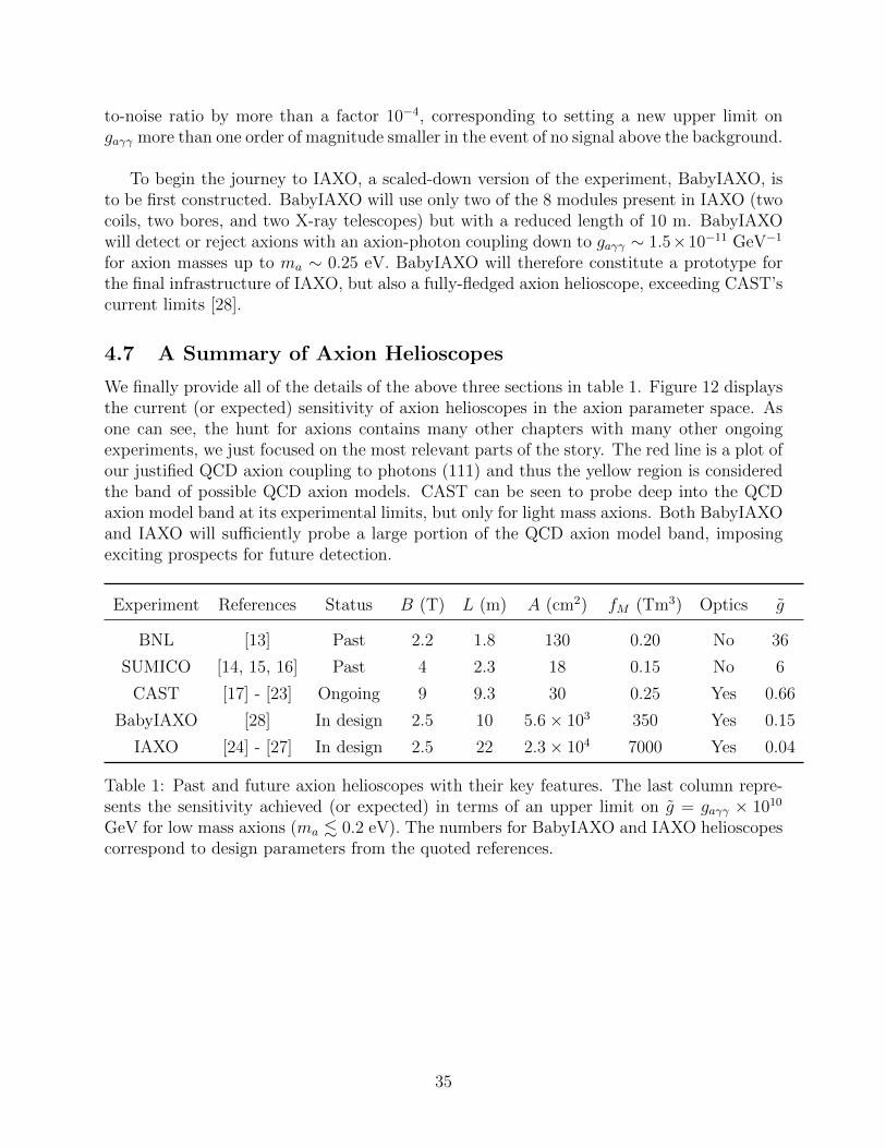
to-noise ratio by more than a factor 10−4, corresponding to setting a new upper limit ongaγγ more than one order of magnitude smaller in the event of no signal above the background.
To begin the journey to IAXO, a scaled-down version of the experiment, BabyIAXO, isto be first constructed. BabyIAXO will use only two of the 8 modules present in IAXO (twocoils, two bores, and two X-ray telescopes) but with a reduced length of 10 m. BabyIAXOwill detect or reject axions with an axion-photon coupling down to gaγγ ∼ 1.5×10⁻¹¹ GeV−1
for axion masses up to ma ∼ 0.25 eV. BabyIAXO will therefore constitute a prototype forthe final infrastructure of IAXO, but also a fully-fledged axion helioscope, exceeding CAST’scurrent limits [28].
4.7 A Summary of Axion Helioscopes
We finally provide all of the details of the above three sections in table 1. Figure 12 displaysthe current (or expected) sensitivity of axion helioscopes in the axion parameter space. Asone can see, the hunt for axions contains many other chapters with many other ongoingexperiments, we just focused on the most relevant parts of the story. The red line is a plot ofour justified QCD axion coupling to photons (111) and thus the yellow region is consideredthe band of possible QCD axion models. CAST can be seen to probe deep into the QCDaxion model band at its experimental limits, but only for light mass axions. Both BabyIAXOand IAXO will sufficiently probe a large portion of the QCD axion model band, imposingexciting prospects for future detection.
Experiment References Status B (T) L (m) A (cm2) fM (Tm3) Optics g
BNL [13] Past 2.2 1.8 130 0.20 No 36
SUMICO [14, 15, 16] Past 4 2.3 18 0.15 No 6
CAST [17] - [23] Ongoing 9 9.3 30 0.25 Yes 0.66
BabyIAXO [28] In design 2.5 10 5.6× 10³ 350 Yes 0.15
IAXO [24] - [27] In design 2.5 22 2.3× 10⁴ 7000 Yes 0.04
Table 1: Past and future axion helioscopes with their key features. The last column repre-sents the sensitivity achieved (or expected) in terms of an upper limit on g = gaγγ × 1010
GeV for low mass axions (ma . 0.2 eV). The numbers for BabyIAXO and IAXO helioscopescorrespond to design parameters from the quoted references.
35

ma(eV)10�10 10�9 10�8 10�7 10�6 10�5 10�4 10�3 10�2 10�1 1
|g a�|(G
eV�
1)
10�13
10�12
10�11
10�10
10�9
QCD
axio
nm
odels
CAST
BabyIAXO
IAXOIAXO+
ALPSIIHESS
T Hint
SN19
87A
Ferm
iSN
pros
pec
ts
Fermi NG1275
KSV
Z
HB
AMELIE
HB hint
Figure 12: Latest excluded region in the (ga�, ma) from helioscopes (CAST), as well as prospects fromfuture experiments, most relevantly from BabyIAXO and IAXO. Also shown are the prospects at highmass from a possible implementation of the AMELIE concept. Also shown are prospects from theALP-II experiment and hinted regions from astrophysics as explained in the text.
Discussions are ongoing to explore how this project could constitute a pathfinder experiment for thefuture IAXO.
6.2 Other techniques to search for solar axions
6.2.1 Primako↵-Bragg conversion in crystalline detectors
Axion-photon conversion (and viceversa) can also happen in the atomic electromagnetic field insidematerials. In the case of crystalline media, the periodic structure of the field imposes a Bragg condition,i.e., the conversion is coherently enhanced if the momentum of the incoming particle matches one of theBragg angles [511,512] (similar Laue-like conversion in crystals is studied in [513]). This concept has beenapplied to the search for solar axions with crystalline detectors [514, 515]. The continuous variation ofthe relative incoming direction of the axions with respect to the crystal planes, due to the Earth rotation,produces very characteristic sharp energy- and time-dependent patterns in the expected signal in thedetector, which can be used to e↵ectively identify a putative signal over the detector background. Thistechnique has the advantage that can be used as a byproduct of ongoing low-background undergrounddetectors (e.g. those in WIMP or double-beta decay experiments) provided they have low enough
58
Figure 12: The current (or expected) sensitivity of axion helioscopes in the axion parameterspace. The yellow band displays the region of QCD axion models [12].
5 Epilogue
We have achieved much in our journey. Recall it all began with our freedom to add a termto the QCD Lagrangian (parameterised by θ) that allows for CP-violating interactions. Ourfirst inkling of a problem is that no such CP-violating interactions have ever been observedin a strongly interacting experiment. Our first piece of evidence was the differing of the pionmasses by the parameter θ, and since the pions are of roughly equal mass suggest that θ mustbe small. Our second piece of evidence was the calculation of the neutron eDM, yielding avalue (in terms of θ) that is far larger than we experimentally measure it to be, once againtelling us that θ must be small. These two pieces of evidence instruct us to add somethinginto our theory that will dynamically set the parameter θ to zero, a new particle called theaxion. We then discussed experimental probes of the axion, and although they seemed to berather unfruitful, we will very soon be covering a huge section of axion parameter space andprobe deep into the band of QCD axion models. It truly is an exciting time to be an axion.
36
References
[1] Lev Landau. On the conservation laws for weak interactions. Nuclear Physics. 3 (1):127–131 (1957).
[2] Scott Dodelson. How do we know that distant galaxies are composed of matter rather thananti-matter? If equal quantities of each were produced in the big bang, might not someparts of the universe contain primarily matter and other parts primarily anti-matter?.Scientific American (1999).
[3] Mark Srednicki. Quantum Field Theory. ISBN: 9780511267208 (2006).
[4] Michael E. Peskin and Daniel V. Schroder. An Introduction to Quantum Field Theory.ISBN: 978-0-367-32056-0 (1995).
[5] C.A. Baker et al. Improved experimental limit on the electric dipole moment of the neu-tron. arXiv:hep-ex/0602020 (2006).
[6] Anson Hook. TASI Lectures on the Strong CP Problem and Axions. arXiv:1812.02669[hep-ph] (2018).
[7] Kazuo Fujikawa. Path-Integral Measure for Gauge-Invariant Fermion Theories. Physicalreview letters, volume 42, number 18 (1979).
[8] Jeffrey Goldstone, Abdus Salam, and Steven Weinberg. Broken Symmetries. PhysicalReview. 127 (3): 965–970 (1962).
[9] Particle Data Group: Decay constants of charged pseudoscalar mesons (2012).
[10] Mark Srednicki. Axion couplings to matter: (I). CP-conserving parts. Nucl. Phys. B260,689 (1985).
[11] M. P. Mendenhall et al. Precision measurement of the neutron β-decay asymmetry Phys.Rev. C, 87 032501 (2013).
[12] I. G. Irastorza and J. Redondo. New experimental approaches in the search for axion-likeparticles. arXiv:1801.08127 [hep-ph] (2018).
[13] D. M. Lazarus et al. A Search for solar axions. Phys. Rev. Lett. 69 2333–2336 (1992).
[14] S. Moriyama et al. Direct search for solar axions by using strong magnetic field andX-ray detectors. arXiv:hep-ex/9805026 (1998).
[15] Y. Inoue et al. Search for solar axions with mass around 1 eV using coherent conversionof axions into photons. arXiv:0806.2230 [astro-ph] (2002).
[16] Y. Inoue et al. Search for solar axions with mass around 1 eV using coherent conversionof axions into photons. arXiv:0806.2230 [astro-ph] (2008).
[17] M. Kuster et al. The X-ray Telescope of CAST. arXiv:physics/0702188 (2007).
37
[18] https://videos.cern.ch/record/2053255
[19] CAST Collaboration, K. Zioutas et al. First results from the CERN Axion Solar Tele-scope (CAST). arXiv:hep-ex/0411033 (2005).
[20] CAST Collaboration. E. Arik et al. Probing eV-scale axions with CAST.arXiv:0810.4482 [hep-ex] (2009).
[21] CAST Collaboration. M. Arik et al. Search for sub-ev mass solar axions by the cernaxion solar telescope with 3He buffer gas. arXiv:1106.3919 [hep-ex] (2012).
[22] CAST Collaboration. M. Arik, et al. CAST solar axion search with 3He buffer gas:Closing the hot dark matter gap. arXiv:1307.1985 [hep-ex] (2014).
[23] CAST Collaboration. V. Anastassopoulos et al. New CAST Limit on the Axion-PhotonInteraction. arXiv:1705.02290 [hep-ex] (2017).
[24] I. Shilon, A. Dudarev, H. Silva, and H. Kate. Conceptual Design of a New Large Super-conducting Toroid for IAXO, the New International AXion Observatory. arXiv:1212.4633[physics.ins-det] (2012).
[25] F. A. Harrison et al. The nuclear spectroscopic telescope array (nustar) high-energy x-raymission. 2013 ApJ 770 103 (2013).
[26] S. Aune et al. Low background x-ray detection with Micromegas for axion research.arXiv:1310.3391 [physics.ins-det] (2013).
[27] I. G. Irastorza et al. Gaseous time projection chambers for rare event detection: Resultsfrom the T-REX project. II. Dark matter. arXiv:1512.06294 [physics.ins-det] (2016).
[28] A. Abeln et al. Conceptual Design of BabyIAXO, the intermediate stage towards theInternational Axion Observatory. arXiv:2010.12076 [physics.ins-det] (2021).
38
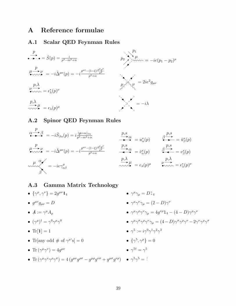
A Reference formulae
A.1 Scalar QED Feynman Rules
p
= S(p) = ip2−m2+iε
pµ ν
= −i∆µν(p) = −igµν−(1−ξ) pµpν
p2
p2+iε
p,λν
= ε∗λ(p)ν
p,λµ
= ελ(p)µ
p1
p2µ
= −ie(p1 − p2)µ
µ ν= 2ie2gµν
= −iλ
A.2 Spinor QED Feynman Rules
pα β
= −iSβα(p) = i(/p+m)βαp2−m2+iε
pµ ν
= −i∆µν(p) = −igµν−(1−ξ) pµpν
p2
p2+iε
µ α
β
= −ieγµαβ
p,sα
= usα(p)
p,sβ
= usβ(p)p,s
α= vsα(p)
p,sβ
= vsβ(p)
p,λµ
= ελ(p)µ
p,λν
= ε∗λ(p)ν
A.3 Gamma Matrix Technology
• {γµ, γν} = 2gµν14
• gµνgµν = D
• /A := γµAµ
• (γµ)† = γ0γµγ0
• Tr[1] = 1
• Tr[any odd # of γµ’s] = 0
• Tr (γµγν) = 4gµν
• Tr (γµγνγργσ) = 4 (gµνgρσ − gµρgνσ + gµσgνρ)
• γµγµ = D14
• γµγνγµ = (2−D)γν
• γµγργνγµ = 4gνρ14 − (4−D)γργν
• γµγσγργνγµ = (4−D)γσγργν−2γνγργσ
• γ5 := iγ0γ1γ2γ3
• {γ5, γµ} = 0
• γ5† = γ5
• γ5γ5 = 1
39
B Axion-Photon Conversion Probability Derivation
The Lagrangian for an interacting system of axions, photons, and EM currents is given by
L =1
2∂µa∂
µa− 1
2m2
aa2 − 1
4F µνFµν − gaγγaF µνFµν − JµAµ (119)
where −JµAµ is the electromagnetic source term with the electric 4-current Jµ = (ρ,J). Theelectric and magnetic fields are then explicitly given by:
E = −∇A0 − A, B = ∇×A. (120)
Applying the Euler-Lagrange equations to (119) yields the equations of motion:
∂µFµν = Jν − gaγF µν∂µa
(∂µ∂
µ +m2a
)a = −gaγ
4FµνF
µν .(121)
The first equation is a modification of Gauss’ and Ampere’s laws in the presence of axions
and amounts to the addition of the extra current Jνa ≡ −gaγ∂µ(F µνa
)= −gaγF µν∂µa. The
second equation is something totally new, the equation of motion of the axions. Writing thesein terms of the electric and magnetic fields yields something rather familiar, yet different;the ALP-Maxwell equations:
∇ · E = ρ− gaγB ·∇a,
∇×B− E = J + gaγ(Ba− E×∇a)
∇ ·B = 0
∇× E + B = 0
a−∇2a+m2aa = gaγE ·B.
(122)
When trying to detect axion photon conversion, a long optical cavity in a constant appliedmagnetic field is commonly used. Thus we may take B as a constant and the ALP-Maxwellequations (122) become linear and can be solved via a plane wave ansatz. Aligning our opticalcavity along the z-direction, consider the ansatz for plane waves of frequency ω propagating
40

along the cavity in the z−direction:
a
iA‖
iA⊥
∝
cosϑ
− sinϑ
0
e−i(ωt−k
′az) (ALP− like)
a
iA‖
iA⊥
∝
sinϑ
cosϑ
0
e−i(ωt−k
′γz) ( photon − like)
a
iA‖
iA⊥
∝
0
0
1
e−i(ωt−kγz) ( photon )
(123)
where A := Eiω
, A‖ has polarisation parallel to z, A⊥ has polarisation perpendicular to bothz and B, k′a and k′γ are modified wavenumbers, and ϑ is the mixing angle. We seem to havearbitrarily snuck in the notion of ALP-photon mixing, but it is evidently present due to theinteraction term in the Lagrangian (119). In a background B field, neither photons nor ALPscorrespond to freely propagating particles because the gaγγ interaction acts as a non-diagonalmass term and quantum mechanically mixes ALPs with photons with polarisation along B.The mixing angle and modified wavenumbers are given by:
tanϑ =2gaγBeω
∆k2 +√
(∆k2)2 + (2gaγBeω)2
k′2aγ
=1
2
(k2γ + k2
a ∓√
(∆k2)2 + (2gaγBeω)2
) (124)
where ∆k2 := k2γ − k2
a. Substituting this ansatz into (122) yields the solutions:
E‖(t, z) = E‖,0e−i(ωt−k′γz)
[cos2 ϑ+ e−iq
′z sin2 ϑ]
a(t, z) =E0
ωe−i(ωt−k
′az) sinϑ cosϑ
[eiq′z − 1
] (125)
where q′ := k′γ − k′a. The component of the electromagnetic wave polarised perpendicularto the external B field will of course propagate as a standard electromagnetic wave withelectric field
E⊥(t, z) = E0e−i(ωt−kγz). (126)
The particle number densities of the photons and axions are given by
|Ex|22ω
,ω|a|2
2(127)
41

respectively. As we move away from z = 0, the particle number densities of axions andphotons change, but the total flux remains constant, which we can consider to be ALP-photon oscillation. The conversion probability at some distance z is thus given by
P (γ → a)(z) =|a(z)|2|Ax(z)|2 =
∣∣∣sinϑ cosϑ[eiq′z − 1
]∣∣∣2
= sin2(2ϑ) sin2
(q′z
2
). (128)
We can make two simplifying assumptions, small mixing (ϑ � 1) and the relativisticlimit (∆k2 ≈ 2ωq). We also note that, so long as we impose E(z = 0) = 0, taking ϑ → −ϑtakes us from ALP-like to photon-like in (122). Since the transition probability is unchangedby ϑ→ −ϑ, photon to ALP oscillation probability upon propagating a distance z is equal tothe ALP to photon oscillation probability. Thus in our simplifying limits, the probability ofconversion for an axion propagating along an optical cavity of length L filled with a magneticfield of strength Be is:
P (γ → a) = P (a→ γ) =
(gaγBe
q
)2
sin2
(qL
2
). (129)
42