masigpro user’s guide - bioconductorbioconductor.org/.../inst/doc/masigprousersguide.pdfmasigpro...

maSigPro User’s Guide

Ana Conesa and Marıa J. Nueda

4 September 2017

1. Centro de Investigacion Principe Felipe, Valencia, [email protected]

2. Departamento de Matematicas, Universidad de Alicante, [email protected]

Contents

1 Introduction 2

2 Getting started 2

3 Multiple Series Time Course Experiment 23.1 Defining the regression model . . . . . . . . . . . . . . . . . . . . . . . . . . . . 53.2 Finding significant genes . . . . . . . . . . . . . . . . . . . . . . . . . . . . . . . 53.3 Finding significant differences . . . . . . . . . . . . . . . . . . . . . . . . . . . . 53.4 Obtaining lists of significant genes . . . . . . . . . . . . . . . . . . . . . . . . . 6

4 Graphical display 74.1 Venn Diagrams . . . . . . . . . . . . . . . . . . . . . . . . . . . . . . . . . . . . 74.2 see.genes() . . . . . . . . . . . . . . . . . . . . . . . . . . . . . . . . . . . . . 74.3 PlotGroups() . . . . . . . . . . . . . . . . . . . . . . . . . . . . . . . . . . . . . 84.4 PlotProfiles() . . . . . . . . . . . . . . . . . . . . . . . . . . . . . . . . . . . 11

5 Other designs 115.1 Single Series Time Course . . . . . . . . . . . . . . . . . . . . . . . . . . . . . . 115.2 Common Starting Time . . . . . . . . . . . . . . . . . . . . . . . . . . . . . . . 12

6 Next Generation-Sequencing series 13

7 Iso-maSigPro: analysis of alternative isoform expression in time coursetranscriptomics experiments 157.1 IsoModel() and getDS() . . . . . . . . . . . . . . . . . . . . . . . . . . . . . . 157.2 Clustering strategy: seeDS() and tableDS() . . . . . . . . . . . . . . . . . . . 177.3 PodiumChange() . . . . . . . . . . . . . . . . . . . . . . . . . . . . . . . . . . . 197.4 IsoPlot() . . . . . . . . . . . . . . . . . . . . . . . . . . . . . . . . . . . . . . . 20

1

1 Introduction

maSigPro is a R package that initially was developed for the analysis of single and multiseriestime course microarray experiments (Conesa et al., 2006). maSigPro has been adapted todeal also with Next Generation-Sequencing (NGS) series of data in a proper way (Nuedaet al., 2014). The usage of this opcion is explained in 6 section.maSigPro also includes several tools for the analysis of alternative isoform expression in timecourse transcriptomics experiments. In 7 section the usage of this opcion is explained.maSigPro follows a two steps regression strategy to find genes with significant temporalexpression changes and significant differences between experimental groups. The method de-fines a general regression model for the data where the experimental groups are identified bydummy variables. The procedure first adjusts this global model by the least-squared techniqueto identify differentially expressed genes and selects significant genes applying false discov-ery rate control procedures. Secondly, stepwise regression is applied as a variable selectionstrategy to study differences between experimental groups and to find statistically significantdifferent profiles. The coefficients obtained in this second regression model will be useful tocluster together significant genes with similar expression patterns and to visualize the results.This document is a example-based guide for the use of maSigPro. We recommend to opena R sesion and go through this tutorial running the code given at the different sections. Theguide does not provide a detailed description of the functions of the package or demonstratesthe statistical basis of the methodology. The later is described in the work by (Conesa et al.,2006) and (Nueda et al., 2014).

2 Getting started

The maSigPro package can be obtained from the Bioconductor repository or downloadedfrom http://www.ua.es/personal/mj.nueda and http://bioinfo.cipf.es/downloads. LoadmaSigPro by typing at the R prompt:

> library(maSigPro) # load maSigPro library

The on-line help of maSigPro can be started by typing at the R prompt:

>help(package="maSigPro") #for package help

>?p.vector #for function help

The analysis approach implemented in maSigPro is executed in 5 major steps (Figure 1)which are run by the package core functions make.design.matrix(), p.vector(), T.fit(),get.siggenes() and see.genes(). Additionally, the package provides the wrapping functionmaSigPro() which executes the entire analysis in one go.In the following section we will explain the usage of each of these funcions using as example adata set from a multiple series time course experiment. At the end of this document we willalso explain how to apply maSigPro to other experimental designs.

3 Multiple Series Time Course Experiment

For this section we will use a public data set from a plant abiotic stress study performed atthe TIGR Institute by (Rensink et al., 2005). In this study, potato plants were subjected

2

http://www.ua.es/personal/mj.nueda

http://bioinfo.cipf.es/downloads

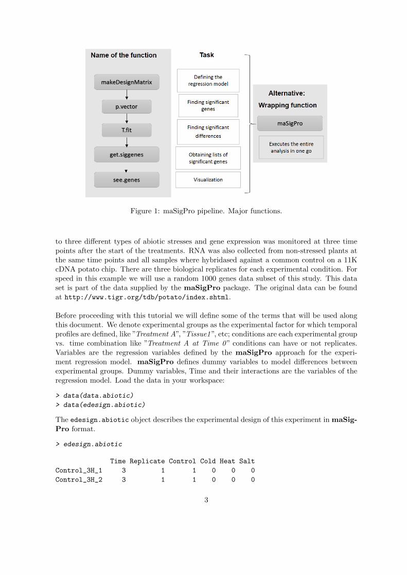
Figure 1: maSigPro pipeline. Major functions.

to three different types of abiotic stresses and gene expression was monitored at three timepoints after the start of the treatments. RNA was also collected from non-stressed plants atthe same time points and all samples where hybridased against a common control on a 11KcDNA potato chip. There are three biological replicates for each experimental condition. Forspeed in this example we will use a random 1000 genes data subset of this study. This dataset is part of the data supplied by the maSigPro package. The original data can be foundat http://www.tigr.org/tdb/potato/index.shtml.

Before proceeding with this tutorial we will define some of the terms that will be used alongthis document. We denote experimental groups as the experimental factor for which temporalprofiles are defined, like ”Treatment A”, ”Tissue1”, etc; conditions are each experimental groupvs. time combination like ”Treatment A at Time 0” conditions can have or not replicates.Variables are the regression variables defined by the maSigPro approach for the experi-ment regression model. maSigPro defines dummy variables to model differences betweenexperimental groups. Dummy variables, Time and their interactions are the variables of theregression model. Load the data in your workspace:

> data(data.abiotic)

> data(edesign.abiotic)

The edesign.abiotic object describes the experimental design of this experiment in maSig-Pro format.

> edesign.abiotic

Time Replicate Control Cold Heat Salt

Control_3H_1 3 1 1 0 0 0

Control_3H_2 3 1 1 0 0 0

3

http://www.tigr.org/tdb/potato/index.shtml

Control_3H_3 3 1 1 0 0 0

Control_9H_1 9 2 1 0 0 0

Control_9H_2 9 2 1 0 0 0

Control_9H_3 9 2 1 0 0 0

Control_27H_1 27 3 1 0 0 0

Control_27H_2 27 3 1 0 0 0

Control_27H_3 27 3 1 0 0 0

Cold_3H_1 3 4 0 1 0 0

Cold_3H_2 3 4 0 1 0 0

Cold_3H_3 3 4 0 1 0 0

Cold_9H_1 9 5 0 1 0 0

Cold_9H_2 9 5 0 1 0 0

Cold_9H_3 9 5 0 1 0 0

Cold_27H_1 27 6 0 1 0 0

Cold_27H_2 27 6 0 1 0 0

Cold_27H_3 27 6 0 1 0 0

Heat_3H_1 3 7 0 0 1 0

Heat_3H_2 3 7 0 0 1 0

Heat_3H_3 3 7 0 0 1 0

Heat_9H_1 9 8 0 0 1 0

Heat_9H_2 9 8 0 0 1 0

Heat_9H_3 9 8 0 0 1 0

Heat_27H_1 27 9 0 0 1 0

Heat_27H_2 27 9 0 0 1 0

Heat_27H_3 27 9 0 0 1 0

Salt_3H_1 3 10 0 0 0 1

Salt_3H_2 3 10 0 0 0 1

Salt_3H_3 3 10 0 0 0 1

Salt_9H_1 9 11 0 0 0 1

Salt_9H_2 9 11 0 0 0 1

Salt_9H_3 9 11 0 0 0 1

Salt_27H_1 27 12 0 0 0 1

Salt_27H_2 27 12 0 0 0 1

Salt_27H_3 27 12 0 0 0 1

Note that arrays are given in rows and experiment descriptors are provided in columns. Thefirst column shows the value that variable Time takes in each array. Replicates columnis an index column that indicates the replicated arrays: all arrays belonging to the sameexperimental condition must be given the same number. The remaining columns are binarycolumns that give the assignment of arrays to experimental groups. There are as many binarycolumns as experimental groups and arrays take the value 1 or 0 whether they belong or notto that experimental group.The data.abiotic object is a matrix with normalized gene expression data. Genes mustbe in rows and arrays in columns. maSigPro uses row and colunm names of the data andedesign objects throughout the package. Array names are the labels of the rows of the edesignobject and columns of the data object that must be in the same order. GeneIDs are the labelsof the rows in the data object. And experiment descriptors are put in the column names of

4

the edesign object.

> colnames(data.abiotic)

> rownames(edesign.abiotic)

> colnames(edesign.abiotic)

> rownames(data.abiotic)

3.1 Defining the regression model

Create a regression matrix for the full regression model:

> design <- make.design.matrix(edesign.abiotic, degree = 2)

This example has three time points, so we can consider up to a quadratic regression model(degree = 2). Larger number of time points would potentially allow a higher polynomial de-gree. design is a list. Its element dis is the actual regression design matrix. groups.vectorcontains the assignment of regression variables to experimental groups.

> design$groups.vector

[1] "ColdvsControl" "HeatvsControl" "SaltvsControl" "Control"

[5] "ColdvsControl" "HeatvsControl" "SaltvsControl" "Control"

[9] "ColdvsControl" "HeatvsControl" "SaltvsControl"

3.2 Finding significant genes

The next step is to compute a regression fit for each gene. This is done by the functionp.vector(). This function also computes the p-value associated to the F -Statistic of themodel, which is used to select significant genes. By default maSigPro corrects this p-valuefor multiple comparisons by applying the linear step-up (B-H) false discovery rate (FDR) pro-cedure (Benjamini and Hochberg, 1995). This procedure can be modified by choosing anotheroption of the p.adjust function that is controlled by the function parameter MT.adjust ofp.vector. The level of FDR control is given by the function parameter Q.

> fit <- p.vector(data.abiotic, design, Q = 0.05, MT.adjust = "BH", min.obs = 20)

p.vector() returns a list of values:

> fit$i # returns the number of significant genes

> fit$alfa # gives p-value at the Q false discovery control level

> fit$SELEC # is a matrix with the significant genes and their expression values

3.3 Finding significant differences

Once significant genes have been found, maSigPro applies a variable selection procedure tofind significant variables for each gene. This will ultimatelly be used to find which are theprofile differences between experimental groups. This step is done by the T.fit() function.

> tstep <- T.fit(fit, step.method = "backward", alfa = 0.05)

5

T.fit() executes stepwise regression. The step.method can be ”backward” or ”forward” in-dicating whether the step procedure starts from the model with all or none variables. Usemethod ”two.ways.backward” and ”two.ways.forward” to allow variables to both get in andout. At each regression step the p-value of each variable is computed and variables get in/outthe model when this p-value is lower or higher than the given cut-off value alfa. tstep is alsoa list. Its element sol is a matrix of statistical results obtained by the stepwise regression.For each selected gene the following values are given:

p-value of the regression ANOVA

R-squared of the model

p-value of the regression coefficients of the selected variables

3.4 Obtaining lists of significant genes

The following step is to generate lists of significant genes according to the way we want to seeresults. This is done by the function get.siggenes(). This function has two major arguments,rsq and vars.

rsq: is a cutt-off value for the R-squared of the regression model.

vars: is used to indicate how to group variables to show results. There are 3 possible values:

groups: This will generate a list of significant genes for each experimental group.The list corresponding to the reference group will contain genes whose expressionprofile is significantly different from a 0 profile. The lists corresponding to theremaining experimental groups will contain genes whose profiles are different fromthe reference group.

all: One unique list of significant genes a any model variable will be produced.

each: There will be as many lists as variables in the regression model. This can beused to analyze specific differences, for example genes that have linear or saturationkinetics.

> sigs <- get.siggenes(tstep, rsq = 0.6, vars = "groups")

> names(sigs)

[1] "sig.genes" "summary"

The element summary is a data frame containing the significant genes for the selected vars.The element sig.genes is a list with all the information needed for the graphical displayexplained in the following section.You can further explore your results by:

> names(sigs$sig.genes)

[1] "Control" "ColdvsControl" "HeatvsControl" "SaltvsControl"

> names(sigs$sig.genes$ColdvsControl)

[1] "sig.profiles" "coefficients" "group.coeffs" "sig.pvalues"

[5] "g" "edesign" "groups.vector"

6

1

1

2

987

26

101

ColdvsControl

HeatvsControl

SaltvsControl

15

47

17

71

1

2

4

40

9

30

Control

ColdvsControl HeatvsControl

SaltvsControl

(a) (b)

Figure 2: (a) Venn Diagram for Cold, Heat and Salt stress significant genes. (b) Venn Diagramadding also the Control group.

4 Graphical display

maSigPro has several functions for the visual exploration of the results: Venn diagrams,profiles of specific genes and profiles of groups of genes from different perspectives. The mainprincipal function is see.genes that makes a clustering anlaysis and call PlotProfiles andPlotGroups functions to visualize the clusters.

4.1 Venn Diagrams

suma2Venn() function displays the summary result, obtained with get.siggenes() function,as a Venn diagram. This can be a first view of the obtained results.Figure 2 shows 2 Venn diagrams made with the following commands. The first one is a Venndiagram of the significant genes for the three stress experimental groups and the second oneincludes also the control group.

> suma2Venn(sigs$summary[, c(2:4)])

> suma2Venn(sigs$summary[, c(1:4)])

4.2 see.genes()

Use see.genes() to visualize the result of a group of genes, for example, to visualize thesignificant genes obtained as significant in the previous step in ControlvsSalt, that are geneswith significant differences between Salt and Control gene expression.

7

> sigs$sig.genes$SaltvsControl$g

[1] 191

see.genes(sigs$sig.genes$ColdvsControl, show.fit = T, dis =design$dis,

cluster.method="hclust" ,cluster.data = 1, k = 9)

see.genes() performs a cluster analysis to group genes by similar profiles. Main argumentsfor cluster analysis are:

k: number of clusters for data partioning. By default it is 9. Mclust cluster method cancompute an optimal k, chosing k.mclust=TRUE.

cluster.method: clustering method for data partioning. hclust, kmeans and Mclust aresupported.

distance: distance measurement function when cluster.method is hclust. By default it is’cor’ to compute a distance based on the correlation because we are interested in similartrends or changes.

agglo.method: aggregation method used when cluster.method is hclust. By default ward.D.

The resulting clusters are then plotted in two fashions: as experiment-wide expression profilesand as by-groups profiles. The first plot (Figure 3) will help to evaluate the consistency ofthe clusters while the second plot shows clearly the differences between groups (Figure 4).

4.3 PlotGroups()

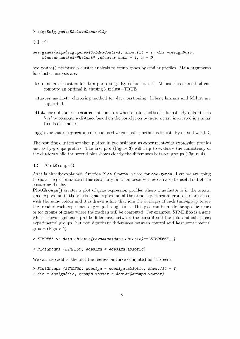
As it is already explained, function Plot Groups is used for see.genes. Here we are goingto show the performance of this secondary function because they can also be useful out of theclustering display.PlotGroups() creates a plot of gene expression profiles where time-factor is in the x-axis,gene expression in the y-axis, gene expression of the same experimental group is representedwith the same colour and it is drawn a line that join the averages of each time-group to seethe trend of each experimental group through time. This plot can be made for specific genesor for groups of genes where the median will be computed. For example, STMDE66 is a genewhich shows significant profile differences between the control and the cold and salt streesexperimental groups, but not significant differences between control and heat experimentalgroups (Figure 5).

> STMDE66 <- data.abiotic[rownames(data.abiotic)=="STMDE66", ]

> PlotGroups (STMDE66, edesign = edesign.abiotic)

We can also add to the plot the regression curve computed for this gene.

> PlotGroups (STMDE66, edesign = edesign.abiotic, show.fit = T,

+ dis = design$dis, groups.vector = design$groups.vector)

8

−1.

00.

01.

02.

0

Cluster 1 ( 36 genes )

expr

essi

on v

alue

Con

trol

_3H

_1C

ontr

ol_3

H_2

Con

trol

_3H

_3C

ontr

ol_9

H_1

Con

trol

_9H

_2C

ontr

ol_9

H_3

Con

trol

_27H

_1C

ontr

ol_2

7H_2

Con

trol

_27H

_3C

old_

3H_1

Col

d_3H

_2C

old_

3H_3

Col

d_9H

_1C

old_

9H_2

Col

d_9H

_3C

old_

27H

_1C

old_

27H

_2C

old_

27H

_3H

eat_

3H_1

Hea

t_3H

_2H

eat_

3H_3

Hea

t_9H

_1H

eat_

9H_2

Hea

t_9H

_3H

eat_

27H

_1H

eat_

27H

_2H

eat_

27H

_3S

alt_

3H_1

Sal

t_3H

_2S

alt_

3H_3

Sal

t_9H

_1S

alt_

9H_2

Sal

t_9H

_3S

alt_

27H

_1S

alt_

27H

_2S

alt_

27H

_3

−4

−2

01

2


expr

essi

on v

alue

Con

trol

_3H

_1C

ontr

ol_3

H_2

Con

trol

_3H

_3C

ontr

ol_9

H_1

Con

trol

_9H

_2C

ontr

ol_9

H_3

Con

trol

_27H

_1C

ontr

ol_2

7H_2

Con

trol

_27H

_3C

old_

3H_1

Col

d_3H

_2C

old_

3H_3

Col

d_9H

_1C

old_

9H_2

Col

d_9H

_3C

old_

27H

_1C

old_

27H

_2C

old_

27H

_3H

eat_

3H_1

Hea

t_3H

_2H

eat_

3H_3

Hea

t_9H

_1H

eat_

9H_2

Hea

t_9H

_3H

eat_

27H

_1H

eat_

27H

_2H

eat_

27H

_3S

alt_

3H_1

Sal

t_3H

_2S

alt_

3H_3

Sal

t_9H

_1S

alt_

9H_2

Sal

t_9H

_3S

alt_

27H

_1S

alt_

27H

_2S

alt_

27H

_3

−0.

50.

51.

5


expr

essi

on v

alue

Con

trol

_3H

_1C

ontr

ol_3

H_2

Con

trol

_3H

_3C

ontr

ol_9

H_1

Con

trol

_9H

_2C

ontr

ol_9

H_3

Con

trol

_27H

_1C

ontr

ol_2

7H_2

Con

trol

_27H

_3C

old_

3H_1

Col

d_3H

_2C

old_

3H_3

Col

d_9H

_1C

old_

9H_2

Col

d_9H

_3C

old_

27H

_1C

old_

27H

_2C

old_

27H

_3H

eat_

3H_1

Hea

t_3H

_2H

eat_

3H_3

Hea

t_9H

_1H

eat_

9H_2

Hea

t_9H

_3H

eat_

27H

_1H

eat_

27H

_2H

eat_

27H

_3S

alt_

3H_1

Sal

t_3H

_2S

alt_

3H_3

Sal

t_9H

_1S

alt_

9H_2

Sal

t_9H

_3S

alt_

27H

_1S

alt_

27H

_2S

alt_

27H

_3

−4

−2

01

2


expr

essi

on v

alue

Con

trol

_3H

_1C

ontr

ol_3

H_2

Con

trol

_3H

_3C

ontr

ol_9

H_1

Con

trol

_9H

_2C

ontr

ol_9

H_3

Con

trol

_27H

_1C

ontr

ol_2

7H_2

Con

trol

_27H

_3C

old_

3H_1

Col

d_3H

_2C

old_

3H_3

Col

d_9H

_1C

old_

9H_2

Col

d_9H

_3C

old_

27H

_1C

old_

27H

_2C

old_

27H

_3H

eat_

3H_1

Hea

t_3H

_2H

eat_

3H_3

Hea

t_9H

_1H

eat_

9H_2

Hea

t_9H

_3H

eat_

27H

_1H

eat_

27H

_2H

eat_

27H

_3S

alt_

3H_1

Sal

t_3H

_2S

alt_

3H_3

Sal

t_9H

_1S

alt_

9H_2

Sal

t_9H

_3S

alt_

27H

_1S

alt_

27H

_2S

alt_

27H

_3

−2

01

23


expr

essi

on v

alue

Con

trol

_3H

_1C

ontr

ol_3

H_2

Con

trol

_3H

_3C

ontr

ol_9

H_1

Con

trol

_9H

_2C

ontr

ol_9

H_3

Con

trol

_27H

_1C

ontr

ol_2

7H_2

Con

trol

_27H

_3C

old_

3H_1

Col

d_3H

_2C

old_

3H_3

Col

d_9H

_1C

old_

9H_2

Col

d_9H

_3C

old_

27H

_1C

old_

27H

_2C

old_

27H

_3H

eat_

3H_1

Hea

t_3H

_2H

eat_

3H_3

Hea

t_9H

_1H

eat_

9H_2

Hea

t_9H

_3H

eat_

27H

_1H

eat_

27H

_2H

eat_

27H

_3S

alt_

3H_1

Sal

t_3H

_2S

alt_

3H_3

Sal

t_9H

_1S

alt_

9H_2

Sal

t_9H

_3S

alt_

27H

_1S

alt_

27H

_2S

alt_

27H

_3

−3

−1

01

2


expr

essi

on v

alue

Con

trol

_3H

_1C

ontr

ol_3

H_2

Con

trol

_3H

_3C

ontr

ol_9

H_1

Con

trol

_9H

_2C

ontr

ol_9

H_3

Con

trol

_27H

_1C

ontr

ol_2

7H_2

Con

trol

_27H

_3C

old_

3H_1

Col

d_3H

_2C

old_

3H_3

Col

d_9H

_1C

old_

9H_2

Col

d_9H

_3C

old_

27H

_1C

old_

27H

_2C

old_

27H

_3H

eat_

3H_1

Hea

t_3H

_2H

eat_

3H_3

Hea

t_9H

_1H

eat_

9H_2

Hea

t_9H

_3H

eat_

27H

_1H

eat_

27H

_2H

eat_

27H

_3S

alt_

3H_1

Sal

t_3H

_2S

alt_

3H_3

Sal

t_9H

_1S

alt_

9H_2

Sal

t_9H

_3S

alt_

27H

_1S

alt_

27H

_2S

alt_

27H

_3

−3

−2

−1

01


expr

essi

on v

alue

Con

trol

_3H

_1C

ontr

ol_3

H_2

Con

trol

_3H

_3C

ontr

ol_9

H_1

Con

trol

_9H

_2C

ontr

ol_9

H_3

Con

trol

_27H

_1C

ontr

ol_2

7H_2

Con

trol

_27H

_3C

old_

3H_1

Col

d_3H

_2C

old_

3H_3

Col

d_9H

_1C

old_

9H_2

Col

d_9H

_3C

old_

27H

_1C

old_

27H

_2C

old_

27H

_3H

eat_

3H_1

Hea

t_3H

_2H

eat_

3H_3

Hea

t_9H

_1H

eat_

9H_2

Hea

t_9H

_3H

eat_

27H

_1H

eat_

27H

_2H

eat_

27H

_3S

alt_

3H_1

Sal

t_3H

_2S

alt_

3H_3

Sal

t_9H

_1S

alt_

9H_2

Sal

t_9H

_3S

alt_

27H

_1S

alt_

27H

_2S

alt_

27H

_3

−6

−2

02


expr

essi

on v

alue

Con

trol

_3H

_1C

ontr

ol_3

H_2

Con

trol

_3H

_3C

ontr

ol_9

H_1

Con

trol

_9H

_2C

ontr

ol_9

H_3

Con

trol

_27H

_1C

ontr

ol_2

7H_2

Con

trol

_27H

_3C

old_

3H_1

Col

d_3H

_2C

old_

3H_3

Col

d_9H

_1C

old_

9H_2

Col

d_9H

_3C

old_

27H

_1C

old_

27H

_2C

old_

27H

_3H

eat_

3H_1

Hea

t_3H

_2H

eat_

3H_3

Hea

t_9H

_1H

eat_

9H_2

Hea

t_9H

_3H

eat_

27H

_1H

eat_

27H

_2H

eat_

27H

_3S

alt_

3H_1

Sal

t_3H

_2S

alt_

3H_3

Sal

t_9H

_1S

alt_

9H_2

Sal

t_9H

_3S

alt_

27H

_1S

alt_

27H

_2S

alt_

27H

_3

−2.

0−

1.0

0.0

1.0


expr

essi

on v

alue

Con

trol

_3H

_1C

ontr

ol_3

H_2

Con

trol

_3H

_3C

ontr

ol_9

H_1

Con

trol

_9H

_2C

ontr

ol_9

H_3

Con

trol

_27H

_1C

ontr

ol_2

7H_2

Con

trol

_27H

_3C

old_

3H_1

Col

d_3H

_2C

old_

3H_3

Col

d_9H

_1C

old_

9H_2

Col

d_9H

_3C

old_

27H

_1C

old_

27H

_2C

old_

27H

_3H

eat_

3H_1

Hea

t_3H

_2H

eat_

3H_3

Hea

t_9H

_1H

eat_

9H_2

Hea

t_9H

_3H

eat_

27H

_1H

eat_

27H

_2H

eat_

27H

_3S

alt_

3H_1

Sal

t_3H

_2S

alt_

3H_3

Sal

t_9H

_1S

alt_

9H_2

Sal

t_9H

_3S

alt_

27H

_1S

alt_

27H

_2S

alt_

27H

_3

Figure 3: Cluster Analysis ColdvsControl significant genes

9

●

●●

●

●

●

●

●●

●

●

●

●

●

●

●

●

●

●

●

●

●

●

●

●

●

●

●

●

●

●●●

●

●

●

−0.

20.

20.

6

Cluster 1

Median profile of 36 genestime

Exp

ress

ion

valu

e

3 9 27

ControlColdHeatSalt

●

●

●

●

●●

●

●

●

●

●

●

●

●

●

●

●

●

●

●

●

●

●●

●

●

●

●

●

●

●

●●

●●

●

−0.

8−

0.4

0.0

Cluster 2


Exp

ress

ion

valu

e

3 9 27

ControlColdHeatSalt

●

●

●

●

●

●

●

●●

●

●●

●

●

●

●

●

●

●

●

●

●

●

●

●

●

●

●

●

●

●

●● ●

●

●

0.0

0.4

0.8

Cluster 3


Exp

ress

ion

valu

e

3 9 27

ControlColdHeatSalt

●

●

●●●

●

●

●

●

●●

●

●

●

●

●

●●

●

●

●

●

●

●

●

●

●

●

●

●

●

●

●

●

●

●

−0.

20.

20.

6

Cluster 4


Exp

ress

ion

valu

e

3 9 27

ControlColdHeatSalt

●

●

●

●●

●

●

●

●

●

●●

●

●

●

●●

●

●

●

●

●

●

●

●

●

●

●

●

●

●

●

●

●

●

●

−0.

6−

0.2

0.2

0.6

Cluster 5


Exp

ress

ion

valu

e

3 9 27

ControlColdHeatSalt

●●

●

●

●

● ●

●

●

●

●

●

●●

●

●●

●

●

●

●

●

●

●

●

●

●

●●

●●●

●

●●●

−0.

8−

0.2

0.2

Cluster 6


Exp

ress

ion

valu

e

3 9 27

ControlColdHeatSalt

●

●

●

●

●

●

●

●

●

●

●

●

●

●

●

●

●

●

●

●

●

●

●

●

●

●●

●

●

●

●

●

●●●●

−1.

0−

0.4

0.0

Cluster 7


Exp

ress

ion

valu

e

3 9 27

ControlColdHeatSalt

●

●●

●

●

●

●

●●

●

●●

●

●

●

●

●

●

●

●

●

●

●

●

●

●

●

●

●

●●

●

●

●

●

●

−0.

8−

0.4

0.0

Cluster 8


Exp

ress

ion

valu

e

3 9 27

ControlColdHeatSalt

●●

●

●

●

●

●

●

●

●

●

●

●

●

●

●

●

●

●

●●

●

●

●

●

●

●

●

●

●●●●

●

●

●

−0.

40.

00.

20.

4

Cluster 9


Exp

ress

ion

valu

e

3 9 27

ControlColdHeatSalt

Figure 4: Expression Profiles ColdvsControl significant genes

10

●

●●

●

●● ●

●●

●

●

●

●●

●

●

●

●

●

●

●

●

●

●

●

●

●

●

●

●

●

●

●

●

●

●

−2.

0−

1.5

−1.

0−

0.5

0.0

0.5

STMDE66Time

Exp

ress

ion

valu

e

3 9 27

ControlColdHeatSalt

●

●●

●

●● ●

●●

●

●

●

●●

●

●

●

●

●

●

●

●

●

●

●

●

●

●

●

●

●

●

●

●

●

●

−2.

0−

1.5

−1.

0−

0.5

0.0

0.5

STMDE66Time

Exp

ress

ion

valu

e

3 9 27

ControlColdHeatSalt

(a) (b)

Figure 5: PlotGroups of gene STMDE66 without and with display or regression curves

4.4 PlotProfiles()

This secondary function creates a plot of gene expression profiles where x-axis represents theorder of the columns of the data matrix and the y-axis represents the gene expression. Whena group of genes if plotted they will be represented with different colours. The main goal ofthis graph is to check the homogeneity of the clusters.

5 Other designs

5.1 Single Series Time Course

The use of maSigPro in Single Series Time Course experiment is straightforward. Makea edesign object with just one group column containing all 1s and proceed as describedabove. Note that when using the get.siggenes() funcion the options ”all” and ”groups” ofthe argument vars will return the same result. You can use option ”each” to analyze the typeof responses present in the significant genes: significant genes at the ”intercept” term will havea significant expression value at the starting time; genes associated to the variable ”Time”will have a significant linear component, which can be induction or repression depending onthe sign of their coefficient; genes associated to the variable ”Time2” will show a change inthe linear response that might be indicating transitory or saturation reponses, etc...Here follows an example of a Single Series analysis.

## make a single series edesign

> Time <- rep(c(1,5,10,24), each = 3)

> Replicates <- rep(c(1:4), each = 3)

> Group <- rep(1,12)

11

> ss.edesign <- cbind(Time,Replicates,Group)

> rownames(ss.edesign) <- paste("Array", c(1:12), sep = "")

## Create data set

> ss.GENE <- function(n, r, var11 = 0.01, var12 = 0.02, var13 = 0.02,

var14 = 0.02, a1 = 0, a2 = 0, a3 = 0, a4 = 0) {

tc.dat <- NULL

for (i in 1:n) {

gene <- c(rnorm(r, a1, var11), rnorm(r, a1, var12),

rnorm(r, a3, var13), rnorm(r, a4, var14))

tc.dat <- rbind(tc.dat, gene)

}

tc.dat }

> flat <-ss.GENE(n = 85, r = 3) # flat

> induc <- ss.GENE(n = 5, r = 3, a1 = 0, a2 = 0.2, a3 = 0.6, a4 = 1) # induction

> sat <- ss.GENE(n = 5, r = 3, a1 = 0, a2 = 1, a3 = 1.1, a4 = 1.2) # saturation

> ord <- ss.GENE(n = 5, r = 3, a1 = -0.8, a2 = -1, a3 = -1.3, a4 =-0.9) # intercept

> ss.DATA <- rbind(flat, induc,sat,ord)

> rownames(ss.DATA) <- paste("feature", c(1:100), sep = "")

> colnames(ss.DATA) <- paste("Array", c(1:12), sep = "")

# run maSigPro

> ss.example <- maSigPro(ss.DATA, ss.edesign, vars="each")

5.2 Common Starting Time

The following example illustrates how to build the edesign matrix when a common 0 time isapplicable to the different experimental groups.

> data(edesignCT)

In this example Array1 and Array2 do not belong to any treatment. They are a commonreference for all groups, values without any treatment at time 0.

12

6 Next Generation-Sequencing series

maSigPro uses lm() function to fit a linear model where statistics for inference use normaldistribution. This is the right treatment when dealing with normal distributed data or bigsamples. However, for non-normal small samples, results can not be correct.The statistical distribution for tag counts data as RNA-Seq data may be Poisson or Binomial.However, the overdispersion of the data suggest the Negative Binomial (NB) can model thesedistributions in a better way. This distribution depends on a θ parameter to model theoverdispersion that is related to the mean(µ) in the following way:

Y ∼ NB(θ), V ar(Y ) = µ+µ2

θ

maSigPro has been adapted to take into account non-normal distribution of the data (Nuedaet al., 2014). New arguments have been added in p.vector function to deal with this typeof data in a proper way:

counts: a logical indicating whether your data are counts. By default is FALSE for mi-croarray treatment.

theta: θ parameter for negative.binomial family. By default θ = 10.

family: the distribution function to be used in the GLM. It must be specified as a func-tion: gaussian(), poisson(), negative.binomial(theta)... If NULL family will be nega-tive.binomial(theta) when counts=TRUE or gaussian() when counts=FALSE.

The recommended analysis to deal with RNA-Seq data is the GLM with negative.binomialfamily. θ must be specified and it can be computed by using available methods as edgeR((Robinson et al., 2010)). The application of maSigPro with several values of θ to the samedatasets did not reveal significant differences in gene selection. Taking this into considerationwe have put by default θ = 10 for being an average value. Moreover we give to the user theoption of applying whatever exponential family to explore other possibilities.Data must be normalized before the application of maSigPro as it is not integrated anynormalized method.NBdata is a subset of a bigger normalized dataset with 2 experimental groups, 6 time-pointsand 3 replicates. Simulation has been done by using a negative binomial distribution withθ = 5 to illustrate this section. The first 20 genes are simulated with changes among time.NBdesign is the design matrix.

> data(NBdata)

> data(NBdesign)

> d <- make.design.matrix(NBdesign)

If we can use maSigPro with theta = 10:

> library(MASS)

> NBp <- p.vector(NBdata, d, counts=TRUE)

> NBt <- T.fit(NBp)

> get<-get.siggenes(NBt, vars="all")

> get$summary

13

●

●●

●●●

●●

● ●●

●●●● ●●

●●●

●

●●●

●

●

●

●

●

●

●

●

●

●

●

●

020

6010

014

0

Cluster 1


aver

age

expr

essi

on v

alue

0 12 24 36 48 60

Group.1Group.2

●●●

●●●

●●●

●●●

●●●

●●●●●●

●

●●

●

●

●

●

●

●

●

●

●

●

●

●

020

6010

014

0

Cluster 2


aver

age

expr

essi

on v

alue

0 12 24 36 48 60

Group.1Group.2

●

●

●

●

●

●

●

●

● ●

●●

●

●

● ●

●

●

●

●

●

●

●●

●

●

● ●

●

●

●

●

●

●●●050

100

150

Cluster 3


aver

age

expr

essi

on v

alue

0 12 24 36 48 60

Group.1Group.2

●

●●

●

●

●

●

●

●

●

●

●

●

●

●

●

●

●

●

●

●

●

●

●

●

●●

●●

●●

●●

●●●050

100

150

Cluster 4


aver

age

expr

essi

on v

alue

0 12 24 36 48 60

Group.1Group.2

Figure 6: Cluster Analysis significant genes

These genes can be grouped in 4 clusters 6:

see.genes(get$sig.genes, k = 4)

If we can use maSigPro with a specific theta, in this case, theta = 5:

> NBp <- p.vector(NBdata, d, counts=TRUE, theta=5)

Also, a specific family, for instance, poisson can be specified. In such case counts and thetaparameters are omitted.

> NBp <- p.vector(NBdata, d, family=poisson() )

Changing this arguments in p.vector is enough. Further functions will take these argumentsfrom a p.vector object.

14

7 Iso-maSigPro: analysis of alternative isoform expression intime course transcriptomics experiments

maSigPro package includes several tools for the analysis of alternative isoform expression intime course transcriptomics experiments. Figure 7 shows the analysis pipeline with functionsinvolved in this analysis.

IsoModel() fits model for DS

getDS() selects significant DSGs and DETs

tableDS() identifies cluster location

of major and minor isoforms

seeDS() clusters DETs

PodiumChange() finds DSGs with major isoform switch

getDSPattern() extracts genes with specific isoform clustering pattern

IsoPlot() shows expression of indicated DGS

Figure 7: ISO-maSigPro pipeline.

For Iso-maSigPro analysis, data must be provided as a transcript-level expression data set,similarly to regular maSigPro. This data.frame must include TranscriptIDs as rownamesand the GeneID of each transcript in the first column. The Iso-maSigPro package does notinclude functions for quantification of isoform expression.The package provides a test dataset for differential splicing analysis named ISOdata. Itconsists of 2782 isoforms (rows) belonging to 1009 genes. The experimental desing is a 2series experiment with 6 time points and three replicates per experimental condition. Firstcolumn of ISOdata contains the name of the gene each isoform belongs to, while the remainingcolumns are the RNA-Seq data samples associated to the experimental conditions.

> data(ISOdata)

> data(ISOdesign)

> dis <- make.design.matrix(ISOdesign)

7.1 IsoModel() and getDS()

First of all IsoModel() function is applied to identify Differentially Spliced Genes (DSGs) andalso Differentially Expressed Transcripts (DETs), which are transcripts of significant DSGsdetected as statistically significant with regular NextmaSigPro. IsoModel() returns a list ofDSGs and all the information about the estimated models of associated isoforms to be used asinput in getDS() function to obtain a selection of DSGs at a preestablished level of goodnessof fit for each model.

> MyIso <- IsoModel(data=ISOdata[,-1], gen=ISOdata[,1], design=dis, counts=TRUE)

15

[1] "2782 transcripts"

[1] "1009 genes"

[1] "fitting gene 100 out of 568"





[1] "fitting isoform 100 out of 241"



[1] "Influence: 17 genes with influential data at slot influ.info."

> Myget <- getDS(MyIso)

[1] "51 DSG selected"

[1] "97 DETs selected"

DSG_distributed_by_number_of_DETs

1 2 3 4 9 10

17 21 1 4 1 1

When applying getDS() function the number of DSGs and DETs are showed by console andalso a table detailing the number of DETs that each selected DSG contains. Names of DSGsand DETs can be showed with:

> Myget$DSG

[1] "Gene239" "Gene1009" "Gene1005" "Gene800" "Gene64" "Gene1003"








[49] "Gene285" "Gene652" "Gene595"

> Myget$DET

[1] "Transcript122" "Transcript125" "Transcript147" "Transcript150"










16















[97] "Transcript2732"

Note that it is possible that a gene called DSG but no significant DET can be found underthe significance level, goodness of fit and multiple testing correction constraints of the regularmaSigPro analysis. Names of such cases can be shown with:

> Myget$List0


7.2 Clustering strategy: seeDS() and tableDS()

The Iso-maSigPro clustering approach identifies groups of DSGs with similar isoform ex-pression patterns, as well as the expression profiles of DETs within DSGs. This strategy isimplemented in two steps corresponding to seeDS() and tableDS() functions.Function seeDS looks for general transcript expression trends analysing DETs and clustersthem into k groups with any of the available maSigPro clustering approaches (cluster.methodinput can be: hclust, kmeans or Mclust, the most used clustering methods). The clusteringcan be applied to only DETs from DSGs (cluster.all=FALSE) or after computing DETsfrom all available genes (cluster.all=TRUE), which is recommended when the interest isto characterize the expression pattern of the whole transcriptomics experiment and not onlyfrom DSGs. Figure 8 shows the clusters obtained for DETs in our example.

> see <- seeDS(Myget, cluster.all=FALSE, k=6)

17

●

●

●

●

●●

●

●

●

●

●

●

●

●

●

●

●

●

●

●●

●

●

●

●

●●

●

●

●

●

●●

●

●

●

1020

3040

Cluster 1

Median profile of 16 Isoformstime

Exp

ress

ion

valu

e

0 2 6 12 18 24

Group1Group2 ●●

●●

●

●

●

●●

●●●

●

●

●

●

●

●

●●● ●●

●●●

●

●

●

●

●

●● ●

●●0

510

1520

Cluster 2


Exp

ress

ion

valu

e

0 2 6 12 18 24

Group1Group2

●

●

● ●●●

●

●●

●●●

●

●●

●

●

●

●

●

● ●●

●

●

●

●

●●

●

●●●

●

●

●

24

68

12

Cluster 3


Exp

ress

ion

valu

e

0 2 6 12 18 24

Group1Group2

●

●● ●

●

●

●

●● ●●●

●●● ●

●●

●●

●

●

●

●

●

●

●

●

●

●

●

●

●

●

●

●

510

1520

25Cluster 4


Exp

ress

ion

valu

e

0 2 6 12 18 24

Group1Group2

●●● ●●●

●●●

●●●●●● ●●●

●●●

●●●●●

●

●

●

●

●

●

●

●

●●

02

46

812

Cluster 5


Exp

ress

ion

valu

e

0 2 6 12 18 24

Group1Group2

●

●

●

●

●

●

●

●

●

●

●

●

●

●●

●

●

●

●

●

●●

●

●

●●

●

●

●●

●

●● ●

●

●

4060

80

Cluster 6


Exp

ress

ion

valu

e

0 2 6 12 18 24

Group1Group2

Figure 8: Cluster Analysis Differentially Expressed Transcripts (DETs)

18

Next, the tableDS() function takes DSGs with 2 or more DETs to identify the time-courseAlternative Splicing events. To do this, each DET is labeled as major isoform (defined as themost expressed isoform across conditions) or minor isoform and for each DSG the clusterswhere their major and minor DET(s) belong are identified. This information is used tocompute a classification table that indicates the distribution of DETs of DSG across differentclusters.

> table <- tableDS(see)

> table$IsoTable

Cluster.minor

Cluster.Mayor 1 1&5 2 3 3&4 4 5

1 0 1 1 1 0 3 1

2 1 0 0 0 0 0 0

3 0 0 1 0 1 2 0

4 0 0 0 1 2 4 2

5 0 0 0 0 0 0 2

6 0 0 0 2 0 1 2

By comparing the classification table with the cluster profiles, the user can readily identifygenes with strong or subtle expression differences among their set of isoforms. For instance,in Figure 8 it is observed that cluster 1 and 4 have diferent trends and IsoTable object showsthere are 3 genes with major isoform in cluster 1 and minor isoform(s) in cluster 4. Thenames of these genes can be obtained with the getDSPatterns() function:

> getDSPatterns(table, 1, 4)

[1] "Gene1002" "Gene1003" "Gene1004"

The gene selection can be plotted with IsoPlot() function (see example in Figure 9).

7.3 PodiumChange()

Alternatively, PodiumChange() function extracts from the data those DSGs that undergoa switch of their most expressed isoform during the time course. PodiumChange() can beapplied taking into consideration only the DETs (only.sig.iso=TRUE)or considering all theisoforms of DSGs. This last option is interesting when the DSG has only one isoform calledas DET. The function takes as input the result of getDS() and returns a list of genes withpodium changes. The function can detect changes at any time point (eventual changes),for an indicated experimental condition or at specific subranges of time and experimentalconditions.

> PC<-PodiumChange(Myget, only.sig.iso=TRUE, comparison="specific",

+ group.name="Group2", time.points=c(18,24))

> PC$L

[1] "Gene239" "Gene1008" "Gene1005"

Again, the gene selection can be plotted with IsoPlot() function (see example in Figure 9).

19

05

1015

20

Group1

Time

Exp

ress

ion

valu

e

0 2 6 12 18 24

●

●

●

●

●

●

●

●

●

●

●●

●

●

●

●

●

●

●●

●

●●

●

●

●

●

●

●

●

●

●

●

●

●

●

●●● ●●● ●●● ●●● ●●● ●●●

●

●● ●●

● ●

●●

●●

●

●●●

●●

●

●●● ●●

●

●

●

●

●●● ●

●

●

●●

●

●●●

●●

●

●

●● ●

●

●

●●

●

●

●

●●●●

●●●

●

●

●

●

●● ●●

●

●●

●

Group2

Time

Exp

ress

ion

valu

e

0 2 6 12 18 24

●

●

●

●●

●

●

●●

●

●

●

●

●

●

●

●

●

●

●

●

●●

●

●

●

●●●

●

●

●

●

●

●

●

●●● ●●● ●●●

●●

● ●●

●

●

●

●

●

●●●●

●

●

●

●

●●

●

●●● ●●●●●●

●

●

●

●●

●

●●

●

●●

● ●●

●●●● ●

●

●●●●

●

●

●

●●●●●

●

●

●●

●●

●

●●

●

●●

●

●

●●

●

●

●

Transcript2633Transcript2634Transcript2635Transcript2636Transcript2637Transcript2638Transcript2639

Gene1005

Figure 9: IsoPlot() example. Gene1005 detected as podium-change gene.

7.4 IsoPlot()

This function provides gene-level plots of the expression profiles of all transcripts in the inputvector of gene names. Optionally, the user can choose visualizing all transcripts or only DETsof the selected genes. Typically, IsoPlot() can be used to inspect specific genes identified bythe PodiumChange() or the tableDS() functions. Figure 9 shows the IsoPlot() of Gene1005detected as podium-change gene.

> IsoPlot(Myget,"Gene1005",only.sig.iso=FALSE,cex.main=2,cex.legend=1)

20

References

Y. Benjamini and Y. Hochberg. Controlling the false discovery rate: a practical and powerfulapproach to multiple testing. Journal of the Royal Statistical Society Series B, 57:289–300,1995. URL http://wwwtigr.org/tdb/potato/index.shtml.

A. Conesa, M. Nueda, A. Ferrer, and M. Talon. maSigPro: a method to identify signif-icantly differential expression profiles in time-course microarray experiments. Bioinfor-matics, 22(9):1096–1102, 2006. URL http://bioinformatics.oupjournals.org/cgi/

content/abstract/22/9/1096.

M. Nueda, S. Tarazona, and A. Conesa. Next maSigPro: updating maSigPro bioconductorpackage for RNA-seq time series. Bioinformatics, 30(18):2598–2602, 2014. URL http:

//bioinformatics.oxfordjournals.org/content/30/18/2598.

W. Rensink, S. Iobst, A. Hart, S. Stegalkina, J. Liu, and C. Buell. Gene expression profilingof potato responses to cold, heat and salt stress. Funct Integr Genomics, 5(4):201–207,2005. URL http://wwwtigr.org/tdb/potato/index.shtml.

M. Robinson, D. McCarthy, and G. Smyth. edgeR: a Bioconductor package for differentialexpres-sion analysis. Bioinformatics, 26:139–140, 2010.

21

http://wwwtigr.org/tdb/potato/index.shtml

http://bioinformatics.oupjournals.org/cgi/content/abstract/22/9/1096

http://bioinformatics.oupjournals.org/cgi/content/abstract/22/9/1096

http://bioinformatics.oxfordjournals.org/content/30/18/2598

http://bioinformatics.oxfordjournals.org/content/30/18/2598

http://wwwtigr.org/tdb/potato/index.shtml

masigpro user’s guide - bioconductorbioconductor.org/.../inst/doc/masigprousersguide.pdfmasigpro...

Documents