mas435algebraictopology 2012–13 partb:semester2cheng.staff.shef.ac.uk/mas435/algtop-partb.pdf ·...
TRANSCRIPT

MAS435 Algebraic Topology
2012–13
Part B: Semester 2
Dr E Cheng
School of Mathematics and Statistics, University of Sheffield
E-mail: [email protected]
http://cheng.staff.shef.ac.uk/mas435/
Notes taken by Alex Corner
Contents
1 Chain complexes and homology 3
1.1 Chain complexes . . . . . . . . . . . . . . . . . . . . . . . . . . . 3
1.2 Homology . . . . . . . . . . . . . . . . . . . . . . . . . . . . . . . 4
1.3 Products of abelian groups . . . . . . . . . . . . . . . . . . . . . 4
1.4 Free abelian groups . . . . . . . . . . . . . . . . . . . . . . . . . . 5
1.5 Maps between chain complexes . . . . . . . . . . . . . . . . . . . 6
2 Low-dimensional cell-complexes 7
2.1 Low-dimensional examples . . . . . . . . . . . . . . . . . . . . . . 7
2.2 Simplices . . . . . . . . . . . . . . . . . . . . . . . . . . . . . . . 9
3 Singular homology and homotopy invariants 11
3.1 Reduced homology . . . . . . . . . . . . . . . . . . . . . . . . . . 11
3.2 Homotopy invariance . . . . . . . . . . . . . . . . . . . . . . . . . 12
4 Abelian groups and abelianisation 13
4.1 Abelianisation . . . . . . . . . . . . . . . . . . . . . . . . . . . . . 13
4.2 Finitely-generated abelian groups . . . . . . . . . . . . . . . . . . 14
5 What happened to van Kampen’s Theorem? 15
6 Quotients and relative homology 20
6.1 Mayer-Vietoris Sequence . . . . . . . . . . . . . . . . . . . . . . . 23
7 Axioms for homology 24
CONTENTS 2
8 Further remarks 25
8.1 Moore spaces . . . . . . . . . . . . . . . . . . . . . . . . . . . . . 25
8.2 Wedge sums . . . . . . . . . . . . . . . . . . . . . . . . . . . . . . 25
8.3 Suspension . . . . . . . . . . . . . . . . . . . . . . . . . . . . . . 26
Introduction
We have seen that Algebraic Topology is about studying topological spaces using
algebra. In the first part of the course the algebra we used was group theory.
We saw how to study a topological space X via its “fundamental group” π1X
which helped us some features of spaces but not others. The main limitation
was that the fundamental group is constructed from loops in a space, and cannot
detect higher-dimensional features.
The higher-dimensional versions of the fundamental group are constructed from
higher-dimensional loops. That is, where a loop in X is a map
S1 −→ X
a higher-dimensional loop is a map
Sn −→ X
for higher values of n; these loops form a group called the nth homotopy group
πnX . The trouble with this approach is that it is very difficult to compute.
That is why we turn to homology instead. It is easier to compute than higher
homotopy groups, but as a trade-off, it is less sensitive. In fact in this course
we will not do a lot of higher-dimensional calculation.
The idea of homology is to produce, from a space X , an Abelian group Hn(X)
called its nth homology group. In fact, we proceed in two steps:
space chain complex homology groups
A “chain complex” is a well-behaved sequence of abelian groups and homomor-
phisms, as we’ll see. This means that homology can be used to study a wide
range of things, not just spaces, as long as some sort of chain complex can be
obtained from those things. So the first step above immediately gets us into
algebra, and the second step is all within the world of algebra. The study of
chain complexes and their associated homology group is called homological
1 Chain complexes and homology 3
algebra and can be thought of as a particularly structured part of the world of
abelian groups.
For the first step, it helps if we know how our how space is built up dimension
by dimension from “cells”, that is, some form of disk/ball. Homology will then
1. find the places where we could have attached disks, and
2. compare it with the places where we actually did attach disks.
Formally, this is done by taking a quotient group. This quotient group measures
how “holey” the space is, because it measures the “holes” that were not filled
in by disks.
The slogan of homology is cycles mod boundaries. A “cycle” is the algebraic
version of a “hole”. A “boundary” is a hole that we filled in with a disk—it has
now become the boundary of a disk.
1 Chain complexes and homology
We need to start by looking at the algebraic objects we’ll be using: chain com-
plexes of abelian groups. All the groups in this part of the course are abelian,
which makes a lot of things easier.
1.1 Chain complexes
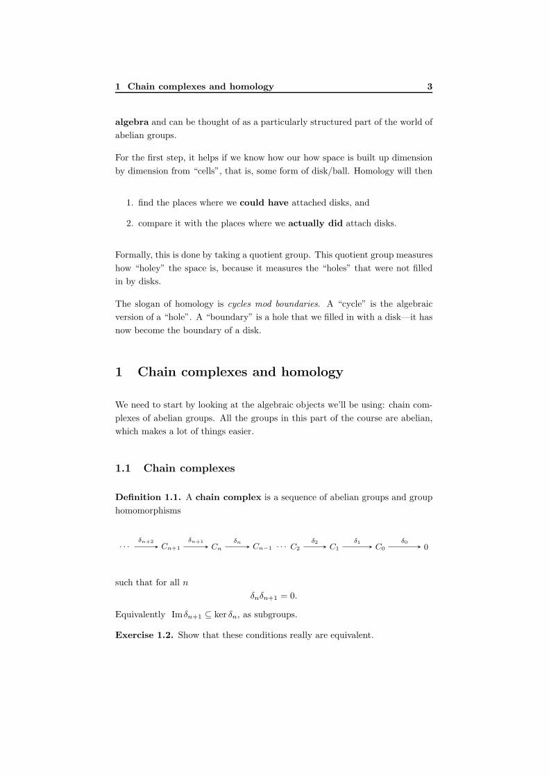
Definition 1.1. A chain complex is a sequence of abelian groups and group
homomorphisms
· · · Cn+1 Cn Cn−1 · · · C2 C1 C0 0δn+2 δn+1 δn δ2 δ1 δ0
such that for all n
δnδn+1 = 0.
Equivalently Imδn+1 ⊆ ker δn, as subgroups.
Exercise 1.2. Show that these conditions really are equivalent.
1.2 Homology 4
Terminology The maps δ are called boundary maps or differentials and
a chain complex such as the one above may be labelled as C• or sometimes just
C. The elements of Imδn+1 are then called boundaries and those of ker δn
are called cycles.
Definition 1.3. If Imδn+1 = ker δn for all n then the chain complex is called
an exact sequence.
Another slogan is that homology measures the failure of a chain complex to be
exact, as we will now see from the definition.
1.2 Homology
Definition 1.4. The nth homology group of a chain complex C is defined to
be the quotient group
Hn(C) = ker δn/ Imδn+1.
Exercise 1.5. What are two different ways of thinking of the elements of this
group? Do we have to worry about whether or not this is a normal subgroup?
Thinking of elements of Hn(C) as equivalence classes of cycles, we call them ho-
mology classes. Two equivalent cycles are then called homologous ; the condition
for being homologous is as follows:
f ∼ g ⇔ f − g ∈ Imδn+1.
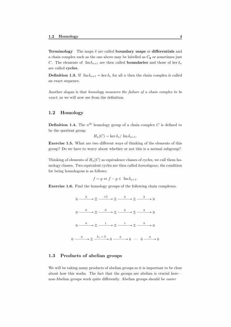
Exercise 1.6. Find the homology groups of the following chain complexes.
0 Z Z Z 00 ×2 0 0
0 Z Z Z 00 0 0 0
0 Z Z Z 00 1 1 0
0 Z 0 0 · · · 0 00 δn = 0 0 0
1.3 Products of abelian groups
We will be taking many products of abelian groups so it is important to be clear
about how this works. The fact that the groups are abelian is crucial here—
non-Abelian groups work quite differently. Abelian groups should be easier
1.4 Free abelian groups 5
Recall that given two abelian groups A and B we can form their direct product
A×B, elements of which are pairs (a, b) where a ∈ A and b ∈ B. This is again
an abelian group, inheriting its group operation from A and B: (a, b)+(a′, b′) =
(a + a′, b + b′). As A × B is abelian here, the group operation will be written
additively.
Exercise 1.7. Show that this really is abelian.
Similarly, recall the direct sum of A and B, the abelian group A⊕B. This has
elements a⊕ b where again a ∈ A and b ∈ B. The group operation is given by
(a⊕ b)+(a′⊕ b′) = (a+a′)⊕ (b+ b′), again using the group operations of A and
B. There is then an obvious isomorphism of abelian groups A×B ∼= A⊕B.
Exercise 1.8. Construct this isomorphism. You should construct the map,
show it’s a group homomorphism, and show it’s an isomorphism.
Remark 1.9. Note that A⊕B is the coproduct of A and B in the category Ab
of abelian groups and group homomorphisms. This is not the case for arbitrary
groups in the category Gp of groups and group homomorphisms. In Gp the
coproduct of groups G and H is the free product G ∗H . However in both Ab
and in Gp the product of two groups is the same, i.e. it is the direct product.
1.4 Free abelian groups
The free abelian group on one generator is isomorphic to Z. For two generators
it is isomorphic to Z ⊕ Z. Carrying on in this way, for k generators, it is
isomorphic to Z⊕k. If we write the generators/basis elements as e1, . . . , ek then
a general element of Z⊕k is Σki=1λiei, where λi ∈ Z. All of our chain complexes
will involve free abelian groups generated by cells of the space.
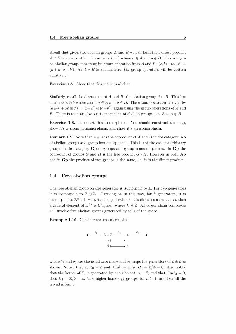
Example 1.10. Consider the chain complex
0 Z⊕ Z Z 0
α
β
a
a
δ2 δ1 δ0
where δ2 and δ0 are the usual zero maps and δ1 maps the generators of Z⊕Z as
shown. Notice that ker δ0 = Z and Imδ1 = Z, so H0 = Z/Z = 0. Also notice
that the kernel of δ1 is generated by one element, α − β, and that Imδ2 = 0,
thus H1 = Z/0 = Z. The higher homology groups, for n ≥ 2, are then all the
trivial group 0.

1.5 Maps between chain complexes 6
1.5 Maps between chain complexes
Just as there are maps between abelian groups, we can define maps between
chain complexes.
Definition 1.11. A chain map of chain complexes f : A→ B is a collection of
group homomorphisms fn : An → Bn, for all n, such that the following diagram
commutes.
An An−1
Bn Bn−1
δn
fn fn−1
ǫn
Proposition 1.12. A chain map as above induces a group homomorphism
Hn(f) : Hn(A) → Hn(B), for all n.
Proof. Given the chain map f , as above, we need to define a group homo-
morphism Hn(f) : ker δn/ Imδn+1 → ker ǫn/ Im ǫn+1. Given a ∈ ker δn, is
fn(a) ∈ ker ǫn? Yes, by commutativity of the following diagram.
An+1 An An−1
Bn+1 Bn Bn−1
δn+1
fn+1
δn
fn fn−1
ǫn+1 ǫn
That is to say fn−1δn(a) = fn−1(0) = 0 = ǫnfn(a). So we have a map ker δn →
ker ǫn. Now consider an element a ∈ Imδn+1, so a = δn+1(x) say. We need that
fn(a) ∈ Im ǫn+1. However fn(a) = fnδn+1(x) = ǫn+1fn+1(x) by commutativity
of the diagram. Thus fn(a) ∈ Im ǫn+1. Thus the map ker δn → ker ǫn restricts
to a map Imδn+1 → Im ǫn+1 and so we can construct the map Hn(A) →
Hn(B), as required.
Note that for each n, Hn is a functor from the category ChCpx of chain com-
plexes and chain maps into the category Ab of abelian groups and group ho-
momorphisms. The above proposition gives us the action on morphisms.
Exercise 1.13. Check that this really is a functor.

2 Low-dimensional cell-complexes 7
2 Low-dimensional cell-complexes
Now that we’ve seen how to produce homology groups from a chain complex,
we need to see how to produce a chain complex from a topological space. There
are various different ways of doing this, like different “recipes”. They do not
all produce the same answer, but the clever part is that the resulting homology
groups are the same. This is a profound and amazing result that is beyond the
scope of this course.
One way of producing a chain complex from a space is to start with a cell
complex structure on the space. We’ve already seen that you can build the
same space using different cell complex structures, but again, this doesn’t matter
because you’ll get the same homology groups at the end, no matter what cell
complex structure you choose.
2.1 Low-dimensional examples
Definition 2.1. Starting from a cell complex, we produce a chain complex C
with:
Cn = the free abelian group generated by the n-cells of our cell complex,
δn = boundaries, considering orientation in a way that we’ll see.
Actually the definition of “orientation” is quite complicated in high dimensions,
so we’ll just do some low dimensional examples.
• For 1-cells the boundary is “head − tail”.
• For 2-cells the boundary is the sum of all the boundary 1-cells, taking
orientation into account (a bit like when we did van Kampen’s theorem
before, and were reading off the boundary of a cell). So if a 1-cell is
pointing “backwards” it gets a minus sign.
Example 2.2. A possible cell complex for the Torus is the following.
a
b
b
aα
x
xx
x

2.1 Low-dimensional examples 8
This has
• one 0-cell x, so C0 has one generator x,
• two 1-cells a and b, so C1 has two generators a, b,
• one 2-cell α, so C2 has one generator α, and
• no higher dimensional cells than these, so Cn is 0 for higher n.
Recall that the free abelian group on one generator is isomorphic to Z, and with
two generators it is isomorphic to Z⊕ Z.
The boundary of both a and b is “head − tail” i.e. x− x = 0. The boundary of
α is a+ b− a− b = 0.
The associated chain complex is then:
· · · 0 Z Z⊕ Z Z 0
α a
b
0 0
0
0 0 0 0
Exercise 2.3. Below are possible cell complexes for the circle S1, the sphere
S2, the Klein bottle and the real projective plane RP 2. Find the associated
chain complexes and work out the homology.
a
x
x
S1
a
a
αx y
S2
a
b
b
aα
x
xx
x
Klein bottle
a
a
αx x
RP 2
Exercise 2.4. Try some different cell complex structures for the same spaces
and make sure you get the same homology groups. This is a useful way of
checking your answers.
To prove that we get the same homology for different cell structures on the same
space, it is easier to use singular homology, which is more general.
2.2 Simplices 9
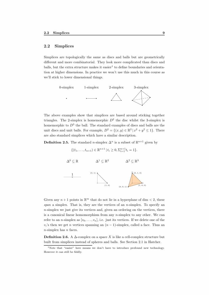
2.2 Simplices
Simplices are topologically the same as discs and balls but are geometrically
different and more combinatorial. They look more complicated than discs and
balls, but the extra structure makes it easier1 to define boundaries and orienta-
tion at higher dimensions. In practice we won’t use this much in this course as
we’ll stick to lower dimensional things.
0-simplex 1-simplex 2-simplex 3-simplex
The above examples show that simplices are based around sticking together
triangles. The 2-simplex is homemorphic D2 the disc whilst the 3-simplex is
homemorphic to D3 the ball. The standard examples of discs and balls are the
unit discs and unit balls. For example, D2 = {(x, y) ∈ R2 |x2 + y2 ≤ 1}. There
are also standard simplices which have a similar description.
Definition 2.5. The standard n-simplex ∆n is a subset of Rn+1 given by
{(t1, . . . , tn+1) ∈ Rn+1 | ti ≥ 0,Σn+1i=1 ti = 1}.
∆0 ⊆ R ∆1 ⊆ R2 ∆2 ⊆ R3
1(0, 1)
(1, 0) (1, 0, 0)
(0, 1, 0)
(0, 0, 1)
Given any n+ 1 points in Rm that do not lie in a hyperplane of dim < 2, these
span a simplex. That is, they are the vertices of an n-simplex. To specify an
n-simplex we just give its vertices and, given an ordering on the vertices, there
is a canonical linear homomorphism from any n-simplex to any other. We can
refer to an n-simplex as [v0, . . . , vn], i.e. just its vertices. If we delete one of the
vi’s then we get n vertices spanning an (n− 1)-simplex, called a face. Thus an
n-simplex has n faces.
Definition 2.6. A ∆-complex on a space X is like a cell-complex structure but
built from simplices instead of spheres and balls. See Section 2.1 in Hatcher.
1Note that “easier” here means we don’t have to introduce profound new technology.
However it can still be fiddly.
2.2 Simplices 10
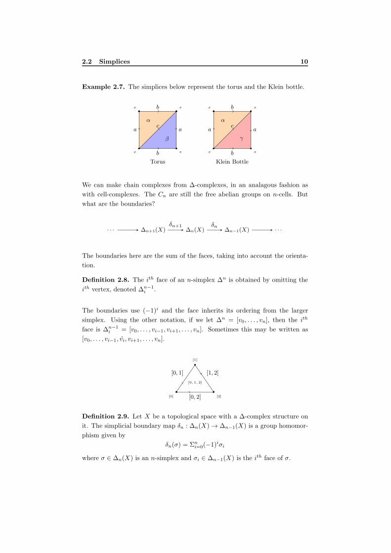
Example 2.7. The simplices below represent the torus and the Klein bottle.
a
b
b
ac
α
β
Torus
x
xx
x
a
b
b
ac
α
γ
Klein Bottle
x
xx
x
We can make chain complexes from ∆-complexes, in an analagous fashion as
with cell-complexes. The Cn are still the free abelian groups on n-cells. But
what are the boundaries?
· · · ∆n+1(X) ∆n(X) ∆n−1(X) · · ·δn+1 δn
The boundaries here are the sum of the faces, taking into account the orienta-
tion.
Definition 2.8. The ith face of an n-simplex ∆n is obtained by omitting the
ith vertex, denoted ∆n−1i .
The boundaries use (−1)i and the face inherits its ordering from the larger
simplex. Using the other notation, if we let ∆n = [v0, . . . , vn], then the ith
face is ∆n−1i = [v0, . . . , vi−1, vi+1, . . . , vn]. Sometimes this may be written as
[v0, . . . , vi−1, vi, vi+1, . . . , vn].
[0] [2]
[1]
[0, 1, 2]
[0, 1]
[0, 2]
[1, 2]
Definition 2.9. Let X be a topological space with a ∆-complex structure on
it. The simplicial boundary map δn : ∆n(X) → ∆n−1(X) is a group homomor-
phism given by
δn(σ) = Σni=0(−1)iσi
where σ ∈ ∆n(X) is an n-simplex and σi ∈ ∆n−1(X) is the ith face of σ.

3 Singular homology and homotopy invariants 11
3 Singular homology and homotopy invariants
The idea of singular homology is that we don’t have to start with a specific ∆-
complex structure. Recall that a path in a space X is a continuous map I → X .
A singular n-simplex in X is then a continuous map ∆n → X where ∆n is the
standard n-simplex. We can the form the singular chain complex for X where
Cn(X) is the free abelian group generated by all the singular n-simplices. The
boundary map is the same as before and the singular homology of X is then
the homology of the singular chain complex. NB. The 0-simplex is a point, so
a singular 0-simplex in X is any point of X . Thus C0(X) is the free abelian
group generated by all of the points in X .
Example 3.1. We will compute the singular homology of a point. For all n ≥ 0
there is precisely one map ∆n → {∗}. The boundary map δn : Cn(∗) → Cn−1(∗)
is given as before. So an n-simplex σ ∈ Cn(X) is sent to Σn−1i=0 (i1)
iσi. This is 0
when n is odd and σi when n is even. Thus we have a singular chain complex
· · · Z Z Z Z 01 0 1 0 0
and so the singular homology is given by H0(∗) = Z and
Hn(∗) =
Z/Z = 0 if n > 0, odd
0/0 = 0 if n > 0, even
3.1 Reduced homology
When we consider the homology of the point we still end up with the 0th ho-
mology group being Z which of course just doesn’t feel quite right. It would be
nice if H0(∗) was the trivial group 0. We can achieve this by using an “aug-
mented chain complex” which replaces the boundary map, for each space X ,
δ0 : C0(X) → 0, with a group homomorphism ǫ : C0(X) → Z as in the chain
complex below.
· · · C2(X) C1(X) C0(X) Z 0
Σi(niσi) Σini
δ2 δ1 δ0 ǫ 0
The homology of this chain complex is called the reduced homology ofX , written
Hn(X).

3.2 Homotopy invariance 12
Exercise 3.2. Check that this gives 0 for all the homology groups of the point.
Proposition 3.3. For any space X, H0(X) = Hn(X) ⊕ Z. Equivalently,
H0(X)/Hn(X) ∼= Z.
Proof. We will construct a surjective homomorphism H0(X) → Z with kernel
Hn(X). (See the exercises.) Now H0(X) = ker δ0/ Imδ1 = C0(X)/ Imδ1. We
will use the map ǫ : C0(X) → Z, though we need to check that Imδ1 ⊆ ker ǫ.
Let σ1 ∈ C1(X) be the 1-simplex generator. Then δ1(σ1) = v1 − v0 and so
ǫδ1(σ1) = ǫ(v1 − v0) = 1 − 1 = 0, as required. Now we can use ǫ to induce the
following map.
C0(X)/ Im δ1 Z
[nσ] n
ǫ
By the homework exercises, ker ǫ = ker ǫ/ Imδ1 = H0(X). So by the first
isomorphism theorem for groups, we have Im ǫ ∼= H0(X)/ ker ǫ, i.e. Z ∼=
H0(X)/H0(X).
3.2 Homotopy invariance
Something else we would like from homology is that it be a homotopy invariant.
That is, homotopy equivalent spaces should have isomorphic homology groups.
More precisely, given a map of spaces f : X → Y we get group homomorphisms
Hnf : Hn(X) → Hn(Y ). Then if f is a homotopy equivalence then Hnf is a
group isomorphism, for all n. Note that this is for singular homology.
So far we have a way of taking a space X and creating a chain complex C(X).
We also have a way of taking a chain complex C(X) and getting homology
groups Hn(X). The idea now is then to take the idea of homotopy through
these processes.
Top ChCpx Ab
X Y⇓ α C(X) C(Y )⇓ P Hn(X) Hn(Y )‖
homotopy chain homotopy equality
f
g
f•
g•
Hnf
Hng

4 Abelian groups and abelianisation 13
There is one thing in this picture that we haven’t come across yet.
Definition 3.4. Let A and B be chain complexes, with respective boundary
maps δn and ǫn for all n, and let f, g : A ⇉ B be chain maps. A chain
homotopy P : f ⇒ g is, for all n, a group homomorphism Pn : An → Bn+1
such that ǫn+1Pn = fn − gn − Pn−1δn for all n. This is sometimes written in
the shorthand form δP = g − f − Pδ.
· · · An+1 An An−1 · · ·
· · · Bn+1 Bn Bn−1 · · ·
δn+1
gn+1fn+1
δn
gnfn gn−1fn−1
ǫn+1 ǫn
PnPn
−
1
4 Abelian groups and abelianisation
From the examples we have computed so far, it might be clear that when the
first homology group H1(X) of a space is abelian then it is the same as the fun-
damental group π1(X). In fact, there is a way to take any group and abelianise
it, i.e. make it abelian in the nicest possible way. We will see that H1(X) is
always the abelianisation of π1(X).
4.1 Abelianisation
Definition 4.1. Let G be a group, not necessarily abelian, and let a, b ∈ G.
The commutator of a and b is defined to be [a, b] = aba−1b−1. The commutator
subgroup of G is defined to be [G,G] = 〈[a, b] | a, b ∈ G〉, i.e. the subgroup
generated by all possible commutators.
Exercise 4.2. For any group G, the commutator subgroup [G,G] is normal.
Definition 4.3. Let G be a group, again not necessarily abelian. The abelian-
isation of G is defined to be Gab = G/[G,G].
Any group homomorphism Gab → A, where A is abelian, corresponds exactly
to a group homomorphism G→ A. That is to say there is a universal property
at play. Equivalently, we can say that given any homomorphism f : G → A,
where A is abelian, there is a unique homomorphism f : Gab → A which makes
the following diagram commute.

4.2 Finitely-generated abelian groups 14
G Gab
A
f∃!f
The map along the top of the triangle is the quotient map G→ G/[G,G] = Gab.
An easy trap to fall into is to think that if Gab = Hab then G = H . A good
counterexample to keep in mind is that (Z ⊕ Z)ab = Z ⊕ Z = (Z ∗ Z)ab but
certainly Z ⊕ Z 6= Z ∗ Z. To proceed we will need to recall some facts about
finitely-generated abelian groups that makes them particularly easy to work
with.
4.2 Finitely-generated abelian groups
Definition 4.4. An abelian group A is said to be finitely generated if there
exist finitely many elements a1, . . . , ak ∈ A such that every elements a ∈ A can
be written as
a = n1a1 + . . .+ nkak
where each ni ∈ Z. The set {a1, . . . , ak} is then said to be a generating set for
A.
Remark 4.5. Note that we are finitely generating A as a Z-module and this
expression is not necessarily unique. It is unique if A is a free group on the gen-
erators {a1, . . . , ak}. In fact, every group can be expressed in terms of (maybe
infinitely many) generators and relations. There is a problem, called the word
problem for groups, which states that, given generators and relations for a group,
there is no systematic way to tell if two different representations of elements are
the same.
The following theorem is sometimes known as the “fundamental theorem of
finitely-generated abelian groups”.
Theorem 4.6. Every finitely generated abelian group is isomorphic to
Zn ⊕ Zq1 ⊕ · · · ⊕ Zqk ,
where n ≥ 0 and each qi is a power of a (not necessarily unique) prime and Zq
denotes the integers mod q.

5 What happened to van Kampen’s Theorem? 15
Example 4.7.
Z6 = Z2 ⊕ Z3
If n has a prime factorisation as pk11 pk22 . . . pkmm , then
Zn = Zk1p1
⊕ Zk2p2
⊕ . . .⊕ Zkmpm.
So abelian groups are much easier to deal with as we are able to classify the
finitely generated ones.
Remark 4.8. If you’re given a (non-abelian) group in terms of generators and
relations, you can often work out what its abelianisation is by just looking at
the relations and “collapsing” them using commutativity. Because the idea is,
informally, that the abelianisation makes everything commute.
Example 4.9 (Fundamental group of surfaces). Let X be an orientable surface
of genus g. Then
π1(X) = 〈a1, b1, . . . , ag, bg | a1b1a−11 b−1
1 . . . agbga−1g b−1
g 〉.
Informally, the relation just vanishes if everything commutes, as everything will
cancel out with its inverse. So we’re left with all the generators and no relations.
Thus
(π1(X))ab = Z⊕2g = H1(X).
Similarly, let Y be a non-orientable surface of genus g. Then
π1(Y ) = 〈a1, . . . , ag | a21a
22 . . . a
2g〉.
Thus
(π1(Y ))ab = 〈a1, . . . , ag | 2a1 + . . . 2ag〉
= 〈a1, . . . , ag−1, a1 + . . .+ ag | 2a1 + . . . 2ag〉
= Zg−1 ⊕ Z/2 = H1(Y ).
5 What happened to van Kampen’s Theorem?
We used van Kampen’s theorem a lot when working out fundamental groups. It
primarily involved two things: disjoint unions and quotients. We already know
how to deal with disjoint unions, we just take direct sums:
Hn(X ∐ Y ) = Hn(X)⊕Hn(Y ).
However, we’re not sure what should be true about quotients. Given a space X
with a subspace A we might like to have that:
Hn(X/A) ∼= Hn(X)/Hn(A).
5 What happened to van Kampen’s Theorem? 16
Fortunately this is not true. If it were, we would have a definite problem. Given
any space A we can make the cone on A:
X = A× I/A× {∗}.
Now this is contractible and so Hn(X) = 0. So if Hn(A) ⊂ Hn(X), then we
have Hn(A) = 0 for all n. Oops.
Instead, if A includes into X nicely, e.g. if everything is a CW-complex then we
get the following.
1. There is a relationship between Hn(X), Hn(A) and Hn(X/A) via an exact
sequence involving all dimensions of homology at the same time.
2. There is a relationship between Hn(X,A) and relative homology, i.e.
the homology of the chain complex C(X)/C(A) involving the groups
Cn(X)/Cn(A).
The first point means that we can do calculations inductively, or implicitly. The
second means that we can sometimes do direct calculations in small examples.
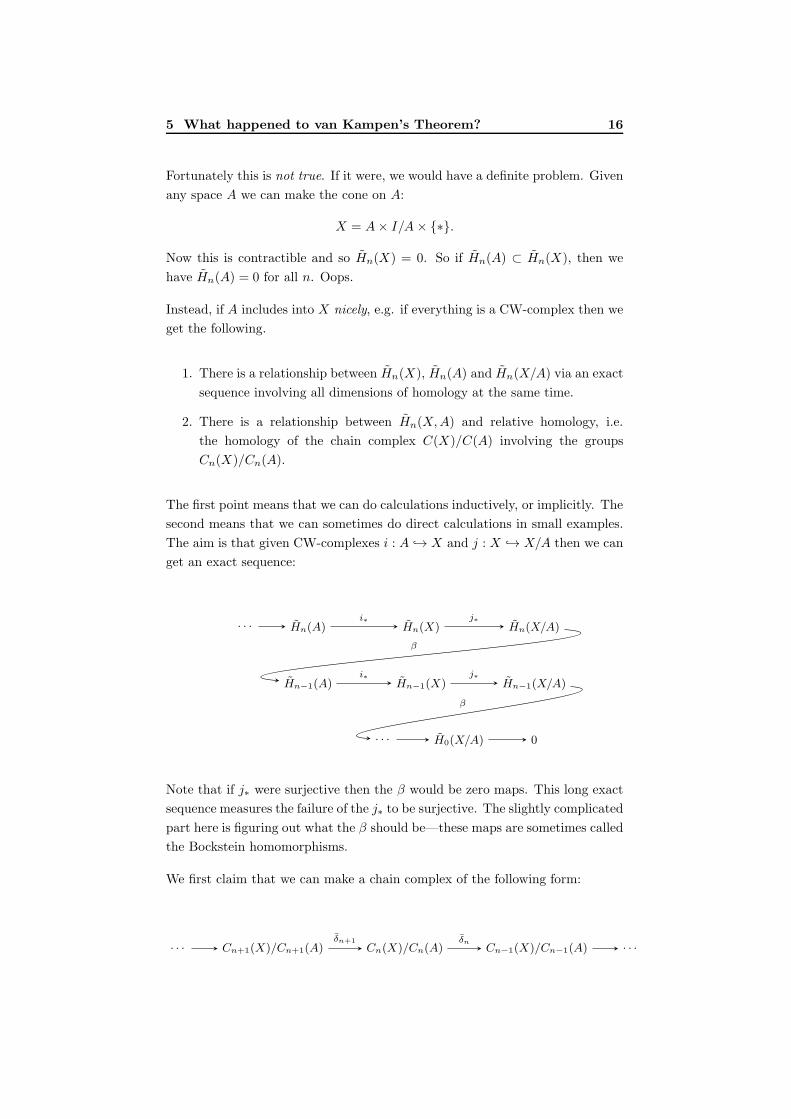
The aim is that given CW-complexes i : A → X and j : X → X/A then we can
get an exact sequence:
· · · Hn(A) Hn(X) Hn(X/A)
Hn−1(A) Hn−1(X) Hn−1(X/A)
· · · H0(X/A) 0
i∗ j∗
β
i∗ j∗
β
Note that if j∗ were surjective then the β would be zero maps. This long exact
sequence measures the failure of the j∗ to be surjective. The slightly complicated
part here is figuring out what the β should be—these maps are sometimes called
the Bockstein homomorphisms.
We first claim that we can make a chain complex of the following form:
· · · Cn+1(X)/Cn+1(A) Cn(X)/Cn(A) Cn−1(X)/Cn−1(A) · · ·δn+1 δn

5 What happened to van Kampen’s Theorem? 17
This works since δn(Cn(A)) ⊂ Cn−1(A). This is called the relative chain com-
plex, the elements of Cn(X)/Cn(A) are called the relative chains and the ho-
mology is called the relative homology, Hn(X,A).
Our second claim is, for all n, Hn(X,A) ∼= Hn(X/A). Note that we don’t have
to reduce relative homology, it happens in the process. (Think about what
happens for the point.)
Example 5.1. Let X = I and A = {0, 1}. Then X/A = S1 and, for all n ≥ 0,
Hn(X,A) ∼= Hn(S1).
Now our third claim is that we have a short exact sequence of Cn’s:
0 Cn(A) Cn(X) Cn(X)/Cn(A) 0
This unravels to a long exact sequence of homology which includes the relative
homology groups and the Bockstein homomorphisms.
· · · Hn(A) Hn(X) Hn(X,A)
Hn−1(A) Hn−1(X) Hn−1(X,A) · · ·
β
Then in nice spaces this gives us the long exact sequence for quotients. In fact
we also have a short exact sequence of chain complexes which we will use after
proving the following lemma.
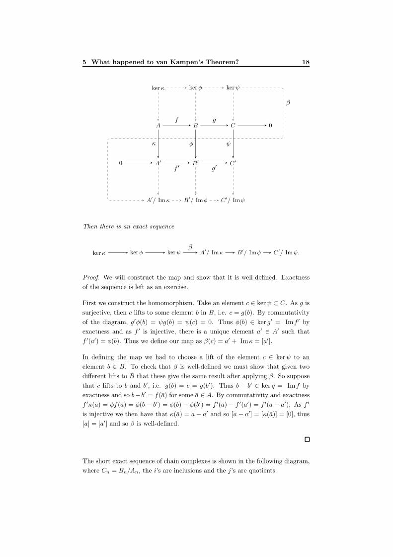
Lemma 5.2 (Snake Lemma). Consider the following diagram of abelian groups
and group homomorphisms, for which the central diagram is commutative and
the middle two rows are exact.
5 What happened to van Kampen’s Theorem? 18
kerκ kerφ kerψ
A B C 0
0 A′ B′ C′
A′/ Imκ B′/ Imφ C′/ Imψ
β
f g
f ′ g′
κ φ ψ
Then there is an exact sequence
kerκ kerφ kerψ A′/ Imκ B′/ Imφ C′/ Imψ.β
Proof. We will construct the map and show that it is well-defined. Exactness
of the sequence is left as an exercise.
First we construct the homomorphism. Take an element c ∈ kerψ ⊂ C. As g is
surjective, then c lifts to some element b in B, i.e. c = g(b). By commutativity
of the diagram, g′φ(b) = ψg(b) = ψ(c) = 0. Thus φ(b) ∈ ker g′ = Imf ′ by
exactness and as f ′ is injective, there is a unique element a′ ∈ A′ such that
f ′(a′) = φ(b). Thus we define our map as β(c) = a′ + Imκ = [a′].
In defining the map we had to choose a lift of the element c ∈ kerψ to an
element b ∈ B. To check that β is well-defined we must show that given two
different lifts to B that these give the same result after applying β. So suppose
that c lifts to b and b′, i.e. g(b) = c = g(b′). Thus b − b′ ∈ ker g = Imf by
exactness and so b− b′ = f(a) for some a ∈ A. By commutativity and exactness
f ′κ(a) = φf(a) = φ(b − b′) = φ(b) − φ(b′) = f ′(a) − f ′(a′) = f ′(a − a′). As f ′
is injective we then have that κ(a) = a− a′ and so [a− a′] = [κ(a)] = [0], thus
[a] = [a′] and so β is well-defined.
The short exact sequence of chain complexes is shown in the following diagram,
where Cn = Bn/An, the i’s are inclusions and the j’s are quotients.
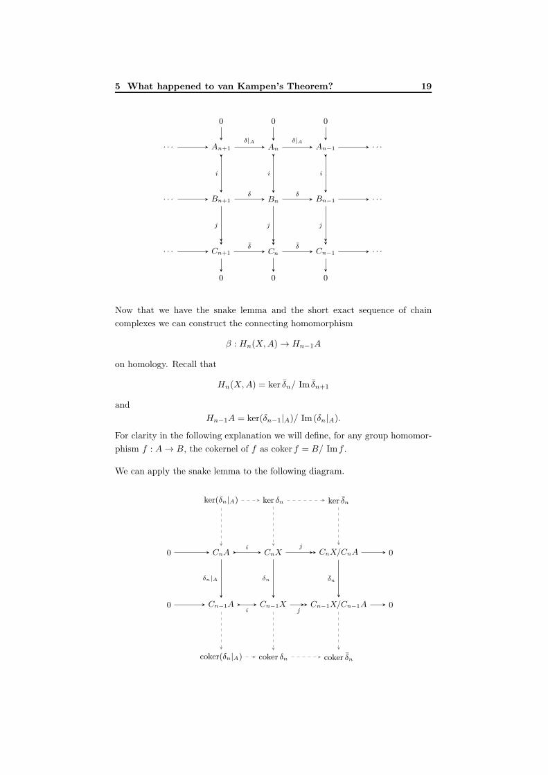
5 What happened to van Kampen’s Theorem? 19
0 0 0
· · · An+1 An An−1 · · ·
· · · Bn+1 Bn Bn−1 · · ·
· · · Cn+1 Cn Cn−1 · · ·
0 0 0
δ|A δ|A
δ δ
δ δ
i i i
j j j
Now that we have the snake lemma and the short exact sequence of chain
complexes we can construct the connecting homomorphism
β : Hn(X,A) → Hn−1A
on homology. Recall that
Hn(X,A) = ker δn/ Im δn+1
and
Hn−1A = ker(δn−1|A)/ Im(δn|A).
For clarity in the following explanation we will define, for any group homomor-
phism f : A→ B, the cokernel of f as coker f = B/ Imf .
We can apply the snake lemma to the following diagram.
ker(δn|A) ker δn ker δn
0 CnA CnX CnX/CnA 0
0 Cn−1A Cn−1X Cn−1X/Cn−1A 0
coker(δn|A) coker δn coker δn
j
j
i
i
δn|A δn δn
6 Quotients and relative homology 20
This gives a homomorphism β : ker δn → coker(δn|A) = Cn−1A/ Im(δn|A).
Now recall the way in which we define the map β. We start with an element
x ∈ ker δn and lift it to x ∈ CnX . This is sent to Cn−1X via δn and is
uniquely lifted to δnx ∈ Cn−1A. Now δn−1|Aδnx = δn−1δnx = 0 and so δnx ∈
ker δn−1|A. Thus β is in fact a map ker δn → ker δn−1|A/ Imδn|A = Hn−1A.
Now as Im δn+1 ⊂ ker δn then we can form a new group homomorphism β :
ker δn/ Im δn+1 = Hn(X,A) → Hn−1A.
6 Quotients and relative homology
In this section we will look more closely at the relationship between relative
homology and the homology of quotient spaces.
Theorem 6.1. Given CW-complexes A ⊂ X, then
1. The quotient maps X → X/A and A → A/A = {∗} induce an isomor-
phism
Hn(X,A)−→Hn(X/A,A/A) = Hn(X/A, ∗)
on homology groups.
2. In general, Hn(Y, ∗) ∼= Hn(Y ) if Y is a CW-complex.
3. There is an isomorphism Hn(X,A)−→Hn(X/A).
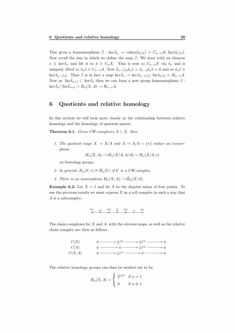
Example 6.2. Let X = I and let A be the disjoint union of four points. To
use the previous results we must express X as a cell complex in such a way that
A is a subcomplex.
x1 x2 x3 x4a b c
The chain complexes for X and A, with the obvious maps, as well as the relative
chain complex are then as follows.
C(X) 0 Z⊕3
Z⊕4 0
C(A) 0 0 Z⊕4 0
C(X,A) 0 Z⊕3 0 0
The relative homology groups can then be worked out to be
Hn(X,A) =
Z⊕3 if n = 1
0 if n 6= 1
6 Quotients and relative homology 21
The quotient space X/A is the wedge sum of three circles S1 ∨ S1 ∨ S1 which
has the following augmented chain complex.
0 Z⊕3 Z Z 0δ1 ǫ
The boundary map δ1 is a zero map, so the reduced homology of X/A is then
the same as the relative homology, for all n.
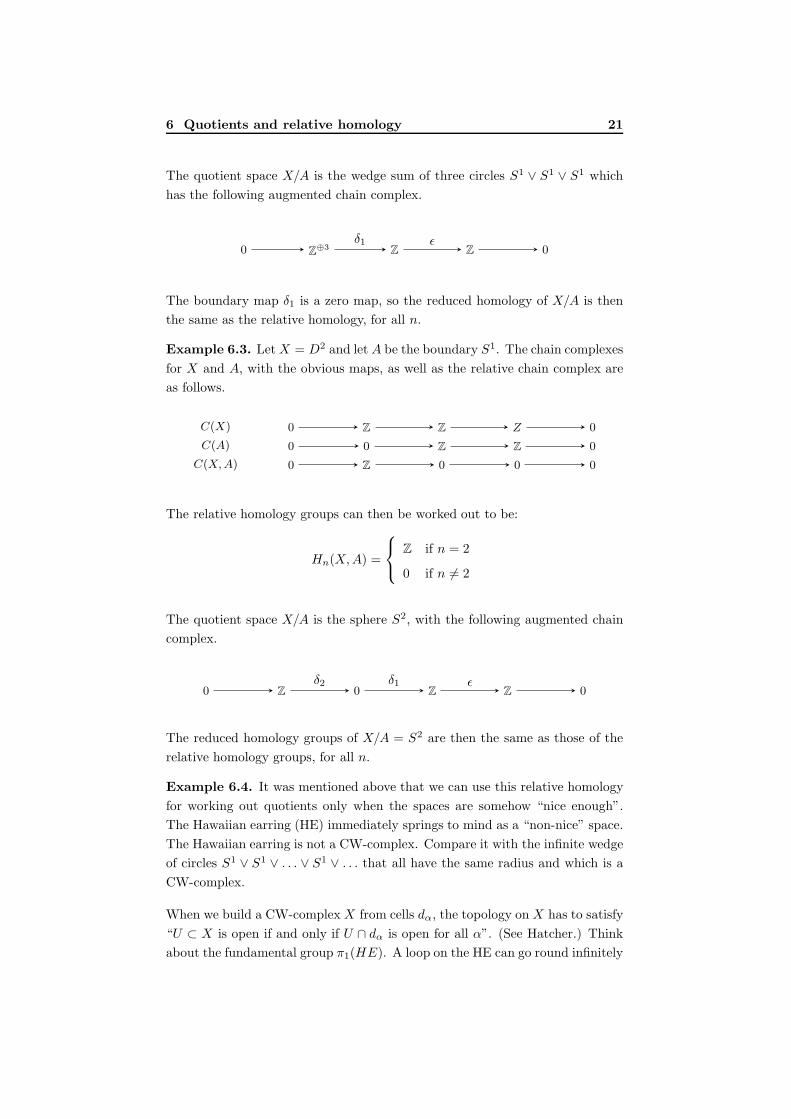
Example 6.3. LetX = D2 and let A be the boundary S1. The chain complexes
for X and A, with the obvious maps, as well as the relative chain complex are
as follows.
C(X) 0 Z Z Z 0
C(A) 0 0 Z Z 0
C(X,A) 0 Z 0 0 0
The relative homology groups can then be worked out to be:
Hn(X,A) =
Z if n = 2
0 if n 6= 2
The quotient space X/A is the sphere S2, with the following augmented chain
complex.
0 Z 0 Z Z 0δ2 δ1 ǫ
The reduced homology groups of X/A = S2 are then the same as those of the
relative homology groups, for all n.
Example 6.4. It was mentioned above that we can use this relative homology
for working out quotients only when the spaces are somehow “nice enough”.
The Hawaiian earring (HE) immediately springs to mind as a “non-nice” space.
The Hawaiian earring is not a CW-complex. Compare it with the infinite wedge
of circles S1 ∨ S1 ∨ . . . ∨ S1 ∨ . . . that all have the same radius and which is a
CW-complex.
When we build a CW-complex X from cells dα, the topology on X has to satisfy
“U ⊂ X is open if and only if U ∩ dα is open for all α”. (See Hatcher.) Think
about the fundamental group π1(HE). A loop on the HE can go round infinitely

6 Quotients and relative homology 22
many different circles. Thus π1(HE) contains ZN as a proper subgroup as we
are then allowed infinitely long words in the generators.
A way to build the Hawaiian earring is to start with the interval, so let X = I,
and take the subspace of points A = { 1n|n ∈ N ∪ {0}}. The quotient space is
then just X/A. (Draw it!) The chain complexes for X and A, as well as the
relative chain complex are as follows.
C(X) 0 ZN
ZN 0
C(A) 0 0 ZN 0
C(X,A) 0 ZN 0 0
Thus the relative homology groups are given by
Hn(X,A) =
ZN if n = 1
0 if n 6= 1
However we know that ZN is a proper subgroup of π1(HE) = H1(HE)ab and
so H1(X,A) ≇ H1(X/A).
As relative homology corresponds, in the right cases, to reduced homology of
quotients then it makes sense to have the rest of the long exact sequence to
also be reduced. We do the same process as we did above with the short ex-
act sequence of chain complexes but we now use the short exact sequence of
augmented chain complexes.
Example 6.5 (Homology of spheres). The circle, or 1-sphere, S1 has trivial
homology except for H1 which is Z. Likewise the 2-sphere S2 has trivial homol-
ogy except for H2 which is Z. Intuitively we’d then think that Sk has trivial
homology except for having Hk(Sk) = Z.
Let X = Dk and A = Sk−1, so that X/A = Sk. The long exact sequence of
reduced homology for these spaces is then as follows.
· · · Hn(Sk−1) Hn(D
k) Hn(Dk, Sk−1)
Hn−1(Sk−1) Hn−1(D
k) · · ·
· · · H0(Dk, Sk−1) 0
β
6.1 Mayer-Vietoris Sequence 23
We know that Dk is contractible and so Hn(Dk) = 0 for all n. Placing these
zeros into the long exact sequence we see that we have many instances of short
exact sequences which in turn means that the Bockstein homomorphisms, β, are
all isomorphism. I.e. Hn(Sk) ∼= Hn(D
k, Sk−1) ∼= Hn−1(Sk − 1) for all n > 0.
Also note that S0 is a pair of points but otherwise Sk is path connected for
k > 0. Thus the 0th homology group of the spheres is given by
H0(Sk)
Z if k = 0
0 if k 6= 0
The remaining piece to find is the homology groups of S0 which are plainly
given by
Hn(S0) =
Z if n = 0,
0 if n 6= 0.
Proceeding by induction we can then prove that
Hn(Sk) =
Z if n = k,
0 if n 6= k.
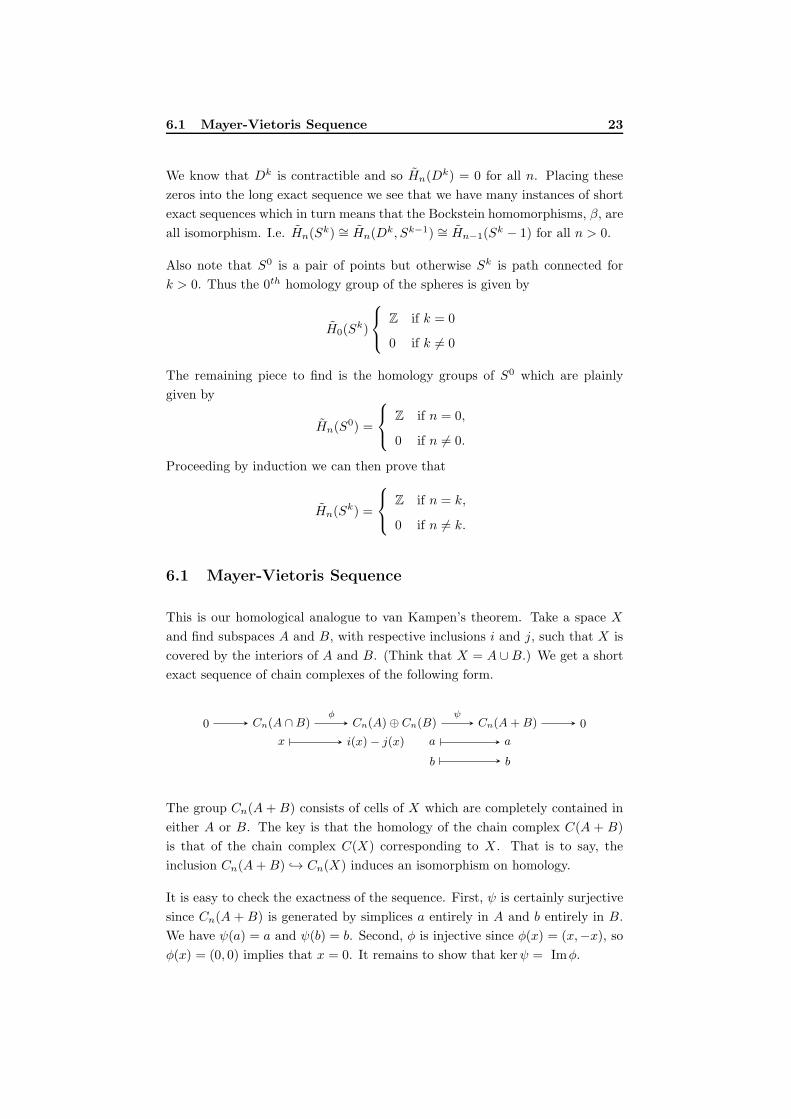
6.1 Mayer-Vietoris Sequence
This is our homological analogue to van Kampen’s theorem. Take a space X
and find subspaces A and B, with respective inclusions i and j, such that X is
covered by the interiors of A and B. (Think that X = A ∪B.) We get a short
exact sequence of chain complexes of the following form.
0 Cn(A ∩B) Cn(A)⊕ Cn(B) Cn(A+B) 0
x i(x)− j(x) a a
b b
φ ψ
The group Cn(A+ B) consists of cells of X which are completely contained in
either A or B. The key is that the homology of the chain complex C(A + B)
is that of the chain complex C(X) corresponding to X . That is to say, the
inclusion Cn(A+B) → Cn(X) induces an isomorphism on homology.
It is easy to check the exactness of the sequence. First, ψ is certainly surjective
since Cn(A + B) is generated by simplices a entirely in A and b entirely in B.
We have ψ(a) = a and ψ(b) = b. Second, φ is injective since φ(x) = (x,−x), so
φ(x) = (0, 0) implies that x = 0. It remains to show that kerψ = Imφ.

7 Axioms for homology 24
First, ψ(φ(x)) = (ψ(x,−x)) = x − x = 0, so Imφ ⊂ kerψ. Now consider
(a, b) ∈ kerψ, i.e. a+b = 0 in Cn(A+B). Then a = −b, so (a, b) = φ(a) ∈ Imφ.
Thus the sequence is exact.
Using the same techniques as before, this unravels to a long exact sequence of
homology.
· · · Hn(A ∩B) Hn(A)⊕Hn(B) Hn(X)
Hn−1(A ∩B) Hn−1(A)⊕Hn−1(B) · · ·
· · · H0(A)⊕H0(B) H0(X) 0
β
Exercise 6.6. Let X = Sn and take A and B to be the north and south hemi-
spheres, Dn, of X . Use the Mayer-Vietoris sequence to work out the homology
of X .
7 Axioms for homology
We will now look at the general idea of homology and what we expect it to do.
Formally, homology is a functor, for all n, from the category of pairs of spaces
(with appropriate maps) to Ab taking a pair (X,A) of spaces to a homology
group Hn(X,A). This should be homotopy invariant together with, for all n, a
map
δn : Hn(X,A) → Hn−1(A,∅)
such that for all maps f : (X,A) → (Y,B), the following square commutes.
Hn(X,A) Hn(Y,B)
Hn−1(A,∅) Hn−1(B,∅)
Hnf
(δn)(X,A) (δn)(Y,B)
Hn−1f
This in fact constitutes what is called a natural transformation. All of the above
is also required to satisfy the following axioms.

8 Further remarks 25
Axiom 7.1 (Dimension). If X is a point, then H0(X) = Z and is the trivial
group otherwise. (In fact we could create a homology theory using any G, not
just Z.)
Axiom 7.2 (Exactness). The following sequence is exact:
· · · Hn(A) Hn(X) Hn(X,A) Hn−1(A) · · ·δ
Axiom 7.3 (Excision). If X is covered by the interiors of A and B then the in-
clusion (B,A∩B) → (X,A) induces an isomorphismHn(B,A∩B)−→Hn(X,A).
Axiom 7.4 (Additivity). If (X,A) = ∐i(Xi, Ai) then there are inclusions
(Xi, Ai) → (X,A) inducing an isomorphism
⊕iHn(Xi, Ai)−→Hn(X,A).
NB. There would be a fifth axiom (Homotopy) if we weren’t restricting to nice
spaces. The five axioms are collectively known as the Eilenberg-Steenrod axioms
for homology theories.
Theorem 7.5. Homology theories are unique.
8 Further remarks
8.1 Moore spaces
Given an abelian group G and an integer n ≥ 1 we can make a CW-complex X
such that
Hi(X) =
G if i = n,
0 if i 6= n.
This is called the Moore space M(G,n). The version for homotopy groups is
denoted K(G,n), the Eilenberg-Mac Lane spaces.
8.2 Wedge sums
Consider a family of based spaces (CW-complexes) (Xα, xα) and consider the
wedge sum of these spaces, ∨α(Xα, xα).
Theorem 8.1. Let (Xα, xα) be a family of based topological spaces, as above.
Then for all n,
Hn(∨α(Xα, xα)) ∼= ⊕αHn((Xα, xα)).
8.3 Suspension 26
Proof. Put X = ∐αXα and A = ∐α{xα}. Then X/A = ∨α(Xα, xα). We know
that Hn(X/A) = Hn(X,A), so
Hn(X,A) = ⊕αHn(Xα, {xα}) ∼= ⊕αHn(Xα),
as required.
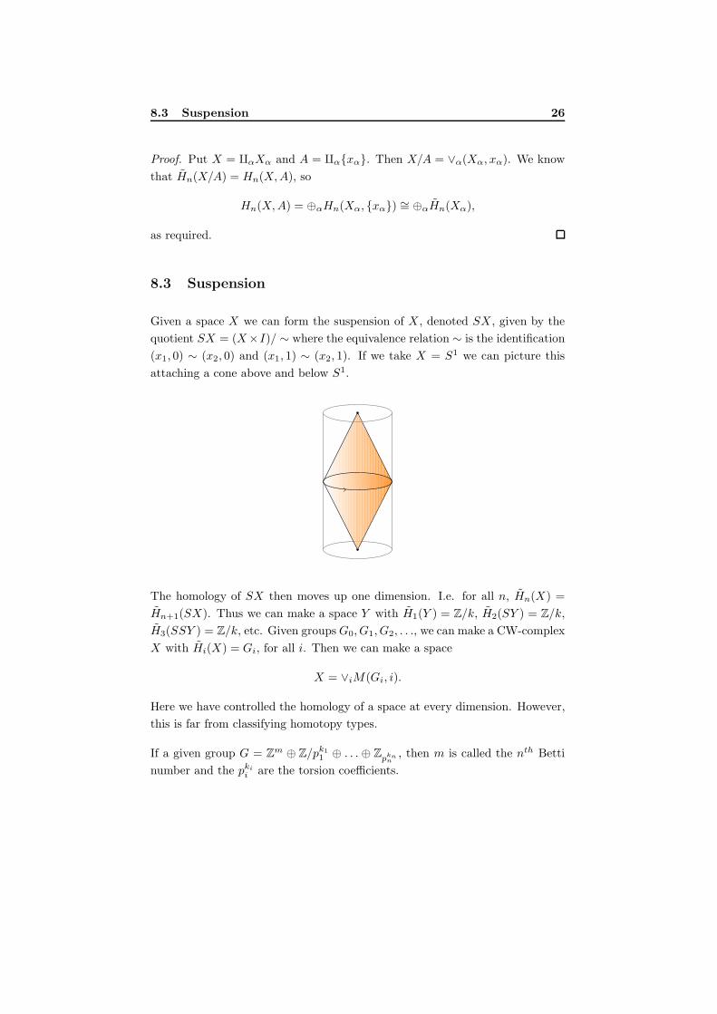
8.3 Suspension
Given a space X we can form the suspension of X , denoted SX , given by the
quotient SX = (X×I)/ ∼ where the equivalence relation ∼ is the identification
(x1, 0) ∼ (x2, 0) and (x1, 1) ∼ (x2, 1). If we take X = S1 we can picture this
attaching a cone above and below S1.
The homology of SX then moves up one dimension. I.e. for all n, Hn(X) =
Hn+1(SX). Thus we can make a space Y with H1(Y ) = Z/k, H2(SY ) = Z/k,
H3(SSY ) = Z/k, etc. Given groupsG0, G1, G2, . . ., we can make a CW-complex
X with Hi(X) = Gi, for all i. Then we can make a space
X = ∨iM(Gi, i).
Here we have controlled the homology of a space at every dimension. However,
this is far from classifying homotopy types.
If a given group G = Zm ⊕ Z/pk11 ⊕ . . . ⊕ Zpknn, then m is called the nth Betti
number and the pkii are the torsion coefficients.