maryland climate action plan
TRANSCRIPT

Appendix D
Maryland Climate Action Plan
Greenhouse Gas & Carbon Mitigation Working Group
Policy Option Documents
Contents
D-1 Agriculture, Forestry & Waste D-2 Energy Supply D-3 Residential, Commercial & Industrial D-4 Transportation & Land Use D-5 Cross-Cutting Issues
Maryland Climate Action Plan
Appendix D-1
Agriculture, Forestry & Waste Management

Maryland Climate Action Plan Appendix D-1
Appendix D-1 Page 2
Agriculture, Forestry, and Waste Management
Introduction The benefits of forests and trees are extensive, complex, and beyond measure. Trees remove carbon dioxide (CO2) from the air and store carbon (C) in their trunks and branches; trees absorb and filter nitrogen dioxide (NO2), sulfur dioxide (SO2), ozone (O3), carbon monoxide (CO), and particulate matter; trees release oxygen and intercept rainwater and dust. The process of evapotranspiration and shade from trees lowers summertime air and surface temperatures.
Shade and lower surface temperatures reduce the need for air conditioning in buildings, thereby reducing the need for the production and transmission of electricity. Reduced energy production reduces emissions of greenhouse gases (GHGs) and carbon from power plants. Shade and lower surface temperatures reduce maintenance needs of infrastructure which, in turn, reduces the conversion of raw materials to asphalt and concrete, which reduces the production of GHGs from manufacturing plants, transportation, and heavy equipment. Shade and lower surface temperatures reduce the evaporation of chemicals from car engines, and reduce the need for air conditioning in cars. This reduces the amount of fuel burned and emissions from cars. And these are but a few examples.
Sustainable forest and urban forest management is essential to healthy, productive forests and trees that maximize mitigation for GHGs and carbon sequestration. Additionally, these forests serve as the preferred land use for avoiding emissions. In the face of climate change, it is critical that everything possible is done to increase the amount of, and enhance the condition of forests and trees everywhere. Healthy forests and trees are our single most cost-effective tool for mitigating for climate change.

Maryland Climate Action Plan Appendix D-1
Appendix D-1 Page 3
Summary List of Recommended Priority Policy Options for Analysis
GHG Reductions (MMtCO2e)
Option No. Policy Option
2012 2020 Total 2008–2020
Net Present Value 2008–2020
(Million $)
Cost- Effective-
ness ($/tCO2e)
Level of Support
AFW-1 Forest Management for Enhanced Carbon Sequestration* 0.04 0.09 0.66 $89.10 $135 Unanimous
AFW-2 Managing Urban Trees and Forests for Greenhouse Gas (GHG) Benefits* 0.73 1.90 13.27 –
$2,017.00 –$152 Unanimous
Afforestation, Reforestation, and Restoration of Forests and Wetlands
Afforestation 0.21 0.6 3.9 $112.70 $29 AFW-3
Riparian areas 0.01 0.05 0.25 $11.00 $44
Unanimous
Protection and Conservation of Agricultural Land, Coastal Wetlands, and Forested Land
Agricultural land 0.11 0.28 1.93 $168.60 $87 Coastal Wetlands N/Q N/Q N/Q N/Q N/Q
AFW-4
Forested land 2.2 2.7 30.5 $1,128.7 $37
Unanimous
“Buy Local” Programs for Sustainable Agriculture, Wood, and Wood Products
Farmers’ Market 0.01 0.03 0.20 –$33.10 –$167 Local Produce N/Q N/Q N/Q N/Q N/Q
AFW-5
Locally Grown and Processed Lumber N/Q N/Q N/Q N/Q N/Q
Unanimous
Expanded Use of Forest and Farm Feedstocks and By-Products for Energy Production
Biomass (Including Agricultural Residue, Forest Feedstocks, and Energy Crops) 0.12 0.50 2.83 $34.10 $12
AFW-6
Methane (CH4) Utilization From Livestock Manure and Poultry Litter 0.01 0.04 0.25 $0.06 $0.2
Unanimous
In-State Liquid Biofuels Production Ethanol Study presented for informational purposes only AFW-7 Bio-diesel 0.10 0.17 1.41 $10.50 $7
Unanimous
AFW-8 Nutrient Trading With Carbon Benefits 0.05 0.14 0.99 –$29.70 –$30 Unanimous
AFW-9 Waste Management Through Source Reduction (SR) and Advanced Recycling 8.80 29.27 184.00 –$1,118 –$6 Unanimous
Sector Totals 12.39 35.77 240.19 -$1643.04 –$7 Sector Total After Adjusting for Overlaps† 5.62 7.53 83.48 –$159.96 -$2 Reductions From Recent Actions – – – – – Sector Total Plus Recent Actions – – – – –
GHG = greenhouse gas; MMtCO2e = million metric tons of carbon dioxide equivalent; $/tCO2e = dollars per metric ton of carbon dioxide equivalent; N/Q = not quantified; CH4 = methane; SR = source reduction.
Note that negative costs represent a monetary savings.
* With Mitigation of Forest Loss Due to Insects, Disease, Pests, and Invasive Species † See next page for discussion of overlap adjustments.

Maryland Climate Action Plan Appendix D-1
Appendix D-1 Page 4
Overlap Discussion The amount of CO2 emissions reduced or sequestered in the policy options within the Agriculture, Forestry, and Waste Management (AFW) sector overlaps with some of the quantified benefits and costs of policy options within other sectors. Those overlaps were identified and adjusted to eliminate double counting. The AFW sector totals were reduced accordingly, as displayed in the Summary List above. The following overview identifies specifically where those overlaps occurred and how they were resolved.
AFW-2 addresses planting trees in urban settings. The Residential, Commercial, and Industrial (RCI) Sector also indirectly includes some tree planting to reduce energy use in buildings as part of demand-side management (DSM) and other energy efficiency programs. AFW-2 addresses urban tree canopies, existing buildings, and carbon sequestration. Only a portion of the CO2 reductions in AFW-2 is based on energy savings from shading and protection of buildings by trees. RCI options broadly address specifically planting trees to affect energy savings in buildings across the entire state. Therefore, only 30% of the emission reductions attributable to energy savings were removed from the AFW quantifications as overlap. The related costs were then adjusted accordingly.
AFW-6 outlines how biomass may be utilized for energy production. The Energy Supply (ES) sector also quantified the use of biomass for energy production. All emission reductions and costs associated with biomass-to-energy production have been removed from AFW sector in the Sector Total After Adjusting for Overlaps row and are accounted for in ES.
AFW-7 focuses on biofuels. The availability of biomass in, and in proximity to Maryland was determined and added a constraint on the amount of energy and biofuels that could be produced. Since ethanol production is addressed in the Transportation and Land Use (TLU) sector, and since that analysis accounts for the use of available biomass for ethanol, all quantifications for AFW ethanol options have been eliminated from the total. Bio-diesel production benefits and savings in AFW were reduced to the production expected from the remaining available biomass after the TLU bio-diesel targets were met.
AFW-9 addresses reduction of waste and recycling. The raw numbers reflect the savings in all GHG emissions and costs from raw material extraction through production as well as waste stream. In the Inventory and Forecast (I&F), only the emissions produced from landfills, waste combustion, wastewater treatment and residential burning were included. Therefore, the portion of emissions and costs over and above the emissions for landfills and waste combustion were eliminated so as to more accurately reflect the difference between Business-As-Usual (BAU) trends as predicted in the Inventory and Forest and the implementation of this policy option. However, addressing waste effectively creates significant emission reductions and cost savings beyond what is now reflected in the adjusted total.

Maryland Climate Action Plan Appendix D-1
Appendix D-1 Page 5
AFW-1. Forest Management for Enhanced Carbon Sequestration
Policy Description Healthy, sustainable, and productive forests provide a vast array of benefits. Sustainable forest management enhances environmental benefits and increases social and economical benefits as well. This policy enhances productivity of healthy, sustainable forests. Benefits from this option include increased rates of CO2 sequestration in forest biomass through healthier forests, increased amounts of carbon stored in harvested, durable wood products, and the availability of renewable biomass for energy production.
Healthy and vigorous forests provide direct benefits to GHG reductions, as noted above, but also serve as the preferred land-use for avoiding emissions and capturing airborne GHGs. To protect those forests so they are able to meet the desired GHG objectives, it is incumbent upon the owner of those forests to attend to the necessary stewardship activities needed to keep the forests healthy and vigorous.
Practices may include supplemental planting on poorly stocked lands, age extension of managed stands, thinning and density management, fertilization and wood waste recycling, expanded use of short-rotation woody crops (for fiber and energy), expanded use of genetically preferred species, modified biomass removal practices, or fire management and risk reduction.
Programs that reduce populations of invasive and damaging insects, diseases, plants, and other pests enhance forest health and long-term sustainability. Reducing pressure from invasive species increases benefits from forests, helps mitigate GHG emissions, and sequesters more carbon. Threats from invasive species are increasing in number and severity, especially since forestlands are more vulnerable due to cumulative effects of other stressors. Some native species populations exceed the carrying capacity of the habitat, undermining regeneration efforts, and therefore sustainability. For example, the overabundance of white-tailed deer places excessive browse pressure on regeneration and understory plants in all forests. It is difficult to quantify the effects of invasive species growth on emissions because the costs of implementation and the efficacy of management strategies can vary widely.
Sustainable forest management is the practice of managing forest resources to meet the long-term forest product needs of humans while maintaining the biodiversity of forested landscapes. The primary goal is to restore, enhance, and sustain a full range of forest values—economic, social, and ecological.
Policy Design Education and outreach, especially for citizens and land managers, will be an important part of this goal to underscore the importance of forests and to teach best management practices (BMPs) for forests.
Goals Related to Forest Management: • Improve sustainable forest management on 25,000 acres of private land by 2020.

Maryland Climate Action Plan Appendix D-1
Appendix D-1 Page 6
• Improve sustainable forest management on 100% of state-owned resource lands by 2020.
Goals Related to Forest Pests and Invasive Species (not quantified): • Develop a prioritization process for invasive species, identifying species of high priority for
targeted action. • Shift decision-making efforts to plan ahead for invasive species problems—move towards
prevention or proactive management rather than control and reactive treatments.
Parties Involved: Maryland Department of Natural Resources (DNR), Maryland Department of the Environment (MDE), Maryland Department of Agriculture (MDA), Maryland Department of Transportation (MDOT), Maryland State Highway Administration (SHA), counties, Chesapeake Bay Program, Natural Resource Conservation Service (NRCS), United States Forest Service–State and Private Forestry (USFS-SPF), United States Fish and Wildlife Service (USFWS), private landowners, public landowners, private sawmills, landscaping industry, nursery industry, Maryland Cooperative Extension (MCE), master gardeners, and the artisan community.
Implementation Mechanisms • Provide outreach and education on best forest management practices.
• Provide outreach and education about invasive species and control methods. • Revise the Forest Conservation Management Act (FCMA) to be consistent with the
recommendations contained herein. • Use a bona fide certification system1 with the aim of certifying all state-owned forestlands as
sustainably managed. • Support a Sustainable Forestry Act that encourages enhanced carbon storage in forests, use of
durable wood products, and use of wood biomass for energy, while maintaining healthy forest ecosystems.
• Use offset funds to enhance forest management on private lands and reduce conversion to other land uses. See Related Polices/Programs in Place.
• Include sustainable forest management in the Regional Greenhouse Gas Initiative (RGGI) Model Rule.
• Develop a mechanism to aggregate products from smaller land holdings to compete in meaningful markets.
• Investigate the feasibility of legislation restricting the sale of priority non-native invasive species.
1 Forest certification is a system for identifying well-managed forestland. In this context, sustainability includes maintenance of ecological, economic, and social components. Products from certified forestland can, through chain-of-custody certification, move into production streams and in the end receive labeling that allows customers to know the product came from a certified, well-managed forest. Fully implemented, certification will become a market-based mechanism to reward superior forest management. The Forest Stewardship Council (FSC) is a nongovernmental, international organization that accredits third-party certifiers and facilitates development of forest management standards. Certifiers include Scientific Certification Systems (California), SmartWood (New York), and regional affiliates.

Maryland Climate Action Plan Appendix D-1
Appendix D-1 Page 7
Related Policies/Programs in Place • FCMA
• Incentive programs for private forestland owners (e.g., Woodland Incentive Program, Forest Conservation and Management Agreements, Woodland Assessment Program, and the Tax Modification for Forest Management program), which provide either cost-share funds or tax breaks for appropriate management of their forests.
• U.S. Department of Agriculture (USDA) programs for forests and related wetlands and USFWS reforestation and wetlands programs for habitat improvement.
Type(s) of GHG Reductions CO2 (quantified): Enhancement of annual carbon sequestration from forest growth and reforestation through forestry management programs.
CO2 (not quantified): Remove fuels that contribute to wildfire emissions. Maintain carbon sequestration through the production of durable wood products. Reduce emissions by reducing use of fossil fuels and replace them with energy from woody biomass. Reduce emissions by preventing the release of carbon from dead and dying trees. Reduce wildfire emissions by maintaining healthy forests.
Estimated GHG Reductions and Net Costs or Cost Savings Data Sources: • Forest-type distribution in Maryland and landownership statistics from the USDA Forest
Inventory and Analysis (FIA), available at: http://fia.fs.fed.us. • J.E. Smith, L.S. Heath, K.E. Skog, and R.A. Birdsey. 2006. Methods for calculating forest
ecosystem and harvested carbon with standards estimates for forest types of the United States. USDA United States Forest Service (USFS) Northern Research Station. General Technical Report GTR-NE-343. (Also published as part of the United States Department of Energy [US DOE] Voluntary GHG Reporting Program.) Available at http://www.treesearch.fs.fed.us/pubs/22954 (ne_gtr343.pdf)
Quantification Methods: While experts largely agree sustainably managed forests may store substantially more carbon on an annual basis than forests not managed sustainably, few data are currently available to quantify exactly what kinds of sites can store exactly how much additional carbon, and under what silvicultural regimes. Furthermore, some existing forests are indeed being managed sustainably, such that determining the amount of acreage available for improved forest management can be difficult.
To calculate the effect of improved forest management on carbon sequestration in Maryland, the additional carbon stored as a result was indexed using data on rates of carbon storage in average loblolly-shortleaf pine stands compared with carbon storage rates in high-productivity, intensively managed loblolly-shortleaf pine stands in the Southeast (GTR-NE-343, Tables A39 and A40). The index of incremental carbon storage was calculated over a 90-year period to capture slowdown in forest carbon sequestration that typically occurs in maturing forest stands.

Maryland Climate Action Plan Appendix D-1
Appendix D-1 Page 8
Soil carbon was assumed to remain constant with time, because there is no change in estimates of soil carbon pools over time in the General Guidelines for the Voluntary Reporting of Greenhouse Gases Program (under Section 1605(b) of the Energy Policy Act of 1992). The incremental rate of carbon storage, due to intensive management in loblolly-shortleaf pine stands relative to average loblolly-shortleaf pine stands in the Southeast, is roughly 5% (Table I-1).
Table I-1. Carbon sequestration rates under average and intensive management scenarios for loblolly-shortleaf pine forests in the Southeast United States following clear-cut harvest
Forest Type tC/acre (0 year)
tC/acre (90 year) tC/acre/year
Increment in tC/acre/year
Due to Management Loblolly-shortleaf pine stands (GTR-NE-343, Table A39) 10.7 60.5 0.553
Loblolly-shortleaf pine on high productivity sites under intensive management (GTR-NE-343, Table A40) 14.9 67.0 0.579 5%
tC/acre = metric tons of carbon per acre. Forests in Maryland are 63% oak-hickory, with 10% oak-pine and 11% loblolly-shortleaf pine.2 The remaining 16% of forestland area is a mixture of forest types. Coefficients for improved productivity in oak-hickory and oak-pine stands were not available. The rate of carbon sequestration, due to improved forest management in these forest types, was thus calculated as a proportion of average carbon sequestration in forests under typical management, using the 5% value calculated for incremental carbon storage in loblolly-shortleaf pine stands (Table I-2).
Table I-2. Estimated carbon sequestration rates on forestland under intensive management
Forest Type tC/acre (0 year)
tC/acre (65 year) tC/acre/year
tC/acre/year Under Intensive
Management Oak-hickory (GTR NE 343, Table A3) 23.0 72.7 0.765 0.800
Oak-pine (GTR NE 343, Table A4) 25.9 63.4 0.577 0.604
Loblolly-shortleaf pine (GTR NE343, Table A39) 10.7 51.8 0.632 0.662
tC/acre = metric tons of carbon per acre. Forest carbon sequestration rates under baseline conditions (no improved forest management) were based on published carbon stocks (tons of carbon per acre [tC/acre] in forest biomass) for oak-hickory and oak-pine in the Northeast and for loblolly-shortleaf pine stands in the Southeast (USFS GTR-NE-343). Annual rates of carbon sequestration (tC/acre/year) were calculated by subtracting total carbon stocks in forest biomass of 65-year-old stands from total carbon stocks in 2 USDA USFS Northern Global Change Program, Available at http://www.fs.fed.us/ne/global/pubs/books/epa/states/MD.htm

Maryland Climate Action Plan Appendix D-1
Appendix D-1 Page 9
forest biomass of new stands and dividing by 65. An average for 65-year-old stands was used to reflect the typical stand age of forests in the Northeast region.
Quantification for this option was based on a combined goal of achieving enhanced forest management on 25,000 acres of private land and 100% of state-owned forestland by 2020. Based on 2004 FIA data, state-owned forests total 749,975 acres3 in Maryland, roughly 31.2% of the 2.4 million forested acres statewide. Other forestland ownership entities in the state include the USFWS (42,561 acres), county and municipal government (41,148 acres) and privately owned forests (1,567,846 acres). This acreage includes all land classified as forest by FIA and owned by the State of Maryland, regardless of which branch of state government is currently responsible for managing that forest.
A linear ramp-up in implementation is assumed. Thus, each year from 2008 to 2020, the analysis assumes 1,923 acres of private land and 57,690 acres of public land are added to the land base practicing sustainable forest management. Therefore, the effect of policy implementation is the incremental carbon stored on these lands is over and above expectations if enhanced forest management were not implemented. Baseline and policy implementation scenarios assume the distribution of forests affected by the program will reflect the distribution of forests statewide: 70% oak-hickory, 15% oak-pine, and 15% loblolly-shortleaf pine. Acreage enrolled in the program in one year is assumed to continue sequestering additional carbon in subsequent years. Table I-3 summarizes the total carbon storage resulting from enhanced forest management.
3 USDA USFS FIA EVALIDator version 1.0. Available at http://fiatools.fs.fed.us/

Maryland Climate Action Plan Appendix D-1
Appendix D-1 Page 10
Table I-3. Additional acreage and carbon sequestration resulting from expanded land base participating in sustainable forest management
Year
Private Land Added to
Sustainable Forest
Management This Year
Added in Prior Years
Public Land Added
This Year
Public Land Added in
Prior Years
Additional Carbon Storage (MMtCO2e/year)
2008 1,923 0 57,690 0 0.007
2009 1,923 1,923 57,690 57,690 0.014
2010 1,923 3,846 57,690 115,381 0.022 2011 1,923 5,769 57,690 173,071 0.029
2012 1,923 7,692 57,690 230,762 0.036
2013 1,923 9,615 57,690 288,452 0.043
2014 1,923 11,538 57,690 346,142 0.051
2015 1,923 13,462 5,7690 403,833 0.058
2016 1,923 15,385 57,690 461,523 0.065
2017 1,923 17,308 57,690 519,213 0.072
2018 1,923 19,231 57,690 576,904 0.080 2019 1,923 21,154 57,690 634,594 0.087
2020 1,923 23,077 57,690 692,285 0.094
Total 25,000 749,975 0.658
MMtCO2e = million metric tons of carbon dioxide equivalent. The economic cost of implementing enhanced forest management on forest acreage is a one-time cost (over and above the cost to implement standard management techniques) of improved forest management practices and is estimated to be $151.50/acre. This value is an average of values from other states where similar policy options have been quantified: Vermont, where a value of $3/acre was used,4 and Montana, where a value of $300/acre was used.5 Clearly, there is little consensus about what is required to implement an enhanced forest management program and, as a result, the estimates of how much it will cost to implement these policies varies widely. State-specific data would substantially improve the validity of the estimate of economic costs for this option in Maryland. At $151.50/acre, and using a discount rate of 5%, the net present value (NPV) of this option is $89.1 million (Table I-4), with an overall cost-effectiveness of $135.31 per metric ton of carbon dioxide equivalent (tCO2e) stored.
4 http://www.vtclimatechange.us 5 http://www.mtclimatechange.us

Maryland Climate Action Plan Appendix D-1
Appendix D-1 Page 11
Table I-4. Total economic costs for implementing improved forest management on combined private and public acreage in Maryland
Year Carbon Sequestered
(MMtCO2e/year) Total Cost Discounted Cost 2008 0.007 $9,031,439 $9,031,439
2009 0.014 $9,031,439 $8,601,371
2010 0.022 $9,031,439 $8,191,782
2011 0.029 $9,031,439 $7,801,697
2012 0.036 $9,031,439 $7,430,188
2013 0.043 $9,031,439 $7,076,369
2014 0.051 $9,031,439 $6,739,399 2015 0.058 $9,031,439 $6,418,475
2016 0.065 $9,031,439 $6,112,834
2017 0.072 $9,031,439 $5,821,746
2018 0.080 $9,031,439 $5,544,520
2019 0.087 $9,031,439 $5,280,496
2020 0.094 $9,031,439 $5,029,043
Total 0.658 $117,408,713 $89,079,360
MMtCO2e = million metric tons of carbon dioxide equivalent.
Key Assumptions: • Carbon storage resulting from sustainable management of oak-hickory and oak-pine types is
indexed to incremental carbon storage in loblolly-shortleaf-pine forests, as quantified using methods in GTR-NE-343.
• One-time costs to implement enhanced forest management are $151.50/acre, and include costs over and above standard costs for forest management operations.
• Forest types added to the pool of sustainably managed forests will reflect the distribution of forests statewide.
Key Uncertainties GHG emissions from management activities, such as harvest, are not included in this analysis. To provide clarity about the effects of policy implementation, it is important to quantify the changes in emissions resulting from changes in management practices due to policy implementation.
Additional Benefits and Costs As markets are developed, additional biomass generated via enhanced forest management will be used first for long-term storage in durable wood products and then for beneficial uses, such as biofuels and energy. The biomass generated from improved management practices could be used for durable wood products and energy production. The quantification described above assumes additional carbon is stored in the forest.

Maryland Climate Action Plan Appendix D-1
Appendix D-1 Page 12
Forest certification will likely be necessary for participation in the RGGI market, but effects of certification are not quantified here because effects on carbon storage are uncertain and because the costs are difficult to quantify.
Feasibility Issues Sustainable forest management is well researched, and offers a plethora of mandated and voluntary BMPs. The primary hurdle remains one of education and incentives that will move existing marginal practices or inaction to engaged, sustainable management.
Status of Group Approval Approved.
Level of Group Support Unanimous.
Barriers to Consensus None.

Maryland Climate Action Plan Appendix D-1
Appendix D-1 Page 13
AFW-2. Managing Urban Trees and Forests for Greenhouse Gas (GHG) Benefits
Policy Description Healthy, sustainable urban forests are essential to our social, economic, and environmental welfare. This policy option maintains and improves the health and longevity of trees in urban and residential areas. Trees in urban areas help avoid emissions from power production, and from the operation and maintenance (O&M) of built structures and infrastructure. Further, urban trees contribute to lower summertime temperatures at street level. Reduced heat slows the formation of ground-level O3, as well as the evaporation and volatilization of organic compounds from vehicles. Trees also take in CO2 for photosynthesis, storing carbon in their biomass through growth. Trees likewise reduce ambient concentrations of volatile organic compounds, nitrous oxide (N2O), fine particulate matter, and other air and water pollutants.
Statewide, the urban canopy cover in Maryland is 40.1%.6 This option seeks to increase the canopy cover of urban trees throughout the state. Planting additional trees in-state may: increase the utilization of wood recovered from urban trees for energy production or in value-added products for long-term carbon storage; encourage species diversity while extending survival and longevity rates through the creation of amenable microclimates; and address insects, invasive species, and disease in urban forest settings, though these impacts are not quantified here.
Policy Design Educate the public and legislators on the importance of urban forests for O3 and temperature regulation, leading to reduced energy use.
Goals: • Enhance green infrastructure planning including tying green areas together (not quantified).
• Develop incentives to better use urban wood recovery directed toward the highest-order wood product (not quantified), with the remainder recovered for biomass to energy conversion (see AFW-6).
• Achieve urban tree canopy (UTC) goal of 50% (averaged over all urban land-use types) by 2020.
Goals Related to Forest Pests and Invasive Species (Not Quantified): • Develop prioritization process for invasive species, identifying species of high priority for
targeted action. • Shift decision-making efforts to plan ahead for invasive species problems—move towards
prevention or proactive management, rather than control and reactive treatments.
Timing: See quantified goal above.
6 USDA USFS data (D. Nowak). Available at http://www.fs.fed.us/ne/syracuse/Data/State/data_MD.htm.

Maryland Climate Action Plan Appendix D-1
Appendix D-1 Page 14
Parties Involved: DNR, MDE, MDA, MDOT, SHA, counties, municipalities, Chesapeake Bay Program, NRCS, USFS Urban and Community Forestry, private landowners, public landowners, private sawmills, artisan community, landscaping industry, nursery industry, arborist industry, MCE, and master gardeners.
Implementation Mechanisms • Encourage the funding and expansion of planting programs in all communities, including a
replacement program for dead trees, where a tree with equal potential is planted in a site as good as or better than the original to maximize longevity and efficacy.
• Insert urban tree planting strategy and objectives in all comprehensive plans. • Encourage local counties to identify, maintain, and augment street tree populations.
• Provide outreach and education on the significance of trees and their role in our built environment.
• Monitor and report plantings at the local level. • Provide enhanced funding from conservation programs like Program Open Space (POS) to
local jurisdictions to implement policies (e.g., wood recovery and canopy goals) and to plant trees.
• Implement legislation restricting sale of priority non-native invasive species. • Outreach and education about invasive species and control methods.
• To strengthen, fund, and support this act, add UTC goals to the Urban Community Forest Act.
Related Policies/Programs in Place Urban Community Forestry Act.
Tree-mendous Maryland, a program that, for a fee, individuals can request a tree be planted as a memorial.
Chesapeake Bay Program’s Forest Conservation Directive 2020 goals. The Governor of Maryland committed to establishing urban canopy goals by 2020 for 50% of the area developed before storm-water management regulations (i.e., pre-1984), among other goals.
Community Woodlands Alliance, a group of local artisans building furniture from old-growth urban trees.
Type(s) of GHG Reductions CO2 (quantified): Avoidance of emissions of CO2 and associated GHGs through the reduction of heating and cooling needs in urban areas. Carbon sequestration due to tree growth.
CO2 (not quantified): Decrease in surface temperatures reducing volatilization of gases from vehicles. Maintaining carbon sequestration by creating durable wood products. Reduce use of fossil fuels by using wood waste for energy.

Maryland Climate Action Plan Appendix D-1
Appendix D-1 Page 15
The emissions saved as calculated under this policy option overlap with some options recommended in the RCI Technical Work Group (TWG). These AFW policy emissions are related only to trees in urban settings, whereas the energy-savings emission reductions are calculated across the state under RCI. Therefore, the emission reductions that result from energy savings for this policy option have been reduced by 30% (see Sector Total after Adjusting for Overlap on Summary List.)
Estimated GHG Reductions and Net Costs or Cost Savings Data Sources: • Data about existing and potential UTC cover for Maryland from:
○ M.F. Galvin, J.M. Grove, and J. O’Neill-Dunne. 2006a (Jan.). A report on Baltimore City’s present and potential urban tree canopy. Prepared for The Honorable Mayor Martin O’Malley, City of Baltimore. Available at http://www.dnr.state.md.us
○ M.F. Galvin, J.M. Grove, and J. O’Neill-Dunne. 2006b (June). A report on Annapolis’ present and potential urban tree canopy. Prepared for The Honorable Mayor Ellen O. Moyer, City of Annapolis. Available at http://www.dnr.state.md.us
○ M.F. Galvin, J. O’Neill-Dunne, and J.M. Grove. 2008. A report on the City of Frederick’s existing and possible urban tree canopy. Available at http://www.dnr.state.md.us
• Information about current numbers of trees in urban forest and annual carbon storage in urban trees in Maryland: USDA USFS Northern Research Station. Urban forest effects on environmental quality state summary data for Maryland (2003). Available at http://www.fs.fed.us/ne/syracuse/Data/State/data_MD.htm
• Parameters for energy and emission savings of tree planting: E.G. McPherson and J.R. Simpson. 1999. CO2 reduction through urban forestry: guidelines for professional and volunteer tree planters. USDA USFS Pacific Southwest Research Station. General Technical Report PSW-GTR-171.
• Data on costs and benefits of tree planting: E.G. McPherson et al. 2006. Piedmont community tree guide: benefits, costs, and strategic planting. USDA USFS Pacific Southwest Research Station. General Technical Report PSW-GTR-200.
• Additional data on benefits of tree canopy in Maryland: M.F. Galvin. 2007. A report on Hyattsville’s street trees. Prepared for The Honorable William F. Gardiner, Mayor and James Chandler, Community Development Manager. Available at http://www.dnr.state.md.us
Quantification Methods: The following quantifies the cumulative impact on carbon sequestration and avoided fossil fuel emissions of incrementally increasing the existing tree canopy cover in Maryland. Specifically, AFW-2 seeks to achieve a goal of 50% urban canopy cover by 2020. Currently, Maryland’s urban areas are 40.1% forested.7 This goal recommends a 25% increase over the existing canopy cover by 2020. The goal of 50% is based on recent assessments of existing and potential UTC in Maryland. For example, Baltimore currently has a canopy cover of 20%, and a goal of 46.3% is
7 USDA USFS data (D. Nowak). Available at http://www.fs.fed.us/ne/syracuse/Data/State/data_MD.htm.

Maryland Climate Action Plan Appendix D-1
Appendix D-1 Page 16
recommended as feasible within the 2030–2036 time frame (Galvin et al. 2006a). Annapolis’ urban areas are currently 41% forested, and a 50% goal is recommended within the same time frame (Galvin et al. 2006b). Frederick is currently only 12% forested (Galvin et al. 2008), but there appear to be no obvious barriers to increasing its UTC. While the UTC analyses cited above recommend a longer time frame to reach the UTC targets, this analysis seeks to quantify the effects of policy implementation within the 2008–2020 time frame described by the Mitigation Working Group (MWG).
Currently, Maryland contains 89.4 million urban trees; this option quantifies the effect of adding a total of 22 million new trees by 2020. The number of trees planted each year is constant at roughly 1.7 million/year, with the target number of trees planted by 2020.
GHG benefits are twofold: direct carbon sequestration by planted trees, and avoided GHG emissions from strategic tree planting to reduce energy demand due to heating and cooling.
A. Direct Carbon Sequestration in Urban Trees Annual carbon sequestration per urban tree is calculated as 0.006 metric tons of carbon dioxide equivalents per tree per year (tCO2/tree/year), based on statewide average data reported by the USFS. This is the average annual per-tree carbon sequestration value when the total estimated urban forest carbon accumulation in Maryland (544,000 tCO2/year) is divided by the total number of urban trees in Maryland (89.4 million). Since trees planted in one year continue to accumulate carbon in subsequent years, annual carbon sequestration in any given year is calculated as the sum of carbon stored in trees planted in that year, plus the sequestration by trees planted in prior years. Because it simply takes the difference between total live C stocks at two points in time, this stock change approach accounts for normal tree mortality.
B. Avoided Fossil Fuel Emissions Offsets from avoided fossil fuel use for heating and cooling are the sum of three different types of savings: (1) avoided emissions from reduced cooling demand, (2) avoided emissions from reduced demand for heating due to wind reduction (this benefit is only available for evergreen trees), and (3) enhanced fossil fuel emissions needed for heat due to wintertime shading. Calculations for avoided fossil fuel offsets are based on calculations presented by McPherson et al. (1999) (see Table I-5). For this analysis, it was assumed half of the trees would be planted in residential settings or close enough to buildings to result in avoided emissions. Where plantings are assumed to provide this avoided emissions benefit, it was further assumed the trees planted would be evenly split among residential settings with pre-1950, 1950–1980, and post-1980 homes and all planted are medium-sized evergreens. These avoided emission factors assume average tree distribution around buildings (i.e., these fossil fuel reduction factors are average for existing buildings, but do not necessarily assume trees are optimally placed around buildings to maximize energy efficiency). These factors are also dependent on the fuel mix (e.g., coal, hydroelectric, or nuclear) in the region, and thus are likely to change if the electricity mix changes from its 1999 distribution.

Maryland Climate Action Plan Appendix D-1
Appendix D-1 Page 17
Table I-5. Factors used to calculate CO2e savings (MMtCO2e/tree/year) from reduced need for fossil fuel for heating and cooling and from windbreak effect of evergreen trees
Fossil Fuel Offsets: Evergreen Trees (Mid-Atlantic Climate Region) Housing Vintage Shade–Cooling Shade–Heating Wind–Heating Net Effect Pre-1950 0.0168 –0.0315 0.1294 0.1147
1950–1980 0.0275 –0.0403 0.1555 0.1427
Post-1980 0.0232 –0.0324 0.133 0.1238
Average 0.0225 –0.0347 0.1393 0.1271
Average (MMtCO2e) 1.2707
MMtCO2e = million metric tons of carbon dioxide equivalent.
Source: McPherson et al., 1999
C. Overall GHG Benefit of Urban Tree Planting Total GHG benefits are calculated as the sum of direct carbon sequestration plus fossil fuel offset from reduced cooling demand and wind reduction (Table I-6).
Table I-6. Overall GHG benefit (MMtCO2e/year) of implementing AFW-2
Year Trees Planted
This Year Trees Planted in Previous Years
GHG Sequestered
(MMtCO2e/year)
GHG Avoided
(MMtCO2e/year)
Overall GHG Savings
(MMtCO2e/year) 2008 1,698,440 0 0.0379 0.1079 0.1458
2009 1,698,440 1,698,440 0.0758 0.2158 0.2916
2010 1,698,440 3,396,879 0.1136 0.3237 0.4374
2011 1,698,440 5,095,319 0.1515 0.4316 0.5832
2012 1,698,440 6,793,759 0.1894 0.5395 0.7289
2013 1,698,440 8,492,198 0.2273 0.6474 0.8747
2014 1,698,440 10,190,638 0.2652 0.7554 1.0205
2015 1,698,440 11,889,078 0.3030 0.8633 1.1663 2016 1,698,440 13,587,517 0.3409 0.9712 1.3121
2017 1,698,440 15,285,957 0.3788 1.0791 1.4579
2018 1,698,440 16,984,397 0.4167 1.1870 1.6037
2019 1,698,440 18,682,836 0.4546 1.2949 1.7495
2020 1,698,440 20,381,276 0.4924 1.4028 1.8952
Total 22,079,716 3.4471 9.8196 13.2667
GHG = greenhouse gas; MMtCO2e/year = million metric tons of carbon dioxide equivalent per year.
D. Cost Analysis Economic costs of tree planting are calculated as the sum of tree planting and annual maintenance, including the costs of program administration and waste disposal. Economic benefits of tree planting include the cost offset from reduced energy use, as well as the estimated economic benefits of services (e.g., provision of clean air), hydrologic benefits (e.g., storm water control), and aesthetic enhancement.

Maryland Climate Action Plan Appendix D-1
Appendix D-1 Page 18
The cost of tree planting in Maryland was assumed to be $275/tree.8 This is a one-time cost incurred in the year of planting. Annual maintenance costs include pruning, pest management, administration, removal, and infrastructure repair due to damage from trees. Over a 40-year period, these costs were estimated at $22/tree/year, based on McPherson et al. (2006). This value assumes a medium-sized evergreen tree and is an average of trees under public and private management. This value is consistent with annualized maintenance costs per tree published for other states and regions. It was assumed trees planted in the first year of policy implementation would still be living at the end of the policy implementation period; in other words, the effects of tree mortality are not explicitly accounted for in the analysis of the numbers of trees planted to achieve the canopy goals described above.
The economic benefit of planting urban trees includes the value of aesthetic improvement, air and water quality improvements, stormwater management, and energy savings. Annual economic benefit per tree was estimated at –$96.30/tree/year, using information from Galvin et al. (2007) on the economic value of Hyattsville, Maryland’s urban forest. Consistent with convention, the economic benefit per tree planted is a negative number since the economic benefit outweighs the cost of the option. When the economic benefit of an option outweighs its cost, then the resulting net economic cost is negative.
Net economic costs for this option are calculated as the difference between costs of planting and maintenance and economic benefit realized by urban trees. Therefore, negative costs refer to net economic benefits, where estimated benefits exceed overall costs. For this analysis, net economic benefit per tree was estimated at –$74.30/tree/year. Discounted costs were calculated assuming a 5% discount rate (Table I-7). AFW-2 has a net economic benefit of –$152.00/tCO2e mitigated.
8 Mike Galvin, Supervisor, Urban and Community Forestry, Maryland DNR. Personal communication with J. Jenkins, January 2008. Range of costs estimated at $250-300.

Maryland Climate Action Plan Appendix D-1
Appendix D-1 Page 19
Table I-7. Economic benefits and costs of implementing AFW-2
Year
Trees Planted
This Year
Trees Planted in Previous
Years Total Economic
Benefit Net Benefit
(Costs Minus Benefits) Discounted Net Benefits
2008 1,698,440 0 $0 $467,070,909 $467,070,909
2009 1,698,440 1,698,440 $163,559,740 $340,876,842 $324,644,611
2010 1,698,440 3,396,879 $327,119,480 $214,682,774 $194,723,605 2011 1,698,440 5,095,319 $490,679,221 $88,488,707 $76,439,872
2012 1,698,440 6,793,759 $654,238,961 –$37,705,361 –$31,020,294
2013 1,698,440 8,492,198 $817,798,701 –$163,899,428 –$128,419,491
2014 1,698,440 10,190,638 $981,358,441 –$290,093,496 –$216,472,233
2015 1,698,440 11,889,078 $1,144,918,182 –$416,287,563 –$295,847,799
2016 1,698,440 13,587,517 $1,308,477,922 –$542,481,631 –$367,172,921
2017 1,698,440 15,285,957 $1,472,037,662 –$668,675,698 –$431,034,317
2018 1,698,440 16,984,397 $1,635,597,402 –$794,869,766 –$487,981,084 2019 1,698,440 18,682,836 $1,799,157,142 –$921,063,833 –$538,526,947
2020 1,698,440 20,381,276 $1,962,716,883 –$1,047,257,901 –$583,152,386
Total 22,079,716 $12,757,659,738 –$3,771,215,443 –$2,016,748,473 Key Assumptions: Economic costs and benefits of urban tree cover. Feasibility of accelerated implementation of UTC recommendations. Each community has the capacity and technical skill to assess the appropriate species and location for trees planted.
Key Uncertainties Cities and communities would need to conduct canopy surveys to establish a baseline of current canopy cover. The costs of such a survey and continued monitoring are variable and may exceed available resources. The longevity of urban trees may be affected by climate perturbations.
Additional Benefits and Costs In addition to the numerous benefits articulated in the policy description, urban trees contribute to improved property values, add aesthetic value for residents and visitors, provide humidity balancing, and reduce the intensity of stormwater runoff. Sociological studies suggest that more attractive and comfortable neighborhoods have lower crime rates.
Feasibility Issues Ensuring a constant source of quality urban trees for achieving planting goals without incurring excessive transportation costs is of concern.
Finding the necessary funding in a constant flow per annum is another concern.
Status of Group Approval Approved.

Maryland Climate Action Plan Appendix D-1
Appendix D-1 Page 20
Level of Group Support Unanimous.
Barriers to Consensus None.

Maryland Climate Action Plan Appendix D-1
Appendix D-1 Page 21
AFW-3. Afforestation, Reforestation, and Restoration of Forests and Wetlands
Policy Description Increasing forest and tree cover provides additional benefits for mitigation of GHGs in addition to sequestration. This policy option promotes forest cover and associated carbon stocks by regenerating or establishing healthy, functional forests through afforestation (on lands that have not, in recent history, been forested, including agricultural lands) and reforestation (on lands with little or no present forest cover) where current beneficial practices are not displaced. Successful establishment requires commitment for as long as 20 years. Forest patches should be sufficient in size to function as a community of trees and related species.
In addition, this policy promotes the implementation of practices, such as soil preparation, erosion control, and supplemental planting to ensure conditions that support forest growth. Identify areas, including all wetlands, in need of physical intervention to return forest habitats to full vigor. Additional areas of concern are linking islands of fragmented forests to restore function, recovering severely disturbed lands, and reversing the effects of continued toxicity on those disturbed lands.
Policy Design Carbon sequestration via afforestation is important, but other ancillary benefits provided by forests, in terms of green space, quality of life, and avoided emissions are also critical and add to the value of forestland for the community (see Introduction).
Maryland is a member of the RGGI (http://www.rggi.org), which mandates the existence of an interstate CO2 Budget Trading Program to reduce emissions from the power sector (RGGI applies to fossil fuel-burning plants larger than 25 megawatts [MW]). Beginning with implementation of the CO2 Budget Trading Program on January 1, 2009, emissions entities are permitted to use offset projects to meet up to 3.3% of their emission limitations (this could increase to 5% and 10% in later years). Specific uses of revenues from the sale of carbon credits are at the discretion of states.
To be eligible to participate in the Program, an offset project must submit to specific reporting requirements as documented in the RGGI Model Rule (http://www.rggi.org/docs/model_rule_corrected_1_5_07.pdf). In addition, to be eligible for RGGI as currently written, a forest-offset project must
• Be an afforestation project (i.e., land must have been in a non-forested condition for at least 10 years prior to commencement of the offset project);
• Be protected in perpetuity via a conservation easement;
• Commit to management in accordance with widely accepted environmentally sustainable forestry practices designed to promote the restoration of forests by using mainly native species and avoiding the introduction of invasive nonnative species; and

Maryland Climate Action Plan Appendix D-1
Appendix D-1 Page 22
• If commercial timber harvest is planned, enroll in a certification program, such as those offered by the Forest Stewardship Council (FSC), Institute for Sustainable Forestry (ISF), American Tree Farm System® (ATFS), or other similar organizations.
Additional categories for offset projects may be added to the list of eligible projects at the discretion of individual states. For example, reforestation projects or forest management projects may eligible to participate in the CO2 Budget Trading Program in the future.
While the above requirements are prerequisites for participation in the RGGI offset program, all categories of afforestation and reforestation projects will reduce the atmospheric GHG burden. In addition, all categories of easements (in perpetuity or long-term) will have GHG benefits. Thus, AFW-3 is not limited to projects eligible for RGGI participation, and the associated costs of easement purchase and certification have been excluded from the quantification.
Wetlands and marshlands protection has been cited as one of the best ways to save lives and prevent property damage in coastal areas. To ensure that wetland buffers will be available for Maryland, current wetlands need to be able to move inland as sea level rises. Without inland areas to which these wetlands can migrate, the Chesapeake Bay’s coastal wetlands could simply be drowned by rising Bay waters. Acquisition of lands adjacent to existing tidal marsh in fee simple or by conservation easements is essential for wetlands to migrate landward as sea level rises.
Wetlands with long periods of inundation or surface saturation during the growing season are especially effective at storing carbon in the form of peat, though there are uncertainties associated with carbon storage in wetlands (see Key Uncertainties below). Salt marsh and forested wetlands tend to release less methane (CH4) than freshwater marsh. Riparian wetlands can also capture carbon washed downstream in litter, branches, and sediment. Because they accumulate sediment and bury organic matter, floodplain and tidal wetlands are especially effective as carbon sinks. These lands also reduce nutrient, sediment, and other pollution into the Chesapeake Bay and other bodies of water.
Goals: • Establish sufficient acreage in forests to offset the loss of 900 acres each month to
development, beginning in June 2008 and continuing through December 2020.
• Establish riparian buffers at a rate of 360 miles/year (50-foot width either side of stream) to 2020 and continue until 70% of all stream miles in the state are buffered. (This goal assumes that 40% of the 900-mile/year goal described in Chesapeake Bay Forest Conservation Initiative of December 2007 will be met with riparian forest establishment in Maryland.)
• Increase wetland areas where ever feasible (nonquantified goal).
Timing: See goals, above.
Parties Involved: DNR, SHA, MDA, MDE, Chesapeake Bay Program, NRCS, counties, private landowners, U.S. Army Corps of Engineers (USACE), Port Authority, USFWS, nonprofit conservation organizations, Baltimore (and other cities) reservoir watershed management.

Maryland Climate Action Plan Appendix D-1
Appendix D-1 Page 23
Implementation Mechanisms • Outreach and education.
• Green infrastructure plans. • FCMA.
• Maryland Tidal Wetlands Act, and non-tidal wetlands regulatory programs and associated no-net loss of wetlands goals.
• MDE–Shoreline Erosion Control Guidelines: Marsh Creation. Available at http://www.mde.state.md.us/assets/document/wetlandswaterways/Shoreerosion.pdf
• MDE–Water Quality Infrastructure Program, which manages federal and state grants, some of which are directed at small creeks and estuaries restoration. Available at http://www.mde.state.md.us/Programs/WaterPrograms/WQIP/wqip_smallcreeks.asp
• MDE–Wetlands and Waterways Program (with targeting documents for prioritizing wetlands for restoration, preservation, and mitigation: one for all of Maryland and one for Maryland’s Coastal Bays’ watersheds). Available at http://www.mde.state.md.us/Programs/WaterPrograms/Wetlands_Waterways/about_wetlands/prioritizingareas.asp
• FCMA provides landowners with a reduction in property taxes on lands actively managed for forest conservation, including newly planted areas.
• Other property and inheritance tax incentives.
• Economic incentive to private landowners, including promotion of nontraditional products (e.g., hunting leases), and quiet recreation (e.g., photography, hiking, bird watching).
• Review fee-in-lieu dollars (amount and use) within the FCMA. Fees should be available for easements and set at fair market values. Fee-in-lieu should be used as a last resort and in amounts that restore or conserve an equal amount of forests as is lost to that development.
• Allowances from RGGI auctions should be available for reforestation and restoration.
• Recommendation that the Maryland Commission for Climate Change (MCCC) and RGGI increase acknowledgment and importance of forests as significant in climate change mitigation.
• Utility companies are not currently required to offset acres of forest lost to corridor development. A bill was introduced into the 2008 legislature to address this issue (SB 654), but no action was taken before the legislature adjourned. Reintroduction of this bill is encouraged.
Related Policies/Programs in Place FCMA: See example from Washington County in implementation of the FCMA (Forest Conservation Ordinance, adopted in 1993).9
9 http://www.washco-md.net/washco_2/pdf_files/legal/forestcn.pdf

Maryland Climate Action Plan Appendix D-1
Appendix D-1 Page 24
Chesapeake Bay Commission 2020 goals for Maryland that the Governor committed to include restoring an additional 25,000 acres of forest buffers or other areas of high value to water quality outside of prime agricultural land by 2020.
The MDOT, under offset requirements, must reforest an amount of acreage equal to that developed for major highways.
Municipal Reservoir Watershed Management Plans. (For example, Maryland Department of Public Works [DPW] Bureau of Water and Wastewater, which operates three reservoir watersheds: Loch Raven Reservoir, Liberty Reservoir, and Pretty Boy Reservoir for the City of Baltimore.)
Type(s) of GHG Reductions CO2: Increasing annual carbon sequestration from establishing forest and riparian cover.
Estimated GHG Reductions and Net Costs or Cost Savings Data Sources: J.E. Smith, L.S. Heath, K.E. Skog, and R.A. Birdsey. 2006. Methods for calculating forest ecosystem and harvested carbon with standard estimates for forest types of the United States. USDA USFS Northeastern Research Station. General Technical Report GTR-NE-343. (This document is also published as part of the US DOE 1605(b) Voluntary GHG Reporting Program).
USDA USFS FIA data, provided by the USFS for the Maryland Forestry I&F.10
S. Walker, S. Grimland, J. Winsten, and S. Brown. 2007. Terrestrial carbon sequestration in the Northeast: opportunities and costs part 3A: opportunities for improving carbon storage through afforestation of agricultural lands. Report to The Nature Conservancy Conservation Partnership Agreement by Winrock International, prepared with the support of the US DOE under Award No. DE-FC26-01NT41151.
Quantification Methods: A. Afforestation 1. GHG benefit Forests planted on land not currently in forest cover will likely accumulate carbon at a rate consistent with accumulation rates of average forest cover in the region. Therefore, carbon sequestered by afforestation activities was assumed to occur at the same rate as carbon sequestration in average Maryland forests. Average carbon storage was determined based on USFS GTR-NE-343, assuming afforestation activity with a forest type distribution of 70% oak-hickory, 15% oak-pine, and 15% loblolly-shortleaf pine. This distribution is reflective of the average forest composition in Maryland and is based on USFS FIA statistics. A 45-year project period was assumed, such that the rate of forest carbon sequestration under afforestation projects for an average acre in Maryland was estimated at 1.2 tC/acre/year. (Table I-8). Forests planted in
10 Data set obtained from Maryland FIA data and provided to CCS for the Maryland I&F by Dr. J.E. Smith, USDA USFS.

Maryland Climate Action Plan Appendix D-1
Appendix D-1 Page 25
one year continue to sequester carbon in subsequent years. Thus, carbon storage in a given year is calculated as the sum of annual carbon sequestration on cumulative planted acreage.
Table I-8. Forest carbon sequestration rates for afforestation activity
Forest Type tC/acre (0 year)
tC/acre (45 year) tC/acre/year
Oak-hickory 0.8 56.2 1.2
Oak-pine 1.7 48.5 1.0 Loblolly-shortleaf pine 1.7 41.9 0.9
Weighted average 1.2
tC/acre = metric tons of carbon per acre. The rate of afforestation was estimated at 900 acres/month, for a total of 10,800 acres afforested annually. In 2008, it was assumed that policy implementation would only occur over 7 months (beginning June 2008), so 6,300 acres would be afforested in that year. Between 2008 and 2020, a total of 135,900 acres would be afforested under AFW-3, for a total of 3.9 million metric tons of carbon dioxide equivalent (MMtCO2e) stored (Table I-9).
Table I-9. Acreage planted each year under AFW-3 and total carbon sequestered
Year Acres Planted
This Year Acres Planted in
Prior Years Carbon Sequestered
(tC/year) Carbon Sequestered
(MMtCO2e/year) 2008 6,300 0 7,256 0.027
2009 10,800 6,300 19,695 0.072
2010 10,800 17,100 32,135 0.118
2011 10,800 27,900 44,574 0.163
2012 10,800 38,700 57,013 0.209
2013 10,800 49,500 69,452 0.255
2014 10,800 60,300 81,891 0.300 2015 10,800 71,100 94,331 0.346
2016 10,800 81,900 106,770 0.391
2017 10,800 92,700 119,209 0.437
2018 10,800 103,500 131,648 0.483
2019 10,800 114,300 144,087 0.528
2020 10,800 125,100 156,527 0.574
Total 135,900 3.903
tC/year = metric tons of carbon per year; MMtCO2e = million metric tons of carbon dioxide equivalent.
2. Economic Costs Estimated per acre costs for afforestation in Maryland were obtained from Walker et al. 2007, who surveyed state foresters, regional foresters, or other foresters and related specialists in the USFS, universities, and forest companies, and reported the results on a state-by-state basis. Costs include site preparation, labor, seedlings, and herbivore protection (Walker et al. 2007). Per-acre afforestation costs in Maryland were estimated to be $1,180 and $980 for hardwoods and

Maryland Climate Action Plan Appendix D-1
Appendix D-1 Page 26
softwoods, respectively. Following the distribution of forest types used to calculate the GHG benefit of forest planting (see Table I-8 above), it was assumed that 70% of the planted forests would be hardwoods, with the remainder in softwoods. Thus the weighted average cost to plant an acre of forest in Maryland was estimated at $1,105. This is a one-time cost incurred in the year of planting. Based on this information, the NPV for this option is $112.7 million, with a levelized cost-effectiveness of $28.88/tCO2e (Table I-10). This analysis ignores the likely economic benefits of afforestation, in terms of services such as clean air and clean water, reduced flooding, aesthetic effects, and other benefits. These benefits are typically more difficult to quantify than the tangible costs of tree planting, but they should be considered in the analysis of economic costs and benefits of afforestation activity.
Table I-10. Economic costs of afforestation
Year Acres Planted Total Cost Discounted Cost 2008 6,300 $6,961,500 $6,961,500 2009 10,800 $11,934,000 $11,365,714
2010 10,800 $11,934,000 $10,824,490
2011 10,800 $11,934,000 $10,309,038
2012 10,800 $11,934,000 $9,818,131
2013 10,800 $11,934,000 $9,350,601
2014 10,800 $11,934,000 $8,905,335
2015 10,800 $11,934,000 $8,481,271 2016 10,800 $11,934,000 $8,077,401
2017 10,800 $11,934,000 $7,692,763
2018 10,800 $11,934,000 $7,326,441
2019 10,800 $11,934,000 $6,977,563
2020 10,800 $11,934,000 $6,645,298
Total 135,900 $112,735,545
B. Riparian forest 1. GHG benefit The annual rate of riparian forest establishment was calculated from the goals established by the Chesapeake Bay Forest Conservation Initiative (2007),11 which describe a goal of establishing 900 miles/year of 50-foot-wide buffers by 2020, continuing until 70% of all stream miles are buffered. It was assumed that 40% of these stream miles (360 miles/year would be buffered in the state of Maryland. This goal corresponds to establishing 2,182 acres/year of riparian forest by 2020. A linear ramp-up toward the goal was assumed (Table I-11).
The most common species in riparian buffers statewide are loblolly pine (21% of total stocking), green ash (10%) and sweet gum (8%). Other species in smaller proportions make up the remainder of the trees found in riparian buffers.12 Thus it was assumed statewide that riparian 11 http://www.chesapeakebay.net/press_ec2007forests.aspx 12 Riparian Forest Buffer Survival and Success in Maryland, April 2001. Maryland DNR Forest Service Research Report DNR/FS-01-01. Available at http://dnrweb.dnr.state.md.us/download/forests/rfb_survival.pdf

Maryland Climate Action Plan Appendix D-1
Appendix D-1 Page 27
forests would be 50% elm-ash-cottonwood and 50% loblolly-pine forest types (Table I-12). A 45-year project period was assumed, such that the rate of forest carbon sequestration in riparian projects for an average acre in Maryland was estimated at 0.9 tC/acre/year. Forests planted in one year continue to sequester carbon in subsequent years. Therefore, carbon storage in a given year is calculated as the sum of annual carbon sequestration on cumulative planted acreage (Table I-11).
Table I-11. Acres planted and carbon stored in riparian forests in Maryland
Year Acres Planted
This Year Acres Planted in
Prior Years C Sequestered (MMtCO2e/Year)
2008 168 0 0.001
2009 336 168 0.002 2010 503 503 0.003
2011 671 1,007 0.005
2012 839 1,678 0.008
2013 1,007 2,517 0.012
2014 1,175 3,524 0.015
2015 1,343 4,699 0.020
2016 1,510 6,042 0.025
2017 1,678 7,552 0.030 2018 1,846 9,231 0.036
2019 2,014 11,077 0.043
2020 2,182 13,091 0.050
Cumulative totals 15,273 0.250
C = carbon; MMtCO2e = million metric tons of carbon dioxide equivalent.
Table I-12. Forest carbon sequestration rates for riparian forest establishment
tC/acre (0 year)
tC/acre (45 year) tC/acre/year
Loblolly pine (Southeast) (NE-GTR Table B39) 1.7 41.9 0.9
Elm-ash-cottonwood (South Central) (NE-GTR Table B46) 1.7 41.8 0.9
tC/acre = metric tons of carbon per acre.
2. Economic Costs Estimated per acre costs for establishment of riparian forest in Maryland were assumed to be the same as for afforestation and were obtained from Walker et al. 2007. Costs include site preparation, labor, seedlings, and herbivore protection (Walker et al. 2007). Per-acre afforestation costs in Maryland were estimated to be $1,180 and $980 for hardwoods and softwoods, respectively. Since riparian forests were assumed to be softwoods and hardwoods in equal proportions, the weighted average cost to plant an acre of forest in Maryland was estimated at $1,055. This is a one-time cost incurred in the year of planting. Based on this information, the

Maryland Climate Action Plan Appendix D-1
Appendix D-1 Page 28
NPV for this option is $11.0 million, with a levelized cost-effectiveness of $44.19/tCO2e (Table I-13). As with the afforestation option above, this analysis ignores the likely economic benefits of riparian forest establishment in terms of services, such as clean air and clean water, reduced flooding, aesthetic effects, and other benefits. These benefits are typically more difficult to quantify than the tangible costs of tree planting, but they should be considered in the analysis of economic costs and benefits of riparian afforestation activity.
Table I-13. Economic costs of riparian forest establishment
Year Acres Planted Total Cost Discounted Cost 2008 168 $177,064 $177,064 2009 336 $354,128 $337,265
2010 503 $531,192 $481,807
2011 671 $708,257 $611,819
2012 839 $885,321 $728,356
2013 1,007 $1,062,385 $832,406
2014 1,175 $1,239,449 $924,896
2015 1,343 $1,416,513 $1,006,690
2016 1,510 $1,593,577 $1,078,596 2017 1,678 $1,770,642 $1,141,371
2018 1,846 $1,947,706 $1,195,722
2019 2,014 $2,124,770 $1,242,309
2020 2,182 $2,301,834 $1,281,747
Total 15,273 $11,040,049
Key Assumptions: In addition to the assumptions discussed in the narrative above, it was assumed lands that are returned to forest are managed sustainably. Managing and maintaining forested lands is discussed above and under AFW-1.
Key Uncertainties The actual dollar value of economic benefits of afforestation is difficult to measure. Benefits include ecosystems services, such as clean water, clean air, flood mitigation, aesthetic value, and tourism; thus, these values are not included in the economic analysis that follows.
Cost of land acquisition for planting varies widely.
In North America, freshwater wetlands are complex ecosystems. Carbon storage and CH4 emissions from these freshwater wetlands are not well understood. In many cases, wetlands are a natural sink for carbon, but can also be a source of CH4 when decomposition occurs after extended highly anaerobic conditions. Conversely, saltwater marshes are known carbon sinks, but emit negligible amounts of CH4; the sulfate in saline water suppresses the development of CH4-generating organisms.

Maryland Climate Action Plan Appendix D-1
Appendix D-1 Page 29
The complexities of these ecosystems make the net carbon equivalent balance (i.e., sinks less GHG outputs) for freshwater wetlands inherently difficult to measure. Saltwater marshes are more straightforward. “The First State of the Carbon Cycle Report”13 identifies a mean carbon accumulation rate for conterminous United States tidal marshes as 2.2 metric tons per hectare per year (t/ha/year), or 0.9 metric tons per acre per year (t/acre/year).
Research is necessary to reduce the uncertainties in carbon and CH4 fluxes in wetlands to provide better information on the appropriate management techniques and the potential for GHG emission savings through effective management, restoration, and conservation of wetlands.
Regardless of the type of wetland or the net carbon balance, there are potential risks that significant amounts of carbon stored could be released into the atmosphere if these areas are not appropriately maintained. This highlights the need to preserve and restore these ecosystems, from a GHG and local environmental perspective.
Additional Benefits and Costs Ancillary benefits from afforestation, such as avoided costs of pollution abatement, are not included in the cost savings. Improvements to barren lands accrued by returning to forestlands include increased local property values due to improved aesthetics, reduced amount and speed of runoff (reducing sedimentation, increasing water quality, and enhancing soil water retention), and improved wildlife habitat.
Feasibility Issues Timing of implementation depends on funds and policy changes; once trees are planted, it could take 6 to 18 years before measurable carbon sequestration is achieved.
Concern has been expressed that there may not be sufficient acreage to meet the existing and pending offset planting requirements.
Status of Group Approval Approved.
Level of Group Support Unanimous.
Barriers to Consensus None.
13 A.W. King, L. Dilling, G.P. Zimmerman, et al., eds. 2008. The first state of the carbon cycle report (SOCCR): the North American carbon budget and implications for the global carbon cycle. A report by the U.S. Climate Change Science Program and the Subcommittee on Global Change Research. National Oceanic and Atmospheric Administration (NOAA), National Climatic Data Center. Available at http://www.climatescience.gov/Library/sap/sap2-2/final-report/default.htm

Maryland Climate Action Plan Appendix D-1
Appendix D-1 Page 30
AFW-4. Protection and Conservation of Agricultural Land, Coastal Wetlands, and Forested Land
Policy Description Land conservation offers an important mechanism for mitigating and adapting to climate change. Deforestation and other land-use changes account for as much as 25% of global GHG emissions. In addition, the increasing rate of sea level rise (SLR) and associated erosion threaten Maryland’s shoreline and associated coastal wetlands, removing another natural sink for GHGs. For these reasons and more, it is necessary to protect Maryland’s network of natural areas (green infrastructure), agricultural lands and coastal lands.
Maryland and its partners should map, designate, prioritize, and purchase areas or property interests that protect green infrastructure and working landscapes, provide carbon sequestration benefits, ensure retreat for wetlands and wildlife from rising waters, and address shoreline erosion issues.
Policy Design Existing green infrastructure, agricultural lands, and wetlands should be conserved to sequester additional carbon and to avoid emissions associated with development, degradation, or clearing. Forests and farmlands are a major carbon sink, and coastal and riverine wetlands serve as buffers that reduce the impact of storm events and nutrient runoff. These areas should be protected as a GHG mitigation measure.
Green infrastructure is our natural life-support system—an interconnected network of natural areas and other open spaces that maintains fully functioning ecosystems, sequesters CO2, sustains clean air and water, and provides a wide array of benefits to people and wildlife. These lands include natural and managed forests. Green infrastructure planning is a systematic and strategic approach to land conservation (similar to watershed-based planning) used to develop a guide to an open space system.
Implementation of green infrastructure plans includes such elements as land acquisition, conservation easements, purchase and transfer of development rights, tax credits and structures, and zoning. The toolbox also includes refining land-use planning policies and funding programs to allow users of these tools—governments, nongovernmental organizations, and private citizens—to more effectively protect Maryland’s green infrastructure network.
Agricultural land provides economic and environmental benefits to the citizens of Maryland, including carbon sequestration in the soil. Due to an alarming loss of prime farmland to development, Maryland intends to preserve sufficient agricultural land to maintain a viable local base of food and fiber production for the present and future citizens of Maryland. Among agricultural practices, no-till farming, residue mulching, cover cropping, and crop rotation enhance carbon sequestration in farm soils. The conservation toolbox for agricultural lands includes many similar tools used for the green infrastructure conservation discussed above.
Maryland Climate Action Plan Appendix D-1
Appendix D-1 Page 31
Wetlands and marshlands protection has been cited as one of the best ways to save lives and prevent property damage in coastal areas. To ensure wetland buffers will be available for Maryland, current wetlands need to be able to move inland as the sea level rises. Without inland areas to which these wetlands can migrate, the Chesapeake Bay’s coastal wetlands could simply be drowned by rising Bay waters. Acquisition of lands adjacent to existing tidal marsh in fee simple or by conservation easements is essential for wetlands to migrate landward as sea level rises.
Wetlands with long periods of inundation or surface saturation during the growing season are especially effective at storing carbon in the form of peat, though there are uncertainties associated with carbon storage in wetlands (see Key Uncertainties below). Salt marsh and forested wetlands tend to release less CH4 than freshwater marsh. Riparian wetlands can also capture carbon washed downstream in litter, branches, and sediment. Because they accumulate sediment and bury organic matter, floodplain and tidal wetlands are especially effective as carbon sinks. These lands also reduce nutrient, sediment, and other pollution into the Chesapeake Bay and other water bodies.
Goals: Using green infrastructure plans as a guide, leverage funds to protect agricultural lands, forestlands, wetlands, and coastal areas.
Agriculture lands—Decrease the conversion of agriculture land to developed land through the protection of 1.2 million acres of productive agricultural lands, to ensure no net loss by 2020.
Forestlands—Retain existing levels of forest cover in Maryland, estimated at 2.6 million acres, past 2020 and protect an additional 250,000 acres of forest by 2020 through legal mechanisms, with more than half in areas of high value to water quality. The acreage protected under AFW-4 is additional to acreage already slated for protection under other programs; thus AFW-4 seeks to target upland forest areas, which are at greatest risk of conversion to developed use.
Wetlands—Assess the capacity of wetland types to sequester or release carbon, then focus protection and restoration efforts on wetland types with the greatest capacity for CO2 sequestration. Next using geographic information system (GIS) analysis, predict losses due to climate change and set regional goals for restoration based on predicted losses and funding availability (not quantified).
Coastal lands—Protect priority areas designated for coastal wetland retreat and coastal forestlands using nonstructural shore erosion controls (i.e., living shoreline), keeping pace with wetland, forest, and critical habitat loss due to SLR (not quantified).
Timing: As described above.
Parties Involved: State and quasi-state government agencies including the Maryland Department of Planning (MDP), nonprofit organizations, foundations, and individuals.
Other: Before colonization by Europeans, Maryland was 95% forested, the other 5% being marsh around Chesapeake Bay.14,15 By 2000, forest had decreased to 42.8% of land cover. 14 F. W. Besley. The forests of Maryland. Maryland State Board of Forestry, Baltimore, MD. 1916.

Maryland Climate Action Plan Appendix D-1
Appendix D-1 Page 32
Similarly, Maryland has lost 50% of its pre-settlement wetlands.16 Developed land use reached 509,200 hectares in 2000. The MDP has projected that by 2020, urban land use will increase by more than 25% from 1997 levels and that forest cover will decrease a further 9% by 2020 from 1997 levels. Agriculture has also been projected to decrease by 9% during the same period. Approximately 31% of Maryland’s 4,360-mile coastline, which encompasses the Chesapeake Bay, the Coastal Bays, and the Atlantic Coast, is currently experiencing some degree of erosion. Maryland loses approximately 260 acres of tidal shoreline to erosion each year. Accelerating rates of SLR combined with increased development along Maryland’s coastline tend to prolong and exacerbate shore erosion problems.
Implementation Mechanisms Land Preservation Tax Credit—Modify Existing Income Tax Credit for Preservation and Conservation Easements (Maryland Code Ann §10-723) • Individuals and corporations would be allowed to take a larger conservation credit for
conveying land located in Maryland for such purposes as historical preservation or conservation, agricultural use, forest use, open space, and natural resource conservation. The credit pool would be capped at $100 million/year, and prioritized to first accept tax credits in coastal hazard areas.
○ A conservation credit is an income tax credit available to landowners who voluntarily preserve their land through the donation of a conservation easement or fee title.
○ Landowners with little or no taxable income derive fewer benefits from tax credits than wealthier landowners with high incomes. To address this issue, the credit should be made transferable (not the case under existing law) to other taxpayers for use on Maryland State income tax returns.
• The maximum credit would be raised to $100,000/year with an unlimited amount eligible for transfer and use by third parties, and could be carried forward for 15 years (as is the case under current law).
• The transfer of the credit must be completed before the end of the tax year in order to use the credit for that year and must be registered with the Maryland State Department of Assessment and Taxation (SDAT) to be valid.
• A cap of $100 million will be placed on the first year of implementation, and will be increased each year by the percentage the consumer price index for all urban consumers (CPI-U) exceeds the previous year’s CPI-U.
• A fee of 3% of the appraised value of the donated interest will be charged on the sale of land preservation credits.
• Funds derived from this program will cover the cost of program management up to 2% with residual monies used for a shoreline restoration and conservation fund.
15 D. Powell, N. Kingsley, N. 1980. The forest resources of Maryland. Resource Bulletin NE-61. USDA USFS, Northeastern Forest Experiment Station. 103 p. 16 R. W. Tiner, and D.G. Burke. 1995. Wetlands of Maryland: U.S. Fish and Wildlife Service, Ecological Services, Region 5, Hadley, Massachusetts and Maryland Department of Natural Resources, Baltimore, Maryland, 408 p.

Maryland Climate Action Plan Appendix D-1
Appendix D-1 Page 33
CO2 Budget Trading Program • Prioritize the sequestration of carbon through land conservation or restoration by making a
fixed percent of CO2 emissions proceeds from future Maryland carbon markets exclusively available to land conservation projects.
• Approve Subtitle 26.09 Maryland CO2 Budget Trading Program, with the above modification.
Blanket Authorization for Local Bond Initiatives • Authorize all county governments (some are presently restricted) to approve local bond
initiatives specifically for land conservation and climate change adaptation.
Program Open Space Targeting • One of the state’s key implementation tools is POS, which provides dedicated funds for
Maryland’s state and local parks and conservation areas. Since the program began in 1969, POS funds have never been distributed on the basis of a project’s GHG benefit. Nevertheless, this should now be a prominent consideration when determining the use of these funds. In addition, given the importance of this program, there should be no diversion of funding from the POS program.
Extend the Next Generation Farmland Acquisition Program to Maryland Forestland-owners • Through the Maryland Agriculture and Resource Based Industry Development Corporation
(MARBIDCO), provide eligible forestland-owners up to 70% of the easement value of a property, giving the forester equity for a loan to purchase the property.
• The forester then has the option of finding a land preservation program to buy the development rights at a higher price within 3 years, paying back MARBIDCO and pocketing the difference. Otherwise, the state pays back MARBIDCO’s investment (POS funds) and takes over the easement (Maryland Environmental Trust [MET]).
Forest Conservation Easement Program • Contribute funds to the Maryland Agricultural Land Preservation Foundation (MALPF)
specifically for the protection of forests. • Funding to quickly implement an aggressive initiative to sequester carbon by avoiding
deforestation and growing trees. • Program modeled on a 2001 effort to provide MALPF with funds to protect land within the
green infrastructure network (see HB. 1379), which worked for several years.
Others • Encourage use of the easements mandated under the FCMA for development projects and the
Forest Legacy perpetual easements for working forests. • Modify income tax policy regarding land conservation credits, cap credit pool at $100
million. Maximum credit suggested is $100 thousand/year. (Concept: Update tax credit program to be more similar to Virginia to incentivize land conservation.)

Maryland Climate Action Plan Appendix D-1
Appendix D-1 Page 34
• Generate pool of money from industry-offset allowances; earmark a certain amount specifically for land conservation.
• Encourage local bond initiatives and allow them through state authorization. • Encourage and support the right of local governments to hold taxes specifically for
conservation. • Increase the transfer tax on agriculture and forestry land transfers to non-agriculture and
forestry uses. Maryland Land Preservation Taskforce suggests doubling that tax on conversion of agricultural lands to development.
• Reduce or eliminate transfer taxes for continued agriculture and forestry uses. • Encourage watershed-based planning as an important tool for accomplishing the goals above.
• Rank POS money by GHG benefit. • There should be no diversion of land conservation funds from POS.
Related Policies/Programs in Place • DNR’s Greenprint Program.
• MDE’s Wetlands and Waterways Program. • POS.
• Rural Legacy Program. • MALPF.
• MET. • Maryland Historical Trust.
• Chesapeake Executive Council Forest Conservation Directive (No. 06-1), signed by Governor O’Malley, charged the signatory states to develop quantitative goals for forest protection. For Maryland these goals are to
○ Retain existing levels of forest cover in Maryland, estimated at 2.6 million acres past 2020.
○ Protect an additional 250,000 acres of forest by 2020 through legal mechanisms, with more than half in areas of high value to water quality.
○ Produce rural and forestland retention guidelines based on watershed indicators by 2008 that can support requirements for forest and water protection in local comprehensive plans.
Type(s) of GHG Reductions CO2: Preventing release of carbon from conversion of forests, wetlands, and agricultural lands to development. Maintain annual carbon sequestration from forest growth, thriving wetlands and productive agricultural lands. Reduce urban sprawl, thus avoiding additional emissions from vehicle-miles traveled.

Maryland Climate Action Plan Appendix D-1
Appendix D-1 Page 35
Estimated GHG Reductions and Net Costs or Cost Savings Data Sources: National Resources Inventory (NRI), Maryland. http://www.md.nrcs.usda.gov/technical/nri.html
Maryland Agricultural Land Preservation Foundation (MALPF). http://www.malpf.info
Farm and Ranch Land Protection Program (FRLPP). http://www.md.nrcs.usda.gov/programs/frpp/frpp.html
J.E. Smith, L.S. Heath, K.E. Skog, and R.A. Birdsey. 2006. Methods for calculating forest ecosystem and harvested carbon with standard estimates for forest types of the United States. USDA USFS Northeastern Research Station. General Technical Report GTR-NE-343. (This document is also published as part of the US DOE 1605(b) Voluntary GHG Reporting Program).
R.A. Birdsey and G.M. Lewis. 2002. Carbon in United States forests and wood products, 1987–1997: state-by-state estimates. Sponsored by the U.S. Environmental Protection Agency (US EPA), IAG DW12938264-01-0, and conducted by the USDA USFS Northern Global Change Research Program. Available at http://www.fs.fed.us/ne/global/pubs/books/epa/index.html
Quantification Methods: Agriculture Lands GHG Benefit Studies are lacking on the changes in above- and belowground carbon stocks when agricultural land is converted to developed uses. For some land-use changes, carbon stocks could be higher in the developed use relative to the agricultural use (e.g., parks). In other instances, carbon stocks are likely to be lower (graded and paved surfaces). The Center for Climate Strategies (CCS) assumed that the agricultural land would be developed into typical tract-style suburban development. It was further assumed that 50% of the land would be graded and covered with roads, driveways, parking lots, and building pads. The final assumption was that 75% of the soil carbon in the top eight inches of soil for these graded and covered surfaces would be lost and not replaced. CCS assumed no change in the levels of aboveground carbon stocks.
The benefit in each year was derived by
• Determining the amount of land protected in each year by using an estimate of the annual rate of agricultural land lost (11,813 acres/year, determined from National Resources Inventory (NRI) Maryland data)17 and assuming that agricultural land is protected at an increasing rate up to 2020, when it is assumed there is no net loss of agricultural land;
• Multiplying the soil carbon content (assumed to be 0.017 million metric tons of carbon [MMtC] per 1,000 acres) on the protected land by 50% (representing graded and covered areas) and by 75% (fraction of soil carbon lost); and
• Converting the soil carbon lost to CO2 by multiplying by 44 by 12.
17 The most recent NRI data available at the detailed state level is for 1982 to 1997. It is expected that data up to 2003 will be available in 2008.

Maryland Climate Action Plan Appendix D-1
Appendix D-1 Page 36
The GHG benefits are indicated in Table I-14. Note that the GHG benefits include only the changes to belowground soil carbon, and the quantification does not include emissions caused by activities associated with the various land uses (e.g., emissions from tractor activities on agriculture land or urban vehicle activity on developed land).
Agriculture Lands Cost To estimate program costs in each year, the estimated agricultural acres protected from development were multiplied by the conservation cost. The conservation costs were assumed to be the average easement acquisition cost per acre by MALPF ($5,952/acre).18 This cost of conservation is assumed to remain constant across the policy period. It is further assumed that subsidies are available through the Farm and Ranch Land Protection Program (FRLPP)19 for a 50% cost-share. While the administrative structure between MALPF and FRLPP has changed, it is assumed that the cost-share will continue and reduce the conservation costs by 50%.20 The resulting cost-effectiveness is $87/ton of carbon emissions reduced. This estimate accounts only for the direct reductions associated with soil carbon losses estimated above and does not include potentially much larger indirect benefits associated with reductions in vehicle miles traveled (VMT). The GHG benefits and program costs are summarized in Table I-14.
18 Average easement acquisition cost per acre in fiscal year 2007 Easements Purchased by MALPF, from MALPF five-year Annual Report for fiscal years 2003-2007 (January 11, 2008), available at http://www.malpf.info/reports/AR2007Distn.pdf 19 The FRLPP provides matching funds (up to 50%) to keep productive farm and ranchland in agricultural uses. Working through existing programs, USDA partners with state, tribal, or local governments and nongovernmental organizations to acquire conservation easements, or other interests in land from landowners. 20 Until December 31, 2005, FRLPP matched up to 50% of MALPF’s easement value. FRLPP now requires a “before-and-after” appraisal, incorporating a new definition of fair market value that adjusts values for the impact of the easement on adjacent parcels owned by the seller, to calculate the value of the federal match. The FRLPP easement valuation system creates administrative problems for MALPF, but only after a third appraisal is completed close to the time of settlement. This is because the amount of the federal match cannot be determined at the time of the offer, increasing the difficulty of allocating funds among funding sources (MALPF five-year Annual Report for fiscal years 2003-2007, January 11, 2008).

Maryland Climate Action Plan Appendix D-1
Appendix D-1 Page 37
Table I-14. Acreage protected annually and associated avoided emissions and costs under policy implementation
Year
Assumed Percentage of
Goal Achievement Agriculture
Acres Protected MMtCO2e
Saved Costs Discounted Costs 2008 8% 909 0.021 $2,704,345 $2,704,345 2009 15% 1,817 0.042 $5,408,689 $5,151,133
2010 23% 2,726 0.064 $8,113,034 $7,358,761
2011 31% 3,635 0.085 $10,817,378 $9,344,458
2012 38% 4,544 0.106 $13,521,723 $11,124,355
2013 46% 5,452 0.127 $16,226,068 $12,713,549
2014 54% 6,361 0.149 $ 8,930,412 $14,126,165
2015 62% 7,270 0.170 $21,634,757 $15,375,418 2016 69% 8,178 0.191 $24,339,102 $16,473,662
2017 77% 9,087 0.212 $27,043,446 $17,432,447
2018 85% 9,996 0.234 $29,747,791 $18,262,563
2019 92% 10,905 0.255 $32,452,135 $18,974,091
2020 100% 11,813 0.276 $35,156,480 $19,576,444
Total 82,693 1.93 $168,617,389
MMtCO2e = million metric tons of carbon dioxide equivalent.
Forestlands GHG Benefit Carbon savings from this option were estimated from two sources: (1) the amount of carbon that would be lost as a result of forest conversion to developed uses; and (2) the amount of annual carbon sequestration potential maintained by protecting the forest area.
1. Maintaining Forest Carbon Sinks Carbon savings from maintaining forests were calculated using statewide average estimates of the total of standing-forest carbon stocks in Maryland, as provided by the USFS as part of the I&F for Maryland (Appendix H).
Loss of forests to development results in a large one-time surge of carbon emissions. In this case, it was assumed that 100% of the vegetation carbon stocks would be lost in the event of forest conversion to developed uses, with no appreciable carbon sequestration in soils or biomass following development. While soil carbon may be lost on forest conversion to developed use, soil carbon loss was excluded from this analysis because soil carbon dynamics are not included in the baseline calculations for the I&F. A comparison of data from the American Housing Survey with land-use conversion data from the NRI suggests, on average, two-thirds of the land area in residential lots is cleared during land conversion. Thus it was assumed during forest conversion to developed use that 100% of the forest vegetation would be lost on 67% of the converted acreage. Using the statewide average carbon densities from the USFS FIA for Maryland results, roughly 27.9 tons of carbon emissions are avoided for every acre of forest preserved in Maryland.

Maryland Climate Action Plan Appendix D-1
Appendix D-1 Page 38
The best currently available data on transition into and out of the forestland category are from the FIA data set. Based on these data, between 1986 and 1999, roughly 9,643 acres of forest were lost in Maryland annually (FIA statistics). The most recent FIA data on forestland-use transition in Maryland are not reliable because an adequate number of plots have not yet been sampled to provide a statistically robust sample of forestland area. Still, the most recent inventory cycle (in 2006) does suggest a continued loss of forestland in Maryland.
To reach the goal of protecting 250,000 acres by 2020 (with 96,000 acres protected by 2012), an additional 19,200 acres would need to be protected each year between 2008 and 2012, and 19,250 acres would need to be protected between 2013 and 2020.
Table I-15 shows the annual and total acreage targeted by the program and associated avoided emissions through the retention of forestlands that would be generated between 2008 and 2020.
Table I-15. Acreage protected annually and associated avoided emissions under policy implementation
Year Acres Protected Avoided Emissions
(MMtCO2e) 2008 19,200 1.962
2009 19,200 1.962
2010 19,200 1.962 2011 19,200 1.962
2012 19,200 1.962
2013 19,200 1.967
2014 19,200 1.967
2015 19,200 1.967
2016 19,200 1.967
2017 19,200 1.967
2018 19,200 1.967 2019 19,200 1.967
2020 19,200 1.967
Total 250,000 25.545
MMtCO2e = million metric tons of carbon dioxide equivalent.
2. Annual Sequestration Potential in Protected Forests A majority of the forests in Maryland are oak-hickory types (63%), with 11% in oak-pine and 10% in natural loblolly-shortleaf pine stands (USFS FIA). The remaining forestland is a mix of elm-ash-cottonwood, oak-gum-cypress, maple-beech-birch, and white-red-jack pine. This analysis assumed protected forests would occur in the three predominant forest types, following the proportions in the existing inventory: oak-hickory (70%), oak-pine (15%), and loblolly-shortleaf pine (15%). Thus, the calculations in this section of the analysis used default carbon sequestration values for these forest types (USFS GTR-NE-343, Tables A3, A4, and A39). Average annual carbon sequestration was calculated for stand ages between 25 and 75 years, assuming that protected forests would span this age range. Average annual sequestration rate was

Maryland Climate Action Plan Appendix D-1
Appendix D-1 Page 39
calculated by subtracting non-soil carbon stocks in 75-year-old stands from non-soil carbon stocks in 25-year-old stands and dividing by 50 (Table I-16). Soil carbon density was assumed to be constant and is not included in the calculation.
Table I-16. Forest carbon sequestration rates in protected forests
Forest Type tC/acre
(25 year) tC/acre
(75 year) tC/acre/year Oak-hickory (GTR NE 343 Table A3) 37.7 80.1 0.8
Oak-pine (GTR NE 343 Table A4) 33.3 68.8 0.7
Loblolly-shortleaf pine (GTR NE 343 Table A39) 29.1 55.6 0.5
tC/acre = metric tons of carbon per acre. The results for annual sequestration potential under policy implementation are provided in Table I-17. Forests preserved in one year continue to sequester carbon in subsequent years. Thus, annual sequestration potential includes benefits from acres preserved cumulatively under the program.
Table I-17. Cumulative protected acreage and annual sequestration on protected acreage under policy implementation.
Year Cumulative Acreage
Protected Annual Sequestration
(MMtCO2e) 2008 19,200 0.055 2009 38,400 0.110
2010 57,600 0.165
2011 76,800 0.220
2012 96,000 0.274
2013 115,250 0.329
2014 134,500 0.384
2015 153,750 0.439
2016 173,000 0.495 2017 192,250 0.550
2018 211,500 0.605
2019 230,750 0.660
2020 250,000 0.715
Total 250,000 5.000
MMtCO2e = million metric tons of carbon dioxide equivalent.
3. Overall GHG Benefit of Avoided Land Conversion The cumulative GHG benefit of avoided forestland conversion (including avoided emissions from reduced conversion, as well as annual sequestration in protected forest) was calculated in

Maryland Climate Action Plan Appendix D-1
Appendix D-1 Page 40
units of MMtCO2e (Table I-18). Figure I-1 shows the relative impact of avoided emissions and sequestration in protected acreage.
Table I-18. Combined effect of avoided land conversion and carbon storage on protected acreage
Year MMtCO2e/year 2008 2.017
2009 2.072
2010 2.126
2011 2.181
2012 2.236
2013 2.296 2014 2.351
2015 2.406
2016 2.461
2017 2.517
2018 2.572
2019 2.627
2020 2.682
Total 30.544
MMtCO2e = million metric tons of carbon dioxide equivalent.
Figure I-1. Relative impact of forest protection and carbon sequestration on protected acreage
MMtCO2e/yr = million metric tons of carbon dioxide equivalent per year.

Maryland Climate Action Plan Appendix D-1
Appendix D-1 Page 41
Forestlands Cost Economic costs of protecting forestland were assumed to be the per-acre one-time cost of purchasing conservation easements at $5,952/acre. This estimate is the recorded average “acquisition cost” in 2007 for easements obtained in Maryland via the MALPF (see Agriculture Land Costs, page AFW-32).
Net economic costs of protecting forestland are presented in Table I-19. Discounted costs were calculated using a 5% discount rate, with a total NPV of $1,128.7 million. The cost-effectiveness of this option is $36.95/tCO2e avoided.
Table I-19. Economic costs of protecting forestland under AFW-4
Year Total Cost Discounted Costs 2008 $114,278,400 $114,278,400
2009 $114,278,400 $108,836,571
2010 $114,278,400 $103,653,878
2011 $114,278,400 $98,717,979
2012 $114,278,400 $94,017,122 2013 $114,576,000 $89,773,294
2014 $114,576,000 $85,498,375
2015 $114,576,000 $81,427,024
2016 $114,576,000 $77,549,547
2017 $114,576,000 $73,856,711
2018 $114,576,000 $70,339,725
2019 $114,576,000 $66,990,214 2020 $114,576,000 $63,800,204
Key Assumptions: The cost of conservation is assumed to remain constant across the policy period.
Key Uncertainties Carbon storage and CH4 emissions from wetlands in Maryland (and North America more broadly) are highly uncertain in these complex ecosystems. In many cases, wetlands are a natural sink for carbon, but can also be a source of CH4 when decomposition occurs after extended highly anaerobic conditions. Other wetlands, such as saltwater marshes, are different; they support carbon sequestration, but emit negligible amounts of CH4 because sulfate in saline water suppresses the development of CH4-generating organisms.
The complexities of these ecosystems make the net carbon equivalent balance (i.e., sinks less GHG outputs) for fresh water wetlands inherently difficult to measure. Saltwater marshes are more straightforward and “The First State of the Carbon Cycle Report”21 identifies a mean 21 A.W. King, L. Dilling, G.P. Zimmerman, et al., eds. 2008. The first state of the carbon cycle report (SOCCR): the North American carbon budget and implications for the global carbon cycle. A report by the U.S. Climate Change Science Program and the Subcommittee on Global Change Research. NOAA, National Climatic Data Center. Available at http://www.climatescience.gov/Library/sap/sap2-2/final-report/default.htm

Maryland Climate Action Plan Appendix D-1
Appendix D-1 Page 42
carbon-accumulation rate for conterminous United States tidal marshes as 2.2 million grams of carbon per hectare per year (gC/ha/year).
Research is necessary to reduce the uncertainties in carbon and CH4 fluxes in wetlands to provide better information on the appropriate management techniques and the potential for GHG emission savings through effective management, restoration, and conservation of wetlands.
Regardless of the type of wetland or the net carbon balance, there are potential risks that significant amounts of carbon stored could be released into the atmosphere if these areas are not appropriately maintained. This highlights the need to preserve and restore these ecosystems, from a GHG and local environmental perspective.
Additional Benefits and Costs One highly beneficial aspect of land conservation is the protection of ecosystem services. These services (e.g., carbon sequestration, cleaning the air, filtering and cooling water, storing and cycling nutrients, conserving and generating soils, pollinating crops and other plants, protecting areas against storm and flood damage, and maintaining hydrologic regimes) are all provided by the existing expanses of forests, wetlands, and other natural lands.22 These ecologically valuable lands also provide marketable goods and services, like forest products, fish and wildlife, and recreation. They serve as vital habitat for wild species, maintain a vast genetic library, provide scenery, and contribute in many ways to human health and quality of life.
When wetlands and forest are utilized for development, there are costs incurred that are typically not accounted for in the marketplace. The losses in ecosystem services are hidden costs to society. These services, such as cleansing the air and filtering water, meet fundamental needs for humans and other species, but in the past, the resources providing them were so plentiful and resilient that they were largely taken for granted. In the face of a tremendous rise in population and land consumption, these natural or ecosystem services must be afforded greater consideration. The breakdown in ecosystem functions causes damages that are difficult and costly to repair, as well as taking a toll on the health of plant, animal, and human populations.23 Though difficult to calculate, ecosystem services should be part of a benefit costs analysis because they would add significant benefit to land conservation decisions.
It is difficult to calculate the carbon benefits of coastal land conservation and retreat policies. Nevertheless, the benefits can and should be calculated in human lives and dollars saved.
Feasibility Issues Land conservation is a common practice in America. There is a clear role that land conservation plays in solving the climate crisis in carbon sequestration and adaptation. Other than funding, there are few limitations to implementation.
22 R. Costanza et.al. 1997. The value of the world’s services and natural capital. Nature 387:253-259. 23 R.J. Orth, R.A. Batiuk, P.W. Bergstrom, and K A. Moore. 2002. A perspective on two decades of policies and regulations influencing the protection and restoration of submerged aquatic vegetation in Chesapeake Bay, USA. Bull. Mar. Science 71 (3): 1391-1403.

Maryland Climate Action Plan Appendix D-1
Appendix D-1 Page 43
Status of Group Approval Approved.
Level of Group Support Unanimous.
Barriers to Consensus None.

Maryland Climate Action Plan Appendix D-1
Appendix D-1 Page 44
AFW-5. “Buy Local” Programs for Sustainable Agriculture, Wood, and Wood Products
Policy Description Promote the sustainable production and consumption of locally produced agricultural goods, which displace the consumption of those transported from other states or countries. GHG reductions occur from reduced transportation-related emissions, reduced production-related emissions, and enhanced forest health.
Using local wood for construction, furniture, or other value-added wood products will enhance local economies, while reducing carbon emissions by lowering transportation distances and sequestering carbon in those products.
The use of wood products displaces GHG emissions associated with processing high-energy input materials, such as steel, plastic, and concrete.
Increased demand for local wood products increases opportunities for forest management treatments that improve forest health and sustainability, thereby improving sequestration and nutrient absorption.
Policy Design Put leverage on local governments to be part of the solution by ensuring zoning does not preclude intelligent, sustainable uses to support this objective, such as constraining local value-add mills, or limiting location, or participation in local markets.
Goals: Farmers’ Market—Increase the number of local farmers’ markets in Maryland 25% by 2015 and 50% by 2020.
Local Produce—Of the food Marylanders consume, 80% would be grown or produced locally by 2050.
Locally Grown and Processed Lumber—The amount of locally grown and processed lumber would displace imported wood by 20% by 2015 and 50% by 2050.
Timing: Start up in 2009 and ramp up to higher levels in 2015 and 2020, consistent with goals.
Parties Involved: Agricultural and wood product primary producers, such as Maryland farmers, lumber mills, farmers’ market associations and promoters; value-added producers, such as Maryland caterers, producers of packaged food for retail, furniture makers, construction businesses, wholesalers and retailers of construction and do-it-yourself products, architects and designers; applicable trade associations; MDA; DNR; and Leadership in Energy and Environmental Design (LEED) certification entities.

Maryland Climate Action Plan Appendix D-1
Appendix D-1 Page 45
Other: Identify incentives that encourage the sustainable growing and harvesting of local agricultural and wood products.
Implementation Mechanisms Specific incentives recommended include the following:
• Care must be taken to ensure that the wood and agricultural products are sustainably harvested and produced to create a net carbon sequestration and reduction in emissions.
• Encourage the development of certification programs for sustainably harvested wood products from state and private lands. Certification programs exist for organically produced and raised products, but there are local certification programs that could be developed to assure consumers that produce and animal products are sustainably raised.
• Maryland has been a LEED (a rating and certification system for green building) leader, but has not been given credit for wood products, especially local woods as contributing to energy efficiency and carbon emission reductions. This is an issue in several states. Maryland should push for LEED to include points for the use of wood, particularly local sustainably grown wood.
• Encourage the creation of value-added products from local woods in lieu of shipping raw materials from long distances.
• Provide education for producers in marketing techniques and effective local distribution.
Related Policies/Programs in Place MDA has recently been revitalized and is actively promoting a Buy Local program.
Type(s) of GHG Reductions CO2: Extending carbon sequestration in durable wood products and wood construction. Maintaining carbon sequestration in healthy forests. Avoidance of emissions through reduced transportation miles. Avoidance of emissions through reduced use of high-energy input construction materials.
Estimated GHG Reductions and Net Costs or Cost Savings Data Sources: All data sources, methods, and assumptions are based on a study by Iowa State University (ISU),24 and were scaled to Maryland using state population adjustments. The study analyzed the feasibility and effects of shifting transportation distance and modes.
Quantification Methods: Farmers’ Market GHG Benefits The GHG benefits for the Maryland option are based on the ISU study that compared miles traveled, fossil fuel used, and CO2 emitted in the transport sector of several food systems. The 24 R. Pirog. 2001 (June). Food, fuel, and freeways: an Iowa perspective on how far food travels, fuel usage, and GHG emissions. Leopold Center for Sustainable Agriculture, ISU. Available at http://www.leopold.iastate.edu/

Maryland Climate Action Plan Appendix D-1
Appendix D-1 Page 46
study estimated the fuel use and the CO2 emissions for transporting (from farm to point of sale) 10% of 28 different fresh produce items using three different food systems: conventional, regional, and local (which includes farmers’ markets).
This study was scaled to Maryland using state population adjustments and the relevant percentage of produce to be sourced locally (as determined by the policy goals). This scaling is summarized in Table I-20. The 2006 population estimates were based on U.S. Census Bureau data for Iowa and Maryland25—2,982,085 as the population for Iowa and 5,615,727 for Maryland.
Table I-20. Fuel consumption and emissions from the Iowa study and the assumed scaling for Maryland
Food System and Type of Truck Fuel Consumption
(gal/year) CO2 Emissions
(t/year) Iowa conventional tractor-trailer 368,102 3,807
Iowa local—Community Supported Agriculture (CSA) farmers’ market small truck (gas) 49,359 439
Maryland conventional tractor-trailer 693,193 7,169
Maryland local—CSA farmers market small truck (gas) 92,951 826
Estimated benefit of sourcing 10% locally grown fresh produce 600,242 6,343
gal/year = gallons per year; CO2 = carbon dioxide; t/year = metric tons per year. Table I-21 presents the GHG savings from increasing the proportion of produce sold at farmers’ markets.
25 See http://quickfacts.census.gov/qfd/states/19000.html and http://quickfacts.census.gov/qfd/states/24000.html

Maryland Climate Action Plan Appendix D-1
Appendix D-1 Page 47
Table I-21. GHG savings from increasing the proportion of produce sold at farmers’ markets
Year
Increase in Local Farmers’
Markets tCO2e 2008 3% 1,982 2009 6% 3,964
2010 9% 5,946
2011 13% 7,928
2012 16% 9,910
2013 19% 11,892
2014 22% 13,874
2015 25% 15,856 2016 30% 19,028
2017 35% 22,199
2018 40% 25,370
2019 45% 28,542
2020 50% 31,713
Cumulative 198,205
tCO2e = metric tons of carbon dioxide equivalent.
Farmers’ Market Costs Costs to administer this program and the possible incentives required to increase the number of farmers’ markets in Maryland are difficult to determine, and further work in this area is required. For the purposes of quantification, it was assumed that the program costs will be similar to those required to implement the Farm-to-School Program.26 The breakdown of the expenditures for the first year is presented in Table I-22.
Table I-22. Farm-to-school program future year expenditure estimates
Type of Expenditure Costs Positions 1.5 Salaries and fringe benefits $82,288
Contractual services $27,500
Equipment $4,200 Operating expenses $9,246
Total state expenditures $123,234 The above estimates are based on one full-time position within the Maryland State Department of Education (MSDE) and one and a half positions within MDA to coordinate the Farmers’
26 A fiscal and policy note on this program has recently been submitted to the Maryland General Assembly (HB 696).

Maryland Climate Action Plan Appendix D-1
Appendix D-1 Page 48
Market program, based on the costs required to implement the Farm-to-School program.27 While the Farm-to-School Program is not identical to the Farmers’ Market program, it serves as a good proxy for estimating the program costs—noting that other costs, such as additional costs to incentivize local year-round production of agricultural products, as well as regional storage, processing, packaging, and distribution, have not been included in this analysis.
In addition to the program costs and incentives required, there are also likely to be cost savings associated with reduced fuel used in transporting non-local produce. The price of gasoline was assumed to be $3.00 per gallon (/gal). Table I-23 summarizes the potential costs and costs savings of the farmers’ market component.
Table I-23. Costs and savings from farmers’ market expansion under AFW-5
Year Fuel Saved (gal/year) Program Costs28 Fuel Savings Net Costs Discounted Costs
2008 187,576 $123,234 $562,727 –$439,493 –$398,633
2009 375,151 $134,000 $1,125,454 –$991,454 –$856,456
2010 562,727 $140,000 $1,688,182 –$1,548,182 –$1,273,693
2011 750,303 $146,200 $2,250,909 –$2,104,709 –$1,649,094
2012 937,879 $152,800 $2,813,636 –$2,660,836 –$1,985,557
2013 1,125,454 $159,676 $3,376,363 –$3,216,687 –$2,286,040 2014 1,313,030 $166,861 $3,939,090 –$3,772,229 –$2,553,193
2015 1,500,606 $174,370 $4,501,818 –$4,327,447 –$2,789,511
2016 1,800,727 $182,217 $5,402,181 –$5,219,964 –$3,204,605
2017 2,100,848 $190,417 $6,302,545 –$6,112,128 –$3,573,635
2018 2,400,969 $198,985 $7,202,908 –$7,003,923 –$3,900,046
2019 2,701,091 $207,940 $8,103,272 –$7,895,332 –$4,187,063
2020 3,001,212 $217,297 $9,003,635 –$8,786,338 –$4,437,698 Total –$33,095,223
gal/year = gallons per year. Note: Other costs, such as additional costs to incentivize local year-round production of agricultural products, as well as regional storage, processing, packaging, and distribution, have not been included in this analysis.
Locally Grown and Processed Lumber: GHG Benefits and Economic Costs If the amount of lumber used in-state remains constant, and if there is no increase in lumber produced from in-state sources, then a switch from imported to domestic lumber would result in GHG benefits from transportation of domestic lumber that would otherwise have been imported.
27 Costs include salaries, fringe benefits, one-time start-up costs, and ongoing operating expenses. Future years (2010–2013) reflect 4.4% annual increases in salaries, 3% employee turnover and 2% annual increases in ongoing operating expenses. 28 After 2013, the program costs were assumed to increase at a rate of 4.5% per annum to account for increases to salary expenses and operating expenses.

Maryland Climate Action Plan Appendix D-1
Appendix D-1 Page 49
Because these benefits are likely to be difficult to quantify and also quite negligible, GHG benefits from this component of AFW-5 are not quantified.
Key Assumptions: The assumptions and data inputs for the Iowa analysis are assumed to be the same for Maryland, including the distance food must be transported to reach the consumer under present (conventional) circumstances and the relative mix of food categories.
Additional costs to incentivize local year-round production of agricultural products, as well as regional storage, processing, packaging, and distribution, have not been included in this analysis.
Key Uncertainties • The largest uncertainty is whether the region can supply the amount and variety of
agricultural products needed to meet the required goals. Significant work will be needed to identify and promote products that can be regionally produced to meet the goals of this policy.
• The relative mix of food categories in Maryland compared with those in Iowa are not included in this analysis.
• There is a difference in the life cycle GHG emissions between organically grown and chemically supported crops. Quantifications reflect an average emission reduction by crop.
• The differences in cost of growing food locally versus elsewhere (as determined by market) have not been incorporated.
• Incentive system required to make producer and consumer shifts must be viable.
Additional Benefits and Costs There is a plethora of direct and indirect social, health, and economic benefits accrued from marketing local goods.
Modern society and technology have made it possible to live isolated lives where purchasing is done remotely or in large impersonal stores with uniform merchandise. By creating markets and gathering places where positive exchanges for goods and services are made face-to-face, community contact is reestablished. These social networking opportunities foster a sense of belonging and community pride that can lead to further local commercial engagements and volunteerism within the community.
Shortening the chain and distance between producer and consumer puts more money directly in the pocket of producers within the community. The community benefits from this localized exchange by keeping dollars circulating within the community instead of being a net-exporter of capital. Consumers are often willing to pay a small premium in exchange for fresher produce and local hand-crafted artisan wares.
Research suggests fresh produce contains higher nutritional content than older produce, which contributes to more robust health. Consumers concerned about food growing practices and handling can make inquiries to the producers directly, and even ascertain and demand sustainable harvest of wood products, which would lead to a healthier environment.

Maryland Climate Action Plan Appendix D-1
Appendix D-1 Page 50
Reductions in packaging produce significant energy, material, and waste reductions. (Transportation saving in energy and carbon emissions has already been quantified above.)
Varieties of crops phased out of commercial production because of vulnerability to the rigors of mechanical handling and long transports, or non-uniform appearance and size, can now be reintroduced to the market. Expanding the gene pool and species diversity benefits producers by reducing crop failures associated with disease and infestation of monocultures, as well as being able to offer “boutique” lines of produce. Consumers benefit by an increase of choice and tastes, which in turn increases consumption of fresh produce, an important part of a healthy diet.
Local producers come to know one another and can exchange production and marketing tips that are uniquely effective under local conditions. Cooperatives may be formed to enhance marketing through common distribution points and other economies of scale.
Greater utilization of local wood for more highly valued products encourages reduction of fuels that could exacerbate forest fires, provides living wage jobs in the region, improves forest health, and allows cost-effective utilization of residual biomass.
Policies that encourage institutional or commercial purchase of local food and wood products expand the demand providing even greater financial incentives for higher production and guaranteed revenues. Accordingly, more land will be kept in active, economically viable agricultural and forest management, which contributes to meeting other carbon-reduction policy options encouraging protection and conservation of these lands as an alternative to development.
Feasibility Issues This analysis has addressed only the farmers’ market aspect of the buy local option. Other components of this option are addressing the food system more broadly (i.e., 80% of all food consumed in Maryland). At this stage, the information and resources available are not sufficient to capture these benefits and costs. However, it is noted that the potential benefits are significantly greater. The Iowa study notes that the analysis of 10% of 28 produce items “represents less than 1% of total food and beverage per capita consumption by weight (not including water) in Iowa.” With this in mind, a higher percentage of meats, processed foods, and beverages grown and processed locally would result in significantly higher GHG emission reductions from transport.
Status of Group Approval Approved.
Level of Group Support Unanimous.
Barriers to Consensus None.

Maryland Climate Action Plan Appendix D-1
Appendix D-1 Page 51
AFW-6. Expanded Use of Forest and Farm Feedstocks and By-Products for Energy Production
Policy Description Sustainable forest and farm practices produce by-products and feedstocks (for example, chicken litter, CH4, slash, switchgrass, and corn stalks), which were earlier considered unsuitable for further use. They can be sources of renewable energy. This policy option should increase the utilization of biomass from urban and rural feedstocks, including processing by-products for generation of electricity, thermal energy, and transportation fuels. Additionally, this option should reduce the amount of CH4 emissions from livestock manure by installing manure digesters and energy recovery projects.
All sources will be considered and implementation strategies will ensure the sustainability of supply. Energy from forest and farm feedstocks and by-products are used to create heat or power, which offsets production of fossil fuel-based energy and associated GHG emissions. Shortfalls in biomass feedstocks may be met by municipal solid waste (MSW), such as paper, cardboard, organics, and yard waste. Ensure that these stocks are not already being used for other higher value products before counting all stocks as being available.
Note: This option was quantified on the basis of utilization of 25% of crop residues and 50% of forestry residues by 2020 as a biomass energy source. AFW-7 was quantified using 100% of available residues. AFW-7 has subsequently been dismissed as a recommended policy option under AFW due to lack of sufficient biomass, once all food stocks as biomass were eliminated.
Policy Design • All biomass products will be sustainably harvested without depriving soils of important
organic components for reducing erosion, but will maintain soil nutrients and structure, and will not deplete wildlife habitat or jeopardize future feedstocks in quantity or quality.
• Install manure digesters and energy recovery projects in hog, dairy, and poultry operations. Community and multi-facility digesters are far more cost-efficient than units on individual operations.
• The life cycle energy costs and carbon emissions for each feedstock will be evaluated.
Goals: Agricultural Residues—Increase use of agricultural residues for electricity, steam, and heat generation to utilize 10% of available in-state agricultural residue biomass by 2015 and 25% of available biomass by 2020.
Forest Residues—Increase use of forest residues for electricity, steam, and heat generation to utilize 10% of available biomass by 2015 and 25% of available in-state forest residue by 2020.
Energy Crop—Increase the use of energy crop to utilize 50% of available in-state energy crop biomass for electricity, steam, and heat generation by 2020.

Maryland Climate Action Plan Appendix D-1
Appendix D-1 Page 52
CH4 from Livestock Manure and Poultry Litter—By 2020, utilize 50% of available CH4 from livestock manure and poultry litter for renewable electricity, heat, and steam generation.
Timing: As described above.
Parties Involved: Maryland Energy Administration (MEA), DNR, MDE, MDA, municipalities, power producers (such as Mirant and Constellation), local electric utilities (and distributors), Maryland State Board of Education, energy consumers in rural communities (hospitals, community colleges, and universities), Soil Conservation Districts.
Implementation Mechanisms • Provide outreach and education. • Change present laws to add incentives (e.g., the Maryland Clean Energy Act).
• Increase incentives through programs (e.g., Fuels for Schools, tax-forgiveness). • Maryland Department of General Services (DGS) should provide equal credit to efficient
design and energy-efficiency loan programs. • DGS should afford equal treatment for wood-based energy systems as other renewable
energy systems. • Establish incentives for utilizing renewable heating fuels (e.g., tax credits similar to those
afforded electricity producers by the Maryland Clean Energy Act). • Acknowledge that Maryland energy policy is devoid of any discussion regarding thermal
loads, which represent 40% of Maryland’s total energy budget.
Related Policies/Programs in Place Modify the Renewable Portfolio Standards (RPS) that requires local sources of renewable energy.
Type(s) of GHG Reductions CO2, N2O, CH4: Savings occur as a result of reducing CH4 emissions and the displacement of fossil fuel use in the production of electricity or steam.
Estimated GHG Reductions and Net Costs or Cost Savings Data Sources: As indicated and referenced below.
Quantification Methods: Biomass GHG Benefits This analysis focuses on the incremental GHG benefits associated with the utilization of additional biomass to offset the consumption of fossil fuels. The analysis assumes biomass will replace coal. This is based on the assumption that biomass will be used to replace coal in the RCI

Maryland Climate Action Plan Appendix D-1
Appendix D-1 Page 53
and electricity sector (where coal represents the majority of electricity generated).29 While co-firing was used as a technology to provide an estimate of possible capital costs that would be required to enable the utilization of biomass, it is recognized that other technologies (e.g., gasification) potentially offer more significant opportunities. (Currently, co-firing is feasible at only two power plants in Maryland.)
With the exception of available urban wood waste, the amount of biomass available is taken from the DNR document titled “The Potential for Biomass Co-firing in Maryland.”30 Available agriculture biomass is indicated in Table I-24 and available biomass from forests is indicated in Table I-25. The amount of available energy crop estimated in “The Potential for Biomass Co-firing in Maryland” assumed that 25% of idle cropland (approximately 51,307 acres in Maryland) is used to grow switchgrass (this translates to approximately 250,000 dry tons of switchgrass fuel).
29 Based on eGRID data: Coal 56%, Nuclear 28%, Oil 6.3%, Natural Gas 2.2%, and Biomass 1.3%. 30 Maryland DNR. 2006 (Mar.).The potential for biomass cofiring in Maryland. Prepared by Princeton Energy Resources International, LLC and Exeter Associates Inc. for the DNR Maryland Power Plant Research Program. Available at http://esm.versar.com/pprp/bibliography/PPES_06_02/PPES_06_02.pdf

Maryland Climate Action Plan Appendix D-1
Appendix D-1 Page 54
Table I-24. Available biomass from agriculture feedstocks
Agriculture Feedstocks Dry Tons Heat Content (MMBtu/ton)31
Estimated Heat Input
(MMBtu) Corn 262,866 8.3 2,181,788
Wheat 148,723 8.3 1,234,401
Winter wheat 185,903 8.3 1,542,995 Barley 25,390 8.3 210,737
Total agriculture residue 622,882 5,169,921
Switchgrass 251,019 14.7 3,689,979
Total agriculture biomass 873,901 8,859,900
MMBtu = million British thermal units.
Table I-25. Available biomass from forestry feedstocks
Forestry Feedstocks Dry Tons Heat Content (MMBtu/ton)
Estimated Heat input
(MMBtu) Forest residue 136,878 9.6 1,314,029
Mill residue 148,754 14 2,082,556
Urban residue32 526,713 10 5,267,132
Total forest feedstocks 812,345 8,663,717
MMBtu = million British thermal units. Biomass is assumed to have a reduction of 0.0940 tCO2e per MMBtu, when replacing coal combustion.
Biomass Costs The two main components to the calculation are fuel costs and capital costs. The fuel component is based on the difference in costs between supply of biomass fuel and the assumed fossil fuel it is replacing (i.e., coal). The assumed costs are identified in Table I-26 and have been taken from “The Potential for Biomass Co-firing in Maryland.”33
31 Heat content of agricultural by-products sourced from above DNR report, which references EIA (1999) Annual Electric Generator. Heat content for switchgrass is also sourced from the DNR report, which references the EIA Annual Energy Outlook 2005 (Feb.), Table H1. 32 Available urban wood waste is based on analysis by Daniel Rider, Maryland DNR Forest Service. Mr. Rider’s analysis indicated that urban wood sourced from refuse (e.g., construction and demolition, pallets, landfill segregates), arborists, and land clearing totaled approximately 810,328 tons of fresh “natural” wood each year. Moisture content of 35% was assumed to derive the estimate of 526,713 dry tons per annum. 33 Maryland DNR. 2006 (Mar.). The potential for biomass cofiring in Maryland. Prepared by Princeton Energy Resources International, LLC and Exeter Associates Inc. for the DNR Maryland Power Plant Research Program. Available at http://esm.versar.com/pprp/bibliography/PPES_06_02/PPES_06_02.pdf

Maryland Climate Action Plan Appendix D-1
Appendix D-1 Page 55
Table I-26. Assumed costs of feedstocks
Fuel Type Cost $/Ton Delivered
Cost $/MMBtu Delivered
Agricultural by-products $40.00 $4.85
Urban waste wood $17.00 $1.70 Switchgrass $47.00 $3.20
Mill residue (dry) $27.00 $1.93
Forest residue $35.00 $3.65
Bituminous coal $33.84 $1.41
$/Ton = dollars per ton; $/MMBtu = dollars per million British thermal units. The cost is calculated by assuming the replacement of coal with biomass. The difference in cost of supply between biomass and coal is calculated using the costs indicated in Table I-26. The difference in costs (dollars per MMBtu [$/MMBtu]) is multiplied by the amount of coal energy (MMBtu) being replaced by biomass. The assumed incremental capital costs are based on the capital costs associated with retrofitting an existing 300–700 MW capacity coal-fired boiler. An average capital cost of $180 per kilowatt (kW) was assumed, based on the range ($150–$200/kW) provided in “The Potential for Biomass Co-firing in Maryland.” While use of biomass may be pursued through other technology types (e.g., gasification) or end-uses (e.g., heat or steam), the capital costs of co-firing were used to provide an estimate of possible capital costs required to enable the utilization of biomass.34
The capital infrastructure lifespan was assumed to be 30 years, and the interest rate was assumed to be 5%, giving a capital recovery factor of 0.065 (i.e., a $1 million plant is assumed to cost approximately $65,000/year over the life of the project). For the purposes of this analysis, it is assumed that biomass plants do not require additional operating and maintenance costs (e.g., no additional emission control measures or ash disposal are required).
Table I-27 displays GHG benefits and fuel costs for agricultural residue, Table I-28 displays the same for energy crops, and Table I-29 addresses benefits and costs for forestry feedstocks. A summary of avoided emissions and cost for all biomass components is presented in Table I-30.
34 The capital costs associated with using biomass as an alternative to fossil-based generation are dependent on many factors, including the end-use (i.e., electricity, heat, or steam), the design and size of the systems, the technology employed, and the configuration specifications of the system. Each system implemented under this policy would require a detailed analysis (incorporating specific engineering design and costs aspects) to provide a more accurate cost estimate of the system.

Maryland Climate Action Plan Appendix D-1
Appendix D-1 Page 56
Table I-27. GHG benefits and fuel costs for agriculture residue
Year Percent of Utilization
Agriculture Residue Biomass
(MMBtu)
Avoided Emissions Agriculture
Residue (MMtCO2e)
Agriculture Residue
Cost/Savings Discounted
Cost/Savings 2008 1% 64,624 0.006 $222,307 $201,639
2009 3% 129,248 0.012 $444,613 $384,074
2010 4% 193,872 0.018 $666,920 $548,677
2011 5% 258,496 0.024 $889,226 $696,732
2012 6% 323,120 0.030 $1,111,533 $829,443 2013 8% 387,744 0.036 $1,333,840 $947,935
2014 9% 452,368 0.043 $1,556,146 $1,053,261
2015 10% 516,992 0.049 $1,778,453 $1,146,406
2016 13% 672,090 0.063 $2,311,988 $1,419,360
2017 16% 827,187 0.078 $2,845,524 $1,663,719
2018 19% 982,285 0.092 $3,379,060 $1,881,587
2019 22% 1,137,383 0.107 $3,912,596 $2,074,933
2020 25% 1,292,480 0.122 $4,446,132 $2,245,599 Cumulative Total
0.620 $15,093,364
MMBtu = million British thermal units; MMtCO2e = million metric tons of carbon dioxide equivalent.
Table I-28. GHG benefits and fuel costs for energy crops
Year Percent of Utilization
Total Energy Crops (MMBtu)
Avoided Emissions,
Energy Crops (MMtCO2e)
Agriculture Residue
Cost/Savings Discounted
Cost/Savings 2008 2% 73,800 0.007 $132,101 $119,820 2009 4% 147,599 0.014 $264,203 $228,228
2010 6% 221,399 0.021 $396,304 $326,040
2011 8% 295,198 0.028 $528,405 $414,019
2012 10% 368,998 0.035 $660,506 $492,880
2013 15% 553,497 0.052 $990,759 $704,114
2014 20% 737,996 0.069 $1,321,013 $894,113
2015 25% 922,495 0.087 $1,651,266 $1,064,421 2016 30% 1,106,994 0.104 $1,981,519 $1,216,481
2017 35% 1,291,493 0.121 $2,311,772 $1,351,645
2018 40% 1,475,992 0.139 $2,642,025 $1,471,178
2019 45% 1,660,491 0.156 $2,972,278 $1,576,263
2020 50% 1,844,990 0.173 $3,302,531 $1,668,003
Cumulative Total 1.010 $11,527,205
MMBtu = million British thermal units; MMtCO2e = million metric tons of carbon dioxide equivalent.

Maryland Climate Action Plan Appendix D-1
Appendix D-1 Page 57
Table I-29. GHG benefits and fuel costs for forestry feedstocks
Year Percentage
of Utilization
Forest Feedstocks (Includes Forest and Mill Residue and Urban Wood
Waste) (MMBtu)
Avoided Emissions All
Forest Feedstocks (MMtCO2e)
Forest Feedstock (Includes
Forest and Mill Residue and Urban Wood
Waste) Cost/Savings
Discounted Cost/Savings
2008 1% 108,296 0.010 $69,423 $62,969
2009 3% 216,593 0.020 $138,846 $119,940
2010 4% 324,889 0.031 $208,268 $171,343
2011 5% 433,186 0.041 $277,691 $217,578
2012 6% 541,482 0.051 $347,114 $259,022
2013 8% 649,779 0.061 $416,537 $296,025
2014 9% 758,075 0.071 $485,959 $328,916
2015 10% 866,372 0.081 $555,382 $358,004 2016 13% 1,126,283 0.106 $721,997 $443,243
2017 16% 1,386,195 0.130 $888,612 $519,553
2018 19% 1,646,106 0.155 $1,055,226 $587,589
2019 22% 1,906,018 0.179 $1,221,841 $647,968
2020 25% 2,165,929 0.204 $1,388,455 $701,264
Cumulative Total 1.038 $4,713,415
MMBtu = million British thermal units; MMtCO2e = million metric tons of carbon dioxide equivalent.

Maryland Climate Action Plan Appendix D-1
Appendix D-1 Page 58
Table I-30. Summary of GHG benefits and costs for biomass
Year
Total Biomass Use
(Agriculture Residue, Forest Feedstocks and Energy Crops)
(MMBtu)
Annualized Capital Costs
Fuel Costs (Agriculture
Residue, Forest
Feedstocks and Energy
Crops) Total Costs
Discounted Cost/Savings
Total GHG Emissions Avoided
(MMtCO2e) 2008 246,720 $37,031 $423,831 $460,861 $418,015 0.023
2009 493,440 $74,061 $847,661 $921,723 $796,219 0.046
2010 740,160 $111,092 $1,271,492 $1,382,584 $1,137,455 0.070
2011 986,880 $148,123 $1,695,322 $1,843,445 $1,444,387 0.093
2012 1,233,600 $185,153 $2,119,153 $2,304,306 $1,719,509 0.116
2013 1,591,020 $238,799 $2,741,136 $2,979,935 $2,117,784 0.150
2014 1,948,439 $292,445 $3,363,118 $3,655,563 $2,474,229 0.183 2015 2,305,859 $346,090 $3,985,101 $4,331,191 $2,791,924 0.217
2016 2,905,367 $436,072 $5,015,504 $5,451,576 $3,346,795 0.273
2017 3,504,875 $526,053 $6,045,908 $6,571,961 $3,842,489 0.329
2018 4,104,383 $616,034 $7,076,311 $7,692,346 $4,283,386 0.386
2019 4,703,891 $706,016 $8,106,715 $8,812,731 $4,673,579 0.442
2020 5,303,399 $795,997 $9,137,119 $9,933,115 $5,016,898 0.499
Cumulative Total $34,062,670 2.83
MMBtu = million British thermal units; MMtCO2e = million metric tons of carbon dioxide equivalent.
CH4 Utilization from Livestock Manure and Poultry Litter GHG Benefits CH4 emissions (in MMtCO2e) data from the Maryland GHG I&F35 was used as the starting point to estimate the GHG benefits of capturing and controlling the volumes of CH4 targeted by the policy and to include the additional benefit of electricity generation using this captured CH4 (through offsetting fossil-based generation). The first portion of GHG benefit is derived from reduced CH4 emissions through the capture of emissions from manure and poultry litter. An assumed collection efficiency of 75%36 was applied to CH4 emissions from manure and poultry litter, which was then multiplied by the assumed policy target ramping up to achieve 50% collection by 2020.
The second portion of the GHG benefit is from offsetting fossil-based electricity generation, which was estimated by converting the CH4 captured in each year to its heat content (in British thermal units [Btus]), and then multiplying by an energy recovery factor of 17,100 Btu per kilowatt hour (kWh) to estimate the electricity produced (assumes a 25% efficiency for conversion to electricity in an engine and generator set). To estimate the CO2e associated with
35 Prepared by the CCS for this report. The final version will be published as part of this report, and will be posted at http://www.mdclimatechange.us 36 The collection efficiency is an assumed value based on engineering judgment. No applicable studies were identified that provided information on CH4 collection efficiencies achieved using manure digesters (as it relates to collection of entire farm-level emissions).

Maryland Climate Action Plan Appendix D-1
Appendix D-1 Page 59
this amount of electricity in each year, the kWh were converted to megawatt hours (MWh), and this value was then multiplied by the Maryland-specific emission factor for electricity production from the US EPA’s Emissions & Generation Resource Integrated Database (eGRID) (0.587 t/MWh).
The total GHG benefit was estimated as the sum of portions of the benefit described above and indicated in Table I-31.
Table I-31. GHG benefits for CH4 utilization from livestock manure
Year
CH4 Emissions
From Dairy, Swine and
Poultry (MMtCO2e)
Policy Utilization Objective
CH4 Captured
and Utilized Under Policy
(MMtCO2e) MMtCH4 CH4
(MMBtu) tCO2e Offset as Electricity
Total Emission
Reductions (MMtCO2e)
2008 0.090 4% 0.003 0.000 6547 225 0.003
2009 0.090 8% 0.005 0.000 13,050 448 0.006
2010 0.090 12% 0.008 0.000 19,515 669 0.008
2011 0.090 15% 0.010 0.000 25,977 891 0.011
2012 0.090 19% 0.013 0.001 32,417 1,112 0.014
2013 0.089 23% 0.015 0.001 38,837 1,332 0.017 2014 0.089 27% 0.018 0.001 45,236 1,552 0.020
2015 0.089 31% 0.021 0.001 51,613 1,770 0.022
2016 0.089 35% 0.023 0.001 57,957 1,988 0.025
2017 0.089 38% 0.026 0.001 64,276 2,205 0.028
2018 0.089 42% 0.028 0.001 70,573 2,421 0.031
2019 0.088 46% 0.031 0.001 76,846 2,636 0.033
2020 0.088 50% 0.033 0.002 83,095 2,850 0.036
GHG = greenhouse gas; CH4 = methane; MMtCO2e = million metric tons of carbon dioxide equivalent; MMtCH4 = million metric tons of methane; MMBtu = million British thermal units; tCO2e = metric tons of carbon dioxide equivalent.
CH4 Utilization from Livestock Manure Costs The costs for the dairy and swine components were estimated using an NRCS analysis titled “An Analysis of Energy Production Costs from Anaerobic Digestion Systems on U.S. Livestock Production Facilities.”37 The production costs were assumed to be $0.11/kWh for swine anaerobic digesters and $0.05/kWh for dairy anaerobic digesters.38 These costs are in 2006 dollars and assume a 30% thermal efficiency. The costs include annualized capital costs for the digester, generator, and O&M costs.39 The “Availability of Poultry Manure as a Potential Bio- 37 J.C. Beddoes, K.S. Bracmort, R.T. Burns and W.F. Lazarus. 2007 (Oct.). An analysis of energy production costs from anaerobic digestion systems on U.S. livestock production facilities. NRCS. Technical Note No. 1. 38 It was assumed that the technology employed for swine and dairy anaerobic digesters was covered anaerobic lagoon. Cost was obtained from Table 1 of the NRCS paper sited above. 39 The economic analysis conducted by Beddoes et al. does not include feedstock and digester effluent transportation costs. The technical note does not address the economics of centralized digesters where biomass is collected from several farms and then processed in a single unit.

Maryland Climate Action Plan Appendix D-1
Appendix D-1 Page 60
Fuel Feedstock for Energy Production,” by J.R.V. Flora, and C. Riahi-Nezhad, provided the assumed costs for the poultry component ($0.103/kWh in 2005 dollars using of Anaerobic Digestion).40 The value of electricity produced was taken from the all-sector average projected electricity price for the Southeastern Electric Reliability Council from the US DOE Energy Information Administration (EIA) “2007 Annual Energy Outlook” (see http://www.eia.doe.gov/oiaf/aeo/supplement/index.html). This price represents the value to the farmer for the electricity produced (to offset on-farm use) and is netted out from the production costs to estimate net costs. Total costs are indicated in Table I-32.
Table I-32. Costs for CH4 utilization from livestock manure
Year
Cost of Dairy Technology
(2006 $)
Cost of Swine Technology
(2006 $)
Cost of Poultry Technology
(2006 $) Total Costs
(2006 $) 2008 –$5,718 $1,270 $3,841 –$607
2009 –$11,469 $2,509 $7,717 –$1,243
2010 –$17,271 $3,714 $11,615 –$1,942 2011 –$21,892 $5,122 $16,059 –$710
2012 –$25,637 $6,667 $20,958 $1,988
2013 –$29,373 $8,209 $25,854 $4,690
2014 –$33,475 $9,689 $30,546 $6,759
2015 –$37,722 $11,141 $35,150 $8,568
2016 –$43,003 $12,421 $39,158 $8,577
2017 –$48,803 $13,611 $42,866 $7,675 2018 –$54,643 $14,789 $46,530 $6,677
2019 –$59,150 $16,180 $50,898 $7,928
2020 –$63,936 $17,520 $55,096 $8,680
Total $57,041
CH4 = methane; $ = dollars.
Key Assumptions: The fuel mix being replaced by biomass is assumed to be 100% coal. Biomass is assumed to have a reduction of 0.0940 tCO2e/MMBtu when replacing coal combustion. CH4 utilization is assumed to replace electricity.
While energy production from biomass may be pursued through other technology types (e.g., gasification) or end-uses (e.g., heat or steam), the capital costs of co-firing were used to provide an estimate of possible capital costs required to enable the utilization of biomass. This analysis assumes that on average the capital costs will be similar to those with retrofitted co-fired boiler systems that have a 300–700 MW capacity.
40 J.R.V. Flora and C. Riahi-Nezhad. 2006 (Aug.). Availability of poultry manure as a potential bio-fuel feedstock for energy production. Department of Civil and Environmental Engineering, University of South Carolina (USC).

Maryland Climate Action Plan Appendix D-1
Appendix D-1 Page 61
The capital costs associated with using biomass as an alternative to fossil-based generation are dependent on many factors, including the end-use (i.e., electricity, heat, or steam), the design and size of the systems, the technology employed, and the configuration specifications of the system.
Each system implemented under this policy would require a detailed analysis (incorporating specific engineering design and costs aspects) to provide a more accurate cost estimate of the system. Similar issues also surround the production of energy from livestock manure and poultry litter.
Key Uncertainties Energy crops are not widely produced in Maryland, because of the opportunity cost involved in switching to higher-value agriculture products such as corn, wheat, and barley. “The Potential for Biomass Cofiring in Maryland” notes “it is unlikely that a large percentage of local farmers will switch to bioenergy crops absent a subsidy or incentive to encourage the production of energy crops.”
The quantity of forest biomass available is more predictable, and is expected to increase over time. However, exact values are uncertain.
Additional Benefits and Costs The expansion of crops as an energy feedstock needs to ensure energy crops are grown on appropriate land and in ways that do not damage terrestrial or aquatic resources, or displace food and fiber production.
Combustion of animal wastes, rather than liquefaction and subsequent spraying on fields, will reduce waster use, nitrogen release, and the amount of aerosols and particulates released as pollutants.
Feasibility Issues The feasibility of installing digesters on a small-scale farm is uncertain, and the costs may make this unattractive. Digester facilities tend to require a critical number of animals before the projects are feasible. Thus, implementation at the community or cooperative scale may be more feasible and realistic.
The economical and technical feasibility of using biomass energy as a replacement for conventional energy was not considered as a part of this analysis.
Status of Group Approval Approved.
Level of Group Support Unanimous.
Barriers to Consensus None.

Maryland Climate Action Plan Appendix D-1
Appendix D-1 Page 62
AFW-7. In-State Liquid Biofuels Production
Policy Description Promote sustainable in-state production and consumption of transportation biofuels, including ethanol and bio-diesel from agriculture or agroforestry feedstocks, to displace the use of fossil fuels. Decrease the use of fossil fuel in the production of these biofuels, which will improve the GHG profile of in-state liquid biofuels production and consumption. Favor the use of cellulosic and non-food-source starches in ethanol production and monitor to ensure the sustainability of feedstocks and soil health.
It is understood that promoting biofuel production must be coupled with strong policies to reduce overall transportation fuel consumption, if true gains in reducing GHGs are to be achieved. Upon successful implementation of this policy, Maryland consumption of biofuels that are produced in-state will provide better GHG benefits than these same fuels obtained from a national market because of lower embedded CO2 (due to transportation of bio-diesel, ethanol, other fuels, or their feedstocks from distant sources).
Note: After lengthy discussion and full quantification, it was determined this policy option would not include any feedstocks that could be used as food or animal feed in the total GHG emission reductions or costs, because the unintended consequences of land conversion, food price increases, and using feedstocks with high embodied energy or GHG emissions were deemed counterproductive. In particular, the MCCC’s MWG determined that using food source materials would be detrimental to consumers and to balanced and diverse crop production. There is considerable research supporting each side of the argument with no clear conclusions. With the elimination of food-based feedstocks, the sustainability of a massive switch to biofuels on a commercial level appears marginal.
Note: This option is linked with TLU policy recommendation TLU-4, which focuses on the demand-side aspects of a Low Carbon Fuels Standard (LCFS). This AFW option seeks to achieve incremental GHG benefits from the supply side by promoting in-state production of biofuels using feedstocks with greater GHG benefits than the likely BAU national production methods.
Policy Design Goals: Gasoline displacement goals—Achieve in-state cellulosic ethanol production equivalent to offsetting gasoline consumption in the state by 3.0% in 2015 and 3.0% in 2020.
Fossil diesel displacement goals—Increase in-state bio-diesel production from Maryland non-food feedstocks to offset diesel consumption in the state by 2% in 2015 and 2.2% in 2020.
Timing: Gasoline displacement goals—Incremental increases, up to achieving the full goal by 2020.

Maryland Climate Action Plan Appendix D-1
Appendix D-1 Page 63
Fossil diesel displacement goals—Incremental increases, up to achieving the full goal by 2020.
The timeline needs to allow time for permitting and construction of sufficient production facilities to meet the goals.
Parties Involved: Suppliers of feedstocks, ethanol producers, distributors, communities adjacent to potential facilities, and environmental groups. Associated agencies would include DNR, MEA, MDA, Maryland Department of Business and Economic Development (DBED), and MDE.
Other: Currently, there is one small commercial cellulosic ethanol plant in the United States located in Upton, Wyoming. One large plant is under construction in Georgia, one has just broken ground in Montana, and a few others are being planned across the country, but not in Maryland. The only ethanol plants proposed in Maryland are corn-based plants.
There are two bio-diesel plants in the state, with production totaling 5 million gallons per year (gal/year).
Impact studies on the effects of gas specification changes, including vapor pressure and O3 emissions, are needed.
Implementation Mechanisms Develop a state strategy for increasing production of Biofuels. • Determine opportunities for appropriately scaled facilities that produce cellulose-based
biofuels. • Policy options could include
○ Ensuring that wood-based energy is given weight equal to wind and solar-based energy in renewable energy credits;
○ Changing the current Renewable Fuels Incentive to include cellulosic ethanol production specifically and give a larger incentive to it;
○ Establishing tax credit and grant program for E8541 filling stations; and ○ Changing existing gasoline specifications in Maryland so ethanol can be blended into
conventional fuel (which represents only 15% of the Maryland fuel supply; most is reformulated gasoline with E1042).
• Integrate state strategy with regional activities to serve as a market for Maryland supply.
• Promote the development of technologies to fractionate black liquor (from paper mills), which can be refined into valuable products using a thermochemical or other type of process.
41 A blended fuel containing 85% ethanol and 15% gasoline. 42 A blended fuel containing 10% ethanol and 90% gasoline.

Maryland Climate Action Plan Appendix D-1
Appendix D-1 Page 64
• Provide financial incentives to research the production of bio-oils from algae grown in wastewater effluents.
• Provide “bonus” renewable energy credits for fuels generated in state or from fuels derived from in-state sources.
• Provide access to long-term, low-interest financing for new cellulosic ethanol facilities and supporting infrastructure.
• Encourage tax credits and grant programs designed to reduce capital costs of new cellulosic ethanol facilities and supporting infrastructure.
• Foster partnerships between users, suppliers, corporations, and adjacent communities. • Provide incentives to communities that provide supply (e.g., woody debris) to biofuels
industries. • Provide reliable and predictable supply of cellulose from state lands, while ensuring
sustainable management. • Incentivize local production of biofuels.
Related Policies/Programs in Place • Renewable Fuels Incentive Act—beginning in FY 2007 and lasting 10 years—offers a
$0.20/gal credit for ethanol made from small grains and a $0.05/gal credit for ethanol from other agricultural sources; offers a $0.20/gal credit for bio-diesel made after 2005 from soy and a $0.05/gal credit for bio-diesel made before 2005 from any feedstock including soy. MDE reports that of the two facilities in Maryland that have shown interest in ethanol credits, only one has been permitted and has to produce within 18 months or will lose the permit. (Modification of the Act to favor production feedstocks that are not used for food and animal feed is encouraged.)
• Cellulosic feedstock and value-added by-product study (MEA)—e.g., feasibility studies.
• Renewable Fuels Task Force (created by statute)—a one-time task force with a single report as a deliverable.
• Grants for E85 refueling stations (MEA; limited funds, $50,000 total). • Increase E85 use in state government fleets.
• US DOE construction grants for biofuels plants. • Federal loan guarantees for biofuels production.
• Relevant 2007 Farm Bill programs. • Requirements for State Use of Diesel—required Maryland to purchase state equipment that
uses bio-diesel: 50% of state fleet diesel vehicles use at least a B5 blend beginning July 1, 2007; 50% of state off-road vehicles, and; heating and heavy equipment using at least a B5 blending beginning July 1, 2008.
• MEA provided $100,000 grants for E85 infrastructure and $100,000 for two grants for bio-diesel infrastructure.

Maryland Climate Action Plan Appendix D-1
Appendix D-1 Page 65
Type(s) of GHG Reductions CO2: Life cycle emissions are reduced to the extent that biofuels are produced with lower embedded fossil-based carbon than conventional (fossil) fuel. Feedstocks used for producing biofuels can be made from crops or other biomass, which contain carbon sequestered during photosynthesis (e.g., biogenic or short-term carbon).
There are two different methods for producing ethanol based on two different feedstocks. Starch-based ethanol is derived from corn or other starch or sugar crops. Cellulosic ethanol is made from the cellulose contained in a wide variety of biomass feedstocks, including agricultural residue (e.g., corn stover), forestry waste, purpose-grown crops (e.g., switchgrass), and MSW. Local production of ethanol also decreases the embedded CO2e of ethanol compared with importation from the current U.S. primary ethanol-producing regions. Current research indicates cellulose-based ethanol production provides a 72%–85% reduction in GHGs compared with gasoline, whereas an 18%–29% reduction is measured from starch-based ethanol production compared with gasoline.
The primary feedstocks for bio-diesel are vegetable oils (e.g., soy, canola, sunflower, and algal), animal fats (such as poultry) and alcohols (either methanol or ethanol). From a recent report, “Environmental, Economic and Energetic Costs and Benefits of Bio-diesel and Ethanol Biofuels” 43 bio-diesel from soybeans contains 91% of the usable energy of its petroleum equivalent and reduces life cycle GHG emissions by as much as 41%. Higher oil production potential of different feedstocks (e.g., other oil crops, algae) will likely adjust the life cycle GHG emissions further downward as they are developed as bio-diesel sources. Local production of bio-diesel also decreases the embedded CO2e of bio-diesel compared with the importation of out-of-state supplies. In this policy, only non-food bio-diesel feedstocks will be considered.
Estimated GHG Reductions and Net Costs or Cost Savings Ethanol GHG-reduction potential in 2015, 2020 (MMtCO2e): 0.85, 0.91.
Net cost per tCO2e: $80.08.
This section will focus exclusively on ethanol production from cellulosic feedstocks. Maryland is a corn-deficit state, meaning that it has to import corn to meet its current food and feed needs. Because of that, there is insufficient corn to consider policy incentives to promote in-state production of corn- or starch-based ethanol.
According to studies conducted by US DOE’s Argonne National Laboratory (ANL), one of the benefits of cellulosic ethanol is that it reduces GHG emissions by 85% over reformulated gasoline. By contrast, starch ethanol (e.g., from corn), which most frequently uses natural gas to provide energy for the process, reduces GHG emissions by 18% to 29% over gasoline.
43 J. Hill, E. Nelson, D. Tilman, et al. 2006. Environmental, economic, and energetic costs and benefits of bio-diesel and ethanol biofuels. Proceedings of the National Academy of Sciences 103:11206–11210.

Maryland Climate Action Plan Appendix D-1
Appendix D-1 Page 66
Data Sources: Data from the Maryland Draft Inventory & Forecast prepared for this report were the starting point for quantifying the benefits of offsetting fossil diesel and gasoline consumption with bio-diesel and ethanol produced within the state (these do not incorporate future reductions in consumption due to TLU options). Gasoline consumption estimates (under BAU) are presented in Table I-33.
Table I-33. BAU gasoline consumption
YearGasoline Consumption
(million gal/year)2015 2,989
2020 3,190
BAU = business as usual; gal/year = gallons per year. The policy design calls for displacement of 3.0% of BAU gasoline consumption with cellulosic ethanol by 2015 and for maintaining displacement of 3.0% BAU consumption by 2020 as gasoline consumption increases. Ethanol has approximately 67% of the heat content of gasoline.44 Incremental in-state ethanol production targets are presented in Table I-34.
Table I-34. Cellulosic ethanol production needed to meet policy goals
Year
BAU Gasoline Consumption
(million gal/year) Percentage To Be
Displaced
Ethanol Production Needed
(million gal/year) 2015 2,989 3% 135
2020 3,190 3% 144
BAU = business as usual; gal/year = gallons per year. In-state cellulose supply was estimated from residual biomass residues. No land conversion for cultivation of fuel crops is assumed. The conversion factors in Table I-35 were used to estimate ethanol from cellulose based on US DOE and National Renewable Energy Laboratory (NREL) data.45 US DOE and NREL assume that by 2012, the ethanol yield per ton of biomass will have improved. Estimates of biomass from crop residues, forest residues, primary and secondary mill residues, and urban wood were obtained from a DNR study.46 This study assumes that 50% of the crop residue will be left in the fields to maintain soil or be set aside for livestock feed. Only excess residue that is sustainable will be used for conversion to fuel. Conservation Reserve Program land is also not assumed to be used for fuel production. This policy assumes that 100% of the rest of the biomass can be converted to fuel.
44 US DOE EIA. http://www.eia.doe.gov/oiaf/analysispaper/biomass.html, accessed January 9, 2008. 45 US DOE. 2006 (June). Breaking the biological barriers to cellulosic ethanol: a joint research agenda. http://genomicsgtl.energy.gov/biofuels/2005workshop/2005low_intro.pdf, accessed December 28, 2008. Also, J. Ashworth, NREL, personal communication, April 6, 2007. 46 Maryland DNR. 2006 (Mar.). The potential for biomass cofiring in Maryland. Prepared by Princeton Energy Resources International, LLC and Exeter Associates Inc. for the DNR Maryland Power Plant Research Program. Available at http://esm.versar.com/pprp/bibliography/PPES_06_02/PPES_06_02.pdf

Maryland Climate Action Plan Appendix D-1
Appendix D-1 Page 67
Table I-35. Cellulose feedstock conversion factors
Year
Ethanol Yield From Cellulose
(gal/ton biomass)
2008 70
2012 90
2020 100 It was assumed that it would take 7 years for production to ramp up to its maximum based on feedstock supplies. Table I-36 shows the in-state cellulosic ethanol targets based on available in-state feedstock supplies. It is assumed that 100% of biomass residue is converted to cellulosic ethanol.
Table I-36. Cellulosic ethanol annual production based on upper bound of feedstock supplies
Year Cellulosic Ethanol
(million gal) % of BAU Consumption
2008 0 0%
2009 10 0.2%
2010 19 0.5%
2011 38 0.9%
2012 58 1.4%
2013 77 1.8%
2014 96 2.2%
2015 135 3.0%
2016 136 3.0%
2017 138 3.0%
2018 140 3.0%
2019 142 3.0%
2020 144 3.0%
BAU = business as usual; gal = gallons. Emission factors from gasoline, starch-based ethanol and cellulosic ethanol are based on the ANL Greenhouse Gases, Regulated Emissions, and Energy Use in Transportation (GREET) Model.47 The life cycle CO2e-emission factor used for gasoline is 11.74 t/1,000 gal, for starch-based ethanol is 9.60 t/1,000 gal, and for cellulosic ethanol is 3.28 t/1,000 gal.48 The production cost differential for cellulosic versus starch-based ethanol was obtained from the NREL.49
47 Ibid. 48 ANL GREET model emission factor in g/mi x GREET model average fuel economy (100 mi/4.7 gal). 49 http://www.nrel.gov/technologytransfer/entrepreneurs/pdfs/19_forum/braemar_cellulosic.pdf, slide 21, accessed December 2007.

Maryland Climate Action Plan Appendix D-1
Appendix D-1 Page 68
Quantification Methods: GHG Reductions The benefits for this option are dependent on developing in-state production capacity that achieves benefits above the levels of using ethanol from starch-based production; some of this is accounted for under the TLU policy recommendations. Overlaps have been eliminated.
Based on the emission factors listed above, the incremental benefit of the production targeted by this policy over conventional starch-based ethanol is 6.32 t/1,000 gal, or 66%. This value was used along with the production in each year to estimate GHG reductions.50 This analysis does not take into account the benefits from transitioning from gasoline to corn-based ethanol.
GHG deductions in each year were estimated by multiplying production by the incremental benefit of cellulose over corn-based ethanol.
Costs For ethanol, costs for the incentives needed by this policy option are based on the difference in estimated production costs between conventional starch-based ethanol and cellulosic ethanol. Estimates taken from an NREL-sponsored industry forum estimate a production cost of $1.31/gal for corn-based ethanol and $1.97/gal for cellulose-based ethanol, resulting in a differential of $0.66/gal.51 These estimates include capital costs, thus additional incentives for capital and research and development (R&D) are not included in this analysis. The incentives are considered necessary in the near term to help commercialize technologies that produce ethanol from cellulose. The incentives should also help establish the infrastructure to deliver biomass to bio-refineries, since producers will seek the local feedstocks or renewable fuels for their operations.
By 2015, it is assumed that advances in cellulosic ethanol production (e.g., enzyme costs, production processes) will make cellulosic ethanol production cost competitive with starch-based production. Hence, the incentives are discontinued beginning in 2015. Note that federal legislation has been proposed to offer cellulose an incentive of $0.765/gal, compared with the $0.51/gal currently offered for ethanol production.52 If enacted, this $0.255/gal premium could cover the additional incentives assumed to be needed by the State of Maryland. However, the federal incentives do not ensure production facilities would locate in Maryland. These federal incentives have not been factored into the cost estimates for this option.
Bio-diesel GHG-reduction potential in 2015, 2020 (MMtCO2e): 0.14, 0.18.
Net Cost per tCO2e: $7.44.
Fossil diesel consumption estimates (under BAU) are presented in Table I-37. 50 ANL GREET model emission factor in g/mi x GREET model average fuel economy (100 mi/4.7 gal). 51 http://www.nrel.gov/technologytransfer/entrepreneurs/pdfs/19_forum/braemar_cellulosic.pdf, slide 21, accessed December 2007. 52 D. Morris. 2007 (Jan.). Making cellulosic ethanol happen: good and not so good public policy. Institute for Local Self-Reliance. http://www.newrules.org/agri/cellulosicethanol.pdf, accessed January 2007.

Maryland Climate Action Plan Appendix D-1
Appendix D-1 Page 69
Table I-37. BAU diesel consumption
YearDiesel Consumption
(million gal/year)
2015 817
2020 941
BAU = business as usual; gal/year = gallons per year. The policy design calls for displacement of 2% of diesel consumption by 2015 and 2.2% by 2020 with bio-diesel from non-food feedstocks, such as animal fats, yellow grease (also called sewer grease or restaurant grease), and algal oil. Bio-diesel has approximately 91% of the heat content of fossil diesel.53 In-state bio-diesel production targets are presented in Table I-38.
Table I-38. Bio-diesel production needed to meet policy goals
Year
Bio-diesel Production Goals (million gallons)
Fraction of 2005 Consumption
2008 4 0.5%
2009 4 0.5%
2010 8 1.0%
2011 10 1.3%
2012 14 1.7%
2013 15 1.8%
2014 16 1.9%
2015 18 2.0%
2016 19 2.0%
2017 20 2.1%
2018 21 2.1%
2019 22 2.2%
2020 23 2.2% Table I-39 presents the existing and planned facilities and capacity in Maryland.54 Production of bio-diesel from soybean oil will not be considered under this policy, which is designed to incentivize production from non-food sources.
53 L. Wright, B. Boundy, B. Perlack, et al. 2006 (Sept.). Biomass energy data book. Prepared by the Oak Ridge National Laboratory for the US DOE Office of Energy Efficiency and Renewable Energy, Office of Planning, Budget and Analysis. ORNL/TM-2006/571. http://cta.ornl.gov/bedb/appendix_a.shtml, accessed December 28, 2008. 54 http://www.biodieselmagazine.com/plant-list.jsp, accessed January 9, 2008; http://biodieselmagazine.com/article.jsp?article_id=1027, accessed January 9, 2008; http://biodieselmagazine.com/article.jsp?article_id=1508&q=greenlight biofuels&category_id=19, accessed January 9, 2008

Maryland Climate Action Plan Appendix D-1
Appendix D-1 Page 70
Table I-39. Existing and planned bio-diesel facilities in Maryland
Facility Status Capacity
(1,000 gal) Feedstock Miscellaneous Maryland bio-diesel
In production 500 Soy, animal fat Planned expansion will add 0.5–1 MMgal/year capacity; goal of 5 MMgal/year by 2008
Greenlight biofuels
In production 4,000 Animal fat with multi-feedstock capacity
Potential to be expanded to 8 MMgal/year
gal = gallons; MMgal.year = million gallons per year. Table I-40 summarizes the upper limit of bio-diesel that could be produced from in-state feedstock by 2015 and 2020. Animal fats available were estimated based on the ratio of Maryland livestock and poultry slaughter and production to that of Minnesota, given that detailed amounts of grease, lard, poultry fat, and tallow available in Minnesota are known from their BioPower Evaluation Tool (BioPET), which identifies locations, types, and volumes of biomass fuels.55 Yellow grease was projected based on industry estimates of 14 pounds of restaurant grease per capita and 7.6 pounds of grease/gal using U.S. Census projections for Maryland.56 It was assumed that by 2020, algal bio-diesel technology would progress enough to be available to provide approximately 20% of bio-diesel production.
Table I-40. Bio-diesel potential from available feedstock
Feedstock
Bio-diesel Equivalent (1,000 gal)
Animal fats 5,791
Yellow grease 2015 11,780
Yellow grease 2020 12,329
Algal 2020—estimated at 20% of feedstock 5,000
Total 2015 17,571
Total 2020 23,120
gal = gallons. The CO2e emission factor for fossil diesel used in the I&F is 10.07 t/1,000 gal. The life cycle fossil diesel-emission factor is 12.3 t/1,000 gal.57
55 http://www.mncee.org/pdf/biomassreport.pdf, accessed January 8, 2008. 56 http://media.cleantech.com/node/376, accessed January 8, 2008; http://www.cgfa.org/news.html, under Evaluate The Cost And Usage of Various Fuels, accessed January 8, 2008; http://www.census.gov/population/www/projections/projectionsagesex.html, table 6, accessed December 28, 2007. 57 J. Hill, E. Nelson, D. Tilman, et al. 2006. Environmental, economic, and energetic costs and benefits of bio-diesel and ethanol biofuels. Proceedings of the National Academy of Sciences 103:11206–11210.

Maryland Climate Action Plan Appendix D-1
Appendix D-1 Page 71
Quantification Methods: GHG Reductions For bio-diesel production, a new study on life cycle GHG benefits was used to estimate the CO2e reductions for this option.58 This study covered bio-diesel production from soybean production, which is currently the predominant feedstock source for bio-diesel production in the United States and is assumed to remain that way for the purposes of this analysis. Life cycle CO2e reductions (via displacement of fossil diesel with soybean-derived bio-diesel) were estimated by this study to be 41%. This value is being used by the TLU TWG to estimate the benefit of the bio-diesel component of the TLU biofuels option. Hence, this analysis focuses on incremental benefits of in-state feedstocks. It does not include the benefits from transitioning from fossil fuel to standard imported soy.
It is assumed that technology advances will occur during the policy period allowing for commercial-scale production of algal oil to make up approximately 20% of bio-diesel production by 2020. With sufficient technology advancement, another option could be Fischer-Tropsch bio-diesel from cellulose. There is currently a similar process in place with an end product of “renewable diesel,” but since it uses an esterification process, it is not considered bio-diesel.
For oil sources other than soybean oil, the benefit for substituting in-state bio-diesel for fossil diesel is estimated starting with the life cycle soybean-emission factor (7,261 tCO2e/MMgal from the same study). As mentioned previously, the benefits of the bio-diesel component of the TLU biofuels option is based on displacement with soybean-based bio-diesel. Hence, this analysis was designed to account for only the incremental benefit of in-state feedstock (oil) production using GHG preferential feedstocks. For animal fats, algal oils, and yellow grease, the CCS assumes these have negligible embedded energy. Therefore, the incremental benefit over soy equals the soybean based the emission factor of 7,261 tCO2e/MMgal minus transportation costs, which are assumed to average 100 miles,59 yielding a benefit of 7,207 tCO2e/MMgal for bio-diesel over soy-based.
The mix of feedstocks assumed was based on a respective proportion of each feedstock, using the upper bound of in-state and proximity area supply. Proximity area is defined as a 50-mile radius that may extend beyond state boundaries, as measured from potential or existing biofuels production sites.
GHG estimates for this scenario were calculated by multiplying new production of each oil feedstock by the applicable incremental benefit. Total reductions in each year were estimated by summing the incremental benefits for each oil type.
58 Ibid. 59 Maximum dimension of Maryland is approximately 200 miles; 100 miles is distance from center of the state to border.

Maryland Climate Action Plan Appendix D-1
Appendix D-1 Page 72
Costs For bio-diesel, costs were estimated using information from an analysis of bio-diesel production costs from the US DOE.60 The value of incentives needed is assumed to be $0.30/gal—the value of incentives offered in a State of Missouri incentives program.61 In October 2004, when the $0.30 Missouri bio-diesel incentive passed, there was only one bio-diesel plant under construction in Missouri. By the end of 2007, Bio-diesel magazine listed eight plants in operation or under construction in the state.62 This program offers production incentives to producers of up to 15 million gal/year. The incentive grants last for 5 years. Hence, CCS applied the incentives costs only to the first 5 years of the policy period.
CCS assumed this would cover the costs of all grants or tax incentives associated with this policy (all other implementation mechanisms are assumed to be achieved within existing programs). The cost estimates are based on multiplying the amount of bio-diesel produced in each year above BAU by the production incentive. This assumes all production occurs at production facilities of less than 15 million gal/year. As stated, the production incentive runs out after 5 years of production.
Key Assumptions: All available feedstock that does not serve as a food source will be used for fuel production. (This will be adjusted to balance with the feedstock use in AFW-6)
Key Uncertainties Cost competitiveness of biofuels will depend on the cost of oil. This analysis did not account for the cost of oil, which is currently $95.15/barrel of crude oil,63 the cost of gasoline, which is currently $3.16/gal, or the cost of diesel, which is currently $3.66/gal.64 However, if the price of oil drops substantially, alternative biofuels become less cost competitive, and any incentives outlined here may be insufficient to encourage production.
US DOE EIA has stated: “Capital costs for a first-of-a-kind cellulosic ethanol plant with a capacity of 50 million gal/year are estimated by one leading producer to be $375 million (2005 $), as compared with $67 million for a corn-based plant of similar size, and investment risk is high for a large-scale cellulosic ethanol production facility. Other studies have provided lower
60 A. Radich. 2004 (Aug.). Bio-diesel performance, cost and use. www.eia.doe.gov/oiaf/analysispaper/biodiesel/index.html, accessed January 2007. 61 Information on the Missouri Program. Available at http://www.newrules.org/agri/mobiofuels.html - biodiesel, accessed January 2007. 62 http://www.renewableenergyaccess.com/rea/news/story?id=21253, accessed January 9, 2008; http://www.biodieselmagazine.com/plant-list.jsp?view=production&sort=state&sortdir=asc&country=USA, accessed January 9, 2008. 63 US DOE EIA. 2008 (Feb.). Weekly petroleum status report for February 29, 2008. Available at http://www.eia.doe.gov/oil_gas/petroleum/data_publications/weekly_petroleum_status_report/wpsr.html 64 US DOE EIA.. 2008 (Mar.). Weekly petroleum status report for March 3, 2008. Available at http://www.eia.doe.gov/oil_gas/petroleum/data_publications/weekly_petroleum_status_report/wpsr.html

Maryland Climate Action Plan Appendix D-1
Appendix D-1 Page 73
cost estimates. A detailed study by the NREL in 2002 estimated total capital costs for a cellulosic ethanol plant with a capacity of 69.3 million gal/year at $200 million.”65
In June 2006, a U.S. Senate hearing was told that the current cost of producing cellulosic ethanol is $2.25/gal, primarily because of the current poor conversion efficiency. At that price, it would cost about $120 to substitute a barrel of oil (42 gallons) with cellulosic ethanol, taking into account the lower energy content of ethanol. However, US DOE is optimistic and has requested a doubling of research funding. The same Senate hearing was told that the research target was to reduce the cost of production to $1.07/gal by 2012.
Transitioning to large amounts of energy crop cultivation for biofuels has the potential for a negative impact on biodiversity.
A key uncertainty with this option is in estimating the incremental benefit above what is achieved with the low-carbon fuel standard. To estimate benefits for in-state production of ethanol using GHG-superior technologies and feedstocks, one must make critical assumptions about what types of fuels will supply the low-carbon fuel standard within the policy period. For the purposes of this analysis, CCS has assumed the primary low-carbon fuel that will be used to lower the carbon content of gasoline-powered vehicles will be starch-based ethanol. The incremental benefit is based on the higher GHG benefits associated with producing ethanol in-state using cellulosic ethanol technology and feedstocks. To the extent this technology is widely employed within the policy period and acts as a significant supplier of fuel to meet the low-carbon standard, the incremental benefits estimated here could be overstated.
Additional Benefits and Costs Potential for competition with the production of food; less impact by cellulosic ethanol than corn ethanol on water quality (could actually reduce nutrient loads in some circumstances); permanent new sources of income for farmers and foresters; using current waste streams to replace U.S. fuel consumption; environmental benefits or costs; recycling money in local economies; stimulation of potential markets for other biomass feedstocks (forest treatment biomass, MSW fiber); increased transportation energy security with shorter transport distances and on-farm use of fuel produced; and reduced reliance on imported petroleum.
Changes in gasoline specifications due to blending may raise vapor pressure and increase O3. Additional information on the impacts of this type of policy is needed.
Feasibility Issues Currently gasoline and diesel specifications are set by federal law and US EPA regulations. Any fuels used in the State of Maryland would need to conform to federal laws.
Implementation of this option requires additional R&D in cellulosic ethanol production methods, development of feedstock collection and delivery infrastructure, and successful negotiations with cellulosic technology leaders to establish pilot and commercial-scale plants in the state. Sourcing of feedstocks and the size and location of facilities (crushing and bio-diesel production) must be
65 http://www.eia.doe.gov/oiaf/analysispaper/biomass.html, accessed December 2007.

Maryland Climate Action Plan Appendix D-1
Appendix D-1 Page 74
addressed for optimization and planning. Trade-offs between food and fuel crops will be an important issue. Full implementation of bio-diesel goals requires quick research advancement in algal oil harvesting.
There may be an overlap among agricultural options that seek to increase or maintain crop acreage in no-till production or in conservation management programs. This could be in conflict with the higher levels of crop production proposed in this option.
If algal oils become commercialized, there is a possibility they could be used to meet production goals that are much higher than currently outlined in this policy.
Status of Group Approval Approved.
Level of Group Support Unanimous.
Barriers to Consensus None.

Maryland Climate Action Plan Appendix D-1
Appendix D-1 Page 75
AFW-8. Nutrient Trading with Carbon Benefits
Policy Description Nutrient trading, particularly trading between point sources (e.g., wastewater treatment plants) and non-point sources (e.g., agricultural operations), provides the opportunity to create significant carbon sequestration benefits in Maryland.
Nutrient trading is a flexible and cost-effective means of achieving water quality improvements, while also providing significant carbon benefits. Nutrient trading is the transfer of credits created through reduction of nutrients, specifically nitrogen and phosphorus, from one source. For example, buyers who need to apply or release more nutrients than are currently permitted under state law could obtain credits from sellers who have produced excess nutrient credits. Opportunities exist to also promote and register any carbon reductions associated with nutrient reduction practices. This policy can apply to agriculture, wastewater treatment plants, industrial dischargers, highway contractors, and developers.
Besides creating economic benefits, nutrient trading encourages improved efficiency of fertilizer use and other nitrogen-based soil amendments through BMPs and advanced technologies. Advanced technologies, such as global positioning system (GPS) technology and GreenSeeker, can help with precision application of nitrogen on crops.
Many of the BMPs that would be incentivized under the nutrient trading program would also result in significant GHG reductions, such as no-till and conservation tillage, improved irrigation management, conservation buffers, grassland plantings, green infrastructure, afforestation, reforestation, and restoration of wetlands. There are a host of BMPs that would be accepted. Implementation of this program would also result in riparian buffer planting and wetlands restoration.
Note: Excess nitrogen not metabolized by plants can leach into groundwater or be emitted into the atmosphere as N2O, which has 310 times the effect of one unit of CO2. Better nutrient utilization can lead to lower N2O emissions from runoff.
Policy Design A cap is currently under development. This is important so as not to overpromise and under-deliver. A cap will also keep costs under control and keep the focus on the real goal of reducing GHGs rather than just trading for economic gain.
Goals: By 2020, increase nitrogen fertilizer efficiency by 20% through the implementation of a nutrient trading scheme.
Work Group—The Agricultural Nutrient Trading Advisory Committee was formed and convened November 20, 2007. A draft policy on the non-point source and point source policy has been released. (Final Draft, March 20, 2008, “Maryland Policy for Nutrient Cap Management and

Maryland Climate Action Plan Appendix D-1
Appendix D-1 Page 76
Trading in Maryland’s Chesapeake Bay Watershed” will take effect in April 2008. Phase Two, non-point source trading will be released for review in May
Timing: Adopt policy by second quarter of 2008. Hold stakeholder meetings in spring and finalize in June 2008.
Parties Involved: Agricultural and urban non-point sources, municipal wastewater treatment plants, industrial and commercial dischargers, Soil Conservation Districts, MDE, and MDA.
Other: Septic system owners, other non-point sources, Chesapeake Bay Foundation (CBF), University of Maryland (UM), World Resources Institute (WRI), Maryland Association of Municipal Wastewater Agencies (MAMWA), Soil Conservation Service.
Implementation Mechanisms A nutrient and carbon trading policy could be implemented through a watershed-based MDE general permit that authorizes trading. A point and non-point source trading policy would be developed and finalized by the MDE and MDA. Any credits produced would be certified, and the carbon sequestered could be placed on the state registry and become eligible for sale if the credits meet applicable standards under emerging state and federal laws and polices on GHGs.
Build on the policy document on point-source nutrient trading being developed by the MDE, and develop a complementary agricultural non-point source policy that includes carbon and nutrients. This can be accomplished through regulation and guidance.
Related Policies/Programs in Place • Chesapeake Bay Program, Nutrient Trading, Fundamental Principles and Guidance, March
2001. • MDE point-source trading document.
• US EPA, Water Quality Trading Policy, 2003. • US EPA, Water Quality Trading Tool Kit for Permit Writers, 2007.
• Maryland Nutrient Management Act of 1998. • Virginia Chesapeake Bay Watershed Nutrient Credit Exchange Program, 2005.
• Pennsylvania Policy and Guidelines on Trading of Nutrient and Sediment Reduction Credits, 2006.
Type(s) of GHG Reductions N2O: Reductions occur when nitrogen runoff and leaching are reduced, which leads to the formation and emission of N2O.
CO2: Carbon is sequestered through riparian buffers, soil sequestration, and constructed wetlands.
CH4: CH4 is reduced through agricultural BMPs or captured for renewable energy.

Maryland Climate Action Plan Appendix D-1
Appendix D-1 Page 77
Estimated GHG Reductions and Net Costs or Cost Savings Data Sources: See reference documents in AFW 3 regarding carbon sequestration rates from reforestation, such as the USDA FIA look-up tables, US DOE’s 1605 (b) look-up table, Winrock carbon uptake model, and the Chapman–Richards growth model. See reference documents regarding carbon sequestration rates from no-till practices, such as Virginia Polytechnic Institute and State University (VT) Rainfall Simulation Research. See research analysis from the USDA Agricultural Research Service (ARS) in Fort Collins, Colorado, which included analysis on deep core soil samples for baseline data under Nitrate Leaching and Economic Analysis Package (NLEAP) and CEQUESTER models.
Quantification Methods: A N2O emission factor for fertilizer use was calculated by dividing the carbon equivalent emissions from fertilizer use (obtained from the Maryland I&F, which is a part of this report) by the fertilizer use for each year. Historical fertilizer use for Maryland was obtained from the MDA (1999–2000 to 2005–2006). On the basis of this historical data, it was assumed that BAU fertilizer use for the policy period would remain constant at 108,000 t/year (this was the average of all years available).66 The target fertilizer efficiency improvements brought about through the implementation of the nutrient trading program were applied to the assumed fertilizer use over the policy period. The difference between BAU fertilizer applied and fertilizer applied under the policy is the target fertilizer reduction, shown in Table I-41.
The average CO2e emission factor (in MMtCO2e/ton of fertilizer applied) for the years 1990–2006 was used to calculate the avoided GHG emissions from the proposed increase in fertilizer efficiency resulting from the implementation of the nutrient trading program. The avoided life cycle GHG emissions (i.e., emissions associated with the production, transport, and energy consumption during application) were taken from “A Review of Greenhouse Gas Emission Factors for Fertiliser Production.”67 The estimate provided for the United States (taken from “A Synthesis of Carbon Sequestration, Carbon Emissions and Net Carbon Flux in Agriculture”68) was 857.5 grams of CO2e per kilogram of nitrogen (gCO2e/kgN)69 or 0.778 tCO2e per ton of nitrogen (tCO2e/tN). This estimate was significantly lower than the estimates for European fertilizers (ranging from 5,339.9 to 7,615.9 gCO2e/kgN). Wood and Cowie recognize that the estimate for the United States is low and suggested part of this discrepancy could be explained by the exclusion of N2O emissions from the U.S. estimate, which are a significant component of GHG emissions.
66 No data for fiscal years 2002–2003. 67 S. Wood and A. Cowie. 2004 (June). A review of greenhouse gas emission factors for fertiliser production. State Forests of New South Wales, R&D Division, Cooperative Research Centre for Greenhouse Accounting. Available at http://www.ieabioenergy-task38.org/publications/GHG_Emission_Fertilizer Production_July2004.pdf 68 T.O. West, and G. Marland. 2001. A synthesis of carbon sequestration, carbon emissions and net carbon flux in agriculture: comparing tillage practices in the United States. Agriculture, Ecosystems and Environment. Volume 91, Issues 1-3, September 2002, Pages 217-232 69 These emission factors provide an estimate of the typical life cycle GHG emissions (including resource extraction, the transport of raw materials and products, and the fertilizer production processes) per unit weight of fertilizer produced (i.e., gCO2e/kg fertilizer).

Maryland Climate Action Plan Appendix D-1
Appendix D-1 Page 78
The results of the calculations detailed in the preceding discussion are displayed in Table I-41. Note that this approach does not capture other GHG benefits associated with nutrient trading, including enhanced soil carbon sequestration, possible forest sequestration, or other land-use practices that may be incorporated under a nutrient trading program.
The cost savings associated with using less fertilizer was calculated by multiplying the total fertilizer reduction in each year by the average cost of fertilizer in 2007 (Table I-41).70 The program costs of nutrient trading were estimated as the sum of fertilizer savings (negative cost); costs for soil testing; costs for staff, overhead, and travel; and the costs of preparing guidance documents. Soil testing would be required for each crop field once every 4 years. The cost for each soil test was estimated to be $10, for a total cost of $683/year for soil testing (assuming $10 per 75 acre field size). Costs for two full-time equivalents of additional staff, overhead, travel, laboratory, and associated costs were estimated at $250,000/year, and preparation of guidance documents was assumed to be $75,000 in the first year.71
Note: The cost estimates do not include any financial benefit that may result through the generation of carbon credits.
Table I-41. Fertilizer reduction, GHG benefits, and costs of a nutrient trading program
Year
Policy Target Efficiency
Improvements
Target Fertilizer
Reduction (short tons N)
Avoided GHG Emissions (MMtCO2e)
Annual Cost of
Fertilizer Programs
($MM)
Avoided Cost of
Fertilizer ($MM)
Net Cost (Savings as Negative)
Discounted Cost/Savings
($MM) 2008 2% 1,662 0.01 $1.01 –$0.639 $0.37 $0.33
2009 3% 3,324 0.02 $0.683 –$1.28 –$0.60 –$0.51 2010 5% 4,986 0.03 $0.683 –$1.92 –$1.23 –$1.02
2011 6% 6,647 0.04 $0.683 –$2.56 –$1.87 –$1.47
2012 8% 8,309 0.05 $0.683 –$3.20 –$2.51 –$1.88
2013 9% 9,971 0.07 $0.683 –$3.83 –$3.15 –$2.24
2014 11% 11,633 0.08 $0.683 –$4.47 –$3.79 –$2.57
2015 12% 13,295 0.09 $0.683 –$5.11 –$4.43 –$2.86
2016 14% 14,957 0.10 $0.683 –$5.75 –$5.07 –$3.11 2017 15% 16,618 0.11 $0.683 –$6.39 –$5.71 –$3.34
2018 17% 18,280 0.12 $0.683 –$7.03 –$6.35 –$3.53
2019 18% 19,942 0.13 $0.683 –$7.67 –$6.99 –$3.71
2020 20% 21,604 0.14 $0.683 –$8.31 –$7.63 –$3.85
Total 1.0 –$29.7
GHG = greenhouse gas; N = nitrogen; MMtCO2e = million metric tons of carbon dioxide equivalent; $MM = million dollars.
70 April 2007 data from ERS/USDA, Available at http://www.ers.usda.gov/Data/fertilizeruse/ 71 B. Hurd. 2006. New Mexico State University, Agricultural Economics, personal communication with H. Lindquist, CCS, June.

Maryland Climate Action Plan Appendix D-1
Appendix D-1 Page 79
Key Assumptions: The quantification in this option is fully focused on fertilizers, but there are also 31 BMPs from the Chesapeake Bay Program that have not been quantified here. Those include, but are not limited to riparian buffer zone enhancement, wildlife habitat improvement, water quality improvement, erosion reduction, increased biodiversity, native vegetation enhancement, improved vegetative growth rates, and fisheries habitat improvement.
Key Uncertainties Because of weather and drought conditions, there may be a discrepancy between estimated and actual nutrient and GHG reductions. This poses some uncertainties in certifying credits in advance of project construction.
This analysis neither captures other GHG benefits associated with nutrient trading (including enhanced-soil carbon sequestration, possible forest sequestration, or other land-use practices that may be incorporated under a nutrient trading program), nor does it incorporate any financial benefits from the sale of credits or those accrued from being able to continue operation efficiently by the purchase of credits.
Other uncertainties surround baseline issues (what are the minimum standards below which credits will be generated?), timing of trading (now or in the future after implementation of certain regulatory standards?), and the duration of trade (e.g., 10 years or life of BMP?).
Additional Benefits and Costs Ancillary conservation benefits, wildlife corridors, enhanced biodiversity, and leveraged private capital in ecosystem restoration projects.
Feasibility Issues Effective implementation and participation is dependent upon clear and appropriate guidelines and a strong outreach program that will inform potential participants of benefits and implications of participation. Broad participation will enhance the feasibility of the system’s working effectively and minimizing GHG emissions, while improving soil and habitat conditions.
Status of Group Approval Approved.
Level of Group Support Unanimous.
Barriers to Consensus None.

Maryland Climate Action Plan Appendix D-1
Appendix D-1 Page 80
AFW-9. Waste Management Through Source Reduction (SR) and Advanced Recycling
Policy Description Reduce the volume of waste from residential, commercial, and government sectors through programs that reduce the generation of wastes and enhance reuse of product components and manufacturer’s lifetime product responsibility. Reduction of generation at the source reduces landfill emissions, as well as upstream production emissions. Increase recycling and reduce waste generation in order to limit GHG emissions associated with the production of raw materials.
Reduce CH4 emissions associated with landfilling by reducing and recycling the biodegradable fraction of waste emplaced.
For products that cannot be reused, increase recycling programs, create new recycling programs, provide incentives for recycling construction materials, develop markets for recycled materials, and increase average participation and recovery rates for all existing recycling programs to enhance and encourage up-cycling (where the remanufactured product is equal to, or higher in quality, than the original product).
Electronics recycling and recovery of industrial gases from foam products are suggested as policy elements, but are not included in the quantification of this option.
Policy Design Goals: Waste stream, including diverted waste, will be reduced by 15% by 2012, 25% by 2015, 35% by 2020, and 80% by 2050. Recycling stream will increase by 10% by 2012, 20% by 2015, 30% by 2020, then gradually decrease to 10% by 2050, as more products and their components are reused and new source use also decreases.
Timing: Start up in 2010 and ramp up to higher levels in 2012 and 2015, consistent with goals.
Parties Involved: Manufacturers, relevant trade associations, consumers’ associations, all state and local agencies, consumers, and retail outlets.
Other: According to the “2006 Maryland Waste Diversion Activities Report,” which provides information on the state’s recycling and source reduction (SR) activities for the 2005 calendar year, Maryland achieved a recycling rate of 39.2% (including organics) and an overall diversion rate of 42.6%.72 This recycling rate includes composted organics. The overall diversion rate includes recycling, compostable organics, and SR credits. SR credits are allocated by MDE, on the basis of approved SR programs implemented by municipalities. It is assumed these programs reduce the overall amount of waste that must be managed. Table I-42 displays diversion data in
72 MDE. 2006. Maryland waste diversion activities report: 2006. http://www.mde.state.md.us/assets/document/recycling/2006MWDAR.pdf, accessed on December 20, 2007.

Maryland Climate Action Plan Appendix D-1
Appendix D-1 Page 81
Maryland from 2001 through 2005. 2005, the most recent year for which reliable data are available, will be used as the base year, rather than 2006.
Table I-42. Data from Maryland Recycling Act Annual Reports (2001–2005)73
Item 2001 2002 2003 2004 2005
MRA rate 37.0% 37.0% 36.8% 35.8% 39.2%
Waste diversion rate 39.0% 39.5% 39.6% 38.8% 42.6%
SR credit 2.0% 2.5% 2.8% 3.0% 3.4%
Compostables (tons) 617,390 645,230 892,250 853,094 944,358
Glass (tons) 47,764 55,481 64,894 71,558 57,889
Metals (tons) 220,631 251,703 271,646 302,904 535,195
Paper (tons) 948,513 909,447 821,652 861,927 840,644
Plastic (tons) 23,149 35,930 24,483 30,663 36,858
Miscellaneous (tons) 547,586 558,050 518,599 561,829 518,935
Total MRA diversion, including organics (tons)
2,405,033 2,455,841 2,593,524 2,681,975 2,933,879
Recycling, excluding organics (tons)
1,787,643 1,810,611 1,701,274 1,828,881 1,989,521
Total MRA waste disposed in landfills and incinerators* (tons)
4,095,056 4,181,567 4,454,096 4,809,575 4,550,506
Total MRA waste, including recycling (tons)*
6,500,089 6,637,408 7,047,620 7,491,550 7,484,385
Total source reduction (tons)* 132,655 170,190 203,018 231,697 263,426
Total generation, including recycling, composting, and source reduction (tons)*
6,632,744 6,807,598 7,250,637 7,723,248 7,747,811
% Change* 2.6% 6.5% 6.5% 0.3%
Annual generation change* 3.4% Average annual recycling rate*
37.2%
MRA = Maryland Recycling Act; SR = source reduction.
*Calculated from report data. These rates are specific to what is referred to as “MRA (Maryland Recycling Act) waste”—the definition of which aligns with the US EPA definition of MSW. This diversion rate does not take into account waste exported to landfills in neighboring states. The “Annual Report of Solid Waste Management in Maryland—Calendar Year 2005” reports that nearly 1.8 million tons of waste was exported to landfills in Pennsylvania and Virginia, while Maryland landfills received almost 0.3 million tons of waste from New York, Pennsylvania, West Virginia, and the District
73 MDE. Maryland waste diversion activities Reports: 2002–2006. Reporting data from 2001 to 2005. Available at http://www.mde.state.md.us/Land/land_publications/index.asp

Maryland Climate Action Plan Appendix D-1
Appendix D-1 Page 82
of Columbia.74 Considering the net exports of landfill MSW in Maryland, the baseline rate for recycling in Maryland was 31.2% (including organics), lower than the rate reported by the 2005 Maryland Recycling Act Report.75 As Table I-43 shows, the BAU composting level is projected by assuming that 32% of total diversion is composted.76 For this analysis, all waste generated in Maryland will be included, but not the waste imported from elsewhere.
Table I-43. BAU waste management projection for Maryland
Item 2005 2010 2012 2015 2020
Total Maryland waste generation, including net exports (tons)
9,242,389 10,904,236 11,649,832 12,864,895 15,178,095
MSW managed in-state, 3.4%/year growth from 2001–2005 (tons)
7,747,811 9,140,922 9,765,948 10,784,525 12,723,659
Net MSW exports (tons) 1,494,578 1,763,314 1,883,883 2,080,370 2,454,435
Maryland population, from I&F 5,561,214 5,907,575 5,989,170 6,113,680 6,326,975
MSW generation per capita (tons/person)
1.7 1.9 2.0 2.1 2.4
MSW diverted, including recycling and organics, 39.2% MSW managed in state; 2005 baseline (tons)
2,933,879 3,583,242 3,828,252 4,227,534 4,987,674
MSW composting, 32% of MSW recycled (tons)
938,841 1,146,637 1,225,041 1,352,811 1,596,056
MSW disposed, in-state landfills only (tons)
3,169,045 3,617,031 3,864,352 4,267,399 5,034,708
MSW disposed in all landfills (tons) 4,949,634 5,717,783 6,108,746 6,745,881 7,958,838
WTE (incinerators), 18% of waste generated (tons)
1,358,876 1,603,212 1,712,834 1,891,480 2,231,582
BAU = business as usual; MSW = municipal solid waste; I&F = Inventory and Forecast; WTE = waste-to-energy. Implementation Mechanisms • Require or encourage all government agencies to preferentially purchase goods made from
reused and recycled materials and goods from manufacturers who take “cradle-to-cradle” responsibility for their products.
• Identify incentives that encourage the reuse and recycling of materials and products, and discourage single-use waste.
• Identify incentives to reduce the amount of raw materials used. • Increase quality as a means to enhance product longevity with innovative programs to reward
manufacturers for quality. 74 MDE. 2006 (Sept.). Annual report: solid waste management in Maryland—calendar year 2005. http://www.mde.state.md.us/assets/document/SW_Managed_in_MD_Report_CY_2005.pdf, accessed on December 20, 2007, 75 Calculation: (2,933,879 tons recycled)/(2,933,879 tons recycled + 1,358,876 tons incinerated + 4,949,636 tons landfilled + 1,780,589 tons exported – 286,011 tons imported). 76 32% = 944,358 tons composted/2,933,879 tons diverted.
Maryland Climate Action Plan Appendix D-1
Appendix D-1 Page 83
• Identify and phase out any subsidies that discourage waste reduction, reuse of components, or improved quality and longevity of products.
• Work with a variety of public education and outreach programs to ensure information about recycling, waste reduction, and appropriate reuse is available and appropriately disseminated.
• Divert compostables from landfills. Recently, an area of focus in the solid waste industry has been to increase recycling of organic wastes (e.g., lawn and garden waste, food waste, wood, and paper) using different conversion technologies, including composting, anaerobic digestion, or hybrids of these technologies, which tend to be problematic and can have negative impacts not only in smell, but also in groundwater pollution. Diverting compostables from landfills offers a tremendous opportunity for reducing GHG emissions due to the higher global warming potential of CH4. Therefore, these types of programs should be included in the overall plan. However, care will be given to making sure the composting programs of organic waste do not create additional problems, such as foul odors, groundwater pollution, or increasing rodent populations.
• The European Union has the Waste Electronic and Electrical Equipment (WEEE) Directive. Manufacturers of all electronic and electrical equipment sold in Europe are required to take back all products when they are no longer useful or desired by the purchaser. This encourages the use of interchangeable, reusable parts; elimination of toxins and heavy metals; and maximum recycling, which significantly reduces waste. Although this type of program would be challenging for Maryland to implement independently, it should be considered. At a minimum, Maryland should recommend to our national policy makers that similar legislation be passed at the national level.
• Implement “Resource Management (RM) Contracting.”77 RM contracting rationalizes incentives such that the contracting waste hauler receives revenue from sorting and selling recyclable materials. This could include the cost transfer of tipping fees to the contracting waste hauler to provide a disincentive for the disposal of waste to a landfill or incinerator. This provides a financial incentive to the contracting waste hauler to maintain effective collection programs and to ensure appropriate sorting and recycling.
Related Policies/Programs in Place There are no cradle-to-cradle programs in place, but MDE does have an aggressive e-cycling program to deal with electronic waste.
Type(s) of GHG Reductions CH4: CH4 reductions because of reduced volumes in landfills. Diverting biodegradable wastes from landfills will result in a decrease in CH4 gas releases from landfills.
CO2: Upstream energy use reductions. The energy and GHG intensity of manufacturing a product is generally less when using recycled feedstocks than when using virgin feedstocks. The energy saved is substantial and resource reduction is gained by using less packaging, for example, and by eliminating single-use containers.
77 For more information on RM contracting, see http://www.epa.gov/wastewise/wrr/rm.htm and http://www.epa.gov/wastewise/pubs/rr_rm.pdf

Maryland Climate Action Plan Appendix D-1
Appendix D-1 Page 84
Estimated GHG Reductions and Net Costs or Cost Savings GHG-Reduction Potential in 2015, 2020 (MMtCO2e): 17.0, 29.2.
Net Cost per tCO2e: –$6.
Data Sources: Baseline recycling and waste generation estimates and projections were developed from annual reports on the waste diversion activity and solid waste management in Maryland.78 The breakdown of the waste disposed in Maryland by type was derived from U.S.-level data provided in the US EPA’s 2005 Waste Characteristics Report.79 The breakdown of baseline-recycled waste in Maryland was derived from the 2006 Maryland Recycling Act (MRA) Annual Report80 and the US EPA’s 2005 Waste Characteristics Report. The GHG emission reductions were modeled using US EPA’s WAste Reduction Model (WARM).81
Information used to build the cost-effectiveness estimates was compiled from several sources. Where available, Maryland-specific data were used. However, in many cases, the cost-effectiveness quantification relies on information used by CCS in previous quantifications of similar options in other state action plans. Maryland-specific information is from the 2006 MRA Report82 and a case study from Montgomery County, “Composting/Grasscycling Program Summary.” 83
78 MDE. 2006. Maryland waste diversion activities report: 2006. http://www.mde.state.md.us/assets/document/recycling/2006MWDAR.pdf, accessed on December 20, 2007. Also MDE. 2006 (Sept.). Annual report: solid waste management in Maryland—calendar year 2005. http://www.mde.state.md.us/assets/document/SW_Managed_in_MD_Report_CY_2005.pdf , accessed on December 20, 2007. 79 US EPA Office of Solid Waste. 2006 (Oct.). Municipal solid waste in the United States, 2005 facts and figures. EPA530-R-06-011. http://www.epa.gov/garbage/pubs/mswchar05.pdf, accessed on December 30, 2007. 80 MDE. 2006. Maryland waste diversion activities report: 2006. http://www.mde.state.md.us/assets/document/recycling/2006MWDAR.pdf, accessed on December 20, 2007. 81 Version 8, May 2006. Available at http://www.epa.gov/climatechange//wycd/waste/calculators/Warm_home.html. EPA created WARM to help solid waste planners and organizations track and voluntarily report GHG emissions reductions from several different waste management practices. WARM is available as a Web-based calculator and as a Microsoft Excel spreadsheet. WARM calculates and totals GHG emissions of baseline and alternative waste management practices—SR, recycling, combustion, composting, and landfilling. The model calculates emissions in metric tons of carbon equivalent (MtCe), metric tons of carbon dioxide equivalent (MtCO2e), and energy units (MBtu) across a wide range of material types commonly found in MSW. For explanation of methodology, see the EPA report “Solid Waste Management and Greenhouse Gases: A Life Cycle Assessment of Emissions and Sinks,” EPA530-R-02-006. Available at http://epa.gov/climatechange/wycd/waste/SWMGHGreport.html 82 MDE. 2006 (Sept.). Annual report: solid waste management in Maryland—calendar year 2005. http://www.mde.state.md.us/assets/document/SW_Managed_in_MD_Report_CY_2005.pdf, accessed on December 20, 2007. 83 DEP. Composting/grasscycling program summary. Prepared by R. Kashmanian, US EPA, in 1996 for Montgomery County, Maryland. http://www.montgomerycountymd.gov/deptmpl.asp?url=/content/dep/composting/summary.asp, accessed on January 11, 2008.

Maryland Climate Action Plan Appendix D-1
Appendix D-1 Page 85
Quantification Methods: GHG Reductions The 2005 MRA recycling rate of 39.2%, along with the reported recycling tonnage of 2,933,879 was used to calculate the quantity of MRA waste disposed: 4,550,506 tons.84 Since the information regarding the net export of waste comes from a different document than the MRA recycling rate, the recycling rate of 39.2% will be applied to MSW managed in-state for consistency. Based on the total diversion rate (42.6% in 2005), the total estimated waste generated—including tons of source material reduced—is 7,747,881 tons (shown in Table I-43 above). Data were collected from the MRA annual reports covering the calendar years 2001–2005. The average annual generation change over this time frame is 3.36%. This historic average is used to project future baseline generation.
Organic composting is assumed to consist of food and yard waste collected curbside and processed at a central composting facility. While this is a part of the MRA recycling figure, yard trimmings and food waste are treated as compostables by US EPA’s WARM. Therefore, this analysis will separate organic composting from recycling. The cost analysis for organic composting will differ for that of recycling as well.
SR is the process of reducing the amount of refuse that enters the waste stream. For this analysis, the only items that are “source reduced” are those for which SR is an accepted input for WARM (see Table I-42 for accepted inputs).
The analysis of this policy option is performed on the incremental changes in waste diversion, based on the policy goals established by the TWG. Therefore, it is assumed that the baseline SR is captured by the projected baseline waste generation. Exports and imports are assumed to increase at the same rate as MSW managed in-state. The baseline—or BAU—projections for waste generation, recycling, landfilling, exports, imports, and incineration are given in Table I-43.
Table I-44 shows the projected waste generation and diversion, including recycling and SR, through 2020. These projections are formulated by applying the goals set forth by the TWG to the baseline projections from Table I-43. Table I-45 displays the incremental changes in waste generation and diversion as a result of the policy goals, that is, the difference between Tables I-43 and I-44.
84 Waste captured by the MRA diversion rate is determined on a county level. However, the MRA excludes scrap metal, land-clearing debris, construction and demolition debris, sewage sludge, and hospital wastes. The waste that is captured by the MRA is assumed to align closely with the EPA definition of MSW. This calculation is performed utilizing the following equation: Waste Disposed=MRA Recycling * (1–Recycling %)/(Recycling %)

Maryland Climate Action Plan Appendix D-1
Appendix D-1 Page 86
Table I-44. Waste management projection for Maryland, including policy goals
Item 2005 2010 2012 2015 2020
Waste stream reduction 0% 5% 15% 25% 35%
Recycling stream increase 0% 3% 10% 20% 30%
Total Maryland waste generation, including net exports (tons)
9,242,389 10,359,024 9,902,357 9,648,671 9,865,762
MSW generation per capita (tons/person)
1.7 1.8 1.7 1.6 1.6
MSW source reduced (tons) — 545,212 1,747,475 3,216,224 5,312,333
MSW diverted (tons) 2,933,879 3,702,683 4,211,077 5,073,041 6,483,977
MSW disposed, in-state landfills only (tons)
3,455,056 3,503,273 2,876,482 2,120,698 1,256,376
Net MSW exports, to out-of-state landfills (tons)
1,494,578 1,675,148 1,601,301 1,560,278 1,595,383
Total MSW landfill disposal (tons)
4,949,634 5,178,421 4,477,783 3,680,975 2,851,759
WTE, 29.7% of waste disposed (tons)
1,358,876 1,477,920 1,213,497 894,655 530,025
MSW = municipal solid waste; WTE = waste-to-energy.
Table I-45. Tons of incremental diversion under policy goals
Item 2005 2010 2012 2015 2020
MSW recycled, including organic composting
— 119,441 382,825 845,507 1,496,302
MSW recycled, excluding organic composting
— 86,834 278,313 614,681 1,087,808
MSW composted — 32,608 104,512 230,826 408,495
MSW source reduced — 545,212 1,747,475 3,216,224 5,312,333
MSW landfilled — –539,362 –1,630,963 –3,064,905 –5,107,079
MSW incinerated (WTE) — –125,292 –499,337 –996,825 –1,701,557
Incremental diversion (tons) — 664,653 2,130,300 4,061,731 6,808,635 Total diversion (%) 31.7% 39.0% 51.1% 64.4% 77.7% Incremental diversion (%) — 6.1% 18.3% 31.6% 44.9%
MSW = municipal solid waste; WTE = waste-to-energy. The waste generated in Maryland is broken down into six main categories: paper, organics, mixed plastic, metals, glass, and other. Where further categorization information was available, the waste generated within each of these categories is broken down further. Table I-46 shows the composition of waste generated in Maryland.
Of the six categories displayed in the breakout in Table I-46, paper, organics, mixed plastic, and metals may be categorized further with the information currently available. Glass is considered to be its own category within WARM, and it is assumed that “other” is represented by the WARM category of “mixed recyclables.” Table I-47 shows the breakdown of waste disposed in

Maryland Climate Action Plan Appendix D-1
Appendix D-1 Page 87
landfills or incinerator facilities in the BAU and policy scenarios. The baseline waste breakdown for each waste type is calculated from the amount of the waste type disposed and the total amount disposed in each category.85
The share of total waste generated for each category is multiplied by the total waste landfilled to determine the baseline quantity of waste landfilled for each category. The categories for which further categorization information is available (all except glass and other) are further broken out by multiplying the total quantity of waste landfilled for each category by the share of disposal for each waste type. For example, the baseline landfill disposal projection for 2020 is 7,958,838 tons. To estimate the tons of corrugated cardboard landfilled under the BAU scenario, multiply this number by 34.2% and multiply the result of this product by 21.0% (Table I-47). The result is the projected amount of corrugated cardboard landfilled in 2020 under the baseline scenario (571,604 tons). The process for estimating the characterization of waste incinerated is identical to the methodology used to estimate the characterization of waste landfilled (Table I-47).
85 MDE. 2006 (Sept.). Annual report: solid waste management in Maryland—calendar year 2005. http://www.mde.state.md.us/assets/document/SW_Managed_in_MD_Report_CY_2005.pdf, accessed on December 20, 2007.

Maryland Climate Action Plan Appendix D-1
Appendix D-1 Page 88
Table I-46. Waste generation characteristics86
Category
Baseline Composition
(BAU)
Paper 34.2%
Organics 25.0%
Mixed plastic 11.8%
Metals 7.6%
Glass 5.5%
Other (assumed mixed recyclables) 15.9%
BAU = business as usual.
Table I-47. Characterization of waste disposed (landfill and waste-to-energy [WTE])87
Waste Type BAU % of discarded paper
Corrugated cardboard 21.0%
Magazines/third-class mail 12.6%
Newspaper 3.2%
Office paper 5.9%
Phonebooks 1.3%
Textbooks 2.0%
Other (assumed mixed paper, broad) 54.0%
% of discarded organics
Food waste 70.0%
Yard trimmings 30.0%
% of discarded plastics
HDPE 24.9%
LDPE 29.0%
PET 9.7%
Other (assumed mixed plastics) 36.4%
% of discarded metals
Aluminum cans 58.2%
Steel cans 41.8%
BAU = business as usual; % = percent; HDPE = high-density polyethylene; LDPE = low-density polyethylene; PET = polyethylene terephthalate. The baseline composition of recycled waste is derived from the data presented in the MRA report on diversion activities over the 2005 calendar year (Table I-48).88 The further
86 US EPA, Office of Solid Waste. 2006 (Oct.). Municipal solid waste in the United States, 2005 facts and figures. EPA530-R-06-011. http://www.epa.gov/garbage/pubs/mswchar05.pdf, accessed on December 30, 2007. 87 Ibid.

Maryland Climate Action Plan Appendix D-1
Appendix D-1 Page 89
characterization of waste recycled in Maryland is estimated on the basis of national data from the US EPA’s 2005 Waste Characteristics report (Table I-49).89
The share of total waste for each category is multiplied by the total waste recycled to determine the baseline quantity of waste recycled for each category. The categories for which further categorization information is available (all except glass and other) are further broken down by multiplying the total quantity of recycling for each category by the share of recycling for each waste type. For example, the baseline recycling projection for 2020 is 4,733,201 tons. To estimate the tons of corrugated cardboard recycled under the BAU scenario, multiply this number by 29.0% and multiply the result of this product by 52.7%. The result is the projected amount of corrugated cardboard recycled in 2020 under the baseline scenario (762,226 tons).
88 MDE. 2006 (Sept.). Annual report: solid waste management in Maryland—calendar year 2005. http://www.mde.state.md.us/assets/document/SW_Managed_in_MD_Report_CY_2005.pdf, accessed on December 20, 2007. 89 US EPA, Office of Solid Waste. 2006 (Oct.). Municipal solid waste in the United States, 2005 facts and figures. EPA530-R-06-011. http://www.epa.gov/garbage/pubs/mswchar05.pdf, accessed on December 30, 2007.

Maryland Climate Action Plan Appendix D-1
Appendix D-1 Page 90
Table I-48. Recycled waste characteristics
Category Baseline
Recycling (BAU) Paper 29.0%
Organics 32.0%
Mixed plastic 1.0%
Metals 18.0%
Glass 2.0%
Other (assumed mixed recyclables) 18.0%
BAU = business as usual.
Table I-49. Baseline and policy recycling characterization
Waste Type BAU 2015 Policy 2020 Policy
% of discarded paper
Corrugated cardboard 52.7% 17.9% 7.3%
Magazines/third-class mail 7.3% 2.6% 1.1%
Newspaper 25.5% 9.1% 3.7%
Office paper 9.8% 3.5% 1.4%
Phonebooks 1.0% 0.4% 0.1%
Textbooks 1.0% 0.4% 0.1%
Mixed paper, broad 2.7% 66.1% 86.2%
% of discarded organics
Food waste 70.0% 70.0% 70.0%
Yard trimmings 30.0% 30.0% 30.0%
% of recycled plastics
HDPE 40.6% 6.6% 2.2%
LDPE 10.8% 1.8% 0.6%
PET 42.2% 6.9% 2.3%
Other (assumed mixed plastics) 6.4% 84.7% 94.8%
% of recycled metals
Aluminum cans 31.5% 31.5% 31.5%
Steel cans 68.5% 68.5% 68.5%
BAU = business as usual; % = percent; HDPE = high-density polyethylene; LDPE = low-density polyethylene; PET = polyethylene terephthalate. The limitations of WARM preclude one from applying the 35% reduction in generation by 2020 (henceforth, SR) across all waste types—WARM does not accept SR as an input for mixed paper, food waste, yard trimmings, mixed plastics, or mixed recyclables. Therefore, it is necessary to achieve the SR goal by assuming that only materials where SR is an acceptable WARM input are source reduced. The application of the SR goal to the remaining waste types results in a negative amount of waste landfilled or incinerated for many categories, which is not a

Maryland Climate Action Plan Appendix D-1
Appendix D-1 Page 91
plausible result. Thus, additional “recycling” quantities are allocated to the “mixed” waste types to ensure the total quantity of diversion instructed by the policy option goal is entered into the model. The composition of waste that is source reduced is shown in Table I-50.
Table I-50. Composition of waste “source reduced”
Waste Type % of Total SR Glass 10.7%
HDPE 5.2%
LDPE 5.8%
PET 2.2%
Corrugated cardboard 24.3%
Magazines/third-class mail 8.9%
Newspaper 7.8%
Office paper 5.6%
Phonebooks 1.0%
Textbooks 1.4%
Aluminum cans 11.9%
Steel cans 15.3%
SR = source reduction; HDPE = high-density polyethylene; LDPE = low-density polyethylene; PET = polyethylene terephthalate. The waste generated for each waste type under the baseline scenario is estimated by multiplying the total generation (including net exports) by the share of generation of each category, and the share of each category’s generation by the share of each waste type within the category (except for glass and other, which are single-type categories). The alternate method is to sum the calculated baseline waste landfilled, incinerated, and recycled (methods for these calculations are listed above).
The tons of source reduced for each waste type are calculated for each waste type, where SR is a valid WARM input. The calculation uses a multiplier (see Table I-51) derived from the total quantity of SR divided by the total waste generation. This multiplier is used to estimate the SR for each waste type, allocating the quantity of waste source reduced proportionally among recycling, landfilling, and incineration.
Table I-51. Source reduction multiplier
Source Reduction Multiplier 2010 2012 2015 2020 SR as a percentage of WARM SR categories’ BAU generation
12.3% 37.0% 61.7% 86.3%
WARM = WAste Reduction Model; SR = source reduction; BAU = business as usual. The total tons of waste diverted for each category under the policy scenario are calculated using a diversion multiplier (see Table I-52), which is derived in the same manner as the source reduction multiplier. This multiplier is applied to the waste remaining after SR. The diversion is allocated proportionally to waste that would have been headed to landfills and incinerators.

Maryland Climate Action Plan Appendix D-1
Appendix D-1 Page 92
Table I-52. Diversion multiplier
Diversion Multiplier 2010 2012 2015 2020 Incremental recycling as a percentage of all categories’ BAU generation
1.1% 3.3% 6.6% 9.9%
BAU = business as usual. The BAU and policy scenario waste management projections for each waste type are entered into WARM for the years 2015 and 2020. GHG reductions are assumed to increase linearly from 2010 to 2015 and from 2015 to 2020. WARM is a static model, so only one year’s inputs may be entered per run. Tables AFW-53 and AFW-54 show the WARM inputs for the 2020 baseline (BAU) and policy scenarios, as they would appear in the WARM workbook.

Maryland Climate Action Plan Appendix D-1
Appendix D-1 Page 93
Table I-53. 2020 baseline WARM inputs
Material Tons Generated Tons Recycled Tons Landfilled Tons
Combusted Tons
Composted
Aluminum cans 733,544 282,801 352,035 98,707 N/A
Steel cans 938,710 614,980 252,836 70,893 N/A
Copper wire N/A
Glass 660,227 99,753 437,736 122,737 N/A
HDPE 319,665 20,250 233,847 65,568 N/A
LDPE 354,103 5,387 272,351 76,365 N/A
PET 137,688 21,048 91,097 25,543 N/A
Corrugated cardboard 1,494,142 762,266 571,604 160,272 N/A
Magazines/third-class mail
544,715 105,589 342,962 96,163 N/A
Newspaper 480,362 368,839 87,102 24,422 N/A
Office paper 347,372 141,750 160,593 45,029 N/A
Phonebooks 59,771 14,464 35,385 9,922 N/A
Textbooks 84,167 14,464 54,438 15,264 N/A
Dimensional lumber N/A
Medium-density fiberboard N/A
Food scraps 2,900,563 N/A 1,392,797 390,527 1,117,239
Yard trimmings 1,243,098 N/A 596,913 167,369 478,817
Grass N/A
Leaves N/A
Branches N/A
Mixed paper (general) 1,921,020 39,053 1,469,838 412,129 N/A
Mixed paper (primarily residential) N/A
Mixed paper (primarily from offices) N/A
Mixed metals N/A
Mixed plastics 440,891 3,192 341,848 95,851 N/A
Mixed recyclables 2,518,058 897,781 1,265,455 354,822 N/A
Mixed organics N/A
Mixed MSW N/A N/A
Carpet N/A
Personal computers N/A
Clay bricks N/A N/A N/A
Aggregate N/A N/A
Fly ash N/A N/A
N/A = not applicable; HDPE = high-density polyethylene; LDPE = low-density polyethylene; PET = polyethylene terephthalate; MSW = municipal solid waste.

Maryland Climate Action Plan Appendix D-1
Appendix D-1 Page 94
Table I-54. 2020 policy WARM inputs
Material Baseline
Generation Tons Source
Reduced Tons
Recycled Tons
Landfilled Tons
Combusted Tons
Composted
Aluminum cans 733,544 633,171 42,511 45,190 12,671 N/A
Steel cans 938,710 810,264 92,445 28,117 7,884 N/A
Copper wire N/A
Glass 660,227 569,886 14,995 58,846 16,500 N/A
HDPE 319,665 275,924 3,044 31,784 8,912 N/A
LDPE 354,103 305,650 810 37,210 10,433 N/A
PET 137,688 118,847 3,164 12,243 3,433 N/A
Corrugated cardboard 1,494,142 1,289,695 114,585 70,183 19,679 N/A
Magazines/third-class mail
544,715 470,180 15,872 45,816 12,846 N/A
Newspaper 480,362 414,633 55,445 8,032 2,252 N/A
Office paper 347,372 299,840 21,308 20,481 5,743 N/A
Phonebooks 59,771 51,592 2,174 4,689 1,315 N/A
Textbooks 84,167 72,650 2,174 7,297 2,046 N/A
Dimensional lumber N/A
Medium-density fiberboard
N/A
Food scraps 2,900,563 N/A N/A 1,169,469 327,908 1,403,185
Yard trimmings 1,243,098 N/A N/A 501,201 140,532 601,365
Grass N/A N/A
Leaves N/A N/A
Branches N/A N/A
Mixed paper, broad 1,921,020 N/A 1,721,034 156,192 43,795 N/A
Mixed paper, residential N/A N/A
Mixed paper, office N/A N/A
Mixed metals N/A N/A
Mixed plastics 440,891 N/A 166,319 214,444 60,128 N/A
Mixed recyclables 2,518,058 N/A 2,223,546 230,018 64,495 N/A
Mixed organics N/A N/A
Mixed MSW N/A N/A N/A
Carpet N/A
Personal computers N/A
Clay bricks N/A N/A N/A
Aggregate N/A N/A N/A
Fly ash N/A N/A N/A
WARM = WAste Reduction Model; N/A = not applicable; HDPE = high-density polyethylene; LDPE = low-density polyethylene; PET = polyethylene terephthalate. WARM runs yielded the GHG benefits reported at the beginning of this section: 17.0 MMtCO2e reduced in 2015 and 29.2 MMtCO2e reduced in 2020. To estimate the cumulative emissions

Maryland Climate Action Plan Appendix D-1
Appendix D-1 Page 95
through 2020, the emission reductions are assumed to increase linearly from 0 in 2009 to 17.0 MMtCO2e in 2015 and from 17.0 MMtCO2e in 2015 to 29.2 MMtCO2e in 2020. The results are shown in Table I-55.
Table I-55. Overall policy results, GHG reductions
Year
Avoided Emissions (MMtCO2e)
Incremental Waste
Diversion (tons)
Incremental Source
Reduction (tons)
Incremental Recycling
(tons)
Avoided Landfill
Emplacement (tons)
Avoided WTE Emplacement
(tons)
Avoided Exported
Waste (tons)
2009 — — — — –96,742 96,742 0
2010 2.93 658,559 545,212 113,347 –589,318 –69,241 –88,166
2011 5.86 1,361,404 1,127,087 234,317 –1,114,909 –246,495 –182,260
2012 8.80 2,110,768 1,747,475 363,293 –1,675,177 –435,591 –282,582
2013 11.73 2,708,292 2,207,615 500,678 –2,121,085 –587,207 –356,991
2014 14.66 3,343,612 2,696,722 646,890 –2,595,085 –748,527 –436,084
2015 17.59 4,018,592 3,216,224 802,369 –3,098,562 –920,031 –520,093
2016 20.15 4,502,594 3,590,312 912,281 –3,460,875 –1,041,719 –580,586
2017 22.71 5,014,599 3,985,921 1,028,678 –3,844,049 –1,170,550 –644,559
2018 25.27 5,555,945 4,404,073 1,151,871 –4,249,078 –1,306,867 –712,179
2019 27.83 6,128,024 4,845,839 1,282,185 –4,676,998 –1,451,027 –783,616
2020 29.27 6,732,294 5,312,333 1,419,960 –5,128,890 –1,603,404 –859,052
Total 186.80 42,134,683 33,678,812 8,455,871 –32,650,768 –9,483,916 –5,446,169
GHG = greenhouse gas; MMtCO2e = million metric tons of carbon dioxide equivalent; WTE = waste-to-energy.
Cost-Effectiveness Source Reduction. A net cost for the state to implement SR programs of $1 per capita is assumed.90 In addition to the program costs to the state, other cost elements include the avoided costs for collecting and transporting the waste to a landfill or other disposal site. For this analysis, it was assumed the waste would have been landfilled. Therefore, the landfill-tipping fee (estimated at $52/ton) is avoided.91 CCS assumed the cost for collecting the waste would not be avoided, since weekly collection of the remaining household and business waste would still be needed. Table I-56 provides a summary of the costs estimated for the SR element of this policy. Cumulative reductions (estimated from WARM results) are about 164 MMtCO2e through the policy period. A cost-effectiveness of –$7 tCO2e was calculated along with a NPV of –$1,174 million.
90 Not a Maryland-specific estimate. The SR program cost is a preliminary estimate consistent with costs assumed in similar options considered by CCS projects in Washington and Colorado. 91 MDE. 2006 (Sept.). Annual report: solid waste management in Maryland—calendar year 2005. http://www.mde.state.md.us/assets/document/SW_Managed_in_MD_Report_CY_2005.pdf, accessed on December 20, 2007.

Maryland Climate Action Plan Appendix D-1
Appendix D-1 Page 96
Table I-56. Cost analysis results for source reduction
Year Tons
Reduced
Avoided Landfill Tipping
Fee (2006$MM)
Program Costs
(2006$MM)
Net Source Reduction
Costs (2006$MM)
Discounted Costs
(2006$MM)
GHG Reductions (MMtCO2e)
Cost- Effectiveness
($/tCO2e) 2009 — $0.00 $0.00 $0.00 $0.00 0.00
2010 545,212 $28.35 $5.91 –$22.44 –$21.37 2.55
2011 1,127,087 $58.61 $5.95 –$52.66 –$47.76 5.10
2012 1,747,475 $90.87 $5.99 –$84.88 –$73.32 7.65
2013 2,207,615 $114.80 $6.03 –$108.77 –$89.48 10.20
2014 2,696,722 $140.23 $6.07 –$134.16 –$105.12 12.75
2015 3,216,224 $167.24 $6.11 –$161.13 –$120.24 15.30
2016 3,590,312 $186.70 $6.16 –$180.54 –$128.31 17.62
2017 3,985,921 $207.27 $6.20 –$201.07 –$136.09 19.95
2018 4,404,073 $229.01 $6.24 –$222.77 –$143.60 22.27
2019 4,845,839 $251.98 $6.28 –$245.70 –$150.84 24.59
2020 5,312,333 $276.24 $6.33 –$269.91 –$157.81 26.24
Total –$1,684.03 –$1,173.95 164.2 –$7.15
2006$MM = million 2006 dollars; MMtCO2e = million metric tons of carbon dioxide equivalent; $/tCO2e = dollars per metric ton of carbon dioxide equivalent. Recycling. The net cost of increased recycling rates in Maryland was estimated by adding the increased costs of collection for two-stream recycling, revenue obtained for the value of recycled materials, and avoided landfill tipping fees. The additional cost for separate curbside collection of recyclables is $2.50/household/month, or $30/household/year.92 Dividing this number by the incremental recycling per capita in 202093 times the average household size of 2.61 people94 yields the maximum collection cost of $51/ton. The capital cost of additional recycling facilities in Maryland is $255 million.95 Annualized over the 10-year policy period at 5% interest, the capital cost is $16.5 million/year. The avoided cost for landfill tipping is $52/ton.96 CCS also factored in the commodity value of recycled materials at $35/ton.97 Table I-57 provides the
92 Not a Maryland-specific estimate. (T. Brownell. 2007. Eureka Recycling, personal communication with S. Roe, CCS, 17 December 17.) This value compares favorably with data provided to the AFW TWG (T. Troolin, St. Louis County) on recycling costs incurred by Minnesota counties. 93 Population projection for 2020 from the Maryland I&F. 94 U.S. Census Bureau. State & county QuickFacts—Maryland. http://quickfacts.census.gov/qfd/states/24000.html, accessed on January 11, 2008. 95 Not a Maryland-specific estimate. Based upon ratio of capital cost per household used in Vermont analysis. Vermont capital cost a result of personal communication with P. Calabrese. (P. Calabrese. 2007. Cassella Waste Management, personal communication with S. Roe, CCS, 5 June.) 96 MDE. 2006 (Sept.). Annual report: solid waste management in Maryland—calendar year 2005. http://www.mde.state.md.us/assets/document/SW_Managed_in_MD_Report_CY_2005.pdf, accessed on December 20, 2007. 97 Not a Maryland-specific estimate. (T. Brownell. 2007. Eureka Recycling, personal communication with S. Roe, CCS, 17 December.) This value compares with a wide range of weighted commodity value provided by T. Troolin,

Maryland Climate Action Plan Appendix D-1
Appendix D-1 Page 97
results of the cost analysis. The analysis assumes costs begin to be incurred in 2010. The estimated cost savings result in an NPV of –$35 million. Cumulative reductions are almost 14 MMtCO2e, and the estimated cost-effectiveness is –$2.5/tCO2e.
Table I-57. Cost analysis results for recycling
Year Tons
Recycled
Annual Collection
Cost (2006$MM)
Annual Capital
Cost (2006$MM)
Annual Recycled Material Revenue
(2006$MM)
Landfill Tip Fees
Avoided (2006$MM)
Net Policy Cost
(Recycling) (2006$MM)
Discounted Costs ($MM)
GHG Reductions
(MMt)
Cost-Effective-
ness ($/t)
2009 — $0.00 $0.00 $0.00 $0.00 $0.00 $0.00 0.00
2010 86,834 $4.22 $16.51 $3.04 $4.52 $13.17 $12.55 0.22
2011 179,506 $8.72 $16.51 $6.28 $9.33 $9.62 $8.72 0.44
2012 278,313 $13.53 $16.51 $9.74 $14.47 $5.82 $5.03 0.66
2013 383,561 $18.64 $16.51 $13.42 $19.95 $1.78 $1.46 0.88
2014 495,572 $24.09 $16.51 $17.35 $25.77 –$2.52 –$1.98 1.10
2015 614,681 $29.87 $16.51 $21.51 $31.96 –$7.09 –$5.29 1.32
2016 698,883 $33.97 $16.51 $24.46 $36.34 –$10.33 –$7.34 1.51
2017 788,053 $38.30 $16.51 $27.58 $40.98 –$13.75 –$9.31 1.71
2018 882,429 $42.89 $16.51 $30.89 $45.89 –$17.38 –$11.20 1.90
2019 982,261 $47.74 $16.51 $34.38 $51.08 –$21.21 –$13.02 2.09
2020 1,087,808 $52.87 $16.51 $38.07 $56.57 –$25.26 –$14.77 2.20
Total –$67.15 –$35.15 14.00 –$2.50
2006$MM = million 2006 dollars; $MM = million dollars; MMt = million metric tons; $/t = dollars per metric ton. Composting. Composting is included in the total recycling volume by the MRA Report. However, as the WARM model considers the sole form of diversion for yard trimmings and food waste to be composting, it is assumed that the tons of these “recycled” items are composted. The net costs for increased composting in Maryland were estimated by adding the additional costs for collection (same calculation as recycling) with the net costs for composting operations. The net cost for composting operations is the sum of the annualized capital and operating costs of composting, increased collection fees, revenue generated through the sale of compost, and the avoided tipping fees for landfilling. Information on the capital and operating costs of composting facilities was received from Cassella Waste Management during the seventh analysis of a similar option in Vermont.98 These data are summarized in Table I-58.
St. Louis County. The weighted commodity value range is estimated to be about $25–$70/ton, with the higher end representing current values. CCS selected the value of $35/ton as a conservative estimate for this analysis. 98 Not a Maryland-specific estimate. (P. Calabrese. 2007. Cassella Waste Management, personal communication with S. Roe, CCS, 5 June.)

Maryland Climate Action Plan Appendix D-1
Appendix D-1 Page 98
Table I-58. Cost information for composting facilities
Annual Volume (tons)
Capital Cost (2007 $M)
Operating Cost ($/ton)
<1,500 $75 $25
1,500–10,000 $200 $50 10,000–30,000 $2,000 $40
30,000–60,000+ $8,000 $30
2007$M = thousand 2007 dollars; $/ton = dollars per ton. CCS assumed that the composting facilities to be built within the policy period would tend to be from the largest category (achieving the most efficient operating costs) shown in Table I-58. The composting volumes in 2015 and 2020 shown in Table I-59 suggest the need for four large composting operations by 2015 and another four large operations by 2020. To annualize the capital costs for these facilities, CCS assumed a 15-year operating life and a 5% interest rate. Other cost assumptions include an assumed landfill tipping fee of $52/ton,99 an additional source-separated organics collection fee of $2.50/household (or $51/ton, as used above in the recycling element), a compost facility tipping fee of $24/ton,100 and a compost value of $10/ton.101
Table I-59 presents the results of the cost analysis for composting. GHG reductions were assumed not to begin until 2010, and the cumulative reductions estimated were 0.50 MMtCO2e. An NPV of $91 million was estimated along with a cost-effectiveness of $183/t.
99 MDE. 2006 (Sept.). Annual report: solid waste management in Maryland—calendar year 2005. http://www.mde.state.md.us/assets/document/SW_Managed_in_MD_Report_CY_2005.pdf, accessed on December 20, 2007. 100 DEP. Composting/grasscycling program summary. Prepared by R. Kashmanian, US EPA, in 1996 for Montgomery County, Maryland. http://www.montgomerycountymd.gov/deptmpl.asp?url=/content/dep/composting/summary.asp, accessed on January 11, 2008.
NOTE: Figures originally presented in 1995$, and were converted to 2006$ by using the conversion tool at http://www.westegg.com/inflation/. 101 Ibid.

Maryland Climate Action Plan Appendix D-1
Appendix D-1 Page 100
The overall cost analysis (Table I-60) yields an NPV of –$1,117 and a cost-effectiveness of –$6, based on the cumulative emission reductions of 183 MMtCO2e.
Table I-60. Overall policy results—cost-effectiveness
Year
Net Program Cost Recycling
($MM)
Net Program Cost
Composting ($MM)
Net Program Cost Source Reduction
($MM)
Total Net Program Cost
($MM)
Discounted Cost
(2006$MM)
Cost- Effectiveness
($/tCO2e) 2009 $0.00 $0.00 $0.00 $0.00 $0.00
2010 $13.17 $2.07 –$22.44 –$7.20 –$6.86
2011 $9.62 $3.45 –$52.66 –$39.60 –$35.92
2012 $5.82 $5.69 –$84.88 –$73.37 –$63.38
2013 $1.78 $8.03 –$108.77 –$98.95 –$81.41
2014 –$2.52 $9.70 –$134.16 –$126.97 –$99.49
2015 –$7.09 $12.25 –$161.13 –$155.97 –$116.39
2016 –$10.33 $14.28 –$180.54 –$176.59 –$125.50
2017 –$13.75 $16.38 –$201.07 –$198.44 –$134.31
2018 –$17.38 $17.79 –$222.77 –$222.36 –$143.33
2019 –$21.21 $20.05 –$245.70 –$246.86 –$151.55
2020 –$25.26 $22.39 –$269.91 –$272.78 –$159.49
Total –$1,117.63 –$6.11
$MM = million dollars; 2006$MM = million 2006 dollars; $/tCO2e = dollars per metric ton of carbon dioxide equivalent. Key Assumptions: For the MSW management input data to WARM, the key assumption is that none of the goals would be achieved via existing programs in place. To the extent that those programs will achieve, or partially achieve, the goals of this policy, the estimated GHG reductions would be lower. No additional expansion of the current MDE recycling and composting campaigns has been incorporated into the BAU assumptions for this analysis. Therefore, the most important assumption relates to the assumed BAU projection for solid waste management. This BAU forecast is based on current practices and does not factor in the effects of further gains in recycling or composting rates during the policy period. The BAU assumptions are needed to tie into the assumptions used to develop the GHG forecast for the waste management sector, which does not factor in these changes in waste management practices during the policy period (2008–2020). To the extent that these gains in recycling and composting would occur without this policy, the benefits and costs are overstated.
The other key assumptions relate to the use of WARM in estimating life cycle GHG benefits and the use of the stated assumptions regarding costs for increased SR, recycling, and organics recovery (e.g., composting) programs.
Another important assumption is that under BAU, the waste directed to landfilling would include CH4 recovery (75% collection efficiency) and utilization. The need for this assumption is partly based on limitations of WARM (which doesn’t allow for management of landfilled waste into controlled and uncontrolled landfills), and is also based on the overall direction of the policy recommendations of AFW-9.

Maryland Climate Action Plan Appendix D-1
Appendix D-1 Page 101
Additionally, transportation emissions for WARM are taken as default. This analysis has not considered the impacts of reduced exports, as a result of the goals in the Policy Design.
The cost estimates do not include savings that would be achieved through avoiding the need for additional waste-to-energy (WTE) plants.
In some cases, Maryland-specific information was not available, and alternative data was used as a default:
• The breakdown of the waste disposed in Maryland by type was derived from U.S.-level data provided in the US EPA’s 2005 Waste Characteristics Report.
• Information used to build the cost-effectiveness estimates was compiled from several sources. Where available, Maryland-specific data were used. However, in many cases, the cost-effectiveness quantification relies on alternate information.
○ A net cost for the state to implement SR programs of $1 per capita is assumed.102 ○ The additional cost to separate curbside collection of recyclables was assumed to be
$2.50/household/month, or $30/household/year.103 ○ The capital cost of additional recycling facilities in Maryland was assumed to be $255
million.104 ○ Commodity value of recycled materials was assumed to be $35/ton.105 ○ Information on the capital and operating costs of composting facilities was received from
Cassella Waste Management during the analysis of a similar option in Vermont.106 Key Uncertainties Biomass derived from landfilled waste may be diverted for use in electricity, heat, and steam generation facilities (see AFW-6). Such a diversion would not reduce total carbon emissions, because the carbon in the waste biomass is biogenic. However, more of this biogenic carbon is emitted as CH4 in landfill emissions than as biomass combustion emissions. Such a diversion would likely reduce the overall GHG emissions from landfills in Maryland.
There are some actions that are difficult to quantify and mitigate. Examples include illegal disposal of hydrofluorocarbons and uninformed disposal of hazardous wastes, such as paints, 102 The SR program cost is a preliminary estimate consistent with costs assumed in similar options considered by CCS projects in Washington and Colorado. 103 T. Brownell. 2007. Eureka Recycling, personal communication with S. Roe, CCS, 17 December. 104 Based upon ratio of capital cost per household used in Vermont analysis. Vermont capital cost a result of personal communication with P. Calabrese. (P. Calabrese. 2007. Cassella Waste Management, personal communication with S. Roe, CCS, 5 June.) 105 T. Brownell. 2007. Eureka Recycling, personal communication with S. Roe, CCS, 17 December. This value compares with a wide range of weighted commodity value provided by T. Troolin, St. Louis County. The weighted commodity value range is estimated to be about $25–$70/ton, with the higher end representing current values. CCS selected the value of $35/ton as a conservative estimate for this analysis. 106 P. Calabrese. 2007. Cassella Waste Management, personal communication with S. Roe, CCS, 5 June.

Maryland Climate Action Plan Appendix D-1
Appendix D-1 Page 102
household cleaning products, lithium batteries, electronic devices, and compact fluorescent bulbs.
Status of Group Approval Approved.
Level of Group Support Unanimous.
Barriers to Consensus None.

Maryland Climate Action Plan Appendix D-1
Appendix D-1 Page 103
Acronyms and Abbreviations AFW Agriculture, Forestry, and Waste Management ANL Argonne National Laboratory ARS Agricultural Research Service ATFS American Tree Farm System® BAU business-as-usual BioPet PioPower Evaluation Tool BMP best management practice Btu British thermal units C carbon CBF Chesapeake Bay Foundation CCS Center for Climate Strategies CH4 methane CO carbon monoxide CO2 carbon dioxide CPI-U consumer price index for all urban consumers CSA Community Supported Agriculture DBED [Maryland] Department of Business and Economic Development DEP [Maryland] Department of Environmental Protection DGS [Maryland] Department of General Services DNR [Maryland] Department of Natural Resources DPW [Maryland] Department of Public Works DSM demand-side management eGRID Emissions & Generation Resource Integrated Database EIA Energy Information Administration ES Energy Supply FCMA Forest Conservation Management Act FIA Forest Inventory and Analysis FRLPP Farm and Ranch Land Protection Program FSC Forest Stewardship Council GHG greenhouse gas GIS geographic information system GPS global positioning system GREET Greenhouse Gases, Regulated Emissions, and Energy Use in Transportation HDPE High-density polyethylene I&F Inventory and Forecast ISF Institute for Sustainable Forestry ISU Iowa State University LCFS Low Carbon Fuels Standard LDPE Low-density polyethylene LEED Leadership in Energy and Environmental Design MALPF Maryland Agricultural Land Preservation Foundation MAMWA Maryland Association of Municipal Wastewater Agencies

Maryland Climate Action Plan Appendix D-1
Appendix D-1 Page 104
MARBIDCO Maryland Agriculture and Resource Based Industry Development Corporation MCCC Maryland Commission for Climate Change MCE Maryland Cooperative Extension MDA Maryland Department of Agriculture MDE Maryland Department of the Environment MDOT Maryland Department of Transportation MDP Maryland Department of Planning MEA Maryland Energy Administration MET Maryland Environmental Trust MRA Maryland Recycling Act MSDE Maryland State Department of Education MSW municipal solid waste MWG Mitigation Working Group N2O nitrous oxide NLEAP Nitrate Leaching and Economic Analysis Package NO2 nitrogen dioxide NOAA National Oceanic and Atmospheric Administration NPV net present value NRCS Natural Resource Conservation Service NREL National Renewable Energy Laboratory NRI National Resources Inventory O3 ozone O&M operation and maintenance PET Polyethylene terephthalate POS Program Open Space R&D research and development RCI Residential, Commercial, and Industrial RGGI Regional Greenhouse Gas Initiative RM Resource Management [Contracting] RPS Renewal Portfolio Standard SDAT [Maryland] State Department of Assessment and Taxation SHA [Maryland] State Highway Administration SLR sea level rise (NOUN only) SO2 sulfur dioxide SOCCR State of the Carbon Cycle Report SR Source reduction TLU Transportation and Land Use TWG Technical Work Group UM University of Maryland USACE United States Army Corps of Engineers US DOE United States Department of Energy USDA United States Department of Agriculture US EPA United States Environmental Protection Agency USFS United States Forest Service

Maryland Climate Action Plan Appendix D-1
Appendix D-1 Page 105
USFS-SPF United States Forest Service–State and Private Forestry USFWS United States Fish and Wildlife Service UTC urban tree canopy VMT vehicle miles traveled VT Virginia Polytechnic Institute and State University WARM WAste Reduction Model WEEE Waste Electronic and Electrical Equipment Directive WRI World Resources Institute WTE waste-to-energy
Units of Measure $/t dollars per metric ton $/tCO2e dollars per metric ton of carbon dioxide equivalent $/MMBtu dollars per million British thermal units $MM million dollars gC/ha/year grams of carbon per hectare per year gCO2e/kgN grams of carbon dioxide equivalent per kilogram of nitrogen gal/year gallons per year kW kilowatt kWh kilowatt-hour MMBtu million British thermal units MMt million metric tons MMtC million metric tons of carbon MMtCH4 million metric tons of methane MMtCO2e million metric tons of carbon dioxide equivalent MtCe metric tons of carbon equivalent MtCO2e metric tons of carbon dioxide equivalent MW megawatt MWh megawatt hours t/year metric tons per year tC/acre metric tons of carbon per acre tC/year metric tons of carbon per year tCO2e metric tons of carbon dioxide equivalent t/ha/year metric tons per hectare per year tCO2e/tN metric tons of carbon dioxide equivalent per ton of nitrogen

Maryland Climate Action Plan Appendix D-1
Appendix D-1 Page 99
Table I-59. Cost analysis results for composting
Year
Annual Cost O&M (2006$MM)
Capital Cost
(2007$MM)
Annualized Capital Cost (2006$MM)
Annual Collection
Cost (2006$MM)
Avoided Landfill Tipping
Fees (2006$MM)
Value of Composted
Material (2006$MM)
Tons of Waste
Composted
Total Annual Composting
Cost (2006$MM)
Discounted Costs
(2007$MM)
GHG Reductions (MMtCO2e)
Cost- Effective-
ness ($/t)
2009 $0.00 $0.00 $0.00 $0.00 $0.00 $0.00 — $0.00 $0.00 —
2010 $0.98 $8.00 $0.77 $1.58 $0.93 $0.34 32,608 $2.07 $1.97 0.01
2011 $2.02 $0.00 $0.77 $3.28 $1.91 $0.71 67,408 $3.45 $3.13 0.02
2012 $3.14 $8.00 $1.54 $5.08 $2.97 $1.10 104,512 $5.69 $4.92 0.02
2013 $4.32 $8.00 $2.31 $7.00 $4.09 $1.51 144,035 $8.03 $6.61 0.03
2014 $5.58 $0.00 $2.31 $9.04 $5.28 $1.95 186,098 $9.70 $7.60 0.04
2015 $6.92 $8.00 $3.08 $11.22 $6.55 $2.42 230,826 $12.25 $9.14 0.05
2016 $7.87 $8.00 $3.85 $12.76 $7.45 $2.75 262,445 $14.28 $10.15 0.05
2017 $8.88 $8.00 $4.62 $14.38 $8.40 $3.10 295,930 $16.38 $11.09 0.06
2018 $9.94 $0.00 $4.62 $16.11 $9.41 $3.48 331,371 $17.79 $11.47 0.07
2019 $11.07 $8.00 $5.40 $17.93 $10.47 $3.87 368,859 $20.05 $12.31 0.07
2020 $12.25 $8.00 $6.17 $19.85 $11.60 $4.29 408,495 $22.39 $13.09 0.08
Total $91.47 0.50 $183.81
O&M = operation and maintenance; 2006$MM = million 2006 dollars; MMtCO2e = million metric tons of carbon dioxide equivalent; $/t = dollars per metric ton.

Maryland Climate Action Plan Appendix D-2
Energy Supply

Maryland Climate Action Plan Appendix D-2
Appendix D-2 Page 2
Energy Supply
Summary List of Priority Policy Options Recommended for Analysis GHG Reductions
(MMtCO2e) Policy Option
2012 2020 Total
(2008–2020)
Net Present Value 2008–2020
(Million $)
Cost-Effective-
ness ($/tCO2e)
Level of Support
ES-1 Promotion of Renewable Energy (Zoning and Siting Incentives for Centralized Facilities) 0.2 0.5 3.3 $100 $30.3 Unanimous
ES-2 Technology-Focused Initiatives for Electricity Supply (Biomass Co-Firing, Energy Storage, Fuel Cells, Landfill Gas, Clean Energy Incentives)
U U U U U Unanimous
ES-3
GHG Cap-And-Trade (C&T) (With a Hypothetical Allowance Auction Price At $7/tCO2e); Account for All Reduction Under an Auction-Based C&T (Note: Quantification Represents Current Regional Greenhouse Gas Initiative [RGGI] Program
U 16.96 U -$235 U Unanimous
ES-4 Combined Capture, Storage, and Reuse (CCSR) Incentives, Requirements, and Enabling Policies (Administration, Regulation, Liability, Incentives)
Study presented for informational purposes only. N/A
ES-5
Clean Distributed Generation (DG): Standards, Incentives and Barrier Removal for DG, Including Combined Heat and Power (CHP), District Heating and Cooling, Landfill Gas, Solar, and Other Forms of Renewable Energy
Unanimous
ES-5a Distributed Generation (DG) 0.3 1.1 6.7 $250 $37.5
ES-5b Combined Heat and Power (CHP) 0.3 1.0 6.3 $90 $14.4
ES-6 Integrated Resource Planning (IRP) With or Without Re-Regulation or State Energy Plan U U U U U Unanimous
ES-7 Renewable Portfolio Standard (RPS) 5.2 13.8 100.7 $2,589 $25.7 Unanimous
ES-8 Efficiency Improvements and Repowering Existing Plants 1.2 2.0 17.9 $389 $21.8 Unanimous
ES-8a Biomass Component
ES-8b Repowering Component Study presented for informational purposes only. N/A
ES-9 Carbon Tax Study presented for informational purposes only. N/A
ES-10 Generation Performance Standards (GPS)—1,125 pounds CO2e/MWh 4.9 6.6 62.6 $2,659 $42.4 Unanimous
Sector Total After Adjusting for Overlaps* 11.9 24.6 194.2 $5,977 $30.8 Reductions From Recent Actions 4.8 12.2 88 $2,329 $26.5 Sector Total Plus Minus Actions 7.1 12.4 106.2 $3,648 $34.3
GHG = greenhouse gas; MMtCO2e = million metric tons of carbon dioxide equivalents; $/tCO2e = dollars per ton of carbon dioxide equivalent; U = Unquantified; N/A = not applicable; ES = Energy Supply; CO2e/MWh = carbon dioxide equivalents per megawatt-hour.
*See explanation below:
Recent actions include those GHG reductions and costs associated with the new Maryland renewable portfolio standard (RPS). ES-7 proposes an RPS policy that results in GHG reductions in excess of the current Maryland RPS. The net differences between the proposed ES-7 policy and the current Maryland RPS are included in the “Sector Totals Minus recent Actions” results.

Maryland Climate Action Plan Appendix D-2
Appendix D-2 Page 3
Overlap Discussion The amount of carbon dioxide equivalents (CO2e) emissions reduced in the policy options within the Energy Supply (ES) sector overlaps with some of the quantified benefits and costs of other policy options within ES and in other sectors. Those overlaps were identified and adjusted to eliminate double counting. The ES sector totals were reduced accordingly as shown in the chart above.
The following overview identifies specifically where those overlaps occurred and how they were resolved:
ES-1 addresses actions that promote the use of renewable energy sources, while ES-7 identifies a more aggressive renewable portfolio standard (RPS) for electric generators. It is likely that the electricity generated by the new renewable energy sources that are developed pursuant to ES-1 will be purchased by the large power producers that are required to comply with the RPS requirement of ES-7. Therefore, all greenhouse gas (GHG) reductions resulting from ES-1 are assumed to be captured in the ES-7 GHG-reduction calculation. As a result, 100% of the reductions and costs that correspond to ES-1 are assumed to be captured in the GHG reduction and cost results for ES-7.
ES-3 models the additional emissions reductions and cost savings resulting from Maryland’s participation in the Regional Greenhouse Gas Initiative (RGGI). The emissions reductions and savings are included as “Reductions from Recent Actions,” and not included in the “Sector Totals After Adjusting for Overlaps.”
ES-8a evaluates the GHG reduction benefits and associated costs resulting from the increased use of biomass at existing plants for which increased use is economical. The amount of biomass needed to support this option may be limited by the concurrent demand for biomass associated with AFW-6 (Expanded Use of Forest and Farm Feedstocks and By-Products for Energy Production) in the Agriculture, Forestry, and Waste Management (AFW) Technical Work Group (TWG). Therefore, all emission reductions and costs associated with biomass to energy production for AFW-6 have been removed from the AFW Sector Total Minus Overlap row and are accounted for here in ES totals.

Maryland Climate Action Plan Appendix D-2
Appendix D-2 Page 4
ES-1. Promotion of Renewable Energy (Zoning and Siting Incentives for Centralized Facilities)
Policy Description This policy option focuses on encouraging renewable energy development by removing regulatory and financial barriers to large-scale centralized facilities as well as onsite generation. It is directed primarily on revising existing statutes and regulations to:
• Streamline and encourage, modernize zoning and siting rules, and processes;
• Ensure that any state resource planning process includes consideration of renewable energy projects;
• Develop a clean energy fund to provide for revolving loans (through bonds or any other effective financing mechanisms); and
• Make use of long-term contracts for offshore wind and renewables.
In addition, this option would include efforts to facilitate greater use of existing state authority for performance-based contracting of renewable energy projects. The goal of these proposals is to encourage investment in renewable energy by helping to overcome impediments to increased use in Maryland.
For purposes of this policy option, renewable sources include the following Tier 1 sources defined in the Maryland Renewable Portfolio Standard (RPS): solar energy, wind energy, qualifying biomass, methane (CH4) from the anaerobic decomposition of organic materials in a landfill or wastewater treatment plant, geothermal energy, ocean energy (including energy from waves, tides, current, and thermal differences), fuel cells that produce energy from designated Tier 1 renewable energy sources, and small hydroelectric power meeting specified criteria (see Maryland Code, Sec. 7-701).
Policy Design Goals: This option will achieve an increase in the use of Tier 1 renewable energy alternatives through the relaxation of zoning and siting requirements and the use of long-term contracts for Tier 1 electricity sources. Specifically, the policy targets an increase of Tier 1 renewable energy alternatives at the rate of 0.1% of total Maryland utility production, starting in 2009 and extending through 2020.
Timing: This policy would be intended to come into effect in 2009 and would continue indefinitely as an enabling mechanism for other climate-related policies.
Parties Involved: Maryland Public Service Commission (PSC), Maryland Department of Natural Resources (DNR), and Maryland Department of Environment (MDE).

Maryland Climate Action Plan Appendix D-2
Appendix D-2 Page 5
Other: Energy service companies, financial community, renewable energy developers, environmental community, and local government.
Implementation Mechanisms The Mitigation Working Group (MWG) recommends the revision of local zoning laws, the Certificate of Public Convenience and Necessity (CPCN) process before the PSC, and resource planning procedures by the PSC (as developed by appropriate state and local agencies) as measures to implement this policy.
In addition, the MWG recommends that the state develop model zoning ordinances and permitting code amendments to allow local governments to begin the conversation of establishing clean energy zones to enable streamlined planning and permitting approval.
Coordination with federal, state and local economic development authorities is needed to prioritize clean energy in certain economic development zones.
Related Policies/Programs in Place There are several state efforts in place that are related to this option, as follows:
• Existing CPCN exemption for wind projects less than 25 megawatts (MW);
• RPS that requires a certain percentage of renewable electricity to be purchased by load-serving entities (LSE); and
• Large municipal purchases of clean energy with preferential regional purchasing clauses (e.g., Montgomery County Wind Power Purchasing Group).
Under an Indefinite Quantity Contract (IQC) process, Maryland Department of General Services (DGS) is currently finalizing the qualifications of a group of firms who develop renewable energy projects—specifically solar, wind and biomass—as the state plans to enter into a long term Power Purchase Agreement (PPA) with a successful qualified firm.
Type(s) of GHG Reductions Renewable generation can reduce fossil fuel use in power generation and correspondingly reduce carbon dioxide (CO2) emissions.
Estimated GHG Reductions and Net Costs or Cost Savings
GHG Reductions (MMtCO2e)
Policy Option 2012 2020
Total (2008–2020)
Net Present Value
2008–2020 (Million $)
Cost-Effective-
ness ($/tCO2e)
Level of Support
ES-1 Promotion of Renewable Energy (Zoning and Siting Incentives for Centralized Facilities)
0.2 0.5 3.3 $100 $30.3 Unanimous
GHG = greenhouse gas; MMtCO2e = million metric tons of carbon dioxide equivalents; $/tCO2e = dollars per ton of carbon dioxide equivalent.

Maryland Climate Action Plan Appendix D-2
Appendix D-2 Page 6
The policy evaluated includes the increase of Tier 1 renewable energy alternatives at the rate of 0.1% of total Maryland utility production each year from 2009 through 2020. These increases are assumed to result solely from the easing of zoning and site requirements and the use of long-term contracts for Tier 1 electricity sources. The current analysis does not quantify the effects or costs associated with establishing a clean energy fund. The increase in Tier 1 production is assumed to result in a comparable reduction in electricity production from coal. Greenhouse gas (GHG) reductions range from 0.17 million metric tons of carbon dioxide equivalents (MMtCO2e) in 2012 to 0.50 MMtCO2e in 2020, with a cumulative reduction of 3.30 MMtCO2e. The cost of these reductions is estimated to be 27.0 2005$/tCO2e (2005 dollars per metric ton of carbon dioxide equivalent).
Data Sources: • Emission projections data come from either Center for Climate Strategies inventory and
forecast studies of respective states, or publicly available data from the Energy Information Administration (EIA) Annual Energy Outlook 2007 for states lacking detailed bottom up assessments.
• R.S. Means. 2007. Heavy Construction Cost Data. Kingston, MA.
• EIA. 2007. Assumptions for the Annual Energy Outlook 2007: with Projections to 2030, supplemental table spreadsheet “sup_t2t3.xls” for Mid-Atlantic States. Available at http://www.eia.doe.gov/oiaf/aeo/assumption/index.html
• Maryland Commission on Climate Change (MCCC). 2008. Draft Straw Proposals of Policy Options. Available at http://www.mdclimatechange.us/GHG_Carbon_Mitigation_WG.cfm
• Maryland Power Plant Research Program (PPRP). 2006. The Potential for Biomass Co-firing in Maryland. Available at http://esm.versar.com/PPRP/bibliography/PPES_06_02/PPES_06_02.pdf
• EIA Report entitled: “Assumptions for the Annual Energy Outlook 2006: with projections to 2025,” 2006.
Quantification Methods: Emissions of GHG from displaced coal power were compared with GHG emissions from Tier 1 power sources used to replace coal power. The difference in emissions is the net GHG reduction for this policy option. Total costs are calculated from levelized net present value (NPV) costs of power production, adjusted for Maryland construction and fuel costs.
Key Assumptions: Tier 1 renewable energy alternatives increase linearly over time at a rate of 0.1% per year for all in-state production.
Increases in Tier 1 renewable power displace only coal power production.

Maryland Climate Action Plan Appendix D-2
Appendix D-2 Page 7
The renewable energy alternatives were assumed to be apportioned as follows: Wind, 65%; Landfill Gas, 10%; Biomass, 10%; Solar, 10%; and Geothermal, 5%.
Key Uncertainties Development of financial mechanism by 2009.
Additional Benefits and Costs Reduction in electric transmission and distribution (T&D) system; reduced air pollution; and increased space in landfills.
Feasibility Issues System integration of intermittent power generation; adequacy of electric transmission capacity; restructuring of zoning and siting requirements, development of financial mechanism; restructuring of state planning procedures.
It is likely that there are technical feasibility issues regarding the degree to which biomass co-firing would lead to the risk of wear, corrosion, slagging and fouling in the combustion system.
Status of Group Approval Approved.
Level of Group Support Unanimous.
Barriers to Consensus None.

Maryland Climate Action Plan Appendix D-2
Appendix D-2 Page 8
ES-2. Technology-Focused Initiatives for Electricity Supply (Biomass Co-Firing, Energy Storage, Fuel Cells, Landfill Gas, Clean Energy Incentives)
Policy Description Technology and innovation play a critical role in the development of economic processes, including energy production and use. Major progress in climate change policy requires improvements to technologies as well as increased rates of technology adoption and use. Trends toward smaller scale in energy production technology, combined with the impact of automation and remote system controls, present challenges to current business models and operational procedures. This policy is an umbrella covering several technology-related policy options that together can contribute to GHG emission reductions in Maryland.
Policy Design Goals: This set of policies would provide state government and other private and public parties with resources and incentives for analysis, targeted research and development (R&D), market development, and adoption of GHG-reducing technologies not covered by other policies. The overall goals would be: to position Maryland as a world leader in climate-related technology development and deployment; to achieve actual emission reductions from technology investments; and to develop state industries with high in-state and export capability. The policy should specifically target landfill gas combustion for power generation, use of biomass co-firing in existing coal fired units, energy storage, and use of fuel cells.
Timing: This policy would be intended to come into effect in 2008 and 2009 and would continue indefinitely as an enabling mechanism for other climate-related policies.
Parties Involved: Maryland government and private and public partners on a voluntary basis.
Other: Not applicable.
Implementation Mechanisms The MWG recommends the creation of an R&D budget line item to fund a small staff in the appropriate state agency, most likely the Maryland Energy Administration (MEA), or an agency to be determined. This group would follow technology trends and identify critical technology pathways, as well as opportunities for collaboration and funding from other sources.
If the effort does not overlap with current MEA policy, the state should fund the Maryland Clean Energy Center (MCEC) program, created by the state legislature this year to provide grants and incentives as they are identified by the state, along with other sources of public input into the prioritization process. Two models would be the California Public Interest Energy Research (PIER) program and the New York Energy Research and Development Agency (NYSERDA). Utilities would be able to apply as partners for these funds.
Finally, the state’s regulated utilities and independent power producers (IPP) would be allowed to devote a percentage of their sales revenue to substantial R&D projects on a voluntary basis as

Maryland Climate Action Plan Appendix D-2
Appendix D-2 Page 9
part of their overall energy supply (ES) portfolios. The invested capital portion of these projects would be given advantageous cost recovery as an incentive to carry out such projects. This policy could be relaxed when effective climate change policy comes into effect, although there may still be merit in continuing some level of incentive for utility R&D effort even when climate policy is in place.
Related Policies/Programs in Place There are several state efforts in place that are related to this option, as follows:
• Innovation, including biotechnology, agriculture, and transportation;
• Renewable development;
• Tax credits and federal incentives; and
• Technology-specific policies, such as hybrid vehicle or solar pilot programs and incentives.
Type(s) of GHG Reductions Various, from no direct reductions to direct offset of emitting fuels and processes to actual uptake and use of GHGs, thus removing them from the atmosphere.
Estimated GHG Reductions and Net Costs or Cost Savings By consensus, this option was not quantified.
Data Sources: Not applicable.
Quantification Methods: Not applicable.
Key Assumptions: Not applicable.
Key Uncertainties Funding level stability.
Ability to identify productive technology pathways.
Measures of success and program oversight.
Additional Benefits and Costs None.
Feasibility Issues Requires broad range of skills for effective administration.
Status of Group Approval Approved.

Maryland Climate Action Plan Appendix D-2
Appendix D-2 Page 10
Level of Group Support Unanimous.
Barriers to Consensus None.

Maryland Climate Action Plan Appendix D-2
Appendix D-2 Page 11
ES-3. Greenhouse Gas (GHG) Cap-And-Trade (C&T) (With a Hypothetical Allowance Auction Price At $7/tCO2e); Account for All Reduction Under an
Auction-Based C&T (Note: Quantification Represents Current Regional Greenhouse Gas Initiative [RGGI] Program)
Policy Description Use of competitive forces within a cap-and-trade (C&T) regime will provide the incentives for economic investment and efficient technological innovations necessary to achieve the desired environmental improvements. Under a GHG emissions trading program, the regulatory agency sets a maximum limit or cap on the total amount of emissions (in tons) of GHGs (e.g., CO2 or carbon dioxide equivalent [CO2e] for other covered gases). The cap limits emissions from all covered facilities in a specific sector (e.g., electric generation). The program generally requires that the cap will be reduced over a period of years to achieve emission reduction targets.
The regulatory agency implements an emissions trading program by creating and distributing a specific number of allowances for use by regulated entities. An allowance represents an authorization to emit a specific amount of a pollutant (generally measured in tons) during a particular compliance period. The total amount of allowances cannot exceed the cap, thereby limiting total emissions.
At the end of each compliance period, each regulated entity must demonstrate it possessed sufficient allowances to cover all emissions of the capped pollutant. If an entity releases emissions (for a particular compliance period) in excess of the allowances it holds, it can meet the program requirements by buying additional allowances from entities that have excess allowances due to reduced emissions. This exchange of allowances is called a trade. In effect, the seller is rewarded for reducing its pollution below its number of allowances, and the buyer must pay a premium for releasing emissions in excess of its allocated level.
Through trading, participants with lower costs of compliance can choose to over-comply and sell their additional reductions to participants for whom compliance costs are higher. In this fashion, overall costs of compliance are lower than they would be otherwise. Programs that sell or auction allowances, as opposed to distributing them freely, rely less on trading since the entity that over-complies with expected emissions reductions will avoid the cost of purchasing the allowances in the first place. The entity that requires additional allowances can purchase them at auction or from a secondary market. The compliance obligation for the C&T program can be imposed “upstream” (at the fuel extraction or import level) or “downstream” (at points of fuel consumption or points of emissions).
One key policy issue in designing a C&T program relates to the treatment of energy efficiency and renewable energy (EERE). Unless a C&T program is well designed, it will not assure the maximum achievable GHG reductions from EERE projects.
There are several policy options available to assure that EERE development results in overall CO2 emission reductions under a GHG emissions trading program. For example, Maryland could adopt a key optional section of the model rule issued by the Regional Greenhouse Gas Initiative

Maryland Climate Action Plan Appendix D-2
Appendix D-2 Page 12
(RGGI), a C&T program for large electric power plants. This optional section authorizes states to retire allowances on behalf of voluntary purchases of renewable energy. However, if EERE programs or projects are not accounted for under the cap (through the retirement of allowances or in setting the level of the cap) in any future GHG emissions trading program that might be established in Maryland, then they will not affect the overall level of CO2 emissions.
Among the other important considerations in designing a C&T program are: the geographic scope, the sources and sectors to which it would apply; the baselines for these sources and sectors; the level and timing of the cap; and what, if any offsets, would be allowed. Other issues to consider include: which GHG are covered; whether there is linkage to other trading programs; banking and borrowing of allowances; and early reduction credit.
Maryland is already a partner in the RGGI. As a result, nearly all of the questions regarding the program design and implementation have been resolved through the RGGI process. The MWG supports the state’s continued active involvement in RGGI and encourages consideration of the expansion of RGGI to beyond the power sector, if the federal government fails to enact a credible national C&T program in 2009. For the purpose of this recommendation a credible national program must require at least a 20% reduction from current emission levels for covered sectors by 2020.
Policy Design Goals: Caps for electric power plants should match the RGGI goals, which are 2005 emissions starting in 2009 through 2014, followed by a 10% reduction through 2019. Other sectors could be included if RGGI were to expand by sector. If this were to happen the resulting reductions should contribute to the state goal, which is anticipated to be 25% below 2006 emissions by 2020 and 90% below 2006 emissions by 2050. These caps should be revisited periodically to reflect current scientific understanding of climate change.
Timing: The state should meet the timing requirements set by RGGI for electric power plants, specifically the adoption of Maryland’s RGGI rule in sufficient time to allow a January 1, 2009 program start. Non-RGGI sectors should be studied for potential inclusion in RGGI and pursue complementary policies and measures in order to meet the state goal.
Parties Involved: As a member of RGGI, Maryland must coordinate with the other members on matters involving the electric power sector. The MWG believes that a credible national C&T program is preferable to regional efforts like RGGI and, as stated above, encourages enactment of such a program by Congress before the end of 2009. However, in the event this does not happen and the RGGI members seek expansion of the program to include other sectors, Maryland should design its program to blend into the expanded regional effort. Maryland should advocate for expansion of RGGI to as many sources as practical, including major industrial emitters, the transportation sector, and the buildings sector (particularly new state and university buildings). Inclusion of sectors that are easier to regulate can begin prior to more complicated sectors.
Other: For offsets that are a part of the C&T system, care should be taken that local jurisdictions can apply for offsets for qualifying programs they create.

Maryland Climate Action Plan Appendix D-2
Appendix D-2 Page 13
Linkages to external comparable programs should be explored. The state should strongly advocate links to other regional or national programs of equal strength and effectiveness.
Implementation Mechanisms There are three key implementation mechanisms: the point of regulation (entity responsible for compliance), initial allowance distribution, and offsets.
The first key implementation mechanism concerns the designation of the entity responsible for acquiring and surrendering allowances for emissions, or “point of regulation.” In some sectors, such as major industrial emissions, this is simply the in-state entity operating the facility from which the emissions are released.
RGGI has adopted a production-based (smokestack) system for the electric power sector, but is considering modifying this approach to incorporate greater consideration of load-based (consumer) emissions. The Western Climate Initiative (WCI) states are considering a more load-based approach.
If RGGI were to expand to include additional sectors, there will likely be a need to vary the “point of regulation” depending on the sector. There are many pros and cons to each approach that should be comprehensively fleshed out in the program development phase.
The transportation sector offers a challenge because a program requiring the surrender of allowances from the end users of motor fuels would be complex and is generally thought to be unworkable. Therefore, transportation sector emissions should be regulated upstream, focusing on the entity that imports or distributes the petroleum in the state.
Natural gas (NG) also should be regulated upstream, again focusing on the entity that imports the NG into the state. Major industrial emissions should be regulated at the point of emissions, except to the extent emissions are associated with NG and petroleum already regulated upstream. Emissions of certain high global-warming potential gases may also be regulated upstream of their usage (e.g., at the distribution level) if more practical.
The second key implementation mechanism is how the state initially distributes allowances. Allowances may be distributed by auction or given free-of-charge to covered entities. The State of Maryland has decided to auction 100% of its RGGI allowances. Maryland may want to consider a different allowance distribution approach for new sectors if and when they are added.
The third key implementation mechanism concerns offsets. Offsets are out-of-sector emissions reductions or carbon sequestration projects recognized by the program as qualifying for allowance credit. Offsets must be measures that are not required by the program and, in most cases, cannot be required by any emissions reduction program. They provide an incentive for low-cost investments in emissions reductions as an alternative to higher-cost in-sector reductions or allowance purchases. Offsets should be subject to stringent standards to ensure their environmental integrity, and should be limited to guarantee that the overwhelming majority of emission reductions come from covered sectors. Any offsets allowed under the program should be real, verifiable, surplus, permanent, and enforceable.

Maryland Climate Action Plan Appendix D-2
Appendix D-2 Page 14
Related Policies/Programs in Place A Carbon Tax (ES-9) is seen as a complementary policy, applying to sectors not covered by C&T.
Type(s) of GHG Reductions All six statutory GHGs (CO2, CH4, nitrous oxide [N2O], hydrofluorocarbons [HFCs], perfluorocarbons [PFCs], and sulfur hexafluoride [SF6])
Estimated GHG Reductions and Net Costs or Cost Savings Model scenarios for the C&T policy are limited to the 10 RGGI states and the power sector. Runs were performed assuming two initial allowance allocation strategies: (1) all allowances are freely given to regulated sources, and (2) all allowances are auctioned. Due to the nature of some state emission caps and the state allowance budgets in 2020, allowance prices could not be projected to the exact dollar level. Instead, multiple runs were conducted assuming prices ranging from $1 to $7 per tons of carbon dioxide emissions (tCO2). Given that Maryland has decided to auction all allowances, only those results are presented. Results from the free distribution model are given in the Annex to this report.
In the auction case with a hypothetical allowance price of $7 per ton of carbon dioxide equivalent ($7/tCO2e), each state would utilize all its mitigation potential with a marginal cost (MC) less than $7/tCO2e before purchasing allowances from the auctioneer. As a result, the total emission reductions achieved by the 10 states in this case are 41.82 million metric tons of carbon dioxide (MMtCO2). Although considerable amounts of unused mitigation potentials of some states (i.e., Maryland and Massachusetts) in the free granting case are associated with cost savings, the total cost savings of mitigation in the auction case (2.54 billion) are even higher than the total mitigation cost savings in the free granting case (1.53 billion). In addition, in the auction case many states would reduce more emissions than required by the state mitigation target. The reason is there is a penalty for each unit of CO2 emitted even if it is below the cap—this is the price of an auctioned permit required to emit. However, the additional reductions achieved by these states can be saved for future use.
Comparing the two auction prices of $7 and $1, the amount states choose to reduce by mitigation options (41.82 MMtCO2 vs. 39.98 MMtCO2, respectively) and the amount to be bought from the auctioneer (127.44 MMtCO2 vs. 129.28 MMtCO2, respectively) differ slightly. The trend is the higher the auction price, the more the states choose to mitigate on their own and the less they buy from the auctioneer. The big difference of these two cases is the total auction cost, primarily due to the difference in the two auction price levels.
At an assumed allowance price of $7/tCO2e in 2020, regulated sources within Maryland can expect to mitigate 16.96 MMtCO2e at a total cost savings of $618 million. In addition, they will purchase 14.83 million allowances (1 allowance mitigates 1 ton of CO2) at a total cost of $104 million. The net savings is therefore $514 million. This does not include any savings that might be realized through the expenditure or application of auction revenues ($104 million). The cost-effectiveness of the auction-based C&T is computed by dividing the total net cost (mitigation cost plus auction cost) by all the emission reductions undertaken by MD under the C&T. The resulting cost-effectiveness of the auction-based C&T is –$30.31/tCO2e.

Maryland Climate Action Plan Appendix D-2
Appendix D-2 Page 15
At an assumed allowance price of $1 per ton of carbon dioxide equivalent ($1/tCO2e) in 2020, regulated sources within Maryland can expect to mitigate 16.05 MMtCO2e at a total cost savings of $621 million. In addition, they will purchase 15.74 million allowances (1 allowance mitigates 1 ton of CO2) at a total cost of $15.74 million. The net savings is therefore $605.6 million. Compared with the expected cost savings from mitigation without C&T ($408 million), the net C&T program savings to Maryland is $177 million in 2020. Again, this does not include any savings that might be realized through the expenditure or application of auction revenues ($15.74 million).
The assumption is that the cost associated with the auction of allowances is to be fully passed on to consumers. Under Maryland’s deregulated environment, some portion of the cost may in fact be borne by the owners and shareholders of these facilities. Any portion of the allowance cost not passed along to consumers would represent additional savings in the cost per ton column.
Finally, no assumption is made concerning indirect impacts through the broader economy of costs or savings resulting from this policy.
Data Sources: • Emission projections data come from either CCS inventory and forecast studies of respective
states, or publicly available data from EIA Annual Energy Outlook 2007 for states lacking detailed bottom up assessments.
• Reduction potentials and cost-effectiveness data of mitigation options for the states are used to develop the cost curves. The data sources are:
○ Connecticut Governor’s Steering Committee (GSC) on Climate Change. 2005. 2005 CT Climate Change Action Plan. Available at http://www.ctclimatechange.com/StateActionPlan.html
○ MCCC. 2008. Maryland Climate Change Action Plan. Available at http://www.mdclimatechange.us/index.cfm
○ Maine Department of Environmental Protection (DEP). 2004. Final Maine Climate Action Plan 2004. Available at http://www.maine.gov/dep/air/greenhouse/
○ Center for Clean Air Policy (CCAP) and New York GHG Task Force. 2003. Recommendations to Governor Pataki for Reducing New York State Greenhouse Gas Emissions. Available at http://www.ccap.org/pdf/04-2003_NYGHG_ Recommendations.pdf
○ Rhode Island Greenhouse Gas Process (RI GHG). 2002. Rhode Island Greenhouse Gas Action Plan. Available at http://righg.raabassociates.org/
○ Vermont Governor’s Commission on Climate Change (GCCC). 2007. Final Report and Recommendations of the Governor’s Commission on Climate Change. Available at http://www.anr.state.vt.us/air/Planning/htm/ClimateChange.htm

Maryland Climate Action Plan Appendix D-2
Appendix D-2 Page 16
• There are no direct mitigation options data for Maine, New Jersey, New Hampshire, and Delaware. MC curves for these four states are developed based on cost curves of Rhode Island, New York, Connecticut, and Maryland, respectively.
Quantification Methods: In this study, a non-linear programming (NLP) model of emission allowance trading is used. This model is based on the well-established principles of the ability of unrestricted permit trading to achieve a cost-effective allocation of resources in the presence of externalities.1 The model requires equalization of MC of all trading participants with the equilibrium permit price. This ensures minimization of total net compliance costs for each state and minimization of total abatement costs for the C&T program as a whole.2
The MC curves of the states are developed based on the reduction potential and mitigation cost-per-saving data of individual options that contribute to the emission reductions from the power sector. These options not only include those designed directly for the electricity supply sector (e.g., promotion of renewable energy utilization, repowering existing plants, generation performance standards [GPS]), but also include options in residential, commercial, and industrial sectors (RCI) that contribute to the reduction of electricity consumption (e.g., demand-side management [DSM], energy-efficient appliances, building codes). The emission reduction potentials of these options are adjusted by multiplying the percentage of electricity consumption by the total energy consumption in RCI. Options for RCI relating entirely to reduction of other fossil fuels consumption (e.g., gas, oil) are not included in the cost curves.
Key Assumptions: The purpose of the simulations is to illustrate the economic impacts of the RGGI C&T program to Maryland under particular design scenarios.
All emissions considered are production based and are gross emissions (excluding sinks).
The economic modeling conducted in this study helps to analyze the potential GHG reductions and associated cost for Maryland under several scenarios of different design configurations using the following variables: allocation methods (auctioning vs. free granting of permits), hypothetical allowance prices (at the range of $1 to $7 per tCO2).
A full list of assumptions adopted in the simulation model is presented in the Annex.
Key Uncertainties Market prices are bound to fluctuate and allowance price spikes and crashes are not uncommon in new programs as the market gains experience. RGGI has incorporated a number of design 1 See, for example, T. Tietenberg, 1985. Emissions Trading: An Exercise in Reforming Pollution Policy, Washington, DC, Resources for the Future. 2 See, for example, B. Stevens, and A. Rose, 2002. “A dynamic analysis of the marketable permits approach to global warming policy: A comparison of spatial and temporal flexibility,” Journal of Environmental Economics & Management 44(1):45–69; A. Rose, T. Peterson, and Z. Zhang, 2006. “Regional Carbon Dioxide Permit Trading in the United States: Coalition Choices for Pennsylvania,” Penn State Environmental Law Review 14(2):203–229.

Maryland Climate Action Plan Appendix D-2
Appendix D-2 Page 17
features to mitigate these tendencies, but only actual experience after allowances are offered for sale will prove the point. Emission reductions result when the supply of allowances is less than the unconstrained level of emissions. The RGGI cap was set several years ago and the precise quantity to force reduced emissions may not be found until the program has operated for one compliance period.
Additional Benefits and Costs Additional benefits include the apparent effect that in anticipation of the program regulated entities are encouraged to make decisions resulting in reduced emissions before the program starts. The successful launch of a regional C&T program to limit GHG emissions will have an effect on policy makers in non-RGGI states and in Washington, D.C.
Feasibility Issues Feasibility issues have been exhaustively studied through the RGGI development and design phases and have been resolved to the satisfaction of the 10 member states. Some questions remain, especially within the context of expansion of the program to additional sectors. The feasibility of extending C&T to stationary sources similar to power plants has been tested in the United States (sulfur dioxide [SO2], nitrogen oxides [NOx]), Europe and elsewhere. Application of the approach to some other sectors remains untested, and therefore, should continue to be studied carefully before implementation.
Status of Group Approval Approved.
Level of Group Support Unanimous.
Barriers to Consensus None.
NOTE: This policy is a study product and presented here for informational purposes.

Maryland Climate Action Plan Appendix D-2
Appendix D-2 Page 18
ES-4. Combined Capture, Storage, and Reuse (CCSR) Incentives, Requirements, and Enabling Policies (Administration, Regulation, Liability, Incentives)
Policy Description Carbon capture, storage and reuse (CCSR) for integrated gasification combined cycle (IGCC) is being tested and shows promise as a technology for coal-fired power plants to move toward coal use with zero or very low emissions of CO2. More recently, a new technology is being tested which can capture CO2 from conventional coal-fired plants. IGCC involves partially combusting coal under high pressure to produce a synthetic gas, which is then turned into electricity via combined cycle combustion. Use of technology for existing plants could save considerable cost by retrofitting conventional plants, as well as building new IGCC power plants.
This policy is not quantified due to the uncertainty associated with cost and efficiency of these new technologies. However, for the purpose of illustration, the following analysis is offered using the assumptions stated. Compared with the cost of a standard pulverized coal unit, an IGCC with CCSR ranges from 26% to 48% more costly on a levelized basis. A single 600 MW unit would represent approximately 12% of Maryland’s current coal capacity. The plant is assumed to come on line in 2013. Reductions in existing sources are assumed to come exclusively from traditional coal plants. Three carbon capture efficiencies based on analyses presented by the IPCC in their 2007 ES report were evaluated: low (81%), medium (86%) and high (91%). Transportation and geologic storage costs are from the range of values included in the IPCC technical report and assume a total of 250 kilometers of transportation prior to storage. GHG reductions ranged from 3.2 to 3.6 MMtCO2e in 2020. Cumulative GHG reductions through 2020 range from 25.8 to 28.8 MMtCO2e. Depending on the carbon capture efficiency assumption, cost-effectiveness varies between $47.8 (2005$/tCO2e) for the low efficiency assumption, $73.5(2005$/tCO2e) for the medium efficiency assumption, and $104.2 (2005$/tCO2e) for the high efficiency assumption. The following is offered for illustration:
GHG Reductions (MMtCO2e)
Policy Option 2012 2020
Total (2008–2020)
Net Present Value
2008–2020 (Million $)
Cost-Effective-
ness ($/tCO2e)
Level of Support
Combined Capture, Storage, and Reuse (CCSR) Incentives, Requirements, and Enabling Policies (Administration, Regulation, Liability, Incentives)
0.0 3.4 27.2 $2,001 $73.5
Low efficiency 0.0 3.2 25.8 $1,230 $47.8
Medium efficiency 0.0 3.4 27.2 $2,001 $73.5
N/A ES-4
High efficiency 0.0 3.6 28.8 $3,002 $104.2
GHG = greenhouse gas; MMtCO2e = million metric tons of carbon dioxide equivalents; $/tCO2e = dollars per ton of carbon dioxide equivalent; N/A = not applicable.

Maryland Climate Action Plan Appendix D-2
Appendix D-2 Page 19
Policy Design Goals: Encourage the replacement of an existing coal-powered station or the retrofit of an existing plant with CCSR by 2020.
Timing: As noted above.
Parties Involved: All power producers operating qualifying facilities in Maryland, IPPs, and state regulators. Also, recognizing that these are emerging technologies, there will be a need to harmonize the legal and regulatory framework through coordination with other states and federal agencies.
Other: Not applicable.
Implementation Mechanisms The MWG recommends the following key aspects to the implementation of this option in Maryland:
• Require development of the legal and regulatory frameworks needed for geologic storage of CO2—new regulations should address issues of CO2 ownership in storage and liability for the same. State environmental agencies should develop permitting processes for underground storage, including guidance on pipelines, drilling, storage, measurement, monitoring and verification.
• Support comprehensive assessments of geologic reservoirs at state and federal levels to determine storage potential and feasibility.
• Evaluate the feasibility of CO2 transport via pipeline and “advanced sequestration” (i.e., mineralization, carbon nano-fibers) if Maryland determines it does not have sufficient in-state storage opportunities.
• Provide tax incentives for CCSR and seek grants and participation from the federal government. Joint projects should be sought with Pennsylvania and West Virginia as these states have similar facilities and coal shafts that can be used for sequestration.
Related Policies/Programs in Place. None.
Type(s) of GHG Reductions CO2 from coal-fired power plants.
Estimated GHG Reductions and Net Costs or Cost Savings This policy is presented as not quantified. Analysis presented under Policy Description is for illustration. The Data Sources, Methods and Assumptions support the illustration.
Maryland Climate Action Plan Appendix D-2
Appendix D-2 Page 20
Data Sources: • Emission projections data come from either CCS inventory and forecast studies of respective
states, or publicly available data from EIA Annual Energy Outlook 2007 for states lacking detailed bottom up assessments.
• R.S. Means. 2007. Heavy Construction Cost Data. Kingston, MA.
• EIA. 2007. Assumptions for the Annual Energy Outlook 2007: with Projections to 2030. Available at http://www.eia.doe.gov/oiaf/aeo/assumption/index.html
• MCCC. 2008. Draft Straw Proposals of Policy Options. Available at http://www.mdclimatechange.us/GHG_Carbon_Mitigation_WG.cfm
• Maryland PPRP. 2006. The Potential for Biomass Co-firing in Maryland. Available at http://esm.versar.com/PPRP/bibliography/PPES_06_02/PPES_06_02.pdf
• IPCC. 2007. 2007: Energy Supply, In Climate Change 2007: Mitigation of Climate Change. Available at http://www.ipcc.ch/ipccreports/ar4-wg3.htm
• IPCC. 2005. IPCC Special Report: Carbon Dioxide Capture and Storage. Available at http://www.ipcc.ch/ipccreports/srccs.htm
Quantification Methods: Emissions of GHG from displaced coal power were compared with GHG emissions from IGCC units used to replace existing coal power. The difference in emissions is the net GHG reduction for this policy option. Total costs are calculated from levelized NPV costs of power production, adjusted for Maryland construction and fuel costs. A range of costs is provided for this option, since it is an unproven technology and uncertainty exists with respect to actual construction and operations costs. The final GHG reduction and cost values reported are based on central tendency input parameter values.
Key Assumptions: A single 600-MW IGCC plant comes on line in 2013.
Increases in IGCC power displace existing coal power production.
Recommended parameter values from the IPCC report are used to estimate costs and efficiencies for this option.
Key Uncertainties CCSR technologies are under development and it is not known whether the efficiencies will ultimately fall within the IPCC projections. Likewise, the cost of these technologies may increase if currently unforeseen obstacles to commercialization are found, or costs may decrease if technological breakthroughs occur. Finally, while 2013 is generally believed to be a reasonable start of operations date for the first CCSR plant in Maryland, it is possible, for the reasons just stated and others that use of CCSR might be delayed.

Maryland Climate Action Plan Appendix D-2
Appendix D-2 Page 21
It is unclear if and how the New Source Review (NSR) provisions of the Clean Air Act would affect the promotion of plant upgrades.
Additional Benefits and Costs Reduced air pollution; installation of more efficient technology.
Feasibility Issues Technology is currently in the demonstration stage.
Status of Group Approval NOTE: This policy is a study product presented for informational purposes.
Level of Group Support Not applicable.
Barriers to Consensus Not applicable.

Maryland Climate Action Plan Appendix D-2
Appendix D-2 Page 22
ES-5. Clean Distributed Generation (DG): Standards, Incentives and Barrier Removal for Distributed Generation (DG), Including Combined Heat and Power
(CHP), District Heating and Cooling, Landfill Gas, Solar, and Other Forms of Renewable Energy
Policy Description This policy option reflects a suite of financial incentives to encourage investment in distributed renewables and combined heat and power (CHP). Financial incentives for distributed renewables could include:
• Direct subsidies for purchasing/selling distributed renewable technologies given to the buyer/seller;
• Tax credits or exemptions for purchasing/selling distributed renewable technologies given to the buyer/seller;
• Tax credits or exemptions for operating distributed renewable energy facilities;
• Feed-in tariffs, which provide direct payments to distributed renewable generators for each kilowatt-hour (kWh) of electricity generated from a qualifying renewable facility;
• Tax credits for each kWh generated from a qualifying renewable facility;
• R&D funding to support development of distributed renewable technologies;
• Net metering;
• Financial incentives or assurance of cost recovery for regulated utilities that make reasonable and prudent investments in utility-owned or customer-owned distributed renewable energy resources; and
• A clean energy grants program.
Maryland should strive toward capital buy downs and production incentives so there is full payback over 25 to 30 years to those who install distributed renewable options.
CHP refers to any system that simultaneously or sequentially generates electric energy and utilizes the thermal energy normally wasted. CHP is sometimes called “recycled energy” because the same energy is used twice. The recovered thermal energy can be used for industrial process steam, space heating, hot water, air conditioning, water cooling, product drying, or nearly any other thermal energy need in RCI. The end result is significantly increased efficiency over generating electric and thermal energy separately. CHP can reduce GHG emissions by increasing the overall efficiency of fuel use and reducing transmission line loss with the co-location of heat and power facilities. CHP also lends itself to the use of biofuels, an important Maryland emphasis. However, there are numerous barriers to CHP, including inadequate information, institutional barriers, high transaction costs because of small projects, high financing costs because of lender unfamiliarity and perceived risk, “split incentives” between building owners

Maryland Climate Action Plan Appendix D-2
Appendix D-2 Page 23
and tenants, and utility-related policies, such as interconnection requirement, high standby rates, and exit fees. The lack of standard offer or long-term contracts, payment at avoided cost levels, and lack of recognition for emissions reduction value provided also creates obstacles. Policies to remove these barriers can include: improved interconnection policies, improved rates and fees policies, streamlined permitting, recognition of the emission reduction value provided by CHP and clean distributed generation (DG), financing packages and bonding programs, power procurement policies, and education and outreach.
Financial incentives for CHP could include: direct subsidies for purchasing/selling CHP systems given to the buyer/seller; tax credits, or exemptions for purchasing/selling CHP systems given to the buyer/seller; tax credits or exemptions for operating CHP systems; feed-in tariff, which is a direct payment to CHP owners for each kWh of electricity or British thermal unit (Btu) of heat generated from a qualifying CHP system; and tax credits for each kWh or Btu generated from a qualifying CHP system.
Policy Design Goals: Undertake a concerted effort to revise its regulatory policies and remove institutional barriers in order to allow distributed renewable and CHP to compete on a level playing field with other sources of electric and thermal energy. Set a goal for distributed renewable generation equal to 1% of all electricity sales in the state by 2020, with a phase-in beginning in 2010. Set a goal for CHP equal to 15% of in-state CHP technical potential at commercial and industrial facilities by 2020, with a phase-in beginning in 2010.
Timing: As noted above.
Parties Involved: Financial incentives would be administered by a state agency and provided to individuals, commercial enterprises, and industrial enterprises.
Other: A source of funds to cover these financial incentives would need to be determined. It may be possible to link incentives to (or make them conditional to) the manufacture within Maryland of associated equipment.
Implementation Mechanisms The MWG recommends the use of the following mechanisms as necessary to achieve the goals stated under Policy Design above:
• Information and education,
• Technical assistance,
• Financial incentives,
• Regulatory policies, and
• Codes and standards.

Maryland Climate Action Plan Appendix D-2
Appendix D-2 Page 24
Related Policies/Programs in Place None.
Type(s) of GHG Reductions Reductions in emissions of CO2 from combustion sources.
Estimated GHG Reductions and Net Costs or Cost Savings The incentives and other mechanisms proposed in this option generally benefit two classes of technologies: DG and CHP. These have been analyzed separately and may be aggregated to reflect the total impact of the measures themselves. The results in the Summary table are broken out by technology because the results from each are quite different. For example, the expected cost per ton of CO2e mitigated for DG technologies is $37.5. This compares to a cost of $14.4 per ton mitigated for the CHP technologies. Over the study period of 2008 through 2020, CHP incentives and measures are projected to mitigate 6.3 MMtCO2e, while DG measures are expected to mitigate 6.7 MMtCO2e.
GHG Reductions (MMtCO2e)
Policy Option 2012 2020
Total (2008–2020)
Net Present Value
2008–2020 (Million $)
Cost-Effective-
ness ($/tCO2e)
Level of Support
Clean Distributed Generation (DG): Standards, Incentives and Barrier Removal for DG, Including Combined Heat and Power (CHP), District Heating and Cooling, Landfill Gas, Solar, and Other Forms of Renewable Energy
ES-5a Distributed Generation (DG) 0.3 1.1 6.7 $250 $37.5
ES-5
ES-5b Combined Heat and Power (CHP) 0.3 1.0 6.3 $90 $14.4
Unanimous
GHG = greenhouse gas; MMtCO2e = million metric tons of carbon dioxide equivalents; $/tCO2e = dollars per ton of carbon dioxide equivalent.
Data Sources: • Emission projections data come from either CCS inventory and forecast studies of respective
states, or publicly available data from EIA Annual Energy Outlook 2007 for states lacking detailed bottom up assessments.
• R.S. Means. 2007. Heavy Construction Cost Data. Kingston, MA.
• EIA. 2007. Assumptions for the Annual Energy Outlook 2007: with Projections to 2030. Available at http://www.eia.doe.gov/oiaf/aeo/assumption/index.html
• MCCC. 2008. Draft Straw Proposals of Policy Options. Available at http://www.mdclimatechange.us/GHG_Carbon_Mitigation_WG.cfm

Maryland Climate Action Plan Appendix D-2
Appendix D-2 Page 25
• Maryland PPRP. 2006. The Potential for Biomass Co-firing in Maryland. Available at http://esm.versar.com/PPRP/bibliography/PPES_06_02/PPES_06_02.pdf
• IPCC. 2007. 2007: Energy Supply, In Climate Change 2007: Mitigation of Climate Change. Available at http://www.ipcc.ch/ipccreports/ar4-wg3.htm
• ACEEE. 2008. Maryland’s Clean Energy Future: Potential for Energy Efficiency and Demand Response to Meet Electricity Demands in Maryland. Available at http://www.aceee.org/pubs/e082.htm
• NREL and GRI. 2003. Gas-Fired Distributed Energy Resource Technology Characterizations. Available at http://www.nrel.gov/analysis/pdfs/2003/2003_gas-fired_der.pdf
Quantification Methods: Emissions of GHG from displaced coal power were compared with GHG emissions from CHP and DG sources. The difference in emissions is the net GHG reduction for this policy option. Total costs are calculated from levelized NPV costs of power production, adjusted for Maryland construction and fuel costs.
Key Assumptions: The coal replacements in CHP are assumed to be 90% NG and 10% biomass. The DG replacements are 50% wind and 25% each of landfill gas and solar/photovoltaic (PV) technology.
For CHP, 15% of total technical potential (613 MW of 4084 MW) could be economically achieved.
For DG, 1% of total projected 2025 in-state energy production (495 MW) could be economically achieved.
CHP and DG use increases linearly over a 15-year period, starting in 2010.
Existing coal is displaced by these options.
Key Uncertainties It is unclear what level incentives need to be to encourage the installation of DG. Additionally, information about CHP in Maryland is limited, leading to uncertainty among policy makers and the regulated community.
Additional Benefits and Costs Reduced dependence on fossil fuels with use of biofuels; reduced air pollution.
Feasibility Issues Design and implementation of tax credits; decreasing real or perceived risk associated with financing.

Maryland Climate Action Plan Appendix D-2
Appendix D-2 Page 26
Status of Group Approval Approved.
Level of Group Support Unanimous.
Barriers to Consensus None.

Maryland Climate Action Plan Appendix D-2
Appendix D-2 Page 27
ES-6. Integrated Resource Planning (IRP) With or Without Re-Regulation or State Energy Plan
Policy Description Integrated Resource Planning (IRP) is a regulatory process by which alternative solutions for reliably meeting electric demand are identified and evaluated to determine a least-cost or least-risk approach to achieving specific goals. The goal of IRP is to evaluate the costs, benefits, and risks of feasible options for meeting or modifying electric demand on a consistent basis. Accomplishing this goal requires an objective review of ES options (from conventional and renewable energy sources) and energy-efficiency options (e.g., DSM) prior to approving utility expansions of generation or transmission. Although the PSC utilized IRP from the late 1980s through the mid-1990s, this regulatory approach was discontinued when the state restructured its electric markets pursuant to the Electric Customer Choice and Competition Act of 1999.
IRP can be implemented in states with traditional approaches for regulating electric utilities or in those with market-based regulation. However, policy makers must carefully design the IRP framework to assure its effectiveness under the existing regulatory regime.
IRP provides a state resource adequacy method that evaluates many different options for meeting future electricity demands and selects the optimal mix of resources that minimizes the cost of electricity supply while meeting reliability needs and other objectives, such a increasing the state’s production of renewable energy sources. An IRP framework would strive to achieve the following:
• Evaluate all options, from the supply and demand sides, in a fair and consistent manner;
• Minimize risks of cost increases to all stakeholders;
• Consider environmental impacts (including GHG emissions from in-state and out-of-state generation sources serving Maryland customers); and
• Create a flexible plan that allows for uncertainty and permits adjustment in response to changed circumstances.
The use of IRP would help to better align environmental and ES policies because it would require consideration of more options than current law and would require the consideration of a longer time horizon in making resource decisions. IRP could be accomplished by action on the part of the PSC to establish a process by which the state determines energy resources needed to meet demand and issues a competitive Request for Proposal (RFP) to meet that demand. The PSC can determine the parameters of the RFP that meet the overall goals of the state: electricity supply and reliability, demand reductions, and environmental protection in the most cost-effective manner to the consumer. Also the PSC could direct or encourage utilities to invest in advanced metering, information exchange infrastructure and usage control technologies to enable customers to reduce their electricity consumption and demand.

Maryland Climate Action Plan Appendix D-2
Appendix D-2 Page 28
Moreover, in the IRP process, the PSC should consider the risk of cost increases associated with future regulation of emissions of GHG (e.g., CO2), conventional pollutants (e.g., NOx and SO2) and hazardous pollutants (e.g., mercury) when evaluating supply-side (e.g., new power plants) and DS (e.g., EE) resource options. In addition, the IRP plans should evaluate a broad range of possible fuel costs and consider the risks of fuel price increases and volatility. The plans also should consider the risk mitigation benefits of EERE. The MWG recommends that Maryland enact regulatory or legislative changes as needed to implement an IRP process consistent with the Policy Design and Policy Description described here.
Policy Design Goals: To develop a comprehensive state resource adequacy plan for Maryland to meet the reliability, environmental, and economic policies of the state. The plan should support and attempt to balance all three goals.
Timing: The IRP process could be implemented by 2009. The PSC can conduct a hearing and get draft resource needs to meet LSE demand in 2008 with the first IRP plan and RFP issued by early 2009.
Parties Involved: PSC, MEA, MDE, regulated electric utilities, environmental and consumer advocates, renewable energy industry, EE industry, financial community.
Implementation Mechanisms This is an option that requires changes to PSC rules or new legislation.
Related Policies/Programs in Place The PSC is currently pursuing a number of proceedings and reports examining IRP-related issues at policy and detailed program levels. These proceedings and reports include Docket 9111 (DSM and EE programs), Docket 9117 (utility provision of standard offer service), and the December 2007 interim report to the legislature on electricity regulation and regulatory structure.
Numerous other states have implemented IRP and can provide examples for Maryland. Delaware is currently working on implementation of its IRP, and its plan should be considered in developing regulatory options. In addition, the National Action Plan for Energy Efficiency (NEEAP), coordinated by the U.S. Department of Energy (US DOE) and the Environmental Protection Agency (EPA), has compiled information on IRP best practices (see http://www.epa.gov/cleanenergy/pdf/napee/napee_chap3.pdf), and the Lawrence Berkeley National Laboratory has conducted extensive research analyzing the treatment of EERE in the IRPs of more than a dozen western states. (See http://eetd.lbl.gov/ea/ems/rplan-pubs.html.)
Type(s) of GHG Reductions Greater reliance on EERE would reduce dependence on electricity produced by burning coal and other fossil fuels, thereby reducing emissions of CO2 and other GHGs.
Estimated GHG Reductions and Net Costs or Cost Savings By consensus, this option was not quantified.

Maryland Climate Action Plan Appendix D-2
Appendix D-2 Page 29
Data Sources: Not applicable.
Quantification Methods: Not applicable.
Key Assumptions: Not applicable.
Key Uncertainties Not applicable.
Additional Benefits and Costs Reduced dependence on fossil fuels, reduced air pollution, and enhanced electric resource portfolio diversity.
Feasibility Issues Feasibility issues are focused on the ability to implement the required changes to PSC rules or pass new legislation.
Status of Group Approval Approved.
Level of Group Support Unanimous.
Barriers to Consensus None.

Maryland Climate Action Plan Appendix D-2
Appendix D-2 Page 30
ES-7. Renewable Portfolio Standard (RPS)
Policy Description RPS is a policy requiring investor-owned electric utilities and power importers to supply a certain percentage of retail electricity from renewable energy sources by a stipulated date. Utilities can satisfy the RPS requirement by generating renewable energy themselves or by purchasing renewable energy credits from a renewable energy generator. A renewable energy credit is equal to 1 kWh of eligible and verified renewable electricity produced. Eligible renewable sources and EE applications are defined in the current RPS.
Currently, Maryland’s RPS includes the following components:
• Tier 1 resources (truly clean renewables) must constitute 1% of load in 2006, increasing to 20% in 2022;
• Tier 2 resources (which are less environmentally friendly) may currently constitute 2.5% of load, but will decrease to 0% by 2019;
• Solar PV must constitute 0.005% of load in 2008, increasing to 2% by 2022;
• The alternative compliance fee (ACF) is $20/MWh for Tier 1 and $15/MWh for Tier 2. Load associated with industrial sources has a lower ACF. The solar ACF starts at $450/MWh in 2008 and decreases to $50/MWh by 2023.
• Renewable projects in the PJM3 region or a distribution region adjacent to the PJM region are eligible for Maryland renewable energy credits. This stretches the geographic scope from Illinois to New York to Virginia.
• Maryland is the only state that allows existing hydropower in its RPS. Therefore, Maryland ratepayer dollars are going to operators of existing hydropower dams in other states.
• This proposed policy would increase the Tier 1 requirements from 20% in 2022 to 20% in 2020.
• The MWG recommends the enactment of an RPS with these features and standards.
Policy Design Structure: Strengthen the existing RPS to achieve 20% renewable energy by 2020, ramping up from a start data of 2008. No changes are made to the Tier 2 timeline or percentages. In addition:
3 A regional transmission organization (RTO) that coordinates the movement of wholesale electricity in all or parts of Delaware, Illinois, Indiana, Kentucky, Maryland, Michigan, New Jersey, North Carolina, Ohio, Pennsylvania, Tennessee, Virginia, West Virginia and the District of Columbia.
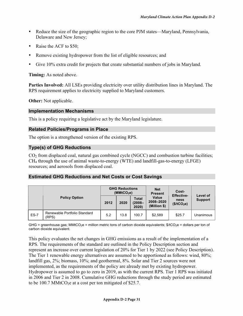
Maryland Climate Action Plan Appendix D-2
Appendix D-2 Page 31
• Reduce the size of the geographic region to the core PJM states—Maryland, Pennsylvania, Delaware and New Jersey;
• Raise the ACF to $50;
• Remove existing hydropower from the list of eligible resources; and
• Give 10% extra credit for projects that create substantial numbers of jobs in Maryland.
Timing: As noted above.
Parties Involved: All LSEs providing electricity over utility distribution lines in Maryland. The RPS requirement applies to electricity supplied to Maryland customers.
Other: Not applicable.
Implementation Mechanisms This is a policy requiring a legislative act by the Maryland legislature.
Related Policies/Programs in Place The option is a strengthened version of the existing RPS.
Type(s) of GHG Reductions CO2 from displaced coal, natural gas combined cycle (NGCC) and combustion turbine facilities; CH4 through the use of animal waste-to-energy (WTE) and landfill-gas-to-energy (LFGE) resources; and aerosols from displaced coal.
Estimated GHG Reductions and Net Costs or Cost Savings
GHG Reductions (MMtCO2e)
Policy Option 2012 2020
Total (2008–2020)
Net Present Value
2008–2020 (Million $)
Cost-Effective-
ness ($/tCO2e)
Level of Support
ES-7 Renewable Portfolio Standard (RPS) 5.2 13.8 100.7 $2,589 $25.7 Unanimous
GHG = greenhouse gas; MMtCO2e = million metric tons of carbon dioxide equivalents; $/tCO2e = dollars per ton of carbon dioxide equivalent. This policy evaluates the net changes in GHG emissions as a result of the implementation of a RPS. The requirements of the standard are outlined in the Policy Description section and represent an increase over current legislation of 20% for Tier 1 by 2022 (see Policy Description). The Tier 1 renewable energy alternatives are assumed to be apportioned as follows: wind, 80%; landfill gas, 2%; biomass, 10%; and geothermal, 8%. Solar and Tier 2 sources were not implemented, as the requirements of the policy are already met by existing hydropower. Hydropower is assumed to go to zero in 2019, as with the current RPS. Tier 1 RPS was initiated in 2006 and Tier 2 in 2008. Cumulative GHG reductions through the study period are estimated to be 100.7 MMtCO2e at a cost per ton mitigated of $25.7.

Maryland Climate Action Plan Appendix D-2
Appendix D-2 Page 32
Maryland has recently updated its RPS to a new standard increasing the requirements for Tier 1 renewables in its portfolio from 9.5% to 20%, which will result in significant GHG reductions over the long term. The difference between the current Maryland RPS and the RPS proposed in this document is the timing of meeting the 20% Tier 1 standard. The current Maryland policy specifies the 20% goal be met by 2022, while the policy proposed in this document sets the date as 2020. The table below provides a quick comparison of previous and current Maryland RPS policies with the RPS policy proposed in this document.
GHG Reductions (MMtCO2e)
Policy Option 2012 2020
Total (2008–2020)
Net Present Value
2008–2020 (Million $)
Cost-Effective-
ness ($/tCO2e)
Level of Support
ES-7 Renewable Portfolio Standard (RPS) 5.2 13.8 100.7 $2,589 $25.7 Unanimous
Previous Maryland RPS 3.0 4.6 48.4 $1,513 $31.2
Current Maryland RPS 4.8 12.2 88.0 $2,329 $26.5
Difference between Current Maryland RPS and RPS proposed in this document
0.4 1.6 12.7 $260.17 $0.8
GHG = greenhouse gas; MMtCO2e = million metric tons of carbon dioxide equivalents; $/tCO2e = dollars per ton of carbon dioxide equivalent.
Data Sources: • Emission projections data come from either CCS inventory and forecast studies of respective
states, or publicly available data from EIA Annual Energy Outlook 2007 for states lacking detailed bottom up assessments.
• R.S. Means. 2007. Heavy Construction Cost Data. Kingston, MA.
• EIA. 2007. Assumptions for the Annual Energy Outlook 2007: with Projections to 2030. Available at http://www.eia.doe.gov/oiaf/aeo/assumption/index.html
• MCCC. 2008. Draft Straw Proposals of Policy Options. Available at http://www.mdclimatechange.us/GHG_Carbon_Mitigation_WG.cfm
• Maryland PPRP. 2006. The Potential for Biomass Co-firing in Maryland. Available at http://esm.versar.com/PPRP/bibliography/PPES_06_02/PPES_06_02.pdf
• Maryland General Assembly (SB 209). 2008. RPS Percentage requirements.
Quantification Methods: Emissions of GHG from coal were compared with GHG emissions from Tier 1 renewables used to replace coal power production. The difference in GHG emissions from coal to renewables is the net GHG reduction for this policy option. Total costs are calculated from levelized NPV costs of power production, adjusted for Maryland construction and fuel costs.

Maryland Climate Action Plan Appendix D-2
Appendix D-2 Page 33
Key Assumptions: Coal is the only power source displaced by Tier 1 renewable energy. The Tier 1 renewable energy alternatives are assumed to be apportioned as follows: wind, 80%; landfill gas, 2%; biomass, 10%; and geothermal, 8%. Solar and Tier 2 sources were not implemented, as the requirements of the policy are already met by existing hydropower. Hydropower is assumed to go to zero in 2019, as with the current RPS. Tier 1 RPS was initiated in 2006 and Tier 2 in 2008.
Key Uncertainties Requirements for 10% extra credit, timing for legislation. The current estimates do not include provisions of subsection (a)(2) from section 7-703 of the RPS standard. Those exclusions will alter the total GHG reductions and associated costs.
Additional Benefits and Costs Reduced air pollution; reduced dependence on fossil fuels.
Feasibility Issues System integration of intermittent power generation; adequacy of electric transmission capacity.
It is likely that there are technical feasibility issues regarding the degree to which biomass co-firing would lead to the risk of wear, corrosion, slagging and fouling in the combustion system.
Status of Group Approval Approved. NOTE: One portion (8b) of this policy is a study product and is presented here for informational purposes.
Level of Group Support Unanimous.
Barriers to Consensus None.

Maryland Climate Action Plan Appendix D-2
Appendix D-2 Page 34
ES-8. Efficiency Improvements and Repowering Existing Plants
Policy Description This policy would promote the identification and pursuit of cost-effective emissions reductions from existing generating units through improving their operating efficiency, adding biomass, or other fuel changes. This policy would complement GPS (which applies to new plants and new units) by addressing existing units. Given that CO2 emissions have not previously been the focus of state regulation, and given that existing units have not been the focus of resource planning, it is expected that there are as-yet unidentified opportunities to reduce emissions from existing facilities that will be cost-effective, particularly once CO2 limits are in place. This policy would, in time, result in the identification of a portfolio of technological options for reducing GHG emissions and allow state utilities to share the opportunities they have identified.
Key aspects of the options include
• Requiring utilities to evaluate their existing generating units for opportunities to improve their emissions profile through efficiency improvements, the addition of biomass or other fuel changes. This evaluation would be part of an overall plan identifying cost-effective options for reducing system CO2 emissions on a short-term and long-term basis.
• Requiring utilities to pursue cost-effective options for reducing their emissions profile through measures identified above.
• Creating financial incentives that reward such emissions reductions. The terms “cost-effective” would be defined by some objective measure, such as cost per ton of carbon equivalent.
The MWG recommends the enactment of planning and emission reduction requirements that are consistent with this Policy Description and Policy Design.
Policy Design Goals: The repowering option should seek to co-fire biomass at existing coal stations at a maximum statewide average rate of 8% of total energy input by 2015. The policy would initiate in 2010 and reach the 8% goal in 2014.
Note: An additional measure was studied in the development of this policy, but was not recommended for adoption by the MWG. The information is retained here as a study product of the MWG. This additional measure is identified as policy “8b” and would set a goal of repowering 30% of eligible coal stations with NG by 2020.
Timing: As noted above.
Parties Involved: The option applies to Maryland electric LSEs.
Other: Not applicable.

Maryland Climate Action Plan Appendix D-2
Appendix D-2 Page 35
Implementation Mechanisms The planning and emission reduction requirements would be implemented through processes already implemented by the Public Utilities Commission (PUC).
Related Policies/Programs in Place The option is an important counterpart to the GPS, which only covers new financial commitments. It complements a C&T policy by ensuring that utilities pursue cost-effective potential emission reductions, rather than the more obvious option of purchasing emission allowances (with the projected price of allowances being a key part of the definition of “cost-effective” reductions).
Type(s) of GHG Reductions All three major GHG emissions (i.e., CO2, CH4, N2O).
Estimated GHG Reductions and Net Costs or Cost Savings
GHG Reductions (MMtCO2e)
Policy Option 2012 2020
Total (2008–2020)
Net Present Value
2008–2020 (Million $)
Cost-Effective-
ness ($/tCO2e)
Level of Support
Efficiency Improvements and Repowering Existing Plants; ES-8a, Biomass Component
1.2 2.0 17.9 $389 $21.8 Unanimous ES-8
ES-8b Repowering Component 0.5 2.9 15.5 $980 $63.2 N/A
GHG = greenhouse gas; MMtCO2e = million metric tons of carbon dioxide equivalents; $/tCO2e = dollars per ton of carbon dioxide equivalent; N/A = not applicable. This policy option evaluates the effect of co-firing biomass in existing coal plants. The biomass portion of the policy assumes that biomass provides 8% of power at existing coal-fired plants. The transition to biomass starts in 2010 and is fully implemented in 2014. The cost associated with biomass is assumed to be $3.40 per million Btu, based on values in a 2006 biomass feasibility report prepared for the State of Maryland, entitled “The Potential for Biomass Co-firing in Maryland” (DNR 12-2242006-107, PPES-06-02).
Total GHG reductions through the study period yield 17.8 MMtCO2e. Biomass is expected to cost about 21.8 $/tCO2e.
The repowering portion of this policy (8b) assumes that by 2020 several coal-powered stations in Maryland are repowered with NGCC technology. In practice, this will be a lumpy process, with steps in GHG reductions achieved as new repowered units come online. For simplicity, the option was modeled as NGCC performance, replacing existing coal performance at a rate of 3% per year, starting in 2011. The conversion of coal plants to NG may reduce the effect of the biomass option. This reduction has not been quantified.

Maryland Climate Action Plan Appendix D-2
Appendix D-2 Page 36
Data Sources: • Emission projections data come from either CCS inventory and forecast studies of respective
states, or publicly available data from EIA Annual Energy Outlook 2007 for states lacking detailed bottom up assessments.
• R.S. Means. 2007. Heavy Construction Cost Data. Kingston, MA.
• EIA. 2007. Assumptions for the Annual Energy Outlook 2007: with Projections to 2030. Available at http://www.eia.doe.gov/oiaf/aeo/assumption/index.html
• MCCC. 2008. Draft Straw Proposals of Policy Options. Available at http://www.mdclimatechange.us/GHG_Carbon_Mitigation_WG.cfm
• Maryland PPRP. 2006. The Potential for Biomass Co-firing in Maryland. Available at http://esm.versar.com/PPRP/bibliography/PPES_06_02/PPES_06_02.pdf
Quantification Methods: Emissions of GHG from coal were compared with emissions from co-fired biomass with the same heating potential. Additionally, coal GHG emissions were compared with GHG emissions from equivalent NGCC power units for the repower portion of this policy option. The difference in emissions from coal to biomass and NGCC is the net GHG reduction for this policy option. Total costs are calculated from levelized NPV costs of power production, adjusted for Maryland construction and fuel costs.
Key Assumptions: Biomass co-firing initiates in 2010 and increases linearly over a 5-year period to a maximum of 8% of energy input at converted plants. This uniform 8% rate is an average. It is recognized that individual coal units will have varying capabilities to cost-effectively accept biomass.
Estimated ‘Warrior Run’ conversion costs are representative of future conversion costs.
Increased demand for biomass does not alter fuel costs.
Conversion from coal to NGCC occurs at a rate of 3% per year, starting in 2010.
Existing coal power is displaced by biomass and NGCC.
The cost associated with biomass is assumed to be $3.40 per million Btu, based on values in a 2006 biomass feasibility report prepared for the State of Maryland, entitled “The Potential for Biomass Co-firing in Maryland” (DNR 12-2242006-107, PPES-06-02).
Key Uncertainties This analysis used a conservative set of assumptions regarding the availability of biomass feedstock within short distances of candidate power plants. The use of this resource for this purpose may compete with other recommendations under considerations by the MWG. These assumptions must be reevaluated if competing uses for this resource are also recommended.
Maryland Climate Action Plan Appendix D-2
Appendix D-2 Page 37
It is unclear how the NSR provisions of the Clean Air Act would affect the promotion of plant upgrades.
Additional Benefits and Costs Reduced air pollution; reduced dependence on fossil fuels.
Feasibility Issues It is likely there are technical feasibility issues regarding the degree to which biomass co-firing would lead to the risk of wear, corrosion, slagging, and fouling in the combustion system.
Status of Group Approval Biomass component (8a) approved. NOTE: The remainder of this policy is a study product and presented here for informational purposes.
Level of Group Support Biomass component - unanimous.
Barriers to Consensus None.
Maryland Climate Action Plan Appendix D-2
Appendix D-2 Page 38
ES-9. Carbon Tax
Policy Description A carbon tax would be a tax on fossil fuels according to the amount of CO2 emitted by their combustion. Carbon tax and C&T systems work toward similar ends in opposite ways. With C&T, the government sets a limit on the tons of pollution that will be released and the market establishes the price. With a carbon tax, the government sets the price and the market drives the level of emissions. The carbon tax and C&T programs are seen as complementary measures. One of the benefits of the tax is it can be more easily applied across all sectors. However, the ES Technical Work Group (TWG) recommends that the C&T program should be the primary market mechanism, with the carbon tax used as a supplementary measure in those sectors where transaction costs or other concerns make the use of C&T less desirable. Like most market-based approaches, it should be applied as broadly as possible, and would be best if applied nationwide.
On the negative side, it is politically difficult to impose a new tax, particularly since other taxes are expected to be rise to cover the Maryland budget deficit. Many economists argue the carbon tax is the most efficient way to ensure that product prices reflect the cost of GHG emissions generated in their manufacture and use. Administrative costs are low for the carbon tax and the impact on prices is predictable. The tax could be imposed upstream based on, for example, the carbon content of fuels (electricity generators or distributors) at the point of combustion and emission or at the point of sale (gasoline, NG). Although taxed entities would pass some or all of the cost on to consumers, there would be competitive pressure to find cost-effective ways to lower (or offset) emissions. Consumers who see the implicit cost of GHG emissions in products and services could adjust their behavior to lower emissions and reduce cost. Revenues collected could offset other taxes, be applied to incentivize low emission alternatives, be directed for relief to parties that are disproportionately impacted by the tax, or rebates could be created for CO2 controls or offsets that prevent atmospheric emissions.
It is assumed that the cost of the tax would be passed down ultimately to the consumer, such as residential and commercial utility ratepayers for electricity. In order to achieve the stated goal, the amount of the tax must be high enough to trigger financial and behavioral decisions toward conservation or a shift to lower emitting fuels.
The MWG does not recommend the enactment of a carbon tax.
Policy Design Goals: Make the cost of inefficient or higher CO2 emitting activities more expensive than alternatives, thereby creating a financial incentive to change behavior away from activities that result in CO2 emissions. The tax should include safety valves to reduce low-income impacts and minimize detrimental economic consequences. One option is to make the tax “revenue neutral,” (an equal amount of other state taxes would be reduced so the “net” to the state is zero). Another option might be that the revenue from the tax could be used to develop or promote alternatives that reduce CO2 emissions. The amount of the tax should be high enough to contribute to the reduction targets specified in the C&T option (see ES-3).

Maryland Climate Action Plan Appendix D-2
Appendix D-2 Page 39
Timing: Pegged to the timing of the C&T option (see ES-3).
Parties Involved: Major payers would be refiners or distributors of transportation and heating fuels in Maryland and commercial and industrial sources consuming energy for production or other commercial use.
Other: The TWG recognizes more in-depth analysis of the carbon tax and its interactions with the C&T and other policies will be required than is possible within the current process. Therefore, it is recommended that a Technical Advisory Committee be convened to study the proposal in greater depth, receive additional public comments, and offer recommendations on the specifics of how a supplemental carbon tax should be enacted and applied.
Implementation Mechanisms This option requires legislation and detailed tax collection system. Specifics of the implementation should be developed through an in-depth investigation as recommended under “Other” above.
Related Policies/Programs in Place The RGGI C&T program and ES-3 are seen as complementary policies.
Type(s) of GHG Reductions Reductions in emissions of CO2 from combustion sources.
Estimated GHG Reductions and Net Costs or Cost Savings As explained in more detail in the Annex, Maryland can meet its state goal by using only negative cost (cost saving) policies and measures. As a result, the incentives for additional GHG mitigation investments provided by a carbon tax are not needed to achieve the goal in principle, because it “pays” emitters to undertake reductions on their own. However, if there is concern about impediments to such voluntary action or if Maryland desired to achieve additional reductions over and above those required by the cap, and possibly through other policies capitalizing on the existence of zero or negative mitigation cost options, a carbon tax could be created offering the following costs and benefits.
Modeling indicates that for each dollar per ton of emissions from non-power sector sources in Maryland, approximately 75,000 tons of CO2e will be mitigated. Assuming the state goal of 25% below 2006 emissions is achieved in 2020, this leaves 48.3 MMtCO2e being emitted from sectors other than the power sector. The implementation of the remaining (unused) negative cost mitigation options beyond the accomplishment of the state goal would reduce the emissions from the non-power sector further from 48.3 to 36.8 MMtCO2e. Therefore, a $1 per ton carbon tax would “cost” $35.5 million (the emitters need to pay $1 tax per every ton of the remaining 36.8 MMtCO2e emissions) and yield 0.1 million tons of reduced emissions, for a cost per ton of $491. This does not take into consideration how the State of Maryland might apply the tax revenues to offset some of this cost.

Maryland Climate Action Plan Appendix D-2
Appendix D-2 Page 40
Data Sources: Emission projections data come from Center for Climate Strategies’ inventory and forecast analysis of Maryland.
Reduction potentials and cost-effectiveness data of mitigation options of Maryland non-power sectors are used to develop the cost curves. This data is provided by other TWGs.
Quantification Methods: The mitigation options list of the non-C&T sectors in Maryland are used in order to evaluate
• Whether the contributions of mitigation options from all the non-C&T sectors would meet the state goal;
• If not, what would be the carbon tax level to non-C&T sectors to achieve the goal; and
• If the mitigation options meet the state goal, how many incremental tons of CO2 will be abated for each incremental dollar of carbon tax.
Some RCI sector options that completely or partially contribute to electricity consumption reduction are included in the options list to develop the Maryland power sector mitigation cost curve used in ES-3. To avoid double counting, the emissions mitigation potential related to electricity consumption reduction of those options are not included in the analysis here.
Key Uncertainties We assume all the negative cost mitigations beyond the state goal would happen without any incentives from a carbon tax. Therefore, for the $1 carbon tax case, the non-power sectors would choose to pay the tax rather than mitigate those emissions that would have a unit reduction cost higher than $1 per ton. However, in practice, it is unclear how much the incentive (the tax rate) should be to encourage all the investments in negative cost opportunities.
Additional Benefits and Costs The availability of $36.8 million in tax revenues per dollar of tax could provide Maryland with a range of additional benefits as a direct result of this policy. Investments in R&D that produce technological breakthroughs might not only produce greater and more cost-effective emissions reductions, but also pay dividends in the form of new jobs and economic growth.
Feasibility Issues Any new tax, even if it is designed to be revenue neutral (revenues offset existing taxes), presents a substantial political challenge, especially in a tight economy. Also, at this point no U.S. state has enacted a carbon tax, so the effort necessary to convince affected groups would be greater than would be the case if there were favorable experience from another U.S. jurisdiction. Administration of the tax would not present particular challenges unless its design included classes of entities that have not previously been subject to similar taxes.

Maryland Climate Action Plan Appendix D-2
Appendix D-2 Page 41
Status of Group Approval This policy is a study product presented here for informational purposes.
Level of Group Support Not applicable.
Barriers to Consensus Not applicable.

Maryland Climate Action Plan Appendix D-2
Appendix D-2 Page 42
ES-10. Generation Performance Standards (GPS)—1,125 Pounds Carbon Dioxide Equivalents per Megawatt-hour (CO2e/MWh)
Policy Description A GPS is a mandate that requires LSEs to acquire electricity on an average portfolio basis, with the portfolio meeting a per-unit emission rate below a specified standard. A GPS portfolio will incentivize investment in new low-carbon generation with overall lower GHG emissions in Maryland. A portfolio approach is a mechanism to control cost to the consumer as well, balancing the ES and environmental goals of the state.
The GPS will be modeled after the existing RPS program, with the exception the GPS may rely on a more diverse mix of replacements for coal power than the RPS. This will help encourage renewable energy sources and will also fit well with any state resource planning process for new generation.
The MWG recommends the enactment of a GPS with a standard of 1125 pounds of GHGs per megawatt-hour (MWh) by 2013.
Policy Design Goals: The general goal of the policy is to encourage the purchase of energy and capacity from low-carbon or renewable technologies. In particular, the GPS portfolio would require that 100% of their energy portfolio emit an average of no more than a specified number of pounds of CO2 per MWh. In response to suggestions made by the MWG, the analysis has been run using three potential GPS standards; 1050, 1100, and 1125 pounds per MWh. The GPS would be designed to harmonize with policies that seek to reduce GHG emissions by promoting greater use of renewable energy sources.
Timing: The program could be implemented by 2013, so as to provide time for new sources to be built.
Parties Involved: The program would apply to any LSE selling energy to retail consumers in the State of Maryland, competitive and those on Standard Offer Service. PSC would need to manage similar to the RPS obligation.
Other: Not applicable.
Implementation Mechanisms Implementation would be through the PUC, which would develop a GPS program similar in design to the current RPS program to ensure compliance with the GPS.
Related Policies/Programs in Place Under ES-7 the current RPS in place in Maryland would be strengthened. The GPS, as proposed here, would be applied separately from the RPS. In other words, the separate requirements of the two standards would not be additive. In addition, ES-8 (Energy Efficiency Improvements and
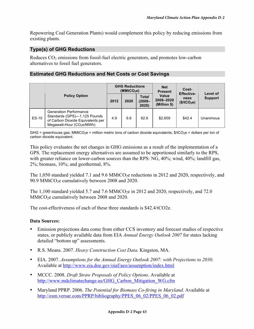
Maryland Climate Action Plan Appendix D-2
Appendix D-2 Page 43
Repowering Coal Generation Plants) would complement this policy by reducing emissions from existing plants.
Type(s) of GHG Reductions Reduces CO2 emissions from fossil-fuel electric generators, and promotes low-carbon alternatives to fossil fuel generators.
Estimated GHG Reductions and Net Costs or Cost Savings
GHG Reductions (MMtCO2e)
Policy Option 2012 2020
Total (2008–2020)
Net Present Value
2008–2020 (Million $)
Cost-Effective-
ness ($/tCO2e)
Level of Support
ES-10
Generation Performance Standards (GPS)—1,125 Pounds of Carbon Dioxide Equivalents per Megawatt-Hour (CO2e/MWh)
4.9 6.6 62.6 $2,659 $42.4 Unanimous
GHG = greenhouse gas; MMtCO2e = million metric tons of carbon dioxide equivalents; $/tCO2e = dollars per ton of carbon dioxide equivalent. This policy evaluates the net changes in GHG emissions as a result of the implementation of a GPS. The replacement energy alternatives are assumed to be apportioned similarly to the RPS, with greater reliance on lower-carbon sources than the RPS: NG, 40%; wind, 40%; landfill gas, 2%; biomass, 10%; and geothermal, 8%.
The 1,050 standard yielded 7.1 and 9.6 MMtCO2e reductions in 2012 and 2020, respectively, and 90.9 MMtCO2e cumulatively between 2008 and 2020.
The 1,100 standard yielded 5.7 and 7.6 MMtCO2e in 2012 and 2020, respectively, and 72.0 MMtCO2e cumulatively between 2008 and 2020.
The cost-effectiveness of each of these three standards is $42.4/tCO2e.
Data Sources: • Emission projections data come from either CCS inventory and forecast studies of respective
states, or publicly available data from EIA Annual Energy Outlook 2007 for states lacking detailed “bottom up” assessments.
• R.S. Means. 2007. Heavy Construction Cost Data. Kingston, MA.
• EIA. 2007. Assumptions for the Annual Energy Outlook 2007: with Projections to 2030. Available at http://www.eia.doe.gov/oiaf/aeo/assumption/index.html
• MCCC. 2008. Draft Straw Proposals of Policy Options. Available at http://www.mdclimatechange.us/GHG_Carbon_Mitigation_WG.cfm
• Maryland PPRP. 2006. The Potential for Biomass Co-firing in Maryland. Available at http://esm.versar.com/PPRP/bibliography/PPES_06_02/PPES_06_02.pdf

Maryland Climate Action Plan Appendix D-2
Appendix D-2 Page 44
Quantification Methods: An analysis of the current electricity mix in Maryland indicates that the average energy intensity is about 1,290 pounds CO2 per MWh. This policy quantifies the effect on GHG of implementing a GPS that stipulates the average emission rate for the entire energy portfolio (in-state and imports) be less than 1,050, 1,100 and 1,125 pounds of CO2 per MWh. GHG emissions and costs from displaced coal were compared with emissions and costs from the mix of replacement power. The differences between these GHG emissions and costs are the net GHG reduction and net cost.
Key Assumptions: This analysis does not consider the emissions associated with the marginal MWh from any one source type or location (i.e., electricity via a dedicated power line from West Virginia). Replacements of existing coal were assumed to be the fixed percentages discussed above. The GPS would be implemented at a rate of 20% per year, starting in 2009, with full implementation occurring in 2013. The GPS, as proposed here, would be applied separately from the RPS. In other words, the separate requirements of the two standards would not be additive.
Key Uncertainties None.
Additional Benefits and Costs Reduced air pollution; increased renewable power produced in Maryland.
Feasibility Issues None.
Status of Group Approval Approved.
Level of Group Support Unanimous.
Barriers to Consensus None.

Maryland Climate Action Plan Appendix D-2
Appendix D-2 Page 45
Annex Analysis of C&T Among Power Sectors
of RGGI States and Carbon Tax in Maryland Non-C&T Sectors in 2020
A. Free Allocation of Allowances The NLP Model used in the study is capable of analyzing various environmental policy instruments, including C&T, carbon taxes, and regulations, under a variety of conditions. For example, for C&T the model can analyze free granting vs. auctioning, upper limits on permit prices, offsets, banking, etc. In some cases, because of the extensive availability of low-cost mitigation options, the supply of allowances in C&T would exceed the demand for allowances at all positive allowance prices. Hence, trading would not be possible (a feasible solution for a positive allowance price that equalizes supply and demand of allowances in the market cannot be obtained from the model). Instead, two scenarios were analyzed with different assumptions for allowance price levels to resolve this problem. Then the supply and demand of allowances from each state, and the costs or savings of individual states before and after entering the C&T system were evaluated.
Example scenario: MC = Allowance Price = $7/tCO2
• According to the initial RGGI allowance allocation, Maryland, Maine, New Hampshire, Vermont, and Rhode Island do not have any GHG mitigation targets, since the allocated allowances to these states (see Column 3 of Table 1) exceed their 2020 BAU emission levels (see Column 2 of Table 1). For the remaining five states, which have binding mitigation goals, the reduction target (%) is computed in Column 4 of Table 1. Next, the reduction potential level was calculated in percentage terms at MC = $7 (see Column 3 of Table 2). If this percentage is lower than the one shown in Column 4 in Table 1, the state would be a buyer of allowances. As shown in Column 4 of Table 2, Connecticut and New Jersey would be the buyers. In total, the allowances demand from these two states is 5.36 MMtCO2. The allowance-selling states would be Delaware, Maryland, Maine, New Hampshire, New York, Vermont, Massachusetts, and Rhode Island.
• After achieving its own reduction target (41.94% below 2020 BAU level), the total allowances available for Delaware to sell with mitigation cost less than $7 are 0.24 MMtCO2. Assuming the remaining RGGI allowance demand (5.36 – 0.24 = 5.12 MMtCO2) would be provided by the other 7 allowance selling states evenly, i.e., each of the selling states would sell 5.12/7 = 0.73 MMtCO2 in the market.
• New York and Massachusetts do not have over-allocated allowances to sell. Therefore, they will provide all of the 0.73 MMtCO2 allowances by autarkic (their own) mitigation actions with costs less than $7/tCO2 (after achieving their own state mitigation targets, these two states still have the capability to reduce emissions with cost less than $7/tCO2). Maryland, Maine, New Hampshire, Rhode Island, and Vermont will decide how much of the allowances they sell would come from autarkic mitigation actions and how much would come from the

Maryland Climate Action Plan Appendix D-2
Appendix D-2 Page 46
excess allowances they possess. To gain the largest profit, these five states would choose to utilize all the cost-saving mitigation potentials inside the state first, since selling these allowances would bring them not only the cost-savings associated with the implementation of the mitigation options, but also the revenues from selling the allowances at the price of $7/tCO2. After exhausting cost-saving mitigation potentials, they will next choose to sell the excess allowances they hold, or undertake mitigation options with zero cost. They can sell these allowances without incurring any mitigation cost. After using up the excess allowances and zero cost options, these five states would be willing to sell those allowances they can achieve through autarkic mitigation actions with costs less than $7/tCO2.
The simulation results of the scenario with allowance price equal to $7/tCO2 are shown in Table 3. Simulation results of the scenario that assumes allowance price to be $1/tCO2 are presented in Table 4. In this case, Delaware would be the third buyer besides Connecticut and New Jersey, since the state autarkic mitigation potentials with MC less than $1 fall short of meeting the state target (though Delaware’s demand of allowance is very small [0.06 MMtCO2e] compared with the other two buyers). Similar simulations were done with assumptions of allowance price at $3/tCO2 and $5/tCO2. These two cases yield similar simulation results as the $7 case, with only Connecticut and New Jersey as the buyers. From the three cases with price at the levels of $3, $5, and $7, the results show a negative relationship between the level of allowance price and the amount of allowances traded among the states. Approximately, allowance transactions are reduced 11 thousand tCO2, with each increased dollar in the allowance price.
Table 1. RGGI States 2020 Emission Projections and Caps
2020 BAU Emissions
(MMtCO2) Cap/Budget (MMtCO2)
Reduction Target
(%)
Allowance Beyond BAU
(MMtCO2)
Reduction Target
(MMtCO2)
CT 13.26 9.09 31.45% 0.00 4.17
DE 11.07 6.43 41.94% 0.00 4.65
MD 31.79 31.88 0.00% 0.09 –0.09
ME 1.90 5.06 0.00% 3.15 –3.15
NH 4.93 7.33 0.00% 2.40 –2.40
NJ 23.40 19.46 16.86% 0.00 3.95
NY 56.11 54.66 2.58% 0.00 1.45
VT 0.03 1.04 0.00% 1.01 –1.01
MA 24.97 22.66 9.26% 0.00 2.31
RI 1.78 2.26 0.00% 0.48 –0.48
Total 169.26 159.87 5.55% 7.13 9.39
BAU = business as usual; MMtCO2 = million metric tons of carbon dioxide.
*The shaded states, Maryland, Maine, New Hampshire, Vermont, and Rhode Island, have allocated allowances higher than their projected 2020 BAU emission levels. As a result, these states have zero emission reduction targets in their power sector. In addition, they can sell the excess allowances in the market at zero mitigation cost.
Sources: 1. RGGI States GHG Caps by Year from 2009 to 2018 are provided by Jeff Wennberg from CCS. Numbers for 2019 and 2020 are estimated by extrapolating 2014 to 2018 numbers.

Maryland Climate Action Plan Appendix D-2
Appendix D-2 Page 47
2. RGGI states 2020 BAU emission projections are obtained from RGGI Web site http://www.rggi.org/documents.htm, the Reference Case projections. The 2020 values are computed by interpolating 2018 and 2021 projections.
Table 2. Determination of Allowances Purchasing and Selling States
Reduction Target
(%)
In-state Reduction Potential with MC<= $7
(%) Whether an
Allowance Buyer Amount of
Allowances to Buy
CT 31.45% 5.78% Yes 3.40
DE 41.94% 44.17% No
MD 0.00% 53.34% No
ME 0.00% 39.92% No
NH 0.00% 6.78% No
NJ 16.86% 8.49% Yes 1.96
NY 2.58% 5.44% No
VT 0.00% 100.00% No
MA 9.26% 47.72% No
RI 0.00% 62.95% No
Total 5.55% 24.71% — 5.36
MC= marginal cost; MC<= $7 (%) = percentage reduction potential with marginal cost less than, or equal to, seven dollars.
Note: If the percentage in the third column is less than the reduction target, in percentage terms, in the second column, the state would be an allowance buyer.
Table 3. Power sector C&T simulation among 10 RGGI states in Year 2020 Scenario 1: allowance price = $7/tCO2 (million dollars or otherwise specified)
Before Trading After Trading
Allowances Traded
Emission Reduction
with Trading
Emission Reduction
Goal
State Mitigation
Cost Mitigation
Cost Trading
Cost Net Cost Cost
Saving (million tCO2)
(million tCO2)
(percent from BAU)
(percent from BAU)
CT 1,200.05 –49.64 23.83 –25.81 1,225.86 3.40 0.77 5.78 31.45
DE –165.12 –164.01 –1.70 –165.71 0.59 –0.24 4.89 44.17 41.94
MD 0.00 –44.41 –5.12 –49.53 49.53 –0.73 0.64 2.02 0.00
ME 0.00 –41.49 –5.12 –46.61 46.61 –0.73 0.72 38.00 0.00
NH 0.00 –25.72 –5.12 –30.84 30.84 –0.73 0.32 6.50 0.00
NJ 38.45 –313.93 13.71 –300.22 338.67 1.96 1.99 8.49 16.86
NY –418.66 –530.22 –5.12 –535.14 116.49 –0.73 2.18 3.88 2.58
VT 0.00 –2.34 –5.12 –7.47 7.47 –0.73 0.03 100.00 0.00
MA –235.68 –301.51 –5.12 –306.63 70.95 –0.73 3.04 12.19 9.26
RI 0.00 –61.48 –5.12 –66.60 66.60 –0.73 1.07 60.45 0.00
Total 419.04 –1,534.55 0.00 –1,534.55 1,953.59 5.36* 15.66 9.25 9.76
tCO2 = tons of carbon dioxide; BAU = business as usual.

Maryland Climate Action Plan Appendix D-2
Appendix D-2 Page 48
*Represents number of allowances bought or sold.
Table 4. Power sector C&T simulation among 10 RGGI states in Year 2020 Scenario 2: allowance price = $1/tCO2 (million dollars or otherwise specified)
Before Trading After Trading
Allowances Traded
Emission Reduction
with Trading
Emission Reduction
Goal
State Mitigation
Cost Mitigation
Cost Trading
Cost Net Cost Cost
Saving (million tCO2)
(million tCO2)
(percent from BAU)
(percent from BAU)
CT 1,200.05 –49.77 3.44 –46.33 1,246.38 3.44 0.73 5.54 31.45
DE –165.12 –165.20 0.06 –165.15 0.02 0.06 4.59 41.46 41.94
MD 0.00 –47.96 –0.78 –48.75 48.75 –0.78 0.69 2.19 0.00
ME 0.00 –41.49 –0.78 –42.27 42.27 –0.78 0.72 38.00 0.00
NH 0.00 –25.72 –0.78 –26.50 26.50 –0.78 0.32 6.50 0.00
NJ 38.45 –314.07 1.99 –312.07 350.52 1.99 1.95 8.34 16.86
NY –418.66 –535.37 –0.78 –536.15 117.49 –0.78 2.23 3.98 2.58
VT 0.00 –2.34 –0.78 –3.13 3.13 –0.78 0.03 100.00 0.00
MA –235.68 –306.05 –0.78 –306.83 71.15 –0.78 3.10 12.40 9.26
RI 0.00 –61.48 –0.78 –62.26 62.26 –0.78 1.07 60.45 0.00
Total 419.04 –1,549.45 0.00 –1,549.45 1,968.48 5.49* 15.45 9.13 9.76
tCO2 = tons of carbon dioxide; BAU = business as usual.
*Represents number of allowances bought or sold.
B. Auction of Allowances In the case where allowances are auctioned, the 2020 emission caps for Connecticut, Delaware, New Jersey, New York, and Massachusetts were assumed to be the same as in the free granting case. For Maryland, Maine, New Hampshire, Vermont, and Rhode Island, which have excess allowances in the free granting case, it was assumed their caps in the auction case would equal the state BAU 2020 emission levels (i.e., there is no reason to purchase any excess allowances at auction). Table 5 shows the emission caps for the 10 RGGI states in the auction case.

Maryland Climate Action Plan Appendix D-2
Appendix D-2 Page 49
Table 5. RGGI States 2020 Emission Projections and Caps (Auction Case)
2020 BAU Emissions (MMtCO2)
Cap/Budget (MMtCO2)
CT 13.26 9.09
DE 11.07 6.43
MD 31.79 31.79
ME 1.90 1.90
NH 4.93 4.93
NJ 23.40 19.46
NY 56.11 54.66
VT 0.03 0.03
MA 24.97 22.66
RI 1.78 1.78
Total 169.26 152.82
BAU = business as usual; MMtCO2 = million metric tons of carbon dioxide. In the auction case, there would be no trading among states. According to the basic rationale for permit trading, in equilibrium, each state would choose to mitigate emissions, as long as its marginal abatement cost is lower than or equal to the price of allowances, and purchase the remaining allowance (the difference between the state’s BAU level and the amount mitigated by autarkic actions) from the auctioneer. Table 6 presents the amount of emissions that can be reduced by each state’s autarkic mitigation actions associated with MC of $7/tCO2e. The simulation results of the auction case with allowance price equal to $7/tCO2e are presented in Table 7. A second simulation with the auction price assumed to be at $1/tCO2e is presented in Table 8.
In usual C&T cases, where the equilibrium point corresponds to a positive allowance price, auction and free granting would reach the same cost-effectiveness level, i.e., the auction price would be at the same level as the equilibrium price in the allowance trading market, and the collaborative CO2 reductions achieved by the partner states in these two allocation cases would be the same and equal to the overall emission reduction target of the region. The only difference between these two allocation cases would be that the auction can generate revenues to the state government, which in turn can be recycled to fund R&D in such innovations as clean energy technologies and end-use energy efficiencies, and thus, lower the impacts to the electricity ratepayers.
However, as indicated in Section A, the supply would exceed the demand at all positive allowance prices in RGGI’s case. Therefore, in the case of C&T with a grandfathering allocation strategy and with the assumed market price at $7/tCO2, to ensure the balance of trade in the market (supply equalizing demand), many states (e.g., Maryland, New York, Massachusetts) would not use up all their mitigation potentials with MC less than $7/tCO2. Collaboratively, the emission reductions achieved by the 10 states in the free granting case with allowance price equal to $7/tCO2 are 15.66 MMtCO2. Beyond C&T, a state would still be willing to mitigate any ton of GHG that would bring net cost savings. The additional cost-saving mitigation potential for

Maryland Climate Action Plan Appendix D-2
Appendix D-2 Page 50
the 10 states beyond C&T (free granting case) is 24.00 MMtCO2. In the auction case, each state would utilize all its mitigation potential with MC less than $7/tCO2 before purchasing allowances from the auctioneer. As a result, the total emission reductions achieved by the 10 states in this case are 41.82 MMtCO2. Since considerable amounts of unused mitigation potentials of some states (e.g., Maryland, Massachusetts) in the free granting case are associated with cost savings, the total cost savings of mitigation in the auction case (2.54 billion) are higher than the total mitigation cost savings in the free granting case (1.53 billion). In addition, in the auction case many states would reduce more emissions than required by the state mitigation target (because it is cheaper to mitigate than to buy from the auctioneer). The additional reductions achieved by these states can be saved for future use.
Comparing the two auction cases with auction prices at $7 and $1, the amount the states choose to reduce by mitigation options (41.82 MMtCO2 vs. 39.98 MMtCO2) and the amount to be bought from the auctioneer (127.44 MMtCO2 vs. 129.28 MMtCO2) differ slightly. The big difference in total auction cost between these two cases is due primarily to the difference of the two auction price levels.
Table 6. Mitigation potential associated with MC = $7/tCO2e
Cap/Budget (MMtCO2)
In-state Reduction
Potential with MC<= $7
(%)
In-state Reduction
Potential with MC<= $7 (MMtCO2)
CT 9.09 5.78% 0.77
DE 6.43 44.17% 4.89
MD 31.88 53.34% 16.96
ME 1.90 39.92% 0.76
NH 4.93 6.78% 0.33
NJ 19.46 8.49% 1.99
NY 54.66 5.44% 3.05
VT 0.03 100.00% 0.03
MA 22.66 47.72% 11.92
RI 1.78 62.95% 1.12 Total 152.82 24.71% 41.82
MMtCO2 = million metric tons of carbon dioxide; MC<= $7 = marginal cost is less than or equal to seven dollars.

Maryland Climate Action Plan Appendix D-2
Appendix D-2 Page 51
Table 7. Simulation results of an auction case among RGGI states (with assumed auction price at $7/tCO2)
Emission Reduction
Undertaken by the State*
State
Total BAU Emissions
in 2020 (million tCO2)
2020 Emissions
Cap/Budget (million tCO2)
(percent from BAU)
(million tCO2)
Mitigation Cost
(million $)
Emission Allowances Bought from Auctioneer
(million tCO2)
Auction Cost
(million $)† Net Cost
(million $)‡ CT 13.26 9.09 5.78 0.77 –49.64 12.50 87.47 37.83
DE 11.07 6.43 44.17 4.89 –164.01 6.18 43.28 –120.73 MD 31.79 31.88 53.34 16.96 –617.74 14.83 103.83 –513.91
ME 1.90 1.90 39.92 0.76 –41.36 1.14 8.00 –33.36
NH 4.93 4.93 6.78 0.33 –25.67 4.59 32.16 6.48
NJ 23.40 19.46 8.49 1.99 –313.93 21.42 149.92 –164.01
NY 56.11 54.66 5.44 3.05 –573.12 53.06 371.43 –201.69
VT 0.03 0.03 100.00 0.03 –2.34 0.00 0.00 –2.34
MA 24.97 22.66 47.72 11.92 –692.28 13.06 91.40 –600.88
RI 1.78 1.78 62.95 1.12 –61.32 0.66 4.61 –56.71 Total 169.26 152.82 24.71 41.82 –2,541.43 127.44 892.09 –1,649.33
BAU = business as usual; tCO2 = tons of carbon dioxide.
* In equilibrium, each state will choose to mitigate to the level that its marginal abatement cost equals the auction price.
† We assume the auction price is $7/tCO2 in this case.
‡ Sum of mitigation cost and auction cost.

Maryland Climate Action Plan Appendix D-2
Appendix D-2 Page 52
Table 8. Simulation results of an auction case among RGGI states (with assumed auction price at $1/tCO2)
Emission Reduction
Undertaken by the State*
State
Total BAU Emissions
in 2020 (million tCO2)
2020 Emissions
Cap/Budget (million tCO2)
(percent from BAU)
(million tCO2)
Mitigation Cost
(million $)
Emission Allowances Bought from Auctioneer
(million tCO2)
Auction Cost
(million $)† Net Cost
(million $)‡ CT 13.26 9.09 5.54 0.73 –$49.77 12.53 $12.53 –$37.24
DE 11.07 6.43 41.46 4.59 –$165.20 6.48 $6.48 –$158.72 MD 31.79 31.88 50.49 16.05 –$620.34 15.74 $15.74 –$605.60
ME 1.90 1.90 38.28 0.73 –$41.49 1.17 $1.17 –$40.31
NH 4.93 4.93 6.54 0.32 –$25.72 4.61 $4.61 –$21.11
NJ 23.40 19.46 8.34 1.95 –$314.07 21.45 $21.45 –$292.62
NY 56.11 54.66 5.35 3.00 –$573.31 53.11 $53.11 –$520.20
VT 0.03 0.03 100.00 0.03 –$2.34 0.00 $0.00 –$2.34
MA 24.97 22.66 45.96 11.48 –$694.03 13.50 $13.50 –$680.54
RI 1.78 1.78 60.81 1.08 –$61.47 0.70 $0.70 –$60.78 Total 169.26 152.82 23.62 39.98 –$2,548.74 129.28 $129.28 –$2,419.46
BAU = business as usual; tCO2 = metric tons of carbon dioxide.
* In equilibrium, each state will choose to mitigate to the level that its marginal abatement cost equals the auction price.
† In this case, it is assumed that the auction price is $1/tCO2.
‡ Sum of mitigation cost and auction cost.
Development of the Marginal Cost Curves of Power Sector The MC curves of the states are developed based on the reduction potential and mitigation cost/saving data of individual options that contribute to the emission reductions from power sector. These options not only include those designed directly for the electricity supply sector (e.g., promotion of renewable energy utilization, repowering existing plants, GPS), but also include options in RCI sectors that contribute to the reduction of electricity consumption (e.g., DSM, energy efficient appliances, building codes). The emission reduction potentials of these options are adjusted by multiplying the percentage of electricity consumption to total energy consumption in the RCI sector. RCI options that relate entirely to reduction of other fossil fuels consumption (e.g., gas, oil) are not included in the cost curve development. Table 9 presents the list of options of Maryland used to develop the MC curve of the state.

Maryland Climate Action Plan Appendix D-2
Appendix D-2 Page 53
Table 9. Maryland Mitigation options list to develop the MC curve of power sector
Sector Climate Mitigation Actions
Estimated 2020
Annual GHG
Reduction Potential
(MMtCO2e)
Estimated Cost or
Cost Savings per ton
GHG Removed
GHG Reduction
Potential as Percentage
of 2020 Baseline
Emissions*
Cumulative GHG
Reduction Potential
Weights (add up to 100)
RCI-7 More Stringent Appliance / Equipment Efficiency Standards (State-Level, or Advocate for Regional- or Federal-Level Standards)
0.14 –$54.00 0.42% 0.42% 0.329
RCI-4 Improved Design, Construction, Appliances, and Lighting in New and Existing State and Local Government Buildings, “Government Lead-By-Example”
0.89 –$53.00 2.80% 3.22% 2.167
RCI-10 Energy Efficiency Resource Standard (EERS)
8.04 –$52.00 25.28% 28.50% 19.592
RCI-2 Demand-Side Management (DSM) / Energy Efficiency Programs, Funds, or Goals for Electricity (Including Expansion of Existing Programs and Peak Load Reduction)
3.70 –$51.00 11.64% 40.14% 9.021
RCI-11 Promotion and Incentives for Energy-Efficient Lighting
1.10 –$47.00 3.46% 43.60% 2.682
RCI-3 Low-Cost Loans for Energy Efficiency
0.35 –$45.00 1.09% 44.69% 0.847
RCI-1 Improved Building and Trade Codes and Beyond-Code Building Design and Construction
1.67 –$38.00 5.25% 49.94% 4.067
ES-5b Clean Distributed Generation (DG): Combined Heat and Power (CHP)
1.00 $14.40 3.15% 53.08% 2.438
ES-8a Efficiency Improvements and Repowering Existing Plants—Distributed Generation (DG)
2.00 $21.80 6.29% 59.37% 4.876
ES-7 Renewable or Environmental Portfolio Standard (e.g., Add CHP or EE To RPS as Additional Tier) or Energy Efficiency Portfolio Standard
13.80 $25.70 43.41% 102.79% 33.647
ES-1 Promotion of Renewable Energy (Zoning, Siting, Incentives for Centralized Facilities, Long-Term Contracting, Performance-Based Contracting)
0.50 $27.00 1.57% 104.36% 1.219
ES-5a Clean Distributed Generation (DG): Distributed Generation
1.10 $37.50 3.46% 107.82% 2.682

Maryland Climate Action Plan Appendix D-2
Appendix D-2 Page 54
Sector Climate Mitigation Actions
Estimated 2020
Annual GHG
Reduction Potential
(MMtCO2e)
Estimated Cost or
Cost Savings per ton
GHG Removed
GHG Reduction
Potential as Percentage
of 2020 Baseline
Emissions*
Cumulative GHG
Reduction Potential
Weights (add up to 100)
ES-10 Generation Performance Standards (GPS)—1,125 Pounds Carbon Dioxide Equivalents per Megawatt-Hour (Co2e/MWh)
6.60 $42.40 20.76% 128.58% 16.092
RCI-8 Rate Structures and Technologies to Promote Reduced Greenhouse Gas (GHG) Emissions (Including Peak Pricing and Inverted Block Rates)
0.14 $120.00 0.44% 129.02% 0.339
GHG = greenhouse gas; MMtCO2e = million metric tons of carbon dioxide equivalents; EE = energy efficiency; RPS = renewable portfolio standard; CCSR = combined capture, storage, and reuse.
* 2020 projected production-based gross emission level is 31.79 MMtCO2e. In Table 9, Column 3 presents the estimated 2020 annual GHG reduction potential for each relevant option, with reduction potentials translated into percentages of the 2020 ES BAU emissions level in Column 5. The estimated cost or cost saving per ton of GHG removed by each option in 2020 is presented in Column 4. The options are ordered in ascending sequence in terms of cost, beginning with the cheapest option. Column 6 calculates the cumulative GHG reduction potentials of the first n policy options listed in the table. The last column presents the proportion of GHG mitigation contributed by each option.
Based on the data presented in Table 9, the stepwise MC function for Maryland in 2020 is drawn in Figure 1. The horizontal axis represents the percentage of GHG emissions reduction, and the vertical axis represents the MC or savings of mitigation. In the figure, each horizontal segment represents an individual mitigation option. The width of the segment indicates the GHG emission reduction potential of the option in percentage terms. The height of the segment relative to the x-axis shows the average cost (saving) of reducing 1 ton of GHG with the application of the option.
Next, the following functional form was used to fit the smooth Maryland MC curve to be used in our analysis:
Where, MC is the marginal cost; R is the percentage reduction of GHG emissions; a and b are parameters.
The logarithmic functional form utilized here is consistent with theoretical expectations and empirical findings on diminishing returns of emission control. As the emission reductions increase along the x-axis, the cost to reduce one additional unit of emission is increasing at an accelerating speed.

Maryland Climate Action Plan Appendix D-2
Appendix D-2 Page 55
To develop the fitted cost curve, it is forced to cross the x-axis through the point of 50%, the same x-intercept indicated by the step function. The MC curve of Maryland has the following specification:
Figure 1 shows the step and fitted MC curves of the Maryland power sector.
Figure 1. MC curves of Maryland power sector
$/tCO2e = dollars per metric ton of carbon dioxide equivalent; BAU = business as usual; GHG = greenhouse gas.

Maryland Climate Action Plan Appendix D-2
Appendix D-2 Page 56
Figure 2. State MC curves of power sector, 2020
$/tCO2e = dollars per metric ton of carbon dioxide equivalent; RGGI = Regional Greenhouse Gas Initiative; GHG = greenhouse gas; MD = Maryland; ME = Maine; RI = Rhode Island; CT = Connecticut; NY = New York; MA = Massachusetts; NJ = New Jersey; NH = New Hampshire; DE = Delaware; VT = Vermont.
Notes: Similar methods as elaborated above for Maryland are adopted to develop MC curves of Connecticut, Maine, New York, Rhode Island, and Vermont. Data sources are listed below.
There are no direct data for Massachusetts, New Jersey, New Hampshire, and Delaware. MC curves for these four states are developed based on cost curves of four reference states (Rhode Island, New York, Connecticut, and Maryland, respectively). For each of the four states that lack the direct data, mitigation cost/saving data for the reference state is adopted. Emission reduction potential data of the reference state is adjusted by the weights of emissions from the ES and RCI sectors of the state under estimation.
Sources: • Connecticut GSC on Climate Change. 2005. 2005 CT Climate Change Action Plan. Available at
http://www.ctclimatechange.com/StateActionPlan.html • MCCC. 2008. Maryland Climate Change Action Plan. Available at http://www.mdclimatechange.us/index.cfm • Maine DEP. 2004. Final Maine Climate Action Plan 2004. Available at http://www.maine.gov/dep/air/greenhouse/ • CCAP and New York GHG Task Force. 2003. Recommendations to Governor Pataki for Reducing New York
State Greenhouse Gas Emissions. Available at http://www.ccap.org/pdf/04-2003_NYGHG_Recommendations.pdf • RI GHG. 2002. Rhode Island Greenhouse Gas Action Plan. Available at http://righg.raabassociates.org/. • Vermont GCCC. 2007. Final Report and Recommendations of the Governor’s Commission on Climate Change.
Available at http://www.anr.state.vt.us/air/Planning/htm/ClimateChange.htm.
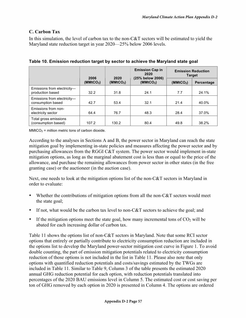
Maryland Climate Action Plan Appendix D-2
Appendix D-2 Page 57
C. Carbon Tax In this simulation, the level of carbon tax to the non-C&T sectors will be estimated to yield the Maryland state reduction target in year 2020—25% below 2006 levels.
Table 10. Emission reduction target by sector to achieve the Maryland state goal
Emission Reduction Target
2006
(MMtCO2) 2020
(MMtCO2)
Emission Cap in 2020
(25% below 2006) (MMtCO2) (MMtCO2) Percentage
Emissions from electricity—production based 32.2 31.8 24.1 7.7 24.1%
Emissions from electricity—consumption based 42.7 53.4 32.1 21.4 40.0%
Emissions from non-electricity sector 64.4 76.7 48.3 28.4 37.0%
Total gross emissions (consumption based) 107.2 130.2 80.4 49.8 38.2%
MMtCO2 = million metric tons of carbon dioxide. According to the analyses in Sections A and B, the power sector in Maryland can reach the state mitigation goal by implementing in-state policies and measures affecting the power sector and by purchasing allowances from the RGGI C&T system. The power sector would implement in-state mitigation options, as long as the marginal abatement cost is less than or equal to the price of the allowance, and purchase the remaining allowances from power sector in other states (in the free granting case) or the auctioneer (in the auction case).
Next, one needs to look at the mitigation options list of the non-C&T sectors in Maryland in order to evaluate:
• Whether the contributions of mitigation options from all the non-C&T sectors would meet the state goal;
• If not, what would be the carbon tax level to non-C&T sectors to achieve the goal; and
• If the mitigation options meet the state goal, how many incremental tons of CO2 will be abated for each increasing dollar of carbon tax.
Table 11 shows the options list of non-C&T sectors in Maryland. Note that some RCI sector options that entirely or partially contribute to electricity consumption reduction are included in the options list to develop the Maryland power-sector mitigation cost curve in Figure 1. To avoid double counting, the part of emission mitigation potentials related to electricity consumption reduction of those options is not included in the list in Table 11. Please also note that only options with quantified reduction potentials and costs/savings estimated by the TWGs are included in Table 11. Similar to Table 9, Column 3 of the table presents the estimated 2020 annual GHG reduction potential for each option, with reduction potentials translated into percentages of the 2020 BAU emissions level in Column 5. The estimated cost or cost saving per ton of GHG removed by each option in 2020 is presented in Column 4. The options are ordered

Maryland Climate Action Plan Appendix D-2
Appendix D-2 Page 58
in ascending sequence in terms of cost, beginning with the cheapest option. Column 6 calculates the cumulative GHG reduction potentials of the first n policy options listed in the table. The last column presents the proportion of GHG mitigation contributed by each option.
Table 11. Mitigation options list of non-C&T sectors in Maryland
Sector Climate Mitigation Actions
Estimated 2020 Annual
GHG Reduction Potential
(MMtCO2e)
Estimated Cost or Cost Savings per
Ton GHG Removed
GHG Reduction
Potential as Percentage of 2020 Baseline Emissions†
Cumulative GHG
Reduction Potential
AFW-5 “Buy Local” Programs for Sustainable Agriculture, Wood, and Wood Products—a. Farmer’s Market
0.03 –$167.00 0.04% 0.04%
AFW-2
Managing Urban Trees and Forests for Greenhouse Gas (GHG) Benefits (With Mitigation of Forest Loss Due to Insects, Disease, Pests, and Invasive Species)
1.90 –$152.00 2.48% 2.52%
RCI-7
More Stringent Appliance / Equipment Efficiency Standards (State-Level, or Advocate for Regional- or Federal-Level Standards)
0.06 –$54.00 0.08% 2.60%
RCI-4
Improved Design, Construction, Appliances, and Lighting in New and Existing State and Local Government Buildings, “Government Lead-by-Example”
0.41 –$53.00 0.54% 3.14%
RCI-10 Energy Efficiency Resource Standard (EERS) 3.86 –$52.00 5.04% 8.18%
RCI-3 Low-Cost Loans for Energy Efficiency 0.15 –$45.00 0.20% 8.37%
RCI-1 Improved Building and Trade Codes and Beyond-Code Building Design and Construction
0.73 –$38.00 0.95% 9.33%
AFW-8 Nutrient Trading With Carbon Benefits 0.14 $30.00 0.18% 9.51%
AFW-9 Waste Management Through Source Reduction and Advanced Recycling 29.20 –$6.00 38.06% 47.57%
AFW-6
Expanded Use of Forest and Farm Feedstocks and By-Products for Energy Production—Methane (CH4) Utilization From Livestock Manure and Poultry Litter
0.04 $0.20 0.05% 47.62%
AFW-7 In-State Liquid Biofuels Production—Bio-diesel 0.17 $7.00 0.22% 47.84%
AFW-6
Expanded Use of Forest and Farm Feedstocks and By-Products for Energy Production—Biomass (Including Agriculture Residue, Forest Feedstocks, and Energy Crops)
0.50 $12.00 0.65% 48.29%
AFW-3 Afforestation, Reforestation, and Restoration of Forests and Wetlands—
0.60 $29.00 0.78% 49.28%

Maryland Climate Action Plan Appendix D-2
Appendix D-2 Page 59
Sector Climate Mitigation Actions
Estimated 2020 Annual
GHG Reduction Potential
(MMtCO2e)
Estimated Cost or Cost Savings per
Ton GHG Removed
GHG Reduction
Potential as Percentage of 2020 Baseline Emissions†
Cumulative GHG
Reduction Potential
a. Afforestation
AFW-4 Forested Land— b. Forested Land 2.70 $37.00 3.52% 52.79%
AFW-3 Afforestation, Reforestation, and Restoration of Forests and Wetlands— b. Riparian Areas
0.05 $44.00 0.07% 52.86%
TLU-4* Low Greenhouse Gas Fuel Standard (LGFS) 1.90 $60.00 2.48% 55.34%
AFW-7 In-State Liquid Biofuels Production—Ethanol 0.91 $80.00 1.19% 56.52%
AFW-4 Forested Land— a. Agricultural Land 0.28 $87.00 0.36% 56.89%
RCI-8 Rate Structures and Technologies To Promote Reduced GHG Emissions (Including Inverted Block Rates)
0.06 $120.00 0.08% 56.97%
AFW-1
Forest Management for Enhanced Carbon Sequestration (With Mitigation of Forest Loss Due to Insects, Disease, Pests, and Invasive Species)
0.09 $135.00 0.12% 57.08%
TLU-10* Transportation Technologies 0.44 $650.00 0.57% 57.66%
GHG = greenhouse gas; MMtCO2e = million metric tons of carbon dioxide equivalents.
* Numbers presented in the column of “Estimated Cost or Cost Savings per Ton GHG Removed” are the average of the high and low estimates by the TLU TWG.
† 2020 projected gross CO2 emissions from non-C&T sectors are 76.92 MMtCO2e. From Column 6 of Table 11, the cumulative mitigation potential of options with cost savings is around 47.57% of the non-C&T sectors’ 2020 BAU emissions level. As shown in Table 10, the reduction goal of 25% below the 2006 level translates to 37.0% below 2020 BAU level for the non-C&T sectors. Therefore, the state goal can be over-achieved by implementing only the cost-saving mitigation options.
Thus, to achieve current 2020 goal, the carbon tax is not needed. However, one can examine the potential of a carbon tax for additional mitigation in the following way. Fit a smooth curve through the points of options with unit mitigation cost higher than zero (see the smooth curve in Figure 3). Based on the curve, Table 12 presents the total reduction potentials of the non-C&T sectors with assumed carbon tax levels at $1 to $7. Approximately, for every $1 increase in the carbon tax, an additional 75 thousand tons of CO2 will be abated in the non-C&T sectors.

Maryland Climate Action Plan Appendix D-2
Appendix D-2 Page 60
Figure 3. MC curve of non-C&T sectors in Maryland
$/tCO2e = dollars per metric ton of carbon dioxide equivalent C&T = cap-and-trade; MD = Maryland; BAU = business as usual; GHG = greenhouse gas.
Note: The step curve is developed based on the options data in Table 11. The horizontal axis represents the percentage of GHG emissions reduction, and the vertical axis represents the MC or savings of mitigation. In the figure, each horizontal segment represents an individual mitigation option. The width of the segment indicates the GHG emission reduction potential of the option in percentage terms. The height of the segment relative to the x-axis shows the average cost (saving) of reducing 1 ton of GHG with the application of the option. The smooth curve is fitted through the points of options with unit mitigation cost higher than zero.
Table 12. Carbon tax level and corresponding total reduction potential in non-C&T sectors
Total Reduction Potential
Carbon Tax ($/tCO2)
% 2020 BAU level MMtCO2
Incremental Reduction per Dollar Increase in
the Carbon Tax (thousand tCO2)
0 48.02% 36.84
1 48.12% 36.92 75.57
2 48.22% 36.99 75.43
3 48.31% 37.07 75.28
4 48.41% 37.15 75.14
5 48.51% 37.22 75.00
6 48.61% 37.29 74.86
7 48.70% 37.37 74.71
$/tCO2 = dollars per ton of carbon dioxide; BAU = business as usual; MMtCO2 = million metric tons of carbon dioxide.

Maryland Climate Action Plan
Appendix D-3
Residential, Commercial & Industrial

Maryland Climate Action Plan Appendix D-3
Appendix D-3 Page 2
Residential, Commercial, and Industrial Sector
Summary List of Recommended Priority Policy Options for Analysis
GHG Reductions (MMtCO2e)
Option No. Policy Option
2012 2020 Total 2008– 2020
Net Present Value 2008–2020
(Million $)
Cost-Effective-
ness ($/tCO2e)
Level of Support
RCI-1 Improved Building and Trade Codes and Beyond-Code Building Design and Construction in the Private Sector
0.6 2.4 13.8 –$527 –$38 Unanimous
RCI-2
Demand-Side Management (DSM) / Energy Efficiency Programs, Funds, or Goals for Electricity and Natural Gas (Including Expansion of Existing Programs and Peak Load Reduction)
1.8 4.5 35.0 –$1,898 –$54 Unanimous
RCI-3 Low-Cost Loans for Energy Efficiency 0.3 0.5 4.1 –$187 –$45 Unanimous
RCI-4
Improved Design, Construction, Appliances, and Lighting in New and Existing State and Local Government Buildings, Facilities and Operations: “Government Lead-by-Example”
0.2 1.3 6.4 –$337 –$53 Unanimous
RCI-5 Energy Efficiency and Environmental Impacts Awareness and Instruction in School Curricula
Jointly considered with the CC TWG Unanimous
RCI-6
Promotion and Incentives for Improved Design and Construction (e.g., LEED™, Green Buildings, or Minimum Percent Improvement Better Than Code) in the Private Sector
Combined with RCI-1
RCI-7
More Stringent Appliance / Equipment Efficiency Standards (State-Level, or Advocate for Regional- or Federal-Level Standards)
0.1 0.2 1.2 –$63 –$54 Unanimous
RCI-8 Rate Structures and Technologies To Promote Reduced GHG Emissions (Including Peak Pricing and Inverted Block Rates)
0.1 0.2 2.0 $246 $120 Unanimous
RCI-9 GHG or Carbon Tax Transferred to ES TWG
RCI-10 Energy Efficiency Resource Standard (EERS) 2.9 11.9 71.0 –$3,670 –$52 Unanimous
RCI-11 Promotion and Incentives for Energy Efficient Lighting 0.1 1.1 7.7 –$362 –$47 Unanimous
Sector Total After Adjusting for Overlaps* 1.1 11.2 54.1 –$5,450 –$48 Reductions From Recent Actions† 4.3 9.0 71.5 Not quantified
Sector Total Plus Recent Actions 5.4 20.2 125.5 Not quantified
GHG = greenhouse gas; MMtCO2e = million metric tons of carbon dioxide equivalent; $/tCO2e = dollars per metric ton of carbon dioxide equivalent.
* These totals account for the interaction between RCI policies. The benefits and costs of RCI policies overlap as follows: between residential and commercial new construction in RCI-1, RCI-2, and RCI-10; between RCI–4 and energy efficiency efforts in government and schools within RCI-2 and RCI-10; between RCI-7 and parts of RCI-2,

Maryland Climate Action Plan Appendix D-3
Appendix D-3 Page 3
RCI-4, and RCI-10; and between RCI-11 and parts of RCI-2, RCI-4, and RCI-10. Overlaps also occur between RCI and Energy Supply (ES), to the extent that demand is reduced by RCI measures, and generation emits less GHGs after ES policies; adjustments for overlaps between RCI and ES are quantified in the ES cumulative analysis. An overlap with Agriculture, Forestry, and Waste Management-2 (AFW-2) has been quantified in the AFW cumulative analysis.
† Recent actions include the Energy Independence and Security Act of 2007 Title III (Appliance and Lighting Efficiency), Maryland Energy Efficiency Standards Act of 2007, and EmPOWER MD (HB 374).
Note: The numbering used to denote the above policy options is for reference purpose only; it does not reflect prioritization among these important policy options.
The following policy recommendations reflect consensus positions of the RCI Technical Work Group (TWG) and do not necessarily represent the views of the individual members.

Maryland Climate Action Plan Appendix D-3
Appendix D-3 Page 4
RCI-1. Improved Building and Trade Codes and Beyond-Code Building Design and Construction in the Private Sector
Policy Description Buildings are significant consumers of energy and other resources, and can contribute to local microclimates. According to the Environmental Protection Agency (EPA), December 2004, in the United States buildings account for 39% of the total energy use, 12% of the water consumption, 68% of the electricity consumption, and 38% of the total carbon dioxide emissions. Given the long lifetime of most buildings, amending state and/or local building codes to include minimum energy efficiency requirements and periodically updating energy efficiency codes could provide long-term GHG savings.
This policy sets a goal for reducing building energy consumption, to be achieved by increasing standards for the minimum performance of new and substantially renovated commercial and residential buildings through the adoption and enforcement of building and trade codes. Building codes would be made more stringent via incorporation of aspects of advanced/next generation building designs and construction standards, such as Leadership in Energy and Environmental Design Green Building Rating System™ (LEED) or a comparable standard. Other aspects of the policy design include:
• Undertaking a comprehensive review of existing State and local building and trades codes in Maryland to determine where increased energy efficiency can be achieved.
• Developing a training and certification program for code officials, builders, and contractors on energy efficiency and related Green building and trade codes, and in code enforcement.
• Providing tools to state and local governments for measurement and tracking of cost savings. • Incorporating future code upgrades by reference language in the statute or regulation to avoid
having to re-open the rule each time the referenced body changes its code. • Targeting existing buildings for efficiency improvements during both major and minor
renovation, through application and enforcement of building codes and/or with tax rebates or other incentives.
• Encouraging or requiring continued high performance of buildings that receive tax rebates or other incentives, through participation in LEED for Existing Buildings (LEED-EB) or comparable standard.
• Allowing compliance flexibility. New and substantially renovated buildings can utilize a combination of increased energy efficiency, switching to low and no carbon-based fuels for previously carbon-based end-uses, off-site purchases on grid supplied “green power” and/or installing on-site off-grid power generating equipment.
• Establishing specific goals for the size of building to be included, e.g., using Montgomery County Bill 17-06 as a model.
• Setting a cap on consumption of energy per unit area of floor space for new buildings.

Maryland Climate Action Plan Appendix D-3
Appendix D-3 Page 5
• Requiring high-efficiency appliances in new construction and retrofits. • Providing incentives, such as permitting and fee advantages, tax credits, financing incentives
(such as “green mortgages”), or other inducements to encourage retrofit of existing residential and commercial buildings or for the development of non-traditional off-grid low and carbon-neutral energy sources. The state can work with financial institutions to develop loan tools for these programs.
Advanced/next-generation building design requirements might include use of specific materials (e.g., local building materials), implementation of specific technologies (e.g., energy-efficient roofing materials and landscaping to lower electricity demand), or attainment of points under an advanced standard (e.g., LEED or a comparable standard). Energy-reduction targets should be periodically reassessed.
Potential measures supporting this policy can include outreach and public education, public recognition programs, improved enforcement of building codes, encouraging or providing incentives for energy tracking and benchmarking, performance contracting/shared savings arrangements, technical support resources for implementation, development of a clearinghouse for information on and access to software tools to calculate the impact of energy efficiency and solar technologies on building energy performance.
Policy Design Goals: • Mandating the periodic and regular (no less than every 3 years) review and adoption of State
and local building and trades codes, particularly energy efficiency requirements, to ensure best management practices. At least every three years, the state will review (with opportunity for public comment) and adopt the more stringent of the International Code Council (ICC) or American Society of Heating, Refrigerating and Air-Conditioning Engineers (ASHRAE) standards for energy efficiency.
• Reduce energy consumption per square foot of floor space by 15% by 2010 and 50% by 2020.
• Developing a training and certification program for code officials and contractors on energy efficiency and related Green building and trade codes.
Timing: See above goals. The building and trade related code, permitting and enforcement changes to take place during calendar year 2008.
Parties Involved: The Maryland Department of Housing and Community Development (DHCD) and Municipal and County code officials; Maryland Municipal League (MML) and Maryland Association of Counties (MACo); Maryland Home Builders and Realtors Associations (MHBR); Non-affiliated private builders, engineers and tradesman; Citizen, consumer and community organizations; Electric, water and sewer utilities; Environmental advocacy organizations; Public Service Commission (PSC); Maryland Department of General Services (DGS); Maryland Energy Administration (MEA); Maryland Department of the Environment (MDE); Maryland Department of Labor, Licensing, and Regulation (DLLR); Maryland

Maryland Climate Action Plan Appendix D-3
Appendix D-3 Page 6
Department of Business and Economic Development (DBED); and the Maryland Green Building Council.
Other: Indoor air quality standards, construction waste management and recycling plans and heating, ventilation, and air conditioning (HVAC) and lighting standards, including but not limited to energy efficiency and occupant health and safety, would be developed to complement energy efficiency codes.
Implementation Mechanisms Education, Training, Certification, and Technical Assistance: Education, training and certification is expected to be a major component of improving building and trade codes. It will be necessary to develop enhanced State mandated training, education and certification for code officials, builders and tradesmen. Education and outreach are important so that consumers and constituents understand the benefits and cost savings for these programs. The training and certification program for code officials and contractors would be based on the State’s (MDE) Sediment and Erosion Control “Green Card” training and certification program. It should be designed in concert with a LEED (or comparable standard) certification program but be less intensive and oriented towards a blue collar work force. Funding should be set aside for training and education of building inspectors.
Review of Existing Building and Trades Codes: The state should undertake a comprehensive review of existing State and local building and trades codes in Maryland to determine where increased energy efficiency can be achieved.
Size-Specific Goals: Specific goals by building size can be developed. For example: a new building with a least 10,000 square feet gross floor area (GFA); a renovation or reconstruction of an existing building with at least 10,000 square feet GFA that alters more then 50% of the buildings GFA; and an addition that doubles the buildings footprint and adds at least 10,000 square feet of GFA. See Montgomery County Bill 17-06. (See also State of Washington using the threshold of 5,000 square feet).
Compliance Flexibility: The 2030 carbon-neutral goal, based on Architecture 2030, can be reached for new and substantially renovated buildings by utilizing a combination of increased energy efficiency, switching to low and no carbon-based fuels for previously carbon-based end-uses, off-site purchases on grid supplied “green power” and/or installing on-site off-grid power generating equipment.
Statewide Code and Inspections Program: Understanding the importance of local government adoption and control over code enforcement, there should be a minimum standard established statewide for related codes, permitting and inspection.
Utility Involvement and Assistance: Consider using utility resources to help implement energy codes. This can include energy audits, reviewing and promoting energy codes, interconnection rules, tariffs and connection charges that encourage the construction and rehabilitation of buildings that incorporate energy efficiency.

Maryland Climate Action Plan Appendix D-3
Appendix D-3 Page 7
Permitting and Fee Advantages: Provide programs that speed the permit approval process and reduce the permit and impact fees related to construction to provide incentives to consumers and builders. This could include reduced building permit fees, reduced water and sewer fees and reduced impact fees.
Rewards Programs: Develop systems and programs that reward “beyond code” energy efficiency and emissions reduction improvements, including “green mortgages,” and additional floor area ratio and/or zoning density for construction that meets or exceeds energy efficiency programs. Work with financial institutions to develop loan tools for these programs, including non-traditional off-grid low and carbon-neutral energy sources.
Property Tax Incentives: Property tax adjustments that waive or decrease a portion or all of the taxes associated with new construction that meets or exceeds energy efficiency programs. Tax credits for the residential sector could be effective for 2 years and based on the assessed property value of new, private residential units that achieve the beyond code level desired in a given year. Tax credits for the commercial sector could be capped at 10 years and based on the incremental construction cost for new, private commercial buildings that achieve the beyond code level desired in a given year.
High Performance Building Codes for Energy and Efficiency: These specify minimum energy efficiency requirements for new buildings or for existing buildings undergoing a major renovation and/or additions. The minimums specified could be updated.
Tax Rebates or Other Incentives for Ongoing Building Performance: Encourage or require participation in LEED for Existing Buildings (LEED-EB) or a comparable standard to ensure continued high building performance through proper building operations and maintenance.
Increased Tax Incentives: Develop incentives for building energy efficiency improvements
Empower Maryland Program: This policy could build upon this existing program (applicable to state buildings) by encouraging private sector facilities to meet the same building design and performance standards.
Strengthen Regional Partnerships: Such as Northeast Energy Efficiency Partnership (NEEP), in order to assure consistency and economies of scale.
Related Policies/Programs in Place Building Codes: Maryland has adopted the 2006 edition of the International Building Code (IBC) and International Energy Conservation Code (IECC). Many local governments, including the City of Annapolis, have adopted the 2006 edition of the International Energy Efficiency Code.
Beyond Code: U.S. Green Buildings Council’s LEED™ New Construction (LEED-NC), LEED-EB, LEED Core and Shell (LEED-CS), and LEED Homes (LEED-H), EPA ENERGY STAR and High Performance Home 100 (HPH100), Architecture 2030, and the American National Standard Institute’s National Green Building Standard (under development).

Maryland Climate Action Plan Appendix D-3
Appendix D-3 Page 8
Legislative Action: Local governments (see Montgomery County Bill 17-06 and Green Schools Focus, the City of Baltimore and the City of Annapolis adopted) have proposed and adopted standards for building energy and efficiency; interest in “standard 189” code, the MEA’s incentives for installation of certain renewable energy technologies; the PSC’s rules allowing net-metering from qualifying self-generators of renewable energy, including photovoltaics (PV), wind, and biomass, up to 200 kilowatts; the PSC’s Renewable Portfolio Standard, which requires that a minimum percentage of retail energy sales be derived from renewable sources; Executive Order 01.01.2001.02 Sustaining Maryland’s Future with Clean Power, Green Buildings and Energy Efficiency; the Maryland Strategic Energy Investment Program (SB 268); Maryland Energy Efficiency Standards Act of 2007; and EmPOWER MD (HB 374).
Federal Legislation: Energy Independence and Security Act of 2007 Title III (Appliance and Lighting Efficiency) and Title IV (Energy Savings in Building and Industry).
Type(s) of GHG Reductions Reduction in GHG emissions (largely CO2) from avoided electricity production or on-site fuel combustion.
Estimated GHG Reductions and Net Costs or Cost Savings Table F-1 presents the estimated GHG reductions and net costs or costs savings from implementing RCI-1.
Table F-1. Estimated GHG reductions and net costs of or cost savings from RCI-1
GHG Reductions (MMtCO2e)
2012 2020
Total 2008– 2020
Gross Costs
(Million $)
Gross Benefits
(Million $)
Net Present Value
2008–2020 (Million $)
Cost-Effective-
ness ($/tCO2e)
RCI–1 Total 0.6 2.4 13.8 $537 –$1,063 –$527 –$38
Residential New/Major Renovations 0.5 2.0 11.9 $476 –$913 –$437 –$37
Commercial New/Major Renovations 0.1 0.4 2.0 $61 –$150 –$89 –$45
GHG = greenhouse gas; MMtCO2e = million metric tons of carbon dioxide equivalent; $/tCO2e = dollars per metric ton of carbon dioxide equivalent.
Data Sources: • Building Codes Assistance Project (BCAP), personal communications with Aleisha Khan • R. Ewing, K. Bartholomew, S. Winkelman, J. Walters, and D. Chen. 2007, “Growing Cooler:
The Evidence on Urban Development and Climate Change” Urban Land Institute. http://www.smartgrowthamerica.org/gcindex.html.
Benefits: • BCAP Code Status Detail. Found at: http://www.bcap-
energy.org/code_status.php?STATE_AB=MD.
• Maryland Additional State Info. Found at: http://www.energycodes.gov/implement/state_codes/state_stat_more.php?state_AB=MD

Maryland Climate Action Plan Appendix D-3
Appendix D-3 Page 9
• R. G. Lucas of Pacific Northwest National Laboratory. “Analysis of Energy Saving Impacts of New Residential Energy Codes for the Gulf Coast,” Table 3. Annual Energy Costs (Space Heating and Cooling Only) of Whole Building Alternatives—House with Slab-on-Grade Foundation, p. 5, January 2007. http://www.energycodes.gov/pdf/pnnl16265.pdf (accessed January 2, 2008)
• M. A. Halverson, K. Gowri, and E. E. Richman of Pacific Northwest National Laboratory. “Analysis of Energy Saving Impacts of New Commercial Energy Codes for the Gulf Coast,” Appendix B. Table B-1. Office Results for New Orleans, p. 33, December 2006. http://www.energycodes.gov/pdf/pnnl16282.pdf (accessed January 6, 2008)
• Gregory H. Kats, “Green Building Costs and Financial Benefits,” 2003, Figure 2, p. 4, http://www.cap-e.com/ewebeditpro/items/O59F3481.pdf (accessed January 7, 2008).
Costs: • Greg Katz and Jon Braman. Greening Buildings and Communities: Costs and Benefits. Draft
Findings on the Cost Premium, Energy and Water Savings by LEED Level. 2008. (unpublished, under review)
• ICC Code Website. Building Valuation Data. http://www.iccsafe.org/cs/techservices/ (accessed March 13, 2008).
Quantification Methods: Benefits: The timing of the implementation of future building codes was determined. Then, the percentage of new and renovated homes and buildings that would comply with the new building codes instead of 2006 IECC was determined. Incremental energy savings goals were also determined based on the current energy savings trajectory for residential and commercial buildings for future building codes. After the energy savings was broken out by fuel type, the greenhouse gas emission reductions were calculated using emissions factors for each fuel type. The avoided costs by fuel type were also calculated.
Costs: Incremental construction cost percentages were multiplied by the average cost of Maryland homes and office buildings to determine the incremental cost per building for different levels of energy savings associated with different programs.
Key Assumptions: While this policy applies to new structures, existing structures undergoing major renovations and existing structures undergoing more minor renovations, the impacts from existing structures undergoing more minor renovations were not modeled because the number of structures involved is not known. Also, there would be a wide variety of measures implemented with a range of possible energy savings.
The analysis of costs and GHG benefits are limited to energy efficiency measures. Alternative means of reaching the goals (switching to low and no carbon-based fuels for previously carbon-based end-uses, off-site purchases on grid supplied “green power” and/or installing on-site off-grid power generating equipment) are not modeled.

Maryland Climate Action Plan Appendix D-3
Appendix D-3 Page 10
Analysis of GHG benefits and costs for implementing goals by size of building are not modeled.
Assuming that a portion of the new homes and buildings do not comply with the building code upgrades, a portion of the new homes and buildings will not be upgrading to future building codes or going beyond code.
The building code 3-year cycle will start in 2009. Incorporation of beyond-code elements into building codes will occur starting with the second code cycle in 2012.
This analysis also assumes that improvements are incremental to a scenario where the status quo persists. The benefits and costs for new homes are derived from the fact that these homes are built to building codes in the future that are more stringent than the current code. The benefits and costs for renovated homes are derived in the same way; instead of being renovated to current code, these homes will be renovated to more stringent codes in the future.
A new building is defined as any building that is built between 2009 and 2020. A renovated building is defined as any building that undergoes major renovations between 2009 and 2020.
For ease of analysis, Center for Climate Strategies (CCS) and the RCI TWG (collectively, “we”) are assuming that the energy reductions from implementing 2006 IECC are similar to the energy reductions from implementing IBC 2006. This is supported by an email from Mark Halverson of the Pacific Northwest National Laboratory stating, “The IBC is a building code and not an energy code. The IBC references the IECC for energy issues and so unless a state or local jurisdiction makes modification to the IBC (which many do), they will end up with the corresponding version of the IECC.”
Additionally, we are assuming that building codes are implemented in the same year that they are released and adopted. Mark Halverson of the Pacific Northwest National Laboratory noted that building codes are currently being adopted by particularly aggressive states in the year they are released or even before they are released. Vermont is a good example of a state where this is occurring. If builders are kept in the loop on potential updates during the course of the multi-year planning stage and the updates are not so stringent that there are barriers to implementation, quick implementation is possible.
Benefits: Table F-2 presents the key assumptions for the potential benefits from this policy.
Table F-2. Key assumptions for benefits from RCI-1
Assumption Residential Sector Commercial Sector Notes Number of new homes/buildings
289,940 6,784 Scaled from regional data using population
Ratio of new vs. renovated homes/buildings
1.00 1.00 Placeholder assumption
Building code compliance rate 70% 70% Placeholder assumption
Number of new and renovated homes/buildings participating in building code updates
405,916 9,498 Calculated assumption
Average energy use for a 44,734 Btu/sq. 65,302 Btu/sq. Calculation of energy use divided by projected number of square

Maryland Climate Action Plan Appendix D-3
Appendix D-3 Page 11
Assumption Residential Sector Commercial Sector Notes new/renovated home/building ft./ year ft./ year feet Average square footage per new/renovated building
1,700 11,829 Calculation of projected square footage of buildings divided by the projected number of buildings
Current stock vs. new stock energy savings
20% 16% Calculated using Gulf Coast studies on building codes
Energy savings for new and renovated homes/buildings from future building codes (as compared with 2006 IECC)
2009 IECC: 30% 2012 IECC: 35% 2015 IECC: 40% 2018 IECC: 45%
2009 IECC: 5% 2012 IECC: 30% 2015 IECC: 33% 2018 IECC: 36%
Provided by Aleisha Khan at BCAP
Energy savings goals 2009: 30% 2012: 40% 2015: 45% 2018: 50%
2009: 15% 2012: 30% 2015: 40% 2018: 50%
Assumes more aggressive building codes incorporating elements of LEED or other beyond code measures
Proportion of energy savings by fuel type
53% Electricity 47% Natural gas
51% Electricity 49% Natural gas
Based on the breakout in the Inventory & Forecast
Emissions factors Electricity average (2008–2020): 0.77 tCO2e/MWh, or 224.3 (tCO2/BBtu), Natural Gas: 54 tCO2e/BBtu
Electricity: generation-weighted average of projected annual CO2e emissions by utilities and non-utilities (excluding commercial and industrial combined heat and power [CHP]) for the marginal fuels. Generation and emissions projections are taken from the Maryland GHG emissions forecast. Coal, natural gas, and petroleum are assumed to be on the margin. Natural Gas: EPA 2003 US GHG inventory, Appendix A
Transmission and distribution (T&D) electricity loss
10% Placeholder assumption
Avoided energy costs Electricity: $24,434/BBtu (2006$) Natural Gas: $8,061/BBtu (2006$)
Maryland-specific; calculated based on 15-year Baltimore Gas & Electric (BGE) and 5-year Potomac Electric Power Company (Pepco) price schedules for qualifying facilities purchased power, weighed for on-peak and off-peak usage, and for the fraction of Maryland’s electricity supplied by each of the three utilities.
BBtu = billion British thermal units; sq. ft. = square feet; IECC = International Energy Conservation Codes; BCAP = Building Code Assistance Project; LEED = Leadership in Energy and Environmental Design Green Building Rating System™; tCO2e = metric tons of carbon dioxide equivalent; MWh = megawatt-hours; GHG = greenhouse gas. Costs: Table F-3 presents the key assumptions for the potential costs of this policy.
Table F-3. Key assumptions for costs of RCI-1
Assumption Residential Sector Commercial Sector Notes Real Discount Rate 5% Placeholder assumption

Maryland Climate Action Plan Appendix D-3
Appendix D-3 Page 12
Capital Recovery Factor for Levelization
6.20% Interest rate: 5.0% Period: 30 years
6.52% Interest rate: 5.5% Period: 30 years
Calculated assumption
Average Construction Cost of a Home/Building
$187,425 $1,546,610 Based on national estimates from the ICC
Incremental Costs from Building Code Improvements
2009: 2% 2012: 2% 2015: 3% 2018: 4%
2009: 0.5% 2012: 2% 2015: 2% 2018: 4%
Based on the incremental costs of LEED levels with like energy savings
ICC = International Code Council; LEED = Leadership in Energy and Environmental Design Green Building Rating System™. For simplicity, every home or building, without regard for the year when it is retrofitted or built, is assumed to achieve the energy savings goals as written. Please note that there are alternate ways to analyze this policy, including assuming that a proportion of the homes and buildings that participate in a given year attain energy savings that are less than the goal and the remaining proportion exceed the goal.
It is assumed that renewable energy purchases (off-site electricity generation from renewables) are one of the ways with which the home or building can accomplish the given goal.
Key Uncertainties Assumptions for which there was little to no supporting data include:
• The number of renovated homes and buildings; • The building code compliance rate; and
• The cost of building code implementation.
Additionally, the cost of new construction is based on national estimates. Region-specific estimates are not available but may be either higher or lower than these costs.
In its “Growing Cooler” report, the Urban Land Institute (ULI) predicts a reversal of 20th-century sprawling development patterns towards increasing demand for compact development, due in part to a relative decline in the share of households with children versus those made up of older Americans (http://www.smartgrowthamerica.org/gcindex.html). Energy consumption in large-lot homes is generally higher than in compact development, which tends to be more tightly built, and for which much of the heat loss occurs into adjacent unit(s). If Maryland experiences higher demand for compact development, as projected by ULI on a nation-wide basis, baseline energy consumption could be lower, and hence costs of attaining a given level of energy savings under RCI-1 would be lower. No adjustment has been made to the policy analysis or baseline, because estimates of the energy savings associated with compact development vary widely, and data to apply these efficiencies to the baseline in Maryland are lacking.
Estimates for the incremental cost of beyond-code improvements vary widely, and these assumptions represent the lowest costs seen to date.
Also, there is a need to better define and distinguish major from minor renovations.

Maryland Climate Action Plan Appendix D-3
Appendix D-3 Page 13
There is a need to define the threshold that would trigger the need for a building code permit.
Additional Benefits and Costs • Resource conservation, including water – lower water demand leads to lower costs and
reduced energy use for water production. In the City of Annapolis, water utility and sewer pumps account for around 23% of energy use and 30% of carbon dioxide equivalent (CO2e) emissions.
• Indoor comfort and air quality improvements, with related improvements in health and productivity.
• Savings to consumers and business on energy bills. Benefits to the low income by reducing utility costs.
• Electricity system benefits: reduced peak demand, reduced capital and operating costs, improved utilization and performance of electricity system.
• Reduced pollutants from emissions, improved health from fewer pollutants and particulates and reduced water use for cooling.
• Green-collar employment expansion and economic development. • Reduced dependence on imported fuel sources.
• Reduced energy price increases and volatility.
Feasibility Issues A 3-year cycle for updates could be challenging to implement given that smaller counties may not have the administrative staff to keep up with frequent code changes. A greater number of cycles with less substantial updates may result in a loss of attentiveness by smaller counties. Fewer updates that are each more impactful may be more feasible for smaller counties in particular.
The energy savings trajectory is more aggressive for the Commercial sector as compared with the Residential sector. Because Commercial building codes are not slated to achieve the same reductions as the Residential building codes, a greater effort must be made with regard to increasing the stringency of these building codes such that the Commercial sector meets the same goal as the Residential sector. However, the feasibility of the energy savings trajectory as defined for the Commercial sector is unknown.
Status of Group Approval Approved.
Level of Group Support Unanimous.
Barriers to Consensus Not applicable.
Maryland Climate Action Plan Appendix D-3
Appendix D-3 Page 14
RCI-2. Demand-Side Management/Energy Efficiency Programs, Funds, or Goals for Electricity and Natural Gas (Including Expansion of
Existing Programs and Peak Load Reduction)
Policy Description This option focuses on increasing investment in electricity and natural gas demand-side management (DSM) programs through programs run by the MEA, energy service companies (ESCOs), utilities, or others, in order to meet the goals of overall reduction in energy consumption as well as a reduction in peak load demands. Decreasing consumption will have immediate impacts on greenhouse gas emissions. DSM activities may be designed to work in tandem with other recommended strategies that can also encourage efficiency gains.
This policy involves the creation of a Public Benefit Fund (PBF) with the goal of increasing the funding and scope of existing energy efficiency programs. Implementation of energy efficiency programs could also include the following elements:
• Establishment of ongoing, high-level statewide resource planning in coordination with the PSC.
• Aggressive marketing of and advertisement for energy efficiency programs. • Scaling-up of training and education in energy efficiency measures.
• Use of tax policy to facilitate implementation of energy efficiency measures. • Facilitation of the whole process of implementing energy efficiency measures by:
overcoming information hurdles; subsidizing energy auditing and implementation costs; setting up recycling/scrapping programs of old appliances; reduction of overall transaction costs.
RCI-2 is intended to achieve the incremental difference between the energy efficiency gains from RCI-10 (Energy Efficiency Resource Standard [EERS]) and statewide application of the EmPOWER Maryland goals (15% per capita electricity and natural gas use by 2015).
Policy Design Goals: • Together with RCI-10, achieve a 15% reduction in per capita electricity and natural gas use
by 2015. The budget for this policy shall be up to $100 million per year. • 100% capture of achievable cost-effective energy efficiency by 2025. • Individual targets for different sectors to be defined in wedges, by how much each sector can
potentially contribute to the overall goal.
Timing: Early action to begin with increased funding in current state programs in 2008.

Maryland Climate Action Plan Appendix D-3
Appendix D-3 Page 15
Parties Involved: MEA, PSC, utility companies, generators and distributors, advocacy groups, Energy Service Companies, and local governments.
Other: Supporting measures include providing training for contractors, builders, and other specialists in expectation of increased demand (see RCI-5) and encouraging local governments to adopt energy efficiency targets (see RCI-4).
Implementation Mechanisms • Establish ongoing, high-level statewide resource planning in coordination with the PSC. • Facilitate the whole process of implementing energy efficiency measures by overcoming
information hurdles, setting up recycling/scrapping programs for old appliances, and reducing overall transaction costs. Invest in consumer education and program marketing.
• Develop an administrative framework for coordination and oversight of energy efficiency programs. MEA could be the administrative entity for the implementation of the PBF. The administrative body would develop a transparent contracting and procurement process for the selection of a variety of implementation contractors including energy service companies, nonprofit agencies, utilities, and other third parties.
• Scale up current successful energy efficiency programs to increase coverage where appropriate rather than create redundant additional programs.
• Expand energy audit programs for all sectors and offer incentives and assistance for building and production facilities owners to follow up on audit recommendations. These incentives can be tax deductions for conducted audits, days off from work for employees attending their home energy audit, and other mechanisms that reduce transaction costs.
• Provide incentives to address potential “lost opportunities” in new construction, equipment and appliance replacement, and retrofits.
• Promote the purchase of appliances, thermostats, and compact fluorescent lamps (CFLs) that qualify for current ENERGY STAR or better. (See also RCI-7 and RCI-11.)
• Implement energy labeling for new homes and encourage or mandate it for existing homes for further sales or leases.
• Review efficiency best practices for specific industries and conduct training on these practices.
• Promote specific technologies, including incentives for solar hot water installation. Solar hot water systems reduce use of other fuels for water heating (largely electricity and natural gas), thereby avoiding GHG emissions, reducing Maryland’s dependence on natural gas, and potentially reducing the price of this fuel.
Possible funding sources would be proceeds of Regional Greenhouse Gas Initiative (RGGI) allowance auctions, Environmental Trust Fund, or a new public benefits charge.
Related Policies/Programs in Place The EmPOWER Maryland goal, set by Governor O’Malley in July 2007, established a statewide goal of reducing per capita electricity consumption and peak demand by 15% by 2015. Modeled

Maryland Climate Action Plan Appendix D-3
Appendix D-3 Page 16
on the governor’s goal, SB 205/HB 374 requires electric utilities to submit plans to reduce per capita electricity consumption by 10% by 2015.
The Maryland Energy Efficiency Standards Act of 2007 requires the MEA to adopt regulations establishing minimum efficiency standards for a number of consumer products.
RGGI auction proceeds may be dedicated to Energy efficiency. HB 0368/SB 268 established the Maryland Strategic Energy Investment Program and Fund, to decrease energy demand and increase clean energy supply utilizing proceeds from the sale of RGGI allowances. This legislation has not been reflected in the analysis that follows.
ESCOs in Maryland offer Energy Performance Contracting (EPC) to government agencies and the commercial sector. Performance contracting is a self-financing mechanism for improvements for energy efficiency. In the commercial sector, the money that businesses save through less energy consumption is leveraged to pay to the ESCO for financing, installing, operating, and maintaining the energy efficiency measures. After a predetermined period of time of paying the ESCO via the energy bill, all of the energy savings revert to the business owner. $395 million have been loaned since 1995. Maryland state agencies finance EPCs through a private sector financial institution and energy savings from the installed projects are paid from state agency operating budgets to the financial institution. ESCOs that implement state energy projects guarantee the energy savings to the state agency.
On the industry side, MEA has provided limited free energy assessments for Maryland industries through the Industrial Energy Assessment, in partnership with the University of Maryland and the United States Department of Energy (DOE).
The MEA has several programs in place to help finance energy efficiency improvements (see RCI-3).
The Energy Independence and Security Act of 2007 has three titles particularly relevant to RCI-2: Title III (Appliance and Lighting Efficiency), Title IV (Energy Savings in Building and Industry), and Title V (Energy Savings in Government and Public Institutions).
Type(s) of GHG Reductions Reduction in GHG emissions (largely CO2) from avoided electricity production or on-site fuel combustion.
Estimated GHG Reductions and Net Costs or Cost Savings Table F-4 presents the estimated GHG reductions and net costs or costs savings from implementing RCI-2.

Maryland Climate Action Plan Appendix D-3
Appendix D-3 Page 17
Table F-4. Estimated GHG reductions and net costs of or cost savings from RCI-2
GHG Reductions (MMtCO2e)
2012 2020
Total 2008– 2020
Gross Costs
(Million $)
Gross Benefits
(Million $)
Net Present Value
2008–2020 (Million $)
Cost-Effective-
ness ($/tCO2e)
RCI–2 Total 1.8 4.5 35.0 $903 –$2,801 –$1,898 –$54
Electric demand-side management 1.5 3.7 28.7 $696 –$2,151 –$1,454 –$51
Natural gas demand-side management 0.3 0.8 6.3 $206 –$650 –$443 –$70
GHG = greenhouse gas; MMtCO2e = million metric tons of carbon dioxide equivalent; $/tCO2e = dollars per metric ton of carbon dioxide equivalent.
Data Sources: Energy efficiency potential: • Maryland Public Interest Research Group (MaryPIRG) Foundation 2005. Power Plants and
Global Warming: Impacts on Maryland and Strategies for Reducing Emissions.
• American Council for an Energy-Efficient Economy (ACEEE) 2004. The Technical, Economic and Achievable Potential for Energy-Efficiency in the U.S. – A Meta-Analysis of Recent Studies, available at www.aceee.org/conf/04ss/rnemeta.pdf.
• Synapse Energy Economics 2004. A Responsible Electricity Future: An Efficient, Cleaner and Balanced Scenario for the U.S. Electricity System.
• ACEEE 2005. Examining the Potential for Energy Efficiency to Help Address the Natural Gas Crisis in the Midwest.
• Optimal Energy, Inc., et al. 2006. Natural Gas Energy Efficiency Resource Development Potential in New York.
• GDS Associates, Inc. 2006. The Maximum Achievable Cost Effective Potential for Gas DSM in Utah for the Questar Gas Company Service Area.
Cost of energy efficiency measures in Maryland • Potomac Electric Power Company (Pepco) and Baltimore Gas & Electric (BGE) filings.
Experience in other states on cost of energy efficiency: • Bill Prindle 2007. “Energy Efficiency: The First Fuel in the Race for Clean and Secure
Energy,” Presentation at the National Action Plan for Energy Efficiency (NAPEE) Southeast Energy Efficiency Workshop on September 28, 2007, available at http://www.epa.gov/solar/pdf/southeast_28sep07/prindle_new_napee_presentation_atlanta_9_28_07.pdf.
• ACEEE 2004. Five Years In: An Examination of the First Half-Decade of Public Benefits Energy Efficiency Policies, April 2004.
• Gene Fry, “Massachusetts Electric Utility Energy Efficiency Database”, Massachusetts Department of Telecommunications and Energy, 2003 edition.

Maryland Climate Action Plan Appendix D-3
Appendix D-3 Page 18
• Heschong Mahone Group, Inc. 2005. New York Energy $martSM Program Cost-Effectiveness Assessment, prepared for NYSERDA, June 2005.
• Western Governor’s Association (WGA) 2006. The Energy Efficiency Task Force Report to the Clean and Diversified Energy Advisory Committee of the Western Governors Association, January 2006.
• GDS Associates, Inc. 2007. Electric Energy Efficiency Potential Study for Central Electric Power Cooperative, Inc. Final Report. Updated September 21, 2007.
Cost of saved natural gas: • Optimal Energy Inc. et al. 2006. Natural gas Energy Efficiency Development Potential in
New York, October 31, 2006. • Southwest Energy Efficiency Project 2006. Natural Gas Demand-Side Management
Programs: A National Survey, available at www.swenergy.org.
Quantification Methods: • Develop energy savings targets for RCI-2 and RCI-10.
• Develop a maximum achievable DSM savings scenario, which aims to attain the 15% energy savings goal by 2015. After 2016, the maximum achievable annual savings scenario for gas and electric DSM draws on experience in other states.
• Estimate energy savings from RCI-2 as the difference between RCI-10 and the maximum achievable DSM savings scenario.
• Estimate energy reduction based on the percentage reduction goal in per capita electricity and natural gas each year until 2015 for RCI-2 and RCI-10. (The target for RCI-2 is set to the incremental energy savings required to achieve 15% by 2015 reduction goal, over and above RCI-10’s contribution to the overall goal.)
• Estimate the total cost of electricity and natural gas savings, capped at $100 million per year.
• Estimate the GHG emissions reduction through the electric energy efficiency measures.
Key Assumptions: • Discount rate: Same assumptions as used for RCI-1. • Cost of financing: 0% interest rate (DSM costs are incurred as the Systems Benefits Charge
(SBC) is collected). • Avoided cost of electricity and fuels: Same assumptions as used for RCI-1. • Maximum achievable electricity and natural gas efficiency savings, 2008 to 2015: Table F-5
presents the assumed maximum achievable electricity and natural gas efficiency savings through 2015 for RCI-2 and RCI-10 combined.

Maryland Climate Action Plan Appendix D-3
Appendix D-3 Page 19
Table F-5. Maximum achievable electricity and natural gas efficiency savings for RCI-2 and RCI-10, 2008-2015
Year Target 2008 1%
2009 2%
2010 3.5%
2011 5%
2012 7%
2013 9%
2014 12% 2015 15%
• Maximum achievable electricity and natural gas efficiency savings after 2015: 1.6% per year for electricity efficiency and 1.2% per year for natural gas efficiency based on a number of DSM potential studies and experiences by leading electric and natural gas utilities.
• Achievable electric efficiency potential: “The state has sufficient efficiency potential to reduce power demand by 14 million megawatt-hours (MWh), or 16.5% of total electricity demand projected for 2018. This would return electricity demand in 2018 to 2006 levels.” (Source: MaryPIRG Foundation 2005).
• Achievable natural gas potential: ACEEE 2004. • Cost of electric efficiency measures: 3 cents per kilowatt-hour (kWh) of saved electricity
based on experience in other states:
Table F-6. Experience in other states on the cost of saved energy (CSE)
State/Utility CSE
($kWh) Program Year Source Western utilities 0.025 1978–2004 WGA, 2006
Northwest Energy 0.02 2006 Montana PSC Docket No.: D2005.5.88, July 12, 2006
New York 0.03 2004 Heschong Mahone Group, Inc., 2005 MA IOUs 0.038 2002 Gene Fry, 2003
California 0.03 N/A ACEEE, 2004
Connecticut 0.023 N/A ACEEE, 2004
New Jersey 0.03 N/A ACEEE, 2004
Vermont 0.03 N/A ACEEE, 2004
North Carolina 0.029 2006-2017 GDS Associates, Inc., 2006
CSE = cost of saved energy; kWh = kilowatt hours; WGA = Western Governors’ Association; PSC = Public Service Commission; N/A = not applicable; ACEEE = American Council for an Energy-Efficient Economy.
• Cost of saved natural gas: $2.47/million British thermal units (MMBtu) based on Optimal Energy Inc. et al. (2006), which investigated the natural gas energy efficiency potential in downstate (urban and suburban) and upstate (predominantly rural) New York State. The downstate cost of saved natural gas is used here, as it is assumed to be more applicable to State of Maryland.

Maryland Climate Action Plan Appendix D-3
Appendix D-3 Page 20
• Utility cost of saved energy: the utility cost of saved energy (including incentives, marketing and admin) is assumed to be 60% of the total cost of energy efficiency. This cost does not include costs paid by participants.
• Electric efficiency measure lifetime: 13 years on average for electricity DSM.
• Displaced emissions: Same assumptions as used for RCI-1.
Key Uncertainties The source of funding to implement the aggressive DSM program envisioned here is uncertain.
Additional Benefits and Costs • Indoor comfort and air quality improvements, with related improvements in health and
productivity.
• Savings to consumers and business on energy bills. Benefits to the low income by reducing utility costs.
• Electricity system benefits: reduced peak demand, reduced capital and operating costs, improved utilization and performance of electricity system.
• Reduced risk of power shortages. • Reduced pollutants from emissions, improved health from fewer pollutants and particulates
and reduced water use for cooling. • Green-collar employment expansion and economic development.
• Reduced dependence on imported fuel sources. • Reduced energy price increases and volatility.
Feasibility Issues None noted.
Status of Group Approval Approved.
Level of Group Support Unanimous.
Barriers to Consensus Not applicable

Maryland Climate Action Plan Appendix D-3
Appendix D-3 Page 21
RCI-3. Low-Cost Loans for Energy Efficiency
Policy Description Revolving loan funds are effective tools for promoting energy efficiency investment. This policy involves the creation of revolving low-interest loan fund(s) targeting distribution service areas that are not covered by existing utility programs, as well as expanding the scope of existing programs in areas that are currently covered. RCI-3 is intended to complement the programs being considered as part of RCI-2 and RCI-10.
The policy could help a variety of customer classes improve the energy efficiency of their building or residence through one or more specific measures. While this policy does not support comprehensive improvements for each participant, the measures that are installed would likely be some of the most needed improvements and thus deliver significant energy savings. Measures that are good candidates for this program would likely include appliance replacements and/or furnace, boiler, and/or hot water heater upgrades. This policy is not intended to fund major structural changes to residences and buildings or large-scale renovations such as replacing roofs or windows. The action would initially be targeted at residential customers, small businesses and low-income consumers, who often rent rather than own their property, and then expanded to other customer classes, including larger businesses and the industrial sector.
These programs could be designed so as to offer low-income residents and other underserved customer classes energy efficiency services with a minimum of up-front costs, and could be marketed through an aggressive campaign of targeted outreach to these sectors. Terms of the loan can be designed to allow loan repayment as cost savings on utility bills are realized. Programs can be designed to work with both landlords and tenants, including small businesses. The policy design could also complement measures or ordinances that require existing buildings to be brought up to the current code at the point of sale, and with new buildings, especially those built “on spec” and/or that are “flipped” to another party at the time of their sale.
Policy Design Goals: Establish revolving loan funds for small-scale residential and commercial energy efficiency projects. For analysis purposes, government funding will provide $15 million ($10 million for the Residential sector and $5 million for the Commercial sector), to be leveraged with private capital ($40 million for the Residential sector and $20 million for the Commercial sector) to create a larger fund and allow for greater participation. It may be appropriate for actual fund levels to be higher than stated here.
Timing: Applications for loan funds will be reviewed in 2008 and allocation and use will occur starting in 2009.
Parties Involved: Residential and commercial property owners and tenants, government housing and other state and federal government agencies, weatherization and energy service providers, local business associations, community action agencies/human resource development councils, and non-governmental organizations such as Habitat for Humanity.

Maryland Climate Action Plan Appendix D-3
Appendix D-3 Page 22
Other: New programs should build on the state’s previous experience with weatherization programs. A review of past programs should be conducted.
Implementation Mechanisms Implement loan programs to target difficult-to-reach populations. Pay-as-you-save programs, or other loan programs that link energy efficiency savings to the meter to pay for them over time, should be included in the suite of loan programs. Utilities would be encouraged to submit proposals to the PSC, which would review and have authority to approve proposals.
The program could also be first targeted to eligible homes, including those whose household income is below 150% of the federal poverty level, and to businesses with fewer than 25 employees. Other customer sectors can be reviewed for eligibility for program in the future.
Complementary measures to target rental properties may be needed. The state should consider the feasibility of the following measures:
• Completing a retro-commissioning program on rental properties whose occupants have or are expected to have long tenancies, such as housing for the elderly, low-income projects and small businesses, to bring these units up to the latest building and appliance codes by 2014.
• Establishing and enforcing requirements that rental properties meet energy and appliance codes.
• Requiring landlords to meet efficiency standards (such as current ENERGY STAR or better) at the time the rental occupancy changes.
• Providing income tax credits for rental property owners who weatherize rental properties to meet energy efficiency standards set by the program.
• Disclosing utility bills for a dwelling at the time of sale or rentalf.
• Enact tenants’ rights laws relating to energy efficiency, possibly including tenants’ rights to request an energy audit of their rental.
• Benchmarking rental properties using the ENERGY STAR benchmarking program or equivalent. Target low performing buildings, using a combination of incentive payments from RCI-2 and financing to produce the highest possible improvements.
Related Policies/Programs in Place The State Agency Loan Program (SALP) is a revolving loan program that provides approximately $1 million in no-interest loans to state agencies for energy efficient improvements.
The Community Energy Loan Program (CELP) funds the identification and implementation of energy efficiency improvements for local governments, schools and non-profit organizations. CELP permits borrowers to pay the loans with the cost savings generated by the improvements. CELP funds $1.5 million in new projects every year.
Home buyers in southern Maryland are eligible for an ENERGY STAR mortgage plan offered by the Southern Maryland Energy Cooperative if they purchase an ENERGY STAR home.

Maryland Climate Action Plan Appendix D-3
Appendix D-3 Page 23
Although the additional features of an ENERGY STAR residence increase the sale price of the home, participating mortgage providers offer a reduction of loan origination fees, discounted interest rates, and may include cash back at closing. While this program focuses on home owners, it could be reviewed for its relevance, and considered for adoption/expansion for rental properties. Some of the model programs and policies in other jurisdictions are
• The New Hampshire “pay as you save” program and other bill financing mechanisms.
• California’s Energy Efficiency Based Utility Allowance Schedule attempts to correct the split incentive problem on rental properties. Eligible projects must be 15% better than code for new projects, and 20% improvement, compared to previous baseline, for existing projects.
• Energy Savings Insurance (used in Canada, concept developed by Evan Mills, Lawrence Berkeley Labs). Property owners whose buildings are some percentage (10%–20%) better than code earn a rebate on their insurance. In another flavor, more focused on larger buildings, an insurance policy is written to underwrite the performance of EE and guarantee its persistence over time.
The Maryland Strategic Energy Investment Program (SB 268) will target electricity consumption in the low- to moderate-income residential sector.
The EmPOWER Maryland goal, set by Governor O’Malley in July 2007, established a statewide goal of reducing per capita electricity consumption and peak demand by 15% by 2015. Modeled on the governor’s goal, SB 205/HB 374 requires electric utilities to submit plans to reduce per capita electricity consumption by 10% by 2015.
The Maryland Energy Efficiency Standards Act of 2007 requires the MEA to adopt regulations establishing minimum efficiency standards for a number of consumer products.
Recent federal legislation that may facilitate efforts under RCI-3 includes the Energy Independence and Security Act of 2007, particularly Title III (Appliance and Lighting Efficiency) and Title IV (Energy Savings in Building and Industry).
Type(s) of GHG Reductions Reduction in GHG emissions (largely CO2) from avoided electricity production or on-site fuel combustion.
Estimated GHG Reductions and Net Costs or Cost Savings Table F-7 presents the estimated GHG reductions and net costs or costs savings from implementing RCI-3.

Maryland Climate Action Plan Appendix D-3
Appendix D-3 Page 24
Table F-7. Estimated GHG reductions and net costs of or cost savings from RCI-3
GHG Reductions (MMtCO2e)
2012 2020
Total 2008– 2020
Gross Costs
(Million $)
Gross Benefits
(Million $)
Net Present Value
2008–2020 (Million $)
Cost-Effective-
ness ($/tCO2e)
RCI–3 Total 0.3 0.5 4.1 $163 –$351 –$87 –$45
Residential 0.2 0.4 3.2 $137 –$72 –$35 –$42
Commercial 0.1 0.1 0.9 $26 –$79 –$53 –$59
GHG = greenhouse gas; MMtCO2e = million metric tons of carbon dioxide equivalent; $/tCO2e = dollars per metric ton of carbon dioxide equivalent.
Data Sources: • Cost of energy efficiency measures in Maryland: Pepco and BGE filings.
• Experience in other states on cost of energy efficiency:
○ Bill Prindle 2007. “Energy Efficiency: The First Fuel in the Race for Clean and Secure Energy,” Presentation at the NAPEE Southeast Energy Efficiency Workshop on September 28, 2007, available at http://www.epa.gov/solar/pdf/southeast_28sep07/prindle_new_napee_presentation_atlanta_9_28_07.pdf.
○ ACEEE 2004. Five Years In: An Examination of the First Half-Decade of Public Benefits Energy Efficiency Policies, April 2004.
○ Gene Fry, “Massachusetts Electric Utility Energy Efficiency Database”, Massachusetts Department of Telecommunications and Energy, 2003 edition.
○ Heschong Mahone Group, Inc. 2005. New York Energy $martSM Program Cost-Effectiveness Assessment, prepared for NYSERDA, June 2005.
○ Western Governor’s Association (WGA) 2006. The Energy Efficiency Task Force Report to the Clean and Diversified Energy Advisory Committee of the Western Governors Association, January, 2006.
○ GDS Associates, Inc. 2007. Electric Energy Efficiency Potential Study for Central Electric Power Cooperative, Inc. Final Report. Updated September 21, 2007.
• Cost of saved natural gas: Optimal Energy Inc. et al. 2006. Natural Gas Energy Efficiency Development Potential in New York, October 31, 2006.
Quantification Methods: Benefits: Assumptions about the funding pool, the percent of the funding pool that will be used to fund measures that save electricity vs. natural gas, the cost of saved electricity and natural gas, the average loan amount per building and the average loan payback period were made. The number of homes and buildings that could be reached by the policy in the first year was calculated by dividing the funding pool by the average loan amount per home or building. The number of homes and buildings that could be reached in subsequent years was calculated by dividing the

Maryland Climate Action Plan Appendix D-3
Appendix D-3 Page 25
amount of funds that were repaid in that year by the average loan amount per home or building. The energy savings were calculated by breakout out the funding pool into funds for electricity vs. natural gas measures and multiplying these pools by the energy savings per dollar spent in the first year on electricity and natural gas measures, respectively. Greenhouse gas emission reductions were calculated using emissions factors for each fuel type. The avoided costs by fuel type were also calculated.
Costs: Assumptions about the difference between the interest rates for the government and participants were developed. The government interest was calculated by multiplying the full loan amount by the interest rate for the government for each year. The participant interest was calculated by multiplying the loan that had not been paid off by the participant interest rate for each year. The cost was calculated as the sum of the interest the government is paying on the loan, plus the total loaned amount. The loan amount was calculated as the total amount lent out over the entire period (because the loan was “re-lent” as is was repaid, subsequent “lending” of the same money were counted).
Key Assumptions: 100% of the fund is lent out to participants in the first year. As soon as the participant repays the loan, those funds are immediately lent out to another participant.
The interest is calculated at the end of each year based on the simple assumption that all of the funds are lent out and paid back at the beginning of each year. No corrections for mid-year transactions have been made. The interest was compounded over time.
Default risk, though more likely when working specifically with low-income populations, was not assessed in this analysis.
Benefits: Table F-8 presents the key assumptions for the potential benefits from this policy.

Maryland Climate Action Plan Appendix D-3
Appendix D-3 Page 26
Table F-8. Key assumptions for benefits from RCI-3
Assumption Residential Sector Commercial Sector Notes Loan fund $50,000,000 $25,000,000 Placeholder assumption Loan payback period 5 years 10 years Placeholder assumption
Percent fund allocated to electricity vs. natural gas measures
68%
Based on Maryland electricity and natural gas revenues across all sectors
BBtu’s saved per $ spent on electricity measures
0.01 MMBtu/$
Based on experience from Maryland and other states
BBtu’s saved per $ spent on natural gas measures
0.04 MMBtu/$
Based on experience from other states
Proportion of energy savings by fuel type, emissions factors,T&D electricity loss, and avoided energy costs
Same assumptions as used for RCI-1.
BBtu = billion British thermal units; MMBtu = million British thermal units; RCI = Residential, Commercial, and Industrial.
Costs: Table F-9 presents the key assumptions for the potential costs of this policy.
Table F-9 Key assumptions for costs of RCI-3
Assumption Residential Sector Commercial Sector Notes Real discount rate Same assumptions as used for RCI-1.
Government interest rates 4.00% 4.00% Used for all government policies Participant interest rates 2.00% 2.00% Placeholder assumption
RCI = Residential, Commercial, and Industrial. Key Uncertainties Many of the assumptions in this analysis are targets rather than being based on actual data from an existing program and are therefore uncertain, including
• The amount of the loan fund, • The average loan payback period, and
• The amount of electricity and natural gas savings that can be achieved per dollar spent.
Appropriation(s) must be made for establishing the fund. The source of these funds is uncertain. Moreover, the rate at which private funding will be available is uncertain, especially if default risk is high.
Additional Benefits and Costs • Indoor comfort and air quality improvements, with related improvements in health and
productivity. • Savings to consumers and business on energy bills. Benefits to the low income by reducing
utility costs.

Maryland Climate Action Plan Appendix D-3
Appendix D-3 Page 27
• Electricity system benefits: reduced peak demand, reduced capital and operating costs, improved utilization and performance of electricity system.
• Reduced risk of power shortages. • Reduced pollutants from emissions, improved health from fewer pollutants and particulates,
and reduced water use for cooling. • Green-collar employment expansion and economic development.
• Reduced dependence on imported fuel sources. • Reduced energy price increases and volatility.
Feasibility Issues Default risk may be an issue if low-income populations are targeted.
Status of Group Approval Approved.
Level of Group Support Unanimous.
Barriers to Consensus Not applicable.

Maryland Climate Action Plan Appendix D-3
Appendix D-3 Page 28
RCI-4. Improved Design, Construction, Appliances, and Lighting in New and Existing State and Local Government Buildings, Facilities and Operations:
“Government Lead-by-Example”
Policy Description The State of Maryland and municipal and county governments can provide leadership in moving the state forward by adopting policies that improve the energy efficiency of new and renovated public buildings, facilities and operations. Recognizing that governments should “lead by example” the option presented here provides energy use targets to improve the efficiency of energy use in new and existing State and local government buildings, facilities and operations. The proposed policy provides energy efficiency targets that are much higher than code standards for new state-funded and other government buildings, facilities and operations. This option sets energy-efficiency goals for the existing government building stock, as well as for new construction and major renovations of government buildings, facilities and operations.
The following are elements of this policy:
• Government buildings, facilities and related operations (including wastewater and water utilities) will be in operation for many years and should be designed in a manner that meets or exceeds private sector mandated building and trade energy efficiency. Energy savings measures can pay for themselves through reductions in energy costs and improvements in workforce efficiency over the lifetime of the structure. All new State buildings and facilities, and renovations and additions shall be LEED certified at the Platinum level, or certified to a comparable standard, and meet or exceed the energy efficiency and renewable energy goals below stated.
• Participation in LEED-EB or a comparable standard would be encouraged or required for government buildings and facilities to ensure continued high performance through proper building operations and maintenance.
• Existing State and local government buildings shall be retrofitted for energy efficiency achieving 100% of cost-effective energy efficiency by the year 2015. To meet this goal, the State and local governments shall benchmark all buildings and facilities within the next 3 years.
• Establishment of energy performance and operations baselines for both new and existing State and other government buildings, followed by audits of these buildings. Audit results could be used to target and prioritize investments in improving government building energy efficiency.
• Improvement and review of efficiency goals over time, and development of flexibility in contracting arrangements to encourage integrated energy-efficient design and construction.
• Recommendations that the infrastructure for implementation (e.g., meters, accounting systems, staff) be established as soon as possible.

Maryland Climate Action Plan Appendix D-3
Appendix D-3 Page 29
• Establishment of “retained savings” policies whereby government agencies are able to retain funds saved by reducing energy bills for further energy efficiency/renewable energy investments or other uses.
• Requirement of carbon-neutral bonding for new construction and renovations and additions. A carbon-neutral performance standard will require architects and engineers to design buildings to meet a climate-neutral requirement and built to meet or exceed the state’s existing sustainable building guidelines and will save the taxpayers money as life-cycle costs will yield lower operational costs.
• Focus incentives on specific technologies, including white roofs, rooftop gardens, and landscaping to lower electricity demand, and solar photovoltaics to provide electricity when demand in highest.
Potential supporting measures for this option include training and certification of building sector professionals but could also include surveys of government energy and water use, energy benchmarking, measurement, and tracking programs for municipal and state buildings.
Policy Design Goals: Reduce per-unit-floor-area consumption of carbon-based electricity by 15% by 2010, 50% by 2020 and 100%, carbon neutral, by 2030, for government owned and leased buildings. These goals can be made by a combination of demand reduction measures, on-site carbon-neutral generation and grid based green power purchases. Green power purchases shall exceed the amount of green power purchases already provided by the utility
Timing: See above.
Parties Involved: State and local governments; MML and MACo; PSC; Maryland State Contractors association and related private contractor and materials and supply providers; Environmental Advocacy Organizations; MEA; DGS; Maryland Department of Transportation (MDOT); the University System, St. Mary’s College, and Morgan State University.
Implementation Mechanisms Mandates on Efficiency of Government-Owned Buildings, Including Schools and Publicly Owned Hospitals:
• New construction for which permits are requested between 2013 and 2020 will be required to meet LEED Platinum or a comparable standard;
• Buildings undergoing major renovations for which permits are requested between 2009 and 2013 will be required to meet LEED Gold or a comparable standard; and
• Buildings undergoing major renovations for which permits are requested between 2013 and 2020 will be required to meet LEED Platinum or a comparable standard.
Consider Innovative Financing: Matthew Brown (former Energy Policy Director with National Council for State Legislature, currently working for Governor Ritter of Colorado on energy efficiency and renewable energy financing) offered some thoughts about how public money

Maryland Climate Action Plan Appendix D-3
Appendix D-3 Page 30
could be used to keep financing costs and risks to a minimum. More benefits could be achieved, at potentially similar financing costs, using these principles:
• Incoming cash flow or dedicated funds (e.g. RGGI allowance revenues) can be used as leverage to buy down interest rates by providing a loss reserve (i.e., collateral for a loan, which can bring down interest rates by 2% or more), while at the same time earning interest for the state.
• Incoming cash flow or dedicated funds can also provide support for low-cost bonds. With this strategy, it is important not to have to “call” on funds.
• Leveraging private capital can expand the options open to public entities. Public-private financing is a fairly new and developing area, and existing business models are diverse. However, there is a large amount of interest and capital being considered for such investments (for example, Bank of America is financing $20 billion, mostly for renewable energy, but it includes generic “green” investments that could definitely be energy efficiency). Private investment will generally require a higher rate of return than secured public financing, but the private rate will not necessarily be higher than the rate of return on public, unsecured debt. If backed by public dollars to buy down the rate and establish a loss reserve, private funding could have a low rate.
Collect Data on State and Local Government Building and Facilities Energy Use: A key implementation mechanism for this option will be to first provide a thorough assessment of the status and energy consumption of all existing State and local government buildings, including establishing a database of buildings and building attributes including floor area, insulation level, energy-using equipment, and history of energy consumption. This baseline, or “carbon footprint,” will be used to assess program success.
Benchmark State Buildings: Benchmarking is a process of using the data on building size, use, and energy use to quickly compare a building against others of similar size and use to get an idea of how efficiently the building is operating. It is an important step in identifying opportunities for savings and prioritizing work to be done.
Commission State Buildings: Building commissioning is a process of reviewing and tuning up the operation of building systems and controls much like the tune-up of a vehicle. Potential targets for commissioning might include commissioning of state buildings upon completion of construction or renovation and whenever the energy use in a building shows an unexpected and unexplained increase in energy use.
Purchase Green Power: Enter into agreements to purchase green power for a portion of the states electricity needs. Increase purchases over time until 100% of power needs are met through direct use of renewable energy or green power purchased by 2030.
Energy Use Targets: Set targets for energy use in the operation of state buildings, potentially including capping state and local building and facilities energy use per square foot. Motion sensors are a specific technology for reducing lighting energy use in government buildings that may have broad application in Maryland.

Maryland Climate Action Plan Appendix D-3
Appendix D-3 Page 31
Renovate State and Local Buildings and Facilities Through a Buildings and Facilities Energy Program: Renovate all state and local buildings and facilities with more than 5,000 square feet and smaller buildings identified through energy benchmark process as having a high potential for energy savings within 5 years. The State and locals buildings and facilities energy program will provide funds for energy audits, engineering analyses, and renovation costs.
Develop and Use Renewable Energy Resources: Evaluate the potential for direct use of solar, wind, biomass, geothermal, and hydro power to meet the needs of state government operations. Take advantage of these renewable resources whenever it is cost-effective to do so, and as a means to lead by example in investing in these systems when it is practical to do so.
Carbon-Neutral Bonding: Climate-neutral bonding will require that any building projects financed with the issuance of state, county, or local/municipal bonds result in no net increase in GHG emissions. If a new construction project is projected to result in an emissions increase, there must be GHG emissions offsets within the state or particular jurisdiction. Offsets could include onsite renewable energy development, renewable energy purchases, energy efficiency (in existing state buildings), carbon sequestration (tree planting), and switching to cleaner or renewable fuels. Any GHGs emitted after the bond-financed project becomes operational will have to be offset. The new buildings could also offset their emissions by purchasing renewable electricity from their local utility. Paying a premium for what is known as “green pricing” electricity will usually be a more expensive offset option than energy efficiency. A community or state could install their own renewable energy project as a way to offset heir GHG emissions.
Monitoring and Verification: conduct periodic reviews of building energy use over time.
Related Policies/Programs in Place • Maryland State Buildings Council Program to set energy efficiency programs for State
buildings.
• State buildings required to reduce energy use by 15% by 2015 per the EmPOWER Maryland goal, set by Governor O’Malley in July 2007.
• Montgomery County Government and Board of Education, Bill 17-06 and Green School Focus.
• In April 2008, the legislature passed SB 208, consistent with Maryland Green Building Council recommendations for a high performance green building program. SB 208 requires capital projects that are funded solely with state funds for the construction or major renovation of buildings 7,500 square feet or greater to meet standards for a high performance building (as defined in the legislation), unless a waiver is granted. Because of when this legislation was passed, it has not been reflected in the analysis of RCI-4 that follows.
• Title V of the Energy Independence and Security Act of 2007 targets energy savings in government and public institutions.
Type(s) of GHG Reductions Reduction in GHG emissions (largely CO2) from avoided electricity production or on-site fuel combustion.

Maryland Climate Action Plan Appendix D-3
Appendix D-3 Page 32
Estimated GHG Reductions and Net Costs or Cost Savings Table F-10 presents the estimated GHG reductions and net costs or costs savings from implementing RCI-4.
Table F-10. Estimated GHG reductions and net costs of or cost savings from RCI-4
GHG Reductions (MMtCO2e)
2012 2020
Total 2008– 2020
Gross Costs
(Million $)
Gross Benefits
(Million $)
Net Present Value
2008–2020 (Million $)
Cost-Effective-
ness ($/tCO2e)
RCI–4 Total 0.2 1.3 6.4 $147 –$484 –$337 –$53 Government Buildings 0.2 1.1 5.6 $130 –$425 –$295 –$52
Schools 0.0 0.2 0.8 $17 –$60 –$42 –$54
GHG = greenhouse gas; MMtCO2e = million metric tons of carbon dioxide equivalent; $/tCO2e = dollars per metric ton of carbon dioxide equivalent.
Data Sources: • U.S. Energy Information Administration, Commercial Buildings Energy Consumption
Survey (CBECS), http://www.eia.doe.gov/emeu/cbecs/ For Government Buildings and Schools • M. A. Halverson, K. Gowri, and E. E. Richman of Pacific Northwest National Laboratory.
“Analysis of Energy Saving Impacts of New Commercial Energy Codes for the Gulf Coast”, December 2006, http://www.energycodes.gov/pdf/pnnl16282.pdf (accessed January 6, 2008).
• Incremental Costs from WBCSD, “Energy Efficiency in Buildings: Summary Report,” October 2007.
• Greg Katz and Jon Braman. Greening Buildings and Communities: Costs and Benefits. Draft Findings on the Cost Premium, Energy and Water Savings by LEED Level. 2008. (unpublished, under review).
• ICC Code Website. Building Valuation Data. http://www.iccsafe.org/cs/techservices/ (accessed March 13, 2008).
Additional Resources For Schools • Statistics found at http://maryland.schooltree.org/counties-page1.html and
http://www.heritage.org/research/Education/SchoolChoice/Maryland.cfm.
• Forefront Economics, Inc., H. Gil Peach & Associates LLC, and PA Consulting Group. “Duke Energy Carolinas DSM Action Plan: South Carolina Draft Report.” July 24, 2007.
Quantification Methods: Benefits: First, separate ramp ins for energy savings by existing and new buildings were developed to together meet the overall energy savings goal and defined an overall energy savings ramp in. Then, the number of existing and new building participants was calculated. Energy savings were

Maryland Climate Action Plan Appendix D-3
Appendix D-3 Page 33
developed using the energy savings ramp ins and the number of building participants. After the energy savings were broken out by fuel type, the greenhouse gas emission reductions were calculated using emissions factors for each fuel type. The avoided costs by fuel type were also calculated.
Costs: Incremental cost trajectories were developed independently for existing and new buildings based on the energy savings trajectories. For existing buildings this was calculated using a bottom up approach by estimating the cost of specific measures to achieve the first level of energy savings and scaling these costs according to the energy savings trajectory. For new buildings this was calculated using a top down approach by determining the cost to build the building and using a percentage to back out the incremental costs of outfitting it with beyond-code measures. Then, the incremental cost for the first level of energy savings was scaled according to the energy savings trajectory. The incremental cost per building was multiplied by the number of participants to determine the overall costs.
Key Assumptions: The analysis of costs and GHG benefits was limited to energy efficiency measures. Alternative means of reaching the goals (switching to low and no carbon-based fuels for previously carbon-based end-uses, off-site purchases on grid supplied “green power” and/or installing on-site off-grid power generating equipment) were not modeled.
Schools were included in this analysis as requested by TWG members.
It was assumed that the number of commercial government buildings from CBECS did not include schools although this could not be confirmed.
Due to lag times associated with the design and permitting for new buildings, it was assumed that a new build process initiated in 2009 will incur costs immediately but will not result in energy savings until 2013.
For Government Buildings and Schools Table F-11 shows the assumed energy savings ramp in to achieve the total energy savings goal.

Maryland Climate Action Plan Appendix D-3
Appendix D-3 Page 34
Table F-11. Energy savings trajectory for RCI-4 for new and existing buildings, government buildings and schools
Year
Energy Savings
from Existing
Buildings Notes on Existing
Energy Savings
from New Buildings Notes on New
2009 15% Code (15%) 0% No savings due to design-completion time lag
2010 15% Code (15%) 0% As above
2011 15% Code (15%) 0% As above 2012 15% Code (15%) 0% As above
2013 15% Code (15%) 50% LEED Platinum
2014 30% ENERGY STAR Standard (15% + 15%) 50% LEED Platinum
2015 30% ENERGY STAR Standard (15% + 15%) 50% LEED Platinum
2016 30% ENERGY STAR Standard (15% + 15%) 50% LEED Platinum
2017 40% LEED Certification/Silver (15% + 25%) 50% LEED Platinum
2018 40% LEED Certification/Silver (15% + 25%) 50% LEED Platinum
2019 40% LEED Certification/Silver (15% + 25%) 50% LEED Platinum 2020 50% LEED Silver/Gold (15% + 35%) 50% LEED Platinum
LEED = Leadership in Energy and Environmental Design Green Building Rating System.
For Government Buildings Table F-12 presents the assumed incremental cost trajectory based on the energy savings.
Table F-12. Incremental cost trajectory for RCI-4—government buildings
Year Energy
Savings from Existing
Buildings
Assumed Incremental Cost for Existing
Buildings Energy Savings from New
Buildings
Assumed Incremental Cost for New Buildings
2009 15% $16,182 0%; No savings due to design-completion time lag 4.0% increase
2010 15% $16,182 0% (as above) 4.0% increase
2011 15% $16,182 0% (as above) 4.0% increase
2012 15% $16,182 0% (as above) 4.0% increase 2013 15% $16,182 50% 4.0% increase
2014 30% $16,182 × 2.0 50% 4.0% increase
2015 30% $16,182 × 2.0 50% 4.0% increase
2016 30% $16,182 × 2.0 50% 4.0% increase
2017 40% $16,182 × 2.7 50% 4.0% increase
2018 40% $16,182 × 2.7 50% 4.0% increase
2019 40% $16,182 × 2.7 50% 4.0% increase
2020 50% $16,182 × 3.3 50% 4.0% increase

Maryland Climate Action Plan Appendix D-3
Appendix D-3 Page 35
Benefits: Table F-13 presents the key assumptions for the potential benefits of the government buildings component of this policy.
Table F-13. Key assumptions for benefits from RCI-4—government buildings
Assumption Existing Buildings New Buildings Notes Average square footage per building
26,453 From CBECS
Number of buildings 21,348 2,102 Existing: As of the end of 2008 New: 2009–2020
Reach 50% 100% Placeholder assumption
Average energy use 0.00008 BBtu/sq. ft./ year
0.00007 BBtu/sq. ft./ year
Calculation of energy use divided by projected number of homes/buildings
Ratio of commercial to government energy use per sq. ft.
1.00 Placeholder assumption
Current stock vs. new stock energy savings
16% Calculated using Gulf Coast studies on building codes
Proportion of energy savings by fuel type, emissions factors, T&D electricity loss, avoided energy costs
Same assumptions as used for RCI-1.
CBECS = Commercial Buildings Energy Consumption Survey; BBtu = billion British thermal units; sq. ft. = square feet; T&D = transmission and distribution; RCI = Residential, Commercial, and Industrial
Costs: Table F-14 presents the key assumptions for the potential costs of the government buildings component of this policy.
Table F-14. Key assumptions for costs of RCI-4—government buildings
Assumption Existing and New Buildings Notes Real discount rate Same assumptions as used for RCI-1.
Capital recovery factor for levelization
5.6% Interest Rate: 4% Period: 30 years
Calculated assumption
Average construction cost of a building
$3,458,708 Based on national estimates from the International Code Council (ICC)
RCI = Residential, Commercial, and Industrial.
For Schools Table F-15 presents the assumed incremental cost trajectory based on the energy savings from school buildings.
Table F-15. Incremental cost trajectory for RCI-4—schools
Year
Energy Savings
from
Assumed Incremental Cost for Existing
Buildings Energy Savings from
New Buildings Assumed Incremental
Cost for New Buildings

Maryland Climate Action Plan Appendix D-3
Appendix D-3 Page 36
Existing Buildings
2009 15% $14,783 0%; No savings due to design lag 4.0% increase
2010 15% $14,783 0%; No savings due to design lag 4.0% increase
2011 15% $14,783 0%; No savings due to design lag 4.0% increase
2012 15% $14,783 0%; No savings due to design lag 4.0% increase
2013 15% $14,783 50% 4.0% increase
2014 30% $14,783 × 2.0 50% 4.0% increase 2015 30% $14,783 × 2.0 50% 4.0% increase
2016 30% $14,783 × 2.0 50% 4.0% increase
2017 40% $14,783 × 2.7 50% 4.0% increase
2018 40% $14,783 × 2.7 50% 4.0% increase
2019 40% $14,783 ×2.7 50% 4.0% increase
2020 50% $14,783 × 3.3 50% 4.0% increase
Benefits: Table F-16 presents the key assumptions for the potential benefits of the schools component of this policy.
Table F-16. Key assumptions for benefits from RCI-4—schools
Assumption Existing Buildings New Buildings Notes Average square footage per building
34,995 From analysis of South Carolina by CCS
Number of buildings 2,267 238 Existing: As of the end of 2008 New: 2009–2020
Reach 50% 100% Placeholder assumption
Average energy use 0.00008 BBtu/sq. ft./ year
0.00006 BBtu/sq. ft./ year
Calculation of energy use divided by projected number of homes/buildings
Ratio of commercial to school energy use per sq. ft.
1.00 Placeholder assumption
Current stock vs. new stock energy savings
23% Calculated using school-specific data from Gulf Coast studies on building codes
Proportion of energy savings by fuel type, emissions factors, T&D electricity loss, avoided energy costs
Same assumptions as used for RCI-1.
BBtu = billion British thermal units; sq. ft. = square feet; T&D = transmission and distribution; RCI = Residential, Commercial, and Industrial.

Maryland Climate Action Plan Appendix D-3
Appendix D-3 Page 37
Costs: Table F-17 presents the key assumptions for the potential costs of the schools component of this policy.
Table F-17. Key assumptions for costs of RCI-4—schools
Assumption Existing and New Buildings Notes Real discount rate Same assumptions as used for RCI-1. Capital recovery factor for levelization
Same assumptions as used for government buildings
Average construction cost of a building
$5,027,732 Based on national estimates from the International Code Council (ICC)
RCI = Residential, Commercial, and Industrial. Key Uncertainties The following are assumptions for which there were little or no supporting data:
• The percentage of existing and new buildings that can be effectively reached with this policy, • The ratio between average commercial building energy use and government or school
building energy use, and • The incremental cost to renovate existing government buildings to achieve beyond-code
energy savings.
Additionally, the cost of new construction is based on national estimates. Region-specific estimates may be either higher or lower than these costs.
Additional Benefits and Costs • With any lead-by-example policy, the intent is that state employees will become interested in
implementing the types of energy savings measures they are exposed to at work in their own commercial buildings and/or residential homes. Another way that this initiative can spread is through word of mouth to the employees friends and family. (This policy analysis did not include a quantification of this additional benefit.) See CC-4.
• Indoor comfort and air quality improvements, with related improvements in health and productivity.
• Savings on energy bills. • Electricity system benefits: reduced peak demand, reduced capital and operating costs,
improved utilization and performance of electricity system. • Reducing the risk of power shortages.
• Reducing pollutants from emissions, improved health from fewer pollutants and particulates and reduced water use for cooling.
• Green collar employment expansion and economic development. • Reducing dependence on imported fuel sources.

Maryland Climate Action Plan Appendix D-3
Appendix D-3 Page 38
• Reducing energy price increases and volatility.
Feasibility Issues Will require state to provide resources.
Status of Group Approval Approved.
Level of Group Support Unanimous.
Barriers to Consensus Not applicable.

Maryland Climate Action Plan Appendix D-3
Appendix D-3 Page 39
RCI-5. Energy Efficiency and Environmental Impacts Awareness and Instruction in School Curricula
Jointly considered with the CC TWG. See CC-5.

Maryland Climate Action Plan Appendix D-3
Appendix D-3 Page 40
RCI-6. Promotion and Incentives for Improved Design and Construction (e.g., LEED, Green Buildings, or Minimum Percent Improvement
Better Than Code) in the Private Sector
Combined with RCI-1.

Maryland Climate Action Plan Appendix D-3
Appendix D-3 Page 41
RCI-7. More Stringent Appliance/Equipment Efficiency Standards (State-Level, or Advocate for Regional or Federal-Level Standards)
Policy Description Appliance efficiency standards reduce the market cost of energy efficiency improvements by incorporating technological advances into base appliance models, thereby creating economies of scale. Appliance efficiency standards can be implemented at the state level for appliances not covered by federal standards, or where higher-than-federal standard efficiency requirements are appropriate. Regional coordination for state appliance standards can be used to avoid concerns that retailers or manufacturers may either resist supplying equipment to one state that has advanced standards, or focus sales of lower efficiency models on a state with less stringent efficiency standards.
There are federal standards for 19 residential products and 19 pieces of commercial equipment, as well as 14 lighting standards. Laws require the U.S. Department of Energy (DOE) to set minimum appliance efficiency standards that are technologically feasible and economically justified. However, there are many appliances not covered by federal standards for which state standards can play a role.
This policy option includes
• Lobbying for more stringent appliance standards at the federal level, • Establishment and enforcement of higher-than-federal state-level appliance and equipment
standards (or standards for devices not covered by federal standards), and • Joining with other states in adopting higher standards.
Consumer education is an important supporting measure for this option.
Policy Design Goals: State minimum efficiency standards for appliances not covered by federal standards as recommended by Appliance Standards Awareness Program1 by 2009.
Timing: As noted above.
Parties Involved: As noted above.
1 See http://www.standardsasap.org/documents/a062_sc.pdf. The analysis recommends standards for the following products: bottle-type water dispensers, commercial boilers, commercial hot food holding containers, compact audio products, DVD players and recorders, liquid immersion distribution transformers, medium voltage dry-type distribution transformers, metal halide lamp fixtures, pool heaters, portable electric spas, residential furnaces and boilers, residential pool pumps, single voltage external AC-to-DC power supplies, state regulated incandescent reflector lamps, and walk-in refrigerators and freezers.

Maryland Climate Action Plan Appendix D-3
Appendix D-3 Page 42
Implementation Mechanisms Appliance Standards can be promulgated by legislation or developed administratively.
Appliances covered by the Appliance Standards Awareness Program (ASAP) are updated annually to incorporate the effects of new state and federal appliance standards. Review and adoption of updated ASAP-recommended state-level appliance standards should be undertaken periodically (e.g., every 3 years or as new federal standards are enacted).
It is recommended that the state work with manufacturers and consider impacts on manufacturers when setting new standards.
Manufacturers shall be required to keep spare parts for existing appliances for a specified number of years, if mandated by and consistent with federal regulation.
Related Policies/Programs in Place Maryland Energy Efficiency Standards Act (became law per Maryland Constitution, Chapter 2 of 2004 on January 20, 2004): Maryland standards apply to nine appliances: Torchiere lighting fixtures; unit heaters; low-voltage, dry-type distribution transformers; ceiling fans and ceiling fan light kits; red and green traffic signal modules; illuminated exit signs; commercial refrigeration cabinets; large packaged air conditioning equipment; and commercial clothes washers. Standards become effective in March 2005. The exceptions to this general rule relate to commercial clothes washers, and ceiling fan light kits. Commercial clothes washers and ceiling fan light kits do not have to meet the new efficiency standards until March 1, 2007. Commercial clothes washers and ceiling fan light kits not meeting the standards may be installed until January 1, 2008. There is no overlap between the appliances covered by this Act and the appliances recommended by the 2006 Appliance Standards Awareness Program.
Maryland Energy Efficiency Standards Act of 2007: Before January 1, 2008 the MEA shall adopt regulations establishing minimum efficiency standards for the following types of new products: Bottle-type water dispensers; commercial hot food holding cabinets; metal halide lamp fixtures; residential furnaces and furnace fans in new construction; single-voltage external alternating current (AC) to direct current (DC) power supplies; state-regulated incandescent reflector lamps; walk-in refrigerators and freezers. All of the appliances from this act are included in the appliances recommended by the 2006 Appliance Standards Awareness Program. However, the standards for all of these appliances, except for bottle-type water dispensers, and commercial hot food holding cabinets will be superseded by the federal Energy Independence and Security Act of 2007. Compact audio products and digital video disk (DVD) players and recorders were also included in the original bill, but removed before the bill became law.
Energy Independence and Security Act of 2007: This federal law establishes new minimum efficiency standards for several appliance types, including five that are also recommended by the 2006 Appliance Standards Awareness Program: residential boilers; state-regulated incandescent reflector lamps; single-voltage external alternating current AC to DC power supplies; metal halide lamp fixtures; and walk-in refrigerators and freezers. There are also provisions in this Act for future residential furnace and furnace fan standards. This legislation will supersede the

Maryland Climate Action Plan Appendix D-3
Appendix D-3 Page 43
standards established in the Maryland Energy Efficiency Standards Act of 2007, where applicable.
Type(s) of GHG Reductions Reduction in GHG emissions (largely CO2) from avoided electricity production or on-site fuel combustion.
Estimated GHG Reductions and Net Costs or Cost Savings Table F-18 presents the estimated GHG reductions and net costs or costs savings from implementing RCI-7.
Table F-18. Estimated GHG reductions and net costs of or cost savings from RCI-7
GHG Reductions (MMtCO2e)
2012 2020
Total 2008- 2020
Gross Costs
(Million $)
Gross Benefits
(Million $)
Net Present Value
2008–2020 (Million $)
Cost-Effective-
ness ($/tCO2e)
RCI–7 0.1 0.2 1.2 $18 –$81 –$63 –$54
GHG = greenhouse gas; MMtCO2e = million metric tons of carbon dioxide equivalent; $/tCO2e = dollars per metric ton of carbon dioxide equivalent.
Data Sources: • U.S. Congress. House. Energy Independence and Security Act of 2007. H.R.6. 110th Cong.,
1st sess.
• Maryland Energy Efficiency Standards Act, Annotated Code of Maryland, sec. 9-2006 2004. • Maryland Energy Efficiency Standards Act of 2007, Annotated Code of Maryland, sec. 9-
2006, 2007. • Center for Integrative Environmental Research, University of Maryland, College Park 2007.
Economic and Energy Impacts from Maryland’s Potential Participation in the Regional Greenhouse Gas Initiative: A Study Commissioned by the MDE, available at http://www.cier.umd.edu/RGGI/.
• Nadel, Steven, Andrew deLaski, Maggie Eldridge, and Jim Kleisch. Leading the Way: Continued Opportunities for New State Appliance and Equipment Efficiency Standards, ASAP and ACEEE, Report Number ASAP-6/ACEEE-A062, March 2006.
• Nadel, Steven, Andrew deLaski, Maggie Eldridge, and Jim Kleisch. Energy Efficiency Standards Benefits – 2006 Model Bill: Maryland, ASAP and ACEEE, http://www.standardsasap.org/documents/a062_md.pdf (accessed December 7, 2007).
• Prindle, Bill. Energy Efficiency in Maryland’s Electricity Future. American Council for an Energy-Efficient Economy, ACEEE Report Number E077, September 2007.

Maryland Climate Action Plan Appendix D-3
Appendix D-3 Page 44
Quantification Methods: • Energy savings are quantified for the following appliances, as recommended by ASAP:
commercial boilers, compact audio products, DVD players and recorders, liquid-immersed distribution transformers, medium voltage dry-type distribution transformers, pool heaters, portable electric spas (hot tubs), and residential pool pumps.
• Projected electricity and natural gas savings are taken from the 2006 Appliance Standards Awareness Program data for Maryland for the appropriate appliances not already covered by the Maryland Energy Efficiency Standards Act and the federal Energy Independence and Security Act of 2007.
• These annual energy savings are adjusted to fit the analysis period, per ramp rate of appliances and target implementation year.
• The appropriate GHG emissions factors, energy prices, and discount rate are applied.
Key Assumptions: • Costs and savings from efficiency improvement via standards are similar in Maryland to
those indicated in the ASAP/ACEEE report. • It is assumed that development and manufacturing lead time for bringing appliances that
meet ASAP standards to market is minimal, because most of the appliances identified by ASAP are subject to efficiency standards in other states (http://www.standardsasap.org/state.htm). Consistent with ASAP assumptions, appliances are assumed to be available starting in 2009, except for commercial boilers, distribution transformers, and pool heaters, which are assumed to be available as of 2010, 2010, and 2013 respectively.
• Capital Recovery Factor: 10.27%, consistent with a 5.25% interest rate (average of commercial and residential rates) and 13 year asset life
Key Uncertainties It is unknown the degree to which other states in the region will join with Maryland in setting higher-than-federal standards so as to increase effectiveness and practical application of standards.
New federal standards may be enacted before 2020 that would minimize the projected energy savings from these appliances.
Savings from efficiency standards for residential furnaces and furnace fans in the Maryland Energy Efficiency Standards Act of 2007 (MEESA) may be overstated. In its analysis of the final bill, ACEEE assumed a 1:1 ratio of the benefits from new construction to retrofits to adjust for a late-coming amendment excluding retrofits from the standard. This may have overstated the benefits of MEESA. As this policy analysis builds on the ACEEE analysis, RCI-7 may have larger benefits from furnace and furnace fans in retrofits.

Maryland Climate Action Plan Appendix D-3
Appendix D-3 Page 45
Additional Benefits and Costs • Reduction in water use for some appliance upgrades – lower water demand leads to lower
costs and reduced energy use for water production. In the City of Annapolis, water utility and sewer pumps account for around 23% of energy use and 30% of CO2e emissions.
• Indoor comfort and air quality improvements, with related improvements in health and productivity.
• Savings to consumers and business on energy bills. Benefits to the low income by reducing utility costs.
• Electricity system benefits: reduced peak demand, reduced capital and operating costs, improved utilization and performance of electricity system.
• Reduced pollutants from emissions, improved health from fewer pollutants and particulates and reduced water use for cooling.
• Reduced dependence on imported fuel sources. • Reduced energy price increases and volatility
Feasibility Issues The feasibility of this policy option is enhanced by ongoing efforts in nearby states and at the federal level.
Status of Group Approval Approved.
Level of Group Support Unanimous.
Barriers to Consensus Not applicable.

Maryland Climate Action Plan Appendix D-3
Appendix D-3 Page 46
RCI-8. Rate Structures and Technologies to Promote Reduced GHG Emissions (Including Peak Pricing and Inverted Block Surcharge)
Policy Description This option could include various elements of utility rate design that are geared toward reducing greenhouse gas emissions, often with other benefits as well, such as reducing peak power demand. The overall goal is to revise rate structures so as to better reflect the actual economic and environmental costs of producing and delivering electricity as those costs vary by time of day, day of the week, season, or from year to year. In this way, rates provide consumers with information reflecting the impacts of their consumption choices.
Potential elements of this option include:
• Tiered (increasing/inverted block) surcharges on electricity transmission and distribution (T&D) charges, which keep base usage rates affordable but increase with increasing consumption. Similarly, inverted block rates for natural gas use may be considered.
• Time-of-use rates, which typically price electricity higher at times of higher power demand, and thus better reflect the actual cost of generation. Time-of-use rates may or may not have a significant impact on total GHG emissions, but do affect on-peak power demand and thus both the need for peaking capacity and fuel for peaking plants.
• “Smart metering”—implementation of consumer meters showing real-time pricing, and the level of GHG emissions related to consumption at any given time.
Policy Design Goals: • Implement a 2 -tiered, inverted-block surcharge structure for all commercial and residential
electricity customers, to be placed on electricity T&D charges. The cheapest tier should apply to a percentage of average consumption. The most expensive tier should apply to electricity use above average consumption and be priced high enough to encourage conservation. California may offer a good example of percentages and rates. The need for a low income exclusion from the program should be investigated.
• Replace traditional electricity meters with “smart meters” as meters otherwise need to be replaced. Time of use rates should be implemented in conjunction with the replacement of existing meters with smart meters.
Timing: The two-tiered surcharge system should be implemented for all utilities within 12 months. Conversion to smart meters should begin immediately but proceed slowly for many years. Once more cost-effective energy efficiency measures have been taken, proactive replacement of meters with smart meters should begin and expand.
Parties Involved: residential and commercial electricity customers, utilities, Maryland Office of People’s Council (OPC), PSC, and MEA.

Maryland Climate Action Plan Appendix D-3
Appendix D-3 Page 47
Implementation Mechanisms A two-tiered surcharge, applicable to all residential and commercial customers, will be proposed by the utilities and approved by the PSC within 12 months. The revenues from this surcharge will be invested in DSM programs.
The need for a low income exclusion from the program should be investigated by the PSC.
Under a replacement schedule and cost recovery plan approved by the PSC, utilities will replace traditional electricity meters with “smart meters”. When their existing meters are replaced with smart meters, customers will be transferred to a time of use rate schedule.
Related Policies/Programs in Place The Southern California Edison program, which included a low-income component, should be investigated.
AMI filings with the PSC (Case Number: 9111):
• Application of Potomac Electric Power Company for Authority to Establish a Demand-Side Management Surcharge, an Advance Metering Infrastructure (AMI) Surcharge and to Establish a DSM Collaborative and an AMI Advisory Group (ML# 105286), and
• Application of Delmarva Power & Light Company for Authority to Establish a Demand-Side Management Surcharge, an Advance Metering Infrastructure Surcharge and to Establish a DSM Collaborative and an AMI Advisory Group (ML# 105287).
Type(s) of GHG Reductions Reduction in GHG emissions (largely CO2) from avoided electricity production or on-site fuel combustion.
Estimated GHG Reductions and Net Costs or Cost Savings Table F-19 presents the estimated GHG reductions and net costs or costs savings from implementing RCI-8.

Maryland Climate Action Plan Appendix D-3
Appendix D-3 Page 48
Table F-19. Estimated GHG reductions and net costs of or cost savings from RCI-8
GHG Reductions (MMtCO2e)
2012 2020
Total 2008– 2020
Gross Costs
(Million $)
Gross Benefits
(Million $)
Net Present Value
2008–2020 (Million $)
Cost-Effective-
ness ($/tCO2e)
RCI–8 Total (assuming 0.5% savings from smart metering) 0.1 0.2 2.0 $403 –$157 $246 $120
Demand-side management surcharge – residential 0.0 0.0 0.3 $0 –$29 –$29 –$96
Demand-side management surcharge – commercial 0.0 0.0 0.1 $0 –$6 –$6 –$96
Smart metering:
0.5% savings 0.1 0.2 1.7 $403 –$122 $281 $167
1.5% savings 0.2 0.7 5.1 $403 –$366 $37 $7
3.0% savings 0.4 1.3 10.1 $403 –$732 –$329 –$33
GHG = greenhouse gas; MMtCO2e = million metric tons of carbon dioxide equivalent; $/tCO2e = dollars per metric ton of carbon dioxide equivalent; RCI = Residential, Commercial, and Industrial.
Data Sources: Price elasticity of electricity • Energy Information Administration (EIA), Price Responsiveness in the Annual Energy
Outlook 2003 (AEO2003) National Energy Modeling System (NEMS) Residential and Commercial Buildings Sector Models, available at www.eia.doe.gov/oiaf/analysispaper/elasticity/index.html and www.eia.doe.gov/oiaf/analysispaper/elasticity/table1.html
Electricity prices • ACEEE et al. 2008. Maryland’s Clean Energy Future Potential For Energy Efficiency And
Demand Response To Meet Electricity Needs In Maryland
Distribution curve for electricity consumption • EIA Residential Energy Consumption Survey (RECS) 2001, and • EIA CBECS 2003.
Impacts of different types of smart metering • “Smart Metering Study Summary” (smart-metering-append.pdf) compiled by CU Denver for
the City and County of Denver.
• Summit Blue Consulting, Inc. 2006. Evaluation of the 2005 Energy-Smart Pricing PlanSM, prepared for Community Energy Cooperative, August 2006, available at www.energycooperative.org/pdf/ESPP-Evaluation-Executive-Summary-2005.pdf and www.energycooperative.org/energy-smart-pricing-plan.php.
• Primen, Inc. 2004. California Information Display Pilot Technology Assessment, www.ucop.edu/ciee/dretd/documents/idp_tech_assess_final1221.pdf.

Maryland Climate Action Plan Appendix D-3
Appendix D-3 Page 49
Cost of metering • Idaho Power 2005. Phase One AMR Implementation Status Report under IPC-E-02-12,
December 30, 2005.
• CA PUC 2006. Advanced Metering Infrastructure (AMI) Update, available at www.cpuc.ca.gov/Static/hottopics/1energy/ami_update+june+2006.pdf.
• Demand Response and Advanced Metering Coalition (DRAM) 2004. White Paper: Overview of Advanced Metering Technologies and Costs, available at http://www.dramcoalition.org/id66.htm.
• Booz Allen Hamilton 2007. “Smart Grid – Opportunity Meets necessity,” presented at the EEI Strategic Issues Forum in Miami, FL on February 7, 2007, available at http://www.eei.org/meetings/nonav_2007-02-07-ja/index.htm.
Metering deployment schedule • The Brattle Group 2007. Quantifying Customer Benefit from Reductions in Critical Peak
Loads from Pepco Holdings, Inc.’s (PHI’s) Proposed Demand-Side Management Program, September 21, 2007.
Energy savings from smart metering
• International Business Machines (IBM) Global Business Services et al. 2007. Ontario Energy Board Smart Price Pilot Final Report, July 2007, available at http://www.oeb.gov.on.ca/html/en/industryrelations/ongoingprojects_regulatedpriceplan_smartpricepilot.htm.
• Summit Blue Consulting, LLC. 2007. Final Report for the MyPower Pricing Segments Evaluation, submitted to Public Service Electric and Gas Company, December 21, 2007.
Quantification Methods: This analysis consists of two major components: impact of inverted block rates and smart meters. The steps that would be required to estimate the impact of inverted block rates are as follows:
• Determine the focus of customer groups (i.e., residential and commercial).
• Determine two levels of surcharges that are applied to different levels of consumption thresholds (e.g., 3 mills per kWh above 830 kWh per month per household (or 10 megawatt [MW] per year) and 5 mills per kWh above 1420 kWh per month per household; 3 mills per kWh above 0.8 kWh per month per square foot of commercial floor space and 5 mills per kWh above 1.3 kWh per month per square foot).
• Develop distribution curves for electricity consumption by residential and commercial customers using the data available in EIA’s RECS 2001 and CBECS 2003.
• Identify the total amount of consumption for three consumption groups (A, B, and C) where households in Group A consume less than the first threshold per year, households in Group B consume above the first threshold up to the second threshold per year, and households in Group C consumes above the second threshold.

Maryland Climate Action Plan Appendix D-3
Appendix D-3 Page 50
• Identify the level of consumption for consumers in each group that is subject to each consumption threshold as a percentage of the total residential or commercial consumption. (e.g., the sum of the consumption levels for households in Group B that is not subject to surcharges is about 26% of the total residential consumption and the sum of the consumption levels that is subject to the first surcharge is about 22%).
• Apply the percentage of the total consumption subject to each surcharge to the total consumption in each year.
• Apply surcharges to appropriate consumption segments.
• Project change in electricity consumption based on price elasticity. • Estimate energy savings and the associated economic benefit based on price elasticity.
• Estimate GHG emissions reduction from energy savings.
The second piece of this analysis for smart metering involves
• Developing a time schedule for replacing existing meters with smart meters, • Estimating the cost and energy savings from deployment of smart meters through 2020, and
• Estimating GHG emissions reduction from energy savings.
Key Assumptions: • Rate design—customers who install smart meters will be placed on Time-of-Use rates.
• DSM surcharge—3 mills per kWh above the first threshold (Group B) and 5 mills per kWh above the second threshold (Group C).
• Distribution curve for residential electricity consumption—We obtained regional average energy consumption from the EIA RECS 2001 and developed a distribution curve for Mid-Atlantic region with the following steps: assume all regional curves including Mid-Atlantic have the same standard deviation, and adjust the level of standard deviation so that the distribution curve that covers the entire United States would approximate a normal distribution. Table F-20 presents the fraction of total regional consumption for each residential grouping, and Table F-21 shows the level of household consumption subject to each surcharge for each residential consumption group.
Table F-20. Fraction of total regional consumption by residential grouping
Group A 13% Group B 48%
Group C 39%
Total 100%

Maryland Climate Action Plan Appendix D-3
Appendix D-3 Page 51
Table F-21. Level of household consumption subject to each surcharge as percentage of total residential consumption in each consumption group
No Surcharge 1st Surcharge 2nd Surcharge Total Group A 13% 0% 0% 13%
Group B 26% 22% 0% 48%
Group C 13% 11% 15% 39%
Total 53% 32% 15% 100%
• Distribution curve for commercial electricity consumption—To estimate the impact of an increasing block rate structure on commercial electricity users, it was first necessary to estimate the distribution of energy consumption on a square foot basis in Maryland. Based on U.S. Census data, we determined that the per-square-foot energy consumption has a mean of 13.4 kilowatt per square foot (kW/sq-ft) per year. Lacking any basis to estimate the population-wide distribution of the data, we assumed that it can be approximated by a normal distribution with a standard deviation of 30% of the mean, or 4.02 kW/sq-ft per year. Given these parameters, we found that the bottom quartile uses 10 kW/sq-ft per year or less energy; while the top quartile uses 17 or more kw/sq foot annually. Thus this policy would impose no surcharge on the first ten kW/sq-ft, a first surcharge on the next six kw/sq-ft, and the maximum surcharge on all usage 17 kW/sq-ft or above. Based on the assumed distribution of use described above, we can then calculate the total annual kWh usage and the total surcharge recovered at each usage level. Table F-22 presents the fraction of total regional consumption for each commercial grouping in Maryland, and Table F-23 shows the level of consumption subject to each surcharge for each commercial consumption group.
Table F-22. Fraction of total commercial consumption by grouping
Group A 14%
Group B 54%
Group C 33% Total 100%
Table F-23. Level of consumption subject to each surcharge as percentage of total commercial consumption in each group
No Surcharge 1st Surcharge 2nd Surcharge Total Group A 14% 0% 0% 14%
Group B 40% 14% 0% 54% Group C 17% 10% 5% 33%
Total 71% 24% 5% 100%
• Consumption thresholds for residential customers—the following thresholds are illustrative thresholds. Actual thresholds will change over time depending on the level of total consumption.
○ 1st threshold: 11,800 kWh per year or 980 kWh per month per household.

Maryland Climate Action Plan Appendix D-3
Appendix D-3 Page 52
○ 2nd threshold: 15,700 kWh per year or 1308 kWh per month per household. • Consumption thresholds for commercial customers—the following thresholds are illustrative
thresholds. Actual thresholds will change over time depending on the level of total consumption.
○ 1st threshold: about 11 kWh per year or 0.92 kWh per month per square foot. ○ 2nd threshold: about 17 kWh per year or 1.4 kWh per month per square foot.
• Schedule for replacing existing meters—we assume a lead time of two years for planning, program designs, and selecting vendors and technologies before deploying smart metering. Deployment schedule is 6 years. We assume utilities start to deploy smart metering/advanced metering infrastructure (AMI) starting in 2011 and will fully deploy by 2016. After 2016, small numbers of meters are deployed to cover the new customers. This deployment schedule is longer than what has been proposed by utilities. For example, according to the Brattle Group (2007), Pepco and Delmarva Power & Light (DPL) in Maryland are planning to deploy AMI in three years. Also Pepco in Washington D.C. and DPL in Delaware are planning to fully deploy AMI in two years. Table F-24 presents the assumed schedule for replacing existing meters in all service territories in Maryland.
Table F-24. Schedule for replacing existing meters
Year Share 2009 0%
2010 0%
2011 17%
2012 33% 2013 50%
2014 67%
2015 83%
2016 100%
• Cost of smart meters (that are capable of having at least critical peak pricing) and in-home display—$350 per smart meter system installed. Cost of smart metering/advanced metering systems (including interval meters, in-home displays, and meter data management system) ranges from $200 to $500 per meter depending upon the deployment size and complexity. This range is based on Idaho Power 2005, California Public Utilities Commission (CA PUC) 2006, Demand Response and Advanced Metering Coalition (DRAM) 2004, and Booz Allen Hamilton 2007. Figure F-1 from Booz Allen Hamilton (2007) presents cost of AMI deployments based on number of meters. We are assuming utilities will deploy approximately 2.8 million meters by 2020.

Maryland Climate Action Plan Appendix D-3
Appendix D-3 Page 53
Figure F-1. Cost of AMI meters relative to number of meters deployed
Source: Booz Allen Hamilton 2007
• Demand reduction from deployment of smart meters—No existing studies estimate annual energy reduction as well as emission reductions from the time of use pricing that has been proposed recently including critical peak pricing. The studies on smart metering and critical peak pricing pilot projects in New Jersey and Ontario, Canada provide some useful, but limited experience on annual energy savings. Given the uncertainty regarding how much annual energy consumption and emissions this program (smart metering and time of use pricing) will reduce and how many years the savings can be expected to last when a program runs for many years and is applied to all customers, we assume multiple scenarios on the percentage of energy reduction (e.g., 0.5%, 1.5%, and 3.0% savings). Note that there is the possibility that GHG emissions could increase if this program increases energy consumption at off peak hours, because coal-fired power plants are the dominant source of energy during off-peak hours. Summit Blue Consulting (2007) found that customers participating in New Jersey Public Service Enterprise Group’s (PSEG’s) MyPower Pricing pilot project reduced consumption from 3.3% to 4.3% during the summer time. IBM Global Business Services et al. (2007) found that customers participating in Ontario’s Smart Price Pilot reduced energy consumption by 6% during the pilot period, from August 1, 2006 to February 28, 2007 (6 months). Primen (2004) cited past studies that documented energy use reductions of 4% to 15% associated with energy price feedback using an in-home display. However, Primen (2004) is less relevant to RCI-8, because the savings in this study are not associated with time of use pricing that is tied to billing. Furthermore, many cited studies were conducted in other countries, and they do not provide how long the savings lasted.

Maryland Climate Action Plan Appendix D-3
Appendix D-3 Page 54
• Cost of financing—8.52% capital recovery factor, consistent with a 6.5% interest rate for utility financing and 20 year asset life.
• Lifetime of smart metering infrastructure—20 years. • Number of residential and commercial customers— projected to increase in proportion to the
growth rate of electricity consumption. • Number of smart meters required per site—assumed to be equal to the number of total
customers. • Assumed cost of implementation of inverted-block surcharges—$0 (placeholder assumption). • Avoided electricity cost—Same assumptions as used for RCI-1. • Retail electric rates—Same assumptions as used for RCI-3. • Emission factors—Same assumptions as used for RCI-1.
Key Uncertainties There are a number of uncertainties associated with this policy, because there has not been much experience with deployment of smart meters. The level of energy savings from deployment of smart meters is uncertain. Three percent savings is a conservative estimate of savings based on two critical peak pricing pilot projects in New Jersey and Ontario, Canada. Both pilot projects ran only for six months, including summer peak. Annual average savings are likely to be lower because the savings during the other 6 months are likely to be lower. Also, if all customers are required to take time of use service (as is contemplated in this policy, but unlike the conditions in the referenced study), the savings are likely to be significantly lower. The public’s reaction to being required to accept smart metering and Time of Use (TOU) rates could be negative. Finally, these estimates are based on customer response for less than a year. No study has estimated how customers would respond to price signals from time of use or critical peak pricing for long periods of time (e.g., 10 to 20 years).
Technological progress in this field is very fast and cost-effectiveness (benefit-cost ratio) of different metering technologies is uncertain. Thus stakeholders, utilities, and the public utility commission need to be careful about the choice of technology.
TOU rates tend to encourage consumers to shift electricity usage to off-peak times. A policy that moves consumption from peak to off-peak times may or may not decrease GHG emissions, depending on whether the generation avoided during times of reduced consumption has lower emissions than the generation that is dispatched when consumption is increased.
Other uncertainties include actions the PSC and the utilities may take in the future.
Additional Benefits and Costs • Aligning price signals with demand to increase awareness of costs of consumption.
• Savings to consumers and business on energy bills. • Reduced peak demand and reduced capacity requirements.
Maryland Climate Action Plan Appendix D-3
Appendix D-3 Page 55
• Other electricity system benefits: reduced capital and operating costs, improved utilization and performance of electricity system.
• Reducing energy price increases and volatility.
Feasibility Issues Legislation may be required for implementation of this policy.
Procurement of wholesale electricity supply may be complicated by the shifts in consumption accompanying the implementation of three-tiered surcharges and TOU rates, especially in the beginning of the program when data are limited. Bidders in the annual Standard Offer Service (SOS) procurement may want information about which meters will be replaced, when, and how consumption is likely to change as a result of the new rate schedules. Administrative costs of providing these data to bidders could be burdensome.
The policy should apply to all customers in the rate class, to avoid switching.
Status of Group Approval Approved.
Level of Group Support Unanimous.
Barriers to Consensus Not applicable.

Maryland Climate Action Plan Appendix D-3
Appendix D-3 Page 56
RCI-9. GHG or Carbon Tax
Transferred to ES TWG.

Maryland Climate Action Plan Appendix D-3
Appendix D-3 Page 57
RCI-10. Energy Efficiency Resource Standard
Policy Description An EERS is a market-based mechanism to require more efficient use of electricity and natural gas. State public utility commissions or other regulatory bodies set electric and/or gas energy savings targets for utilities. All EERS include end-use energy savings improvements; in some cases, distribution system efficiency improvements and combined heat and power (CHP) systems and other high-efficiency distributed generation systems are included as well.
Policy Design Goals: Together with RCI-2, require the utilities to achieve energy savings equal to 15% of per capita demand by 2015.
For RCI-10, develop mandatory utility electricity reduction targets of 0.5% of demand in 2009, 1.0% in 2010, 1.5% in 2011–2013, and 2% in 2014–2015.
For RCI-10, develop mandatory utility natural gas reduction targets of 0.5% of demand in 2009, 1.0% in 2010, 1.5% in 2011–2013, and 2% in 2014–2015. The targets apply to natural gas to be used for energy purposes only; natural gas for use as feedstock is excluded.
Timing: As above.
Parties Involved: All load-serving electricity and natural gas entities.
Implementation Mechanisms Utilities submit plans for efficiency programs to the PSC for approval. The plan must include a diverse portfolio of programs, including home energy assessments, energy efficiency rebates, commercial and industrial programs, training for contractors and facility managers, and demand response programs. The plan should evaluate programs in terms of cost-effectiveness, ability to capture opportunities for energy efficiency that would otherwise be lost, and fair distribution of programs geographically, relative to the source of the funds, and within sectors.
After the plan is approved, utilities issue requests for proposals (RFPs) for each type of energy service. Energy service companies of all shapes and sizes would be encouraged to submit bids and do the work.
Related Policies/Programs in Place The Empower Maryland goal, set by Governor O’Malley in July 2007, established a statewide goal of reducing per capita electricity consumption and peak demand by 15% by 2015. Modeled on the governor’s goal, SB 205/HB 374 requires electric utilities to submit plans to reduce per capita electricity consumption by 10% by 2015.
The Maryland Energy Efficiency Standards Act of 2007 requires the MEA to adopt regulations establishing minimum efficiency standards for a number of consumer products.

Maryland Climate Action Plan Appendix D-3
Appendix D-3 Page 58
RGGI auction proceeds may be dedicated to Energy efficiency. HB 0368/SB 268 established the Maryland Strategic Energy Investment Program and Fund, to decrease energy demand and increase clean energy supply utilizing proceeds from the sale of RGGI allowances. This legislation has not been reflected in the analysis that follows.
The Energy Independence and Security Act of 2007 has three titles particularly relevant to RCI-10: Title III (Appliance and Lighting Efficiency), Title IV (Energy Savings in Building and Industry), and Title V (Energy Savings in Government and Public Institutions).
Type(s) of GHG Reductions Reduction in GHG emissions (largely CO2) from avoided electricity production or on-site fuel combustion.
Estimated GHG Reductions and Net Costs or Cost Savings Table F-25 presents the estimated GHG reductions and net costs or costs savings from implementing RCI-10.
Table F-25. Estimated GHG reductions and net costs of or cost savings from RCI-10
GHG Reductions (MMtCO2e)
2012 2020
Total 2008– 2020
Gross Costs
(Million $)
Gross Benefits
(Million $)
Net Present Value
2008–2020 (Million $)
Cost-Effective-
ness ($/tCO2e)
RCI–10 Total 2.9 11.9 71.0 $1,726 –$5,396 –$3,670 –$52 Electricity demand-side management 2.4 10.3 61.1 $1,426 –$4,404 –$2,978 –$49
Natural gas demand-side management 0.4 1.6 9.9 $300 –$991 –$691 –$70
GHG = greenhouse gas; MMtCO2e = million metric tons of carbon dioxide equivalent; $/tCO2e = dollars per metric ton of carbon dioxide equivalent; RCI = Residential, Commercial, and Industrial.
Data Sources: • General: MEA modeling completed by Exeter (electric only, not natural gas). • Energy efficiency potential study: See RCI-2.
• Cost of energy efficiency measures in Maryland: See RCI-2. • Experience in other states on cost of energy efficiency: See RCI-2.
• Cost of saved natural gas: See RCI-2. • Avoided cost of fuels: See RCI-2.
Quantification Methods: • Estimate energy reduction based on the recommended energy reduction targets for electricity
and natural gas consumption,
• Estimate the total cost of electricity and natural gas savings, and • Estimate the GHG emissions reduction through the electric energy efficiency measures.

Maryland Climate Action Plan Appendix D-3
Appendix D-3 Page 59
Key Assumptions: • Discount rate: See RCI-1. • Cost of financing: 0% interest rate (DSM costs are incurred as the Systems Benefits Charge
(SBC) is collected). • Avoided cost of electricity and fuels: See RCI-1.
• Target electricity and natural gas efficiency savings: Through 2015, the target draws on the stated policy goal. After 2015, 1.6% per year for electricity efficiency and 1.2% per year for natural gas efficiency is assumed, based on a number of DSM potential studies and experience by leading electric and natural gas utilities. Table F-26 presents the electricity and natural gas efficiency savings targets for RCI-10.
Table F-26. Electricity and natural gas efficiency savings trajectory for RCI-10
Year Electricity
Target Natural Gas
Target 2008 0% 0%
2009 0.5% 0.5%
2010 1.0% 1.0%
2011 1.2% 1.2%
2012 1.3% 1.3%
2013 1.5% 1.5% 2014 1.8% 1.6%
2015 2.0% 1.6%
2016 1.6% 1.2%
2017 1.6% 1.2%
2018 1.6% 1.2%
2019 1.6% 1.2%
2020 1.6% 1.2%
• Cost of electric efficiency measures—Same assumptions as used for RCI-2.
• Cost of saved natural gas—Same assumptions as used for RCI-2. • Efficiency measure lifetime—Same assumptions as used for RCI-2.
• Displaced emissions—Same assumptions as used for RCI-1.
Key Uncertainties The source of funding to implement the aggressive DSM program envisioned here is uncertain.
Consumer response to this program is also uncertain.
Additional Benefits and Costs • Indoor comfort and air quality improvements, with related improvements in health and
productivity.

Maryland Climate Action Plan Appendix D-3
Appendix D-3 Page 60
• Savings to consumers and business on energy bills. Benefits to the low income by reducing utility costs.
• Electricity system benefits: reduced peak demand, reduced capital and operating costs, improved utilization and performance of electricity system.
• Reduced the risk of power shortages. • Reduced pollutants from emissions, improved health from fewer pollutants and particulates
and reduced water use for cooling. • Green-collar employment expansion and economic development.
• Reducing dependence on imported fuel sources. • Reducing energy price increases and volatility.
Feasibility Issues It may be difficult to achieve the aggressive energy savings goals set by this policy.
Status of Group Approval Approved.
Level of Group Support Unanimous.
Barriers to Consensus Not applicable.
Maryland Climate Action Plan Appendix D-3
Appendix D-3 Page 61
RCI-11. Promotion and Incentives for Energy Efficient Lighting
Policy Description This policy option involves phasing out the sale or use of energy-inefficient incandescent light bulbs in the state. California has announced its plan to phase out the use of incandescent light bulbs by 2018, Nevada adopted a lighting efficiency standard for light bulbs sold beginning in 2012, and a number of other states are considering similar policies, including Connecticut, Rhode Island, and New Jersey. Australia and Ontario, Canada, have announced similar bans.
Incandescent bulbs waste roughly 95% of the electricity they consume—emitting heat rather than light. In contrast, efficient light bulbs emit more light (lumens) while consuming less electricity (watts). The typical incandescent bulb produces 14 lumens per watt, whereas a compact fluorescent bulb produces 63 lumens per watt. Compact fluorescent light (CFL) bulbs have the additional advantage of lasting up to ten times as long without burning out. With current prototypes boasting even higher efficiencies than CFLs, light-emitting diodes (LEDs) show promise for widespread use in a variety of different applications, including general service lighting, if production costs can be lowered.
Policy Design Goals: Implement aggressive campaigning and incentives encouraging residential customers to purchase screw-in compact fluorescent light bulbs or other high-efficiency lighting as needed to replace their screw-in incandescent light bulbs. Screw-in compact fluorescent bulbs will make up 95% of residential light bulb sales by 2014.
Timing: As above.
Parties Involved: Residential customers.
Implementation Mechanisms Voluntary measures would be encouraged through public awareness campaigns.
The state should consider whether mercury from disposal of compact fluorescent bulbs may present a concern to human health or the environment. MDE has a webpage with instructions on proper disposal of CFLs (http://www.mde.state.md.us/Programs/LandPrograms/Solid_Waste/cfl_mercury.asp); however, a more comprehensive, widely accessible recycling program for residential and commercial bulbs may be appropriate.
Related Policies/Programs in Place • Energy Independence and Security Act of 2007: This federal law establishes new minimum
efficiency standards for common light bulbs, requiring them to use about 20%–30% less energy than present incandescent bulbs by 2012–2014 (phasing in over several years) and requiring a U.S. Department of Energy (DOE) rulemaking to set standards that will reduce energy use to no more than about 65% of current lamp use by 2020.

Maryland Climate Action Plan Appendix D-3
Appendix D-3 Page 62
• Campaigns by utilities to promote use of CFLs and other energy efficient lighting:
○ Allegheny Maryland’s Compact Fluorescent Light Energy Efficiency Program (http://www.alleghenypower.com/EngConserv/MdCFLProgram.asp),
○ BGE’s Change a Light campaign (http://bgesmartenergy.com/changealight.html) and CFL discounts (http://bgesmartenergy.com/lighting.html),
○ DPL Maryland’s CFL campaign (http://www.delmarva.com/home/education/cfl/), and ○ Pepco Maryland’s CFL campaign (http://www.pepco.com/home/education/cfl/).
• The EmPOWER Maryland goal, set by Governor O’Malley in July 2007, established a statewide goal of reducing per capita electricity consumption and peak demand by 15% by 2015. Modeled on the governor’s goal, SB 205/HB 374 requires electric utilities to submit plans to reduce per capita electricity consumption by 10% by 2015.
• RGGI auction proceeds may be dedicated to Energy efficiency. HB 0368/SB 268 established the Maryland Strategic Energy Investment Program and Fund, to decrease energy demand and increase clean energy supply utilizing proceeds from the sale of RGGI allowances. This legislation has not been reflected in the analysis that follows.
Type(s) of GHG Reductions Reduction in GHG emissions (largely CO2) from avoided electricity production or on-site fuel combustion.
Estimated GHG Reductions and Net Costs or Cost Savings Table F-27 presents the estimated GHG reductions and net costs or costs savings from implementing RCI-11.
Table F-27. Estimated GHG reductions and net costs of or cost savings from RCI-11
GHG Reductions (MMtCO2e)
2012 2020
Total 2008– 2020
Gross Costs
(Million $)
Gross Benefits
(Million $)
Net Present Value
2008–2020 (Million $)
Cost-Effective-
ness ($/tCO2e)
RCI–11 0.1 1.1 7.7 $153 –$516 –$362 –$47
GHG = greenhouse gas; MMtCO2e = million metric tons of carbon dioxide equivalent; $/tCO2e = dollars per metric ton of carbon dioxide equivalent.
Data Sources: • U.S. Department of Energy. U.S. Lighting Market Characterization, Volume I: National
Lighting Inventory and Energy Consumption Estimate. Prepared by Navigant Consulting, Washington, DC: U.S. Department of Energy, Office of Energy Efficiency and Renewable Energy, Building Technologies Program, September 2002.
• One Billion Bulbs. Summary Statistics for Maryland. http://www.onebillionbulbs.com/Stats/State/MD (accessed December 11, 2007).

Maryland Climate Action Plan Appendix D-3
Appendix D-3 Page 63
• 2004–2005 Database for Energy Efficiency Resources Update Study. California Public Utilities Commission and California Energy Commission, Prepared by Itron, Inc., December 2005.
• California Lamp Report 2003. Prepared for: Southern California Edison, Prepared by: Itron, Inc., July 15, 2004.
• Report to Baltimore Gas and Electric: Demand-Side Management Program Measure Impact and Cost. Submitted to: Honeywell Utility Solutions, Prepared by: Summit Blue Consulting, LLC, November 12, 2007.
• Residential Energy Efficiency Program Design Recommendations. Submitted to Baltimore Gas and Electric, Prepared by: American Council for an Energy Efficient Economy (ACEEE), October 2006.
• Forefront Economics, Inc., H. Gil Peach & Associates LLC, and PA Consulting Group. “Duke Energy Carolinas DSM Action Plan: South Carolina Draft Report.” July 24, 2007.
• U.S. Congress. House. Energy Independence and Security Act of 2007. H.R.6. 110th Cong., 1st sess.
Quantification Methods: • Estimate the lumen/watt output of all light bulbs currently sold in the United States.
• Estimate the ramp in rate necessary for achieving the Maryland-specific goal and the minimum targets under the federal 2007 Energy Bill.
• Estimate the current and projected number of screw-in light bulbs (all types) sold in Maryland.
• Estimate the current and projected number of screw-in compact fluorescent light bulbs sold in Maryland.
• Estimate the amount of energy saved by meeting the Maryland-specific goals (excluding the amount of energy saved by meeting the 2007 federal energy bill targets).
• Estimate the total cost by multiplying the number of bulbs sold under the Maryland-specific goal by the incremental cost of each compact fluorescent light bulb.
Key Assumptions: • The energy savings, GHG emissions reductions, benefits, and costs apply only to new light
bulbs sold in Maryland after 2008.
• An average compact fluorescent light bulb outputs 63 lumens/watt, while an average incandescent light bulb outputs 14 lumens/watt. (LEDs were not modeled in this analysis.)
• Analysis applies only to the residential sector and medium screw-based light bulbs. • Annual energy savings of installing a compact fluorescent instead of an incandescent light
bulb: 51 kWh/year. • Average lifetime of a compact fluorescent light bulb: 10,000 hours.
• Average number of hours used per day: 4.

Maryland Climate Action Plan Appendix D-3
Appendix D-3 Page 64
• Average incremental cost of a compact fluorescent over an incandescent light bulb: $6.33/bulb.
• Number of residential screw-based lamps (all types) sold nationally: 1,369,310,000 in 2003 • Market penetration of ENERGY STAR residential light bulbs in screw-in light bulbs sold
nationally. • The purchases of compact fluorescent light bulbs by residential customers ramp up linearly
from the current market penetration to 95% of light bulbs sold by 2014 and then holds steady at 95% through 2020.
• Market share of medium screw-based halogen bulbs stays constant. • Maryland residential customers as a percentage of total U.S. customers: 1.8%.
Key Uncertainties It should be investigated whether additional efforts into collection and disposal of compact fluorescent bulbs, beyond current recycling efforts and information dissemination,2 is needed to avoid mercury contamination.
It is unclear how manufacturers will respond to the 2007 federal energy bill, which requires common light bulbs to use 25%–30% less energy by 2012–2014 and a minimum efficiency of 45 lumens/watt for all bulbs sold by 2020. Retailers are assumed to linearly ramp up the efficiency of their light bulbs sold to meet the 2007 Energy Bill targets, beginning in 2009. This assumption gives the most conservative estimation of Maryland-specific energy savings.
This analysis assumes that customers would bear all incremental costs of replacing an incandescent light bulb with a compact fluorescent light bulb. However, direct incentives will probably be required to achieve the voluntary target stated in this policy. For example, in a November 2007 report to BGE from Summit Blue Consulting, the recommended incentive was $1.50 per screw-in compact fluorescent bulb (shown in Table F-28).
Table F-28. Recommended incentives per compact fluorescent bulb for the BGE service territory
Demand/Energy Savings Incentive Calculations Customer Cost/Savings PV Program Payback
Fixture Type
Incand. Fixture Watts
CFL Fixtur
e Watts
Non-Coincid
. DemandSavings
(kW)
On-pk Energy Saving
s (kWh)
Off-pk EnergySaving
s (kWh)
PV Benefi
t ($)
Recom-mended Incentiv
e ($)
Cost ($)
NPV ($)
Incr. Cost ($)
Cost Saving
s ($)
Without incr.
(years)
With incr.
(years)
Screw-in
35 9 0.026 18 8 $18 $1.50 $6 $12 $5.03 $3 1.4 1
75 20 0.055 39 16 $39 $1.50 $6 $33 $5 $7 0.7 0.5
150 41 0.109 77 32 $76 $1.50 $8 $68 $7.21 $15 0.5 0.4
Weighted average 0.072 51 21 $50 $1.50 $7 $43 $5.89 $10 0.74 0.54
Source: Summit Blue Consulting 2007 2 See MDE, Statement on Compact Fluorescent Light Bulbs and Mercury, available at: http://www.mde.state.md.us/Programs/LandPrograms/Solid_Waste/cfl_mercury.asp. Accessed April 8, 2008.

Maryland Climate Action Plan Appendix D-3
Appendix D-3 Page 65
PV = photovoltaics; incand. = incandescent; CFL = compact fluorescent lamps; coincid. = coincidental; kW = kilowatt; on-pk = on peak; off-pk = off peak; NPV = net present value; incr. = increase. Existing penetration of CFLs into the residential sector may be higher. A recent national study estimates penetration at 20%. However, a change to this assumption does not materially change the results of the policy analysis.
Additional Benefits and Costs • Exposure to fluorescent bulbs producing light in the blue part of the spectrum suppresses the
body’s production of melatonin more than conventional incandescent bulbs. Melatonin helps to prevent tumor formation, which suggests that there may be a link between blue-light emitting CFLs and cancer. (Weiss, Rick. “Lights at Night Are Linked to Breast Cancer” Washington Post, Feb 20 2008. http://www.washingtonpost.com/wp-dyn/content/article/2008/02/19/AR2008021902398_pf.html)
• Savings to consumers and business on energy bills. Benefits to the low income by reducing utility costs.
• Electricity system benefits: reduced peak demand, reduced capital and operating costs, improved utilization and performance of electricity system.
• Reducing pollutants from emissions, improved health from fewer pollutants and particulates and reduced water use for cooling.
• Reducing dependence on imported fuel sources. • Reducing energy price increases and volatility.
• Additional costs associated with the collection and disposal of compact fluorescent bulbs.
Feasibility Issues 95% target is aggressive.
Status of Group Approval Approved.
Level of Group Support Unanimous.
Barriers to Consensus Not applicable.
Maryland Climate Action Plan
Appendix D-4
Transportation & Land Use

Maryland Climate Action Plan Appendix D-4
Appendix D-4 Page 2
Transportation and Land Use
Introduction This document outlines policies, tools, and programs needed to ensure that transportation and land development contribute to achieving Maryland’s greenhouse gas (GHG) emissions reduction goals.
The GHG reductions estimated for the proposed priority policy options are listed in the table below. The policies are not listed in the order discussed in the text that follow the table, but rather are grouped to reflect how the policy options will affect emissions. Specifically, the factors that determine GHG emissions from the transportation sector, and addressed in the policy options, can be categorized as follows:
• Transportation carbon emissions = miles driven × carbon per mile. • Carbon per mile = vehicle emissions per unit × carbon per unit of fuel.
Thus, reducing GHG emissions requires reducing
• The number of miles driven,
• The carbon per unit of fuel (cleaner fuels), and • The carbon per mile and per hour emitted by vehicles (improved vehicle efficiency).
The policy options are grouped as follows: those that affect the number of miles driven comprise Transportation and Land Use (TLU) Area 1, those related to cleaner fuels comprise TLU Area 2, and those related to improved vehicle efficiencies comprise TLU Area 3.
Note that while specific data and assumptions are useful for quantification purposes, they should be seen as neither fully constraining, nor as fully defining of the measures. The specific emission reduction calculations outlined in the draft policy document often imply more reliability than currently exists. These are intended as a first-order illustration of the potential for these measures. These strategies can and should be refined, and more thoroughly analyzed in the near future.

Maryland Climate Action Plan Appendix D-4
Appendix D-4 Page 3
Summary List of Draft Priority Policy Options for Analysis [AU: Gloria, check this table title for match with others.]
GHG Reductions (MMtCO2e)
Option No. Policy Option
2012 2020 Total 2008– 2020
Net Present Value 2008–2020
(Million $)
Cost-Effective
-ness ($/tCO2e)
Level of Support
TLU Area 1: Reduce VMT’s contributions TLU-2 Integrated Planning for Land Use and
Location Efficiency 1.1 3.6 23.7 Large net savings Unanimous
TLU-3 Transit 1.1 2.2 17.5 Large net savings Unanimous
TLU-5 Intercity Travel: Aviation, Rail, Bus, and Freight 0.2 0.3 1.9 Net
savings Unanimous
TLU-6 Pay-As-You-Drive (PAYD) Insurance 1.0 3.4 23.0 Net savings Unanimous
TLU-8 Bike/Pedestrian Infrastructure Included in TLU-3 quantification Unanimous
TLU-9 Incentives, Pricing, and Resource Measures 2.6 3.7 32.8 –$1 –$1 Unanimous
TLU-11 Evaluate the Greenhouse Gas (GHG) Emissions Impacts of Major Projects N/A Unanimous
Total of Individual Options 6.0 13.2 98.9 TLU Area 2: Reduce carbon per unit of fuel
TLU-4 Low Greenhouse Gas Fuel Standard (LGFS) Not approved
TLU Area 3: Reduce carbon per mile and per hour
TLU-10 Transportation Technologies 2.70 2.83 14.7 $4,091 ($200)–$1,500 Unanimous
Sector Total Before Adjusting for Overlaps, Using ONLY the Area Totals 8.7 16.03 113.6
Reductions From Recent Actions 0.18 0.20 1.67
Sector Total Plus Recent Actions 8.88 16.23 115.27
GHG = greenhouse gas; MMtCO2e = million metric tons of carbon dioxide equivalent; $/tCO2e = dollars per ton of carbon dioxide equivalent; VMT = vehicle miles traveled; N/A = not applicable. As the TLU Technical Working Group (TWG) worked to set appropriate goals for each of the TLU Area 1 policy options, the TWG also sought guidance from the level of needed reductions.
Maryland set statewide goals for reducing GHG emissions, and while there is no mandate that the emission reductions for each sector be commensurate with the current and projected contribution of the sector to emissions, it is a benchmark against which to compare the reductions estimated for the policy option goals.
The statewide goals for GHG emissions reductions in Maryland are
• 10% below 2006 GHG emissions levels by 2012,
• 15% below 2006 GHG emissions levels by 2015, and • 25%–50% below 2006 GHG emissions levels by 2020.

Maryland Climate Action Plan Appendix D-4
Appendix D-4 Page 4
If each sector were expected to participate in the reduction efforts in proportion to their contribution, then in 2020 a 25%–50% reduction below 2005 GHG emissions levels would also be expected from the transportation sector.
Table H-1 shows historical, current (2005, the last year for which date were available for this report) and projected contributions of the transportation sector to Maryland GHG emissions, and emissions required to contribute proportionately to the 2015 and 2020 goals:
Table H-1. Maryland GHG emissions
MMtCO2e Source 1990 1995 2000 2005 2010 2015 2020 On-road Gasoline 17.91 19.67 21.61 23.94 25.29 26.97 28.78
On-road Diesel 2.91 3.42 5.09 5.89 6.83 7.91 9.18
Jet Fuel/Aviation Gas 1.49 1.41 1.68 1.31 1.32 1.37 1.42
Boats and Ships—Ports/Inshore 1.16 0.90 0.90 0.87 0.81 0.87 0.93
Boats and Ships—Offshore 0.21 0.35 0.39 0.31 0.33 0.35 0.37
Rail 0.39 0.27 0.05 0.06 0.06 0.06 0.06
Other 0.14 0.14 0.16 0.14 0.16 0.18 0.19
Total emissions 24.20 26.16 29.90 32.52 34.81 37.71 40.93
GHG = greenhouse gas; MMtCO2e = million metric tons of carbon dioxide equivalent.
Goal (if proportionate) = 2006 * –15%, so 32.52 – 15% = total emissions of 27.64 –25%, so 32.52 – 25% = total emissions of 24.39 –50%, so 32.52 – 50% = total emissions of 16.26
All TLU Area reductions together would reduce Maryland emissions by –19.15 Leaving total remaining emissions of 40.93 – 19.15 = 21.78
21.78/40.93 = 53%; so all TLU options together produce a reduction of ~47% from 2020 BAU As demonstrated by Table H-1 and Figure H-1, the TLU policy options, if implemented aggressively, produce emissions reductions within the range of 25% and 50% reductions from 2006 emissions levels.

Maryland Climate Action Plan Appendix D-4
Appendix D-4 Page 5
Figure H-1. GHG projections and goals in 2020
BAU = business as usual; TLU = Transportation and Land Use.
Reductions from Recent Actions This quantification is based on actions taken by the Maryland Department of Transportation (MDOT) in the last few years, and include intelligent transportation systems (ITS) (e.g., Coordinated Highways Action Response Team [CHART]), incentives for ridesharing and telecommunications programs, Guaranteed Ride Home (GRH) for transit users, low-carbon fuels (bio-diesel) purchases by state fleets, and traffic signal synchronization. These actions were found to decrease transportation emissions by 0.08 million metric tons of carbon dioxide equivalent (MMtCO2e) in 2012, and 0.11 MMtCO2e in 2020. These emissions reduction quantifications were based on MDOT calculations submitted to the Center for Climate Strategies (CCS) on April 15, 2008, or on previous analyses done for the state (ongoing Transportation Emission Reduction Strategies, MDOT).
0
5
10
15
20
25
30
35
40
45
1985
1990
1995
2000
2005
2010
2015
2020
2025
Goal: emissions 15% below 2006: 27.64
Goal: emissions 25% below 2006: 24.3
Goal: emissions 50% below 2006: 16.2
TLU reductions: 19.1
Maryland Transportation emissions, historical and BAU trend

Maryland Climate Action Plan Appendix D-4
Appendix D-4 Page 6
Transportation and Land Use Policy Descriptions
TLU Area 1: Reduce the contribution of VMT to GHG emissions This suite of policies will reduce the state’s GHG emissions by reducing the growth in vehicle miles traveled (VMT). The TLU TWG highly recommends these policy options be implemented as a group. All options in this area save money, and all target policy areas that require change in order to meaningfully reduce GHGs from the TLU sector.
Within this group of options, the important variable is the strength of implementation. These policies have substantial power to reduce GHGs. The quantification in the following table, and in each of the policy option descriptions, is based on an aggressive implementation of each policy option. This aggressive implementation of TLU policies would help contribute to attaining the high end of Maryland’s goal of reducing GHG emissions by 25%–50% by 2020. Less aggressive implementation would reduce VMT by 20%, contributing to meeting the lower end of the state’s 25%–50% reduction goal. Put another way, the TWG’s recommendation to the Mitigation Working Group (MWG) is: if the state desires to vary the aggressiveness of the final package of measures, then it should do so by varying the aggressiveness of the package and of the policies within it. The TWG recommended against varying the aggressiveness of the package by adding or deleting individual policies.
For example, TLU-6, Pay-As-You-Drive Insurance (PAYD), can have a range of emissions reductions, depending on how it is implemented. If it covers only “miles driven,” it will reduce the number of miles driven, and produce smaller impacts. If (as recommended) it covers also driving style, it will produce a more efficient method of driving (for example, less speeding), and thus reduce GHG emissions from improved efficiency. The technology for the broader implementation has been successfully deployed in the commercial sector. The TWG recommends that Maryland aggressively work with its insurance commission and with the insurance industry to implement the broadest deployment of PAYD possible, in terms of drivers covered, and of covered mileage and driving styles. But the TWG also recognizes the likelihood of such aggressive implementation is smaller than that of a modest implementation.
To summarize, the quantification shown is for aggressive implementation of all policy options. At a less aggressive level of implementation, expected GHG reductions would tend toward one-half of the reductions shown.

Maryland Climate Action Plan Appendix D-4
Appendix D-4 Page 7
Table H-2. VMT reduction options considered in TLU Area 1
GHG Reductions (MMtCO2e)
Option No. Policy Option
2012 2020 Total 2008–2020
TLU Area 1 TLU-2 Integrated Planning for Land Use and Location Efficiency 1.1 3.6 23.7
TLU-3 Transit 1.1 2.2 17.5 TLU-5 Intercity Travel: Aviation, Rail, Bus, and Freight 0.2 0.3 1.9
TLU-6 Pay-As-You-Drive (PAYD) Insurance 1.0 3.4 23.0
TLU-8 Bike/Pedestrian Infrastructure Included in TLU-3 quantification
TLU-9 Incentives, Pricing, and Resource Measures 2.6 3.7 32.8
TLU-11 Evaluate the Greenhouse Gas (GHG) Emissions Impacts of Major Projects
N/A N/A N/A
Total of individual options 6.0 13.2 98.9
GHG = greenhouse gas; MMtCO2e = million metric tons of carbon dioxide equivalent; TLU = Transportation and Land Use; PAYD = Pay-As-You-Drive; N/A = not applicable.

Maryland Climate Action Plan Appendix D-4
Appendix D-4 Page 8
TLU-2. Integrated Planning for Land Use and Location Efficiency
Policy Description Implement land-use planning and development strategies that reduce the number of VMT and corresponding GHG emissions. Strategies include adopting statewide growth-management plans and planning process reforms to encourage more compact development, transit-oriented development (TOD), transportation management system (TMS) and pricing, and other tools that encourage people to drive fewer miles, while ensuring a competitive economy and affordable housing opportunities for Maryland residents.
Policy Design Goals: To return statewide VMT to 2000 per capita levels by 2020 and ensure continuing reductions in per capita VMT (excluding vehicles over 10,000 pounds engaged in commercial freight activity) of 30% by 2035, and 50% by 2050, from a 2020 per capita baseline, by implementing policies to maximize growth management and incentivize GHG emissions reductions in the following areas:
• Land-use planning and regulation policies;
• Development and housing policies that shape public and private investment; and • Integrated transportation policies, investments, management, and pricing systems.
Timing: Governor and appropriate Cabinet Secretaries should initiate planning and administrative activities in 2008 to shape transportation plans and policies to support the goal in 2008 and beyond, and prepare additional legislation for 2009 the legislative session.
Parties Involved: Maryland Department of Planning (MDP)—Office of Smart Growth (OSG), MDOT, Maryland Department of Housing and Community Development (DHCD), Maryland Department of the Environment (MDE), Maryland local governments, real estate development industry, economic development interests, environmental and community interest groups.
Other: The 2000 benchmark in Maryland is 9,496 miles traveled per capita based on a 2000 population of 5.3 million, and 2000 VMT of 50,296 million miles.
The comparable statistics for 2005 are 10,200 miles per capita based on a 2005 population of 5.56 million, and 2005 VMT of 56,725 million miles.
2020 projections estimate VMT per capita in Maryland in that year of 11,519.
Therefore, the needed VMT per capita reduction in Maryland from 2020 business-as-usual (BAU) estimates to reach 2000 levels is 18%. This would result in a total VMT of 60,643 million given a 2020 forecast population of 6,386,225, and would be an increase of 6.9% from total 2005 VMT.

Maryland Climate Action Plan Appendix D-4
Appendix D-4 Page 9
Additionally, the TLU supports a goal of a 35% reduction in per capita VMT (excluding vehicles over 10,000 pounds engaged in commercial freight activity) by 2035 and a 50% reduction by 2050, consistent with the goals recently established as benchmarks in Washington State House Bill 2815, which was signed into law in 2008.1 These goals should be used in refinement of state, regional, and local long-range TLU plans. Setting such longer-term goals is especially important because federal law requires the periodic updating of state and metropolitan transportation plans with at least a 20-year planning horizon. The degree of timely progress towards these goals should be monitored, evaluated and reported with each plan update.
Implementation Mechanisms Governor and appropriate Cabinet Secretaries should initiate planning and administrative activities in 2008 to shape transportation plans and policies designed to minimize GHG emissions related to traffic, while supporting sound economic and community development and affordable housing goals in 2008 and beyond.
The Governor should convene a Task Force of key state and local leaders and stakeholders to develop further recommendations for the Governor and Legislature by November 30, 2008 on initiatives and options to reduce traffic growth through better integrated TLU planning and management.
The Governor should work with the Legislature to develop supportive laws to meet these goals.
The Governor should establish an independent state agency to coordinate smart growth activities.
Several strategies and mechanisms should be considered in addressing these three policies outlined under policy design.
• Land-use planning and regulation policies
○ Require climate-friendly compact growth and integrated TLU planning. – Adopt a statewide development plan, including a GHG emissions cap for regional
TLU plans and programs. – Develop GHG budgets and VMT per-capita targets for local, county, regional, and
state land-use and infrastructure plans. – Develop a mechanism for coordinating with, and comparing local and county land
use and infrastructure plans with, the statewide growth-management plan to ensure consistency and compatibility.
– Develop and ensure funding for appropriate institutional capacity at the state, regional, and local level for planning, data collection, analysis, and performance monitoring to support effective integrated transportation, land use, and environmental planning and system management.
○ Require local comprehensive plans and environmental impact statements, fostering more integrated local TLU plans, policies, and pricing incentives designed to minimize GHG
1 http://apps.leg.wa.gov/billinfo/summary.aspx?bill=2815

Maryland Climate Action Plan Appendix D-4
Appendix D-4 Page 10
emissions, while supporting sound economic and community development and affordable housing goals.
○ Direct state spending (including sewer and water) to communities that adopt land-use planning and regulation best practices to meet the GHG budget and VMT performance standards set, with competitive grants available for efforts that extend best practices in reducing GHGs related to transportation demand and system management, and bonus funding to communities for demonstrating measurable exemplary progress in meeting these goals.
○ Require and support zoning for smart growth. ○ Enhance open-space protection programs and policies to focus on protection and
development of carbon sinks, and concentrate development in existing urbanized areas.
• Development and housing policies that shape public and private investment to foster growth and redevelopment to minimize and incentivize GHG emission reductions, while supporting economic development and affordable housing goals.
○ Create smart location requirements and incentives for developers, business, and homeowners.
○ Support sound development and redevelopment of cities, towns, and villages by creating and expanding appropriate tax incentives and funding programs.
○ Fund the reform of state and local tax, zoning, and building codes and policies to support and incentivize appropriate growth and redevelopment.
○ Develop an indirect source rule that provides for GHG impact fees on new development. Examples of indirect source rules that are available elsewhere in the United States should be reviewed, and a rule appropriate for Maryland should be developed from the examples.
• Transportation policies that are designed to minimize GHG emissions, while supporting sound economic and community development and affordable housing goals.
○ Foster expeditious progress in achieving VMT reduction targets, with timely development of more effective VMT measurement, monitoring, and state and local planning and system management. State transportation funding should be tied to progress in planning and implementing measures that achieve adopted goals. The TWG envisions a state and metropolitan planning organizations (MPO) consultative process to establish rules and requirements, but with establishment and management at the state level.
○ Targets should be set as follows:
– Set a carbon dioxide (CO2) cap for the transportation sector (for example, following the model of Clean Air Act “conformity”).
– Set a VMT cap that is a subset of the CO2 cap. The VMT cap would take into account the effects of other impacts on CO2 from the transportation sector, including improvements in fuel economy and other impacts from measures developed through this process, and set a VMT goal necessary to meet the CO2 goal, given all other factors.
– Develop a statewide plan with targets to reduce annual per capita non-commercial light-duty VMT consistent with the VMT goal.

Maryland Climate Action Plan Appendix D-4
Appendix D-4 Page 11
– The state should adopt a schedule of statewide per capita VMT reduction targets. – Schedule would include goal to reduce annual per capita VMT from a BAU
projection for 2020 to 1990 levels. – As the per capita VMT reduction plan would be a partnership connecting the state,
regional, and local levels, the state should design a plan in consultation with local governments that helps direct state actions and investments, incentives, regulations, and policies to achieve the targets.
○ Apportion responsibilities of that plan to planning organizations, inclusive of local jurisdictions. – Local governments must adopt VMT plans consistent with statewide plans. – State to develop and provide guidance to the local transportation groups, with a wide
range of tools and best practices in order to reach the identified benchmarks. – Significant state oversight is anticipated, and much of the attainment in per capita
VMT reductions is expected to result from complementary actions considered by the TWG.
○ Prioritize funds to significantly expand and improve transit and paratransit systems, walking, and cycling, giving these clearer priority in the allocation of street space and providing alternatives to single-occupancy vehicular (SOV) travel.
○ Fully consider direct, indirect, secondary, and induced impact costs and cost-effectiveness of strategies that preserve and better manage existing roadways and other transportation system elements before investing in new major transportation capital investments and capacity expansion.
○ Introduce new pricing incentives for roads, parking, transit, and motor vehicle ownership to support these goals.
• Develop appropriate funding incentives, regulations, and policies to ensure that the plans are respected and result in timely progress to achieve goals.
• Develop appropriate public-private cooperation and governance structures to help manage travel at a sub-area and district level, especially Transportation Management Districts (TMD). MDOT should work with local governments to designate TMDs to identify and coordinate strategies to manage motor vehicle travel, with the state providing initial funding for TMD operation and related data analysis, reporting, and stakeholder involvement. TMDs will engage Maryland State Highway Administration (SHA), MDP, Maryland Transportation Authority (MDTA), Maryland Transit Administration (MTA), area transit agencies, MDE, MDP OSG, and affected or interested stakeholders, and will be encouraged to work closely with applicable local, regional, and state agencies and the private sector to achieve their goals.
TMDs will encourage transit-oriented smart growth, public transportation investment, and smart transportation pricing incentives, advising and commenting on relevant initiatives by local and state agencies. TMDs will design and coordinate initiatives, incentives, and investment proposals to: reduce vehicle miles of travel (VMT) per capita in their area of operation to help meet state goals; increase use of public transportation, ridesharing, walking, and bicycling; and reduce direct and indirect GHG emissions related to transportation and land development. TMDs will retain consultants to design appropriate VMT and mode share

Maryland Climate Action Plan Appendix D-4
Appendix D-4 Page 12
monitoring programs and provide independent annual reporting on progress towards their goals, with opportunity for public comment.
Related Policies/Programs in Place Smart Growth Priority Funding Areas.
Task Force on the Future for Growth and Development.
The proposed policy would build on the model of Clean Air Act conformity, adapting that model to growth in VMT and CO2. That model takes one piece of a state-level challenge—future growth—and gives it to local jurisdictions closest to the source of the growth. The model uses the locals’ structure to respond, while building on incentives and technology adopted by the state.2
Type(s) of GHG Reductions Primarily CO2
Estimated GHG Reductions and Net Costs or Cost Savings GHG impacts: Current reductions assume a return to 2000 per capita VMT in 2020, which is an 18% reduction from BAU 2020 VMT. All else is held constant.3
Costs/cost savings: All else being equal, buildings cost somewhat more to construct in urban areas than in suburban or exurban areas. The preponderance of the evidence, and of the academic review of that evidence, finds that increased private construction costs are more than paid for through initial higher sales prices and higher resale value over time, and through substantial savings in reduced infrastructure costs.
Under a compact, TOD scenario, such as would be produced under this option, the state would save substantial infrastructure costs. A portion of those benefits would come from the transit use that improved land-use patterns would make possible. More compact land use alone would produce net cost savings, as the more compact development pattern by itself would save substantial amounts. A wide variety of literature shows that integrated TLU planning produces net savings on total costs of buildings + land + infrastructure + transportation. Some portions of that total cost may be higher. The preponderance of literature suggests net savings overall.4 A National Academy of Sciences (NAS) and Transportation Research Board (TRB) review found substantial regional and state-level infrastructure cost savings from more compact development, as shown in Table H-1.
2 See, for example, Environmental Defense, “Incorporating Environmental Performance into Transportation Projects,” memo to TLU TWG, January 30, 2008. 3 This is consistent with the target adopted in recently signed Washington State climate change legislation. 4 Literature reviews include US EPA (2001), “Our Built and Natural Environments: A Technical Review of the Interactions Between Land Use, Transportation, and Environmental Quality,” and Burchell, et al. in footnote 5.

Maryland Climate Action Plan Appendix D-4
Appendix D-4 Page 13
Costs of sprawl were estimated based on studies by Burchell and are displayed in Table H-3.
Table H-3. Burchell findings of savings of compact growth versus trend development5
Area of Impact
Lexington, Kentucky and
Delaware Estuary Michigan
South Carolina
New Jersey
Public–private capital and operating costs
Infrastructure roads (local) 14.8%–19.7% 12.4% 12% 26%
Utilities (water/sewer) 6.7%–8.2% 13.7% 13% 8%
Housing costs 2.5%–8.4% 6.8% 7% 6%
Cost-revenue impacts 6.9% 3.5% 5% 2%
Land/natural habitat preservation
Developable land 20.5%–24.2% 15.5% 15% 6%
Agricultural land 18%–29% 17.4% 18% 39% Frail land 20%–27% 20.9% 22% 17%
Data Sources: CCS inventory and forecast.
Quantification Methods: Top-down.
Key Assumptions: None cited.
Key Uncertainties There is substantial discussion in the TWG about whether land use and location efficiency can produce the gains at the high end of the quantified range.
Additional Benefits and Costs None cited.
Feasibility Issues None cited.
Status of Group Approval Approved.
Level of Group Support Unanimous.
Barriers to Consensus None.
5 R. Burchell et al. 1998. The costs of sprawl—revisited. TRB/National Research Council (NRC)/National Academies Press (NAP). TCRP Report 39.

Maryland Climate Action Plan Appendix D-4
Appendix D-4 Page 14
TLU-3. Transit
Policy Description Shift passenger transportation mode choice to increase transit ridership and carpooling. This strategy will reduce GHG emissions by reducing VMT (fewer vehicle trips). Ensure that transportation is integrated with and appropriately serves land-use development plans (developed under TLU-02).
This option supports and enables TLU-09 (Incentives, Pricing, and Resource Measures) in a variety of ways. For one, recent findings in a road charging experiment demonstrate that responses to roadway tolling are more pronounced in areas where transit to workplaces is an option for participants6. Additionally, the transportation pricing and commuter choice policies recommended under TLU-09 cannot be effectively advanced if the state transit infrastructure cannot meet the demands and expectations of the SOV commuters for higher quality, convenient, and attractive public transportation, walking, and cycling options. As such this option should be bundled with TLU-09, as the potential to achieve forecast GHG reductions from pricing is limited without the implementation of TLU-3 transit (as well as TLU-8 pedestrian and cycling) improvements. If not bundled, the GHG reductions, costs and benefits from the policy options would need to be revised.
Policy Design Goals: • To double transit ridership statewide by 2020 from a 2006 baseline;
• Improve transit service and expand transit infrastructure (rail, bus); • Focus new development and growth on transit-served corridors;
• Expand transit marketing and promotion; and • Expand low GHG options.
Timing: To begin immediately.
Parties Involved: MTA
Implementation Mechanisms The following strategies should be implemented.
Improve transit service and expand transit infrastructure (rail, bus) • Planning:
6 M. Kitchen. 2008 (Mar.). PowerPoint presentation on lessons from road charging experiments/traffic choices study: Central Puget Sound region, Washington/findings from a road pricing experiment. Prepared for the Puget Sound Region Council (PSRC).

Maryland Climate Action Plan Appendix D-4
Appendix D-4 Page 15
○ Coordinate rideshare, transit, park and ride, bike/pedestrian and interstate transportation planning and investment at the state, regional and municipal levels
○ Prioritize regional routes for expansion, emphasizing cost-effective Bus Rapid Transit (BRT) to maximize service expansion.
• Capital/Infrastructure:
○ Improve walking, bicycling, and park-and-ride transit access with a focus on cost-effectiveness in expanding ridership and minimizing GHG emissions. Towards this end, ensure safe and attractive conditions for walking within ¼ mile of transit stops; ensure secure parking for bicycles at transit stops with safe and attractive conditions for cycling within ½ mile of transit stops, and improve Park and Ride Lots by expanding construction of well-lighted and police patrolled parking.
○ Designate and develop more effective multimodal hubs (terminals and shelters), especially at centers where TOD is being encouraged
○ Invest in technology improvements including real-time public transportation customer information, real-time ride-matching and private paratransit services, and public transportation priority treatments in traffic operations
○ Expand operations and maintenance facilities (transit bases) as needed to support effective system development.
• Operating:
○ Improve public transport access within and between development centers ○ Provide new services for developing areas in coordination with the permitting of new
developments ○ Increase resources available to elderly and disabled populations (paratransit), ○ Provide public transportation and paratransit assistance to rural areas, and ○ Coordinate schedules of transit services ○ Improve transit times using TMS, signal prioritization, managed lanes, and other priority
treatments.
Focus new development and growth on transit-served corridors Expand transit marketing and promotion
○ Develop and fund marketing strategies promoting alternative modes ○ Provide incentives and fund GRH programs ○ Provide incentives and fund association or network for transit or transportation
coordination and management ○ Provide incentives to employers and individuals who encourage or use rideshare, van
pools transit, and other alternative modes ○ Provide employer education and technical assistance, especially for large employers
Related Policies/Programs in Place MTA’s 2001 Maryland Comprehensive Transit Plan (MCTP) calls for a doubling of transit ridership by 2020 from a 2000 baseline by increasing funding 42%.

Maryland Climate Action Plan Appendix D-4
Appendix D-4 Page 16
The MDOT, in cooperation with the MPOs, MDE, and local government bodies has the following in place to promote transit use in the state:
• Park-and-Ride spaces: This strategy has been ongoing in Maryland since 1976. SHA, MDTA, and MTA will continue to implement additional Park-and-Ride spaces along the major roadways of the state.
• State Highway Administration (SHA):
○ 2005–2008, 1,408 new spaces ○ 2009–2012, 2,012 new spaces ○ 58% occupancy ○ SHA estimates 102,010,000 VMT reduced per year based on 11,745 spaces which exist
today
• Maryland Transit Administration (MTA):
○ 2005–2008, 2,890 new spaces ○ 2008–2012, 2,475 new spaces
• Expansion of Maryland Rail Commuter Service (MARC) and other transit services: There is an understanding that there is a need to increase the supply of available transit service in Maryland.
○ MTA expects that there will be 10,000 additional MARC seats from added train sets and railcars by 2012.
○ Occupancy is conservatively estimated at 80%. Type(s) of GHG Reductions CO2, methane (CH4), and black carbon
Estimated GHG Reductions and Net Costs or Cost Savings Data Sources: Cambridge Systematics, Inc. 1999. Public transportation and the nation’s economy: a quantitative analysis of public transportation’s economic impact. Available at http://www.apta.com/research/info/online/documents/vary.pdf
J. Brown, D. Hess, and D. Shoup. 2003. Fare-free public transit at universities: an evaluation. Journal of Planning Education and Research 23:69–82.
J. Brown, D. Hess, and D. Shoup. 2001. Unlimited access. Transportation 28:233–267, Kluwer Publications.
Minnesota Department of Transportation. 2006. Modal Options Identify Project, “Measurement and Evaluation.”

Maryland Climate Action Plan Appendix D-4
Appendix D-4 Page 17
L. Bailey. 2007 (Jan.). Public transportation and petroleum savings in the U.S.: reducing dependence on oil. ICF International. Available at http://www.icfi.com/Markets/Transportation/doc_files/public-transportation.pdf
D. Anderson, and G. McCullough. 2000. The full costs of transportation in the Twin Cities region. University of Minnesota. Available at http://www.cts.umn.edu/trg/research/reports/TRG_05.html
D.J. Forkenbrock, and G.E. Weisbrod. 2001. Guidebook for assessing the social and economic effects of transportation projects. TRB, National Cooperative Highway Research Program (NCHRP) Report 456.Available at http://www.trb.org
Quantification Methods: GHG impacts: TLU-3 would be funded with $2,768,000,000/year from the TLU-9 carbon fuel tax. That amount would be an 84% increase in total transit expenditures statewide.
Total transit ridership in Maryland in 2006 was 252,773,000 trips. An 84% increase in trips would produce an additional 212,329,000 trips. Put another way, we can simply assume an 84% increase in non-single-occupant vehicle (non-SOV) mode share. We take the latter approach and calculate the impacts of an 84% increase in non-SOV mode share.
Transit mode share in 2005 was 8.5%.
8.5% × 84% = 7.14%
Thus we analyze the impacts of an additional 7.14% transit mode share = a decrease in VMT of 7.14% by 2020. We ramp up from 2007 smoothly to the 2020 goal of an additional 7.14%.
Costs/cost savings: The cost-effectiveness of investments in transit and transit promotion will vary depending on how those investments are made, and the Option language gives the state and its constituents a wide flexibility in making those investments. A given investment in transit and transit promotion may or may not produce net benefits, so while this process needs to make general policy recommendations, it will remain the responsibility of the state and its constituents to maximize the cost-effectiveness of investments made.
For the purposes of this analysis, and to give the MWG guidance, we ask whether those types of investments are likely to produce net costs or net savings. A wide variety of empirical experience suggests that the policies and investments listed in the Option Design and Implementation Mechanisms sections are likely to produce substantial net savings, as in the following four examples:
• Transit investments generally—Nationally, transit produces net economic returns on investment: “For every $10 million invested, over $15 million is saved in transportation costs

Maryland Climate Action Plan Appendix D-4
Appendix D-4 Page 18
to highway and transit users. These costs include operating costs, fuel costs, and congestion costs.” These are in addition to the ancillary benefits summarized below.7
• Transit fare initiatives—Unlimited Access transit at the University of California, Los Angeles (UCLA) costs $810,000 a year and has total benefits of $3,250,000 a year.8 Similar programs at other universities show similar results.9 Universities are, in some senses, unique institutions, but the general types of challenges (especially demand for and cost of providing parking), and the types of benefits enjoyed in response to commute benefits programs, are equally available to businesses, even businesses located in what would normally be thought of as locations unsupportive of transit use. Deeply discounted bulk transit pass purchase programs, sometimes called “Eco Passes,” offer an example. Under these, employers or schools purchase transit passes for 100% of their commuters or student population at a discount based on anticipated usage levels.
“Eco Passes also offer significant advantages for employers who offer free parking to all commuters, because those who shift from driving to transit will reduce the demand for employer-paid parking spaces. A survey of Silicon Valley commuters whose employers offer Eco Passes found that the solo-driver share fell from 76% before the passes were offered to 60% afterward. The transit mode share for commuting increased from 11% to 27%. These mode shifts reduced commuter parking demand by approximately 19%.”
“Given the high cost of constructing parking spaces in the Silicon Valley, each $1 per year spent to buy Eco Passes can save between $23 and $333 on the capital cost of required parking spaces.”10
• Transit and non-SOV options information and promotion—Per public dollar, a Transportation Management Organization (TMO) can accommodate seven times as many commuters as new highway investment.11
• Transit use—Nationally,
“Households who use public transportation save a significant amount of money. A two adult “public transportation household” saves an average $6,251 every year, compared to an equivalent household with two cars and no access to public transportation service. We define “public transportation household” as a household located within ¾ mile of public transportation, with two adults and one car.”12
As a bounding measure of benefits, one may use the most recent analysis of the full cost of a mile of auto travel in a U.S. urban area, which concluded that the total cost of a mile of auto
7 Cambridge Systematics, Inc. 1999. Public transportation and the nation’s economy: a quantitative analysis of public transportation’s economic impact. Available at: http://www.apta.com/research/info/online/documents/vary.pdf 8 J. Brown, D. Hess, and D. Shoup. 2003. Fare-free public transit at universities: an evaluation. Journal of Planning Education and Research 23:69–82. 9 J. Brown, D. Hess, and D. Shoup. 2001. Unlimited access. Transportation 28:233–267, Kluwer Publications. 10 Ibid., 260. 11 Minnesota Department of Transportation. 2006. Modal Options Identify Project, “Measurement and Evaluation.” 12 L. Bailey. 2007 (Jan.). Public transportation and petroleum savings in the U.S.: reducing dependence on oil. ICF International. Available at: http://www.icfi.com/Markets/Transportation/doc_files/public-transportation.pdf

Maryland Climate Action Plan Appendix D-4
Appendix D-4 Page 19
travel was between $0.84 and $1.62, with a mid-range estimate of $1.14, in 2020.13 That figure would give net savings of $2,570,164,781.
65,582,642,647 VMT –7.14%
= 4,682,600,685 VMT × $1.14/mile
= $5,338,164,781 – 2,768,000,000 transit investment
= $2,570,164,781 net savings in 2020 The $1.14/mile is composed of the following costs:
• Internal to driver or owner are
○ Fixed vehicle, ○ Variable vehicle, ○ Travel time, ○ Other time, ○ Crashes, and ○ Parking and driveways.
• External to driver or owner are
○ Congestion, ○ Crashes, ○ Air pollution (health), ○ Air pollution (other), ○ Noise, ○ Fires and robberies, and ○ Petroleum consumption.
At a lower bound, one might do the same calculation using the current federal mileage reimbursement rate of $0.60/mile:
65,582,642,647 VMT –7.14%
= 4,682,600,685 VMT × $0.60/mile
= $2,809,560,411 – 2,768,000,000 transit investment
= $41,560,411 net savings in 2020 Due to recent rapid increases in fuel prices, there are no good low bounds to use in this analysis. For example, during the MWG process, the American Automobile Association (AAA) cost per 13 D. Anderson, and G. McCullough. 2000. The full costs of transportation in the Twin Cities region. University of Minnesota. Available at: http://www.cts.umn.edu/trg/research/reports/TRG_05.html

Maryland Climate Action Plan Appendix D-4
Appendix D-4 Page 20
mile figure of $0.522/mile was from 2007: “Fuel prices in the study are based on the fourth quarter 2006 U.S. price for regular grade fuel, which averaged $2.256 per gallon….”14 As of June 6, 2008, the AAA gives a national average price of $3.975/gal or 56% higher.15 The Internal Revenue Service (IRS) mileage reimbursement rate does not include all relevant expenses. A price of $0.60/mile possibly underestimates even private costs and certainly underestimates total social costs. Thus, regardless of what the true cost per avoided mile is, transit investments of this magnitude will likely show net benefits.
How to characterize those benefits per ton is another challenge. Savings per ton behave very differently than do costs per ton. To give a simple example:
• If Maryland will spend a given amount and reduce emissions, the more emissions Maryland can reduce for that expense, the lower the cost per ton.
○ If Maryland were to spend $2.7 billion and reduce emissions by 2.8 million metric tons (MMt), the cost would be $964/ton.
○ If Maryland were to spend $2.7 billion and produce twice the benefit, reducing emissions by 5.6 MMt, the cost would fall by half, to $482/ton.
• But if Maryland will save a given amount and reduce emissions, the more emissions Maryland can reduce for that expense, the lower the savings per ton.
○ If Maryland were to save $2,570,164,781 (the estimated savings above) and reduce emissions by 2.8 MMt, the cost would be –$918/ton.
○ If Maryland were to save $2,570,164,781 (the estimated savings above) and double GHG reductions, reducing emissions by 5.6 MMt, the savings would fall by half, to –$459/ton.
In sum, for a given amount of savings, the higher the estimated emissions reduction, the less money per ton is saved. To exaggerate for the sake of argument:
• Say that Maryland invested the entire $2.7 billion in transit for purely economic and quality of life reasons, and happened to reduce a ton of emissions in the process. The savings would be $2.7 billion/ton.
• On the other hand, if Maryland made the same investment and made a wildly inflated estimate of 2.7 billion tons of emissions reductions, then it could estimate the savings at an apparently very reasonable $1/ton.
The bottom line is that characterizing the benefits of transit and multimodal investments in $ per ton is fraught with difficulty. Transit—and transportation generally—serves so many social goals that estimating its benefits has always been a difficult challenge.16 Going another step and assigning those monetary benefits to a single-output measure, such as tons of emission reduction, risks further distorting the policy picture. “$ per ton” is a measure very well suited to evaluating
14 http://www.aaanewsroom.net/main/Default.asp?CategoryID=4&ArticleID=529 15 http://www.aaafuelgaugereport.com/ 16 D.J. Forkenbrock, and G.E. Weisbrod. 2001. Guidebook for assessing the social and economic effects of transportation projects. TRB, National Cooperative Highway Research Program (NCHRP) Report 456.Available at: http://www.trb.org

Maryland Climate Action Plan Appendix D-4
Appendix D-4 Page 21
and comparing investments such as scrubbers that have explicit costs directly attributable to emissions reduction. Transit and transportation investments, unless made for the sole purpose of emissions reduction (such as various vehicle technologies), are not well evaluated using that kind of metric.
What then should policy makers do in a process like this one that uses $ per ton as an evaluation criterion? This analysis suggests that under a reasonable band of assumptions, a substantial Maryland investment in transit and multimodal transportation is almost certain—especially in an era of high and increasing fuel prices—to produce meaningful net savings for Maryland. Various people have characterized policies in this category as “no regrets policies” from a GHG perspective. One hesitates to use a phrase with such a political background, but the TWG—and then the MWG—might think about finding a phrase to describe policies that produce large non-GHG benefits, such that assigning all their benefits to GHG reduction produces numbers that are not useful in the policy-making process.
Counter-argument: Not presenting and defending very high cost-effectiveness figures for transit and related investments incorrectly hides the large benefits available to society from those investments. In two examples given in the above discussion: (1) Unlimited Access transit at UCLA costs $810,000/year and has total benefits of $3,250,000/year; and (2) given the high cost of constructing parking spaces in the Silicon Valley, each $1/year spent to buy Eco Passes can save between $23 and $333 on the capital cost of required parking spaces.
The way for society to achieve that rate of return of “1 to 23” or “1 to 333” is to have the transit in place so that garages do not need to be built. Available benefits are empirically large, and should not be hidden behind a catchall phrase “net benefits.”
Cost-effectiveness: $2,570,164,781 savings per 2.8 MMt = $917 per ton savings. The specific GHG emissions, costs and cost effectiveness are displayed in Table H-4.
Table H-4. TLU-3 Transit cost-effectiveness
GHG Reductions (MMtCO2e)
Option No. Policy Option
2012 2020 Total 2008– 2020
Net Present Value 2008–2020
(Million $)
Cost-Effective-
ness ($/tCO2e)
Level of Support
TLU-3 Transit 1.1 2.2 17.5 Net savings Unanimous
GHG = greenhouse gas; MMtCO2e = million metric tons of carbon dioxide equivalent; $/tCO2e = dollars per ton of carbon dioxide equivalent. Key Assumptions: The “Goals” statement above initially proposed “doubling transit service;” it is now “doubled transit ridership.” The initial assumption was that doubled provision would produce doubled ridership. The MTA analysis proposes to double ridership with a 42% increase in funding.

Maryland Climate Action Plan Appendix D-4
Appendix D-4 Page 22
Key Uncertainties Ability to expand transit service and ridership at the modeled pace.
Additional Benefits and Costs Reducing VMT and increasing reliance on public transit will result in a reduced parking demand, lower household costs for transportation, decreased traffic congestion, improved air quality, reduced need and cost for roadway expansion, and improved health for new transit riders who walk or bicycle to transit.
Feasibility Issues See “Key Uncertainties” about feasibility. On the other hand, the American Association of State Highway and Transportation Officials (AASHTO) has a goal of doubling national transit ridership by 2030.17
Status of Group Approval Approved.
Level of Group Support Unanimous.
Barriers to Consensus None.
17 J. Horsley. 2008 (Jan.) Reauthorization and climate change. Available at: http://www.transportation.org/sites/ aashto/docs/Horsley-2008-01-14.pdf

Maryland Climate Action Plan Appendix D-4
Appendix D-4 Page 23
TLU-4. Low Greenhouse Gas Fuel Standard (LGFS)
Policy Description A low greenhouse gas fuel standard (LGFS) would create a market-based program to reduce the GHG emissions from transport fuels and diversify transport fuel options for consumers.
The LGFS is designed to show no bias toward any particular fuel: it includes fossil and renewable fuels. Instead, the LGFS is meant to require fuel providers to reduce the GHG intensity of the fuels they sell in Maryland. “Fuel providers” are identified as producers, importers, refiners, and blenders.
The LGFS is not a tailpipe standard for GHGs. The LGFS considers GHG emissions on a full fuel-cycle basis, which includes not only tailpipe emissions, but also emissions associated with the production and distribution of fuels (well to wheels [WTW]). This will result in varying carbon impact values for fuels that would otherwise look the same to customers.18 It is essential to the success of this policy option that it is implemented at a regional level. In terms of GHG reductions and cost-effectiveness, effective coordination with nearby states is imperative.
Policy Design Goals: Implement policy that reduces the average carbon intensity of on-road transportation fuel 5% by 2020. This was revised down from 10% based on the uncertainty surrounding the GHG emissions reductions that can be expected from the biofuels currently available on the market. Additionally, proposed implementation mechanisms should emphasize use of fallow land or waste feedstocks to produce the biofuels.
Timing: Longer term.
Parties Involved: All layers of government, and fuel providers.
Implementation Mechanisms • Partnership with the MDOT to create the framework for the LGFS. • Market-based mechanisms for fuel providers to choose how they wish to meet LGFS.
• Full life-cycle basis of measuring GHG impact of transportation fuels. Implemented by a cap-and-trade (C&T) system for fuel providers.
• Financial incentives for refueling station creation and retrofitting based on LGFS. • Certification process.
• To the extent practicable, harmonize with any Northeast States for Coordinated Air Use Management (NESCAUM) proposal or the California LCFS.
18 For example, how ethanol is made affects its life cycle GHG profile substantially.

Maryland Climate Action Plan Appendix D-4
Appendix D-4 Page 24
Related Policies/Programs in Place Currently, about 85% of Maryland’s gasoline supply contains 10% ethanol (E10), which has been added to federal reformulated gasoline to replace methyl tert-butyl ether (MTBE). Other sources of biofuels are three stations in the state dispensing a blend of 85% ethanol and 15% gasoline (E85) to the public and eight retail outlets and 10 distribution facilities offering bio-diesel. Maryland requires that at least 50% of state vehicles must use a minimum bio-diesel blend of 5% bio-diesel fuel (B5) beginning in fiscal year 2008.
The Energy Policy Act of 1992 (EPAct) required federal and state governments to purchase alternative-fuel vehicles (AFV), and in 2001, a Maryland Executive Order was signed requiring state vehicles use flexible fuel at least 50% of the time. The State of Maryland owns approximately 800 flexible-fuel vehicles (FFVs), few of which use E85. However, under current mandates at least 50% of diesel-fueled vehicles in the state’s fleet are required to use a blend of fuel that is at least B5. The state is currently meeting this B5 requirement in its fleets. The state expects to be at the B20 level by 2012.
U.S. refiners and importers were required to use 4.7 billion gallons of biofuels. However, 6.85 billion gallons of ethanol were used as a transportation fuel in 2007, exceeding the federal mandate. In December 2007, the U.S. Congress passed the Energy Independence and Security Act of 2007 (EISA). The EISA included a significantly increased renewable fuel standard containing four interrelated parts consisting of an overall mandate and set asides for advanced, cellulosic, and biomass diesel. These mandates incorporate life cycle GHG-reduction requirements. The overall mandate starts in 2008 at 9.0 billion gallons, and grows to 36 billion gallons in 2022. In 2009, the individual mandates begin to phase-in.
The Renewable Fuels Promotion Act of 2005 authorizes the payment of credits to producers of Maryland-originating ethanol and bio-diesel that meet certain requirements. The amount of credit paid to producers would depend on the number of qualifying plants and whether the feedstocks would qualify for a $0.05 or $0.20/gal credit. The law also established a Renewable Fuels Incentive Board to review claims and pay credits to producers over a 10-year period. Beginning in fiscal year 2008, once a facility is certified, the Governor must include funds to implement the credit program. To date, no facility in Maryland has been certified.
Chapter 425 of 2006 SB 54)—this requires that at least 50% of diesel-fueled vehicles in the state vehicle fleet (with the exception of vehicles whose manufacturers warranties would be voided if the use of bio-diesel caused mechanical failure) use at least B5 fuel, beginning in fiscal year 2008. The effects of this legislation are just beginning to be felt, but it appears that the state is successfully meeting the requirements of the bill.
Chapter 623 of 2007 (HB 745)—this requires that, beginning in fiscal year 2009, at least 50% of the state’s heavy equipment, off-road equipment, and heating equipment that uses diesel fuel must use at least B5 fuel, subject to its availability. According to the bill’s fiscal and policy note, this resulted in increased state expenditures (all funds) of $177,600 in fiscal year 2009, reflecting a $0.05/gal price premium for B5 fuel for heating and heavy equipment. According to the Maryland Department of Budget and Management (DBM), the state purchases 9.5 million gallons of diesel annually. The two largest state consumers of diesel fuel are the MTA, which uses 8 million gallons of diesel fuel annually in 800 buses, and the SHA, which uses 750,000 gallons. These two agencies consume 92% of diesel fuel purchased by Maryland state agencies.

Maryland Climate Action Plan Appendix D-4
Appendix D-4 Page 25
Under the terms of this bill, MTA would use 4 million gallons of B5 fuel annually to run half of its fleet, and SHA would use 375,000 gallons. In total, the state would purchase 4.75 million gallons of B5, nearly all of it with Transportation Trust Fund (TTF) dollars. This equates to a market for approximately 240,000 gallons of bio-diesel. The state anticipates having no difficulty meeting the mandates of this legislation.
Type(s) of GHG Reductions All GHG types in the fuel life cycle.
Estimated GHG Reductions and Net Costs or Cost Savings Table H-5 displays the difference between the no-action trend and implementation of the California low GHG gas fuel standard.
Table H-5. Comparison of no action trend and California low greenhouse gas fuel standard (LGFS)
MMtCO2e 2005 2015 2020
No-action trend (Light-duty + heavy-duty) 23.94 + 5.89 = 29.83 26.97 + 7.91 = 34.88 28.78 + 9.18 = 37.96
CA LGFS – 5% by 2020 33.73 36.06
Reduction 1.1 1.9
LGFS = low greenhouse gas fuel standard; MMtCO2e = million metric tons of carbon dioxide equivalent; CA = California. Under the LGFS, fuel providers would be required to track the global warming intensity (GWI) of their products, measured on a per-unit-energy basis, and reduce this value over time. GWI is a measure of all of the mechanisms that affect global climate including not only GHGs, but also processes (like land-use changes that may result from biofuel production). The term life cycle refers to all of the activities included in the production, transport, storage, and use of fuel. The unit of measure for GWI used in this study is carbon dioxide equivalent per megajoule (gCO2e/MJ) of fuel delivered to the vehicle, and adjusted for inherent differences in the in-use efficiency of different fuels (e.g., diesel, electricity, and hydrogen).
The table below is from the University of California (UC) analysis of the LGFS. It shows the global warming impacts by fuel estimated by two different life cycle analysis (LCA) models. Greenhouse Gases, Regulated Emissions, and Energy Use in Transportation (GREET) is a model developed by Argonne National Laboratory (ANL) for the U.S. Department of Energy (US DOE). The GREET model is the primary tool relied upon in the UC study. While Lifecycle Emissions Model (LEM) has been under development for several years, it remains unfinished today, so some of the qualified impacts are best characterized as illustrative of rough magnitudes under certain sets of assumptions. However, LEM is more comprehensive than many other LCA models.
Note that very recent research published in Science (Fargione, et al., 2008) provides different evidence than the UC study from which the information that follows on GWIs was developed. The Fargione paper says that while biofuels can offer carbon savings, this is dependent on how they are produced. Converting grasslands, peatlands, or savannas to produce food-based biofuels

Maryland Climate Action Plan Appendix D-4
Appendix D-4 Page 26
in Brazil, Southeast Asia, and the United States creates a biofuel carbon debt be releasing 17 to 420 times more CO2 than the annual GHG reductions these biofuels provide by replacing fossil fuels. In contrast, biofuels made from waste biomass, or from biomass grown on abandoned agricultural lands planted with perennials incur little or no carbon debt and offer immediate and sustained GHG advantages.
A second Science article (Searchinger, et al., 2008) notes that most prior studies of biofuels have failed to count the carbon emissions that occur as farmers worldwide respond to higher prices, and convert forest and grassland to new cropland to replace the grain (or cropland) diverted to biofuels. Using a worldwide agricultural model to estimate emissions from land-use change, they found that corn-based ethanol, instead of producing a 20% savings, nearly doubles GHG emissions over 30 years, and increases GHGs for 167 years. Biofuels from switchgrass, if grown on U.S. corn lands, increase emissions by 50%. This result raises concerns about large biofuel mandates and highlights the value of using waste products.
U.S. Environmental Protection Agency (US EPA) will propose life cycle GHG reductions as part of its responsibility under EISA. These emission reduction estimates will take into account the concerns raised in these Science articles. The US EPA plans to issue these regulations during 2009.
Table H-6 illustrates two important points: (1) the wide range of GWI values for motor vehicle fuel alternatives, and (2) the level of uncertainty in estimated GWI values for any specific fuel (as seen by the difference between the GREET and LEM model GWI estimates for individual fuels).

Maryland Climate Action Plan Appendix D-4
Appendix D-4 Page 27
Table H-6. Global warming impacts estimated by two life cycle analysis (LCA) models (gCO2e/MJ)
Fuel Fuel production pathway GREET LEM (CEF) CA RFG Marginal gallon produced in CA 92 85
Diesel Ultra-low-sulfur diesel produced in CA 71 73
Propane From petroleum 77 67
CNG From North American natural gas (in spark ignition engines) 79 81
BTL Fischer-Tropsch (F-T) diesel from California biomass (poplar trees) –3 –
CTL F-T diesel from coal 167 –
Bio-diesel FAME bio-diesel from Midwest soybeans 30 224 Ethanol Midwest corn ethanol from a coal-fired dry-mill 114 –
Ethanol Midwest corn ethanol from a natural gas-fired dry-mill 70 97
Ethanol Midwest corn ethanol using stover as fuel in a dry-mill 47 –
Ethanol California corn from a gas-fired dry-mill, wetcake coproduct 52 –
Ethanol Cellulosic ethanol from California poplar trees –12 –
Ethanol Cellulosic ethanol from Midwest prairie grass 7 –
Ethanol Cellulosic ethanol from municipal solid waste 5 – Electricity CA average electricity 27 –
Electricity Natural gas combined cycle and renewable generation 21 34
Hydrogen Hydrogen from biomass, delivered by pipeline 22 –
Hydrogen Hydrogen from steam-reformation of onsite natural gas 48 26
LCA = life cycle analysis; gCO2e/MJ = grams of carbon dioxide equivalent per megajoule; GREET = Greenhouse Gases, Regulated Emissions, and Energy Use in Transportation; LEM = Lifecycle Emissions Model; CEF = carbon emission factor; CA = California; RFG = reformulated gasoline; CNG = compressed natural gas; BTL = biomass to liquids; F-T = Fischer-Tropsch; CTL = coal to liquids; FAME = Fatty Acid Methyl Ester. Table H-7 below summarizes the LDV scenarios that were evaluated in the California low-carbon fuel standard study. This table compares the baseline scenario of continuing use of existing fuel and vehicle technologies with various fuel and vehicle innovations. While the LGFS could be met, in part, by vehicle technology innovations, it is suggested that the scenarios of most interest to Maryland should be the two labeled: (1) existing vehicles with advanced biofuels, and (2) biofuel intensive. For these two scenarios, D10 and G10 represent the 10% reduction goal. (Perhaps confusingly, these designations are simply identifiers, not abbreviations like B10 for 10% bio-diesel.)
The D10 scenario includes two types of advanced biofuels for LDVs, low GHG biofuel blends with gasoline and low GHG Fischer-Tropsch (F-T) diesel blends. This scenario minimizes changes to the fuel delivery infrastructure, including the equipment to ship biofuels into and within the state and at retail stations. This scenario avoids the use of E85. Attaining a 10% AFCI reduction by 2020 requires some biofuels with performance better than the identified low GHG fuels (cellulosic ethanol from switch grass or Midwest prairie grass). Unfortunately, these are controversial, and it is not clear that such fuels are technically feasible. An alternative is to increase the fraction of biofuel blended with gasoline.
The G10 scenario is designed to explore potential outcomes that require as little fuel and vehicle innovation as possible, and instead rely mostly on large volumes of mid-GHG biofuels in low

Maryland Climate Action Plan Appendix D-4
Appendix D-4 Page 28
blends (10% by volume in gasoline and 10% bio/renewable diesel) and high blends (85% volume in gasoline).
Table H-7. Light-duty vehicle (LDV) scenario names, descriptions, and AFCI goals
Scenario Name Fuel Innovations Vehicle Innovations –5% –10% –15% Baseline Current technologies Gasoline ICE dominates
Increased diesel, HEVs A*
Electric Drive Electric charging and H2 refueling
Significant innovation in PHEV, EV, and FCV technologies
C5 † †
Existing Vehicles with Advanced Biofuels
Significant biofuel innovation Low-GHG biofuels (5.7% vol.) Low-GHG F-T diesel blends
None required D5 D10 †
Evolving Biofuels and Advanced Batteries
No fuel innovation Mid-GHG biofuels (10% vol.) Mid-GHG bio-diesel blends
Advances in PHEV, EV, and FCV technologies.
F5 F10 †
Biofuel Intensive No fuel innovation Mid-GHG biofuels (10%, 85%) Mid-GHG bio-diesel blends Low-GHG fuels for G15
None required G5 G10 G15
Multiple Fuels and Vehicles
Low-GHG biofuels (10%, /85%) Low-GHG F-T diesel blends Electric charging and H2 refueling
Advances in PHEV, EV, and FCV technologies
H5 H10 H15
Heavy-Duty Compliance
To be determined To be determined
LDV = light-duty vehicle; AFCI = Average Fuel Carbon Intensity; ICE = internal combustion engine; HEVs = hybrid electric vehicles; PHEV = plug-in hybrid electric vehicles; EV = electric vehicle; FCV = fuel cell vehicle; GHG = greenhouse gas; F-T = Fischer-Tropsch.
* No Average Fuel Carbon Intensity (AFCI) goal applies.
† Not considered.
NOTES: No “B” or “E” scenarios are used to avoid confusion with bio-diesel and ethanol blends.
In the “No fuel innovation” scenarios, investment is needed to increase the use of current technologies, but no new technologies are assumed. Biofuel scenarios that assume energy crop production for mid-GHG ethanol (F and G scenarios) have large uncertainties due to feedstock production. See Section 2.4. The incremental long-term cost of bio-diesel is estimated to be $0.20/gal above the cost of petroleum diesel. Maryland 2020 on-road diesel usage is expected to be 837 million gallons. If 20% of the petroleum diesel gallons are replaced with bio-diesel, then the added consumer cost in Maryland during 2020 is $33.5 million. Diesel CO2 emission reductions in a 10% reduction scenario are 0.998 MMt. The cost-effectiveness of these diesel emission reductions therefore would be $33.5 dollars per ton of carbon dioxide equivalent ($/tCO2e).
For F-T diesel, recent analyses have estimated the F-T diesel costs $0.15 more than conventional diesel. This is based on California Energy Commission (CEC) reports stating that the analysis of a mature market assumes that the incremental cost of F-T fuel is $0.15/gal higher than US EPA diesel at the refinery gate.

Maryland Climate Action Plan Appendix D-4
Appendix D-4 Page 29
Based on 2007 U.S. prices, the cost per gallon for gasoline is $3.03/gal, while the cost for ethanol as E85 is $3.71 (to get the energy equivalent of a gallon of gasoline). The gasoline cost analysis reviewed the 2020 gallons of gasoline equivalent projections of LDV fuel use by fuel type for the D10 and G10 scenarios in California. The G10 scenario was ultimately used for this cost analysis because it included the largest penetration of E85. The California analysis showed a 14% statewide reduction in gasoline usage, with most of these gallons replaced with either E85 or an ethanol blend. A 14% reduction in 2020 gasoline gallons in Maryland is 376 million gallons. The cost of achieving this gasoline displacement is $255 million at a $0.68 price differential per gallon. A 10% reduction in gasoline-associated carbon is estimated to yield a 2.878 MMt reduction in carbon dioxide equivalent (CO2e). The associated cost-effectiveness is $88.6 per metric ton.
Data Sources: “Maryland Task Force on Renewable Alternative Fuels, Final Report,” December 31, 2007.
A. Farrell and D. Sperling. 2007. A low-carbon fuel standard for California, part 1: technical analysis. UC Berkeley and UC Davis. UCB-ITS-TSRC-RR-2007-2. Available at: http://repositories.cdlib.org/its/tsrc/UCB-ITS-TSRC-RR-2007-2/
J. Fargione et al. 2008. Land clearing and the biofuel carbon debt. Science 319:1235–1238.
T. Searchinger et al. 2008. Use of U.S. croplands for biofuels increases greenhouse gases through emissions from land-use change. Science 319:1238–1240.
Quantification Methods: Above.
Key Assumptions: Current costs of biofuels are representative of the long-term price differences compared with petroleum-based fuels.
Key Uncertainties There is considerable uncertainty in the future price of gasoline and petroleum diesel, as well as the lower carbon alternatives to these transportation fuels. There is uncertainty in AFCI values for the alternatives to petroleum fuels. There is also uncertainty in the ability of the market to deliver lower carbon fuels. Cost estimates for biofuels, such as bio-diesel and F-T diesel, are based on long-term expectations, but are highly uncertain.
Additional Benefits and Costs These depend on the compliance pathway(s) that the marketplace uses to meet the LCFS.
Feasibility Issues See “Key Uncertainties.”
Status of Group Approval Approved.
Level of Group Support Unanimous.

Maryland Climate Action Plan Appendix D-4
Appendix D-4 Page 30
Barriers to Consensus None.

Maryland Climate Action Plan Appendix D-4
Appendix D-4 Page 31
TLU-5. Intercity Travel: Aviation, Rail, Bus, and Freight
Policy Description Provide transportation infrastructure between cities to create connectivity of non-auto, non-truck transportation modes. Rail transport is one of the most energy-efficient means to move people and freight over commonly traveled routes on land. Modern rail can also provide a competitive, low-GHG alternative to short-range air travel. Movement of passengers and freight by an efficient rail system decreases overall GHG emissions by 2 to 4 times as compared with movement by highway. Increased rail capacity would shift freight from trucks to rail.
Technology-based improvements, such as anti-idle devices and more efficient engines, will reduce direct emissions from the locomotives operating on the rail network. A robust and efficient rail network using modern, efficient technology is a cornerstone for sustaining Maryland’s thriving economy under future carbon emission constraints, while providing many social, economic, and environmental benefits.
Policy Design Goals: Reduce transportation sector GHG emissions from intercity travel by making passenger and freight rail more accessible, efficient, and available via
• Building capacity of express rail and bus by expanding or improving current passenger and freight rail as needed,
• Marketing of new and improved or expanded services,
• Shift short and mid-distance air travel to modern rail, and • Support auto-free tourism development in Maryland.
In particular, implement the recommendations of the Mid-Atlantic Rail Operations (MAROps) Study19 to address bottlenecks in Maryland and through out the I-95 Corridor. The recommendations include near-, medium-, and long-term actions items and improvements. For Maryland, the improvements and actions items are
• Near-Term Program: Design for reconstruction of the Howard Street Tunnel and approaches on the rail network; connection between Amtrak Penn Line and CSX Camden Line to serve MARC; second and third main track on CSX from West Baltimore to Washington, D.C.; clearance projects (17 locations) on CSX north from Baltimore; rehabilitation of Amtrak’s Gunpowder, Susquehanna, and Bush River bridges; design for reconstruction of Amtrak’s Union Tunnels and Baltimore and Potomac (B&P) Tunnel; dedicated freight track to eliminate Norfolk Southern (NS) passenger train conflicts between Perryville and Baltimore, Maryland; and second main track on NS from the Pennsylvania/Maryland state line to Berryville, Virginia.
19 Cambridge Systematics, Inc. 2004 (Mar.). MAROps study: interim benefits report. Prepared for 1-95 Coalition. Available at: http://66.167.232.132/pm/projectmanagement/Upfiles/reports/full240.pdf

Maryland Climate Action Plan Appendix D-4
Appendix D-4 Page 32
• Medium Term Project: Second main track on CSX from the Delaware/Maryland state line to Baltimore; reconstruct the Howard Street Tunnel and approaches on CSX; construct new freight bridges over the Gunpowder, Susquehanna, and Bush rivers to eliminate NS/passenger conflict; and reconstruct Amtrak’s Union Tunnels and B&P Tunnel.
• Long Term Project: Reconfigure existing tracks on Amtrak from West Baltimore to Baltimore Washington International Airport (BWI); construct new passenger station at BWI; and construct fourth main track from Halethorpe to Landover to eliminate freight/passenger train conflicts.
Maryland should also closely examine proposals by the National Association of Rail Passengers (NARP) and by America 2050,20 which propose substantial investments in passenger rail transit. It is beyond the scope of this process to examine those in detail and quantify their potential impact in Maryland.
Timing: Timing of the programs recommended by the MAROps Study is as follows: near-term program by 2009; medium-term program from 2009–2014; and long-term program from 2014–2024.
Parties Involved: Public and private.
Other: Remove capacity constraints through the Baltimore area that restrict use of double stack rail cars that are of limited capacity
Implementation Mechanisms Implementation details include
• Building capacity of express rail and bus by expanding or improving current passenger and freight rail as needed.
○ Planning: – Work with municipalities to plan and regulate land use to accommodate well-
connected rail and bus infrastructure and service; and – Work with Maryland tourism industry to launch car-free tourism initiatives and
promotion strategies.
○ Capital/Infrastructure: – Improve rail infrastructure to serve all freight needs (e.g., double-stack); – Provide adequate inter-modal (e.g., transit, bike, pedestrian, shuttle bus, bike-sharing,
car-sharing) connections at railroad stations, airports, and major bus stops; and – Identify and provide necessary freight modal transfer stations throughout Maryland.
○ Operating:
– Improve the frequency of service and travel time of current express train and bus routes; and
20 http://www.america2050.org/pdf/America2050prospectus.pdf

Maryland Climate Action Plan Appendix D-4
Appendix D-4 Page 33
– Extend service to underserved cities and regions of Maryland, if and as warranted by demand analysis
• Standardize the use of anti-idle equipment and best practices for locomotives.
○ Increase the number of modern, more fuel-efficient locomotives in service (e.g., Diesel Multiple Units [DMUs]).
○ Develop electrified rail support systems, and hybrid or fully electric locomotives where cost-effective.
○ Adopt incentives and regulations to ensure timely adoption of high-efficiency, low-polluting freight, passenger, and port equipment statewide.
• Marketing of new and improved or expanded services.
○ Target improved railroad station and airport inter-modal connections to large institutions and companies, as well as the Maryland travel industry.
○ Develop an auto-free tourism initiative through the agency of Maryland government such as the Maryland Office of Tourism or Maryland Tourism Development Board that engage in tourism promotion, in cooperation with MDOT. Develop program investments and public-private partnerships and incentives to support these initiatives.
Related Policies/Programs in Place None cited.
Type(s) of GHG Reductions CO2 and fine particulates from diesel.
Estimated GHG Reductions and Net Costs or Cost Savings Data Sources: U.S. Department of Transportation (US DOT). 2006 (Aug.). Guide to quantifying the economic impacts of federal investments in large-scale freight transportation projects. Available at http://www.dot.gov/freight/guide061018/index.htm VMT from the Maryland GHG Inventory and Forecast Projections.
Quantification Methods: GHG Reductions: We calculate average emissions per mile for heavy-duty vehicles (HDV) for each year from 2010 to 2020. The VMT reductions anticipated for freight from improved alignments as well as new tunnels beneath the City of Baltimore and alternative alignments to bypass the city is reported in “Case Study: Baltimore Freight Rail Bypass” (chapter 8.2) of the “Guide to Quantifying the Economic Impacts of Federal Investment in Large-Scale Freight Transportation Projects.” Freight VMT reductions from just this one improvement project are reported as nearly 426,000 trucks or 143 million miles in 2010, and 866,000 trucks or over 560 million miles by 2039. Multiplying the anticipated reduction in heavy-duty miles with the projected average emissions per miles, the emissions reductions that can be anticipated for reduced HDV VMT are 0.2

Maryland Climate Action Plan Appendix D-4
Appendix D-4 Page 34
MMtCO2e in 2012, and 0.3 MMtCO2e in 2020. The anticipated total reduction in MMtCO2e from 2012 to 2020 is 1.9 MMtCO2e.
Because these emissions reductions are for implementing only the MAROps recommendations, and the Policy Option recommends broader improvement of freight and passenger infrastructure and operations in Maryland, this is reported as a low-end estimation of the possible VMT reductions that are available from improving intercity rail.
Net Present Value and Cost-effectiveness: The “Case Study: Baltimore Freight Rail Bypass” reports that an improved rail system would cost $3.05 billion over the 2-year period to build the project, and for operating and maintenance costs through 2035. The improved rail system would have benefits in Maryland of $2.06 billion and $4.73 in national benefits. These benefits take into consideration freight rail operator benefits, shipper costs, Amtrak, highway benefits, and supply chain benefits.
Key Assumptions: The freight VMT miles, from the Case Study: Baltimore Freight Rail Bypass,” assumes that freight trips, originating or terminating in Maryland, travel 300 miles on average, while through trips would travel an average of 500 miles.
Key Uncertainties None cited.
Additional Benefits and Costs None cited.
Feasibility Issues None cited.
Status of Group Approval Approved.
Level of Group Support Unanimous.
Barriers to Consensus None.

Maryland Climate Action Plan Appendix D-4
Appendix D-4 Page 35
TLU-6. Pay-As-You-Drive (PAYD) Insurance
Policy Description PAYD insurance ties a substantial portion of consumer insurance costs to a variable cost with respect to actual motor-vehicle travel use, so premiums are more directly related to hours or miles driven, with adjustment for other rating factors, such as driving record, age, and the vehicle driven. PAYD makes insurance more actuarially accurate and allows motorists to save money when they reduce their vehicle use and drive more calmly. Miles driven is only a minor rating factor in current insurance policy pricing.
Consider if all drivers paid a fee for gasoline every six months based on the average driver’s fuel consumption. That is akin to how insurance is now priced. Compare this with a system in which drivers pay only for the gasoline they actually use, and get to save money if they drive less. That is similar to the idea of PAYD insurance, where the policyholder saves more if he or she drives less
Policy Design Goals: PAYD coverage available to all Maryland drivers by 2010, with 10% of Maryland drivers adopting such policies by 2012 and 100% adopting by 2020, by implementing the following:
• Conducting a review of opportunities and barriers;
• Converting all Maryland Automobile Insurance Fund policies to PAYD; • Initiating state-sponsored pilot programs, with state-level incentives for insurance companies
to offer PAYD policies that reduce GHG emissions; and • Phasing in a requirement that carriers offer PAYD policies as part of their Maryland product
choices.
Timing: Establish Task Force by June 2008 to develop recommendations for administrative, regulatory, and statutory action, with preliminary report by November 30, 2008, and final report to Governor and Legislature by March 1, 2009. Initiate pilot programs, marketing, industry outreach, and administrative, regulatory, and statutory actions in 2009–2010.
Parties Involved: Insurance Commissioner, insurance companies, MDOT, Secretary of Transportation, consumer groups, and environmental advocates
Implementation Mechanisms • The Governor should convene a “Motor Vehicle Insurance and Climate Change Task Force”
to develop preliminary recommendations for the Governor and Legislature by November 30, 2008, and final recommendations by March 1, 2009, on initiatives and options that might reduce GHG emissions from transportation through usage-based pricing of motor vehicle insurance.

Maryland Climate Action Plan Appendix D-4
Appendix D-4 Page 36
• The Governor, State Insurance Commissioner, Maryland Motor Vehicle Administrator, Legislature, and other key actors should initiate coordinated state sponsored pilot programs, insurance industry outreach, regulatory measures, and state-level incentives for insurance companies to offer PAYD policies, designing a program that will result in GHG emission reductions consistent with x goals adopted by the Maryland Climate Change Commission (MCCC).
• The Governor should work with the Legislature to ensure state insurance regulations are supportive of timely widespread availability for all Maryland motorists of PAYD insurance policies designed to contribute to meeting GHG-reduction goals.
To design this coordinated set of implementation actions, a “Motor Vehicle Insurance and Climate Change Task Force” should be convened by the Maryland Governor. This should be composed of the Maryland Insurance Commissioner, Maryland Motor Vehicle Administrator, and Maryland Secretary of the Environment. The panel should develop preliminary recommendations for the Governor and Legislature by November 30, 2008, and final recommendations by March 1, 2009, on initiatives and options that might reduce GHG emissions from transportation through usage-based pricing of motor vehicle insurance consistent with the goals of the MCCC. The panel should include a balanced mix of representatives from the insurance industry, consumer groups, and environmental stakeholders. The reports should identify different options and their potential to contribute to GHG reductions, consistent with goals articulated by the MCCC. The reports should include the implementation details listed below.
• Conducting a review of possibilities for changes in factors determining motor-vehicle insurance rates that might align these more closely to measured motor vehicle usage, thereby better enabling consumers to save money by modifying their amount of driving, behavior, and fuel consumption.
• Payment mechanisms to be considered include:
○ Insurance type – Discrete premium levels, where premiums are set within specific ranges for mileage
driven, given other rating factors; – Pay by the mile, using a linear or non-linear rate that increases as mileage increases;
or – Pay based on hours or miles driven, with adjustment for time, location, speed, and
aggressiveness of driving style, given other rating factors. ○ Pricing options
– Fixed up-front pricing with a re-imbursement (or additional payment) at the end of the policy period;
– Shorter policy periods (e.g., 1 month, instead of 6 to 12 month period), to be billed in a manner similar to utilities; or
– Purchased insurance is valid up to a certain mileage, instead of or until a particular date.

Maryland Climate Action Plan Appendix D-4
Appendix D-4 Page 37
• Technology options—Review applicable technologies for real-time, occasional, or periodic consumer feedback on how motor vehicle usage affects consumer insurance costs, including:
○ Periodic certified odometer readings, ○ Periodic upload of on-board vehicle computer data, ○ In-vehicle real-time global positioning system- (GPS) based meters with periodic
reporting, or ○ Pay-at-the-pump technologies.
• Regulatory, promotion, and implementation options to be considered include:
○ Voluntary market-driven strategies to encourage PAYD policies; ○ Identifying regulatory and market barriers to PAYD policies in Maryland, and changes
needed to eliminate these; ○ Identifying regulatory measures that could be taken to ensure 100% of Maryland drivers
are offered timely PAYD policies designed to maximize reduce GHG emissions; ○ Tax credits and other incentives that could accelerate the timely adoption of PAYD
policies to meet GHG emission reduction goals; or ○ Federal and state transportation funding that might support pilot programs, promotion and
marketing, planning, industry outreach and incentives, research, monitoring, and evaluation related to the goals of this initiative.
Related Policies/Programs in Place GMAC and OnStar Offers Low-Mileage Discount Rates21 Since mid-2004, the General Motors Acceptance Corporation (GMAC) Insurance has offered mileage-based discounts to OnStar subscribers located in certain states. The system automatically reports the vehicle odometer reading at the beginning and end of the policy term to verify vehicle mileage. Motorist who drive less than specified annual mileage receive insurance premium discounts of up to 40%. These are higher than the standard industry discounts, but fall well short of the full marginal-cost insurance pricing needed to achieve envisioned PAYD GHG-reduction goals:
Miles Discount 1–2,500 40%
2,501–5,000 33%
5,001–7,500 28%
7,501–10,000 20%
10,001–12,500 11%
12,501–15,000 5% 15,001–99,999 0%
21 See http://www.onstar.com/us_english/jsp/low_mileage_discount.jsp

Maryland Climate Action Plan Appendix D-4
Appendix D-4 Page 38
Value Pricing Program Government-Supported PAYD Pilot Projects 22 This Federal Highway Administration’s (FHWA) Value Pricing Pilot Program has made over $4 million in funding for PAYD pilot projects in Georgia and Washington State. The Puget Sound region’s PAYD pilot project is now moving forward most expeditiously. The Dallas-Ft. Worth MPO has made available $2 million in regional transportation funding for a PAYD pilot program. These initiatives are designed to help assist the insurance industry in evaluating how best to advance PAYD policies.
Use-Based Insurance Program Progressive Insurance23 currently offers policies with small distance-based insurance discounts in Oregon, Michigan, and Minnesota. The program uses a device that reads on-board diagnostics from participating vehicles and provides drivers a means to transmit this data, at their discretion, via the Internet to Progressive.
“Safer drivers and people who drive less than average should pay less for auto insurance. That’s why we created the revolutionary TripSenseSM discount program, which measures your actual driving habits and allows you motorists to earn discounts on your insurance by showing us the insurer “how much, how fast and what times of day you drive.” According to Progressive, “TripSenseSM gives you more control over what you pay for insurance, as your driving habits determine your discount.” 24
From 1998 to 2001, which was prior to the current Dallas-area pilot with Progressive and to the TripSenseSM Program, Progressive piloted PAYD insurance with over 1,200 Texas drivers whose vehicles were equipped with GPS devices. Individualized premiums under this “Autograph” program were primarily based on the amount of time people drove, when and where they drove, and included a small fixed charge.
Each of the programs discussed above offer mileage-based discounts or premiums that go beyond the current standard practice in the insurance industry in which there is little or no discount for driving less, and little or no extra charge for driving more under a given insurance policy. Several insurance companies, including Progressive, will expand offerings for PAYD insurance products in the near future.
According to the New York Times (April 20, 2008), new research by Brookings Institution authors Jason Bordoff and Pascal Noel,
makes a compelling case that PAYD insurance would work well, reducing the carbon emissions, congestion and accident risk created by too much driving while leading drivers to pay the true cost of their mileage. Bordoff and Noel put the total social benefit at $52 billion a year.
The better news is that PAYD insurance is no longer just an academic exercise. G.M.A.C. has begun using OnStar technology to offer mileage discounts, and next month Progressive will roll out a comprehensive PAYD plan called MyRate. Progressive, the huge Ohio-based insurer that has long prided itself as an innovator, will first offer the plan in six states, having run a similar pilot in three other states. Drivers who sign up for MyRate will install a small wireless device in their cars that
22 See http://www.fhwa.dot.gov/policy/13-hmpg.htm 23 See http://www.progressive.com 24 See http://tripsense.progressive.com/about.aspx

Maryland Climate Action Plan Appendix D-4
Appendix D-4 Page 39
transmits to Progressive not just how many miles they drive but also when those miles are driven and, to some extent, how they are driven: the device measures the car’s speed every second, from which Progressive can derive acceleration and braking behavior. Which means that Progressive will not only be able to charge drivers for the actual miles they consume but will also better assess the true risk of each driver.
Maryland is a state where Progressive has been actively exploring PAYD policies, and in which it’s highly probable that MyRate will be offered soon.
Type(s) of GHG Reductions Predominantly CO2.
Estimated GHG Reductions and Net Costs or Cost Savings Data Sources: The Arizona Public Interest Research Group (PIRG) Education Fund analyzed the potential GHG savings from a PAYD automobile insurance policy. The strategy for a PAYD policy analyzed assumes that insurers are required to offer mileage-based insurance for certain elements of vehicle insurance, including collision and liability. The PIRG Education Fund assumes the PAYD policy is required, phased in over time, and that all drivers in Arizona are eventually covered.
To calculate GHG savings, PIRG converted Arizona State automobile collision and liability insurance expenditures to an insurance cost per mile ($0.064/mile). If insurance consumers pay 80% of their collision and liability insurance on a per-mile basis, then drivers would be assessed about a $0.051 charge per mile. This per-mile insurance charge would reduce VMT by about 8%.25 To put this PAYD pricing in context, at 20 miles/gal, the effect of a $0.051/mile savings is equivalent to a savings of about $1/gal of gasoline.
CCS compared the PIRG Education Fund results for estimated reductions in VMT with other studies of PAYD policies, including those produced by the Economic Policy Institute (EPI) and Resources for the Future (RFF). CCS found that the Arizona PIRG estimates were comparable with other estimates, which ranged from 8% to 20%.
Quantification Methods: Impacts: • Pilot studies, and empirical experience with other marginal costs of use, find that PAYD can
reduce VMT by between 8% and 20%, therefore if phase in/ramp-up, then
• Apply reductions to LDV VMT only • 2012 reduction = statewide LDV * 4% reduction (assuming voluntary PAYD with only
partial mileage based discounting and no real-time driver feedback on driving style) • 2012–2020 reduction = statewide LDV * 15% reduction (assuming full mandatory PAYD
pricing with real-time driver feedback to encourage calm driving for all motor vehicle classes; benefits derive from reduction in VMT and reductions in emission rates per mile
25 E. Ridlington and D.E. Brown. 2006 (Apr.). A blueprint for action: policy options to reduce Arizona’s contribution to global warming. Arizona PIRG Education Fund, pp. 25–26. Available at: http://www.arizonapirg.org/AZ.asp?id2=23683. See also: http://www.serconline.org/payd/links.html, which links to a wide variety of PAYD studies and materials.

Maryland Climate Action Plan Appendix D-4
Appendix D-4 Page 40
traveled, due to calmer driving style and a lower rate of speed law violation on high speed roadways)
• Convert to CO2
Table H-8. Pay as you drive (PAYD) quantifications
GHG Reductions (MMtCO2e)
Option No. Policy Option
2012 2020 Total 2008– 2020
Net Present Value
2008–2020 (Million $)
Cost-Effective-
ness ($/tCO2e)
Level of Support
TLU-6 Pay-As-You-Drive (PAYD) Insurance 1.0 3.4 23.0 Large net savings Unanimous consent.
PAYD = Pay-As-You-Drive; GHG = greenhouse gas; MMtCO2e = million metric tons of carbon dioxide equivalent; $ = dollars; $/tCO2e = dollars per ton of carbon dioxide equivalent; TLU = Transportation and Land Use.
Net present value/cost-effectiveness: The success of the Progressive Insurance earlier “Autograph” pilot in Texas, where the average household reportedly saved over $100/year on insurance through PAYD, suggests that there is an unmet demand for more choice in auto insurance. If PAYD improves and increases consumer choice, and allows insurance providers to more efficiently align risks and premiums, then economic efficiency will increase. Multiple studies have concluded that PAYD insurance pricing is likely to reduce driving, which in turn can be expected to reduce the number of motor vehicle crashes and related casualties. Progressive Insurance data shows a linear but not 1:1 relationship between miles driven and accident claims, as shown in Figure H-2 below. Thus, this reduces the amount of total claims, cutting insurance costs overall for consumers, as well as reducing health costs, traffic congestion, and air pollution. The net result is that PAYD can be expected to produce large savings for consumers and taxpayers, while reducing GHG emissions. Preliminary results from a forthcoming Brookings Institution study of PAYD suggest total annual benefits of $225/vehicle and an 8% overall traffic reduction.26
26 J.E. Bordoff and P. Noel. In press. Pay-as-you-drive auto insurance: a simple way to reduce driving-Related harms and increase equity, Brookings Institution: Washington, DC. See also: http://www.brookings.edu/articles/2008/spring_car_insurance_bordoff.aspxraft study is available at http://www.brookings.edu/~/media/Files/rc/papers/2008/0417_payd_bordoff/0417_payd_bordoff.pdf.
A study by the California Economic and Technology Advancement Advisory Committee (ETAAC), titled “Technologies and Policies to Consider For Reducing Greenhouse Gas Emissions In California” (http://www.arb.ca.gov/cc/etaac/ ETAACFinalReport2-11-08.pdf), evaluated various ways to reduce GHG emissions and gives strong support for mobility management strategies, such as PAYD vehicle insurance because it recognizes their co-benefits (e.g., congestion and accident reductions).

Maryland Climate Action Plan Appendix D-4
Appendix D-4 Page 41
Figure H-2. Relationship between miles driven and accident claims
Key Assumptions: None cited.
Key Uncertainties There are various options for introducing PAYD, use-based or per-mile insurance pricing. There are uncertainties about how different pricing and information mechanisms will affect behavior. Having a device on the dashboard that notifies the motorist in real time that it costs more per mile to drive at one time or another, or when traveling significantly over the speed limit, or when driving aggressively, would have a bigger impact in reducing GHG emissions than getting a policy rebate notice by mail at year end that is based on miles driven, even if the total charges in each case would be equivalent. Calm driving generates less fuel use and GHGs than aggressive driving with rapid accelerations and sharp braking, so a GHG-optimal PAYD policy might reward calm drivers with cost savings, as well as savings due to reducing driving. A PAYD policy that sets the incremental cost per mile of travel at a low level (for example, less than $0.01/mile) will produce much less traffic and GHG reduction than a policy that more fully marginalizes the cost of insurance based on motor vehicle usage.
The simplest approach is to establish vehicle insurance premiums directly on the amount a vehicle is driven. Maryland could promote early action for GHG reductions through near-term encouragements or requirements for mileage-based pricing for PAYD insurance. Existing rating factors could be incorporated so vehicles with higher fees pay more per mile than those with lower fees. Such PAYD fees are easy to calculate: simply divide existing annual fees (or a large portion of them) by the average annual mileage of each vehicle class (typically about 12,000 annual miles). For example, a $500 annual premium becomes $0.042/mile, and a $1,200 annual

Maryland Climate Action Plan Appendix D-4
Appendix D-4 Page 42
premium becomes $0.10/mile. The only significant new administrative cost would be the need to perform annual odometer audits, which would typically take a few minutes and cost less than $10 (most motorists would probably have audits performed by their broker or during scheduled maintenance, such as oil changes or emission inspections, minimizing the cost). Many transactions are already based on odometer readings, such as vehicle warranties, lease fees and used vehicle sales. Odometers are now highly tamper-resistant. Most types of fraud could be detected during annual audits and crash investigations. Odometer audits should provide data comparable in accuracy to that used in other common commercial transactions.
As noted above, several private insurance companies in other jurisdictions already base some portion of premiums on mileage, beyond the tiny amount that is customary, demonstrating that it can be attractive to consumers and financially successful. Most current PAYD programs require in-vehicle monitoring devices, allowing premiums based on time and—in cases where GPS is used—location. This can allow greater actuarial accuracy, but it increases administration costs, adding $50 to $100/vehicle-year. For some people this raises privacy concerns. In addition, Progressive Insurance holds patents on this type of pricing, so competitors would need to either pay royalties, or risk a patent infringement lawsuit.
There are growing efforts to move towards adoption of national distance-based road user charges as a replacement or complement to motor fuel taxes over the next 10–15 years.27 This change would entail universal adoption of in-vehicle devices to monitor vehicle use, supporting universal PAYD insurance. The market will help determine whether all of the benefits of using more advanced technologies to monitor driving to implement PAYD are worth the costs and find wide societal acceptance. In the meantime, Maryland should take steps to advance universally available insurance with odometer-based pricing to secure much needed early action for GHG reductions.
Additional Benefits and Costs Equity Impacts PAYD insurance that fully shifts premiums to be based on the amount people drive will significantly improve equity in insurance pricing. As one recent report stated,
“Current vehicle insurance pricing significantly overcharges motorists who drive their vehicles less than average each year, and undercharges those who drive more than average within each price class. Since lower-income motorists drive their vehicles significantly less on average than higher-income motorists, this is regressive. Distance-based insurance is fairer than current pricing because prices more accurately reflect insurance costs.
“Distance-based pricing benefits lower-income drivers who otherwise might be unable to afford vehicle insurance, and who place a high value on the opportunity to save money by reducing vehicle mileage. It benefits lower income communities that currently have unaffordably high insurance rates…. Distance-based insurance would provide significant savings to workers during periods of unemployment, when they no longer need to commute.”28
A forthcoming Brookings Institution Hamilton Project analysis of PAYD insurance, by Jason E. Bordoff and Pascal J. Noel, includes an evaluation of PAYD benefits by income group. This 27 See, for example, reports of the U.S. National Surface Transportation Policy and Revenue Study Commission, January 2008, and the U.S. Surface Transportation Infrastructure Finance Commission, January 2008. 28 Ridlington and Brown. 2006. op. cit.

Maryland Climate Action Plan Appendix D-4
Appendix D-4 Page 43
preliminary analysis shows how average U.S. vehicle mileage increases as household income rises, based on 2001 National Household Travel Survey data, and the share of U.S. households likely to save money with PAYD by income.29
There exists a direct relationship between the miles driven and household income level as shown in Figure H-3.
Figure H-3. Relationship of miles driven and income
For some, PAYD will accrue notable savings as illustrated in Figure H-4.
29 J.E. Bordoff and P. Noel. In press. Pay-as-you-drive auto insurance: a simple way to reduce driving-related harms and increase equity, Brookings Institution: Washington, DC.

Maryland Climate Action Plan Appendix D-4
Appendix D-4 Page 44
Figure H-4. Can people save money through PAYD?
PAYD = Pay-As-You-Drive. The forthcoming Brookings Institution study estimates savings from PAYD by income group. Almost two-thirds of households save money on their insurance under PAYD, with the average savings for this group amounting to $498, or 28% of their current policy costs. As Figure H-5 shows, lower income households particularly benefit, although a majority of drivers in every income group save money.30
30 Bordoff and Noel, op.cit.

Maryland Climate Action Plan Appendix D-4
Appendix D-4 Page 45
Figure H-5. Amount of savings from PAYD by household
Appropriately designed PAYD policies will be equitable and enable all drivers—in urban, suburban, and rural areas—to save money on their car insurance if they find ways to drive less than they now do by linking or sharing trips, choosing destinations closer at hand, or changing how they drive and travel. Lower income households devote a larger share of their income to transportation costs and are more price-sensitive than higher income households. The lower the household income, the greater the likely benefit from PAYD, although drivers from all income groups would benefit from the ability to control their insurance costs by strategically limiting their driving. Drivers living in rural areas, where people tend to drive more, will not face unfair impacts from PAYD policies, since under PAYD their premiums would be determined in relation to how many miles the average driver in their area travels and geography will remain a key risk factor.
Feasibility Issues None cited.
Status of Group Approval Approved.
Level of Group Support Unanimous.
Barriers to Consensus None.

Maryland Climate Action Plan Appendix D-4
Appendix D-4 Page 46
TLU-8. Bike/Pedestrian Infrastructure
Policy Description Improve, add, and promote sidewalks and bikeways to increase pedestrian and bicycle travel and reduce automobile use. Expansion of bike/pedestrian infrastructure would aid in decreasing the Maryland per capita VMT. A substantial body of research demonstrates that communities with traditional neighborhood design, connected pedestrian and bicycle networks, available transit and a rich mix of uses are strongly correlated with decreased automobile use.31
Policy Design Goals: Remove obstacles to providing and benefiting from improved bike/pedestrian infrastructure:
• Planning for local streets has often focused on the movement and storage of cars, while making walking and biking unsafe and unattractive through street design and management, neighborhood design, and parking policies.
• Local governments have lacked sufficient funding and incentives to maintain basic street infrastructure and invest in biking and walking.
Therefore, increase the bicycle- and walking-mode share of all trips in Maryland urbanized areas to 15% by 2020 by putting the following policies in place:
• Build on and implement infrastructure planning and designing tools that support and promote bicycle and pedestrian activity. Improve accommodations for bicycles on public transit.
• Adopt financial requirements or provide incentives that promote bicycle and pedestrian activities.
• Investing much more in this area.
• Improve data collection for nonmotorized travel.
Timing: To reach the 15% goal, will need to begin immediately.
Parties Involved: Local governments, transit agencies, Washington Area Bicyclist Association (WABA), Baltimore Bicycle Association, League of American Bicyclists (LAB), Rails-to-Trails Conservancy, other Maryland bicycling organizations, safety groups, Parent-Teacher Associations (PTAs), Safe Routes to Schools (SRTS) Coordinators, and traffic police. 31 L.D. Frank et al. 2006 (Winter). Many pathways from land use to health: associations between neighborhood walkability and active transportation, body mass index, and air quality. Journal of the American Planning Association 72(1). “We found a 5% increase in walkability to be associated with a per capita 32.1% increase in time spent in physically active travel, a 0.23-point reduction in body mass index, 6.5% fewer vehicle miles traveled, 5.6% fewer grams of oxides of nitrogen (NOx) emitted, and 5.5% fewer grams of volatile organic compounds (VOCs) emitted.”
See also the Land Use, Transportation, Air Quality, and Health (LUTAQH) Study, among others. Discussed by L. Aurbach in “Connectivity Part 4: Neighborhood Walking,” available at: http://pedshed.net/?p=71

Maryland Climate Action Plan Appendix D-4
Appendix D-4 Page 47
Implementation Mechanisms Following details are recommended for the policies mentioned above:
• Introduce infrastructure planning and designing tools and concepts, such as
○ A statewide “Complete Streets” policy:
– Complete street policies require that new streets, or streets undergoing major maintenance, be designed to accommodate all users; and
– Local governments could be required to adopt Complete Street policies for their spending, or provides substantial incentives to localities to do so, e.g., making state transportation grants to localities contingent on project consistency with Complete Street policies.
○ A rewrite of the Highway Design Manual to require all new engineering and construction to accommodate safe, convenient movement of bicycles and pedestrians along all non-limited corridors, as well as across corridors where these act as barriers, unless exceptional circumstances exist.
○ Local land-use policies could be mandated to include requirements for shower and bike storage facilities in new buildings, and design requirements to promote a pedestrian friendly environment.
○ Add bike storage at transit stations and employers. Provide grants and incentives to develop bike stations at major transit and activity centers to ensure secure overnight bicycle storage, bike rentals, and related services.
• Financial requirements or incentives that promote bicycle and pedestrian activities include:
○ Increased funding available for bicycle and pedestrian projects. – Provide grants to localities to develop plans and policies to encourage biking and
walking, including public education, safety, engineering, and revisions to local land-use policies.
– Provide grants to local governments to identify and study the gaps in their bicycle and pedestrian infrastructure and determine how these gaps can be best filled by street-related improvements as well as those associated with other public right-of-ways (e.g., parks, inter-street links, and specialized structures).
○ Fund and implement low-cost safety solutions that improve conditions for bicycling and walking in maintenance projects like paving projects.
○ Provide local governments with new taxing authority and more flexibility with gas tax revenues to finance local improvements.
– Initiate a pilot program with funding and technical assistance under which local governments and neighborhoods can readily form neighborhood improvement districts to develop public-private partnerships that manage and price on-street parking by time-of-day to ensure a portion of spaces are available even during times of peak demand, with surplus parking revenues available for streetscaping, pedestrian and bicycle infrastructure and services, and neighborhood improvement districts.
– Over time, increase the share of state transportation funding made available to local governments for pedestrian and bicycle improvements to more closely match the

Maryland Climate Action Plan Appendix D-4
Appendix D-4 Page 48
share of travel in the state of Maryland that involves a pedestrian or bicycle trip for some portion of the journey and the share of traffic accidents involving pedestrians or cyclists.
– The goal would be provide sufficient funding for localities to build out their pedestrian and bicycle networks, invest in inviting streetscapes to accompany new development, and retrofit existing streets to prioritize transit, biking and walking.
– Similarly, local transit agencies should be granted additional voter-approved revenue sources.
Related Policies/Programs in Place The proposed policy would build on the model of Clean Air Act conformity, adapting that model to growth in VMT and CO2. That model takes one piece of a state-level challenge—future growth—and gives it to local jurisdictions closest to the source of the growth. The model uses the locals’ structure to respond, while building on incentives and technology adopted by the state.32
Type(s) of GHG Reductions Primarily CO2 and carbon black.
Estimated GHG Reductions and Net Costs or Cost Savings Key Assumptions: This is financed through TLU-9 (Incentives, Pricing, and Resource Measures) and implemented in coordination with TLU-3 (Transit). GHG reductions are not quantified independently.
The GHG emission reductions from the replacement of a significant share of short car trips with pedestrian and bicycle trips will be significant.
• National Transportation Survey Data (1990) demonstrates that more than half of commute trips, and three out of four shopping trips, are under 5 miles in length; ideal for bicycling. Additionally, 40% of all trips are less than 2 miles.
• Past national polls have found that 17% to 20% of adults say they would sometimes bike to work if safe routes and workplace parking and changing facilities were provided33. A comprehensive review of nonmotorized travel data indicates, “considerable latent demand for bicycling and walking will be released if infrastructural impediments to these modes are removed or mitigated.”34
32 For example, see Environmental Defense, “Incorporating Environmental Performance into Transportation Projects,” memo to TLU TWG, January 30, 2008. 33 Harris Poll data published by Bicycling magazine, April 1991 and by Rodale Press, 1992. 34 University of North Carolina Highway Safety Research Center (HSRC). 1994 (Oct.). A compendium of available bicycle and pedestrian trip generation data in the United States (for the FHWA).

Maryland Climate Action Plan Appendix D-4
Appendix D-4 Page 49
• Overall, creating bicycle/pedestrian-friendly communities can result in between a 5% to 15% reduction in overall VMT in a community35. These figures can be even higher in close proximity to bike/pedestrian facilities with local reductions of 20% to 30%.36
Key Uncertainties None cited.
Additional Benefits and Costs Substantial health benefits.
Feasibility Issues None cited.
Status of Group Approval Approved.
Level of Group Support Unanimous.
Barriers to Consensus None.
35 T. Litman, T. 2007. Win-win emission reduction strategies: smart transportation strategies can achieve emission reduction targets and provide other important economic, social, and environmental benefits. Prepared for the Victoria Transport Policy Institute (VTPI). Available at: http://www.vtpi.org/wwclimate.pdf 36 S, Winkelman. 2007 (Feb.). Linking green-TEA and climate policy. Presentation prepared for the Center for Clean Air Policy (CCAP). Available at: http://www.ccap.org/transportation/documents/LinkingGreen-TEAandClimate-PolicyCCAP3-12-07.pdf.

Maryland Climate Action Plan Appendix D-4
Appendix D-4 Page 50
TLU-9. Incentives, Pricing, and Resource Measures
Policy Description Pricing and incentives provide information that helps allocate scarce resources and encourage wise stewardship when consumers make choices. Current transportation pricing and incentives in Maryland often encourage over-consumption of driving by hiding true environmental and social costs from travelers. Unless widespread perverse pricing incentives are modified, efforts to reduce GHG emissions through smart growth incentives and transit investments will fail.
Roadway tolling can help manage SOV use and provide revenue for alternative modes, but if tolls are used just to build new lanes or roads this will increase GHG emissions. Tolls that vary by time-of-day with congestion levels can reduce congestion and ensure efficient use of roads, preventing the loss of capacity that routinely occurs in stop-and-go conditions. Mileage and emission-based road user fees also help manage traffic and GHG emissions and finance transportation. Experience from around the world shows political acceptance of pricing existing roads is dependent on whether this is done in a way that significantly cuts congestion and helps ensure attractive alternatives to driving in the affected area. Thus, it makes sense to bundle implementation of pricing measures with TLU-3 (transit improvements) and TLU-8 (walking and cycling improvements).
Employer commute incentives have a profound impact on travel behavior. Offering free workplace parking is a major inducement for commuting by car. Commuter Choice Programs encourage employees to use other travel options by supporting telecommuting, reducing the cost of transit commuting through subsidies or pre-tax transit fare programs, offering cash-in-lieu-of-parking to encourage ridesharing, biking, walking, or transit use, and guaranteed ride-home service in order to reduce automobile dependence. Telecommuting promotion may include the development and support of neighborhood telecommuting centers that offer office-type services in locations close to commuters’ residences. Government spending to encourage commuter choice can stimulate a large private-sector match ($17 of private incentives/dollar of public incentive, according to one source).
Automobile use is strongly influenced by the location, supply, and pricing of parking. Local governments can encourage reduction in automobile use by eliminating minimum parking supply requirements, establishing parking supply caps, encouraging higher parking prices, developing parking management districts, and other mechanisms. Parking ratios for the maximum number of spaces allowed can be set based on an area’s level of transit service. Smart parking identification systems can help inform drivers of parking availability and reduce excessive circling and searching.
This option responds to these dynamics by implementing a set of Incentives, Pricing, and Resource Measures, that would together use market signals to help Maryland agencies and citizens manage travel using better information about costs and benefits, and use a restructured transportation pricing system to fund investments in that system to accept growth and support quality of life without increasing GHG emissions.

Maryland Climate Action Plan Appendix D-4
Appendix D-4 Page 51
Policy Design Goals: The goal for Maryland transportation pricing should be to foster efficient use of existing transportation infrastructure and services to support a vibrant economy with expanded, attractive travel choices for all, with equitable access to jobs, affordable housing, and other opportunities.
Pricing incentive strategies should be considered and integrated into transportation planning, project review and development, corridor management and transportation system operations at the state, regional, and local level across Maryland. Major capital investments for new capacity should be undertaken only after considering how pricing measures might be used to improve the performance of related infrastructure and mobility services.
By 2020, automated time-of-day road pricing should be coming into more widespread use in metropolitan areas to significantly reduce traffic congestion delays that threaten economic competitiveness and to reduce GHG pollution to meet environmental goals. Such systems should be implemented in a way that ensures improved travel choices for low and moderate income travelers, providing targeted user-side subsidies as needed to ensure equitable, attractive opportunities for access to jobs and public facilities all across Maryland. Pricing strategies should be designed to enhance low-carbon mobility systems, such as walking, cycling, and public transportation, while ensuring high efficiency, high-speed mobility is available at all times in travel principal corridors for high value trips and freight shipments.
By 2020, workplace commuter benefit discrimination against commuters who walk, bike, ride transit, or rideshare should be eliminated in Maryland, and the state should be seen as a national leader in providing workplaces such means of travel encouraged through smart commuter incentives.
Maryland should establish incremental carbon-based fees whose revenue would fund transportation investments and operations that reduce GHG emissions. Funds would be available to be spent on any carbon-reducing transportation measure. The GHG performance of the proposed transportation investments would be closely evaluated prior to funding, and closely tracked afterwards with performance-based contracts ensuring timely GHG reductions. GHG emission reductions will be greater if regional implementation can be coordinated. Such fees could be implemented beginning in the short run through a carbon fuel tax. The MWG does not recommend a specific amount for such a carbon fuel tax pending much more detailed analysis. For the purposes of illustrating the kinds of GHG reductions and revenue that such a carbon fuel tax might raise, the following general empirics were taken into account:
• Small amounts (up to $0.15) can have some demand impact, but can be more appropriately seen as a way to fund transportation related policies than to reduce consumption and emissions directly; and
• Larger amounts can have a more meaningful direct impact on consumption and emissions.
The MWG analyzed the potential impact of a carbon fuel tax starting in 2011 at $0.15/gal, and rising smoothly to the equivalent of $1/gal (real$) in 2020.

Maryland Climate Action Plan Appendix D-4
Appendix D-4 Page 52
In the slightly longer run, carbon-based fees can and should be assessed through a more sophisticated set of instruments that help the state and its citizens respond to a broader set of needs than just carbon. For example, emission-based mileage charges can be used not only to reflect carbon emissions, but also manage congestion and road damages. The technology to implement these kinds fees is in commercial use in several places around the world. Germany, for example, currently uses such charges to raise approximately $3 billion a year from trucks.
In this policy option, revenue from these fees would fund primarily transportation-related investment and operations; a variation could use some revenue to reduce other taxes and fees.
Timing: 2009 Legislative Session for Commute Incentives and Reforms in how pricing and incentives are considered in planning (items 1, 2, and 3 in “Implementation Mechanisms” below), and 2011 Legislative Session for the revenue items (item 4).
Parties Involved: Automobile users, state departments of commerce, transportation, revenue, finance, and freight transportation sector.
Implementation Mechanisms Commute incentives. Immediate steps should be taken to build on Maryland’s efforts at shifting employer commute incentives by strengthening marketing, incentives, and requirements for employers, schools, and universities to reconsider commuter and student travel benefits that discriminate against those who walk, bike, take public transportation, carpool, or telework, and to adopt new incentives that instead favor these alternatives to solo car travel. The state should expand its promotion to employers and employees of the Maryland Commuter Choice Tax Credit, which offers up to $50/month tax credit to Maryland employers who offer cash-in-lieu-of-parking or transit benefits to employees. The credit is even available to nonprofit corporations as a deduction from state withholding taxes. The state should take expeditious steps to ensure all state agencies, state contractors, and as permissible and feasible, state grantees, such as universities and schools, offer transit benefits and, as feasible, cash-in-lieu-of-parking benefits to their employees. The state should encourage testing of parking impact fees in transit-served metropolitan communities that would be waived for employers who offer cash-in-lieu-of-parking and transit benefits, with a de minimis exemption for small businesses.
Low-GHG transportation investment fund. The revenue generated from any of the pricing or fee initiatives in this policy (e.g., carbon-fuel, carbon-road) should be invested in transportation projects (e.g., capital and operational) that improve choice and reduce GHG emissions. To illustrate how such an example would work
• To implement the multimodal transit elements of this policy,
○ State, regional, and local transit plans are to be developed, as well as the transit promotion programs and other related programs such as improved bike/pedestrian access to stations and BRT.
○ Funding gaps that exist to implement these plans should be assessed. ○ Proportion of the gap that would be covered by the gas tax levied should be determined. ○ The Governor should create an interagency group to identify ways to reduce GHGs and
develop resource allocation strategy to:

Maryland Climate Action Plan Appendix D-4
Appendix D-4 Page 53
– Recognize different regional needs (especially rural versus metropolitan); – Establish cost-effectiveness/emission-reduction criteria for determining how tax
revenue will be spent; and – Establish a mechanism to ensure that revenue can only be spent for low-carbon
transportation options and not for other state purposes. • To implement the non-transit transit elements of this policy, state, regional, and local needs
and opportunities to reduce GHG emissions from transportation through non-transit investments, tax abatements, and incentives for infill and redevelopment are to be developed. The state should lead, working together with regional and local jurisdictions.
Travel Smart marketing. The state should fund and implement a form of “Travel Smart” individualized transit marketing. This kind of marketing has shown power in Portland, Oregon, Perth, Australia, and various communities in Europe as a way to reduce car use through better information. It is included in this policy option rather than in TLU-3 Transit because it helps people understand their costs, benefits, and incentives related to transit and non-SOV travel. It can be seen as an extension of Commuter Connections, where Travel Smart deals not just with work-related trips, but all travel.37
Pricing and incentives in planning, project development, and operations. The MDOT Secretary should adopt policies to foster the routine consideration of pricing incentives in state and regional transportation planning, project development, and operations. The Governor should convene a Transportation Pricing and Revenue Study Commission to review how new approaches to pricing and transportation finance might help the state address multiple simultaneous challenges: climate change, mobility system financing, congestion, economic competitiveness, housing affordability, and growing income inequality. The Governor, legislature, and state officials should work with appropriate stakeholders to further refine policy options and strategies for planning, testing, and implementation, including those listed below.
The most effective management of GHG emissions in Maryland’s transportation sector would result from the establishment of the following pricing measures throughout the state by 2020:
• GHG emission-based road user fees statewide to complement or replace motor fuel taxes, with congestion pricing as a local option in metropolitan areas, with revenues used to fund transportation improvements and systems operations meeting state goals.
• Time-of-day emission-based cordon pricing in appropriate central areas as a local option to finance improved public transportation,
• Parking pricing policies that ensure effective use of urban street space for the highest and best uses, giving greater priority to low-carbon modes of transportation (e.g., walking, cycling, and public transportation), while ensuring efficient, effective, and attractive mobility
37 See R. Salzman. 2008 (Apr.) TravelSmart: a marketing program empowers citizens to be a part of the solution in improving the environment. MassTransitMag.com. Available at: http://www.masstransitmag.com/print/Mass-Transit/TravelSmart/1$5825 Excerpt: “People want to be part of the solution, they just don’t know how,” explains Werner Brög, the founder of the concept. “Across three continents, we’ve found that people always underestimate the time and cost of using the car and overestimate the time and cost of using environmentally friendly modes. “Our philosophy is that we never tell them what to do. We empower people to do what they can do by addressing those misperceptions.”

Maryland Climate Action Plan Appendix D-4
Appendix D-4 Page 54
choices for all residents and businesses, including those dependent on private motor vehicles, as discussed under TLU-8. Provision of off-street parking should be regulated and managed in all urban, suburban, town, and village centers of development, with appropriate impact fees, taxes, incentives and regulations to ensure sound user pricing and provision of parking spaces appropriate for smart growth development and GHG management.
Implementing such approaches will require substantial efforts (in addition to those now underway) to identify and evaluate options, plan and develop pilot tests, and cultivate public understanding and acceptance of new approaches to mobility system management and financing. The experience and approach of other states (e.g., Washington, California, New York), and other affluent urbanizing coastal regions (e.g. the Netherlands, Sweden, and the United Kingdom), in this arena are relevant to Maryland and deserve close attention from the state’s policy makers.
Initial pilot tests of road pricing now moving forward in several corridors in Maryland will involve use of toll managed lanes. However, these must be carefully considered for their implications for long-term GHG growth, as global experience and research, as well as recent planning studies by the Metropolitan Washington Council of Governments (MWCOG) Transportation Planning Board, clearly show that adding significant toll-managed lane capacity will increase, not decrease VMT and related GHG emissions, and that the high cost of adding road capacity typically leaves little or no toll revenues to pay for improved public transportation. Future planning should consider how existing road capacity might be managed for higher productivity through congestion pricing and transit improvements to minimize the demands for addition of costly high-speed road capacity.
Related Policies/Programs in Place The 2009 Maryland Transportation Plan (MTP) is now under development. The last MTP was issued in 2004. State transportation funding plans are outlined in the Consolidated Transportation Program (CTP), the department’s 6-year capital program outlining transportation projects around the state.38 Speaking broadly, the current commitments would not attain the goals proposed here.
The MDOT, in cooperation with the MPOs, MDE, and local government bodies, has the following in place with regards to expanding commuter choice and offering of commuter benefits in the state: GRH for transit users. GRH is in place in the Washington region and portions of the Baltimore region.
Ridesharing: MDOT works with the counties and MWCOG to help facilitate ride matching
Commuter Choice: Under the Maryland Commuter Benefits Act of 2000, employers may take a 50% tax credit on sponsored commuting costs and cash-in-lieu-of-parking benefits up to a maximum credit of $50/employee per month applied toward the state income tax, the financial institution franchise tax, or the insurance premium tax. Maryland nonprofit organizations can take the credit as a deduction from state withholding taxes. Commuting costs are applicable to transit passes, vouchers, tokens or other valid non-cash instruments that are accepted as payment by public and private transportation services, with the exception of private taxi service. Initially efforts to promote this tax credit to employers appear to have fallen off, and use of the credit is not widespread due to very low awareness of the benefit among employers. 38 http://www.e-mdot.com/Planning/Plans%20Programs%20Reports/Programs/Index.html

Maryland Climate Action Plan Appendix D-4
Appendix D-4 Page 55
Type(s) of GHG Reductions Primarily CO2 and black carbon.
Estimated GHG Reductions and Net Costs or Cost Savings The recommendations under this policy option cover policies that can be technologically implemented immediately (fuel tax and Commuter Choice) and those that would take longer to implement in Maryland. Only the impacts of the first kind are quantified here: carbon fuel tax and Commuter Choice programs.
Table H-9. TLU-9 Quantifications estimates
GHG Reductions (MMtCO2e)
Option No. Policy Option
2012 2020 Total 2008– 2020
Net Present Value 2008–2020
(Million $)
Cost-Effective-
ness ($/tCO2e)
Level of Support
TLU-9 Incentives, Pricing, and Resource Measures 2.6 3.7 32.8 –$1 –$1 Unanimous
TLU = Transportation and Land Use; GHG = greenhouse gas; MMtCO2e = million metric tons per carbon dioxide equivalent; $ = dollars; $/tCO2e = dollars per ton of carbon dioxide equivalent.
Data Sources: For Commuter Choice • ICF Consulting. 2004 (Nov.). Commuter connections strategic review, final report. Prepared
for MDOT, Office of Planning and Capital Programming.
• ICF Consulting. 2005. Analyzing the effectiveness of commuter benefits programs. Transit cooperative research program report 107.39
• ICF Consulting. 2003. Strategies for increasing the effectiveness of commuter benefits programs. Transit cooperative research program report 87.40
• D.C. Shoup. 1997 (Oct.). Evaluating the effects of cashing out employer-paid parking: eight case studies. Transport Policy.
• D.C. Shoup. Cashing out employer-paid parking. US DOT. Report No. FTA-CA-11-0035-92-1.
• ICF Consulting. 2003. Strategies for increasing the effectiveness of commuter benefits programs. Transit cooperative research program report 87.
For Carbon Fuel Tax • J. Hughes, C.R. Knittel, and D. Sperling. 2007 (Feb.). Evidence of a shift in the short-run
price elasticity of gasoline demand. Center for the Study of Energy Markets. Paper. CSEMWP-159. Available at: http://repositories.cdlib.org/ucei/csem/CSEMWP-159
39 http://onlinepubs.trb.org/onlinepubs/tcrp/tcrp_rpt_107.pdf 40 http://onlinepubs.trb.org/onlinepubs/tcrp/tcrp_rpt_87.pdf.

Maryland Climate Action Plan Appendix D-4
Appendix D-4 Page 56
• ICF Consulting. 2004 (Nov.). Commuter connections strategic review, final report. Prepared for MDOT, Office of Planning and Capital Programming.
Quantification Methods: Commuter Choice programs • Increased funding for existing DC-area Commuter Connections: $12 million.
• Increased funding for existing and new Commuter Connections-type programs in Baltimore, Frederick, and throughout the state: $20 million.
Impact: Commuter Connections currently reduces 1,774,670 VMT/day (461,414,200 VMT/year), for $5 million/year.
Maryland VMT in 2005 was 51,430 million, thus Commuter Connections reduced statewide VMT by 0.89%. Moving from $5 million/year to $32 million/year on Commuter Connections-type programs should reduce VMT by ($32/$5 = 6.4 × 0.0089) = 5.7% (2,953,050,880 VMT)
Carbon fuel tax The forecast effect of this policy turns on two calculations: (1) the elasticity of demand for fuel with respect to price, and (2) the responsiveness of VMT to investments in its reduction.
If a carbon fuel tax is implemented, it will have benefits in terms of revenues raised for the state to fund GHG mitigation measures, as well as GHG reduction from increased fuel costs.
In response to recent data showing a low gasoline elasticity of demand, we use an elasticity of 0.1. The GHG reductions reported in the table are due to the demand response only. The elasticity of demand for gasoline is a subject of ongoing quantification by economists, and as the U.S. enters a period of historically unprecedented prices for gasoline, there is not a consensus on the likely consumer response.41 The elasticity of demand of 0.1 used is historically low, which is to say, for these purposes, conservative; it is at the low end of the range, and so possibly underestimates the carbon reductions gained from a carbon fuel tax.
The revenue from the tax is invested in projects, services, and incentives that reduce VMT. Those reductions are quantified in the category in which the revenue is spent. Thus, a carbon fuel tax that increased smoothly from $0.15/gal (for conventional gasoline) in 2008 to $2.00/gal in 2020 would reduce demand directly by about 0.8 MMtCO2e in 2012. It would also rise to (at $0.77/gal) about $2.8 billion/year in 2012. For this analysis, we assume that the carbon fuel tax rises from $0.15 to $1 in 2020, and that the other half of the $2.8 billion/year is raised through some combination of other carbon- and road-charges.
Benefits The most cost-effective VMT-reducing Commuter Choice programs in the country are in the District of Columbia region, reducing VMT at approximately $0.01–$0.02/VMT.42 Such a 41 For example, recent statistics from California suggest a roughly –0.2 elasticity. M. Glover. 2008. State’s drivers reduce gas use. Sacramento Bee 1 May 1. Available at: http://www.sacbee.com/wheels/story/903743.html 42 ICF Consulting. 2004 (Nov.). Commuter connections strategic review, final report. Prepared for MDOT, Office of Planning and Capital Programming.

Maryland Climate Action Plan Appendix D-4
Appendix D-4 Page 57
program can effectively invest much more than its current budget, but almost certainly not $2.8 billion. The rest would go into funding transit and pedestrian, bicycle, intermodal freight, traffic management, and demand management measures, whose impacts are quantified largely in TLU-3.
The TWG needs to advise on an investment split between commuter benefits programs and other programs and measures.
For this round of analysis, we assume the following use of the $2.8 billion in 2012:
• Commuter Choice programs: ○ Increased funding for existing D.C.-area Commuter Connections: $12 million ○ Increased funding for existing and new Commuter Connections-type programs (including
parking cash out) in Baltimore, Frederick, and throughout the state: $20 million
Impact: Commuter Connections currently reduces 1,774,670 VMT/day (461,414,200 VMT/year), for $5 million/year.
Maryland VMT in 2005 was 51,430 million, so Commuter Connections reduced statewide VMT by approximately 1%. Moving from $5 million/year to $32 million/year on Commuter Connections-type programs should reduce VMT by ($32/$5 = 6.4 * 0.0089) = 5.7%
• Transit and non-SOV travel investments: $2.8 billion – $32 million = $2,768,000,000.
The MWG direction on how to analyze spending this revenue: “Focus on the options most likely to reduce GHG emissions.” For this round of analysis, we proceed as follows:
2007 Maryland Department of Transportation (MDOT) capital expenditures
Maryland Transit Administration (MTA) $1.5 billion Washington Metropolitan Area Transit Authority (WMATA)
$1.1 billion
2007 MDOT operating expenditures
MTA $0.5 billion
WMATA $0.2 billion
Total $3.3 billion per year
MDOT = Maryland Department of Transportation; MTA = Maryland Transit Administration; WMATA = Washington Metropolitan Area Transit Authority. An additional $2.78 billion/year would be an 84% increase in total transit expenditures.
Total transit ridership in Maryland in 2006 was 252,773,000 trips. An 84% increase in trips would produce an additional 212,329,000 trips. This is very close to a doubling in transit ridership. Thus:
We report here in TLU-9 only those reductions from the direct impact of the proposed carbon tax via fuel.
We report:

Maryland Climate Action Plan Appendix D-4
Appendix D-4 Page 58
• In TLU-3 the reductions from investments in transit, since the revenue raised in TLU-9 would be almost exactly the amount needed to double transit expenditures, and thus the double ridership goal in TLU-3; and
• Here in TLU-9 the reductions from investments in commuter connections programs.
Costs Generally, tax revenue is considered a transfer payment, and is not analyzed as a “cost.” Whether a carbon fuel tax is the most efficient (least distortionary) way to raise revenue with which to make the above investments is beyond the scope of this analysis. We observe that the $2.8 billion is 1.09% of Maryland’s Gross State Product (GSP).43
Another way to use the revenue would be to rebate it or “recycle” it, such as through a reduction in the income tax, a reduction in employer payroll taxes, or abatement of taxes on urban infill TOD. Such a use would shift taxations from “goods” (e.g., income, jobs, smart growth) to “bads” (e.g., GHG emissions). The literature on revenue recycling of carbon taxes is too extensive to summarize here. There is widespread agreement that revenue recycling reduces the costs of any carbon tax; the extent to which it does so has less agreement, and is subject to the specifics of the case.
Key Assumptions: GHG impacts The assumptions are given above. These kinds of increases are possible, considering more than half of the surveys reported an increase in transit riders between 10% and 40%, and nearly one-quarter reported increases of more than 60%. Furthermore, two surveys—one in San Jose in 1997 and one in Atlanta in 2003—suggest that transit ridership more than doubled after a transit benefits program was implemented.44
Costs The costs of providing commuter benefits at the work place vary widely. Contributing to employee commuter benefits financially produces the largest mode shifts. Simply allowing an employee to participate in a pre-tax transit pass deduction actually saves the employer money, and generally produces almost as much mode shift. Employers then save money on parking, on turnover, and on employee stress.
In a national survey of employers about why they did or did not offer commuter benefits, the main concern was not cost, but the perceived hassle of adding an additional benefit. This, we show as the main cost the state’s investment in promoting Commuter Connections.
43 Federal Reserve Bank of Richmond (FRB), http://www.richmondfed.org/research/regional_conditions/ regional_profiles/ maryland/output/gross_state_product.cfm 44 ICF Consulting. Analyzing the effects of commuter benefits programs, Internet conference (live broadcast April 7, 2005) featuring ICF International’s Michael Grant, lead author of the Transit Cooperative Research Program (TCRP) Report 87, "Strategies for Increasing the Effectiveness of Commuter Benefits Programs."

Maryland Climate Action Plan Appendix D-4
Appendix D-4 Page 59
At the IRS mileage rate of $0.505/mile, cost savings to commuters would total:
2,953,050,880 VMT × $0.505
$1,491,290,694 – $32,000,000 Investment in Commuter Connections
$1,459,290,694 In order for there to be negative benefits, costs per employee statewide would have to exceed:
$1,459,290,694 savings per 2,530,000 employees = $576 per year
With an MTA pass at $64 per month/$768 per year, it seems highly unlikely that all savings from reduced driving costs would be used up by additional transit fare costs. A substantial portion of the target population would be in the Washington DC suburbs, where transit costs are higher, but these would be balanced by those in the many parts of Maryland with far lower costs.
For a broader discussion of the difficulty of quantifying these benefits in terms of $ per ton, please see TLU-3.
More generally, for this round of analysis, it is assumed that
• The revenue raised in this Policy Option is spent as outlined above, and
• Notwithstanding the proposed fund’s ability to invest in non-transit GHG-reducing actions, the assumption is that the two most effective uses of the funds are:
○ To help people use transit and non-SOV options that are in place, which is the role of Commuter Connections and related programs targeting non-commute trips; and
○ To expand the transit and related options and incentives that those programs need.
Clearly the two are also linked; the one is most effective with the other.
Key Uncertainties Response to carbon fuel tax, any other charges.
How the state will choose to invest the revenue.
Additional Benefits and Costs None cited.
Feasibility Issues None cited.
Status of Group Approval Approved.
Maryland Climate Action Plan Appendix D-4
Appendix D-4 Page 60
Level of Group Support Unanimous.
Barriers to Consensus None.

Maryland Climate Action Plan Appendix D-4
Appendix D-4 Page 61
TLU-10. Transportation Technologies
Policy Description Reduce GHG emissions from on-road vehicles and off-road engine vehicles (including marine, rail and other off-road engine and vehicles, such as construction equipment) through deploying technology designed to cut GHG emission rates per unit of travel activity.
Emissions reductions on on-road vehicles are expected from
• The implementation of the committed-to Maryland Clean Car Program and new policies to spur development and use of Plug-in Hybrids; and
• A combination of intelligent vehicle infrastructure, driver education (for fuel efficient traffic operation), and smart traffic operations and management designed to simultaneously reduce congestion, curb traffic growth, and expand travel choices.
Transportation management systems improve vehicle flow on the roadway system, which can reduce fuel use and GHG emissions. Coordinated operation of the regional transportation network can improve system efficiency, reliability, and safety. Tools to reduce traffic congestion include high-occupancy vehicle (HOV) lanes, roundabouts at intersections, synchronized signals, incident management, variable message signs, and other forms of ITS, such as real-time traffic information and dynamic road-way pricing.
Policy Design Goals: To reduce emissions from on-road engines/vehicles by an additional 7.5% by 2020 from current adopted baseline policies (particularly including the Maryland Clean Car Bill) through more efficient technologies and operations. Reduce emissions from off-road transportation sources through use of more efficient technologies and operations by 15% by 2020.
Policies to be implemented that relate to off-road engines/vehicles include:
• Provide incentives to increase purchases of fuel-efficient or low GHG vehicles, • Increase the use of alternate fuels or low sulfur diesel to reduce GHG emissions,
• Reduce idling time in locomotive and construction equipment, • Initiate marketing and education campaigns to operators of off-road vehicles,
• Adopt “Green Port Strategy” for Baltimore area port facilities, and • Adopt state contracting and fleet standards for low GHG equipment procurements.
TMS policies to be developed, refined, and implemented include:
• Active traffic management (ATM);
• Traffic management center(s);

Maryland Climate Action Plan Appendix D-4
Appendix D-4 Page 62
• Traffic signal synchronization; • Managed lanes, dynamic roadway, and full corridor pricing;
• Smart parking systems; and • Bus signal priority.
Plug-in hybrids and other high-fuel economy vehicles should be encouraged through further incentives such as feebate programs. If California adopts additional regulations to require reduced GHG intensity in motor vehicles, Maryland should follow its lead in light of federal preemption requirements.
Timing: To be determined.
Parties Involved: To be determined.
Other: Not applicable (N/A).
Implementation Mechanisms Details for implementing policies include
• Providing incentives to increase purchases of fuel-efficient or low-GHG vehicles.
○ Examples of vehicles targeted by this program include pure electric, hybrid, plug-in hybrid, and other AFV.
○ Examples of incentives include
– Fees on relatively high emissions/lower fuel economy vehicles (that is, higher vehicle registration fees can be charged for vehicles that have lower fuel economy, or vehicles that use alternative fuels could be charged a lower vehicle registration fee. Vehicle licensing fees could be based on vehicle weight, with use of a dollar per vehicle-ton multiplier instead of the present broad categories of vehicle weight.
– Rebates or tax credits on low emissions/higher fuel economy vehicles. – Implement a sliding scale tax that would allow purchasers of low GHG emitting
vehicles to earn a rebate on their vehicle registration or sales tax of up to X%, and purchasers of high GHG emitting vehicles to be assessed a vehicle registration or additional sales tax of up to X%. The sliding scale could be designed to be revenue-neutral in such a way that rebates would be offset by fees assessed.
• Increase the use of alternate fuels or low-sulfur diesel to reduce GHG emissions. By increasing the availability and usage of alternative fuels (low-carbon fuel) and low-sulfur diesel for off-road vehicles, as well as recreational marine usage, there could be a significant reduction in GHG emissions.
• Reduce idling time in locomotive and construction equipment.
○ Consider increasing measures to reduce locomotive idling, including “auxiliary engines” to help maintain power, as well as “plug in” power receptacles in the proposed train storage yards.

Maryland Climate Action Plan Appendix D-4
Appendix D-4 Page 63
○ For equipment in construction contracts, there would be clauses that would restrict idling time in construction equipment.
• Initiate marketing and education campaigns to operators of off-road vehicles.
○ Providing the operators of off-road vehicles with better operations information and education can lead to a gain in fuel efficiency.
○ Operators also need to be aware of maintenance issues that cause an increase in pollution and vehicle operating cost. By ensuring vehicles are well maintained, fuel efficiency and emissions benefits can be achieved.
• Adopt “Green Port Strategy” for Baltimore area port facilities.
○ Introduce less polluting, more energy-efficient technologies for vessel dwelling and for land-side cargo handling equipment as part of strategy.
○ Include providing “shore power” at the port sites, where applicable and feasible for shipping vessels.
○ Replace diesel cranes at the Port; consider electrifying, or other methods to reduce GHG emissions, if feasible.
TMS Policy Options for Implementation • ATM: The real time variable-control of speed, lane movement, and traveler information
within a corridor and can improve traffic flow in the corridors where it is applied. The following is a list of technologies that are currently available. The implementation of TMS should not be limited to these examples, especially if other technological options are developed, and prove to more effective in reducing emissions than those listed below.
○ Speed Harmonization/Queue Warning/Lane Control—the ability to smooth traffic flows and speeds as vehicles approach congested areas and reduce the speed of vehicles as they approach queues. In Europe, this strategy has been shown to reduce primary and secondary accidents, reducing non-recurrent congestion. It has also been found to reduce congestion, queuing, and improve throughput. Speed control allows the highway to continue operating nearer to its highest throughput capacity as volumes increase. Specific performance measure is “increase operating speed for congested areas.” Anticipated investment level to achieve it is medium.
○ Traveler Information and Dynamic Rerouting—providing Traveler Information opportunities including travel times and the availability of alternative routes around incidents and congested areas. Dynamic rerouting uses modified destination guide-signs and other traveler information methods to assist drivers through alternative routes. Specific performance measure is “reduction of delay” (time) from one destination to another. Other measures may include how much time it takes to change signals across various jurisdictions or alter signal timing dynamically for city streets. Anticipated investment level to achieve it is medium.
Overall, benefits of ATM are reduced overall delay, reduced idling, and fewer secondary accidents that will also reduce delay and idling. Again, anticipated investment level to achieve it is medium.

Maryland Climate Action Plan Appendix D-4
Appendix D-4 Page 64
• Traffic Management Centers: Provides centralized data collection, analysis, and real-time management of the transportation system. System management decisions are based on in-road detectors, video monitoring, trend analysis, and incident detection.
○ Specific performance measures are how quickly problems are identified and responded to and restored to normal, “reduced idling time,” and “reduction of secondary accidents.”
• Traffic Signal Synchronization: The timing and operations of the traffic signal operations are synchronized to provide an efficient flow or prioritization of traffic, increasing the efficient operations of the corridor and reducing unwarranted idling at intersections. The system can also provide priority for transit and emergency vehicles.
○ Specific performance is “reliability.” Anticipated investment level to achieve is fairly low, though development of concurrent local jurisdiction support and coordination may raise the cost to medium.
• Managed Lanes are lanes that have special operational characteristics and restrictions intended to manage the operations of the lanes. Management of the facility is typically a combination of physical design, which limits access and regulation, and may include pricing. Examples are:
○ HOV Lanes—exclusively used by transit, vanpools, and vehicles with a minimum number of occupants, typically two or three;
○ Reversible Express Lanes—change directions during peak periods to manage peak demand periods;
○ Direct Access Ramps—provide direct access to a managed lane (e.g., a direct access ramp that links an HOV lane to a park & ride facility);
○ Ramp Bypass Lanes—provide priority bypass of ramp meters for vehicles; ○ Trucks Only Lanes—used exclusively by trucks; ○ Transit Only Lanes or Bus Ways—used exclusively for transit; ○ Green Lanes—exclusively for vehicles that meet specified environmental impact levels
(this management strategy will require careful study, since our HOV lanes are already at capacity);
○ Limited Access Highways—have limited access points; and ○ High-Occupancy Toll (HOT) or Tolled Express Lane—discussed in detail under Pricing
Policy Options above. Specific performance measures: It is important to continuously review the definitions of the segments of the system to achieve the greatest travel time reliability without creating undue inefficiencies in the overall network.
Reliability may be more useful measure than “delay;” some other measures include “average operating speeds,” “person throughput,” and “VMT reduction,” depending on facility type and improvement. Anticipated investment level is medium for conversion of existing lanes and high for construction of new lanes.

Maryland Climate Action Plan Appendix D-4
Appendix D-4 Page 65
• Increase Incident Response opportunities: Detection, assistance, and clearing of incidents on the highway so as to assist travelers, increase safety, and reduce non-reoccurring delay caused by incidences.
○ This strategy is best served on limited access roadways where it is hard for drivers to find an alternative route to their destinations.
○ However, perhaps expand incidence response activities to high volume and accident-prone local streets and major arterials if appropriate.
Specific performance measures are “response time to the scene,” “time needed to clear an incident,” “delay,” and reduced “idle time.” Anticipated investment level to achieve is medium to high.
• Improve Traveler Information: Providing real time and projection of travel conditions and transit information to the public to aid in their decision about how, when, and where to travel.
Reliability may be a more useful measure than “delay.” Other measures include “speed/travel time.” Anticipated investment level to achieve is medium to high.
Related Policies/Programs in Place Federal Congestion Mitigation and Air Quality (CMAQ) program funding can be used for retrofits that reduce idling and associated energy use.
The MDOT, in cooperation with the MPOs, MDE and local government bodies, has the following in place with regards to promoting the purchase of fuel-efficient and low GHG vehicles:
• Hybrid Vehicles: MDOT and the State of Maryland have been purchasing hybrid vehicles to reduce fuel usage and improve air quality.
• Hybrid Buses: New buses powered by hybrid engines use much less fuel and emit fewer emissions. MTA has begun to put into service.
○ MTA will put 10 Hybrid buses into service as replacements for older buses between 2005 and 2008
○ By 2012, MTA will have 340 hybrid buses total in service. ○ MTA will replace all buses with hybrids, as the fleet ages and needs replacement. ○ While hybrid buses cost $200,000 more than a conventional full-size diesel bus, the
average bus travels 250 miles a day 300 days a year, and as such fuel savings on operating the buses should compensate for the higher purchase cost.
• Locomotive Refurbishing: ○ MTA has purchased 26 remanufactured diesel/electric locomotives that meet TIER 2
standards. ○ Although not yet confirmed, emissions reductions of about 1/3 are expected for operating
these remanufactured locomotives in the place of conventional buses.
With respect to reducing idling time, MDOT, in cooperation with the MPOs, MDE and local government bodies has the following in place:

Maryland Climate Action Plan Appendix D-4
Appendix D-4 Page 66
• Truck Stop Electrification (TSE): Maryland already has 3 TSE locations with almost 300 spaces in service. Truckers do not need to idle their engines to heat, cool the cab, or obtain power while “out of service.”
○ Between August 22, 2005 and March 13, 2008 the 3 TSE locations (Baltimore [63 spaces], Jessup [129 spaces] and Elkton [57 spaces]) operated 671,869 hours.
○ They saved 671,869 gallons of fuel. ○ 7,121 metric tons reduced, based on EPA emissions factor of 10,397 grams per hour
(g/hour) (Source: IdleAire)
• Idling Reduction Requirements: Being pilot tested at major construction sites, including the International Code Council (ICC) project.
With respect to TMS, MDOT, in cooperation with the MPOs, MDE and local government bodies have the following in place
• ITS, currently in place on the Maryland interstate system, allows for a reduction in delay due to accidents, or breakdowns. According to the CHART report for 2006, the system in place reduced idle time for trucks and passenger vehicles as follows
○ Annual truck idle time reduced: –2,445,865 hours, ○ Daily truck idle time reduced: –9,407 hours, ○ Annual car idle time reduced: –35,090,766 hours, ○ Daily car idle time reduced: –134,964 hours, and ○ Benefits have been growing conservatively at 2% a year. By 2012 benefits should
increase 10%–12%. • Traffic Signal Synchronization/Light-Emitting Diode (LED) signals
○ LED modules have been routinely implemented since January 2006. ○ About 2,700 LED state signal locations will be in place between 2011 and 2015. ○ Existing signal synchronizations in 2008 have provided significant benefits in reducing
network vehicle delays and fuel consumption (via reduced idling). ○ Timing changes and measurement improvements were calculated using Synchro traffic-
timing software. Type(s) of GHG Reductions CO2, black carbon
Estimated GHG Reductions and Net Costs or Cost Savings Off-road Table H-10 summarizes transportation sector off-road engine/vehicles baseline CO2e emissions compared with a 15% by 2020 reduction program.

Maryland Climate Action Plan Appendix D-4
Appendix D-4 Page 67
Table H-10. Transportation sector off-road engines/vehicles (goals)
MMtCO2e
2005 2015 2020 No action-trend (marine, air, rail, other) 2.69 2.81 2.95
GHG-reduction strategy 2.51
Reduction 0.44
MMtCO2e = million metric tons of carbon dioxide equivalent; GHG = greenhouse gas. This option includes a mix of policies designed to reduce GHG emissions from off-road engines/vehicles. The costs and benefits of each of the individual policies are different.
These two technology approaches are used as examples of potential technology options available in the State of Maryland. Locomotive auxiliary engines and providing shore power for Ocean Going Vessels (OGV) have the potential to reduce emissions by 0.07 MMtCO2e in 2020, which is only 16% of the 0.44 reductions planned for this policy option. It is assumed that other technologies are available to reduce emissions at similar costs, and therefore the costs and benefits found in the example projects can be scaled up to achieve the necessary emissions reduction of 0.44 MMtCO2e.
For example, options like locomotive auxiliary engines and providing shore power at port facilities typically have an upfront capital investment to purchase a more efficient engine, and the cost-savings results from reduced fuel usage compared with the original equipment. The length of payback periods for this capital investment is often the most important question when considering the feasibility of this type of option. Two examples of cost-effectiveness analyses for providing shore-power at a port and applying idle control technologies on switcher locomotives are provided below.
Shore-power is becoming a significant part of the green port strategies being implemented at ports on the west coast of the United States. For example, the Port of Long Beach has adopted a green port policy that is intended to guide the port’s operations in a green manner. The port has committed to providing shore-power to all new and reconstructed container terminal berths and other berths, as appropriate. Through lease language, the port will require selected vessels to use shore-power and all other vessels to use low-sulfur diesel in their auxiliary generators. The primary method for providing shore-power at California ports is referred to as cold ironing. Cold ironing refers to shutting down auxiliary engines on ships while in port and connecting to electrical power supplied at the dock. Without cold ironing, auxiliary engines run continuously while a ship is docked, or hotelled at a berth to power lighting, ventilation, pumps, communication, and other onboard equipment. Ships can hotel for several hours or several days.
In an example of cold ironing, an analysis was done on the cost-effectiveness of three ships that each visited port 17 times during the year. On every trip they were electrified for their 60 hours in port, saving a total of 1,478 metric tons of fuel. These fuel savings resulted in a GHG reduction of 4,741 tons of carbon dioxide equivalent (tCO2e). Given the estimated annual costs of $1,583,000, this means that there are costs of $334/tCO2e avoided through fuel consumption. However, the production of electricity for use in the ship will reduce the GHG savings with this approach. Using Maryland emissions factors, the GHG benefits of this program would be

Maryland Climate Action Plan Appendix D-4
Appendix D-4 Page 68
reduced to only 1,051 tCO2e annually. This would mean a cost of $1,506/tCO2e reductions from the cold ironing method.
There are several other important factors to consider on the issue of cold ironing. This process has significant up-front costs. While the analysis above considers the annual costs of the program over a 10-year period, the initial costs are considerable. In this example, the port requires an initial investment of $4.5 million to provide electrification, and each of the three ships must undergo a $1.5 million modification to accept electricity from the ports. If very few ships make this modification, then the costs per tCO2e would increase dramatically. Labor and electricity are also part of the cost estimate, though these are less of a problem in terms of upfront capital. Finally, the example is of ships that use the port 17 times a year. If a ship does not frequent a particular port more than a few times a year, it is unlikely that they would want to undertake the modification. And even if the ship were equipped to engage in cold ironing, the benefits of such a case would be far reduced.
Switcher locomotives are used to move materials within a rail yard. Switcher locomotives are idling approximately 12 hours a day, to avoid problems with shutdown and possible freezing in cold weather. Installing auxiliary engines in these locomotives can decrease fuel consumption, which helps reduce GHG emissions, as well as reducing local air pollutants and noise. This reduction is achieved through reduction of fuel consumption while idling. Installing an auxiliary engine is highly cost-effective, with a payback period of 2 to 2.5 years without taking any environmental benefits into account.
Idling with the locomotive’s main engine takes about 3 gal/hour in warm weather and 11 gal/hour in cold weather (a higher setting is required to keep the engine from freezing). Assuming 4 months of cold weather a year, and an average of 335 active days annually for a locomotive, this would result in a savings of 19,564 gallons of diesel fuel. For a railyard in a warmer climate where no warm weather idling is ever used, then 8,844 gallons of fuel would be saved annually.
This modification has an upfront capital cost of $35,500. Using a 5% discount rate and a 10-year life for the engine, this would mean annualized costs of $4,597.25. In a cold climate, the auxiliary engine would have an annualized savings of 19,564 gallons. This would be a GHG emissions reduction of 200.54 tCO2e. Even in the scenario of a warmer climate, with no cold-weather idling, there would still be an emissions reduction of 90.65 tCO2e over the year.
When avoided fuel costs are taken into account, the low costs of this program become obvious. Given that 19,564 gallons of fuel are saved annually in the cold weather scenario, using Annual Energy Outlook (AEO) energy prices, this would be a net annual savings of over $42,000. This would mean a net savings of $209.45 for every tCO2e avoided. In the less optimistic warm weather scenario, this would still result in an annual savings of nearly $16,500, or $181.66/tCO2e avoided.
Costs of alternative fuels strategies for off-road equipment would be expected to be similar to those shown under the cost analysis for TLU-4.
When creating the net present value (NPV) estimate for TLU-10, the quantifiable emissions reductions possible through cold ironing of boats and alternative engines in locomotives did not

Maryland Climate Action Plan Appendix D-4
Appendix D-4 Page 69
reach the emissions reductions goal. Emissions from non-road sources were estimated at 2.95 MMtCO2e in Maryland in 2020, but of these, only 0.93 were from ships in harbor and 0.06 were from rail. For the ships, this number was further reduced because only 30% of emissions come from OGVs while hotelled. The alternative engines in locomotives could only reduce idling emissions of switcher locomotives, which make up only 9% of total rail emissions. It is likely that other technologies do exist to reduce off-road emissions, but they are not quantified in this analysis.
On-road We assume that the new technologies reduce emissions by 7.5% in 2020, with a smooth ramp-up to 2020. Table H-11 shows the path to implementation and the expected emissions savings that result from these on-road technology improvements.
Table H-11: On-road Emissions Reductions through Transportation Technologies
Year
Onroad Emissions (with LEV
standards) Reduction Pathway
Emissions Reductions (MMtCO2e)
2010 31.98 0.00
2011 32.24 0.00
2012 32.32 0.5% 0.16
2013 32.23 1.0% 0.32
2014 32.09 1.5% 0.48
2015 31.95 2.5% 0.80
2016 31.85 3.5% 1.11
2017 31.75 4.5% 1.43
2018 31.70 5.5% 1.74
2019 31.72 6.5% 2.06
2020 31.81 7.5% 2.39
Total 10.50
LEV = low emission vehicle; MMtCO2e = million metric tons of carbon dioxide equivalent. Given the difficulties in improving vehicle technologies and the time lag that often results in such measures, the policy was not predicted to achieve reductions until 2012, growing by 0.5% until 2014 and then growing 1% every year until 2020. A variety of technology measures are available to provide these types of reductions, such as improved valve and cylinder operations, improved transmissions, higher efficiency fuel combustion and improved vehicle accessories (such as air conditioning compressor, tires, and alternator) (CCAP).
Data Sources: California Air Resources Board (ARB). 2006 (Mar.). Evaluation of California Ocean-Going Vessels at California Ports, Stationary Source Division, Project Assessment Branch.
US EPA. 2005 (June). Locomotive switcher idling and idle control technology. Available at: http://www.epa.gov/NE/eco/diesel/assets/pdfs/locomotive-factsheet.pdf

Maryland Climate Action Plan Appendix D-4
Appendix D-4 Page 70
US EPA. 2004 (Mar.). Case study: locomotive idle reduction project. Available at: http://www.epa.gov/smartway/documents/420r04003.pdf
Center for Clean Air Policy. 2007. CCAP Transportation Guidebook. Part 2 Vehicle Technology and Fuels. Available at: http://www.ccap.org/safe/guidebook/downloads/CCAP%20Transportation%20Guidebook%20(2).pdf
Quantification Methods: For example, full LCA with supply/demand equilibrium adjustments on TWG approval.
Key Assumptions: The cold-ironing project estimate makes assumptions regarding the level of use of cold ironing facilities, the GHG emissions of OGVs, and the amount of emissions from OGVs while in the harbor. These estimates were based on previous analyses of emissions reduction projects in New York and Long Beach. If the factors involved in Maryland harbors are significantly different, then the costs and emissions savings would likely change.
The locomotive idling project makes assumptions of the fuel savings and level of use of an auxiliary engine on a locomotive. These estimates are based on analyses done by the US EPA, and from a case study in Chicago. Maryland may have significantly different factors, which would change the estimates of costs and emissions savings.
Key Uncertainties New US EPA emission standards affecting rail locomotive and commercial marine vessel criteria pollutant emissions have recently been promulgated. These emission standards are expected to reduce fine particulate matter (PM) and nitrogen oxides (NOx) emissions after 2010.
Additional Benefits and Costs Cold ironing applied in the Port of Baltimore would provide significant co-benefits via reducing criteria air pollutant emissions, including NOx, PM, volatile organic compounds (VOC), and sulfur dioxide (SO2). Locomotive idling reduction can have co-benefits in the form of decreased noise, as well as reduced criteria air pollutant emissions such as NOx, PM, VOC, and SO2.
Feasibility Issues The benefits of cold ironing in the Port of Baltimore depend on the frequency of visits by ships to that port. Installing auxiliary engines on switchyard locomotives is feasible because it is already being done within Maryland and in other states.
Status of Group Approval Approved.
Level of Group Support Unanimous.
Barriers to Consensus None.
Maryland Climate Action Plan Appendix D-4
Appendix D-4 Page 71
TLU-11. Evaluate the Greenhouse Gas (GHG) Emissions Impacts of Major Projects
Policy Description The state will require GHG emissions evaluation of all TLU relevant state and local, major capital projects.
Policy Design Goals: Understand the impacts of new capital projects on the Governor’s GHG commitment by performing a GHG impacts build/no-analysis on all major capital projects.
Where appropriate, the build-no-build will be accompanied by analysis of potential alternatives (such as, transit-oriented land use and investment); adding toll lanes and express bus; HOT lanes; and a hybrid transit-oriented HOT lane, or a rail and express bus scenario.
Timing: As soon as this policy can be implemented.
Parties Involved: Seek federal guidance for models and best practices.
Implementation Mechanisms Develop guidance for the state and other large capital project sponsors to use.
Related Policies/Programs in Place A key part of the Maryland GHG inventory and forecast is a 2006–2020 VMT forecast that was developed by the MDE. The MDE VMT forecast used Highway Performance Monitoring System (HPMS) historical traffic-volume forecasts by county and facility type, for the 1990 to 2005 period, to establish a trend line. An extrapolation of this trend line was used to estimate VMT for 2006 to 2020. This trend-based extrapolation method provides higher estimates of 2020 Maryland VMT by county than is included in the MPO forecasts for their long range transportation-planning process in Metro Washington and Baltimore. Because the latest MPO forecasts include the VMT estimates associated with major projects such as the ICC, Base Realignment and Closure (BRAC), and I-95 expansion, the higher VMT forecasts in the statewide VMT forecast used in this process are also expected to include the effects of these projects. Nevertheless, it is recognized that an extrapolated trend line VMT forecasting method is too aggregated to allow the group to discern the effects that might be attributable to any single project.
No consensus was reached about whether it makes sense to develop estimates of the VMT impacts of the three recent major projects in Maryland on GHG emissions.
However, the TWG members recommend that best practice planning tools be used in the future to fully evaluate the effects of new major projects to determine the expected effects on GHG emissions before these projects proceed.

Maryland Climate Action Plan Appendix D-4
Appendix D-4 Page 72
Type(s) of GHG Reductions N/A; policy does not provide emissions reductions on its own.
Estimated GHG Reductions and Net Costs or Cost Savings N/A; policy does not provide emissions reductions on its own.
Key Uncertainties None cited.
Additional Benefits and Costs None cited.
Feasibility Issues None cited.
Status of Group Approval Approved.
Level of Group Support Unanimous.
Barriers to Consensus None.

Maryland Climate Action Plan Appendix D-4
Appendix D-4 Page 73
Acronyms and Abbreviations AAA American Automobile Association AASHTO American Association of State Highway and Transportation Officials AEO Annual Energy Outlook AFCI Average Fuel Carbon Intensity AFV alternative-fuel vehicle ANL Argonne National Laboratory ARB [California] Air Resources Board ATM Active Traffic Management B&P Baltimore and Potomac B5 5% bio-diesel fuel blend BAU business as usual BTL biomass to liquids BRAC Base Realignment and Closure BRT Bus Rapid Transit BWI Baltimore Washington International Airport C&T cap-and-trade CCAP Center for Clean Air Policy CCS Center for Climate Strategies CEC California Energy Commission CEF carbon emission factor CHART Coordinated Highways Action Response Team CMAQ Congestion Mitigation and Air Quality CNG compressed natural gas CO2 carbon dioxide CO2e carbon dioxide equivalent CTL coal to liquids CTP Consolidated Transportation Program DBM [Maryland] Department of Budget and Management DHCD [Maryland] Department of Housing and Community Development DMU Diesel Multiple Unit E10 10% ethanol fuel blend E85 a blend of 85% ethanol and 15% gasoline EISA Energy Independence and Security Act of 2007 EPAct Energy Policy Act of 1992 EPI Economic Policy Institute EV electric vehicle ETAAC [California] Economic and Technology Advancement Advisory Committee F-T Fischer-Tropsch FAME Fatty Acid Methyl Ester FCV fuel cell vehicle FFV flexible-fuel vehicles FHWA Federal Highway Administration FRB Federal Reserve Bank [of Richmond]

Maryland Climate Action Plan Appendix D-4
Appendix D-4 Page 74
GHG greenhouse gas GPS global positioning system GMAC General Motors Acceptance Corporation GREET Greenhouse Gases, Regulated Emissions, and Energy Use in Transportation GRH Guaranteed Ride Home GSP Gross State Product GWI global warming intensity HDV heavy-duty vehicle HEV hybrid electric vehicle HOT High-Occupancy Toll HOV high-occupancy vehicle HPMS Highway Performance Monitoring System NSRC [North Carolina] Highway Safety Research Center ICC International Code Council ICE internal combustion engine IRS Internal Revenue Service ITS intelligent transportation systems LAB League of American Bicyclists LCA life cycle analysis LDV light-duty vehicle LED light-emitting diode LEM Lifecycle Emissions Model LEV low-emission vehicle LGFS low greenhouse gas fuel standard LUTAQH Land Use, Transportation, Air Quality, and Health MARC Maryland Rail Commuter Service MAROps Mid-Atlantic Rail Operations MCCC Maryland Climate Change Commission MCTP Maryland Comprehensive Transit Plan MDE Maryland Department of Environment MDOT Maryland Department of Transportation MDP Maryland Department of Planning MDTA Maryland Transportation Authority MPO metropolitan planning organizations MTA Maryland Transit Administration MTBE methyl tert-butyl ether MTP Maryland Transportation Plan MWCOG Metropolitan Washington Council of Governments MWG Mitigation Working Group N/A not applicable NAP National Academies Press NARP National Association of Rail Passengers NAS National Academy of Science NCHRP National Cooperative Highway Research Program NESCAUM Northeast States for Coordinated Air Use Management

Maryland Climate Action Plan Appendix D-4
Appendix D-4 Page 75
NOx nitrogen oxides Non-SOV non-single-occupant vehicle NPV net present value NRC National Research Council NS Norfolk Southern OGV Ocean Going Vessels OSG Office of Smart Growth PAYD Pay-As-You-Drive PHEV plug-in hybrid electric vehicles PIRG Public Interest Research Group PM particle matter PSRC Puget Sound Region Council PTA Parent-Teacher Association RFF Resources for the Future RFG reformulated gasoline SHA [Maryland] State Highway Administration SO2 sulfur dioxide
SOV single-occupant vehicle SRTS Safe Routes to Schools TLU Transportation and Land Use TMD Transportation Management Districts TMO Transportation Management Organizations TMS Transportation Management Systems TOD transit-oriented development TRB Transportation Research Board TSE Truck Stop Electrification TTF Transportation Trust Fund TWG Technical Working Group UC University of California UCLA University of California, Los Angeles US DOE U.S. Department of Energy US DOT U.S. Department of Transportation US EPA U.S. Environmental Protection Agency VMT vehicle miles traveled VOC volatile organic compounds VTPI Victoria Transport Policy Institute WABA Washington Area Bicyclist Association WTW well to wheels
Units of Measure $/tCO2e dollars per ton of carbon dioxide equivalent gCO2e/MJ carbon dioxide equivalent per megajoule of fuel delivered to the vehicle g/hour grams per hour MMt millon metric tons

Maryland Climate Action Plan Appendix D-4
Appendix D-4 Page 76
MMtCO2e million metric tons of carbon dioxide equivalent tCO2e tons of carbon dioxide equivalent

Maryland Climate Action Plan
Appendix D-5
Cross-Cutting Issues

Maryland Climate Action Plan Appendix D-5
Appendix D-5 Page 2
Cross-Cutting Issues
Summary List of Policy Option Recommendations
GHG Reductions (MMtCO2e)
Option No. Policy Option
2012 2020 Total 2008– 2020
Net Present Value
2008–2020 (Million $)
Cost- Effective-
ness ($/tCO2e)
Level of Support
CC-1 GHG Inventories and Forecasting Not Quantified Unanimous
CC-2 GHG Reporting and Registry Not Quantified Unanimous
CC-3 Statewide GHG Reduction Goals and Targets Not Quantified Unanimous
CC-4 State and Local Government GHG Emissions (Lead-by-Example) Not Quantified Unanimous
CC-5 Public Education and Outreach Not Quantified Unanimous
CC-6 Tax and Cap Policies Not Quantified Addressed by ES TWG
CC-7
Review Institutional Capacity to Address Climate Change Issues, Including Seeking Funding for Implementation of Climate Action Panel Recommendations
Not Quantified Unanimous
CC-8 Participate in Regional, Multi-State, and National GHG Reduction Efforts Not Quantified Unanimous
CC-9 Promote Economic Development Opportunities Associated with Reducing GHG Emissions in Maryland
Not Quantified Unanimous
CC-10 Create Capacity to Address Climate Change Issues in and “After Peak Oil” Context
Not Quantified Unanimous
CC-11 Evaluate Climate Change Policy Options to Determine Projected Public Health Risks/ Costs/Benefits
Unanimous
GHG = greenhouse gas; MMtCO2e = million metric tons of carbon dioxide equivalent; $/tCO2e = dollars per metric ton of carbon dioxide equivalent.

Maryland Climate Action Plan Appendix D-5
Appendix D-5 Page 3
CC-1. GHG Inventories and Forecasting
Policy Description Greenhouse gas (GHG) emissions inventories and forecasts are essential for understanding the magnitude of all emission sources and sinks (both natural and those resulting from human activities), the relative contribution of various types of emission sources and sinks to total emissions, and the factors that affect trends over time. Inventories and forecasts help inform state leaders and the public on statewide trends, provide opportunities for mitigating emissions or enhancing sinks, and help verify GHG reductions associated with the implementation of action plan initiatives.
Policy Design The Cross-Cutting Issues Technical Work Group (CC TWG) recommends that the state institute formal GHG inventory and forecast and GHG reporting functions.
Goals: • Develop a periodic, consistent, and complete inventory of emission sources and sinks on a
frequent basis. To the degree that data and methods allow, the inventory should include all natural and man-made emissions generated within the boundaries of the state (e.g., a production-based inventory approach) as well as emissions associated with energy imported into and consumed in the state (e.g., a consumption-based inventory approach). The inventory should, through performance metrics and differences in year-to-year emissions, provide a way of documenting and illuminating trends in state GHG emissions.
• Develop a protocol for preparing the statewide emissions and sinks inventory. • Develop a periodic, consistent, and complete forecast of future GHG emissions in at least 5-
and 10-year increments extending at least 20 years into the future. The GHG forecast should be updated periodically. The GHG forecast should reflect projected growth as well as the implementation of scheduled mitigation projects. In the forecast of future GHG emissions, the treatment of uncertainties should be transparent, be as consistent as possible across sectors and time and, to the extent possible, reflect multiple scenarios. The estimation methods should be consistent with those used to develop the emissions inventory and should reflect best practice.
• Develop a standardized protocol for the periodic forecasting of statewide GHG emissions.
Timing: This function should be implemented as soon as allowed by current funding and supplemented in 2008 with pertinent appropriation requests. The institutional capability should be created as soon as possible by Executive Order and by policy and budget legislation. A supplemental budget should be introduced in the 2008 session of the General Assembly. An Executive Order should be issued in 2008. To the extent necessary, legislation should be enacted in 2009.

Maryland Climate Action Plan Appendix D-5
Appendix D-5 Page 4
Parties Involved: All GHG emission sources and sinks (both natural and those resulting from human activities) should be included in the inventory and forecast.
Other: Not applicable.
Implementation Mechanisms Seek funding through an FY 2008 supplemental bill and full funding in the FY 2009 budget request. Current agency actions should be used as a basis for expansion of efforts. A standardized protocol should be developed. Maryland Department of the Environment (MDE) does not currently track vehicle emissions, which should be included in the protocol. The Climate Registry is developing a protocol, but this process is happening slowly.
Related Policies/Programs in Place MDE currently has 3 full-time equivalents (FTEs) working in the air quality planning and modeling program. The existing agency program staffing and financing need to be expanded to address GHGs (see Option CC-7).
Type(s) of GHG Reductions Not applicable.
Estimated GHG Reductions and Net Costs or Cost Savings Not applicable.
Key Uncertainties Long-term projections of GHG emissions may have uncertainties associated with them.
Additional Benefits and Costs None identified at this time.
Feasibility Issues Not applicable.
Status of Group Approval Approved.
Level of Group Support Unanimous.
Barriers to Consensus None.

Maryland Climate Action Plan Appendix D-5
Appendix D-5 Page 5
CC-2. GHG Reporting and Registry
Policy Description GHG reporting reflects the measurement and reporting of GHG emissions to support tracking and management of emissions. GHG reporting can help sources identify emission reduction opportunities and reduce risks associated with possible future GHG mandates by moving up the learning curve. Tracking and reporting of GHG emissions can also help in the construction of periodic state GHG inventories. GHG reporting is a precursor for sources to participate in GHG reduction programs, to provide opportunities for recognition, and to create a GHG emission reduction registry, as well as to secure “baseline protection” (i.e., credit for early reductions).
A GHG registry enables recording of GHG emissions reductions in a central repository with “transaction ledger” capacity to support tracking, management, and “ownership” of emission reductions; establishes baseline protection; enables recognition opportunities; and provides a mechanism for regional, multi-state, and cross-border cooperation. Properly designed registry structures also provide a foundation for possible future trading programs.
Policy Design • Develop and manage a common GHG emissions reporting system with high integrity that is
capable of supporting multiple GHG emissions reporting and emissions reduction policies for its member states, tribes, and reporting entities.
• Provide an accurate, complete, consistent, transparent, and verified set of GHG emissions data from reporting entities, supported by a robust accounting and verification infrastructure.
• Ensure that reporting occurs annually on a calendar-year basis for all six traditional GHGs and, to the extent possible, for black carbon.
• Require reporting of direct emissions; phase in reporting of emissions associated with purchased power and heat, and allow voluntary reporting of other indirect emissions.
• Make every effort to maximize consistency with federal, regional, and other states’ GHG reporting programs.
• Verify GHG emissions reports through current certification processes, including federal CFR Part 75 data quality assurance procedures where applicable. Data not subject to comprehensive protocols may need third-party certification.
• Include provisions to exclude de minimis emission sources, where appropriate. • Allow project-based emissions reporting when properly identified as such and when
quantified with rigorous consistency. • Provide full transparency of reported emissions in the reporting program.
• Participate in the national Climate Registry, which Maryland has already joined. • Strive for maximum consistency with other state, regional, and/or national efforts; provide
flexibility as GHG mitigation approaches evolve; and provide guidance to assist participants.

Maryland Climate Action Plan Appendix D-5
Appendix D-5 Page 6
Goals: Implement a GHG registry for Maryland sources as soon as possible.
Timing: As soon as possible.
Parties Involved: Probably overseen by MDE; costs shared by participants benefiting from the registry.
Other: Not applicable.
Implementation Mechanisms • Build the GHG emission reduction requirements into air quality permits. • Address all GHG emissions, not just carbon dioxide (CO2). Develop protocols for reporting.
• Allow for calculation of GHG emissions, if the MDE determines that is appropriate.
Related Policies/Programs in Place Annual emission certification requirements for large sources for criteria pollutants and acid rain sources are available. Need to expand them to more sources and all GHG emissions.
Type(s) of GHG Reductions Not applicable.
Estimated GHG Reductions and Net Costs or Cost Savings Not applicable.
Key Uncertainties The extent to which voluntary reporting will actually occur is unknown. Also there are reporting difficulties related to monitoring.
Additional Benefits and Costs None identified at this time.
Feasibility Issues Continued development of the technology and methodology is needed to accurately monitor and quantify sources and sinks, both natural and those resulting from human activities.
Status of Group Approval Approved.
Level of Group Support Unanimous.
Barriers to Consensus None.

Maryland Climate Action Plan Appendix D-5
Appendix D-5 Page 7
CC-3. Statewide GHG Reduction Goals and Targets
Policy Description Governor O’Malley’s signed Executive Order 01.01.2007.07 in April 2007. It created the Maryland Commission on Climate Change (MCCC) and established the presumptive GHG reduction goals for the State. Maryland’s GHG emissions are to be reduced to 1990 levels by 2020 and reduced to 80% of 2006 levels by 2050. An Interim Report to the Governor and General Assembly (December 2007) resulting from the first phase of the MCCC process recommends revised goals that are more ambitious than those in the original order. (These proposed goals are described below.)
After reviewing recent reports issues by the International Panel on Climate Change (IPCC) and a summary of studies compiled by the Scientific and Technical Working Group, the Mitigation Working Group has concluded that it is absolutely necessary to adopt “stretch” goals for reducing Maryland’s GHG emissions. Reductions occurring earlier in time have much more mitigation value than reductions occurring later in time. Reductions in the 20% to 50% range by 2020 (2006 base) appear to be needed to avoid the IPCC’s most catastrophic forecasts. Specific targets for GHG reductions by 2012–2015, 2020, and 2050 are essential to provide a framework for Maryland’s reduction efforts. These goals should be relative to Marylanders’ consumption-based GHG emissions. Because new data, information, and studies will become available in future years, the Mitigation Working Group recommends in-depth review of the targets every 4 years.
The goals presented below reflect the recommendations included in the MCCC’s Interim Report to the Governor.
Policy Design Goals: By Executive Order and legislation, the Governor and General Assembly should adopt the following specific goals for reducing Maryland’s GHG emissions:
• 10% below 2006 GHG emission levels (using a consumption-based approach) by 2012 • 15% below 2006 levels by 2015 (both 2012 and 2015 goals to be used as reduction goals for
Maryland’s Climate Action Plan.) • 25%–50% below 2006 levels by 2020 (25% to be used as the “minimum” enforceable
regulatory driver for the Global Warming Solutions legislation; 50% to be used as a science-based, nonregulatory reduction goal for Maryland’s Climate Action Plan.) Programs to implement the legislation would reward market-based reductions above 25%.
• 90% below 2006 levels by 2050 (a science-based regulatory goal in the Global Warming Solutions legislation that would provide a driver for research and development of climate neutral technology, programs, and innovations.)
• Mid-course reviews (conduct a science-based review of the goals at least every 4 years starting in 2012).

Maryland Climate Action Plan Appendix D-5
Appendix D-5 Page 8
• Track progress from 1990 levels.
Timing: The goals should be adopted in 2008.
Parties Involved: All state and county governments and the citizens of Maryland.
Other: The Executive Branch should issue a report to the public every second year, beginning in 2010, summarizing Maryland’s programs and activities for GHG reductions and evaluating Maryland’s progress in achieving the state’s mitigation targets.
Implementation Mechanisms Propose a legislative initiative in the 2008 session with these goals included. Include a definition of GHG in the legislation.
Related Policies/Programs in Place Governor’s Executive Order and the MCCC Interim Report.
Type(s) of GHG Reductions Not applicable.
Estimated GHG Reductions and Net Costs or Cost Savings Not applicable.
Key Uncertainties General Assembly adoption of the goals during the 2008 session is not ensured. Citizens embracing their roles in altering habits and choices as needed to achieve the reduction targets. The degree to which the assumptions to meet targets will hold true is undetermined. Will need to review underlying assumptions in the biennial reviews and adjust them accordingly in order to make progress toward achieving targets.
Additional Benefits and Costs Establishing state GHG reduction goals in Maryland and many other states will encourage the federal government to adopt a national GHG program. It will give Maryland a head start on implementing any national program that is eventually put in place. There may also be unforeseen economic costs associated with implementation of the measures recommended herein.
Feasibility Issues Timely implementation of all recommendations. Availability of new technology essential to several GHG reduction programs.
Status of Group Approval Approved.

Maryland Climate Action Plan Appendix D-5
Appendix D-5 Page 9
Level of Group Support Unanimous.
Barriers to Consensus None identified at this time.

Maryland Climate Action Plan Appendix D-5
Appendix D-5 Page 10
CC-4. State and Local Government GHG Emissions (Lead-by-Example)
Policy Description The State of Maryland and municipal and county governments can provide leadership in moving the state forward by adopting policies that improve the energy efficiency of public buildings, facilities, and operations and through procurement processes. The proposed RCI-4 policy provides energy efficiency targets that are much higher than code standards for new state-funded and other government buildings, facilities, and operations and also sets targets for existing buildings. This option identifies energy efficiencies and GHG reductions that can be achieved through governmental procurement and purchasing processes. Taken together, these measures can result in significant reductions of GHG emissions by governmental entities. As analyses are developed by government agencies about their carbon footprints, they can implement the procurement and purchasing measures presented here, the efficiency measures noted in RCI- 4, or numerous other options described throughout the report in order to reduce overall GHG impacts.
The following are potential elements of this policy:
• Ensure that state and local governments consider comprehensive environmental and public health impacts as well as energy efficiencies.
• Set a goal for state and local governments to purchase goods from companies that practice energy use reduction and sequestration of carbon dioxide.
• Encourage citizens to place less emphasis on consumption and promote the use of materials that are compostable, recyclable, and reusable.
• Ensure that contracting procedures do not discriminate against reusable, recycled, or environmentally preferable products with sufficient and specific justification.
• Review environmentally preferable products to determine the extent to which they may be used by state and local governments and their contractors.
• Review and revise contracting procedures to maximize the specification of designated environmentally preferable products where practicable.
• Adopt purchasing specifications that comply with U.S. Environmental Protection Agency Comprehensive Procurement Guidelines for preferred products.
• Use Recovered Materials Advisory Notices (RMAN) as a reference for determining the recycled content specifications for these products.
• Make sure that these initiatives do not adversely impact public health.
Policy Design Goals: State and local government lead-by-example initiatives described here and in the RCI TWG Appendix will serve as models for achieving significant GHG reductions through procurement and other processes.

Maryland Climate Action Plan Appendix D-5
Appendix D-5 Page 11
Timing: See above.
Parties Involved: State and local governments, Maryland Municipal League, Maryland Association of Counties, Public Service Commission, and environmental advocacy organizations.
Other: Keep public health issues in mind.
Implementation Mechanisms • Evaluate and minimize GHG emissions along the entire supply chain and increase the
efficiency of operations through purchasing and end-of-life disposal or recycling. Establish policies for purchasing only energy efficient products and services by specifying ENERGY STAR–certified and other efficient equipment and appliances, by stocking only energy efficient and environmentally preferable products in Central Stores, and by planning for end-of-life disposal of equipment and other goods when initial purchase is made. Purchase items that can be recycled rather than thrown away.
• Develop and use renewable energy resources. Evaluate the potential for direct use of solar, wind, biomass, geothermal, and hydro power to meet the needs of state government operations. Take advantage of these renewable resources whenever it is cost-effective to do so and as a means to lead by example in investing in these systems when it is practical to do so.
• Implement by December 31, 2008, a requirement that state-owned or leased facilities use life cycle costing, including full consideration of future energy costs, in the selection and implementation of building designs and components for both new and renovated space or for the selection of replacement components. Require that the most cost-effective design, equipment, or component options be chosen.
• Evaluate and minimize GHG emissions along the entire supply chain and incorporate consideration of comprehensive environmental impacts into state and local government purchasing and contracting practices.
• Purchase items that can be composted, recycled, or reused rather than thrown away. • Purchasing and contracting practices should consider comprehensive environmental impacts
as well as energy efficiency. (Such as products’ embodied carbon and recycled content; products that are produced and available locally and the GHG track record of suppliers.)
Related Policies/Programs in Place Montgomery County Government and Board of Education, Bill 17-06, and Green School Focus.
Type(s) of GHG Reductions Not applicable.
Estimated GHG Reductions and Net Costs or Cost Savings Data Sources: Not applicable.

Maryland Climate Action Plan Appendix D-5
Appendix D-5 Page 12
Quantification Methods: Not applicable.
Key Assumptions: Not applicable.
Key Uncertainties Government determination to adopt and implement the required practices.
Additional Benefits and Costs Helps establish and stimulate a green services and products industry in Maryland.
Feasibility Issues Implementation costs of start-up for public–private sectors, depending on the level of certification and life cycle costs.
Status of Group Approval Approved.
Level of Group Support Unanimous.
Barriers to Consensus None.

Maryland Climate Action Plan Appendix D-5
Appendix D-5 Page 13
CC-5. Public Education and Outreach
Policy Description Public education and outreach is vital to fostering broad awareness of climate change issues and effects (including co-benefits, such as clean air and public health) among the state’s citizens. Such awareness is necessary to engage citizens, businesses, and institutions in actions to reduce GHG emissions. Public education and outreach efforts should be designed to reinforce state climate change policies and build upon existing outreach on climate change and related issues.
Due to the positive-feedback nature of climate change, massive, early actions are imperative. For example, a ton of carbon dioxide emission reduction this year is more effective in slowing warming than the same reduction the next year and is much more effective than the same reduction 5 years later. For this reason, the proposed efforts focus on energy conservation and efficiency—which can be implemented now and have immediate effects—and purposely leave out renewable energies and new climate-friendly technologies. These technologies may require substantial investments and may not be economically viable at present. The TWG recommends that they be considered when the policies are updated in the future. Furthermore, because early actions are important, the TWG recommends that the state not wait to perfect its plans before implementation. Quick implementation requires that the state plan a little, do a little, and let actions, results, and mistakes help stimulate more widespread actions.
Achieving a meaningful reduction in GHG emissions requires substantial efforts in conservation and energy efficiency. This means behavioral and life style changes in a broad spectrum of the public. State-sponsored public education and outreach alone will not result in behavioral and life style changes in the public. Repeated community actions, combined with economic incentives and disincentives provided by other state climate change policies, are the foundation for behavioral and life style change. This public education and outreach policy is designed to provoke such actions.
Policy Design Segments of the public engaging in different activities have different concerns about climate change; the TWG recommends that public education and outreach efforts deliver messages to them in different ways. Many elements of the education and outreach efforts described below are either underway or ready to go. The state should consider forming a task force on climate education and outreach to fast-track implementation of many of these items.
The TWG recommends that the state build upon current educational efforts and action campaigns of state agencies, utilities, and nonprofit organizations. These organizations understand their offerings; enhanced resources from the state will reinforce their efforts to encourage Maryland residents and businesses to take action. The combination of efforts by the state, nonprofits, educational institutions, and utilities should ensure that public education and outreach efforts reach all segments of the public. Organizations should also ensure that they provide scientifically based factual information to users.

Maryland Climate Action Plan Appendix D-5
Appendix D-5 Page 14
The TWG recommends that the state tap into the science and technology expertise from institutions in the state (e.g., The Johns Hopkins University School of Public Health, Goddard Space Flight Center, National Oceanic and Atmospheric Administration, and The University of Maryland) to develop information needed for public education and outreach. Many scientists from these institutions are deeply concerned about climate change and are disappointed at the lack of visible leadership on this issue from all levels of government thus far. They will be eager to volunteer their services when they are called upon.
Environmental nonprofits and environmental organizations within the faith communities are also poised to support action initiatives from the state when it shows visible leadership and the urgency that climate change calls for. The TWG recommends that the state tap into their support to organize massive community actions in conservation and energy efficiency.
1. State, County, and Local Government Initiatives Educate and coordinate legislatures and agencies on climate change, conservation, and energy efficiency for government facilities, operations, and transportation. For example, achieve measurable GHG reduction through
• Lighting, indoor temperature, insulation, hot water temperature, and water consumption; • Reducing paper consumption (e.g., by printing multiple slides on a page and using both sides
of the paper); • Reducing consumption of single-use containers (e.g., drinks in plastic bottles and cans);
• Using fuel-efficient vehicles; and • Growing trees in place of lawns.
Goals: Legislatures and government agencies reinforce and further the state goals and serve as role models for citizens in conservation and energy efficiency; measurable GHG emission reduction.
Timing: Complete a plan in 1 month, and start implementation in 3 months.
Parties Involved: State, county, and local government agencies and legislatures.
Implementation Mechanisms:
• Develop informational material (brief, specific, and actionable guidelines) appropriate for this target audience.
• Deliver information and guidelines on climate friendly measures to department secretaries, managers, and building and grounds managers to stimulate actions in conservation and energy efficiency.
• Conduct periodic inspections to reinforce guidelines.
Cost: Not available at this time.

Maryland Climate Action Plan Appendix D-5
Appendix D-5 Page 15
2. State K-12 Education Initiative Develop Maryland-specific lessons on climate change, energy conservation, and energy efficiency aligned with the Voluntary State Curriculum and Core Learning Goals. The modules will reflect age-appropriate inquiry and problem-based learning concepts and activities that result in actions in conservation and energy efficiency. Modules or lessons may include
• Climate change science, • Climate change and its implications on natural and human systems (e.g., social, political, and
public health impact), • Renewable energies and climate-friendly technologies, and
• Individual and group actions that positively and negatively affect natural systems.
Encourage schools in other states to adopt these teaching modules.
Goals: High awareness in climate change and climate-friendly behavior in students and their families.
Timing: Complete the plan in 2 months, issue grants to develop teaching modules in 4 months, and start delivering teaching in the 2009 school year.
Parties Involved: Maryland State Department of Education (MSDE), MDE, and county school boards.
Implementation Mechanisms: Delegate the MSDE to coordinate this initiative. Issue grants to experts to develop Maryland-specific teaching modules. Identify existing teaching materials that address general climate change concepts and make these available through the MSDE Environmental Education Web site. Set up a Web site (e.g., as part of the MSDE Web site) to host modules for teachers to download to eliminate distribution costs.
Delegate community colleges and state public colleges and universities to train teachers.
Cost: Not available at this time.
3. Governor’s Regional Environmental Education Network (GREEN) The MSDE has been planning for the formation of this group (the plan has not yet been presented to the Governor). This group, with county and local chapters, can coordinate environmental groups into concerted efforts and draw higher visibility to climate actions from the public. This group will attract volunteers from
• Environmental nonprofits,
• Faith communities and social and civic groups, • K-12 school students in fulfilling community services,
• College voluntary interns, and • Adult volunteers.

Maryland Climate Action Plan Appendix D-5
Appendix D-5 Page 16
This group will call on and coordinate environmental nonprofits (e.g., Sierra Club, Chesapeake Bay Foundation) and environmental organizations in the faith communities (e.g., The Eco-Justice Program, Greater Washington Interfaith Power and Light) to educate and organize the larger populations for widespread conservation and energy efficiency actions.
Goals: High awareness on climate change and climate-friendly behavior in citizens and widespread community actions on sustainability and energy conservation; measurable GHG emission reduction.
Timing: Complete the plan in 1 month, and start implementation in 3 months.
Parties Involved: State and county departments of environment and environmental groups.
Implementation Mechanisms: Start the implementation with a conference of parties interested in GREEN (e.g., environmental organizations) and establish its charter. With some financial support from the state government for coordination, the group will be mostly sustained by volunteers and private donations. Involve the group in other public education and outreach efforts. Seek support from utilities for training members to conduct energy audits, demonstrate conservation and energy efficiency, and analyze and present cost savings. Aim to nurture the group to a level of maturity so that it no longer needs state government support in 3 years.
Cost: Not available at this time.
4. Higher Education Initiative Recommend guidelines to higher education institutions for
• Including climate science and climate-friendly technologies (such as renewable energy development) in their curricula,
• Partnering with industries to transfer climate-friendly technologies from research to industries, and
• Applying climate-friendly measures (conservation and energy efficiency) on campuses.
Goals: High awareness of climate change and climate-friendly behavior in students, widespread institutional and student actions on conservation and energy efficiency, and measurable GHG emission reduction.
Timing: Complete the plan in 1 month, and complete the development of guidelines within another 4 months; deliver the guidelines to higher education institutions within 6 months of start.
Parties Involved: Statewide higher education institutions.
Implementation Mechanisms: Joining the American College & University Presidents Climate Commitment (ACUPCC) will satisfy the above goals. College and university presidents signing the Commitment are pledging to eliminate their campuses’ GHG emissions over time, which involves
• Completing an emissions inventory;

Maryland Climate Action Plan Appendix D-5
Appendix D-5 Page 17
• Within 2 years, setting a target date and interim milestones for becoming climate neutral; • Taking immediate steps to reduce GHG emissions by choosing from a list of short-term
actions; • Integrating sustainability into the curriculum and making it part of the educational
experience; and • Making the action plan, inventory, and progress reports publicly available.
All the institutions within the University System of Maryland have agreed to join the ACUPCC. However, most private institutions and almost all community colleges are not members of ACUPCC yet. Establish a state goal for all higher education institutions in the state to join the ACUPCC within 6 months. Delegate early ACUPCC adopters like Frostburg State University and University of Maryland at Baltimore (UMBC) to coordinate a statewide effort to encourage all higher education institutions to join ACUPCC.
Cost: Not available at this time.
5. Public Media Initiative Organize an annual 1-day conference for regional (Maryland and neighboring states) public media representatives on
• The state of climate change mitigation in Maryland and the level of attainment of state GHG reduction goals;
• Latest climate science and observations;
• Climate change impacts on public health, regional environment, the Chesapeake Bay, and the economy; and
• Applications of climate-friendly technologies.
Develop a Web site to host voluntary experts to answer climate-related questions from journalists.
Goals: Media information consistent with accepted climate science and latest technologies; high awareness in climate change and climate-friendly behavior in citizens.
Timing: Complete the plan in 1 month, and organize the first annual conference within 6 months.
Parties Involved: MDE and University of Maryland College of Education at College Park.
Implementation Mechanisms: Delegate the College of Journalism at College Park to plan and organize this annual conference. Invite authoritative panelists in climate science, climate impacts on public health, environment, industries, economy, renewable energy, and climate-friendly technologies. These experts can be tapped from institutions such as The Johns Hopkins University School of Public Health, Goddard Space Flight Center, National Oceanic and Atmospheric Administration, renewable energy industry, insurance companies, and the University of Maryland.

Maryland Climate Action Plan Appendix D-5
Appendix D-5 Page 18
Cost: Not available at this time.
6. Commercial and Homeowners Initiative Collaborate with county departments of environment and utilities to educate and stimulate commercial organizations (Chamber of Commerce, business owners, building industry, and building owners and tenants), apartment tenants, and homeowners to adopt climate-friendly measures and promote climate-friendly products. Deliver information (e.g., short seminars) on the climate crisis and call for citizens’ actions in conservation and energy efficiency. Perform energy and environment audits of homes and buildings and provide specific recommendations for improvements such as
• Lighting, indoor temperature, insulation, and hot water temperature with measurable GHG emission reduction;
• Reducing paper consumption (e.g., by printing multiple slides on a page and using both sides of the paper);
• Reducing consumption of single-use containers (e.g., drinks in plastic bottles and cans); and • Growing trees in place of lawns.
Goals: High awareness of climate change and climate-friendly behavior in these organizations; measurable GHG emission reduction.
Timing: Complete the plan in 1 month, and start implementation in 3 months.
Parties Involved: State and county departments of environment, utilities, and students.
Implementation Mechanisms: Collaborate with utilities to develop informational material and guidelines that target different audiences (e.g., commercial office buildings, homes, and apartments). Organize members of GREEN to conduct energy audits, demonstrations, and cost-saving analysis for business organizations, commercial buildings, and homes. Identify students to do community service projects.
Cost: Not available at this time.
7. Transportation Initiative Educate and encourage transportation operators (buses, taxis, limousines, trucks, boats) to adopt climate-friendly measures such as
• Planning routes and avoiding traffic congestion using global positioning system (GPS) devices,
• Turning off the engine while waiting, and • Using renewable fuels.
Goals: High awareness of climate change and climate-friendly behavior in transportation operators; measurable GHG emission reduction.

Maryland Climate Action Plan Appendix D-5
Appendix D-5 Page 19
Timing: Complete the plan in 1 month, and start implementation in 3 months.
Parties Involved: State and county departments of transportation.
Implementation Mechanisms: Collaborate with transportation trade associations to develop informational material and guidelines that target different audiences (e.g., truck drivers and bus drivers). Organize members of GREEN to conduct demonstrations and cost-saving analysis.
Cost: Not available at this time.
8. Agriculture and Forestry Initiative Develop and distribute guidelines to encourage farmers and forestry operators to practice climate-friendly measures. Develop a Web site to host voluntary experts to answer climate-related questions from this target audience.
Goals: High awareness in climate change and climate-friendly behavior in agriculture and forestry, measurable GHG emission reduction, carbon capture.
Timing: Complete the plan in 1 month, and start implementation in 3 months.
Parties Involved: State and county departments of agriculture, State Cooperative Extension.
Other: Not applicable.
Implementation Mechanisms Collaborate with the Agricultural Cooperative Extension Office (at the University of Maryland at College Park) to develop and distribute climate-friendly guidelines.
Related Policies/Programs in Place See above descriptions and note that education and outreach initiatives are also included with selected policy options of other TWGs.
Type(s) of GHG Reductions Not applicable.
Estimated GHG Reductions and Net Costs or Cost Savings Not applicable.
Key Uncertainties None identified.
Additional Benefits and Costs None identified at this time.

Maryland Climate Action Plan Appendix D-5
Appendix D-5 Page 20
Feasibility Issues Not applicable.
Status of Group Approval Approved.
Level of Group Support Unanimous.
Barriers to Consensus None.

Maryland Climate Action Plan Appendix D-5
Appendix D-5 Page 21
CC-6. Tax and Cap Policies
Assigned to Energy Supply Technical Work Group.

Maryland Climate Action Plan Appendix D-5
Appendix D-5 Page 22
CC-7. Review Institutional Capacity to Address Climate Change Issues, Including Seeking Funding for Implementation of Climate Action Panel Recommendations
Policy Description Addressing myriad challenges posed by climate change and implementing the numerous recommendations emanating from this process will be a long-term endeavor for the State of Maryland. To do this in a strategic and cost-effective way, it is important to review the state’s capacity in areas such as finances, governance, authority, expertise, and technology.
Enactment of legislation and adoption of policies to mitigate GHG emissions is the essential first step for Maryland. Additionally, it is necessary that the State create the governance and organizational capacity to execute GHG mitigation policies, implement programs, monitor and analyze results, and modify and update policies and programs as necessary over time.
Additional agency resources will likely be required to implement some aspects of the Maryland climate protection strategies. The state needs to identify appropriate governance mechanisms, agency capabilities, staffing, and funding for effective implementation and enforcement of GHG mitigation programs. Financial mechanisms will also be needed to stimulate investment in developing cost-effective climate solutions.
Policy Design Goals: The governance structure requires involvement at the highest levels of the Executive Branch. Agency organizational and staffing capacity must be adequate to oversee and carryout comprehensive GHG mitigation programs and activities. To this end, successful state institutional capacity might include the following elements:
• A member of the Governor’s staff assigned as liaison for GHG policies. • A department secretary assigned as the lead official for coordinating GHG mitigation.
activities. • A sub-cabinet committee for coordination of GHG programs and activities across
departments and agencies. • A departmental agency that is tasked with implementing key GHG mitigation programs and
activities, serving as a coordinating point with respect to programs and activities housed in other agencies, analyzing and evaluating the overall effectiveness of GHG mitigation efforts, recommending changes and improvements to the efforts, and generally exercising primary responsibility for promoting successful GHG mitigation.
• Assignment of responsibility to all departments to consider GHG consequences when making decisions about departmental policies, programs, and activities.
• Full funding for the lead agency and all departments to carry out GHG responsibilities. • An innovative state funding mechanism to stimulate investment in cost-effective climate
change solutions.

Maryland Climate Action Plan Appendix D-5
Appendix D-5 Page 23
• Identification of impediments that lenders place on financing climate-friendly projects. • A research and development (R&D) program to address pertinent GHG technical issues in
Maryland. • Creation of institutional capacity and R&D efforts that remain in place to carry through to
achievement of the 2050 goals.
Timing: 2008 and 2009.
Parties Involved: Governor’s Office, General Assembly, MDE, and other Executive Departments and agencies within the state.
Other: In the office of every department secretary or agency head, a staff member must be assigned responsibility for ensuring that GHG mitigation objectives are integrated into the decision-making process of that department or agency.
The Department of Economic Development should be assigned responsibility for developing (for legislative enactment) a funding mechanism to stimulate investment in cost-effective climate change solutions.
Implementation Mechanisms • The institutional capability should be created as soon as possible by Executive Order and by
policy and budget legislation during 2008–2009. • A supplemental budget should be introduced in the 2008 session of the General Assembly
with a full funding request submitted for the FY 2009 budget cycle. • Legislation should be enacted in 2008 and/or 2009.
• During 2008 the Maryland Department of Business and Economic Development (DBED) should develop cost-effective proposals for innovative financing programs such as the Revolving Loan Fund and loan guarantees. To assist in this effort, a public–private partnership process should be convened to analyze potential creative funding mechanisms. It should examine creative funding solutions such as using Regional Greenhouse Gas Initiative (RGGI) funds, aligning investors, financing up-front costs with out-year savings, creating incentives and other stimulus ideas, removing barriers and formulating financial policies that promote GHG reductions.
Related Policies/Programs in Place Existing statutes and budgets.
Type(s) of GHG Reductions Not applicable.
Estimated GHG Reductions and Net Costs or Cost Savings Not applicable.

Maryland Climate Action Plan Appendix D-5
Appendix D-5 Page 24
Key Uncertainties Commitment of state officials to make funds available for all GHG reduction programs during a period of tight budget constraints. Support of citizens for funding all programs during a period when taxes have increased and other programs are subject to funding reductions.
Additional Benefits and Costs None identified at this time.
Feasibility Issues None identified.
Status of Group Approval Approved.
Level of Group Support Unanimous.
Barriers to Consensus None.

Maryland Climate Action Plan Appendix D-5
Appendix D-5 Page 25
CC-8. Participate in Regional, Multi-State and National GHG Reduction Efforts
Policy Description Regional approaches undertaken in collaboration with partner states or other organizations can offer broader and more economically efficient opportunities to reduce GHG emissions across Maryland’s economy. Maryland is already a member of the Northeast States RGGI. There are other options for broadening Maryland’s regional, market-based GHG reduction strategies that should be considered, such as the Clean Cars Initiative.
The Governor and the Maryland General Assembly should aggressively push for federal action to reduce GHGs. Global warming is a problem that requires national and international action. An aggressive approach to GHG reductions within the United States would have a significant effect on the international reductions needed to begin reversing global warming trends. Ultimately, many of the climate protection issues need to be addressed at the national level, and Maryland needs to help shape those national initiatives.
Policy Design First, work through the RGGI process to address CO2 emissions from power plants, and then address GHG emissions from other sources.
Goals: Develop a regional cap-and-trade program for GHGs in the northeast.
Timing: June 2008 auctions and January 2009 RGGI start-up.
Parties Involved: Nine states in the RGGI.
Other: Not applicable
Implementation Mechanisms Maryland is planning to participate in June 2008 RGGI auctions and is developing the regulations needed to do so.
Related Policies/Programs in Place RGGI.
Type(s) of GHG Reductions Not applicable.
Estimated GHG Reductions and Net Costs or Cost Savings Not applicable.
Maryland Climate Action Plan Appendix D-5
Appendix D-5 Page 26
Key Uncertainties There are many unknowns about what types of federal programs will eventually be developed in 2009 and beyond.
Additional Benefits and Costs It is acknowledged that regional efforts typically are more effective than individual states acting alone.
Feasibility Issues Feasibility depends on the nature of future federal legislation or implementation of regional initiatives such as the RGGI.
Status of Group Approval Approved.
Level of Group Support Unanimous.
Barriers to Consensus None.

Maryland Climate Action Plan Appendix D-5
Appendix D-5 Page 27
CC-9. Promote Economic Development Opportunities Associated With Reducing GHG Emissions in Maryland
Policy Description There are numerous economic and business opportunities that can arise from implementing a comprehensive GHG reduction strategy for Maryland. A variety of job creation possibilities are implicit in the MCCC recommendations for new approaches to transportation, land use, green construction, recycling and reuse, and energy-efficient products and services. The state should work with public and private entities to identify, promote, and finance these opportunities for economic development and job creation. The state should also work to keep existing green jobs in Maryland and prevent them from moving off-shore.
The growth of the “green industry” has the potential to benefit low- to mid-skill workers who can no longer depend on traditional manufacturing jobs. Since green jobs require applied technical skills, they generally pay decent wages. Unlike blue-collar jobs, many green-collar jobs require local employees and cannot be outsourced.
Another component of economic development is the promotion of buying locally produced foods and products. Consumer support for the local economy helps sustain Maryland businesses, jobs, and the tax base while reducing the consumption of fuel (and carbon dioxide emissions) in the transportation of foods and products over great distances.
Policy Design Targeted business promotion and job creation should be a part of Maryland’s effort to mitigate GHG emissions. Maryland should make every effort to establish itself as a leader in developing green industry.
In Maryland, job creation opportunities include designing and constructing green buildings; weatherizing existing buildings; retrofitting older buildings with energy efficient appliances and technologies; expanding the construction, maintenance, and operation of common-carrier and public transportation networks and systems; designing, constructing, and operating windmills, biomass generators, and solar collectors; and R&D on a wide array of new practices and technologies that can abate GHG production.
Promoting consumption of locally produced foods and goods will strengthen the Maryland economy.
Goals: By 2012 create 2,500 new jobs tied to green industry and energy efficiency.
Timing: 2008—Maryland DBED and task force develop recommendations.
2009 and 2010—Implementation of recommendations and delivery of training programs, financing mechanisms and loans to stimulate targeted businesses.

Maryland Climate Action Plan Appendix D-5
Appendix D-5 Page 28
Parties Involved: Maryland DBED, county development offices, state and local chambers of commerce, labor unions, technical and trade schools, community colleges, Job Opportunities Task Force, Chesapeake Sustainable Business Alliance.
Implementation Mechanisms Immediately, the Maryland DBED should be assigned responsibility for establishing a task force to identify and promote green industry opportunities, markets, and financing mechanisms. The task force should include economic development officials and representatives from business, industry, labor unions, think tanks, community colleges, and other institutions that offer job training. The task force should also include others with appropriate interest in and knowledge about labor and industry, energy efficiency and environmental conservation, skills development, and business finance and loan programs. The task force should promote use of public–private partnerships and should issue its initial report and recommendations by December 31, 2008.
Maryland DBED should also initiate staff activities to
• Emphasize a green-collar jobs component of employment development,
• Promote job training for green-collar jobs, • Work with labor unions and technical schools to encourage green skills training,
• Identify new financing mechanisms and sources of seed money to stimulate and incubate green business development,
• Examine the potential for economic development opportunities of promoting energy efficiency,
• Promote consumer choice for foods and goods produced in Maryland, • Identify what measures the state can take to promote greater R&D in the field and to attract
green industries.
Related Policies/Programs in Place Maryland and county economic development programs.
Type(s) of GHG Reductions Not applicable.
Estimated GHG Reductions and Net Costs or Cost Savings Not applicable.
Key Uncertainties The speed with which businesses and consumers will adopt green practices.

Maryland Climate Action Plan Appendix D-5
Appendix D-5 Page 29
Additional Benefits and Costs Provides training to the green-collar work force. If selected industries are forced to move off-shore, then global GHG emissions may rise due to a lack of comparable controls outside the United States.
Feasibility Issues Sources of funds to pay for job training programs.
Status of Group Approval Approved.
Level of Group Support Unanimous.
Barriers to Consensus None.

Maryland Climate Action Plan Appendix D-5
Appendix D-5 Page 30
CC-10. Create Capacity to Address Climate Change in an “After Peak Oil” Context
Policy Description Oil is a finite resource, and many respected scientists and industry analysts project that we will reach the top of the bell curve of oil production—the “peak” of oil production—soon, if we have not already done so. Once we have passed the peak, termed after peak oil, oil will become ever more costly. This cost will be manifest in higher prices for a barrel of crude oil as well as in the higher environmental and health costs of extracting oil from nontraditional sources, such as tar sands, which require far more energy to extract and will result in even greater GHG emissions.
Because our society has been constructed to depend on an endless supply of inexpensive oil, the eventual lack of inexpensive oil will have profound impacts on all aspects of our society. In particular, GHG emissions could greatly increase as a result of society’s reliance on the least expensive alternative to oil, which would be coal. Moreover, projections of GHG emissions over time have generally not factored in the increased emissions from the use of more coal or the increased emissions from the use of nontraditional fossil fuels as the demand for energy outstrips the supply of oil.
Any hope of successfully achieving the state’s GHG emission reduction goals will depend on effectively avoiding the easy energy shortage solutions of relying on more coal or encouraging the use of nontraditional fossil fuels.
Maryland should take a strategically proactive stance to deal with after peak oil by establishing a State After Peak Oil Advisory Council of experts and stakeholders to review and evaluate all proposed climate change and energy-related policies and legislation for their appropriateness and sensibility in the context of shrinking supplies of affordable oil.
Policy Design Goals: By 2010, the State of Maryland will have an After Peak Oil Advisory Council that reviews and evaluates all proposed climate change and energy-related policies and legislation. The recommendations of the Council should be considered and concerns should be addressed before the proposed policy or legislation moves forward.
Timing: By 2009, the Governor will appoint a core group of Council members representing major stakeholders and content experts. Additional Council members will be recruited by a nonpolitical process. By 2010, the Council will have finalized their mechanism of operation.
Parties Involved: All state agencies, energy producers, consumers, environmentalists, and health professionals.
Other: Examine both short-term and long-term aspects of this challenge.
Implementation Mechanisms Create the Advisory Committee and make it operational.

Maryland Climate Action Plan Appendix D-5
Appendix D-5 Page 31
Related Policies/Programs in Place None.
Type(s) of GHG Reductions Not applicable.
Estimated GHG Reductions and Net Costs or Cost Savings Not applicable.
Key Uncertainties The timing of peak oil and the rate of decline once peak oil has been reached are uncertainties.
The rate of change and the price of the remaining supplies of oil will depend on many factors, including global demand, stability of certain geopolitical regions that currently have oil supplies, development of new technologies, and other factors that the state will have little control over. However, planning now for how to handle these events will help the state determine reasonable alternatives. There will be uncertainties associated with the currency exchange as it relates to the value of the dollar.
Additional Benefits and Costs None identified at this time.
Feasibility Issues No barriers to feasibility except an initial need to explain the situation and the need for planning and action on a topic that is not well known or understood by many.
Status of Group Approval Approved.
Level of Group Support Unanimous.
Barriers to Consensus None.

Maryland Climate Action Plan Appendix D-5
Appendix D-5 Page 32
CC-11. Evaluate Climate Change Policy Options to Determine Projected Public Health Risks/Costs/ Benefits
Policy Description Climate change will have profound and largely negative effects on the health of Maryland’s citizens. Dealing with these negative effects will be costly in terms of actual dollars spent for health care by state government, private businesses, and individuals; increased burden of disease on individuals; time off work and out of school; and lost productive years of life. However, many strategies for reducing GHG emissions have beneficial effects on health, such as improved air quality.
Because the potential risks to health of unmitigated climate change are so extreme and the potential benefits to health of certain policies to reduce GHG emissions are significant, these risks, costs, and benefits should be considered for all climate change and energy policies. It is also conceivable that policies to reduce GHGs could have unintended negative side effects on health.
To ensure that these risks, costs, and benefits are evaluated in a systematic manner, Maryland should establish a State Climate Change Environmental Health and Protection Advisory Council of content experts and stakeholders to review all climate change and energy-related policies and legislation for health benefits and risks to all Maryland’s citizens. Careful attention should be given to vulnerable populations such as children and older people.
Policy Design Goals: By 2010, Maryland will have a State Climate Change Environmental Health and Protection Advisory Council to review and evaluate all proposed climate change and energy-related policies and legislation. The recommendations of the Council should be considered and concerns should be addressed before the proposed policy or legislation moves forward.
Timing: By 2009, the Governor will appoint a core group of Council members representing major stakeholders and content experts. Additional Council members will be recruited by a nonpolitical process. By 2010, the Council will have finalized their mechanism of operation.
Parties Involved: All state agencies, energy producers, consumers, environmentalists, and health professionals.
Other: Note that the Maryland Adaptation process is also addressing public health–related issues associated with climate change.
Implementation Mechanisms Create the Advisory Council and make it operational.
Related Policies/Programs in Place Public health is also being addressed in the Adaptation process.

Maryland Climate Action Plan Appendix D-5
Appendix D-5 Page 33
Type(s) of GHG Reductions Not applicable.
Estimated GHG Reductions and Net Costs or Cost Savings Not applicable.
Key Uncertainties There are many uncertainties regarding the health effects of climate change. Forming an Advisory Group that is charged with exploring data as they become available and using its collective expertise to protect the public’s health will likely improve outcomes.
Additional Benefits and Costs None identified at this time.
Feasibility Issues No barriers to feasibility.
Status of Group Approval Approved.
Level of Group Support Unanimous.
Barriers to Consensus None.

Maryland Climate Action Plan Appendix D-5
Appendix D-5 Page 34
Acronyms and Abbreviations ACUPCC American College & University Presidents Climate Commitment CC Cross-Cutting Issues [TWG] CO2 carbon dioxide DBED [Maryland] Department of Business and Economic Development FTE full-time equivalent GHG greenhouse gas GPS global positioning system GREEN Governor’s Regional Environmental Education Network IPCC International Panel on Climate Change MCCC Maryland Commission on Climate Change MDE Maryland Department of the Environment MMtCO2e million metric tons of carbon dioxide equivalent MSDE Maryland State Department of Education R&D research and development RGGI Regional Greenhouse Gas Initiative RMAN Recovered Materials Advisory Notices TWG Technical Work Group UMBC University of Maryland at Baltimore
Units of Measure $/tCO2e dollars per metric ton of carbon dioxide equivalent