Homework 4 due Monday, May 12 at 7:30 PM.

Send me an email (kramep@rpi.edu) or talk to me in person if you want to take the exam; notify me by Sunday, May 11 at 6 PM.

•Optional final exam takes place on Monday, May 12, 3-6 PM.

Tuesday, 6-7 PM•Thursday, 5-6 PM•not on Friday•

Office hours this week:

The most widely used application of martingales in applied calculations is to employ the Optional Stopping Theorem to problems that involve Markov times, but not necessarily martingales. The trick then is to introduce a martingale related to the problem, so that applying the OST gives the answer to the problem.

Elementary example of this technique1)

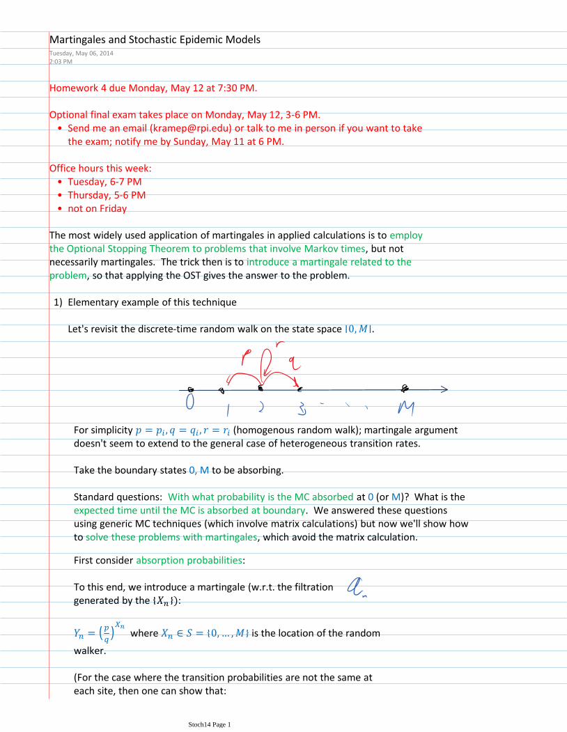
Let's revisit the discrete-time random walk on the state space

For simplicity (homogenous random walk); martingale argument doesn't seem to extend to the general case of heterogeneous transition rates.

Take the boundary states 0, M to be absorbing.

Standard questions: With what probability is the MC absorbed at 0 (or M)? What is the expected time until the MC is absorbed at boundary. We answered these questions using generic MC techniques (which involve matrix calculations) but now we'll show how to solve these problems with martingales, which avoid the matrix calculation.

First consider absorption probabilities:

To this end, we introduce a martingale (w.r.t. the filtration generated by the :

where is the location of the random

walker.

(For the case where the transition probabilities are not the same at each site, then one can show that:

Martingales and Stochastic Epidemic ModelsTuesday, May 06, 20142:03 PM

Stoch14 Page 1

is the appropriate martingale.

Let's first check that what we've constructed is a martingale; it is actually just an example of a general family of exponential martingales.

Nope, doesn't seem to work.

Stoch14 Page 2

What about the technical condition:

is a simple consequence of having a finite state space.

Let's now combine this martingale with the Markov time .

Let's see if we can apply the Optional Stopping Theorem. Three conditions to check. First two are easy; third one is not difficult to verify.

Then the conclusion is: .

Now unwind it, assuming that

Stoch14 Page 3

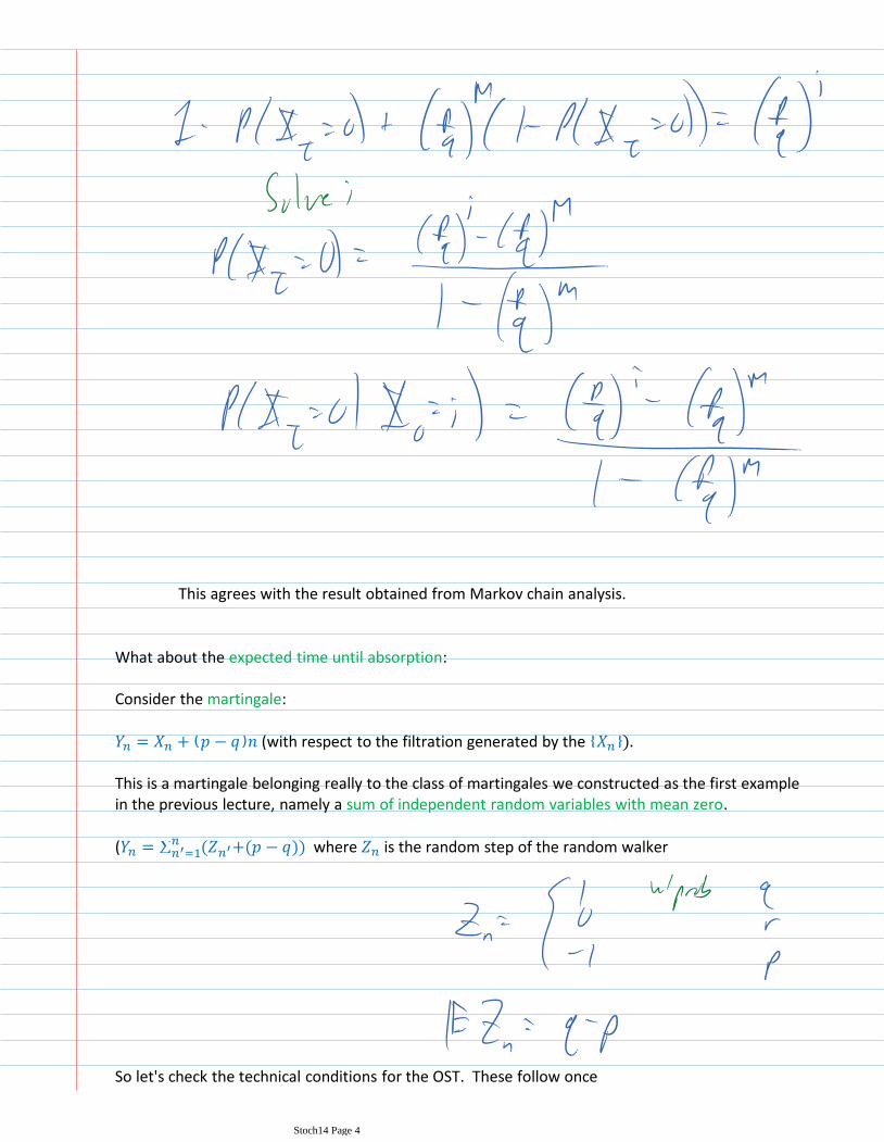
This agrees with the result obtained from Markov chain analysis.

What about the expected time until absorption:

Consider the martingale:

(with respect to the filtration generated by the

This is a martingale belonging really to the class of martingales we constructed as the first example in the previous lecture, namely a sum of independent random variables with mean zero.

( where is the random step of the random walker

So let's check the technical conditions for the OST. These follow once one establishes that the probability distribution for the Markov time

Stoch14 Page 4

one establishes that the probability distribution for the Markov time falls off at least geometrically (use the argument involving the finite number of transient states).

If we take initial condition and condition on it:

Other more sophisticated examples of applying martingales to compute answers to Markov time problems:

Stoch14 Page 5

○ Karlin and Taylor Sec. 6.4: pricing American options

○ Karlin and Taylor Sec. 6.6c: probability distribution for the time between branching events in a continuous-time version of a branching process

problems:

Stochastic Epidemic Models

Andersson and Britton, Stochastic Epidemic Models and Their Statistical Analysis, Ch. 2.

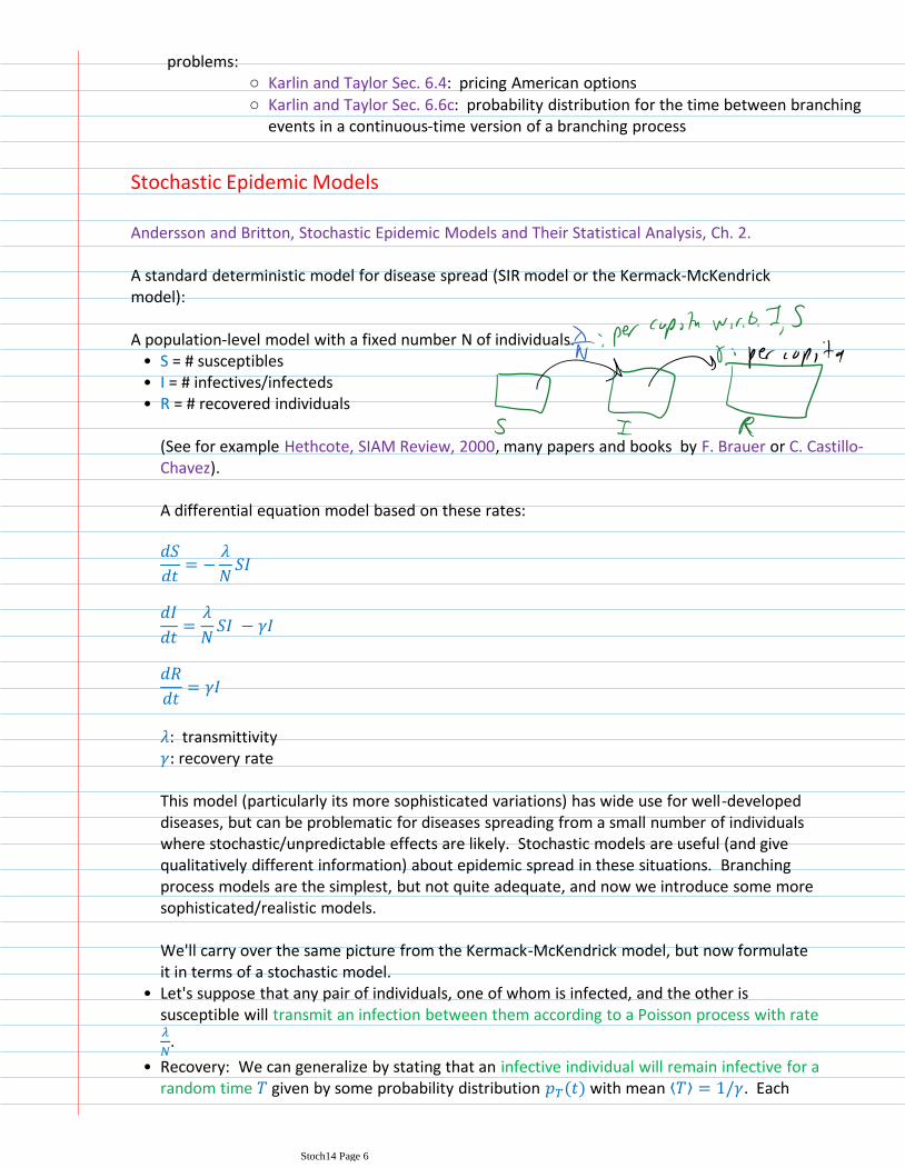
A standard deterministic model for disease spread (SIR model or the Kermack-McKendrick model):

• S = # susceptibles• I = # infectives/infecteds• R = # recovered individuals

(See for example Hethcote, SIAM Review, 2000, many papers and books by F. Brauer or C. Castillo-Chavez).

A differential equation model based on these rates:

: transmittivity recovery rate

This model (particularly its more sophisticated variations) has wide use for well-developed diseases, but can be problematic for diseases spreading from a small number of individuals where stochastic/unpredictable effects are likely. Stochastic models are useful (and give qualitatively different information) about epidemic spread in these situations. Branching process models are the simplest, but not quite adequate, and now we introduce some more sophisticated/realistic models.

We'll carry over the same picture from the Kermack-McKendrick model, but now formulate it in terms of a stochastic model.

• Let's suppose that any pair of individuals, one of whom is infected, and the other is susceptible will transmit an infection between them according to a Poisson process with rate

.

• Recovery: We can generalize by stating that an infective individual will remain infective for a random time given by some probability distribution with mean . Each infective period of an individual is independent of the infective periods of other individuals.

A population-level model with a fixed number N of individuals.

Stoch14 Page 6

infective period of an individual is independent of the infective periods of other individuals.

• If

( (deterministic)): Then one can formulate a discrete-time

Markov chain with epochs being given by periods of length

so that each infective period is

one epoch. This is essentially the Reed-Frost model (Section 1.2 of Andersson and Britton).• If is exponentially distributed, then the stochastic SIR can be formulated as a

continuous-time Markov chain with the following reactions:

Special cases of this stochastic SIR model:

But neither of these models for recovery is particularly realistic, and then the model does not fall into the category of a Markov process for the same reason that a renewal process is not a Markov process. But still, there is some loss of memory in the system; the memory is simply the clocks for infection of the currently infective people. Simulating this is not difficult.

But how do we analyze the model other than by simulation? A key tool is the Sellke construction.

• Sellke construction• optional stopping theorem for martingales

Suppose we start with a population of m infective people and n susceptible people, for a total of N=n+m individuals. Can we develop a deterministic scheme for computing the probability distribution for the total number of individuals that become infected? Yes, this is done in Andersson and Britton Ch. 2. Essential ideas:

Sellke construction is an equivalent alternative for the general stochastic SIR model:

Define infection pressure :

where is the number of infective individuals at time t. (S(t) is the number of susceptible individuals at time t.)

Associate to each susceptible individual an infection threshold which are iid random

variables with Exp(1).

Individual j becomes infective at the time t (if it ever happens) when

Stoch14 Page 7

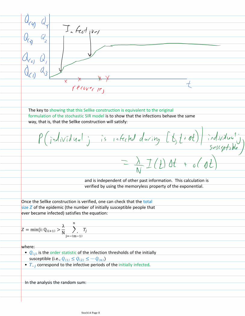
The key to showing that this Sellke construction is equivalent to the original formulation of the stochastic SIR model is to show that the infections behave the same way, that is, that the Sellke construction will satisfy:

and is independent of other past information. This calculation is verified by using the memoryless property of the exponential.

Once the Sellke construction is verified, one can check that the total size of the epidemic (the number of initially susceptible people that ever became infected) satisfies the equation:

• is the order statistic of the infection thresholds of the initially

susceptible (i.e.,

• correspond to the infective periods of the initially infected.

where:

In the analysis the random sum:

Stoch14 Page 8

plays a key role. It is the total infection pressure from the epidemic (actually subepidemics). This looks like the kind of random sum we handled with generating functions, but we can't do it here because the number of terms in the sum is not independent of the terms in the sum.

That means in particular that one cannot compute:

So the resolution to do the calculations is to apply the optional stopping theorem to the random sum in the form of what's called a Wald identity. The random variable plays the role of a Markov time.

The probability distribution for the final size typically has a bimodal character.

Stoch14 Page 9