Mars Atmosphere and Volatile Evolution

(MAVEN) Mission

Langmuir Probe and Waves Instrument (excluding EUV)

PDS Archive

Software Interface Specification

[Rev. 2.0 May 15, 2015]

Prepared by

Laila Andersson

laila.andersson@lasp.colorado.edu

MAVEN

Langmuir Probe and Waves Instrument (excluding EUV)

PDS Archive

Software Interface Specification

[Rev. 2.0 May 15, 2015]

Custodian:

Laila Andersson Date

LPW Archivist

Approved:

Robert R Ergun Date

LPW Principal Investigator

Frank Eparvier Date

EUV Lead/Archivist

David L. Mitchell Date

MAVEN SDWG Lead

Alexandria DeWolfe Date

MAVEN Science Data Center

Raymond J. Walker Date

PDS PPI Node Manager

Thomas H. Morgan Date

PDS Project Manager

Contents

1 Introduction ................................................................................................................................... 1

1.1 Distribution List ....................................................................................................................1

1.2 Document Change Log ..........................................................................................................1

1.3 TBD Items .............................................................................................................................1

1.4 Abbreviations ........................................................................................................................2

1.5 Glossary .................................................................................................................................4

1.6 MAVEN Mission Overview ..................................................................................................7

1.6.1 Mission Objectives ..........................................................................................................7

1.6.2 Payload ............................................................................................................................8

1.7 SIS Content Overview ...........................................................................................................8

1.8 Scope of this document .........................................................................................................9

1.9 Applicable Documents ..........................................................................................................9

1.10 Audience ..............................................................................................................................9

2 LPW Instrument Description .................................................................................................... 10

2.1 Science Objectives ..............................................................................................................10

2.2 Measurement techniques .....................................................................................................11

2.3 Detectors and Electronics ....................................................................................................13

2.4 Operational Modes ..............................................................................................................14

2.5 Measured Parameters ..........................................................................................................15

2.6 Operational Considerations .................................................................................................16

2.7 Ground Calibration ..............................................................................................................17

2.8 Inflight Calibration ..............................................................................................................17

2.9 References ...........................................................................................................................18

3 Data Overview ............................................................................................................................. 19

3.1 Data Processing Levels .......................................................................................................19

3.2 Products ...............................................................................................................................20

3.3 Product Organization ...........................................................................................................20

3.3.1 Collection and Basic Product Types .............................................................................21

3.4 Bundle Products ..................................................................................................................22

3.5 Data Flow ............................................................................................................................23

4 Archive Generation ..................................................................................................................... 25

4.1 Data Processing and Production Pipeline ............................................................................25

4.1.1 Raw Data Production Pipeline ......................................................................................25

4.1.2 Calibrated Data Production Pipeline .............................................................................25

4.2 Data Validation ....................................................................................................................26

4.2.1 Instrument Team Validation ..........................................................................................26

4.2.2 MAVEN Science Team Validation ...............................................................................26

4.2.3 PDS Peer Review ..........................................................................................................26

4.3 Data Transfer Methods and Delivery Schedule ..................................................................27

4.4 Data Product and Archive Volume Size Estimates .............................................................29

4.5 Data Validation ....................................................................................................................29

4.6 Backups and duplicates .......................................................................................................29

5 Archive organization and naming ............................................................................................. 31

5.1 Logical Identifiers ...............................................................................................................31

5.1.1 LID Formation ...............................................................................................................31

5.1.2 VID Formation ..............................................................................................................32

5.2 LPW Archive Contents .......................................................................................................32

5.2.1 LPW raw ........................................................................................................................32

5.2.2 LPW calibrated ..............................................................................................................36

5.2.3 LPW derived ..................................................................................................................49

5.2.4 LPW documentation ......................................................................................................53

6 Archive product formats ............................................................................................................ 55

6.1 Data File Formats ................................................................................................................55

6.1.1 Raw file data structure ...................................................................................................58

6.1.2 Calibrated data file structure .........................................................................................59

6.1.3 Derived data file structure .............................................................................................60

6.2 Document Product File Formats ..........................................................................................62

6.3 PDS Labels ..........................................................................................................................62

6.3.1 XML Documents ...........................................................................................................62

6.4 Delivery Package .................................................................................................................63

6.4.1 The Package ..................................................................................................................63

6.4.2 Transfer Manifest ..........................................................................................................63

6.4.3 Checksum Manifest .......................................................................................................63

Appendix A Support staff and cognizant persons ..................................................................... 64

Appendix B Naming conventions for MAVEN science data files ........................................... 65

Appendix C Sample Bundle Product Label ............................................................................... 66

Appendix D Sample Collection Product Label .......................................................................... 67

Appendix E Sample Data Product Labels ................................................................................. 68

Appendix F PDS Delivery Package Manifest File Record Structures.................................... 69

F.1 Transfer Package Directory Structure .................................................................................69

F.2 Transfer Manifest Record Structure ....................................................................................69

F.3 Checksum Manifest Record Structure ................................................................................69

List of Figures

Figure 1: The location of the LPW sensors on MAVEN. ............................................................. 10

Figure 2: Block diagram of LPW instrument (including EUV) ................................................... 11

Figure 3: LPW mechanical design of the sensor and preamp. ...................................................... 13

Figure 4: The planned LPW operation cycle. The LPW cycles through LP and W subcycles to

measure ne, Te, and plasma waves. ....................................................................................... 14

Figure 5: The LPW basic configuration is to operate with a 4 s master cycle at the lowest

altitudes (< ~500 km), a 8-16 s master cycle at mid-altitudes (~500 km to ~2000 km), and a

64-128 s master cycle at high altitudes. ................................................................................ 15

Figure 6: TBR Amplitude response as function of frequency for the different frequency filters.

HF can be operated with a high gain setting (HG). .............................................................. 17

Figure 7: A graphical depiction of the relationship among bundles, collections, and basic

products. ................................................................................................................................ 21

Figure 8: MAVEN Ground Data System responsibilities and data flow. Note that this figure

includes portions of the MAVEN GDS which are not directly connected with archiving, and

are therefore not described in Section 3.5 above. ................................................................. 24

Figure 9: Duplication and dissemination of LPW archive products at PDS/PPI. ......................... 30

List of Tables

Table 1: Distribution list ................................................................................................................. 1

Table 2: Document change log ....................................................................................................... 1

Table 3: List of TBD items ............................................................................................................. 2

Table 4: Abbreviations and their meaning ...................................................................................... 2

Table 5: The low-pass poles of the analog filters. All filters are designed to have linear phase

delay (Bessel) so that the signal shape is preserved. The EMF and EHF signals have a 1-pole

high pass filter at 100 Hz. ..................................................................................................... 14

Table 6: Characteristics of the ELF, EMF and ELF spectra. ............................................................. 16

Table 7: MAVEN LPW Archive Schema and Schematron .......................................................... 19

Table 8: Data processing level designations ................................................................................. 19

Table 9: Collection product types ................................................................................................. 21

Table 10: LPW Bundles ................................................................................................................ 22

Table 11: MAVEN PDS review schedule .................................................................................... 26

Table 12: Archive bundle delivery schedule for LPW ................................................................. 27

Table 13: LPW raw Collection LID.............................................................................................. 32

Table 14: LPW calibrated Main Collection LID .......................................................................... 36

Table 15: LPW calibrated:data sub-Product LID ......................................................................... 36

Table 16: LPW derived Main Collection LID .............................................................................. 49

Table 17: LPW derived Collections .............................................................................................. 49

Table 18: Documentation Collection LID .................................................................................... 53

Table 19: Key Documentation associated with LPW ................................................................... 53

Table 20: CDF specific information in the CDF header in each CDF file. See individual products

for further information (Table 22 to Table 29) .................................................................... 55

Table 21: LPW Header information that exists in each CDF file but might not always be used.

See the individual products which fields are used (Table 22 to Table 29) ........................... 57

Table 22: Contents for lpw.raw data files. .................................................................................... 58

Table 23: Contents for lpw.calibrated:data.mgr.sc_pot data file. ................................................. 59

Table 24: Contents for lpw.calibrated:data.w.e12, lpw.calibrated:data.w.e12burstlf,

lpw.calibrated:data.w.e12burstmf, and lpw.calibrated:data.w.e12bursthf data files. ........... 59

Table 25: Contents for lpw.calibrated:data.w.specact and lpw.calibrated:data.w.specpas data

files. ....................................................................................................................................... 59

Table 26: Contents for lpw.calibrated:data.lp.iv data file. ............................................................ 60

Table 27: Contents for lpw.derived:data.w.n data files. ............................................................... 60

Table 28: Contents for lpw.derived:data.lp.nt data files. .............................................................. 61

Table 29: Contents for lpw.derived:data.mgr.exb data file. ......................................................... 61

Table 30: Archive support staff .................................................................................................... 64

1 Introduction

This software interface specification (SIS) describes the format and content of the Langmuir

Probe and Waves Instrument (excluding EUV) (LPW) Planetary Data System (PDS) data

archive. It includes descriptions of the data products and associated metadata, and the archive

format, content, and generation pipeline.

1.1 Distribution List

Table 1: Distribution list

Name Organization Email

Laila Andersson LASP/LPW Laila.Andersson@lasp.colorado.edu

Bob Ergun LASP/LPW Bob.Ergun@lasp.colorado.edu

Frank Eparvier LASP/EUV Frank.Eparvier@lasp.colorado.edu

David Mitchell SSL/PF mitchell@ssl.berkeley.edu

Alexandria DeWolfe LASP/SDC alex.dewolfe@lasp.colorado.edu

Thomas H. Morgan Goddard/PDS thomas.h.morgan@nasa.gov

Steve Joy UCLA/PDS/PPI sjoy@igpp.ucla.edu

Ray Walker UCLA/PDS/PPI rwalker@igpp.ucla.edu

Joe Mafi UCLA/PDS/PPI jmafi@igpp.ucla.edu

Reta Beebe NMSU/PDS/Atmospheres rbeebe@nmsu.edu

Lyle Huber NMSU/PDS/Atmospheres lhuber@nmsu.edu

Lynn Neakrase NMSU/PDS/Atmospheres lneakras@nmsu.edu

1.2 Document Change Log

Table 2: Document change log

Version Change Date Affected portion

0.0 Initial template 2012-Aug-24 All

0.1 Updated template 2013-Feb-13 All

0.2 Updated template 2013-Apr-03 All

0.3 Updated template 2014-Jan-30 All

0.4 First draft 2014-Mar-1 All

0.5 Second draft 2014-June-4 All

1.0 First Version of the Document 2014-June-18 All

1.3 TBD Items

Table 3 lists items that are not yet finalized.

Table 3: List of TBD items

Item Section(s) Page(s)

Full references for PDS4 Standards

Reference, and Data Provider’s Handbook

documents (to be provided by PDS/PPI)

1.9

Sample labels (to be provided by PDS/PPI) Appendices C, D, and E

1.4 Abbreviations

Table 4: Abbreviations and their meaning

Abbreviation Meaning

ASCII American Standard Code for Information Interchange

Atmos PDS Atmospheres Node (NMSU, Las Cruces, NM)

CCSDS Consultative Committee for Space Data Systems

CDR Calibrated Data Record

CFDP CCSDS File Delivery Protocol

CK C-matrix Kernel (NAIF orientation data)

CODMAC Committee on Data Management, Archiving, and Computing

CRC Cyclic Redundancy Check

CU University of Colorado (Boulder, CO)

DAP Data Analysis Product

DDR Derived Data Record

DMAS Data Management and Storage

DPF Data Processing Facility

E&PO Education and Public Outreach

EDR Experiment Data Record

EUV Extreme Ultraviolet; also used for the EUV Monitor, part of LPW (SSL)

FEI File Exchange Interface

FOV Field of View

FTP File Transfer Protocol

GB Gigabyte(s)

GSFC Goddard Space Flight Center (Greenbelt, MD)

HK Housekeeping

HTML Hypertext Markup Language

Abbreviation Meaning

ICD Interface Control Document

IM Information Model

ISO International Standards Organization

ITF Instrument Team Facility

IUVS Imaging Ultraviolet Spectrograph (LASP)

JPL Jet Propulsion Laboratory (Pasadena, CA)

LASP Laboratory for Atmosphere and Space Physics (CU)

LID Logical Identifier

LIDVID Versioned Logical Identifer

LPW Langmuir Probe and Waves instrument (SSL)

MAG Magnetometer instrument (GSFC)

MAVEN Mars Atmosphere and Volatile EvolutioN

MB Megabyte(s)

MD5 Message-Digest Algorithm 5

MOI Mars Orbit Insertion

MOS Mission Operations System

MSA Mission Support Area

NAIF Navigation and Ancillary Information Facility (JPL)

NASA National Aeronautics and Space Administration

NGIMS Neutral Gas and Ion Mass Spectrometer (GSFC)

NMSU New Mexico State University (Las Cruces, NM)

NSSDC National Space Science Data Center (GSFC)

PCK Planetary Constants Kernel (NAIF)

PDS Planetary Data System

PDS4 Planetary Data System Version 4

PF Particles and Fields (instruments)

PPI PDS Planetary Plasma Interactions Node (UCLA)

RS Remote Sensing (instruments)

SCET Spacecraft Event Time

SDC Science Data Center (LASP)

Abbreviation Meaning

SCLK Spacecraft Clock

SEP Solar Energetic Particle instrument (SSL)

SIS Software Interface Specification

SOC Science Operations Center (LASP)

SPE Solar Particle Event

SPICE Spacecraft, Planet, Instrument, C-matrix, and Events (NAIF data format)

SPK Spacecraft and Planetary ephemeris Kernel (NAIF)

SSL Space Sciences Laboratory (UCB)

STATIC Supra-Thermal And Thermal Ion Composition instrument (SSL)

SWEA Solar Wind Electron Analyzer (SSL)

SWIA Solar Wind Ion Analyzer (SSL)

TBC To Be Confirmed

TBD To Be Determined

UCB University of California, Berkeley

UCLA University of California, Los Angeles

URN Uniform Resource Name

UV Ultraviolet

XML eXtensible Markup Language

1.5 Glossary

Archive – A place in which public records or historical documents are preserved; also the

material preserved – often used in plural. The term may be capitalized when referring to all of

PDS holdings – the PDS Archive.

Basic Product – The simplest product in PDS4; one or more data objects (and their description

objects), which constitute (typically) a single observation, document, etc. The only PDS4

products that are not basic products are collection and bundle products.

Bundle Product – A list of related collections. For example, a bundle could list a collection of

raw data obtained by an instrument during its mission lifetime, a collection of the calibration

products associated with the instrument, and a collection of all documentation relevant to the

first two collections.

Class – The set of attributes (including a name and identifier) which describes an item defined in

the PDS Information Model. A class is generic – a template from which individual items may be

constructed.

Collection Product – A list of closely related basic products of a single type (e.g. observational

data, browse, documents, etc.). A collection is itself a product (because it is simply a list, with its

label), but it is not a basic product.

Data Object – A generic term for an object that is described by a description object. Data

objects include both digital and non-digital objects.

Description Object – An object that describes another object. As appropriate, it will have

structural and descriptive components. In PDS4 a ‘description object’ is a digital object – a string

of bits with a predefined structure.

Digital Object – An object which consists of real electronically stored (digital) data.

Identifier – A unique character string by which a product, object, or other entity may be

identified and located. Identifiers can be global, in which case they are unique across all of PDS

(and its federation partners). A local identifier must be unique within a label.

Label – The aggregation of one or more description objects such that the aggregation describes a

single PDS product. In the PDS4 implementation, labels are constructed using XML.

Logical Identifier (LID) – An identifier which identifies the set of all versions of a product.

Versioned Logical Identifier (LIDVID) – The concatenation of a logical identifier with a

version identifier, providing a unique identifier for each version of product.

Manifest - A list of contents.

Metadata – Data about data – for example, a ‘description object’ contains information

(metadata) about an ‘object.’

Non-Digital Object – An object which does not consist of digital data. Non-digital objects

include both physical objects like instruments, spacecraft, and planets, and non-physical objects

like missions, and institutions. Non-digital objects are labeled in PDS in order to define a unique

identifier (LID) by which they may be referenced across the system.

Object – A single instance of a class defined in the PDS Information Model.

PDS Information Model – The set of rules governing the structure and content of PDS

metadata. While the Information Model (IM) has been implemented in XML for PDS4, the

model itself is implementation independent.

Product – One or more tagged objects (digital, non-digital, or both) grouped together and having

a single PDS-unique identifier. In the PDS4 implementation, the descriptions are combined into

a single XML label. Although it may be possible to locate individual objects within PDS (and to

find specific bit strings within digital objects), PDS4 defines ‘products’ to be the smallest

granular unit of addressable data within its complete holdings.

Tagged Object – An entity categorized by the PDS Information Model, and described by a PDS

label.

Registry – A database that provides services for sharing content and metadata.

Repository – A place, room, or container where something is deposited or stored (often for

safety).

XML – eXtensible Markup Language.

XML schema – The definition of an XML document, specifying required and optional XML

elements, their order, and parent-child relationships.

1.6 MAVEN Mission Overview

The MAVEN mission is scheduled to launch on an Atlas V between November 18 and

December 7, 2013. After a ten-month ballistic cruise phase, Mars orbit insertion will occur on or

after September 22, 2014. Following a 5-week transition phase, the spacecraft will orbit Mars at

a 75 inclination, with a 4.5 hour period and periapsis altitude of 140-170 km (density corridor of

0.05-0.15 kg/km3). Over a one-Earth-year period, periapsis will presses over a wide range of

latitude and local time, while MAVEN obtains detailed measurements of the upper atmosphere,

ionosphere, planetary corona, solar wind, interplanetary/Mars magnetic fields, solar EUV and

solar energetic particles, thus defining the interactions between the Sun and Mars. MAVEN will

explore down to the homopause during a series of five 5-day “deep dip” campaigns for which

periapsis will be lowered to an atmospheric density of 2 kg/km3 (~125 km altitude) in order to

sample the transition from the collisional lower atmosphere to the collisionless upper

atmosphere. These five campaigns will be interspersed though the mission to sample the subsolar

region, the dawn and dusk terminators, the anti-solar region, and the North Pole.

1.6.1 Mission Objectives

The primary science objectives of the MAVEN project will be to provide a comprehensive

picture of the present state of the upper atmosphere and ionosphere of Mars and the processes

controlling them and to determine how loss of volatiles to outer space in the present epoch varies

with changing solar conditions. Knowing how these processes respond to the Sun’s energy inputs

will enable scientists, for the first time, to reliably project processes backward in time to study

atmosphere and volatile evolution. MAVEN will deliver definitive answers to high-priority

science questions about atmospheric loss (including water) to space that will greatly enhance our

understanding of the climate history of Mars. Measurements made by MAVEN will allow us to

determine the role that escape to space has played in the evolution of the Mars atmosphere, an

essential component of the quest to “follow the water” on Mars. MAVEN will accomplish this

by achieving science objectives that answer three key science questions:

What is the current state of the upper atmosphere and what processes control it?

What is the escape rate at the present epoch and how does it relate to the controlling

processes?

What has the total loss to space been through time?

MAVEN will achieve these objectives by measuring the structure, composition, and variability

of the Martian upper atmosphere, and it will separate the roles of different loss mechanisms for

both neutrals and ions. MAVEN will sample all relevant regions of the Martian

atmosphere/ionosphere system—from the termination of the well-mixed portion of the

atmosphere (the “homopause”), through the diffusive region and main ionosphere layer, up into

the collisionless exosphere, and through the magnetosphere and into the solar wind and

downstream tail of the planet where loss of neutrals and ionization occurs to space—at all

relevant latitudes and local solar times. To allow a meaningful projection of escape back in time,

measurements of escaping species will be made simultaneously with measurements of the energy

drivers and the controlling magnetic field over a range of solar conditions. Together with

measurements of the isotope ratios of major species, which constrain the net loss to space over

time, this approach will allow thorough identification of the role that atmospheric escape plays

today and to extrapolate to earlier epochs.

1.6.2 Payload

MAVEN will use the following science instruments to measure the Martian upper atmospheric

and ionospheric properties, the magnetic field environment, the solar wind, and solar radiation

and particle inputs:

NGIMS Package:

o Neutral Gas and Ion Mass Spectrometer (NGIMS) measures the composition,

isotope ratios, and scale heights of thermal ions and neutrals.

RS Package:

o Imaging Ultraviolet Spectrograph (IUVS) remotely measures UV spectra in four

modes: limb scans, planetary mapping, coronal mapping and stellar occultations.

These measurements provide the global composition, isotope ratios, and structure

of the upper atmosphere, ionosphere, and corona.

PF Package:

o Supra-Thermal and Thermal Ion Composition (STATIC) instrument measures the

velocity distributions and mass composition of thermal and suprathermal ions

from below escape energy to pickup ion energies.

o Solar Energetic Particle (SEP) instrument measures the energy spectrum and

angular distribution of solar energetic electrons (30 keV – 1 MeV) and ions (30

keV – 12 MeV).

o Solar Wind Ion Analyzer (SWIA) measures solar wind and magnetosheath ion

density, temperature, and bulk flow velocity. These measurements are used to

determine the charge exchange rate and the solar wind dynamic pressure.

o Solar Wind Electron Analyzer (SWEA) measures energy and angular

distributions of 5 eV to 5 keV solar wind, magnetosheath, and auroral electrons,

as well as ionospheric photoelectrons. These measurements are used to constrain

the plasma environment, magnetic field topology and electron impact ionization

rate.

o Langmuir Probe and Waves (LPW) instrument measures the electron density and

temperature and electric field in the Mars environment. The instrument includes

an EUV Monitor that measures the EUV input into Mars atmosphere in three

broadband energy channels.

o Magnetometer (MAG) measures the vector magnetic field in all regions traversed

by MAVEN in its orbit.

1.7 SIS Content Overview

Section 2 describes the LPW instrument. Section 3 gives an overview of data organization and

data flow. Section 4 describes data archive generation, delivery, and validation. Section 5

describes the archive structure and archive production responsibilities. Section 6 describes the

file formats used in the archive, including the data product record structures. Individuals

involved with generating the archive volumes are listed in Appendix A. Appendix B contains a

description of the MAVEN science data file naming conventions. Appendix C, Appendix D, and

Appendix E contain sample PDS product labels. Appendix F describes LPW archive product

PDS deliveries formats and conventions.

1.8 Scope of this document

The specifications in this SIS apply to all LPW products submitted for archive to the Planetary

Data System (PDS), for all phases of the MAVEN mission. This document includes descriptions

of archive products that are produced by both the LPW team and by PDS.

1.9 Applicable Documents

[1] Planetary Data System Data Provider’s Handbook, TBD.

[2] Planetary Data System Standards Reference, Version 1.2.0, March 27, 2014.

[3] Planetary Science Data Dictionary Document, TBD.

[4] Planetary Data System (PDS) PDS4 Information Model Specification, Version 1.1.0.1.

[5] Mars Atmosphere and Volatile Evolution (MAVEN) Science Data Management Plan, Rev.

C, doc. no. MAVEN-SOPS-PLAN-0068.

[6] Archive of MAVEN CDF in PDS4, Version 3, T. King and J. Mafi, March 13, 2014.

1.10 Audience

This document serves both as a SIS and Interface Control Document (ICD). It describes both the

archiving procedure and responsibilities, and data archive conventions and format. It is designed

to be used both by the instrument teams in generating the archive, and by those wishing to

understand the format and content of the LPW PDS data product archive collection. Typically,

these individuals would include scientists, data analysts, and software engineers.

2 LPW Instrument Description

The LPW instrument measures the electron density (ne) and temperature (Te) of Mars ionosphere

and detects waves that can heat ions in resulting in atmospheric loss. The instrument is designs to

measure three different types of quantities using three sensors located on the spacecraft as shown

in Figure 1. First is the Extreme UltraViolet (EUV) sensor monitoring the irradiance of the Sun.

The details of the EUV sensor and higher order data products are described in a separate SIS

document [7]. The other two quantities are using the same sensors to measure the in-situ plasma.

The sensors are two cylindrical sensors mounted on two ~7-meter booms shown as LPW sensor

1&2 in Figure 1. Electronically the LPW sensor 1&2 are either operated as two separate

Langmuir probe (LP) instruments or as one electric field instrument. The Boom Electronics

Board (BEB) and the Digital Fields Board (DFB) controls the three sensors and process the three

sensor information. The LPW is a part of the Particle and Fields (PF) suite and controlled by

Particle and Fields Digital Processing Unit (PFDPU) described in another document [8]. The

BEB and DFB are part of the PFDPU located inside the spacecraft body, Figure 1.

Figure 1: The location of the LPW sensors on MAVEN.

2.1 Science Objectives

The LPW instrument is designed to measure the electron density and temperature in the

ionosphere of Mars and to measure the spectral power density of waves in Mars’ ionosphere,

including waves that can heat the ions resulting in atmospheric loss. The LPW [9] is part of the

Particle and Fields (PF) suit on the MAVEN spacecraft [10]. The LPW instrument utilizes two,

40 cm long by 0.635 cm diameter cylindrical sensors, which can be configured to measure either

plasma currents or plasma waves. The sensors are mounted on two, ~7-meter long stacer booms.

The sensors and nearby surfaces are controlled by a Boom Electronics Board (BEB), which

allows for operation as either a Langmuir Probe or a wave electric field receiver. The Digital

Fields Board (DFB) conditions the analog signals, converts the analog signals to digital,

processes the digital signals including spectral analysis, and packetizes the data for transmission.

The BEB and DFB are located inside of the Particle and Fields Digital Processing Units

(PFDPU) [8]. One part of the instrument, the Extreme UltraViolet sensor [11], is described in a

companion SIS [7]. The EUV signals are received and processed by the LPW so the EUV signal

processing is included to some extent in this document.

Figure 2: Block diagram of LPW instrument (including EUV)

2.2 Measurement techniques

The electron density and temperature are derived from the current-voltage (I-V) characteristic, a

well-established technique. With this technique, the current from the plasma to a voltage-biased

probe is measured over a range of probe voltages, creating an I-V characteristic. I-V

characteristics are fit to determine the ne, Te, ion density (ni), and spacecraft potential (VSC). The

“LP sweep” contains 128 programmable voltages inside of -50 V to 50 V range. The minimum

step size is ~25 mV. The sweeps are performed in one second (configurable) and are pseudo-

logarithmic, designed to have the smallest steps near zero potential. The dwell time at each step

7.8 ms in the nominal configuration for Mars’ ionosphere.

To cover the large range of ne and Te, the LPW sensors detect a wide range of probe current (IP),

from -0.02 mA to 0.2 mA at ~30 nA resolution. Here, positive current is electron collection. The

resolution is limited by the analog-to-digital conversion (16 bit).

This measurement technique, when implemented on a spacecraft, requires several other factors to

be taken into consideration. Two sensors are used for the LP sweep since one or the probes could

be in the spacecraft wake. The ratio of conductive surface area of the sensors to that of the

spacecraft needs to be such that VSC does not significantly change during a sweep. When biased

at a positive voltage, the probe attracts electrons, so the spacecraft must attract an ion current or

emit photoelectrons. Since the ion thermal velocities are considerably lower than that of

electrons, the spacecraft must have a significantly larger collection area compared to the probe

area. On MAVEN, the area ration of the spacecraft to probe surface is ~100. However, the ion

collection by the spacecraft can vary depending on the spacecraft attitude and velocity. The LPW

has an additional feature such that, during an LP sweep, one probe performs the sweep while the

other probe monitors the plasma potential so that a change in VSC can be detected.

VSC is influenced by plasma conditions, spacecraft attitude and velocity, and sunlight so it may

vary dramatically during an orbit. The LP sweep is automatically adjusted to account for VSC.

The “sweep offset” is adjusted to a voltage level at which the absolute value of the current was at

a minimum in the previous sweeps. The instrument can enable an automatic offset adjustment.

The LPW can operate with -45 V < VSC < 45 V.

Photoelectron currents can interfere with the fitting process that determines ne and Te. These

currents come in two forms. The photoelectron fluxes from the spacecraft to the probe are

minimized by a combination of long booms (7 m) and biased surfaces near the sensors (guards

and stubs). The photoelectron currents emitted by the probe to the plasma (or spacecraft) must be

removed in data analysis. Surface treatments of the probe are designed to have small variations

in photoelectron emission.

The absolute accuracy of the ne measurement can be greatly improved (to <5%) if the frequency

of Langmuir waves or upper hybrid waves can be determined. The LPW includes an electric

field wave receiver that covers the frequency range from ~1 Hz to 2 MHz. These data are called

“passive spectra”. The wave power is calculated on board and separated into three different

frequency ranges low (LF), medium (MF) and high (HF). The HF spectra are designed to contain

the plasma line when available (50kHz to 2MHz) and have two gain stages (HF and HF-HG).

The upper hybrid or plasma frequencies within the HF frequency range it correspond to densities

between ~30 cm-3 and 5x104 cm-3. The LF spectrum is designed to monitor the available power

to heat ions close to the ion gyro-frequencies. These spectrums are derived using 1048 points.

The receiver can be sensitive to plasma waves with a spectral power density as low as 3x10-14

(V/m)2/Hz at 1 MHz. The electrostatic cleanliness program on the MAVEN spacecraft did not

include conductive solar arrays, as the process was deemed to expensive, so spacecraft noise may

dominate the noise floor of the plasma wave receiver. The noise floor is to be determined once

MAVEN is in orbit around Mars.

Since naturally occurring plasma waves may not be detected frequently, the MAVEN LPW can

stimulate the surrounding plasma with a 5 V pseudo-random sequence using the stacer booms as

transmitting elements. This relaxation sounding technique measures the plasma frequency in

quiet environments. The sequence is to broadcast simultaneously on both antennas, receive the

plasma wave electric field immediately after the broadcast is turned off, and record the spectra.

These data are called “active spectra”.

The low-frequency electric field measurement includes piecewise continuous waveforms of one

component of the electric field with a range of +1 V/m and a resolution 0.3 mV/m. The data

processing also includes LF spectra (10 Hz – 1 kHz) and MF spectra (100 Hz – 16 kHz).

The instrument can also record the time series of the electric field measurements that is the base

for the onboard spectra in special operation modes. In the High Speed Burst Mode (HSBM)

high-resolution time series are recorded. The number of points used for the three time series are

1048, 4096, and 4096 for LF, MF, and HF, respectively. Only the largest amplitude cases of

HSBM is recorded and sent to the archive memory in PF. The data stored in the archived

memory can be selected from ground to be downloaded later. Due to the data volume, the HSBM

data is infrequently collected.

2.3 Detectors and Electronics

Following text is a brief description of the instrument, a more detail description is provided in

Andersson et al. [9].

The two cylindrical sensors are mounted on two ~7-m long stacers. They are mounted

approximately 90 degrees to each other and on the spacecraft so that most of the time always

one of the booms is outside any spacecraft wake and far away from the solar panels (Figure 1).

The line between the two sensors is along the y-axis of the spacecraft coordinate.

The LPW sensors are diagramed in Figure 3. The sensor or “whip” is a 40 cm by 0.635 cm

titanium tube with a TiN surface Erikson et al. [12], which acts as the physical collection area

(~80 cm2). This area is roughly 100 times smaller than the expected collection area of the

spacecraft. The sensor is electrically connected to the inputs of the preamplifiers. The collection

area results in ~20 nA at the lowest densities (~102 cm-3) and ~0.2 mA if the density were to

reach 106 cm-3. The cylindrical sensor has the advantage that the current collection properties (e.

g., focus factor) are well behaved and well understood (analytically).

The signal-processing unit for the LPW instrument contains two circuit boards, the Boom

Electronics Board (BEB) and the Digital Fields Board (DFB), which are located in the PFDPU.

The LP and W preamplifiers on the 2 booms and the EUV sensors are connected to the BEB or

DFB as illustrated in Figure 2. The LPW commands arrive via the PFDPU and data packets from

the LPW are sent via the PFDPU for transmission (survey data) or stored in the archive location

in the PFDPU to be later selected for down link (archive data).

The LPW, once configured, operates the sweeps and cycles through the measurements

independently. The spacecraft controls the one time boom deployment, the one time EUV door

deployment, and the heaters on the EUV and the boom. The spacecraft provides alerts to the

PFDPU for the LPW. The PFDPU holds configuration tables for the LPW in EEPROM. The

PFDPU also passes operation commands to the LPW and maintains the archive memory. The

PFDPU controls the EUV aperture.

Figure 3: LPW mechanical design of the sensor and preamp.

The DFB receives and conditions the science and engineering signals listed in Table 5: The low-

pass poles of the analog filters. All filters are designed to have linear phase delay (Bessel) so that

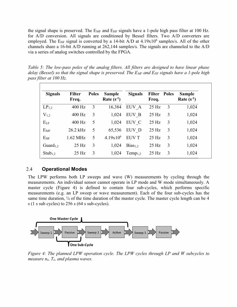
the signal shape is preserved. The EMF and EHF signals have a 1-pole high pass filter at 100 Hz.

for A/D conversion. All signals are conditioned by Bessel filters. Two A/D converters are

employed. The EHF signal is converted by a 14-bit A/D at 4.19x106 samples/s. All of the other

channels share a 16-bit A/D running at 262,144 samples/s. The signals are channeled to the A/D

via a series of analog switches controlled by the FPGA.

Table 5: The low-pass poles of the analog filters. All filters are designed to have linear phase

delay (Bessel) so that the signal shape is preserved. The EMF and EHF signals have a 1-pole high

pass filter at 100 Hz.

Signals Filter

Freq.

Poles Sample

Rate (s-1)

Signals Filter

Freq.

Poles Sample

Rate (s-1)

LP1,2 400 Hz 3 16,384 EUV_A 25 Hz 3 1,024

V1,2 400 Hz 3 1,024 EUV_B 25 Hz 3 1,024

ELF 400 Hz 5 1,024 EUV_C 25 Hz 3 1,024

EMF 26.2 kHz 5 65,536 EUV_D 25 Hz 3 1,024

EHF 1.62 MHz 5 4.19x106 EUV T 25 Hz 3 1,024

Guard1,2 25 Hz 3 1,024 Bias1,2 25 Hz 3 1,024

Stub1,2 25 Hz 3 1,024 Temp1,2 25 Hz 3 1,024

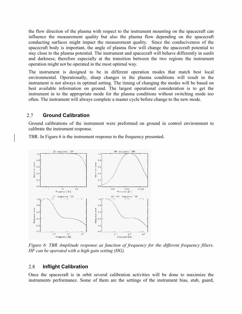
2.4 Operational Modes

The LPW performs both LP sweeps and wave (W) measurements by cycling through the

measurements. An individual sensor cannot operate in LP mode and W mode simultaneously. A

master cycle (Figure 4) is defined to contain four sub-cycles, which performs specific

measurements (e.g. an LP sweep or wave measurement). Each of the four sub-cycles has the

same time duration, ¼ of the time duration of the master cycle. The master cycle length can be 4

s (1 s sub cycles) to 256 s (64 s sub-cycles).

Figure 4: The planned LPW operation cycle. The LPW cycles through LP and W subcycles to

measure ne, Te, and plasma waves.

The planned master cycle is outlined in Figure 4. The LPW instrument begins by performing a

128-point LP sweep on sensor 1, labeled Sweep 1 in Figure 4, while recording the DC potential

on sensor 2. Next, both sensors are set to W mode and wave spectra and time series of the

electric field are taken. The LPW then performs a LP sweep on sensor 2 while recording the DC

potential on sensor 1. The last sub-cycle executes the relaxation sounder. A white-noise

transmission is made on the stacers and the wave spectra are recorded.

Figure 5: The LPW basic configuration is to operate with a 4 s master cycle at the lowest

altitudes (< ~500 km), a 8-16 s master cycle at mid-altitudes (~500 km to ~2000 km), and a 64-

128 s master cycle at high altitudes.

Since the science focus of the LPW instrument is at low-altitudes (< ~500 km) and during deep

dips, the master cycle length at low altitudes is configured to 4 s, the fastest operation (Figure 5).

Between ~500 km and ~2000 km there are several important plasma boundaries. The plasma

density is lower, so the master cycle is set to 8-16 s. For a 16 second master cycle, this allows for

4 s sweeps with ~30 ms dwell times. At higher altitudes, the master cycle is set to 64-128 s,

primarily for solar wind monitoring. Data limitations play an important role in the LPW

operations. Roughly 80% of the data allocation is used below ~500 km.

The LWP sweep tables, sensor biasing, and biasing tables for the guards and stubs are re-

configured to optimize the measurements over a large range of plasma conditions. The sweep

tables, for example, have a narrow voltage range at low altitudes where dense plasma is expected

(-5 V to 5 V; see discussion on automatic offset adjustment). The voltage range is expanded

when in the solar wind to -45 V to 45 V. Adjustments are also made if the spacecraft is in Mars’

umbra. These adjustments are based on the predicted orbit (time-tagged commands).

2.5 Measured Parameters

The LPW measure different products depending on which sub-cycle the instrument is in. There

is some flexibility to modify the products, but presented below is the baseline.

Sweep 1 sub-cycle: The current at each 128 point voltage sweep on Boom 1 are recorded

together with the potential on boom 2, also 128 points. The cadence depends on the master cycle

length.

Sweep 2 sub-cycle: Exactly the same as Sweep 1 but the boom numbers is reversed.

Active sub-cycle: Low frequency potential on boom1 (V1), boom2 (V2), and the electric field

(E12). There are 64 points per sub-cycle and the cadence depends on the master cycle length.

Also the there spectrum LF, MF, and HF is produced.

Passive sub-cycle: Produces the same products as the Active sub-cycle but also can produce the

LF, MF, and HF HSBM time series.

EUV parameters: When LPW is on EUV is sampling data. During normal operation EUV

produce 1 sample per second. EUV sampling cadence is independent on the master cycle period.

House keeping parameters: Infrequent data information for monitoring the instrument health and

operation state. There are three different sets of data; engineering information about the

instrument, the active mode tables sent down and the active settings read back.

Table 6: Characteristics of the ELF, EMF and ELF spectra.

Analog

Filtering

Digital Processing Power Spectral

Density

Signal Gain Low

Pass

-3 dB

(Hz)

High

Pass

-3 dB

(Hz)

Sample

Rate

(s-1)

Freq.

Min.

(Hz)

Freq.

Max.

(Hz)

#

Freq.

Bins

(f/f)

Ave.

(df/f)

Min.

(df/f)

Max.

Receiver

Sensitivity

(V/m)2/Hz

Narrow

Band Range

(V/m)2/Hz

ELF DC 400 1024 0.5 7.5 8 f = 1 Hz 8x10-12 6x10-2

8.5 496 48 9% 6.5% 12% 3x10-12 6x10-2

EMF 100 2.6x104 6.6x104 32 480 8 f = 64 Hz 5x10-15 4x10-5

544 3.2x104 48 9% 6.5% 12% 2x10-15 4x10-5

EHF

Low 100 1.6x106 4.2x106 2048 9.6x104 24 f = 4096 Hz 10-15 2x10-6

1x105 2.1 x106 104 3.1% 2.1% 4.1% 5x10-16 2x10-6

High 100 1.6x106 4.2x106 2048 9.6x104 24 f = 4096 Hz 10-17 10-7

1x105 2.1 x106 104 3.1% 2.1% 4.1% 2x10-17 10-7

2.6 Operational Considerations

There are multiple external effects that will impact the quality of the LPW instrument. The

instrument is designed to be on a sun-pointing platform. Due to different restrictions, the

spacecraft platform will not always be sun-pointing, impacting the data quality. Also, some of

the flow direction of the plasma with respect to the instrument mounting on the spacecraft can

influence the measurement quality but also the plasma flow depending on the spacecraft

conducting surfaces might impact the measurement quality. Since the conduciveness of the

spacecraft body is important, the angle of plasma flow will change the spacecraft potential to

stay close to the plasma potential. The instrument and spacecraft will behave differently in sunlit

and darkness; therefore especially at the transition between the two regions the instrument

operation might not be operated in the most optimal way.

The instrument is designed to be in different operation modes that match best local

environmental. Operationally, sharp changes in the plasma conditions will result in the

instrument is not always in optimal setting. The timing of changing the modes will be based on

best available information on ground. The largest operational consideration is to get the

instrument in to the appropriate mode for the plasma conditions without switching mode too

often. The instrument will always complete a master cycle before change to the new mode.

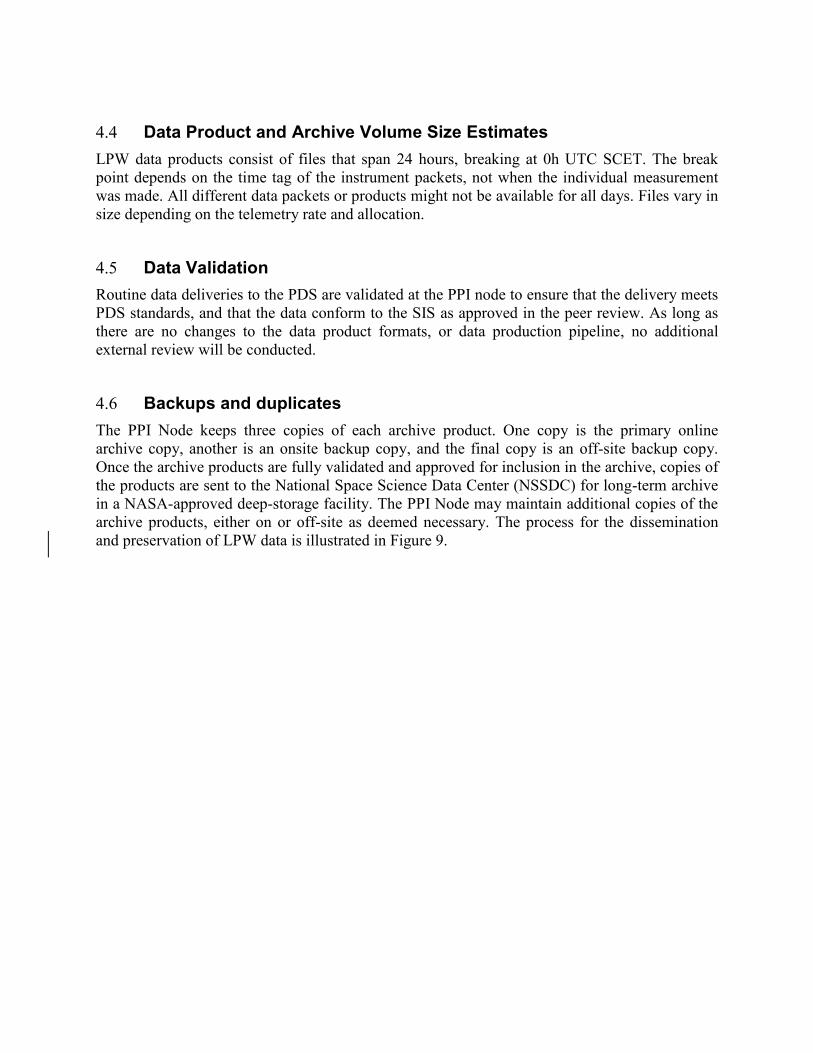
2.7 Ground Calibration

Ground calibrations of the instrument were preformed on ground in control environment to

calibrate the instrument response.

TBR. In Figure 6 is the instrument response to the frequency presented.

Figure 6: TBR Amplitude response as function of frequency for the different frequency filters.

HF can be operated with a high gain setting (HG).

2.8 Inflight Calibration

Once the spacecraft is in orbit several calibration activities will be done to maximize the

instruments performance. Some of them are the settings of the instrument bias, stub, guard,

sweep tables, and master cycle length. All of these calibrations need to be done with respect to

which plasma environment the instrument is in and if the instrument is sunlit or not.

As expected, the instrument in stowed configuration is impacted by thruster firing and reaction

wheel activity. This will be corrected for in the archived L2-data products.

2.9 References

[7] EUV SIS document TBR

[8] Particle and Fields Digital Processing Unit (PFDPU) paper TBR

[9] LPW paper TBR

[10] Particle and Fields suite paper TBR

[11] EUV paper TBR

[12] TiN surface Eriksson et al, 2007 TBR

[13] MAG SIS document TBR

[14] MAG paper TBR

3 Data Overview

This section provides a high level description of archive organization under the PDS4

Information Model (IM) as well as the flow of the data from the spacecraft through delivery to

PDS. Unless specified elsewhere in this document, the MAVEN LPW archive conforms with

version 1.1.0.1 of the PDS4 IM [4] and version 1.0 of the MAVEN mission schema. A list of the

XML Schema and Schematron documents associated with this archive are provided in Table 7

below.

Table 7: MAVEN LPW Archive Schema and Schematron

XML Document Steward Product LID

PDS Master Schema, v.

1.1.0.1 PDS urn:nasa:pds:system_bundle:xml_schema:pds-xml_schema

PDS Master Schematron, v.

1.1.0.1

PDS urn:nasa:pds:system_bundle:xml_schema:pds-xml_schema

MAVEN Mission Schema,

v. 1.0

MAVEN

MAVEN Mission

Schematron, v. 1.0 MAVEN

3.1 Data Processing Levels

A number of different systems may be used to describe data processing level. This document

refers to data by their PDS4 processing level. Table 8 provides a description of these levels along

with the equivalent designations used in other systems.

Table 8: Data processing level designations

PDS4

processing

level

PDS4 processing level description

MAVEN

Processing

Level

CODMAC

Level

NASA

Level

Raw

Original data from an instrument. If compression,

reformatting, packetization, or other translation has

been applied to facilitate data transmission or

storage, those processes are reversed so that the

archived data are in a PDS approved archive

format.

0 2 1A

Reduced

Data that have been processed beyond the raw

stage but which are not yet entirely independent of

the instrument. 1 2 1A

Calibrated Data converted to physical units entirely

independent of the instrument. 2 3 1B

PDS4

processing

level

PDS4 processing level description

MAVEN

Processing

Level

CODMAC

Level

NASA

Level

Derived

Results that have been distilled from one or more

calibrated data products (for example, maps,

gravity or magnetic fields, or ring particle size

distributions). Supplementary data, such as

calibration tables or tables of viewing geometry,

used to interpret observational data should also be

classified as ‘derived’ data if not easily matched to

one of the other three categories.

3+ 4+ 2+

3.2 Products

A PDS product consists of one or more digital and/or non-digital objects, and an accompanying

PDS label file. Labeled digital objects are data products (i.e. electronically stored files). Labeled

non-digital objects are physical and conceptual entities which have been described by a PDS

label. PDS labels provide identification and description information for labeled objects. The PDS

label defines a Logical Identifier (LID) by which any PDS labeled product is referenced

throughout the system. In PDS4 labels are XML formatted ASCII files. More information on the

formatting of PDS labels is provided in Section 6.3. More information on the usage of LIDs and

the formation of MAVEN LIDs is provided in Section 5.1.

3.3 Product Organization

The highest level of organization for PDS archive is the bundle. A bundle is a list of one or more

related collection products which may be of different types. A collection is a list of one or more

related basic products which are all of the same type. Figure 7 below illustrates these

relationships.

Figure 7: A graphical depiction of the relationship among bundles, collections, and basic

products.

Bundles and collections are logical structures, not necessarily tied to any physical directory

structure or organization. Bundle and collection membership is established by a member

inventory list. Bundle member inventory lists are provided in the bundle product labels

themselves. Collection member inventory lists are provided in separate collection inventory table

files. Sample bundle and collection labels are provided in Appendix C and Appendix D,

respectively.

3.3.1 Collection and Basic Product Types

Collections are limited to a single type of basic products. The types of archive collections that

are defined in PDS4 are listed in Table 9.

Table 9: Collection product types

Collection

Type Description

Browse Contains products intended for data characterization, search, and viewing, and not for

Bundle

Collection A

Basic

Product

A1

Basic

Product

A2

Basic

Product

A3

Basic

Product

AN

…

Collection B

Basic

Product

B1

Basic

Product

B2

Basic

Product

B3

Basic

Product

BN

…

Collection C

Basic

Product

C1

Basic

Product

C2

Basic

Product

C3

Basic

Product

CN

…

scientific research or publication.

Calibration Contains data and files necessary for the calibration of basic products.

Context Contains products which provide for the unique identification of objects which form the

context for scientific observations (e.g. spacecraft, observatories, instruments, targets,

etc.).

Document Contains electronic document products which are part of the PDS Archive.

Data Contains scientific data products intended for research and publication.

SPICE Contains NAIF SPICE kernels.

XML_Schema Contains XML schemas and related products which may be used for generating and

validating PDS4 labels.

3.4 Bundle Products

The LPW data archive is organized into 7 bundles; of which LPW will deliver 4 of the PDS via

SDC for archiving. A description of each bundle is provided in Table 10. A more detailed

description of the contents and format of each bundle controlled by the LPW ITF is provided in

Section 5.2.

Table 10: LPW Bundles

Bundle Logical Identifier

PDS4

Reduction

Level

Description

Data

Provider

TBD Raw PF packets – all packets together,

describe in separated document. This are

L0 files SDC

urn:nasa:pds:maven.lpw.raw Raw LPW packets in separate CDF files.

These are regarded as L0b files TBD

maven.lpw.l1a

– not delivered to PDS

Calibrated/

Derived

Preliminary data, CDF files that might

be deliver to SDC but not to PDS. These

are regarded L1a files.

Contains identical files to

urn:nasa:pds:maven.lpw.calibrated/

urn:nasa:pds:maven.lpw.derived

ITF

maven.lpw.l1b

– not delivered to PDS

Calibrated/

Derived

Preliminary data, CDF files that might

be deliver to SDC but not to PDS. These

are regarded L1b files.

Contains identical files to

urn:nasa:pds:maven.lpw.calibrated/

urn:nasa:pds:maven.lpw.derived

ITF

urn:nasa:pds:maven.lpw.calibrated Calibrated

Fully calibrated: spacecraft potential,

electric field waveforms and wave

power. Provided by the LPW team in

CDF files. These are L2 files.

ITF

urn:nasa:pds:maven.lpw.derived Derived

Derived L2 quantities: density,

temperature, Poynting flux. Provided by

the LPW team in CDF files. These are

L2 files.

ITF

urn:nasa:pds:maven.lpw N/A LPW Documentation ITF

3.5 Data Flow

This section describes only those portions of the MAVEN data flow that are directly connected

to archiving. A full description of MAVEN data flow is provided in the MAVEN Science Data

Management Plan [5]. A graphical representation of the full MAVEN data flow is provided in

Figure 8 below.

Reduced (MAVEN level 1) data will be produced by RS and NGIMS as an intermediate

processing product, and are delivered to the SDC for archiving at the PDS, but will not be used

by the MAVEN team.

All ITFs will produce calibrated products. Following an initial 2-month period at the beginning

of the mapping phase, the ITFs will routinely deliver preliminary calibrated data products to the

SDC for use by the entire MAVEN team within two weeks of ITF receipt of all data needed to

generate those products. The SOC will maintain an active archive of all MAVEN science data,

and will provide the MAVEN science team with direct access through the life of the MAVEN

mission. After the end of the MAVEN project, PDS will be the sole long-term archive for all

public MAVEN data.

Updates to calibrations, algorithms, and/or processing software are expected to occur regularly,

resulting in appropriate production system updates followed by reprocessing of science data

products by ITFs for delivery to SDC. Systems at the SOC, ITFs and PDS are designed to handle

these periodic version changes.

Data bundles intended for the archive are identified in Table 10.

Figure 8: MAVEN Ground Data System responsibilities and data flow. Note that this figure

includes portions of the MAVEN GDS which are not directly connected with archiving, and are

therefore not described in Section 3.5 above.

4 Archive Generation

The LPW archive products are produced by the LPW instrument team in cooperation with the

SDC, and with the support of the PDS, Planetary Plasma Interactions (PPI) Node at the

University of California, Los Angeles (UCLA). The archive volume creation process described

in this section sets out the roles and responsibilities of each of these groups. The assignment of

tasks have been agreed upon by all parties. Archived data received by the PPI Node from the

LPW team are made available to PDS users electronically as soon as practicable but no later two

weeks after the delivery and validation of the data.

4.1 Data Processing and Production Pipeline

The following sections describe the process by which data products in each of the LPW bundles

listed in Table 10 are produced.

4.1.1 Raw Data Production Pipeline

The LPW team use a dedicated decomutator to extract the LPW packets from the raw PF-L0 file

called Pf-L0-file by the MAVEN team. The data from the individual instrument packets is then

extracted and saved as separate CDF files for PDS archiving urn:nasa:pds:maven.lpw.raw,

internally called ‘L0b’-files to separate from the ‘L0’ files. The decomutator software will be

archived at PDS as a reference manual for the future in the Document bundle.

4.1.2 Calibrated Data Production Pipeline

The LPW team use a dedicated decomutator to extract the LPW packets from the raw PF-L0 file

called Pf-L0-file by the MAVEN team. The raw LPW data is then calibrated with the calibration

information derived from ground testing in the instrument constants routine provided in the

Document bundle.

After the individual packets are calibrated using the ground testing data from different packets it

is merged together with ancillary data and evaluated to created the calibrated science products -

L2 (urn:nasa:pds:maven.lpw.calibrated and urn:nasa:pds:maven.lpw.derived). This software is

archived as documentation of the process in the Document bundle.

For processing purposes, the achievable products will be created as L1a and L1b files while

waiting on al ancillary data to become available (the content of these files are identical to the L2

files). The L1a is automatically produced as soon as L0-files are available but before all ancillary

data are available. The L1b is the next step for the products that need manually interaction. The

software to produce L1a, L1b and L2 is the same.

One example of manual interaction is to identify the plasma conditions for fitting of the I-V

sweep. During the production of the L1b files, the sweeps will be analyzed to identify if the I-V

sweep analysis should be assuming a single plasma distribution or multiple. The selected option

will be stored in a separate file and when the automatic L2 production is executed, that process

reads the stored file. This makes any reproduction of the archived data set to be fully automatic

since reprocessing the L2 files will not need any manual interaction.

4.2 Data Validation

4.2.1 Instrument Team Validation

Since the quality of the LPW is sensitive to SC attitude and plasma conditions etc the data will

be evaluated by a scientist through overview plots and spot-checking. At interesting/active

periods the production of the data can be manually optimized. The LPW use confidence flags to

indicate when the SC attitude (or other reasons) degrades the instrument measure quality.

4.2.2 MAVEN Science Team Validation

The calibrated/derived/modeled files will be used by the MAVEN Science team. This will

provide a second validation of the science data. Many of the particle instruments will use the

plasma density derived from the wave measurements for their absolute inflight calibration.

4.2.3 PDS Peer Review

The PPI node will conduct a full peer review of all of the data types that the LPW team intends

to archive. The review data will consist of fully formed bundles populated with candidate final

versions of the data and other products and the associated metadata.

Table 11: MAVEN PDS review schedule

Date Activity Responsible

Team

2014-Mar-24 Signed SIS deadline ITF

2014-Apr-18 Sample data products due ITF

2014-May

to

2014-Aug

Preliminary PDS peer review (SIS, sample data files) PDS

2015-Mar-02 Release #1: Data due to PDS ITF/SDC

2015-Mar

to

2015-Apr

Release #1: Data PDS peer review PDS

2015-May-01 Release #1: Public release PDS

Reviews will include a preliminary delivery of sample products for validation and comment by

PDS PPI and Engineering node personnel. The data provider will then address the comments

coming out of the preliminary review, and generate a full archive delivery to be used for the peer

review.

Reviewers will include MAVEN Project and LPW team representatives, researchers from

outside of the MAVEN project, and PDS personnel from the Engineering and PPI nodes.

Reviewers will examine the sample data products to determine whether the data meet the stated

science objectives of the instrument and the needs of the scientific community and to verify that

the accompanying metadata are accurate and complete. The peer review committee will identify

any liens on the data that must be resolved before the data can be ‘certified’ by PDS, a process

by which data are made public as minor errors are corrected.

In addition to verifying the validity of the review data, this review will be used to verify that the

data production pipeline by which the archive products are generated is robust. Additional

deliveries made using this same pipeline will be validated at the PPI node, but will not require

additional external review.

As expertise with the instrument and data develops the LPW team may decide that changes to the

structure or content of its archive products are warranted. Any changes to the archive products or

to the data production pipeline will require an additional round of review to verify that the

revised products still meet the original scientific and archival requirements or whether those

criteria have been appropriately modified. Whether subsequent reviews require external

reviewers will be decided on a case-by-case basis and will depend upon the nature of the

changes. A comprehensive record of modifications to the archive structure and content is kept in

the Modification_History element of the collection and bundle products.

The instrument team and other researchers are encouraged to archive additional LPW products

that cover specific observations or data-taking activities. The schedule and structure of any

additional archives are not covered by this document and should be worked out with the PPI

node.

4.3 Data Transfer Methods and Delivery Schedule

The SOC is responsible for delivering data products to the PDS for long-term archiving. While

ITFs are primarily responsible for the design and generation of calibrated and derived data

archives, the archival process is managed by the SOC. The SOC (in coordination with the ITFs)

will also be primarily responsible for the design and generation of the raw data archive. The first

PDS delivery will take place within 6 months of the start of science operations. Additional

deliveries will occur every following 3 months and one final delivery will be made after the end

of the mission. Science data are delivered to the PDS within 6 months of its collection. If it

becomes necessary to reprocess data which have already been delivered to the archive, the ITFs

will reprocess the data and deliver them to the SDC for inclusion in the next archive delivery. A

summary of this schedule is provided in Table 12 below.

Table 12: Archive bundle delivery schedule for LPW

Bundle Logical Identifier First Delivery to PDS Delivery Estimated

Delivery

Schedule Size

urn:nasa:pds:maven.lpw.raw Represent L0 data (LPW

team call this is L0b). No

later than 6 months after

the start of science

operations

Every 3 months TBD

urn:nasa:pds:maven.lpw.calibrated Represent L2 data. No

later than 6 months after

the start of science

operations

Every 3 months TBD

urn:nasa:pds:maven.lpw.derived Represent L2 data. No

later than 6 months after

the start of science

operations

Every 3 months TBD

urn:nasa:pds:maven.lpw This SIS document and

the analysis/production

documented software

TBD TBD

Each delivery will comprise both data and ancillary data files organized into directory structures

consistent with the archive design described in Section 5, and combined into a deliverable file(s)

using file archive and compression software. When these files are unpacked at the PPI Node in

the appropriate location, the constituent files will be organized into the archive structure.

Archive deliveries are made in the form of a “delivery package”. Delivery packages include all

of the data being transferred along with a transfer manifest, which helps to identify all of the

products included in the delivery, and a checksum manifest which helps to insure that integrity of

the data is maintained through the delivery. The format of these files is described in Section 6.4.

Data are transferred electronically (using the ssh protocol) from the SOC to an agreed upon

location within the PPI file system. PPI will provide the SOC a user account for this purpose.

Each delivery package is made in the form of a compressed tar or zip archive. Only those files

that have changed since the last delivery are included. The PPI operator will decompress the

data, and verify that the archive is complete using the transfer and MD5 checksum manifests that

were included in the delivery package. Archive delivery status will be tracked using a system

defined by the PPI node.

Following receipt of a data delivery, PPI will reorganize the data into its PDS archive structure

within its online data system. PPI will also update any of the required files associated with a PDS

archive as necessitated by the data reorganization. Newly delivered data are made available

publicly through the PPI online system once accompanying labels and other documentation have

been validated. It is anticipated that this validation process will require no more than fourteen

working days from receipt of the data by PPI. However, the first few data deliveries may require

more time for the PPI Node to process before the data are made publicly available.

The MAVEN prime mission begins approximately 5 weeks following MOI and lasts for 1 Earth-

year. Table 12 shows the data delivery schedule for the entire mission.

4.4 Data Product and Archive Volume Size Estimates

LPW data products consist of files that span 24 hours, breaking at 0h UTC SCET. The break

point depends on the time tag of the instrument packets, not when the individual measurement

was made. All different data packets or products might not be available for all days. Files vary in

size depending on the telemetry rate and allocation.

4.5 Data Validation

Routine data deliveries to the PDS are validated at the PPI node to ensure that the delivery meets

PDS standards, and that the data conform to the SIS as approved in the peer review. As long as

there are no changes to the data product formats, or data production pipeline, no additional

external review will be conducted.

4.6 Backups and duplicates

The PPI Node keeps three copies of each archive product. One copy is the primary online

archive copy, another is an onsite backup copy, and the final copy is an off-site backup copy.

Once the archive products are fully validated and approved for inclusion in the archive, copies of

the products are sent to the National Space Science Data Center (NSSDC) for long-term archive

in a NASA-approved deep-storage facility. The PPI Node may maintain additional copies of the

archive products, either on or off-site as deemed necessary. The process for the dissemination

and preservation of LPW data is illustrated in Figure 9.

Figure 9: Duplication and dissemination of LPW archive products at PDS/PPI.

MAVEN

LPW

ITF

Deep

Archive

(NSSDC)

PDS Planetary

Plasma Interactions

(PDS-PPI) Node

Peer Review

Committee

PDS-PPI

Node

Mirror

Site

Data

Users

PDS-PPI

Public

Web

Pages

Review

Data

Validation

Report

Archive

Delivery Delivery

Receipt

Backup

Copy

Archive

Assurance

Validated

Data

SDC

Archive

Delivery

5 Archive organization and naming

This section describes the basic organization of an LPW bundle, and the naming conventions

used for the product logical identifiers, and bundle, collection, and basic product filenames.

5.1 Logical Identifiers

Every product in PDS is assigned an identifier which allows it to be uniquely identified across

the system. This identifier is referred to as a Logical Identifier or LID. A LIDVID (Versioned

Logical Identifier) includes product version information, and allows different versions of a

specific product to be referenced uniquely. A product’s LID and VID are defined as separate

attributes in the product label. LIDs and VIDs are assigned by the entity generating the labels

and are formed according to the conventions described in sections 5.1.1 and 5.1.2 below. The

uniqueness of a product’s LIDVID may be verified using the PDS Registry and Harvest tools.

5.1.1 LID Formation

LIDs take the form of a Uniform Resource Name (URN). LIDs are restricted to ASCII lower

case letters, digits, dash, underscore, and period. Colons are also used, but only to separate

prescribed components of the LID. Within one of these prescribed components dash, underscore,

or period are used as separators. LIDs are limited in length to 255 characters.

MAVEN LPW LIDs are formed according to the following conventions:

Bundle LIDs are formed by appending a bundle specific ID to the MAVEN LPW base

ID:

urn:nasa:pds:maven.lpw.<bundle ID>

Since all PDS bundle LIDs are constructed this way, the combination of

maven.lpw.bundle must be unique across all products archived with the PDS.

Collection LIDs are formed by appending a collection specific ID to the collection’s

parent bundle LID:

urn:nasa:pds:maven.lpw.<bundle ID>:<collection ID>

Since the collection LID is based on the bundle LID, which is unique across PDS, the

only additional condition is that the collection ID must be unique across the bundle.

Collection IDs correspond to the collection type (e.g. “browse”, “data”, “document”,

etc.). Additional descriptive information may be appended to the collection type (e.g.

“data-raw”, “data-calibrated”, etc.) to insure that multiple collections of the same type

within a single bundle have unique LIDs.

Basic product LIDs are formed by appending a product specific ID to the product’s

parent collection LID:

urn:nasa:pds:maven.lpw.<bundle ID>:<collection ID>:<product ID>

Since the product LID is based on the collection LID, which is unique across PDS, the

only additional condition is that the product ID must be unique across the collection.

A list of LPW bundle LIDs is provided in Table 10. Collection LIDs are listed in Table 14

through Table 26.

5.1.2 VID Formation

Product version ID’s consist of major and minor components separated by a “.” (M.n). Both

components of the VID are integer values. The major component is initialized to a value of “1”,

and the minor component is initialized to a value of “0”. The minor component resets to “0”

when the major component is incremented.

All produced CDF-filed from the LPW instrument will contain one version number and one

revision number in the file name. The version number will reflect which version of the data

structure the CDF has. When the CDF structure changes the version number will change. The

revision number represents re-processed data. The re-processing of data can either be that a

newer version of L0-file exists or that the software has been updated.

5.2 LPW Archive Contents

The LPW archive from the LPW team includes the 4 bundles listed in Table 10. The following

sections describe the contents of each of these bundles in greater detail.

5.2.1 LPW raw

The bundle raw contains uncompressed uncalibrated data from the individual instrument packets

Table 13. This document covers 17 (of 18) of the instrument’s different packets that is archived.

The packet htime is only used for operation purposes. The data is stored as CDF-files and each

time step represent a new packet. The exception are spec*, these packets can contain a number of

spectrum within one packet, for these packets each time step in the CDF file represent derived

time for each new spectrum based on the packet time and master cycle length. The LPW ITF is

responsible for producing the processing code and the production of the CDF.

Table 13: LPW raw Collection LID

Collection LID Description

data.adr Active DAC read back information

data.atr Active table read back, the active tables used for the

instrument operation

data.euv EUV data including EUV temperature

data.hsk House keeping information including LPW temperature

data.swp1, data.swp2 Sub-cycle Langmuir probe: the current information from

the boom where the potential is swept and the potential

from the other probe. The number of measurement point’s

fix but the duration of the sub-cycle depends on the master

cycle length.

Collection LID Description

data.pas, data.act Sub-cycle Waves: the potential of each probe (mono-

pole), and the potential between the two probes (di-pole).

The number of measurement point’s fix but the duration

of the sub-cycle depends on the master cycle length.

data.passpeclf, data.passpecmf,

data.passpechf,

data.actspeclf, data.actspecmf,

data.actspechf

Sub-cycle Waves: The onboard calculated FFT for three

different frequency bands from ACT or PAS sub-cycle

data.hsbmlf, data.hsbmmf, data.hsbmhf Sub-cycle Waves: Only created in PAS sub-cycle. The

time history of the potential between the two probes (di-

pole) for three different frequency bands. The number of

measurement points and the duration of each time series is

fix, independent of master cycle length.

htime – not archived Indicating when HSBM data was recorded. HSBM-

packets are normally stored in the PF archive memory.

htime provides which data is stored in the PF archived

memory and then can be requested to be submitted down

to Earth. This is an operational packet that contains no

scientific information, therefore not archived.

5.2.1.1 lpw.raw:data.adr

Active DAC Readback (ADR) RAW information is created infrequently. This provides

information from the board of the board current and voltages for the active mode.

The LPW ITF will produce this products, with one file per UT day, with the naming convention

mvn_lpw_l0b_adr_<yyyy><mm><dd>_v<xx>_r<yy>.cdf

5.2.1.2 lpw.raw:data.atr

Active Table Readback (ATR) RAW information is created infrequently. This provides

information of what table from the 16 different modes is used for the active mode.

The LPW ITF will produce this products, with one file per UT day, with the naming convention

mvn_lpw_l0b_atr _<yyyy><mm><dd>_ v<xx>_r<yy>.cdf

5.2.1.3 lpw.raw:data.hsk

This collection contains the LPW housekeeping information such as temperatures and voltages

and is infrequently produced.

The LPW ITF will produce this products, with one file per UT day, with the naming convention

mvn_lpw_l0b_act _<yyyy><mm><dd>_ v<xx>_r<yy>.cdf

5.2.1.4 lpw.raw:data.euv

The EUV packet contains information of the digital number of the 3 science diodes, the 1 dark

diode, the instrument temperature, and how many measurements each data point is averaged over

(this is normally not changed). Each packet always contains 16 measurements and the cadence is

independent of master cycle, depends only on the sampling average. Default setting is 1

measurement per second.

The LPW ITF will produce this products, with one file per UT day, with the naming convention

mvn_lpw_l0b_euv _<yyyy><mm><dd>_ v<xx>_r<yy>.cdf

5.2.1.5 lpw.raw:data.pas

This packet is from the passive (PAS) sub-cycle and contains mainly the potentials to both

probes (V1 and V2) and the common mode (e12). The cadence of this data depends on the

cadence of the instrument.

The LPW ITF will produce this products, with one file per UT day, with the naming convention

mvn_lpw_l0b_pas _<yyyy><mm><dd>_ v<xx>_r<yy>.cdf

5.2.1.6 lpw.raw:data.act

This packet is from the active (ACT) sub-cycle and contains mainly the potentials to both probes

and the common mode. Packet is identical to the lpw.raw:pas.

The LPW ITF will produce this products, with one file per UT day, with the naming convention

mvn_lpw_l0b_act _<yyyy><mm><dd>_ v<xx>_r<yy>.cdf

5.2.1.7 lpw.raw:data.hsbmlf

This packet is data taken from the PAS sub-cycle containing the common mode signal (e12).

This is a burst product. All modes do not produce this product and only the largest amplitude

burst is selected. The data cover 1 seconds using 1024 points. The first points in the time series is

set to zero.

The LPW ITF will produce this products, with one file per UT day, with the naming convention

mvn_lpw_l0b_hsbmlf _<yyyy><mm><dd>_ v<xx>_r<yy>.cdf

5.2.1.8 lpw.raw:data.hsbmmf

This packet is data taken from the PAS sub-cycle containing the common mode signal (e12).

This is a burst product. All modes do not produce this product and only the largest amplitude

burst is selected. The data cover 62.5 seconds using 4096 points.

The LPW ITF will produce this products, with one file per UT day, with the naming convention

mvn_lpw_l0b_hsbmmf _<yyyy><mm><dd>_ v<xx>_r<yy>.cdf

5.2.1.9 lpw.raw:data.hsbmhf

This packet is data taken from the PAS sub-cycle containing the common mode signal (e12).

This is a burst product. All modes do not produce this product and only the largest amplitude

burst is selected. The data cover ~1. millisecond using 4096 points.

The LPW ITF will produce this products, with one file per UT day, with the naming convention

mvn_lpw_l0b_hsbmhf _<yyyy><mm><dd>_ v<xx>_r<yy>.cdf

5.2.1.10 lpw.raw:data.actspeclf

This packet is data taken from the ACT sub-cycle containing the common mode signal. This is

onboard-calculated wave power in the low frequency range.

The LPW ITF will produce this products, with one file per UT day, with the naming convention

mvn_lpw_l0b_actspeclf _<yyyy><mm><dd>_ v<xx>_r<yy>.cdf

5.2.1.11 lpw.raw:data.actspecmf

This packet is data taken from the ACT sub-cycle containing the common mode signal. This is

onboard-calculated wave power in the medium frequency range.

The LPW ITF will produce this products, with one file per UT day, with the naming convention

mvn_lpw_l0b_actspecmf _<yyyy><mm><dd>_ v<xx>_r<yy>.cdf

5.2.1.12 lpw.raw:data.actspechf

This packet is data taken from the ACT sub-cycle containing the common mode signal. This is

onboard-calculated wave power in the high frequency range.

The LPW ITF will produce this products, with one file per UT day, with the naming convention

mvn_lpw_l0b_actspechf _<yyyy><mm><dd>_ v<xx>_r<yy>.cdf

5.2.1.13 lpw.raw:data.passpeclf

This packet is data taken from the PAS sub-cycle containing the common mode signal. This is

onboard-calculated wave power in the low frequency range.

The LPW ITF will produce this products, with one file per UT day, with the naming convention

mvn_lpw_l0b_passpeclf _<yyyy><mm><dd>_ v<xx>_r<yy>.cdf

5.2.1.14 lpw.raw:data.passpecmf

This packet is data taken from the PAS sub-cycle containing the common mode signal. This is

onboard-calculated wave power in the medium frequency range.

The LPW ITF will produce this products, with one file per UT day, with the naming convention

mvn_lpw_l0b_passpecmf _<yyyy><mm><dd>_ v<xx>_r<yy>.cdf

5.2.1.15 lpw.raw:data.actspechf

This packet is data taken from the PAS sub-cycle containing the common mode signal. This is

onboard-calculated wave power in the high frequency range.

The LPW ITF will produce this products, with one file per UT day, with the naming convention

mvn_lpw_l0b_actspechf _<yyyy><mm><dd>_ v<xx>_r<yy>.cdf

5.2.1.16 lpw.raw:data.swp1

This packet is data taken from the Langmuir probe sweep on boom 1 sub-cycle.

The LPW ITF will produce this products, with one file per UT day, with the naming convention

mvn_lpw_l0b_swp1 _<yyyy><mm><dd>_ v<xx>_r<yy>.cdf

5.2.1.17 lpw.raw:data.swp2

This packet is data taken from the Langmuir probe sweep on boom 2 sub-cycle. Packet structure

identical to lpw.raw:swp1.

The LPW ITF will produce this products, with one file per UT day, with the naming convention

mvn_lpw_l0b_swp2 _<yyyy><mm><dd>_ v<xx>_r<yy>.cdf

5.2.2 LPW calibrated

This bundle of products is science quality data that directly is produced by the LPW instrument.

In the production process information such as spacecraft attitude has been considered. The

different collections are explained in Table 14. The different products are presented and briefly

explained in Table 15. The following sections describe the products in more detail. The

production and validation is of LPW ITF’s responsibility.

Table 14: LPW calibrated Main Collection LID

Main Collection LID Description

lpw.calibrated:data.w These are data products derived using only sub-cycle PAS and/or ACT (W

sub-cycle)

lpw.calibrated:data.lp These are data products derived using only the Langmuir probe (LP) sub-

cycle.

lpw.calibrated:data.mrg Merged data. These are data products using both waves and Langmuir probe

sub-cycles, or a combination of data from different sub-cycles

Table 15: LPW calibrated:data sub-Product LID

Collection LID Description

lpw.calibrated:data.mrg.scpot The spacecraft potential based on all 4 sub-cycles and from both

booms merged to one time series.

Collection LID Description

lpw.calibrated:data.w.e12 Low frequency electric field measurements from every other sub-

cycle

lpw.calibrated:data.w.e12burstlf Burst data LF: the largest amplitude data recorded and selected

from interesting time periods. Only one of the sub-cycle can

produce this data product and instrument need to be in high

telemetry mode.

lpw.calibrated:data.w.e12burstmf Burst data MF: the largest amplitude data recorded and selected

from interesting time periods. Only one of the sub-cycle can

produce this data product and instrument need to be in high

telemetry mode.

lpw.calibrated:data.w.e12bursthf Burst data HF: the largest amplitude data recorded and selected

from interesting time periods. Only one of the sub-cycle can

produce this data product and instrument need to be in high

telemetry mode.

lpw.calibrated:data.w.specpas The Passive spectra from 1 out of 4 sub-cycles. The three different

frequency ranges merged.

lpw.calibrated:data.w.specact The Active spectra from 1 out of 4 sub-cycles (active if ping-

option is enabled). The three different frequency ranges merged.

lpw.calibrated:data.lp.iv Current-Voltage relation ships from the voltage sweep on the

probes. One sweep is recorded every other sub-cycle

5.2.2.1 lpw.calibrated:data.mgr.scpot

The primary way to identify the spacecraft potential is by using the Langmuir sweep derived potential.

Since the sensor are cylinders the spacecraft potential from the current-voltage (I-V) sweep is at the point

where the slope maximize (dI/dV peaks). A detail explanation how the quantities from the I-V sweeps are

derived is presented in a separate publication paper (paper not yet submitted 2015).

When properly biased, the measured potential between the spacecraft and the cylindrical probes can

provide higher temporal resolution on the spacecraft potential. The probe potential is produced in all 4

sub-cycles from one or both booms. Spacecraft potential only based on the I-V sweep is implemented in

the first PDS release.

The product is the spacecraft potential measured in Volts (y). The uncertainty in the value is reflected in

the upper uncertainty (dy) and the lower uncertainty (dv). The upper potential bound are y+dy and the

lower bound is y-dv.

The provided measurement error reflects the quality of the measurement in combination of the booms

attitude (how well LPW can make this observation) and if the spacecraft is moving in a rapidly changing

plasma environment. In addition to the uncertainty error mention in previous section a quality flag is also

provided (flag) ranging from the integer of 0 to 100 where 0 represent no confidence at all while 100

represent a good confidence based on in which plasma environment is located in (sunlit, shade, wake,

solar angle). Detail information of the value is provided in the decimal information of the flag.

Flag decoder:

Flag = AAA.BCDEFGHIJJJJJJ

AAA: value is the confidence level (0 to 100)

B: is the source to the values as follows: B=1 IV-sweep on Boom 1; B=2 IV-sweep on Boom 2;

B=3 IV_sweep on Boom 1 and Voltage on Boom 2; B=4 IV_sweep on Boom 2 and Voltage on

Boom 1; B=5 IV-sweep on both booms and Voltage from both booms.

C: Not used for this product

D: Attitude of the spacecraft for fast check on data trends. The angle between the sun and the

high gain antenna (Spacecraft coordinate +x) decoded as follows: D=1 0-40 degrees, D=2 >40-

80 degrees, D=3 >80-120 degrees, D=4 >120-160 degrees, D=5 >160-200 degrees, D=6 >200-

240 degrees, D=7 >240-280 degrees, D=8 >280-320 degrees, D=9 >280-320 degrees.

E: Attitude of the spacecraft for fast check on data trends. The spacecraft velocity angle between

the spacecraft’s xz-plane and the spacecraft’s y-direction. Only one angle is provided here as a

crude information of the velocity angle and with the knowledge that at periapsis the velocity in

the x-direction is small; at periapsis the mainly motion is in the Y-Z-plane. The angle is decoded

as follows: D=1 0-40 degrees, D=2 >40-80 degrees, D=3 >80-120 degrees, D=4 >120-160

degrees, D=5 >160-200 degrees, D=6 >200-240 degrees, D=7 >240-280 degrees, D=8 >280-320

degrees, D=9 >280-320 degrees.

F: Provides shadow information of the spacecraft and/or the sensors decoded as follows: F=0 no

shadow, F=1 100% in Mars shadow, F=2 including 400 km thick atmosphere when identify the

Mars shadow, F=3 there is more than 20% shadow difference between the booms, F=4 Boom 1’s

sensor is in shadow of the spacecraft, F=5 Boom 2’s sensor is in shadow of the spacecraft

G: Information if the sensors are close to the wake of the spacecraft decoded as follows: G=0 No

spacecraft wake, G=1 Boom 1 in/close to spacecraft wake, G=2 Boom 2 in/close to spacecraft

wake.

H: Information if there was thruster firing close in time as follows: H=0 none and H=1 thruster

used.

I: Information about the reaction wheels: I=0 none and I=1 active.

J: Information of Bias/Guard/Stub value encoded and compressed into a 6-digit value. The 6

decimal values represent 6 binary numbers. The 6 binary numbers are Bias for Boom 1 in waves

mode (bias1), Bias for Boom 2 in waves mode (bias2), Guard for Boom 1 in waves mode

(guard1), Guard for Boom 2 in waves mode (guard2), Stub for Boom 1 in waves mode (stub1)

and, Stub for Boom 2 in waves mode (stub2). For bias1, bias2, guard1, guard2, stub1 and stub2

the first binary number represent the sign of the value (0 = positive, 1 = negative). The bias is

provided as the following number 2^4 representing -6 to 6 nA. Only full integer values and if

bias is larger then the max value is used. The guard is provided as the following number 2^3

representing -6 to 6 V, where the value should be multiple with 2 to get the true value. This

result in the guard is only presented as [ -6, -4, -2, 0, 2, 4, 6] V. Finally the stub is presented

provided as the following number 2^2 representing -1 to 1 nA, hence only indication negative,

equal or positive with respect to the sensor element.

The LPW ITF will produce this products, with one file per UT day, with the naming convention

mvn_lpw_l2_mrgscpot_<yyyy><mm><dd>_ v<xx>_r<yy>.cdf

5.2.2.2 lpw.calibrated:data.w.e12

The electric field is measured in waves mode (in subcycle PAS and ACT) with 64 measurements per sub-

cycle. No electric fields data exists when the instrument is operating one of the sensors in Langmuir

mode, hence there are regular data gaps in this quantity when the instrument is in sweep mode. The

temporal resolution depends on the master cycle length.

The product is the calibrated electric field measure between the two cylindrical sensors measured in

milliVolts/meter (mV/m). The provided measurement error reflects how good the measurement was in

combination of the booms attitude (how well they can make this observation) and if the spacecraft is

moving in a rapidly changing plasma environment. Also a ‘focus’ factor is used. For each measurement a

quality flag is provided ranging from 0 to 100 where 0 represent no confidence at all while 100 represent

a good confidence based on in which plasma environment is located in (sunlit, shade, wake, solar angle).

The first points in each subcycle can be impacted of the last measurements in the previous

subcycle and in which plasma environment the sensors are in. The first points in the 64-point

series have therefore higher uncertainties. The electric field is also sensitive to how well the bias

is selected on the two individual probes. This instrument at Mars has only a narrow operation

value on the bias before the individual sensors reach high potentials, this result in there is time

periods where the electric field is not measures and the data value is set to a Not-a-number

(NaN). For instance in low densities and no sunlit the electric field measurements is often invalid

(as indicated by the flag values).

Since the electric field is sensitive to the bias value and that it is a non-spinning satellite

preventing any DC-signals to be calibrated out the electric field data in L2 has been filtered and

the DC signal has been removed. Each 64-points subcycle has been ladfit and the offset

removed.

Flag decoder:

Flag = AAA.BCDEFGHIJJJJJJ

AAA: value is the confidence level (0 to 100)

B: indicate from which subcycle the measurement is originating from (1 = PAS and 2 = ACT).

C: Not used for this product

D: Attitude of the spacecraft for fast check on data trends. The angle between the sun and the

high gain antenna (Spacecraft coordinate +x) decoded as follows: D=1 0-40 degrees, D=2 >40-

80 degrees, D=3 >80-120 degrees, D=4 >120-160 degrees, D=5 >160-200 degrees, D=6 >200-

240 degrees, D=7 >240-280 degrees, D=8 >280-320 degrees, D=9 >280-320 degrees.

E: Attitude of the spacecraft for fast check on data trends. The spacecraft velocity angle between

the spacecraft’s xz-plane and the spacecraft’s y-direction. Only one angle is provided here as a

crude information of the velocity angle and with the knowledge that at periapsis the velocity in

the x-direction is small; at periapsis the mainly motion is in the Y-Z-plane. The angle is decoded

as follows: D=1 0-40 degrees, D=2 >40-80 degrees, D=3 >80-120 degrees, D=4 >120-160

degrees, D=5 >160-200 degrees, D=6 >200-240 degrees, D=7 >240-280 degrees, D=8 >280-320

degrees, D=9 >280-320 degrees.

F: Provides shadow information of the spacecraft and/or the sensors decoded as follows: F=0 no

shadow, F=1 100% in Mars shadow, F=2 including 400 km thick atmosphere when identify the

Mars shadow, F=3 there is more than 20% shadow difference between the booms, F=4 Boom 1’s

sensor is in shadow of the spacecraft, F=5 Boom 2’s sensor is in shadow of the spacecraft

G: Information if the sensors are close to the wake of the spacecraft decoded as follows: G=0 No

spacecraft wake, G=1 Boom 1 in/close to spacecraft wake, G=2 Boom 2 in/close to spacecraft

wake.

H: Information if there was thruster firing close in time as follows: H=0 none and H=1 thruster

used.

I: Information about the reaction wheels: I=0 none and I=1 active.

J: Information of Bias/Guard/Stub value encoded and compressed into a 6-digit value. The 6

decimal values represent 6 binary numbers. The 6 binary numbers are Bias for Boom 1 in waves

mode (bias1), Bias for Boom 2 in waves mode (bias2), Guard for Boom 1 in waves mode

(guard1), Guard for Boom 2 in waves mode (guard2), Stub for Boom 1 in waves mode (stub1)

and, Stub for Boom 2 in waves mode (stub2). For bias1, bias2, guard1, guard2, stub1 and stub2

the first binary number represent the sign of the value (0 = positive, 1 = negative). The bias is

provided as the following number 2^4 representing -6 to 6 nA. Only full integer values and if

bias is larger then the max value is used. The guard is provided as the following number 2^3

representing -6 to 6 V, where the value should be multiple with 2 to get the true value. This

result in the guard is only presented as [ -6, -4, -2, 0, 2, 4, 6] V. Finally the stub is presented

provided as the following number 2^2 representing -1 to 1 nA, hence only indication negative,

equal or positive with respect to the sensor element.

The LPW ITF will produce this products, with one file per UT day, with the naming convention

mvn_lpw_l2_we12 _<yyyy><mm><dd>_ v<xx>_r<yy>.cdf

5.2.2.3 lpw.calibrated:data.w.e12burstlf

This is the low frequency electric field measured in waves mode (1-direction) with 1024 measured points

over 1 second period. Burst is only measured sporadic and the largest bursts is stored on the onboard

memory. Then the data from the onboard memory is selected based on interesting events. The first points

in this time series are frequently set to zero due to operational effects, these points are set to invalid

number and the flag to 0. The instrument can be set into ‘dust’ mode where the information in this

quantity is not electric field measurements but the potential between one sensor and the spacecraft. For

these times the values is provided in the L2 product but with incorrect units and the flag is set to zero.

The product is the calibrated electric field measured between the two cylindrical sensors measured in

milliVolts/meter (mV/m). The provided measurement error reflects how well the measurement was in

combination with the booms attitude (how well the sensors are in undisturbed plasma) and if the

spacecraft is moving in a rapidly changing plasma environment. For each measurement is a quality flag

provided ranging from 0 to 100 where 0 represent no confidence at al while 100 represent a good

confidence based on in which plasma environment is located in (sunlit, shade, wake, solar angle).

Since the electric field is sensitive to the bias value and that it is a non-spinning satellite

preventing any DC-signals to be calibrated out the electric field data in L2 has been filtered and

the DC signal has been removed. Each continuous time series has been ladfit and the offset

removed.

Flag decoder:

Flag = AAA.BCDEFGHIJJJJJJ

AAA: value is the confidence level (0 to 100)

B: Not used for this product.

C: Indicate operation mode where 1=electric fields mode and 2 = voltage mode (incorrect units).

D: Attitude of the spacecraft for fast check on data trends. The angle between the sun and the

high gain antenna (Spacecraft coordinate +x) decoded as follows: D=1 0-40 degrees, D=2 >40-

80 degrees, D=3 >80-120 degrees, D=4 >120-160 degrees, D=5 >160-200 degrees, D=6 >200-

240 degrees, D=7 >240-280 degrees, D=8 >280-320 degrees, D=9 >280-320 degrees.

E: Attitude of the spacecraft for fast check on data trends. The spacecraft velocity angle between

the spacecraft’s xz-plane and the spacecraft’s y-direction. Only one angle is provided here as a

crude information of the velocity angle and with the knowledge that at periapsis the velocity in

the x-direction is small; at periapsis the mainly motion is in the Y-Z-plane. The angle is decoded

as follows: D=1 0-40 degrees, D=2 >40-80 degrees, D=3 >80-120 degrees, D=4 >120-160

degrees, D=5 >160-200 degrees, D=6 >200-240 degrees, D=7 >240-280 degrees, D=8 >280-320

degrees, D=9 >280-320 degrees.

F: Provides shadow information of the spacecraft and/or the sensors decoded as follows: F=0 no

shadow, F=1 100% in Mars shadow, F=2 including 400 km thick atmosphere when identify the

Mars shadow, F=3 there is more than 20% shadow difference between the booms, F=4 Boom 1’s

sensor is in shadow of the spacecraft, F=5 Boom 2’s sensor is in shadow of the spacecraft

G: Information if the sensors are close to the wake of the spacecraft decoded as follows: G=0 No

spacecraft wake, G=1 Boom 1 in/close to spacecraft wake, G=2 Boom 2 in/close to spacecraft

wake.

H: Information if there was thruster firing close in time as follows: H=0 none and H=1 thruster

used.

I: Information about the reaction wheels: I=0 none and I=1 active.

J: Information of Bias/Guard/Stub value encoded and compressed into a 6-digit value. The 6

decimal values represent 6 binary numbers. The 6 binary numbers are Bias for Boom 1 in waves

mode (bias1), Bias for Boom 2 in waves mode (bias2), Guard for Boom 1 in waves mode

(guard1), Guard for Boom 2 in waves mode (guard2), Stub for Boom 1 in waves mode (stub1)

and, Stub for Boom 2 in waves mode (stub2). For bias1, bias2, guard1, guard2, stub1 and stub2

the first binary number represent the sign of the value (0 = positive, 1 = negative). The bias is

provided as the following number 2^4 representing -6 to 6 nA. Only full integer values and if

bias is larger then the max value is used. The guard is provided as the following number 2^3

representing -6 to 6 V, where the value should be multiple with 2 to get the true value. This

result in the guard is only presented as [ -6, -4, -2, 0, 2, 4, 6] V. Finally the stub is presented

provided as the following number 2^2 representing -1 to 1 nA, hence only indication negative,

equal or positive with respect to the sensor element.

The LPW ITF will produce this products, with one file per UT day, with the naming convention

mvn_lpw_l2_we12burstlf _<yyyy><mm><dd>_ v<xx>_r<yy>.cdf

5.2.2.4 lpw.calibrated:data.w.e12burstmf

This is the medium frequency electric field measured in waves mode (1-direction) with 4096 measured

points over 62.5 milliseconds time period. This is only measured sporadic and the largest bursts is stored

on the onboard memory. Then the data from the onboard memory is selected based on interesting events.

The instrument can be set into ‘dust’ mode where the information in this quantity is not electric field

measurements but the potential between one sensor and the spacecraft. For these times the values is

provided in the L2 product but with incorrect units and the flag is set to zero.

The product is the calibrated electric field measure between the two cylindrical sensors measured in

milliVolts/meter. The provided measurement error reflects how good the measurement was in

combination of the booms attitude (how well they can make this observation) and if the spacecraft is

moving in a rapidly changing plasma environment. And finally for each measurement is a quality flag

provided ranging from 0 to 100 where 0 represent no confidence at all while 100 represent a good

confidence based on in which plasma environment is located in (sunlit, shade, wake, solar angle).

Since the electric field is sensitive to the bias value and that it is a non-spinning satellite

preventing any DC-signals to be calibrated out the electric field data in L2 has been filtered and

the DC signal has been removed. Each continuous time series has been ladfit and the offset

removed.

Flag decoder:

Flag = AAA.BCDEFGHIJJJJJJ

AAA: value is the confidence level (0 to 100)

B: Not used for this product.

C: Indicate operation mode where 1=electric fields mode and 2 = voltage mode (incorrect units).

D: Attitude of the spacecraft for fast check on data trends. The angle between the sun and the

high gain antenna (Spacecraft coordinate +x) decoded as follows: D=1 0-40 degrees, D=2 >40-

80 degrees, D=3 >80-120 degrees, D=4 >120-160 degrees, D=5 >160-200 degrees, D=6 >200-

240 degrees, D=7 >240-280 degrees, D=8 >280-320 degrees, D=9 >280-320 degrees.

E: Attitude of the spacecraft for fast check on data trends. The spacecraft velocity angle between

the spacecraft’s xz-plane and the spacecraft’s y-direction. Only one angle is provided here as a

crude information of the velocity angle and with the knowledge that at periapsis the velocity in

the x-direction is small; at periapsis the mainly motion is in the Y-Z-plane. The angle is decoded

as follows: D=1 0-40 degrees, D=2 >40-80 degrees, D=3 >80-120 degrees, D=4 >120-160

degrees, D=5 >160-200 degrees, D=6 >200-240 degrees, D=7 >240-280 degrees, D=8 >280-320

degrees, D=9 >280-320 degrees.

F: Provides shadow information of the spacecraft and/or the sensors decoded as follows: F=0 no

shadow, F=1 100% in Mars shadow, F=2 including 400 km thick atmosphere when identify the

Mars shadow, F=3 there is more than 20% shadow difference between the booms, F=4 Boom 1’s

sensor is in shadow of the spacecraft, F=5 Boom 2’s sensor is in shadow of the spacecraft

G: Information if the sensors are close to the wake of the spacecraft decoded as follows: G=0 No

spacecraft wake, G=1 Boom 1 in/close to spacecraft wake, G=2 Boom 2 in/close to spacecraft

wake.

H: Information if there was thruster firing close in time as follows: H=0 none and H=1 thruster

used.

I: Information about the reaction wheels: I=0 none and I=1 active.

J: Information of Bias/Guard/Stub value encoded and compressed into a 6-digit value. The 6

decimal values represent 6 binary numbers. The 6 binary numbers are Bias for Boom 1 in waves

mode (bias1), Bias for Boom 2 in waves mode (bias2), Guard for Boom 1 in waves mode

(guard1), Guard for Boom 2 in waves mode (guard2), Stub for Boom 1 in waves mode (stub1)

and, Stub for Boom 2 in waves mode (stub2). For bias1, bias2, guard1, guard2, stub1 and stub2

the first binary number represent the sign of the value (0 = positive, 1 = negative). The bias is

provided as the following number 2^4 representing -6 to 6 nA. Only full integer values and if

bias is larger then the max value is used. The guard is provided as the following number 2^3

representing -6 to 6 V, where the value should be multiple with 2 to get the true value. This

result in the guard is only presented as [ -6, -4, -2, 0, 2, 4, 6] V. Finally the stub is presented

provided as the following number 2^2 representing -1 to 1 nA, hence only indication negative,

equal or positive with respect to the sensor element.

The LPW ITF will produce this products, with one file per UT day, with the naming convention

mvn_lpw_l2_we12burstmf _<yyyy><mm><dd>_ v<xx>_r<yy>.cdf

5.2.2.5 lpw.calibrated:data.w.e12bursthf

This is the high frequency electric field measured in waves mode (1-direction) with the 4096 points

measured over a time period of ~1. milliseconds. This is only measured sporadic and the largest bursts

are stored on the onboard memory. Then the data from the onboard memory is selected based on

interesting events. The instrument can be set into ‘dust’ mode where the information in this quantity is not

electric field measurements but the potential between one sensor and the spacecraft. For these times the

values is provided in the L2 product but with incorrect units and the flag is set to zero.

The product is the calibrated electric field measure between the two cylindrical sensors measured in

milliVolts/meter. The provided measurement error reflects how good the measurement was in

combination of the booms attitude (how well they can make this observation) and if the spacecraft is

moving in a rapidly changing plasma environment. And finally for each measurement is a quality flag

provided ranging from 0 to 100 where 0 represent no confidence at all while 100 represent a good

confidence based on in which plasma environment is located in (sunlit, shade, wake, solar angle).

Since the electric field is sensitive to the bias value and that it is a non-spinning satellite

preventing any DC-signals to be calibrated out the electric field data in L2 has been filtered and

the DC signal has been removed. Each continuous time series has been ladfit and the offset

removed.

Flag decoder:

Flag = AAA.BCDEFGHIJJJJJJ

AAA: value is the confidence level (0 to 100)

B: Not used for this product.

C: Indicate operation mode where 1=electric fields mode and 2 = voltage mode (incorrect units).

D: Attitude of the spacecraft for fast check on data trends. The angle between the sun and the

high gain antenna (Spacecraft coordinate +x) decoded as follows: D=1 0-40 degrees, D=2 >40-

80 degrees, D=3 >80-120 degrees, D=4 >120-160 degrees, D=5 >160-200 degrees, D=6 >200-

240 degrees, D=7 >240-280 degrees, D=8 >280-320 degrees, D=9 >280-320 degrees.

E: Attitude of the spacecraft for fast check on data trends. The spacecraft velocity angle between

the spacecraft’s xz-plane and the spacecraft’s y-direction. Only one angle is provided here as a

crude information of the velocity angle and with the knowledge that at periapsis the velocity in

the x-direction is small; at periapsis the mainly motion is in the Y-Z-plane. The angle is decoded

as follows: D=1 0-40 degrees, D=2 >40-80 degrees, D=3 >80-120 degrees, D=4 >120-160

degrees, D=5 >160-200 degrees, D=6 >200-240 degrees, D=7 >240-280 degrees, D=8 >280-320

degrees, D=9 >280-320 degrees.

F: Provides shadow information of the spacecraft and/or the sensors decoded as follows: F=0 no

shadow, F=1 100% in Mars shadow, F=2 including 400 km thick atmosphere when identify the

Mars shadow, F=3 there is more than 20% shadow difference between the booms, F=4 Boom 1’s

sensor is in shadow of the spacecraft, F=5 Boom 2’s sensor is in shadow of the spacecraft

G: Information if the sensors are close to the wake of the spacecraft decoded as follows: G=0 No

spacecraft wake, G=1 Boom 1 in/close to spacecraft wake, G=2 Boom 2 in/close to spacecraft

wake.

H: Information if there was thruster firing close in time as follows: H=0 none and H=1 thruster

used.

I: Information about the reaction wheels: I=0 none and I=1 active.

J: Information of Bias/Guard/Stub value encoded and compressed into a 6-digit value. The 6

decimal values represent 6 binary numbers. The 6 binary numbers are Bias for Boom 1 in waves

mode (bias1), Bias for Boom 2 in waves mode (bias2), Guard for Boom 1 in waves mode

(guard1), Guard for Boom 2 in waves mode (guard2), Stub for Boom 1 in waves mode (stub1)

and, Stub for Boom 2 in waves mode (stub2). For bias1, bias2, guard1, guard2, stub1 and stub2

the first binary number represent the sign of the value (0 = positive, 1 = negative). The bias is

provided as the following number 2^4 representing -6 to 6 nA. Only full integer values and if

bias is larger then the max value is used. The guard is provided as the following number 2^3

representing -6 to 6 V, where the value should be multiple with 2 to get the true value. This

result in the guard is only presented as [ -6, -4, -2, 0, 2, 4, 6] V. Finally the stub is presented

provided as the following number 2^2 representing -1 to 1 nA, hence only indication negative,

equal or positive with respect to the sensor element.

The LPW ITF will produce this products, with one file per UT day, with the naming convention

mvn_lpw_l2_we12bursthf _<yyyy><mm><dd>_ v<xx>_r<yy>.cdf

5.2.2.6 lpw.calibrated:data.w.specpas

During the Passive sub-cycle the instrument processing onboard three spectra’s, low-, medium- and high-

frequency. Multiple spectra’s can be averaged onboard prior to the final product is sent down. The

merged spectrogram from the three spectra is used to create the Level 2 Passive spectra. The three

separate spectra’s has been combined in to the same spectra with the break points at: 300 Hz and 16 kHz.

The spectra power is provided in y-value with the uncertainty in dy-value while the frequency is provided

in the v-value and the frequency bin width is provided in dv-value.

At high densities the instrument measure a plasma line that is associated a density cavity, i.e the HF-

spectra measure a slightly below the true unperturbed plasma. When this happens the primary wave is so

strong that it saturates the instrument creating ‘ghost’-lines in the spectra and impact the full frequency

range. Therefore, only the primary line should be used for science. This spacecraft-instrument-

environment effect is under investigation and will be published in a separate paper.

Flag decoder:

Flag = AAA.BCDEFGHIJJJJJJ

AAA: value is the confidence level (0 to 100)

B: Not used for this product.

C: If non-zero this decimal indicate that one or more of the LF, MF, and HF spectra’s was

flagged bad and set to infinite value.

D: Attitude of the spacecraft for fast check on data trends. The angle between the sun and the

high gain antenna (Spacecraft coordinate +x) decoded as follows: D=1 0-40 degrees, D=2 >40-

80 degrees, D=3 >80-120 degrees, D=4 >120-160 degrees, D=5 >160-200 degrees, D=6 >200-

240 degrees, D=7 >240-280 degrees, D=8 >280-320 degrees, D=9 >280-320 degrees.

E: Attitude of the spacecraft for fast check on data trends. The spacecraft velocity angle between

the spacecraft’s xz-plane and the spacecraft’s y-direction. Only one angle is provided here as a

crude information of the velocity angle and with the knowledge that at periapsis the velocity in

the x-direction is small; at periapsis the mainly motion is in the Y-Z-plane. The angle is decoded

as follows: D=1 0-40 degrees, D=2 >40-80 degrees, D=3 >80-120 degrees, D=4 >120-160

degrees, D=5 >160-200 degrees, D=6 >200-240 degrees, D=7 >240-280 degrees, D=8 >280-320

degrees, D=9 >280-320 degrees.

F: Provides shadow information of the spacecraft and/or the sensors decoded as follows: F=0 no

shadow, F=1 100% in Mars shadow, F=2 including 400 km thick atmosphere when identify the

Mars shadow, F=3 there is more than 20% shadow difference between the booms, F=4 Boom 1’s

sensor is in shadow of the spacecraft, F=5 Boom 2’s sensor is in shadow of the spacecraft

G: Information if the sensors are close to the wake of the spacecraft decoded as follows: G=0 No

spacecraft wake, G=1 Boom 1 in/close to spacecraft wake, G=2 Boom 2 in/close to spacecraft

wake.

H: Information if there was thruster firing close in time as follows: H=0 none and H=1 thruster

used.

I: Information about the reaction wheels: I=0 none and I=1 active.

J: Information of Bias/Guard/Stub value encoded and compressed into a 6-digit value. The 6

decimal values represent 6 binary numbers. The 6 binary numbers are Bias for Boom 1 in waves

mode (bias1), Bias for Boom 2 in waves mode (bias2), Guard for Boom 1 in waves mode

(guard1), Guard for Boom 2 in waves mode (guard2), Stub for Boom 1 in waves mode (stub1)

and, Stub for Boom 2 in waves mode (stub2). For bias1, bias2, guard1, guard2, stub1 and stub2

the first binary number represent the sign of the value (0 = positive, 1 = negative). The bias is

provided as the following number 2^4 representing -6 to 6 nA. Only full integer values and if

bias is larger then the max value is used. The guard is provided as the following number 2^3

representing -6 to 6 V, where the value should be multiple with 2 to get the true value. This

result in the guard is only presented as [ -6, -4, -2, 0, 2, 4, 6] V. Finally the stub is presented

provided as the following number 2^2 representing -1 to 1 nA, hence only indication negative,

equal or positive with respect to the sensor element.

The LPW ITF will produce this products, with one file per UT day, with the naming convention

mvn_lpw_l2_wspecpas_<yyyy><mm><dd>_ v<xx>_r<yy>.cdf

5.2.2.7 lpw.calibrated:data.w.specact

During the active sub-cycle the instrument processing onboard three spectra’s, low-, medium- and high-

frequency. Multiple spectra’s can be averaged onboard prior to the final product is sent down. The

merged spectrogram from the three spectra is used to produce the Level 2 Active spectra. The three

separate spectra’s has been combined in to the same spectra with the break points at: 300 Hz and 16 kHz.

The spectra power is provided in y-value with the uncertainty in dy-value while the frequency is provided

in the v-value and the frequency bin width is provided in dv-value.

At high densities the instrument measure a plasma line that is associated a density cavity, i.e the HF-

spectra measure a slightly below the true unperturbed plasma. When this happens the primary wave is so

strong that it saturates the instrument creating ‘ghost’-lines in the spectra and impact the full frequency

range. Therefore, only the primary line should be used for science. This spacecraft-instrument-

environment effect is under investigation and will be published in a separate paper. In addition for the

times where broadcasting is used the return signal shows 2-frequencies. At low densities these two

frequencies are close together and represent the unperturbed plasma well. At high densities these lines

deviates and often the lower cavity lines are the stronger, again this is a cavity line and is underestimating

the unperturbed plasma density. This is also under underestimation and will be published in a separate

paper.

Flag decoder:

Flag = AAA.BCDEFGHIJJJJJJ

AAA: value is the confidence level (0 to 100)

B: Not used for this product.

C: If non-zero this decimal indicate that one or more of the LF, MF, and HF spectra’s was

flagged bad and set to infinite value.

D: Attitude of the spacecraft for fast check on data trends. The angle between the sun and the

high gain antenna (Spacecraft coordinate +x) decoded as follows: D=1 0-40 degrees, D=2 >40-

80 degrees, D=3 >80-120 degrees, D=4 >120-160 degrees, D=5 >160-200 degrees, D=6 >200-

240 degrees, D=7 >240-280 degrees, D=8 >280-320 degrees, D=9 >280-320 degrees.

E: Attitude of the spacecraft for fast check on data trends. The spacecraft velocity angle between

the spacecraft’s xz-plane and the spacecraft’s y-direction. Only one angle is provided here as a

crude information of the velocity angle and with the knowledge that at periapsis the velocity in

the x-direction is small; at periapsis the mainly motion is in the Y-Z-plane. The angle is decoded

as follows: D=1 0-40 degrees, D=2 >40-80 degrees, D=3 >80-120 degrees, D=4 >120-160

degrees, D=5 >160-200 degrees, D=6 >200-240 degrees, D=7 >240-280 degrees, D=8 >280-320

degrees, D=9 >280-320 degrees.

F: Provides shadow information of the spacecraft and/or the sensors decoded as follows: F=0 no

shadow, F=1 100% in Mars shadow, F=2 including 400 km thick atmosphere when identify the

Mars shadow, F=3 there is more than 20% shadow difference between the booms, F=4 Boom 1’s

sensor is in shadow of the spacecraft, F=5 Boom 2’s sensor is in shadow of the spacecraft

G: Information if the sensors are close to the wake of the spacecraft decoded as follows: G=0 No

spacecraft wake, G=1 Boom 1 in/close to spacecraft wake, G=2 Boom 2 in/close to spacecraft

wake.

H: Information if there was thruster firing close in time as follows: H=0 none and H=1 thruster

used.

I: Information about the reaction wheels: I=0 none and I=1 active.

J: Information of Bias/Guard/Stub value encoded and compressed into a 6-digit value. The 6

decimal values represent 6 binary numbers. The 6 binary numbers are Bias for Boom 1 in waves

mode (bias1), Bias for Boom 2 in waves mode (bias2), Guard for Boom 1 in waves mode

(guard1), Guard for Boom 2 in waves mode (guard2), Stub for Boom 1 in waves mode (stub1)

and, Stub for Boom 2 in waves mode (stub2). For bias1, bias2, guard1, guard2, stub1 and stub2

the first binary number represent the sign of the value (0 = positive, 1 = negative). The bias is

provided as the following number 2^4 representing -6 to 6 nA. Only full integer values and if

bias is larger then the max value is used. The guard is provided as the following number 2^3

representing -6 to 6 V, where the value should be multiple with 2 to get the true value. This

result in the guard is only presented as [ -6, -4, -2, 0, 2, 4, 6] V. Finally the stub is presented

provided as the following number 2^2 representing -1 to 1 nA, hence only indication negative,

equal or positive with respect to the sensor element.

The LPW ITF will produce this products, with one file per UT day, with the naming convention

mvn_lpw_l2_wspecact_<yyyy><mm><dd>_ v<xx>_r<yy>.cdf

5.2.2.8 lpw.calibrated:data.lp.iv

Nominally, for every other sub-cycle a Langmuir sweep is preformed. The sweep contains 127 points

table driven potential sweep and the current is measured and recorded. The Voltage potential is based on a

look up table; one for each different Instrument Mode. The Voltage sweep in the CDF-file is in time

order, i.e. the user needs to sort the data if the voltage magnitude needs to be sequential for

display/analysis purposes. The instrument has a function to adjust the voltage table so the zero-crossing

location is centered in the sweep (this functionality can be turned off).

The presented IV-data has been sorted based on the Voltage to provide a product that can be plotted. The

stepping order of the voltage and when the current was measured within a sweep is not maintained in this

product. Only first order estimation of the plasma quantities can be derived using this product. For

deriving the temperature and density from the IV-sweep with high accuracy and full understanding of the

uncertainties in the fitting models full data information of the L0 files are needed and complete

understanding in this specific instrument.

Caution: After mid January 2015 boom 2 started to have a glitch in it’s operations resulting in anomalous

current values in part or the full sweep. Most of this glitch IV-sweep have been removed and the flag set

to zero, however, there are a few which is difficult to distinguish from regular correct sweeps.

For each time step is the voltage sweep (in Volt) as swept, the representative current values (nanoAmps),

the uncertainties in the current, (uncertainties in the Voltage), and a quality flag. The quality flag and the

error bars are weighted to indicate when the probe is in wake, solar incident angles and other things that

can impact the measurements (this software needs to be fine tuned once the booms has been deployed

TBR). Flag sunlit/shadow/wake

Flag decoder:

Flag = AAA.BCDEFGHIJJJJJJ

AAA: value is the confidence level (0 to 100)

B: Indicate which boom is used (B=1 boom 1 and B=2 boom 2)

C: Not used for this product.

D: Attitude of the spacecraft for fast check on data trends. The angle between the sun and the

high gain antenna (Spacecraft coordinate +x) decoded as follows: D=1 0-40 degrees, D=2 >40-

80 degrees, D=3 >80-120 degrees, D=4 >120-160 degrees, D=5 >160-200 degrees, D=6 >200-

240 degrees, D=7 >240-280 degrees, D=8 >280-320 degrees, D=9 >280-320 degrees.

E: Attitude of the spacecraft for fast check on data trends. The spacecraft velocity angle between

the spacecraft’s xz-plane and the spacecraft’s y-direction. Only one angle is provided here as a

crude information of the velocity angle and with the knowledge that at periapsis the velocity in

the x-direction is small; at periapsis the mainly motion is in the Y-Z-plane. The angle is decoded

as follows: D=1 0-40 degrees, D=2 >40-80 degrees, D=3 >80-120 degrees, D=4 >120-160

degrees, D=5 >160-200 degrees, D=6 >200-240 degrees, D=7 >240-280 degrees, D=8 >280-320

degrees, D=9 >280-320 degrees.

F: Provides shadow information of the spacecraft and/or the sensors decoded as follows: F=0 no

shadow, F=1 100% in Mars shadow, F=2 including 400 km thick atmosphere when identify the

Mars shadow, F=3 there is more than 20% shadow difference between the booms, F=4 Boom 1’s

sensor is in shadow of the spacecraft, F=5 Boom 2’s sensor is in shadow of the spacecraft

G: Information if the sensors are close to the wake of the spacecraft decoded as follows: G=0 No

spacecraft wake, G=1 Boom 1 in/close to spacecraft wake, G=2 Boom 2 in/close to spacecraft

wake.

H: Information if there was thruster firing close in time as follows: H=0 none and H=1 thruster

used.

I: Information about the reaction wheels: I=0 none and I=1 active.

J: Information of Bias/Guard/Stub value encoded and compressed into a 6-digit value. The 6

decimal values represent 6 binary numbers. The 6 binary numbers are Bias for Boom 1 in waves

mode (bias1), Bias for Boom 2 in waves mode (bias2), Guard for Boom 1 in waves mode

(guard1), Guard for Boom 2 in waves mode (guard2), Stub for Boom 1 in waves mode (stub1)

and, Stub for Boom 2 in waves mode (stub2). For bias1, bias2, guard1, guard2, stub1 and stub2

the first binary number represent the sign of the value (0 = positive, 1 = negative). The bias is

provided as the following number 2^4 representing -6 to 6 nA. Only full integer values and if

bias is larger then the max value is used. The guard is provided as the following number 2^3

representing -6 to 6 V, where the value should be multiple with 2 to get the true value. This

result in the guard is only presented as [ -6, -4, -2, 0, 2, 4, 6] V. Finally the stub is presented

provided as the following number 2^2 representing -1 to 1 nA, hence only indication negative,

equal or positive with respect to the sensor element.

The LPW ITF will produce this products, with one file per UT day, with the naming convention

mvn_lpw_l2_lpiv_<yyyy><mm><dd>_ v<xx>_r<yy>.cdf

5.2.3 LPW derived

The LPW derived bundles uses information from different types of measurements and/or make

data fits to get science quality products. Explanation of the derived collections is given in Table

16 and the derived products are presented in Table 17. The LPW ITF is responcible for the

production and verification of these products.

Table 16: LPW derived Main Collection LID

Main Collection LID Description

lpw.derived:data.w These are data products derived using only sub-cycle PAS and/or ACT

lpw.derived:data.lp These are data products derived using only the Langmuir probe sub-cycle.

lpw.derived:data.mrg Merged data. These are data products using both waves and Langmuir probe

sub-cycles, or a combination of data

Table 17: LPW derived Collections

Collection LID Description

lpw.derived:data.w.n Electron density derived from Langmuir line in the Passive/Active

spectra’s.

Collection LID Description

lpw.derived:data.lp.nt The electron temperature and density derived based on the IV-curves

(lpw.calibrated:data.lp.iv) and when available adjusted based on wave

derived electron density (lpw.derived:data.w.n).

Floating potential between spacecraft probe and ambient plasma (incl

photoelectrons) (u0)

Potential between spacecraft and second product (u1)

Spacecraft potential (usc)

Electron density, total (ne)

Electron density population 1 (ne1)

Electron density population 2 (ne2)

Electron temperature mean (Te)

Electron temperature population 1 (Te1)

Electron temperature population 2 (Te2)

Density proxy based on spacecraft potential (nsc)

lpw.derived:data.mrg.exb Poynting flux derived using L2 magnetometer data and

lpw.calibrated:data.w.e12

5.2.3.1 lpw.derived:data.w.n

When the Langmuir line is recorded (in Passive spectra, Active spectra, or Wave-form from Burst data)

the electron density can be derived with high accuracy. The electron density product is derived when the

Langmuir line is visible in the LPW data. The accuracy of the Langmuir line is high (~<5%); however the

MAVEN LPW data indicate that a Langmuir line from the cavity is often the strongest line. Hence, the

observed line in the waves spectra is often under estimate the true density. This product has there for a

separate lower deviation and upper (dv and dy). Also the quality flag is used to indicate the quality of the

observed line. The density cavity is under investigation and will be reported in a separate paper.

The product is the electron density. This product is produced when the Langmuir line is detectable the

data stored contain time stamp, density, error of the density and a quality flag. The quality flag and the

density error both indicate how well the Langmuir line was identified rather than the accuracy of the

observed frequency.

Flag decoder:

Flag = AAA.BCDEFGHIJJJJJJ

AAA: value is the confidence level (0 to 100)

B: Indicate which subcycle is used (B=1 PAS, B=2 ACT, B=3 Burst)

C: Not used for this product.

D: Attitude of the spacecraft for fast check on data trends. The angle between the sun and the

high gain antenna (Spacecraft coordinate +x) decoded as follows: D=1 0-40 degrees, D=2 >40-

80 degrees, D=3 >80-120 degrees, D=4 >120-160 degrees, D=5 >160-200 degrees, D=6 >200-

240 degrees, D=7 >240-280 degrees, D=8 >280-320 degrees, D=9 >280-320 degrees.

E: Attitude of the spacecraft for fast check on data trends. The spacecraft velocity angle between

the spacecraft’s xz-plane and the spacecraft’s y-direction. Only one angle is provided here as a

crude information of the velocity angle and with the knowledge that at periapsis the velocity in

the x-direction is small; at periapsis the mainly motion is in the Y-Z-plane. The angle is decoded

as follows: D=1 0-40 degrees, D=2 >40-80 degrees, D=3 >80-120 degrees, D=4 >120-160

degrees, D=5 >160-200 degrees, D=6 >200-240 degrees, D=7 >240-280 degrees, D=8 >280-320

degrees, D=9 >280-320 degrees.

F: Provides shadow information of the spacecraft and/or the sensors decoded as follows: F=0 no

shadow, F=1 100% in Mars shadow, F=2 including 400 km thick atmosphere when identify the

Mars shadow, F=3 there is more than 20% shadow difference between the booms, F=4 Boom 1’s

sensor is in shadow of the spacecraft, F=5 Boom 2’s sensor is in shadow of the spacecraft

G: Information if the sensors are close to the wake of the spacecraft decoded as follows: G=0 No

spacecraft wake, G=1 Boom 1 in/close to spacecraft wake, G=2 Boom 2 in/close to spacecraft

wake.

H: Information if there was thruster firing close in time as follows: H=0 none and H=1 thruster

used.

I: Information about the reaction wheels: I=0 none and I=1 active.

J: Information of Bias/Guard/Stub value encoded and compressed into a 6-digit value. The 6

decimal values represent 6 binary numbers. The 6 binary numbers are Bias for Boom 1 in waves

mode (bias1), Bias for Boom 2 in waves mode (bias2), Guard for Boom 1 in waves mode

(guard1), Guard for Boom 2 in waves mode (guard2), Stub for Boom 1 in waves mode (stub1)

and, Stub for Boom 2 in waves mode (stub2). For bias1, bias2, guard1, guard2, stub1 and stub2

the first binary number represent the sign of the value (0 = positive, 1 = negative). The bias is

provided as the following number 2^4 representing -6 to 6 nA. Only full integer values and if

bias is larger then the max value is used. The guard is provided as the following number 2^3

representing -6 to 6 V, where the value should be multiple with 2 to get the true value. This

result in the guard is only presented as [ -6, -4, -2, 0, 2, 4, 6] V. Finally the stub is presented

provided as the following number 2^2 representing -1 to 1 nA, hence only indication negative,

equal or positive with respect to the sensor element.

The LPW ITF will produce this products, with one file per UT day, with the naming convention

mvn_lpw_l2_wn_<yyyy><mm><dd>_ r<xx>_v<yy>.cdf

5.2.3.2 lpw.derived:data.lp.nt

Based on the I-V sweep (lpw.calibrated:data:lp.iv) the electron density and temperature is derived through

curve fitting. In the process spacecraft potential and photoelectron current can also be derived. The error

bars and flags represent how well the fitting of the I-V curved was achieved. When Langmuir line is

available (lpw.calibrated:data.w.n) is available this this information has been used in the calibration of

this product. The density and the temperature software will not only take into consideration the

instantaneous I-V sweep but also the change of the surface characteristics as function of both time and

orbit. As expected in an atomic oxygen rich ionosphere and frequently thrusters firing, the surface

behavior of the sensor is changing with time. Therefore initially is only the electron density, electron

temperature, and spacecraft potential fitted. With large enough of data base the other traditional products

such as photoelectrons, hot electron populations, and ion characteristics etc are presently fitted but no

verification of these values has been made yet, therefore not included in the initial L2 products and

several fields are left unused initially. The description of the fitting algorithm and the changing sensor

behaviors will be presented in a separate paper.

The product is the electron density and temperature. For each time step the density, temperature,

photocurrent (byproduct in the fitting routine), errorbars, and quality flags will be provided. Use the flag

for indicating which approximation is used where.

Flag decoder:

Flag = AAA.BCDEFGHIJJJJJJ

AAA: value is the confidence level (0 to 100)

B: Indicate which boom is used (B=1 boom 1 and B=2 boom 2)

C: Not used for this product.

D: Attitude of the spacecraft for fast check on data trends. The angle between the sun and the

high gain antenna (Spacecraft coordinate +x) decoded as follows: D=1 0-40 degrees, D=2 >40-

80 degrees, D=3 >80-120 degrees, D=4 >120-160 degrees, D=5 >160-200 degrees, D=6 >200-

240 degrees, D=7 >240-280 degrees, D=8 >280-320 degrees, D=9 >280-320 degrees.

E: Attitude of the spacecraft for fast check on data trends. The spacecraft velocity angle between

the spacecraft’s xz-plane and the spacecraft’s y-direction. Only one angle is provided here as a

crude information of the velocity angle and with the knowledge that at periapsis the velocity in

the x-direction is small; at periapsis the mainly motion is in the Y-Z-plane. The angle is decoded

as follows: D=1 0-40 degrees, D=2 >40-80 degrees, D=3 >80-120 degrees, D=4 >120-160

degrees, D=5 >160-200 degrees, D=6 >200-240 degrees, D=7 >240-280 degrees, D=8 >280-320

degrees, D=9 >280-320 degrees.

F: Provides shadow information of the spacecraft and/or the sensors decoded as follows: F=0 no

shadow, F=1 100% in Mars shadow, F=2 including 400 km thick atmosphere when identify the

Mars shadow, F=3 there is more than 20% shadow difference between the booms, F=4 Boom 1’s

sensor is in shadow of the spacecraft, F=5 Boom 2’s sensor is in shadow of the spacecraft

G: Information if the sensors are close to the wake of the spacecraft decoded as follows: G=0 No

spacecraft wake, G=1 Boom 1 in/close to spacecraft wake, G=2 Boom 2 in/close to spacecraft

wake.

H: Information if there was thruster firing close in time as follows: H=0 none and H=1 thruster

used.

I: Information about the reaction wheels: I=0 none and I=1 active.

J: Information of Bias/Guard/Stub value encoded and compressed into a 6-digit value. The 6

decimal values represent 6 binary numbers. The 6 binary numbers are Bias for Boom 1 in waves

mode (bias1), Bias for Boom 2 in waves mode (bias2), Guard for Boom 1 in waves mode

(guard1), Guard for Boom 2 in waves mode (guard2), Stub for Boom 1 in waves mode (stub1)

and, Stub for Boom 2 in waves mode (stub2). For bias1, bias2, guard1, guard2, stub1 and stub2

the first binary number represent the sign of the value (0 = positive, 1 = negative). The bias is

provided as the following number 2^4 representing -6 to 6 nA. Only full integer values and if

bias is larger then the max value is used. The guard is provided as the following number 2^3

representing -6 to 6 V, where the value should be multiple with 2 to get the true value. This

result in the guard is only presented as [ -6, -4, -2, 0, 2, 4, 6] V. Finally the stub is presented

provided as the following number 2^2 representing -1 to 1 nA, hence only indication negative,

equal or positive with respect to the sensor element.

The LPW ITF will produce this products, with one file per UT day, with the naming convention

mvn_lpw_l2_lpnt_<yyyy><mm><dd>_ r<xx>_v<yy>.cdf

5.2.3.3 lpw.derived:data.mrg.exb

This product has not yet been produced.

The 1-dimentional Poynting flux is derived using the 3D magnetic field (TBD) and the 1D electric field

measurement. Four different vector products are created, Poynting Flux (Sx, Sy and Sz), total magnetic

field (Bx, By and Bz), the change in the magnetic field over the selected time period, (dBx, dBy and dBz),

and the change in the 1-D electric field over the selected time period, (dEx, dEy and dEz). All four vectors

is presented in MSO coordinates. This product will be of lower cadence than the MAG and LPW

instrument is operated over. The cadence will be determined once data from Mars is available.

For detail information about the magnetometer see details in separate document [13, 14] .

The error of the quantity is based on signal quality of electric and magnetic field and the position of the

LPW booms with respect to flow direction and sun.

The LPW ITF will produce this products, with one file per UT day, with the naming convention

mvn_lpw_l2_mrgexb_<yyyy><mm><dd>_ r<xx>_v<yy>.cdf

5.2.4 LPW documentation

The information of the archived data is presented in this archived SIS document. Additional

documents archived are the production software algorithm. The software algorithm is

commented as the documentation. The archived products are presented in Table 18. Other

documentation important to LPW is presented in Table 19.

Table 18: Documentation Collection LID

Collection LID Description

lpw:document.sis This document

lpw:document.process The IDL programs in ASCII files

lpw:document.operation_guide

Keeps specific information of what EEPROM loads are

made, how the instrument is operated, and if specific

problems with the data is found not captured elsewhere in

the MAVEN documentation.

Table 19: Key Documentation associated with LPW

Document Name LID Responsiblility

MAVEN Science Data

Management Plan urn:nasa:pds:maven:document:sdmp MAVEN

Project

MAVEN Mission

Description

urn:nasa:pds:maven:document:mission.description MAVEN

Project

MAVEN Spacecraft

Description

urn:nasa:pds:maven:document:spacecraft.description MAVEN

Project

Document Name LID Responsiblility

MAVEN LPW Archive

SIS

urn:nasa:pds:maven.lpw:document:sis LPW Team

LPW Software

Description urn:nasa:pds:maven.lpw:document:process LPW Team

LPW L0 Users Guide urn:nasa:pds:maven.lpw:document:users_guide LPW Team

MAVEN Science Data Management Plan – describes the data requirements for the MAVEN

mission and the plan by which the MAVEN data system will meet those requirements

MAVEN Mission Description – describes the MAVEN mission.

MAVEN Spacecraft Description – describes the MAVEN spacecraft.

5.2.4.1 lpw:document:sis

MAVEN LPW Archive SIS – describes the format and content of the LPW PDS data archive,

including descriptions of the data products and associated metadata, and the archive format,

content, and generation pipeline (this document)

5.2.4.2 lpw:document:process

LPW Software Description – the commented software describes how the data is processed.

The commented IDL software provides information how to read urn:nasa:pds:maven.pf.l0 and

how the maven.lpw.raw, maven.lpw.calibrated, and maven.lpw.derived is derived. This is

provided as a number of ascii files. Any ascii file that is used for the processing routines will be

included in this bundle.

5.2.4.3 lpw:document:operation_guide

In the MAVEN_LPW_User_Guide the LPW Team keeps track on what instrument settings are

loaded in to each instrument mode. This information can be of interest if the user is working the

raw L0-LPW files. This allows the used to see what products are expected from the different

modes. A PDF file of this contents will be archived ~12 month after the start of science phase.

After that, this document needs only minor corrections/additions to it.

The document will provide with descriptions of how to read the different EEPROM tables in the

document. Additional instrument specific information will also be provided in this document.

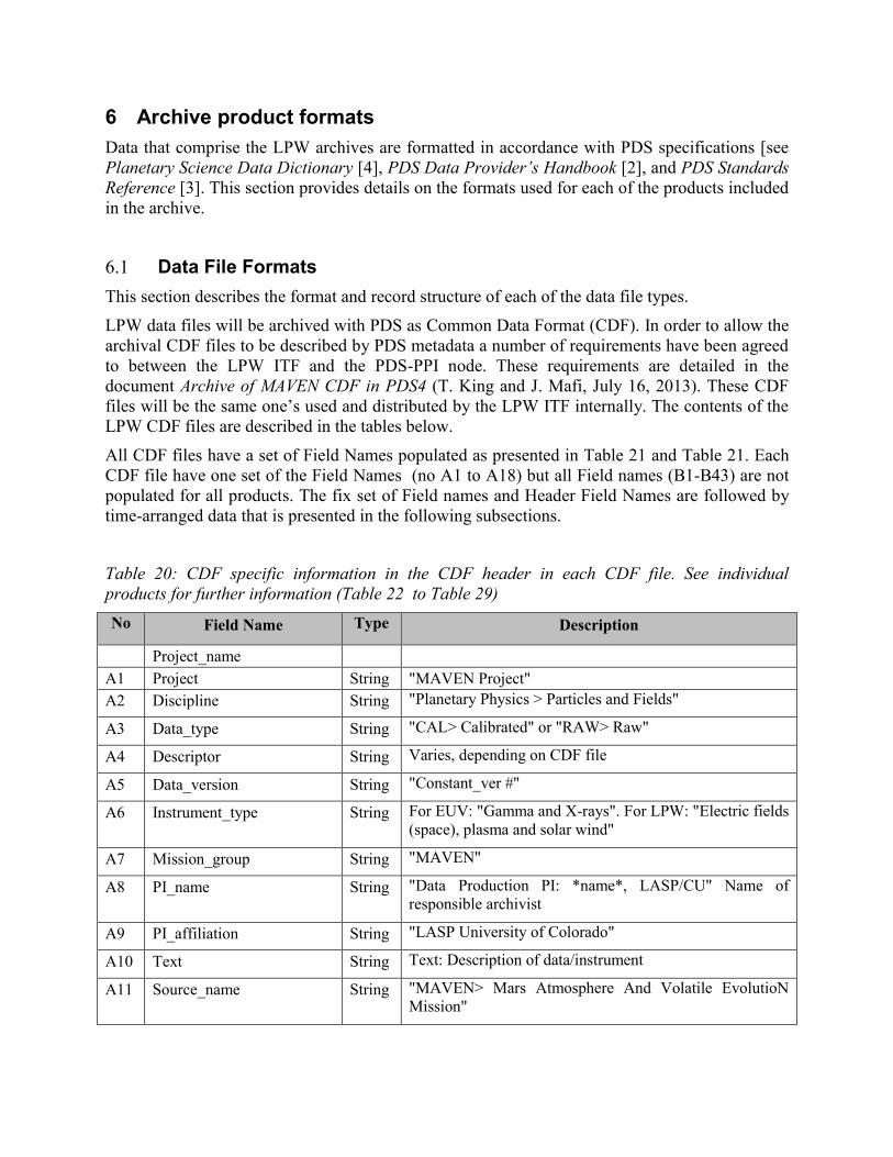
6 Archive product formats

Data that comprise the LPW archives are formatted in accordance with PDS specifications [see

Planetary Science Data Dictionary [4], PDS Data Provider’s Handbook [2], and PDS Standards

Reference [3]. This section provides details on the formats used for each of the products included

in the archive.

6.1 Data File Formats

This section describes the format and record structure of each of the data file types.

LPW data files will be archived with PDS as Common Data Format (CDF). In order to allow the

archival CDF files to be described by PDS metadata a number of requirements have been agreed

to between the LPW ITF and the PDS-PPI node. These requirements are detailed in the

document Archive of MAVEN CDF in PDS4 (T. King and J. Mafi, July 16, 2013). These CDF

files will be the same one’s used and distributed by the LPW ITF internally. The contents of the

LPW CDF files are described in the tables below.

All CDF files have a set of Field Names populated as presented in Table 21 and Table 21. Each

CDF file have one set of the Field Names (no A1 to A18) but all Field names (B1-B43) are not

populated for all products. The fix set of Field names and Header Field Names are followed by

time-arranged data that is presented in the following subsections.

Table 20: CDF specific information in the CDF header in each CDF file. See individual

products for further information (Table 22 to Table 29)

No Field Name Type Description

Project_name

A1 Project String "MAVEN Project"

A2 Discipline String "Planetary Physics > Particles and Fields"

A3 Data_type String "CAL> Calibrated" or "RAW> Raw"

A4 Descriptor String Varies, depending on CDF file

A5 Data_version String "Constant_ver #"

A6 Instrument_type String For EUV: "Gamma and X-rays". For LPW: "Electric fields

(space), plasma and solar wind"

A7 Mission_group String "MAVEN"

A8 PI_name String "Data Production PI: *name*, LASP/CU" Name of

responsible archivist

A9 PI_affiliation String "LASP University of Colorado"

A10 Text String Text: Description of data/instrument

A11 Source_name String "MAVEN> Mars Atmosphere And Volatile EvolutioN

Mission"

No Field Name Type Description

A12 Generated_by String LPW team LASP CU Boulder

A13 Rules_of_use String Web-link

A14 Acknowledgement String Instructions

A15 Dervin String If equation used, information about the data processing

A16 Sig_digits String Number of significant digits

A17 SI_conversion String Unit conversion

A18 Catdesc String Information of the product

A19 x_Catdesc String Information of the x-variable

A20 y_Catdesc String Information of the y-variable

A21 v_Catdesc String Information of the v-variable

A22 dy_Catdesc String Information of the dy-variable (uncertainty/error)

A23 dv_Catdesc String Information of the dv-variable (uncertainty/error/range)

A24 flag_Catdesc String Information of the flag-variable (quality flag)

A25 Display_type String Time series

A26 Var_notes String Information of the product

A27 x_var_notes String Information of the x-variable

A28 y_var_notes String Information of the y-variable

A29 v_var_notes String Information of the v-variable

A30 dy_var_notes String Information of the dy-variable (uncertainty/error)

A31 dv_var_notes String Information of the dv-variable (uncertainty/error/range)

A32 flag_var_notes String Information of the flag-variable (quality flag)

A33 xfieldname String Information of the x-variable

A34 xfieldname String Information of the y-variable

A35 yfieldname String Information of the v-variable

A36 vfieldname String Information of the dy-variable (uncertainty/error)

A37 dyfieldname String Information of the dv-variable (uncertainty/error/range)

A38 dvfieldname String Information of the flag-variable (quality flag)

A39 flagfieldname String Information of the x-variable

A40 fillval Float NaN is used as fill

A41 form_ptr String CDF_float

A42 labaxis String Label of the product

A43 Monoton String "INCREASE"

No Field Name Type Description

A44 Scalemin Float Scalemin: min of data.y

A45 Scalemax Float Scalemin: max of data.y

A46 Var_type String Data

Table 21: LPW Header information that exists in each CDF file but might not always be used.

See the individual products which fields are used (Table 22 to Table 29)

No Header Field

Name Type Description

B1 generated_date String "Gives the date and time the data was processed and the

CDF file was created

Time of the individual processing routines separated by #

B2 t_epoch Double What zero time the spacecraft clock is correlated too.

B3 Time_start Double Array The first data packet presented with different clocks TBR

B4 Time_end Double Array The last data packet presented with different clocks TBR

B5 Time_Field String Array Description of the different clocks used TBR

B6 SPICE_kernel_vers

ion

String SPICE Kernel version

B7 SPICE_kernel_flag String If SPICe kernel was used

B8 Flag_info String Normally flag represent ‘confidence level’ if not stated

differently. 0 no confidence at all.

Can be used for aperture open/close etc.

B9 Flag_source String Contain information of what is considered when the flag is

created (such as sc-attitude)

B10 L0_datafile String Gives the name of the L0 file used.

B11 cal_vers String Gives the calibration file version

B12 cal_y_const1 String Fixed convert information from measured binary values to

physical units, variables from ground testing and design

B13 cal_y_const2 String Fixed convert information from measured binary values to

physical units, variables from space testing

B14 cal_datafile String If one or more calibration files has been used the file names

is located here (file names of the calibration files included

dates and version number of when the are created)

B15 cal_source String Information of what has been considered in the data

production (sc attitude, other instruments etc)

B16 xsubtitle String Units

B17 ysubtitle String Units

B18 cal_v_const1 String Fixed convert information from measured binary values to

physical units, variables from ground testing and design

B19 cal_v_const2 String Fixed convert information from measured binary values to

physical units, variables from space testing

B20 zsubtitle String Units

No Header Field

Name Type Description

- Blank intentionally – a jump in the numbering

B30 char_size String Suggested information for plotting purposes.

B31 xtitle String Suggested information for plotting purposes.

B32 ytitle string Suggested information for plotting purposes.

B33 yrange Float array Suggested information for plotting purposes.

B34 ystyle Integer Suggested information for plotting purposes.

B35 ylog Integer Suggested information for plotting purposes.

B36 ztitle String Suggested information for plotting purposes.

B37 zrange Float array Suggested information for plotting purposes.

B38 zlog Integer Suggested information for plotting purposes.

B39 spec Integer Plotting option, Data type (spectrogram = 1)

B40 labels String Array When different data sources and products are combined in

the y-filed for the CDF file, this fields provide the

information of in which order the products are written

B41 colors Integer Array Suggested information for plotting purposes.

B42 labflag Integer Suggested information for plotting purposes.

B43 noerrorbars Integer Suggested information for plotting purposes.

B44 psym Integer Suggested symbol

B45 no_interp Integer Suggested interpretation for spectra

6.1.1 Raw file data structure

LPW raw data files will be archived with PDS as Common Data Format (CDF). The contents of

the LPW raw CDF files are described in Table 22.

This information of the raw data files urn:nasa:pds:maven.lpw.raw are self documented to some

extent. Each recorded instrument packet is stored in the CDF-file with the spacecraft clock time

stamp. The context of each packet is described in the LPW Header Labels (no 40 in Table 21).

Table 22: Contents for lpw.raw data files.

Field Name Product Name Type Description

A1-A46

B1-B12

B30-B34

LPW_header The information for the header provided in the rows

presented in Table 21. One element per file

x TIME DOUBLE Spacecraft clock taken from each packet header

y RAW INFO FLOAT The RAW information from each packet. The

information in the packet is described by the Field

Name given in Row B40 in Table 21

6.1.2 Calibrated data file structure

LPW calibrated data files will be archived with PDS as Common Data Format (CDF). The

contents of the LPW CDF files are described in Table 21 to Table 26.

Table 23: Contents for lpw.calibrated:data.mgr.sc_pot data file.

Field Name Product Name Type Description

A1-A46,

B1-B12,

B15-B17

B30-B34,

B43

LPW_header The information for the header provided in the rows

presented in Table 21. One element per file

x TIME_UNIX DOUBLE Unix time for this data record, one element per

measurement (sc_pot)

y SC_POT FLOAT Spacecraft potential, one element per time step

dy SC_POT_ERR FLOAT The uncertainty of the measured value. Same number

of elements as sc_pot.

flag SC_POT_FLAG FLOAT A quality flag for each time step

Table 24: Contents for lpw.calibrated:data.w.e12, lpw.calibrated:data.w.e12burstlf,

lpw.calibrated:data.w.e12burstmf, and lpw.calibrated:data.w.e12bursthf data files.

Field Name Product Name Type Description

A1-A46

B1-B12,

B15-B17

B30-B34,

B43

LPW_header The information for the header provided in the rows

presented in Table 21, One element per file

x TIME_UNIX DOUBLE Unix time for this data record, one element per

measurement (W_E12)

y W_E12 FLOAT Electric field measurement, one element per time step

dy W_E12_ERR FLOAT The uncertainty of the measured value. Same number

of elements as W_E12.

flag W_E12_FLAG FLOAT A quality flag for each time step

Table 25: Contents for lpw.calibrated:data.w.specact and lpw.calibrated:data.w.specpas data

files.

Field Name Product Name Type Description

A1-A46

B1-B20

B30-B39

LPW_header The information for the header provided in the rows

presented in Table 21, One element per file

x TIME_UNIX DOUBLE Unix time for this data record, one element per spectra

(SPEC)

y SPEC FLOAT The electric field power for 200 (TBD) frequency bins

for each time step.

v FREQ FLOAT The center frequency of each 200 (TBD) frequency

bin for the respective value in SPEC one element per

file Same number of elements as SPEC.

dy SPEC_ERR FLOAT The uncertainty of the electric field power weighted

with the spacecraft attitude for each frequency step

and time. Same number of elements as SPEC.

dv FREQ_WIDTH FLOAT Provide information of the frequency width Same

number of elements as SPEC.

flag SPEC_FLAG FLOAT A quality flag for each time step

Table 26: Contents for lpw.calibrated:data.lp.iv data file.

Field Name Product Name Type Description

A1-A46

B1-B20

B30-B39

LPW_header The information for the header provided in the rows

presented in Table 21, One element per file

x TIME_UNIX DOUBLE Unix time for this data record, one element per sweep

(LP_I)

y LP_I FLOAT The measured current from the probe as the potential

of the probe is changed in the time order of the sweep,

128 points for each time step

v LP_V FLOAT The sweeping potential in the time order of the sweep,

128 points for each time step. Same number of

elements as LP_I.

dy LP_I_ERR FLOAT The uncertainty in the measured current, 128 points

for each time step (or a % value TBD), 128 points for

each time step. Same number of elements as LP_I.

dv LP_V_ERR FLOAT The uncertainty in the applied potential, 128 points,

one per file (or do we need one for each time step

TBD). Same number of elements as LP_I.

flag LP_IV_FLAG FLOAT A quality flag for each time step

6.1.3 Derived data file structure

LPW derived data files will be archived with PDS as Common Data Format (CDF). The contents

of the LPW CDF files are described in Table 21 and Table 28 to Table 29.

Table 27: Contents for lpw.derived:data.w.n data files.

Field Name Product Name Type Description

A1-A46

B1-B12,

B15-B17

B30-B34,

B43

LPW_header The information for the header provided in the rows

presented in Table 21, One element per file

x TIME_UNIX DOUBLE Unix time for this data record, one element per

measurement (W_N)

y W_N FLOAT The derived electron density from the Langmuir line,

one element per time step, data only when plasma line

is observed

dy W_N_ERR FLOAT ‘Quality’ of how easy the Langmuir line was

identified. Same number of elements as W_N.

flag SPEC_FLAG FLOAT A quality flag for each time step

Table 28: Contents for lpw.derived:data.lp.nt data files.

Field Name Product Name Type Description

A1-A46

B1-B12,

B15-B17

B30-B34,

B40-B43

LPW_header The information for the header provided in the rows

presented in Table 21, One element per file

x TIME_UNIX DOUBLE Unix time for this data record, one element per

measurement (LP_N_T)

y LP_N_T FLOAT Presently planned [‘T1’, ’n1’,’T2’,’n2’,’t_tot’,’n_tot’

’sc_pot’, ’Photo_e_I’,’euv’] The quantities derived

from line fits. The fit can either be for a single

maxwellian of a double maxwellina. The n1 & n2 and

T1 and T2 provide this information.

dy LP_N_T_ERROR FLOAT The uncertainty in all of the fitted parameters.

flag LP_N_T_FLAG FLOAT The quality of the measured IV-measurement. One

element per time step.

Table 29: Contents for lpw.derived:data.mgr.exb data file.

Field Name Product Name Type Description

A1-A46

B1-B12,

B15-B17

B30-B34,

B40-B43

LPW_header The information for the header provided in the rows

presented in Table 21. One element per file

x TIME_UNIX DOUBLE Unix time for this data record, one element per 256

sec (TBD)

y S_E_B FLOAT Presently planned information [‘S’, ‘B’, ‘dB’,’dE’].

The 1-D smoothed electric field measurement

presented in MSO coordinate system, each quantity is

describe with three components (x, y, z)

dy S_ERR FLOAT The uncertainty of the four different quantities

flag S_FLAG FLOAT Indicating how turbulent the low frequency electric

and magnetic field that was used for each averaged

data point (alternative, how much the magnetic field

was rotating during one point), one element per time

step

6.2 Document Product File Formats

LPW will provide the raw data and the calibrated/derived data in CDF formats. The processing

from raw to calibrated/derived is documented with the archiving ASCII files with the IDL

program scripts. The SIS document (this document) will be archived in word-format (PDF?

TBR).

6.3 PDS Labels

PDS labels are ASCII text files written, in the eXtensible Markup Language (XML). All product

labels are detached from the digital files (if any) containing the data objects they describe (except

Product_Bundle). There is one label for every product. Each product, however, may contain one

or more data objects. The data objects of a given product may all reside in a single file, or they

may be stored in multiple separate files. PDS4 label files must end with the file extension “.xml”.

The structure of PDS label files is governed by the XML documents described in Section 6.3.1.

6.3.1 XML Documents

For the MAVEN mission PDS labels will conform to the PDS master schema based upon the

1.1.0.1 version of the PDS Information Model for structure, and the 1.1.0.1 version of the PDS

schematron for content. By use of an XML editor these documents may be used to validate the

structure and content of the product labels.

The PDS master schema and schematron documents are produced, managed, and supplied to

MAVEN by the PDS. In addition to these documents, the MAVEN mission has produced

additional XML documents which govern the products in this archive. These documents contain

attribute and parameter definitions specific to the MAVEN mission. A full list of XML

documents associated with this archive is provided in Table 14. A list of the XML documents

associated with this archive is included in this document in the XML_Schema collection section

for each bundle.

Examples of PDS labels required for the LPW archive are shown in Appendix C (bundle

products), Appendix D (collection products), and Appendix E (basic products).

6.4 Delivery Package

Data transfers, whether from data providers to PDS or from PDS to data users or to the deep

archive, are accomplished using delivery packages. Delivery packages include the following

required elements:

1. The package which consists of a compressed bundle of the products being transferred.

2. A transfer manifest which maps each product’s LIDVID to the physical location of the

product label in the package after uncompression.

3. A checksum manifest which lists the MD5 checksum of each file included in the package

after uncompression.

LPW archive delivery packages (including the transfer and checksum manifests) for delivery to

PDS are produced at the MAVEN SDC.

6.4.1 The Package

The directory structure used in for the delivery package is described in the Appendix in Section

F.1. Delivery packages are compressed using either [zip, or tar/gzip – SDC text] and are

transferred electronically using the ssh protocol.

6.4.2 Transfer Manifest

The “transfer manifest” is a file provided with each transfer to, from, or within PDS. The transfer

manifest is external to the delivery package. It contains an entry for each label file in the

package, and maps the product LIDVID to the file specification name for the associated

product’s label file. Details of the structure of the transfer manifest are provided in Section F.2.

The transfer manifest is external to the delivery package, and is not an archive product. As a

result, it does not require a PDS label.

6.4.3 Checksum Manifest

The checksum manifest contains an MD5 checksum for every file included as part of the

delivery package. This includes both the PDS product labels and the files containing the digital

objects which they describe. The format used for a checksum manifest is the standard output

generated by the md5deep utility. Details of the structure of the checksum manifest are provided

in section F.3.

The checksum manifest is external to the delivery package, and is not an archive product. As a

result, it does not require a PDS label.

Appendix A Support staff and cognizant persons

Table 30: Archive support staff

LPW team

Name Address Phone Email

Dr. Laila

Andersson

3665 Discovery Drive 303 492 1689 Laila.andersson@lasp.colorado.edu

UCLA

Name Address Phone Email

Dr. Steven Joy

PPI Operations Manager

IGPP, University of California

405 Hilgard Avenue

Los Angeles, CA 90095-1567

USA

+001 310

825 3506

sjoy@igpp.ucla.edu

Mr. Joseph Mafi

PPI Data Engineer

IGPP, University of California

405 Hilgard Avenue

Los Angeles, CA 90095-1567

USA

+001 310

206 6073

jmafi@igpp.ucla.edu

Appendix B Naming conventions for MAVEN science data files

This section describes the naming convention used for science data files for the MAVEN

mission.

Raw (MAVEN Level 0): This is not used for LPW data

mvn_<inst>_<grouping>_l0_< yyyy><mm><dd>_v<xxx>.dat

Level 0b, 1a, 1b, 2, 3+:

mvn_<inst>_<level>_<descriptor>_<yyyy><mm><dd>T<hh><mm><ss>_v<xx>_r<yy>.<ext>

Code Description

<inst> 3-letter instrument ID

<grouping> Three-letter code: options are all, svy, and arc for all data, survey data, and

archive data respectively. Primarily for PF to divide their survey and archive

data at Level 0.

<yyyy> 4-digit year

<mm> 2-digit month, e.g. 01, 12

<dd> 2-digit day of month, e.g. 02, 31

<hh> 2-digit hour, separated from the date by T. OPTIONAL.

<mm> 2-digit minute. OPTIONAL.

<ss> 2-digit second. OPTIONAL.

v<xx> 2-digit CDF file structure version.

r<yy> 2-digit the revision version of the data product

<descriptor> A description of the data. Defined by the creator of the dataset. There are no

underscores in the value.

.<ext> File type extension: .fits, .txt, .cdf, .png LPW will only use CDF

<level> A code indicating the MAVEN processing level of the data, LPW will use for

archiving purpose the following levels: raw, calib, merged, derived, and

modeled. L0b, L1a and L1b are in the process stored for the team, since they

are temporary, incomplete, they are not archived at PDS.

Instrument name <instrument>

IUVS iuv

NGIMS ngi

LPW lpw

EUV euv

MAG mag

SEP sep

SWIA swi

SWEA swe

STATIC sta

PF package pfp

Appendix C Sample Bundle Product Label

This section provides a sample bundle product label.

Appendix D Sample Collection Product Label

This section provides a sample collection product label.

Appendix E Sample Data Product Labels

This section provides sample product labels for the various data types described in this

document.

Appendix F PDS Delivery Package Manifest File Record Structures

The delivery package includes two manifest files: a transfer manifest, and MD5 checksum

manifest. When delivered as part of a data delivery, these two files are not PDS archive products,

and do not require PDS labels files. The format of each of these files is described below.

F.1 Transfer Package Directory Structure

[Insert a description of the directory structure contained in the delivery package.]

F.2 Transfer Manifest Record Structure

The transfer manifest is defined as a two field fixed-width table where each row of the table

describes one of the products in the package. The first field defines the LIDVID of each product

in the package. The second field defines the file specification name of the corresponding product

label in the package. The file specification name defines the name and location of the product

relative to the location of the bundle product.

F.3 Checksum Manifest Record Structure

The checksum manifest consists of two fields: a 32 character hexadecimal (using lowercase

letters) MD5, and a file specification from the root directory of the unzipped delivery package to

every file included in the package. The file specification uses forward slashes (“/”) as path

delimiters. The two fields are separated by two spaces. Manifest records may be of variable

length. This is the standard output format for a variety of MD5 checksum tools (e.g. md5deep,

etc.).