Marriage and Wages

Elena Bardasi and Mark Taylor

ISER Working Papers Number 2005-1

Institute for Social and Economic Research The Institute for Social and Economic Research (ISER) specialises in the production and analysis of longitudinal data. ISER incorporates the following centres: • ESRC Research Centre on Micro-social Change. Established in 1989 to identify, explain, model

and forecast social change in Britain at the individual and household level, the Centre specialises in research using longitudinal data.

• ESRC UK Longitudinal Centre. This national resource centre was established in October 1999 to

promote the use of longitudinal data and to develop a strategy for the future of large-scale longitudinal surveys. It was responsible for the British Household Panel Survey (BHPS) and for the ESRC’s interest in the National Child Development Study and the 1970 British Cohort Study

• European Centre for Analysis in the Social Sciences. ECASS is an interdisciplinary research

centre which hosts major research programmes and helps researchers from the EU gain access to longitudinal data and cross-national datasets from all over Europe.

The British Household Panel Survey is one of the main instruments for measuring social change in Britain. The BHPS comprises a nationally representative sample of around 5,500 households and over 10,000 individuals who are reinterviewed each year. The questionnaire includes a constant core of items accompanied by a variable component in order to provide for the collection of initial conditions data and to allow for the subsequent inclusion of emerging research and policy concerns. Among the main projects in ISER’s research programme are: the labour market and the division of domestic responsibilities; changes in families and households; modelling households’ labour force behaviour; wealth, well-being and socio-economic structure; resource distribution in the household; and modelling techniques and survey methodology. BHPS data provide the academic community, policymakers and private sector with a unique national resource and allow for comparative research with similar studies in Europe, the United States and Canada. BHPS data are available from the Data Archive at the University of Essex http://www.data-archive.ac.uk Further information about the BHPS and other longitudinal surveys can be obtained by telephoning +44 (0) 1206 873543. The support of both the Economic and Social Research Council (ESRC) and the University of Essex is gratefully acknowledged. The work reported in this paper is part of the scientific programme of the Institute for Social and Economic Research.

Acknowledgement: This paper has benefited with helpful discussions with Leslie Stratton, and comments received from participants at the XVIII Annual Conference of the European Society for Population Economics in Bergen, Norway. The support of the Economic and Social Research Council (UK), and the University of Essex is gratefully acknowledged. BHPS data are available from the Data Archive at the University of Essex.

Readers wishing to cite this document are asked to use the following form of words:

Familyname, Firstname (February 2005) ‘Title of Working Paper’, Working Papers of the Institute for Social and Economic Research, paper 20055-1. Colchester: University of Essex.

For an on-line version of this working paper and others in the series, please visit the Institute’s website at: http://www.iser.essex.ac.uk/pubs/workpaps/

Institute for Social and Economic Research University of Essex Wivenhoe Park Colchester Essex CO4 3SQ UK Telephone: +44 (0) 1206 872957 Fax: +44 (0) 1206 873151 E-mail: iser@essex.ac.uk Website: http://www.iser.essex.ac.uk

January 2005 All rights reserved. No part of this publication may be reproduced, stored in a retrieval system or transmitted, in any form, or by any means, mechanical, photocopying, recording or otherwise, without the prior permission of the Communications Manager, Institute for Social and Economic Research.

ABSTRACT

This work investigates the commonly observed relationship between marriage and wages among men in Britain using panel data covering the 1990s. We explicitly test several hypotheses developed in the literature to explain this relationship, including the household division of labour and specialisation, differential rates of human capital formation, employer favouritism, and self-selection. After accounting for individual-specific time-invariant effects, and a wide range of individual, household, job and employer related characteristics, we find a small but statistically significant premium remains that can be attributed to productivity differences. Our estimates provide evidence for the existence of a large selection effect into marriage based on both observable and unobservable characteristics that are positively correlated with wages (consistent with employers using marriage as a positive signal), and also evidence in support of the specialisation hypothesis.

NON-TECHNICAL SUMMARY

Much research in applied economics has commented on the advantages associated with marriage. Marriage has been found to have positive effects both on reported levels of happiness and health. In addition, a male marriage premium is a common finding in wage equations, indicating that marriage is associated with higher wages for men. However, there is the question of causality – does marriage itself make men more productive and therefore increase their earnings? Or alternatively do more productive, higher earning men get married? If marital status is genuinely productivity enhancing, then changes in the marital status composition of the workforce will affect productivity. If there are no productivity effects of marriage, then changes in the marital status composition of the workforce will have no impact on economic output. In this paper we investigate in detail the presence and causes of a marriage wage premium among men in Britain using panel data from the first eleven years of the British Household Panel Survey (BHPS), covering the period 1991–2001. We explicitly test several hypotheses developed in the literature to explain the relationship between marriage and wages. By using panel data we are able to allow for possible correlations between unobserved characteristics, marriage and wages. Failure to do so will bias the coefficient of interest – some of the returns attributed to marriage may actually be returns to some unobserved qualities correlated with marriage. If so, the observed wage premium associated with marriage largely reflects unobserved individual characteristics that are also valued by the employer. Our work provides new evidence on the existence and causes of the marriage wage premium among married men in Britain by using a long run of panel data. Cross-sectional analysis yields a wage premium for married men of about 15%, consistent with much of the previous literature. Using panel data and panel data methods, we find that this premium falls dramatically, indicating that about three-quarters of the observed premium in cross-sectional analysis is caused by unobserved individual heterogeneity and/or selection effects. Married men have unobserved characteristics that are also correlated with wages. Our results are consistent with the hypothesis that employers use marriage as a signal – a large proportion of the marriage premium is due to unobservable characteristics that are valued both by wives and by employers, such as motivation, loyalty, dependability and determination. Nevertheless, a relatively small but statistically significant marriage premium remains even when allowing for a wide range of individual, household, job and employer-related characteristics and time invariant individual specific unobservable effects. Our preferred panel estimates indicate the size of this premium increases with the number of domestic chores for which the spouse is mostly responsible, and falls with the wife’s working hours. The relative sizes of the coefficients suggest that a married man whose wife does not work but whose wife is mostly responsible for four domestic chores enjoys a wage premium of about 4% relative to a single never married man. However this premium almost disappears if the wife also works 40 hours per week in the labour market. We show that the effects of the hours worked and domestic chores carried out by the wife are genuine, and not due to the potential endogeneity of the wife’s decision to work. Our estimates therefore provide some evidence in favour of the specialisation explanation for the enhanced productivity of married men.

1

Introduction

Much research in applied economics has commented on the advantages associated with

marriage. Marriage has been found to have positive effects both on reported levels of

happiness (Myers 1999; Diener et al 2000; Stutzer and Frey 2003; Blanchflower and Oswald

2004) and health (Ross et al 1990; Waite and Gallagher 2000; Wilson and Oswald 2002; Ribar

2004). In addition, a male marriage premium is a common finding in wage equations,

indicating that marriage is associated with higher wages for men (Korenman and Neumark

1991; Schoeni 1995; Loh 1996; Chun and Lee 2001; Ribar 2004). However, there is the

question of causality – does marriage itself make men more productive and therefore increase

their earnings? Or alternatively do more productive, higher earning men get married? If marital

status is genuinely productivity enhancing, then changes in the marital status composition of

the workforce will affect productivity (Korenman and Neumark 1991). If there are no

productivity effects of marriage, then changes in the marital status composition of the

workforce will have no impact on economic output. In this paper we investigate in detail the

presence and causes of a marriage wage premium among men in Britain using panel data from

the first eleven years of the British Household Panel Survey (BHPS), covering the period

1991–2001. We explicitly test several hypotheses developed in the literature to explain the

relationship between marriage and wages.

Previous research has reported large wage premiums associated with marriage, varying

between 10% and 40% in cross-sectional studies (Korenman and Neumark 1991, Schoeni

1995). Studies that use panel data typically report that this premium is considerably reduced, if

not eradicated altogether, when allowing for individual specific fixed effects (Korenmen and

Newmark 1991; Cornwell and Rupert 1995; Jacobsen and Rayack 1996; Stratton 2002). This

indicates that at least part of the premium is related to unobserved characteristics of the

worker. Studies focussing on men in Britain report a marriage premium ranging from 10% to

14%, although the majority of these use cross-sectional data (Greenhalgh 1980; Schoeni 1995;

Disney and Whitehouse 1996). Exceptions are Joshi and Newell (1989), who use birth cohort

data and report a wage premium of about 10% for married men, and Davies and Peronaci

(1997). The latter study uses data from the first four years of the British Household Panel

Survey, and finds that the size of premium falls dramatically when allowing for time invariant

individual specific effects. We build on this earlier work, having the advantages of access to

2

panel data over a longer period and many more control variables including very rich sets of

individual, employer, and job characteristics.

There are a number of possible explanations for why married men earn should more than their

unmarried counterparts, some of which emerge directly from economies of scale and

specialisation within the family (Becker 1973; 1974; 1991). Marriage facilitates the

specialisation of labour and traditionally results in the husband becoming market intensive.

Increased specialisation in the labour market enhances a man’s productivity that translates into

higher wages. A number of previous studies find evidence in favour of this specialisation

hypothesis (Daniel 1992; Gray 1997; Chun and Lee 2001), while others find evidence against

it (Davies and Peronaci 1997; Loh 1996).

It is possible that marriage creates conditions under which the accumulation of human capital

is more efficient than as an unmarried worker. It may increase the time available to invest in

market specific human capital, or the wife may contribute directly to the husband’s human

capital by supplying a flow of services. US evidence suggests that married men are more likely

to receive work-related training and accumulate human capital at a faster rate (Loh 1996). If

this marriage induced human capital accumulation translates into higher wages and faster wage

growth, then married men will exhibit a wage premium (Nakosteen and Zimmer 1987; Stratton

2002). However, previous evidence suggests that this is not the cause of the marriage

premium among British men (Davies and Peronaci 1997).

A marriage wage premium can also result from employer discrimination, which may or may

not reflect higher productivity. For example, employers may discriminate in favour of married

men not because of higher productivity but because they conform to a social norm that men

should be married and supporting families (Loh 1996; Davies and Peronaci 1997). Employers

may be paternalistic in supporting men with families and may be particularly supportive of men

whose wife does not work in the labour market. Employers may also use marriage as a signal

for higher productivity, as marriage is associated with highly valued unobservable

characteristics such as ability, honesty, loyalty, dependability and determination. The latter has

3

found some empirical support in the US literature (Korenmen and Neumark 1991; Cornwell

and Rupert 1995; Loh 1996).1

A final and related explanation is that the observed marriage wage premium is a statistical

artefact. The positive selection of high wage males into marriage creates an appearance of a

marriage premium in observed earnings (Nakosteen and Zimmer 1987; Gray 1997; Davies and

Peronaci 1997). Men that possess attributes rewarded in the labour market are also valued in

the marriage market – men with wage enhancing unobserved characteristics are selected into

marriage. Again, there are empirical studies that produce evidence both in favour (Nakosteen

and Zimmer 1987; Jacobsen and Rayack 1996; Davies and Peronaci 1997) and against

(Korenmen and Neumark 1991; Chun and Lee 2001) the selection and unobserved

heterogeneity hypothesis.

In this paper, we use panel data to test these various explanations for why the earnings of

married men exceed those of otherwise similar unmarried men. By using panel data we are

able to allow for possible correlations between unobservables, marriage and wages. Failure to

do so will bias the coefficient of interest – some of the returns attributed to marriage may

actually be returns to some unobserved qualities correlated with marriage. If so, the observed

wage premium associated with marriage largely reflects unobserved individual characteristics

that are also valued by the employer. Our work provides new evidence on the existence and

causes of the marriage wage premium among married men in Britain by using a long run of

panel data.

Data

Our analysis uses data from the British Household Panel Survey (BHPS). Since 1991, this has

interviewed on an annual basis a representative sample of 5,500 households containing

approximately 10,000 individuals. These same individuals are re-interviewed each year on a

wide range of subjects including basic demographics, household composition and

circumstances, employment status and recent employment history, job characteristics if

employed, income from all sources and so on. Currently eleven years of data are available,

1 It is also possible that married men, especially those with families, choose jobs with fewer non-monetary benefits but that offer higher wages (Reed and Hartford 1989). We do not test this compensating wage

4

covering the period 1991-2001. The use of panel data is important in our context, as it allows

us to examine how wages of individuals change as they change marital status and to allow for

time invariant unobserved individual specific effects. These may be correlated with both the

probability of marriage and wages and therefore bias the coefficients of interest.

We restrict our analysis to men aged between 18 and 59 (inclusive), who report being in full-

time work as their main status. We select only men who were full respondents and were part

of the core BHPS sample.2 Ethnic minorities, those in the armed forces and those with second

jobs are also excluded. The hourly wage we use as the dependent variable is constructed from

respondents reported usual gross income from their main job and their reported weekly hours

of work.3 This is expressed in real terms, deflated to January 2002 prices.

We focus only on employees, because the inclusion of self-employed workers in our sample is

problematic for several reasons. First, almost one half of the self-employed did not respond to

the earnings question and had their earnings imputed (in contrast to only 7% of employees).4

Second, it is well documented that the self-employed have a tendency to under-report their

earnings. Third, income from self-employment includes returns from both labour and from

physical capital. Fourth, the number of hours worked in a normal week is likely to be more

unreliable for the self-employed than employees.5 Selection based on these criteria (and

dropping observations with missing information) results in a sample of 3656 men contributing

16857 person-year observations.

hypothesis explicitly, but instead control for a wide range of individual, job and employer characteristics that either directly or indirectly capture non-pecuniary compensation. 2 The original core BHPS sample has been boosted at various stages to include, for example, the UK European Household Community Panel sample, and Welsh, Irish and Scottish booster samples. We exclude these booster samples from our analysis. We have also re-estimated our models focusing on men aged less than 40 who are most at risk of marriage. The results from doing so are qualitatively unchanged from those discussed herein. 3 One drawback with the earnings data in the BHPS is that the question about usual earnings asks for gross pay including overtime, bonuses, commission etc, and it is therefore not possible to calculate a measure of ‘basic pay’. We overcome this to some extent by assuming that a wage premium of 50% is received for any paid overtime hours worked by the individual. Our results are robust to varying this assumed overtime rate. 4 We have kept those with imputed earnings in our estimating sub-sample, although our results are robust to their exclusion. 5 An additional complication for the self-employed is that they are allowed to report their earnings either before or after income taxes and other deductions. Although the majority report pre-tax gross earnings, a non-negligible minority report earnings at different stages of the taxation process. Simulations are used to reconstruct gross earnings for this group, but this inevitably introduces measurement error problems.

5

Table 1 presents mean wages by marital status (as recorded at each date of interview) for the

pooled sample over the eleven year period. This indicates that currently married men enjoyed

the highest wages, at £10.75 per hour, followed by men who were divorced, separated or

widowed at £9.83 per hour. Cohabiting men had average wages of £8.97 per hour, and single

men who had never been married had the lowest average wages, of £7.37 per hour. Therefore

the raw descriptive statistics confirm the presence of a wage premium for married men in

Britain of about 46% relative to the single never married, and 23% relative to the currently not

married. Cohabiting men earn 22% more than single never married men, but 17% less than

married men. However, these mean wages do not control for differences in other observable

characteristics (for example, married men are typically older than unmarried ones) nor in

unobservable traits.

Econometric and empirical specification

Wages are assumed to be determined by the following equation:

itiititit MXw εαγβ +++=)ln( [1

]

where itw is the wage of individual i in year t, X is a vector of observable individual,

household, job and employer related characteristics that determine wages, M is the variable

capturing the marital status of the individual, iα captures the unobserved, time-invariant

characteristics of the individual, and itε is random error. Estimating this equation by OLS

implicitly assumes that iα is zero, and therefore uncorrelated with both itw and X. However

this is unrealistic in the present context, as X includes measures of education and job tenure

that are correlated with, for example, any unobserved ability captured in iα . Furthermore, if

this unobserved individual specific effect is also correlated with the probability of being

married, then the main coefficient of interest, γ , will be biased. In particular, the selection of

men with unobserved wage-enhancing characteristics into marriage implies a correlation

between M and iα , and results in an upwardly biased estimate of γ . Panel data allow us to

overcome these potential problems of endogeneity in two ways. The first is to estimate [1]

using ‘within-group’ fixed-effects, which is equivalent to the simple OLS estimation in which

the variables are defined as deviations from their individual means over the panel period.

Therefore the model to be estimated becomes:

6

itiitiitiit vMMXXww +−+−=− γβ )()()ln()ln( [2

]

This removes the individual fixed-effect iα and has been the standard approach in previous

investigations of the marriage wage premium that use longitudinal data from the US

(Korenmen and Neumark 1991; Cornwell and Rupert 1995; Jacobsen and Rayack 1996).

Although clearly preferred to the OLS estimator, this procedure does not correct for bias due

to unobservable characteristics that are correlated with marital status but that vary over time.

An alternative approach is to treat the unobserved effect iα as random, and estimate [1] using

random effects. The limitation of this approach is that it assumes that the unobserved

individual specific effect, iα , is independent of the observed characteristics in X and M. This is

particularly problematical in our context, as we expect more able and motivated men to be

both more likely to be married and to earn higher wages. Therefore the estimated coefficient

γ will remain upwardly biased. To avoid this problem, we relax the assumption that iα is

independent of the time varying characteristics in X and M. Following Chamberlain (1984) we

model the dependence between iα and the observable characteristics by assuming that the

regression function of iα is linear in the means of all the time varying covariates. This can be

written:

iiii MX ηα +∂+∂+∂= 210 [3

]

Where iX and iM refer to the vector of means of the time varying covariates for individual i

over time. Equation [1] therefore becomes:

itiiiititit MXMXw ωηγβ ++∂+∂++= 21)ln( [4

]

This is equivalent to the random effects regression with additional regressors iX and iM .

These panel data estimation procedures overcome some of the problems associated with self-

selection and endogeneity that might otherwise result in a spurious positive coefficient on the

married variable and the misleading conclusion that a marriage wage premium exists.

Another source of selection bias arises if selection into marriage depends on wage growth. In

this case, changes in wages and marital status are interdependent and the estimated coefficient

7

on the married variable will be biased upwards if high wage growth increases the probability of

marriage (Ginther and Zavodny 2001). The standard approach to address this kind of

endogeneity is instrumental variables estimation. This requires at least one variable that is

correlated with marital status but uncorrelated with the error term in the wage equation. We

present and discuss the results from all three estimation procedures below.

Our basic empirical specifications include a wide range of individual, household, job and

employer related characteristics that have previously been shown in the literature to determine

wages. All specifications include, for example, variables to capture whether the man is an

immigrant, registered disabled, has a limiting health condition, region of residence, age and age

squared, highest educational qualification, recent employment history, industry, sector of

employment, establishment size, weekly hours worked, number of paid overtime hours, trade

union coverage and membership, place of work, elapsed job tenure, occupation and year

indicators. We also include a range of variables that may identify non-pecuniary compensation

such as the opportunity for regular promotion, regular pay increments, bonus payments or

profit sharing, and contributing to an occupational pension scheme. In addition we estimate a

number of different empirical specifications in order to test the various potential hypotheses

explaining the presence of the marriage wage premium.

Hypothesis testing

Specialisation

The first hypothesis we consider is specialisation. This hypothesis derives directly from Becker

(1991), in that marriage allows the husband and wife to specialise in either market or domestic

production. Traditionally, the husband supplies his labour to the market and this household

division of labour allows him to allocate greater effort to this. His productivity and his wage

increase as a result. This hypothesis has a number of implications that can be directly tested

with our data. In particular, if the marriage wage premium is due to specialisation then:

1. Men in cohabiting unions should exhibit a similar premium. We expect the same

specialisation to occur irrespective of whether the couple are married or cohabiting,

although given the less stable nature of cohabitation we might expect greater specialisation

in marriage. The BHPS data allow us to identify whether a man is cohabiting at each date

8

of interview, and a positive coefficient on this variable (relative to the single never-

married) would support the specialisation hypothesis.

2. Any wage gains from marriage should disappear when a marriage dissolves, as any benefits

of specialisation will be lost (Davies and Peronaci 1997). Therefore divorced, separated or

widowed men (who are not cohabiting) should not enjoy any wage premium. Again, the

BHPS data allow us to identify such men, and a non-positive coefficient on this variable

(relative to the single never-married) would support the specialisation hypothesis.

3. The wage premium should decline with the wife’s working hours (Loh 1996; Davies and

Peronaci 1997). This is because the degree of specialisation in the household declines as

the hours worked by the wife increases. We can explicitly test this by including wife’s

weekly working hours as an additional explanatory variable in the wage regressions, and a

negative coefficient on this variable would support the specialisation hypothesis.

4. The wage premium should increase with the number of domestic chores for which the wife

is responsible. The degree of specialisation is higher in households where the wife is

responsible for a larger proportion of domestic work, such as buying the groceries,

cooking, cleaning and washing and ironing, and this should be reflected in the size of the

marriage premium for the husband. BHPS data contain information on which partner in

couple households is mainly responsible for a range of domestic chores, allowing us to test

for this explicitly. In particular married and cohabiting men and women were asked:

“Could you please say who mostly does these household jobs here? Is it mostly yourself, mostly your spouse/partner, or is the work shared equally? (1) Grocery shopping; (2) Cooking; (3) Washing and ironing; (4) Cleaning/hoovering.”

For each married or cohabiting man, we have added together the number of chores for

which the spouse/partner is mostly responsible (taking a value between 0 and 4) and use

this as a direct measure of the degree of specialisation in the household.6 A positive

coefficient on this variable would support the specialisation hypothesis.

Human capital accumulation

6 This takes the value 0 if the man is not married or cohabiting. This variable was not collected at 1992 and 1993, and hence the sample sizes are smaller in this specification. We have also experimented with including the number of chores for which the man is mostly responsible. This was statistically insignificant in all specifications.

9

The second, and related, hypothesis to explain the marriage wage premium among men is

human capital accumulation. There are a number of different ways in which a wife can

contribute to her husband’s human capital. Traditionally, by fulfilling domestic chores and

supplying a flow of services, she allows the husband more time to develop his work-related

skills and knowledge and to build better social relations and networks that pay off in terms of

promotions and faster wage growth. She may also provide funding for training, or provide

more direct market-related information on job vacancies etc. Again, this human capital

argument has a number of implications that can be tested directly using BHPS data. In

particular, if the marriage wage premium is due to human capital accumulation then:

1. As with the specialisation hypothesis, cohabiting as well as married men should enjoy a

wage premium.

2. The size of the premium should be lower if the wife also works, for reasons akin to those

in the specialisation hypothesis.

3. We would expect the wage premium to increase with the elapsed duration of the marriage.

The more time the husband has been married, the more time he has had to improve his

human capital. Therefore a positive coefficient on the elapsed duration of marriage variable

would support the human capital hypothesis.7

4. Unlike under the specialisation hypothesis, the premium should be retained to some extent

on marital dissolution (Davies and Peronaci 1997). This is because although no longer

married, the man has accumulated human capital while married and this should still be

reflected in his wage. Therefore a positive coefficient on a variable indicating whether the

man is divorced, separated or widowed (relative to the single never-married) would

support the human capital hypothesis.

5. The presence of children in the household reduces the time available to the wife to

augment her husband’s human capital, and thus should lower the wage premium (Davies

and Peronaci, 1997). Therefore a negative coefficient on the number of children in the

household would support the human capital hypothesis.

Employer discrimination

7 Information on marriage duration in the BHPS was originally collected in a marital and fertility history in 1992. To avoid dropping men who were not interviewed in 1992, we have constructed a missing marriage

10

The third explanation used to explain the wage premium for married men concerns employer

discrimination in favour of married men. There are two potential reasons for this

discrimination. The first is that employers favour married men as they conform to social

expectations, although there may not be any actual productivity differences.8 If this employer

paternalism is the cause of the marriage wage premium then:

1. We would expect men with children to enjoy a larger premium than those without children

as the presence of children reinforces the social expectation of the marriage institution.

Therefore a positive coefficient on the number of children indicator would support the

employer discrimination hypothesis.

2. According to this hypothesis, it is the state of being married rather than the duration of the

marriage that is important, and therefore there should be no relationship between elapsed

duration of the marriage and the wage received.

The second reason for employer discrimination in favour of married men is that employers

might use marriage as a signal of particular, highly valued unobserved characteristics that are

productivity enhancing, such as commitment, motivation, honesty etc. If this signalling is the

cause of the marriage wage premium, then the marriage wage premium should disappear in

models that allow for time invariant individual specific effects.

In the next section we present and discuss the results from various model specifications that

explicitly test these hypotheses.

Results

Table 2, 3 and 4 present the results from our regressions, with the natural log of hourly wages

as the explanatory variable and marital status and related variables among the explanatory

variables. Each column shows the results from a different specification, testing the various

hypotheses described above. In particular, specification [1] shows the results when marital

duration indicator which has been included in all relevant specifications. There are 2015 person-year observations with missing marriage duration (12% of the sample). 8 A further implication of the employer favouritism hypothesis that we do not test here is that the marriage wage premium should not be detected for the self-employed (Loh 1996). As an experiment, and despite our reservations listed previously, we have estimated models using a sample including self-employed workers. Despite trying various different model specifications, we did not find any marriage premium for self-employed men. This can be interpreted as evidence in support of the hypothesis that employers favour married men.

11

status is measured by including a variable indicating whether or not the man is married.

Specifications [2] and [3] introduce additional variables indicating whether the man is

cohabiting, and whether he is divorced, separated or widowed. Specification [4] adds a

variable measuring the weekly hours of work of the spouse (which takes the value zero if the

man is not married or cohabiting)9, while specification [5] adds the elapsed duration of the

marriage (measured in years).10 Specification [6] introduces a variable that measures the

number of children in the family, while the final specification, specification [7], introduces the

variable that measures the number of domestic chores for which the spouse is mainly

responsible.

OLS

For the time being, we ignore issues surrounding potential selection effects and endogeneity,

and estimate models using OLS. Focusing initially on the coefficients on the ‘married’ variable,

our results are consistent with previous studies using British data. We find a positive and

significant effect of marriage on wages, resulting in a wage premium of between 9% and 18%.

These estimated premia are much lower than those observed in the raw data, indicating

selection into marriage based on observable characteristics – married men have observable

characteristics that are also associated with higher wages. The results indicate that cohabiting

men also enjoy a wage premium relative to men who have never married, of between 5% and

9%. Men in partnerships enjoy higher wages, irrespective of whether or not they are legally

married, evidence in favour of the specialisation and human capital arguments. We also find

that the size of the premium enjoyed by married men falls with the number of hours worked by

the wife, which again supports the specialisation and human capital explanations. Although the

size of the coefficient is relatively small, it is negative and well determined, indicating that each

hour worked by the wife reduces the wage premium of the husband by 0.16% (specification

[4]). This suggests that a married man whose wife works a 40 hour week will enjoy a wage

premium of 11% relative to a single never married man, compared to a premium of 18% for a

married man whose wife does not work.

9 We have experimented with including the square of the number of hours worked by the spouse, and also with including separate variables indicating that the spouse is in full-time and part-time employment. The results from doing so are qualitatively unchanged from those presented and discussed here. 10 This takes the value 0 if the man is single. We have experimented with including the square of marriage duration, and also the log of marriage duration. The results from doing so were no different from those presented here.

12

The results in Table 2 also indicate that men whose marriage has dissolved enjoy a premium (of

8%) over men who have never married. This supports the human capital accumulation

hypothesis over the specialisation hypothesis in that men retain the human capital benefits of

marriage even after marital dissolution. We find no evidence of a statistically significant

relationship between wages and elapsed duration of the marriage, evidence contrary to the

human capital accumulation argument and in favour of the employer favouritism hypothesis.

We also find a positive and statistically significant association between the number of children

and wages, which is also contrary to the human capital accumulation argument and in favour

of employer favouritism. The final specification includes the number of chores for which the

spouse is mostly responsible, and the coefficient on this variable is positive and statistically

significant. The size of the coefficient indicates that a married man whose wife is mostly

responsible for all four domestic chores listed enjoys a wage premium of almost 17% relative

to a single never married man, and of almost 8% relative to a married man whose wife is

responsible for none of the chores. These OLS results therefore suggest that observable

characteristics, household specialisation, human capital accumulation and employer

discrimination explain a large proportion of the marriage wage premium observed in the raw

data, but even so an unexplained premium of about 9% remains.

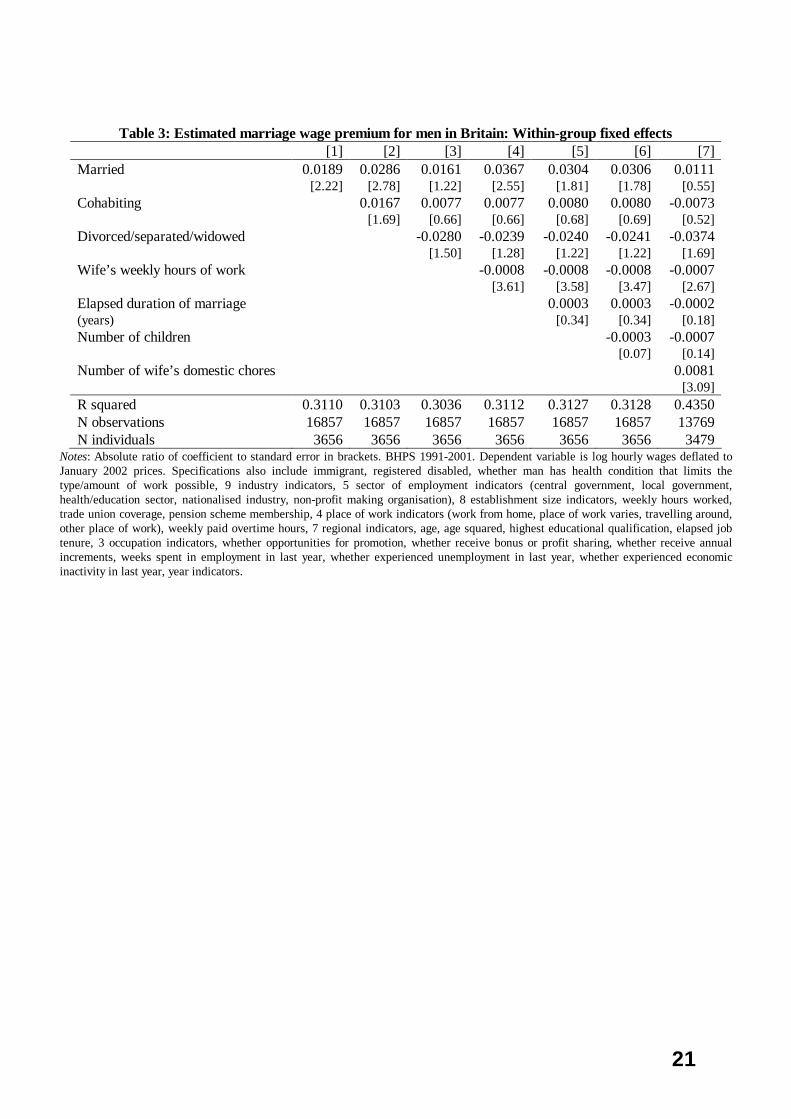
Fixed effects

Table 3 presents the estimates from the within-group fixed effects models.11 These estimates

indicate that, when allowing for time invariant unobserved characteristics, the size of the

marriage premium falls dramatically to between 1% and 4%. This suggests that a large

proportion of the premium observed in the OLS estimates is due to unobserved characteristics

that are positively correlated with both marriage and wages, consistent with the selection and

signalling arguments. However, in five of the seven specifications marriage still has a positive

impact on wages that at least borders on statistical significance, and that can be attributed to

productivity effects. Of the other variables of interest in these specifications, only the wife’s

weekly hours of work remain statistically significant. Each additional hour worked by the wife

reduces the wage premium by 0.08%, suggesting that a married man whose wife works a 40

hour week enjoys no wage premium relative to a single never married man, compared to a

11 There were 338 marriage formations and 105 marriage dissolutions within our sample over the period.

13

premium of 3% for a married man whose wife does not work (calculated on the basis of

specification [6]). The fact that cohabitation has no effect on wages is evidence against both

the specialisation and human capital accumulation hypotheses. The loss of the premium on

marital dissolution is evidence against the human capital accumulation hypothesis in favour of

specialisation. The negative impact of wife’s working hours supports both the human capital

accumulation and specialisation hypotheses, while the insignificance of marriage duration

supports employer discrimination over human capital accumulation.

In specification [7], where the direct measures of the degree of household specialisation are

entered, the marriage premium disappears – the coefficient, although positive, is no longer

statistically significant. However, the coefficient on the household specialisation variable is

positive and statistically significant, indicating that each additional domestic chore carried out

by the spouse increases the man’s wages by 0.8%. A married man whose wife is responsible

for all four domestic chores receives a wage premium of 3.2% relative to a single never

married man, although this premium is lost if the wife also works 40 hours per week in the

labour market. These results suggest that a large proportion of the marriage premium

observed in cross-sectional analysis is due to unobserved characteristics correlated with both

marriage and wages. Any remaining premium, attributable to higher productivity, can be

explained by specialisation within the household.

Random effects

Table 4 presents the estimates from the random effects specifications. These estimates show

that marriage is associated with a wage premium of between 2.5% (specification [1] and [7])

and 5.8% (specification [4]), which lie between the OLS and the fixed effects estimates.

Cohabiting men enjoy a wage premium over single never married men of about 2% (which

borders on statistical significance) while each additional hour worked by the wife reduces the

premium by 0.08%. Marriage duration, the number of children and previously being married

have no effect on wages. As in the fixed effects specifications, the marriage premium is no

longer statistically significant once the number of household chores for which the spouse is

responsible is entered (specification [7]), while each chore carried out by the spouse increases

the man’s wages by 0.8%. Again, these results favour the signalling and specialisation

hypotheses over the human capital accumulation hypothesis.

14

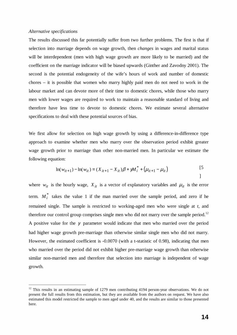
Alternative specifications

The results discussed this far potentially suffer from two further problems. The first is that if

selection into marriage depends on wage growth, then changes in wages and marital status

will be interdependent (men with high wage growth are more likely to be married) and the

coefficient on the marriage indicator will be biased upwards (Ginther and Zavodny 2001). The

second is the potential endogeneity of the wife’s hours of work and number of domestic

chores – it is possible that women who marry highly paid men do not need to work in the

labour market and can devote more of their time to domestic chores, while those who marry

men with lower wages are required to work to maintain a reasonable standard of living and

therefore have less time to devote to domestic chores. We estimate several alternative

specifications to deal with these potential sources of bias.

We first allow for selection on high wage growth by using a difference-in-difference type

approach to examine whether men who marry over the observation period exhibit greater

wage growth prior to marriage than other non-married men. In particular we estimate the

following equation:

( )ititiitititit MXXww µµγβ −++−=− +++ 1*

11 )()ln()ln( [5

]

where itw is the hourly wage, itX is a vector of explanatory variables and itµ is the error

term. *iM takes the value 1 if the man married over the sample period, and zero if he

remained single. The sample is restricted to working-aged men who were single at t, and

therefore our control group comprises single men who did not marry over the sample period.12

A positive value for the γ parameter would indicate that men who married over the period

had higher wage growth pre-marriage than otherwise similar single men who did not marry.

However, the estimated coefficient is -0.0070 (with a t-statistic of 0.98), indicating that men

who married over the period did not exhibit higher pre-marriage wage growth than otherwise

similar non-married men and therefore that selection into marriage is independent of wage

growth.

12 This results in an estimating sample of 1279 men contributing 4194 person-year observations. We do not present the full results from this estimation, but they are available from the authors on request. We have also estimated this model restricted the sample to men aged under 40, and the results are similar to those presented here.

15

The second way we allow for selection on high wage growth is through instrumental variables

(IV). We use a man’s responses to a set of attitudinal questions as instruments for being

married – they are assumed to influence the probability of being married but not wages

conditional on marriage. Individuals are asked the extent to which they personally agree or

disagree with the following statements:

- A preschool child is likely to suffer if his/her mother works; - All in all, family life suffers when the woman has a full-time job; - A woman and her family would all be happier if she goes out to work; - Both the husband and wife should contribute to the household income; - Having a full-time job is the best way for a woman to be an individual person; - A husband’s job is to earn money; a wife’s job is to look after the home and family; - Children need a father to be as closely involved in their upbringing as the mother; - Employers should make special arrangements to help mothers combine jobs and childcare; - A single parent can bring up children as well as a couple.

We create 9 binary variables that take the value 1 if a man agrees or strongly agrees with the

statement in question, and zero otherwise, and use these as instruments for being married.13

We interpret a man’s responses to these questions as signals of his attractiveness in the

marriage market. Following Bound et al (1995) and Staiger and Stock (1997), we check for

the validity of the instruments in two ways. Firstly, any potential instruments should

significantly improve the first-stage model determining the endogenous variable (in our case

the probability of being married). The results from likelihood ratio tests indicate that the

inclusion of these attitudinal variables leads to a significant improvement in the explanatory

power of the marriage probit at the 0.1% level of significance (χ2(9)=283.7). The second

indicator suggested by Bound et al (1995) is the increase in the adjusted R2. The model

explains almost 2% more of the total variation when the instruments are added to the marriage

probit.14

The estimates presented in the first panel of Table 5 result from pooled OLS, pooled IV, fixed

effects IV and random effects IV respectively. The estimated coefficients on the married

variable in the IV specifications are large, positive and (with the exception of the fixed effects

13 Note that the sample sizes are lower in these IV estimates. This is because of missing information in men’s responses to the attitude questions. 14 As our first-stage equation is a probit model, the R2s refer to pseudo-R2s. The validity of these variables as instruments for marriage is reinforced by the fact that they prove to be both independently and jointly insignificant when entered into a wage equation.

16

specification) statistically significant. It appears that selection based on wage growth did not

bias our previous estimates.

The estimates in the next panel of Table 5 deal with the potential endogeneity of the wife’s

working hours. We do this by creating 9 binary variables based on the wife’s responses to the

family attitude questions discussed previously and using these and also her age as instruments

for her working hours. This necessitates focusing on married men only, and we present OLS

estimates of wife’s working hours on married men’s wages as a comparison. Again, these

attitudinal questions prove to be valid instruments. A test for their joint significance in the

first-stage hours equation yields an F-statistic of 33.1, which is much higher than the values of

1 and 5 that Bound et al (1995) and Staiger and Stock (1997) suggest could signal weak

instruments. They generate a partial R2 of 0.02, which is ten times greater than the first-stage

partial R2 which generated concern for Bound et al (1995). The IV estimates are more

negative than those in the OLS specification, and are statistically significant, indicating that the

potential endogeneity of the wife’s work hours did not bias our earlier results.

The final panel in Table 5 deals with the potential endogeneity of the number of domestic

chores for which the wife is mostly responsible. Again we use the wife’s responses to the

family attitude questions discussed previously and her age as instruments, which again

necessitates focusing on married men only, and we present the comparable OLS estimates.

The responses to the attitudinal questions prove to be valid instruments – the results from

likelihood ratio tests indicate that the inclusion of the instruments leads to a significant

improvement at the 0.1% level of significance (χ2(11)=136.5) in the explanatory power of the

ordered probit modelling the number of chores for which the wife is mainly responsible. This

ordered probit model explains 1.3% more of the total variation when the instruments are

added.15 The IV estimates remain positive and statistically significant, indicating that the

potential endogeneity of the number of chores for which the wife is mainly responsible did not

bias our earlier results.

Conclusions

15 In this case, our first-stage equation is an ordered probit model, and the R2s refer to pseudo-R2s.

17

In this paper we provide new and unique evidence on the relationship between marriage and

wages among men in Britain. Cross-sectional analysis yields a wage premium for married men

of about 15%, consistent with much of the previous literature. Using panel data and panel data

methods, we find that this premium falls dramatically, indicating that about three-quarters of

the observed premium in cross-sectional analysis is caused by unobserved individual

heterogeneity and/or selection effects. Married men have unobserved characteristics that are

also correlated with wages. The proportion of the premium explained by unobserved

individual factors is similar to that found in the US literature. Korenman and Neumark (1991)

find less than half of the premium is accounted for by unobserved individual specific effects,

while Cornwell and Rupert (1995) find that the estimated returns to marriage are virtually zero

once such effects are allowed for. Our results are consistent with the hypothesis that

employers use marriage as a signal – a large proportion of the marriage premium is due to

unobservable characteristics that are valued both by wives and by employers, such as

motivation, loyalty, dependability and determination. Further research focussing on linked

worker-firm data may shed more light on this issue.

Nevertheless, a relatively small but statistically significant marriage premium remains even

when allowing for a wide range of individual, household, job and employer-related

characteristics and time invariant individual specific unobservable effects. Our preferred panel

estimates indicate the size of this premium increases with the number of domestic chores for

which the spouse is mostly responsible, and falls with the wife’s working hours. The relative

sizes of the coefficients suggest that a married man whose wife does not work but whose wife

is mostly responsible for four domestic chores enjoys a wage premium of about 4% relative to

a single never married man. However this premium almost disappears if the wife also works 40

hours per week in the labour market. We show that the effects of the hours worked and

domestic chores carried out by the wife are genuine, and not due to the potential endogeneity

of the wife’s decision to work. Our estimates therefore provide some evidence in favour of the

specialisation explanation for the enhanced productivity of married men.

References Becker, G.S. (1973), “A theory of marriage: Part I”, Journal of Political Economy, 81 (4),

pp.813-846. Becker, G.S. (1974), “A theory of marriage: Part II”, Journal of Political Economy, 82 (2),

pp.S11-S26. Becker, G.S. (1991), A treatise on the family, Cambridge MA: Havard University Press.

18

Blanchflower, D. and A.J. Oswald (2004), “Well being over time in Britain and the USA”, Journal of Public Economics, 88, pp.1359-1386.

Bound, J., D.A. Jaeger, R.M. Baker (1995), “Problems with instrumental variables estimation when the correlation between the instruments and the endogenous explanatory variable is weak”, Journal of the American Statistical Association, 90 (430), pp.443-450.

Chamberlain, G. (1984), Panel Data, in Z. Griliches and M.D. Intriligator (eds), Handbook of Econometrics Vol. 2, North Holland, Amsterdam.

Chun, H. and I. Lee (2001), “Why do married men earn more: Productivity or marriage selection?”, Economic Inquiry, 39 (2), pp.307-319.

Cornwell, C. and P. Rupert (1995), “Marriage and earnings”, Federal Reserve Bank of Cleveland Economic Review, 31 (4), pp.10-20.

Daniel, K. (1992), “Does marriage make men more productive?” NORC Discussion Paper no. 92-2, University of Chicago.

Davies, H. and R. Peronaci (1997), “Male wages and living arrangements: Recent evidence for Britain”, Discussion Paper in Economics, 5/97, Birkbeck college, University of London.

Diener, E., C.L. Gohm, E.M. Suh and S. Oishi (2000), “Subjective well being: Three decades of progress”, Psychological Bulletin, 125(2), pp.276-303.

Disney, R. and E. Whitehouse (1996), “What are occupational pension plan entitlements worth in Britain?”, Economica, 63, pp.213-38.

Ginther, D.K. and M. Zavodny (2001), “Is the male marriage premium due to selection? The effect of shotgun weddings on the return to marriage”, Journal of Population Economics, 14, pp.313-328.

Gray, J.S. (1997), “The fall in men’s return to marriage: Declining productivity effects or changing selection?”, Journal of Human Resources, 32 (3), pp.481-504.

Greenhalgh, C. (1980), “Male-female wage differentials in Great Britain: Is marriage an equal opportunity?”, Economic Journal, 90, pp.751-775.

Grove, W.R. (1973), “Sex, marital status and mortality”, American Journal of Sociology, 79 (1), pp.45-67.

Jacobsen, J. and W. Rayack (1996), “Do men whose wives work really earn less?”, American Economic Review, 86 (2), pp.268-273.

Joshi, H. and M-L Newell (1989), Pay differentials and parenthood: Analysis of men and women born in 1946, Research Report, Institute for Employment Research, University of Warwick.

Korenman, S. and D. Neumark (1991), “Does marriage really make men more productive?”, Journal of Human Resources, 26(2), pp.282-307.

Loh, E.S (1996), “Productivity differences and the marriage wage premium for white males”, Journal of Human Resources, 31 (3), pp.566-589.

Myers, D.G. (1999), “Close relationship and quality of life”, in D. Kahneman, E. Diener and N. Schwarz (eds) Well-being: The foundations of hedonic psychology, New York: Russell Sage Foundation.

Nakosteen, R.A. and M.A. Zimmer (1987), “Marital status and the earnings of young men: A model with endogenous selection”, Journal of Human Resources, 22 (2), pp.248-268.

Reed, R. and K. Hartford (1989), “The marriage wage premium and compensating wage differentials”, Journal of Population Economics, 2, pp.237-265.

Ribar, D. (2004), “What do social scientists know about the benefits of marriage? A review of quantitative methodologies”, IZA Discussion paper no. 998.

Ross, C.E., J. Mirowsky and K. Goldsteen (1990), “The impact of family on health: The decade in review”, Journal of Marriage and the Family, 52 (4), pp.1059-1078.

19

Schoeni, R.F. (1995), “Marital status and earnings in developed countries”, Journal of Population Economics, 8, pp.351-359.

Staiger, D. and J.H. Stock (1997), “Instrumental variables regression with weak instruments”, Econometrica, 65 (3), pp.557-586.

Stratton, L. (2002), “Examining the wage differential for married and cohabiting men”, Economic Inquiry, 40 (2), pp.199-212.

Stutzer, A. and B.S. Frey (2003), “Does marriage make people happy, or do happy people get married?”, Institute for Empirical Research in Economics, University of Zurich, working paper 143.

Waite, L.J. and M. Gallagher (2000), The case for marriage: Why married people are happier, healthier and better off financially, New York: Doubleday.

Wilson C.M. and A.J. Oswald (2002), “How does marriage affect physical and psychological health? A survey of the longitudinal evidence”, unpublished manuscript, University of Warwick.

20

Table 1: Average hourly wages by marital status for men Marital status Mean wage Standard deviation N person-years Single never married 7.53 4.80 3355 Married 10.80 6.94 10303 Cohabiting 9.04 6.36 2368 Divorced/separated/widowed 9.90 5.94 829 Total 9.85 6.57 16857 BHPS 1991-2001. Hourly wages deflated to January 2002 prices.

Table 2: Estimated marriage wage premium for men in Britain: OLS [1] [2] [3] [4] [5] [6] [7] Married 0.0917 0.1212 0.1433 0.1776 0.1611 0.1303 0.0912 [7.67] [8.60] [8.99] [9.58] [7.09] [5.36] [3.40] Cohabiting 0.0733 0.0904 0.0906 0.0908 0.0844 0.0511 [5.12] [5.86] [5.88] [5.90] [5.45] [2.92] Divorced/separated/widowed 0.0745 0.0758 0.0798 0.0784 0.0798 [2.74] [2.79] [2.90] [2.86] [2.74] Wife’s weekly hours of work -0.0016 -0.0016 -0.0012 -0.0011 [4.13] [4.11] [3.06] [2.59] Elapsed duration of marriage 0.0012 0.0015 0.0006 (years) [1.16] [1.45] [0.58] Number of children 0.0177 0.0135 [2.92] [2.11] Number of wife’s domestic chores 0.0189 [4.72] R squared 0.5953 0.5968 0.5975 0.5987 0.5988 0.5994 0.6019 N observations 16857 16857 16857 16857 16857 16857 13769 N individuals 3656 3656 3656 3656 3656 3656 3479

Notes: Absolute ratio of coefficient to standard error in brackets. BHPS 1991-2001. Dependent variable is log hourly wages deflated to January 2002 prices. Specifications also include immigrant, registered disabled, whether man has health condition that limits the type/amount of work possible, 9 industry indicators, 5 sector of employment indicators (central government, local government, health/education sector, nationalised industry, non-profit making organisation), 8 establishment size indicators, weekly hours worked, trade union coverage, pension scheme membership, 4 place of work indicators (work from home, place of work varies, travelling around, other place of work), weekly paid overtime hours, 7 regional indicators, age, age squared, highest educational qualification, elapsed job tenure, 3 occupation indicators, whether opportunities for promotion, whether receive bonus or profit sharing, whether receive annual increments, weeks spent in employment in last year, whether experienced unemployment in last year, whether experienced economic inactivity in last year, year indicators.

21

Table 3: Estimated marriage wage premium for men in Britain: Within-group fixed effects [1] [2] [3] [4] [5] [6] [7] Married 0.0189 0.0286 0.0161 0.0367 0.0304 0.0306 0.0111 [2.22] [2.78] [1.22] [2.55] [1.81] [1.78] [0.55] Cohabiting 0.0167 0.0077 0.0077 0.0080 0.0080 -0.0073 [1.69] [0.66] [0.66] [0.68] [0.69] [0.52] Divorced/separated/widowed -0.0280 -0.0239 -0.0240 -0.0241 -0.0374 [1.50] [1.28] [1.22] [1.22] [1.69] Wife’s weekly hours of work -0.0008 -0.0008 -0.0008 -0.0007 [3.61] [3.58] [3.47] [2.67] Elapsed duration of marriage 0.0003 0.0003 -0.0002 (years) [0.34] [0.34] [0.18] Number of children -0.0003 -0.0007 [0.07] [0.14] Number of wife’s domestic chores 0.0081 [3.09] R squared 0.3110 0.3103 0.3036 0.3112 0.3127 0.3128 0.4350 N observations 16857 16857 16857 16857 16857 16857 13769 N individuals 3656 3656 3656 3656 3656 3656 3479

Notes: Absolute ratio of coefficient to standard error in brackets. BHPS 1991-2001. Dependent variable is log hourly wages deflated to January 2002 prices. Specifications also include immigrant, registered disabled, whether man has health condition that limits the type/amount of work possible, 9 industry indicators, 5 sector of employment indicators (central government, local government, health/education sector, nationalised industry, non-profit making organisation), 8 establishment size indicators, weekly hours worked, trade union coverage, pension scheme membership, 4 place of work indicators (work from home, place of work varies, travelling around, other place of work), weekly paid overtime hours, 7 regional indicators, age, age squared, highest educational qualification, elapsed job tenure, 3 occupation indicators, whether opportunities for promotion, whether receive bonus or profit sharing, whether receive annual increments, weeks spent in employment in last year, whether experienced unemployment in last year, whether experienced economic inactivity in last year, year indicators.

22

Table 4: Estimated marriage wage premium for men in Britain: Random effects [1] [2] [3] [4] [5] [6] [7] Married 0.0258 0.0392 0.0359 0.0583 0.0449 0.0419 0.0253 [3.05] [3.85] [2.76] [4.11] [2.69] [2.45] [1.26] Cohabiting 0.0223 0.0198 0.02158 0.0218 0.0211 0.0082 [2.25] [1.72] [1.88] [1.89] [1.82] [0.59] Divorced/separated/widowed -0.0079 -0.0015 -0.0005 0.0006 -0.0057 [0.43] [0.08] [0.03] [0.03] [0.26] Wife’s weekly hours of work -0.0008 -0.0008 -0.0008 -0.0007 [3.69] [3.62] [3.25] [2.48] Elapsed duration of marriage 0.0010 0.0010 0.0007 (years) [1.01] [1.00] [0.65] Number of children 0.0039 0.0039 [0.93] [0.82] Number of wife’s domestic chores 0.0083 [3.18] R squared 0.6137 0.6147 0.6147 0.6167 0.6166 0.6169 0.6208 N observations 16857 16857 16857 16857 16857 16857 13769 N individuals 3656 3656 3656 3656 3656 3656 3479

Notes: Absolute ratio of coefficient to standard error in brackets. BHPS 1991-2001. Dependent variable is log hourly wages deflated to January 2002 prices. Specifications also include immigrant, registered disabled, whether man has health condition that limits the type/amount of work possible, 9 industry indicators, 5 sector of employment indicators (central government, local government, health/education sector, nationalised industry, non-profit making organisation), 8 establishment size indicators, weekly hours worked, trade union coverage, pension scheme membership, 4 place of work indicators (work from home, place of work varies, travelling around, other place of work), weekly paid overtime hours, 7 regional indicators, age, age squared, highest educational qualification, elapsed job tenure, 3 occupation indicators, whether opportunities for promotion, whether receive bonus or profit sharing, whether receive annual increments, weeks spent in employment in last year, whether experienced unemployment in last year, whether experienced economic inactivity in last year, year indicators, individual means of the time-varying covariates, see text for details.

23

Table 5: Alternative specifications All men OLS IV Fixed

effects IV Random

effects IV Married 0.0896 0.3598 0.1543 0.2806 [7.35] [4.40] [1.04] [2.50] R squared 0.5929 0.5483 0.3765 0.5820 N observations 16148 16148 16148 16148 N individuals 3339 3339 3339 3339 Married men only OLS IV Fixed

effects IV Random

effects IV Wife’s weekly -0.0016 -0.0037 -0.0021 -0.0029 hours of work [4.31] [4.55] [2.83] [4.90]

R squared 0.5722 0.5687 0.1872 0.6011 N observations 10182 10182 10182 10182 N individuals 2096 2096 2096 2096 OLS IV Fixed

effects IV Random

effects IV Number of wife’s domestic chores 0.0194 0.1010 0.0387 0.0563 [4.26] [7.63] [2.54] [4.24] R squared 0.5784 0.5738 0.3006 0.6058 N observations 8207 8207 8207 8207 N individuals 2010 2010 2010 2010

Notes: Absolute ratio of coefficient to standard error in brackets. BHPS 1991-2001. Dependent variable is log hourly wages deflated to January 2002 prices. Specifications also include immigrant, registered disabled, whether man has health condition that limits the type/amount of work possible, 9 industry indicators, 5 sector of employment indicators (central government, local government, health/education sector, nationalised industry, non-profit making organisation), 8 establishment size indicators, weekly hours worked, trade union coverage, pension scheme membership, 4 place of work indicators (work from home, place of work varies, travelling around, other place of work), weekly paid overtime hours, 7 regional indicators, age, age squared, highest educational qualification, elapsed job tenure, 3 occupation indicators, whether opportunities for promotion, whether receive bonus or profit sharing, whether receive annual increments, weeks spent in employment in last year, whether experienced unemployment in last year, whether experienced economic inactivity in last year, year indicators. Random effects estimation in addition includes individual means of the time-varying covariates, see text for details. Man’s family attitude questions used as instruments for Married. Wife’s family attitude questions and age used as instruments for wife’s working hours and number of wife’s domestic chores.