The DLR Ground Station in the Optical Payload Experiment (STROPEX) - Results of the Atmospheric Measurement Instruments

Markus Knapek*a, Joachim Horwatha, Nicolas Perlota, Brandon Wilkersonb

aGerman Aerospace Center, Institute for Communications and Navigation bU.S. Air Force Exchange Engineer

ABSTRACT

Optical communication at 1.25Gbps was successfully demonstrated in a downlink from a stratospheric balloon platform at 22km altitude to a Transportable Optical Ground Station. The experiments took place at ESRANGE, Kiruna, Sweden in August 2005. In addition to optical communications, several atmospheric measurement instruments (Differential Image Motion Monitor, Turbulence Profiler) were used to study the influence of atmospheric turbulence on the optical link. A description of the measurement instruments is given and results of the turbulence instruments (Fried parameter r0, Cn

2 profile) are presented.

Keywords: Optical Free-Space Communications, Stratospheric Platform, High Altitude Platform, CAPANINA

1. INTRODUCTION

Laser free-space communication technologies in space and aeronautical applications show some major advantages over RF and microwave technologies. Laser communication allows higher data rates with lower power consumption requirements, weight, and size. Disadvantages of optical communications like clouds can be countered with various mitigation schemes like ground station diversity [1].

This paper will give a short overview of the balloon experiments and the technical design of the optical ground station, however it will concentrate mainly on the background of the measurement instruments and the results describing the atmospheric turbulence conditions along the path.

The Optical Communications Group within the Institute of Communications and Navigation at DLR has developed a Transportable Optical Ground Station (TOGS) for the deployment in various application scenarios and at different locations. For the described balloon experiment the TOGS was built up on the balloon launch pad of ESRANGE. The TOGS was covered during setup by a movable tent to protect the sensitive equipment and to allow the preparation of all instruments. Shortly before the experiment the tent was removed.

The launch took place at 3:45 a.m. local time (UTC+2h) and the balloon ascended to the target altitude of 22km at around 5:00 a.m. Details on the flight system including the flight trajectory can be found in [2]. Results of the atmospheric measurements will be presented in Section 4. Fig. 1 shows the first test of the TOGS with a tethered balloon in the UK 2004. For this test a small telescope with only 20cm aperture was used. Fig. 2 shows the TOGS at the test site in Kiruna. The measurement instruments are located under the black cover.

*Markus Knapek is with the German Aerospace Center DLR, Institute for Communications and Navigation, Oberpfaffenhofen, 82234 Wessling, Germany (phone: ++49-8153-282879; fax: ++49-8153-282844; e-mail: Markus.Knapek@dlr.de).

Copyright 2006 Society of Photo-Optical Instrumentation Engineers. This paper was published in Proceedings of the SPIE Vol. 6304 and is made

available as an electronic reprint with permission of SPIE. One print or electronic copy may be made for personal use only. Systematic or multiple reproduction, distribution to multiple locations via electronic or other means, duplication of any material in this paper for a fee or for commercial purposes, or modification of the content of the paper are prohibited.

2. TECHNICAL OVERVIEW OF THE TRANSPORTABLE OPTICAL GROUND STATION The central component of the TOGS is a 40cm Cassegrain telescope. A telescope of this size has sufficient aperture to perform optical communications with geostationary satellites and is still small enough to keep the structure transportable and low-cost. A commercially available astronomical mount is used to point the telescope at the targets in the different scenarios.

The flight terminal sent the communication beam on a wavelength of 1550nm. 1550nm is not detectable by the standard silicon cameras, which are deployed for the atmospheric measurement instruments. Therefore a second co-aligned beam at 986nm was used for the measurement instruments. The TOGS used beacon lasers at 810nm to illuminate the flight terminal and thus enable acquisition.

Fig. 3 shows the system components of the optical ground station. Three main parts can be identified. The mount control system on the left includes the mount calibration and open-loop pointing capabilities for satellite tracking and GPS target tracking. The visual pointing, tracking, and acquisition (PAT) system with a wide field-of-view (FOV) and a narrow FOV camera is displayed in the middle. The measurement systems on the right include the Turbulence Profiler (TP), the Differential Image Motion Monitor (DIMM), and a power sensor. A RAID hard disk array with 8 disks is connected to the measurement instruments to handle the large amount of image material. All components are connected by TCP/IP, which allows clock synchronization of all computers via Network Time Protocol (NTP).

For the balloon experiments in August 2005 the GPS position of the balloon was sent to the ground station via radio link, and the TOGS could calculate the pointing angle based on its own position/orientation and the target’s GPS position. The acquisition of the target is a two-step process. First, the telescope is pointed at the target open-loop, i.e. without visual feed-back. The system is designed to be accurate enough to get the target into the camera's FOV. Next, the target is acquired on the acquisition (wide FOV) and tracking camera (narrow FOV), and the closed-loop tracking keeps the target centered in the FOV with high accuracy (<50µrad), so that an uninterrupted communication is ensured.

A central part of the TOGS is the Atmospheric Turbulence Monitor (ATM), which combines several optical measurement instruments to characterize the atmospheric turbulence on the optical link. In this way, the ATM helps to understand the influences of the atmosphere on the optical link during various atmospheric conditions.

The ATM measurements are used to reconstruct the atmospheric parameters along the path of the optical link. These parameters help to analyze the performance of the communication system. They also can be used for simulation tools like the DLR developed PiLab [3]-[5].

Fig. 1 In 2004 the Transportable Optical Ground Station in a downlink from a tethered balloon in the UK.

Fig. 2 The Transportable Optical Ground Station during the balloon trial in Kiruna, Sweden, August 2005.

3. ATMOSPHERIC TURBULENCE MONITOR

The Atmospheric Turbulence Monitor (ATM) consists of three instruments to measure atmospheric turbulence on the path of the optical link:

− The Differential Image Motion Monitor (DIMM) measures the Fried parameter r0, which is a measure of the wavefront distortion or coherence length under atmospheric conditions.

− The Turbulence Profiler (TP) allows the reconstruction of the Cn2 profile along the path of the transmission and

gives a measure of the scintillation index. − A power sensor. The DIMM and the TP are implemented with cameras, which guarantee flexibility for various application scenarios and a good resolution. For the TP a QImaging QICAM-IR (696x520 pixels, 12bits) and for the DIMM a Basler A602f (CMOS, 656 x 491 pixels, 8bits) are used.

Fig. 4 shows the principle optical design of the ATM in a Zemax simulation. The beam from the Cassegrain telescope is collimated and split up by beam splitter cubes to the measurement instruments and the tracking camera.

Fig. 3 System components of the optical ground station: mount control system, closed-loop visual tracking system, and Atmospheric Transmission Monitor (Turbulence Profiler, DIMM, Power Sensor).

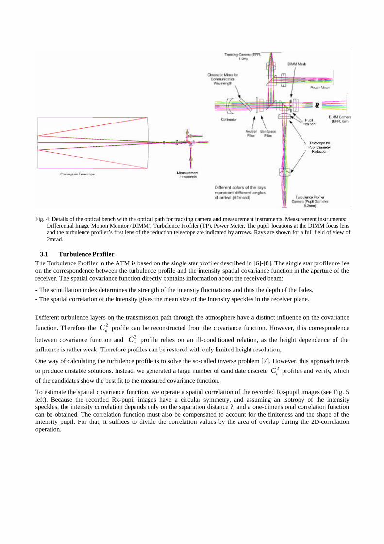
3.1 Turbulence Profiler The Turbulence Profiler in the ATM is based on the single star profiler described in [6]-[8]. The single star profiler relies on the correspondence between the turbulence profile and the intensity spatial covariance function in the aperture of the receiver. The spatial covariance function directly contains information about the received beam:

- The scintillation index determines the strength of the intensity fluctuations and thus the depth of the fades. - The spatial correlation of the intensity gives the mean size of the intensity speckles in the receiver plane. Different turbulence layers on the transmission path through the atmosphere have a distinct influence on the covariance

function. Therefore the 2nC profile can be reconstructed from the covariance function. However, this correspondence

between covariance function and 2nC profile relies on an ill-conditioned relation, as the height dependence of the

influence is rather weak. Therefore profiles can be restored with only limited height resolution.

One way of calculating the turbulence profile is to solve the so-called inverse problem [7]. However, this approach tends

to produce unstable solutions. Instead, we generated a large number of candidate discrete 2nC profiles and verify, which

of the candidates show the best fit to the measured covariance function.

To estimate the spatial covariance function, we operate a spatial correlation of the recorded Rx-pupil images (see Fig. 5 left). Because the recorded Rx-pupil images have a circular symmetry, and assuming an isotropy of the intensity speckles, the intensity correlation depends only on the separation distance ?, and a one-dimensional correlation function can be obtained. The correlation function must also be compensated to account for the finiteness and the shape of the intensity pupil. For that, it suffices to divide the correlation values by the area of overlap during the 2D-correlation operation.

Fig. 4: Details of the optical bench with the optical path for tracking camera and measurement instruments. Measurement instruments: Differential Image Motion Monitor (DIMM), Turbulence Profiler (TP), Power Meter. The pupil locations at the DIMM focus lens and the turbulence profiler’s first lens of the reduction telescope are indicated by arrows. Rays are shown for a full field of view of 2mrad.

The covariance function is readily obtained from the correlation function by subtracting the square of the mean intensity. Finally, because the fluctuations are independent of the mean optical intensity, the covariance function is divided by the square of the mean intensity.

The profile restoration procedure can be decomposed as follows:

1) Choice of an expected standard profile as initial profile. The atmospheric path is divided into turbulence layers. For each turbulence layer, standard Cn

2 values covering several orders of magnitude are chosen.

2) Calculation of the covariance function corresponding to the candidate turbulence profile. From scintillation theory, we know that, under weak fluctuations, the covariance function ( )B ρ is related to the profile 2 ( )nC z by means of weighting

functions ( , )W z ρ (e.g. [6])

( ) 2

0

( ) ( , )L

nB C z W z dzρ ρ= ∫ , (1)

where z is the distance from the receiver. The weighting functions depend on the type of propagated wave. Our candidate Cn

2 profiles are discrete profiles. The covariance function ˆ( )B ρ corresponding to each discrete candidate Cn2 profile is

calculated according to

( ) ( )2

1

ˆ ( ) ,N

i n i ii

B z C z W zρ ρ=

= ∆ ⋅ ⋅∑ (2)

3) Selection of the best candidate profiles. All the candidate profiles are tested and sorted according to the mean-square (MS) of the covariance deviation:

2

00ˆ( ) ( )MS B B dρ ρ ρ

∞ = − ∫ (3)

where B0 is the measured covariance function. Several iterations of the procedure are applied until the deviation from the measured covariance function becomes sufficiently small.

Equation (2) represents a linear system. However, a linear restoration of the 2nC values does not take into account that

the 2nC values have to be positive. A formulation with 2 2

ny C= ensures positive values of 2nC , however, it makes the

problem non-linear. Since the problem is not well-conditioned, non-linear solving methods already need good starting values to produce useful results. For the presented measurements good candidate profiles were produced by the above stated method. The best candidate then was further improved by a non-linear solver.

Fig. 5 Example of gathered turbulence data. Recorded turbulence profiler pupil intensity snapshot of the 40 cm Cassegrain telescope aperture with central obscuration (left). Recorded DIMM sample picture, with the two focal spots moving against each other (right).

For a plane wave, the weighting functions are given by [9]

2

2 2 8 / 30

0

( , ) 0.033 8 ( ) 1 cospl

zW z k J d

kκ

ρ π κ κρ κ∞

− = ⋅ −

∫ (4)

where k = λ/2π and J0 is the Bessel function of the first kind. For a spherical wave, the weighting functions are given by [9]

2

2 2 8/30

0

( , ) 0.033 8 1 1 cos 1sphz z zW z k J dL k L

κρ π κ κρ κ∞

− = ⋅ ⋅ − ⋅ − − ∫ (5)

3.2 Differential Image Motion Monitor The Differential Image Motion Monitor (DIMM) measures the angle-of-arrival of the incoming wave in two small apertures separated by a distance d (see Fig. 6). The waves from the two apertures are focussed by a lens, and one of the paths is transmitted through an optical wedge to generate two separate spots on a CCD camera. A rule for the dimensioning of the sub-aperture size Dsub and the inter-aperture distance d is given by

0subD r d< < , (6)

so that the angle-of-arrival does not change too much over the sub-aperture but enough between the two apertures [10]. Because the DIMM measures the differential spot motion, the technique is inherently insensitive to tracking errors. This characteristic is especially important for dynamic scenarios, where the ground station will always have residual tracking errors. An example for the two spots on the DIMM sensor can be seen in Fig. 5 (right image).

The calculation of the Fried parameter r0 from the differential variance of the spot motion can be found, for example, in [10]. The shape of the incoming wavefront is proportional to the wavefront phase error ( , )x yΦ

( , ) ( , )2

z x y x yλπ

= Φ (7)

Hence, the angle-of-arrival fluctuations in the x direction can then be expressed by

( , ) ( , ) ( , )2

x y z x y x yx x

λα

π∂ ∂

= − = − Φ∂ ∂

. (8)

The covariance of the angle-of-arrival fluctuations is given by

( , ) ( , ) ( , )B x y x yα ξ η α α ξ η= ⋅ + + (9)

With the covariance function of a derivative [11]

2

' ' 2

( )( ) xx

x xB

Bτ

ττ

∂= −

∂ (10)

and the phase structure function

[ ]( , ) 2 (0,0) ( , )D B Bξ η ξ ηΦ Φ Φ= − , (11)

the covariance function of the angle-of-arrival fluctuations can be written as

2 2

2 2( , ) ( , )8

B Dαλξ η ξ ηπ ξ Φ

∂=∂

. (12)

Using the Kolmogorov turbulence at the near-field approximation

5

3

0

( , ) 6.88r

Dr

ξ ηΦ

=

(13)

where 2 2r ξ η= + , we get the expression for the angle-of-arrival fluctuations

5

62

2 5/3 2 20 2( , ) 0.087B rα ξ η λ ξ η

ξ− ∂ = ⋅ ⋅ + ∂

(14)

The measurement system in the ATM gives us the differential variance s 2 of the spot positions in longitudinal (along the connection line of the two mask apertures) and in transversal direction. To calculate the Fried parameter from the measurements we write for the variance of the differential spot motion

[ ]2 22(0) ( ) (0) ( ) (0) ( )d d dα ασ α α α α− = − − − (15)

[ ]22 (0) 2 (0) ( ) 2 (0) ( )d B B dα α α= − = −

where we set ( ) ( ,0)B d B dα= for longitudinal and ( ) (0, )B d B dα= for the transversal direction. The covariance

function in the origin however is limited by aperture averaging and is given by the angle-of-arrival variance (e.g. [12])

Fig. 6 Outline of the DIMM design. A mask with the two sub-apertures is placed in the plane of the exit pupil of the telescope. The incoming beam is focused by a lens, and one of the two paths is transmitted through an optical wedge to separate the spots in the focal plane of the DIMM camera.

5 /3 1/3

0

(0) (0,0) 0.179B Br Dαλ λ = = ⋅

. (16)

With these results, we calculate the Fried parameter in longitudinal direction r0,l and in transversal direction r0,t:

3 / 5

2 1/3

0, 2,

l Subl

d l

K Dr

λσ

− =

(17)

3/5

2 1/3

0, 2,

t Subt

d t

K Dr

λσ

− =

Fig. 7. Atmospheric coherence length r0 between 6:00 and 11:00 a.m.

Fig. 8. Profiler weighting functions with respect to height. The functions were calculated from equation (5) for a spherical wave for a 1550nm source in the zenith.

Fig. 9. Intensity scintillation index and power scintillation index for the 40cm telescope.

Fig. 10. Measured aperture averaging factor between intensity

and power scintillation index for the 40cm telescope 2

2P

I

σσ

.

with

1/3

0.358 1 0.541lSub

dK

D

− = −

1/3

0.358 1 0.810tSub

dK

D

− = −

4. EVALUATION OF ATMOSPHERIC MEASUREMENTS The measurements during the balloon trial started at 6:13am (local time) and ended at 11:01am. During this period 35 synchronous measurements of DIMM and TP were performed.

The estimation of the r0 parameter from the DIMM over the daytime is shown in Fig. 7. An r0 peak of up to 16cm with the best atmospheric conditions can be seen at about 8:00 a.m. The second curve in Fig. 7 shows the ro values reconstructed from the Cn

2 profiles measured by the TP. These reconstructed values confirm the development of r0 and show the increase between 8 a.m. and 9 a.m., however the reconstruction from the TP most of the time overestimates r0.

Fig. 8 shows the weighting functions according to equation (5) (spherical wave) used for the reconstruction of the TP. The weighting functions W(h) decrease to zero for both ends of the optical link, which implies that instrument becomes less sensitive to the turbulence close to the transmitter and the receiver.

The atmospheric coherence length can be reconstructed from the 2nC values by [9]

( )3

55

32 20

0

2.1 1.46 ( ) 1 /L

nz

r k C z z L dz−

=

= ⋅ ⋅ ⋅ ⋅ −

∫ (18)

This implies that r0 is mainly influenced by turbulence close to the receiver, since the 2nC value as well as the term

( )1 zL− decrease with z. The TP cannot estimate the 2

nC values close to the receiver, therefore the reconstructed r0

might become overestimated due to underestimated 2nC values near the receiver, where they have the strongest impact

on the r0. This might explain the difference of the r0 values of DIMM and TP visible in Fig. 7.

Fig. 9 shows the intensity scintillation index calculated from single pixels and the power scintillation index over the telescope aperture of 40cm. Both the intensity scintillation index as well as the power scintillation index show a minimum around 8 a.m. This corroborates the decrease of atmospheric turbulence during this hour. The turbulence minimum occurs approximately 2.5 hours after sunrise. Fig. 11 shows the sun elevation angle for the experiment period. Sunrise is at 5:15 a.m. Shortly after sunrise the turbulence level drops to a minimum, since the air and the ground have the same temperature and less turbulence is created by energy transfer processes.

Fig. 10 shows the measured aperture averaging factor for the 40cm telescope. The averaging factor indicates a decrease of the signal fluctuation by over a factor 10 due to the aperture size.

Several reconstructed 2nC profiles can be seen in Fig. 12. The

2nC profiles can only be calculated for a small number of

heights due to the ill-conditioned inverse problem of 2nC

Fig. 11. Sun elevation angle on the trial day (30th August 2005). Sunrise is at 5:15 a.m. and sunset at 20:00 p.m local time.

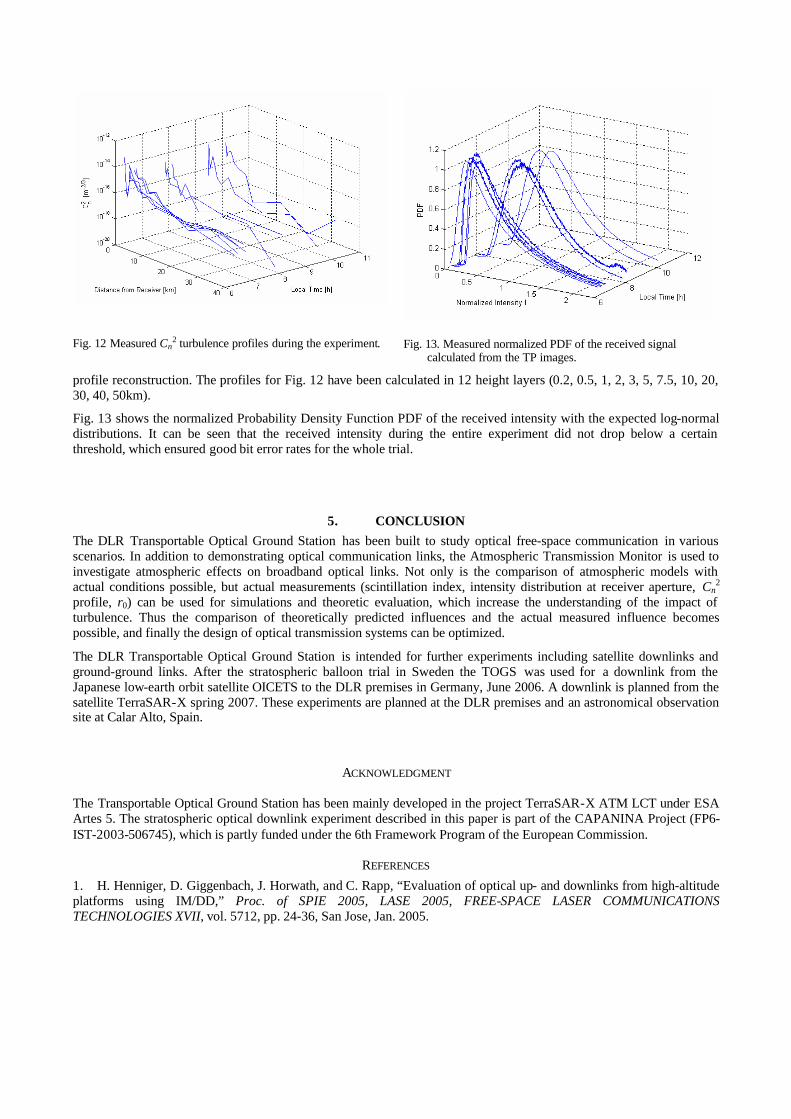
profile reconstruction. The profiles for Fig. 12 have been calculated in 12 height layers (0.2, 0.5, 1, 2, 3, 5, 7.5, 10, 20, 30, 40, 50km).

Fig. 13 shows the normalized Probability Density Function PDF of the received intensity with the expected log-normal distributions. It can be seen that the received intensity during the entire experiment did not drop below a certain threshold, which ensured good bit error rates for the whole trial.

5. CONCLUSION The DLR Transportable Optical Ground Station has been built to study optical free-space communication in various scenarios. In addition to demonstrating optical communication links, the Atmospheric Transmission Monitor is used to investigate atmospheric effects on broadband optical links. Not only is the comparison of atmospheric models with actual conditions possible, but actual measurements (scintillation index, intensity distribution at receiver aperture, Cn

2

profile, r0) can be used for simulations and theoretic evaluation, which increase the understanding of the impact of turbulence. Thus the comparison of theoretically predicted influences and the actual measured influence becomes possible, and finally the design of optical transmission systems can be optimized.

The DLR Transportable Optical Ground Station is intended for further experiments including satellite downlinks and ground-ground links. After the stratospheric balloon trial in Sweden the TOGS was used for a downlink from the Japanese low-earth orbit satellite OICETS to the DLR premises in Germany, June 2006. A downlink is planned from the satellite TerraSAR-X spring 2007. These experiments are planned at the DLR premises and an astronomical observation site at Calar Alto, Spain.

ACKNOWLEDGMENT

The Transportable Optical Ground Station has been mainly developed in the project TerraSAR-X ATM LCT under ESA Artes 5. The stratospheric optical downlink experiment described in this paper is part of the CAPANINA Project (FP6-IST-2003-506745), which is partly funded under the 6th Framework Program of the European Commission.

REFERENCES

1. H. Henniger, D. Giggenbach, J. Horwath, and C. Rapp, “Evaluation of optical up- and downlinks from high-altitude platforms using IM/DD,” Proc. of SPIE 2005, LASE 2005, FREE-SPACE LASER COMMUNICATIONS TECHNOLOGIES XVII, vol. 5712, pp. 24-36, San Jose, Jan. 2005.

Fig. 12 Measured Cn2 turbulence profiles during the experiment. Fig. 13. Measured normalized PDF of the received signal

calculated from the TP images.

2. J. Horwath, M. Knapek, B. Epple, M. Brechtelsbauer , and B. Wilkerson, “Broadband Backhaul Communication for Stratospheric Platforms: The Stratospheric Optical Payload Experiment (STROPEX),” Proceedings of the SPIE 2006, Free-Space Laser Communications VI, vol. 6304, San Diego, 2006. 3. J. Horwath, N. Perlot, D. Giggenbach, and R. Jüngling, "Numerical simulations of beam propagation through optical turbulence for high-altitude platform crosslinks", Proceedings of the SPIE 2004, vol. 5338B, 2004. 4. J. Horwath and N. Perlot, “Determination of statistical field parameters using numerical simulations of beam propagation through optical turbulence”, Proceedings of SPIE 2004, vol. 5338, 2004. 5. D. Giggenbach, F. David, R. Landrock, K. Pribil, E. Fischer, R. Buschner, and D. Blaschke, “Measurements at a 61 km near-ground optical transmission channel”, Free Space Laser Communication Technologies XIV, Proc. of SPIE 2002, vol. 4635, 2002. 6. A. Tokovinin and V. Kornilov, “Measuring turbulence profile from scintillations of single stars,” Astronomical Site Evaluation in the visible and Radio Range, Eds. Benkhaldoun Z., Muñoz-Tuñon C., Vernin J., ASP Conf. Ser., vol. 266, pp. 104-112, 2002. 7. A. Tokovinin, V. Kornilov, N. Shatsky, and O. Voziakova, “Restoration of turbulence profile from scintillation indices,” Mon. Not. R. Astron. Soc., vol. 343, no. 3, pp. 891-899, 2003. 8. J.L. Caccia, M. Azouit, and J. Vernin, “Wind and Cn

2 profiling by single-star scintillation analysis”, Appl. Opt., vol. 26, No 7, pp. 1288-1294, 1987. 9. L. C. Andrew and R. L. Phillips, Laser Beam Propagation through Random Media, SPIE Optical Engineering Press, Bellingham (WA), USA, 1998. 10. M. Sarazin and F. Roddier, “The ESO differential image motion monitor,” Astron. Astrophys., vol. 227, pp.294-300, 1990. 11. A. Papoulis, Probability, Random Variables, and Stochastic Processes, McGraw-Hill Series in Systems Science, 1965. 12. L. C. Andrew, R. L. Phillips, and C. Y. Hopen, Laser Beam Scintillation with Applications, SPIE Press, Bellingham (WA), USA, 2001.