49

Chapter 3

MARKOV PROCESS

50

Chapter 3MARKOV PROCESS

3.0 INTRODUCTION

Markov process is a stochastic or random process, that is used

in decision problems in which the probability of transition to any

future state depends on the current state and not on the manner in

which the specific state was reached.

Mathematically, nXP n122-n1n P{X}X,X,,X,X }X 1n

Markov analysis involves the studying of the present behavior of a

system to predict the future behavior of the same system. This is

introduced by Russian mathematician, Andrey A Markov. General

theory concerning Markov process was developed by A N Kolmogorov,

W.Feller and others. Markov processes are a certain special class of

mathematical models that are used in decision problems associated

with dynamic systems. Markov processes are widely used, perhaps, as

marketing aid for examining and predicting the customer behavior

concerning their loyalty to one brand of a given product and their

switching patterns to other brands of the same product. Other

applications that have been found for Markov processes include:

Manpower planning

Monsoon rainfall prediction

Forecast of wind power generation

Assessing the behaviour of stock prices

Scheduling hospital admissions

51

A simple Markov chain is a discrete random process with

Markovian property. In general the term Markov Chain is used to refer

a Markov Process that is discrete with finite state space. Usually a

Markov Chain would be defined for a discrete set of times (i.e. a

discrete-time Markov chain) although some authors use the same

terminology where time can take continuous values.

In a Markov process the possible states i.e. state space that a

system under focus could take at any point of time will be clearly

defined. As the system changes its state randomly it will be difficult to

predict the next future state with certainty. In this context the

statistical properties of the system for future state will be forecasted.

The change of system from one state to other state is called

Transition and the probability associated with this state transition is

called Transition Probability. The state space and the associated

transition probabilities characterize the Markov Chain.

For instance, the system may be a customer interested in a

certain commodity and have an option of selecting the commodity

from the available three brands namely – A, B and C. If the customer

selects the brand A, we might say that the system is in state 1. If the

customer selects the brand B, we might say that the system is in state

2 and if he/she selects the brand C, we might say that the system is

in state 3. Similarly the system might be inventory level of a given item

and a zero inventory could be denoted by state 1, one to ten units of

inventory could be denoted by state 2 and so on. Now the relevant

questions one may pose may be:

52

1. If the system is in state ‘i’ (i = 1,2,3…) say on day one, then what

is the probability that it is instate ‘j’ (j= 1,2,3…) in ‘n’ steps i.e. on

day 2 or day 3 or day 4 or … on day n?

2. After a larger number of steps (n ), what is the probability

that the system will be in state ‘s’?

3. If a company currently has a certain share of the market, what

share of the market will it have n steps from now?

Markov processes are capable of answering these and many other

questions relative to dynamic systems.

A simple Markov process is illustrated in the following example.

Let us consider monsoon rainfall over a particular region as a

system with two states – one as rainfall occurs and second as rainfall

does not occur. During monsoon, if rainfall occurs today, the

probability that there will be rainfall a day later is 0.7, and the

probability that there will be no rainfall a day later is 0.3. If there is no

rain fall today, the probability that there will be rainfall a day later is

0.6 and the probability that there will be no rainfall a day later is 0.4.

Let state-1 represents the rainfall and state-2 represents no rainfall

then the transition probabilities can be represented as given in the

Table 3.1.

Rain fall(State-1)

No rain fall(State-1)

Rain fall(State-1) 0.7 0.3

No rain fall(State-1) 0.6 0.4

Table 3.1: Transition probabilities for Monsoon rainfall example

53

The process is represented in Fig.3.1 by two flow diagrams whose

upward branches represent moving to state-1 and downward

branches represent moving to state-2.

Suppose the monsoon starts with state-1 (rainfall), there is a 0.7

probability that there will be rainfall on the 2nd day. Now consider

the state on 3rd day. The probability for state-1 on 3rd day is 0.67

(i.e. 0.49 + 0.18).

The corresponding probability that there will be state-2 in 3rd day,

given that it started in state-1 on 1st day, is 0.33 (i.e. 0.21 + 0.12).

Transition probabilities for next days can be computed in similar

manner.

Fig 3.1: Flow diagram representing the Markov Process

1

2

12

1

2

1

0.70.3

0.7

0.3

0.4

0.6

0.21

0.49

0.18

0.12

StartingwithState-1

1st day 2nd day 3rd day Transition probabilityon 3rd day

2

2

12

1

2

1

0.60.3

0.7

0.4

0.4

0.6

0.18

0.42

0.24

0.16

StartingwithState-2

1st day 2nd day 3rd day Transition probabilityon 3rd day

54

The Table 3.2 shows that the probability for the state-1 on any

future day tends towards 2/3, irrespective of the initial state on day-1.

This probability is called as Steady state probability of being in state-

1. On the similar lines, the steady state probability for the state-2 on

any future day is 1/3 (i.e. 1- 2/3).

DayNumber

Probability that there will be state-1 on a future day,given that it started in

STATE-1 on day-1 STATE-2 on day-1

1 1.0 0.02 0.7 0.63 0.67 … (2/3) 0.66 … (2/3)4 0.667 … (2/3) 0.666 … (2/3)5 0.6667 … (2/3) 0.6666 … (2/3)6 0.66667 … (2/3) 0.6666 … (2/3)

Table 3.2: Steady state probabilities for monsoon rainfall example

These steady state probabilities do find much significance in

several decision processes. For example, if we are deciding to hire a

machine with two states – working (state-1) and break down (state-2),

the steady state probability of state-2 indicate the fraction of time the

machine would be in break down condition in the long run, and this

fraction of break down time would be the key factor in deciding

whether to hire the said machine or not.

3.1 CHARACTERISTICS OF MARKOV PROCESS:

Important Characteristics of a first order Markov process or the simple

Markov Process are:

1. The probabilities of going to each of the sates of the system depend

only on the current state and not on the manner in which the

55

current state was reached. This means that the next state of the

system is dependent on the current state and is completely

independent of the previous states of the system. This property is

popularly known as the property of “No Memory” which simply

means that there is no need to remember how the process reached

a particular state at a particular period.

2. There are initial conditions that take on less and less importance

as the process operates eventually ‘washing out’ when the process

reaches the steady state. Accordingly, the term steady sate

probability is defined as the long run probability of being in

particular state, after the process has been operating long enough

to wash out the initial conditions.

3. In a Markov process we assume that the process is discrete in state

space and also in time.

4. We also assume that in a simple Markov process the switching

behaviour is represented by transition matrix (matrix containing

transition probability). The conditional probabilities of moving from

one state to another or remaining in the same sate in a single time

period are termed as transition probabilities.

3.2 MARKOV PROCESS:

A stochastic system is said to follow a Markov process if the

occurrence of a future state depends on the immediately preceding

state only.

Therefore if n10 ttt represents the instants on time scale

then the set of random variables ntX whose state space

56

n1n10 x,x,,x,xS is said to follow a Markov process provided it holds

the Markovian property:

nn xtXP nn001n1n xtP{X}xtX,,xtX }xtX 1n1n

for all n10 tX,,tX,tX

If the random process at time nt is in the state nx , the future

state of the random process 1nX at time n 1t depends only on the

present state nx and not on the past states 02n1n x,,x,x .

Examples of Markov process are

A first order differential equation is Markovian

The probability of raining today depends on the previous weather

conditions existed for the last two days and not on past weather

conditions.

3.2.1 First Order Markov Chain (FOMC)

First Order Markov process is based on the following three

assumptions:

(i) The set of possible outcomes is finite

(ii) The probability of next outcome (state) depends only on the

immediately preceding outcome.

(iii) The transition probabilities are constant over time.

A simple Markov Process is discrete and constant over time. A

system is said to be discrete in time if it is examined at regular

intervals, e.g. daily, monthly or yearly.

Mathematically,

57

the probability nnx(n)1),-x(n xtP{XP }xtX 1n1n is called FOMC

transition probability that represents the probability of moving from

one state to another future state.

The second order Markov process assumes that the probability

of the next outcome (state) may depend on the two previous outcomes.

Likewise, ‘l’ order Markov process assumes that the probability of next

state can be calculated by obtaining and taking account of the past “l’

states.

Second order Markov process is discussed in detail in Sec 3.10.

3.3 CLASSIFICATION OF MARKOV PROCESS

A Markov process ca be classified into four types, based on the nature

of the values taken by ‘t’ and iX .

(i) A continuous random process satisfying Markov Property is called

as Continuous parameter Markov process as ‘t’ and iX both

are continuous.

(ii) A continuous random sequence satisfying Markov Property is

called as Discrete parameter Markov process as ‘t’ is discrete

and iX is continuous.

(iii)A discrete random process satisfying Markov Property is called as

Continuous parameter Markov chain as ‘t’ is continuous and

{ iX is discrete.

(iv)A discrete random sequence satisfying Markov Property is called as

Discrete parameter Markov chain as ‘t’ and iX both are

discrete.

58

Classification of states of a Markov process:

Different states of Markov process are listed below:

(i) State ‘j’ is said to be accessible form state ‘i’ if (n)ijP 0 for some

n0.

(ii) If two states ‘i’ and ‘j’ are accessible from each other, they are said

to be communicate. In general

(a) Any state ‘i’ communicates with itself for all i0. (from the

definition of states communicating)

(b) State ‘i’ communicates with state ‘k’ and state ‘k’ communicates

with state ‘j, then state ‘i’ communicates with state ‘j’. (from the

Chapman-Kolmogorov equations)

(iii)Two states that communicate are in the same class. Two classes of

states are either identical or disjoint.

(iv)The Markov chain is irreducible if there is only one class, i.e. if all

states communicate with each other. (n)ijP 0 for some n and for all

‘i’ and ‘j’.

(v) A state is said to be an absorbing state if no other state is

accessible form it; that is for an absorbing state ‘i’, iiP = 1. A

Markov chain is absorbing if,

(a) it has at least one absorbing state

(b) it is possible to go from every non-absorbing state to at least

one absorbing state.

(vi)State ‘i’ is said to be recurrent, if starting in state ‘i’, the process

will ever reenter state ‘i’ with probability iP = 1. If state ‘i’ is

59

recurrent, then starting from state ‘i’, the process will reenter state

‘i’ again and again.

So a state ‘i’ is recurrent if

P1n

(n)ii

If state ‘i’ communicates with state ‘j’ and if state ‘i’ is recurrent

then state ‘j’ is also recurrent.

(n)iii nPμ is the expected or mean recurrence time of state ‘i’.

The state ‘i’ is positive recurrent if, starting in ‘i’, the expected time

until the process returns to state ‘i’ is finite. For a process, a

recurrent state need not be positive recurrent. Such recurrent

states are called null recurrent. But in a finite state Markov chain,

all recurrent states are positive recurrent.

(vii) State ‘i’ is said to be transient if starting from state ‘i’, the

process will ever reenter state ‘i’ with probability <1. If a state ‘i’ is

transient, then whenever the process enters state ‘i’, there is also

probability 1- Pi , that it will never enter again into the same state

‘i’ again. So if the state ‘i’ is transient then,

P1n

(n)ii .

(viii) A state ‘i’ is called an essential state if it communicates with

every state it leads to. Assume 0P (n)jk then if 0P (m)

kj , ‘j’ is an

essential state.

(ix) A state ‘i’ said to have period ‘d’ if 0P (n)ii whenever ‘n’ is not

divisible by ‘d’ i.e. for all values of ‘n’ other than n,2n,3n,…and ‘d’

is the largest integer with this property. If a state ‘i’ is periodic

60

with period ‘d’, if the GCD of the set { n 1n0,P (n)ii } is d>1. A

state is said to be aperiodic if its period is 1.

(x) Positive recurrent, aperiodic states are called ergodic. For an

ergodic Markov chain, it is possible to pass from one state to

another in a finite number of steps, regardless of present state. A

special case of ergodic Markov chain is regular Markov chain. A

regular Markov chain is defined as a chain having a transition

matrix P such that for some power of P, it has only non-zero

positive probability values. All regular chains must be ergodic

chains. An easiest way to check whether an ergodic chain is

regular is to square the transition matrix continuously until all

zeros are removed.

3.4 TRANSITION PROBABILITY AND TRANSITION PROBABILITY

MATRIX

The probability of moving form one state to another or

remaining in the same sate during a single period is called the

transition probability.

nnx(n)1),-x(n xtP{XP }xtX 1n1n

is called FOMC transition probability. This represents the conditional

probability of the system, which is now in state nx at time nt , provided

that it was previously in state 1nx at time 1nt .

The transition probabilities can be arranged in a matrix of size

m x m and such a matrix can be called as one step Transition

Probability Matrix(TPM), represented as below:

61

mmm2m1

2m2221

1m1211

PPP

PPPPPP

P

, where ‘m’ represents the number of states.

The matrix P is a square matrix who’s each element is non-

negative and sum of the elements in each row is unity i.e. 1P1

ij

m

j;

i= 1 to m and 0 Pij 1.

The initial estimates of Pij can be computed as,i

ijij N

NP , (i, j = 1 to m)

where ijN is the raw data sample that refer the number of items or

units or observations transitioned from the state i to state j. iN is the

raw data sample in state i.

In general , any matrix P, whose elements are non-negative and

sum of the elements in either each row or column is unity, is called a

Transition Matrix or Stochastic Matrix. Since the number of rows is

equal to number of columns in the matrix, it gives the complete

description of the Markov process.

3.5 n- STEP TRANSITION PROBABILITIES

Consider a system which is in state i at time t=0, the probability

that the system moves to state j at time t=n (some times these time

periods are considered as number of steps). The n-step transition

probabilities (n)ijP , can be represented in matrix from as:

62

(n)mm

(n)m3

(n)m2

(n)m1

(n)3m

(n)23

(n)22

(n)21

(n)1m

(n)13

(n)12

(n)11

(n)

PPPP

PPPPPPPP

P

In this matrix (n)21P , represents the probability that the system with

current state 2 will move to state 1 after ‘n’ steps.

3.5.1 State Probabilities

Let (n)Pi represents the probability that the system occupies

state ‘i’. Let this will move to state ‘j’ in one transition. One should

distinguish that the transition probability ijP is independent of time

where as the absolute ( or STATE) probability (n)Pi depends on time.

Let the number of possible states are ‘m’, then

1Pand1(n)Pm

1jij

m

1ii

for all ‘i’

If all the state probabilities are given at time t = n, then the state

probabilities at time t = n+1 can be calculated by the equation:

m

1iijij P(n)P1)(nP ; n = 0,1,2, …

i.e. the probability of being in state ‘j’ at time t = n+1 is equal

to the probability moving from state ‘i’ to state ‘j’ for all values of ‘i’.

63

To make the procedure more understandable, the equations for

each state probability at time t = n+1 can be written as:

m1m2121111 P(n)PP(n)PP(n)P1)(nP

m2m2221212 P(n)PP(n)PP(n)P1)(nP

mmm2m21m1m P(n)PP(n)PP(n)P1)(nP

This set of equations can be arranged in matrix form as

mmm2m1

2m2221

1m1211

m21m21

PPP

PPPPPP

(n)P(n)P(n)P1)(nP1)(nP1)(nP

In compact form it can be written as,

PXX n1n ---(3.1)

where 1nX is the row vector of state probabilities at time t = n+1, nX

is the row vector of state probabilities at time t = n, and P is the

matrix of transition probabilities.

If the state probabilities at time t = 0 are known, say 0X , then

STATE probabilities can be determined at any time by solving the

matrix equation (3.1) i.e.

n01-nn

30

2123

2012

01

PXPXX

PXPXPXX

PXPXX

PXX

64

3.6 CHAPMAN-KOLMOGOROV EQUATION

The Chapman-Kolmogorov Equation provides a method to

compute the n-step transition probabilities. This contains the fact that

the n-step probabilities, for any n can be calculated from 1-step

probabilities.

The equation can be represented as,

M(n m) n mij ik kj

k 1P P P

for all n, m 0 and

for all i, j =1,2,…,M ( state space).

PP (m)kj

(n)ik represents the probability that a process beginning from state

‘i’ will go to state ‘j’ in (n+m) transitions or steps through a path taking

it into state ‘k’ at the nth transition. So, if we sum over all intermediate

states ‘k’, it gives the probability that the process will be in state ‘j’

after (n+m) transitions.

Proof:

We know that iXjXPP 0mnm)(n

ij

State ‘j’ can be reached from state ‘i’ through an intermediate state ‘k’.

So

M

(n m)ij n m n 0

1P P X j , X k, X i

k

= M

n m n o n 0k 1

P X j X k, X i .P X k X i

= M

n m n n 01P X j X k P X k X i

k

65

= M

m 0 n 01P X j X k P X k X i

k

=M

(m) (n)kj ik

1P P

k

As it is mentioned at the starting of this section, the Chapman-

Kolmogorov equations contain the fact that the n-step probabilities,

for any n can be calculated from 1-step probabilities. This can be

easily understandable by the repeated application of the Chapman-

Kolmogorov equations as below:

PP (1) ( Since (1)P is just P, the 1-step Transition Probability Matrix )

2(1)(1)1)(1(2) PPPPPPP

32(1)(2)1)(2(3) PPPPPPP

Now by induction,

n1-n(1)1)-(n1)1-(n(n) PPPPPPP

Hence, the n-step transition probability may be determined by

multiplying the matrix P by itself ‘n’ times.

3.7 STOCHASTIC MATRIX:

A special case of non-negative matrices is stochastic matrix

(Transition Matrix) for which A = ija is constrained by the following

two conditions 0 ija 1 and 1aj

ij

The stochastic matrix is regular, if 0 ija 1 subject to 1aj

ij

66

A matrix is called doubly stochastic, if for 0 ija 1; i,j ;

1aaj

iji

ij

Here ija is the transition probability of going from the state i to state j.

3.8 EIGEN VALUES AND EIGEN VECTORS OF MATRIX

Let 1n x1n xnn x (X)λ(X)A holds for some scalar λ .

Then λ is called the characteristic root (or eigen value or latent

root) of A. X is called the characteristic vector (or eigen vector) of A or

the right characteristic vector of A.

If A is non-symmetric (non-Hermetian) then AA1 and if it

satisfies for some scalar λ then λXXA1 .

Then X will be called the left characteristic vector corresponding to λ .

If A is symmetric matrix then left and right characteristic

vectors are the same.

Since AX = λ X

0λI)X(A is a system of n linear and homogeneous equation.

λIA is called a characteristic polynomial of A.

If A = nn xija , then

λ-aaa

aλ-aaaaλ-a

λI-A

nnn2n1

2n2221

1n1211

= n22n

11n

0n σσλσλσλ

where A n0 ,1

67

i = sum of the principal minors of order i, in A. i= 1,2,…,n-1

The characteristic polynomial can be written as

0σ1σλσλσλ nn

22n

11n

0n

0σλ rrn

rn

0r

Theorem 3.1

If n21 λ,λ,λ are the characteristic roots of A, then A-KI will have the

characteristic roots Kλ,K,λK,-λ n21 , where K is a scalar.

Proof: We have

0= λIA = 0σλ rrn

rn

0r

0σ1σλσλσλ nn

22n

11n

0n

On factorization

0)λ(λ,),λ)(λλ(λ n21

where n21 λ,λ,λ are the roots of 0λIA i.e. the characteristic roots

of A.

Characteristic root of A-KI is given by

0λ)I(A K

i.e. 0σK)(λ rrn

rn

0r

0A1σK)λ(σK)λ(σK)(λ n2

2n1

1n0

n

( λI-AinλKbyλReplacing 0σλ rrn

rn

0r

)

68

On factorization,

0)λK(λ,),λK)(λλ(λ n21 K

0K))-(λ-(λ,K)),-(λ-K))(λ-(λ-(λ n21

This shows that (A-KI) has the characteristic roots

)(λ,)(λK),-(λ n21 KK , if A has the characteristic roots n21 λ,λ,λ .

Theorem 3.2

If λ is a characteristic root of A, then nλ is a characteristic root of nA .

Proof:

λXAX

Pre-multiplying by A, both sides, we get

AX)(XA 2

Xλλ(λX) 2

XλX)(λAX)λ(λXA 3223

XλXA 44

XλXA nn , for any positive integral index n.

Hence nλ is characteristic root of nA .

3.9 SPECTRAL DECOMPOSITION OF A MATRIX:

It is a method of Matrix Decomposition based on eigen values

and hence it is also called as Eigen Decomposition. It is applicable to

square matrix. In this, matrix will be decomposed into a product of

three(3) matrices. Out of these three, only one matrix will be diagonal.

69

Thus decomposition of a matrix into three matrices composing its

eigen values and Eigen vectors is known as Spectral decomposition.

An n x n matrix P will always have ‘n’ eigen values, which can

be arranged in more than one way to form a diagonal matrix D of size

n x n and a corresponding matrix V of non zero columns which

satisfies the eigen value equation PV = VD.

Let P has eigen values k321 λ,,λ,λ,λ and corresponding eigen vectors

k321 X,,X,X,X which can be represented as

kk

k2

k1

2k

22

21

1k

12

11

x

xx

,,

x

xx

,

x

xx

Let the matrix of eigenvectors,

V = k21 XXX

kk2k1k

k22212

k12111

xxx

xxxxxx

and matrix of eigen values

where D is a diagonal matrix.

k

2

1

λ00

0λ000λ

D

70

Then

PV = k21 XXXP

= k21 PXPXPX (as we know PX = λX)

= kk2211 XλXλXλ

=

kkk2k21k1

k2k222121

k1k212111

xλxλxλ

xλxλxλxλxλxλ

=

kk2k1k

k22212

k12111

xxx

xxxxxx

k

2

1

λ00

0λ000λ

= VD

This results in the decomposition of P as,

1VDVP

For a square matrix P, this type of decomposition is always possible as

long as V is a square matrix.

Further by squaring on both sides of above equation,

112 VDVVDVP

11 DVVVVD

12VVD

Mathematically, Spectral Decomposition can be represented as

1ii VVDP where i= 1 to n

71

n-step Transition Probability Matrix (TPM) of First order Markov

Chain using Spectral Decomposition Method:

If P represents the four state TPM then the higher order

transition probabilities are obtained by the following procedure.

i. Determine the eigen values of the Transition Probability Matrix ‘P’ by

solving 0 =׀P-λI׀

ii. If all eigen values say λ1, λ2, λ3, . . . λk are distinct then obtain k-

column vectors say X1, X2, X3, . . . Xk corresponding to the Eigen

values by solving PV = VD or PX = λX where X ≠ 0

iii. Denote these column vectors (eigen vectors by matrix V) where V=

(X1, X2, X3 , . . . Xk ) and obtain V-1

iv. Compute D, a diagonal matrix formed from the eigen values of P.

k

2

1

λ00

0λ000λ

D

v. Higher order Transition Probability Matrix (TPM) of four state

Markov chain can be computed using the equation, 1ii VVDP

where i= 1 to n

3.10 HIGHER ORDER MARKOV CHAIN

Second Order Markov Chain (SOMC) assumes that probability

of next state depends on the probabilities of immediately two

preceding states. Second order time dependence means that the

transition probabilities depend on the states at lags of both one and

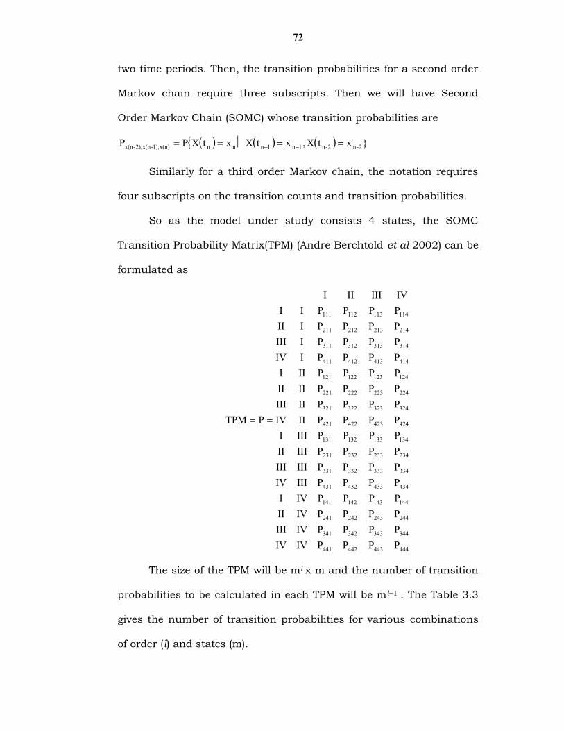
72

two time periods. Then, the transition probabilities for a second order

Markov chain require three subscripts. Then we will have Second

Order Markov Chain (SOMC) whose transition probabilities are

nnx(n)1),-x(n2),-x(n xtXPP }xtX,xtX 2-n2-n1n1n

Similarly for a third order Markov chain, the notation requires

four subscripts on the transition counts and transition probabilities.

So as the model under study consists 4 states, the SOMC

Transition Probability Matrix(TPM) (Andre Berchtold et al 2002) can be

formulated as

444443442441

344343342341

244243242241

144143142141

434433432431

334333332331

234233232231

134133132131

424423422421

324323322321

224223222221

124123122121

414413412411

314313312311

214213212211

114113112111

PPPPIVIVPPPPIVIIIPPPPIVIIPPPPIVIPPPPIIIIVPPPPIIIIIIPPPPIIIIIPPPPIIIIPPPPIIIVPPPPIIIIIPPPPIIIIPPPPIIIPPPPIIVPPPPIIIIPPPPIIIPPPPIIIVIIIIII

PTPM

The size of the TPM will be ml x m and the number of transition

probabilities to be calculated in each TPM will be ml+1 . The Table 3.3

gives the number of transition probabilities for various combinations

of order (l) and states (m).

73

Numberof

states(m)

Order (l) ofMarkovChain

Size oftheTPM

No. ofTransition

probabilities

2 1 2x2 42 4x2 83 8x2 164 16x2 32

3 1 3x3 92 9x3 273 27x3 814 81x3 243

4 1 4x4 162 16x4 643 64x4 2564 256x4 1024

Table 3.3: Number of transition probabilities for various combinationsof order (l) and states (m)

3.11 Parsimonious modeling of Higher order Markov Chain using

Weighted Moving Transition Probabilities

From the Table 3.3 it is evident that for higher order Markov

chain with more state space, the size of the TPM will be too large.

Estimation of several hundreds of parameters is a very time

consuming one. And also it will be difficult to analyse and make

conclusions or decisions.

Moreover as maintenance cost is in proportion of the items

falling in each state at certain time, the state probabilities are fairly

important rather through which intermediate states the current state

has been attained. Therefore focus on developing a model that yields

better forecast of the proportion of items in each state at a certain

time period is justifiable.

To address this, a parsimonious model, the Weighted Moving

Transition Probabilities (WMTP) method is introduced that

74

approximates higher order Markov chains. This makes the number of

parameters in each TPM to be computed far less. The size of the TPM

is m x m only. Each element of the TPM is the probability for the

occurrence of a particular event at time t given the probabilities of

immediate previous l (= order of the Markov Chain) time periods i.e.

at times from (t-l) to (t-1). The effect of each lag is considered by

assigning the weights.

For an l- order Markov Chain, in general, the probabilities can

be estimated as

nn xtXP }xtX,,xtX -n-n1n1n ll = g1g

ijg )(Pδ

l

subject to 11

l

gg and 0g .

is the weight parameter corresponding with the lag g. Pij are the

transition probabilities of the corresponding m x m TPM. It is based on

the premise that the most recent value is the most relevant to

estimate the future value; consequently the weights decrease as we

consider the older lags.

The weighted Moving Transition Probabilities-WMTP (for l = 2, Second

Order Markov process) can be written as:

nijP nn xtXP }xtX,xtX 2-n2-n1n1n

= g

2

1gijg )(Pδ

= 2nij2n1nij1n )(Pδ)(Pδ

where 1δδ 2n1n and ≥ 0.

75

As shown in the following Fig. 3.2 real Second Order Markov

Chain (SOMC) carries the combined influence of lags where as WMTP

model analogue carries the independent influences of each lag on the

present.

Fig. 3.2: Pictorial representation of Real SOMC and WMTP modeling of SOMC

Summary: Markov Process, a stochastic mathematical model, is used

in decision-making in the face of great amount of uncertainty. Markov

process is based on the premise that the future state of the system

depends on the current state but not on how it reaches the present

state. The general characteristics of the Markov Process, different

states of Markov process, order of Markov process, transition

probability etc. are discussed in detail. Stochastic matrix, eigen values

and eigen vectors of matrix, and spectral decomposition of a matrix

are also discussed.

By defining the higher order Multi state Markov processes and

the difficulties in estimating the corresponding transition

probabilities, reasons for introducing the Weighted Moving Transition

Probabilities (WMTP) technique are discussed in detail. Weighted

Moving Transition Probabilities (WMTP) technique is a parsimonious

model that approximates higher order Markov chains.

Xt-2 Xt-1 Xt

Xt-2 Xt-1 XtReal SOMC

WMTP modeling