markov decision processes: lecture notes for stp...
TRANSCRIPT

Markov Decision Processes: Lecture Notes for STP 425
Jay Taylor
November 26, 2012

Contents
1 Overview 4
1.1 Sequential Decision Models . . . . . . . . . . . . . . . . . . . . . . . . . . . . . . 4
1.2 Examples . . . . . . . . . . . . . . . . . . . . . . . . . . . . . . . . . . . . . . . . 5
2 Discrete-time Markov Chains 6
2.1 Formulation . . . . . . . . . . . . . . . . . . . . . . . . . . . . . . . . . . . . . . . 6
2.2 Asymptotic Behavior of Markov Chains . . . . . . . . . . . . . . . . . . . . . . . 11
2.2.1 Class Structure . . . . . . . . . . . . . . . . . . . . . . . . . . . . . . . . . 12
2.2.2 Hitting Times and Absorption Probabilities . . . . . . . . . . . . . . . . . 13
2.2.3 Stationary Distributions . . . . . . . . . . . . . . . . . . . . . . . . . . . . 15
3 Model Formulation 19
3.1 Definitions and Notation . . . . . . . . . . . . . . . . . . . . . . . . . . . . . . . . 19
3.2 Example: A One-Period Markov Decision Problem . . . . . . . . . . . . . . . . . 21
4 Examples of Markov Decision Processes 23
4.1 A Two-State MDP . . . . . . . . . . . . . . . . . . . . . . . . . . . . . . . . . . . 23
4.2 Single-Product Stochastic Inventory Control . . . . . . . . . . . . . . . . . . . . . 24
4.3 Deterministic Dynamic Programs . . . . . . . . . . . . . . . . . . . . . . . . . . . 26
4.4 Optimal Stopping Problems . . . . . . . . . . . . . . . . . . . . . . . . . . . . . . 27
4.5 Controlled Discrete-Time Dynamical Systems . . . . . . . . . . . . . . . . . . . . 30
4.6 Bandit Models . . . . . . . . . . . . . . . . . . . . . . . . . . . . . . . . . . . . . 31
4.7 Discrete-Time Queuing Systems . . . . . . . . . . . . . . . . . . . . . . . . . . . . 32
5 Finite-Horizon Markov Decision Processes 34
5.1 Optimality Criteria . . . . . . . . . . . . . . . . . . . . . . . . . . . . . . . . . . . 34
5.2 Policy Evaluation . . . . . . . . . . . . . . . . . . . . . . . . . . . . . . . . . . . . 36
5.3 Optimality Equations . . . . . . . . . . . . . . . . . . . . . . . . . . . . . . . . . 38
2

CONTENTS 3
5.4 Optimality of Deterministic Markov Policies . . . . . . . . . . . . . . . . . . . . . 42
5.5 The Backward Induction Algorithm . . . . . . . . . . . . . . . . . . . . . . . . . . 46
5.6 Examples . . . . . . . . . . . . . . . . . . . . . . . . . . . . . . . . . . . . . . . . 47
5.6.1 The Secretary Problem . . . . . . . . . . . . . . . . . . . . . . . . . . . . . 47
5.7 Monotone Policies . . . . . . . . . . . . . . . . . . . . . . . . . . . . . . . . . . . 49
6 Infinite-Horizon Models: Foundations 54
6.1 Assumptions and Definitions . . . . . . . . . . . . . . . . . . . . . . . . . . . . . . 54
6.2 The Expected Total Reward Criterion . . . . . . . . . . . . . . . . . . . . . . . . 56
6.3 The Expected Total Discounted Reward Criterion . . . . . . . . . . . . . . . . . . 57
6.4 Optimality Criteria . . . . . . . . . . . . . . . . . . . . . . . . . . . . . . . . . . . 59
6.5 Markov policies . . . . . . . . . . . . . . . . . . . . . . . . . . . . . . . . . . . . . 61
7 Discounted Markov Decision Processes 63
7.1 Notation and Conventions . . . . . . . . . . . . . . . . . . . . . . . . . . . . . . . 63
7.2 Policy Evaluation . . . . . . . . . . . . . . . . . . . . . . . . . . . . . . . . . . . . 65
7.3 Optimality Equations . . . . . . . . . . . . . . . . . . . . . . . . . . . . . . . . . 67
7.4 Value Iteration . . . . . . . . . . . . . . . . . . . . . . . . . . . . . . . . . . . . . 73
7.5 Policy Iteration . . . . . . . . . . . . . . . . . . . . . . . . . . . . . . . . . . . . . 77
7.6 Modified Policy Iteration . . . . . . . . . . . . . . . . . . . . . . . . . . . . . . . . 81

Chapter 1
Overview
1.1 Sequential Decision Models
This course will be concerned with sequential decision making under uncertainty, which we willrepresent as a discrete-time stochastic process that is under the partial control of an externalobserver. At each time, the state occupied by the process will be observed and, based on thisobservation, the controller will select an action that influences the state occupied by the systemat the next time point. Also, depending on the action chosen and the state of the system, theobserver will receive a reward at each time step. The key constituents of this model are thefollowing:
• a set of decision times (epochs);
• a set of system states (state space);
• a set of available actions;
• the state- and action-dependent rewards or costs;
• the state- and action-dependent transition probabilities on the state space.
Given such a model, we would like to know how the observer should act so as to maximize therewards, possibly subject to some constraints on the allowed states of the system. To this end,we will be interested in finding decision rules, which specify the action be chosen in a particularepoch, as well as policies, which are sequences of decision rules.
In general, a decision rule can depend not only on the current state of the system, but also onall previous states and actions. However, due to the difficulty of analyzing processes that allowarbitrarily complex dependencies between the past and the future, it is customary to focus onMarkov decision processes (MDPs), which have the property that the set of available actions,the rewards, and the transition probabilities in each epoch depend only on the current state ofthe system.
The principle questions that we will investigate are:
1. When does an optimal policy exist?
2. When does it have a particular form?
3. How can we efficiently find an optimal policy?
These notes are based primarily on the material presented in the book ‘Markov Decision Pro-cesses: Discrete Stochastic Dynamic Programming’ by Martin Puterman (Wiley, 2005).
4

1.2. EXAMPLES 5
1.2 Examples
Chapter 1 of Puterman (2005) describes several examples of how Markov decision processes canbe applied to real-world problems. I will describe just three of these in lecture, including:
1. Inventory management.
2. SIR models with vaccination (not in Puterman).
3. Evolutionary game theory: mate desertion by Cooper’s Hawks.

Chapter 2
Discrete-time Markov Chains
2.1 Formulation
A stochastic process is simply a collection of random variables {Xt : t ∈ T} where T is anindex set that we usually think of as representing time. We will say that the process is E-valuedif each of the variables Xt takes values in a set E. In this course we will mostly be concernedwith discrete-time stochastic processes and so we will usually consider sequences of variables ofthe form (Xn : n ≥ 0) or occasionally (Xn : n ∈ Z). Often we will interpret Xn to be thevalue of the process at time n, where time is measured in some specified units (e.g., days, years,generations, etc.), but in principle there is no need to assume that the times are evenly spacedor even that the index represents time.
When we model the time evolution of a physical system using a deterministic model, one desirableproperty is that the model should be dynamically sufficient. In other words, if we know that thesystem has state Xt = x at time t, then this should be sufficient to determine all future states ofthe system no matter how the system arrived at state x at time t. While dynamical sufficiency istoo much to ask for from a stochastic process, a reasonable counterpart would be to require thefuture states of the process to be conditionally independent of the past given the current stateXt = x. Stochastic processes that have this property are called Markov processes in generaland Markov chains in the special case that the state space E is either finite or countablyinfinite.
Definition 2.1. A stochastic process X = (Xn;n ≥ 0) with values in a set E is said to be adiscrete time Markov process if for every n ≥ 0 and every set of values x0, · · · , xn ∈ E, wehave
P (Xn+1 ∈ A|X0 = x0, X1 = x1, · · · , Xn = xn) = P (Xn+1 ∈ A|Xn = xn) , (2.1)
whenever A is a subset of E such that {Xn+1 ∈ A} is an event. In this case, the functions definedby
pn(x,A) = P(Xn+1 ∈ A|Xn = x)
are called the one-step transition probabilities of X. If the functions pn(x,A) do not dependon n, i.e., if there is a function p such that
p(x,A) = P(Xn+1 ∈ A|Xn = x)
for every n ≥ 0, then we say that X is a time-homogeneous Markov process with transitionfunction p. Otherwise, X is said to be time-inhomogeneous.
In light of condition (2.1), Markov processes are sometimes said to lack memory. More pre-cisely, it can be shown that this condition implies that conditional on the event {Xn = xn}, the
6

2.1. FORMULATION 7
variables (Xn+k; k ≥ 1) are independent of the variables (Xn−k; k ≥ 1), i.e., the future is condi-tionally independent of the past given the present. This is called the Markov property andwe will use it extensively in this course.
We can think about Markov processes in two ways. On the one hand, we can regard X =(Xn;n ≥ 0) as a collection of random variables that are all defined on the same probabilityspace. Alternatively, we can regard X itself as a random variable which takes values in the spaceof functions from N into E by defining
X(n) ≡ Xn.
In this case, X is said to be a function-valued or path-valued random variable and the particularsequence of values (xn;n ≥ 0) that the process assumes is said to be a sample path of X.
Example 2.1. Any i.i.d. sequence of random variables X1, X2, · · · is trivially a Markov process.Indeed, since all of the variables are independent, we have
P (Xn+1 ∈ A|X1 = x1, · · · , Xn = xn) = P (Xn+1 ∈ A) = p(xn, A),
and so the transition function p(x,A) does not depend on x.
Example 2.2. Discrete-time Random Walks
Let Z1, Z2, · · · be an i.i.d. sequence of real-valued random variables with probability density func-tion f(x) and define the process X = (Xn;n ≥ 0) by setting X0 = 0 and
Xn+1 = Xn + Zn+1.
X is said to be a discrete-time random walk and a simple calculation shows that X is a time-homogeneous Markov process on R with transition function
P (Xn+1 ∈ A|X0 = x0, · · · , Xn = x) = P (Xn+1 ∈ A|Xn = x)= P (Zn+1 − x ∈ A|Xn = x)= P (Zn+1 − x ∈ A)
=∫Af(z − x)dz.
One application of random walks is to the kinetics of particles moving in an ideal gas. Consider asingle particle and suppose that its motion is completely determined by a series of collisions withother particles present in the gas, each of which imparts a random quantity Z1, Z2, · · · to the ve-locity of the focal particle. Since particles move independently between collisions in ideal gases, thevelocity of the focal particle following the n’th collision will be given by the sum Xn = Z1+· · ·+Zn,implying that the velocity evolves as a random walk. Provided that the variables Zi have finitevariance, one prediction of this model (which follows from the Central Limit Theorem) is thatfor large n the velocity will be approximately normally distributed. Furthermore, if we extendthis model to motion in a three-dimensional vessel, then for large n the speed of the particle (theEuclidean norm of the velocity vector) will asymptotically have the Maxwell-Boltzmann distribu-tion. (Note: for a proper analysis of this model, we also need to consider the correlations betweenparticle velocities which arise when momentum is transferred from one particle to another.)
Random walks also provide a simple class of models for stock price fluctuations. For example, letYn be the price of a particular stock on day n and suppose that the price on day n+ 1 is given byYn+1 = Dn+1Yn, where D1, D2, · · · is a sequence of i.i.d. non-negative random variables. Thenthe variables Xn = log(Yn) will form a random walk with step sizes log(D1), log(D2), · · · . In thiscase, the CLT implies that for sufficiently large n, the price of the stock will be approximatelylog-normally distributed provided that the variables log(Di) have finite variance.

8 CHAPTER 2. DISCRETE-TIME MARKOV CHAINS
We can also construct a more general class of random walks by requiring the variables Z1, Z2, · · ·to be independent but not necessarily identically-distributed. For example, if each variable Znhas its own density fn, then the transition functions pn(x,A) will depend on n,
P (Xn+1 ∈ A|Xn = x) =∫Afn(y − x)dy,
and so the process X = (Xn;n ≥ 0) will be time-inhomogeneous. Time-inhomogeneous Markovprocesses are similar to ordinary differential equations with time-varying vector fields in thesense that the ‘rules’ governing the evolution of the system are themselves changing over time.If, for example, the variables Xn denote the position of an animal moving randomly in its hometerritory, then the distribution of increments could change as a function of the time of day orthe season of the year.
Definition 2.2. A stochastic process X = (Xn;n ≥ 0) with values in the countable set E ={1, 2, · · · } is said to be a time-homogeneous discrete-time Markov chain with initial dis-tribution ν and transition matrix P = (pij) if
1. for every i ∈ E, P (X0 = i) = νi;
2. for every n ≥ 0 and every set of values x0, · · · , xn+1 ∈ E, we have
P (Xn+1 = xn+1|X0 = x0, X1 = x1, · · · , Xn = xn) = P (Xn+1 = xn+1|Xn = xn)= pxnxn+1 .
In these notes, we will say that X is a DTMC for short.
Since pij is just the probability that the chain moves from i to j in one time step and sincethe variables Xn always take values in E, each vector pi = (pi1, pi2, · · · ) defines a probabilitydistribution on E and ∑
j∈Epij = P (X1 ∈ E|X0 = i) = 1
for every i ∈ E. In other words, all of the row sums of the transition matrix are equal to 1. Thismotivates our next definition.
Definition 2.3. Suppose that E is a countable (finite or infinite) index set. A matrix P = (pij)with indices ranging over E is said to be a stochastic matrix if all of the entries pij are non-negative and all of the row sums are equal to one:∑
j∈Epij = 1 for every i ∈ E.
Thus every transition matrix of a Markov chain is a stochastic matrix, and it can also be shownthat any stochastic matrix with indices ranging over a countable set E is the transition matrixfor a DTMC on E.
Remark 2.1. Some authors define the transition matrix to be the transpose of the matrix P thatwe have defined above. In this case, it is the column sums of P that are equal to one.

2.1. FORMULATION 9
Example 2.3. The transition matrix P of any Markov chain with values in a two state setE = {1, 2} can be written as
P =(
1− p pq 1− q
),
where p, q ∈ [0, 1]. Here p is the probability that the chain jumps to state 2 when it occupiesstate 1, while q is the probability that it jumps to state 1 when it occupies state 2. Notice that ifp = q = 1, then the chain cycles deterministically from state 1 to 2 and back to 1 indefinitely.
Theorem 2.1. Let X be a time-homogeneous DTMC with transition matrix P = (pij) and initialdistribution ν on E. Then
P (X0 = x0, X1 = x1, · · · , Xn = xn) = ν(x0)n−1∏i=0
pxi,xi+1 .
Proof. By repeated use of the Markov property, we have
P (X0 = x0, X1 = x1, · · · , Xn = xn) == P (X0 = x0, · · · , Xn−1 = xn−1) · P (Xn = xn|X0 = x0, · · · , Xn−1 = xn−1)= P (X0 = x0, · · · , Xn−1 = xn−1) · P (Xn = xn|Xn−1 = xn−1)= P (X0 = x0, · · · , Xn−1 = xn−1) · pxn−1,xn
= · · ·= P (X0 = x0, X1 = x1) · px1,x2 · · · pxn−1,xn
= P (X0 = x0) · P (X1 = x1|X0 = x0) · px1,x2 · · · pxn−1,xn
= ν(x0)n−1∏i=0
pxi,xi+1 ,
where ν(x0) is the probability of x0 under the initial distribution ν.
One application of Theorem (2.1) is to likelihood inference. For example, if the transition matrixof the Markov chain depends on a set of parameters, Θ, i.e., P = P (Θ), that we wish to estimateusing observations of a single chain, say x = (x0, · · · , xn), then the likelihood function will takethe form
L(Θ|x) = ν(x0)n−1∏i=0
p(Θ)xi,xi+1
,
and the maximum likelihood estimate of Θ will be the value of Θ that maximizes L(Θ|x).
The next theorem expresses an important relationship that holds between the n-step transitionprobabilities of a DTMC X and its r- and n − r-step transition probabilities. As the namesuggests, the n-step transition probabilities p(n)
ij of a DTMC X are defined for any n ≥ 1 by
p(n)ij = P (Xn = j|X0 = i) .
In fact, it will follow from this theorem that these too are independent of time whenever X istime-homogeneous, i.e., for every k ≥ 0,
p(n)ij = P (Xn+k = j|Xk = i) ,
which means that p(n)ij is just the probability that the chain moves from i to j in n time steps.

10 CHAPTER 2. DISCRETE-TIME MARKOV CHAINS
Theorem 2.2. (Chapman-Kolmogorov Equations) Assume that X is a time-homogeneousDTMC with n-step transition probabilities p(n)
ij . Then, for any non-negative integer r < n, theidentities
p(n)ij =
∑k∈E
p(r)ik p
(n−r)kj (2.2)
hold for all i, j ∈ E.
Proof. By using first the law of total probability and then the Markov property, we have
p(n)ij = P (Xn = j|X0 = i)
=∑k∈E
P (Xn = j,Xr = k|X0 = i)
=∑k∈E
P (Xn = j|Xr = k,X0 = i) · P (Xr = k|X0 = i)
=∑k∈E
P (Xn = j|Xr = k) · P (Xr = k|X0 = i)
=∑k∈E
p(r)ik p
(n−r)kj .
One of the most important features of the Chapman-Kolmogorov equations is that they can besuccinctly expressed in terms of matrix multiplication. If we write P (n) = (p(n)
ij ) for the matrixcontaining the n-step transition probabilities, then (2.2) is equivalent to
P (n) = P (r)P (n−r).
In particular, if we take n = 2 and r = 1, then since P (1) = P , we see that
P (2) = PP = P 2.
This, in turn, implies that P (3) = PP 2 = P 3, and continuing in this fashion shows that P (n) = Pn
for all n ≥ 1. Thus, the n-step transition probabilities of a DTMC can be calculated byraising the one-step transition matrix to the n’th power. This observation is importantfor several reasons, one being that if the state space is finite, then many of the properties of aMarkov chain can be deduced using methods from linear algebra.
Example 2.4. Suppose that X is the two-state Markov chain described in Example 2.3. Al-though the n-step transition probabilities can be calculated by hand in this example, we can moreefficiently calculate the powers of P by diagonalizing the transition matrix. In the following, wewill let d = p + q ∈ [0, 2]. We first solve for the eigenvalues of P , which are the roots of thecharacteristic equation:
λ2 − (2− d)λ+ (1− d) = 0
giving λ = 1 and λ = 1− d as the eigenvalues. As an aside, we note that any stochastic matrixP has λ = 1 as an eigenvalue and that v = (1, · · · , 1)T is a corresponding right eigenvector (hereT denotes the transpose). We also need to find a right eigenvector corresponding to λ = 1 − dand a direct calculation shows that v = (p,−q)T suffices. If we let Λ be the matrix formed fromthese two eigenvectors by setting
Λ =(
1 p1 −q
),
2.2. ASYMPTOTIC BEHAVIOR OF MARKOV CHAINS 11
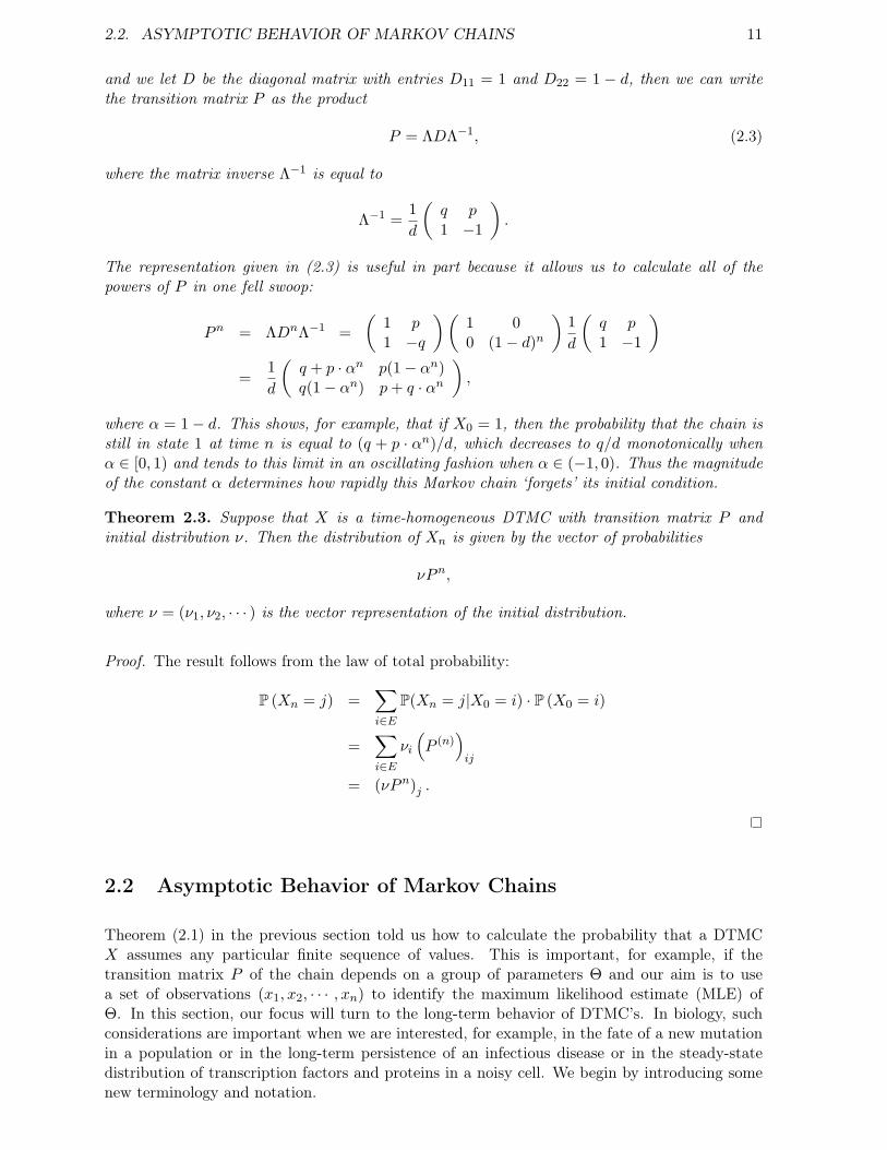
and we let D be the diagonal matrix with entries D11 = 1 and D22 = 1 − d, then we can writethe transition matrix P as the product
P = ΛDΛ−1, (2.3)
where the matrix inverse Λ−1 is equal to
Λ−1 =1d
(q p1 −1
).
The representation given in (2.3) is useful in part because it allows us to calculate all of thepowers of P in one fell swoop:
Pn = ΛDnΛ−1 =(
1 p1 −q
)(1 00 (1− d)n
)1d
(q p1 −1
)=
1d
(q + p · αn p(1− αn)q(1− αn) p+ q · αn
),
where α = 1− d. This shows, for example, that if X0 = 1, then the probability that the chain isstill in state 1 at time n is equal to (q + p · αn)/d, which decreases to q/d monotonically whenα ∈ [0, 1) and tends to this limit in an oscillating fashion when α ∈ (−1, 0). Thus the magnitudeof the constant α determines how rapidly this Markov chain ‘forgets’ its initial condition.
Theorem 2.3. Suppose that X is a time-homogeneous DTMC with transition matrix P andinitial distribution ν. Then the distribution of Xn is given by the vector of probabilities
νPn,
where ν = (ν1, ν2, · · · ) is the vector representation of the initial distribution.
Proof. The result follows from the law of total probability:
P (Xn = j) =∑i∈E
P(Xn = j|X0 = i) · P (X0 = i)
=∑i∈E
νi
(P (n)
)ij
= (νPn)j .
2.2 Asymptotic Behavior of Markov Chains
Theorem (2.1) in the previous section told us how to calculate the probability that a DTMCX assumes any particular finite sequence of values. This is important, for example, if thetransition matrix P of the chain depends on a group of parameters Θ and our aim is to usea set of observations (x1, x2, · · · , xn) to identify the maximum likelihood estimate (MLE) ofΘ. In this section, our focus will turn to the long-term behavior of DTMC’s. In biology, suchconsiderations are important when we are interested, for example, in the fate of a new mutationin a population or in the long-term persistence of an infectious disease or in the steady-statedistribution of transcription factors and proteins in a noisy cell. We begin by introducing somenew terminology and notation.

12 CHAPTER 2. DISCRETE-TIME MARKOV CHAINS
2.2.1 Class Structure
The terminology of this section is motivated by the observation that we can sometimes decom-pose the state space of a Markov chain into subsets called communicating classes on which thechain has relatively simple behavior.
Definition 2.4. Let X be a DTMC on E with transition matrix P .
1. We say that i leads to j, written i→ j, if for some integer n ≥ 0
p(n)ij = Pi (Xn = j) > 0.
In other words, i→ j if the process X beginning at X0 = i has some positive probability ofeventually arriving at j.
2. We say that i communicates with j, written i↔ j, if i leads to j and j leads to i.
It can be shown that the relation i↔ j is an equivalence relation on E:
1. Each element communicates with itself: i↔ j;
2. i communicates with j if and only if j communicates with i;
3. If i communicates with j and j communicates with k, then i communicates with k. Thisfollows from the Chapman-Kolmogorov equations by first choosing r and n so that p(r)
ij > 0
and p(n−r)jk > 0 (which we can do since i↔ j and j ↔ k), and then observing that
p(n)ik ≥ p
(r)ij p
(n−r)jk .
Our next definition is motivated by the fact that any equivalence relation on a set defines apartition of that set into equivalence classes: E = C1 ∪ C2 ∪ C3 ∪ · · · .
Definition 2.5. Let X be a DTMC on E with transition matrix P .
1. A nonempty subset C ⊂ E is said to be a communicating class if it is an equivalenceclass under the relation i↔ j. In other words, each pair of elements in C is communicating,and whenever i ∈ C and j ∈ E are communicating, j ∈ C.
2. A communicating class C is said to be closed if whenever i ∈ C and i → j, we also havej ∈ C. If C is a closed communicating class for a Markov chain X, then that means thatonce X enters C, it never leaves C.
3. A state i is said to be absorbing if {i} is a closed class, i.e., once the process enters statei, it is stuck there forever.
4. A Markov chain is said to be irreducible if the entire state space E is a communicatingclass.

2.2. ASYMPTOTIC BEHAVIOR OF MARKOV CHAINS 13
2.2.2 Hitting Times and Absorption Probabilities
In this section we will consider the following two problems. Suppose that X is a DTMC and thatC ⊂ E is an absorbing state or, more generally, any closed communicating class for X. Then twoimportant questions are: (i) what is the probability that X is eventually absorbed by A?; and(ii) assuming that this probability is 1, how long does it take on average for absorption to occur?For example, in the context of the Moran model without mutation, we might be interested inknowing the probability that A is eventually fixed in the population as well as the mean time forone or the other allele to be fixed. Clearly, the answers to these questions will typically dependon the initial distribution of the chain. Because the initial value X0 is often known, e.g., by directobservation or because we set it when running simulations, it will be convenient to introduce thefollowing notation. We will use Pi to denote the conditional distribution of the chain given thatX0 = i,
Pi (A) = P (A|X0 = i)
where A is any event involving the chain. Similarly, we will use Ei to denote conditional expec-tations given X0 = i,
Ei [Y ] = E [Y |X0 = i] ,
where Y is any random variable defined in terms of the chain.
Definition 2.6. Let X be a DTMC on E with transition matrix P and let C ⊂ E be a closedcommunicating class for X.
1. The absorption time of C is the random variable τC ∈ {0, 1, · · ·∞} defined by
τC =
min {n ≥ 0 : Xn ∈ C} if Xn ∈ C for some n ≥ 0
∞ if Xn /∈ C for all n.
2. The absorption probability of C starting from i is the probability
hCi = Pi(τC <∞
).
3. The mean absorption time by C starting from i is the expectation
kCi = Ei[τC].
The following theorem allows us, in principle, to calculate absorption probabilities by solving asystem of linear equations. When the state space is finite, this can often be done explicitly byhand or by numerically solving the equations. In either case, this approach is usually much fasterand more accurate than estimating the absorption probabilities by conducting Monte Carlo sim-ulations of the Markov chain.
Theorem 2.4. The vector of absorption probabilities hC = (hC1 , hC2 , · · · ) is the minimal non-
negative solution of the system of linear equations,{hCi = 1 if i ∈ ChCi =
∑j∈E pijh
Cj if i /∈ C
To say that hC is a minimal non-negative solution means that each value hCi ≥ 0 and that hCi ≤ xiif x = (x1, x2, · · · ) is another non-negative solution to this linear system.
14 CHAPTER 2. DISCRETE-TIME MARKOV CHAINS
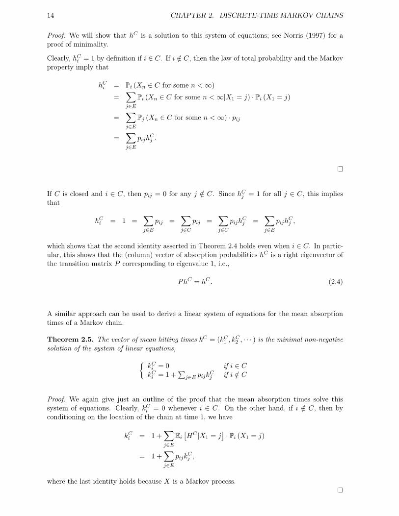
Proof. We will show that hC is a solution to this system of equations; see Norris (1997) for aproof of minimality.
Clearly, hCi = 1 by definition if i ∈ C. If i /∈ C, then the law of total probability and the Markovproperty imply that
hCi = Pi (Xn ∈ C for some n <∞)
=∑j∈E
Pi (Xn ∈ C for some n <∞|X1 = j) · Pi (X1 = j)
=∑j∈E
Pj (Xn ∈ C for some n <∞) · pij
=∑j∈E
pijhCj .
If C is closed and i ∈ C, then pij = 0 for any j /∈ C. Since hCj = 1 for all j ∈ C, this impliesthat
hCi = 1 =∑j∈E
pij =∑j∈C
pij =∑j∈C
pijhCj =
∑j∈E
pijhCj ,
which shows that the second identity asserted in Theorem 2.4 holds even when i ∈ C. In partic-ular, this shows that the (column) vector of absorption probabilities hC is a right eigenvector ofthe transition matrix P corresponding to eigenvalue 1, i.e.,
PhC = hC . (2.4)
A similar approach can be used to derive a linear system of equations for the mean absorptiontimes of a Markov chain.
Theorem 2.5. The vector of mean hitting times kC = (kC1 , kC2 , · · · ) is the minimal non-negative
solution of the system of linear equations,{kCi = 0 if i ∈ CkCi = 1 +
∑j∈E pijk
Cj if i /∈ C
Proof. We again give just an outline of the proof that the mean absorption times solve thissystem of equations. Clearly, kCi = 0 whenever i ∈ C. On the other hand, if i /∈ C, then byconditioning on the location of the chain at time 1, we have
kCi = 1 +∑j∈E
Ei[HC |X1 = j
]· Pi (X1 = j)
= 1 +∑j∈E
pijkCj ,
where the last identity holds because X is a Markov process.
2.2. ASYMPTOTIC BEHAVIOR OF MARKOV CHAINS 15
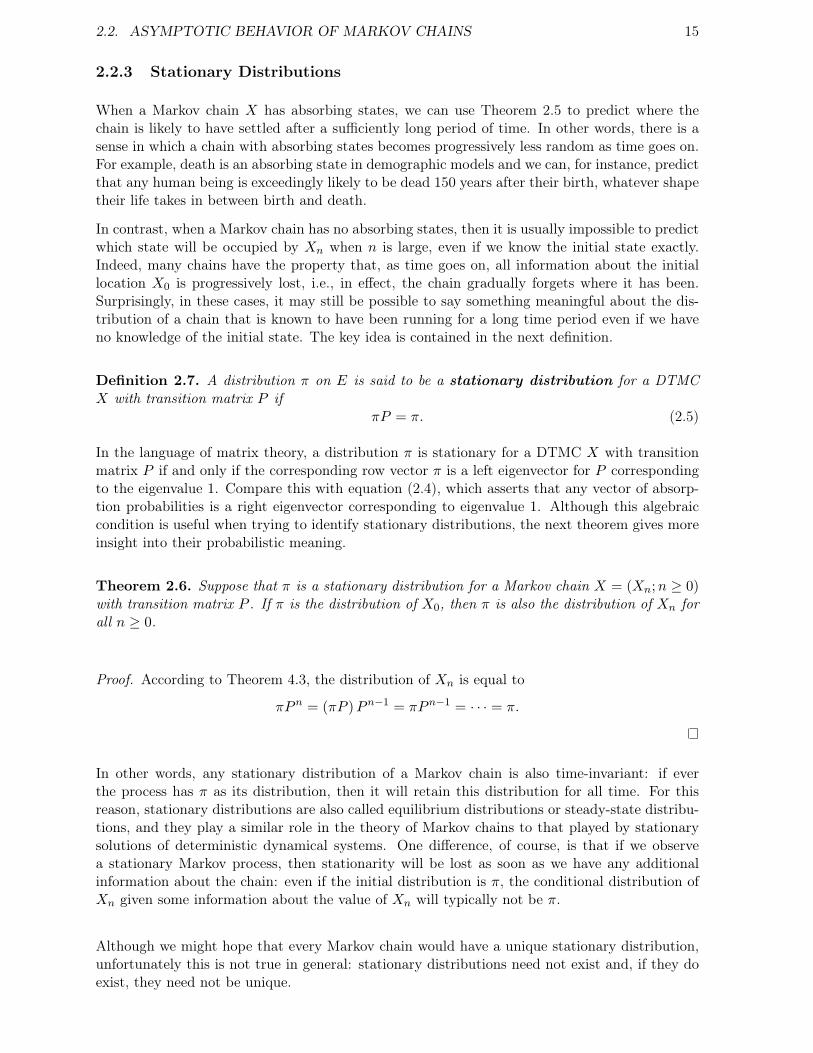
2.2.3 Stationary Distributions
When a Markov chain X has absorbing states, we can use Theorem 2.5 to predict where thechain is likely to have settled after a sufficiently long period of time. In other words, there is asense in which a chain with absorbing states becomes progressively less random as time goes on.For example, death is an absorbing state in demographic models and we can, for instance, predictthat any human being is exceedingly likely to be dead 150 years after their birth, whatever shapetheir life takes in between birth and death.
In contrast, when a Markov chain has no absorbing states, then it is usually impossible to predictwhich state will be occupied by Xn when n is large, even if we know the initial state exactly.Indeed, many chains have the property that, as time goes on, all information about the initiallocation X0 is progressively lost, i.e., in effect, the chain gradually forgets where it has been.Surprisingly, in these cases, it may still be possible to say something meaningful about the dis-tribution of a chain that is known to have been running for a long time period even if we haveno knowledge of the initial state. The key idea is contained in the next definition.
Definition 2.7. A distribution π on E is said to be a stationary distribution for a DTMCX with transition matrix P if
πP = π. (2.5)
In the language of matrix theory, a distribution π is stationary for a DTMC X with transitionmatrix P if and only if the corresponding row vector π is a left eigenvector for P correspondingto the eigenvalue 1. Compare this with equation (2.4), which asserts that any vector of absorp-tion probabilities is a right eigenvector corresponding to eigenvalue 1. Although this algebraiccondition is useful when trying to identify stationary distributions, the next theorem gives moreinsight into their probabilistic meaning.
Theorem 2.6. Suppose that π is a stationary distribution for a Markov chain X = (Xn;n ≥ 0)with transition matrix P . If π is the distribution of X0, then π is also the distribution of Xn forall n ≥ 0.
Proof. According to Theorem 4.3, the distribution of Xn is equal to
πPn = (πP )Pn−1 = πPn−1 = · · · = π.
In other words, any stationary distribution of a Markov chain is also time-invariant: if everthe process has π as its distribution, then it will retain this distribution for all time. For thisreason, stationary distributions are also called equilibrium distributions or steady-state distribu-tions, and they play a similar role in the theory of Markov chains to that played by stationarysolutions of deterministic dynamical systems. One difference, of course, is that if we observea stationary Markov process, then stationarity will be lost as soon as we have any additionalinformation about the chain: even if the initial distribution is π, the conditional distribution ofXn given some information about the value of Xn will typically not be π.
Although we might hope that every Markov chain would have a unique stationary distribution,unfortunately this is not true in general: stationary distributions need not exist and, if they doexist, they need not be unique.

16 CHAPTER 2. DISCRETE-TIME MARKOV CHAINS
Example 2.5. Let Z1, Z2, · · · be a sequence of i.i.d. Bernoulli random variables with successprobability p > 0 and let X = (Xn;n ≥ 0) be the random walk defined in Example 2.2: set X0 = 0and
Xn = Z1 + · · ·+ Zn.
Then Xn tends to infinity almost surely and X has no stationary distribution on the integers.
The problem that arises in this example is that as n increases, the probability mass ‘runs off toinfinity.’ This cannot happen when the state space is finite and, in fact, it can be shown that:
Theorem 2.7. Any DTMC X on a finite state space E has at least one stationary distribution.
Proof. Let P be the transition matrix of X. Since P is stochastic, 1 is the dominant eigenvalue ofP and then the Perron-Frobenius theorem tells us that there is a left eigenvector correspondingto 1 with non-negative entries. Normalizing this vector so that the entries sum to 1 supplies thestationary distribution π.
Recall from Definition 2.5 that a Markov chain is irreducible if all states in the state space arecommunicating, i.e., if the chain can move from any state i to any other state j in some finiteperiod of time. Under certain additional conditions, one can expect the distribution of an irre-ducible Markov chain starting from any initial distribution to tend to the same unique stationarydistribution as time passes. Sufficient conditions for this to be true are given in the next theorem,but we first need to introduce the following concept.
Definition 2.8. A DTMC X with values in E and transition matrix P is said to be aperiodicif for every state i ∈ E, p(n)
ii > 0 for all sufficiently large n.
Example 2.6. As the name suggests, an aperiodic chain is one in which there are no periodicorbits. For an example of a periodic Markov chain, take E = {1, 2} and let X be the chain withtransition matrix
P =(
0 11 0
).
If X0 = 1, then X2n = 1 and X2n+1 = 2 for all n ≥ 0, i.e., the chain simply oscillates betweenthe values 1 and 2 forever. Also, although π = (1/2, 1/2) is a stationary distribution for X, ifwe start the process with any distribution ν 6= π, then the distribution of Xn will never approachπ. Aperiodicity rules out the possibility of such behavior.
Theorem 2.8. Suppose that P is irreducible and aperiodic, and that π is a stationary distributionfor P . If µ is a distribution on E and X = (Xn;n ≥ 0) is a DTMC with transition matrix Pand initial distribution µ, then
limn→∞
P (Xn = j) = πj
for every j ∈ E. In particular,limn→∞
p(n)ij = πj
for all i, j ∈ E.

2.2. ASYMPTOTIC BEHAVIOR OF MARKOV CHAINS 17
In other words, any irreducible and aperiodic DTMC X has at most one stationary distributionand, if such a distribution π exists, then the distribution of the chain will tend to π no matterwhat the initial distribution was. Continuing the analogy with deterministic processes, such adistribution is analogous to a globally-attracting stationary solution of a dynamical system. Inpractice, the existence of such a stationary distribution means that if a system is modeled bysuch a Markov chain and if we have no prior knowledge of the state of the system, then it maybe reasonable to assume that the distribution of the state of the system is at equilibrium. Forexample, in population genetics, it has been common practice to assume that the distributionof allele frequencies is given by the stationary distribution of a Markov process when analyzingsequence data.
Example 2.7. Discrete-time birth and death processes
Let E = {0, · · · , N} for some N ≥ 1 and suppose that X = (Xn;n ≥ 0) is the DTMC withtransition matrix P = (pij) given by
P =
1− b0 b0 0 0 · · · 0 0 0d1 1− (b1 + d1) b1 0 · · · 0 0 00 d2 1− (b2 + d2) b2 · · · 0 0 0...
......
0 0 0 0 · · · dN−1 1− (bN−1 + dN−1) bN−1
0 0 0 0 · · · 0 dN 1− dN
.
X is said to be a (discrete-time) birth and death process and has the following interpretationif we think of Xn as the number of individuals present in the population at time n. If Xn =k ∈ {1, · · · , N − 1}, then there are three possibilities for Xn+1. First, with probability bk, oneof the individuals gives birth to a single offspring causing the population size to increase toXn+1 = k + 1. Secondly, with probability dk, one of the individuals dies and the population sizedecreases to Xn+1 = k − 1. Finally, with probability 1 − bk − dk, no individual reproduces ordies during that time step and so the population size remains at Xn+1 = k. The case Xn = 0needs a separate interpretation since clearly neither death nor birth can occur in the absence ofany individuals. One possibility is to let b0 be the probability that a new individual migrates intothe region when the population has gone extinct. Also, in this model we are assuming that whenXn = N , density dependence is so strong that no individual can reproduce. (It is also possible totake N =∞, in which case this is not an issue.)
If all of the birth and death probabilities bk, dk that appear in P are positive, then X is anirreducible, periodic DTMC defined on a finite state space and so it follows from Theorems 2.7and 2.8 that X has a unique stationary distribution π that satisfies the equation πP = π. Thisleads to the following system of equations,
(1− b0)π0 + d1π1 = π0
bk−1πk−1 + (1− bk − dk)πk + dk+1πk+1 = πk k = 1, · · · , N − 1bN−1πN−1 + (1− dN )πN = πN ,
which can be rewritten in the form
−b0π0 + d1π1 = 0bk−1πk−1 − (bk + dk)πk + dk+1πk+1 = 0 k = 1, · · · , N − 1
bN−1πN−1 − dNπN = 0.
The first equation can be rewritten as d1π1 = b0π0, which implies that
π1 =b0d1π0.

18 CHAPTER 2. DISCRETE-TIME MARKOV CHAINS
Taking k = 1, we haveb0π0 − d1π1 − b1π1 + d2π2 = 0.
However, since the first two terms cancel, this reduces to
−b1π1 + d2π2 = 0.
which shows thatπ2 =
b1d2π1 =
b1b0d2d1
π0.
Continuing in this way, we find that
πk =bk−1
dkπk−1 =
(bk−1 · · · b0dk · · · d1
)π0
for k = 1, · · · , N . All that remains to be determined is π0. However, since π is a probabilitydistribution on E, the probabilities must sum to one, which gives the condition
1 =N∑k=0
πk = π0
(1 +
N∑k=1
bk−1 · · · b0dk · · · d1
).
This forces
π0 =
(1 +
N∑k=1
bk−1 · · · b0dk · · · d1
)−1
(2.6)
and then
πk =(bk−1 · · · b0dk · · · d1
)1 +N∑j=1
bj−1 · · · b0dj · · · d1
−1
(2.7)
for k = 1, · · · , N .

Chapter 3
Model Formulation
3.1 Definitions and Notation
Recall that a Markov decision process (MDP) consists of a stochastic process along with adecision maker that observes the process and is able to select actions that influence its develop-ment over time. Along the way, the decision maker receives a series of rewards that depend onboth the actions chosen and the states occupied by the process. A MDP can be characterizedmathematically by a collection of five objects
{T, S,As, pt(·|s, a), rt(·|s, a) : t ∈ T, s ∈ S, a ∈ As}
which are described below.
(1) T ⊂ [0,∞) is the set of decision epochs, which are the points in time when the externalobserver decides on and then executes some action. We will mainly consider processes withcountably many decision epochs, in which case T is said to be discrete and we will usually takeT = {1, 2, · · · , N} or T = {1, 2, · · · } depending on whether T is finite or countably infinite. Timeis divided into time periods or stages in discrete problems and we assume that each decisionepoch occurs at the beginning of a time period. A MDP is said to have either a finite horizonor infinite horizon, respectively, depending on whether the least upper bound of T (i.e., thesupremum) is finite or infinite. If T = {1, · · · , N} is finite, we will stipulate that no decision istaken in the final decision epoch N .
(2) S is the set of states that can be assumed by the process and is called the state space. Scan be any measurable set, but we will mainly be concerned with processes that take values instate spaces that are either countable or which are compact subset of Rn.
(3) For each state s ∈ S, As is the set of actions that are possible when the state of the system iss. We will write A = ∪s∈SAs for the set of all possible actions and we will usually assume thateach As is either a countable set or a compact subset of Rn.
Actions can be chosen either deterministically or randomly. To describe the second possibility,we will write P(As) for the set of probability distributions on As, in which case a randomlychosen action can be specified by a probability distribution q(·) ∈ P(As), e.g., if As is discrete,then an action a ∈ As will be chosen with probability q(a).
(4) If T is discrete, then we must specify how the state of the system changes from one decisionepoch to the next. Since we are interested in Markov decision processes, these changes are chosenat random from a probability distribution pt(·|s, a) on S that may depend on the current timet, the current state of the system s, and the action a chosen by the observer.
(5) As a result of choosing action a when the system is in state s at time t, the observer receives
19
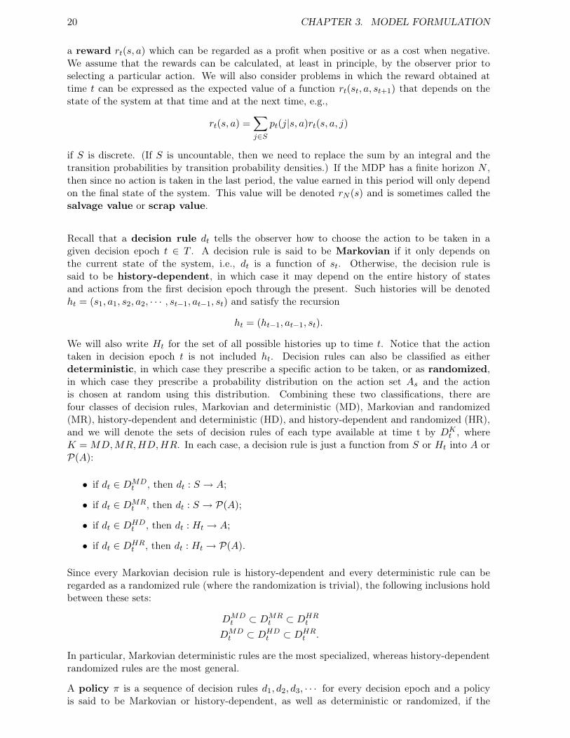
20 CHAPTER 3. MODEL FORMULATION
a reward rt(s, a) which can be regarded as a profit when positive or as a cost when negative.We assume that the rewards can be calculated, at least in principle, by the observer prior toselecting a particular action. We will also consider problems in which the reward obtained attime t can be expressed as the expected value of a function rt(st, a, st+1) that depends on thestate of the system at that time and at the next time, e.g.,
rt(s, a) =∑j∈S
pt(j|s, a)rt(s, a, j)
if S is discrete. (If S is uncountable, then we need to replace the sum by an integral and thetransition probabilities by transition probability densities.) If the MDP has a finite horizon N ,then since no action is taken in the last period, the value earned in this period will only dependon the final state of the system. This value will be denoted rN (s) and is sometimes called thesalvage value or scrap value.
Recall that a decision rule dt tells the observer how to choose the action to be taken in agiven decision epoch t ∈ T . A decision rule is said to be Markovian if it only depends onthe current state of the system, i.e., dt is a function of st. Otherwise, the decision rule issaid to be history-dependent, in which case it may depend on the entire history of statesand actions from the first decision epoch through the present. Such histories will be denotedht = (s1, a1, s2, a2, · · · , st−1, at−1, st) and satisfy the recursion
ht = (ht−1, at−1, st).
We will also write Ht for the set of all possible histories up to time t. Notice that the actiontaken in decision epoch t is not included ht. Decision rules can also be classified as eitherdeterministic, in which case they prescribe a specific action to be taken, or as randomized,in which case they prescribe a probability distribution on the action set As and the actionis chosen at random using this distribution. Combining these two classifications, there arefour classes of decision rules, Markovian and deterministic (MD), Markovian and randomized(MR), history-dependent and deterministic (HD), and history-dependent and randomized (HR),and we will denote the sets of decision rules of each type available at time t by DK
t , whereK = MD,MR,HD,HR. In each case, a decision rule is just a function from S or Ht into A orP(A):
• if dt ∈ DMDt , then dt : S → A;
• if dt ∈ DMRt , then dt : S → P(A);
• if dt ∈ DHDt , then dt : Ht → A;
• if dt ∈ DHRt , then dt : Ht → P(A).
Since every Markovian decision rule is history-dependent and every deterministic rule can beregarded as a randomized rule (where the randomization is trivial), the following inclusions holdbetween these sets:
DMDt ⊂ DMR
t ⊂ DHRt
DMDt ⊂ DHD
t ⊂ DHRt .
In particular, Markovian deterministic rules are the most specialized, whereas history-dependentrandomized rules are the most general.
A policy π is a sequence of decision rules d1, d2, d3, · · · for every decision epoch and a policyis said to be Markovian or history-dependent, as well as deterministic or randomized, if the

3.2. EXAMPLE: A ONE-PERIOD MARKOV DECISION PROBLEM 21
decision rules specified by the policy have the corresponding properties. We will write ΠK , withK = MD,MR,HD,HR, for the sets of policies of these types. A policy is said to be sta-tionary if the same decision rule is used in every epoch. In this case, π = (d, d, · · · ) for someMarkovian decision rule d and we denote this policy by d∞. Stationary policies can either bedeterministic or randomized and the sets of stationary policies of either type are denoted ΠSD
or ΠSR, respectively.
Because a Markov decision process is a stochastic process, the successive states and actionsrealized by that process form a sequence of random variables. We will introduce the followingnotation for these variables. For each t ∈ T , letXt ∈ S denote the state occupied by the system attime t and let Yt ∈ As denote the action taken at the start of that time period. It follows that anydiscrete-time process can be represented as a sequence of such variables X1, Y1, X2, Y2, X3, · · · .Likewise, we will define the history process Z = (Z1, Z2, · · · ) by setting Z1 = s1 and
Zt = (s1, a1, s2, a2, · · · , st).
The initial distribution of a MDP is a distribution on S and will be denoted P1(·). Furthermore,any randomized history-dependent policy π = (d1, d2, · · · , dN−1) induces a probability distribu-tion Pπ on the set of all possible histories (s1, a1, s2, a2, · · · , aN−1, sN ) according to the followingidentities:
Pπ{X1 = s1} = P1(s1),Pπ{Yt = a|Zt = ht} = qdt(ht)(a),
Pπ{Xt+1 = s|Zt = (ht−1, at−1, st), Yt = at} = pt(s|st, at).
Here qdt(ht) is the probability distribution on Ast which the decision rule dt uses to randomly selectthe next action at when the history of the system up to time t is given by ht = (ht−1, at−1, st). Theprobability of any particular sample path (s1, a1, · · · , aN−1, sN ) can be expressed as a productof such probabilities:
Pπ(s1, a1, · · · , aN−1, sN−1) = P1(s1)qd1(s1)(a1)p1(s2|s1, a1)qd2(h2)(a2)· · · qdN−1(hN−1)(aN−1)pN−1(sN |sN−1, aN−1).
If π is a Markovian policy, then the process X = (Xt : t ∈ T ) is a Markov process, as is theprocess (Xt, rt(Xt, Yt) : t ∈ T ), which we refer to as a Markov reward process. The Markovreward process tracks the states occupied the system as well as the sequence of rewards received.
3.2 Example: A One-Period Markov Decision Problem
By way of illustration, we describe a one-period MDP with T = {1, 2} and N = 2. We willassume that that the state space S is finite and also that the action sets As are finite for eachs ∈ S. Let r1(s, a) be the reward obtained when the system is in state s and action a is takenat the beginning of stage 1, and let v(s′) be the terminal reward obtained when the system isin state s′ at the end of this stage. Our objective is to identify policies that maximize the sumof r1(s, a) and the expected terminal reward. Since there is only one period, a policy consistsof a single decision rule and every history-dependent decision rule is also Markovian. (Here, asthroughout these lectures, we are assuming that the process begins at time t = 1, in which casethere is no prior history to be considered when deciding how to act during the first decisionepoch.)

22 CHAPTER 3. MODEL FORMULATION
If the observer chooses a deterministic policy π = (d1) and a′ = d1(s), then the total expectedreward when the initial system state is s is equal to
R(s, a′) ≡ r1(s, a′) + Eπs [v(X2)] = r1(s, a′) +∑j∈S
p1(j|s, a′)v(j),
where p1(j|s, a′) is the probability that the system occupies state j at time t = 2 given thatit was in state s at time t = 1 and action a′ was taken in this decision epoch. The observer’sproblem can be described as follows: for each state s ∈ S, find an action a∗ ∈ As that maximizesthe expected total reward, i.e., choose a∗s so that
R(s, a∗s) = maxa∈As
R(s, a).
Because the state space and action sets are finite, we know that there is at least one action a∗
that achieves this maximum, although it is possible that there may be more than one. It followsthat an optimal policy π = (d∗1) can be constructed by setting d∗1(s) = a∗s for each s ∈ S. Theoptimal policy will not be unique if there is a state s ∈ S for which there are multiple actionsthat maximize the expected total reward.
The following notation will sometimes be convenient. Suppose thatX is a set and that g : X → Ris a real-valued function defined on X. We will denote the set of points in X at which g ismaximized by
arg maxx∈X
g(x) ≡ {x′ ∈ X : g(x′) ≥ g(y) for all y ∈ X}.
If g fails to have a maximum on X, we will set arg maxx∈X g(x) = ∅. For example, if X = [−1, 1]and g(x) = x2, then
arg maxx∈[−1,1]
g(x) = {−1, 1}
since the maximum of g on this set is equal to 1 and −1 and 1 are the two points where g achievesthis maximum. In contrast, if X = (−1, 1) and g(x) = x2, then
arg maxx∈(−1,1)
g(x) = ∅
since g has no maximum on (−1, 1). With this notation, we can write
a∗s ∈ arg maxa′∈As
R(s, a′).
We next consider randomized decision rules. If the initial state of the system is s and the observerchooses action a ∈ As with probability q(a), then the expected total reward will be
Eq[R(s, ·)] =∑a∈As
q(a)R(s, a).
However, since
maxq∈P(As)
{∑a∈As
q(a)R(s, a)
}= max
a′∈AsR(s, a′),
it follows that a randomized rule can at best do as well as the best deterministic rule. In fact, arandomized rule with d(s) = qs(·) will do as well as the best deterministic rule if and only if foreach s ∈ S, ∑
a∗∈arg maxAs R(s,a∗)
qs(a∗) = 1.
In other words, the randomized rule should always select one of the actions that maximizes theexpected total reward.
Chapter 4
Examples of Markov Decision Processes
4.1 A Two-State MDP
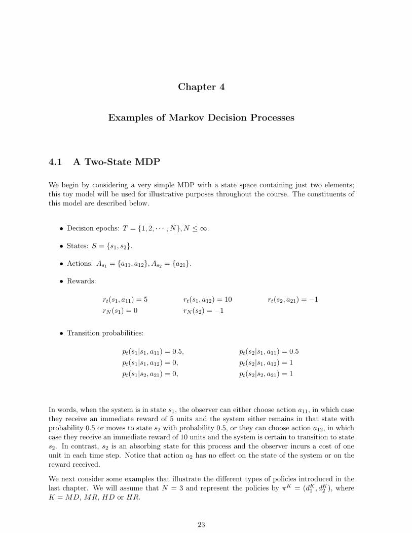
We begin by considering a very simple MDP with a state space containing just two elements;this toy model will be used for illustrative purposes throughout the course. The constituents ofthis model are described below.
• Decision epochs: T = {1, 2, · · · , N}, N ≤ ∞.
• States: S = {s1, s2}.
• Actions: As1 = {a11, a12}, As2 = {a21}.
• Rewards:
rt(s1, a11) = 5 rt(s1, a12) = 10 rt(s2, a21) = −1rN (s1) = 0 rN (s2) = −1
• Transition probabilities:
pt(s1|s1, a11) = 0.5, pt(s2|s1, a11) = 0.5pt(s1|s1, a12) = 0, pt(s2|s1, a12) = 1pt(s1|s2, a21) = 0, pt(s2|s2, a21) = 1
In words, when the system is in state s1, the observer can either choose action a11, in which casethey receive an immediate reward of 5 units and the system either remains in that state withprobability 0.5 or moves to state s2 with probability 0.5, or they can choose action a12, in whichcase they receive an immediate reward of 10 units and the system is certain to transition to states2. In contrast, s2 is an absorbing state for this process and the observer incurs a cost of oneunit in each time step. Notice that action a2 has no effect on the state of the system or on thereward received.
We next consider some examples that illustrate the different types of policies introduced in thelast chapter. We will assume that N = 3 and represent the policies by πK = (dK1 , d
K2 ), where
K = MD, MR, HD or HR.
23

24 CHAPTER 4. EXAMPLES OF MARKOV DECISION PROCESSES
A deterministic Markovian policy: πMD
Decision epoch 1: dMD1 (s1) = a11, dMD
1 (s2) = a21,
Decision epoch 2: dMD2 (s1) = a12, dMD
2 (s2) = a21.
A randomized Markovian policy: πMR
Decision epoch 1: qdMR1 (s1)(a11) = 0.7, qdMR
1 (s1)(a12) = 0.3
qdMR1 (s2)(a21) = 1.0;
Decision epoch 2: qdMR2 (s1)(a11) = 0.4, qdMR
2 (s1)(a12) = 0.6
qdMR2 (s2)(a21) = 1.0.
This model has the unusual property that the set of history-dependent policies is identical to theset of Markovian policies. This is true for two reasons. First, because the system can only remainin state s1 if the observer chooses action a11, there is effectively only one sample path ending ins1 in any particular decision epoch. Secondly, although there are multiple paths leading to states2, once the system enters this state, the observer is left with no choice regarding its actions.To illustrate history-dependent policies, we will modify the two-state model by adding a thirdaction a13 to A1,s1 which causes the system to remain in state s1 with probability 1 and providesa zero reward rt(s1, a13) = 0 for every t ∈ T . With this modification, there are now multiplehistories which can leave the system in state s1, e.g., (s1, a11, s1) and (s1, a13, s1).
A deterministic history-dependent policy: πHD
Decision epoch 1: dHD1 (s1) = a11, dMD1 (s2) = a21,
Decision epoch 2: dHD2 (s1, a11, s1) = a13, dHD2 (s1, a11, s2) = a21,
dHD2 (s1, a12, s1) = undefined, dHD2 (s1, a11, s2) = a21,
dHD2 (s1, a13, s1) = a11, dHD2 (s1, a13, s2) = undefined,
dHD2 (s2, a21, s1) = undefined, dHD2 (s2, a21, s2) = a21.
We leave the decision rules undefined when evaluated on histories that cannot occur, e.g., thehistory (s1, a12, s1) will never occur because the action a12 forces a transition from state s1 tostate s2. Randomized history-dependent policies can be defined in a similar manner.
4.2 Single-Product Stochastic Inventory Control
Suppose that a manager of a warehouse is responsible for maintaining the inventory of a singleproduct and that additional stock can be ordered from a supplier at the beginning of each month.The manager’s goal is to maintain sufficient stock to fill the random number of orders that willarrive each month, while limiting the costs of ordering and holding inventory. This problem canbe modeled by a MDP which we formulate using the following simplifying assumptions.
1. Stock is ordered and delivered at the beginning of each month.
2. Demand for the item arrives throughout the month, but orders are filled on the final dayof the month.
3. If demand exceeds inventory, the excess customers go to alternative source, i.e., unfilledorders are lost.

4.2. SINGLE-PRODUCT STOCHASTIC INVENTORY CONTROL 25
4. The revenues, costs and demand distribution are constant over time.
5. The product is sold only in whole units.
6. The warehouse has a maximum capacity of M units.
We will use the following notation. Let st denote the number of units in the warehouse at thebeginning of month t, let at be the number of units ordered from the supplier at the beginningof that month, and let Dt be the random demand during month t. We will assume that therandom variables D1, D2, · · · are independent and identically-distributed with distribution pj =P(Dt = j). Then the inventory at decision epoch t + 1 is related to the inventory at decisionepoch t through the following equation:
st+1 = max{st + at −Dt, 0} ≡ [st + at −Dt]+ .
The revenue and costs used to calculate the reward function are evaluated at the beginning ofeach month and are called present values. We will assume that the cost of ordering u units isequal to the sum of a fixed cost K > 0 for placing orders and a variable cost c(u) that increaseswith the number of units ordered, i.e.,
O(u) =
0 if u = 0
K + c(u) if u > 0.
Likewise, let h(u) be a non-decreasing function that specifies the cost of maintaining an inventoryof u units for a month and let g(u) be the value of any remaining inventory in the last decisionepoch of a finite horizon model. Finally, let f(j) be the revenue earned from selling j units ofinventory and assume that f(0) = 0. Assuming that the revenue is only gained at the end of themonth when the month’s orders are filled, the reward depends on the state of the system at thestart of the next decision epoch:
rt(st, at, st+1) = −O(at)− h(st + at) + f(st + at − st+1).
However, since st+1 is still unknown during decision epoch t, it will be more convenient to workwith the expected present value at the beginning of the month of the revenue earned throughoutthat month. This will be denoted F (u), where u is the number of units present at the beginningof month t, and is equal to
F (u) =u−1∑j=0
pjf(j) + quf(u),
where
qu =∞∑j=u
pj = P(Dt ≥ u)
is the probability that the demand equals or exceeds the available inventory.
The MDP can now be formulated as follows:
• Decision epochs: T = {1, 2, · · · , N}, N ≤ ∞;
• States: S = {0, 1, · · · ,M};
• Actions: As = {0, 1, · · · ,M − s};
26 CHAPTER 4. EXAMPLES OF MARKOV DECISION PROCESSES
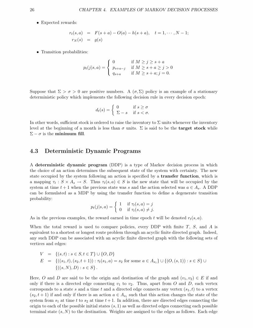
• Expected rewards:
rt(s, a) = F (s+ a)−O(a)− h(s+ a), t = 1, · · · , N − 1;rN (s) = g(s)
• Transition probabilities:
pt(j|s, a) =
0 if M ≥ j ≥ s+ aps+a−j if M ≥ s+ a ≥ j > 0qs+a if M ≥ s+ a; j = 0.
Suppose that Σ > σ > 0 are positive numbers. A (σ,Σ) policy is an example of a stationarydeterministic policy which implements the following decision rule in every decision epoch:
dt(s) ={
0 if s ≥ σΣ− s if s < σ.
In other words, sufficient stock is ordered to raise the inventory to Σ units whenever the inventorylevel at the beginning of a month is less than σ units. Σ is said to be the target stock whileΣ− σ is the minimum fill.
4.3 Deterministic Dynamic Programs
A deterministic dynamic program (DDP) is a type of Markov decision process in whichthe choice of an action determines the subsequent state of the system with certainty. The newstate occupied by the system following an action is specified by a transfer function, which isa mapping τt : S × As → S. Thus τt(s, a) ∈ S is the new state that will be occupied by thesystem at time t+ 1 when the previous state was s and the action selected was a ∈ As. A DDPcan be formulated as a MDP by using the transfer function to define a degenerate transitionprobability:
pt(j|s, a) ={
1 if τt(s, a) = j0 if τt(s, a) 6= j.
As in the previous examples, the reward earned in time epoch t will be denoted rt(s, a).
When the total reward is used to compare policies, every DDP with finite T , S, and A isequivalent to a shortest or longest route problem through an acyclic finite directed graph. Indeed,any such DDP can be associated with an acyclic finite directed graph with the following sets ofvertices and edges:
V = {(s, t) : s ∈ S, t ∈ T} ∪ {O,D}E = {((s1, t), (s2, t+ 1)) : τt(s1, a) = s2 for some a ∈ As1} ∪ {(O, (s, 1)) : s ∈ S} ∪
{((s,N), D) : s ∈ S} .
Here, O and D are said to be the origin and destination of the graph and (v1, v2) ∈ E if andonly if there is a directed edge connecting v1 to v2. Thus, apart from O and D, each vertexcorresponds to a state s and a time t and a directed edge connects any vertex (s1, t) to a vertex(s2, t+ 1) if and only if there is an action a ∈ As1 such that this action changes the state of thesystem from s1 at time t to s2 at time t+ 1. In addition, there are directed edges connecting theorigin to each of the possible initial states (s, 1) as well as directed edges connecting each possibleterminal state (s,N) to the destination. Weights are assigned to the edges as follows. Each edge

4.4. OPTIMAL STOPPING PROBLEMS 27
connecting a vertex (s1, t) to a vertex (s2, t + 1) and corresponding to an action a is assigneda weight equal to the reward rt(s, a). Likewise, each edge connecting a terminal state (s,N) toD is assigned a weight equal to the reward rN (s). Finally, each edge connecting the origin to apossible initial state (s, 1) is assigned a weight either equal to L� 1 if s is the actual initial stateand equal to 0 otherwise. Choosing a policy that maximizes the total reward is equivalent tofinding the longest route through this graph from the origin to the destination. As explained onp. 43 of Puterman (2005), the longest route problem is also central to critical path analysis.
Certain kinds of sequential allocation models can be interpreted as deterministic dynamicprograms. In the general formulation of a sequential allocation model, a decision maker has afixed quantity M of resources to be consumed or used in some manner over N periods. Let xtdenote the quantity of resources consumed in period t and suppose that f(x1, · · · , xN ) is theutility (or reward) for the decision maker of the allocation pattern (x1, · · · , xN ). The problemfaced by the decision maker is to choose an allocation of the resources that maximizes the utilityf(x1, · · · , xN ) subject to the constraints
x1 + · · ·+ xN = M
xt ≥ 0, t = 1, · · · , N.
Such problems are difficult to solve in general unless the utility function has special propertiesthat can be exploited, either analytically or numerically, in the search for the global maximum.For example, the utility function f(x1, · · · , xN ) is said to be separable if it can be written as asum of univariate functions of the form
f(x1, · · · , xN ) =N∑t=1
gt(xi),
where gt : [0,M ] → R is the utility gained from utilizing xt resources during the t’th periodand we assume that gt is a non-decreasing function of its argument. In this case, the sequentialallocation model can be formulated as a DDP/MDP as follows:
• Decision epochs: T = {1, · · · , N};
• States: S = [0,M ];
• Actions: As = [0, s];
• Rewards: rt(s, a) = gt(a);
• Transition probabilities:
pt(j|s, a) ={
1 if j = s− a0 otherwise .
There are also stochastic versions of this problem in which either the utility or the opportunityto allocate resources in each time period is random.
4.4 Optimal Stopping Problems
We first formulate a general class of optimal stopping problems and then consider specific ap-plications. In the general problem, a system evolves according to an uncontrolled Markov chainwith values in a state space S′ and the only actions available to the decision maker are to eitherdo nothing, in which case a cost ft(s) is incurred if the system is in state s at time t, or to stopthe chain, in which case a reward gt(s) is received. If the process has a finite horizon, then the

28 CHAPTER 4. EXAMPLES OF MARKOV DECISION PROCESSES
decision maker received a reward h(s) if the unstopped process is in state s at time N . Oncethe chain is stopped, there are no more actions or rewards. We can formulate this problem as aMDP as follows:
• Decision epochs: T = {1, · · · , N}, N ≤ ∞.
• States: S = S′ ∪ {∆}.
• Actions:
As ={{C,Q} if s ∈ S′{C} if s = ∆.
• Rewards:
rt(s, a) =
−ft(s) if s ∈ S′, a = Cgt(s) if s ∈ S′, a = Q, (t < N)0 if s = ∆
rN (s) = h(s).
• Transition probabilities:
pt(j|s, a) =
pt(j|s) if s, j ∈ S′, a = C1 if s ∈ S′, j = ∆, a = Q1 if s = j = ∆, a = C0 otherwise.
Here ∆ is an absorbing state (sometimes called a cemetery state) that is reached only if thedecision maker decides to stop the chain. This is added to the state space S′ of the originalchain to give the extended state space S. While the chain is in S′, two actions are available tothe decision maker: either to continue the process (C) or to quit it (Q). Continuation allowsthe process to continue to evolve in S′ according to the transition matrix of the Markov chain,while quitting causes the process to move to the cemetery state where it remains forever. Theproblem facing the decision maker is to find a policy that will specify when to quit the processin such a way that maximizes the difference between the gain at the stopping time and the costsaccrued up to that time.
Example 4.1. Selling an asset. Suppose that an investor owns an asset (such as a property)the value of which fluctuates over time and which must be sold by some final time N . Let Xt
denote the price at time t, where time could be measured in days, weeks, months or any otherdiscrete time unit, and assume that X = (X1, X2, · · · : t ≥ 0) is a Markov process with valuesin the set S′ = [0,∞). If the investor retains the asset in the t’th period, then she will incur acost ft(s) that includes property taxes, advertising costs, etc. If the investor chooses to sell theproperty in the t’th decision epoch, then she will earn a profit s−K(s) where s = Xt is the valueof the asset at that time and K(s) is the cost of selling the asset at that price. If the property isstill held at time N , then it must be sold at a profit (or loss) of s−K(s), where s = XN is thefinal value.
Optimal policies for this problem often take the form of control limit policies which havedecision rules of the following form:
dt(s) ={Q if s ≥ BtC if s < Bt.
Here Bt is the control limit at time t and its value will usually change over time.

4.4. OPTIMAL STOPPING PROBLEMS 29
Example 4.2. The Secretary Problem. Suppose that an employer seeks to fill a vacancyfor which there are N candidates. Candidates are interviewed sequentially and following eachinterview, the employer must decide whether or not to offer the position to the current candidate.If the employer does not offer them the position, then that individual is removed from the poolof potential candidates and the next candidate is interviewed. There are many variations on thisproblem, but here we will assume that the candidates can be unambiguously ranked from best toworst and that the employer’s objective is to maximize the probability of offering the job to themost-preferred candidate.
We can reformulate the problem as follows. Suppose that a collection of N objects is ranked from1 to N and that the lower the ranking the more preferred the object is. An observer encountersthese objects sequentially, one at a time, in a random order, where each of the N ! possible ordersis equally likely to occur. Although the absolute rank of each object is unknown to the observer,the relative ranks are known without error, e.g., the observer can tell whether the second objectencountered is more or less preferred than the first object, but the observer cannot determine atthat stage whether the first or second object is the best in the entire group of N if N > 2.
To cast this problem as a MDP, we will let T = {1, · · · , N} and S′ = {0, 1}, where st = 1indicates that the t’th object observed is the best one encountered so far and st = 0 indicatesthat a better object was encountered at an earlier time. If t < N , then the observer can eitherselect the current object and quit (Q) or they can reject the current object and proceed to thenext one in the queue (C). If t = N , then the observer is required to select the last object in thequeue. We will assume that there are no continuation costs, i.e., ft(0) = ft(1) = 0, and we willtake the reward at stopping gt(s) to be equal to be equal to the probability of choosing the bestobject in the group. Notice that the terminal reward h(s) = gN (s) is equal to 1 if s = 1 and 0otherwise. Indeed, the N ’th object will be the best one in the group if and only if it is the best oneencountered. Furthermore, gt(0) = 0 for all t = 1, · · · , N , since if we select an object for whichst = 0, then that means that we know that there is another object in the group that is better thanthe one that we are selecting. To calculate gt(1), we first observe that because we are equallylikely to observe the objects in any order, the conditional probability that the t’th object is the bestin the group given that it is the best in the first t objects observed is equal to the probability thatthe best object in the group is one of the first t objects encountered. Accordingly,
gt(1) = P(the best object in the first t objects is the best overall
)=
number of subsets of {1, · · · , N} of size t containing 1number of subsets of {1, · · · , N} of size t
=
(N−1t−1
)(Nt
) =t
N.
Again because of permutation invariance, the transition probabilities pt(j|s) do not depend on thecurrent state. Instead, the probability that the t+ 1’st object encountered is the best amongst firstt+ 1 objects is equal to 1/(t+ 1) and so
pt(j|s) ={ 1
t+1 if j = 1tt+1 if j = 0,
for both s = 0 and s = 1.
Similar problems arise in behavioral ecology, where an individual of the ‘choosy sex’ sequentiallyencounters individuals of the opposite sex and must choose whether to mate with the t’th individualor defer mating until a subsequent encounter with a different individual.

30 CHAPTER 4. EXAMPLES OF MARKOV DECISION PROCESSES
4.5 Controlled Discrete-Time Dynamical Systems
We consider a class of stochastic dynamical systems that are governed by a recursive equationof the following form:
st+1 = ft(st, ut, wt), (4.1)
where st ∈ S is the state of the system at time t, ut ∈ U is the control used at time t, and wt ∈Wis the disturbance of the system at time t. As above, S is called the state space of the system,but now we also have a control set U as well as a disturbance set W . Informally, we canthink of the sequence s0, s1, · · · as a deterministic dynamical system that is perturbed both by asequence of control actions u0, u1, · · · chosen by an external observer (the ‘controller’) as well asby a sequence of random disturbances w0, w1, · · · that are not under the control of that observer.To be concrete, we will assume that S ⊂ Rk, U ⊂ Rm, andW ⊂ Rn, and that f : S×U×W → Smaps triples (s, u, w) into S. We will also assume that the random disturbances are governedby a sequence of independent random variables W0,W1, · · · with values in the set W and wewill let qt(·) be the probability mass function or the probability density function of Wt. Whenthe system is in state st and a control ut is chosen from a set Us ⊂ U of admissible control instate s, then the controller will receive a reward gt(s, u). In addition, if the horizon is finite andthe system terminates in state sN at time N , then the controller will receive a terminal rewardgN (sN ) that depends only on the final state of the system. We can formulate this problem as aMDP as follows:
• Decision epochs: T = {1, · · · , N}, N ≤ ∞.
• States: S ⊂ Rk.
• Actions: As = Us ⊂ U ⊂ Rm.
• Rewards:
rt(s, a) = gt(s, a), t < N
rN (s) = gN (s).
• Transition probabilities (discrete noise):
pt(j|s, a) = P(j = ft(s, a,Wt)
)=
∑{w∈W :j=ft(s,a,w)}
qt(w).
(If the disturbances are continuously-distributed, then the sum appearing in the transition prob-ability must be replaced by an integral.)
The only substantial difference between a controlled discrete-time dynamical system and aMarkov decision process is in the manner in which randomness is incorporated. Whereas MDPsare defined using transition probabilities that depend on the current state and action, the tran-sition probabilities governing the behavior of the dynamical system corresponding to equation(4.1) must be derived from the distributions of the disturbance variables Wt. In the languageof control theory, a decision rule is called a feedback control and open loop control is adecision rule which does not depend on the state of the system, i.e., dt(s) = a for all s ∈ S.
Example 4.3. Economic growth models. We formulate a simple stochastic dynamical modelfor a planned economy in which capital can either be invested or consumed. Let T = {1, 2, · · · }be time measured in years and let st ∈ S = [0,∞) denote the capital available for investment inyear t. (By requiring st ≥ 0, we stipulate that the economy is debt-free.) After observing the level

4.6. BANDIT MODELS 31
of capital available at time t, the planner chooses a level of consumption ut ∈ Ust = [0, st] andinvests the remaining capital st−ut. Consumption generates an immediate utility Ψt(st) and theinvestment produces capital for the next year according to the dynamical equation
st+1 = wtFt(st − ut)
where Ft determines the expected return on the investment and wt is a non-negative randomvariable with mean 1 that accounts for disturbances caused by random shocks to the system, e.g.,due to climate, political instability, etc.
4.6 Bandit Models
In a bandit model the decision maker observesK independent Markov processesX(1), · · · , X(K)
and at each decision epoch selects one of these processes to use. If the process i is chosen at timet when it is in state si ∈ Si, then
1. the process i moves from state si to state ji according to the transition probability pit(ji|si);
2. the decision maker receives a reward rit(si);
3. all other processes remain in their current states.
Usually, the decision maker wishes to choose a sequence of processes in such a way that maximizesthe total expected reward or some similar objective function. We can formulate this as a Markovdecision process as follows:
• Decision epochs: T = {1, 2, · · · , N}, N ≤ ∞.
• States: S = S1 × S2 × · · · × SK .
• Actions: As = {1, · · · ,K}.
• Rewards: rt((s1, · · · , SK), i) = rit(si).
• Transition probabilities:
pt((u1, · · · , uK)|(s1, · · · , sK), i) ={p(ji|si) if ui = ji and um = sm for all m 6= i0 if um 6= sm.
There are numerous variations on the basic bandit model, including restless bandits which al-low the states of the unselected processes to change between decision epochs and arm-acquiringbandits which allow the number of processes to increase or decrease at each decision epoch.
Example 4.4. Gambling. Suppose that a gambler in a casino can pay c units to pull the leveron one of K slot machines and that the i’th machine pays 1 unit with probability qi and 0 unitswith probability 1 − qi. The values of the probabilities qi are unknown, but the gambler gainsinformation concerning the distribution of qi each time that she chooses to play the game usingthe i’th machine. The gambler seeks to maximize her expected winnings, but to do so, she faces atradeoff between exploiting the machine that appears to be best based on the information collectedthus far and exploring other machines that might have higher probabilities of winning.
This problem can be formulated as a multi-armed bandit problem as follows. For each i =1, · · · ,K, let Si be the space of probability density functions defined on [0, 1] and let sit = f ∈ Si

32 CHAPTER 4. EXAMPLES OF MARKOV DECISION PROCESSES
if the density of the posterior distribution of the value of qi given the data available up to time tis equal to f(q). At time t = 1, the gambler begins by choosing a set of prior distributions for thevalues of the qi’s; these can be based on previous experience with these or similar slot machines,or they can be chosen to be ‘uninformative’. At each decision epoch t, the gambler can choose toplay the game using one of the K machines. If the i’th machine is chosen and if the posteriordensity for the value of qi at that time is sit = f , then the expected reward earned in that periodis equal to
rt((s1, · · · , sK), i) = E[Q]− c =∫ 1
0qf(q)− c,
where Q is a [0, 1]-valued random variable with density f(q).
Let W be an indicator variable for the event that the gambler wins when betting with slot machinei at time t, i.e., W = 1 if the gambler wins and W = 0 otherwise. Then the distribution of qi atdecision epoch t+ 1 depends on the value of W , and Bayes’ formula can be used to calculate theposterior density f ′ of qi given W :
f ′(qi|W ) =qWi (1− qi)1−W f(qi)∫ 10 q
W (1− q)W f(q)dq.
In other words, if the gambler wins when using the i’th machine, then she updates the density of qifrom f to qif(qi)/Ef [Q] and this occurs with probability Ef [Q]. On the other hand, if the gamblerloses when using this machine, then she updates the distribution to (1− qi)f(qi)/Ef [1−Q] andthis occurs with probability 1−Ef [Q]. In the meantime, the distributions of the other probabilitiesqj , j 6= i, do not change when i is played.
Due to the sequential nature of the updating, the state spaces used to represent the gambler’sbeliefs concerning the values of the qi can be simplified to Si = N × N. For each i = 1, · · · ,K,let fi,0(qi) be the density of the gambler’s prior distribution for qi and let Wi,t and Li,t be thenumber of times that the gambler has either won or lost, respectively, using the i’th slot machineup to time t. Then the density of the posterior distribution for qi given the sequence of wins andlosses depends only on the numbers Wi,t and Li,t and is equal to
fi,t(qi|Wi,t, Li,t) =qWi,t
i (1− qi)Li,tfi,0(qi)∫ 10 q
Wi,t(1− q)Li,tfi,0(q)dq.
Variations of the multi-armed bandit model described in the previous example have been usedto design sequential clinical trials. Patients sequentially enter a clinical trial and are assigned toone of K groups receiving different treatments. The aim is to find the most effective treatmentwhile causing the least harm (or giving the greatest benefit) to the individuals enrolled in thetrial.
4.7 Discrete-Time Queuing Systems
Controlled queuing systems can be studied using the machinery of MDPs. In an uncontrolledsingle-server queue, jobs arrive, enter the queue, wait for service, receive service, and then aredischarged from the system. Controls can be added which either regulate the number of jobsthat are admitted to the queue (admission control) or which adjust the service rate (service ratecontrol).
Here we will consider admission control. In these models, jobs arrive for service and are placedinto a ‘potential job queue.’ At each decision epoch, the controller observes the number of jobsin the system and then decides how many jobs to admit from the potential queue to the eligible

4.7. DISCRETE-TIME QUEUING SYSTEMS 33
queue. Jobs not admitted to the eligible queue never receive service. To model this as a MDP,let Xt denote the number of jobs in the system just before decision epoch t and let Zt−1 be thenumber of jobs arriving in period t− 1 and entering the potential job queue. At decision epocht, the controller admits ut jobs from the potential job queue into the eligible job queue. Let Ytbe the number of possible service completions and notice that the actual number of completionsis equal to the minimum of Yt and Xt + ut, the latter quantity being the number of jobs in thesystem at time t that can be serviced during this period.
The state of the system at decision epoch t can be represented by a pair (Xt, Vt), where Vt isthe number of jobs in the potential queue at that time. These variables satisfy the followingdynamical equation:
Xt+1 = [Xt + ut − Yt]+
Vt+1 = Zt,
where 0 ≤ ut ≤ Vt, since only jobs in the potential queue can be admitted to the system.Here we will assume that the integer-valued variables Y1, Y2, · · · are i.i.d. with probability massfunction f(n) = P(Yt = n) and likewise that Z1, Z2, · · · are i.i.d. with probability mass functiong(n) = P(Z1 = n). We will also assume that there is both a constant reward of R units for everycompleted job and a holding cost of h(x) per period when there are x jobs in the system.
To formulate this as a MDP, let
• Decision epochs: T = {0, 1, · · · , N}, N ≤ ∞.
• States: S = S1 × S2 = N× N, where s1 is the number in the system and s2 is the numberin the potential job queue.
• Actions: As1,s2 = {0, 1, · · · , s2}.
• Rewards:rt(s1, s2, a) = R · E[min(Yt, s1 + a)]− h(s1 + a)
• Transition probabilities:
pt(s′1, s′2|s1, s2, a) =
f(s1 + a− s′1)g(s′2) if a+ s1 > s′1 > 0[∑∞
i=s1+a f(i)]g(s′2) if s′1 = 0, a+ s1 > 0
g(s′2) if s′1 = a+ s1 = 00 if s′1 > a+ s1 ≥ 0.

Chapter 5
Finite-Horizon Markov Decision Processes
5.1 Optimality Criteria
Recall that a discrete-time Markov decision process is said to be a finite-horizon process if theset of decision epochs is finite. Without loss of generality, we will take this set to be T ={1, 2, · · · , N}, where N <∞. We also recall the following notation from Chapter 2:
• S is the state space.
• As is the set of possible actions when the system is in state s; A = ∪s∈SAs is the set of allpossible actions.
• rt(s, a) is the reward earned when the system is in state s and action a is selected in decisionepoch t ∈ {1, · · · , N −1}. rN (s) is the reward earned if the system is in state s at the finaltime t = N .
• pt(j|s, a) is the transition probability from state s at time t to state j at time t+ 1 whenaction a is selected in decision epoch t.
Further, we will write ht = (s1, a1, s2, a2, · · · , st) for the history of the process up to time t andwe will let Ht be the set of all possible histories up to time t. Notice that each history ht includesall of the states occupied by the system from time 1 to time t, as well as all of the actions chosenby the decision maker from time 1 to time t − 1; however, the action chosen at time t is notincluded. It follows that ht−1 and ht are related by ht = (ht−1, at−1, st).
Let Xt and Yt be random variables which specify the state of the system and the action taken atdecision epoch t, respectively, and let Rt = rt(Xt, Yt) and RN = rN (XN ) be real-valued randomvariables that denote the rewards received at times t < N and N . In general, the distributions ofthese random variables will depend on the policy that the decision maker uses to select an actionin each decision epoch. Recall that if π = (d1, · · · , dN ) ∈ ΠHR is a history-dependent randomizedpolicy, then for each t, dt : Ht → P(A) is a decision rule that depends on the history ht andwhich prescribes a probability distribution qdt(ht) ∈ P(Ast) on the set of possible of actions:when following policy π, the decision maker will randomly choose an action at ∈ Ast accordingto this distribution. Once a policy has been selected, this induces a probability distributionPπ on the reward sequence R = (R1, · · · , RN ). This allows us to compare the suitability ofdifferent policies based on the decision maker’s preferences for different reward sequences and onthe probabilities with which these different sequences occur.
Notice that the distribution of the reward sequence can be simplified if we restrict our attentionto deterministic policies. In particular, if the policy π is deterministic and history-dependent,
34

5.1. OPTIMALITY CRITERIA 35
then the reward sequence can be written as(r1(X1, d1(h1)), · · · , rN−1(XN−1, dN−1(hN−1)), rN (XN )
)while if π is deterministic and Markovian, then at = dt(st) and so we can instead write(
r1(X1, d1(s1)), · · · , rN−1(XN−1, dN−1(sN−1)), rN (XN )).
One way to compare distributions on the space of reward sequences is to introduce a utilityfunction Ψ : RN → R which has the property that Ψ(u) ≥ Ψ(v) whenever the decision makerprefers the reward sequence u = (u1, · · · , uN ) over the reward sequence v = (v1, · · · , vN ). Itshould be emphasized that the choice of the utility function is very much dependent on theparticular problem and the particular decision maker, e.g., different decision makers might choosedifferent utility functions for the same problem. According to the expected utility criterionthe decision maker should favor policy π over policy ν whenever the expected utility of π isgreater than the expected utility under ν, i.e., when
Eπ[Ψ(R)] ≥ Eν [Ψ(R)],
where Eπ[Ψ(R)] is the expected utility under policy π.
Because the computation of the expected utility of a policy is difficult for arbitrary utility func-tions, we will usually assume that Ψ is a linear function of its arguments or, more specifically,that
Ψ(r1, · · · , rN ) =N∑t=1
rt.
This leads us to the expected total reward criterion, which says that we should favor policiesthat have higher expected total rewards. The expected total reward of a policy π ∈ ΠHR
when the initial state of the system is s will be denoted vπN (s) and is equal to
vπN (s) ≡ Eπs
[N−1∑t=1
rt(Xt, Yt) + rN (XN )
].
If π ∈ ΠHD, then this expression can be simplified to
vπN (s) ≡ Eπs
[N−1∑t=1
rt(Xt, dt(ht)) + rN (XN )
].
The expected total reward criterion presumes that the decision maker is indifferent to the timingof the rewards, e.g., a reward sequence in which a unit reward is received in each of the N decisionperiods is no more or less valuable than a reward sequence in which all N units are received inthe first or the last decision period. However, we can also introduce a discount factor toaccount for scenarios in which the value of a reward does depend on when it is received. In thissetting, a discount factor will be a real number λ ∈ [0,∞) which measures the value at time tof a one unit reward received at time t+ 1. We will generally assume that λ < 1, meaning thatrewards received in the future are worth less in the present than rewards of the same size thatare received in the present. Furthermore, if we assume that λ is constant for the duration of theMarkov decision process, then a one unit reward received t periods in the future will have presentvalue equal to λt. For a policy π ∈ ΠHR, the expected total discount reward is equal to
vπN,λ(s) ≡ Eπs
[N−1∑t=1
λt−1rt(Xt, Yt) + λN−1rN (XN )
].

36 CHAPTER 5. FINITE-HORIZON MARKOV DECISION PROCESSES
Discounting will have little effect on the theory developed for finite-horizon MDP’s, but will playa central role when we consider infinite-horizon MDP’s.
A policy π∗ ∈ ΠHR will be said to be optimal with respect to the expected total reward criterionif it is true that
vπ∗
N (s) ≥ vπN (s)
for all s ∈ S and all π ∈ ΠHD. In other words, an optimal policy is one that maximizes theexpected total reward for every initial state of the process. In some cases, optimal policies willnot exist and we will instead seek what are called ε-optimal policies. A policy π∗ will be saidto be ε-optimal for some positive number ε > 0 if it is true that
vπ∗
N (s) ≥ vπN (s)− ε
for all s ∈ S and all π ∈ ΠHD. In other words, a policy π∗ is ε-optimal if there is no other policywith an expected reward that has an expected total reward for some initial state s that is morethan ε units larger than the expected total reward for π∗ for that state.
We will define the value of a Markov decision problem to be the function v∗N : S → R given by
v∗N (s) ≡ supπ∈ΠHR
vπN (s),
where the supremum is needed to handle cases in which the maximum is not attained. Noticethat the value depends on the initial state of the process. Furthermore, a policy π∗ is an optimalpolicy if and only if vπ∗N (s) = v∗N (s) for every s ∈ S.
5.2 Policy Evaluation
Before we can look for optimal or ε-optimal policies for a Markov decision problem, we need to beable to calculate the expected total reward of a policy. If the state space and action set are finite,then in principle this could be done by enumerating all of the possible histories beginning from agiven initial state and calculating their probabilities. For example, if π ∈ ΠHD is a deterministichistory-dependent policy, then its expected total reward when the initial state is s is equal to
vπN (s) =∑
{hN∈HN :s1=s}
Pπs (hN )
(N−1∑t=1
rt(st, dt(ht)) + rN (sN )
),
where the probabilities Pπs appearing in the sum can be calculated using the formula
Pπs (hN ) =N∏t=2
pt(st|st−1, dt−1(ht−1))
for any history hN = (s1, a1, · · · , sN−1, aN−1, sN ) that satisfies the conditions s1 = s and at =dt(ht) for t = 1, · · · , N − 1. In practice, this calculation may be intractable for two reasons: (i)HN can be a very large set, with KNLN−1 histories if S contains K element and As containsL actions for each s; and (ii) because we need to both evaluate and multiply together N − 1transition probabilities to evaluate the probability of each history hN ∈ HN .
Although there isn’t much that can be done about the number of histories other than to re-strict attention to Markovian policies, we can at least avoid the calculation of the sample pathprobabilities by using a recursive method from dynamic programming known as backward in-duction. Let π ∈ ΠHR be a randomized history-dependent policy and for each t = 1, · · · , N ,

5.2. POLICY EVALUATION 37
let uπt : Ht → R be the expected total reward obtained by using policy π in decision epochst, t+ 1, · · · , N :
uπt (ht) ≡ Eπht
[N−1∑n=t
rn(Xn, Yn) + rN (XN )
]. (5.1)
Notice that uπN (hN ) = rN (sN ) while uπ1 (h1) = vπN (s) when h1 = (s). The idea behind backwardinduction is that we can recursively calculate the quantities uπt (ht) in terms of the quantitiesuπt+1(ht+1) for histories that satisfy the condition that ht+1 = (ht, dt(ht), st+1) for some st+1.Following Puterman, we will refer to this method as the finite-horizon policy evaluationalgorithm. If π ∈ ΠHD is a deterministic history-dependent policy, then this algorithm can beimplemented by following these four steps:
1. Set t = N and uπN (hN ) = rN (sN ) for every hN = (hN−1, dN−1(hN−1), sN ) ∈ HN .
2. If t = 1, then stop; otherwise, proceed to step 3.
3. Set t = t − 1 and then calculate uπt (ht) for each history ht = (ht−1, dt−1(ht−1), st) ∈ Ht
using the recursive formula
uπt (ht) = rt(st, dt(ht)) +∑j∈S
pt(j|st, dt(ht))uπt ((ht, dt(ht), j)), (5.2)
where ht+1 = (ht, dt(ht), j) ∈ Ht+1.
4. Return to step 2.
Equation (5.2) can also be written in the following form
uπt (ht) = rt(st, dt(ht)) + Eπht[uπt+1((ht, dt(ht), Xt+1))
]. (5.3)
In other words, the expected total reward of policy π over periods t, t+1, · · · , N when the historyat decision epoch t is ht is equal to the immediate reward rt(st, dt(ht)) received by selecting actiondt(ht) in decision epoch t plus the expected total reward received over periods t+ 1, · · · , N . Thenext theorem asserts that the backward induction correctly calculate the expected total rewardof a deterministic history-dependent policy.
Theorem 5.1. Let π ∈ ΠHD and suppose that the sequence uπN , uπN−1, · · · , uπ1 has been generated
using the finite-horizon policy evaluation algorithm. Then equation (5.1) holds for all t ≤ N andvπN (s) = uπ1 (s) for all s ∈ S.
Proof. We prove the theorem by backwards induction on t. For the base case, notice that theresult is true when t = N . Suppose then that (5.1) holds for t + 1, t + 2, · · · , N (the inductionhypothesis). Using (5.3) and then the induction hypothesis, we have
uπt (ht) = rt(st, dt(ht)) + Eπht[uπt+1((ht, dt(ht), Xt+1))
]= rt(st, dt(ht)) + Eπht
[Eπht+1
[N−1∑n=t+1
rn(Xn, Yn) + rN (XN )
]]
= rt(st, dt(ht)) + Eπht
[N−1∑n=t+1
rn(Xn, Yn) + rN (XN )
]
= Eπht
[N−1∑n=t
rn(Xn, Yn) + rN (XN )
].
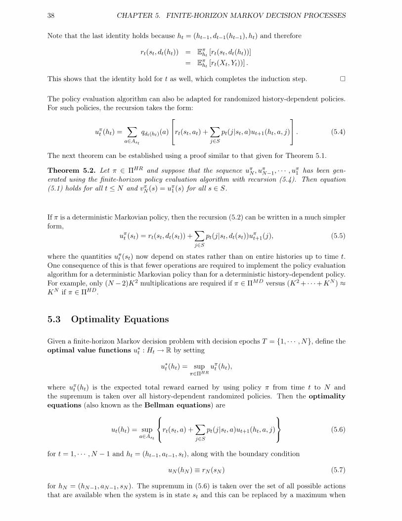
38 CHAPTER 5. FINITE-HORIZON MARKOV DECISION PROCESSES
Note that the last identity holds because ht = (ht−1, dt−1(ht−1), ht) and therefore
rt(st, dt(ht)) = Eπht [rt(st, dt(ht))]= Eπht [rt(Xt, Yt))] .
This shows that the identity hold for t as well, which completes the induction step.
The policy evaluation algorithm can also be adapted for randomized history-dependent policies.For such policies, the recursion takes the form:
uπt (ht) =∑a∈Ast
qdt(ht)(a)
rt(st, at) +∑j∈S
pt(j|st, a)ut+1(ht, a, j)
. (5.4)
The next theorem can be established using a proof similar to that given for Theorem 5.1.
Theorem 5.2. Let π ∈ ΠHR and suppose that the sequence uπN , uπN−1, · · · , uπ1 has been gen-
erated using the finite-horizon policy evaluation algorithm with recursion (5.4). Then equation(5.1) holds for all t ≤ N and vπN (s) = uπ1 (s) for all s ∈ S.
If π is a deterministic Markovian policy, then the recursion (5.2) can be written in a much simplerform,
uπt (st) = rt(st, dt(st)) +∑j∈S
pt(j|st, dt(st))uπt+1(j), (5.5)
where the quantities uπt (st) now depend on states rather than on entire histories up to time t.One consequence of this is that fewer operations are required to implement the policy evaluationalgorithm for a deterministic Markovian policy than for a deterministic history-dependent policy.For example, only (N −2)K2 multiplications are required if π ∈ ΠMD versus (K2 + · · ·+KN ) ≈KN if π ∈ ΠHD.
5.3 Optimality Equations
Given a finite-horizon Markov decision problem with decision epochs T = {1, · · · , N}, define theoptimal value functions u∗t : Ht → R by setting
u∗t (ht) = supπ∈ΠHR
uπt (ht),
where uπt (ht) is the expected total reward earned by using policy π from time t to N andthe supremum is taken over all history-dependent randomized policies. Then the optimalityequations (also known as the Bellman equations) are
ut(ht) = supa∈Ast
rt(st, a) +∑j∈S
pt(j|st, a)ut+1(ht, a, j)
(5.6)
for t = 1, · · · , N − 1 and ht = (ht−1, at−1, st), along with the boundary condition
uN (hN ) ≡ rN (sN ) (5.7)
for hN = (hN−1, aN−1, sN ). The supremum in (5.6) is taken over the set of all possible actionsthat are available when the system is in state st and this can be replaced by a maximum when

5.3. OPTIMALITY EQUATIONS 39
all of the action sets are finite. The Bellman equations are important because they can be usedto verify that a policy is optimal and can sometimes be used to identify optimal policies.
The next theorem states that solutions to the Bellman equations have certain optimality prop-erties. Part (a) implies that the solutions are the optimal value functions from period t onward,while (b) implies that the solution obtained at n = 1 is the value function for the MDP.
Theorem 5.3. Suppose that the functions u1, · · · , uN satisfy equations (5.6) - (5.7). Then
(a) ut(ht) = u∗t (ht) for all ht ∈ Ht;
(b) u1(s1) = v∗N (s1) for all s1 ∈ S.
Proof. The proof of (a) is divided into two parts, both of which rely on backwards induction ont. We begin by showing:
Claim 1: ut(ht) ≥ u∗t (ht) for all t = 1, · · · , N and all ht ∈ Ht.
To set up the induction argument, first observe that the result is true when t = N , sincecondition (5.7) guarantees that uN (hN ) = uπN (hN ) = rN (sN ) for all π ∈ ΠHR when hN =(hN−1, aN−1, sN ), which implies that uN (hN ) = u∗N (hN ). Suppose that the result is true fort = n+ 1, · · · , N (the induction hypothesis). Then, for any policy π′ = (d′1, · · · , d′N ) ∈ ΠHR, theoptimality equation for t = n and the induction hypothesis for t = n+ 1 imply that
un(hn) = supa∈Asn
rn(sn, a) +∑j∈S
pn(j|sn, a)un+1(hn, a, j)
≥ sup
a∈Asn
rn(sn, a) +∑j∈S
pn(j|sn, a)u∗n+1(hn, a, j)
≥ sup
a∈Asn
rn(sn, a) +∑j∈S
pn(j|sn, a)uπ′n+1(hn, a, j)
≥
∑a∈Asn
qd′n(hn)(a)
rn(sn, a) +∑j∈S
pn(j|sn, a)uπ′n+1(hn, a, j)
= uπ
′n (hn).
However, since π′ is arbitrary, it follows that
un(hn) ≥ supπ∈ΠHR
uπn(hn) = u∗n(hn),
which completes the induction.
We next show that:
Claim 2: For any ε > 0, there exists a deterministic policy π′ ∈ ΠHD for which
uπ′t (ht) + (N − t)ε ≥ ut(ht)
for all ht ∈ Ht and 1 ≤ t ≤ N .
Suppose that π′ = (d1, · · · , dN−1) is constructed by choosing dt(ht) = a ∈ Ast so that
rt(st, dt(ht)) +∑j∈S
pt(j|st, dt(ht))uπ′t+1(st, dt(ht), j) + ε ≥ ut(ht).
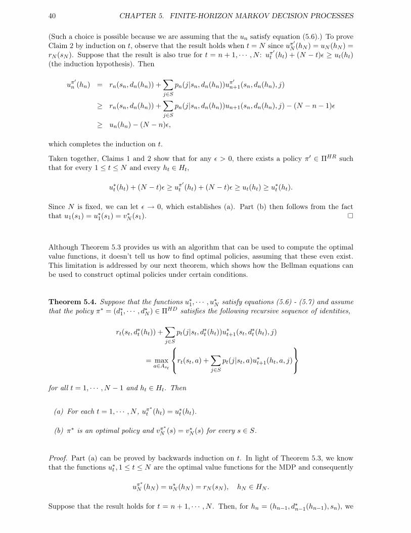
40 CHAPTER 5. FINITE-HORIZON MARKOV DECISION PROCESSES
(Such a choice is possible because we are assuming that the un satisfy equation (5.6).) To proveClaim 2 by induction on t, observe that the result holds when t = N since uπ′N (hN ) = uN (hN ) =rN (sN ). Suppose that the result is also true for t = n + 1, · · · , N : uπ′t (ht) + (N − t)ε ≥ ut(ht)(the induction hypothesis). Then
uπ′n (hn) = rn(sn, dn(hn)) +
∑j∈S
pn(j|sn, dn(hn))uπ′n+1(sn, dn(hn), j)
≥ rn(sn, dn(hn)) +∑j∈S
pn(j|sn, dn(hn))un+1(sn, dn(hn), j)− (N − n− 1)ε
≥ un(hn)− (N − n)ε,
which completes the induction on t.
Taken together, Claims 1 and 2 show that for any ε > 0, there exists a policy π′ ∈ ΠHR suchthat for every 1 ≤ t ≤ N and every ht ∈ Ht,
u∗t (ht) + (N − t)ε ≥ uπ′t (ht) + (N − t)ε ≥ ut(ht) ≥ u∗t (ht).
Since N is fixed, we can let ε → 0, which establishes (a). Part (b) then follows from the factthat u1(s1) = u∗1(s1) = v∗N (s1).
Although Theorem 5.3 provides us with an algorithm that can be used to compute the optimalvalue functions, it doesn’t tell us how to find optimal policies, assuming that these even exist.This limitation is addressed by our next theorem, which shows how the Bellman equations canbe used to construct optimal policies under certain conditions.
Theorem 5.4. Suppose that the functions u∗1, · · · , u∗N satisfy equations (5.6) - (5.7) and assumethat the policy π∗ = (d∗1, · · · , d∗N ) ∈ ΠHD satisfies the following recursive sequence of identities,
rt(st, d∗t (ht)) +∑j∈S
pt(j|st, d∗t (ht))u∗t+1(st, d∗t (ht), j)
= maxa∈Ast
rt(st, a) +∑j∈S
pt(j|st, a)u∗t+1(ht, a, j)
for all t = 1, · · · , N − 1 and ht ∈ Ht. Then
(a) For each t = 1, · · · , N , uπ∗t (ht) = u∗t (ht).
(b) π∗ is an optimal policy and vπ∗N (s) = v∗N (s) for every s ∈ S.
Proof. Part (a) can be proved by backwards induction on t. In light of Theorem 5.3, we knowthat the functions u∗t , 1 ≤ t ≤ N are the optimal value functions for the MDP and consequently
uπ∗N (hN ) = u∗N (hN ) = rN (sN ), hN ∈ HN .
Suppose that the result holds for t = n + 1, · · · , N . Then, for hn = (hn−1, d∗n−1(hn−1), sn), we
5.3. OPTIMALITY EQUATIONS 41
have
u∗n(hn) = maxa∈Asn
rn(sn, a) +∑j∈S
pn(j|sn, a)u∗n+1(hn, a, j)
= rn(sn, d∗n(hn)) +
∑j∈S
pn(j|sn, d∗n(hn))u∗n+1(hn, d∗n(hn), j)
= rn(sn, d∗n(hn)) +∑j∈S
pn(j|sn, d∗n(hn))uπ∗n+1(hn, d∗n(hn), j)
= uπ∗n (hn).
The first equality holds because the functions u∗n satisfy the Bellman equations and here we areassuming that the supremum on the right-hand side of (5.6) can be replaced by a maximum; thesecond equality holds because d∗n is assumed to be a decision rule that achieves this maximum;the third equality is a consequence of the induction hypothesis; lastly, the fourth equality is aconsequence of Theorem 5.1. This completes the induction and establishes part (a). Part (b)follows from Theorem 5.1 and Theorem 5.3 (b), along with part (a) of this theorem:
vπ∗
N (s) = uπ∗
1 (s) = u∗1(s) = v∗N (s).
It follows from this theorem that an optimal policy can be found by first solving the optimalityequations for the functions u∗1, · · · , u∗N and then recursively choosing a sequence of decision rulesd∗1, · · · , d∗N such that
d∗t (ht) ∈ arg maxa∈Ast
rt(st, a) +∑j∈S
pt(j|st, a)u∗t+1(ht, a, j)
. (5.8)
This is sometimes known as the “Principle of Optimality” , which says that a policy that isoptimal over decision epochs 1, · · · , N is also optimal when restricted to decision epochs t, · · · , N .On the other hand, optimality usually is not preserved if we truncate the time interval on theright: a policy that is optimal over decision epochs 1, · · · , N need not be optimal when restrictedto decision epochs 1, · · · , t for t < N .
Provided that the action sets are finite, there will always be at least one action that maximizesthe right-hand side of (5.8) and thus at least one optimal policy will exist under these conditions.Furthermore, if there is more than one action that maximizes the right-hand side, then there willbe multiple optimal policies (albeit with the same expected total reward). On the other hand,if the supremum is not attained in (5.6) for some t ∈ {1, · · · , N} and some ht ∈ Ht, then anoptimal policy will not exist and we must instead make do with ε-optimal policies. These canbe found using the following procedure.
Theorem 5.5. Suppose that the functions u∗1, · · · , u∗N satisfy equations (5.6) - (5.7). Givenε > 0, let πε = (dε1, · · · , dεN ) ∈ ΠHD be a policy which satisfies
rt(st, dεt(ht)) +∑j∈S
pt(j|st, dεt(ht))u∗t+1((st, dεt(ht), j)) +ε
N − 1
≥ maxa∈Ast
rt(st, a) +∑j∈S
pt(j|st, a)u∗t+1((ht, a, j))
(5.9)
for t = 1, · · · , N − 1. Then
42 CHAPTER 5. FINITE-HORIZON MARKOV DECISION PROCESSES
(a) For every t = 1, · · · , N and every ht ∈ Ht,
uπε
t (ht) + (N − t) ε
N − 1≥ u∗t (ht).
(b) πε is an ε-optimal policy and for every s ∈ S
vπε
N (s) + ε ≥ v∗N (s).
This can be proved by modifying the arguments used to establish claim (b) in Theorem 5.3.
5.4 Optimality of Deterministic Markov Policies
Because deterministic Markov policies are generally easier to implement and require less com-putational effort than randomized history-dependent policies, it is important to know when theexistence of an optimal or ε-optimal policy of this type is guaranteed. In this section, we willshow that if an optimal policy exists for a finite-horizon MDP, then there is an optimal policythat is deterministic and Markovian. Our first theorem summarizes some properties of the de-terministic history-dependent policies that are constructed in the proofs of Theorems 5.3 - 5.5.
Theorem 5.6. Existence of deterministic history-dependent policies.
(a) For any ε > 0, there exists an ε-optimal policy which is deterministic and history-dependent.Furthermore, any policy π ∈ ΠHD which satisfies the inequalities given in (5.9) is ε-optimal.
(b) Let (u∗t , 1 ≤ t ≤ N) satisfy the optimal value equations (5.6) - (5.7) and suppose that foreach t and each st ∈ S, there exists an a′ ∈ Ast such that
rt(st, a′) +∑j∈S
pt(j|st, a′)u∗t+1(ht, a′, j)
= supa∈Ast
rt(st, a) +∑j∈S
pt(j|st, a)u∗t+1(ht, at, j)
(5.10)
for all histories ht = (st−1, at−1, st) ∈ Ht. Then there exists a deterministic history-dependent policy which is optimal.
Our next theorem strengthens these results by asserting the existence of deterministic Markovpolicies which are ε-optimal or optimal.
Theorem 5.7. Let (u∗t , 1 ≤ t ≤ N) satisfy the optimal value equations (5.6) - (5.7). Then
(a) For each t = 1, · · · , N , u∗t (ht) depends on ht only through st.
(b) For any ε > 0, there exists an ε-optimal policy which is deterministic and Markov.
(c) If there exists an a′ ∈ Ast such that equation (5.10) holds for each st ∈ S and t =1, 2, · · · , N − 1, then there exists an optimal policy which is deterministic and Markov.
5.4. OPTIMALITY OF DETERMINISTIC MARKOV POLICIES 43
Proof. Part (a) can be proved by backwards induction on t. Since u∗N (hN ) = rN (sN ), the resultis clearly true for t = N . Thus, let the induction hypothesis be that the result is true fort = n+ 1, · · · , N . Then, according to equation (5.6),
u∗n(hn) = supa∈Asn
rn(sn, a) +∑j∈S
pn(j|sn, a)un+1((hn, a, j))
= sup
a∈Asn
rn(sn, a) +∑j∈S
pn(j|sn, a)un+1(j)
,
where the second equality follows from the induction hypothesis for t = n+ 1. This shows thatu∗n(hn) depends on hn only through sn, which completes the induction.
To prove part (b), choose ε > 0 and let πε = (dε1, · · · , dεN−1) ∈ ΠMD be any policy which satisfiesthe inequalities
rt(st, dεt(st)) +∑j∈S
pt(j|st, dεt(st))uεt+1(j) +ε
N − 1
≥ supa∈Ast
rt(st, a) +∑j∈S
pt(j|st, a)uεt+1(j)
,
Then πε satisfies the conditions of Theorem 5.6 (a) and thus is ε-optimal.
Lastly, part (c) follows because we can construct a policy π∗ = (d∗1, · · · , d∗N−1) ∈ ΠMD such that
rt(st, d∗t (st)) +∑j∈S
pt(j|st, d∗t (st))u∗t+1(j)
= supa∈Ast
rt(st, a) +∑j∈S
pt(j|st, a)u∗t+1(j)
,
and then Theorem 5.4 (b) implies that π∗ is an optimal policy.
It follows from Theorem 5.7 that
v∗N (s) = supπ∈ΠHR
vπN (s) = supπ∈ΠMD
vπN (s), s ∈ S,
and thus it suffices to restrict attention to deterministic Markov policies when studying finite-horizon Markov decision problems with the total expected reward criterion.
Although not every Markov decision problem has an optimal policy (of any type), there areseveral simple conditions that guarantee the existence of at least one optimal policy. We beginwith a definition.
Definition 5.1. Suppose that f : D → [−∞,∞] is a real-valued function defined on a domainD ⊂ Rn. Then f is said to be upper semicontinuous if
lim supxn→x
f(xn) ≤ f(x)
for any sequence (xn;n ≥ 1) converging to x. Similarly, f is said to be lower semicontinuousif
lim infxn→x
f(xn) ≥ f(x)
for any sequence (xn;n ≥ 1) converging to x.

44 CHAPTER 5. FINITE-HORIZON MARKOV DECISION PROCESSES
Some important properties of upper and lower semicontinuous functions are listed below.
1. f is continuous if and only if it is both upper and lower semicontinuous.
2. f is upper semicontinuous if and only if −f is lower semicontinuous.
3. If f is upper semicontinuous and C ⊂ D is a compact set, then f achieves its maximumon C, i.e., there is a point x∗ ∈ C such that
f(x∗) = supx∈C
f(x).
Theorem 5.8. Assume that the state space S is countable and that one of the following threesets of criteria are satisfied:
(a) As is finite for each s ∈ S, or
(b) As is compact for each s ∈ S; rt(s, a) is a continuous function of a for all t ∈ T and s ∈ S,and there exists a constant M < ∞ such that |rt(s, a)| ≤ M for all t ∈ T , s ∈ S, anda ∈ As; and pt(j|s, a) is continuous in a for all s, j ∈ S and t ∈ T , or
(c) As is compact for each s ∈ S; rt(s, a) is upper semicontinuous in a for all t ∈ T and s ∈ S,and there exists a constant M < ∞ such that |rt(s, a)| ≤ M for all t ∈ T , s ∈ S anda ∈ As; and pt(j|s, a) is lower semicontinuous in a for all s, j ∈ S and t ∈ T .
Then there exists a deterministic Markovian policy which is optimal.
Proof. According to Theorem 5.7 (c), it suffices to show that for every s ∈ S and t ∈ T , thereexists an action a′ ∈ As such that
rt(st, a′) +∑j∈S
pt(j|st, a′)u∗t+1(j)
= supa∈Ast
rt(st, a) +∑j∈S
pt(j|st, a)u∗t+1(j)
.
This is clearly true if each action set As is finite. Alternatively, if the conditions in (b) are true,then it suffices to show that the functions
Ψt(s, a) ≡ rt(s, a) +∑j∈S
pt(j|s, a)u∗t+1(j)
are continuous in a for all t ∈ T and s ∈ S, since we know that the sets As are compact and anycontinuous function achieves its maximum on a compact set. However, since the rewards rt(s, a)are assumed to be continuous in a, it suffices to show that the sum∑
j∈Spt(j|s, a)u∗t+1(j)
is a continuous function of a for all t ∈ T and s ∈ S. To this end, we first show that theconditions in (b) imply that the functions u∗t are bounded on S. Indeed, since the optimal valuefunctions satisfy the recursive equations,
u∗t (s) = supa∈As
rt(s, a) +∑j∈S
pt(j|s, a)u∗t+1(j)
,
5.4. OPTIMALITY OF DETERMINISTIC MARKOV POLICIES 45
it follows that|u∗t (s)| ≤M + sup
s′∈S|u∗t+1(s′)|,
for all s ∈ S, which implies that
sups∈S|u∗t (s)| ≤M + sup
s∈S|u∗t+1(s)|
for all t = 1, · · · , N . However, since
sups∈S|u∗N (s)| = sup
s∈S|rN (s)| ≤M,
a simple induction argument shows that
sups∈S|u∗t (s)| ≤ NM
for t = 1, · · · , N , and so the optimal value functions are bounded as claimed above.
To complete the argument, let ε > 0 be given and suppose that (an : n ≥ 0) is a sequence inAs which converges to a∞. Since the functions pt(j|s, a) are continuous in a for all t ∈ T ands, j ∈ S, we know that
pt(j|s, a∞) = limn→∞
pt(j|s, an). (5.11)
Furthermore, since for each t ∈ T , s ∈ S and a ∈ As, we know that pt(·|s, a) is a probabilitydistribution on S, we can choose a finite subset K ≡ K(t, s, a) = {j1, · · · , jM} ⊂ S such that∑
j∈Kpt(j|s, a) > 1− ε.
For each element ji ∈ K, use (5.11) to choose Ni large enough that for all n ≥ Ni, we have
|pt(ji|s, a)− pt(ji|s, an)| < ε
M.
Summing over the elements in K and using the triangle inequality gives∣∣∣∣∣∣1−∑j∈K
pt(j|s, an)
∣∣∣∣∣∣ ≤∣∣∣∣∣∣1−
∑j∈K
pt(j|s, a) +∑j∈K
pt(j|s, a)−∑j∈K
pt(j|s, an)
∣∣∣∣∣∣≤ ε+
∑j∈K|pt(j|s, a)− pt(j|s, an)|
≤ ε+M · εM
= 2ε
for all n ≥ N ≡ max{N1, · · · , NM} <∞. Thus∑j∈Kc
pt(j|s, an) ≤ 2ε
for all n ≥ N and consequently∣∣∣∣∣∣∑j∈Kc
pt(j|s, an)u∗t+1(j)
∣∣∣∣∣∣ ≤∑j∈Kc
pt(j|s, an)∣∣u∗t+1(j)
∣∣ ≤ 2NMε

46 CHAPTER 5. FINITE-HORIZON MARKOV DECISION PROCESSES
for all such n (including n =∞). Finally, if n ≥ N , then these results give∣∣∣∣∣∣∑j∈S
pt(j|s, a)u∗t+1(j)−∑j∈S
pt(j|s, an)u∗t+1(j)
∣∣∣∣∣∣ ≤∑j∈S
∣∣pt(j|s, a)u∗t+1(j)− pt(j|s, an)u∗t+1(j)∣∣
=∑j∈K
∣∣pt(j|s, a)u∗t+1(j)− pt(j|s, an)u∗t+1(j)∣∣+
∑j∈Kc
∣∣pt(j|s, a)u∗t+1(j)− pt(j|s, an)u∗t+1(j)∣∣
≤∑j∈K|pt(j|s, a)− pt(j|s, an)|
∣∣u∗t+1(j)∣∣+
∑j∈Kc
∣∣pt(j|s, a)u∗t+1(j)∣∣+
∑j∈Kc
∣∣pt(j|s, an)u∗t+1(j)∣∣
≤ NMε+ 2NMε+ 2NMε
= 5NMε.
However, since N and M are fixed and ε > 0 can be made arbitrarily small, it follows that thedifference ∣∣∣∣∣∣
∑j∈S
pt(j|s, a)u∗t+1(j)−∑j∈S
pt(j|s, an)u∗t+1(j)
∣∣∣∣∣∣→ 0
as n tends to infinity. This establishes that the sum appearing in Ψt(s, a) is continuous in a andtherefore so is Ψt(s, a) itself, which is what we needed to show.
For the proof that (c) is sufficient to guarantee the existence of an optimal policy, see p. 91 andappendix B of Puterman (2005).
5.5 The Backward Induction Algorithm
In the last section, we showed that a finite-horizon MDP is guaranteed to have at least oneoptimal policy that is both Markovian and deterministic if the optimality equations (5.10) canbe solved for every t = 1, · · · , N − 1 and s ∈ S. In this case, all such optimal policies can befound with the help of the backward induction algorithm, which consists of the followingsteps:
1. Set t = N and letu∗N (s) = rN (s) for all s ∈ S.
2. Substitute t− 1 for t and let
u∗t (s) = maxa∈As
rt(s, a) +∑j∈S
pt(j|s, a)u∗t+1(j)
(5.12)
A∗s,t = arg maxa∈As
rt(s, a) +∑j∈S
pt(j|s, a)u∗t+1(j)
. (5.13)
3. Stop if t = 1. Otherwise return to step 2.

5.6. EXAMPLES 47
It then follows that vN (s) = u∗1(s) is the value of the Markov decision problem and that anypolicy π∗ = (d∗1, · · · , d∗N−1) ∈ ΠMD with the property that
d∗t (s) ∈ A∗s,t (5.14)
for every t = 1, · · · , N − 1 and s ∈ S is optimal, i.e., vπ∗N = v∗N (s) for every s ∈ S. Conversely,if π∗ ∈ ΠMD is an optimal policy for the MDP, then π∗ satisfies condition (5.14). Notice thatthere will be more than one optimal policy if and only if at least one of the sets A∗s,t containsmore than one element.
If |S| = K and |As| = L for each s ∈ S, then full implementation of the backward inductionalgorithm will require at most (N − 1)LK2 multiplications and an equivalent number of eval-uations of the transition probabilities. This assumes that every transition probability pt(j|s, a)is positive. If, instead, most transitions are forbidden, i.e., if pt(j|s, a) = 0 for most s, j ∈ S,then much less effort will be needed. Likewise, if the sets As are subsets of Rn, then it may bepossible to use analytical or numerical tools to solve the maximization problem in (5.12).
5.6 Examples
5.6.1 The Secretary Problem
Recall the problem: N candidates are interviewed sequentially, in random order, and at theconclusion of each interview we can either offer the position to that candidate or reject them andmove on to the next. The aim is to maximize the probability that we offer the position to thebest candidate, assuming that we can discern the relative ranks of the candidates interviewedbut not their absolute ranks.
Let u∗t (1) be the maximum probability that we choose the best candidate given that the t’thcandidate is the best interviewed so far and let u∗t (0) be the maximum probability that we choosethe best candidate given that the t’th candidate is not the best one interviewed so far. Theseare the optimal value functions for this problem and thus they satisfy the following recursions:
u∗N (1) = 1, u∗N (0) = 0, u∗N (∆) = 0,
and, for t = 1, · · · , N − 1,
u∗t (0) = max{gt(0) + u∗t+1(∆), 0 + pt(1|0)u∗t+1(1) + pt(0|0)u∗t+1(0)
}= max
{0,
1t+ 1
u∗t+1(1) +t
t+ 1u∗t+1(0)
}=
1t+ 1
u∗t+1(1) +t
t+ 1u∗t+1(0),
u∗t (1) = max{gt(1) + u∗t+1(∆), 0 + pt(1|1)u∗t+1(1) + pt(0|1)u∗t+1(0)
}= max
{t
N,
1t+ 1
u∗t+1(1) +t
t+ 1u∗t+1(0)
}= max
{t
N, u∗t (0)
},
u∗t (∆) = u∗t+1(∆) = 0.
From these equations, we see that an optimal policy for this problem can be formulated asfollows. In state 0, the optimal action is always to continue (if t < N), as we know that thecurrent candidate is not best overall. In contrast, in state 1, the optimal action is to continue ifu∗t (0) > t and to stop if u∗t (0) < t/N ; if u∗t (0) = t/N , then either action is optimal.
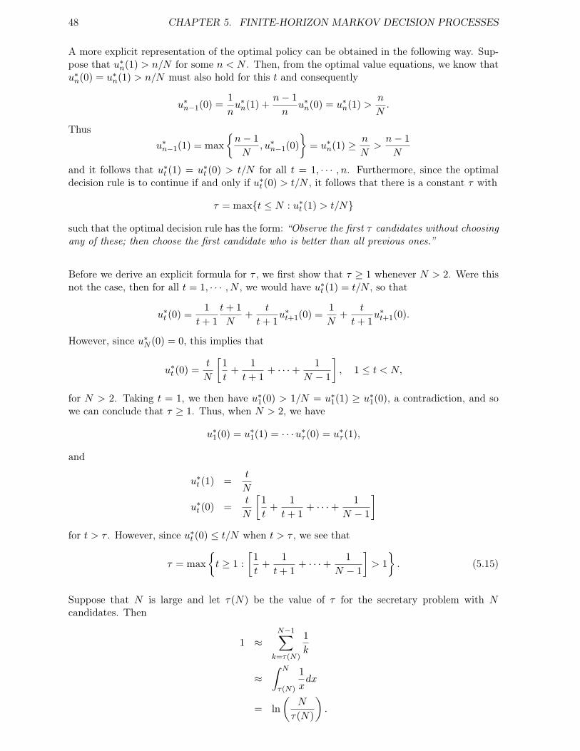
48 CHAPTER 5. FINITE-HORIZON MARKOV DECISION PROCESSES
A more explicit representation of the optimal policy can be obtained in the following way. Sup-pose that u∗n(1) > n/N for some n < N . Then, from the optimal value equations, we know thatu∗n(0) = u∗n(1) > n/N must also hold for this t and consequently
u∗n−1(0) =1nu∗n(1) +
n− 1n
u∗n(0) = u∗n(1) >n
N.
Thusu∗n−1(1) = max
{n− 1N
, u∗n−1(0)}
= u∗n(1) ≥ n
N>n− 1N
and it follows that u∗t (1) = u∗t (0) > t/N for all t = 1, · · · , n. Furthermore, since the optimaldecision rule is to continue if and only if u∗t (0) > t/N , it follows that there is a constant τ with
τ = max{t ≤ N : u∗t (1) > t/N}
such that the optimal decision rule has the form: “Observe the first τ candidates without choosingany of these; then choose the first candidate who is better than all previous ones.”
Before we derive an explicit formula for τ , we first show that τ ≥ 1 whenever N > 2. Were thisnot the case, then for all t = 1, · · · , N , we would have u∗t (1) = t/N , so that
u∗t (0) =1
t+ 1t+ 1N
+t
t+ 1u∗t+1(0) =
1N
+t
t+ 1u∗t+1(0).
However, since u∗N (0) = 0, this implies that
u∗t (0) =t
N
[1t
+1
t+ 1+ · · ·+ 1
N − 1
], 1 ≤ t < N,
for N > 2. Taking t = 1, we then have u∗1(0) > 1/N = u∗1(1) ≥ u∗1(0), a contradiction, and sowe can conclude that τ ≥ 1. Thus, when N > 2, we have
u∗1(0) = u∗1(1) = · · ·u∗τ (0) = u∗τ (1),
and
u∗t (1) =t
N
u∗t (0) =t
N
[1t
+1
t+ 1+ · · ·+ 1
N − 1
]for t > τ . However, since u∗t (0) ≤ t/N when t > τ , we see that
τ = max{t ≥ 1 :
[1t
+1
t+ 1+ · · ·+ 1
N − 1
]> 1}. (5.15)
Suppose that N is large and let τ(N) be the value of τ for the secretary problem with Ncandidates. Then
1 ≈N−1∑
k=τ(N)
1k
≈∫ N
τ(N)
1xdx
= ln(
N
τ(N)
).

5.7. MONOTONE POLICIES 49
In fact, these approximations can be replaced by identities if we take the limit as N →∞, whichshows that
limN→∞
τ(N)N
= e−1
and alsolimN→∞
u∗1(0) = limN→∞
u∗1(1) = limN→∞
u∗τ(N)(0) = limN→∞
τ(N)N
= e−1.
Thus, when N is sufficiently large, the optimal policy is to observe the first N/e candidates andthen then choose the next one to come along with the highest relative rank, in which case theprobability that that candidate is the best one overall is approximately 1/e ≈ 0.368.
5.7 Monotone Policies
Definition 5.2. Suppose that the state space S and all of the action sets As for a finite-horizonMarkov decision problem are ordered sets, and let π = (d1, · · · , dN−1) be a deterministic Markovpolicy for this problem.
(a) π is said to be non-decreasing if for each t = 1, · · · , N−1 and any pair of states s1, s2 ∈ Swith s1 < s2, it is true that dt(s1) ≤ dt(s2).
(b) π is said to be non-increasing if for each t = 1, · · · , N−1 and any pair of states s1, s2 ∈ Swith s1 < s2, it is true that dt(s1) ≥ dt(s2).
(c) π is said to be monotone if it is either non-decreasing or non-increasing.
Monotone policies are of special interest because they are sometimes easier to compute and easierto implement. For example, control limit policies, which have decision rules of the form
dt(s) =
{a1 if s < s∗ta2 if s ≥ s∗t ,
can be interpreted as monotone policies if the set {a1, a2} is equipped with an ordering such thata1 < a2, say.
In this section, we will describe some conditions on Markov decision problems which guaranteethe existence of optimal policies which are monotone. We will then see how the backward in-duction algorithm can be modified to efficiently search for such policies. However, we begin byintroducing a special class of bivariate functions which have been found to be useful in a varietyof problems involving dynamic programming.
Definition 5.3. Suppose that X and Y are partially-ordered sets. A real-valued function g :X × Y → R is said to be superadditive if for all x− ≤ x+ in X and all y− ≤ y+ in Y ,
g(x−, y−) + g(x+, y+) ≥ g(x−, y+) + g(x+, y−). (5.16)
Alternatively, g is said to be subadditive if the reverse inequality holds.
Superadditive (subadditive) functions are sometimes said to be supermodular (submodular),while (5.16) is sometimes called the quadrangle inequality. Any separable function h(x, y) =f(x) + g(y) is both super- and subadditive, and clearly a function h(x, y) is superadditive if

50 CHAPTER 5. FINITE-HORIZON MARKOV DECISION PROCESSES
and only if the function −h(x, y) is subadditive. Furthermore, if X,Y ⊂ R and g is a twicecontinuously differentiable function with
∂2g(x, y)∂x∂y
≥ 0
then g is superadditive.
We will need two technical lemmas which we state without proof (see Section 4.7 in Puterman(2005)). Our first lemma establishes an important relationship between superadditive functionsand nondecreasing functions.
Lemma 5.1. Suppose that g : X×Y → R is superadditive and that for each x ∈ X the maximummaxy g(x, y) is realized. Then the function
f(x) ≡ max{y′ ∈ arg maxy∈Y
g(x, y)}
is monotone nondecreasing in x.
Lemma 5.2. Suppose that (pn;n ≥ 0) and (p′n;n ≥ 0) are sequences of non-negative real numberssuch that the inequality
∞∑j=k
pj ≤∞∑j=k
p′j
holds for every k ≥ 1, with equality when k = 0. If (vj ; j ≥ 0) is a nondecreasing sequence of realnumbers (not necessarily non-negative), then
∞∑j=0
pjvj ≤∞∑j=0
p′jvj .
In particular, if X and Y are non-negative integer-valued random variables with pj = P(X = j)and p′j = P(Y = j), then the theorem asserts that if Y is stochastically greater than X, thenE[f(X)] ≤ E[f(Y )] for any nondecreasing function f : N→ R.
Before we can prove that monotone optimal policies exist under certain general conditions, wefirst need to investigate the monotonicity properties of the optimal value functions. For the restof this section we will assume that S = N, that As = A′ for all s ∈ S and that the maximum
maxa∈A′
rt(s, a) +∞∑j=0
p(j|s, a)u(j)
is attained for all s ∈ S, t ∈ T and all monotone functions u : S → R. We will also let
qt(k|s, a) ≡∞∑j=k
pt(j|s, a)
denote the probability that the system moves to a state j ≥ k when it was in state s at time tand action a was selected.
Proposition 5.1. Let (u∗1, · · · , u∗N ) be the optimal value functions for a MDP and assume that
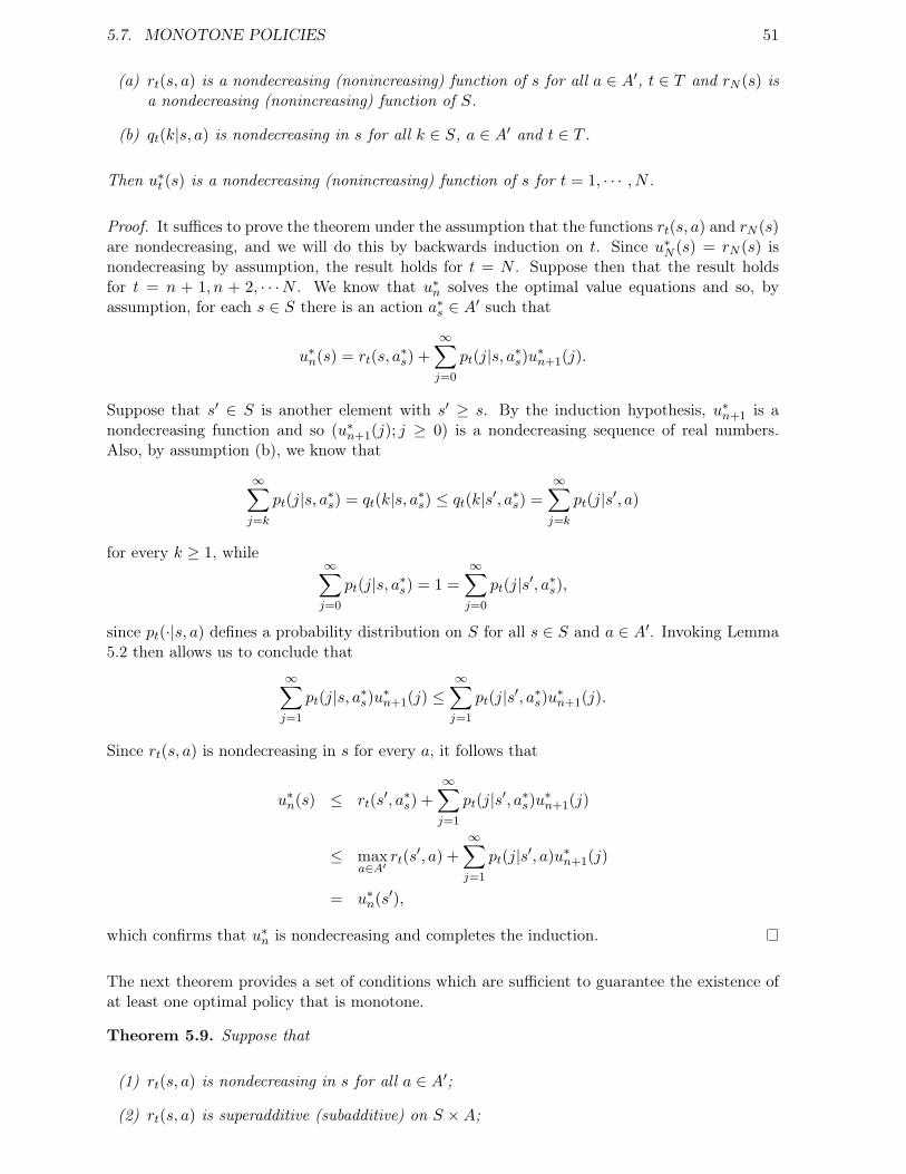
5.7. MONOTONE POLICIES 51
(a) rt(s, a) is a nondecreasing (nonincreasing) function of s for all a ∈ A′, t ∈ T and rN (s) isa nondecreasing (nonincreasing) function of S.
(b) qt(k|s, a) is nondecreasing in s for all k ∈ S, a ∈ A′ and t ∈ T .
Then u∗t (s) is a nondecreasing (nonincreasing) function of s for t = 1, · · · , N .
Proof. It suffices to prove the theorem under the assumption that the functions rt(s, a) and rN (s)are nondecreasing, and we will do this by backwards induction on t. Since u∗N (s) = rN (s) isnondecreasing by assumption, the result holds for t = N . Suppose then that the result holdsfor t = n + 1, n + 2, · · ·N . We know that u∗n solves the optimal value equations and so, byassumption, for each s ∈ S there is an action a∗s ∈ A′ such that
u∗n(s) = rt(s, a∗s) +∞∑j=0
pt(j|s, a∗s)u∗n+1(j).
Suppose that s′ ∈ S is another element with s′ ≥ s. By the induction hypothesis, u∗n+1 is anondecreasing function and so (u∗n+1(j); j ≥ 0) is a nondecreasing sequence of real numbers.Also, by assumption (b), we know that
∞∑j=k
pt(j|s, a∗s) = qt(k|s, a∗s) ≤ qt(k|s′, a∗s) =∞∑j=k
pt(j|s′, a)
for every k ≥ 1, while∞∑j=0
pt(j|s, a∗s) = 1 =∞∑j=0
pt(j|s′, a∗s),
since pt(·|s, a) defines a probability distribution on S for all s ∈ S and a ∈ A′. Invoking Lemma5.2 then allows us to conclude that
∞∑j=1
pt(j|s, a∗s)u∗n+1(j) ≤∞∑j=1
pt(j|s′, a∗s)u∗n+1(j).
Since rt(s, a) is nondecreasing in s for every a, it follows that
u∗n(s) ≤ rt(s′, a∗s) +∞∑j=1
pt(j|s′, a∗s)u∗n+1(j)
≤ maxa∈A′
rt(s′, a) +∞∑j=1
pt(j|s′, a)u∗n+1(j)
= u∗n(s′),
which confirms that u∗n is nondecreasing and completes the induction.
The next theorem provides a set of conditions which are sufficient to guarantee the existence ofat least one optimal policy that is monotone.
Theorem 5.9. Suppose that
(1) rt(s, a) is nondecreasing in s for all a ∈ A′;
(2) rt(s, a) is superadditive (subadditive) on S ×A;

52 CHAPTER 5. FINITE-HORIZON MARKOV DECISION PROCESSES
(3) qt(k|s, a) is nondecreasing in s for all k ∈ S and a ∈ A′;
(4) qt(k|s, a) is superadditive (subadditive) on S ×A for every k ∈ S;
(5) rN (s) is a nondecreasing in s.
Then there exist optimal decision rules d∗t (s) which are nondecreasing (nonincreasing) in s fort = 1, · · · , N − 1.
Proof. The assumption that qt is superadditive implies that for every k ≥ 1
∞∑j=k
[pt(j|s−, a−) + pt(j|s+, a+)
]≥∞∑j=k
[pt(j|s−, a+) + pt(j|s+, a−)
]for all s− ≤ s+, a− ≤ a+. However, since Proposition 5.1 implies that the optimal value functionsu∗t (s) are nondecreasing, we can use Lemma 5.2 to conclude that
∞∑j=k
[pt(j|s−, a−) + pt(j|s+, a+)
]ut(j) ≥
∞∑j=k
[pt(j|s−, a+) + pt(j|s+, a−)
]ut(j),
which shows that the functions∑
j≥0 pt(j|s, a)ut(j) are superadditive for every t = 1, · · · , N −1.By assumption, the rewards rt(s, a) are superadditive and thus so are the functions
wt(s, a) ≡ rt(s, a) +∞∑j=0
pt(j|s, a)u∗t (j)
(since sums of superadditive functions are superadditive). It then follows from Lemma 5.1 thatif we define decision rules dt(s) by setting
dt(s) = max{a∗ ∈ arg max
Aswt(s, a)
},
then dt is a nondecreasing function and so the policy π = (d1, · · · , dN−1) is optimal and mono-tone.
Example 5.1. A Price Determination Model. Suppose that a manager wishes to determineoptimal price levels based on current sales with the goal of maximizing revenue over some fixedperiod. This problem can be formulated as a Markov decision process by taking
• Decision epochs: T = {1, 2, · · · , N}.
• States: S = N, where st is the number of products sold in the previous month.
• Actions: As = A′ = [aL, aU ], where aL and aM are the minimum and maximum price levelsand at = a is the price assigned to the product during the t’th decision epoch.
• Rewards: let rt(s, a) denote the expected revenue in month t if the previous month’s saleswere s and the price is set to a in the current month. For simplicity, assume that theproduct has a limited shelf life and that rN (s) = 0 for all s ≥ 0.
• Transition probabilities: let pt(j|s, a) be the probability that j units are sold in month t atprice a given that s units were sold in the previous month.

5.7. MONOTONE POLICIES 53
If we assume that rt(s, a) and pt(s, a) are continuous functions of a, then Theorem 5.8 guar-antees the existence of an optimal policy which is deterministic and Markov. Furthermore, ifthe conditions of Theorem 5.9 are satisfied, then we can conclude that there is an optimal policywhich is nondecreasing in s, i.e., the greater the level of sales in the previous month, the higherthe price should be in the present month. Since rN (s) ≡ 0, condition (5) is trivially satisfied andso we need only consider the first four conditions.
(1) To stipulate that rt(s, a) is a nondecreasing function of s means that for each price a, theexpected revenue in the current month will be an increasing function of the previous month’ssales.
(2) Superadditivity of rt(s, a) requires that for s+ ≥ s− and a+ ≥ a−,
rt(s+, a+)− rt(s+, a−) ≥ rt(s−, a+)− rt(s−, a−),
which says that the effect of increasing the price on revenue is greater when the previousmonth’s sales have been greater.
(3) To stipulate that qt(k|s, a) is nondecreasing means that sales one month ahead are stochas-tically increasing with respect to current sales.
(4) Superadditivity of qt(j|s, a) requires that for every k ≥ 0,
qt(k|s+, a+)− qt(k|s+, a−) ≥ qt(k|s−, a+)− qt(k|s−, a−),
which says that the incremental effect of a price increase on the probability that sales exceeda fixed level is greater if current sales are greater.
The backward induction algorithm of section 5.5 can be simplified when it is known that a mono-tone optimal policy exists. Assuming that this is true and that the state space S = {0, 1, · · · ,M}is finite, the Monotone Backward Induction Algorithm consists of the following steps:
1. Set t = N andu∗N (s) = rN (s) for all s ∈ S.
2. Substitute t− 1 for t, set s = 1 and A′1 = A′, and
u∗t (s) = maxa∈A′s
rt(s, a) +∑j∈S
pt(j|s, a)u∗t+1(j)
(5.17)
A∗s,t = arg maxa∈A′s
rt(s, a) +∑j∈S
pt(j|s, a)u∗t+1(j)
. (5.18)
3. If s = M , go to Step 4. Otherwise, set
A′s+1 ={a ∈ A′ : a ≥ [maxAs,t]
}4. Stop if t = 1. Otherwise return to step 2.
A monotone optimal policy can then be found by forming decision rules which select actionsfrom A∗s,t in state s at decision epoch t. One advantage that this approach has over the standardbackward induction algorithm is that the maximizations performed at each epoch t are carriedout over sets A′s which can shrink as s increases.

Chapter 6
Infinite-Horizon Models: Foundations
6.1 Assumptions and Definitions
Our focus in this chapter will be on infinite-horizon Markov decision processes with stationaryrewards and transition probabilities. Throughout we will assume that the set of decision epochs isT = {1, 2, · · · } and that the reward functions and transition probabilities do not vary over time,i.e., for every t ∈ T we have rt(s, a) = r(s, a) and pt(j|s, a) = p(j|s, a). We will be especiallyinterested in stationary policies, which which we denote π = d∞ = (d, d, · · · ), meaning that thesame decision rule d is used in every decision epoch.
As before, let Xt denote the random state occupied by the process at time t, let Yt denote theaction taken in this decision epoch, and let Zt be the history of the process up to time t. Ifπ = (d1, d2, · · · ) is a deterministic policy, then Yt will be a deterministic function either of thesystem state at time t, i.e., Yt = dt(Xt), or of the process history up to time t, i.e., Yt = dt(Zt),depending on whether π is Markov or history-dependent. If, instead, π is a randomized policy,then Yt is chosen randomly according to a probability distribution qdt on the set of actions andthis distribution will take the form
P(Yt = a) =
qdt(Xt)(a) if π is Markov
qdt(Zt)(a) if π is history-dependent.
Lastly, if π is Markov, then (Xt, r(Xt, Yt); t ≥ 1) is called a Markov reward process.
There are several performance metrics that can be used to assign a value to a policy π ∈ ΠHR
which depend on the initial state of the system. The first of these is the expected total rewardof π, which is defined to be
vπ(s) ≡ limN→∞
Eπs
[N∑t=1
r(Xt, Yt)
]= lim
N→∞vπN+1(s), (6.1)
where, as before, vπN+1(s) is the total expected reward in a model restricted to N decision epochsand terminal reward 0. In general, this limit need not exist or it may exist but be equal to ±∞.Moreover, even when the limit exists, it need not be the case that the limit and expectation canbe interchanged, i.e., we cannot simply assume that
limN→∞
Eπs
[N∑t=1
r(Xt, Yt)
]= Eπs
[ ∞∑t=1
r(Xt, Yt)
], (6.2)
although we will give some conditions under which this identity does hold. Because of thesecomplications, the total expected value is not always suitable for infinite-horizon MDPs.
54

6.1. ASSUMPTIONS AND DEFINITIONS 55
An alternative performance metric is the expected total discounted reward of π, which isdefined to be
vπλ(s) ≡ limN→∞
Eπs
[N∑t=1
λt−1r(Xt, Yt)
], (6.3)
where λ ∈ [0, 1) is the discount rate. Notice that the limit is guaranteed to exist if the absolutevalue of the reward function is uniformly bounded, i.e., if |r(s, a)| ≤M for all s ∈ S and a ∈ As,in which case the total expected discounted reward is also uniformly bounded: vπλ(s) ≤M/(1−λ).Furthermore, if equality does hold in (6.2), then we also have
vπ(s) = limλ↑1
vπλ(s).
Our last performance metric is the average reward (average gain) of π, which is defined by
gπ(s) ≡ limN→∞
1N
Eπs
[N∑t=1
r(Xt, Yt)
]= lim
N→∞
1NvπN+1(s), (6.4)
provided that the limit exists. If the limit in (6.4) does not exist, then we can define the lim infaverage reward gπ− and the lim sup average reward gpi+ by
gπ−(s) ≡ lim infN→∞
1NvπN+1(s), gπ+(s) ≡ lim sup
N→∞
1NvπN+1(s).
These are guaranteed to exist (although they could be infinite) and they provide upper and lowerbounds on the average reward attainable by policy π.
Example 6.1. (Puterman, Example 5.1.2) Let S = {1, 2, · · · } and As = {a} for all s ≥ 1, i.e.,there is a single action available in all states, and suppose that the transition probabilities areequal to
pt(j|s, a) =
{1 if j = s+ 10 otherwise,
so that the state increases by 1 at each time point, and that the rewards are equal to
r(s, a) = (−1)s+1s.
Since there is only action available in each state, it follows that there is only one policy π = d∞
where d(s) = a for all s ≥ 1. Furthermore, a simple calculation shows that the total expectedreward up to time N when the initial state is s1 = 1 is equal to
vπN =
{k if N = 2k is even−k if N = 2k + 1 is odd
and so the total expected rewardvπ(1) ≡ lim
N→∞vπN (1)
does not exist. Similarly, the gain gπ(1) does not exist because
gπ+(s) = lim supN→∞
1NvπN+1(s) =
12
andgπ−(s) = lim inf
N→∞
1NvπN+1(s) = −1
2.

56 CHAPTER 6. INFINITE-HORIZON MODELS: FOUNDATIONS
On the other hand, the expected total discounted reward for this policy does exist and is finite forevery λ ∈ [0, 1) since
vπλ(1) = limN→∞
N∑t=1
λt−1(−1)t−1t = − limN→∞
d
dλ
(N∑t=1
(−λ)t)
= − limN→∞
d
dλ
(−λ1− (−λ)N
1 + λ
)= lim
N→∞
(1− (−λ)N
1 + λ+ λ
(1 + λ)N(−λ)N−1 − (1− (−λ)N
(1 + λ)2
)=
11 + λ
− λ
(1 + λ)2=
1(1 + λ)2
.
Also, notice that the limit as λ increases to 1 of the expected total discounted reward exists andis finite,
limλ↑1
vπλ(1) =14,
even though the total expected reward is not defined in this case.
6.2 The Expected Total Reward Criterion
Although we saw in the previous section that the limit that defines the total expected reward,
vπ(s) = limN→∞
vπN (s), (6.5)
does not always exist, there are relatively general conditions on a Markov decision problem whichsuffice to guarantee convergence of this sequence within the extended real numbers [−∞,∞].Define the quantities
vπ+(s) ≡ Eπs
[ ∞∑t=1
r+(Xt, Yt)
]and
vπ−(s) ≡ Eπs
[ ∞∑t=1
r−(Xt, Yt)
],
where r+(s, a) ≡ max{r(s, a), 0} and r−(s, a) ≡ max{−r(s, a), 0} are the positive and negativeparts of r(s, a), respectively. Since r+(s, a) and r−(s, a) are both non-negative, the quantitiesvπ+(s) and vπ−(s) are guaranteed to exist, although they could be equal to ∞.
For the total expected reward to be well-defined, we need to rule out the possibility that thesequence (vπN (s);N ≥ 1) assumes arbitrarily large positive and arbitrarily large negative values.To this end, we will consider Markov decision processes that satisfy the following condition.Suppose that for every policy π ∈ ΠHR and every s ∈ S, at least one of the the quantities vπ+(s)and vπ−(s) is finite. Then the limit (6.5) exists and the total expected reward is equal to
vπ(s) = vπ+(s)− vπ−(s). (6.6)
Although this condition excludes certain kinds of Markov decision processes, it is sufficientlygeneral that there are several classes of models encountered in practice which do satisfy it. Wewill introduce three such classes in the following definition.
Definition 6.1. Suppose that {N, S,As, r(s, a), p(j|s, a)} is an infinite horizon Markov decisionprocess with stationary rewards and transition probabilities.
(i) We will say that the process belongs to the class of positive bounded models if for eachs ∈ S, there exists an a ∈ As such that r(s, a) ≥ 0 and vπ+(s) is finite for all policiesπ ∈ ΠHR.

6.3. THE EXPECTED TOTAL DISCOUNTED REWARD CRITERION 57
(ii) We will say that the process belongs to the class of negative models if for each s ∈ Sand a ∈ As the reward r(s, a) ≤ 0 is non-positive, and for some policy π ∈ ΠHR we havevπ(s) > −∞ for all s ∈ S.
(iii) We will say that the process belongs to the class of convergent models if for each s ∈ Sboth vπ+(s) and vπ−(s) are finite for all s ∈ S.
Positive bounded models have the property that there exists at least one stationary policy witha finite non-negative total expected reward. Indeed, we can construct such a policy by defininga decision rule d(s) = as, where as is an action such that r(s, as) ≥ 0. Furthermore, if the statespace S is finite, then such a model also has the property that under every policy the systemeventually absorbs in a class of states in which the rewards are non-negative. Were this not thecase, there would be a policy under which the process had a positive probability of visiting astate with a positive reward infinitely often, in which case the quantity vπ+(s) would be infinitefor some s. Examples of positive bounded models include many optimal stopping problems aswell as problems in which the goal is to maximize the probability of reaching a certain desirablestate.
Negative models are in some sense more restricted than positive bounded models since for theformer we have vπ+(s) = 0 for every policy π and every state s. Also, while it may be the casethat vπ−(s) =∞ for some policies and states, the existence of at least one policy π for which vπ−(s)is finite for all s ∈ S means that we can use the total expected reward to distinguish betweenpolicies. Indeed, the goal becomes to find a policy π that minimizes vπ−(s) for all initial states,where we often interpret vπ−(s) as a cost. Other examples include Markov decision processesin which the aim is either to minimize the probability of reaching an undesirable state (e.g.,bankruptcy or a disease outbreak) or to minimize the expected time to reach a desirable state(e.g., time to recovery following illness).
Finally, the class of convergent models is the most restrictive and has the property that theexpectation
Eπs
[ ∞∑t=1
|r(Xt, Yt)|
]= vπ+(s) + vπ−(s) <∞
is finite for all π ∈ ΠHR and s ∈ S.
6.3 The Expected Total Discounted Reward Criterion
The expected total discounted reward can be interpreted in several ways. On the one hand,discounting is natural whenever the value of a reward changes over time. For example, animmediate cash payment of 100 dollars may be worth more than a delayed reward of the sameamount if the recipient can earn additional income by investing the money as soon as it is received.Similarly, offspring born during the current generation may be ‘worth more’ (in an evolutionarysense) than offspring produced in a future generation if additional parental genes are transmittedto the population through reproduction by the offspring. In both scenarios, the discount rate λ isdefined to be the present value of a unit of reward (e.g., one dollar or one offspring) received oneperiod in the future. For technical reasons we generally assume that λ ∈ [0, 1), but in principalthe discount rate could exceed unity as is true, for example, of reproductive value in a decliningpopulation.
The expected total discounted reward can also be interpreted as the expected total rewardof a random horizon Markov decision process with a geometrically-distributed horizon length.Random horizon MDPs with horizon lengths that are independent of the history of the process
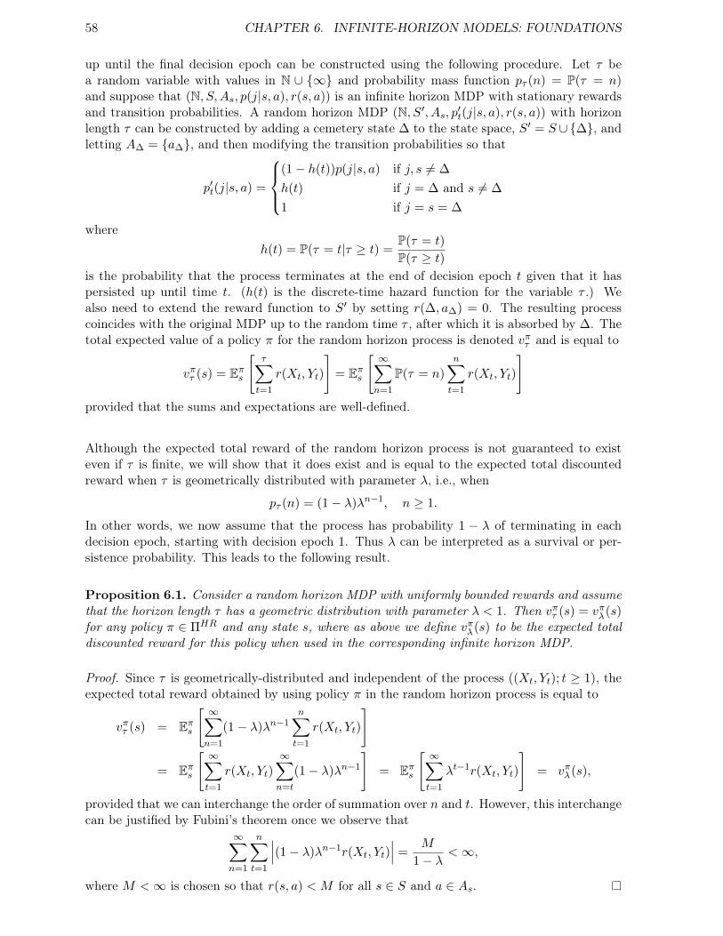
58 CHAPTER 6. INFINITE-HORIZON MODELS: FOUNDATIONS
up until the final decision epoch can be constructed using the following procedure. Let τ bea random variable with values in N ∪ {∞} and probability mass function pτ (n) = P(τ = n)and suppose that (N, S,As, p(j|s, a), r(s, a)) is an infinite horizon MDP with stationary rewardsand transition probabilities. A random horizon MDP (N, S′, As, p′t(j|s, a), r(s, a)) with horizonlength τ can be constructed by adding a cemetery state ∆ to the state space, S′ = S ∪{∆}, andletting A∆ = {a∆}, and then modifying the transition probabilities so that
p′t(j|s, a) =
(1− h(t))p(j|s, a) if j, s 6= ∆h(t) if j = ∆ and s 6= ∆1 if j = s = ∆
whereh(t) = P(τ = t|τ ≥ t) =
P(τ = t)P(τ ≥ t)
is the probability that the process terminates at the end of decision epoch t given that it haspersisted up until time t. (h(t) is the discrete-time hazard function for the variable τ .) Wealso need to extend the reward function to S′ by setting r(∆, a∆) = 0. The resulting processcoincides with the original MDP up to the random time τ , after which it is absorbed by ∆. Thetotal expected value of a policy π for the random horizon process is denoted vπτ and is equal to
vπτ (s) = Eπs
[τ∑t=1
r(Xt, Yt)
]= Eπs
[ ∞∑n=1
P(τ = n)n∑t=1
r(Xt, Yt)
]provided that the sums and expectations are well-defined.
Although the expected total reward of the random horizon process is not guaranteed to existeven if τ is finite, we will show that it does exist and is equal to the expected total discountedreward when τ is geometrically distributed with parameter λ, i.e., when
pτ (n) = (1− λ)λn−1, n ≥ 1.
In other words, we now assume that the process has probability 1 − λ of terminating in eachdecision epoch, starting with decision epoch 1. Thus λ can be interpreted as a survival or per-sistence probability. This leads to the following result.
Proposition 6.1. Consider a random horizon MDP with uniformly bounded rewards and assumethat the horizon length τ has a geometric distribution with parameter λ < 1. Then vπτ (s) = vπλ(s)for any policy π ∈ ΠHR and any state s, where as above we define vπλ(s) to be the expected totaldiscounted reward for this policy when used in the corresponding infinite horizon MDP.
Proof. Since τ is geometrically-distributed and independent of the process ((Xt, Yt); t ≥ 1), theexpected total reward obtained by using policy π in the random horizon process is equal to
vπτ (s) = Eπs
[ ∞∑n=1
(1− λ)λn−1n∑t=1
r(Xt, Yt)
]
= Eπs
[ ∞∑t=1
r(Xt, Yt)∞∑n=t
(1− λ)λn−1
]= Eπs
[ ∞∑t=1
λt−1r(Xt, Yt)
]= vπλ(s),
provided that we can interchange the order of summation over n and t. However, this interchangecan be justified by Fubini’s theorem once we observe that
∞∑n=1
n∑t=1
∣∣∣(1− λ)λn−1r(Xt, Yt)∣∣∣ =
M
1− λ<∞,
where M <∞ is chosen so that r(s, a) < M for all s ∈ S and a ∈ As.

6.4. OPTIMALITY CRITERIA 59
6.4 Optimality Criteria
An important difference between finite-horizon and infinite-horizon Markov decision problems isthat there are many more optimality criteria in use for the latter. Six of these are introduced inthe following definition and we will see even more below.
Definition 6.2. Suppose that π∗ ∈ ΠHR is a history-dependent, randomized policy for an infinite-horizon Markov decision process.
(1) The value of the MDP is defined to be the quantity
v∗(s) ≡ supπ∈ΠHR
vπ(s),
provided that the expected total reward vπ(s) exists for every policy π and every state s ∈ S.Furthermore, in this case, a policy π∗ is said to be total reward optimal if
vπ∗(s) ≥ vπ(s) for every s ∈ S and all π ∈ ΠHR.
(2) Let λ ∈ [0, 1) be given. The λ-discounted value of the MDP is defined to be the quantity
v∗λ(s) ≡ supπ∈ΠHR
vπλ(s),
provided that the expected total discounted reward vπλ(s) exists for every policy π and everystate s ∈ S. In this case, a policy π∗ is said to be discount optimal if
vπ∗
λ (s) ≥ vπλ(s) for every s ∈ S and all π ∈ ΠHR.
(3) The optimal gain of the MDP is defined to be the quantity
g∗(s) ≡ supπ∈ΠHR
vπ(s),
provided that the average gain gπ(s) exists for every policy π and every state s ∈ S. In thiscase, a policy π∗ is said to be gain optimal or average optimal if
gπ∗(s) ≥ gπ(s) for every s ∈ S and all π ∈ ΠHR.
(4) A policy π∗ is said to be limit point average optimal if
gπ∗− (s) = lim inf
N→∞
1Nvπ∗
N+1 ≥ lim supN→∞
1NvπN+1 = gπ+(s)
for every s ∈ S and all π ∈ ΠHR.
(5) A policy π∗ is said to be lim sup average optimal if
gπ∗
+ (s) ≥ gπ+(s) for every s ∈ S and all π ∈ ΠHR.
(6) Similarly, a policy π∗ is said to be lim inf average optimal if
gπ∗− (s) ≥ gπ−(s) for every s ∈ S and all π ∈ ΠHR.

60 CHAPTER 6. INFINITE-HORIZON MODELS: FOUNDATIONS
Notice that the optimality criteria defined in parts (1) - (3) can only be applied to Markovdecision problems that have the property that the limits used to define the expected total re-ward, the expected total discounted reward, or the average gain, respectively, exist for all policiesπ ∈ ΠHR. In contrast, the criteria defined in parts (4) - (6) can be applied to every MDP sincethese depend only on lim sup’s and lim inf’s, which always exist.
Example 6.2. Consider the infinite-horizon Markov decision process defined as follows:
• States: S = {s1, s2, s3};
• Action sets: As1 = {a1,1}, As2 = {a2,1, a2,2} and As3 = {a3,1};
• Transition probabilities: p(s2|s1, a11) = p(s1|s2, a2,1) = p(s3|s2, a2,2) = p(s2|s3, a3,1) = 1;
• Rewards: r(s1, a1,1) = r(s2, a2,2) = 0, r(s2, a2,1) = r(s3, a3,1) = 1.
The decision maker only has a choice to make in state s2 and this choice determines one of twostationary policies. Let d∞ be the stationary policy which uses action a2,1 and let e∞ be thestationary policy which uses action a2,2. Both of these policies have the same average gain
gd∞
(s) = ge∞
(s) = 0.5
and indeed it can be shown that gπ(s) = 0.5 for any policy π ∈ ΠHR since every policy earnsits user exactly 1 unit of reward every second decision epoch. This shows that every policy isaverage optimal for this MDP. On the other hand, different policies can generate different rewardstreams, e.g., if we start in state s2, then policy d∞ generates the reward stream (1, 0, 1, 0, · · · )while e∞ generates the reward stream (0, 1, 0, 1, · · · ).
Example 6.2 demonstrates that the average reward criterion is unselective because this criteriafails to differentiate between optimal policies that generate different reward streams. In suchcases, it may be necessary to turn to one of the alternative optimality criteria described below.
Definition 6.3. A policy π∗ is said to be overtaking optimal if
lim infN→∞
[vπ∗
N (s)− vπN (s)]≥ 0
for all π ∈ ΠHR and all s ∈ S.
Since this criterion is defined in terms of a lim inf, it is applicable to all MDPs. For example,in Example 6.2 the stationary policies d∞ and e∞ generate the following reward streams whenbeginning in state s2:
vd∞N (s2) : 1, 1, 2, 2, 3, 3, · · ·ve∞N (s2) : 0, 1, 1, 2, 2, 3, · · ·
vd∞N (s2)− ve∞N (s2) : 1, 0, 1, 0, · · · .
Thus
lim infN→∞
(vd∞N (s)− ve∞N (s)
)= 0
lim infN→∞
(ve∞N (s)− vd∞N (s)
)= −1

6.5. MARKOV POLICIES 61
and so d∞ is overtaking optimal.
There are several other variants of overtaking optimality, all of which are based on comparisonsof the limit points of the reward sequence or average reward sequence. An alternative approachis to base optimality on the limiting behavior of the discounted rewards as the discount rate λincreases to 1. These are called sensitive discount optimality criteria.
Definition 6.4. As above, let π∗ be a policy for an infinite-horizon MDP.
1. π∗ is said to be n-discount optimal for a constant n ≥ −1 if
lim infλ↑1
(1− λ)−n[vπ∗
λ (s)− vπλ(s)]≥ 0
for all π ∈ ΠHR and all s ∈ S. Furthermore, if π∗ is 0-discount optimal, then π∗ is alsosaid to be bias optimal.
2. π∗ is said to be ∞-discount optimal if it is n-discount optimal for all n ≥ −1.
3. π∗ is said to be 1-optimal or Blackwell optimal if for each s ∈ S there exists a λ∗(s)such that
vπ∗
λ (s)− vπλ(s) ≥ 0
for all π ∈ ΠHR and all λ ∈ [λ∗(s), 1). Furthermore, if the quantity λ∗ ≡ sups λ∗(s) < 1,then the policy is said to be strongly Blackwell optimal.
Notice that if n1 > n2 then n1-discount optimality implies n2-discount optimality, i.e., n1-discount optimality is more sensitive than n2-discount optimality. Furthermore, Blackwell opti-mality implies n-discount optimality for all n ≥ 1.
6.5 Markov policies
Our aim in this section is to show that for any stationary infinite-horizon Markov decision problemthere is always a randomized Markov policy which has the same expected total reward, the sameexpected total discounted reward, and also the same average award. Later, we will show that wecan also replace randomized policies by deterministic policies for most Markov decision problems.
Theorem 6.1. Let π = (d1, d2, · · · ) ∈ ΠHR. Then, for each s ∈ S, there exists a policyπ′ = (d1, d2, · · · ) ∈ ΠMR satisfying
Pπ′ {Xt = j, Yt = a|X1 = s} = Pπ {Xt = j, Yt = a|X1 = s} (6.7)
for every t ≥ 1.
Proof. Fix s ∈ S and define the randomized Markov decision rule d′t by
qd′t(j)(a) ≡ Pπ {Yt = a|Xt = j,X1 = s}
for j ∈ S and t ≥ 1. Let π′ = (d′1, d′2, · · · ) ∈ ΠMR and observe that
Pπ′ {Yt = a|Xt = j} = Pπ
′ {Yt = a|Xt = j,X1 = s}= Pπ {Yt = a|Xt = j,X1 = s} .

62 CHAPTER 6. INFINITE-HORIZON MODELS: FOUNDATIONS
We show that the identity (6.7) holds by (forward) induction on t. First, observe that whent = 1, this identity follows from the fact that
Pπ′ {X1 = j, Y1 = a|X1 = s} = Pπ
′ {Y1 = a|X1 = s}= Pπ {Y1 = a|X1 = s} = Pπ {X1 = j, Y1 = a|X1 = s} ,
which is clearly true. Next, suppose that (6.7) holds for t = 1, · · · , n− 1. Then
Pπ′ {Xn = j|X1 = s} =
∑k∈S
∑a∈Ak
Pπ′ {Xn−1 = k, Yn−1 = a|X1 = s} p(j|k, a)
=∑k∈S
∑a∈Ak
Pπ {Xn−1 = k, Yn−1 = a|X1 = s} p(j|k, a)
= Pπ {Xn = j|X1 = s} ,
where the second inequality follows from the induction hypothesis. Consequently,
Pπ′ {Xn = j, Yn = a|X1 = s} = Pπ
′ {Yn = a|Xn = j}Pπ′ {Xn = j|X1 = s}
= Pπ′ {Yn = a|Xn = j}Pπ
′ {Xn = j|X1 = s}= Pπ {Xn = j, Yn = a|X1 = s} ,
which completes the induction argument.
A similar result holds when the initial state of the MDP is itself randomly distributed.
Corollary 6.1. For each distribution ν of X1 and any history-dependent policy π, there existsa randomized Markov policy π′ for which
Pπ′ {Xt = j, Yt = a} = Pπ {Xt = j, Yt = a}
for all j ∈ S, a ∈ Aj, and t ≥ 1.
It should be emphasized that Theorem 6.1 and Corollary 6.1 only guarantee that the marginalprobabilities Pπ′ {Xt = j, Yt = a} (also known as the state-action frequencies) are the sameas those obtained under policy π. In contrast, the joint probabilities of the states and/or actionsat multiple decision epochs will usually differ between the two policies. However, the equivalenceof the marginal probabilities is enough to ensure that the expected value, expected discountedvalue, and the expected gain are the same under either policy since the expectations
vπN (s) =N−1∑t=1
∑j∈S
∑a∈Aj
r(j, a)P(Xt = j, Yt = a)
vπλ(s) =∞∑t=1
∑j∈S
∑a∈Aj
λt−1r(j, a)P(Xt = j, Yt = a),
only depend on the state-action frequencies.
Theorem 6.2. Given any π ∈ ΠHR and any s ∈ S, there exists a policy π′ ∈ ΠMR such that
(a) vπ′N (s) = vπN (s) for N ≥ 1 and vπ′(s) = vπ(s) when the relevant limits exist;
(b) vπ′λ (s) = vπλ(s) for λ ∈ [0, 1);
(c) gπ′± (s) = gπ±(s) and gπ′(s) = gπ(s), when the relevant limits exist.
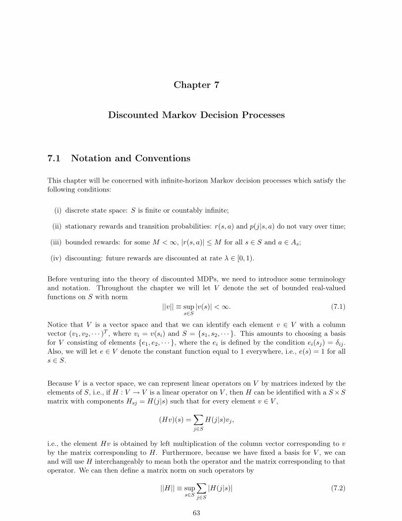
Chapter 7
Discounted Markov Decision Processes
7.1 Notation and Conventions
This chapter will be concerned with infinite-horizon Markov decision processes which satisfy thefollowing conditions:
(i) discrete state space: S is finite or countably infinite;
(ii) stationary rewards and transition probabilities: r(s, a) and p(j|s, a) do not vary over time;
(iii) bounded rewards: for some M <∞, |r(s, a)| ≤M for all s ∈ S and a ∈ As;
(iv) discounting: future rewards are discounted at rate λ ∈ [0, 1).
Before venturing into the theory of discounted MDPs, we need to introduce some terminologyand notation. Throughout the chapter we will let V denote the set of bounded real-valuedfunctions on S with norm
||v|| ≡ sups∈S|v(s)| <∞. (7.1)
Notice that V is a vector space and that we can identify each element v ∈ V with a columnvector (v1, v2, · · · )T , where vi = v(si) and S = {s1, s2, · · · }. This amounts to choosing a basisfor V consisting of elements {e1, e2, · · · }, where the ei is defined by the condition ei(sj) = δij .Also, we will let e ∈ V denote the constant function equal to 1 everywhere, i.e., e(s) = 1 for alls ∈ S.
Because V is a vector space, we can represent linear operators on V by matrices indexed by theelements of S, i.e., if H : V → V is a linear operator on V , then H can be identified with a S×Smatrix with components Hsj = H(j|s) such that for every element v ∈ V ,
(Hv)(s) =∑j∈S
H(j|s)vj ,
i.e., the element Hv is obtained by left multiplication of the column vector corresponding to vby the matrix corresponding to H. Furthermore, because we have fixed a basis for V , we canand will use H interchangeably to mean both the operator and the matrix corresponding to thatoperator. We can then define a matrix norm on such operators by
||H|| ≡ sups∈S
∑j∈S|H(j|s)| (7.2)
63

64 CHAPTER 7. DISCOUNTED MARKOV DECISION PROCESSES
and we will say that H is a bounded linear operator if ||H|| <∞. For example, if S is finite, thenall linear operators on V are bounded. Likewise, every stochastic matrix P on S corresponds toa bounded linear operator on V with norm ||P || = 1.
The matrix norm defined in (7.2) has several important properties. First note that it is consistentwith the norm on V is the sense that if H is a bounded linear operator on V , then for any elementv ∈ V , we have
||Hv|| = sups∈S|(Hv)(s)| = sup
s∈S
∣∣∣∣∣∣∑j∈S
H(j|s)vj
∣∣∣∣∣∣ ≤ sups
∑j∈S|H(j|s)| · ||v|| = ||H|| · ||v||.
Similarly, it can be shown that if A and B are bounded linear operators on V , then both thesum A+B and the product AB are bounded linear operators on V and
||A+B|| ≤ ||A||+ ||B|| (7.3)||AB|| ≤ ||A|| · ||B|| (7.4)
so that, in particular,||An|| ≤ ||A||n
for any positive integer n ≥ 1. Here, the product of two bounded linear operators A and B isdefined both in a functional sense, i.e., AB is the operator which maps an element v ∈ V to theelement A(Bv), and in an algebraic sense via matrix multiplication of the matrices representingthe two operators. Furthermore, we say that a sequence of bounded linear operators (Hn;n ≥ 1)converges in norm to a bounded linear operator H if the following is true
limn→∞
||Hn −H|| = 0;
notice, as well, that convergence in norm implies that
limn→∞
||Hnv −Hv|| = 0
for all v ∈ V . The set of all bounded linear operators on V is said to be a Banach algebra,meaning that it is a normed vector space which is complete (i.e., all Cauchy sequences converge)and which satisfies inequality (7.4).
Given a MDP satisfying the above assumptions and a Markovian decision rule d for that process,let the quantities rd(s) and pd(s) be defined by
rd(s) ≡ r(s, d(s)) and pd(j|s) ≡ p(j|s, d(s))
if d ∈ DMD is deterministic, or
rd(s) ≡∑a∈As
qd(s)(a)r(s, a) and pd(j|s) ≡∑a∈As
qd(s)(a)p(j|s, a)
if d ∈ DMR is randomized. In either case, let rd ∈ V be the vector with components rd(s) andlet Pd be the stochastic matrix with components pd(j|s). We will call rd the reward vectorand Pd the transition probability matrix corresponding to the decision rule d. For futurereference, notice that if v ∈ V , then rd + λPdv ∈ V .
If π = (d1, d2, · · · ) is a Markovian policy (randomized or deterministic), then the (s, j) componentof the t-step transition matrix P tπ is given by the following formula:
P tπ(j|s) ≡ Pπ(Xt+1 = j|X1 = s) = [Pd1Pd2 · · ·Pdt ] (j|s),

7.2. POLICY EVALUATION 65
where [Pd1Pd2 · · ·Pdt ] is the product of the first t transition matrices. In fact, the processes(Xt; t ≥ 1) and ((Xt, rdt(Xt)); t ≥ 1) are both Markov processes under the probability distribu-tion induced by π, and if v ∈ V is a bounded function defined on S then the expected value ofthe quantity v(Xt) can be calculated using the formula
Eπs [v(Xt)] = P t−1π v(s) =
∑j∈S
P t−1π (j|s)v(j)
Furthermore, the expected total discounted reward of policy π can be calculated using the formula
vπλ = Eπ[ ∞∑t=1
λt−1rt(Xt, Yt)
]=
∞∑t=1
λt−1P t−1π rdt .
7.2 Policy Evaluation
Suppose that π = (d1, d2, · · · ) ∈ ΠMR is a Markovian policy for a MDP and observe that theexpected total discounted reward for π can be expressed as
vπλ =∞∑t=1
λt−1P t−1π rdt
= rd1 + λPd1rd2 + λ2Pd1Pd2rd3 + λ3Pd1Pd2Pd3rd4 · · ·= rd1 + λPd1
(rd2 + λPd2rd3 + λ2Pd2Pd3rd4 · · ·
),
which we can rewrite asvπλ = rd1 + λPd1v
π′λ , (7.5)
where π′ = (d2, d3, · · · ) is the policy derived from π by dropping the first decision rule andexecuting each of the remaining rules one epoch earlier than prescribed by π. This identity canbe expressed component-wise as
vπλ(s) = rd1(s) + λ∑j∈S
pd1(j|s)vπ′λ (j),
and we refer to this system of equations as the policy evaluation equations.
If π = d∞ is a stationary policy, then π′ = π and so the reward vector v = vd∞λ satisfies the
equationv = rd + λPdv.
Equivalently, if we define the operator Ld : V → V by
Ldv ≡ rd + λPdv, (7.6)
then it follows that vd∞λ is a fixed point of Ld, i.e., vd∞
= Ldvd∞ . In fact, it can be shown that
Ld has a unique fixed point in V , which therefore must be vd∞λ . This is a consequence of thefact that because Pd is a stochastic matrix, the operator I − λPd is a contraction on V for anyλ ∈ (0, 1), i.e.,
||I − λPd|| < 1,
and therefore I−λPd is invertible. Here I is the identity operator on V , i.e., Iv = v for all v ∈ V .

66 CHAPTER 7. DISCOUNTED MARKOV DECISION PROCESSES
Theorem 7.1. For any stationary policy d∞ ∈ ΠMR and any λ ∈ [0, 1), the expected totaldiscounted value vd∞λ is the unique fixed point in V of the operator Ld defined in (7.6) and isequal to
vd∞λ = (I − λPd)−1rd =
∞∑t=1
λt−1P t−1d rd,
where the infinite series is guaranteed to converge in norm.
Example: We can illustrate this result with the two-state MDP described in Section 4.1 (pp.23 - 24 of these notes). For ease of reference, we recall the formulation of this problem:
• States: S = {s1, s2}.
• Actions: As1 = {a11, a12}, As2 = {a21}.
• Rewards:
r(s1, a11) = 5 r(s1, a12) = 10 r(s2, a21) = −1
• Transition probabilities:
pt(s1|s1, a11) = 0.5, pt(s2|s1, a11) = 0.5pt(s1|s1, a12) = 0, pt(s2|s1, a12) = 1pt(s1|s2, a21) = 0, pt(s2|s2, a21) = 1
There are exactly two Markovian deterministic policies: δ∞, which chooses action a11 in states1, and γ∞, which instead chooses action a12 in that state. The policy evaluation equations forδ∞ take the form
v(s1) = 5 + λ(0.5v(s1) + 0.5v(s2))v(s2) = −1 + λv(s2),
which shows thatvδ∞λ (s1) =
5− 5.5λ(1− 0.5λ)(1− λ)
, vδ∞λ (s2) = − 1
1− λ.
Similar calculations show that
vγ∞
λ (s1) =10− 11λ(1− λ)
, vγ∞
λ (s2) = − 11− λ
.
Comparing these, we see that vγ∞
λ (s1) ≥ vδ∞λ (s1) for all λ ∈ [0, 1).
The inverse operator (I − λPd)−1 will play an important role throughout this chapter and so wesummarize several of its properties in the following lemma. We will use the following notation: ifu, v ∈ V , then we write u ≥ v if u(s) ≥ v(s) for all s ∈ S. In particular, u ≥ 0 means that everyvalue u(s) is non-negative. We also write vT for the vector transpose of v, i.e., vT is a columnvector.
Lemma 7.1. For any d ∈ DMR,
(a) If u ≥ 0, then (I − λPd)−1u ≥ u.

7.3. OPTIMALITY EQUATIONS 67
(b) If u ≥ v, then (I − λPd)−1u ≥ (I − λPd)−1v.
(c) If u ≥ 0, then uT (I − λPd)−1 ≥ uT .
For a proof, see Appendix C of Puterman (2005). Because of (a), we say that (I − λPd)−1 is apositive operator and we write (I − λPd)−1 ≥ 0.
7.3 Optimality Equations
If we let vn(s) denote the finite-horizon discounted value of an optimal policy, we know from ourprevious work that vn(s) satisfies the optimality equations:
vn(s) = supa∈As
r(s, a) + λ∑j∈S
p(j|s, a)vn+1(j)
.
This suggests that the infinite-horizon discounted rewards v(s) = limn→∞ vn(s) will satisfy theequations
v(s) = supa∈As
r(s, a) + λ∑j∈S
p(j|s, a)v(j)
(7.7)
for every s ∈ S and we call these equations the optimality equations or Bellman equationsfor the infinite-horizon process.
It will be convenient to define a non-linear operator L on V by setting
Lv ≡ supd∈DMD
{rd + λPdv} , (7.8)
where the supremum is evaluated component-wise, i.e., for each s ∈ S. When the sup is attainedfor all v ∈ V we will also define the operator L on V by
Lv ≡ maxd∈DMD
{rd + λPdv} . (7.9)
The next result explains why it is enough to consider only Markovian deterministic decisionrules: in effect, we can always find a deterministic Markovian decision rule that performs as wellas any randomized Markovian decision rule.
Proposition 7.1. For all v ∈ V and 0 ≤ λ ≤ 1,
supd∈DMD
{rd + λPdv} = supd∈DMR
{rd + λPdv} .
Proof. Since DMD ⊂ DMR, the RHS is at least as large as the LHS. Let v ∈ V , δ ∈ DMR andobserve that
supa∈As
r(s, a) + λ∑j∈S
p(j|s, a)v(j)
≥ ∑a∈As
qδ(a)
r(s, a) + λ∑j∈S
p(j|s, a)v(j)
.
Since this holds for every s ∈ S, it follows that for any δ ∈ DMR,
supd∈DMD
{rd + λPdv} ≥ rδ + λPδv,
and thus the LHS is at least as large as the RHS.
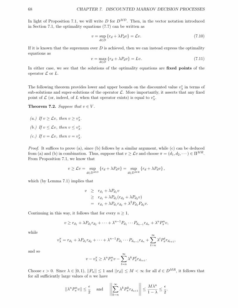
68 CHAPTER 7. DISCOUNTED MARKOV DECISION PROCESSES
In light of Proposition 7.1, we will write D for DMD. Then, in the vector notation introducedin Section 7.1, the optimality equations (7.7) can be written as
v = supd∈D{rd + λPdv} = Lv. (7.10)
If it is known that the supremum over D is achieved, then we can instead express the optimalityequations as
v = maxd∈D{rd + λPdv} = Lv. (7.11)
In either case, we see that the solutions of the optimality equations are fixed points of theoperator L or L.
The following theorem provides lower and upper bounds on the discounted value v∗λ in terms ofsub-solutions and super-solutions of the operator L. More importantly, it asserts that any fixedpoint of L (or, indeed, of L when that operator exists) is equal to v∗λ.
Theorem 7.2. Suppose that v ∈ V .
(a.) If v ≥ Lv, then v ≥ v∗λ.
(b.) If v ≤ Lv, then v ≤ v∗λ.
(c.) If v = Lv, then v = v∗λ.
Proof. It suffices to prove (a), since (b) follows by a similar argument, while (c) can be deducedfrom (a) and (b) in combination. Thus, suppose that v ≥ Lv and choose π = (d1, d2, · · · ) ∈ ΠMR.From Proposition 7.1, we know that
v ≥ Lv = supd∈DMD
{rd + λPdv} = supd∈DMR
{rd + λPdv} ,
which (by Lemma 7.1) implies that
v ≥ rd1 + λPd1v
≥ rd1 + λPd1(rd2 + λPd2v)= rd1 + λPd1rd2 + λ2Pd1Pd2v.
Continuing in this way, it follows that for every n ≥ 1,
v ≥ rd1 + λPd1rd2 + · · ·+ λn−1Pd1 · · ·Pdn−1rdn + λnPnπ v,
while
vπλ = rd1 + λPd1rd2 + · · ·+ λn−1Pd1 · · ·Pdn−1rdn +∞∑t=n
λtP tπrdt+1 ,
and so
v − vπλ ≥ λnPnπ v −∞∑t=n
λkP tπrdt+1 .
Choose ε > 0. Since λ ∈ [0, 1), ||Pn|| ≤ 1 and ||rd|| ≤ M < ∞ for all d ∈ DMR, it follows thatfor all sufficiently large values of n we have
||λnPnπ v|| ≤ε
2and
∣∣∣∣∣∣∣∣∣∣∞∑k=n
λkP kπ rdn+1
∣∣∣∣∣∣∣∣∣∣ ≤ Mλn
1− λ≤ ε
2.

7.3. OPTIMALITY EQUATIONS 69
Taken together, these two inequalities imply that
v(s) ≥ vπλ(s)− ε
for every s ∈ S and all ε > 0, and since π ∈ ΠMR is arbitrary, we then have
v(s) ≥ supπ∈ΠMR
vπλ(s) = v∗λ(s)
for every s ∈ S. This establishes (a).
To establish the existence of a solution to the optimality equations, we will appeal to a powerfulresult in fixed-point theory known as the Banach fixed-point theorem. Suppose that U is anormed vector space. A sequence (xn : n ≥ 1) ⊂ U is said to be a Cauchy sequence if forevery ε > 0 there is a positive integer N = N(ε) such that for all n,m ≥ N
||xn − xm|| < ε,
i.e., the sequence is Cauchy if for any ε > 0 there is a ball of radius ε such that all but finitelymany of the points in the sequence are contained in that ball. It can be shown, for instance,that any convergent sequence is a Cauchy sequence. If the converse is also true, i.e., if ev-ery Cauchy sequence in a normed vector space U converges to a point in U , then U is saidto be a Banach space. This is relevant to discounted Markov decision problems because thespace V of bounded real-valued functions, equipped with the supremum norm, is a Banach space.
We say that an operator T : V → V is a contraction mapping if there is a constant λ ∈ [0, 1)such that
||Tv − Tu|| ≤ λ||v − u||
for all u, v ∈ U . In other words, the distance between the points Tu and Tv is shrunk by at leasta factor λ relative to the distance between the points u and v. Notice that we do not require Tto be a linear mapping.
Theorem 7.3. (Banach Fixed-Point Theorem) Suppose that U is a Banach space and thatT : U → U is a contraction mapping. Then
(a.) T has a unique fixed point v∗ ∈ U : Tv∗ = v∗;
(b.) for any v0 ∈ U , the sequence (vn : n ≥ 0) defined by vn = T (vn−1) = Tn+1v0 converges innorm to v∗.
Proof. Let vn = Tn+1v0. Then, for any n,m ≥ 1,
||vn+m − vn|| ≤m−1∑k=0
||vn+k+1 − vn+k||
=m−1∑k=0
||Tn+kv1 − Tn+kv0||
≤m−1∑k=0
λn+k||v1 − v0||
= λn1− λm
1− λ||v1 − v0||,
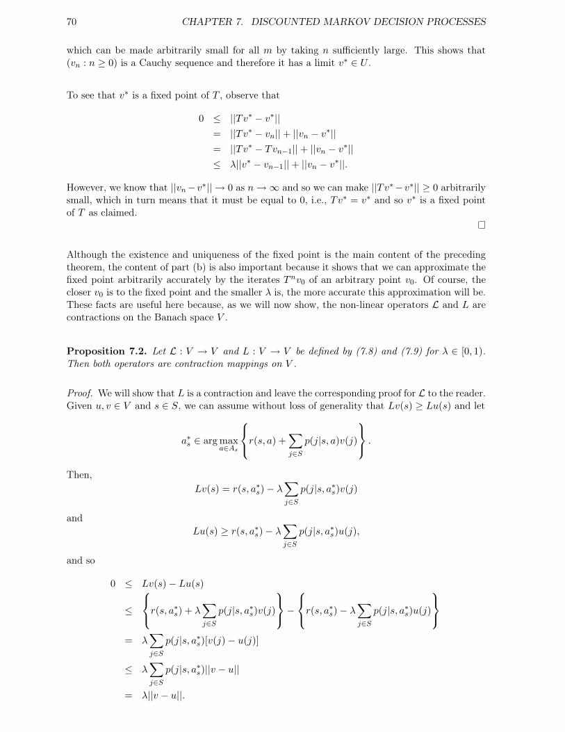
70 CHAPTER 7. DISCOUNTED MARKOV DECISION PROCESSES
which can be made arbitrarily small for all m by taking n sufficiently large. This shows that(vn : n ≥ 0) is a Cauchy sequence and therefore it has a limit v∗ ∈ U .
To see that v∗ is a fixed point of T , observe that
0 ≤ ||Tv∗ − v∗||= ||Tv∗ − vn||+ ||vn − v∗||= ||Tv∗ − Tvn−1||+ ||vn − v∗||≤ λ||v∗ − vn−1||+ ||vn − v∗||.
However, we know that ||vn−v∗|| → 0 as n→∞ and so we can make ||Tv∗−v∗|| ≥ 0 arbitrarilysmall, which in turn means that it must be equal to 0, i.e., Tv∗ = v∗ and so v∗ is a fixed pointof T as claimed.
Although the existence and uniqueness of the fixed point is the main content of the precedingtheorem, the content of part (b) is also important because it shows that we can approximate thefixed point arbitrarily accurately by the iterates Tnv0 of an arbitrary point v0. Of course, thecloser v0 is to the fixed point and the smaller λ is, the more accurate this approximation will be.These facts are useful here because, as we will now show, the non-linear operators L and L arecontractions on the Banach space V .
Proposition 7.2. Let L : V → V and L : V → V be defined by (7.8) and (7.9) for λ ∈ [0, 1).Then both operators are contraction mappings on V .
Proof. We will show that L is a contraction and leave the corresponding proof for L to the reader.Given u, v ∈ V and s ∈ S, we can assume without loss of generality that Lv(s) ≥ Lu(s) and let
a∗s ∈ arg maxa∈As
r(s, a) +∑j∈S
p(j|s, a)v(j)
.
Then,Lv(s) = r(s, a∗s)− λ
∑j∈S
p(j|s, a∗s)v(j)
andLu(s) ≥ r(s, a∗s)− λ
∑j∈S
p(j|s, a∗s)u(j),
and so
0 ≤ Lv(s)− Lu(s)
≤
r(s, a∗s) + λ∑j∈S
p(j|s, a∗s)v(j)
−r(s, a∗s)− λ∑
j∈Sp(j|s, a∗s)u(j)
= λ
∑j∈S
p(j|s, a∗s)[v(j)− u(j)]
≤ λ∑j∈S
p(j|s, a∗s)||v − u||
= λ||v − u||.

7.3. OPTIMALITY EQUATIONS 71
This shows that|Lv(s)− Lu(s)| ≤ λ||v − u||
for all s and taking the supremum over s ∈ S then gives
||Lv − Lu|| ≤ λ||v − u||.
Theorem 7.4. Suppose that S is countable, that the rewards are uniformly bounded, and thatλ ∈ [0, 1). Then
(a) There exists a unique element v∗ ∈ V satisfying Lv∗ = v∗ (or Lv∗ = v∗) and v∗ = v∗λ isthe discounted value of the Markov decision problem.
(b) For each d ∈ DMR, there exists a unique v ∈ V satisfying Ldv = v and v = vd∞λ is the
expected total discounted value of the stationary policy corresponding to d.
Proof. Since V is a Banach space and L and L are both contraction mappings on V , the Banachfixed-point theorem implies that each operator has a unique fixed point v∗. It then follows fromTheorem 7.2 that v∗ = v∗λ. Part (b) follows from (a) by taking D = {d} in the definitions of(7.10) and (7.11).
Although Theorem 7.4 tells us how (at least in principle) we may calculate the discounted valueof a Markov decision problem, it does not tell us whether discount-optimal policies exist or indeedhow to find them if they do exist. This issue is addressed by the next four theorems.
Theorem 7.5. A policy π∗ ∈ ΠHR is discount optimal if and only if vπ∗λ is a solution of theoptimality equation.
Proof. If π∗ is discount optimal, then vπ∗λ = v∗λ and so Theorem 7.4 (a) tells us that vπ∗λ is theunique fixed point of L, i.e., vπ∗λ is a solution of the optimality equation. Conversely, if vπ∗λ is afixed point of L, then Theorem 7.2 (c) tells us that vπ∗λ = v∗λ, which shows that π∗ is discount-optimal.
This shows that we can assess whether a policy is discount optimal by checking whether thediscounted value of that policy is a solution of the optimality equation.
Definition 7.1. Given v ∈ V , a decision rule dv ∈ DMD is said to be v-improving if
rdv + λPdvv = maxd∈DMD
{rd + λPdv} .
In particular, a decision rule d∗ ∈ DMD is said to be conserving for a λ-discounted Markovdecision problem if d∗ is v∗λ-improving.
The condition for dv to be v-improving can also be written as
Ldvv = Lv

72 CHAPTER 7. DISCOUNTED MARKOV DECISION PROCESSES
or, component-wise, as
r(s, dv(s)) + λ∑j∈S
p(j|s, dv(s))v(j) = maxa∈As
r(s, a) + λ∑j∈S
p(j|s, a)v(j)
.
Similarly, d∗ is conserving if and only if
Ld∗v∗ = rd∗ + λPd∗v
∗ = v∗.
Conserving rules are particularly important because they give rise to optimal policies that arealso stationary.
Theorem 7.6. Suppose that the supremum is attained in the optimality equations for everyv ∈ V . Then
(a) there exists a conserving decision rule d∗ ∈ DMD;
(b) if d∗ is conserving, the deterministic stationary policy (d∗)∞ is discount optimal;
(c) v∗λ = supd∈D vd∗λ .
Proof. Because we are assuming that the supremum is attained, we can define a decision rule d∗
by choosingd∗(s) ∈ arg max
a∈As{r(s, a) + λP (j|s, a)v∗λ(j)}
for each s ∈ S. It then follows that Ld∗v∗λ = v∗λ, which implies that d∗ is conserving and alsothat
vd∗λ = v∗λ.
This verifies both (a) and (b), while (c) follows from (b).
Theorem 7.7. Suppose that there exists either a conserving decision rule or an optimal policy.Then there exists a deterministic stationary policy which is optimal.
Proof. The sufficiency of the first claim follows from Theorem 7.6. Thus, suppose that π∗ =(d′, π′) is an optimal policy with d1 = d′ ∈ DMR. Then, since vπ′λ ≤ vπ∗λ and Pd′ is a positiveoperator,
v∗λ = rd′ + λPd′vπ′λ
≤ rd′ + λPd′vπ∗λ
≤ supd∈D
{rd + λPdv
π∗λ
}= v∗λ.
This implies thatrd′ + λPd′v
π∗λ = sup
d∈D
{rd + λPdv
π∗λ
},
which shows that d′ is a conserving decision rule and therefore (d′)(∞) is a stationary optimalpolicy by Theorem 7.6.
Theorem 7.8. Assume that S is discrete and that one of the following conditions holds:

7.4. VALUE ITERATION 73
(a) As is finite for every s ∈ S;
(b) As is compact for every s ∈ S, r(s, a) is continuous in a and for all j, s ∈ S p(j|s, a) iscontinuous in a.
Then there exists an optimal deterministic stationary policy.
The proof is similar to that given for Proposition 5.1.
The following example demonstrates that some Markov decision processes have no discountoptimal policies. Let S = {s}, As = {1, 2, 3, · · · } and r(s, a) = 1− 1/a. Then
v∗λ(s) = (1− λ)−1,
but no policy π exists with this value.
When optimal policies do not exist, we instead seek ε-optimal policies. A policy π∗ε is said tobe ε-optimal if for all s ∈ S
vπελ (s) ≥ v∗λ(s)− ε,
or equivalently,vπ∗ελ ≥ v
πλ − εe,
where e = (1, 1, · · · ) is a vector of 1’s.
Theorem 7.9. If S is countable, then for every ε > 0 there exists an ε-optimal decision rule.
Proof. Given ε > 0, choose a decision rule dε ∈ DMD such that
rdε + λPdεv∗λ ≥ v∗λ − (1− λ)εe.
Since
vd(∞)ελ = (I − λPdε)−1rdε
(I − λPdε)−1e = (1− λ)−1e,
it follows thatrdε ≥ (I − λPdε)−1v∗λ − (1− λ)εe,
andvd
(∞)ελ ≥ v∗λ − εe,
which shows that d(∞)ε is ε-optimal.
7.4 Value Iteration
The value iteration algorithm is a method that can be used to find ε-optimal policies fordiscounted Markov decision processes. The algorithm consists of the following steps:
(1) Set n = 0 and choose an error tolerance ε > 0 and an initial condition v0 ∈ V .

74 CHAPTER 7. DISCOUNTED MARKOV DECISION PROCESSES
(2) For each s ∈ S, compute vn+1(s) by
vn+1(s) = maxa∈As
r(s, a) + λ∑j∈S
p(j|s, a)v(n)(j)
(3) If
||vn+1 − vn|| < ε(1− λ)2λ
,
go to step 4. Otherwise increase n to n+ 1 and return to step 2.
(4) For each s ∈ S, choose
dε(s) ∈ arg maxa∈As
r(s, a) + λ∑j∈S
p(j|s, a)vn+1(j)
and stop.
In vector notation, this algorithm can be expressed as:
vn+1 = Lvn
dε ∈ arg maxd∈D
{rd + λPdv
n+1}.
The fact that value iteration leads to an ε-optimal policy is established in the proof of the nexttheorem.
Theorem 7.10. Given v0 and ε > 0, let (vn : n ≥ 0) be the sequence of values and dε thedecision rule produced by the value iteration algorithm. Then
(a) vn converges in norm to v∗λ;
(b) the stationary policy d(∞)ε is ε-optimal;
(c) ||vn+1 − v∗λ|| < ε/2 for any n that satisfies the inequality in step 3.
Proof. Convergence of the values vn to the fixed point v∗λ follows from the Banach fixed-pointtheorem. Choose n so that the condition
||vn+1 − vn|| < ε(1− λ)2λ
,
is satisfied. Then||vd
(∞)ελ − v∗λ|| ≤ ||v
d(∞)ελ − vn+1||+ ||vn+1 − v∗λ||.
Since vd(∞)ελ is a fixed point of Ldε and Ldεvn+1 = Lvn+1, it follows that
||vd(∞)ελ − vn+1|| = ||Ldεv
d(∞)ελ − vn+1||
≤ ||Ldεvd(∞)ελ − Ldεvn+1||+ ||Ldεvn+1 − vn+1||
= ||Ldεvd(∞)ελ − Ldεvn+1||+ ||Lvn+1 − Lvn||
≤ λ||vd(∞)ελ − vn+1||+ λ||vn+1 − vn||.
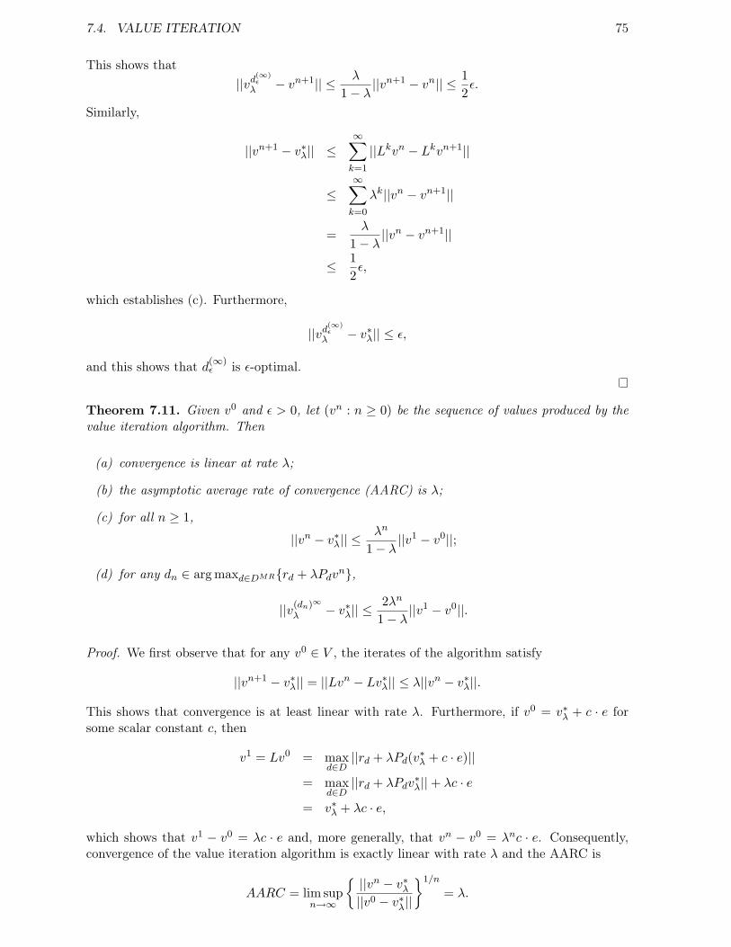
7.4. VALUE ITERATION 75
This shows that||vd
(∞)ελ − vn+1|| ≤ λ
1− λ||vn+1 − vn|| ≤ 1
2ε.
Similarly,
||vn+1 − v∗λ|| ≤∞∑k=1
||Lkvn − Lkvn+1||
≤∞∑k=0
λk||vn − vn+1||
=λ
1− λ||vn − vn+1||
≤ 12ε,
which establishes (c). Furthermore,
||vd(∞)ελ − v∗λ|| ≤ ε,
and this shows that d(∞)ε is ε-optimal.
Theorem 7.11. Given v0 and ε > 0, let (vn : n ≥ 0) be the sequence of values produced by thevalue iteration algorithm. Then
(a) convergence is linear at rate λ;
(b) the asymptotic average rate of convergence (AARC) is λ;
(c) for all n ≥ 1,
||vn − v∗λ|| ≤λn
1− λ||v1 − v0||;
(d) for any dn ∈ arg maxd∈DMR{rd + λPdvn},
||v(dn)∞
λ − v∗λ|| ≤2λn
1− λ||v1 − v0||.
Proof. We first observe that for any v0 ∈ V , the iterates of the algorithm satisfy
||vn+1 − v∗λ|| = ||Lvn − Lv∗λ|| ≤ λ||vn − v∗λ||.
This shows that convergence is at least linear with rate λ. Furthermore, if v0 = v∗λ + c · e forsome scalar constant c, then
v1 = Lv0 = maxd∈D||rd + λPd(v∗λ + c · e)||
= maxd∈D||rd + λPdv
∗λ||+ λc · e
= v∗λ + λc · e,
which shows that v1 − v0 = λc · e and, more generally, that vn − v0 = λnc · e. Consequently,convergence of the value iteration algorithm is exactly linear with rate λ and the AARC is
AARC = lim supn→∞
{||vn − v∗λ||v0 − v∗λ||
}1/n
= λ.

76 CHAPTER 7. DISCOUNTED MARKOV DECISION PROCESSES
To verify (c), observe that
||vn − v∗λ|| ≤ ||vn − vn+1||+ ||vn+1 − v∗λ||= ||Lnv0 − Lnv1||+ ||Lvn − Lv∗λ||≤ λn||v1 − v0||+ λ||vn − v∗λ||.
This can be rearranged to give
||vn − v∗λ|| ≤λn
1− λ||v1 − v0||.
The number of iterations required to arrive at an ε-optimal policy can be estimated with thehelp of part (d) of Theorem 7.11 by setting
ε =2λn
1− λ||v1 − v0||
and then solving for n. This gives the formula
n ≈ln(
ε(1−λ)2||v1−v0||
)ln(λ)
which, as expected, diverges as λ approaches 1. For example, if ε = 0.01, λ = 0.95 and||v1−v0|| = 1, then approximately n = 162 iterations will be required to find an ε-optimal policy.
Splitting Methods: The efficiency of the value iteration algorithm can sometimes be improvedby using a technique from numerical linear algebra known as splitting. Suppose that the statespace S = {s1, · · · , sN is finite. To illustrate this approach, we will describe the Gauss-Seidelvalue iteration algorithm, which consists of the following steps:
(1) Set n = 0 and choose an error tolerance ε > 0 and an initial condition v0 ∈ V .
(2) For each value of j = 1, · · · , N , compute vn+1(sj) by
vn+1(sj) = maxa∈Asj
r(sj , a) + λ
∑i<j
p(i|s, a)v(n+1)(i) + λ∑i≥j
p(i|s, a)v(n)(i)
.
(3) If
||vn+1 − vn|| < ε(1− λ)2λ
,
go to step 4. Otherwise increase n to n+ 1 and return to step 2.
(4) For each s ∈ S, choose
dε(s) ∈ arg maxa∈As
r(s, a) + λ∑j∈S
p(j|s, a)vn+1(j)
and stop.

7.5. POLICY ITERATION 77
The only difference between the ordinary value iteration algorithm and the variant based on theGauss-Seidel method comes in step 2 where the latter algorithm replaces the current estimatevn(si) of the value of state si by the new estimate vn+1(si) as soon as it becomes available. Itcan be shown that this algorithm converges to the optimal value v∗λ, that its order of convergenceis linear, and that the rate of convergence is less than or equal to λ. Furthermore, for manyproblems, the rate of convergence is strictly less than λ, which means that the Gauss-Seidelalgorithm is then strictly better than the ordinary value iteration.
7.5 Policy Iteration
Policy iteration works by constructing a sequence of policies with monotonically increasing re-wards. Throughout this section we will assume that every vector v ∈ V has an improving decisionrule dv ∈ DMD, i.e.
dv ∈ arg maxd∈DMD
{rd + λPdv}
or equivalently
dv(s) ∈ arg maxa∈As
r(s, a) + λ∑j∈S
p(j|s, a)v(j)
for every s ∈ S. This will hold, for instance, if the action sets As are finite. The policy iterationalgorithm consists of the following steps:
(1) Set n = 0 and choose an initial decision rule d0 ∈ DMD.
(2) Policy evaluation: Obtain vn = vd(∞)nλ by solving the linear equation
(I − λPdn)vn = rdn .
(3) Policy improvement: Choose dn+1 so that
dn+1 ∈ arg maxd∈DMD
{rd + λPdvn} ,
setting dn+1 = dn whenever possible.
(4) If dn+1 = dn, stop and set d∗ = dn. Otherwise, increase n by 1 and return to step 2.
An important property of the policy iteration algorithm is that the sequence of values vn gener-ated by the algorithm is non-decreasing. This is a consequence of the policy improvement step,which always selects a rule that is at least as good as the current rule.
Proposition 7.3. Let vn and vn+1 be successive values generated by the policy iteration algo-rithm. Then vn+1 ≥ vn.
Proof. If dn+1 is a decision rule generated by the policy evaluation algorithm, then the policyimprovement step and the fact that Ldnvn = vn imply that
rdn+1 + λPdn+1vn ≥ rdn + λPdnv
n = vn.
This shows thatrdn+1 ≥ (I − λPdn+1)vn
and consequentlyvn+1 = (I − λPdn+1)−1rdn+1 ≥ vn.
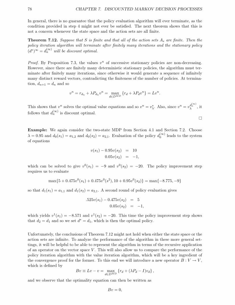
78 CHAPTER 7. DISCOUNTED MARKOV DECISION PROCESSES
In general, there is no guarantee that the policy evaluation algorithm will ever terminate, as thecondition provided in step 4 might not ever be satisfied. The next theorem shows that this isnot a concern whenever the state space and the action sets are all finite.
Theorem 7.12. Suppose that S is finite and that all of the action sets As are finite. Then thepolicy iteration algorithm will terminate after finitely many iterations and the stationary policy(d∗)∞ = d
(∞)n will be discount optimal.
Proof. By Proposition 7.3, the values vn of successive stationary policies are non-decreasing.However, since there are finitely many deterministic stationary policies, the algorithm must ter-minate after finitely many iterations, since otherwise it would generate a sequence of infinitelymany distinct reward vectors, contradicting the finiteness of the number of policies. At termina-tion, dn+1 = dn and so
vn = rdn + λPdnvn = max
d∈DMD{rd + λPdv
n} = Lvn.
This shows that vn solves the optimal value equations and so vn = v∗λ. Also, since vn = vd
(∞)nλ , it
follows that d(∞)n is discount optimal.
Example: We again consider the two-state MDP from Section 4.1 and Section 7.2. Chooseλ = 0.95 and d0(s1) = a1,2 and d0(s2) = a2,1. Evaluation of the policy d(∞)
0 leads to the systemof equations
v(s1)− 0.95v(s2) = 100.05v(s2) = −1,
which can be solved to give v0(s1) = −9 and v0(s2) = −20. The policy improvement steprequires us to evaluate
max{5 + 0.475v0(s1) + 0.475v0(s2), 10 + 0.95v0(s2)} = max{−8.775,−9}
so that d1(s1) = a1,1 and d1(s2) = a2,1. A second round of policy evaluation gives
.525v(s1)− 0.475v(s2) = 50.05v(s2) = −1,
which yields v1(s1) = −8.571 and v1(s2) = −20. This time the policy improvement step showsthat d2 = d1 and so we set d∗ = d1, which is then the optimal policy.
Unfortunately, the conclusions of Theorem 7.12 might not hold when either the state space or theaction sets are infinite. To analyze the performance of the algorithm in these more general set-tings, it will be helpful to be able to represent the algorithm in terms of the recursive applicationof an operator on the vector space V . This will also allow us to compare the performance of thepolicy iteration algorithm with the value iteration algorithm, which will be a key ingredient ofthe convergence proof for the former. To this end we will introduce a new operator B : V → V ,which is defined by
Bv ≡ Lv − v = maxd∈DMD
{rd + (λPd − I)vd} ,
and we observe that the optimality equation can then be written as
Bv = 0,

7.5. POLICY ITERATION 79
i.e., the value of the discounted Markov decision problem is the unique root of the operator B.Below, we will show that the policy evaluation algorithm can be interpreted as a generalizedform of Newton’s method applied to this root-finding problem. We begin with a proposition thatshows that B satisfies a generalized notion of convexity. To this end, given v ∈ V , let Dv be thecollection of v-improving decision rules, i.e., dv ∈ Dv if and only if
dv ∈ arg maxd∈DMD
{rd + λPdv} = arg maxd∈DMD
{rd + λ(Pd − I)v} .
We will refer to Dv as the set of supporting decision rules at v and we will say that λPdv − Iis the support of B at v.
Proposition 7.4. (Support inequality) For u, v ∈ V and dv ∈ Dv, we have
Bu ≥ Bv + (λPdv − I)(u− v).
Proof. The result in a consequence of the following identities/inequalities:
Bu ≥ rdv + (λPdv − I)uBv = rdv + (λPdv − I)v.
The next theorem shows how the operator B can be used to give a recursive representation ofthe policy iteration algorithm. As explained below, this representation can also be interpretedas an application of Newton’s method to B.
Theorem 7.13. Suppose that the sequence (vn;n ≥ 0) is generated by the policy iteration algo-rithm. Then, for any supporting rule dvn ∈ Dvn, we have
vn+1 = vn − (λPdvn − I)−1Bvn
Proof. By the definition of Dvn , we have
vn+1 = (I − λPdvn )−1 rdvn − vn + vn
= (I − λPdvn )−1 [rdvn + (λPdvn − I) vn]
+ vn
= vn − (I − λPdvn )−1Bvn.
To understand the connection with Newton’s method, recall that if f is a continuously differ-entiable function on R, then Newton’s method generates the sequence (xn;n ≥ 0) using therecursion
xn+1 = xn −f(xn)f ′(xn)
;
geometrically, this amounts to following the line tangent to the graph of f at xn down to itsintersection with the x-axis, which is then xn+1. In Theorem 7.13, the support λPdvn − I playsthe role of the derivative (or Jacobean) of the function B.
Our next results are concerned with the convergence of the policy iteration algorithm. DefineVB ≡ {v ∈ V : Bv ≥ 0}. It follows from Theorem 7.2 that if v ∈ VB, then Lv ≥ v and so v ≤ v∗λ,i.e., v is a lower bound for v∗λ.

80 CHAPTER 7. DISCOUNTED MARKOV DECISION PROCESSES
Lemma 7.2. Let v ∈ VB and dv ∈ Dv. Then
(a) Zv ≡ v + (I − λPdv)−1Bv ≥ Lv;
(b) Zv ∈ VB;
(c) Zv ≥ v.
Proof. Since Bv ≥ 0, Lemma 7.1 tells us that (I − λPdv)−1Bv ≥ 0 and so
Zv = v + (I − λPdv)−1Bv ≥ v +Bv = Lv.
Furthermore, by the support inequality for B (Proposition 7.4), we have
B(Zv) ≥ Bv + (λPdv − I)(Zv − v) = Bv −Bv = 0.
Part (c) follows from the assumption that Bv ≥ 0.
Theorem 7.14. The sequence of values (vn;n ≥ 0) generated by the policy iteration algorithmconverges monotonically and in norm to v∗λ.
Proof. Let un = Lnv0 be the sequence of values generated by the value iteration algorithm. Wewill use induction to show that un ≤ vn ≤ v∗λ and vn ∈ VB for all n ≥ 0. First observe that
Bv0 = maxd∈DMD
{rd + (λPd − I)v0
}≥ rd0 + (λPd0 − I)v0 = 0,
so that v0 ∈ VB and consequently v0 ≤ v∗λ. Since u0 = v0, this verifies the induction hypothesis
when n = 0.
Now assume that the hypothesis holds for all 0 ≤ k ≤ n for some n. Since vn+1 = Zvn, Lemma7.2 implies that vn+1 ∈ VB, vn ≤ v∗λ, and vn+1 ≥ Lvn ≥ Lun = un+1. This completes theinduction.
The theorem conclusion then follows from the fact that the sequence (un;n ≥ 0) converges to v∗λin norm.
Since value iteration has linear convergence, it follows that policy iteration has at least this orderof convergence. In fact, our next result shows that the order of convergence can be quadraticunder some conditions.
Theorem 7.15. Suppose that the sequence (vn;n ≥ 0) is generated by the policy iteration algo-rithm, that dvn ∈ Dvn is a supporting decision rule for each n ≥ 0, and that there exists a finitepositive number K ∈ (0,∞) such that
||Pdvn − Pdv∗λ|| ≤ K||vn − v∗λ||.
Then
||vn+1 − v∗λ|| ≤Kλ
1− λ||vn − v∗λ||2.

7.6. MODIFIED POLICY ITERATION 81
Proof. If we define the operators
Un ≡ (λPdvn − I) and U∗ ≡ (λPdv∗λ− I),
then the support inequality implies that
Bvn ≥ Bv∗λ + U∗(vn − v∗λ) = U∗(vn − v∗λ)
which along with the positivity of −U−1n gives
U−1n Bvn ≤ U−1
n U∗(vn − v∗λ).
Since the values vn generated by the policy iteration algorithm increase monotonically to v∗λ, itfollows that
0 ≤ v∗λ − vn+1
= v∗λ − vn + U−1n Bvn
≤ U−1n Un(v∗λ − vn)− U−1
n U∗(v∗λ − vn).
This implies that||v∗λ − vn+1|| ≤ ||U−1
n || ||Un − U∗|| ||v∗λ − vn||.However, since
||U−1n || ≤
11− λ
and||Un − U∗λ || = λ||Pdvn − Pdv∗
λ||,
the result then follows from the assumption that ||Pdvn − Pdv∗λ|| ≤ K||vn − v∗λ||.
Corollary 7.1. Suppose that there exists a positive constant K ∈ (0,∞) such that
||Pdv − Pdu || ≤ K||v − u||
holds for all u, v ∈ V whenever du ∈ Du and dv ∈ Dv. Then the conditions of Theorem 7.15 aresatisfied and so the policy iteration algorithm converges quadratically.
Sufficient conditions for this inequality to hold are that for each s ∈ S,
(i) As is compact and convex,
(ii) p(j|s, a) is affine in a, and
(iii) r(s, a) is strictly concave and twice continuously differentiable in a.
7.6 Modified Policy Iteration
Although the policy iteration algorithm has quadratic convergence, the actual numerical imple-mentation of this algorithm may be computationally expensive due to the need to solve a linearequation,
(I − λPdn)v = rdn ,
during the evaluation step of each iteration. Fortunately, in many problems, it suffices to findan approximate solution to this equation, which can be done much more efficiently. This is themotivation for the modified policy iteration algorithm, which combines features of boththe value iteration algorithm and the policy iteration algorithm. Suppose that {mn;n ≥ 0} is asequence of non-negative integers. Then the modified policy iteration algorithm consists of thefollowing steps:

82 CHAPTER 7. DISCOUNTED MARKOV DECISION PROCESSES
(1) Set n = 0 and select an error threshold ε > 0 and an initial vector v0 ∈ V .
(2) Policy improvement: Choose dn+1 ∈ Dvn = arg max{rd + λPdvn}, setting dn+1 = dn
whenever possible.
(3) Partial policy evaluation:
(a) Set k = 0 andu0n ≡ max
d{rd + λPdv
n} .
(b) If ||u0n − vn|| < ε(1− λ)/2λ, go to step 4. Otherwise go to step 3 (c).
(c) If k = mn, go to (e). Otherwise, compute uk+1n by
uk+1n = rdn+1 + λPdn+1u
kn = Ldn+1u
kn.
(d) Increase k to k + 1 and return to (c).
(e) Set vn+1 = umnn , increase n to n+ 1, and go to step 2.
(4) Set dε = dn+1 and stop.
Notice that the modified policy iteration algorithm includes both a policy improvement and anevaluation step, but that policy evaluation is only done approximately, by iterating the operatorLdn+1 mn times:
vn+1 = Lmn+1dn+1
vn.
Of course, Ldn+1 is a contraction mapping for each n and so the sequence u0n, u
1n, · · · converges
linearly to the unique fixed point of this operator, which is vdn+1
λ . However, in general, we onlyhave umnλ ≈ vdn+1
λ with larger values of mn giving more accurate approximations. The sequence{mn;n ≥ 0} is called the order sequence and determines the rate of convergence of modifiedpolicy iteration as well as the computational requirements per step.
Proposition 7.5. Suppose that {vn;n ≥ 0} is a sequence generated by the modified policy iter-ation algorithm. Then
vn+1 = vn +mn∑k=0
(λPdn+1
)kBvn.
Proof. SinceLdn+1v = rdn+1 + λPdn+1v,
it follows that
vn+1 = Lmn+1dn+1
vn
= rdn+1 + λPdn+1rdn+1 + · · ·+ (λPdn+1)mnrdn+1 + (λPdn+1)mn+1vn
= vn +mn∑k=0
(λPdn+1)k[rdn+1 + λPdn+1v
n − vn]
= vn +mn∑k=0
(λPdn+1)kBvn.

7.6. MODIFIED POLICY ITERATION 83
Notice that if mn =∞, then
vn+1 = vn +∞∑k=0
(λPdn+1
)kBvn
= vn + (I − λPdn+1)−1Bvn,
in which case the sequence (vn;n ≥ 0) satisfies the recursion generated by the policy iterationalgorithm. This shows that the modified policy iteration algorithm arises by truncating theNeumann expansion that represents the exact solution needed for the policy evaluation step.Similarly, if mn = 0, then
vn+1 = vn +Bvn = Lvn,
and the modified policy iteration algorithm reduces to the value iteration algorithm.
Our next task is to show that a sequence generated by the modified policy algorithm convergesto the optimal value of the discounted Markov decision problem. To this end, for each m ≥ 0 wewill define operators Um : V → V and Wm : V →W by
Umv ≡ maxd
{m∑k=0
(λPd)krd + (λPd)m+1v
}
Wmv ≡ v +m∑k=0
(λPdv)kBv, dv ∈ Dv.
From Proposition 7.5, we know that vn+1 = Wmnvn. Furthermore, since
Bv = Lv − v = rdv + λPdvv − v
for any v-improving decision rule dv, it follows that
Wmv = v +m∑k=0
(λPdv)krdv + (λPd)m+1v − v
=m∑k=0
(λPdv)krdv + (λPd)m+1v.
The next three lemmas set forth some useful properties of these operators.
Lemma 7.3. For any w0 ∈ V ,
(a) Um is a contraction operator with constant λm+1;
(b) the sequence wn+1 = Umwn, n ≥ 0 converges in norm to v∗λ;
(c) v∗λ is the unique fixed point of Um;
(d) ||wn+1 − v∗λ|| ≤ λm+1||wn − v∗λ||.
Proof. To prove that Um is a contraction on V , let u, v ∈ V , fix s ∈S, and suppose thatUmv(s) ≥ Umu(s). Then, for any
d∗ ∈ arg maxd∈DMD
{m∑k=0
(λPd)krd + (λPd)m+1v
},

84 CHAPTER 7. DISCOUNTED MARKOV DECISION PROCESSES
we have
0 ≤ Umv(s)− Umu(s) ≤
(m∑k=0
(λPd∗)krd∗ + (λPd∗)m+1v
)(s)
−
(m∑k=0
(λPd∗)krd∗ + (λPd∗)m+1u
)(s)
= λm+1Pm+1d (v − u) ≤ λm+1||v − u||.
A similar argument applies if Umv(s) ≤ Umu(s) and this establishes (a). It then follows from thecontraction mapping theorem that Um has a unique fixed point, say w∗, and that any sequenceof iterates of Um converges in norm to w∗. To show that w∗ = v∗λ, let d
∗ be a v∗λ-improvingdecision rule. Then
v∗λ = Lmv∗λ =m∑k=0
(λPd∗)krd∗ + (λPd∗)m+1v∗λ
≤ Umv∗λ.
Furthermore, since Um is order-preserving, it follows that v∗λ ≤ (Um)nv∗λ for all n ≥ 1 and takingthe limit n → ∞ shows that v∗λ ≤ w∗. Similarly, w∗ = Umw∗ ≤ Lmw∗ and iteration of thisexpression shows that w∗ ≤ (Lm)nw∗ for all n ≥ 1 and consequently w∗ ≤ v∗λ. Collectively, thesetwo identities show that w∗ = v∗λ, as claimed by the lemma.
Lemma 7.4. If u, v ∈ V with u ≥ v, then Umu ≥ Wmv. Furthermore, if u ∈ VB, thenWmu ≥ U0v = Lv.
Proof. If dv is v-improving, then in light of the alternate expression for Wmv given above, wehave
Umu−Wmv ≥m∑k=0
(λPdv)krdv + (λPdv)
m+1u−m∑k=0
(λPdv)krdv − (λPdv)
m+1v
≥ (λPdv)m+1(u− v) ≥ 0.
Now suppose that u ∈ VB and that du is u-improving. Then
Wmu = u+m∑k=0
(λPdu)kBu
≥ u+Bu = Lu
≥ Lv.
Lemma 7.5. If u ∈ VB, then Wmu ∈ VB.
Proof. If w = Wmu, then the support inequality implies that
Bw ≥ Bu+ (λPdu − I) (w − u)
= Bu+ (λPdu − I)m∑k=0
(λPdu)k Bu
= (λPdv)m+1Bu ≥ 0.

7.6. MODIFIED POLICY ITERATION 85
Finally, we arrive at the main result.
Theorem 7.16. Suppose that v0 ∈ VB. Then, for any order sequence {mn;n ≥ 0},
(i) the iterates {vn;n ≥ 0} of the modified policy iteration algorithm converge monotonicallyand in norm to v∗λ, and
(ii) the algorithm terminates in finitely many iterations with an ε-optimal policy.
Proof. Define the sequences {yn} and {wn} by setting y0 = w0 = v0, yn+1 = Lyn, and wn+1 =Umnwn. We will show by induction on n that vn ∈ VB, vn+1 ≥ vn, and wn ≥ vn ≥ yn.
By assumption, these claims are satisfied when n = 0. Suppose then that they also hold fork = 1, · · · , n. In particular, since vn ∈ VB and vn+1 = Wmnvn (by Proposition 7.5), Lemma 7.5shows that vn+1 ∈ VB. Appealing again to Proposition 7.5, we see that
vn+1 = vn +mn∑k=0
(λPdn+1
)kBvn ≥ vn,
which establishes that the sequence {vn} is increasing. Since wn ≥ vn ≥ yn and vn ∈ VB, Lemma7.4 implies that
wn+1 = Umnwn
≥ Wmnvn = vn+1
≥ Lyn = yn+1.
This verifies that the induction hypothesis holds for n + 1 and thus completes the induction.Then, since the sequences wn and yn both converge to v∗λ in norm as n→∞, it follows that vn
also converges to this limit in norm. Finally, by Theorem 7.10, we know that the value iterationalgorithm terminates after finitely many steps with an ε-optimal policy and the above shows thatthe same must be true of the modified policy iteration algorithm.
The previous theorem implies that modified policy iteration converges at least as rapidly as valueiteration (since the iterates of the former are bounded between the iterates of the latter and theoptimal value of the Markov decision problem). Thus, the modified policy iteration algorithmconverges at least linearly. The following theorem provides a more precise statement of this result.
Theorem 7.17. Suppose that v0 ∈ BV and let {vn;n ≥ 0} be a sequence generated by themodified policy iteration algorithm. If dn is a vn-improving decision rule and d∗ is a v∗λ-improvingdecision rule, then
||vn+1 − v∗λ|| ≤
(λ(1− λmn+1
)1− λ
||Pdn − Pd∗ ||+ λmn+1
)||vn − v∗λ||.
Proof. In light of Theorem 7.16 and the support inequality
Bvn ≥ Bv∗λ + (λPd∗ − I)(vn − v∗λ) = (λPd∗ − I)(vn − v∗λ),

86 CHAPTER 7. DISCOUNTED MARKOV DECISION PROCESSES
we have
0 ≤ v∗λ − vn+1
= v∗λ − vn −mn∑k=0
(λPdn)k Bvn
≤ v∗λ − vn +mn∑k=0
(λPdn)k (I − λPd∗)(vn − v∗λ)
= v∗λ − vn +mn∑k=0
(λPdn)k (I − λPdn + λPdn − λPd∗)(vn − v∗λ)
= λ
mn∑k=0
(λPdn)k (Pdn − Pd∗) (vn − v∗λ)− λmn+1Pmn+1dn
(vn − v∗λ).
The result follows upon taking norms in the preceding expressions.
Corollary 7.2. Suppose that the hypotheses of Theorem 7.16 are satisfied and that
limn→∞
||Pdn − Pd∗ || = 0.
Then, for any ε > 0, there is an N such that
||vn+1 − v∗λ|| ≤(λmn+1 + ε
)||vn − v∗λ||,
for all n ≥ N .
This shows that as long as the transition matrices converge in norm, we can make the rateconstant arbitrarily close to 0 by takingmn sufficiently large. Of course, a trade-off is encounteredin the selection of the order sequence. Larger values ofmn accelerate convergence but also requiremore work per iteration.