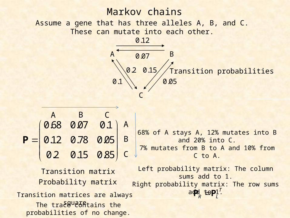
Markov chainsAssume a gene that has three alleles A, B, and C.

These can mutate into each other.

A B

C

0.1

0.2

0.05

0.15

0.07

0.12

0.68 0.07 0.1

0.12 0.78 0.05

0.2 0.15 0.85

P

Transition probabilities

Transition matrixProbability matrix

Left probability matrix: The column sums add to 1.Right probability matrix: The row sums add to 1.

Transition matrices are always square

The trace contains the probabilities of no change.

A B CA

B

C

68% of A stays A, 12% mutates into B and 20% into C.7% mutates from B to A and 10% from C to A.

TLR PP

Calculating probabilities

0.68 0.07 0.1

0.12 0.78 0.05

0.2 0.15 0.85

P

Probabilities to reach another state in the next step.

75.02585.0324.0

0935.06243.01852.0

1565.01172.04908.0

85.015.02.0

05.078.012.0

1.007.068.02

2P

Probabilities to reach another state in exactly two steps.

nn PP

The probability to reach any state in exactly n steps is given by

k k 1P U U

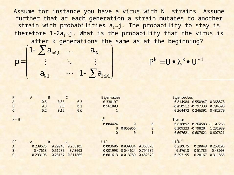
Assume for instance you have a virus with N strains. Assume further that at each generation a strain mutates to another strain with probabilities ai→j. The probability to stay is therefore

1-Σai→j. What is the probability that the virus is after k generations the same as at the beginning?

i 1,1 1N

N1 1,i 1

1 a a

p

a 1 a

k k 1P U U

P A B C Eigenvalues EigenvectorsA 0.5 0.05 0.3 0.338197 0.814984 0.550947 0.368878B 0.3 0.8 0.1 0.561803 -0.450512 -0.797338 0.794506C 0.2 0.15 0.6 1 -0.364472 0.246391 0.482379

k = 5 Lk Inverse0.004424 0 0 0.878092 0.264583 -1.107265

0 0.055966 0 0.109323 -0.798204 1.2310890 0 1 0.607621 0.607621 0.607621

PN A B C ULk ULkU-1

A 0.230675 0.20048 0.258105 0.003606 0.030834 0.368878 0.230675 0.20048 0.258105B 0.47613 0.51785 0.43003 -0.001993 -0.044624 0.794506 0.47613 0.51785 0.43003C 0.293195 0.28167 0.311865 -0.001613 0.013789 0.482379 0.293195 0.28167 0.311865

1 0

0.68 0.07 0.1 0.2 0.201

0.12 0.78 0.05 0.5 0.429

0.2 0.15 0.85 0.3 0.37

P PP

0.68 0.07 0.1

0.12 0.78 0.05

0.2 0.15 0.85

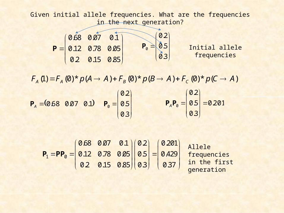
P Initial allele frequencies

Allele frequencies in the first generation

Given initial allele frequencies. What are the frequencies in the next generation?

)(*)0()(*)0()(*)0()1( ACpFABpFAApFF CBAA

3.0

5.0

2.0

0P

3.0

5.0

2.0

0P 1.007.068.0AP 201.0

3.0

5.0

2.0

0

PPA

A Markov chain is a process where step n depends only on the transition probabilities at step n-1 and

the realized values at step n.

A Marcov chain doesn’t have a memory.

n n 1 n 2 n 3 n 1 n n 1p(X i | X ,X ,X ...X ) p(X i | X )

Andrey Markov

(1856-1922)

02

012 )( PPPPPPPP 0PPP nn 1

0 0 n n

nX P X U U X

1 nn PPP

1)( nn n PPP Transition probabilities might change.

1 0

0.68 0.07 0.1 0.2 0.201

0.12 0.78 0.05 0.5 0.429

0.2 0.15 0.85 0.3 0.37

P PP

The model assumes constant transition probabilities.

Does our mutation process above reach in stable allele frequencies or do they change forever?

1 • n n nX X P X

Do we get stable frequencies?

n n nP X 1X (P 1I) X 0

Xn is a steady-state, stationary probability, or equilibrium vector.The associated eigenvalue is 1.

The equilibrium vector is

independent of the initial conditions.

The largest eigenvalue (principal eigenvalue) of every

probability matrix equals 1 and there is

an associated stationary

probability vector that defines the

equilibrium conditions (Perron-

Frobenius theorem).

P0.006159 0.260998 0.383385 0.312983 0.491399

0.23416 0.036019 0.314422 0.292022 0.3281440.101216 0.277682 0.087934 0.312887 0.0576070.245795 0.03226 0.115475 0.077524 0.008197

0.41267 0.39304 0.098784 0.004584 0.114652

Column sums 1 1 1 1 1

Eigenvalues Eigenvectors-0.49348933 0.676793 0.31531 0.049124 0.188368 0.5796-0.22284172 0.261813 -0.31217 -0.05106 0.002974 0.4894-0.10044735 -0.02386 0.714055 -0.81216 -0.60912 0.320660.139067327 -0.29236 -0.49289 0.451684 -0.29421 0.21635

1 -0.62238 -0.2243 0.362421 0.711985 0.52432

Eigenvalues and eigenvectors of probability matrices

Column sums of probability matrices are 1.Row sums might be higher.

The eigenvalues of probability matrices and their transposes are identical.

One of the eigenvalues of a probability matrix is 1.

P0.006159 0.260998 0 0.312983 0.491399

0.23416 0.036019 0 0.292022 0.3281440.101216 0.277682 1 0.312887 0.0576070.245795 0.03226 0 0.077524 0.008197

0.41267 0.39304 0 0.004584 0.114652

Column sums 1 1 1 1 1

Eigenvalues Eigenvectors-0.48893388 0 0.674168 0.386913 0.097599 0.274076 0-0.16647268 0 0.255996 -0.71988 -0.19397 0.230028 00.047131406 0 -0.00674 0.198906 0.254115 -0.88505 10.842629825 0 -0.29806 -0.30949 -0.74062 0.10075 0

1 0 -0.62536 0.443543 0.582882 0.280194 0

If one of the entries of P is 1, the matrix is called absorbing.

In this case the eigenvector of the largest eigenvalue contains only zeros and one 1.

Absorbing chains become monodominant by one

element.

To get frequencies the eigenvector has to be rescaled (normalized).

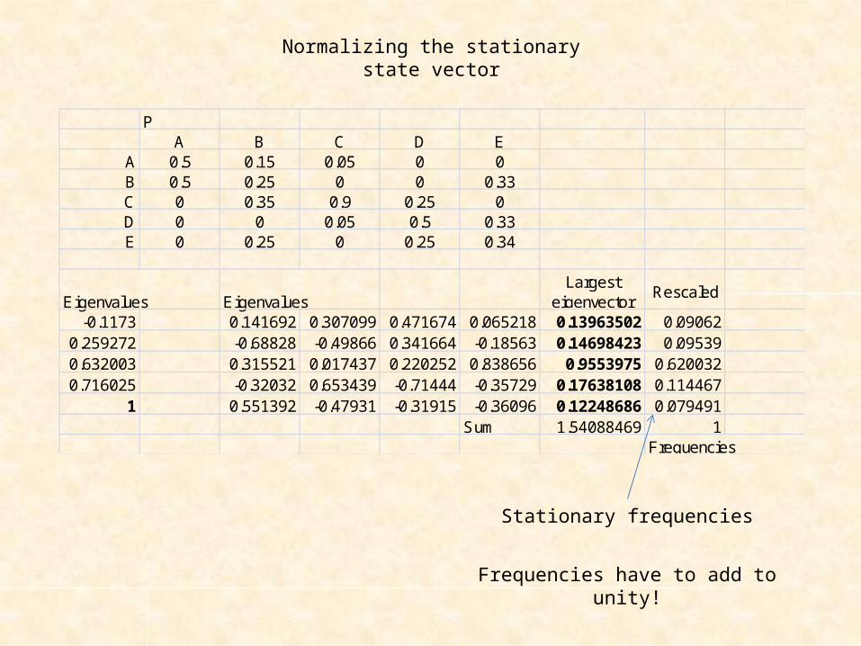
Normalizing the stationary state vector

PA B C D E

A 0.5 0.15 0.05 0 0B 0.5 0.25 0 0 0.33C 0 0.35 0.9 0.25 0D 0 0 0.05 0.5 0.33E 0 0.25 0 0.25 0.34

Eigenvalues EigenvaluesLargest

eigenvectorRescaled

-0.1173 0.141692 0.307099 0.471674 0.065218 0.13963502 0.090620.259272 -0.68828 -0.49866 0.341664 -0.18563 0.14698423 0.095390.632003 0.315521 0.017437 0.220252 0.838656 0.9553975 0.6200320.716025 -0.32032 0.653439 -0.71444 -0.35729 0.17638108 0.114467

1 0.551392 -0.47931 -0.31915 -0.36096 0.12248686 0.079491Sum 1.54088469 1

Frequencies

Frequencies have to add to unity!

Stationary frequencies

Final frequencies

The sum of the eigenvector entries have to be rescaled.

10 0

n nnX P X U U X

Eigenvalues3.14436E-23 0 0

0 2.46845E-15 00 0 1

Eigenvectors Inverse0.816257937 0.17364202 0.35099 1.005233 -0.07159 -0.38111-0.42522385 -0.77775251 0.385401 -0.2379 -0.93492 0.520064-0.39103409 0.604110489 0.853388 0.629018 0.629018 0.629018

Un UnU-1

2.56661E-23 4.28627E-16 0.35099 0.220779 0.220779 0.22078-1.3371E-23 -1.9198E-15 0.385401 0.242424 0.242424 0.24242-1.2296E-23 1.49122E-15 0.853388 0.536797 0.536797 0.5368

N=1000

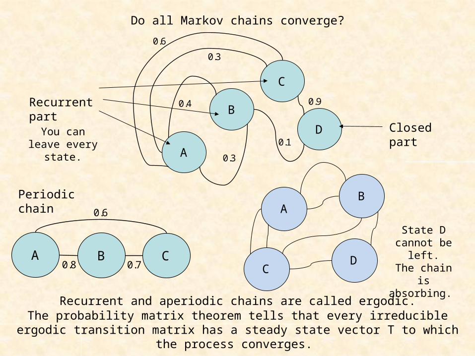
Do all Markov chains converge?

A

B

D

C

0.3

0.9

0.6

0.3

0.4

0.1

A B C

0.6

0.8 0.7

Closed part

Recurrent part

Periodic chain

Recurrent and aperiodic chains are called ergodic.

The probability matrix theorem tells that every irreducible ergodic transition matrix has a steady state vector T to which the process converges.

You can leave every state.

State D cannot be left.

The chain is absorbing.

A

CD

B

Absorbing chains

A

C D

BIt is impossible to leave state D

A chain is called absorbing if it containes states without exit.The other states are called transient.

Any absorbing Markov chain finally converges to the absorbing states.

Closed part

Absorbing part

A B C DA 0.5 0 0 0B 0.25 0.5 0 0C 0.25 0.25 0.5 0D 0 0.25 0.5 1

Eigenvalues Principal eigenvector0.5 0 0 0 00.5 0 0 0 00.5 0.707107 0.707107 0.707107 01 -0.70711 -0.70711 -0.70711 1

The time to reach the absorbing state

Home Bar

Assume a druncard going randomly through five streets. In the first street is his home, in the last a bar. At either home or bar he stays.

0.5 0.5 0.5

0.5 0.5 0.5

12/1000

002/100

02/102/10

002/100

0002/11

P

A B C D EA 1 0.5 0 0 0B 0 0 0.5 0 0C 0 0.5 0 0.5 0D 0 0 0.5 0 0E 0 0 0 0.5 1

Eigenvalues Principal eigenvectors-0.70711 0 0.143403 0.316228 0.544526 1 0

0 0 -0.48961 -0.63246 -0.31898 0 00.707107 0 0.692413 0 -0.4511 0 0

1 0 -0.48961 0.632456 -0.31898 0 01 0 0.143403 -0.31623 0.544526 0 1

A B C D EA 1 0.5 0 0 0B 0 0 0.5 0 0C 0 0.5 0 0.5 0D 0 0 0.5 0 0E 0 0 0 0.5 1

A E B C DA 1 0 0.5 0 0B 0 0 0 0.5 0C 0 0 0.5 0 0.5D 0 0 0 0.5 0E 0 1 0 0 0.5

A E B C DA 1 0 0.5 0 0E 0 1 0 0 0.5B 0 0 0 0.5 0C 0 0 0.5 0 0.5D 0 0 0 0.5 0

The canonical form

ttts

stsscanonical Q

RIP

0

We rearrange the transition matrix to have the s absorbing states in the upper left corner and the t

transient states in the lower right corner. We have four compartments

After n steps we have;

n

ttts

ss

n

ttts

stssn

Q

I

Q

RI

0

?

0P

The unknown matrix contains information about the frequencies to reach an absorbing

state from stateB, C, or D.

Transient part

n

ttts

ss

n

ttts

stssn

Q

I

Q

RI

0

?

0P

3

23

3

2

2

2

0

)(

0

0

)(

0

ttts

ss

ttts

stss

ttts

ss

ttts

stss

Q

QQIRI

Q

RI

Q

QIRI

Q

RI

P

P

nttts

in

istss

nttts

nss

n

ttts

stss

Q

QIRI

Q

QQQIRI

Q

RI

0

)(

0

)...(

0

1

0

123P

11

0

)()(lim

0lim

QIQI

Qn

i

in

nn Multiplication of probabilities gives ever smaller values

Simple geometric series

1)( QIRB tt

The entries nijof the matrix B contain the probabilities of ending in an absorbing state i

when started in state j.

1)( QIN tt

The entries nijof the fundamental matrix N of Q contain the expected numbers of time the process is in state i when started in state j.

11

1 )( tttttt IQIINt The sum of all rows of N gives the

expected number of times the chain is is state i (afterwards it falls to the absorbing

state).t is a column vector that gives the

expected number of steps (starting at state i) before the chain is absorbed.

1)( QIN tt

A B C D EA 1 0.5 0 0 0B 0 0 0.5 0 0C 0 0.5 0 0.5 0D 0 0 0.5 0 0E 0 0 0 0.5 1

A E B C DA 1 0 0.5 0 0B 0 0 0 0.5 0C 0 0 0.5 0 0.5D 0 0 0 0.5 0E 0 1 0 0 0.5

A E B C DA 1 0 0.5 0 0E 0 1 0 0 0.5B 0 0 0 0.5 0C 0 0 0.5 0 0.5D 0 0 0 0.5 0

The druncard’s walkQB C D

B 0 0.5 0C 0.5 0 0.5D 0 0.5 0

I I1 0 0 10 1 0 10 0 1 1

I-Q (I-Q)-1

B C D B C DB 1 -0.5 0 B B 1.5 1 0.5C -0.5 1 -0.5 C C 1 2 1D 0 -0.5 1 D D 0.5 1 1.5

RN NIB C D B 3

A 0.75 0.5 0.25 C 4E 0.25 0.5 0.75 D 3

The expected number of

steps to reach the absorbing

state.

The probability of reaching the

absorbing state from any of the transient states.

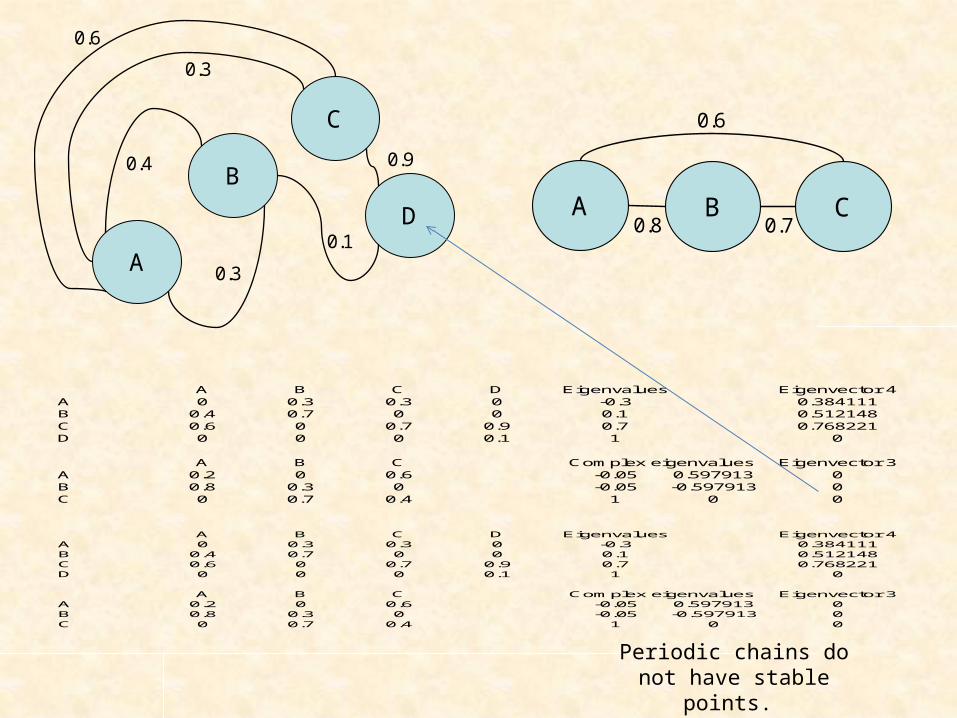
A B C D Eigenvalues Eigenvector 4A 0 0.3 0.3 0 -0.3 0.384111B 0.4 0.7 0 0 0.1 0.512148C 0.6 0 0.7 0.9 0.7 0.768221D 0 0 0 0.1 1 0

A B C Complex eigenvalues Eigenvector 3A 0.2 0 0.6 -0.05 0.597913 0B 0.8 0.3 0 -0.05 -0.597913 0C 0 0.7 0.4 1 0 0

A

B

D

C

0.3

0.9

0.6

0.3

0.4

0.1

A B C

0.6

0.8 0.7

Periodic chains do not have stable points.

A B C D Eigenvalues Eigenvector 4A 0 0.3 0.3 0 -0.3 0.384111B 0.4 0.7 0 0 0.1 0.512148C 0.6 0 0.7 0.9 0.7 0.768221D 0 0 0 0.1 1 0

A B C Complex eigenvalues Eigenvector 3A 0.2 0 0.6 -0.05 0.597913 0B 0.8 0.3 0 -0.05 -0.597913 0C 0 0.7 0.4 1 0 0

Expected return (recurrence) times

C

A

D

E

BIf we start at state D, how long does it take on average to

return to D?

iii ut

1

If u is the rescaled eigenvector of the probability matrix P, the expected return time tii of state i

back to i is given by the inverse of the ith element ui of the eigenvector u.

The rescaled eigenvector u of the probability matrix P gives the steady state frequencies to be in state i. 0.33

0.33

0.25

0.25

0.05

0.05

0.15

0.25

0.50

0.35

PA B C D E

A 0.5 0.25 0.05 0 0B 0.5 0.15 0 0 0.33C 0 0.35 0.9 0.25 0D 0 0 0.05 0.5 0.33E 0 0.25 0 0.25 0.34

Sum 1 1 1 1 1

Eigenvalue Eigenvector Rescaled 1/Rescaled-0.21 0.25 0.328 0.448 0.064 0.168 A 0.107644 9.2898550.212 -0.77 -0.37 0.197 0.235 0.146 B 0.093604 10.683330.655 0.295 -0.05 0.406 -0.88 0.951 C 0.608424 1.643590.732 -0.23 0.658 -0.67 0.262 0.176 D 0.11232 8.90278

1 0.456 -0.57 -0.38 0.317 0.122 E 0.078003 12.82Sum 1.563

In the long run it takes about

9 steps to return to D

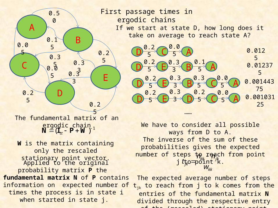
First passage times in ergodic chains

If we start at state D, how long does it take on average to reach state A?

C

A

D

E

B

0.33

0.33

0.25

0.25

0.05

0.05

0.15

0.25

0.50

0.35

1)( WPIN tt

Applied to the original probability matrix P the fundamental matrix N of P contains information on expected number of times the process is in

state i when started in state j.

D C A

D E B

D E B

A

C A

0.25 0.05

0.25 0.33 0.15

0.25 0.33 0.35 0.05

0.0125

0.012375

0.00144375

We have to consider all possible ways from D to A.The inverse of the sum of these probabilities gives the expected number of steps to reach from point j

to point k.

The fundamental matrix of an ergodic chain

D E D C A……

0.25 0.33 0.25 0.050.00103125

W is the matrix containing only the rescaled stationary point vector.

kk

jkkkjk w

nnt

The expected average number of steps tjk to reach from j to k comes from the entries of the fundamental matrix N

divided through the respective entry of the (rescaled) stationary point vector.

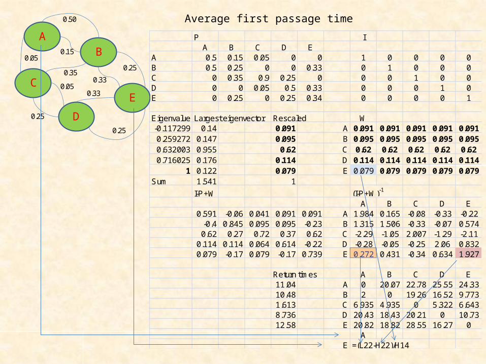
P IA B C D E

A 0.5 0.15 0.05 0 0 1 0 0 0 0B 0.5 0.25 0 0 0.33 0 1 0 0 0C 0 0.35 0.9 0.25 0 0 0 1 0 0D 0 0 0.05 0.5 0.33 0 0 0 1 0E 0 0.25 0 0.25 0.34 0 0 0 0 1

Eigenvalue Largest eigenvector Rescaled W-0.117299 0.14 0.091 A 0.091 0.091 0.091 0.091 0.0910.259272 0.147 0.095 B 0.095 0.095 0.095 0.095 0.0950.632003 0.955 0.62 C 0.62 0.62 0.62 0.62 0.620.716025 0.176 0.114 D 0.114 0.114 0.114 0.114 0.114

1 0.122 0.079 E 0.079 0.079 0.079 0.079 0.079Sum 1.541 1

I-P+W (I-P+W)-1

A B C D E0.591 -0.06 0.041 0.091 0.091 A 1.984 0.165 -0.08 -0.33 -0.22

-0.4 0.845 0.095 0.095 -0.23 B 1.315 1.506 -0.33 -0.07 0.5740.62 0.27 0.72 0.37 0.62 C -2.29 -1.05 2.007 -1.29 -2.11

0.114 0.114 0.064 0.614 -0.22 D -0.28 -0.05 -0.25 2.06 0.8320.079 -0.17 0.079 -0.17 0.739 E 0.272 0.431 -0.34 0.634 1.927

Return times A B C D E11.04 A 0 20.07 22.78 25.55 24.3310.48 B 2 0 19.26 16.52 9.7731.613 C 6.935 4.935 0 5.322 6.6438.736 D 20.43 18.43 20.21 0 10.7312.58 E 20.82 18.82 28.55 16.27 0

AE =(L22-H22)/H14

C

A

D

E

B

0.33

0.33

0.25

0.25

0.05

0.05

0.15

0.25

0.50

0.35

Average first passage time

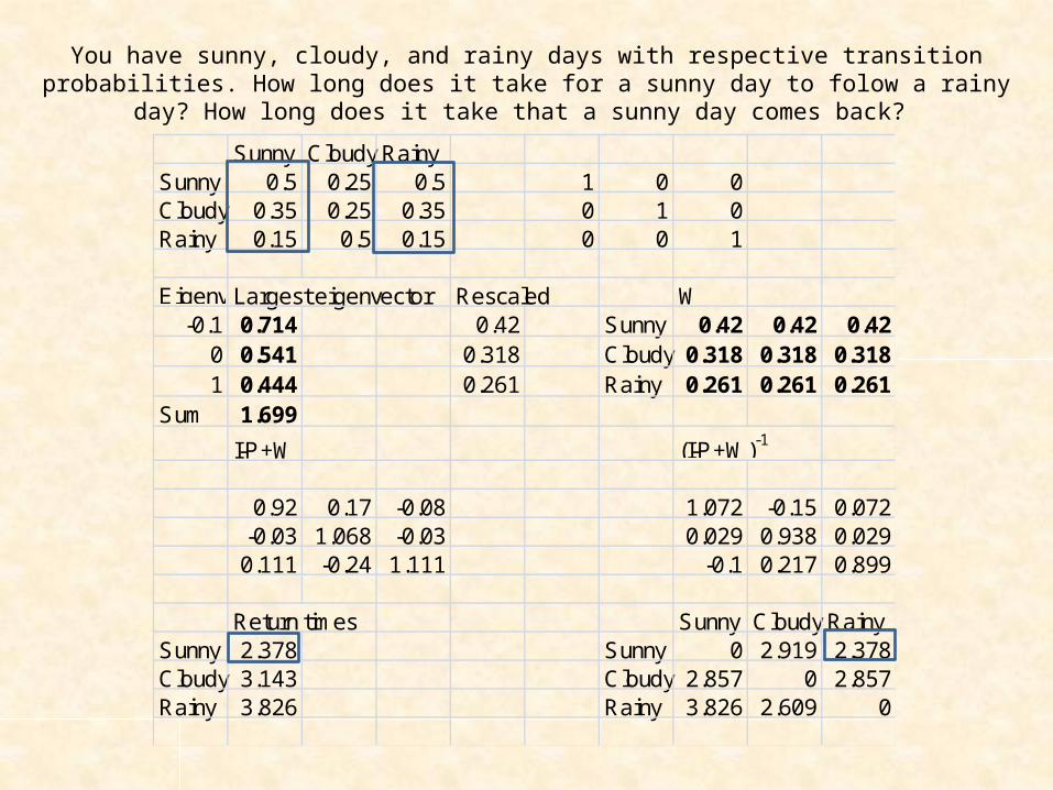
Sunny Cloudy RainySunny 0.5 0.25 0.5 1 0 0Cloudy 0.35 0.25 0.35 0 1 0Rainy 0.15 0.5 0.15 0 0 1

EigenvalueLargest eigenvector Rescaled W-0.1 0.714 0.42 Sunny 0.42 0.42 0.42

0 0.541 0.318 Cloudy 0.318 0.318 0.3181 0.444 0.261 Rainy 0.261 0.261 0.261

Sum 1.699

I-P+W (I-P+W)-1

0.92 0.17 -0.08 1.072 -0.15 0.072-0.03 1.068 -0.03 0.029 0.938 0.0290.111 -0.24 1.111 -0.1 0.217 0.899

Return times Sunny Cloudy RainySunny 2.378 Sunny 0 2.919 2.378Cloudy 3.143 Cloudy 2.857 0 2.857Rainy 3.826 Rainy 3.826 2.609 0

You have sunny, cloudy, and rainy days with respective transition probabilities. How long does it take for a sunny day to folow a rainy day? How long does it take that a sunny day comes back?

T→CTCA→GAG→C→GTG→C→AAACG

TTCA→GAGTGCCCT

Single substitution

Parallel substitution

Back substitution

Multiple substitution

Probabilities of DNA substitutionWe assume equal substitution probabilities. If the total probability for a substitution is p:

A T

C G

p

pp p

p

The probability that A mutates to T, C, or G isP¬A=p+p+pThe probability of no mutation ispA=1-3p

Independent events)()()( BpApBAp

Independent events

)()()( BpApBAp The probability that A mutates to T and C to G isPAC=(p)x(p)

p(A→T)+p(A→C)+p(A→G)+p(A→A) =1

The construction of evolutionary trees from DNA sequence data

pppp

pppp

pppp

pppp

P

31

31

31

31

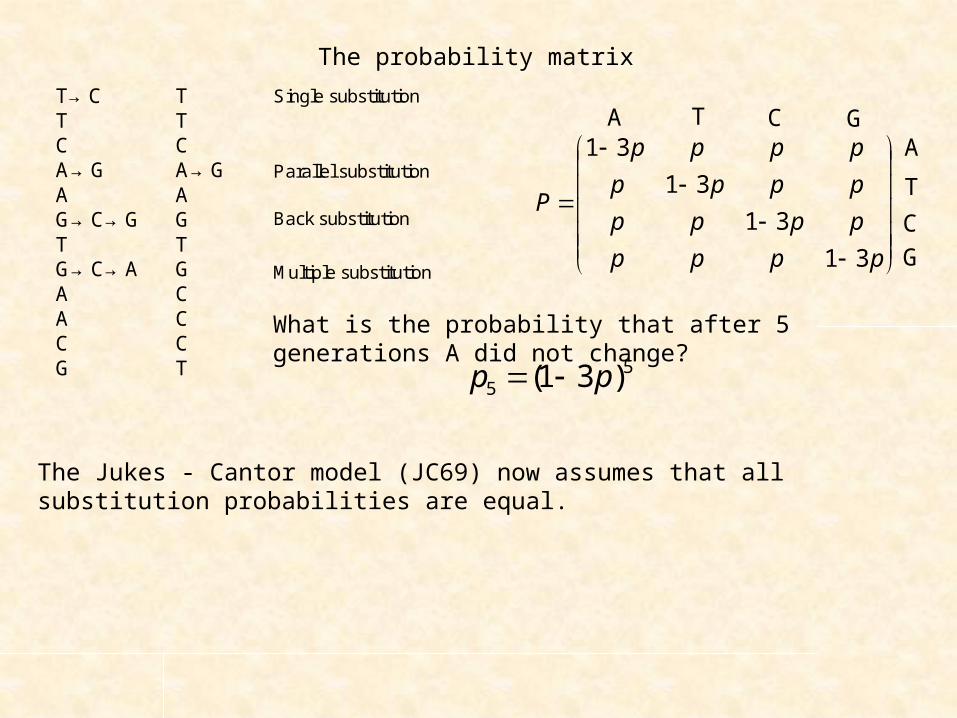
The probability matrix

T→CTCA→GAG→C→GTG→C→AAACG

TTCA→GAGTGCCCT

Single substitution

Parallel substitution

Back substitution

Multiple substitution

A T C GA

T

CG

What is the probability that after 5 generations A did not change?

55 )31( pp

The Jukes - Cantor model (JC69) now assumes that all substitution probabilities are equal.

Arrhenius model

The Jukes Cantor model assumes equal substitution probabilities within these 4 nucleotides.

Substitution probability after time t

tttt

tttt

tttt

tttt

eeee

eeee

eeee

eeee

P

4444

4444

4444

4444

43

41

41

41

41

41

41

41

41

41

43

41

41

41

41

41

41

41

41

41

43

41

41

41

41

41

41

41

41

41

43

41

Transition matrix

pppp

pppp

pppp

pppp

P

31

31

31

31

tPtP )0()(

tePtPtPdttdP )0()()()(

Substitution matrix

tA,T,G,C A

The probability that nothing changes is the zero term of the Poisson distribution

pteeGTCAP 4),,(

The probability of at least one substitution ispteeGTCAP 41)(

The probability to reach a nucleotide from any other is

)1(41

),,,( 4 pteACGTAP

The probability that a nucleotide doesn’t change after time t is

ptpt eeAGCTAAP 44

4

3

4

1))1(

4

1(31)|,,,(

Probability for a single difference

This is the mean time to get x different sites from a sequence of n nucleotides. It is also a measure of distance that dependents only on the number of

substitutions

ptpt eeGCTAAP 44

43

43

))1(41(3),,,(

What is the probability of n differences after time t?

xnpt

xptxnx ee

x

npp

x

ntxp

)

43

43(1

43

43

)1(),( 44

)

4

3

4

1ln)(

4

3

4

3lnln)1ln()(lnln),(ln 44 ptpt exnex

x

npxnpx

x

ntxp

nx

pt

34

1ln41

We use the principle of maximum likelihood and the Bernoulli distribution

0

0.05

0.1

0.15

0.2

0.25

0.3

0.35

0 1 2 3 4 5 6 7 8 9 10p

f(p)

1010( ) 0.2 0.8k kp k

k

GorillaPan paniscusPan troglodytesHomo sapiens

Homo neandertalensis

Time

nx

pt

34

1ln41

Divergence - number of substitutions

Phylogenetic trees are the basis of any systematic

classificaton