markov chain models for delinquency: transition matrix estimation
TRANSCRIPT
DMM Forecasting 1
Markov Chain Models for Delinquency:Transition Matrix Estimation and Forecasting
Scott D. Grimshaw 1∗, William P. Alexander 2
1 Department of Statistics, Brigham Young University, Provo, UT
2 Works Progress Analytics, Boise, ID
email: Scott D. Grimshaw ([email protected])
∗ Correspondence to Scott D. Grimshaw, Department of Statistics, Brigham Young Uni-
versity, Provo, UT 84602
KEY WORDS: Delinquency movement matrix, Dirichlet-Multinomial posterior, empirical
Bayes, loss forecasts, portfolio valuation, roll rates.
Abstract
A Markov chain is a natural probability model for accounts receivable. For example, accounts
that are “current” this month have a probability of moving next month into “current”,
“delinquent” or “paid-off” states. If the transition matrix of the Markov chain were known,
forecasts could be formed for future months for each state. This paper applies a Markov
chain model to subprime loans that appear neither homogeneous nor stationary. Innovative
estimation methods for the transition matrix are proposed. Bayes and empirical Bayes
estimators are derived where the population is divided into segments or subpopulations whose
transition matrices differ in some, but not all entries. Loan-level models for key transition
matrix entries can be constructed where loan-level covariates capture the nonstationarity of
the transition matrix. Prediction is illustrated on a $7 billion portfolio of subprime fixed first
mortgages and the forecasts show good agreement with actual balances in the delinquency
states.

DMM Forecasting 2
1 Introduction
Cyert et al. [1] proposed a discrete-time Markov chain model for estimating loss on accounts
receivable. The intuition and appeal behind a Markov chain model for accounts receivable
is that an account moves through different delinquency states each month. For example,
an account in the “current” state this month will be in the “current” state next month
if a payment is made by the due date and will be in the “30 days past due” state if no
payment is received. Another valuable feature is that the Markov chain model maintains
the progression and timing of events in the path from “current” to “loss.” For example, an
account in the “current” state doesn’t suddenly become a “loss.” Instead, an account must
progress monthly from the “current” state to the “30 days past due” state to the “90 days
past due” state and so on until foreclosure activities are completed and the collateral assets
are sold to pay the outstanding debt.
The transition matrix in the Markov chain represents the month-by-month movement
of loans between delinquency classifications or states. Barkman [2] observes the transition
matrix is often of interest as an accounting summary that evaluates loan quality or loan
collection practice. The matrix elements are commonly referred to as “roll-rates” since they
denote the probability that an account will move from one state to another in one month.
The transition matrix is sometimes referred to as the “roll-rate matrix” or the “delinquency
movement matrix” (DMM).
Another application of the Markov chain model in credit risk is introduced in Jarrow
et al. [3]. Institutional investors can use a continuous-time Markov chain model that in-
corporates credit ratings to assess the risk of structured finance securities. The states of
the Markov chain are the bond rating and the transition matrix reflects the likelihood of
maintaining a rating or migrating to another rating level. The transition matrix is called the
“migration matrix” in Gupton et al. [4] for CreditMetrics. The estimation of the continuous-
time Markov chain transition probabilities is introduced in Fleming [5] and more recently in
Monteiro et al. [6]. While the issue of correlation between issuers discussed in that research
may be applicable to a portfolio of mortgages, a mortgage is a simple accounts receivable
discrete-time Markov chain model with no arbitrage or hedging opportunities that require
more complicated model features.
The statistical problem of interest is to estimate the transition matrix using a sample of
observed monthly loan movements between delinquency states. The estimation is compli-
cated by the frequent observation in studies that the Markov chain is neither homogeneous

DMM Forecasting 3
nor stationary. Betancourt [7] concluded repayment for Freddie Mac data on prime mort-
gages was neither homogeneous nor stationary, and estimated transition matrices produce
poor forecasts. This paper proposes two innovative estimation methods for the transition
matrix based on two observations that improve forecasting precision.
First, it is common to divide a portfolio of loans into segments, where all loans within a
segment are similar and expected to have the same transition matrix. This practice may be
based on characteristics of the financial product or on data mining. For example, fixed-rate
loans are different in many ways from adjustable rate mortgage (ARM) loans so it seems
reasonable to assume they will have different transition matrices. Cyert and Thompson [8]
propose segments based on a credit score. However, there may not be enough observed
transitions within each segment to provide accurate estimates of all transition probabilities.
Second, it is reasonable to incorporate covariates that may change a few of the transition
probabilities for a given loan as it progresses through the repayment period. For example, the
data suggests that loans are more likely to remain current as they age. This nonstationarity
could be modeled with the covariate ‘number of months since last delinquency’ or ‘number of
months since origination.’ Other covariates that may model differences between loans over
the repayment period, are credit quality, repayment history, and loan age.
To address the first issue, segment transition probabilities are constructed by pooling
data from loans in the same segment and borrowing strength from data in other segments.
To address the second issue, using loan-level models for key transition probabilities allows
the incorporation of covariates that result in different transition probabilities for different
loans over the repayment period. Before describing the estimators, the notation and details
of using a Markov chain model to produce forecasts by delinquency state for a portfolio is
presented in Section 2. In Sections 3 and 4 Bayes and empirical Bayes estimates are described
for applications where the transition matrices for several segments differ in some, but not all
entries. Section 5 demonstrates how estimated loan-level models can be used in a few key
transition probabilities. Note that different covariates can be used in the different loan-level
models, as is demonstrated in an example where the “current” to “30 days past due” model
uses a repayment behavior covariate, but the “current’ to “paid” model uses the interest
rate covariate. The empirical Bayes estimates and loan-level models for current-to-30 days
past due and current-to-paid are applied to an example of forecasting a $7 billion portfolio
of subprime fixed first mortgages in Section 6. One of the important questions regarding the
applicability of the Markov chain model to forecasts is the effect of sampling variation in the
transition probability estimates on the forecasts, since forecasts are products of transition
DMM Forecasting 4
matrices. This question is addressed in Section 7 in a simulation study. This paper concludes
with a discussion of the value of the Markov chain model for delinquency and ideas for future
research in Section 8.
2 Using a Markov Chain Model to Produce Forecasts
of Outstanding Balance in Each Delinquency State
Let {Xn} denote a Markov chain where Xn is the delinquency state of a loan in month n.
Let π(n) denote the unconditional probability distribution of a loan in month n, and is a
vector whose entries correspond to the different Markov chain delinquency states. If the
delinquency state for month n is known, then πi(n) is a row vector with a one indicating this
month’s delinquency state for loan i and zeros elsewhere. The transition matrix moving from
month n to month n+ 1 of the Markov chain is denoted by P (n, n+ 1), a matrix containing
the probabilities of movement between delinquency states.
If the transition matrix is known, a forecast of the delinquency state probability distribu-
tion for next month can be formed given the previous month’s delinquency state probability
distribution. That is, for loan i, the delinquency state probability distribution of month
n + 1 is computed from πi(n + 1) = πi(n)Pi(n, n + 1) if πi(n) and Pi(n, n + 1) are known.
See Matis et al. [9] for an example of forecasting cotton yields using a Markov chain model
with changing transition matrix. Associated with loan i is an outstanding balance at month
n denoted by wi(n). The “one month ahead” forecast outstanding balance by delinquency
state of loan i is the vector wi(n+ 1) = wi(n) · πi(n+ 1).
Consider a simple example of a Markov chain model for a loan where the states are
defined as “current,” “delinquent,” “loss,” “paid.” Notice that if the transition matrix from
the 24th month since origination (n = 24) to the 25th month since origination (n = 25) was
Pi(24, 25) =
0.95 0.04 0.00 0.01
0.15 0.75 0.07 0.03
0.00 0.00 1.00 0.00
0.00 0.00 0.00 1.00
the matrix elements represent the probability of moving from a row state to a column state.
The value 0.04 in the first row second column is the probability of moving from “current”
this month to “delinquent” next month. Notice that the loss and paid state are absorbing

DMM Forecasting 5
states since eventually all loans terminate in one of these two states.
Suppose loan i is in the current state at n = 24 so that the delinquency state proba-
bility distribution is πi(24) =[
1 0 0 0]. The forecasted delinquency state probability
distribution of loan i for next month is
πi(25) = πi(24) · Pi(24, 25) =[
1 0 0 0]
0.95 0.04 0.00 0.01
0.15 0.75 0.07 0.03
0.00 0.00 1.00 0.00
0.00 0.00 0.00 1.00
=
[0.95 0.04 0.00 0.01
].
Suppose loan i was originated as a $50,000 30-year fixed-rate 12% APR (1% per month)
loan with a monthly payment of $514.30. If the borrower has made timely monthly payments
for 24 months, then this month (n = 24) the loan is in the current state with an outstanding
balance of $49,614.11. The “one month ahead” forecast outstanding balance by delinquency
state of loan i next month (n = 25) is
wi(25) = wi(24) · pi(25) = wi(24) · pi(24) · Pi(24, 25)
= ($49, 614.11) ·[
0.95 0.04 0.00 0.01]
=[
$47, 133.41 $1, 984.56 $0 $496.14].
While this forecast is on a specific loan, since the loan will be in only one of the delin-
quency states next month depending on what the borrower chooses to do, the forecast will
clearly be wrong. However, if a collection of loan-level forecasts (for example, in a portfolio
or a pool of securitized loans) is accumulated then the forecast balance by delinquency state
should be close to the actual balance by delinquency state. That is, if i = 1, . . . , N indexes
a portfolio of loans where each loan is ni months from origination this month, then the “one
month ahead” portfolio delinquency balance forecast is
N∑i=1
wi(ni + 1) =N∑i=1
wi(ni) · pi(ni + 1) =N∑i=1
wi(ni) · pi(ni) · Pi(ni, ni + 1).
If the Markov chain is stationary and homogeneous then all loans will have the same
DMM Forecasting 6
transition matrix and the calculation will not need to be performed on each loan. How-
ever, the emphasis of this paper is on applications in which loans are not homogeneous and
transition probabilities are known to change as the loan ages.
One appealing feature of the Markov chain model is that the forecast maintains the
timing of losses. This is demonstrated by the forecast of the delinquency state distribution
in two months. Notice that for loan i at month n, the “two month ahead” delinquency state
probability distribution is pi(n+ 2). Since
πi(n+ 2) = πi(n)Pi(n, n+ 2) = πi(n)Pi(n, n+ 1)Pi(n+ 1, n+ 2) = πi(n+ 1)Pi(n+ 1, n+ 2),
the “two month ahead” delinquency state probability distribution is the “one month ahead”
distribution multiplied by the transition matrix from n+1 to n+2. The “two month ahead”
forecast outstanding balance by delinquency state of loan i is wi(n+2) = w∗i (n+1)·pi(n+2),
where w∗i (n+ 1) differs from wi(n+ 1) because movement from a current state to a current
state or from a delinquent state to a current state next month indicates that loan payments
were made and the outstanding balance is reduced by one month’s principal payment.
Continuing the example of loan i that is in the current state at n = 24, the ‘two month
ahead’ delinquency state probability distribution is
πi(26) = πi(25)Pi(25, 26)
=[
0.95 0.04 0.00 0.01]
0.96 0.03 0.00 0.01
0.15 0.75 0.07 0.03
0.00 0.00 1.00 0.00
0.00 0.00 0.00 1.00
=
[0.9180 0.0585 0.0028 0.0207
]Notice Pi(25, 26) differs from Pi(24, 25) indicating that if the loan is still current at this point
in the loan age it is more likely to remain current and less likely to become delinquent.
To demonstrate the details of the outstanding balance, continue the example of loan
i, a $50,000 30-year fixed-rate 12% APR loan whose borrower has made timely monthly
payments for 24 months. While wi(24) = $49, 614.11, assuming timely payment last month
then w∗i (25) = $49, 595.94. This results in the ‘two month ahead’ forecast outstanding
balance by delinquency state is
wi(26) = w∗i (25) · pi(26)
DMM Forecasting 7
= ($49, 595.94) ·[
0.95 0.04 0.00 0.01]
0.96 0.03 0.00 0.01
0.15 0.75 0.07 0.03
0.00 0.00 1.00 0.00
0.00 0.00 0.00 1.00
= ($49, 595.94) ·
[0.9180 0.0585 0.0028 0.0207
]=
[$45, 529.08 $2, 901.36 $138.87 $1, 026.63
]It should be noted that there are other ways to handle the loan amortization component.
One is to recognize that delinquent loans will remain at the previous outstanding balance
plus interest. Another is to value loans based on the market value of a delinquent loan with a
given contract value and rate. This detail can be applied at the loan level before aggregating
the forecast for a collection of loans.
Throughout this simple example, only a few states are defined for the Markov chain.
In applications, the choice of the number and identity of the states is determined by the
monthly delinquency steps to loss and the desired reporting detail. Table 1 presents an
example transition matrix that demonstrates this point. In this example, loans are declared
loss after 120 days of delinquency. The ‘0’ state indicates current loans (borrower’s whose
monthly payment was received by the due date). The ‘30,’ ‘60,’ ‘90,’ and ‘120’ states are for
that are delinquent (1-30, 31-60, 61-90, 91-120 days past due). In this application, once a
loan becomes more than 150 days past due it is carefully analyzed to determine if it should be
declared a loss. The evaluation of a seriously delinquent loan may take several months while
loss mitigation and foreclosure options are pursued. There is no value to creating additional
monthly delinquency states just because the loan advances farther into delinquency. The
‘150+’ state contains all these seriously delinquent loans. Another interesting feature of the
states in this example is that the 0, 30, 60, 90, 120, 150+ states are duplicated, with one
collection falling under the ‘Never Bankrupt’ label and the other called ‘Bankrupt.’ This was
required since the lender required separate forecasts for borrowers who had filed personal
bankruptcy protection, and the model would allow borrowers to transition from the ‘Never
Bankrupt’ group to the ‘Bankrupt’ group.
Other definitions of states that may prove useful in other applications. For example, if
loans enter foreclosure proceedings after 60 days past due, choose the states: current, 30 days
past due, 60 days past due, enter foreclosure, 1, 2, 3+ mo in foreclosure, loss, paid. Another
example is when differences are known between current accounts based on the repayment
history, choose the states: 1, 2, 3, 4, 5, 6+ mo since last delinquency, delinquent, loss, paid.

DMM Forecasting 8
Embedded in the transition matrix in Table 1 is a wealth of information surrounding
both the quality of the loans and the practices of the loan collection or servicing. For
example the probabilities associated with the 0, 30 and 60 states reflect behavior of loans
in early stages of delinquency. While only 94.6% of loans stay current, aggressive action
on loans 30 days past due loans brings 29.5% of them back to current. It is interesting to
note that for borrowers in bankruptcy the principles are the same but the probabilities are
lower. Frequently the transition probabilities reflecting highly delinquent loans becoming
less delinquent is an accounting summary used to evaluate loss mitigation efforts such as
payment plans (in which the borrower agrees to make increased payments for a time to
bring the loan current). Also of interest are the probabilities that transition to the ‘Paid’
state. These are the single month mortality (SMM) used in modeling prepayment. As an
aside, the conditional prepayment rate (CPR) is the annualized SMM. Notice that current
loans have higher prepayment probability than delinquent loans, which is to be expected as
borrowers improve their credit by demonstrating payment on a subprime mortgage and then
exercising the opportunity to refinance to a less risky mortgage.
3 Bayesian Estimation
The goal of segmentation is to create groups in which some of the transition probabilities dif-
fer. While it may be easy to find segments with differences in a few transition probabilities,
it is difficult to identify segments with differences in all the entries of the transition matrix.
For those transition probabilities that are the same between segments, the segment estima-
tor is inefficient compared to the estimator based on the entire sample. Another practical
difficulty is that a segment must contain enough loans to estimate less frequent transition
probabilities like the “120 days past due” to “150 days past due” and “150 days past due” to
“current.” Some valuable segmentation schemes may not be possible because some segments
may have few observations for some transition probabilities.
Anderson and Goodman [10] show that the maximum likelihood estimator of the transi-
tion probabilities p(j, k) when the Markov chain is stationary is the fraction of the number of
observed transitions from state j to state k over the total number of observations beginning
in state j. There is confusion in the literature about whether the transition matrix should be
estimated by the movement of dollars or accounts between delinquency states. Cyert et al. [1]
and van Kuelen et al. [11] propose dollar estimation, while others use frequency estimation.
To demonstrate the distinction between dollar and frequency estimation, consider the data

DMM Forecasting 9
Tab
le1.
Exam
ple
Tra
nsi
tion
Mat
rix
for
anA
pplica
tion
wit
hM
ortg
age
Del
inquen
cy.
The
stat
esal
low
mon
thly
tran
siti
ons
todel
inquen
cyan
dpro
vid
eth
ere
quir
edre
por
ting
det
ail.
Tra
nsi
tion
pro
bab
ilit
ies
are
esti
mat
edfr
oma
sub-p
rim
ep
ortf
olio
offirs
tlien
fixed
-rat
e30
-yea
rm
ortg
ages
secu
red
by
resi
den
tial
real
esta
teas
sum
ing
stat
ionar
ity
(lik
ely
inap
pro
pri
ate)
.
Nev
erB
ankru
pt
Ban
kru
pt
TO
:0
3060
9012
015
0+0
3060
9012
015
0+L
oss
Pai
dFR
OM
:0
0.94
60.
042
0.00
30.
000
0.00
00.
000
0.00
20.
000
0.00
00.
000
0.00
00.
000
0.00
00.
006
300.
295
0.60
20.
079
0.00
60.
001
0.00
10.
001
0.00
30.
002
0.00
00.
000
0.00
00.
002
0.00
860
0.24
80.
249
0.30
00.
150
0.00
40.
004
0.00
10.
001
0.00
80.
016
0.00
00.
000
0.01
20.
007
900.
168
0.15
90.
136
0.25
50.
179
0.01
00.
001
0.01
10.
009
0.01
80.
017
0.00
10.
029
0.00
712
00.
055
0.01
40.
007
0.00
50.
749
0.02
10.
001
0.00
00.
000
0.00
00.
044
0.00
10.
100
0.00
315
0+0.
127
0.04
70.
024
0.01
30.
011
0.64
80.
001
0.00
00.
000
0.00
00.
000
0.02
00.
103
0.00
6B
K0
0.00
00.
000
0.00
00.
000
0.00
00.
000
0.92
00.
066
0.00
80.
001
0.00
00.
001
0.00
00.
004
BK
300.
000
0.00
00.
000
0.00
00.
000
0.00
00.
223
0.64
70.
096
0.00
80.
004
0.00
70.
010
0.00
5B
K60
0.00
00.
000
0.00
00.
000
0.00
00.
000
0.18
20.
148
0.45
00.
171
0.00
60.
017
0.02
10.
005
BK
900.
000
0.00
00.
000
0.00
00.
000
0.00
00.
119
0.11
70.
102
0.39
10.
206
0.03
20.
030
0.00
3B
K12
00.
000
0.00
00.
000
0.00
00.
000
0.00
00.
031
0.01
20.
003
0.01
00.
825
0.02
90.
087
0.00
3B
K15
0+0.
000
0.00
00.
000
0.00
00.
000
0.00
00.
071
0.02
30.
005
0.00
70.
015
0.80
30.
073
0.00
3L
oss
0.00
00.
000
0.00
00.
000
0.00
00.
000
0.00
00.
000
0.00
00.
000
0.00
00.
000
1.00
00.
000
Pai
d0.
000
0.00
00.
000
0.00
00.
000
0.00
00.
000
0.00
00.
000
0.00
00.
000
0.00
00.
000
1.00
0
DMM Forecasting 10
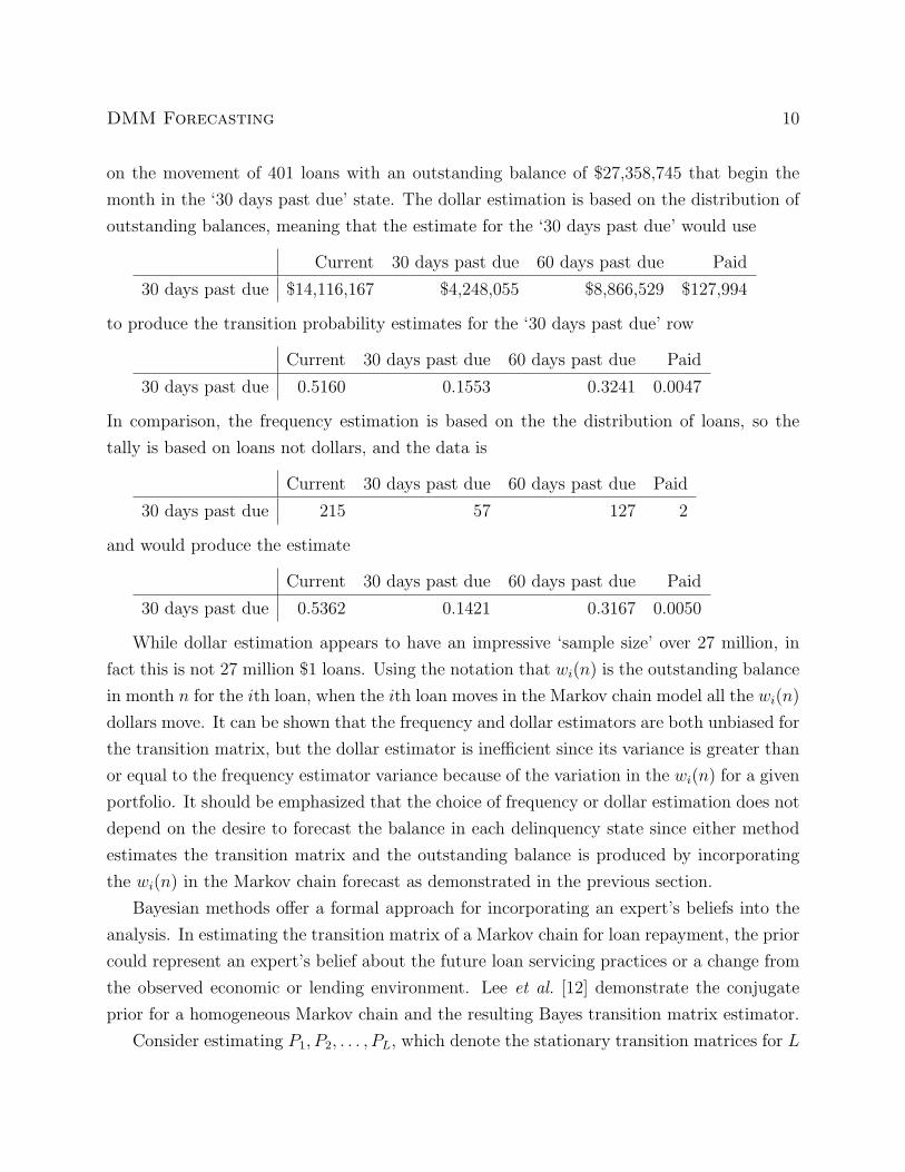
on the movement of 401 loans with an outstanding balance of $27,358,745 that begin the
month in the ‘30 days past due’ state. The dollar estimation is based on the distribution of
outstanding balances, meaning that the estimate for the ‘30 days past due’ would use
Current 30 days past due 60 days past due Paid
30 days past due $14,116,167 $4,248,055 $8,866,529 $127,994
to produce the transition probability estimates for the ‘30 days past due’ row
Current 30 days past due 60 days past due Paid
30 days past due 0.5160 0.1553 0.3241 0.0047
In comparison, the frequency estimation is based on the the distribution of loans, so the
tally is based on loans not dollars, and the data is
Current 30 days past due 60 days past due Paid
30 days past due 215 57 127 2
and would produce the estimate
Current 30 days past due 60 days past due Paid
30 days past due 0.5362 0.1421 0.3167 0.0050
While dollar estimation appears to have an impressive ‘sample size’ over 27 million, in
fact this is not 27 million $1 loans. Using the notation that wi(n) is the outstanding balance
in month n for the ith loan, when the ith loan moves in the Markov chain model all the wi(n)
dollars move. It can be shown that the frequency and dollar estimators are both unbiased for
the transition matrix, but the dollar estimator is inefficient since its variance is greater than
or equal to the frequency estimator variance because of the variation in the wi(n) for a given
portfolio. It should be emphasized that the choice of frequency or dollar estimation does not
depend on the desire to forecast the balance in each delinquency state since either method
estimates the transition matrix and the outstanding balance is produced by incorporating
the wi(n) in the Markov chain forecast as demonstrated in the previous section.
Bayesian methods offer a formal approach for incorporating an expert’s beliefs into the
analysis. In estimating the transition matrix of a Markov chain for loan repayment, the prior
could represent an expert’s belief about the future loan servicing practices or a change from
the observed economic or lending environment. Lee et al. [12] demonstrate the conjugate
prior for a homogeneous Markov chain and the resulting Bayes transition matrix estimator.
Consider estimating P1, P2, . . . , PL, which denote the stationary transition matrices for L

DMM Forecasting 11
segments. The data available to estimate the segment transition matrices are the observed
monthly account movements. Let f`(j, k) denote the number of accounts in segment ` that
started the month in state j and moved to state k the next month. Model the row vector of
observed monthly movements in segment `, denoted by
f`(j) = [f`(j, 1), f`(j, 2), . . . , f`(j,K)]
as a multinomial distribution. That is, the n`(j) =∑k f`(j, k) accounts that start the
month in state j move to the possible delinquency states according to the jth row of the `th
segment’s transition matrix, denoted by
p`(j) = [p`(j, 1), p`(j, 2), . . . , p`(j,K)],
where∑k p`(j, k) = 1. This model gives the likelihood function
L(f`(j) | p`(j)) =n`(j!)
f`(j, 1)! · · · f`(j,K)!p`(j, 1)f`(j,1) · · · p`(j,K)f`(j,K).
The conjugate prior for the multinomial is the Dirichlet distribution, whose parameters
are denoted by α(j) = [α(j, 1), α(j, 2), . . . , α(j, `)] with j indexing the different rows of the
transition matrix. Suppose p`(j) has prior distribution
π(p`(j) | α(j)) =Γ[M(j)]
Γ[α(j, 1)] · · ·Γ[α(j,K)]p`(j, 1)α(j,1)+1 · · · p`(j,K)α(j,K)+1,
where Γ(·) is the gamma function andM(j) =∑k α(j, k). This prior has the beta distribution
as a special case, corresponding to only two delinquency states when the binomial distribution
would be applicable.
A non-informative prior is nonsensical since transition probabilities are not equally likely
to occur. A reasonable practice for each row of the transition matrix is to allow the expert
to distribute M(j) loans according to their knowledge of loan quality and servicing. These
values are α(j, k). To demonstrate, Table 2 presents the α(j, k) assigned by an expert
for a subprime mortgage portfolio. In the top table, the expert believes most loans will
remain current, and of those that become delinquent the loan servicing is aggressive and
effective, with loans more likely to become less delinquent or prepay. In the bottom table,
the expert has represented repayment behavior in harsher economic times where borrowers
who become delinquent won’t have the resources to return to current and few refinancing
DMM Forecasting 12
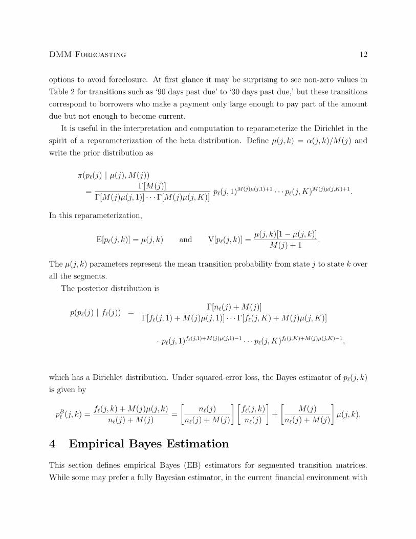
options to avoid foreclosure. At first glance it may be surprising to see non-zero values in
Table 2 for transitions such as ‘90 days past due’ to ‘30 days past due,’ but these transitions
correspond to borrowers who make a payment only large enough to pay part of the amount
due but not enough to become current.
It is useful in the interpretation and computation to reparameterize the Dirichlet in the
spirit of a reparameterization of the beta distribution. Define µ(j, k) = α(j, k)/M(j) and
write the prior distribution as
π(p`(j) | µ(j),M(j))
=Γ[M(j)]
Γ[M(j)µ(j, 1)] · · ·Γ[M(j)µ(j,K)]p`(j, 1)M(j)µ(j,1)+1 · · · p`(j,K)M(j)µ(j,K)+1.
In this reparameterization,
E[p`(j, k)] = µ(j, k) and V[p`(j, k)] =µ(j, k)[1− µ(j, k)]
M(j) + 1.
The µ(j, k) parameters represent the mean transition probability from state j to state k over
all the segments.
The posterior distribution is
p(p`(j) | f`(j)) =Γ[n`(j) +M(j)]
Γ[f`(j, 1) +M(j)µ(j, 1)] · · ·Γ[f`(j,K) +M(j)µ(j,K)]
· p`(j, 1)f`(j,1)+M(j)µ(j,1)−1 · · · p`(j,K)f`(j,K)+M(j)µ(j,K)−1,
which has a Dirichlet distribution. Under squared-error loss, the Bayes estimator of p`(j, k)
is given by
pB` (j, k) =f`(j, k) +M(j)µ(j, k)
n`(j) +M(j)=
[n`(j)
n`(j) +M(j)
] [f`(j, k)
n`(j)
]+
[M(j)
n`(j) +M(j)
]µ(j, k).
4 Empirical Bayes Estimation
This section defines empirical Bayes (EB) estimators for segmented transition matrices.
While some may prefer a fully Bayesian estimator, in the current financial environment with

DMM Forecasting 13
Table 2. Elicited Dirichlet α(j, k) Priors for the Transition Matrix for a Subprime MortgagePortfolio. The top table is an optimistic scenario with successful loan servicing where mostborrowers are believed to stick in delinquency states or get better and the timing of losses canbe managed. The bottom table is a pessimistic scenario where most borrowers proceed tohigher delinquency states and have few refinancing options to avoid foreclosure. The statesof the Markov chain model are: ‘0’ for current accounts; ‘30,’ ‘60,’ ‘90,’ ‘120’ denote 1 to30 days past due, 31 to 60 days past due, 61 to 90 days past due, 91 to 120 days past due,respectively; ‘150+’ denotes more than 150 days past due; ‘Loss’ denotes accounts where theaccount is closed due to nonpayment; and ‘Paid’ denotes accounts where the borrower paidoff the mortgage.
Days past due:TO: 0 30 60 90 120 150+ Loss Paid M(j)
FROM: 0 4,850,000 125,000 0 0 0 0 0 25,000 5,000,00030 2,500 6,400 1,000 0 0 0 0 100 10,00060 1,000 1,500 1,400 1,000 0 0 50 50 5,00090 525 375 600 720 600 0 150 30 3,000
120 100 40 40 100 1,400 100 200 20 2,000150+ 1,000 200 200 200 200 7,000 1,000 200 10,000Loss 0 0 0 0 0 0 1 0 1Paid 0 0 0 0 0 0 0 1 1
Days past due:TO: 0 30 60 90 120 150+ Loss Paid M(j)
FROM: 0 4,625,000 350,000 0 0 0 0 0 25,000 5,000,00030 1,000 2,500 6,500 0 0 0 0 50 10,00060 0 0 1,000 4,000 0 0 0 0 5,00090 0 0 0 300 2,700 0 0 0 3,000
120 0 0 0 0 100 1,900 0 0 2,000150+ 0 0 0 0 0 6,500 3,500 0 10,000Loss 0 0 0 0 0 0 1 0 1Paid 0 0 0 0 0 0 0 1 1

DMM Forecasting 14
Basel II requirements for model validation, it may appeal to auditors that the EB transition
matrix is a weighted average of the segment’s transition matrix and the grand mean transition
matrix estimated ignoring segmentation. Others may appreciate the argument in Efron’s
2004 Fisher lecture that empirical Bayes is a thoughtful compromise between frequentist
and Bayesian perspectives. Regardless of the motivation, one interesting feature of the EB
transition matrix estimator is that the weights are dictated by the value of segmentation in
the data.
If the Markov chain were stationary, the EB estimator derived in Billard and Meshkani
[13] for the transition matrix could be applied. However, Betancourt [7] found poor forecasts
on Freddie Mac prime mortgages using a homogeneous transition matrix and tried segment-
ing into five groups based on origination loan-to-value ratio (LTV) to improve the short-term
forecast performance. As discussed in the previous section, the data mining for segments that
improve forecasts is enticing but one would hardly expect to find segments whose transition
matrices differ for every possible transition. Instead, the exploration of segments needs to
maintain the properties of the Bayes estimator where truly different transition probabilities
between segments are well estimated but transition probabilities that are the same between
segments borrow strength across segments.
As described in Carlin and Louis [14], the basic empirical Bayes approach uses the ob-
served data to estimate the prior parameters. The parametric EB estimator uses the stan-
dard Bayes estimator where the prior parameters (µ(j),M(j)) are replaced by the estimates
(µ(j), M(j)), which maximizes the marginal likelihood L(f1(j), . . . , fL(j) | µ(j),M(j)), viewed
as a function of (µ(j),M(j)).
The marginal likelihood is
L(f1(j), . . . , fL(j) | µ(j),M(j))
=∫· · ·
∫f(f1(j), . . . , fL(j), p1(j), . . . , pL(j) | µ(j),M(j)) dp1(j) · · · dpL(j)
=∏`
∫f(f`(j), p`(j) | µ(j),M(j)) dp`(j)
=∏`
∫ n`(j)!
f`(j, 1)! · · · f`(j,K)!· Γ[M(j)]
Γ[M(j)µ(j, 1)] · · ·Γ[M(j)µ(j,K)]
· p`(j, 1)f`(j,1)+M(j)µ(j,1)−1 · · · p`(j,K)f`(j,K)+M(j)µ(j,K)−1dp`(j)
=∏`
n`(j)
f`(j, 1)! · · · f`(j,K)!· Γ[M(j)]
Γ[n`(j) +M(j)]

DMM Forecasting 15
· Γ[f`(j, 1) +M(j)µ(j, 1)]
Γ[M(j)µ(j, 1)]· · · Γ[f`(j,K) +M(j)µ(j,K)]
Γ[M(j)µ(j,K)].
When maximized and viewed as a function of (µ(j),M(j)) it is easier to consider the log
marginal likelihood, given by
lnL(µ(j),M(j)) =∑`
[lnn`(j)!− ln f`(j, 1)! · · · − ln f`(j,K)!]
+L ln(Γ[M(j)])−∑`
ln(Γ[n`(j) +M(j)])
+∑`
ln(Γ[f`(j, 1) +M(j)µ(j, 1)])− L ln(Γ[M(j)µ(j, 1)])
+ · · ·+∑`
ln(Γ[f`(j,K) +M(j)µ(j,K)])− L ln(Γ[M(j)µ(j,K)]).
The estimates (µ(j), M(j)), which maximize the log marginal likelihood, can be found using
non-linear optimization involving the digamma function for the derivative of the log of the
gamma function; however, it seems intuitive that p(j, k) =∑` f`(j, k)/
∑` n`(j) should be
extremely close to the optimal estimator µ(j, k), if it isn’t exactly equal. The parameter
µ(j, k) represents E[p`(j, k)], and p(j, k) is the proportion of accounts in all segments that
started the month in state j and moved to state k. Since p(j, k) is simple to compute, the
optimization simplifies from a nonlinear optimization over K + 1 space to a one-dimensional
optimization.
Conditional on µ(j, k) = p(j, k), the log marginal likelihood becomes
lnL(M(j)) =∑`
[lnn`(j)!− ln f`(j, 1)! · · · − ln f`(j,K)!]
+L ln(Γ[M(j)])−∑`
ln(Γ[n`(j) +M(j)])
+∑`
ln(Γ[f`(j, 1) +M(j)p(j, 1)])− L ln(Γ[M(j)p(j, 1)])
+ · · ·+∑`
ln(Γ[f`(j,K) +M(j)p(j,K)])− L ln(Γ[M(j)p(j,K)]).
If there is at least one state where p(j, k) > 0 and at least one segment ` such that
n`(j) ≥ 2 with at least one state with f`(j, k) ≥ 2 then the log marginal likelihood is
concave. The proof uses the digamma function, ψ = (x) = ddx
ln Γ(x) and the property of
the digamma function that ψ(x + 1) = ψ(x) + 1/x. Taking the derivative with respect to

DMM Forecasting 16
M(j) yields
d
d M(j)lnL(M(j))
= L · ψ[M(j)]−∑`
ψ[n`(j) +M(j)]
+∑`
ψ[f`(j, 1) +M(j)p(j, 1)] · p(j, 1)− L · ψ[M(j)p(j, 1)] · p(j, 1)
+ · · ·+∑`
ψ[f`(j,K) +M(j)p(j,K)] · p(j,K)− L · ψ[M(j)p(j,K)] · p(j,K)
=∑`
{ψ[M(j)]− ψ[n`(j) +M(j)]}
+∑k
∑`
p(j, k) · {ψ[f`(j, k) +M(j)p(j, k)]− ψ[M(j)p(j, k)]}
=∑`
{ψ[M(j)]− ψ[n`(j) +M(j)]}
+∑
{k: p(j,k)>0}
∑`
p(j, k) · {ψ[f`(j, k) +M(j)p(j, k)]− ψ[M(j)p(j, k)]}
=∑
{`: n`(j)=0}{ψ[M(j)]− ψ[n`(j) +M(j)]}
+∑
{`: n`(j)=1}{ψ[M(j)]− ψ[n`(j) +M(j)]}
+∑
{`: n`(j)≥2}{ψ[M(j)]− ψ[n`(j) +M(j)]}
+∑
{k: p(j,k)>0}
∑{`: f`(j,k)=0}
p(j, k) · {ψ[f`(j, k) +M(j)p(j, k)]− ψ[M(j)p(j, k)]}
+∑
{`: f`(j,k)=1}p(j, k) · {ψ[f`(j, k) +M(j)p(j, k)]− ψ[M(j)p(j, k)]}
+∑
{`: f`(j,k)≥2}p(j, k) · {ψ[f`(j, k) +M(j)p(j, k)]− ψ[M(j)p(j, k)]}
= 0
+∑
{`: n`(j)=1}
{ψ[M(j)]− ψ[M(j)]− 1
M(j)
}
+∑
{`: n`(j)≥2}
{ψ[M(j)]− ψ[M(j)]− 1
M(j)− 1
M(j) + 1
− · · · − 1
M(j) + n`(j)− 2− 1
M(j) + n`(j)− 1
}

DMM Forecasting 17
+∑
{k: p(j,k)>0}
{0
+∑
{`: f`(j,k)=1}p(j, k) ·
{ψ[M(j)p(j, k)] +
1
M(j)p(j, k)− ψ[M(j)p(j, k)]
}
+∑
{`: f`(j,k)≥2}p(j, k) ·
{ψ[M(j)p(j, k)]
+1
M(j)p(j, k)+
1
M(j)p(j, k) + 1+ · · ·
+1
f`(j, k) +M(j)p(j, k) − 2
+1
f`(j, k) +M(j)p(j, k) − 1
−ψ[M(j)p(j, k)]
}}
=∑
{`: n`(j)=1}
{− 1
M(j)
}
+∑
{`: n`(j)≥2}
{− 1
M(j)− 1
M(j) + 1
− · · · − 1
M(j) + n`(j)− 2− 1
M(j) + n`(j)− 1
}
+∑
{k: p(j,k)>0}
∑{`: f`(j,k)=1}
p(j, k) ·{
1
M(j)p(j, k)
}
+∑
{`: f`(j,k)≥2}p(j, k) ·
{1
M(j)p(j, k)+
1
M(j)p(j, k) + 1+ · · ·
+1
f`(j, k) +M(j)p(j, k) − 2
+1
f`(j, k) +M(j)p(j, k) − 1
}}
=∑
{k: p(j,k)>0}
∑{`: f`(j,k)=1}
{p(j, k) ·
[1
M(j)p(j, k)
]− 1
M(j)
}
+∑
{`: f`(j,k)≥2}
{p(j, k) ·
[1
M(j)p(j, k)
]− 1
M(j)
+p(j, k) ·[
1
M(j)p(j, k) + 1
]− 1
M(j) + 1+ · · ·
DMM Forecasting 18
+p(j, k) ·[
1
f`(j, k) +M(j)p(j, k) − 2
]− 1
f`(j, k) +M(j)− 2
+p(j, k) ·[
1
f`(j, k) +M(j)p(j, k) − 1
]− 1
f`(j, k) +M(j)− 1
− 1
f`(j, k) +M(j)− 1
f`(j, k) +M(j) + 1
− · · · − 1
M(j) + n`(j)− 2− 1
M(j) + n`(j)− 1
}}
=∑
{k: p(j,k)>0}
∑{`: f`(j,k)≥2}
{p(j, k) ·
[1
M(j)p(j, k) + 1
]− 1
M(j) + 1+ · · ·
+p(j, k) ·[
1
f`(j, k) +M(j)p(j, k) − 2
]− 1
f`(j, k) +M(j)− 2
+p(j, k) ·[
1
f`(j, k) +M(j)p(j, k) − 1
]− 1
f`(j, k) +M(j)− 1
− 1
f`(j, k) +M(j)− 1
f`(j, k) +M(j) + 1
− · · · − 1
M(j) + n`(j)− 2− 1
M(j) + n`(j)− 1
}}< 0
if there is at least one state k such that p(j, k) > 0 and at least one segment ` such that
n`(j) ≥ 2 with f`(j, k) ≥ 2.
A fairly efficient algorithm that takes advantage of the fact that the log marginal likeli-
hood is easy to evaluate, is to begin with a small value of M(j), such as one, and evaluate
lnL(M(j)). The search continues by incrementing M(j) by a small amount ∆, for example
one, evaluating lnL(M(j)) at the new value of M(j), and comparing the new value to the
previous value. When a value of M(j) decreases lnL(M(j)) the previous value is M(j).
After computing the estimates (µ(j), M(j)), the EB estimator of each transition proba-
bility in the jth row of the transition matrix for segment ` is given by
p`(j, k) =
[n`(j)
n`(j) + M(j)
] [f`(j, k)
n`(j)
]+
[M(j)
n`(j) + M(j)
]µ(j, k)
=
[n`(j)
n`(j) + M(j)
]p`(j, k) +
[M(j)
n`(j) + M(j)
]p(j, k).

DMM Forecasting 19
Notice this is a weighted average of the segment’s transition probability, denoted by p`(j, k) =
f`(j, k)/n`(j), and the grand mean transition probability, denoted by
p(j, k) =∑`
f`(j, k)/∑`
n`(j).
This weighted average estimator is very attractive. At one extreme is the estimator
p(j, k), which assumes all segments have the same value for the transition probability. If this
is true then p(j, k) is the most efficient estimator. At the other extreme is the segmented
estimator p(j, k), which assumes each segment may have a different value for the transition
probability. If this is true then the only unbiased estimator is p(j, k) since it is based solely
on the loans in a given segment.
Reality is likely to be somewhere in between these two extremes. For example, when a
segmentation is proposed for the entire transition matrix there will be some probabilities
that are different between the segments but there will also be many probabilities which are
the same for all segments. The EB transition matrix estimate chooses the weight based on
what the data in the segmentation indicates.
The weight in the segmented EB transition matrix estimator depends on the relative
size of M(j) and n`(j). When M(j) is small the variance between the segment transition
probabilities is large. This indicates that the segmentation provides evidence of differences in
the transition probabilities and the weight should favor the segment estimator p(j, k). When
M(j) is large the variance between the segment probabilities is small. When all the segment
transition probabilities in a row are identical, the conditional likelihood of M(j) is maximized
taking M(j) → ∞. The case M(j) → ∞ corresponds to the Dirichlet prior, yielding a
point mass at µ(j) = p(j). In addition to being an interesting diagnostic of a proposed
segmentation scheme, this result yields an upper bound for M(j) in the maximization of the
conditional likelihood. Choose as the upper bound a value of M(j) which makes the weight
on the p(j, k) component of the EB estimator sufficiently close to one.
One practical feature of the EB transition matrix estimator is that segmentations can be
explored with some protection against the practical worry that there won’t be enough data
to estimate some transition probabilities. The EB transition matrix estimator will return
the grand mean transition matrix estimate, estimated from the data in all segments, if a
segmentation is not useful or doesn’t have sufficient data. The Bayes Information Criterion
could be used to compare different segmentation schemes.
DMM Forecasting 20
5 Loan-Level Models
While many papers demonstrate the transition matrix is non-stationary, some of the estima-
tion approaches are quite extreme. Diggle et al. [15] describes a general approach to modeling
longitudinal categorical data as a Markov chain where the transition matrices P (n, n + 1)
have multinomial logistic models for each row with n as a covariate. Once a multinomial
model is introduced for each row of the transition matrix it is possible to include other
covariates. Smith and Lawrence [16] model all transition probabilities, but this extreme is
unnecessary for modeling mortgage repayment since only a few key transition probabilities
have non-constant probabilities. For example, the left panel of Figure 1 presents the pro-
portion of loans in a similar credit risk group that were “150+ days past due” in one month
and moved to “loss” the next month at different loan ages (months since origination). While
there is some variation, the scatter.smooth line indicates this particular transition proba-
bility appears constant over the life of a loan and it is acceptable to pool data regardless of
loan age to form an estimate. In contrast, the right panel of Figure 1 presents the proportion
of loans that were “current” in one month and moved to “30 days past due” the next month
for a similar credit risk group at different loan ages. The pattern is that the default risk
changes over loan lifetime, with the risk being very low after origination, reaching a peak and
then plateauing (or possibly declining for older loans). The “current” to “30 days past due”
transition probability changes over loan lifetime and there must be some way to include this
feature in Pi(n, n + 1). This section describes how loan-level models containing important
explanatory variables can be estimated for a few key transition probabilities and inserted
into the transition matrix.
Suppose Pi(n, n + 1) = P (xi; θ), meaning that changes in the transition matrix over n
as well as credit risk, loan characteristics, and collateral information on the ith loan are
represented by a set of explanatory variables. The extreme of estimating every row of the
transition matrix with a multinomial model, as done in Smith and Lawrence [16], has three
major concerns. First, not every transition probability merits modeling; for example, in the
row corresponding to loans “current” this month, while the probabilities of moving to “30
days past due” and moving to “prepay” should be modeled, there is no value to modeling
the “current” to “60 days past due” (a movement that appears to occur only on accounts
whose previous month’s payment check bounced) or the “current” to “loss” probabilities—
these calculations are unnecessary and would suffer the bias of overfitting even if a Bayesian
approach to estimation such as described in Sung et al. [17] and Healy and Engler [18].

DMM Forecasting 21
●
●
●
●●
●
●
●
●
●
●
●
●
0 20 40 60 80
0.0
0.1
0.2
0.3
0.4
0.5
150+ Days Past Due This Month Becoming Loss Next Month
Loan Age (months)
Pro
port
ion
●
●
●
●●
●●
●●
●
●
●
●
● ●
0 20 40 60 80
0.00
0.01
0.02
0.03
0.04
0.05
0.06
0.07
Current This Month Becoming 30 Days Past Due Next Month
Loan Age (months)P
ropo
rtio
n
Figure 1: The left panel is the proportion of loans 150+ days past due one month and lossthe next month over loan lifetime. This transition probability appears constant over time.The right panel is the proportion of loans current one month and 30 days past due the nextmonth over loan lifetime. This transition probability clearly changes over time.
Second, the explanatory variables may differ between transition probabilities; for example,
again considering the row for loans “current” this month, the explanatory variables for the
“current” to “30 days past due” probability are measures of credit and repayment history,
outstanding loan balance, and market value of the collateral, but the explanatory variables for
the “current” to “prepay” probability are an evaluation of the borrower’s interest rate and the
market interest rate available if the borrower were to refinance. Third, it is overly complicated
to model all the transition probabilities except in overly simple models; for example, the
simple model of Smith and Lawrence [16] requires 8 estimated transition probabilities, but
a Markov model with “current,” “30,” “60,” “90,” “120 or more days past due,” “loss,” and
“paid” states has 35 transition probabilities.
This paper proposes that the multinomial probability for any row of the transition matrix
can be estimated by a collection of binary logistic models using the results from Begg and
Gray [19]. Let p(j, k) for k = 1, . . . , K denote the probabilities of moving from the jth state
this month to the kth state next month. Writing the multinomial logistic for the jth row as
separate binary logistic models yields the collection
P[{state k next month} | {state j this month}]P[{state K next month} | {state j this month}]
= exp(x′j,kβj,k), k = 1, . . . , K − 1.

DMM Forecasting 22
To introduce a loan-level model for the transition probability p(j, k∗) with explanatory vari-
ables xj,k∗ , use a sample of loans that are in state j this month and move next month to
either state k∗ (Y = 1) or state K (Y = 0). The logistic model estimated from this sample
is denoted by x′k∗ βk∗ . If loan i has explanatory variables x∗j,k∗ , then
P[{state k∗} | {state j this month and state k∗ next month}
∪{state j this month and state K next month}]
=exp(x∗′j,k∗ βj,k∗)
1 + exp(x∗′j,k∗ βj,k∗).
It is important to stress that this is not the transition probability and more is required
than simply replacing p(j, k∗) with the prediction from this binary logistic prediction. With
respect to the multinomial logistic model for row j,
P[{state k∗ next month} | {state j this month}]P[{state K next month} | {state j this month}]
= exp(x∗′j,k∗ βj,k∗).
For any transition probabilities without a model, the binary logistic model is simply an
intercept. That is, suppose the transition from state j this month to state ko will use the
intercept only model. Then
P[{state ko next month} | {state j this month}]P[{state K next month} | {state j this month}]
= exp(βj,ko) =p(j, ko)
p(j,K),
where the estimated transition probability is denoted by p(j, k).
To combine all the binary logistic models (those with and without explanatory variables)
into the multinomial logistic model for the jth row, first compute the sum
C = 1 +∑k∗
exp(x∗′j,k∗ βj,k∗) +∑ko
p(j, ko)
p(j,K),
where the first sum is over all states that have loan-level models and the second sum is over
all states that are intercept only, but are not state K. Then, the elements of the jth row of

DMM Forecasting 23
the transition matrix are
p(j, k) =
p(j, k∗; xj,k∗ , βj,k∗) =exp(x∗′j,k∗ βj,k∗)
Cfor states with loan-level models
p(j, ko) =p(j, ko)/p(j,K)
Cfor states that are intercept only
p(j,K) =1
C
6 Example
Any company in the business of making loans will require a forecast of future cash flows
on their loans. The demands placed on the forecast are particularly heavy for companies
who securitize their loans. In essence, a group of loans is set aside in a trust. The cash
flow from these loans (principal and interest) is used to support bonds sold to investors. The
proper valuation of these bonds will depend critically on the amount and timing of losses and
prepayments over the life of the loans. Securitized loans form an unchanging pool. These
pools are small enough to expect noticeable variation in loss and prepayment rates even
within a stable environment.
The loans for this example are from a $7 billion portfolio in the subprime home equity
market. These borrowers generally have weaker or damaged credit, which prevents them from
qualifying for loans in the prime market. Not surprisingly, loss rates in the subprime sector
are greater than in the prime sector. These loans are fixed-rate, with first liens secured
by residential real estate originated between 1994 and 2002. Table 3 contains summary
statistics on these 97,124 loans. The proprietary credit score in Table 3 is a custom scorecard
that combines characteristics of the collateral and information from a recent credit report.
Characteristics about the collateral, such as the size of the lot and home, the year built, and a
general assessment of the quality of the home are used in the proprietary credit score, where
more valuable collateral motivates borrowers to make payments. Every four months a new
credit report is pulled for each loan from one of the bureaus. The counts of satisfactory trades,
inquiries the last six months, derogatories, and recent delinquencies, as well as information
from the different types of credit card outstanding balances and credit limits are useful
predictors of default. There is also some information about changes from the previous credit
report that are early predictors of changes in repayment behavior. Repayment behavior on
DMM Forecasting 24
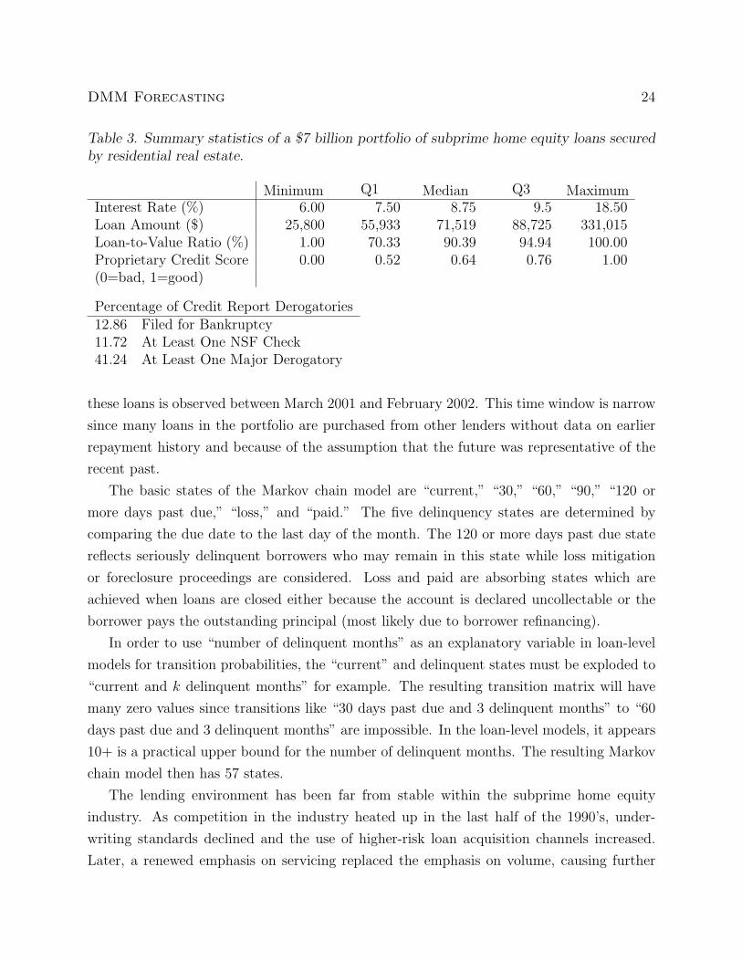
Table 3. Summary statistics of a $7 billion portfolio of subprime home equity loans securedby residential real estate.
Minimum Q1 Median Q3 MaximumInterest Rate (%) 6.00 7.50 8.75 9.5 18.50Loan Amount ($) 25,800 55,933 71,519 88,725 331,015Loan-to-Value Ratio (%) 1.00 70.33 90.39 94.94 100.00Proprietary Credit Score 0.00 0.52 0.64 0.76 1.00(0=bad, 1=good)
Percentage of Credit Report Derogatories12.86 Filed for Bankruptcy11.72 At Least One NSF Check41.24 At Least One Major Derogatory
these loans is observed between March 2001 and February 2002. This time window is narrow
since many loans in the portfolio are purchased from other lenders without data on earlier
repayment history and because of the assumption that the future was representative of the
recent past.
The basic states of the Markov chain model are “current,” “30,” “60,” “90,” “120 or
more days past due,” “loss,” and “paid.” The five delinquency states are determined by
comparing the due date to the last day of the month. The 120 or more days past due state
reflects seriously delinquent borrowers who may remain in this state while loss mitigation
or foreclosure proceedings are considered. Loss and paid are absorbing states which are
achieved when loans are closed either because the account is declared uncollectable or the
borrower pays the outstanding principal (most likely due to borrower refinancing).
In order to use “number of delinquent months” as an explanatory variable in loan-level
models for transition probabilities, the “current” and delinquent states must be exploded to
“current and k delinquent months” for example. The resulting transition matrix will have
many zero values since transitions like “30 days past due and 3 delinquent months” to “60
days past due and 3 delinquent months” are impossible. In the loan-level models, it appears
10+ is a practical upper bound for the number of delinquent months. The resulting Markov
chain model then has 57 states.
The lending environment has been far from stable within the subprime home equity
industry. As competition in the industry heated up in the last half of the 1990’s, under-
writing standards declined and the use of higher-risk loan acquisition channels increased.
Later, a renewed emphasis on servicing replaced the emphasis on volume, causing further

DMM Forecasting 25
non-stationarity in loss rates. One approach to modeling the changing subprime lending
environment is to estimate a different transition matrix for loans originating in each quarter.
That is, choose quarterly originations as the segmentation variable. This is problematic since
older loans have been observed longer than new loans and the rare transition probabilities
must have sufficient sample sizes for every segment. The EB transition matrix estimator is
appealing since it shrinks each segment transition probability toward the mean observed for
all loans. The amount of shrinkage depends on the sample size and the degree to which the
loans originated in a quarter differ from all subprime loans.
Figure 2 demonstrates how the EB estimates differ from the segment estimates. The
transition from “30” to “60 days past due” is frequently observed in subprime loans, and
the fact that these probabilities vary from 0.20 to 0.40 reflects the importance of early and
active management of delinquent subprime loans. The diameter of the circles centered at
each segment estimate in Figure 2 represents sample size, with large samples having large
circles. Notice that segments with large samples have little shrinkage, and the EB estimates
are very close to the segment estimates. The “90 days past due” to “current” event is
more unusual, since it represents loans that have progressed into serious delinquency but
then return to “current” through a large payment that covers the outstanding principle
and interest. The EB estimates demonstrate more shrinkage, particularly since the segment
estimates vary from 0.00 to 0.55 and the sample sizes within a segment are often small.
The next feature to incorporate into the transition matrix is the loan-level modeling of
a few critical transition probabilities. Because of the large number of loans in the “current”
row, precise transition probability estimates of the “30 days past due” and “paid” states
seem crucial to the forecast. There are some explanatory variables that would be common
to both models, but the mortgage repayment literature suggests default and refinance are
driven by different factors. The models presented here are simplifications and it is very likely
that many more explanatory variables would be included in the loan-level models.
First, consider the 1,014,362 observations on loans in the data set which were “current”
one month and moved to either “current” (Y = 0) or “30 days past due” (Y = 1) the next
month. A stratified sample is constructed for modeling containing all 7,626 observations
at Y = 1 and a random sample of 7,626 observations at Y = 0. The logistic regression
model is estimated with 90% of the stratified sample using the number of delinquent months
observed in repayment of this loan (ndlq), the loan-to-value percentage at origination (ltv),
the proprietary credit score (score), and the indicator variables for the origination year.
The estimated coefficients are given in Table 4. Figure 3 clarifies the piecewise linear ap-

DMM Forecasting 26
0.20 0.25 0.30 0.35 0.40 0.45
EB Estimate
0.20 0.25 0.30 0.35 0.40 0.45
Segment Estimate
●●● ●●● ●● ● ● ● ●●●
0.00 0.05 0.10 0.15 0.20 0.25 0.30 0.35
EB Estimate
0.00 0.05 0.10 0.15 0.20 0.25 0.30 0.35
Segment Estimate
● ●● ●● ●● ●●●●● ●●
Figure 2: Comparison of the empirical Bayes and segment estimates where segments arequarterly loan origination. The right panel is for the transition from 30 to 60 days past due.The left panel is for the transition from 90 days past due to current.
proximations for ndlq and ltv, as well as the differences over time in origination where
the increasing likelihood of default in recent origination years reflects the recent decline of
underwriting standards and use of higher-risk loan acquisition channels.
Two diagnostics of the quality of the model’s fit are the KS plot and the Decile plot for
the 10% holdout sample in Figure 4. The KS plot shows the separation of the empirical
distribution function of the estimated probabilities for the binary outcomes. The horizontal
axis is the corresponding percentile of the entire population. The distribution function of
the accounts that stayed “current” the next month is relatively linear since they represent
the majority of the population. A large distance between the two curves indicates a well-
performing model since the estimated probabilities for the two groups are well separated.
The KS score, the maximum difference between the two distribution functions, is 54, which is
respectable compared to delinquency models constructed in other credit scoring applications.
Credit scoring models can be measured by separating “goods” and “bads,” but prediction
is a requirement of a loan-level transition probability model. The Decile plot is constructed
by calculating the estimated probability of becoming “30 days past due” next month in the
holdout sample and grouping the probabilities into deciles. In each decile, the observed
proportion of loans moving from “current” this month to “30 days past due” next month
is computed. The Decile plot is the estimated probability and observed proportion for each
decile. The actual probabilities appear well predicted since the values fall closely on a unit

DMM Forecasting 27
●
●
●
● ●
0 2 4 6 8 10 12
1.5
2.0
2.5
3.0
ndlq
Par
tial L
ogis
tic
● ●
●
●
40 60 80 100
−0.
14−
0.12
−0.
10−
0.08
−0.
06−
0.04
−0.
020.
00
ltv
Par
tial L
ogis
tic●
●
●
●
●
●
●
●
1994 1995 1996 1997 1998 1999 2000 2001
−0.
4−
0.2
0.0
0.2
0.4
0.6
0.8
Origination Year
Par
tial L
ogis
tic
Figure 3: Piecewise linear approximation for the effect of number of delinquent monthsobserved in repayment of this loan (ndlq) and loan-to-value ratio at origination (ltv), aswell as the effect of origination year in the logistic model for loans “current” one month andeither “current” (Y = 0) or “30 days past due” (Y = 1) next month.
0 20 40 60 80 100
020
4060
8010
0
Percentile of Holdout Population
Per
cent
ile o
f Pop
ulat
ion
Moved to 30 Days Past Due
Stayed Current
KS = 54
●●●●
●●
●
●
●
●
0.00 0.01 0.02 0.03 0.04
0.00
0.01
0.02
0.03
0.04
Predicted Probability in Holdout Sample
Obs
erve
d P
ropo
rtio
n in
Hol
dout
Sam
ple
Figure 4: KS plot and Decile plot demonstrating holdout sample performance of the logisticmodel for loans “current” one month and either “current” (Y = 0) or “30 days past due”(Y = 1) next month. The KS plot indicates the separation in the population “goods” and“bads,” and the Decile plot indicates the prediction performance.

DMM Forecasting 28
Table 4. Estimated logistic regression coefficients for a loan-level estimate of the “current”to “30 days past due” transition probability. Both ndlq and ltv use a piecewise linearapproximation at the given knots to approximate the behavior of the gam model.
Coefficient Estimate seIntercept -4.8829 0.0000ndlq at 0 mo 1.5539 0.0783ndlq at 1 mo 2.3097 0.0726ndlq at 5 mo 2.7968 0.0677ndlq at 10+ mo 3.1895 0.0555ltv less than 50% -0.1377 0.0413ltv at 80% -0.1080 0.0705ltv at 100% 0.0000 0.0000score -4.6405 0.0873Originated 1994 0.0322 0.0748Originated 1995 -0.1200 0.0553Originated 1996 0.0000 0.0000Originated 1997 -0.0414 0.0467Originated 1998 0.1338 0.0446Originated 1999 0.2918 0.0450Originated 2000 0.5540 0.0506Originated 2001–02 0.7567 0.0855

DMM Forecasting 29
slope line through the origin. One feature of interest in the Decile plot is the large spread
of average probability from the highest to lowest decile, indicating a very high risk group in
the population for becoming delinquent.
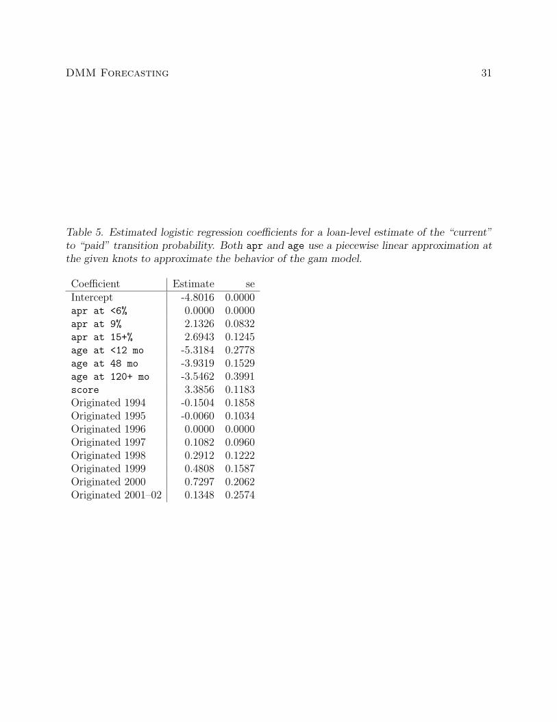
The “current” to “paid” loan-level model is based on a stratified sample of the available
1,015,008 observations where loans were “current” one month and moved to either “current”
(Y = 0) or “paid” (Y = 1) the next month. The stratified sample consists of all 8,272
observations at Y = 1 and a random sample of 8,272 observations at Y = 0. Table 5
contains the estimated logistic coefficients using 90% of the stratified sample. An important
explanatory variable in prepayment is interest rate (apr), which is included in addition
to number of months since loan origination (age), proprietary credit score (score), and
indicator variables for the origination year used in the previous model. Figure 5 provides
the partial logistic effects of the piecewise linear approximations for apr and age, as well as
the differences in origination over time where loans made recently are more likely to prepay.
Figure 6 contains the KS plot indicating typical separation for prepayment models and the
Decile plot indicating good prediction for a very small probability, both for the 10% holdout
sample.
The inclusion of exogenous covariates is intriguing because they have demonstrated im-
proved prediction in previously observed months. For example, the spread between the
mortgage interest rate and LIBOR would measure when the borrower had an incentive to
refinance to a lower rate. An improvement on the refinance incentive for subprime borrowers
was demonstrated in Alexander et al. [20] who used a covariate that measured the borrower’s
time-varying incentive to refinance when interest rates fall. The lender in their paper as-
signed each loan an internal grade at origination. The grade is based on loan-to-value ratio,
credit score, mortgage payment to income ratio, and mortgage payment history. Loans with
an A grade are the safest and a C- grade are the riskiest. In order to compute a borrower’s
incentive to refinance the assumption was that the borrower would refinance into the market
rate for the same grade. That is, if a borrower’s original loan was 15 basis points above the
average B+ rate for this lender then the refinance rate was computed to be 15 basis points
above the average B+ interest rate for this lender the current month. Another example
would be the time-varying state unemployment rate that would measure when a borrower is
likely to default.
The problem with including many exogenous covariates is that they are time-varying,
with the consequence that the Markov chain model requires future values of the exogenous
covariate for the prediction period to be provided. That is, while state unemployment rate

DMM Forecasting 30
●
●
● ●
6 8 10 12 14 16 18
0.0
0.5
1.0
1.5
2.0
2.5
apr
Par
tial L
ogis
tic
●
●
● ●
20 40 60 80 100 120 140
−5.
0−
4.5
−4.
0−
3.5
age
Par
tial L
ogis
tic
●
● ●
●
●
●
●
●
1994 1995 1996 1997 1998 1999 2000 2001
0.0
0.2
0.4
0.6
Origination Year
Par
tial L
ogis
tic
Figure 5: Piecewise linear approximation for the effect of interest rate (apr) and monthssince origination (age), as well as the effect of origination year in the logistic model for loans“current” one month and either “current” (Y = 0) or “paid” (Y = 1) next month.
0 20 40 60 80 100
020
4060
8010
0
Percentile of Holdout Population
Per
cent
ile o
f Pop
ulat
ion
Moved to Paid
Stayed Current
KS = 32
●
●
●●
●
●
●
●
●
●
0.000 0.005 0.010 0.015 0.020
0.00
00.
005
0.01
00.
015
0.02
0
Predicted Probability in Holdout Sample
Obs
erve
d P
ropo
rtio
n in
Hol
dout
Sam
ple
Figure 6: KS plot and Decile plot demonstrating holdout sample performance of the logisticmodel for loans “current” one month and either “current” (Y = 0) or “paid” (Y = 1) nextmonth. The KS plot indicates the separation in the population “goods” and “bads,” andthe Decile plot indicates the prediction performance.
DMM Forecasting 31
Table 5. Estimated logistic regression coefficients for a loan-level estimate of the “current”to “paid” transition probability. Both apr and age use a piecewise linear approximation atthe given knots to approximate the behavior of the gam model.
Coefficient Estimate seIntercept -4.8016 0.0000apr at <6% 0.0000 0.0000apr at 9% 2.1326 0.0832apr at 15+% 2.6943 0.1245age at <12 mo -5.3184 0.2778age at 48 mo -3.9319 0.1529age at 120+ mo -3.5462 0.3991score 3.3856 0.1183Originated 1994 -0.1504 0.1858Originated 1995 -0.0060 0.1034Originated 1996 0.0000 0.0000Originated 1997 0.1082 0.0960Originated 1998 0.2912 0.1222Originated 1999 0.4808 0.1587Originated 2000 0.7297 0.2062Originated 2001–02 0.1348 0.2574

DMM Forecasting 32
is known for the period where segments or loan-level models are estimated, these unknown
future values are now required inputs in the Markov chain model. One pragmatic approach
would be to use exogenous covariates with available forward curves or economist forecasts,
but this should be done cautiously since the forecasts have uncertainty that is not included
in the model.
It is certainly worth entertaining the idea of a few other loan-level models. The “30” to
“60 days past due” transition probability may be worth modeling if the loan servicer concen-
trated attention on early defaults. The “120+ days past due” to “loss” transition probability
could be modeled if loss mitigation and foreclosure proceedings played an important role in
determining the timing of losses. However, one must be conscious of the available sample
size to estimate these models, the performance of the available explanatory variables, and
the increasing complexity of the overall model.
One validation of the proposed model is to compare the forecast of the portfolio as
composed in March 2001 (the first month of the repayment data) to the actual values through
February 2002 (the last month of the repayment data). For each of the 97,124 loans, the
forecast is computed as detailed in Section 1 using the EB estimate and loan-level models
for the transition matrices. Figure 7 compares the actual and forecast balance for each state
of the Markov chain. There is good agreement in all states, particularly the “30 days past
due” and “paid” states, which demonstrates the value of the loan-level models. The worst
performances from the perspective of |y − y|/y are in the “90 days past due” and “loss”
states, where the difference is $3 million to $5 million relative to a $10 million to $16 million
balance.
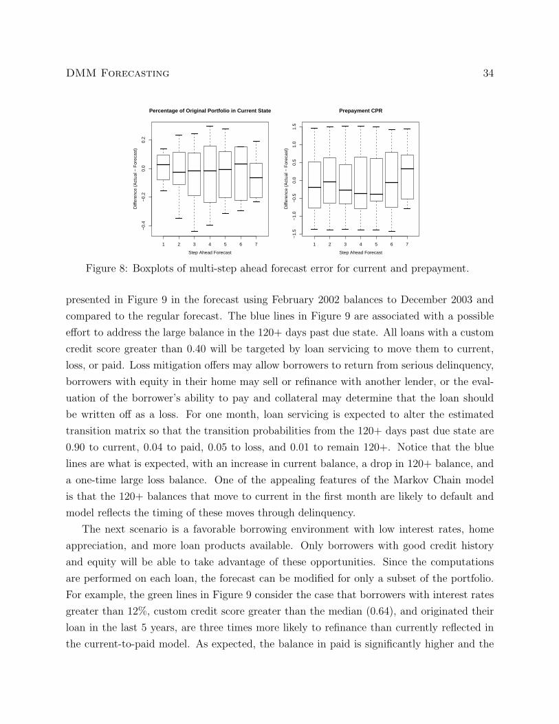
Another validation investigates the precision of multistep ahead forecasts. This is of
particular concern since the estimation focuses on the transition probabilities not the state
balances. Figure 8 contains boxplots of the multistep ahead forecast error for current and
prepayment. To compare current forecasts, consider the percentage of the original portfolio
balance in the current state k months ahead. The right panel of Figure 8 indicates the best
forecasts are one month ahead with the prediction variance increasing before leveling out
at about four months ahead. The comparison of prepayment is based on the conditional
prepayment rate (CPR), which measures prepayments as a percentage of the current out-
standing balance expressed as a compound annual rate. The left panel of Figure 8 indicates
equivalent forecasting of prepayments for all k month ahead forecasts.
Finally, to demonstrate a useful analytic feature of the model consider forecasts gener-
ated under possible loan servicing strategies or lending environments. Three examples are

DMM Forecasting 33
●
●
●
●
●
●
●
●
●
●
●
●
6.06.26.46.6
Cur
rent
$ Billion
Mar
Apr
May
Jun
Jul
Aug
Sep
Oct
Nov
Dec
Jan
Feb
2001
2002
●
●
●
●
●
●
●
●
●
●
●
●
Act
ual
For
ecas
t
●
●●
●
●
●
●
●
●●
●
●
464850525456
30 D
ays
Pas
t Due
$ Million
Mar
Apr
May
Jun
Jul
Aug
Sep
Oct
Nov
Dec
Jan
Feb
2001
2002
●
●●
●●
●●
●●
●●
●
●
●
●
●
●
●
●
●
●
●
●
●
2324252627
60 D
ays
Pas
t Due
$ Million
Mar
Apr
May
Jun
Jul
Aug
Sep
Oct
Nov
Dec
Jan
Feb
2001
2002
●
●
●
●●
●
●
●
●
●
●
●
●
●
●
●
●
●
●
●
●
●
●
●
12141618
90 D
ays
Pas
t Due
$ Million
Mar
Apr
May
Jun
Jul
Aug
Sep
Oct
Nov
Dec
Jan
Feb
2001
2002
●
●
●
●●
●●
●●
●●
●
●
●
●
●
●
●
●
●
●●
●●
105110115120125130135
120+
Day
s P
ast D
ue
$ Million
Mar
Apr
May
Jun
Jul
Aug
Sep
Oct
Nov
Dec
Jan
Feb
2001
2002
●
●
●
●
●
●
●
●
●
●
●
●
●
●●
●
●
●
●
●
●
●
●
10111213141516
Loss
$ Million
Mar
Apr
May
Jun
Jul
Aug
Sep
Oct
Nov
Dec
Jan
Feb
2001
2002
●
●
●
●
●
●
●●
●●
●
●
●
●
●
●
●
●
●
●
●
●
45505560
Pai
d
$ Million
Mar
Apr
May
Jun
Jul
Aug
Sep
Oct
Nov
Dec
Jan
Feb
2001
2002
●●
●●
●●
●●
●●
●
Fig
ure
7:A
ctual
and
For
ecas
tusi
ng
EB
tran
siti
onm
atri
xes
tim
ates
and
loan
-lev
elm
odel
sfo
r“c
urr
ent”
to“3
0day
spas
tdue”
and
“curr
ent”
to“p
aid”
tran
siti
onpro
bab
ilit
ies.
Val
idat
ion
isp
erfo
rmed
usi
ng
loan
son
the
book
sM
arch
2001
and
follow
edfo
r11
mon
ths.
While
“los
s”an
d“p
aid”
are
abso
rbin
gst
ates
,th
eplo
tis
ofea
chm
onth
’sad
dit
ion.
DMM Forecasting 34
1 2 3 4 5 6 7
−0.
4−
0.2
0.0
0.2
Percentage of Original Portfolio in Current State
Step Ahead Forecast
Diff
eren
ce (
Act
ual −
For
ecas
t)
1 2 3 4 5 6 7
−1.
5−
1.0
−0.
50.
00.
51.
01.
5
Prepayment CPR
Step Ahead Forecast
Diff
eren
ce (
Act
ual −
For
ecas
t)
Figure 8: Boxplots of multi-step ahead forecast error for current and prepayment.
presented in Figure 9 in the forecast using February 2002 balances to December 2003 and
compared to the regular forecast. The blue lines in Figure 9 are associated with a possible
effort to address the large balance in the 120+ days past due state. All loans with a custom
credit score greater than 0.40 will be targeted by loan servicing to move them to current,
loss, or paid. Loss mitigation offers may allow borrowers to return from serious delinquency,
borrowers with equity in their home may sell or refinance with another lender, or the eval-
uation of the borrower’s ability to pay and collateral may determine that the loan should
be written off as a loss. For one month, loan servicing is expected to alter the estimated
transition matrix so that the transition probabilities from the 120+ days past due state are
0.90 to current, 0.04 to paid, 0.05 to loss, and 0.01 to remain 120+. Notice that the blue
lines are what is expected, with an increase in current balance, a drop in 120+ balance, and
a one-time large loss balance. One of the appealing features of the Markov Chain model
is that the 120+ balances that move to current in the first month are likely to default and
model reflects the timing of these moves through delinquency.
The next scenario is a favorable borrowing environment with low interest rates, home
appreciation, and more loan products available. Only borrowers with good credit history
and equity will be able to take advantage of these opportunities. Since the computations
are performed on each loan, the forecast can be modified for only a subset of the portfolio.
For example, the green lines in Figure 9 consider the case that borrowers with interest rates
greater than 12%, custom credit score greater than the median (0.64), and originated their
loan in the last 5 years, are three times more likely to refinance than currently reflected in
the current-to-paid model. As expected, the balance in paid is significantly higher and the
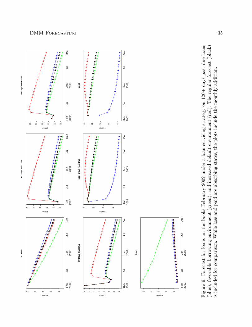
DMM Forecasting 35
●●
●●
●●
●●
●●
●●
●●
●●
●●
●●
●●
●
4.55.05.56.06.5
Cur
rent
$ Billion
●●
●●
●●
●●
●●
●●
●●
●●
●●
●●
●●
●
●
●
●
●
●
●
●
●
●
●
●
●
●
●
●
●
●
●
●
●
●
●
●
●
●●
●●
●●
●●
●●
●●
●●
●●
●●
●●
●●
●●
●●
●●
●●
●●
●●
●●
●●
●●
●●
●●
●
Feb
Jul
Jan
Jul
Dec
2002
2003
●
●●
●●
●●
●●
●●
●●
●●
●●
●●
●●
●●
505560657075
30 D
ays
Pas
t Due
$ Million
●
●●
●●
●●
●●
●●
●●
●●
●●
●●
●●
●●
●
●●
●●
●●
●●
●●
●●
●●
●●
●●
●●
●●
●
●
●●
●●
●●
●●
●●
●●
●●
●●
●●
●●
●
●
●●
●●
●●
●●
●●
●●
●●
●●
●●
●●
●●
Feb
Jul
Jan
Jul
Dec
2002
2003
●
●
●●
●●
●●
●●
●●
●●
●●
●●
●●
●●
●
222426283032
60 D
ays
Pas
t Due
$ Million
●
●
●●
●●
●●
●●
●●
●●
●●
●●
●●
●●
●
●
●
●●
●●
●●
●●
●●
●●
●●
●●
●●
●●
●
●
●
●
●●
●●
●●
●●
●●
●●
●●
●●
●●
●●
●
●
●●
●●
●●
●●
●●
●●
●●
●●
●●
●●
●
Feb
Jul
Jan
Jul
Dec
2002
2003
●
●
●
●●
●●
●●
●●
●●
●●
●●
●●
●●
●●
1213141516171819
90 D
ays
Pas
t Due
$ Million
●
●
●
●●
●●
●●
●●
●●
●●
●●
●●
●●
●●
●
●
●
●●
●●
●●
●●
●●
●●
●●
●●
●●
●●
●
●
●
●
●●
●●
●●
●●
●●
●●
●●
●●
●●
●
●
●
●
●●
●●
●●
●●
●●
●●
●●
●●
●●
●●
Feb
Jul
Jan
Jul
Dec
2002
2003
●●
●●
●●
●●
●●
●●
●●
●●
●●
●●
●●
●
6080100120
120+
Day
s P
ast D
ue
$ Million
●
●
●
●●
●●
●●
●●
●●
●●
●●
●●
●●
●●
●●
●●
●●
●●
●●
●●
●●
●●
●●
●●
●●
●
●●
●●
●●
●●
●●
●●
●●
●●
●●
●●
●●
●●
●●
●●
●●
●●
●●
●●
●●
●●
●●
●●
●●
Feb
Jul
Jan
Jul
Dec
2002
2003
●●
●●
●●
●●
●●
●●
●●
●●
●●
●●
●●
68101214
Loss
$ Million
●
●
●
●●
●●
●●
●●
●●
●●
●●
●●
●●
●
●●
●●
●●
●●
●●
●●
●●
●●
●●
●●
●●
●●
●●
●●
●●
●●
●●
●●
●●
●●
●●
●●
●●
●●
●●
●●
●●
●●
●●
●●
●●
●●
●●
Feb
Jul
Jan
Jul
Dec
2002
2003
●●
●●
●●
●●
●●
●●
●●
●●
●●
●●
●●
60708090100
Pai
d
$ Million
●●
●●
●●
●●
●●
●●
●●
●●
●●
●●
●●
●
●
●
●
●
●
●
●
●●
●●
●●
●●
●●
●●
●●
●●
●●
●●
●●
●●
●●
●●
●●
●●
●●
●●
●●
●●
●●
●●
●●
●●
●●
●●
●●
●●
●●
Feb
Jul
Jan
Jul
Dec
2002
2003
Fig
ure
9:F
orec
ast
for
loan
son
the
book
sF
ebru
ary
2002
under
alo
anse
rvic
ing
stra
tegy
on12
0+day
spas
tdue
loan
s(b
lue)
,fa
vora
ble
bor
row
ing
envir
onm
ent
(gre
en),
and
incr
ease
ddef
ault
envir
onm
ent
(red
).T
he
regu
lar
fore
cast
(bla
ck)
isin
cluded
for
com
par
ison
.W
hile
loss
and
pai
dar
eab
sorb
ing
stat
es,
the
plo
tsin
clude
the
mon
thly
addit
ion.
DMM Forecasting 36
balance of current loans is much lower. One interesting feature is that the paid balance is
declining over time instead of increasing as shown in the regular forecast. This is because
borrowers who can will refinance quickly in this borrowing environment leaving a smaller
portfolio for later months.
Finally, consider the case where rising interest rates, declining home prices, and a slow
economy result in more defaults. The red lines indicate forecasts if borrowers with a delin-
quency in loan repayment, a loan-to-value ration greater than 80%, and custom credit score
less than the upper quartile (0.76) are 50% more likely to default than the current-to-30
model. As expected, ultimately there is an increase in loss but the Markov Chain model
maintains the timing that those losses won’t be observed until the March 2002 increase in
30 days past due works through the 60, 90, and 120+ states.
7 Simulation Study
The sampling distributions of the estimated transition probabilities are well known, but the
practical importance of the Markov chain model is in its predictions. A simulation study
based on the subprime example in the previous section investigates how sampling variation
in transition probability estimates affects prediction precision. Consider a homogeneous
stationary Markov chain with states “current,” “30,” “60,” “90,” “120+ days past due,”
“loss,” and “paid.” For all simulations, the transition matrix is given in Table 6 and is
the mean transition matrix from the subprime example given in Section 6. The simulation
investigates the first observation month, the number of months in which loan movements are
observed, and the number of loans in the initial portfolio. The results of 10,000 replications
for each simulation are presented in Table 7.
The most important question is the performance of the estimator in future forecasts.
After estimating the transition matrix, forecasts 12, 24, 36, and 48 months ahead of the
number of loans in each state are compared to the simulated path using the true transition
matrix. As expected, the median absolute deviation (MAD) comparing the actual and
predicted proportion of loans in non-absorbing states usually increases as the forecast horizon
increases. The exceptions are transitions to absorbing states, which may be due to smaller
proportions of loans moving to these states further into the future.
One interesting feature of estimating the transition matrix is that the individual transition
sample size can not be selected, but the movements from a beginning portfolio must be
observed. The upper and lower portions of Table 7 compare different numbers of loans

DMM Forecasting 37
Table 6. Transition matrix for simulation study. The homogeneous Markov chain has statesstates “current,” “30,” “60,” “90,” “120+ days past due,” “loss,” and “paid.” and wasconstructed from the mean transition matrix from the subprime example given in Section6.
P =
0.983 0.008 0.001 0.000 0.000 0.000 0.0080.532 0.116 0.333 0.004 0.003 0.002 0.0100.279 0.019 0.052 0.481 0.152 0.010 0.0070.161 0.005 0.012 0.043 0.748 0.025 0.0060.053 0.001 0.001 0.001 0.834 0.108 0.0020.000 0.000 0.000 0.000 0.000 1.000 0.0000.000 0.000 0.000 0.000 0.000 0.000 1.000
at the beginning of the Markov chain. Clearly more loans result in smaller error since the
transition probabilities as a whole become better estimated with more data, even if particular
transitions have few observations.
A common question in applying the Markov chain model for delinquency is the trade-
off between a wide window of monthly data to improve estimation and a narrow window of
monthly data to represent current loan servicing practice. The simulation indicates that more
data is always better, but six months of data results in adequate prediction performance.
The final comparison is between scenarios where loans are observed from the beginning
compared to scenarios where loans are observed after 36 months. That is, can the first few
months be used to estimate the transition matrix or does the model require a few months for
the loans to distribute among the states? The MAD indicates forecasts are better when loans
have been in the Markov chain a few months, but forecasts are acceptable when observing
a large portfolio of loans the first six months to estimate transition probabilities. However,
Figure 10 indicates that the prediction error is not symmetric in the forecasts based on early
observations. It appears underestimating the current state and overestimating the delinquent
states is quite common.
8 Conclusion
This paper proposes innovative approaches to estimating the transition matrix for a Markov
chain model for accounts receivable. When applied to forecasting balances in delinquency
states for a portfolio of subprime loans, the transition matrix is unknown and must be es-
timated from observed monthly loan transitions. When a portfolio consists of loans from

DMM Forecasting 38
Table 7. Median absolute deviation of 12, 24, 36, and 48 months ahead forecasts of proportionof loans in non-absorbing states at last observed month that are “current,” “90+ days pastdue,” “loss,” and “paid” for the simulation study. While “loss” and “paid” are absorbingstates, the deviation is computed from the monthly addition.
1,000 Loans Begin in Current State
First Observed MonthMonths 1 36Observed 12 24 36 48 12 24 36 486 Current 0.824 1.067 1.150 1.174 0.677 0.747 0.777 0.815
90 + 0.743 0.950 1.012 1.034 0.533 0.606 0.620 0.647Loss 0.105 0.105 0.102 0.091 0.113 0.106 0.100 0.092Paid 0.197 0.182 0.164 0.161 0.228 0.213 0.199 0.193
12 Current 0.545 0.613 0.646 0.664 0.596 0.646 0.685 0.70290 + 0.442 0.500 0.529 0.539 0.463 0.503 0.530 0.545Loss 0.094 0.092 0.091 0.089 0.126 0.117 0.106 0.096Paid 0.197 0.182 0.172 0.166 0.229 0.213 0.208 0.190
10,000 Loans Begin in Current State
First Observed MonthMonths 1 36Observed 12 24 36 48 12 24 36 486 Current 0.246 0.300 0.324 0.319 0.216 0.235 0.201 0.205
90 + 0.218 0.280 0.297 0.296 0.169 0.188 0.191 0.200Loss 0.033 0.032 0.031 0.029 0.034 0.032 0.031 0.029Paid 0.061 0.057 0.053 0.051 0.072 0.067 0.063 0.059
12 Current 0.172 0.190 0.201 0.205 0.187 0.208 0.297 0.29690 + 0.138 0.158 0.164 0.169 0.147 0.163 0.168 0.172Loss 0.029 0.028 0.026 0.024 0.035 0.032 0.030 0.028Paid 0.062 0.058 0.054 0.051 0.072 0.069 0.064 0.060

DMM Forecasting 39
12mo 24mo 36mo 48mo
−5
05
10
Current
12mo 24mo 36mo 48mo
−10
−5
05
90+ Delq
12mo 24mo 36mo 48mo
−0.
4−
0.2
0.0
0.2
0.4
Loss
12mo 24mo 36mo 48mo
−1.
0−
0.5
0.0
0.5
1.0
Paid
12mo 24mo 36mo 48mo
−5
05
10
Current
12mo 24mo 36mo 48mo
−10
−5
05
90+ Delq
12mo 24mo 36mo 48mo
−0.
4−
0.2
0.0
0.2
0.4
Loss
12mo 24mo 36mo 48mo
−1.
0−
0.5
0.0
0.5
1.0
Paid
Figure 10: Boxplots of prediction error for 12, 24, 36, and 48-month ahead forecasts ofproportion of loans in non-absorbing states at last observed month that are current, 90+days past due, loss, and paid for simulation study with 1,000 loans beginning in the currentstate and observed for 6 months. While loss and paid are absorbing states, the deviation iscomputed from the monthly addition.

DMM Forecasting 40
different segments, Bayes and empirical Bayes estimators allow different estimates for those
transition probabilities that differ between segments but borrow strength in estimating tran-
sition probabilites that are the same between segments. Additional covariates can be used to
construct loan-level models for a few key transition probabilities that reflect differences over
time and credit quality. The case study on a $7 billion securitized portfolio of subprime home
equity loans demonstrates estimated transition matrices and resulting forecasts. Differences
in underwriting standards over time can be modeled using empirical Bayes estimators. More
precise predictions for the “current” to “30 days past due” and “paid” transitions can be
made by incorporating past repayment behavior, interest rate, and home equity as covari-
ates in loan-level models. A simulation study indicates the estimated transition matrix can
produce reasonable predictions. Some of the important elements of good prediction include
the number of loans observed, the number of months observed, and the first observation of
the Markov chain.
Like any model using historical data to make forecasts, the Markov chain model would
not have forecasted the rapid decline in subprime mortgage valuations when the data showed
servicing was effective and borrowers had equity in their homes that could be used to avoid
delinquency. One can speculate that a Bayes estimator of the transition matrix using a prior
as shown in the pessimistic scenario in Table 2 foretelling a change in borrower repayment
that dominated the historical data would have indicated the possibility of a rapid change to
the high subprime default rates observed in the last year. More realistically, efficient use of
the data in transition probability estimation would provide accurate revised forecasts using
only a few months of data. That is, even with only three or four months of repayment be-
havior data during the current recession, segmented transition matrices could be estimated
and loan-level models for a few key transition probabilities could be constructed with useful
covariates. These estimates applied within the mechanics of the Markov chain model would
produce revised short-term forecasts that would be far superior to those still based on pre-
dominantly older data or models that needed longer horizon data before a revised forecast
could be constructed.
ACKNOWLEDGEMENTS
We are grateful to the Editor, Associate Editor, and referees of Applied Stochastic Models
in Business and Industry for helpful comments on an earlier draft and for suggestions that
substantially improved the paper.

DMM Forecasting 41
References
1. Cyert R, Davidson H, Thompson G. Estimation of the allowance for doubtful accounts
by Markov chains. Management Science 1962; 8 :287–303.
2. Barkman A. Estimation in accounting and auditing using Markov chains. The Journal
of Accountancy 1977; 144 :75–79.
3. Jarrow RA, Lando D, Turnbull SM. A Markov model for the term structure of credit
risk spreads. The Review of Financial Studies 1997; 10 :481–523.
4. Gupton GM, Finger CC, Bhatia M. CreditMetrics—Technical Document. J.P. Morgan
& Co. Incorporated: New York, 1997.
5. Fleming TR. Nonparametric estimation for nonhomogeneous Markov processes in the
problem of competing risks. The Annals of Statistics 1978; 6 :1057–1070.
6. Monteiro A, Smirnov GV, Lucas A. Nonparametric estimation for non-homogeneous
semi-Markov processes: An application to credit risk. Tinbergen Institute Discussion
Paper 2006; No. 06–024/2.
7. Betancourt L. Using Markov chains to estimate losses from a portfolio of mortgages.
Review of Quantitative Finance and Accounting 1999; 12 :303–317.
8. Cyert R, Thompson G. Selecting a portfolio of credit risks by Markov chains. Journal
of Business 1968; 1 :39–46.
9. Matis J, Birkett T, Boudreaux D. An application of the Markov chain approach to
forecasting cotton yields from surveys. Agricultural Systems 1989; 29 :357–370.
10. Anderson TW, Goodman LA. Statistical inference about Markov chains. The Annals
of Mathematical Statistics 1957; 28 :89–110.
11. van Kuelen JAM, Spronk J, Corcoran AW. On the Cyert–Davidson–Thompson doubt-
ful accounts model. Management Science 1981; 27 :108–112.
12. Lee TC, Judge GG, Zellner A. Estimating the Parameters of the Markov Probability
Model from Aggregate Time Series Data. North-Holland: Amsterdam, 1970.

DMM Forecasting 42
13. Billard L, Meshkani MR. Estimation of a stationary Markov chain. Journal of the
American Statistical Association 1995; 90 :307–315.
14. Carlin BP, Louis TA. Bayes and Empirical Bayes Methods for Data Analysis. Chapman
and Hall: London, 1996.
15. Diggle PJ, Liang KY, Zeger SL. Analysis of Longitudinal Data. Oxford University
Press: Oxford, 1994.
16. Smith LD, Lawrence EC. Forecasting losses on a liquidating long-term loan portfolio.
Journal of Banking and Finance 1995; 19 :959–985.
17. Sung M, Soyer R, Nhan N. Bayesian analysis of non-homogeneous Markov chains:
Application to mental health data. Statistics in Medicine 2007; 26 :3000–3017.
18. Healy BC, Engler D. Modeling disease-state transition heterogeneity through Bayesian
variable selection. Statistics in Medicine 2009; 28 :1353–1368.
19. Begg C, Gray R. Calculation of polychotomous logistic regression parameters using
individualized regressions. Biometrika 1984; 71 :11–18.
20. Alexander WP, Grimshaw SD, McQueen GR, Slade, BA. Some loans are more equal
than others: third party originations and defaults in the subprime industry. Real Estate
Economics 2002; 30 :667–697.