Market Structures: Non-cooperative Oligopoly

Carlton & Perloff Chapter 6

Prof. Dr. Murat Yulek

Some taxonomy

• From the perspective of the consumers:

– Best: competitive

– Oligopoly stands in between competitive and monopolistic markets

• Oligopolists want to be monopolists

– worst: monopoly

Some taxonomy (continued)

• Oligopolists can

– Collude (=cooperate)

– Or compete with each other to get a better outcome

Game Theoretic Approaches

The second can be analyzed by some game theoretic approaches.

– In a game, each player acts strategically to outcompete the other(s).

– As each player has a strategy the outcome for one player depends on the strategy of the other.

Single- and Multiperiod Games

– Games can be played

• once (single period games) where the players will decide once and the outcome will be determined once.

• or many times (multi period games) where players will have actually observed the others’ behaviors in previous rounds and shape their strategies in the future based on the fact that the game will be played over and over again

Game Theoretic Approaches

Key assumptions

– Two or more players (firms)

– Firms maximize profits

– To decide an action, each player eyes the possible strategies of the others to

Single Period Games

• Nash Equilibrium

is one in which no player is better off changing its current strategy.

Single Period Games

• Three games to explain single period oligopolistic behavior

– Cournot

– Bertrand

– Stackelberg

Cournot Model (1838)

• Assumptions:

– Single period game

– Firms choose their output level to maximize profits

– No entry

– Homogenous goods

– Downward sloping demand curve

– Constant marginal cost of production

• For a demand curve specified as

Q= 1000-1000p

Firm 1 considers the quantity that his rival will supply to the market. Than, the residual demand curve for Firm 1 becomes:

q1(p) = Q(p) – q2 (p)

Cournot Model (1838)

• To set the quantity of production, each firm considers the “reaction” of the other.

Cournot Model (1838)

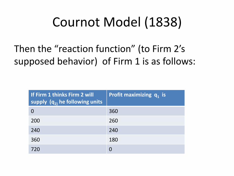
Then the “reaction function” (to Firm 2’s supposed behavior) of Firm 1 is as follows:

If Firm 1 thinks Firm 2 will supply (q2) he following units

Profit maximizing q1 is

0 360

200 260

240 240

360 180

720 0

Cournot Model (1838)

Cournot equilibrium is determined at the intersection of the reaction functions of the two players.

Cournot Model (1838)

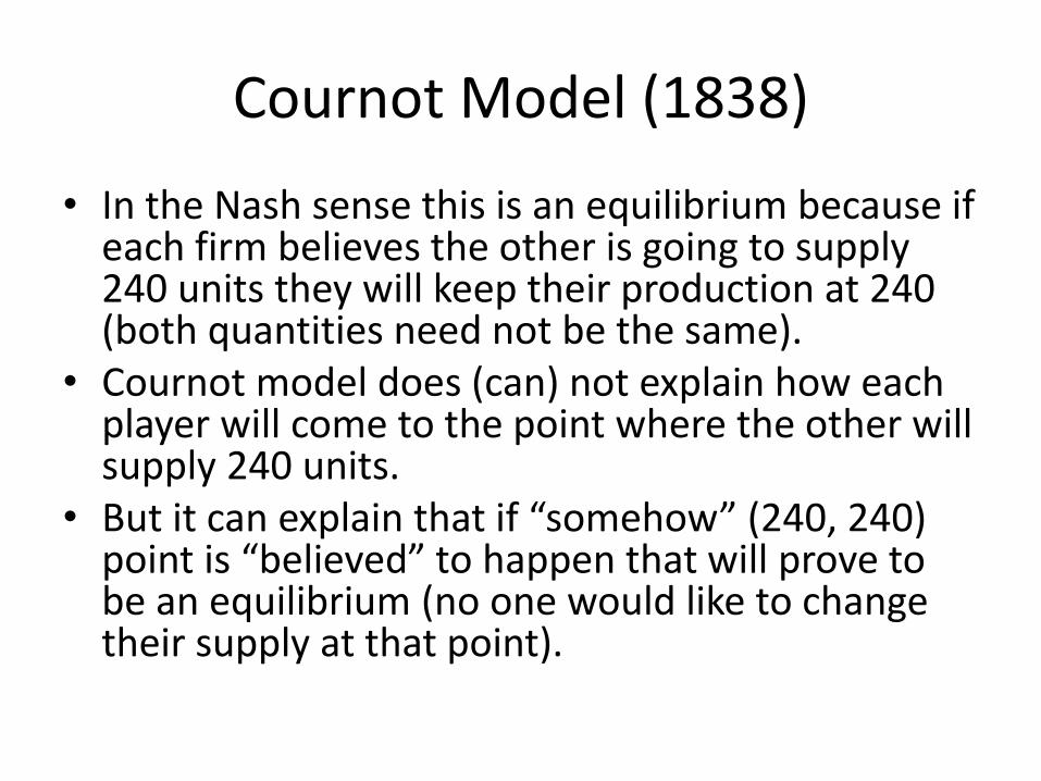
• In the Nash sense this is an equilibrium because if each firm believes the other is going to supply 240 units they will keep their production at 240 (both quantities need not be the same).

• Cournot model does (can) not explain how each player will come to the point where the other will supply 240 units.

• But it can explain that if “somehow” (240, 240) point is “believed” to happen that will prove to be an equilibrium (no one would like to change their supply at that point).

Cournot compared to Cartel and Competitive Equilibrium

Cournot vs Cartel

• When they do not cooperate (Cournot), the players will produce a total of 480 points sold at USD 0,52.

• If the two players cooperated (colluded), they would produce at the Monopoly level (360 units sold at USD 0,64).

• So from the point of view of the consumers, non-cooperating (competing) oligopolists are better than colluding ones. The consumer surplus is higher. Lerner index is lower for Cournot oligopolists: – Cournot (p-MC)/p=46% – Cartel (p-MC)/p=52%

– Note: MC is constant at USD 0.28

Cournot vs Competitive Equilibrium

How about the Cournot solution vs competitive solution?

• Competitive solution maximizes social welfare (consumer surplus + producer surplus). In that sense it represents the social optimum.

• Consumer surplus under CE is higher than Cournot solution but the firm profits are less. Overall, Cournot oligopolists cause a DWL to the society.

Bertrand Model

In the Cournot model, the firms set their quantities viewing the reaction of their rivals.

In the Bertrand model, they are supposed to behave a little differently; the firms set their prices.

The goods are homogenous. Thus firm assumes the rival’s price is fixed and tries to capture the market by reducing the price a little bit. Such thinking will lead to reduction of the price until

P=MC.

Bertrand Model

How does the residual demand curve for Firm 1 look like and why? Key to understand the chart is that a slight difference in price makes the market be served by only one of the firms. If the prices of both firms are the same, that we assume they equally share the narket.

Bertrand Model: best response functions

The Bertrand equilibrium is at p=MC. The best response function of Firm 2 lies slightly below the 45 degree line; it wants to charge a little lower than p1 to capture the market. Likewise, Firm 1’s best response function lies a little to the left of 45 degree line. The only intersection point is at MC. None of the two can charge lower than the MC.

von Stackelberg Model

In von the Stackelberg Model, players select output (as in the Cournot model) but the game is played in two stages. In the first stage the “leader” selects the output level q1. In the second stage “follower” reacts by selecting its best output q2 at corresponing to q1.

von Stackelberg Model

Firms have identical cost functions and there is perfect information. So the leader knows the response function of the follower.

In this example, best output for Firm 1 is 360 units. That makes the follower produce at 180 units.

von Stackelberg Model: Extensive Form Representations

Von Stackelberg games can also be analysed by using extensive forms.

von Stackelberg ve Cournot and Bertrand Models

Von Stackelberg solution is the closest to social optimum.

Comparing the predictions of the three models

n=1 n falls n increases

Cournot equilibrium

Monopoly Converges monopoly equilibrium

Converges competitive equilibrium

Bertrand equilibrium

Monopoly Compettitive equilibrium for n>=2 (assuming no capacity constraints)

Compettitive equilibrium for n>=2 (assuming no capacity constraints)

Von Stackelberg Monopoly Converges monopoly equilibrium

Converges competitive equilibrium

Introduction to multiperiod games

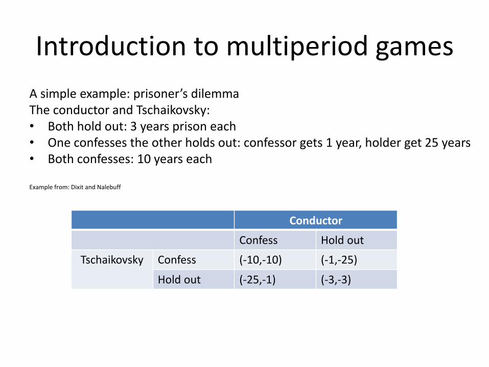
A simple example: prisoner’s dilemma The conductor and Tschaikovsky: • Both hold out: 3 years prison each • One confesses the other holds out: confessor gets 1 year, holder get 25 years • Both confesses: 10 years each Example from: Dixit and Nalebuff

Conductor

Confess Hold out

Tschaikovsky Confess (-10,-10) (-1,-25)

Hold out (-25,-1) (-3,-3)

Prisoner’s dilemma for Firms 1 and 2: single period case

q1 =240 is the dominant strategy for Firm 1.

q2 =240 is the dominant strategy for Firm 2.

Where do they end up in terms of profits?

Prisoner’s dilemma for Firms 1 and 2: single period case

You can fool some of the people all of the time, and all of the people some of the time, but you can not fool all of the people all of the time.

Abraham Lincoln

What happens if the game is to be played many times in the future?

Prisoner’s dilemma for Firms 1 and 2: single period case

In infitely played games, the players will have opportunity to “signal” its intentions and/or punish the other though illegal.

By doing that (cooperating) they can decrease output and increase profits. If the other party cooperates, their profits will both increase. If the other party does not cooperate, the Firm can punish the other by increasing output.

How does that affect the society?

Prisoner’s dilemma for Firms 1 and 2: multi -period case

q1 =240 is the dominant strategy for Firm 1.

q2 =240 is the dominant strategy for Firm 2.

Where do they end up in terms of profits?