Federal Reserve Bank of Dallas Globalization and Monetary Policy Institute

Working Paper No. 130 http://www.dallasfed.org/assets/documents/institute/wpapers/2012/0130.pdf

Market Structure and Exchange Rate Pass-Through*

Raphael A. Auer Raphael S. Schoenle Swiss National Bank Brandeis University

October 2012

Abstract In this paper, we examine the extent to which market structure and the way in which it affects pricing decisions of profit-maximizing firms can explain incomplete exchange rate pass-through. To this purpose, we evaluate how pass-through rates vary across trade partners and sectors depending on the mass and size distribution of firms affected by a particular exchange rate shock. In the first step of our analysis, we decompose bilateral exchange rate movements into broad US Dollar (USD) movements and trade-partner currency (TPC) movements. Using micro data on US import prices, we show that the pass-through rate following USD movements is up to four times as large as the pass-through rate following TPC movements and that the rate of pass-through following TPC movements is increasing in the trade partner's sector-specific market share. In the second step, we draw on the parsimonious model of oligopoly pricing featuring variable markups of Dornbusch (1987) and Atkeson and Burstein (2008) to show how the distribution of firms' market shares and origins within a sector affects the trade-partner specific pass-through rate. Third, we calibrate this model using our exchange rate decomposition and information on the origin of firms and their market shares. We find that the calibrated model can explain a substantial part of the variation in import price changes and pass-through rates across sectors, trade partners, and sector-trade partner pairs. JEL codes: E3, E31, F41

* Raphael Auer, Swiss National Bank, Börsenstr. 15, P.O. Box Ch-8022, Zürich, Switzerland. +41-631-38-84. raphael.auer@snb.ch. Raphael Schoenle, Mail Stop 021, Brandeis University, P.O. Box 9110, 415 South Street, Waltham, MA 02454. 1-617-680-0114. schoenle@brandeis.edu. This research was conducted with restricted access to the Bureau of Labor Statistics (BLS) data. We thank project coordinators Kristen Reed and Rozi Ulics for their substantial help and effort and Rawley Heimer and Miao Ouyang for excellent research assistance. We also thank Gita Gopinath, Anthony Landry, and Romain Ranciere, as well as participants at the Milton Friedman Institute Conference on Pricing at the University of Chicago, the University of Geneva, the University of Berne, the University of Munich, the Microeconomic Aspects of the Globalization of Inflation Conference at the Swiss National Bank, the 2011 Midwest Macro Meetings at Vanderbilt University, the 2011 European Economic Association Meetings at the University of Oslo, the 2012 meetings of the Austrian Economic Association at the Technical University of Vienna, the 2012 meetings of the Society for Economic Dynamics in Limmasol, the 2012 CEPR Summer Symposium in International Macroeconomics in Tarragona, the 2012 NBER Summer International Finance and Macroeconomics workshop and in particular an anonymous referee at the SNB Working Paper series for helpful comments and suggestions. The views in this paper are those of the authors and do not necessarily reflect the views of the Swiss National Bank, the Federal Reserve Bank of Dallas or the Federal Reserve System.

1 Introduction

Studying firms’ pricing-to-market decisions is one of the important research topics in international

macroeconomics because it relates to the movement of international relative prices, expenditure

switching and the adjustment of global imbalances, and imported inflation. Moreover, this line of

research can also inform us about the nature of price-setting, which features prominently in most

macro-economic models.

The recent empirical literature estimating exchange rate pass-through at the good level has

yielded important insights into firms’ pricing behavior following exchange rate shocks.1 While the

results have uncovered much heterogeneity along multiple dimensions of firm or good character-

istics,2 a common finding is that pass-through, even when estimated at the dock and over long

horizons, is quite incomplete: import prices do not move one-to-one with the exchange rate.

Incomplete long-run pass-through can be explained by markups being adjusted to accommodate

the local market environment, a channel first pointed out in Krugman (1986) and Dornbusch (1987)

and more recently in Melitz and Ottaviano (2008), Atkeson and Burstein (2008), Chen et al. (2009),

Gust et al. (2009, 2010), and Gopinath and Itskhoki (2011).

In this paper, we contribute to this literature by identifying how exchange rate shocks affect

the market environment differently in different sectors depending on the mass and size distribution

of firms that is affected by a particular exchange rate shock. Because we focus on the variation

in pass-through rates across both sectors and trade partners, we are able to discern the role of

market structure from alternative explanations, that is, from the view that costs simply do not

move one-to-one with the exchange rate.

Our analysis proceeds in three steps. In the first step of our analysis, we document several

salient facts showing that pass-through rates vary across trade partners and sectors depending on

mass of firms affected by a particular exchange rate shock.

1While some of these studies focus on structural analysis of exchange rate pass-through in single industries (seeKnetter (1989) and Knetter (1992) and the analysis of pricing-to-market practices in Verboven (1996), Goldbergand Verboven (2001, 2005) for the car industry, Hellerstein (2008) for the beer industry, and Nakamura and Zerom(2010) for the case of the coffee industry), our approach is more closely related to the reduced-form analysis ofpass-through rates in datasets spanning many industries (see Gopinath and Rigobon (2008), Gopinath and Itskhoki(2010), Gopinath et al. (2010), and Nakamura and Steinsson (2008a)). It is also related to the work of Fitzgeraldand Haller (2010), who use plant-level prices of identical goods sold on different markets to study pricing-to-marketdecisions.

2When evaluating prices at the dock (that is, net of distribution costs), the main dimensions along which theheterogeneity of pass-through rates are identified include the currency choice of invoicing as in Gopinath et al. (2010),Goldberg and Tille (2009), Bacchetta and van Wincoop (2005), inter- versus intra-firm trade as in Neiman (2010),multi-product exporters as in Chatterjee et al. (2011), sectoral import composition as in Campa and Goldberg (2005);Goldberg and Campa (2010), and input use intensity. When evaluating retail prices, the share of the distributioncosts may matter for pass-through as found by Bacchetta and van Wincoop (2003) and Burstein et al. (2003), whilethe movement of margins seems to play only a minor role as shown in Goldberg and Hellerstein (2012). Generally,also the size and origin of the exchange rate movement matter for pass-through (see Michael et al. (1997) and Bursteinet al. (2005, 2007)) as does the general equilibrium interaction between exchange rate volatility, invoicing currencychoice, and pass-through rate (see Devereux et al. (2004)).

2

To document these salient facts, we first show that exchange rate movements are passed through

into US import prices significantly differently when the bilateral exchange rate change is driven

specifically by the trade partner currency as opposed to when it is reflecting a broad movement

of the USD against all trade partners. To this purpose, we decompose bilateral exchange rate

movements into broad USD movements common to all importers and into trade-partner currency

(TPC) specific movements. We then estimate pass-through following these two different shocks

using micro data on US import prices. We find that pass-through at horizons up to two years is

equal to up to 31% following a USD movement, but only up to 8% following a TPC movement.

The next salient fact we document is that pass-through rates vary with the mass of firms that

is affected by the TPC exchange rate shock. For TPC movements, we find that the rate of pass-

through is increasing in the trade partner’s sector-specific import share.We find the importance of

sector-specific market share to be economically very large. Over longer horizons, the rate of pass-

through of a hypothetical US trade partner with an import share near zero equals around 10%,

while the pass-through rate is nearly four times as large for a hypothetical trade partner with a

market share of 100%. Nearly one third of the aggregate two-year pass-through rate in our sample,

equal to 16%, is explained by the fact that trade partner market shares are non-negligible.

We view these patterns in the data as a strong indicator that the rate of pass-through is highly

dependent on the way in which an exchange rate shock and a sector’s market structure interact

to shape firms’ equilibrium price responses to exchange rate movements. However, these reduced-

form estimations are limited in nature because they only capture a very coarse element of market

structure, namely the combined market share of firms affected by a specific exchange rate shock.

Heterogeneous firms of different size potentially react differently to the same exchange rate shock,

so that the entire size distribution of firms should matter for pass-through. Indeed, Berman et al.

(2012) find that pass-through varies substantially according to firm size.3 Thus, differences in the

distribution of firm sizes across sectors, trade partners, and trade partner-sector pairs are potentially

also important in explaining pass-through.

In the second step of our analysis, we therefore use the additional structure from a parsimonious

model of oligopoly pricing, following Dornbusch (1987) and Atkeson and Burstein (2008), to include

information on the entire size and origin distribution of firms into our estimation. We first document

how oligopoly-pricing in the preference setup of Dornbusch (1987) and Atkeson and Burstein (2008)

determines pass-through rates, identifying two elements how a sector’s market structure affects the

pass-through rate. The first element is that the rate at which a firm reacts to changes in the

exchange rate depends on its market share. The average direct price response of the set of firms

affected by a given exchange rate shock thus depends on the distribution of their market shares. The

3Relatedly, Manova and Zhang (2012) show that export pricing patterns are related to firm characteristics, whileFeenstra (1994), Andrade et al. (2012) and Garetto (2012) document how pricing-to-market decisions are affectedby firm market share. Auer et al. (2012), who as Garetto (2012) use the dataset of car prices sold on five Europeanmarkets Goldberg and Verboven (2001, 2005), document how the quality of the produced good affects pricing-to-market and exchange rate pass through.

3

second element is that the price changes of firms from a trade partner affect the industry’s general

price level and thus the pricing decisions of all firms in the industry. The first-round impact on the

general price level is proportional to the combined market share of firms from the trade partner.

Moreover, there is a further amplification of the price shock since all other firms in the industry

react to the changing general price level, multiplying the initial impact. In this sense, pass-through

is affected by the sector’s entire market structure also if only few firms are affected by a given

exchange rate movement.

In the third step of this analysis, we map the developed theoretical pricing framework back

to the BLS micro data. We then test it in two ways: first, we test whether this preference setup

can match actual price changes and second, if it can explain the heterogeneity of pass-through

rates across trade partners when it is calibrated using the TPC movements on the one hand and

information on a sector’s market structure one the other hand.

We find strong evidence for the predictions of the model relating market structure and pass-

through when we estimate it using the TPC movements and information on the market structure

of the entire sector.4 The model is able to explain both qualitatively and quantitatively the size

of price changes, as well as a substantial part of the variation in pass-through across sectors and

trade partners.

We undertake two sets of exercises. In the first set, we show that the model can explain actual

price changes in the BLS micro data when we relate model-predicted to actually observed price

changes at the firm level. For this set of tests, we construct predictions of firm-specific price

changes using the theoretical pass-through predictions and our exchange rate decomposition. We

then relate the predicted to the actually observed price changes, which serves mostly to establish

how simulation assumptions, sample restrictions, and addition of relevant fixed effects impact our

results.

We document the explanatory power of the TPC price change predictions under alternative

assumptions and then document the explanatory power of our predictions following both TPC and

USD movements. In a further robustness analysis, we examine the details of mapping our theory to

the BLS data, show the variation in the data that is behind our results by including various fixed

effects, and exclude subgroups of countries. For this set of exercises, we document both the average

response of actual to predicted prices and also, the relation between these actual and, following

Gopinath and Rigobon (2008) to address nominal price rigidities, predicted prices conditional on a

non-zero price change.

These empirical exercises provide strong evidence for the predictive power of the Dornbusch-

Atkeson-Burstein setup in explaining firms’ pricing responses to exchange rate movements: not only

4This exercise is related to Pennings (2012), who undertakes a similar calibration to evaluate the cross-currencyrate of pass-through, that is, the effect of the USD/Euro exchange rate on the prices that Japanese firms charge inthe US. Gopinath and Itskhoki (2011) directly estimate the importance of such complementarities using the averagechange of competitor’s prices. Bergin and Feenstra (2009) also study such cross-currency price effects.

4

do predicted price changes correlate significantly with actual price changes both conditionally and

unconditionally, but the coefficients of the conditional estimates are closer to 1 and in not few cases

statistically indiscernible from 1, that is, our point estimates are also quantitatively good predictors

of actual price changes. Overall, in terms of R2, we can explain up to 19% of the non-zero price

changes in the differentiated goods subsample with the USD and TPC induced price changes. We

also show that our setup matches the overall distribution of price changes better than a benchmark

constant-markup model.

In the second set of the emprical exercises, we aggregate our predictions up to the industry-

country level and show that our theory is economically highly significant in explaining pricing

behavior at these important aggregate levels.5 Our predicted price changes correlate with actual

ones at very high levels of significance and they often do so at a rate that is statistically not differ-

ent from 1, that is we do not only qualitatively explain pass-through rates, but also quantitatively.

When evaluating differences in pass-through rates, we document that a substantial part of the vari-

ation in pass-through across sectors and trade partners – approximately a third – can be explained

by differences in the mass and size distribution of firms across the trade partners.

Overall, we draw three conclusions from our theoretical and empirical analysis: First, we con-

clude that the effect of the exchange rate on the competitive environment and, in turn, on equilib-

rium markups is substantial. This highlights the importance of including price complementarities

in macroeconomic models, may these complementarities arise from strategic motives as in Kimball

(1995) and Dotsey and King (2005) or from the shape of the utility function as in Gust et al. (2010)

and Chen et al. (2009). This conclusion has also important modeling implications for firms’ pricing

decisions in the domestic economy: if the optimal price of a firm reacts strongly to a cost shock,

already small menu costs can substantially reduce the frequency of price changes (see, for exam-

ple, Bils and Klenow (2004) and Nakamura and Steinsson (2008b) for evidence on how frequently

domestic firms change prices).

Second, we conclude that the Dornbusch-Atkeson-Burstein style departure from the case of

constantly elastic demand greatly improves our understanding of pass-through rates in the data.

As Atkeson and Burstein (2008), we do not view the proposed model as a general model of pricing-

to-market, but rather as the simplest possible departure from the case of constant elasticity demand.

Demonstrating how far the calibrated model is from the data can inform us whether more complex

theories of pricing to market are necessary to reconcile theory and data. From an empiricist’s point

of view, our results suggest that knowing the distribution of firm’s market shares is sufficient to

calculate aggregate pass-through rates.

Third, from a policy maker’s perspective, our findings are relevant given the economic magnitude

5In this set of exercises, the sample is much smaller than in the first set, as we need a large number of observationsto estimate one pass-through rate. However, the second set focuses on the economic significance: we can analyzehow much of the empirically observed variation in pass-through rates across sectors, trade partners and sector-tradepartners can be explained with differences in market structure.

5

of the uncovered relations. The finding that pass-through following broad USD movements is very

large gives rise to a much bigger role for the exchange rate on inflation dynamics – especially

in times of large, permanent exchange rate evaluations – than is commonly assumed: the pass-

through response by individual firms is exactly then the largest when all exchange rates move in

the same direction vis-a-vis the dollar.6 Additionally, our findings reveal that the aggregate rate of

pass-through is large when the trade partner is either large or concentrated in specific sectors.

The structure of this paper is the following. We describe our exchange rate decomposition and

the resulting reduced-form pass-through estimations in Section 2. Section 2.3 examines whether

pass-through depends on trade partner market shares and the trade openness of U.S. sectors.

Section 3 presents the model, highlighting the role of firm- and trade partner- market shares for

pass-through, and Section 4 examines whether a calibrated version of the model can explain import

price adjustments and pass-through rates. Section 5 documents to what extent the model can

explain differences in aggregate pass-through rates. Section 6 concludes.

2 How are General and Trade-Partner Specific Exchange Rate

Movements Passed Through Into US Import Prices?

In this section, we discuss how we decompose changes in the nominal bilateral exchange rate into

broad USD movements on the one hand and trade-partner specific movements on the other hand.

Then, we show that pass-through is systematically different when the USD moves against all of its

trade partners rather than when the change in the bilateral nominal exchange rate is caused by

a trade partner movement against the rest of the world. A description of the data we use can be

found in Appendix B.

This exercise is motivated by theoretical considerations relating pass-through to how the market

environment changes with the exchange rate. For example, if we think along the lines of Atkeson

and Burstein (2008), where market power determines pass-through, pass-through should be very

different if all foreign firms face the same cost shock as opposed to when only a small set of firms

from a country such as Switzerland faces a cost shock. Theoretical models that highlight non-

strategic price complementarities such as Chen et al. (2009) or Gust et al. (2009) also predict that

pass-through should be higher when the USD appreciates against all countries since all exporters

experience the same cost shock in that case.

2.1 USD and Trade-Partner Currency Movements

Building on Glick and Rogoff (1995) and Gopinath and Itskhoki (2011), we decompose the bilateral

exchange rate into idiosyncratic TPC movements and broad USD movements. First, we define

6Such large import price movements, in turn, might also affect the prices domestic firms charge (a channel analyzedin Auer (2012)).

6

the USD/ROW exchange rate change for a specific trade partner as the import-weighted average

change of the log bilateral USD exchange rate against all countries except for the trade partner

under consideration. That is, if TP indexes the trade partner, the change of the USD exchange

rate against the rest of the world (ROW) except TP equals

∆USDROW−TP,t ≡∑

cε(C⊃{TP,USA})

ωc,t∆ec,t, (1)

where ∆ec,t is the bilateral exchange rate between the US country c and country c’s weight equals

its shares of US imports excluding country TP. To make sure that the weights are not contempo-

raneously related to current exchange rate movements, we take last year’s import share as current

weights:

ωTP,t ≡IMUS

TP,t−1∑c 6=TP,USA IM

USc,t−1

.

It is important to note that the USD/ROW exchange rate change differs for each trade partner due

to the inclusion of a different set of countries. Therefore, it differs from a standard trade-weighted

exchange rate. We discuss this difference further below.

Second, we define the “TPC exchange rate movement against the ROW” (TPC) as the difference

between the bilateral exchange rate change and the broad USD exchange rate change

∆TPCTP,t ≡ ∆ec,t −∆USDROW−TP,t. (2)

We note that ∆TPCTP,t is equal to the negative of the average change (using US weights) of the

trade partner currency against all countries other than the USA.7 This exchange rate decomposition

is similar in spirit to constructing an import-weighted exchange rate index and then interpreting

the residual difference of the bilateral nominal exchange rate and the import-weighted exchange

rate index as an idiosyncratic trade partner currency movement.

However, our approach is different in that takes into account the effect of large trade partners on

the import-weighted exchange rate index. For example, if the currency of a trade partner providing

15% of US imports appreciates by 10% against the USD, while all other exchange rates remain flat

7This can be verified by noting that for any three currencies USD, TPC, and c, the absence of arbitrage possibilitiesimplies that

∆USDTP,t = ∆USDc,t −∆TPCc,t

for any country c. Since the weights ωc,t sum to one, it is thus true that

∆USDTP,t =∑

cε(C⊃{TP,USA})

ωc,t (∆USDc,t −∆TPCc,t) .

Noting the definition of ∆USDROW−TP,t and ∆TPCTP,t then implies

∆TPCTP,t = −∑

cε(C⊃{TP,USA})

ωc,t∆TPCc,t.

7

against the USD, our decomposition will correctly measure a TPC movement of 10%. In contrast,

an approach based on the import-weighted exchange rate index would yield a TPC movement of

8.5% since the import-weighted exchange rate index itself moves by 10% ∗ 15% = 1.5%.

Using an import-weighted exchange rate index instead of our USD measure would make it diffi-

cult to econometrically disentangle pass-through following USD movements as opposed to following

TPC movements. Even worse, not controlling for the effect of large trade partners on the import-

weighted exchange rate index would introduce a mechanical bias in the regressions estimated in

Section 2.3 below that relates import shares to the rate of TPC pass-through, as large trade part-

ners would by construction have a lower TPC volatility. Because both US imports and the BLS

import price data are dominated by large trade partners such as China, Canada, and Mexico (over-

all import share in 2010: 19.2%, 14.5%, and 12.1% respectively), this problem is not trivial in the

data.8

Our decomposition is closely related to Gopinath and Itskhoki (2011), who use the residuals from

a regression of the trade-weighted exchange rate on the bilateral USD exchange rate as a measure of

broad USD movements; that is, they use the element of the US trade-weighted exchange rate that

is orthogonal to the bilateral one. While these two approaches of defining a broad USD movement

are numerically not too different, we find it conceptually easier to work with the deterministic

decomposition.9

More importantly, the main conceptual difference between Gopinath and Itskhoki (2011) and

our approach is due to our focus on TPC movements: we are interested in the pass-through rate

following the part of the bilateral exchange rate that is not driven by a general appreciation, that

is, our TPC movements are equal to the bilateral minus the ROW exchange rate. Gopinath and

Itskhoki (2011), in contrast, use the bilateral exchange rate directly and control for the ROW

exchange rate. While this difference is trivial for the analysis evaluating only the aggregate pass-

through rate (since the pass-through coefficients are linear transformations of each other), it matters

in sections 2.3 and 4, in which we interact TPC movements with each trade partner’s market share

and other sector-specific information.

8For the US, it is also common to estimate the pass-through rate of changes in the “Broad Exchange Rate” whichis an rate index constructed by the Federal Reserve Board giving a 50% weight on import share, 25% on export share,and 25% on a measure of “third-market competitiveness” as described in Loretan (2005). While the broad exchangerate index may be a useful concept when evaluating the effect of the exchange rate on the current account or themacro economy in general, we consider using only import weights a more relevant statistic when estimating how theaverage exchange rate and average import prices comove.

9The exact difference between these two approaches is that we only net out each country’s mechanical contributionto the trade-weighted exchange rate, whereas Gopinath and Itskhoki (2011) also include the covariance of the TPexchange rate with other exchange rates. For example, Iceland’s import share is minuscule (around 0.0002), so thatfor the Icelandic kronor, the change in the ROW exchange rate we construct is nearly identical to the change inthe US-trade-weighted exchange rate. However, since the kronor co-moves with other exchange rates, its regressioncoefficient on the US trade-weighted exchange rate is equal to 0.169. We note that despite of what this examplesuggests, the difference between our approach and the one in Gopinath and Itskhoki (2011) is not too sizeable. Thecorrelation between these two variables is equal to 0.79 and a regression yields a slope of 1.023 (which is significantlydifferent from 1).

8

2.2 Pass-Through Following TPC and USD Movements

We measure pass-through by estimating a stacked regression where we regress monthly import price

changes on monthly lags of the respective measure of the exchange rate. Following Gopinath and

Rigobon (2008), our baseline specification is

∆pi,c,t = αc +n∑j=1

βj∆ec,t−j+1 +n∑j=1

γTPj ∆πTPc,t−j+1 + εi,c,t, (3)

where i indexes goods, c trade partners, αc is a country fixed effect, n measures the length of the

estimated pass-through horizon and varies from 1 to 25, and ∆ec,t−j is the change in either the

log of the nominal, USD, or TPC exchange rate. ∆πTPc,t is the monthly inflation rate in the foreign

country using the consumer price index. To obtain the n-months pass-through rate, we sum the

coefficients up to the respective horizon. Alternatively, we also estimate a joint specification:

∆pi,c,t = αc +n∑j=1

βUSDj ∆USDROW−c,t−j+1 +n∑j=1

βTPCj ∆TPCc,t−j+1 +n∑j=1

γj∆πTPc,t−j+1 + εi,c,t (4)

where ∆TPCc,t corresponds to the TPC movement of country c and ∆USDROW−c,t to the USD

movements of the exchange rate for country c.

Figures 1 and 2 and Table C.1 in Appendix C present our results from estimating Equations (3)

and (4). Column (1) in Table C.1 presents these estimates for the nominal bilateral USD exchange

rate. The rows list the cumulative pass-through coefficient equal to∑n

j=1 βj for 1, 3, 6, 12, 18,

and 24 month(s) and the corresponding standard error. All summed coefficients are significant at

the 1% level. Columns (2) and (3) then repeat this specification using the USD-movement and the

TPC movement respectively.

When we estimate pass-through for each component of the exchange rate, we find that USD

movements are passed through at more than twice the rate of nominal movements. For example,

at the six-month horizon, USD pass-through is estimated at 31%, while nominal exchange-rate

pass-through is estimated at only 11% (see third row and columns (1) and (2), respectively). At

the two-year horizon, USD pass-through is at 32% while the rate of pass-through conventionally

estimated is at 15%. The result of high USD pass-through rate confirms the finding of higher trade

weighted exchange rate pass-through of Gopinath and Itskhoki (2011) and also agree with them

quantitatively.10

The striking novel result of our analysis comes from the estimation of TPC currency pass-

through: for any horizon, TPC exchange rate pass-through is even lower than bilateral exchange

10Any residual differences between and our results and Gopinath and Itskhoki (2011) can be attributed to differencesin the steps in data construction of the micro data and our exchange rate measures, which are derived as weightedsums and deviations thereof. Also, our sample selects out any time series with less than 72 months of data and dropsBLS country codes below 1000 which are aggregates of more than one country.

9

rate pass-through which is already less than USD pass-through. At the two-year horizon, TPC is

only 7.34% compared to 32% USD pass-through as columns (2) and (3) show.11

Figure 1 summarizes this finding graphically, based on the separate pass-through estimations

of columns (1) to (3) in Table C.1 for all lagged horizons. It shows the pass-through estimates that

can be attributed to a movement of the USD against all partner currencies, a movement of the

trade partner currency against the rest of the world or simply a nominal exchange rate movement.

While USD pass-through is larger at all monthly horizons, it is at approximately 35% at horizons

over one year. Trade-partner pass-through at that horizon is estimated at around only 5%, while

nominal exchange rate pass-through is estimated at around 10%.

When we jointly estimate pass-through of our two components of the nominal exchange rate,

that is, broad USD and TPC movements, we find an even stronger impact of broad USD movements

on U.S. import prices. Figure 2 as well as Columns (4) and (5) in Table C.1 present the same

comparison for the joint pass-through rates following USD and TPC movements, which is estimated

using Equation (4). In this joint estimation, the USD pass-through rate is also estimated to be

between three to over four times as large as the TPC pass-through rate. The TPC pass-through is

low, topping out at 10.15% at the one-and-a-half years horizon. In this joint estimation, we can test

whether USD pass-through is the same as TPC pass-through in a statistical sense, or not. They

are so at the 1% significance level at all horizons except the 24 months one. This is also graphically

demonstrated in Figure 2 using confidence bands.

In Appendix C, we document that the difference in pass-through rates following TPC and USD

movements is not driven by specific sectors or specific countries. We present robustness checks

that confirm that pass-through of broad USD movements is larger than trade-partner or bilateral

exchange rate pass-through also at the country and two-digit NAICS level, that is, broad USD

movements are passed through into U.S. import prices at a substantially higher rate than trade-

partner movements.

Despite these results, a further important concern is that when estimating Equation (3), we

are not properly controlling for changes in firms’ production costs. A USD movement could be

associated with a very high cost shock as it moves the world market prices for intermediate goods.

Also a TPC shocks could simply reflect productivity growth in the trade partner, which would also

influence the prices of importers for reasons other than the exchange rate fluctuation.12

11It is unlikely that the different PT rate following TPC and USD shocks is explained by differences in the propertiesof these exchange rate series. During 1994-2004 and in the group of OECD economies, the standard deviation ofmonthly exchange rate changes is 3% for the bilateral exchange rate, 1.3% for the USD movements, and 2.6% for theTPC movements. Persistence of these three time series is very similar: in this sample, the sum of AR coefficients upto 12-month lagged levels of the exchange rate is equal to 0.803, 0.794, and 0.814 for the bilateral, USD movements,and TPC movements respectively.

12In a discussion of our paper, Landry (2011) re-estimates specification (3) using our exchange rate decompositionon the dataset of Baxter and Landry (2010). The latter dataset includes the prices of identical IKEA goods sold ondifferent markets, with the advantage that one can control for changes in the cost of a good sold on other markets,yielding a much better cost control than in our specification. He finds a 2-year rate USD pass-through nearly identicalto our specification. See also Baxter and Landry (2010).

10

To address this concern, we proceed to utilizing the cross section of our dataset, that is variation

in the import share of a specific country across the sectors. While the exchange rate is endogenous

to average productivity growth, this gives us additional sectoral variation in the extent to which

prices react to the exchange rate. We thus proceed to examine how the sectoral import share

correlates with the TPC pass-through rate.

2.3 Market Share and Pass-Through

In this subsection, we show that TPC pass-through is increasing in the import share of the country

from which the firm is exporting. This suggests that low TPC pass-through may be due to individual

trade-partner on average having low market shares.

We show that the response to TPC movements is dependent on the market share of the respective

importers. We define the sector-specific import share of trade partner c in sector k as

mc,k =Importsc,k

World Importsk

Then, we run an augmented, reduced-form pass-through specification where we interact the sector-

specific import share of the trade partner with TPC exchange rate movements:

∆pi,c,k,t = αc +

n∑j=1

βj∆TPCc,t−j+1 +

n∑j=1

γjmc,k∆TPCc,t−j+1 +mc,k + εi,c,k,t, (5)

where i denotes a good, αc is a country fixed effect, k a sector, n varies from 1 to 25, and ∆TPCc,t is

the change in the trade-partner currency, and mc,k denotes the sector-specific import share measure

of country c in a given six-digit NAICS sector k for the year 2002.

To obtain the n-months direct rate of pass-through, we sum the coefficients βj up to the respec-

tive horizon. To obtain the indirect effect working through the measure of market power, we sum

the coefficients γj up to the respective horizon. When we multiply the sum of γj with the average

respective market share from the data, this yields the effective interaction with the right economic

magnitude.

The three lines displayed in Figure 3 reflect the pass through rate following a TPC shock for

three sectors in which firms from the trade partners make up around 0% (that is, there are some

importers from the TP so that prices exist, but they are negligible in size; see solid line), 31%

(which is equal to the median of mc,k in our data; see dotted line) and 100% (solid marked line).

For each lag length n, the solid line corresponds to the sum of the coefficients∑n

j=1 βj in Equation

(2.3). The difference between the solid marked line and the solid line corresponds to the sum of

the interaction coefficients∑n

j=1 γj in Equation (2.3).

We find that there is a sizeable impact of market share on the degree of exchange rate pass-

through. In a sector in which a trade partner has around 0% of the import market, the TPC

11

pass-through rate is around 13% at the 2 year horizon. In a sector where the trade partner supplies

nearly 100% of imports, the TPC pass-through rate is equal to 38% at the same horizon, that is,

it is 25 percentage points higher (0.25 is equal to the interaction term∑24

j=1 γj in the estimation of

Equation (2.3)).

For a sector with median import share (the median of mc,k is equal to 31%), the average long-

run pass-through rate is equal to 21%, of which 0.31 ∗ 0.25 = 0.0775 is attributed to the interaction

term, that is, to the fact that the median sector has a nonnegligible import share. Thus, in economic

terms, non-zero import shares explain more than a third of the long-run TPC pass-through rate

for the typical firm.

We note that the above-described salient facts relate the total importer’s market share to

pass-through rate, but are mute about the relationship between firm-specific market share and

pass-through. In fact, Berman et al. (2012) document that large firms change their prices less to

an exchange rate movement than do small firms. The difference between Berman et al. (2012)’s

findings and ours is that we here consider a country’s market share, while Berman et al. (2012)

consider firm-specific market shares. We connect these two insights in the next section.13

3 Market Structure and Pass-Through: Theory

In the preceding analysis, we have documented that there is a strong reduced-form relationship be-

tween the degree of pass-through and the combined market share of the firms that are affected by

the exchange rate movement. We have suggested that the documented stylized facts are consistent

with pricing theories that argue for the importance of pricing-to-market and price complementari-

ties.

We next develop a simple model of pricing-to-market in this spirit that is based on Dorn-

busch (1987) and, in its log-linearized version on Atkeson and Burstein (2008) to formalize these

statements and to guide our main empirical analysis. In particular, the aim of this section is to

develop a framework that conceptualizes “market structure” in the context pricing-to-market deci-

sions. While there are four commonly recognized types of market structures – perfect competition,

monopolistic competition, oligopoly, and monopoly– a realistic mapping of market structure into

pass-through rates requires a more gradual definition. We thus use the framework of Dornbusch

(1987) and Atkeson and Burstein (2008) to guide our theoretical analysis and show how the pass-

through rate depends on the number of firms that is affected by an exchange rate movement, their

respective market shares, and the firm size distribution in the entire industry.

We note that many previous studies have used these preferences to analyze pricing-to-market

13The finding that the total market share of all firms originating from a specific trade partner is related to Feenstraet al. (1996), who develop a differentiated products model in which firms compete a la Bertrand to show that therelationship between the pass-through rate and the trade partner market share is non-linear. They find evidencefor the theoretically predicted non-linearity when they examine the relationship between exporter market share andpass-through in the global car industry.

12

decisions as, for example, Yang (1997). Given that it is well known from previous work that markups

are variable and optimal prices respond to the prices of competitors under such preferences, we

view our contribution as adapting this well-established theory to a microeconomic dataset and

highlighting how market structure affects the degree of exchange rate pass-through. We first show

that the reduced-form relationships that we have estimated above can indeed be rationalized as the

outcome of this preference setup. Then, we explicitly discuss how other aspects of market structure

influences pass-through rates.

We also note that, as Atkeson and Burstein (2008), we do not view the proposed model as a

general model of pricing to market, but rather as the simplest possible departure from the case

of constant elasticity demand. Demonstrating how far the calibrated model is from the data can

inform us whether more complex theories of pricing to market are necessary to reconcile theory

and data.

3.1 The Dornbusch-Atkeson-Burstein Model

Our model relies on the preferences introduced by Dornbusch (1987) in which markups are vari-

able since a firm’s market share affects the firm’s elasticity of substitution. This preference setup

captures two main economic forces: first, pass-through is less than one as markups adjust to a cost

shock and second, not only a firm’s own costs matter, but also the prices of all other firms.

The preferences are given by a two-tiered “love of variety” utility/production function setup in

which consumers consume the output of sectors k and the output of each sector is produced by

combining varieties n within each sector.

On the production side, within each sector there exist a number Nk of individual firms each

holding the monopoly to produce an input variety. All input varieties within a sector are then

used as inputs by competitive firms combining these inputs into the sector composite yk using a

production function that features a constant elasticity of substitution. On the preference side, as

in Dixit and Stiglitz (1977), consumers have preferences with constant-elasticity demand for each

sector’s total output.

Final consumption c is produced by competitive firms aggregating input goods into

c =

(∫ 1

0y

(η−1)/ηk dk

)η/(η−1)

Each final producer’s optimization yields

yk =

(PkP

)−ηc, (6)

where P is the unit price of the final output and equal to(∫ 1

0 P(1−η)k dk

)1/(1−η). In each sector k,

13

each input is produced by a set of n ∈ N monopolists, but the sector itself is competitive and

produces using only the inputs with a production function given by

yk =

(N∑n=1

q(ρk−1)/ρkn,k

)ρk/(ρk−1)

We allow for the fact that ρk, the elasticity of substitution between varieties may be sector-specific.

Cost minimization yields the price of the sector-composite as Pi,k =(∑N

n=1 p(1−ρk)n,k

)1/(1−ρk)and

demand for each individual input yn,k as

qn,k = yk

(Pn,kPk

)−ρk(7)

A key assumption of this preference framework is that

ρk > η ≥ 1,

that is, if we think of two sectors “Trousers” and “Shoes” and two shoe varieties “Reebok” and

“Nike,” we assume that it is easier to substitute away from Reebok to Nike than it is to substitute

from shoes to trousers. We also assume that ρk > 1 so that markups are finite.

Price Setting by Variety Monopolists. Dornbusch’s main departure from Dixit and Stiglitz

(1977) is that firms are non-negligible in size within a sector, so that each firm has an impact on

the aggregate price index of the sector, which it takes into account when setting its price.

Each variety producer faces a constant marginal cost ωn, which may include iceberg transporta-

tion costs and maximizes profits subject to demand derived from (7) and (6).

Given the two-tiered utility/production setup and the fact that the production elasticity ρk

differs from the demand elasticity over sector composites η, the first order condition of a firm with

a non-negligible market share in sector k implies a pricing rule of that is dependent on the firm’s

market share sn,k:

p∗n,k =ε (sn,k)

ε (sn,k)− ε (sn,k)ωn,k (8)

ε (s) =

[1

ρk(1− sn,k) +

1

ηsn,k

]−1

Since ρ > η, a firm’s perceived demand elasticity is decreasing in its market share. Consequently,

the equilibrium markup is increasing in the firm’s market share.

This preference framework cannot easily be solved for analytically. Atkeson and Burstein (2008)

show, however, that a loglinearization around the steady state results in a straightforward calibra-

14

tion of how cost changes translate into prices changes. This log-linearization yields

Pn,k = Γ (sn,k) sn,k + wn,k (9)

sn,k = (ρk − 1)(Pk − Pn,k

)where a denotes a deviation in logs from the steady state and where Γ (sn,k) measures the

responsiveness of the markup to the market share and is equal to Γ (sn,k) =sn,k(1/η−1/ρk)

1−(1−sn,k)/ρk−sn,k/η> 0.

We note that Γ (sn,k = 0) = 0 and that Γ (sn,k = 1) = 1/η−1/ρk1−1/η > 0. Pk is the percentage change

in the price index of sector k and is equal to Pk =∑

jεNksj,kPj,k.

14

3.2 Market Structure and Pass Through

With the log-linearized recursive pricing formula (9), it is straightforward to show how market

structure affects the rate of pass-through. Since

Pn,k = Γ (sn,k) (ρk − 1)(Pk − Pn,k

)+ wn,k,

collecting Pn,k terms yields a recursive pricing formula that relates each price change to a linear

combination of all other price changes and the firm’s cost change:

Pn,k = γn,kPk + αn,kwn,k (10)

Here, γn,k =Γ(sn,k)(ρk−1)

1+Γ(sn,k)(ρk−1)is the rate at which firm n responds to changes in the general price

level for given own costs and αn,k = 11+Γ(sn,k)(ρk−1)

is the rate at which this firm reacts to its own

cost for a given general price level.

Proposition 1 The Equilibrium Price Change of firm n in sector k is equal to

Pn,k = γn,k︸︷︷︸n′s response to Pk

∑jεNk

sjαj,kwj,k

1−∑

jεNksjγj,k︸ ︷︷ ︸

Equilibrium Effect on Pk

+ αn,kwn,k︸ ︷︷ ︸n′s direct response to wn,k

(11)

Proof. In Appendix A.

In mathematical terms, there are two elements determining the rate of pass-through. The first

element leading to pass-through is the fact that firms directly change their price in response to

14As Atkeson and Burstein (2008), our approach abstracts from nominal price stickiness. Benigno and Faia (2010),who also use a variant of the Dornbusch (1987) preference setup and assume that firms are identical examine howtrade integration affects the degree of exchange rate pass through in the presence of price stickiness. In their setup,an increase of globalization is modeled as an increase in the share of foreign firms that are active in the domesticeconomy; they document that such globalization unambigously increases the rate of pass through also when menucosts are present.

15

marginal cost changes. The price change resulting from this is equal to the change in the firm’s

marginal cost wn,k multiplied by the firm’s sensitivity to its marginal costs αn,k.

The second element is the effect of the exchange rate on the general price level, which is affected

by market structure via three channels. The first channel is that if the exchange rate of a trade

partner moves, any firm j originating from this trade partner moves prices by αj,kwj,k. Denoting

the set of firms in sector k that originates from the trade partner by Nk,TP , the total impact on

Pk is thus equal to∑

jεNk,TPsjαj,kwj,k. The first channel thus depends on the total impact of

TP-firms on the general price level. The second channel through which market structure affects

pass-through works through second-round amplification because all firms in the industry react to

the change in the general price level, thus multiplying the initial impact by(

1−∑

jεNksjγj,k

)−1.

The third channel is that the firm n, in turn, reacts to changes in the general price level with a

rate of γn,k, which depends on its market share.

In economic terms, two elements of market structure are important for the rate of pass through:

on the one hand, the market share of each individual firm affects its responsiveness to its costs and

to the general price level. On the other hand, the combined market share of all firms from the

trade partner determines the mass of firms that are affected by the exchange rate shock and the

corresponding effect on the general price level.

In order to highlight these two effects separately, we next proceed with a simplification of the

equilibrium pricing Equation (11), in which only the second channel matters: we assume that

domestic firms and also firms from all trade partners are of equal size, so that only the number of

firms originating from a certain country matters for pass-through.

The price response to TPC and USD movements. We next document how price react to

TPC and USD shocks. For this, we assume that each firm’s cost is linearly affected by the exchange

rate ∆ec,t and we also allow for the presence of further idiosyncratic cost shocks εn,k

wn,k = ∆ec,t + εn,k.

recalling our definition of TPC and USD cost shocks (∆ec,t = ∆USDROW−c,t + ∆TPCc,t) implies

that

Pn,k =

(γn,k

∑jεNc,k

sjαj,k

1−∑

jεNksjγj,k

+ αn,k

)∆TPCc,t+

(γn,k

∑jεNk

sjαj,k

1−∑

jεNksjγj,k

+ αn,k

)∆USDROW−c,t+εn,k

(12)

where

εn,k ≡ γn,k

∑jεNk

sjαj,kεj,k

1−∑

jεNksjγj,k

+ αn,kεn,k.

We note that the difference in the response to TPC movements and to USD movements arises

because the set of firms affected by the exchange rate movement is different: For a TPC movement,

16

only firms from trade partner c face the exchange rate shock (thus the summation over jεNc,k).

For a USD movement, all importers are affected (thus the summation over jεNk). To highlight this

intution, we next analyze the case of equal sized firms.

Assuming Equal-Sized Firms. We first present intuition for our model by solving out the

case for equal-sized firms. This allows us to explain how the model generates predictions for both

price changes, pass-through and market structure. The predictions also align exactly with the cases

of our reduced-form estimations.

Proposition 2 Assume that all firms are of equal size so that the total number of firms equals

Nk, sn,k = 1/Nk, γn,k = γ, αn,k = α, and Γ (sn,k) = Γ/ (1− ρ) are equal for domestic and foreign

firms. Denote the fraction of firms from the US, a TP, and the ROW by nUS, nTP , and nROW

with nUS + nTP + nROW = 1, and corresponding price changes by PUS, PTP , and PROW . Since all

prices are denominated in US Dollars and we only analyze cost shocks originating from exchange

rate movements, normalize wUS = 0.

Then, one can show that

PTPC,c = γ1

1− γnTPα∆TPCc,t︸ ︷︷ ︸

Effect of TPC on Pk

+ α∆TPCc,t︸ ︷︷ ︸DirectCost Effect

+ εn,k. (13)

and

PUSD,c = γ1

1− γ(nROW + nTP )α∆USDROW−c,t︸ ︷︷ ︸

Effect of USD on Pk

+ α∆USDROW−c,t︸ ︷︷ ︸DirectCost Effect

+ εn,k. (14)

and it follows that

1. As long as the rest of the world is non-negligible, that is if nROW > 0, pass-through following

a USD movement is larger than following a TPC movement of the same size:

(γ(nROW + nTP ) + 1− γ) > (γnTP + 1− γ)

2. Pass-through following a TPC movement is increasing in TP market share:

∂ α1−γ (γnTP+1−γ)

∂nTP> 0

Proof. In Appendix A.

Allowing for Firm Heterogeneity. Not only the mass of firms, but also the entire distribu-

tion of firm size matters for pass-through. For example, for constant total exports, pass-through is

larger in a sector with very small firms than in one with at least one large firm. With the precise

17

definition of price changes developed in (11) above, the TPC price change now becomes

PTPC,c =

(γn,k

∑jεNk,TP

sjαj,k

1−∑

jεNksjγj,k

+ αn,k

)∆TPCc,t + εn,k (15)

where again TPC pass-through is given by the coefficients multiplying ∆TPCc,t. Note that com-

paring the price change of the individual firm (15) following a TPC movement to the price change

when all firms are of equal size is different in the following way:

• The firm’s individual responses to changes in the price level and marginal costs, γn,k and αn,k,

respectively, now depend on the market share of the firm.

• The first-round impulse∑

jεNk,TPsjαj,k now depends on the distribution of the size of all

firms originating from a TP. For example, if the TP has few large firms, αn,k is small and so

the total first round effect is small.

• The second-round effect depends on the distribution of the size of all firms in the industry.

This is irrespective of the origin, that is, the entire market structure of the sector matters for

pass-through.

4 Empirical Analysis: Comparing Actual and Predicted Price Changes

This section shows that we can match empirically observed price changes and estimated pass-

through given our exchange rate decomposition, information on the market structure of the entire

sector, and the above-discussed preferences. We also show that the results are economically im-

portant in that they can explain a substantial part of the differences in pass-through rates across

countries.

Our exercise maps the above-described theoretical pricing framework (15) to our approach of

identifying TPC movements, making use of aggregate information on import quantities and other

sector-specific information. We focus mostly on pass-through following TPC shocks. The reason

for this is that we have more variation for the case of TPC movements than for USD movements:

while the USD pass-through rate varies only across sectors, the TPC rates also varies across trade

partners. We believe that this additional variation is important, as we examine only a limited

aspect of how “market structure” affects pass-through: in this paper, market structure refers to the

number and size distribution of the firms that are affected by a specific TPC movement. Obviously

also other aspects of market structure influence pass-through, for example the characteristics of

the traded product or the underlying production technology. Our analysis focuses on TPC pass-

through rates, where we can explain differences in pass-through rates within rather than across

sectors.15

15In particular, we are also concerned that many sector characteristics that affect a sector’s general openness also

18

We first test the predictions of the model using our micro data. For this set of tests, we construct

theoretically predicted price changes following TPC shocks. We then relate the predicted to the

actually observed price changes. Second, we aggregate information up to show that the developed

theory is economically significant in explaining aggregate rates of pass-through. For example, we

document that our models can explain around a third of the variation in TPC pass-through rates

across countries.

Overall, we find that there is very strong evidence that we can match price changes, and we

also show that the results are economically important in that they can explain a substantial part

of the differences in pass-through rates across countries.

4.1 Mapping the model to the BLS data

Here, we describe how we take the model to the data, matching actual price changes to the ones

predicted by the model calibrated with TPC movements, a firm’s market share, the mass of com-

petitors originating from the same country, and the entire market structure in its industry. We

include monthly information on market shares at the firm level using information delivered by both

external data and the structure of our model.

Firm’s Market Shares. In taking the model to the data, we need to overcome one major

limitation of the BLS data, which is that it does not include data on the sales of individual firms.

We thus first add country-specific trade flows that are sufficiently dissagregated so that we know

the actual market share of most (but not all) firms. We then take two alternative approaches to

either infer or simulate the size distribution of all fims. Our main approach is to use information

on prices contained in the BLS dataset to infer firm’s market shares. Our alternative approach is

to assume an exogenously given distribution from which firm productivities are drawn.

We start by adding an extremely disaggregated trade dataset on country-specific import vol-

ume to our BLS simulations. We use country-specific US import data at the HS 10-digit level of

disaggregation from Feenstra et al. (2002), who update the data of Feenstra (1996). The main

advantage of using this dissagregate data is that the number of firms from a specific trade partner

and in a specific HS-10 digit code is very small: there are 18320 different HS 10-digit codes, which

is comparable in magnitude to the overall BLS sample size and in fact much larger than the typical

number of firms originating from a given trade partner in a given month.

Indeed, for 61.2% of the observations in our sample, there is only one active firm per trade

partner-HS10-year-month combination and thus we precisely know the firm’s market share within

its industry. We can use this subsample to gauge whether the quality heterogeneity issue is of

importance by running a robustness test in which we only consider sectors where there is one firm

per trade partner.

directly influence the rate of pass-through (see Campa and Goldberg (2005); Goldberg and Campa (2010), Goldbergand Tille (2009), and Gopinath and Itskhoki (2011)).

19

Also in the remainder of the sample, there are typically very few firms per TP-HS10d-year-

month combination. In 18% of the observations, there are 2 firms per combination. In 8.7%

respectively 4.8% of the combinations there are 3 and 4 firms. There are 6 or more firms per

combination in fewer than 2% of the observations. The average number of firms per combination

is 1.92 and the maximum is 54. For the cases in which there is more than one firm, we adopt two

different strategies to construct market shares.

Our main strategy is to construct market shares by using the information contained in individual

prices to infer market shares: it follows from the model that market shares are proportional to

p(1−ρk)/∑

p(1−ρk) . We use this relationship to infer the distribution of firm size from prices in

conjunction with available disaggregated data on bilateral imports and domestic production by

sector. Thus, within each 10-digit HS industry, the market share of a given firm nεNTP,k from

country TP is equal to

sn,k = (1−mUS,k)mTP,k

p(1−ρk)n,k∑

jεNk,TP

p(1−ρk)j,k

, (16)

where mUS,k is the market share of all US domestic firms and mTP,k is the sectoral import share

of country TP .

Our inference of market shares is robust to the presence of HS-10-digit-specific cross-country

variation in good quality as documented for example by Khandelwal (2010), since we use the actual

information on the trade partner’s overall market share (1−mUS,k)mTP,k. If the average quality

of imports from a specific trade partner is high, this is reflected in mTP,k. If US goods are of

higher or worse quality than imports, this is reflected in mUS,k. Thus, adding measures of average

country-specific quality such as the one developed in Hallak and Schott (2011) would not improve

our results.

We note that our strategy for infering market shares is however invalid if there is systematic

variation of good quality across the different firms originating from the same trade partner and

in the same HS-10-digit industry. While we believe the latter quality heterogeneity within such

finely defined good categories and also within the same trade partner likely to be very small, we

also present an alternative estimate of market shares robust to this critique in which we follow

Atkeson and Burstein (2008) and simulate firm productivities within HS-10-digit-trade-partner

combinations rather than infering them from the data. We describe the latter in the robustness

analysis.16

A second important detail of mapping the developed pricing theory to the BLS data concerns

16It is also noteworthy that quality heterogeneity within HS-10digit goods originating from the same trade partneris likely to be very small. To the best of our knowledge, there is no empirical evidence that quality heterogeneityat such a fine level of disaggregation exists for firms from the same trade partner. For example, Khandelwal (2010)establishes quality heterogeneity at this level of aggregation across trade partners but not within. Alessandria andKaboski (2011) identify pairs of HS-10 products that represent lower- and higher-quality variants of the same goodsuch as fresh vs. frozen or new vs. used. Their quality comparisons is across HS-10 digit rather than within.

20

the prices of domestic firms. In addition to its dependence on the market structure of all importers,

the theoretical price response given by our model also depends on the market structure of domestic

competitors. While information on domestic firms is not included in the BLS import price data,

we do, however, have these prices available in a different dataset, the BLS domestic producer price

data. We follow two approaches. In the first, we assume that importers only compete with each

other. In the second, we calculate the price response of domestic firms and feed it back to the pass

through response.

Competition with Domestic Firms For each sector, we use the aggregate weighted price

changes of domestic firms in our estimation computed from the BLS domestic producer price data

at the six-digit NAICS level. Denoting the change in domestic prices by Pk,US ≡∑

jεNk,USsjPk,

the recursive pricing formula (21) can be shown to equal

Pk = mUS,kPk,US +∑

jεNk,for

sjγj,kPk,j +∑

jεNk,for

sjαj,kwj,k

Further algebra directly leads to the following expression for TPC-induced price changes:

Corollary 3 Assume that foreign firms and domestic firms do not compete directly within each

industry. The pricing response is:

PTPC =

(γn,k

∑jεNk,TP

sjαj,k

1−∑

jεNk,forsjγj,k

+ αn,k

)∆TPCc,t (17)

where the market shares sj are constructed assuming that mUS,k = 0 , that is, that only the market

structure of importers matters and Nk,for denotes the number of foreign firms in sector k.

Corollary 4 Assume that foreign firms and domestic firms do compete directly within each indus-

try. The pricing response is:

PTPC =

(γn,k

mUS,kρus,TP +∑

jεNk,TPsjαj,k

1−∑

jεNk,forsjγj,k

+ αn,k

)∆TPCc,t, (18)

where ρus,TP ≡∂Pk,US∂wTP

is the rate at which US domestic prices respond to the exchange rate of TP

and ρus,TP is empirically estimated. Again, TPC pass-through is given by the coefficient multiplying

ωTP .

With these important details of our procedure in mind, our calibration exercise is the following:

• We adopt one of the following definitions of a “sector:”

1. We define a sector to be a six-digit NAICS industry. We directly have the TP-six-digit

21

NAICS market shares available and only need to allocate the TP-sector market shares

to the various firms from that TP according to (16).

2. We define a sector to be a ten-digit HS sector and assume that the TP’s overall market

share at the HS ten-digit level is the same as the one in the six-digit NAICS sector.

• We then allocate the total market share to the various firms from each TP according to either

1. Inferring firm market shares prices following Equation (16).

2. Simulating market shares following Equation (20).

• We calculate the theoretically predicted price changes and pass-through rate for each firm

in the BLS sample using the constructed market shares, US domestic price changes, and the

sectoral elasticity of substitution. We use either:

1. The pricing formula (18) that does take into account domestic prices.

2. The pricing formula (17) that does not take into account the price change of domestic

firms

• We use a value of the ρ = 10 for the elasticity of substitution within sectors and η = 1.01 for

the elasticity of substitutions across sectors. We also run a specification that uses the sector-

specific estimate of ρ from Broda and Weinstein (2006). The value of 1.01 for η is taken from

Atkeson and Burstein (2008). It implies that a monopolist will have a high markup, but we

note that the results presented below are robust to using a higher value of η.

1. As a baseline estimate for ρ, the elasticity of substitution between varieties within a

sector, we take 10, the baseline estimate of Atkeson and Burstein (2008).

2. As a robustness check, we also use the sector-specific elasticity estimates from Broda

and Weinstein (2006) directly. While Broda and Weinstein (2006) estimates are sector-

specific thus adding more information, they are constructed assuming a model structure

that may conflict with the one used in this paper (see Feenstra (1994) for the details

of this estimation). Therefore, our baseline assumption is to use a common ρ across

sectors.

• We then compare the actual price change of each good in our sample to the price change we

predict, that is, the product of the TPC or USD exchange rate movement and the predicted

firm-specific pass-through rate (either (18) or (17)).

22

4.2 Baseline Results: The Response of Individual Prices

In this subsection, we document our main empirical results and show that the above-developed

theory can significantly explain import price adjustments when it is calibrated using our exchange

rate decomposition and information on the distribution of the origin of firms and their market

shares. We start by documenting how well we can match the distribution of actual price changes

with our most basic prediction of price changes following TPC movements and we document how

alternative parameter choices affect this result. Second, we examine how well price changes following

USD movements (or USD and TPC movements jointly) can be explained by our predictions.

Baseline Results. We begin by documenting the results for our baseline predictions of price

changes. How well can actual price changes be explained by predicted ones? We estimate a stacked

regression to answer this question, regressing monthly import price changes on up to 24 monthly

lags of the respective predicted TPC-movements-induced price changes; in each month, we multiply

the TPC exchange rate change with the theoretically predicted rate of pass-through constructed

in Equation (17) using only the TPC movement to construct these theoretically predicted price

change ∆ppred,TPCi,c,t , which are our lagged regressors. We thus estimate:

∆pacti,c,t = αc +

25∑j=1

βj∆ppred,TPCi,c,t−j+1 + εi,c,t. (19)

Note that Equation (19) is similar to the baseline pass-through estimation (3) with the exchange

rate replaced by the predicted price change. In Table 1 we report the sum of the βj coefficients,

that is, the cumulative two-year response of actual prices to our predictions.

We find that predicted price changes are significant determinants of actual price changes.

Columns (1) to (3) of Table 1 present unconditional price change estimations that include the

entire sample. The predicted price changes are constructed assuming that competition takes place

within NAICS six-digit industries. In column (1), the predicted price change is constructed as-

suming that the elasticity of substitution ρ between varieties is equal to 10. In column (2), we

allow for the elasticity of substitution between varieties to be sector-specific using the values from

Broda and Weinstein (2006). In column (3), we again assume that the elasticity is equal to 10 in

all sectors, but we restrict the sample to those sectors conservatively classified by Rauch (1999) as

heterogeneous. The reason for the latter restriction is that it is likely that our pricing theory can

predict prices better in differentiated goods sectors rather than in sectors with homogenous goods.

However, we also find that the coefficients of actual price changes are surprisingly small; they

range from 0.09 to 0.1. Also the overall fit of the model is only moderate: the R2 varies from 0.6%

to 1.1%.

An immediate guess is that this low magnitude is the consequence of nominal price rigidities.

Since our pricing theory does not take into account such rigidities, from column (4) onwards, we

23

follow Gopinath and Rigobon (2008) and restrict the sample to instances in which we observe

actual price changes. Mirroring the previous three specifications, the predictions in columns (4)

and (6) assume that the elasticity of substitution is equal to 10, while the sector-specific value for

this variable from Broda and Weinstein (2006) is used in (5). Column (6) restricts the sample to

those sectors classified by Rauch (1999) to be heterogeneous.

The restriction to instances in which prices change has a marked impact on the estimated coef-

ficients, which are equal to 0.42 when assuming ρ = 10 and even equal to 0.76 in the differentiated

goods subsample. The coefficient of 0.76 in column (6) is actually not significantly different from

1, that is, we even cannot reject the hypothesis that in this subsample, the above developed theory

can explain pricing-to-market decisions 1-to-1. The overall fit of the model improves by an order

of magnitude: the R2 is 3.8% in the full sample and 11.2% in the differentiated goods subsample.17

An important choice concerns the definition of the “market” firms compete in. Our assumption

in columns (1) to (6) is that firms compete within NAICS six-digit industries, which might be too

wide for some sectors. For example, this assumption seems realistic in the car industry (336111

- Automobile Manufacturing, which does not include heavy trucks) as nearly all type of cars for

personal transport are more or less in direct competition. However, in other sectors such as Labo-

ratory Apparatus and Furniture (339111), very distinct goods that hardly ever directly compete are

classified in the same NAICS six-digit industry. Therefore, we next compare actual and predicted

price changes assuming that competition happens within an HS ten-digit sector, the finest level of

aggregation available in the BLS dataset.

When comparing actual and predicted price changes at this highly disaggregated level, we again

find a statistically highly significant fit. This holds both when assuming that ρ = 10 or that ρ is

as in Broda and Weinstein (2006). Columns (7) and (8) show this result. The same holds when

restricting the sample to those sectors classified by Rauch (1999) to be heterogeneous as shown

in column (9), again assuming ρ = 10. In terms of quantitative fit, we find that the predictions

assuming that firms compete at the very fine HS ten–digit level actually performs similarly as

when assuming that firms compete within NAICS six-digit industries. However, we note that HS

ten–digit is a very fine disaggregation that is realistically too narrow of a definition of a market,

and we thus keep the definition of NAICS six-digit industries in the remainder of the analysis.

Overall Fit of the Baseline Prediction. Table 1 documents that the predicted price changes

correlate significantly with actual price changes and that the R2 of the model is quite high; we next

demonstrate graphically how well we can match the overall distribution of price changes and how

17We note that our conditional pass-through specification slightly differs from the conditional specification estimatedin Gopinath and Rigobon (2008). Gopinath and Rigobon estimate the conditional pass-through rate between twoactual price change dates rather than for a fixed 24−months horizon as in Table 1. The reason for this differenceis that what matters for our preferences is not only whether the firm itself changes its price, but also, whetherits competitors have changed their price, which is more likely over longer horizon (our pass-through equation (12)assumes that all prices are flexible so a true conditional pass through estimation would restrict the sample to dateson which all prices in a sector change; this happens only in a few instances).

24

much our theory improves our understanding of pricing-to-market decisions.

Figure 4 presents three kernel density estimates, corresponding to the distribution of actual price

changes (blue line), of price changes predicted from the Dornbusch-Atkeson-Burstein framework

(red line), and an alternative “benchmark” model that assumes that firms charge constant markups

(green line). All three lines present the distribution of log price changes in the sample restricted

to nonzero actual price changes. That is, they compare the conditional performance of the model.

For the price changes predicted from the Dornbusch-Atkeson-Burstein framework we assume that

competition takes place within NAICS six–digit industries and that ρ = 10. The benchmark model

serves to compare the importance of allowing for variable markups in the Dornbusch-Atkeson-

Burstein framework analyzed above compared to a standard preference framework with isoelastic

demand. All three lines display the 1−month actual and predicted log price changes.

Even the distribution of nonzero actual price changes has a pronounced mode around 0, demon-

strating the importance of small price changes in the data. Interestingly, while the constant markup

benchmark model cannot match this spike, the Dornbusch-Atkeson-Burstein predictions can do so

quite well and it even overpredicts the frequency of small price changes. We note that the con-

struction of the Dornbusch-Atkeson-Burstein price prediction and the constant markups prediction

use the same underlying TPC exchange rate changes, so that the only difference between these two

predictions are the variable markups in the former prediction. Figure 4 thus highlights graphically

that such variable markups are important for matching the distribution of actual price changes. A

limitation of our model is that we cannot very well explain large actual price changes, which is due

to one-month horizon of the graph.

Price Changes Following USD and TPC Movements. The previous table has examined

exclusively whether TPC-induced predicted price changes can explain actual price changes. Table

2 next examines whether we can explain price changes following USD movements and also, whether

we can explain actual price changes following USD and TPC movements jointly.

In Table 2 we repeat the estimation of Table 1 and investigate whether predicted price move-

ments following USD movements can explain actual price changes. We again estimate a stacked

regression and regress monthly import price changes on 24 monthly lags of the respective predicted

USD-movements-induced price change; that is, in each month, we multiply the USD exchange rate

change with the theoretically predicted rate of pass-through constructed in Equation (17). We set

the TPC movement to 0 in Columns (1) to (6). All predictions are constructed assuming that

competition takes place within NAICS six-digit industries.

In the unconditional price change regressions of columns (1) to (3), we find that predicted

price changes following USD-movements are also significant determinants of exchange rates. In

column (1), the predictions are constructed assuming that ρ = 10, while ρ is as in Broda and

Weinstein (2006) in the next column. In column (3), ρ is equal to 10 and the sample is restricted

to heterogeneous goods sectors as classified by Rauch (1999). The uncovered coefficients are highly

25

significant and the coefficients are larger in magnitude than the coefficients than the corresponding

coefficients in 1 examining the actual price response following TPC movements.

The coefficients of the predicted price changes following USD movements are indiscernible from

1 in the conditional estimations estimated in columns (4) to (6). These three specifications are for

the three cases: ρ = 10, ρ from Broda Weinstein, and heterogeneous sectors with ρ = 10. We note

that although the coefficients for the USD-movement induced price predictions are larger than for

the TPC-movement induced price predictions, the R2s in Table 2 are somewhat smaller than the

ones in Table 1 as TPCs are more variable than the USD.

The coefficients of the predicted price changes following USD movements are indiscernible from

1 also in the next three conditional estimations in columns (7) to (9), which include both the price

changes predicted from TPC movements and the price changes predicted from USD movements.

The coefficient of the predicted price changes following TPC movements are smaller than 1 and are

comparable to the ones in Table 1 (see columns (4) to (6) in Table 1) except in the differentiated

goods subsample in column (6), where we find that also the TPC-induced price change affects

actual price changes at a rate not different from 1.

The two tables presented in this section have documented the main empirical finding of this

paper. Table 1 documents that our baseline findings are statistically significant and economically

important. Table 2 examines the role of predicted price changes following USD and TPC move-

ments. Both are significant determinants of actual price changes; together, they can explain up to

20% of the entire variation in conditional price changes.

4.3 Robustness Analysis

We next examine the robustness of our results. For simplicity, the robustness exercises below

present estimations constructed assuming ρ = 10.

Quality Heterogeneity and the Construction of Firm’s Market Shares. As a first

robustness exercise, we address the important concern that within HS ten-digit industries there

could be variations in good quality across the different firms originating from the same trade

partners. Quality heterogeneity of this form would invalidate our allocation of market shares as

prices and good quality are likely to be positively correlated as shown in Baldwin and Harrigan

(2011) and Johnson (2012).

Our first approach to address this issue is to work with the subset of HS ten-digit sector-TP

combinations with only one active firm. In these instances, the firm’s market share sn,k is equal to

(1−mUS,k)mTP,k, that is, we do not use the information on prices as we allocate the TP’s market

share to the single firm. As we discuss also above, given that there are around 18000 HS ten-digit

sectors, actually 61% of the sample falls into this subset.

26

We find that restricting the sample in this way deteriorates the fit of the pricing model in the

set of unconditional estimations, yet improves it in the conditional estimations. Columns (1) and

(2) of Table 3 present unconditional regressions estimating the response of actual to predicted price

changes in this subsample. Both simulations assume that competition happens within NAICS six-

digit firms. Column (1) includes all HS ten-digit sector-TP combinations with only one active firm

and column (2) further restricts the sample to heterogeneous goods sectors as classified by Rauch

(1999). Columns (3) and (4) repeat the same specifications as do (1) and (2) respectively, but

present conditional regressions. For the unconditional regressions, the coefficients of the predicted

price changes and the R2 are comparable or somewhat smaller compared to the estimation in the

full sample (see Table 1). For the conditional regressions, the coefficients of the predicted price

changes and the R2 are actually substantially larger compared to the estimation in the full sample

(see Table 1). In the differentiated goods subsample, the fit of the model actually improves to 31%.

The finding that the conditional fit of the model is much improved by the restriction to sector-TP

combinations with only one active firm is not puzzling: after all, such a restriction over-represents

firms with large market shares for which our theory might be a better description than for small

firms.

Our second approach to deal with the issue of quality heterogeneity is to follow Atkeson and

Burstein (2008) and simulate firm productivity rather than inferring it from prices. For this, we

first generate productivity draws and assume that each firm n draws its idiosyncratic productivity

zn from a log-normal distribution (log zn ∼ N(0, σ2), where σ2 = 0.385 as in Atkeson and Burstein

(2008). For the given realizations of zn within each sector, we then compute numerically

sn,k = (1−mUS,k)mTP,k

p∗n,k(1−ρk)∑

jεNk,TP

p∗j,k(1−ρk)

, (20)

where p∗n,k is the firm’s optimal prize given by (8) setting ωn,k = kc,k/zn. kc,k is a TP-HS10 specific

cost shifter that cancels out of (8).18

We note that because our analysis is at a finer level of disaggregation and because we augment

the BLS data by trade-partner specific quantity data, the importance of the random productivity

draws for our simulations is much smaller than in Atkeson and Burstein (2008). In the latter work,

the main analysis is at the six-digit NAICS level of disaggregation and in their main sample, there

are on average around 700 firms in each industry for which a random productivity shock is used

to simulate market shares. In our sample, there are on average 1.92 firms per TP-HS combination

for which we draw a random productivity shock and most of the variation in firm-specific market

18We note that the system of equations (20) and (8) for all firms within a sector is non-linear. Owing to softwarerestrictions at the BLS, we cannot solve this system exactly, but we can solve it by iteration starting with firmschargin a constant markup and then iterating (20) and (8). The latter iteration converges to a unique equilibrium aslow cost firms charge higher markups.

27

shares derives from the variation in mTP,k.

Again, we find a highly significant relation between the predicted and actual price changes

also for the case of simulated market shares for both conditional and unconditional estimations.

Columns (5) and (6) of Table 3 presents unconditional regressions estimating the response of actual

to predicted price changes using the simulated market shares. Both simulations assume that com-

petition happens within NAICS six-digit firms. Column (5) includes the full sample while column

(6) restricts the sample to heterogeneous goods sectors as classified by Rauch (1999). Columns

(7) and (8) repeat the same specifications as do (5) and (6) respectively, but present conditional

regressions.

The results when using the simulated market shares are roughly comparable to our baseline

approach. TheR2s of the models in columns (5) and (7) are somewhat larger than the corresponding

ones in the baseline estimation; in contrast, in the differentiated goods subsample in columns (6)

and (8), the R2s in the baseline results are somewhat higher than in the one of Table 3. While these

results leave us without any firm conclusion regarding as to what is the “better” way of constructing

market shares, we conclude that inferring market shares from the observed distribution of prices

at a highly aggregated level and adjusted for cross-country difference in quality definitely does not

lead to biases that explain the results presented in this paper.

What is Driving Our Results? We next show how the addition of different fixed effects

alters our results. For this, Table 4 again estimates stacked regression models (19) with the monthly

actual price change as dependent variable and 24 lags of the predicted price change as independent

variables.

We find that our results are not driven by aggregate patterns or mere cross-country differences,

but by more subtle differences in market structure within trade partners. Columns (1) to (5)

present unconditional price change estimations that include the entire sample. Columns (6) to (10)

present conditional price change estimations, that is, the sample is restricted to those observations

in which the actual prices change is nonzero. The predicted price changes are constructed assuming

that competition takes place within NAICS six-digit industries and that ρ = 10.

Column (1) documents that these above presente results are not driven by cross-country differ-

ences. In the absorption regression of column (1), we add trade-partner dummies to the estimation

to soak up all cross-country variation, resulting in a slightly higher coefficient of 0.1 for the case

of the unconditional response rate (see column (1) of Table 4 and compare to column (1) of Table

1). Column (6) documents that the addition of trade partner effects substantially increases the

coefficient from 0.42 to 0.61 in the conditional regression (compare to column (4) of Table 1).

Also the addition of sector fixed effects to account for technological charateristics that might

affect price responses does not affect our results. Columns (2) and (7) add sector-fixed effects (six-

digit) to the unconditional (column (2)) and conditional (column (7)) estimation, with resulting

point estimates that are comparable to the baseline estimate. We note that the point estimates are

28

unaffected despite the sector-fixed effects explaining a substantial share of the variation (see the

high R2 in (2) and (7)).

Columns (3) to (5) next demonstrate that seasonality in pricing is not behind our results.

Column (3) adds month fixed effects, column (4) months fixed effects for every trade partner, and

column (5) months fixed effects for every sector. In all three specifications, the point estimates are

not affected much by this inclusion. The same is true in the conditional estimations in columns

(8) to (10) (except that the inclusion of trade partner-months fixed effects in (9) again results in a

coefficient of 0.61 as in column (6)).

Competition with Domestic Firms. We next investigate whether importers compete with

domestic firms. As we explain above, a main limitation of our data is that we do not have infor-

mation on the size distribution of domestic firms. However, we do have information on the price

changes of domestic firms in a different data set, which we can incorporate into pricing formula

(see Equation (18)).

Table 5 presents the results when using the price predictions that also incorporate the pricing

response of domestic firms. We note that we do interpret the results of these estimations with

care as the prices of domestic and foreign firms might commove for many other reasons than the

exchange rate. Instead, we believe that the estimated coefficients are of interest when contrasted

with the ones in Table 1. That is, it makes sense to analyze the effect of adding the information

contained in domestic prices to the price simulations that assume that importers compete only with

other importers.

The addition of information on domestic prices leaves the result surprisingly unchanged. Columns

(1) and (2) of Table 5 present unconditional regressions estimating the response of actual to pre-

dicted price changes, where the predictions are constructed assuming that domestic firms compete

with domestic prices. Both simulations assume that ρ = 10, that competition happens within

NAICS six-digit firms, and that importers do compete with domestic firms and the price response

is given by (18). Column (4) includes the full sample, while column (4) restricts the sample to

heterogeneous goods sectors as classified by Rauch (1999). Columns (3) and (4) repeat the same

specifications as do (1) and (2) respectively, but present conditional regressions. The unconditional

point estimates are slightly higher than the respective estimates in Table 5 and the conditional

ones are quite a bit higher. This result is surprising as firms’ market shares are substantially lower

when we assume that firms also compete with domestic firms (mUS,k is typically 60%), and so

the predicted price changes are affected substantially by assuming that importers do compete with

domestic firms.19

Excluding China and Commodity Exporters. Among the large US trade partners, several

stand out because they export mostly commodities or commodity-intensive goods. Given that the

19We believe that further research in the area of the competition structure between foreign and domestic firms isnecessary, but this falls outside the scope of this paper.

29

currencies of these countries might mostly be driven by commodity price fluctuations that also affect

the prices of these goods, we next exclude Canada, Norway and New Zealand from our analysis.

We also exclude China as it managed its exchange rate during most of the sample period.

We find that the exclusion of this group of countries substantially improves the fit or our model.

Columns (5) and (6) of Table 5 present unconditional regressions estimating the response of actual to

predicted price changes in this subsample. Both simulations assume that ρ = 10, that competition

happens within NAICS six-digit firms, and that importers do not compete with domestic firms.

Column (5) excludes Canada, China, Norway and New Zealand, while column (6) further restricts

the sample to heterogeneous goods sectors as classified by Rauch (1999). Columns (7) and (8)

repeat the same specifications as do (5) and (6) respectively, but present conditional regressions.

Excluding China and the commodity exporters leads to both substantiall improvements in the R2

of the estimations and to significantly larger coefficients.

Overall, we conclude that our findings are robust in the sense that they are not dependent

on knife-edge parameter choices or other choices when constructing the predictions and that fur-

thermore, variations of parameters or other choices seem to influence the results in economically

reasonable directions.

5 The Aggregate Importance of Market Structure

Above, we have demonstrated that the developed theoretical predictions can explain price changes

quite well. We next demonstrate that it can explain pass through rates similarly well. Our sample

in this section is much smaller than for price changes since the estimation of one pass-through rate

requires many observations. However, the economic significance of our results comes out much

more clearly as we can show how much of pass-through is explained by market structure.

Overall, we want to document the extent to which market structure explains differences in pass-

through rates, where “market structure” here only refers to the number and size distribution of the

firms that are affected by a specific TPC movement and the size distribution of all other firms in the

sector. Obviously, other aspects of market structure influence pass-through rates, for example the

characteristics of the traded product or the underlying production technology. Our analysis in this

subsection accounts for the fact that we only examine one aspect of market structure by focusing

on whether we can explain differences in pass-through rates within rather than across sectors. For

example, we examine how the number and size distribution of German machinery producers is

different from the number and size distribution of South Korean machinery producers, how these

differences translate into different predicted TPC pass-through rates, and finally, we examine how

the differences in the predicted TPC pass-through rates correlate with differences in actual TPC

pass-through rates.

As a first step, we estimate the trade partner-specific TPC pass-through rate at the sectoral

30

level, that is, we estimate the TPC pass-through rate for each sector and TP combination. Because

such estimation requires a minimum number of observations, we estimate pass-through rates at the

two-digit NAICS level rather than at finer levels of disaggregation, resulting in 62 such two-digit

NAICS-TPC pass-through rates. For each of these sector-TP combinations, we also construct the

theoretical prediction of TPC pass-through. For these predictions, we use Equation (17) assuming

that importers only compete with other importers and that competition happens at the NAICS

six-digit level.

As a second step, to account for the fact that pass-through rates might differ across sectors for

reasons other than the trade partner’s firm size distribution, we next demean each of the sector-

TP-specific pass-through by the sector-specific averages. For better comparability, we also demean

predicted TPC pass-through.20

Figure 5 shows that predicted pass-through rates can explain a sizeable part of the variation

in actual pass-through rates across sectors and trade partners. The figure presents a scatter plot

relating estimated to predicted pass-through rates. The vertical axis displays the estimated sector-

TP-specific pass-through rate and the horizontal axis displays the according predicted rate. The

fitted line from a volume-weighted regression has a slope of 0.63 that is significant at the 1% level,

while the R2 associated with this regression is equal to 17.6%.

Figure 6 next provides strong evidence that the predicted pass-through rates can explain a

sizeable part of the variation in actual pass-through rates at the country-level. For this figure,

we aggregate the pass-through rates at the country level using medians.21 The vertical axis of

Figure 6 presents the deviation of a country’s actual average TPC pass-through rate from the TPC

pass-through rate that is expected based on the country’s sectoral composition of its exports. The

horizontal axis measures, by the same token, whether we expect the TPC pass-through rate to

be higher or lower than average based on the size distribution of firms within all the sectors. For

example, Denmark’s TPC pass-through rate is estimated 18% higher than what is expected based

on Denmark’s export composition. The fitted line from a volume-weighted regression in Figure 6

suggests that around 16% of this is due to the size distribution of Danish firms.

While there are also outliers, the overall fit of the theory to the data is quite convincing. The

slope of the fitted line is 0.82 (significant at the 1% level even with only 16 observations) and the

20Note that when we demean the predicted TPC pass-through rate, we demean by the overall average pass-throughrate and not the sector-specific one. We do this as in the construction of the predicted TPC pass-through, we useinformation on the market share distribution only but no other sector-specific information. Demeaning the TPC pass-through predictions at the sectoral level would thus eliminate information on the average market share distributionacross trade partners. Nevertheless, it is noteworthy that for the conclusions drawn from the figures below, it is notof importance whether the predicted TPC pass-through rate are demeaned by the overall mean or the sector-specificmean.

21For this aggregation, it is important to note that since each estimated sectoral pass-through rate is demeanedat the sectoral level, the resulting aggregate country-specific average TPC pass-through rate is unaffected by thecomposition of the country’s export basket. The latter fact is important as there are quite sizeable differences in thesectoral composition of exports across trade partners, which also explain some of the variation in pass-through ratesacross countries (see for example Campa and Goldberg (2005); Goldberg and Campa (2010)).

31

R2 is around 36%. We conclude that the theory presented in this paper, in combination with the

relevant underlying micro-information from the BLS, can substantially improve our understanding

of pricing decisions and exchange rate pass-through in import markets.

6 Conclusion

There is now an ample notion in the literature that price complementarities and the way in which

they affect the pricing decisions of importers are behind the low average long-run pass-through

rates the empirical literature consistently finds.

We contribute to this literature by identifying how exchange rate shocks affect the market

environment differently in different sectors depending on the mass and size distribution of firms

that is affected by a particular exchange rate shock.

We calibrate the preferences of Dornbusch (1987) and Atkeson and Burstein (2008) to examine

to which extent a parsimonious model of price complementarities can match empirically observed

price changes and pass-through rates when using decomposed exchange rate shocks and micro

information on a sector’s entire market structure.

Overall, we conclude that this theory is quite powerful in explaining how firms adjust prices

in response to exchange rate movements. In our micro data, our predictions are highly significant

determinants of actual price changes and, depending on the specification, the estimated coefficients

are close to one. Second, at the aggregate level, our calibrations can explain much of the het-

erogeneity in pass-through rates across countries that the exchange rate pass-through literature

typically uncovers.

References

Andrade, P., M. Carre, and A. Benassy-Quere (2012): “TVA et taux de marge: Une analyseempirique sur donnees d’entreprises,” Working paper, Banque de France, LEDa-SDFi and Ecoled’Economie de Paris.

Atkeson, A. and A. Burstein (2008): “Pricing-to-Market, Trade Costs, and InternationalRelative Prices,” American Economic Review, 98, 1998–2031.

Auer, R. (2012): “”Exchange Rate Pass Through, Domestic Competition, and Inflation - Evidencefrom the 2005/08 Revaluation of the Renminbi,” Cesifo working paper series 3759, CESifo GroupMunich.

Auer, R., T. Chaney, and P. Saure (2012): “Quality Pricing-to-Market,” GMPI WorkingPaper 125, Federal Reserve Bank of Dallas.

Bacchetta, P. and E. van Wincoop (2003): “Why Do Consumer Prices React Less ThanImport Prices to Exchange Rates?” Journal of the European Economic Association, 1, 662–670.

32

——— (2005): “A Theory of the Currency Denomination of International Trade,” Journal ofInternational Economics, 67, 295–319.

Baldwin, R. and J. Harrigan (2011): “Zeros, Quality, and Space: Trade Theory and TradeEvidence,” American Economic Journal: Microeconomics, 3, 60–88.

Baxter, M. and A. Landry (2010): “IKEA: Products, Pricing and Pass-Through,” Workingpaper, Boston University and Federal Reserve Bank of Dallas.

Benigno, P. and E. Faia (2010): “Globalization, Pass-Through and Inflation Dynamic,” NBERWorking Papers 15842, National Bureau of Economic Research.

Bergin, P. R. and R. C. Feenstra (2009): “Pass-Through of Exchange Rates and Competitionbetween Floaters and Fixers,” Journal of Money, Credit and Banking, 41, 35–70.

Berman, N., P. Martin, and T. Mayer (2012): “How Do Different Exporters React To Ex-change Rate Changes?” Forthcoming, Quarterly Journal of Economics.

Bils, M. and P. J. Klenow (2004): “Some Evidence on the Importance of Sticky Prices,” Journalof Political Economy, 112, 947–985.

Broda, C. and D. E. Weinstein (2006): “Globalization and the Gains from Variety,” QuarterlyJournal of Economics, 121, 541–585.

Burstein, A., M. Eichenbaum, and S. Rebelo (2005): “Large Devaluations and the RealExchange Rate,” Journal of Political Economy, 113, 742–784.

——— (2007): “Modeling Exchange Rate Passthrough after Large Devaluations,” Journal ofMonetary Economics, 54, 346–368.

Burstein, A. T., J. C. Neves, and S. Rebelo (2003): “Distribution Costs and Real ExchangeRate Dynamics during Exchange-Rate-Based Stabilizations,” Journal of Monetary Economics,50, 1189–1214.

Campa, J. M. and L. S. Goldberg (2005): “Exchange Rate Pass-Through into Import Prices,”The Review of Economics and Statistics, 87, 679–690.

Chatterjee, A., R. Dix-Carneiro, and J. Vichyanond (2011): “Multi-Product Firms andExchange Rate Fluctuations,” Working paper, University of Maryland.

Chen, N., J. Imbs, and A. Scott (2009): “The Dynamics of Trade and Competition,” Journalof International Economics, 77, 50–62.

Devereux, M. B., C. Engel, and P. E. Storgaard (2004): “Endogenous exchange ratepass-through when nominal prices are set in advance,” Journal of International Economics, 63,263–291.

Dixit, A. K. and J. E. Stiglitz (1977): “Monopolistic Competition and Optimum ProductDiversity,” American Economic Review, 67, 297–308.

Dornbusch, R. (1987): “Exchange Rates and Prices,” American Economic Review, 77, 93–106.

33

Dotsey, M. and R. G. King (2005): “Implications of state-dependent pricing for dynamicmacroeconomic models,” Journal of Monetary Economics, 52, 213–242.

Feenstra, R. C. (1994): “New Product Varieties and the Measurement of International Prices,”American Economic Review, 84, 157–77.

——— (1996): “U.S. Imports, 1972-1994: Data and Concordances,” NBER Working Papers 5515,National Bureau of Economic Research, Inc.

Feenstra, R. C., J. E. Gagnon, and M. M. Knetter (1996): “Market Share and ExchangeRate Pass-Through in World Automobile Trade,” Journal of International Economics, 40, 187–207.

Feenstra, R. C., J. Romalis, and P. K. Schott (2002): “U.S. Imports, Exports, and TariffData, 1989-2001,” NBER Working Papers 9387, National Bureau of Economic Research, Inc.

Fitzgerald, D. and S. Haller (2010): “Exchange Rates and Producer Prices: Evidence fromMicro-Data,” Working paper, Stanford University.

Garetto, S. (2012): “”Firms’ Heterogeneity and Incomplete Pass-Through”,” Working paper,Boston University.

Glick, R. and K. Rogoff (1995): “Global versus country-specific productivity shocks and thecurrent account,” Journal of Monetary Economics, 35, 159–192.

Goldberg, L. S. and J. M. Campa (2010): “The Sensitivity of the CPI to Exchange Rates:Distribution Margins, Imported Inputs, and Trade Exposure,” The Review of Economics andStatistics, 92, 392–407.

Goldberg, L. S. and C. Tille (2009): “Micro, Macro, and Strategic Forces in InternationalTrade Invoicing,” Staff Reports 405, Federal Reserve Bank of New York.

Goldberg, P. K. and R. Hellerstein (2012): “A Structural Approach to Identifying theSources of Local-Currency Price Stability,” Forthcoming, Review of Economic Studies.

Goldberg, P. K. and F. Verboven (2001): “The Evolution of Price Dispersion in the EuropeanCar Market,” Review of Economic Studies, 68, 811–48.

——— (2005): “Market integration and convergence to the Law of One Price: evidence from theEuropean car market,” Journal of International Economics, 65, 49–73.

Gopinath, G. and O. Itskhoki (2010): “Frequency of Price Adjustment and Pass-Through,”The Quarterly Journal of Economics, 125, 675–727.

——— (2011): “In Search of Real Rigidities,” in NBER Macroconomics Annual 2010, Volume 25,National Bureau of Economic Research, Inc, NBER Chapters, 261–309.

Gopinath, G., O. Itskhoki, and R. Rigobon (2010): “Currency Choice and Exchange RatePass-Through,” American Economic Review, 100, 304–36.

Gopinath, G. and R. Rigobon (2008): “Sticky Borders,” Quarterly Journal of Economics, 123,531–575.

34

Gust, C., S. Leduc, and N. Sheets (2009): “The adjustment of global external balances: Doespartial exchange-rate pass-through to trade prices matter?” Journal of International Economics,79, 173–185.

Gust, C., S. Leduc, and R. Vigfusson (2010): “Trade integration, competition, and the declinein exchange-rate pass-through,” Journal of Monetary Economics, 57, 309–324.

Hallak, J. C. and P. K. Schott (2011): “Estimating Cross-Country Differences in ProductQuality,” The Quarterly Journal of Economics, 126, 417–474.

Hellerstein, R. (2008): “Who bears the cost of a change in the exchange rate? Pass-throughaccounting for the case of beer,” Journal of International Economics, 76, 14–32.

Johnson, R. (2012): “Trade and Prices with Heterogeneous Firms,” Journal of InternationalEconomics, 81.

Khandelwal, A. (2010): “The Long and Short (of) Quality Ladders,” Review of EconomicStudies, 77, 1450–1476.

Kimball, M. S. (1995): “The Quantitative Analytics of the Basic Neomonetarist Model,” Journalof Money, Credit and Banking, 27, 1241–77.

Knetter, M. M. (1989): “Price Discrimination by U.S. and German Exporters,” AmericanEconomic Review, 79, 198–210.

——— (1992): “International Comparisons of Pricing-to-Market Behavior,” NBER Working Papers4098, National Bureau of Economic Research, Inc.

Krugman, P. (1986): “Pricing to Market when the Exchange Rate Changes,” NBER WorkingPapers 1926, National Bureau of Economic Research, Inc.

Landry, A. (2011): “Discussion of ”How do Exporters React to Different Exchange Rate Shocks?”Discussion, Price Dynamics Conference of the Milton Friedman Institute (University of Chicago),February.

Loretan, M. (2005): “Indexes of the foreign exchange value of the dollar,” Federal ReserveBulletin, 1–8.

Manova, K. and Z. Zhang (2012): “Export Prices across Firms and Destinations,” QuarterlyJournal of Economics, 127.

Melitz, M. J. and G. I. P. Ottaviano (2008): “Market Size, Trade, and Productivity,” Reviewof Economic Studies, 75, 295–316.

Michael, P., A. R. Nobay, and D. A. Peel (1997): “Transactions Costs and Nonlinear Ad-justment in Real Exchange Rates: An Empirical Investigation,” Journal of Political Economy,105, 862–79.

Nakamura, E. and J. Steinsson (2008a): “Five Facts about Prices: A Reevaluation of MenuCost Models,” The Quarterly Journal of Economics, 123, 1415–1464.

35

——— (2008b): “Five Facts about Prices: A Reevaluation of Menu Cost Models,” QuarterlyJournal of Economics, 123, 1415–1464.

——— (2012): “Lost in Transit: Product Replacement Bias and Pricing to Market,” Forthcoming,American Economic Reviewoming, American Economic Review.

Nakamura, E. and D. Zerom (2010): “Accounting for Incomplete Pass-Through,” Review ofEconomic Studies, 77, 1192–1230.

Neiman, B. (2010): “Stickiness, Synchronization and Passthrough in Intrafirm Trade Prices,”Journal of Monetary Economics, 57, 295–308.

Pennings, S. (2012): “Pass-Through of Competitors’ Exchange Rates,” Working paper, NYU.

Rauch, J. E. (1999): “Networks versus markets in international trade,” Journal of InternationalEconomics, 48, 7–35.

Verboven, F. (1996): “International Price Discrimination in the European Car Market,” RANDJournal of Economics, 27, 240–268.

Yang, J. (1997): “Exchange Rate Pass-Through In U.S. Manufacturing Industries,” The Reviewof Economics and Statistics, 79, 95–104.

36

7 Figures and Tables

0.00%

5.00%

10.00%

15.00%

20.00%

25.00%

30.00%

35.00%

40.00%

45.00%

0 4 8 12 16 20 24

Est

ima

ted

Pa

ss-T

hro

ug

h

Horizon in Months

Pass-Through into US Import Prices Following Nominal, USD, and Trade Partner Exchange Rate Changes

Nominal Aggregate PT USD Aggregate PT Trade-Partner Aggregate PT

Figure 1: Pass-Through of Different Exchange Measures into US Import Prices

The figure shows estimates from the following specification: ∆pi,c,t = αc +∑n

j=1 βj∆ec,t−j+1 +∑nj=1 γ

TPj ∆πTPc,t−j+1 + εi,c,t where i indexes goods, c trade partners, αc is a country fixed effect,

n measures the length of the pass-through horizon and varies from 1 to 25, and ∆ec,t−j+1 is thechange in either the log of the nominal, USD, or TPC exchange rate. For details of the exchangerate decomposition, see the discussion in the text. ∆pi,c,t is the observed monthly log price change,and ∆πTPc,t−j+1 is the monthly inflation rate in the foreign country using the consumer price index.The figure shows the n-month pass-through rates of each exchange rate measure, summing thecoefficients up to the respective horizon.

37

0.00%

10.00%

20.00%

30.00%

40.00%

50.00%

60.00%

70.00%

0 4 8 12 16 20 24

Est

ima

ted

Pa

ss-T

hro

ug

h

Horizon in Months

Pass-Through under Joint Estimation (With 95% C.I.)

Trade-Partner Pass-Through USD Pass-Through

Figure 2: Jointly Estimated Pass-Through of USD and Trade-Partner Exchange RateChanges into US Import Prices

The figure shows estimates from the following specification: ∆pi,c,t = αc +∑nj=1 β

USDj ∆USDROW−c,t−j+1 +

∑nj=1 β

TPCj ∆TPCc,t−j+1 +

∑nj=1 γj∆π

TPc,t−j+1 + εi,c,t where

∆TPCc,t−j+1 corresponds to TPC movements and ∆USDROW−c,t−j+1 to the USD movementsof the exchange rate of country c, i indexes goods, αc is a country fixed effect, and n measuresthe length of the pass-through horizon and varies from 1 to 25. For details of the exchange ratedecomposition, see the discussion in the text. ∆pi,c,t is the observed monthly log price change,and ∆πTPc,t−j+1 is the monthly inflation rate in the foreign country using the consumer price index.The figure shows the n-month pass-through rates of each exchange rate measure, summing thecoefficients up to the respective horizon.

38

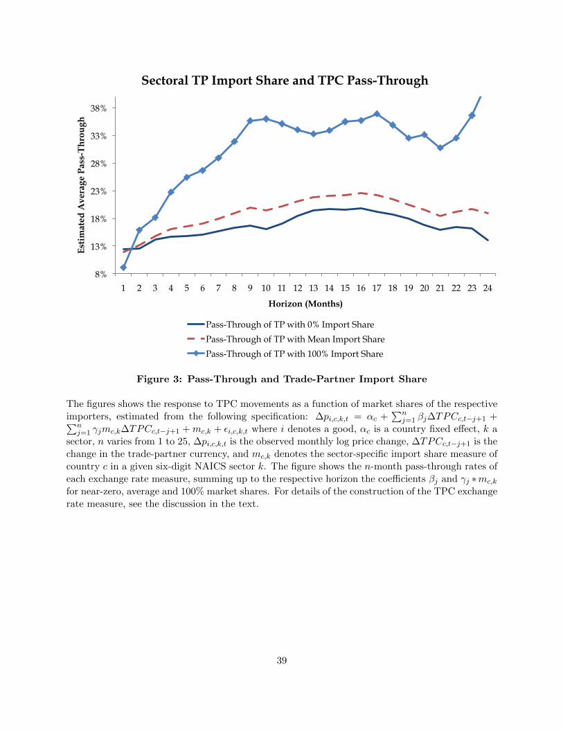
8%

13%

18%

23%

28%

33%

38%

1 2 3 4 5 6 7 8 9 10 11 12 13 14 15 16 17 18 19 20 21 22 23 24

Est

ima

ted

Av

era

ge P

ass

-Th

rou

gh

Horizon (Months)

Sectoral TP Import Share and TPC Pass-Through

Pass-Through of TP with 0% Import Share

Pass-Through of TP with Mean Import Share

Pass-Through of TP with 100% Import Share

Figure 3: Pass-Through and Trade-Partner Import Share

The figures shows the response to TPC movements as a function of market shares of the respectiveimporters, estimated from the following specification: ∆pi,c,k,t = αc +

∑nj=1 βj∆TPCc,t−j+1 +∑n

j=1 γjmc,k∆TPCc,t−j+1 +mc,k + εi,c,k,t where i denotes a good, αc is a country fixed effect, k asector, n varies from 1 to 25, ∆pi,c,k,t is the observed monthly log price change, ∆TPCc,t−j+1 is thechange in the trade-partner currency, and mc,k denotes the sector-specific import share measure ofcountry c in a given six-digit NAICS sector k. The figure shows the n-month pass-through rates ofeach exchange rate measure, summing up to the respective horizon the coefficients βj and γj ∗mc,k

for near-zero, average and 100% market shares. For details of the construction of the TPC exchangerate measure, see the discussion in the text.

39

Figure 4: Kernel Density of Actual and Predicted Price Changes and Benchmark

The figure shows the distribution of observed log price changes and log price changes predicted byour model as described in Section 4.1 in the text. As a benchmark, we also show log price changesgenerated by a constant mark-up model. Price changes are monthly log price differences, and thedistribution is truncated above 10% and below −10%.

40

Figure 5: Estimated and Predicted TPC Pass-Through, Sector-Trade Partner Pairs

The figure shows estimated and predicted pass-through rates, at the sector-TP level. Pass-throughis estimated from the following specification: ∆pi,c,t = αc +

∑nj=1 β

TPCj TPCc,t−j+1 + εi,c,t where i

denotes a good, αc is a country fixed effect, k a sector defined at the NAICS2 level, ∆pi,c,t is theobserved monthly log price change, and TPCc,t−j+1 the TPC movement. The figure shows the sumof estimated coefficients

∑24j=0 βj for each sector-TP combination. For details of the construction of

the exchange rate measures, see the discussion in the text. Predicted pass-through is the two-digitNAICS sectoral mean of pass-through predicted as in Section 4.1 in the text.

41

Figure 6: Estimated and Predicted Pass-Through, Country-Level

The figure shows estimated and predicted pass-through rates, aggregated to the country level. Pass-through is estimated from the following specification: ∆pi,c,t = αc+

∑nj=1 β

TPCj ∆TPCc,t−j+1 +εi,c,t

where i denotes a good, αc is a country fixed effect, k a sector defined at the NAICS2 level, ∆pi,c,tis the observed monthly log price change, and ∆TPCc,t−j+1 the TPC movement. The figure showsthe sum of estimated coefficients

∑24j=0 βj averaged over sectors for each country. For details of the

construction of the exchange rate measures, see the discussion in the text. Predicted pass-throughis the two-digit NAICS sectoral mean of pass-through predicted as described in Section 4.1 in thetext, averaged over sectors for each country.

42

Tab

le1:

Pre

dic

ted

an

dA

ctu

al

Pri

ce

Ch

an

ges

for

TP

CM

ovem

ents

(1)

(2)

(3)

(4)

(5)

(6)

(7)

(8)

(9)

ρ10

BW

1010

BW

1010

BW

10C

omp

etit

ion

atN

AIC

S6

Com

pet

itio

nat

NA

ICS

6C

omp

etit

ion

atH

S10

Un

con

dit

ion

al

∆p:

(1)-

(3)

Con

dit

ion

al

∆p:

(4)-

(9)

Pre

dic

ted

24-m

onth

0.09

80.

090

0.09

80.

423

0.49

30.

763

0.44

10.

567

0.65

2p

rice

chan

ge(0

.018

)(0

.016

)(0

.024

)(0

.100

)(0

.099

)(0

.165

)(0

.143

)(0

.151

)(0

.197

)

Diff

eren

tiat

edG

ood

s?-

-Y

es-

-Y

es-

-Y

es

N49

399

4357

023

868

8166

6113

2987

5125

3196

2223

R2

0.60

%0.

96%

1.05

%3.

78%

7.52

%11

.15%

4.37

%8.

29%

9.16

%

This

table

sum

mari

zes

resu

lts

from

the

follow

ing

regre

ssio

nsp

ecifi

cati

on:

∆pi,t

=αi

+∑ 24 j

βj∆pi,t−j

+ε i,t

wher

e∆pi,t

den

ote

sth

em

ean

obse

rved

log

pri

cech

ange

at

the

HS10-T

Ple

vel

,∆pi,t

the

mea

npre

dic

ted

log

pri

cech

ange

at

the

HS10-T

Ple

vel

due

toT

PC

mov

emen

tsandαi

fixed

effec

tsat

the

HS10-T

Ple

vel

.T

he

table

show

ses

tim

ate

sand

standard

erro

rsof∑ 24 j

βj.

Pre

dic

tions

are

gen

erate

dusi

ng

diff

eren

tva

lues

ofρ,

the

elast

icit

yof

subst

ituti

on

bet

wee

ngoods.

BW

indic

ate

sth

atρ

ista

ken

from

Bro

da

and

Wei

nst

ein

(2006).

Est

imate

sin

colu

mns

(4)-

(9)

are

condit

ional

on

obse

rvin

gact

ual

pri

cech

anges

while

colu

mns

(1)-

(3)

dis

pla

yunco

ndit

ional

esti

mate

s.

43

Tab

le2:

Pre

dic

ted

an

dA

ctu

al

Pri

ce

Ch

an

ges

for

US

DM

ovem

ents

(1)

(2)

(3)

(4)

(5)

(6)

(7)

(8)

(9)

ρ10

BW

1010

BW

1010

BW

10C

omp

etit

ion

atN

AIC

S6

Un

con

dit

ion

al

∆p:

(1)-

(3)

Con

dit

ion

al

∆p:

(4)-

(9)

Pre

dic

ted

24-m

onth

0.2

070.

182

0.16

91.

086

1.05

91.

223

1.18

81.

007

1.37

9p

rice

chan

ge(U

SD

bas

ed)

(0.0

37)

(0.0

35)

(0.0

45)

(0.2

28)

(0.2

22)

(0.3

27)

(0.2

41)

(0.2

19)

(0.3

29)

Pre

dic

ted

24-m

onth

0.31

40.

282

0.91

0p

rice

chan

geT

PC

bas

ed)

(0.1

25)

(0.1

14)

(0.2

12)

Diff

eren

tiat

edG

ood

s?-

-Y

es-

-Y

es-

-Y

es

N34

111

3279

016

522

1766

747

0922

0651

7747

1022

45R

20.4

6%0.

47%

0.33

%0.

68%

4.96

%8.

55%

7.99

%11

.09%

18.7

5%

This

table

sum

mari

zes

resu

lts

from

the

follow

ing

two

regre

ssio

nsp

ecifi

cati

ons:

∆pi,t

=αi+∑ 24 j

=0βj∆pUSD

i,t−j+ε i,t

for

colu

mns

(1)-

(6)

and

∆pi,t

=αi+∑ 24 j

=0βj∆pUSD

i,t−j

+∑ 24 j

=0γj∆pTPC

i,t−j

+ε i,t

for

colu

mns

(7)-

(9)

wher

e∆pi,t

den

ote

sth

em

ean

obse

rved

log

pri

cech

ange

at

the

HS10-T

Ple

vel

,∆pUSD

i,t

(∆pTPC

i,t

)th

em

ean

pre

dic

ted

log

pri

cech

ange

at

the

HS10-T

Ple

vel

due

toU

SD

(TP

C)

mov

emen

tsandαi

fixed

effec

tsat

the

HS10-T

Ple

vel

.T

he

table

show

ses

tim

ate

sand

standard

erro

rsof∑ 24 j

=0βj

and∑ 24 j

=0γj.

Est

imati

ons

inco

lum

ns

(4)-

(9)

are

condit

ional

on

obse

rvin

gact

ual

pri

cech

anges

while

colu

mns

(1)-

(3)

dis

pla

yunco

ndit

ional

esti

mate

s.T

he

esti

mati

on

inC

olu

mns

(3),

(6),

and

(9)

furt

her

rest

rict

the

sam

ple

toth

ose

class

ified

as

diff

eren

tiate

dby

Rauch

(1999).

Pri

cepre

dic

tions

ass

um

efo

rth

eel

ast

icit

yof

subst

ituti

onρ

am

ong

goods

thatρ

=10

in(1

),(3

),(4

),(6

),(7

)and

(9),

while

the

sect

or

spec

ific

esti

mate

dfr

om

Bro

da

and

Wei

nst

ein

(2006)

isuse

doth

erw

ise.

All

pri

cech

anges

ass

um

eth

at

firm

sco

mp

ete

wit

hin

six-d

igit

NA

ICS

sect

ors

and

that

imp

ort

ers

do

not

com

pet

ew

ith

dom

esti

cfirm

s.

44

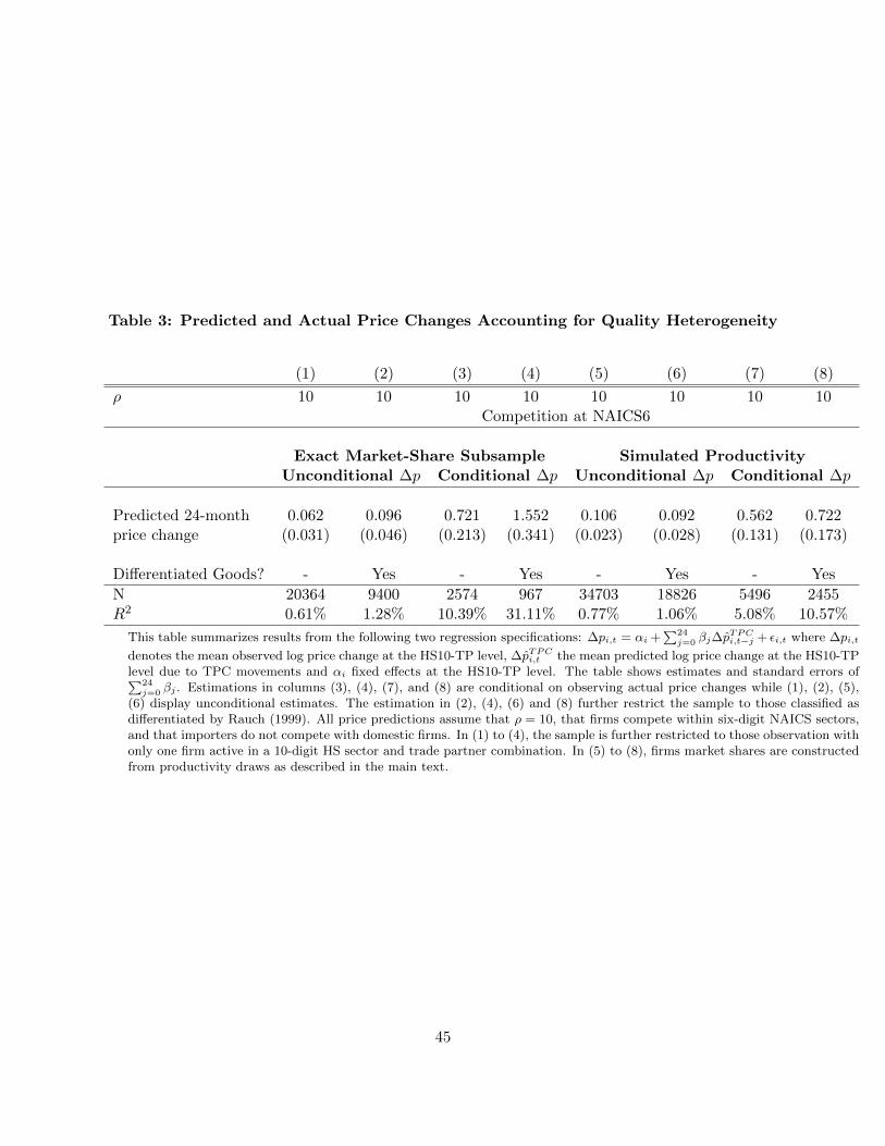
Table 3: Predicted and Actual Price Changes Accounting for Quality Heterogeneity

(1) (2) (3) (4) (5) (6) (7) (8)

ρ 10 10 10 10 10 10 10 10Competition at NAICS6

Exact Market-Share Subsample Simulated ProductivityUnconditional ∆p Conditional ∆p Unconditional ∆p Conditional ∆p

Predicted 24-month 0.062 0.096 0.721 1.552 0.106 0.092 0.562 0.722price change (0.031) (0.046) (0.213) (0.341) (0.023) (0.028) (0.131) (0.173)

Differentiated Goods? - Yes - Yes - Yes - Yes

N 20364 9400 2574 967 34703 18826 5496 2455R2 0.61% 1.28% 10.39% 31.11% 0.77% 1.06% 5.08% 10.57%

This table summarizes results from the following two regression specifications: ∆pi,t = αi +∑24j=0 βj∆p

TPCi,t−j + εi,t where ∆pi,t

denotes the mean observed log price change at the HS10-TP level, ∆pTPCi,t the mean predicted log price change at the HS10-TPlevel due to TPC movements and αi fixed effects at the HS10-TP level. The table shows estimates and standard errors of∑24j=0 βj . Estimations in columns (3), (4), (7), and (8) are conditional on observing actual price changes while (1), (2), (5),

(6) display unconditional estimates. The estimation in (2), (4), (6) and (8) further restrict the sample to those classified asdifferentiated by Rauch (1999). All price predictions assume that ρ = 10, that firms compete within six-digit NAICS sectors,and that importers do not compete with domestic firms. In (1) to (4), the sample is further restricted to those observation withonly one firm active in a 10-digit HS sector and trade partner combination. In (5) to (8), firms market shares are constructedfrom productivity draws as described in the main text.

45

Tab

le4:

Pre

dic

ted

an

dA

ctu

al

Pri

ce

Ch

an

ges

for

TP

CM

ovem

ents

,D

isse

cti

ng

the

Vari

ati

on

(1)

(2)

(3)

(4)

(5)

(6)

(7)

(8)

(9)

(10)

ρ10

1010

1010

1010

1010

10C

omp

etit

ion

atN

AIC

S6

Un

con

dit

ion

al

∆p:

(1)-

(5)

Con

dit

ion

al

∆p:

(6)-

(10)

Pre

dic

ted

24-m

onth

0.10

50.

091

0.09

70.

111

0.09

30.

612

0.38

20.

425

0.62

60.

410

pri

cech

ange

(0.0

14)

(0.0

14)

(0.0

18)

(0.0

14)

(0.0

15)

(0.0

82)

(0.0

86)

(0.1

00)

(0.0

85)

(0.0

94)

Tra

de

Part

ner

FE

Yes

--

--

Yes

--

--

Sec

tor

FE

-Y

es-

--

-Y

es-

--

Mon

thF

E-

-Y

es-

--

-Y

es-

-T

P-M

onth

FE

--

-Y

es-

--

-Y

es-

Sec

tor-

Month

FE

--

--

Yes

--

--

Yes

N493

99

4939

949

399

4939

949

399

8166

8166

8166

8166

8166

R2

0.8

8%4.

29%

0.68

%2.

31%

29.6

2%4.

53%

20.1

5%4.

29%

10.8

4%54

.76%

This

table

sum

mari

zes

resu

lts

from

the

follow

ing

regre

ssio

nsp

ecifi

cati

on:

∆pi,t

=∑ 24 j

=0βj∆pi,t−j

+FEs

+ε i,t

wher

e∆pi,t

den

ote

sth

em

ean

obse

rved

log

pri

cech

ange

at

the

HS10-T

Ple

vel

,∆pi,t

the

mea

npre

dic

ted

log

pri

cech

ange

at

the

HS10-T

Ple

vel

due

toT

PC

mov

emen

ts,

andFE

sva

rious

fixed

effec

ts.

The

table

show

ses

tim

ate

sand

standard

erro

rsof∑ 24 j

=0βj.

Est

imati

ons

inco

lum

ns

(5)-

(10)

are

condit

ional

on

obse

rvin

gact

ual

pri

cech

anges

while

colu

mns

(1)-

(5)

dis

pla

yunco

ndit

ional

esti

mate

s.C

olu

mns

(1)

and

(6)

add

trade-

part

ner

fixed

effec

ts,

(2)

and

(7)

use

fixed

effec

tsfo

rH

S6

sect

or

codes

.C

olu

mns

(3)

and

(8)

contr

ol

for

seaso

nality

.C

olu

mns

(4)

and

(9)

contr

ol

for

seaso

nality

spec

ific

totr

ade-

part

ner

sw

hile

colu

mns

(5)

and

(10)

contr

ol

for

seaso

nality

inH

S6

sect

ors

.A

llpri

cepre

dic

tions

ass

um

eth

atρ

=10,

that

firm

sco

mp

ete

wit

hin

six-d

igit

NA

ICS

sect

ors

,and

that

imp

ort

ers

do

not

com

pet

ew

ith

dom

esti

cfirm

s.

46

Tab

le5:

Pre

dic

ted

an

dA

ctu

al

Pri

ce

Ch

an

ges,

Rob

ust

ness

(1)

(2)

(3)

(4)

(5)

(6)

(7)

(8)

ρ10

1010

1010

1010

10C

omp

etit

ion

wit

hD

omes

tic

Fir

ms

Excl

ud

ing

Com

mod

ity

Exp

orte

rs

Un

con

dit

ion

al

∆p

Con

dit

ion

al

∆p

Un

con

dit

ion

al

∆p

Con

dit

ion

al

∆p

Pre

dic

ted

24-

mon

th0.

108

0.10

20.

566

0.88

60.

113

0.12

10.

560

0.92

8p

rice

chan

ge(0

.019

)(0

.026

)(0

.117

)(0

.195

)(0

.019

)(0

.027

)(0

.103

)(0

.170

)D

iffer

enti

ated

Good

s?-

Yes

-Y

es-

Yes

-Y

es

N34

316

1786

550

9522

2535

188

1626

960

2322

96R

20.

79%

1.25

%5.

71%

12.5

9%0.

86%

1.60

%5.

63%

14.9

3%

This

table

sum

mari

zes

resu

lts

from

the

follow

ing

two

regre

ssio

nsp

ecifi

cati

ons:

∆pi,t

=αi+∑ 24 j

=0βj∆pTPC

i,t−j

+ε i,t

wher

e∆pi,t

den

ote

sth

em

ean

obse

rved

log

pri

cech

ange

at

the

HS10-T

Ple

vel

,∆pTPC

i,t

the

mea

npre

dic

ted

log

pri

cech

ange

at

the

HS10-T

Ple

vel

due

toT

PC

mov

emen

tsandαi

fixed

effec

tsat

the

HS10-T

Ple

vel

.T

he

table

show

ses

tim

ate

sand

standard

erro

rsof

∑ 24 j=

0βj.

Pre

dic

tions

are

gen

erate

dusi

ng

diff

eren

tva

lues

ofρ,

the

elast

icit

yof

subst

ituti

on

am

ong

goods.

Est

imati

ons

inco

lum

ns

(3),

(4),

(7),

and

(8)

are

condit

ional

on

obse

rvin

gact

ual

pri

cech

anges

while

(1),

(2),

(5),

(6)

dis

pla

yunco

ndit

ional

esti

mate

s.T

he

esti

mati

on

in(2

),(4

),(6

)and

(8)

furt

her

rest

rict

the

sam

ple

toth

ose

class

ified

as

diff

eren

tiate

dby

Rauch

(1999).

All

pri

cepre

dic

tions

ass

um

eth

atρ

=10

and

that

firm

sco

mp

ete

wit

hin

six

dig

itN

AIC

Sse

ctors

.(1

)to

(4)

ass

um

eth

at

imp

ort

ers

do

com

pet

ew

ith

dom

esti

cfirm

sw

hile

(5)

to(8

)th

at

imp

ort

ers

do

not

com

pet

ew

ith

dom

esti

cfirm

s.(5

)to

(8)

excl

ude

all

goods

from

Canada,

Chin

a,

Norw

ayand

New

Zea

land.

47

A APPENDIX: Proofs of Proposition 1 and 2

A.1 Proposition 1

Proof. The change in the sectoral price level Pk can be solved for by acknowledging that Pk itselfis the sum of all individual prices changes (10) weighted by the firm’s market share sj,k:

Pk =∑jεNk

sjγj,kPk +∑jεNk

sjαj,kwj,k (21)

That is, the change in the general price level Pk depends on the total first round effect of how eachfirm responds to changing costs (reflected by the second summation in (21)) and on second-roundeffects: all prices depend on the general price level, which multiplies the first-round effect. Then,solving for the equilibrium price yields

Pk =∑jεNk

sjαj,kwj,k︸ ︷︷ ︸1st Round Total Direct Cost Effect

/ 1−∑jεNk

sjγj,k

︸ ︷︷ ︸

Higher Round Multiplier

. (22)

Substitution into (10) directly gives the rate of price changes as a function of the fundamental costchanges.

The solution to the recursive system of individual prices (10) is surprisingly simple. The reasonfor this simplicity is that the price of any firm n reacts linearly to the linear composition of otherprices Pk =

∑jεN sjPj,k as the preferences are additively linear within nest k.

A.2 Proposition 2

Proof. First, note that the change of the general price index is simply Pk = nUSPUS + nTP PTP +nROW PROW , and that the price of a firm from country c ∈ {US, TP,ROW} is equal to

Pc,k = Γ(Pk − Pc,k

)+ wc,k. (23)

Solving the system of three pricing equations (11) for the case of equal-sized firms yields thefollowing optimal price response for a firm originating from country n:

Pn,k = αγ

∑jεNk

sj∆ec,t

1− γ+ α∆ec,t + εn,k.

Then, remembering our definitions of the exchange rate decomposition in (2), a TPC movementof a trade partner TP implies that ∆USDROW−c,t = 0 and ∆TPCc,t 6= 0. To relate this toour empirical approach of identifying cost pass-through, we write wUSD = ∆USDROW−c,t andw′TPC ≡ ∆TPCc,t − ∆USDROW−c,t yielding the TPC price change for the case of equally sizedfirms:

PTPC,c = γ1

1− γnTPα∆TPCc,t︸ ︷︷ ︸

Effect of TPC on Pk

+ α∆TPCc,t︸ ︷︷ ︸DirectCost Effect

+ εn,k. (24)

48

where TPC pass-through is given by the sum of coefficients multiplying ∆TPCc,t.Second, remembering the price response to broad USD shock defined as in Equation (1), as well

as the fact that all prices are denominated in dollars so that the wage change of US firms is equalto 0 by definition, a USD movement implies that ∆USDROW−c,t = ∆TPCc,t, while

PUSD,c = γ1

1− γ(nROW + nTP )α∆USDROW−c,t︸ ︷︷ ︸

Effect of USD on Pk

+ α∆USDROW−c,t︸ ︷︷ ︸DirectCost Effect

+ εn,k. (25)

where USD pass-through is again given by the sum of coefficients multiplying ωUSD.The remainder of the proofs follows directly from taking derivatives of the pass-through expres-

sions. For item 2. in the proposition, note that 1− nUS = nTP + nROW .

B APPENDIX: Data description

We use exchange rates and inflation data from the IMF’s International Financial Statistics database,and, most importantly, import prices at the good level from the BLS. The latter micro price datahave been the topic of intense study since the original analysis of this dataset by Gopinath andRigobon (2008).

We refer the reader to Gopinath and Rigobon (2008) for a detailed description of the US importprice micro data. In this paper, we analyze the years from 1994 through 2005. We apply our analysisto the following countries: Austria, Canada, China, Denmark, Czech Republic, Finland, France,Germany, Greece, Hungary, Ireland, Italy, Japan, Mexico, Netherlands, New Zealand, Norway,Portugal, Singapore, South Korea, Spain, Sweden, Switzerland, Taiwan, United Kingdom.

In manipulating the data, we follow the main steps taken in Gopinath and Rigobon (2008). Inparticular, we drop net price data which are flagged by the BLS as not usable, not index usable orfor which a price has been estimated. There are 771872 usable prices in our sample. In addition,we pull forward a last observed price when a price is missing as in Nakamura and Steinsson (2012).We also disregard an entire price series if more than 10% of prices of a series have been flagged asprice records with no trade. All of our prices are market price transactions invoiced in USD.22

To construct trade partner market shares, we use bilateral US import data from the US Census,disaggregated at either the six-digit Harmonized System (HS) or the six-digit North AmericanIndustry Classification System (NAICS). To construct measures of the openness of a sector, werequire data on domestic sales in addition to imports. We use data on the shipments of domesticfirms recorded in the Annual Survey of Manufacturers, which is available from the US census atthe six-digit NAICS level.

C APPENDIX: Additional Figures and Tables

Is the fact that TPC currency is low driven by specific trade partners? In Table C.2, weestimate the PT rate jointly following USD and TPC movements for each of the countries in oursample separately and at the 6 and 12-months horizons. These estimations unveil a large degree in

22As Gopinath and Rigobon (2008) have documented, almost all US imports are priced in USD. For example,93.4% of all import prices are in USD in 2004. Neiman (2010) explicitly studies the behavior of intra-firm priceswhich account for approximately 40% of the data.

49

heterogeneity, with the TPC PT rate varying from 17% to 68% and the USD PT rate varying from16% to 90%. However, it is both true that the median and the mean TPC rate are statisticallylower than the mean and median of the USD rate. Moreover, it is also true that for 16 out of the23 trade partners, TPC pass-through is estimated to be higher than USD pass-through.

Is the difference in PT rates following TPC and USD movements driven by specificsectors? We next estimate disaggregate pass-through regressions within 3−digit NAICS sectors(we do not have enough data points for estimating PT rates within finer disaggregations). FigureC.1 displays the PT rates at the 1-24 month(s) horizons for two selected industries (NAICS 314“Textile product mills”, blue lines and 325 “Chemical Manufacturing”, red lines). In both sectors,the TPC PT rate (dashed lines) is markedly below the USD PT rate (solid line).

To run the same robustness check for all 3-digit NAICS industries, Figure C.2 next presentsa scatter plot relating the USD PT rate to the TPC PT rate. In this diagram, the vertical axisdisplays the estimated sector-specific USD PT rate. The horizontal axis presents the TPC PT rate.In Figure C.2, each datapoint then displays the TPC and the USD PT rate in one sector and atthe 12-month time horizon. Figure C.2 also plots the 45 degree line. The majority of observationsare above this line, hence indicating that USD PT is indeed higher one average than the TPC PTrate. Also a fitted line is estimated above the 45 degree line.

These robustness checks confirm that pass-through of broad USD movements is larger thantrade-partner or nominal exchange rate pass-through also at the country and three-digit NAICSlevel. Broad USD movements are passed through into U.S. import prices at a substantially higherrate than trade-partner movements.

Table C.1: Nominal vs USD or Trade Partner Pass-Through Rates

(1) (2) (3) (4) (5)

NOM USD TPC USD TPCSample: (1)-(3) All Observations, Single Estimation (4)-(5) Full sample, joint estimation

Horizon

1 5.75% 18.92% 3.44% 19.81% 4.09%3 8.63% 23.72% 5.58% 25.28% 6.55%6 10.91% 31.16% 7.23% 32.96% 8.06%12 14.18% 39.94% 8.63% 40.69% 9.16%18 16.33% 41.58% 10.21% 41.39% 10.15%24 15.11% 31.59% 7.34% 29.67% 9.73%

The table shows estimates of PT for nominal bilateral, TPC and USD movements, as shown in Figures 1 and2. The estimated specification for (1)-(3) is ∆pi,c,t = αc +

∑nj=1 βj∆ec,t−j+1 +

∑nj=1 γ

TPj ∆πTPc,t−j+1 + εi,c,t

where i indexes goods, c trade partners, αc is a country fixed effect, n measures the length of the pass-throughhorizon, and ∆ec,t−j+1 is the monthly change in either the log of the nominal, USD, or TPC exchange rate.Details of the exchange rate decomposition are in the discussion in the text. ∆πTPc,t−j+1 is the monthlyinflation rate in the foreign country using the consumer price index. The estimated specification for (4)-(5)is ∆pi,c,t = αc +

∑nj=1 β

USDj ∆USDROW−c,t−j+1 +

∑nj=1 β

TPCj ∆TPCc,t−j+1 +

∑nj=1 γj∆π

TPc,t−j+1 + εi,c,t

where ∆TPCc,t−j+1 corresponds to TPC movements and ∆USDROW−c,t−j+1 to the USD movements of theexchange rate of country c.

50

Table C.2: Trade-Partner and USD Exchange Rate Pass-Through by Country

TPC USD TPC USD

Country/Horizon 6 months 12 months

Canada 16% 37% 32% 54%Mexico 2% 18% 5% -1%Sweden 10% 37% 18% 54%Norway 16% 61% 20% 63%Finland 7% 26% 13% 36%Denmark 18% 43% 23% 39%UK 4% 56% -44% 75%Ireland 1% -9% 16% -9%Netherlands -4% 87% 14% 90%France 17% 12% 18% 5%Germany 51% 31% 56% 34%Austria 24% 34% 30% 62%Czech 8% 17% 10% 77%Hungary -17% 90% 1% 69%Switzerland 56% 52% 59% 52%China 8% -16% 24% -22%Portugal 25% 47% 43% 72%Italy 27% 32% 37% 36%Greece -1% 10% 7% 21%Singapore 68% 20% 53% 36%Korea 2% 24% 9% 39%Japan 29% 4% 46% -10%New Zealand 21% 55% 10% 53%

Mean 24% 37% 30% 51%Median 25% 34% 29% 50%

The table shows country-specific estimates of PT forTPC and USD movements. The estimated specifi-cation is ∆pi,c,t =

∑nj=1 β

USDj ∆USDROW−c,t−j+1 +∑n

j=1 βTPCj ∆TPCc,t−j+1 +

∑nj=1 γj∆π

TPc,t−j+1 + εi,c,t where

i indexes goods, c trade partners and n measures the length ofthe pass-through horizon with n ∈ (6, 12). Details of the exchangerate decomposition are in the discussion in the text. ∆pi,c,t is theobserved monthly log price change, and ∆πTPc,t−j+1 is the monthlyinflation rate in the foreign country using the consumer priceindex. The table reports the sum of the estimated coefficients βijat 6 and 12 month horizons for i ∈ (USD, TPC).

51

-5

0

5

10

15

20

1 2 3 4 5 6 7 8 9 10 11 12 13 14 15 16 17 18 19 20 21 22 23 24

Est

imate

d P

ass

-Th

rou

gh

Horizon in Months

Pass-Through of USD and TPC Movements for Two Selected Industries

314 TPC PT 314 USD PT 325 TPC PT 325 USD PT

Figure C.1: Pass-Through for TP and USD Movements for NAICS Industries 314 and325

The figures shows estimates of TPC and USD pass-through for two specific sectors from the fol-lowing specification ∆pi,c,t = αc +

∑nj=1 β

TPCj TPCc,t−j+1 +

∑nj=1 β

USDj USDc,t−j+1 + εi,c,t where

i denotes a good, αc is a country fixed effect, either 314 or 325, ∆pi,c,t is the observed monthlylog price change, and TPCc,t−j+1 and USDc,t−j+1 TP and USD movements. The figure shows thesum of the coefficients

∑nj=0 βj estimated for each exchange rate measure and each sector at each

horizon. For details of the construction of the exchange rate measures, see the discussion in thetext.

52

-30.00%

-20.00%

-10.00%

0.00%

10.00%

20.00%

30.00%

40.00%

50.00%

60.00%

70.00%

-30.00% -20.00% -10.00% 0.00% 10.00% 20.00% 30.00% 40.00% 50.00% 60.00% 70.00%

Est

imate

d T

PC

Pass

-Th

rou

gh

Estimate USD Pass-Through

USD versus TPC Pass-Through Rates at the Sectoral Level

Figure C.2: USD versus TPC Pass-Through Rates at the Sectoral Level

The figures shows estimates of TPC and USD pass-through by sector from the following specification∆pi,c,t = αc +

∑24j=1 βjec,t−j+1 + εi,c,t where i denotes a good, αc is a country fixed effect, ∆pi,c,t is

the observed monthly log price change, and ec,t−j+1 denotes TPC or USD movements. The figureshows the sum of the coefficients

∑24j=0 βj estimated for each NAICS3 sector and exchange rate

movement. For details of the construction of the exchange rate measures, see the discussion in thetext.

53

Table C.3: Long-Run Price Change Regressions

(1) (2) (3)

ρ 10 BW 10Competition at NAICS6

Predicted Price Changes 0.298 0.235 0.271(0.114) (0.121) (0.155)

Differentiated Goods? - - Yes

N 6156 6156 2656R2 13.47% 12.83% 16.82%

The table shows estimates of long-run pass-through from thefollowing specification: ∆pLRi = αi + βLR∆pLRi + εi where∆pLRi denotes the log price change over the entire life-time of agood, ∆pLRi the corresponding predicted log price change andαi good-level fixed effects. The table shows estimates βLR andtheir standard errors in brackets.

54