market liquidity: proceedings of workshop held at the bis ... · market microstructure refers to...
TRANSCRIPT
BIS Papers No 2
Market liquidity: proceedings of workshop held at the BIS
Monetary and Economic Department
April 2001

Papers in this volume were prepared for a meeting held at the Bank for International Settlements on 7 August 2000. The views expressed are those of the authors and do not necessarily reflect the views of the BIS or the central banks represented at the meeting. Individual papers (or excerpts thereof) may be reproduced or translated with the authorisation of the authors concerned.
Requests for copies of publications, or for additions/changes to the mailing list, should be sent to:
Bank for International Settlements Information, Press & Library Services CH-4002 Basel, Switzerland E-mail: [email protected]
Fax: (+41 61) 280 9100 and (+41 61) 280 8100
This publication is available on the BIS website (www.bis.org).
© Bank for International Settlements 2001. All rights reserved.
ISSN 1609-0381
ISBN 92-9131-619-9

BIS Papers No 2 i
Table of contents
List of workshop participants ............................................................................................................. iii
Session I - Stock marketsOverview: market structure issues in market liquidity:Maureen OHara (Cornell University) ................................................................................................. 1
Events that shook the market:Ray C Fair (Yale University) .............................................................................................................. 9
Comments:Eloy Lindeijer (De Nederlandsche Bank) ........................................................................... 25Giuseppe Grande (Banca d'Italia) ...................................................................................... 27
Information flows during the Asian crisis: evidence from closed-end funds:Benjamin H Cohen and Eli M Remolona (Bank for International Settlements) ................................. 30
Comments:Tatsuya Yonetani (Bank of Japan) ..................................................................................... 71Torben G Andersen (Northwestern University) .................................................................. 73
Session II - Bond marketsEstimating liquidity premia in the Spanish Government securities market:Francisco Alonso, Roberto Blanco, Ana del Río and Alicia Sanchís (Banco de España) ................. 79
Comments:Christian Upper (Deutsche Bundesbank) ........................................................................... 108Oreste Tristani (European Central Bank) ........................................................................... 110
Does market transparency matter? A case study:Antonio Scalia and Valerio Vacca (Banca d'Italia) ............................................................................. 113
Comments:Agnes Van den Berge (Banque Nationale de Belgique) .................................................... 141Peter Rappoport (JP Morgan) ............................................................................................ 143
Special session - Panel discussionShort introduction on the work of the Johnson group:Eloy Lindeijer (De Nederlandsche Bank) ........................................................................................... 147
Market liquidity under stress: observations from the FX market:Francis Breedon (Lehman Brothers) ................................................................................................. 149
The puzzling decline in financial market liquidity:Avinash Persaud (State Street) ......................................................................................................... 152
Measuring liquidity under stress:Christian Upper (Deutsche Bundesbank) .......................................................................................... 159
Session III - Foreign exchange marketsOrder flow and exchange rate dynamics:Martin D D Evans (Georgetown) and Richard K Lyons (University of California, Berkley) ............... 165
Comments:Eric Jondeau (Banque de France) ..................................................................................... 192Robert N McCauley (Bank for International Settlements) .................................................. 194

ii BIS Papers No 2
Trading volumes, volatility and spreads in FX markets: evidence from emerging market countries:Gabriele Galati (Bank for International Settlements) ......................................................................... 197
Comments:Javiera Ragnartz (Sveriges Riksbank) ............................................................................... 226Alain Chaboud (Federal Reserve System) ......................................................................... 229
Other papersSending the herd off the cliff edge: the disturbing interaction between herding andmarket-sensitive risk management practices:Avinash Persaud (State Street) ......................................................................................................... 233
How safe was the Safe Haven? Financial market liquidity during the 1998 turbulences:Christian Upper (Deutsche Bundesbank) .......................................................................................... 241
FX impact of cross-border M&A:Francis Breedon and Francesca Fornasari (Lehman Brothers) ........................................................ 267

BIS Papers No 2 iii
Workshop on market liquidityBank for International Settlements
Basel, Switzerland7 August 2000
List of participants
Name and affiliation E-mail address
Richard AdamsCitibank N AUnited Kingdom
Laura AmbrosenoState Street Bank & Trust CompanyUnited Kingdom
Torben G AndersenNorthwestern UniversityUnited States
Peter BartkoEBS PartnershipUnited Kingdom
Florence Béranger1
Bank for International SettlementsSwitzerland
Roberto BlancoBanco de EspañaSpain
Claudio BorioBank for International SettlementsSwitzerland
Francis BreedonLehman BrothersUnited Kingdom
Martin BrookeBank of EnglandUnited Kingdom
Alain ChaboudBoard of Governors of the Federal Reserve SystemUnited States
Benjamin CohenBank for International SettlementsSwitzerland
Chris D'SouzaBank of CanadaCanada

iv BIS Papers No 2
Name and affiliation E-mail address
Ray FairYale UniversityUnited States
Gabriele GalatiBank for International SettlementsSwitzerland
Giuseppe GrandeBanca d'ItaliaItaly
Stefan HohlDeutsche BundesbankGermany
Eric JondeauBanque de FranceFrance
Michael LewisDeutsche BankUnited Kingdom
Eloy LindeijerDe Nederlandsche BankThe Netherlands
Richard LyonsUniversity of CaliforniaUnited States
Robert McCauleyBank for International SettlementsHong Kong SAR
Maureen O'HaraCornell UniversityUnited States
Avinash PersaudState Street Bank & Trust CompanyUnited Kingdom
Javiera RagnartzSveriges RiksbankSweden
Peter RappoportJ P Morgan Securities, Inc.United States
Eli RemolonaBank for International SettlementsSwitzerland
Marcel Savioz [email protected]

BIS Papers No 2 v
Name and affiliation E-mail addressSchweizerische NationalbankSwitzerland
Antonio ScaliaBanca d'ItaliaItaly
Oreste TristaniEuropean Central BankGermany
Christian UpperDeutsche BundesbankGermany
Agnes Van den BergeBanque Nationale de BelgiqueBelgium
Philip WooldridgeBank for International SettlementsSwitzerland
Tatsuya YonetaniBank of JapanJapan
1 Since 1 November 2000 at CDC IXIS Capital Markets


Session IStock markets


BIS Papers No 2 1
Overview: market structure issues in market liquidityMaureen OHara1
The behaviour of prices and even the viability of markets depend on the ability of the tradingmechanism to match the trading desires of sellers and buyers. This matching process involves theprovision of market liquidity. The role of the market maker in providing liquidity is widely recognised,but liquidity can also arise from other aspects of the trading mechanism. In particular, rules and marketpractices governing the trading process, such as how trading orders are submitted and what tradinginformation must be disclosed, can affect the creation of liquidity. This raises the question of whetherchanges in market structure can enhance the provision of liquidity. Is there a Golconda exchangethat provides optimal liquidity?
What is microstructure?Issues related to market liquidity are part of a broader analysis of the microstructure of markets.Market microstructure refers to the study of the process and outcomes of exchanging assets under aspecific set of rules. While much of economics abstracts from the mechanics of trading, microstructuretheory focuses on how specific trading mechanisms affect the price formation process.2
Much of the microstructure literature has focused on the price-setting problem confronting marketintermediaries. The Walrasian auctioneer provides the simplest (and oldest) characterisation of theprice-setting process. The auctioneer announces a potential trading range, and traders determine theiroptimal order at that price. If there are imbalances in traders demands and supplies, a new potentialprice is suggested, and traders then revise any orders. No trading takes place until a market-clearingprice is found. The London gold fixing loosely resembles the Walrasian framework, but most othermarkets differ dramatically. In particular, specific market participants play roles far removed from thepassive one of the auctioneer. Demsetz (1968) was one of the first economists to analyse how thebehaviour of traders affects the formation of prices. Demsetz argued that while a trader willing to waitmight trade at the single price envisioned in the Walrasian framework, a trader not wanting to waitcould pay a price for immediacy, ie liquidity. This results in two equilibrium prices. Moreover, since thesize of the price concession needed to trade immediately depends on the number of traders, thestructure of the market could affect the cost of immediacy and thus the market-clearing price.
The price-setting problem examined by Demsetz has been investigated more formally using inventory-based models. These models view the trading process as a matching problem in which the marketmaker - or price-setting agent - must use prices to balance supply and demand across time. There areseveral distinct approaches to modelling how prices are set by market makers: Garman (1976)focused on the nature of order flow; Stoll (1978) and Ho and Stoll (1981) examined the optimisationproblem facing dealers; and Cohen, Maier, Schwartz and Whitcomb (1981) analysed the effects ofmultiple providers of immediacy. Common to each of these approaches are uncertainties in order flow,which can result in inventory problems for the market maker and execution problems for traders.
An alternative approach to modelling the behaviour of prices focuses on the learning problemconfronting market intermediaries. Starting with Kyle (1984, 1985), Glosten and Milgrom (1985) andEasley and OHara (1987), market structure research has given greater attention to the effect ofasymmetric information on market prices. If some traders have superior information about theunderlying value of an asset, their trades could reveal what this underlying value is and so affect thebehaviour of prices.
The key to extracting information from order flows is Bayesian learning. Each trader has a prior beliefabout the true value V of an asset. Traders observe some data, say a trade, and then calculate theprobability that V equals their prior belief given that these data have been observed. This conditional
1 Johnson Graduate School of Management, Cornell University and President-elect of the American Finance Association.Special thanks to Philip Wooldridge at the Bank for International Settlements for transcribing this presentation.
2 For a survey of the literature, see OHara (1995) or Madhavan (2000). Lyons (forthcoming) provides a comprehensivereview of the microstructure of foreign exchange markets.
2 BIS Papers No 2
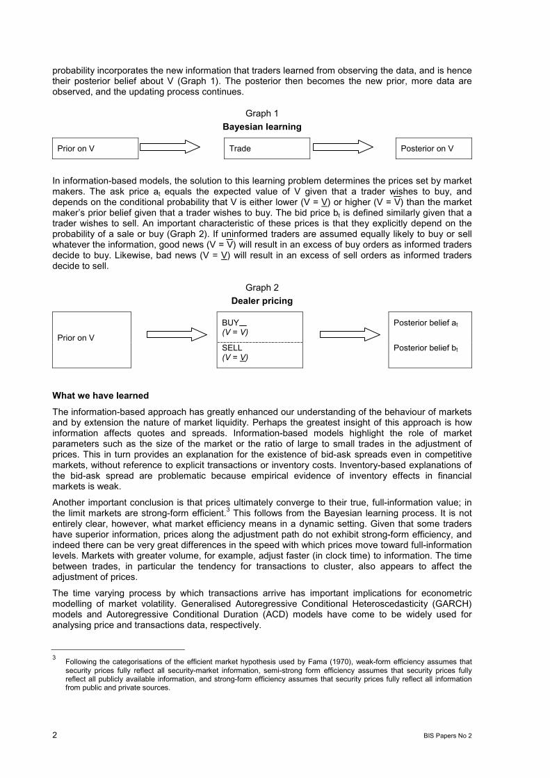
probability incorporates the new information that traders learned from observing the data, and is hencetheir posterior belief about V (Graph 1). The posterior then becomes the new prior, more data areobserved, and the updating process continues.
Graph 1Bayesian learning
Prior on V Trade Posterior on V
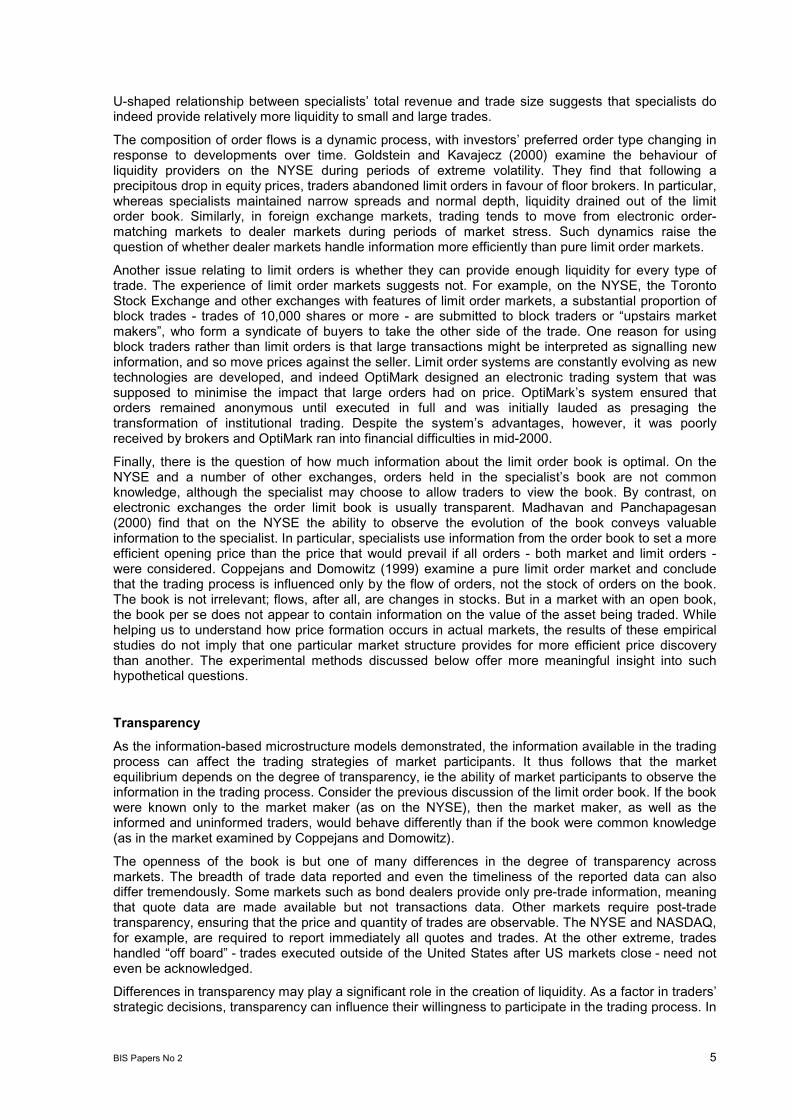
In information-based models, the solution to this learning problem determines the prices set by marketmakers. The ask price at equals the expected value of V given that a trader wishes to buy, anddepends on the conditional probability that V is either lower (V = V) or higher (V = V) than the marketmakers prior belief given that a trader wishes to buy. The bid price bt is defined similarly given that atrader wishes to sell. An important characteristic of these prices is that they explicitly depend on theprobability of a sale or buy (Graph 2). If uninformed traders are assumed equally likely to buy or sellwhatever the information, good news (V = V) will result in an excess of buy orders as informed tradersdecide to buy. Likewise, bad news (V = V) will result in an excess of sell orders as informed tradersdecide to sell.
Graph 2Dealer pricing
BUY(V = V)
Posterior belief at
Prior on VSELL(V = V)
Posterior belief bt
What we have learnedThe information-based approach has greatly enhanced our understanding of the behaviour of marketsand by extension the nature of market liquidity. Perhaps the greatest insight of this approach is howinformation affects quotes and spreads. Information-based models highlight the role of marketparameters such as the size of the market or the ratio of large to small trades in the adjustment ofprices. This in turn provides an explanation for the existence of bid-ask spreads even in competitivemarkets, without reference to explicit transactions or inventory costs. Inventory-based explanations ofthe bid-ask spread are problematic because empirical evidence of inventory effects in financialmarkets is weak.
Another important conclusion is that prices ultimately converge to their true, full-information value; inthe limit markets are strong-form efficient.3 This follows from the Bayesian learning process. It is notentirely clear, however, what market efficiency means in a dynamic setting. Given that some tradershave superior information, prices along the adjustment path do not exhibit strong-form efficiency, andindeed there can be very great differences in the speed with which prices move toward full-informationlevels. Markets with greater volume, for example, adjust faster (in clock time) to information. The timebetween trades, in particular the tendency for transactions to cluster, also appears to affect theadjustment of prices.
The time varying process by which transactions arrive has important implications for econometricmodelling of market volatility. Generalised Autoregressive Conditional Heteroscedasticity (GARCH)models and Autoregressive Conditional Duration (ACD) models have come to be widely used foranalysing price and transactions data, respectively.
3 Following the categorisations of the efficient market hypothesis used by Fama (1970), weak-form efficiency assumes thatsecurity prices fully reflect all security-market information, semi-strong form efficiency assumes that security prices fullyreflect all publicly available information, and strong-form efficiency assumes that security prices fully reflect all informationfrom public and private sources.

BIS Papers No 2 3
Finally, much has been learned about the information contained in specific trades. Different types oftrades seem to have different information content. Similarly, trades in different markets seem to havedifferent information content.
What we still do not knowFor all that we have learned, there remain several puzzling issues concerning the trading process.Foremost is what determines volume. While empirical research has identified a strong link betweenvolume and price movements, it is not obvious why this should be so. Volume may simply be aconsequence of the trading process; whereas individual trades cause prices to change, volume per semay not affect prices. Or as seems more likely, volume could reveal underlying information, and thusbe a component in the learning process. Pfleiderer (1984), Campbell et al (1991), Harris andRaviv (1993), Blume et al (1994), and Wang (1994) have examined this informational role.
A second set of issues revolves around what the uninformed traders are doing. It is the uninformedtraders who provide the liquidity to the informed, and so understanding their behaviour can providesubstantial insight and intuition into the trading process. Information-based microstructure modelstypically assume that uninformed traders do not act strategically. Yet, if it is profitable for informedtraders to time their trades, then it must be profitable for uninformed traders to do so as well. Admatiand Pfleiderer (1988, 1989), Foster and Viswanathan (1990), Seppi (1990) and Spiegel andSubrahmanyam (1992) among others have applied a game-theoretic approach to modelling thedecisions of uninformed traders. A common outcome with this approach, however, is the occurrence ofmultiple equilibria.
Another open question is what traders can learn from other pieces of market data, such as prices.Neither sequential trade models such as Glosten and Milgrom (1985) nor batch trading models suchas Kyle (1985) allow traders to learn anything from the movement of prices that is not already in theirinformation set. But in actual asset markets the price elasticity of prices appears to be important.Technical analysis of market data is widespread in markets, with elaborate trading strategies devisedto respond to the pattern of prices.
Finally, microstructure theory has not yet convincingly addressed how the existence of more than oneliquidity provider in more than one market setting affects the price adjustment process. Much of theliterature assumes the existence of a single market-clearing agent. However, alternative mechanismscould arise that divert order flow away from the specialist. Multi-market linkages introduce complexand often conflicting effects on market liquidity and trading behaviour. Indeed, it is not even obviouswhether a segmented market equilibrium is sustainable. Current models of liquidity, for example,suggest that securities markets may have an inherent disposition toward being natural monopolies.Further research in this area is particularly important given the rapid increase in the number ofelectronic exchanges in recent years.
Market structuresMarkets are currently structured in a myriad of ways, and new market-clearing mechanisms are arisingwith surprising frequency. All trading in a particular security can be directed to a single specialist, whois expected to make a market in that security. The New York Stock Exchange (NYSE) is the bestknown example of such a market structure (Table 1). Alternatively, dealers can compete for trades,buying and selling securities for their own account. Traditionally dealers competed in a centrallocation, such as the London Stock Exchange or NASDAQ, but competition need not be centralised.Bonds, for example, trade primarily through bilateral negotiations between dealers and customers. Astill third trading mechanism is the automatic matching of orders through an electronic broker. Todaythe majority of trading in the global foreign exchange market takes place over electronic exchangessuch as Reuters and Electronic Broking System (EBS).

4 BIS Papers No 2
Table 1Market structures
Specialist Dealer Electronic
Equity New York Stock Exchange NASDAQLondon Stock Exchange
Stock Exchange of Hong KongInstinetParis Bourse
Bond Bond dealers TradenetEUREX
Foreign exchange FX brokers ReutersEBS
Actual markets do not conform to simple structures. Indeed, they typically involve more than onestructure. What is important, therefore, is not the operation of any specific trading mechanism, butrather the rules by which trades occur. These rules dictate what can be traded, who can trade, whenand how orders can be submitted, who may see or handle the order, and how orders are processed.The rules determine how market structures work, and thus how prices are formed.
Since rules can affect the behaviour of prices, liquidity might also naturally depend on how a market isstructured. Indeed, liquidity concerns may dictate the structure of the market. Drawing on theextensive body of research investigating the interaction between market structure and liquidity, theremainder of this paper focuses on two critical issues in the creation of liquidity: the impact of limitorders, and the effects of transparency.
Limit ordersA wide variety of order types are found in securities markets. The most familiar type is a market orderto buy or sell one round lot at the prevailing price. Other orders, such as market-at-close, fill-or-killand immediate-or-cancel allow traders to control the timing, quantity or execution of their trades. Byfar the most common alternative type of order is a limit order specifying a price and a quantity at whicha trade is to transact. Limit orders specify a price either above the current ask or below the current bidand await the movement of prices to become active. If the market is rising, the upward pricemovement triggers limit orders to sell; if the market is falling, the downward movement triggers limitorders to buy. Limit orders thus provide liquidity to the market.
Limit order traders receive a better price than they would have if they had submitted a market order,but face the risk of non-execution and a winners curse problem. Whereas a market order executeswith certainty, limit orders await the movement of prices to become active, ie a limit order is held in abook until either a matching order is entered or the order is cancelled. Moreover, because onceposted their prices do not respond to the arrival of new information, limit orders are more likely to beexecuted when they are mispriced. Foucault (1999) finds that in deciding whether to submit a marketorder or post a limit order, traders main consideration is the volatility of an asset. In a volatile market,the probability of mispricing an asset is higher, and so limit order traders quote relatively wide bid-askspreads. This raises the cost of market order trading, thereby increasing the incentive to use limitorders rather than market orders. But as a result of fewer market orders, the execution risk associatedwith limit orders increases.
Order size may also influence investors choice between market and limit orders. Seppi (1997)concludes that small retail and large institutional investors prefer hybrid markets such as the NYSE,where specialists compete with limit orders to execute market orders.4 Mid-size investors, on the otherhand, might prefer pure limit order markets such as electronic exchanges. According to Seppi,specialists will undercut limit order prices at the margin. Such undercutting lowers the probability thatlimit orders will execute, thus resulting in reduced depth in the book. Evidence in Sofianos (1995) of a
4 In hybrid markets, the ability of limit orders to compete with market makers depends on priority rules. Limit orders to sell atprices at or below the price at which the specialist proposes to sell, or limit orders to buy at or above the specialists bidprice, typically have priority for execution.
BIS Papers No 2 5
U-shaped relationship between specialists total revenue and trade size suggests that specialists doindeed provide relatively more liquidity to small and large trades.
The composition of order flows is a dynamic process, with investors preferred order type changing inresponse to developments over time. Goldstein and Kavajecz (2000) examine the behaviour ofliquidity providers on the NYSE during periods of extreme volatility. They find that following aprecipitous drop in equity prices, traders abandoned limit orders in favour of floor brokers. In particular,whereas specialists maintained narrow spreads and normal depth, liquidity drained out of the limitorder book. Similarly, in foreign exchange markets, trading tends to move from electronic order-matching markets to dealer markets during periods of market stress. Such dynamics raise thequestion of whether dealer markets handle information more efficiently than pure limit order markets.
Another issue relating to limit orders is whether they can provide enough liquidity for every type oftrade. The experience of limit order markets suggests not. For example, on the NYSE, the TorontoStock Exchange and other exchanges with features of limit order markets, a substantial proportion ofblock trades - trades of 10,000 shares or more - are submitted to block traders or upstairs marketmakers, who form a syndicate of buyers to take the other side of the trade. One reason for usingblock traders rather than limit orders is that large transactions might be interpreted as signalling newinformation, and so move prices against the seller. Limit order systems are constantly evolving as newtechnologies are developed, and indeed OptiMark designed an electronic trading system that wassupposed to minimise the impact that large orders had on price. OptiMarks system ensured thatorders remained anonymous until executed in full and was initially lauded as presaging thetransformation of institutional trading. Despite the systems advantages, however, it was poorlyreceived by brokers and OptiMark ran into financial difficulties in mid-2000.
Finally, there is the question of how much information about the limit order book is optimal. On theNYSE and a number of other exchanges, orders held in the specialists book are not commonknowledge, although the specialist may choose to allow traders to view the book. By contrast, onelectronic exchanges the order limit book is usually transparent. Madhavan and Panchapagesan(2000) find that on the NYSE the ability to observe the evolution of the book conveys valuableinformation to the specialist. In particular, specialists use information from the order book to set a moreefficient opening price than the price that would prevail if all orders - both market and limit orders -were considered. Coppejans and Domowitz (1999) examine a pure limit order market and concludethat the trading process is influenced only by the flow of orders, not the stock of orders on the book.The book is not irrelevant; flows, after all, are changes in stocks. But in a market with an open book,the book per se does not appear to contain information on the value of the asset being traded. Whilehelping us to understand how price formation occurs in actual markets, the results of these empiricalstudies do not imply that one particular market structure provides for more efficient price discoverythan another. The experimental methods discussed below offer more meaningful insight into suchhypothetical questions.
TransparencyAs the information-based microstructure models demonstrated, the information available in the tradingprocess can affect the trading strategies of market participants. It thus follows that the marketequilibrium depends on the degree of transparency, ie the ability of market participants to observe theinformation in the trading process. Consider the previous discussion of the limit order book. If the bookwere known only to the market maker (as on the NYSE), then the market maker, as well as theinformed and uninformed traders, would behave differently than if the book were common knowledge(as in the market examined by Coppejans and Domowitz).
The openness of the book is but one of many differences in the degree of transparency acrossmarkets. The breadth of trade data reported and even the timeliness of the reported data can alsodiffer tremendously. Some markets such as bond dealers provide only pre-trade information, meaningthat quote data are made available but not transactions data. Other markets require post-tradetransparency, ensuring that the price and quantity of trades are observable. The NYSE and NASDAQ,for example, are required to report immediately all quotes and trades. At the other extreme, tradeshandled off board - trades executed outside of the United States after US markets close - need noteven be acknowledged.
Differences in transparency may play a significant role in the creation of liquidity. As a factor in tradersstrategic decisions, transparency can influence their willingness to participate in the trading process. In
6 BIS Papers No 2
the United Kingdom, for example, the Financial Services Authority allows the reporting of large tradesto be delayed for a period of time because it believes that immediate disclosure would expose marketmakers to undue risk as they unwound their positions and so discourage them from providing liquidity.Transparency is also a crucial consideration in the competition among markets for trading volume, andthus in the prospects for further fragmentation of liquidity.
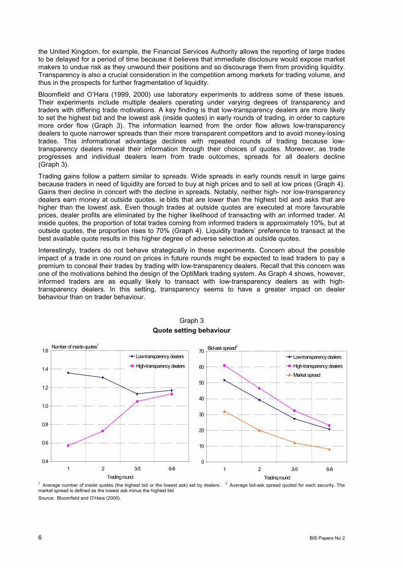
Bloomfield and OHara (1999, 2000) use laboratory experiments to address some of these issues.Their experiments include multiple dealers operating under varying degrees of transparency andtraders with differing trade motivations. A key finding is that low-transparency dealers are more likelyto set the highest bid and the lowest ask (inside quotes) in early rounds of trading, in order to capturemore order flow (Graph 3). The information learned from the order flow allows low-transparencydealers to quote narrower spreads than their more transparent competitors and to avoid money-losingtrades. This informational advantage declines with repeated rounds of trading because low-transparency dealers reveal their information through their choices of quotes. Moreover, as tradeprogresses and individual dealers learn from trade outcomes, spreads for all dealers decline(Graph 3).
Trading gains follow a pattern similar to spreads. Wide spreads in early rounds result in large gainsbecause traders in need of liquidity are forced to buy at high prices and to sell at low prices (Graph 4).Gains then decline in concert with the decline in spreads. Notably, neither high- nor low-transparencydealers earn money at outside quotes, ie bids that are lower than the highest bid and asks that arehigher than the lowest ask. Even though trades at outside quotes are executed at more favourableprices, dealer profits are eliminated by the higher likelihood of transacting with an informed trader. Atinside quotes, the proportion of total trades coming from informed traders is approximately 10%, but atoutside quotes, the proportion rises to 70% (Graph 4). Liquidity traders preference to transact at thebest available quote results in this higher degree of adverse selection at outside quotes.
Interestingly, traders do not behave strategically in these experiments. Concern about the possibleimpact of a trade in one round on prices in future rounds might be expected to lead traders to pay apremium to conceal their trades by trading with low-transparency dealers. Recall that this concern wasone of the motivations behind the design of the OptiMark trading system. As Graph 4 shows, however,informed traders are as equally likely to transact with low-transparency dealers as with high-transparency dealers. In this setting, transparency seems to have a greater impact on dealerbehaviour than on trader behaviour.
Graph 3Quote setting behaviour
Number of inside quotes1
0.4
0.6
0.8
1.0
1.2
1.4
1.6
1 2 3-5 6-8Trading round
Low-transparency dealers
High-transparency dealers
Bid-ask spread2
0
10
20
30
40
50
60
70
1 2 3-5 6-8Trading round
Low-transparency dealers
High-transparency dealers
Market spread
1 Average number of inside quotes (the highest bid or the lowest ask) set by dealers. 2 Average bid-ask spread quoted for each security. Themarket spread is defined as the lowest ask minus the highest bid.Source: Bloomfield and OHara (2000).

BIS Papers No 2 7
Graph 4Dealer gains and adverse selection
Average dealer gains1
-100
0
100
200
300
400
1 2 3-5 6-8
Trading round
Total gains of lowTotal gains of highGains of low at outsideGains of high at outside
Proportion of trades from informed traders2
0
10
20
30
40
50
60
70
80
90
1 2 3-5 6-8Trading round
Trades of low at inside
Trades of high at inside
Trades of low at outside
Trades of high at outside
1 Average gains of low- and high-transparency dealers over all trades (total gains) and for trades at outside quotes (gains at outside).2 Proportion of total trades coming from informed traders. Total trades are segregated by dealer type (low or high transparency) and quote form(inside or outside quote).Source: Bloomfield and OHara (2000).
In conclusion, economic experiments provide disquieting evidence that transparent markets may beless liquid than markets with weaker reporting requirements. Transparency reduces the informationcontent of specific trades and so reduces dealers incentive to compete for orders. As a result, bid-askspreads in transparent markets tend to be wider than those in less transparent markets. This accordswith the experience in actual markets. Spreads on Instinet, for example, are frequently narrower thanthose on NASDAQ. The Golconda exchange may be less transparent than some of the markets thatcurrently dominate global trading.
ReferencesAdmati, Anat and Paul Pfleiderer (1988): A Theory of Intraday Patterns: Volume and Price Variability,The Review of Financial Studies, 1, pp 3-40.
(1989): Divide and Conquer: A Theory of Intraday and Day-of-the-Week Mean Effects, TheReview of Financial Studies, 2, pp 189-224.
Bloomfield, Robert and Maureen OHara (1999): Market Transparency: Who Wins and Who Loses?,The Review of Financial Studies, 12(1), pp 5-35.
(2000): Can Transparent Markets Survive?, Journal of Financial Economics, 55, pp 425-59.
Blume, L, David Easley and Maureen OHara (1994): Market Statistics and Technical Analysis: TheRole of Volume, Journal of Finance, 49, 153-82.
Campbell, J, S Grossman and J Wang (1991): Trading Volume and Serial Correlation in StockReturns, working paper, Princeton University.
Cohen, Kalman, Steven Maier, Robert Schwartz and David Whitcomb (1981): Transaction Costs,Order Placement Strategy and Existence of the Bid-Ask Spread, Journal of Political Economy, 89,287-305.
Coppejans, Mark and Ian Domowitz (1999): Screen Information, Trader Activity and Bid-Ask Spreadsin a Limit Order Market, working paper, Pennsylvania State University.
Demsetz, Harold (1968): The Cost of Transacting, Quarterly Journal of Economics, 82, pp 33-53.
Easley, David and Maureen OHara (1987): Price, Trade Size and Information in Securities Markets,Journal of Financial Economics, 19, pp 69-90.

8 BIS Papers No 2
Fama, Eugene (1970): Efficient Capital Markets: A Review of Theory and Empirical Work, Journal ofFinance, 25(2), pp 383-417.
Foster, F and S Viswanathan (1990): A Theory of the Intraday Variations in Volume, Variance andTrading Costs in Securities Markets, The Review of Financial Studies, 3, pp 593-624.
Foucault, Thierry (1999): Order Flow Composition and Trading Costs in a Dynamic Limit OrderMarket, Journal of Financial Markets, 2, pp 99-134.
Garman, Mark (1976): Market Microstructure, Journal of Financial Economics, 3, pp 257-75.
Glosten, Lawrence and Paul Milgrom (1985): Bid, Ask and Transaction Prices in a Specialist Marketwith Heterogeneously Informed Agents, Journal of Financial Economics, 13, pp 71-100.
Goldstein, Michael and Kenneth Kavajecz (2000): Liquidity Provision During Circuit Breakers andExtreme Market Movements, working paper 2000-02, New York Stock Exchange.
Harris, M and A Raviv (1993): Differences of Opinion Make a Horse Race, The Review of FinancialStudies, 6(3), pp 473-506.
Ho, Thomas and Hans Stoll (1981): Optimal Dealer Pricing Under Transactions and ReturnUncertainty, Journal of Financial Economics, 9, pp 47-73.
Kyle, Albert (1984): Market Structure, Information, Futures Markets and Price Formation inInternational Agricultural Trade: Advanced Readings in Price Formation, Market Structure and PriceInstability, eds G Story, A Schmitz and A Sarris, Westview Press, Boulder, CO.
(1985): Continuous Auctions and Insider Trading, Econometrica, 53, pp 1315-36.
Lyons, Richard (forthcoming): The Microstructure Approach to Exchange Rates, MIT Press,Cambridge, MA.
Madhavan, Ananth (2000): Market Microstructure: A Survey, Journal of Financial Markets, 3,pp 205-58.
Madhavan, Ananth and Venkatesh Panchapagesan (2000): Price Discovery in Auction Markets: ALook Inside the Black Box, The Review of Financial Studies, 13(3), pp 627-58.
OHara, Maureen (1995): Market Microstructure Theory, Blackwell, Cambridge, MA.
Pfleiderer, Paul (1984) The Volume of Trade and the Variability of Prices: A Framework for Analysisin Noisy Rational Expectations Equilibria, working paper, Stanford University.
Seppi, Duane (1990): Equilibrium Block Trading and Asymmetric Information, Journal of Finance, 45,pp 73-94.
(1997): Liquidity Provision With Limit Orders and a Strategic Specialist, The Review ofFinancial Studies, 10(1), pp 103-50.
Sofianos, George (1995): Specialist Gross Trading Revenues at the New York Stock Exchange,working paper 95-01, New York Stock Exchange.
Spiegel, Matthew and Avanidhar Subrahmanyam (1992): Informed Speculation and Hedging in aNoncompetitive Securities Market, The Review of Financial Studies, 5, pp 307-30.
Stoll, Hans (1978): The Supply of Dealer Services in Securities Markets, Journal of Finance, 33,pp 1133-51.
Wang, J (1994): A Model of Competitive Stock Trading Volume, Journal of Political Economy, 102,pp 127-168.
BIS Papers No 2 9
Events that shook the marketRay C Fair1
AbstractTick data on the S&P 500 futures contract and newswire searches are used to match events to largeone-to five-minute stock price changes. Sixty-nine events that led to large stock price changes areidentified between 1982 and 1999, 53 of which are directly or indirectly related to monetary policy.Many large stock price changes have no events associated with them.
1. IntroductionAlthough it is obvious that stock prices respond to events, it is not easy to match particular events toparticular changes in stock prices. For example, Cutler, Poterba and Summers (1989) chose the50 largest daily changes in the S&P 500 index from 1946 through 1987 and attempted to find anexplanation of each change in the next days New York Times. They found few cases in which it couldbe said with any confidence that a particular event led to the change. A problem with studies like this isthat the daily interval may be too long, since many events can take place in a 24-hour period.
In this paper tick data on the S&P 500 futures contract and newswire searches are used to matchevents to stock price changes. The tick data are used to create one-to five-minute price changes.Although it is somewhat arbitrary what one takes as a large price change, for purposes of this studylarge is taken to be a one-to five-minute change greater than or equal to 0.75% in absolute value.The standard deviation of the 1,918,678 one-minute price changes computed in this study is 0.048%,and the standard deviation of the 1,688,955 five-minute price changes is 0.112%. A change of 0.75%is thus a very large change.
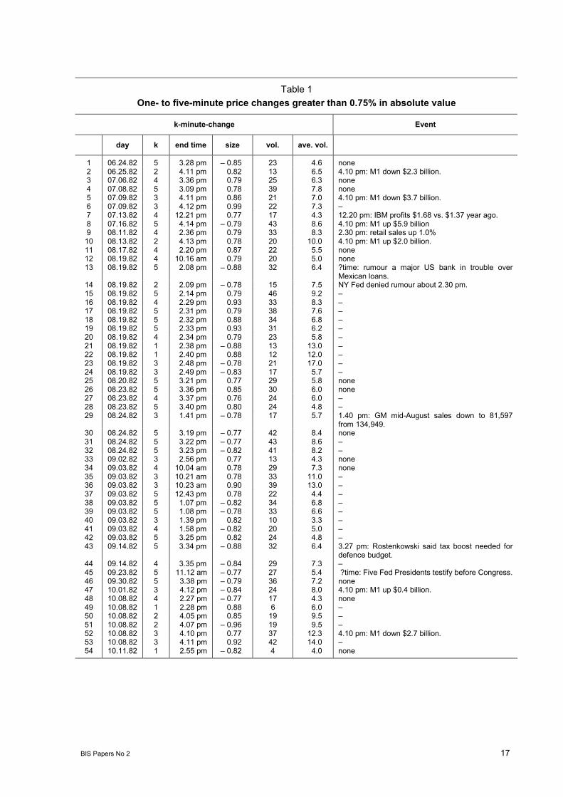
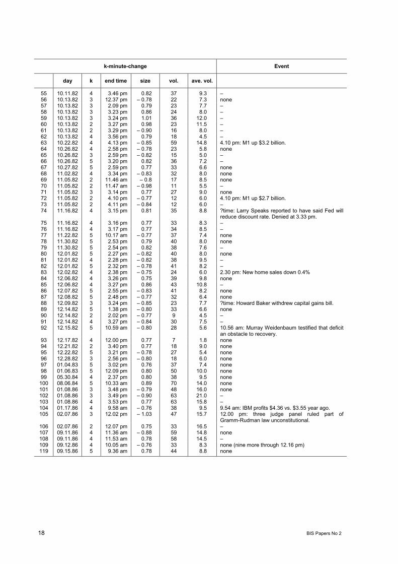
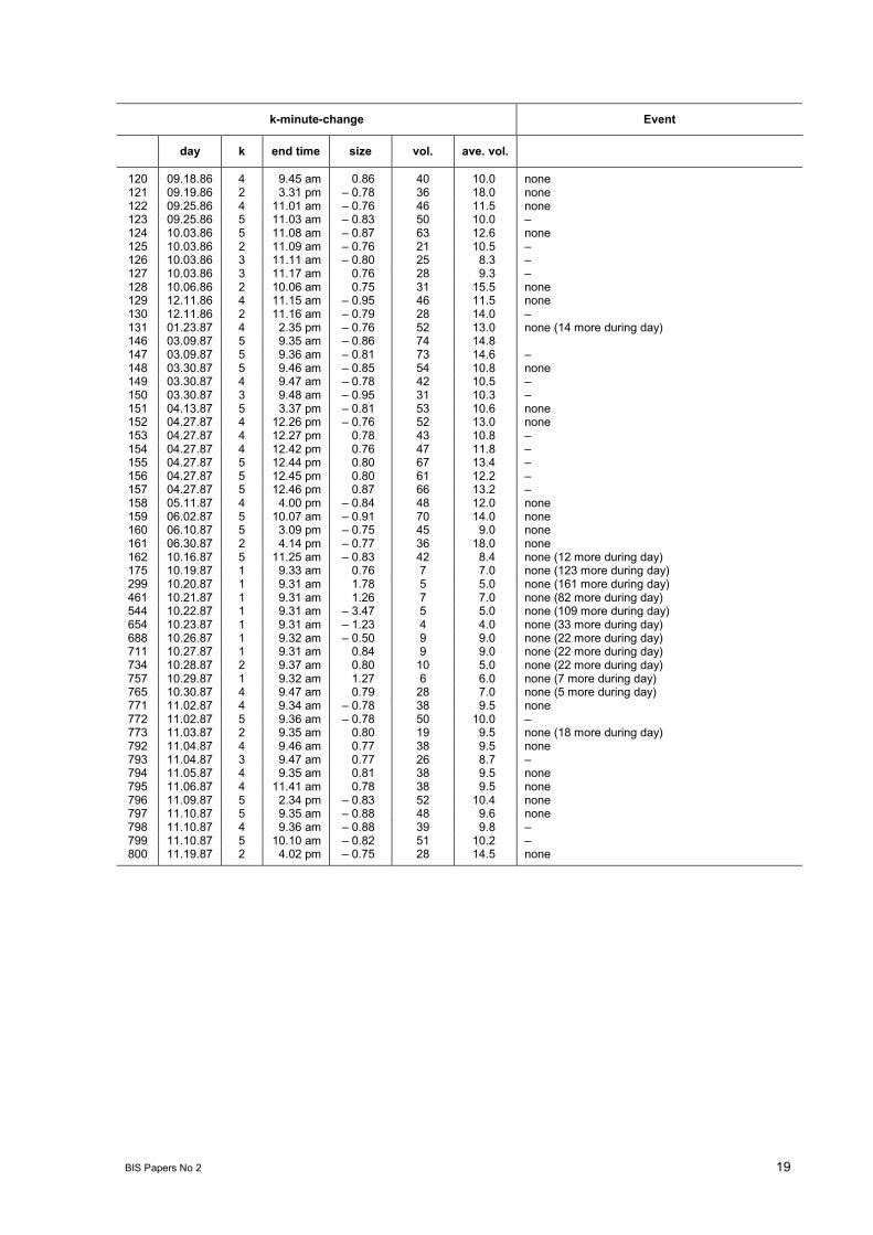
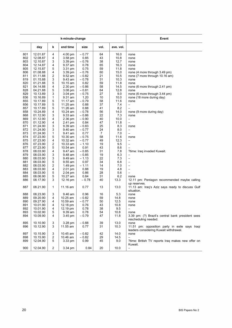
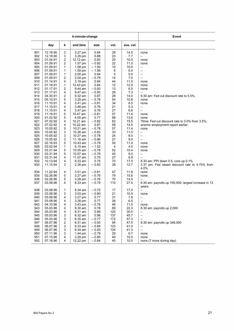
Given each large change, newswires were searched to see if an event could be found that led to thechange. Table 1, which is at the end of this paper, lists the large price changes and the events thatwere found. This paper is essentially a discussion of Table 1. There are 4,417 trading days in thedataset (between 21 April 1982 and 29 October 1999), and in 220 of these days at least one largeprice change occurred, ie a one-to five-minute change greater than or equal to 0.75% in absolutevalue. Events were found for 69 of these days.
Knowledge of the 69 events in Table 1 may prove useful in other studies. Each of these events is bigin that it changed the total value of US equities by a large amount rapidly. This information may beuseful in examining changes in individual stock prices, both absolute and relative to price changes ofother stocks. From a macroeconomic perspective, the events are macro shocks, and knowledge ofthese shocks may be useful in examining various macroeconomic questions.
It is important to stress that this study is purely descriptive. No attempt is made to explain why aparticular event led to the large price change, why other similar events did not lead to large pricechanges, why many large price changes have no events associated with them, and so on. The maincontribution of this paper is simply to list the 69 events.2
1 Cowles Foundation and International Center for Finance, Yale University, New Haven, CT 06520-8281. Voice:203-432 3715; Fax: 203-432-6167; email: [email protected]; website: http://fairmodel.econ.yale.edu. I am indebted toWilliam Nordhaus and Sharon Oster for helpful comments.
2 There does not appear to be other studies in which events have been identified in the way done in this paper. Mitchell andMulherin (1994) and Berry and Howe (1994) examine the effects of the amount of news per unit of time on stock prices andtrading volume. Niederhoffer (1971) examines the effects of the world events on daily stock prices. Boyd, Hu andJagannathan (1999) examine daily S&P 500 changes around days in which there is an employment announcement. Frenchand Roll (1986) examine the volatility of individual stock prices during trading and non-trading hours. Wood, McInsh and Ord(1985) examine the behaviour of a minute-by-minute market return index. Harris (1986) examines the behaviour of portfolioreturns over 15-minute intervals. A number of studies have examined the effects of announcements on daily changes instock prices, and these studies are discussed in Section 4.

10 BIS Papers No 2
It is also important to stress that with a very few exceptions it is almost certain that each of the69 events listed in Table 1 caused the particular price change. The events can thus be interpreted asfacts. For example, it is almost certain that the five-minute price decrease of 0.79% on 16 July 1982was essentially all due to the 4.10 pm money supply announcement (see line 8, Table 1). There wouldlikely have been, of course, a price change had there been no announcement, since the pricegenerally changes each minute, but with a standard deviation of 0.112%, a typical price change is verysmall relative to a change of 0.79%. For all intents and purposes one can attribute all of the pricechange to the money supply announcement.
A way of thinking about the events is the following. Consider asking stock brokers a few minutes afterthe occurrence of one of the price changes in Table 1 that is associated with an event what led, ifanything, to the change. The main point here is that almost without exception the brokers would saythe event. Some events may have been missed - more will be said about this later - but there is littledoubt that each of the 69 events chosen led to the particular price change.
The construction of Table 1 is discussed in Section 2, and the results are discussed in Sections 3and 4.
2. The construction of Table 1The price of an S&P 500 futures contract follows closely the value of the S&P 500 index. Since theS&P 500 index includes most US stocks by market value, the price of an S&P 500 futures contract is agood indicator of the total value of US equities. Tick data are available for the S&P 500 futurescontracts from April 1982 on.3 For Regular Trading Hours (RTH) the tick data per day begin at10.00 am prior to 30 September 1985, and at 9.30 am after that.4 The RTH data end at 4.15pm, whichis 15 minutes after the regular market has closed. Beginning in 1994 the contracts were traded afterhours on the GLOBEX market, and tick data are available for these trades as well. These data beginat 4.30 pm and end at 9.15 am the next day. The GLOBEX market is closed Friday night and all daySaturday. It opens at 6.30 pm Sunday night.
For this study the RTH data begin in 21 April 1982 and end in 29 October 1999. Data are missing forthe last half of December 1991 - the 1991 data end 13 December. The GLOBEX data begin in4 January 1994 and end in 29 October 1999. Data are missing for the last half of 1998 - the 1998GLOBEX data end 31 July. Many government announcements of macroeconomic data occur at8.30 am, and since the GLOBEX market is open at this time, it can respond immediately to theseannouncements. Had the GLOBEX market been in existence back to 1982 and tick data beenavailable, it is likely that many more large price changes and associated events would have beenfound. It is also likely that a number of large price changes and associated events would have beenfound in GLOBEX data for the last half of 1998 had the data been available.
The one-minute price change was taken to be the price of the last trade in the current minute intervalless the price of the last trade in the previous minute interval (all changes in % terms). The two-minuteprice change was taken to be the price of the last trade in the current minute interval less the price ofthe last trade in the minute interval two minutes ago, and so on through five-minute price change.
Table 1 lists the following (a large change is always a change greater than or equal to 0.75% inabsolute value): (1) all large one-minute price changes; (2) all large two-minute price changes exceptwhen at least one of the two one-minute price changes is large; (3) all large three-minute pricechanges except when at least one of the two two-minute price changes is large; (4) all largefour-minute price changes except when at least one of the four one-minute price changes is large or atleast one of the three two-minute price changes is large or at least on of the two three-minute pricechanges is large, and; (5) all large five-minute price changes except when at least one of the fiveone-minute price changes is large or at least one of the four two-minute price changes is large or atleast one of the three three-minute price changes is large or at least one of the two four-minute pricechanges is large. This procedure finds all the large one- through five-minute price changes without
3 The tick data were purchased from the Futures Industry Institute, which obtains the data from the Chicago MercantileExchange.
4 All times in this paper are Eastern even though the RTH and GLOBEX markets are in the Central time zone.

BIS Papers No 2 11
duplication. The most actively traded contract on the particular day was used for these calculations. Ascan be seen from Table 1, there were a total of 1,159 changes chosen.
The end time in Table 1 is the time at the end of the k-minute change, where k ranges from 1 to 5.Vol. is the total number of ticks in the k-minute interval, and ave. vol. is the average number of ticksper minute.
The next step was to see which event, if any, led to the large and rapid change. The Dow JonesInteractive service on the internet was used for this purpose. This service allows one to search fornews reports by time of day. The following four news services were searched: Dow Jones NewsService, Associated Press Newswire, New York Times and Wall Street Journal.
For example, the first case in Table 1 is for 24 June 1982, where at 3.28 pm the price had fallen by0.85% in the last five minutes. For this case the news services were searched for news reportsbetween 3.00 pm and 4.00 pm to see what happened about 3.23 pm that led to the large change. Inthis case no news report was found that seemed likely to have led to change.
In the next case in Table 1 an event was found, which was the 4.10 pm announcement that M1 wasdown $2.3 billion. In the two minutes following the annoucement the price rose 0.82%. Although theregular stock market is closed at 4.00 pm, the RTH market does not close until 4.15 pm, and so theRTH market has time to respond to the money supply announcements.
In some cases an event was found that seemed almost surely to have led to the price change, but forwhich no exact time could be found. In these cases ?time is used in Table 1 to denote that the exacttime of the event was not found. For the 9 October 1990 change it is not completely clear that theBrazil event in fact led to the change, and this is indicated by a (?) in the table. For the1 August 1997 change is unclear which of the three events listed led to the change, and this is alsoindicated by a (?) in the table.
An important government announcement each month is the employment report. This report is releasedat 8.30 am, and it contains data from both the household survey and the establishment survey. Themain variable of interest from the household survey is the unemployment rate, and the main twovariables of interest from the establishment survey are the number of jobs (called payrolls) andaverage hourly earnings. The variable that gets the most attention is the payroll variable, and so thepayroll announcement is listed in Table 1. The event is, however, the entire employment report.
To save space in Table 1, not all large changes following an initial large change are listed for aparticular day, especially on highly volatile days. When some changes are omitted, it is alwaysindicated how many changes are omitted.5
3. Discussion of Table 1Although, as discussed in Section 1, it is almost certain that each of the 69 events listed in Table 1caused the particular price change, it may be that some events have been missed (aside from themissing RTH and GLOBEX data). The most likely error is an event for which there was no newsreport. Less likely is a news report that was listed in the search but that was not noticed as animportant event. The number of events missed is likely to be small, probably fewer than ten.Remember, however, that many more large price changes and events would likely have been foundhad the GLOBEX market been in existence prior to 1994.
Assuming that the number of events that have been missed is small, Table 1 shows that there aremany large price changes that are not due to identifiable events. There are, for example, no eventsassociated with any of the large number of large price changes in October 1987. Regarding the pricechanges with no events, consider the thought experiment about stockbrokers mentioned in Section 1.For the price changes with no associated events in Table 1, what would stockbrokers say a fewminutes after the change? The argument here is that except for the few events that might have beenmissed in the newswire searches, the brokers would not come up with a unique event. Some might
5 A complete table of all the changes is available. This table in pdf format is on the website mentioned in the introductoryfootnote. Click Table 1A near the bottom of the home page of the website for the table.

12 BIS Papers No 2
say there was no event, and some might mention something non-specific like profit taking, renewedconfidence, interest rate fears and the like.
It should be stressed that the events that have been found are not necessarily surprises in the senseof an actual value differing from an expected value, although most of them probably are. Consider, forexample, a payroll announcement. Say that market participants believe that there are three possibleoutcomes regarding the payroll change: 100,000, 300,000 and 500,000 jobs. Assume that marketparticipants weight each possibility equally, so that the expected value is 300,000. Assume also thatthe participants expect that the Fed will leave the funds rate unchanged if the outcome is 100,000 or300,000, but raise the funds rate if the outcome is 500,000. Assume finally that participants expect theS&P 500 price to be 1,430 if there is no funds rate change and 1,400 if there is one. The expectedvalue of the price is thus 1,420, which if the participants are risk neutral will be the price before theannouncement. In this case even if the actual payroll value is equal to the expected value (300,000),the stock price will change (from 1,420 to 1,430). Simply relieving uncertainty may thus change stockprices even if the announced value is equal to the expected value. The events that have been foundare thus not necessarily surprises.
The main results from Table 1 are the following. First, the breakdown of the 69 events is:
Twenty-two events are money supply or interest rate announcements or testimony bymonetary authorities. In 1982 the focus was on money supply announcements, and after thatit was on the federal funds rate;
fourteen events are payroll announcements (employment reports);
eleven events are CPI or PPI or employment cost index announcements;
six events concern other macroeconomic announcements (NAPM, retail sales, durablegoods, new homes);
five events concern Iraq;
four events concern Congressional issues;
three events concern Brazil or Mexico;
one event is fear of Larry Summers.
The 31 non-monetary macroeconomic announcements (payroll, CPI, PPI, employment cost and other)are indirectly related to monetary policy in that these announcements may change peoplesexpectations about future monetary policy. If, for example, there is a large payroll increase, peoplemay think it is more likely that the Fed will tighten in the future because of fear of inflation. If these 31announcements are added to the 22 direct monetary policy events, this gives 53 of the 69 events thatare directly or indirectly related to monetary policy.
Second, the largest response by far was to the cut in the federal funds rate at 3.14 pm on15 October 1998. The first five one-minute price changes following this announcement were 0.89,1.00. 1.00, 1.29 and 1.00%. This is roughly a 5% increase in five minutes. The announcement of thisrate cut was unusual in that it did not follow a normally scheduled FOMC meeting.
Third, the large price changes are not close to being spread evenly across years. Between 1982 and1993, before the introduction of the GLOBEX market, the number of days of large price changes peryear are respectively: 43, 2, 2, 0, 12, 33, 6, 4, 18, 8, 3 and 1. Between 1994 and 1999 the number ofdays are respectively: 5, 0, 12, 26, 22 (GLOBEX data for the last half of 1998 missing) and 23 (throughOctober).
Finally, as noted above, many large price changes have no events associated with them.
4. Implications for other studiesIt seems clear that no simple model of stock price determination can explain the facts in Table 1.There have, for example, been hundreds of important macroeconomic announcements between 1982and 1999, and only a small fraction have led to a large stock price change. An adequate model wouldneed to explain why the particular events in Table 1 led to large price changes, while many otherseemingly similar events did not. There is also the problem from a model building perspective thatthere are many large price changes for which there appear to be no obvious causes.
BIS Papers No 2 13
A number of statistical studies have examined the effects of announcements on daily changes in stockprices (ie the change from the close of one day to the close of the previous day). The daily % changein a stock index is regressed on estimates of the surprise components of announcements, and thecomponents are tested for their statistical significance. The surprise component of an announcementis the difference between the announced value and an estimate of its expected value. The expectedvalue is usually either taken from a survey or to be a prediction from an autoregressive equation.
This literature generally finds that surprise monetary announcements are significant, but little elseseems to matter. Schwert (1981), Pearce and Roley (1985) and Hardouvelis (1987) find surprisemonetary announcements significant, and McQueen and Roley (1993) find inflation surprisessometimes significant after controlling for different stages of the business cycle. Jain (1988) findssurprise monetary and CPI announcements significant. The results in Table 1 suggest that if anythingis to be found significant in explaining stock prices it is likely to be monetary announcements, which iswhat the literature tends to find. The facts in Table 1 thus provide some support to the statisticalresults using daily data, but they also suggest that an adequate model of stock price determination islikely to be more complicated than the models that have been used so far for the statistical tests.
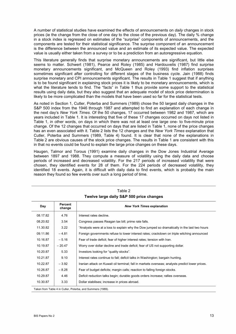
As noted in Section 1, Cutler, Poterba and Summers (1989) chose the 50 largest daily changes in theS&P 500 index from the 1946 through 1987 and attempted to find an explanation of each change inthe next days New York Times. Of the 50 changes, 17 occurred between 1982 and 1987, which areyears included in Table 1. It is interesting that five of these 17 changes occurred on days not listed inTable 1, in other words, on days in which there was not at least one large one- to five-minute pricechange. Of the 12 changes that occurred on days that are listed in Table 1, none of the price changeshas an even associated with it. Table 2 lists the 12 changes and the New York Times explanation thatCutler, Poterba and Summers (1989, Table 4) found. It is clear that none of the explanations inTable 2 are obvious causes of the stock price changes. The results in Table 1 are consistent with thisin that no events could be found to explain the large price changes on these days.
Haugen, Talmor and Torous (1991) examine daily changes in the Dow Jones Industrial Averagebetween 1897 and 1988. They compute a measure of volatility using the daily data and chooseperiods of increased and decreased volatility. For the 217 periods of increased volatility that werechosen, they identified events for 28 of them. For the 224 periods of decreased volatility, theyidentified 18 events. Again, it is difficult with daily data to find events, which is probably the mainreason they found so few events over such a long period of time.
Table 2Twelve large daily S&P 500 price changes
Day Percentchange New York Times explanation
08.17.82 4.76 Interest rates decline.
08.20.82 3.54 Congress passes Reagan tax bill; prime rate falls.
11.30.82 3.22 Analysts were at a loss to explain why the Dow jumped so dramatically in the last two hours
09.11.86 4.81 Foreign governments refuse to lower interest rates; crackdown on triple witching announced
10.16.87 5.16 Fear of trade deficit; fear of higher interest rates; tension with Iran.
10.19.87 20.47 Worry over dollar decline and trade deficit; fear of US not supporting dollar.
10.20.87 5.33 Investors looking for quality stocks.
10.21.87 9.10 Interest rates continue to fall; deficit talks in Washington; bargain hunting.
10.22.87 3.92 Iranian attack on Kuwait oil terminal; fall in markets overseas; analysts predict lower prices.
10.26.87 8.28 Fear of budget deficits; margin calls; reaction to falling foreign stocks.
10.29.87 4.46 Deficit reduction talks begin; durable goods orders increase; rallies overseas.
10.30.87 3.33 Dollar stabilises; increase in prices abroad.
Taken from Table 4 in Cutler, Poterba, and Summers (1989).

14 BIS Papers No 2
Fleming and Remolona (1997) (FR) examine five-minute price changes for the five year US Treasurynote for the period 23 August 1993 - 19 August 1994. They chose the 25 largest five-minute pricechanges over this period, and they find that each of these changes was preceded by amacroeconomic announcement. Of these 25 changes, 17 are on days for which S&P 500 futures dataexist. Data for these 17 days are presented in Table 3. The five-minute bond price change ispresented (taken from Table 3 in Fleming and Remolona (1997)) along with the five-minute S&P 500futures price change.6
The stock price changes in Table 3 are in general fairly large, although not nearly as large as 0.75%,the Table 1 cutoff. It is remarkable that in every case except the last one the bond and stock pricechanges are in the same direction. The direction is the same in the last case if the same time1.45-1.50pm is used, but not if 1.16-1.21 pm is used for the stock price. As FR point out (p32), bondand stock prices need not move in the same direction following an announcement, since stock pricesdepend on expectations of both earnings and interest rates, whereas bond prices depend only onexpectations of interest rates. The fact that they do move in the same direction suggests that theannouncements mostly affect interest rate expectations.
Finally, Gwilym, McMillan and Speight (1999) examine five-minute stock price changes for the UKmarket using FTSE-100 data. The data are for the 24 January 1992 - 30 June 1995 period. Amongother things, their data show that trading volume is higher around announcement times thanotherwise. The results in Table 1 are consistent with this conclusion. For example, note that in generalvolume is quite high around the 8.30 am announcements in the table.
5. ConclusionAs mentioned in the Introduction, this study is purely descriptive. By focusing on very short timeintervals, it has been possible to associate particular events with particular stock price changes,something which is generally not possible to do using daily data. Sixty-nine events have beenidentified between 1982 and 1999 that led to a one- to five-minute S&P 500 futures price changegreater than or equal to 0.75% in absolute value. Knowledge of these events may prove useful in bothmacroeconomic studies and studies of individual stock prices.
The results in Table 1 suggest that stock price determination is complicated. Many large price changescorrespond to no obvious events, and so many large changes appear to have no easy explanation.Also, of the hundreds of fairly similar announcements that have taken place between 1982 and 1999,only a few have led to large price changes (ie those in Table 1), and it does not appear easy to explainwhy some do and some do not.
6 In some cases slightly different time intervals from the FR intervals were used. For the 8.30 am announcements,8.29-8.34 am instead of 8.30-8.35 am was used, since at least in the S&P 500 futures data an 8.30 am announcementaffects the 8.30 am price. For 3 June 1994, 8.30 am employment announcement, FR used 8.40-8.45 am and this was alsodone here. There was very little change in the price before 8.40 am. For the 2.26 pm announcement of the Federal fundsrate on 17 May 1994 FR used 2.35-2.40 pm. In Table 3 both the stock price changes for 2.25-2.30 and 2.35-2.40 pm arepresented. Finally, for the 1.17 pm announcement of the Federal funds rate on 16 August 1994, FR used 1.45-1.50 pm, andin Table 3 both the stock price changes for 1.16-1:21 pm and 1.45-1.50 pm are presented.

BIS Papers No 2 15
Table 3Five-minute bond and stock price changes
Day Bondinterval
Bondchange
Stockinterval
Stockchange Announcement
01.07.94 8.30-8.35 am 0.282 8.28-8.33 am 0.07 8.30 am: Employment
02.04.94 8.30-8.35 am 0.315 8.29-8.34 am 0.15 8.30 am: Employment
02.04.94 11.05-11.10 am 0.259 11.04-11.09 am 0.09 11.05 am: Federal funds rate
02.11.94 8.30-8.35 am 0.223 8.29-8.34 am 0.31 8.30 am: PPI, retail sales
04.13.94 8.30-8.35 am 0.224 8.29-8.34 am 0.10 8.30 am: CPI, retail sales
05.06.94 8.30-8.35 am 0.536 8.28-8.33 am 0.14 8.30 am: Employment
05.11.94 1.40-1.45 pm 0.223 1.40-1.45 pm 0.37 1.42 pm: 10-year-note auctionresults
05.12.94 8.30-8.35 am 0.384 8.29-8.34 am 0.43 8.30 am: PPI, retail sales
05.17.94 2.35-2.40 pm 0.221 2.25-2.30 pm 0.33 2.26 pm: Federal funds rate
2.35-2.40 pm 0.00
05.27.94 8.30-8.35 am 0.343 8.29-8.34 am 0.20 8.30 am: GDP
06.03.94 8.40-8.45 am 0.265 8.40-8.45 am 0.23 8.30 am: Employment
07.08.94 8.30-8.35 am 0.440 8.29-8.34 am 0.30 8.30 am: Employment
07.12.94 8.30-8.35 am 0.222 8.29-8.34 am 0.28 8.30 am: PPI
07.14.94 8.30-8.35 am 0.253 8.29-8.34 am 0.11 8.30 am: Retail sales
07.29.94 8.30-8.35 am 0.407 8.29-8.34 am 0.31 8.30 am: GDP
08.05.94 8.30-8.35 am 0.590 8.29-8.34 am 0.35 8.30 am: Employment
08.16.94 1.45-1.50 pm 0.266 1.16-1.21 pm 0.23 1.17 pm: Federal funds rate
1.45-1.50pm 0.09
Notes: No stock trades at 8.29 am on 1.07.94 and 5.06.94. Changes are percent changes. Bond results and announcement information takenfrom Table 3 in Fleming and Remolona (1997).

16 BIS Papers No 2
ReferencesBerry, Thomas D and Keith M Howe, 1994, Public Information Arrival, Journal of Finance, 49,1331-1346.
Boyd, John H, Jian Hu and Ravi Jagannathan, 1999, The Stock Markets Reaction to UnemploymentNews: Why Bad News May Sometimes Be Good For Stocks ?, Working paper, 12 November.
Cutler, David M, James M Poterba and Lawrence H Summers, 1989, What Moves Stock Prices?,Journal of Portfolio Management, 15, 4-12.
Fleming, Michael J and Eli M Remolona, 1997, What Moves the Bond Market?, FRBNY EconomicPolicy Review, December.
French, Kenneth R and Richard Roll, 1986, Stock Return Variances: The Arrival of Information andthe Reaction of Traders, Journal of Financial Economics, 17, 5-26.
Gwilym, Owain A P, David McMillan and Alan Speight, The Intraday Relationship between Volumeand Volatility in LIFFE Futures Markets, Applied Financial Economics, 9, 593-604.
Hardouvelis, Gikas A, 1987, Macroeconomic Information and Stock Prices, Journal of Economicsand Business, 39, 131-140.
Harris, Lawrence, 1986, A Transaction Data Study of Weekly and Intradaily Patterns in StockReturns, Journal of Financial Economics, 16, 99-117.
Haugen, Robert A, Eli Talmor and Walter N Torous, 1991, The Effect of Volatility Changes on theLevel of Stock Prices and Subsequent Expected Returns, Journal of Finance, 46, 985-1007.
Jain, Prem C, 1988, Response of Hourly Stock Prices and Trading Volume to Economic News,Journal of Business, 61, 219-231.
McQueen, Grant, and V Vance Roley, 1993, Stock Prices, News, and Business Conditions, Reviewof Financial Studies, 6, 683-707.
Mitchell, Mark L and J Harold Mulherin, 1994, The Impact of Public Information on the Stock Market,Journal of Finance, 49, 923-950.
Niederhoffer, Victor, 1971, The Analysis of World Events and Stock Prices, Journal of Business, 44,193-219.
Pearce, Douglas K and V Vance Rolex, 1985, Stock Prices and Economic News,Journalof Business, 58, 49-67.
Schwert, G William, 1981, The Adjustment of Stock Prices to Information about Inflation, Journal ofFinance, 56, 15-29.
Wood, Robert A, Thomas H McInsh and J Keith Ord, 1985, An Investigation of Transactions Data forNYSE Stocks, Journal of Finance, 40, 723-739.
BIS Papers No 2 17
Table 1One- to five-minute price changes greater than 0.75% in absolute value
k-minute-change Event
day k end time size vol. ave. vol.
1 06.24.82 5 3.28 pm 0.85 23 4.6 none2 06.25.82 2 4.11 pm 0.82 13 6.5 4.10 pm: M1 down $2.3 billion.3 07.06.82 4 3.36 pm 0.79 25 6.3 none4 07.08.82 5 3.09 pm 0.78 39 7.8 none5 07.09.82 3 4.11 pm 0.86 21 7.0 4.10 pm: M1 down $3.7 billion.6 07.09.82 3 4.12 pm 0.99 22 7.3 7 07.13.82 4 12.21 pm 0.77 17 4.3 12.20 pm: IBM profits $1.68 vs. $1.37 year ago.8 07.16.82 5 4.14 pm 0.79 43 8.6 4.10 pm: M1 up $5.9 billion9 08.11.82 4 2.36 pm 0.79 33 8.3 2.30 pm: retail sales up 1.0%10 08.13.82 2 4.13 pm 0.78 20 10.0 4.10 pm: M1 up $2.0 billion.11 08.17.82 4 2.20 pm 0.87 22 5.5 none12 08.19.82 4 10.16 am 0.79 20 5.0 none13 08.19.82 5 2.08 pm 0.88 32 6.4 ?time: rumour a major US bank in trouble over
Mexican loans.14 08.19.82 2 2.09 pm 0.78 15 7.5 NY Fed denied rumour about 2.30 pm.15 08.19.82 5 2.14 pm 0.79 46 9.2 16 08.19.82 4 2.29 pm 0.93 33 8.3 17 08.19.82 5 2.31 pm 0.79 38 7.6 18 08.19.82 5 2.32 pm 0.88 34 6.8 19 08.19.82 5 2.33 pm 0.93 31 6.2 20 08.19.82 4 2.34 pm 0.79 23 5.8 21 08.19.82 1 2.38 pm 0.88 13 13.0 22 08.19.82 1 2.40 pm 0.88 12 12.0 23 08.19.82 3 2.48 pm 0.78 21 17.0 24 08.19.82 3 2.49 pm 0.83 17 5.7 25 08.20.82 5 3.21 pm 0.77 29 5.8 none26 08.23.82 5 3.36 pm 0.85 30 6.0 none27 08.23.82 4 3.37 pm 0.76 24 6.0 28 08.23.82 5 3.40 pm 0.80 24 4.8 29 08.24.82 3 1.41 pm 0.78 17 5.7 1.40 pm: GM mid-August sales down to 81,597
from 134,949.30 08.24.82 5 3.19 pm 0.77 42 8.4 none31 08.24.82 5 3.22 pm 0.77 43 8.6 32 08.24.82 5 3.23 pm 0.82 41 8.2 33 09.02.82 3 2.56 pm 0.77 13 4.3 none34 09.03.82 4 10.04 am 0.78 29 7.3 none35 09.03.82 3 10.21 am 0.78 33 11.0 36 09.03.82 3 10.23 am 0.90 39 13.0 37 09.03.82 5 12.43 pm 0.78 22 4.4 38 09.03.82 5 1.07 pm 0.82 34 6.8 39 09.03.82 5 1.08 pm 0.78 33 6.6 40 09.03.82 3 1.39 pm 0.82 10 3.3 41 09.03.82 4 1.58 pm 0.82 20 5.0 42 09.03.82 5 3.25 pm 0.82 24 4.8 43 09.14.82 5 3.34 pm 0.88 32 6.4 3.27 pm: Rostenkowski said tax boost needed for
defence budget.44 09.14.82 4 3.35 pm 0.84 29 7.3 45 09.23.82 5 11.12 am 0.77 27 5.4 ?time: Five Fed Presidents testify before Congress.46 09.30.82 5 3.38 pm 0.79 36 7.2 none47 10.01.82 3 4.12 pm 0.84 24 8.0 4.10 pm: M1 up $0.4 billion.48 10.08.82 4 2.27 pm 0.77 17 4.3 none49 10.08.82 1 2.28 pm 0.88 6 6.0 50 10.08.82 2 4.05 pm 0.85 19 9.5 51 10.08.82 2 4.07 pm 0.96 19 9.5 52 10.08.82 3 4.10 pm 0.77 37 12.3 4.10 pm: M1 down $2.7 billion.53 10.08.82 3 4.11 pm 0.92 42 14.0 54 10.11.82 1 2.55 pm 0.82 4 4.0 none
18 BIS Papers No 2
k-minute-change Event
day k end time size vol. ave. vol.
55 10.11.82 4 3.46 pm 0.82 37 9.3 56 10.13.82 3 12.37 pm 0.78 22 7.3 none57 10.13.82 3 2.09 pm 0.79 23 7.7 58 10.13.82 3 3.23 pm 0.86 24 8.0 59 10.13.82 3 3.24 pm 1.01 36 12.0 60 10.13.82 2 3.27 pm 0.98 23 11.5 61 10.13.82 2 3.29 pm 0.90 16 8.0 62 10.13.82 4 3.56 pm 0.79 18 4.5 63 10.22.82 4 4.13 pm 0.85 59 14.8 4.10 pm: M1 up $3.2 billion.64 10.26.82 4 2.58 pm 0.78 23 5.8 none65 10.26.82 3 2.59 pm 0.82 15 5.0 66 10.26.82 5 3.20 pm 0.82 36 7.2 67 10.27.82 5 2.59 pm 0.77 33 6.6 none68 11.02.82 4 3.34 pm 0.83 32 8.0 none69 11.05.82 2 11.46 am 0.8 17 8.5 none70 11.05.82 2 11.47 am 0.98 11 5.5 71 11.05.82 3 3.14 pm 0.77 27 9.0 none72 11.05.82 2 4.10 pm 0.77 12 6.0 4.10 pm: M1 up $2.7 billion.73 11.05.82 2 4.11 pm 0.84 12 6.0 74 11.16.82 4 3.15 pm 0.81 35 8.8 ?time: Larry Speaks reported to have said Fed will
reduce discount rate. Denied at 3.33 pm.75 11.16.82 4 3.16 pm 0.77 33 8.3 76 11.16.82 4 3.17 pm 0.77 34 8.5 77 11.22.82 5 10.17 am 0.77 37 7.4 none78 11.30.82 5 2.53 pm 0.79 40 8.0 none79 11.30.82 5 2.54 pm 0.82 38 7.6 80 12.01.82 5 2.27 pm 0.82 40 8.0 none81 12.01.82 4 2.28 pm 0.82 38 9.5 82 12.01.82 5 2.32 pm 0.78 41 8.2 83 12.02.82 4 2.38 pm 0.75 24 6.0 2.30 pm: New home sales down 0.4%84 12.06.82 4 3.26 pm 0.75 39 9.8 none85 12.06.82 4 3.27 pm 0.86 43 10.8 86 12.07.82 5 2.55 pm 0.83 41 8.2 none87 12.08.82 5 2.48 pm 0.77 32 6.4 none88 12.09.82 3 3.24 pm 0.85 23 7.7 ?time: Howard Baker withdrew capital gains bill.89 12.14.82 5 1.38 pm 0.80 33 6.6 none90 12.14.82 2 2.02 pm 0.77 9 4.5 91 12.14.82 4 3.27 pm 0.84 30 7.5 92 12.15.82 5 10.59 am 0.80 28 5.6 10.56 am: Murray Weidenbaum testified that deficit
an obstacle to recovery.93 12.17.82 4 12.00 pm 0.77 7 1.8 none94 12.21.82 2 3.40 pm 0.77 18 9.0 none95 12.22.82 5 3.21 pm 0.78 27 5.4 none96 12.28.82 3 2.56 pm 0.80 18 6.0 none97 01.04.83 5 3.02 pm 0.76 37 7.4 none98 01.06.83 5 12.09 pm 0.80 50 10.0 none99 05.30.84 4 2.37 pm 0.80 38 9.5 none
100 08.06.84 5 10.33 am 0.89 70 14.0 none101 01.08.86 3 3.48 pm 0.79 48 16.0 none102 01.08.86 3 3.49 pm 0.90 63 21.0 103 01.08.86 4 3.53 pm 0.77 63 15.8 104 01.17.86 4 9.58 am 0.76 38 9.5 9.54 am: IBM profits $4.36 vs. $3.55 year ago.105 02.07.86 3 12.02 pm 1.03 47 15.7 12.00 pm: three judge panel ruled part of
Gramm-Rudman law unconstitutional.106 02.07.86 2 12.07 pm 0.75 33 16.5 107 09.11.86 4 11.36 am 0.88 59 14.8 none108 09.11.86 4 11.53 am 0.78 58 14.5 109 09.12.86 4 10.05 am 0.76 33 8.3 none (nine more through 12.16 pm)119 09.15.86 5 9.36 am 0.78 44 8.8 none
BIS Papers No 2 19
k-minute-change Event
day k end time size vol. ave. vol.
120 09.18.86 4 9.45 am 0.86 40 10.0 none121 09.19.86 2 3.31 pm 0.78 36 18.0 none122 09.25.86 4 11.01 am 0.76 46 11.5 none123 09.25.86 5 11.03 am 0.83 50 10.0 124 10.03.86 5 11.08 am 0.87 63 12.6 none125 10.03.86 2 11.09 am 0.76 21 10.5 126 10.03.86 3 11.11 am 0.80 25 8.3 127 10.03.86 3 11.17 am 0.76 28 9.3 128 10.06.86 2 10.06 am 0.75 31 15.5 none129 12.11.86 4 11.15 am 0.95 46 11.5 none130 12.11.86 2 11.16 am 0.79 28 14.0 131 01.23.87 4 2.35 pm 0.76 52 13.0 none (14 more during day)146 03.09.87 5 9.35 am 0.86 74 14.8147 03.09.87 5 9.36 am 0.81 73 14.6 148 03.30.87 5 9.46 am 0.85 54 10.8 none149 03.30.87 4 9.47 am 0.78 42 10.5 150 03.30.87 3 9.48 am 0.95 31 10.3 151 04.13.87 5 3.37 pm 0.81 53 10.6 none152 04.27.87 4 12.26 pm 0.76 52 13.0 none153 04.27.87 4 12.27 pm 0.78 43 10.8 154 04.27.87 4 12.42 pm 0.76 47 11.8 155 04.27.87 5 12.44 pm 0.80 67 13.4 156 04.27.87 5 12.45 pm 0.80 61 12.2 157 04.27.87 5 12.46 pm 0.87 66 13.2 158 05.11.87 4 4.00 pm 0.84 48 12.0 none159 06.02.87 5 10.07 am 0.91 70 14.0 none160 06.10.87 5 3.09 pm 0.75 45 9.0 none161 06.30.87 2 4.14 pm 0.77 36 18.0 none162 10.16.87 5 11.25 am 0.83 42 8.4 none (12 more during day)175 10.19.87 1 9.33 am 0.76 7 7.0 none (123 more during day)299 10.20.87 1 9.31 am 1.78 5 5.0 none (161 more during day)461 10.21.87 1 9.31 am 1.26 7 7.0 none (82 more during day)544 10.22.87 1 9.31 am 3.47 5 5.0 none (109 more during day)654 10.23.87 1 9.31 am 1.23 4 4.0 none (33 more during day)688 10.26.87 1 9.32 am 0.50 9 9.0 none (22 more during day)711 10.27.87 1 9.31 am 0.84 9 9.0 none (22 more during day)734 10.28.87 2 9.37 am 0.80 10 5.0 none (22 more during day)757 10.29.87 1 9.32 am 1.27 6 6.0 none (7 more during day)765 10.30.87 4 9.47 am 0.79 28 7.0 none (5 more during day)771 11.02.87 4 9.34 am 0.78 38 9.5 none772 11.02.87 5 9.36 am 0.78 50 10.0 773 11.03.87 2 9.35 am 0.80 19 9.5 none (18 more during day)792 11.04.87 4 9.46 am 0.77 38 9.5 none793 11.04.87 3 9.47 am 0.77 26 8.7 794 11.05.87 4 9.35 am 0.81 38 9.5 none795 11.06.87 4 11.41 am 0.78 38 9.5 none796 11.09.87 5 2.34 pm 0.83 52 10.4 none797 11.10.87 5 9.35 am 0.88 48 9.6 none798 11.10.87 4 9.36 am 0.88 39 9.8 799 11.10.87 5 10.10 am 0.82 51 10.2 800 11.19.87 2 4.02 pm 0.75 28 14.5 none
20 BIS Papers No 2
k-minute-change Event
day k end time size vol. ave. vol.
801 12.01.87 4 4.00 pm 0.77 64 16.0 none802 12.08.87 4 3.58 pm 0.85 43 10.8 none803 12.10.87 3 3.39 pm 0.76 38 12.7 none804 12.14.87 4 9.37 am 0.78 65 16.3 none805 12.15.87 5 3.31 pm 0.75 59 11.8 none806 01.08.88 4 3.39 pm 0.76 60 15.0 none (4 more through 3.49 pm)811 01.11.88 2 9.52 am 0.82 21 10.5 none (7 more through 10.16 am)819 01.15.88 3 9.43 am 0.78 31 10.3 none820 01.21.88 5 10.15 am 0.82 59 11.8 none821 04.14.88 4 2.30 pm 0.86 58 14.5 none (6 more through 2.41 pm)828 04.21.88 5 3.08 pm 0.81 64 12.8 none829 10.13.89 3 3.04 pm 0.75 27 9.0 none (6 more through 3.44 pm)836 10.16.89 1 9.31 am 1.20 10 10.0 none (18 more during day)855 10.17.89 5 11.17 am 0.79 58 11.6 none856 10.17.89 5 11.25 am 0.88 37 7.4 857 10.17.89 5 11.26 am 0.88 41 8.2 858 10.24.89 4 10.24 am 0.78 56 14.0 none (9 more during day)868 01.12.90 3 9.33 am 0.86 22 7.3 none869 01.12.90 4 2.36 pm 0.90 40 10.0 870 01.12.90 4 2.41 pm 0.84 47 11.8 871 01.24.90 3 9.39 am 0.83 25 8.3 none872 01.24.90 3 9.40 am 0.77 24 8.0 873 01.24.90 1 9.41 am 0.77 7 7.0 874 07.23.90 5 10.30 am 0.75 58 11.6 none875 07.23.90 4 10.32 am 0.77 49 12.3 876 07.23.90 2 10.33 am 1.10 19 9.5 877 07.23.90 5 10.54 am 0.91 43 8.6 878 08.03.90 4 9.47 am 0.85 31 7.8 ?time: Iraq invaded Kuwait.879 08.03.90 3 9.48 am 0.85 19 6.3 880 08.03.90 3 9.49 am 1.13 22 7.3 881 08.03.90 5 9.55 am 0.97 34 6.8 882 08.03.90 2 1.49 pm 1.11 14 7.0 883 08.03.90 4 2.01 pm 0.88 19 4.8 884 08.03.90 5 2.04 pm 0.86 28 5.6 885 08.06.90 5 10.27 am 0.84 31 6.2 none886 08.17.90 3 12.16 pm 0.78 40 13.3 12.11 pm: Pentagon recommended maybe calling
up reserves.887 08.21.90 1 11.16 am 0.77 13 13.0 11.13 am: Iraqs Aziz says ready to discuss Gulf
situation.888 08.23.90 3 9.46 am 0.96 16 5.3 none889 09.20.90 4 10.25 am 0.82 59 14.8 none890 09.27.90 4 10.59 am 0.77 50 12.5 none891 10.01.90 4 12.18 pm 0.76 43 10.8 none892 10.01.90 4 12.19 pm 0.78 38 9.5 893 10.02.90 5 9.39 am 0.78 54 10.8 none894 10.09.90 4 3.45 pm 0.79 47 11.8 3.39 pm: (?) Brazils central bank president sees
rescheduling needed.895 10.10.90 3 3.28 pm 0.88 39 13.0 none896 10.12.90 3 11.55 am 0.77 31 10.3 11.51 pm: opposition party in exile says Iraqi
leaders considering Kuwait withdrawal.897 10.15.90 3 10.45 am 0.82 42 14.0 none898 10.15.90 2 10.46 am 0.82 29 14.5 899 12.04.90 5 3.33 pm 0.99 45 9.0 ?time: British TV reports Iraq makes new offer on
Kuwait.900 12.04.90 2 3.34 pm 0.84 20 10.0
BIS Papers No 2 21
k-minute-change Event
day k end time size vol. ave. vol.
901 12.18.90 2 3.27 pm 0.84 29 14.5 none902 12.18.90 3 3.29 pm 0.88 23 7.7 903 01.04.91 2 12.12 pm 0.83 20 10.0 none904 01.09.91 2 1.57 pm 0.92 22 11.0 none905 01.09.91 1 1.58 pm 1.50 10 10.0 906 01.09.91 1 1.59 pm 1.56 6 6.0 907 01.09.91 1 2.00 pm 0.94 5 5.0 909 01.09.91 2 2.04 pm 0.78 14 7.0 910 01.14.91 4 3.19 pm 0.84 44 11.0 none911 01.16.91 1 12.43 pm 0.84 12 12.0 none912 01.17.91 2 9.44 am 0.93 13 6.5 none913 01.17.91 4 9.47 am 0.93 29 7.3 914 04.30.91 2 9.32 am 0.87 28 14.0 9.30 am: Fed cut discount rate to 5.5%.915 05.10.91 5 3.25 pm 0.78 54 10.8 none916 11.15.91 4 3.41 pm 0.81 34 8.5 none917 11.15.91 4 3.46 pm 0.76 21 5.3 918 11.15.91 4 3.47 pm 0.76 27 6.8 919 11.19.91 5 10.47 am 0.81 57 11.4 none920 01.02.92 5 4.05 pm 0.77 68 13.6 none921 07.02.92 4 10.21 am 0.82 62 15.5 ?time: Fed cut discount rate to 3.0% from 3.5%;922 07.02.92 4 10.22 am 0.87 58 14.5 anemic employment report earlier.923 10.05.92 5 10.21 am 0.78 57 11.4 none924 10.05.92 3 10.26 am 0.83 33 11.0 925 10.05.92 3 10.27 am 0.78 24 8.0 926 10.05.92 3 11.16 am 0.86 27 9.0 927 02.16.93 5 10.43 am 0.79 55 11.0 none928 03.02.94 1 5.15 am 1.52 4 4.0 none929 03.31.94 5 10.55 am 0.78 52 10.4 none930 03.31.94 5 10.57 am 0.76 45 9.0 931 03.31.94 4 11.07 am 0.75 27 6.8 932 10.13.94 4 8.33 am 0.75 70 17.5 8.30 am: PPI down 0.5; core up 0.1%933 11.15.94 3 2.38 pm 0.83 38 12.7 2.37 pm: Fed raised discount rate to 4.75% from
4.0%934 11.22.94 4 3.51 pm 0.81 47 11.8 none935 02.26.96 5 3.27 pm 0.76 79 15.8 none936 02.26.96 5 3.28 pm 0.76 70 14.0 937 03.08.96 4 8.33 am 0.79 110 27.5 8.30 am: payrolls up 705,000; largest increase in 12
years.938 03.08.96 1 8.34 am 0.75 17 17.0 939 03.08.96 2 3.03 pm 0.80 21 10.5 none940 03.08.96 4 3.27 pm 0.77 31 7.8 941 03.08.96 4 3.28 pm 0.77 26 6.5 942 04.10.96 4 3.43 pm 0.76 46 11.5 none943 05.03.96 4 8.30 am 0.78 89 22.3 8.30 am: payrolls up 2,000944 05.03.96 4 8.31 am 0.89 120 30.0 945 05.03.96 3 8.32 am 0.96 137 45.7 946 05.03.96 3 8.35 am 0.77 172 57.3 947 06.07.96 2 8.31 am 0.93 94 47.0 8.30 am: payrolls up 348,000948 06.07.96 3 8.33 am 0.84 123 41.0 949 06.07.96 3 8.34 am 0.93 124 41.3 950 07.11.96 3 1.44 pm 0.79 20 6.7 none951 07.15.96 4 3.29 pm 0.85 40 10.0 none952 07.16.96 4 12.22 pm 0.84 40 10.0 none (7 more during day).
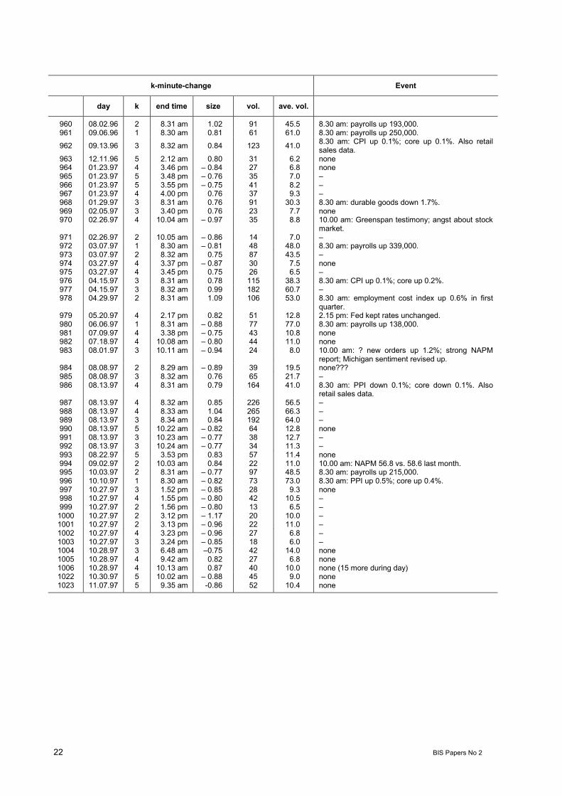
22 BIS Papers No 2
k-minute-change Event
day k end time size vol. ave. vol.
960 08.02.96 2 8.31 am 1.02 91 45.5 8.30 am: payrolls up 193,000.961 09.06.96 1 8.30 am 0.81 61 61.0 8.30 am: payrolls up 250,000.962 09.13.96 3 8.32 am 0.84 123 41.0 8.30 am: CPI up 0.1%; core up 0.1%. Also retail
sales data.963 12.11.96 5 2.12 am 0.80 31 6.2 none964 01.23.97 4 3.46 pm 0.84 27 6.8 none965 01.23.97 5 3.48 pm 0.76 35 7.0 966 01.23.97 5 3.55 pm 0.75 41 8.2 967 01.23.97 4 4.00 pm 0.76 37 9.3 968 01.29.97 3 8.31 am 0.76 91 30.3 8.30 am: durable goods down 1.7%.969 02.05.97 3 3.40 pm 0.76 23 7.7 none970 02.26.97 4 10.04 am 0.97 35 8.8 10.00 am: Greenspan testimony; angst about stock
market.971 02.26.97 2 10.05 am 0.86 14 7.0 972 03.07.97 1 8.30 am 0.81 48 48.0 8.30 am: payrolls up 339,000.973 03.07.97 2 8.32 am 0.75 87 43.5 974 03.27.97 4 3.37 pm 0.87 30 7.5 none975 03.27.97 4 3.45 pm 0.75 26 6.5 976 04.15.97 3 8.31 am 0.78 115 38.3 8.30 am: CPI up 0.1%; core up 0.2%.977 04.15.97 3 8.32 am 0.99 182 60.7 978 04.29.97 2 8.31 am 1.09 106 53.0 8.30 am: employment cost index up 0.6% in first
quarter.979 05.20.97 4 2.17 pm 0.82 51 12.8 2.15 pm: Fed kept rates unchanged.980 06.06.97 1 8.31 am 0.88 77 77.0 8.30 am: payrolls up 138,000.981 07.09.97 4 3.38 pm 0.75 43 10.8 none982 07.18.97 4 10.08 am 0.80 44 11.0 none983 08.01.97 3 10.11 am 0.94 24 8.0 10.00 am: ? new orders up 1.2%; strong NAPM
report; Michigan sentiment revised up.984 08.08.97 2 8.29 am 0.89 39 19.5 none???985 08.08.97 3 8.32 am 0.76 65 21.7 986 08.13.97 4 8.31 am 0.79 164 41.0 8.30 am: PPI down 0.1%; core down 0.1%. Also
retail sales data.987 08.13.97 4 8.32 am 0.85 226 56.5 988 08.13.97 4 8.33 am 1.04 265 66.3 989 08.13.97 3 8.34 am 0.84 192 64.0 990 08.13.97 5 10.22 am 0.82 64 12.8 none991 08.13.97 3 10.23 am 0.77 38 12.7 992 08.13.97 3 10.24 am 0.77 34 11.3 993 08.22.97 5 3.53 pm 0.83 57 11.4 none994 09.02.97 2 10.03 am 0.84 22 11.0 10.00 am: NAPM 56.8 vs. 58.6 last month.995 10.03.97 2 8.31 am 0.77 97 48.5 8.30 am: payrolls up 215,000.996 10.10.97 1 8.30 am 0.82 73 73.0 8.30 am: PPI up 0.5%; core up 0.4%.997 10.27.97 3 1.52 pm 0.85 28 9.3 none998 10.27.97 4 1.55 pm 0.80 42 10.5 999 10.27.97 2 1.56 pm 0.80 13 6.5
1000 10.27.97 2 3.12 pm 1.17 20 10.0 1001 10.27.97 2 3.13 pm 0.96 22 11.0 1002 10.27.97 4 3.23 pm 0.96 27 6.8 1003 10.27.97 3 3.24 pm 0.85 18 6.0 1004 10.28.97 3 6.48 am 0.75 42 14.0 none1005 10.28.97 4 9.42 am 0.82 27 6.8 none1006 10.28.97 4 10.13 am 0.87 40 10.0 none (15 more during day)1022 10.30.97 5 10.02 am 0.88 45 9.0 none1023 11.07.97 5 9.35 am -0.86 52 10.4 none
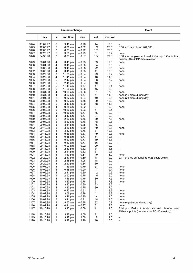
BIS Papers No 2 23
k-minute-change Event
day k end time size vol. ave. vol.
1024 11.07.97 5 9.40 am 0.76 44 8.8 1025 12.05.97 5 8.30 am 0.82 129 25.8 8.30 am: payrolls up 404,000.1026 12.05.97 2 8.31 am 0.92 151 75.5 1027 12.23.97 5 3.56 pm 0.79 51 10.2 none1028 04.30.98 2 8.31 am 0.87 154 77.0 8.30 am: employment cost index up 0.7% in first
quarter. Also GDP data released.1029 08.04.98 4 3.43 pm 0.93 39 9.8 none1030 08.04.98 4 3.46 pm 0.80 34 8.5 1031 08.05.98 4 9.43 am 0.88 22 5.5 none1032 08.05.98 4 3.45 pm 0.93 41 10.3 none1033 08.27.98 3 11.38 am 0.84 29 9.7 none1034 08.27.98 4 11.41 am 0.84 46 11.5 1035 08.27.98 5 2.47 pm 0.84 36 7.2 none1036 08.27.98 5 2.48 pm 0.84 40 8.0 1037 08.28.98 5 11.49 am 0.77 47 9.4 none1038 08.28.98 5 11.50 am 0.86 45 9.0 1039 08.31.98 4 10.09 am 0.96 31 7.8 none1040 08.31.98 4 3.07 pm 0.77 47 11.8 none (10 more during day)1051 09.01.98 2 9.32 am 0.94 19 9.5 none (21 more during day)1073 09.02.98 3 9.37 am 0.75 30 10.0 none1074 09.02.98 5 3.49 pm 0.80 58 11.61075 09.03.98 4 9.35 am 0.82 37 9.3 none1076 09.03.98 5 10.30 am 0.93 47 9.4 1077 09.03.98 5 10.56 am 0.77 45 9.0 1078 09.03.98 4 3.42 pm 0.77 37 9.3 1079 09.04.98 5 2.50 pm 0.76 39 7.8 none1080 09.04.98 5 3.39 pm 0.76 48 9.6 1081 09.04.98 5 3.41 pm 0.85 45 9.0 1082 09.10.98 5 3.36 pm 0.80 49 9.8 none1083 09.10.98 3 3.42 pm 0.76 37 12.3 1084 09.11.98 4 9.46 am 0.87 49 12.3 none1085 09.11.98 4 9.48 am 0.77 51 12.8 1086 09.11.98 5 9.50 am 0.77 69 13.8 1087 09.11.98 3 9.53 am 0.77 36 12.0 1088 09.11.98 2 10.03 am 0.92 20 10.0 1089 09.11.98 4 2.50 pm 0.82 34 8.5 1090 09.11.98 4 2.51 pm 0.82 37 9.3 1091 09.16.98 5 3.43 pm 0.81 40 8.0 none1092 09.29.98 2 2.17 pm 0.89 18 9.0 2.17 pm: fed cut funds rate 25 basis points.1093 09.29.98 2 2.18 pm 1.08 18 9.0 1094 09.29.98 3 2.20 pm 0.84 30 10.0 1095 10.01.98 5 11.19 am 0.79 51 10.2 none1096 10.02.98 5 10.18 am 0.90 47 9.4 none1097 10.02.98 4 12.41 pm 0.80 42 10.5 none1098 10.02.98 5 2.52 pm 0.75 45 9.0 none1099 10.02.98 4 3.15 pm 0.75 30 7.5 none1100 10.05.98 4 3.37 pm 0.78 31 7.8 none1101 10.05.98 4 3.42 pm 0.80 33 8.3 1102 10.05.98 4 3.43 pm 0.75 30 7.5 1103 10.07.98 5 10.12 am 0.91 41 8.2 none1104 10.07.98 5 3.06 pm 0.76 41 8.2 none1105 10.07.98 4 3.26 pm 0.75 44 11.0 none1106 10.07.98 5 3.41 pm 0.91 48 9.6 none1107 10.08.98 3 9.50 am 0.78 32 10.7 none (eight more during day)1116 10.09.98 4 10.14 am 0.77 31 7.8 none1117 10.15.98 1 3.15 pm 0.89 11 11.0 3.14 pm: Fed cut funds rate and discount rate
25 basis points (not a normal FOMC meeting).1118 10.15.98 1 3.16 pm 1.00 11 11.01119 10.15.98 1 3.17 pm 1.00 9 9.0 1120 10.15.98 1 3.18 pm 1.29 10 10.0

24 BIS Papers No 2
k-minute-change Event
day k end time size vol. ave. vol.
1121 10.15.98 1 3.19 pm 1.00 8 8.0 1122 10.15.98 1 3.21 pm 1.19 8 8.0 1123 10.15.98 1 3.22 pm 1.29 7 7.0 1124 10.15.98 5 3.44 pm 0.80 36 7.2 1125 10.15.98 5 3.45 pm 0.80 34 6.8 1126 10.15.98 5 3.46 pm 0.80 36 7.2 1127 11.17.98 2 2.19 pm 0.83 19 9.5 2.15 pm: Fed cut funds rate and discount rate
25 basis points.1128 11.17.98 2 2.20 pm 1.14 17 8.5 1129 01.15.99 5 7.31 am 0.78 198 39.6 none1130 01.15.99 4 8.10 am 0.77 102 25.51131 01.15.99 5 8.12 am 0.81 125 25.0
8.10 am: Estado said Brazil central bank wontintervene in foreign exchange market.
1132 01.15.99 5 8.16 am 0.82 159 31.8 1133 01.31.99 1 5.57 pm 0.85 9 9.0 none1134 02.23.99 5 10.04 am 0.82 68 13.6 10.00 am: Greenspan testimony; economy may be
stretched.1135 03.05.99 2 8.31 am 1.05 152 76.0 8.30 am: payrolls up 275,000.1136 04.16.99 4 9.48 am 0.78 47 11.8 none1137 04.16.99 5 1.17 pm 0.86 54 10.8 none1138 05.12.99 1 9.47 am 0.81 17 17.01139 05.12.99 1 9.48 am 0.81 12 12.0
?time: Rubin to announce resignation;Summers is successor.
1140 05.12.99 1 9.50 am 0.88 12 12.0 1141 05.18.99 4 2.14 pm 0.80 41 10.3 2.11 pm: Fed let rates stand; adopted tightening
bias.1142 06.01.99 5 10.05 am 0.85 54 10.8 10.00 am: NAPM 55.2 vs. 52.8 last month.1143 06.04.99 3 8.33 am 0.88 191 63.7 8.30 am: payrolls up 11,000.1144 06.13.99 1 5.35 pm 0.77 2 2.0 none1145 06.15.99 1 4.19 pm 1.01 3 3.0 none1146 06.16.99 3 8.30 am 0.79 170 56.7 8.30 am: CPI unchanged; core up 0.1%1147 06.30.99 2 2.17 pm 0.96 24 12.0 2:15 pm: Fed raised funds rate 25 basis points;
adapted neutral bias.1148 06.30.99 3 2.19 pm 0.89 31 10.3 1149 08.06.99 2 8.30 am 0.83 151 75.5 8.30 am: payrolls up 310,000.1150 09.03.99 1 8.30 am 0.89 150 150.0 8.30 am: payrolls up 124,000.1151 09.10.99 1 8.31 am 0.80 93 93.0 8.30 am: PPI up 0.5%; core down 0.1%1152 09.15.99 1 8.30 am 0.81 106 106.0 8.30 am: CPI up 0.3% core up 0.1%.1153 10.05.99 2 2.12 pm 0.93 32 16.0 2.12 pm: Fed let rates stand; adopted tightening
bias.1154 10.05.99 2 2.13 pm 0.80 27 13.5 1155 10.08.99 1 8.30 am 0.75 126 126.0 8.30 am: payrolls down 8,000.1156 10.13.99 2 4.21 pm 0.77 5 2.5 none1157 10.13.99 1 4.22 pm 0.84 1 1.0 1158 10.15.99 1 8.30 am 0.95 150 150.0 8.30 am: PPI up 1.1%; core up 0.8%.1159 10.20.99 1 4.27 pm 1.21 3 3.0 none
Notes: CPI = consumer price index; core excludes food and energy. PPI = producers price index; core excludes food and energy. Percentagechanges are at monthly rates except for the change in the employment cost index, which is at quarterly rate. NAPM = National Association ofPurchasing Managers.
BIS Papers No 2 25
Comments on Events that shook the market by Ray FairEloy Lindeijer, De Nederlandsche Bank
Professor Fairs findings highlight some of the dilemmas we face in trying to understand priceformation and market liquidity, both from a macro and a micro-economic perspective. Firstly, I wouldlike to express my admiration for the amount of work that has gone into collecting data on the millionsof 5 minute intervals between 1982 and 1999 and the extensive research of newswires for clues onwhat might have triggered large intra-day stock price changes. As a practitioner I am appealed by theuse of tick data as it reflects the actual behaviour of financial markets, and may shed light on issuessuch as market dynamics and market structure. The more common use of average daily data is lessuseful in this regard. My comments on the paper are divided into three parts: general comments,technical issues and a suggestion for further research.
General commentsOne important observation is that we still do not understand what moves market prices very well. Inthe paper only one third of the large price movements could be traced to a single event. Most of theexplainable events are related to data releases impacting expectations on the future course ofmonetary policy. This seems to suggest that central banks still matter, which is a comforting thought ifyou work for one, as I do. The fact that macro-economic data show up as an important determinant ofstock prices should not of course be too surprising given the fact that interest rates impact the cost ofcapital of firms and the net present value of future earnings.
In the search for explanations of price moves it may be useful to have knowledge of the marketconditions prevailing at the time of the identified events. In particular, some of the large price changesmay have followed the breaching of important technical support and resistance levels that prevailed atthe time or may be related a lack of market liquidity. My experience with the monitoring ofdevelopments in foreign exchange market suggests that such triggers for large-price moves arefrequent. It may also be worthwhile to look into the pattern of order flows during the course of thesedays. This volume information could shed light on the depth of the market, i.e. the ability of the marketto absorb large order flows without substantial price moves. It may also shed light on the behaviour ofmarket participants in the minutes surrounding important data releases. I suspect a bunching of ordersand trades at these times. Thus it may be possible to filter out some cases of large intra-day price thatmay be more related to market functioning than to the incorporation of new information into themarket. This may be particularly the case when the large price move does not persist during thecourse of subsequent five-minute trading intervals.
Technical comments
With regard to the tick data, I have assumed that these data reflect prices upon which trades(however small or large) have actually taken place. If this is not the case, for instance whensuch data is based on mid-price of the best bids and offers in the central order limit book,one has to be aware of distortions caused by widening bids and offers during moments ofmarket uncertainty.
The data shows there are several occasions of successive five-minute periods with largeprice moves. This suggests that a longer period may be used in such cases to describe aparticular event.
The stock market crash of October 1987 is one of those non explainable events duringwhich price developments and a seizing up of market liquidity reflected a widespread loss ofconfidence in the stability of the financial system. The divergence of valuations in cash andfutures markets reflected a fragmentation of price discovery and market liquidity, which wasin part triggered by large delays in processing order flows. Analysis of such pricedivergences on an intra-day basis may allow some judgement on the evolution of marketfunctioning on those tumultuous days.

26 BIS Papers No 2
Suggestion for further researchThe main contribution of this paper is to make an extensive database of tick data available and to linklarge intra-day price moves to certain events. In addition to searching for news events that impactedprices, further research into market conditions prevailing at the time of large price moves seemspromising. This information would be useful form a micro-economic perspective, to better understandthe functioning and structure of financial markets.
A second suggestion for further research concerns the impact of changes in the shape of the yieldcurve on stock prices. Here it may be of interest to research if there are different outcomes in the caseof Nasdaq and S&P500 stocks. Some analysts have suggested the valuation of technology stocks areless sensitive to the level of interest rates since earnings lie further in the future (in some sensecomparable with a high duration bond). Since there is also a very liquid index-futures contract on theNasdaq-index, it would be of interest to study differences in the behaviour of this contract vis-à-vis theS&P futures for the large intra-day price moves in recent years.
BIS Papers No 2 27
Comments on Events that shook the market by Ray FairGiuseppe Grande, Bank of Italy
DiscussionIn the empirical literature, the relationship between news and asset prices has typically been analysedby asking two different questions: What is the price impact of a certain type of news? What news hascaused a certain large price change? The first, ex-ante, approach is usually carried out by regressingthe changes in asset prices over a variable representing the event or its unexpected component. Thesecond, ex-post, approach is implemented in two stages: first, large price changes are computedand then an event that may explain each such big move is looked for.
Recently intraday data have allowed researchers to gain more profound insights on the relationshipbetween asset prices and information. By using transaction data for the US bond market, Fleming andRemolona (1999a) attempt to identify information that may account for the sharpest price changes,and also estimate the price impact of scheduled macroeconomic announcements. Andersen andBollerslev (1998) address the same two key questions for the deutsche mark-dollar spot exchangerate.
The paper by Professor Fair extends this line of research to the U.S. stock market, applying theex-post methodology to a huge amount of transaction data on the S&P 500 futures contract (thesample period runs from 21 April 1982 to 29 October 1999). The paper is a major contribution thatprovides a highly detailed picture of the price discovery process in the US stock market.
The results of the above-mentioned studies are quite similar for the bond and forex markets. For theon-the-run five-year US Treasury note, Fleming and Remolona (1999a) found that, betweenSeptember 1993 and August 1994, each of the twenty-five sharpest five-minute price changes couldbe associated with a just-released macroeconomic announcement. Similarly, Andersen and Bollerslev(1998) were able to associate an event with each of the twenty-five largest five-minute jumps in thedeutsche mark-dollar exchange rate recorded between October 1992 and September 1993. In thiscase, however, the events included 15 releases of macroeconomic data, eight other economic eventsand three political events.
In Fairs study of the S&P 500 futures contract, 220 of the 4417 trading days in the dataset recorded atleast one large price change. The most striking result of the paper is that events were found only for69 of these days. The latter included 31 macroeconomic announcements, 22 monetary policy events,seven other economic events and nine political events. These findings are consistent with thoseobtained by Cutler, Poterba and Summers (1989) for the 50 largest daily changes in the S&P 500index from 1946 through 1987.
My brief comments will discuss three aspects of the work: (1) the definition of a large stock pricechange; (2) the sensitivity of stock prices to news about monetary policy and the business cycle;(3) the main finding that several stock price gaps are apparently unexplained.
Identifying large price changes is analogous to a problem of outlier detection. As such, it should takeinto account the statistical properties of the S&P 500 transactions data, and in particular thepersistence in their volatility (Chan, Chan and Karolyi, 1991). As regards the time interval, Fair devisesa procedure that finds all the large one to five-minute changes without duplication. This is a convenientsolution. Nevertheless, as pointed out by Fair, it is important to consider that five out of the 17 pricegaps computed on daily data by Cutler, Poterba and Summers between 1982 and 1987 are notdetectable on one to five-minute data, indicating that the results are substantially affected by thesampling frequency. The choice of the minimum size is also very important. Fair sets a level of0.75 percent in absolute value. The choice of an unconditional threshold implies that during turmoil ahuge number of price gaps are selected, while in normal periods large jumps in prices can be missed.The adoption of a time-varying threshold level could significantly increase the share of (conditional)large price changes that are explained by some news event.
Table 1 clearly shows that monetary policy is a factor in stock price gaps. For instance, in the secondhalf of the nineties seven interest rate decisions shook the market. In that period, two Testimonies alsocaused price gaps. This evidence is not surprising. Since monetary policy decisions in the US aremade known in a limited number of scheduled FOMC meetings and speeches per year, marketparticipants tend to revise their expectation about the future stance of monetary policy in the days in
28 BIS Papers No 2
which these institutional events take place. It is also interesting to note that in the last three interestrate shocks in 1999 that were accompanied by a statement on the bias of monetary policy it was thelatter that determined the correction in stock prices, rather than the change in the policy interest rate.This means that market participants are ready to extract information about the future tightness ofmonetary policy from any signal provided by the central bank. This fact should be taken into accountby empirical studies that attempt to identify monetary policy shocks on high frequency data by focusingexclusively on the unexpected component of the policy interest rate.
It must be emphasised that these events represent purely exogenous monetary policy shocks. As Fairclearly points out with respect to the first monetary surprise detected on 16 July 1982 for all intentsand purposes one can attribute all of the price change to the money supply announcement. As purelydiscretionary monetary shocks, these events could be used to identify sectorial responses to monetarypolicy shocks by carrying out event study analyses of the kind used by Fleming and Remolona(1999b) for the bond market. (To reduce the incidence of non-synchronous trading, the analysis couldbe limited to the stocks included in the S&P 100.)
While there is no doubt that at least 22 events can be directly ascribed to Fed decisions, the effect ofnews about payroll, prices, etc. cannot be primarily connected with expectations about the futurestance of monetary policy. Business cycle news affects not only expected discount rates, but alsoexpected cash flows and expected excess returns on stocks (notably the perceived riskiness ofstocks). The relevance of developments in real activity for the stock market is likely to be much morepervasive than the evidence reported in Table 1 seems to suggest. First, as noted by Fair, since manymacroeconomic announcements occur at 8.30 am, if we also had data on after-hours trading for theperiod before 1994 (when the S&P 500 futures contract began to be traded on the GLOBEX market), itis likely that many more effects of macroeconomic data would have been found. Moreover, sinceinformation about the business cycle is dispersed over a wide set of indicators (Stock and Watson,1999), the price impact of each data release can be limited. Finally, if we set a lower minimum level forprice gaps, we would certainly find more events linked to macroeconomic announcements. In fact,between September 1993 and August 1994 the impact on the S&P 500 futures price of 17 relevantmacroeconomic news events was comparable to that found for bond prices (cf. Table 3).
As mentioned above, the most striking result of the paper is the huge number of large price changesthat apparently are not associated with any event, a situation that seems peculiar to the stock market.Cutler, Poterba and Summers (1989) discard the possibility that market analysts can systematicallymiss news about fundamental values that are instead observed by market participants, and indicatetwo alternative explanations. First, large market movements may reflect changes in averageassessments of fundamental values as investors re-examine existing data or present new arguments.Second, many investors do not trade on the basis of their own assessment of values, but rely onmarket prices to gauge them-a form of departure from the assumption of rational behaviour. Accordingto Cutler, Poterba and Summers, the latter hypothesis would explain, for instance, why, during thestock market crisis of October 1987, most shares were not traded despite the dramatic drop in theirprices.
Recent theoretical research has pointed out how the introduction of fundamental uncertainty instandard equilibrium models can help replicate key aspects of financial data series, and in particularvolatility clustering and time-varying risk premia (Veronesi, 1999). If the economy shifts between twounobservable states at random times (say, between high-growth and low-growth states), risk-averseinvestors will tend to overreact to bad news in good times and to underreact to good news in badtimes, since in these cases the incoming information increases the uncertainty of investors about thelatent state of the economy. It also implies that the reaction of prices to news will tend to be large ingood times and small in bad times.
A different explanation assumes that there are investors who show some kind of cognitive bias andlimit the activity of fully rational arbitrageurs. In these cases, prices will tend to overreact or underreactto fundamental news depending on the processes of belief formation assumed for the different typesof investors (Schleifer, 2000).
The stylised facts about stock price movements highlighted by Fair can provide a useful yardstick forevaluating the predictive accuracy of these different explanations.
In conclusion, the paper by Professor Fair clearly shows that intraday data are well suited forinvestigating the relationship between price movements and information arrival for the stock market aswell. Full exploitation of the statistical properties of intraday data could substantially improve theoutcome of the signal extraction process.

BIS Papers No 2 29
In the US, monetary policy is a factor in large stock price movements. The paper identifies a number ofpurely exogenous monetary policy shocks that provide suggestions for further research. Suchevidence is also relevant to the debate on whether and to what extent central banks should abstainfrom monetary surprises.
The most striking feature of the US stock market is that many, if not most, large price changes areunexplained. A theoretical explanation of this fact could be provided by recent equilibrium models thatassume rational learning or some departure from the hypothesis of rational expectations, along thelines suggested by Cutler, Poterba and Summers (1989) after the stock market crash of 1987.
ReferencesAndersen T G and T Bollerslev (1998), Deutsche Mark-Dollar Volatility: Intraday Activity Patterns,Macroeconomic Announcements, and Longer Run Dependencies, Journal of Finance, LIII(1),219-265.
Chan K, K C Chan and G A Karolyi (1991), Intraday volatility in the stock index and stock indexfutures market, Review of Financial Studies, 4, 657-684.
Cutler D M, J M Poterba and L H Summers (1989), What moves stock prices?, Journal of PortfolioManagement, 15, 4-12.
Fleming M J and E M Remolona (1999a), What Moves Bond Prices?, Journal of PortfolioManagement, 25(4), 28-38.
Fleming M J and E M Remolona (1999b), Price Formation and Liquidity in the U.S. Treasury Market:The Response to Public Information, Journal of Finance, LIV(5), 1901-1915.
Schleifer A. (2000), Inefficient Markets, Oxford: Oxford University Press.
Stock J and M Watson (1999), Forecasting Inflation, NBER Working Paper, N. W7023.
Veronesi P (1999), Stock Market Overreaction to Bad News in Good Times, Review of FinancialStudies, 12(5), 975-1007.
30 BIS Papers No 2
Information flows during the Asian crisis:evidence from closed-end funds
Benjamin H Cohen and Eli M Remolona
AbstractA salient feature of the Asian crisis of 1997 was a collapse of stock markets that took place overseveral months. The dynamics of this collapse raises the question of what information was driving themarkets. This paper examines a key aspect of this question: did information flow from the domesticAsian markets to overseas markets, or vice versa? We test for the direction of this information flow bycomparing daily returns in several Southeast Asian equity markets with daily returns on US-basedclosed-end funds that invest in those markets, exploiting the fact that there is no overlap between thetrading hours in the two regions. We find that while information flows between local and US marketstended to be roughly evenly balanced before the crisis, US market returns assumed a more importantrole during the crisis. This is the case both for the level of daily returns and for the volatility of thosereturns. We also find that fund returns were more closely tied to broad US market returns during thecrisis period. This suggests that the shift in causation between the United States and Asia reflected agreater role for US market sentiment, rather than for the news that became known during US tradinghours.
I. IntroductionDid the financial turmoil that affected many emerging economies in the middle and late 1990s stemprimarily from developments within those economies or from events in financial markets in theindustrial countries? Proponents of the former view have pointed to poor policy choices in theemerging economies, particularly in such areas as exchange-rate policy, banking supervision andcorporate governance. Adherents of the latter view emphasise the suddenness and magnitude of thereversal in capital flows to the emerging economies, and the fact that markets seemed to punishgeographically similar but otherwise sound economies with high credit-risk premia and reducedcapital-market access. This debate over events in the recent past is of relevance to a number ofcurrent policy issues, including the appropriateness of restrictions on international capital flows, therole of the International Monetary Fund, and the bailing in of private sector lenders in sovereign debtworkouts.
The two positions are not necessarily mutually exclusive. Some commentators concede that the crisiseconomies were flawed, but assert that global investors overreacted to their difficulties. Martin Wolf(1998) comments that whatever the policy crimes, these hardly justify the enormity of thepunishment.1 Fischer (1998), by contrast, characterises the countries problems as mostlyhomegrown and points to a number of common policy faults - specifically macroeconomicoverheating, pegged exchange rates, and weak bank supervision - though he also acknowledgessignificant differences among the countries.2 Paul Krugman explains the severity and spread of thecrisis by likening it to a bank run.3 The issue then becomes: Who ran? Some analysts have arguedthat capital outflows represented a self-fulfilling rush for the exits by panicked foreign investors, whileothers claim the outflows were initiated by massive capital flight by front-running domestic investors.
This paper does not offer a conclusive resolution to this debate. It does, however, attempt to providean insight into a key aspect of it, namely: in the period surrounding the crisis, did information aboutfinancial market returns in emerging economies flow from the domestic market to overseas markets, orvice versa? In this study, information is defined broadly to include anything that might have a materialeffect on returns, including changes in investor sentiment.
1 Wolf, M, Flows and Blows, Financial Times, 3 March 1998.2 Fischer, S, The Asian Crisis: A View from the IMF, speech at the Midwinter Conference of the Bankers Association for
Foreign Trade, Washington, D.C., 22 January 1998.3 Krugman, P, Paradigms of Panic: Asia Goes Back to the Future, Slate Magazine, 12 March 1998.
BIS Papers No 2 31
We test for the flow of information by comparing daily returns in several east Asian equity markets withdaily returns on US-based closed-end funds that invest in those markets. Because there is essentiallyno overlap between the trading hours in the two regions, we can safely assume that all of theinformation incorporated into a days trading in Asian markets will be available to those trading theclosed-end funds in the United States that same day. Similarly, the information incorporated in a daysclosed-end fund trading is fully available for the next days trade in Asia. Completing the picture ofinformation flows, the populations of investors in the two markets are likely to differ as well. Indeed, aprimary function of closed-end funds is to allow investors in mature markets to gain exposure to thecorresponding emerging markets, without requiring them to trade directly in those markets. Thisdistinction might be less useful, however, to the extent that foreign investors are active in local Asianmarkets.
Previous studies of country fund behaviour, such as Frankel and Schmukler (1996) and Bodurtha, Kimand Lee (1995), compare fund prices to their net asset values (NAVs). Bodurtha, Kim and Lee find thatthat movements in the premia of fund prices over their NAVs are highly correlated and reflect US stockmarket returns, implying an important role for US investor sentiment in fund returns. Frankel andSchmukler examine prices and NAVs on three closed-end funds investing in Mexico around theDecember 1994 peso crisis in an attempt to gauge the relative levels of sentiment of local and foreigninvestors. They find that the funds tended to trade at a discount before the crisis and at a premiumafterwards, suggesting that foreign investors were relatively more optimistic than their localcounterparts. They further note that NAV returns tended to cause price returns in a Granger sense,further supporting the view that the drop in confidence during the crisis had strong local roots.
We examine this relationship below, but we also compare fund returns to local market returns, for tworeasons. First, NAVs are available only at a weekly frequency while local returns are available daily,allowing a finer analysis of price behaviour. Second, the time difference between the two marketsallows us to study timing issues, rather than simple correlations.
Evidence on the timing of securities returns on essentially identical securities in different markets- ie on whether price movements in one market tend to lead or lag price movements in theother - could be informative either about the timing of the arrival of relevant news, or about the timingof changes in sentiment regarding the level or riskiness of expected returns. In the case of Asianmarkets and US closed-end funds, it is likely that most, though not all, of the relevant news becomesknown during Asian trading hours. Exceptions might be official statements or policy decisions (such asIMF program announcements) by institutions located in the United States and Europe. Significantchanges of sentiment, on the other hand, could conceivably occur among either group of investors. Afinding that returns in closed-end funds led returns in local markets would thus be evidence for theimportance of mature-market investor sentiment in determining emerging-market returns. A findingthat returns in local markets led those in closed-end funds, on the other hand, would be lessconclusive. While such a finding could indicate an important role for local sentiment, returns couldsimply be reacting to local news.
We find that information flows between local and US markets tended to be roughly evenly balancedbefore the crisis period beginning in July 1997, but that US market returns assumed a relatively moreimportant role during the crisis. This is the case both for the level of daily returns and for the volatilityof those returns. We also find that the funds are more reflective of the broad US market return duringthe crisis period. This suggests that the shift in causation between the United States and Asia reflecteda greater role for US market sentiment, rather than for the news that became known during US tradinghours.
Corroborating evidence is provided by the behaviour of US purchasers of Asian equities. Usingaggregated data provided by a large securities custodian, we find that the positive influence oflocal-market returns on fund returns tends to be weaker at times when US investors purchased largeamount of Asian equities. In other words, large equity flows to Asia are associated with looser pricelinks between markets, while flows out of Asia are associated with stronger price links. This suggeststhat US investors tend to be contrarians in their portfolio activities vis-à-vis Asia: they purchase Asianequities just at those times when their opinions differ most strongly from those in the local markets.
To some extent these results can be counted as evidence against the front-running hypothesistested by Kramer and Smith (1995) and Frankel and Shmukler (1996). While we do find, as Frankeland Shmukler do for Mexico, that the funds prices move from a discount to NAV to a premium afterthe crisis started, we do not find that sentiment among Asian investors drives changes in sentimentamong US investors. Instead, our results are closer to those of Choe, Kho and Stulz (1999), who find
32 BIS Papers No 2
that foreign investors in the Korean equity market followed momentum (positive feedback) strategiesbefore the crisis and contrarian (negative feedback) strategies during the crisis.
The next section reviews the debate about the direction of information flows before, during and afterthe Asian crisis. Section III examines characteristics of closed-end funds, including country funds, anddiscusses how they might shed light on the information-flow debate. Section IV describes the fundsand local returns used in this study and discusses the behaviour of the discount to NAV over theperiod studied. Section V presents results on spillovers of the level and volatility of returns before,during and after the crisis, while Section VI examines return and volatility spillovers during times ofinvestor inflows and outflows. Section VII concludes.
II. Information flows and the Asian crisisThe second half of 1997 saw the unprecedented collapse of the stock markets and currencies of fiveAsian countries - Thailand, Indonesia, Malaysia, the Philippines and South Korea. By years end, thefive Asian currencies had shed a third to three quarters of their values. The stock markets of Bangkok,Jakarta, Kuala Lumpur, and Manila had lost USD 370 billion or 63% of the four countries combinedGDP. The Seoul stock market had declined 60%. The debacle effectively ended years of impressiveeconomic performance by these countries.
The first sparks of the Asian crisis may have started in Thailand in March 1997 when loan problems ofseveral finance companies came to light.4 The Bangkok stock market fell 25% over the next threemonths and the Thai baht came under increasing pressure. When the Thai authorities devalued thebaht in July, the crisis quickly became a regional one, spreading to Indonesia, Malaysia, and thePhilippines (Figs. 1 and 2). In October, the Korean won and the Seoul stock market joined the carnageafter credit rating agencies downgraded several of the countrys banks. In the region, Taiwan stood outas a country that has escaped the crisis virtually unscathed.
The relatively benign macroeconomic conditions of the Asian countries and their somewhat differentcircumstances make the severity and spread of the crisis a puzzle. Prime Minister Mahathir ofMalaysia blames such a run on highwaymen of the global economy, hedge fund managers inparticular.5 Brown, Goetzmann, and Park (1998), however, estimate the currency positions of ten largehedge funds and find nothing unusual about these funds net positions or profits during the crashperiod. If these authors are right, a key issue that remains is whether blame can be placed on otherclasses of foreign investors.
Certainly a sharp overall decline in net inflows of foreign capital to the crisis countries accompaniedthe collapse in currency values and stock prices, whether as cause or effect (Table 1). Portfolioinvestment fell much more sharply than did foreign direct investment in most countries, although thedegree and timing of this decline varied. Banking flows, in particular, reversed dramatically from thesecond half of 1997 onwards (Graph 1).
The behaviour of equity investors is more ambiguous. Data assembled by State Street, a largeinternational securities custodian, indicate that foreign investors often tended to increase theirpurchases of domestic equities precisely at those times when foreign banks were reducing theirexposures (Graph 2). However, in the case of Indonesia, foreign equity sales reinforced cutbacks inbank lending. These data are discussed in more detail in part VII below.
Clearly it is problematic to determine the impact on the crisis countries of foreigners as a group,given the divergent response to the crisis shown by different groups of investors. The remainder of thispaper is focused on the behaviour of one important group of foreign investors, namely participants inthe market for closed-end funds that hold Asian equities. To the extent that these investors arerepresentative of foreign equity investors in Asia as a whole, the analysis can shed light on animportant aspect of the questions identified in the Introduction. Foreign equity investors as a groupcertainly play an important role in local markets in Asia; for example, in the Korean stock market,foreign investors held 12% at 2 December 1996 and 14.73% at 27 December 1997 (Choe, Kho and
4 See Moreno, Pasadilla, and Remolona (1998) for a narrative of the crisis. They also offer an explanation based on Krugman(1998) and McKinnon and Pill (1998).
5 Mahathir, M, Highwaymen of the Global Economy, Wall Street Journal, 23 September 1997.

BIS Papers No 2 33
Stulz, 1999). However, answers to the broader question of the role of foreign investors in the Asiancrisis await a detailed study of the role of banks, hedge funds and other investor classes.
III. Closed-end fundsA closed-end fund is an investment vehicle that has a fixed number of shares and invests in a portfolioof stocks, bonds, and other securities, usually with a specialised focus. Closed-end country funds holdportfolios consisting of shares in firms based in a specific country or group of countries.
After its initial offering, new investors can obtain shares in the fund only by purchasing them from otherinvestors. The market price of the fund and the net asset value (NAV) of its holdings tend to differ,because of the difficulty of engaging in arbitrage between fund shares and the shares in the fundsportfolio. In particular, it is difficult to take short positions in most closed-end funds because they arenot actively traded. For funds that hold stocks traded in the US domestic market, the price tends to bebelow the NAV, while US-based funds that specialise in stocks from foreign countries can trade atboth large premiums and large discounts (Bodurtha, Kim and Lee, 1995; Bonser-Neal et al, 1990).Funds can be terminated in two ways, either by a change in the funds structure to that of anopen-ended fund or by liquidation, both of which result in the value of the shares equalling that of thefunds NAV. The uncertainty as to the final termination date is another factor hindering arbitragebetween the funds price and its NAV. In other words, funds which trade at a discount to their NAV canbe thought of as promising a positive excess return, relative to the underlying assets, over anuncertain horizon.
Explanations for the presence of this implied excess return vary. A traditional view emphasises agencycosts: Because the managers of closed-end funds are perceived to be less responsive to profitopportunities than open-end fund managers, who must attract and retain shareholders, closed-endfund shares often sell at a discount from net asset value (Downes and Goodman, 1991). More recentanalysts, including Lee, Shleifer and Thaler (1991), note that a fund and its component stocks arelikely to be held by different clienteles of investors. Specifically, Lee, Shleifer and Thaler find that thefunds in their sample tend to be held disproportionately by individual rather than institutional investors.Given the difficulty of arbitrage, the fund price and the NAV can therefore reflect differences insentiment across these clienteles, and indeed the difference between them can act as an index ofsmall-investor sentiment relative to that of the rest of the market. Lee, Shleifer and Thaler furtherpropose that the tendency for closed-end funds to trade at prices below their NAV, that is to offerpositive excess returns, compensates for the risk of liquidity-related selling or large swings insentiment on the part of individual investors.
For country funds, an additional factor influencing the divergence of prices from NAVs is the presenceof barriers to the access of foreign investors to local markets. These barriers include legal restrictions,transaction costs, and liquidity premia. They have the effect of enhancing any effects resulting fromdifferences in sentiment, by reinforcing the distinction between the investment clienteles of localmarkets and those of closed-end funds. Bonser-Neal et al. (1990) find that announcements ofreductions in these barriers tend to cause fund prices to decline relative to NAVs, regardless ofwhether the fund had previously been trading at a premium or a discount. The fact that theseannouncements reduce premia and increase discounts, rather than reducing the divergence of pricefrom NAV in either direction, would argue against the view that free cross-border portfolio flows drivefund prices and NAVs together while restrictions on flows drive them apart. Instead, it indicates thatinvestors in country funds are willing to accept relatively lower returns when barriers are high, and thatremoving these barriers reduces one of the attractions of the funds, causing the fund price to fall untilinvestors again are satisfied with the prospective returns.
IV. The behaviour of premiaFor the present study, closed-end funds are identified that represent each of the Asian countriesconsidered to have been most affected by the 1997-98 crisis: Korea, Indonesia, Thailand, Malaysiaand the Philippines. We include two funds that invested in each of Korea, Indonesia, and Thailand,and one fund investing in each of Malaysia and the Philippines. As controls, we also include two fundsfor Taiwan, which is considered to have been relatively less affected by the crisis than the other five.This produces a sample of ten funds from six countries (Table 2).

34 BIS Papers No 2
Six of the ten funds sold at prices that were, on average, at a positive premium to their NAVs during1995-99, of which five were still at a premium on the last day of 1999. For each of the ten funds, therewere times during the sample period when it sold at a premium and times when it sold at a discount.Premia tended to be closely correlated for the countries for which two funds are observed, suggestingthat investor sentiment specific the country concerned, rather than factors unique to specific fundssuch as the perceived abilities of the fund managers, tended to be the key factor moving the premia(Table 3).6 Correlations of premia for funds from different countries are not especially high. The figuresin the bottom five lines in each panel in Table 3, however, seem to be consistently higher than those inthe top four lines, suggesting that premia for Thailand, Indonesia, Malaysia and Philippines funds weremore closely synchronised with one another than they were with those for Korea and Taiwan funds, orthan Korea and Taiwan premia were with each other.
While there is no persistent pattern as to whether the funds tended to trade at a premium or adiscount, their behaviour before, during and after the crisis illustrates the evolution in investorsentiment towards the region (Graph 3). Premia rose for all of the funds from the crisis countriesstarting in mid-1997. For some countries, such as Korea and Indonesia, the jump in premia was quitesudden, while for others, such as Thailand, a gradual increase in premia can be detected from late1996 onwards. By early 1998, all of the funds from the five crisis countries traded at positive premia,while the two Taiwan funds continued to exhibit discounts. Premia declined gradually in the course of1998 and 1999 in most cases, though for some, especially the two Thailand funds, they remained highand volatile.
It will be useful to define the period from 1 July 1997 to 31 October 1998 as the crisis era. Thiscovers the time from the floating of the Thai baht on 2 July 1997, to the stabilisation of markets in thecourse of October 1998, and thus corresponds roughly to the most acute phase of the crisis in termsof economic developments in the region itself.7
Average premia during this crisis period were higher than those for the previous two and a half years(1 January 1995-30 June 1997) for eight of the ten funds studied (Table 4). While during the pre-crisisperiod, six of these eight sold at a discount to NAV, during the crisis all but one sold at a premium. Thetwo cases where premia declined (that is, discounts were larger) are the two Taiwan funds. In everycase, the crisis-period average premium is significantly different from that of the pre-crisis periodaccording to the standard t-test.
Average premia in the fourteen months following October 1998 were lower than during the crisisperiod for the Korea, Indonesia, and Philippines funds. The premium on the Malaysian Fund fell, but toan insignificant degree, despite the countrys economic recovery. This may reflect Malaysiasimposition of controls on foreign exchange and portfolio flows from September 1998, thus confirmingthe results of Bonser-Neal et al. For Thailand, premia continued to rise after the crisis. For Taiwan, thediscounts narrowed again after the crisis, while remaining larger than pre-crisis levels.
These observations generally correspond to Frankel and Schmuklers findings for Mexico, and appearto support their interpretation of those findings, namely that foreign investors in the crisis countriestended to be more optimistic than local investors during the crisis period. After the crisis, these shiftswere reversed for Korea, the Philippines, and Indonesia, but not for Thailand or Malaysia. For Taiwan,the discount widened during the crisis and then narrowed afterwards. Taken in isolation, this mightseem to be a sign of contagion: US investors turned bearish on Taiwan because of the regionsproblems, while local investors remained calm. In conjunction with the results for the other fivecountries, however, where the shifts in sentiment moved in the opposite direction, the contagioninterpretation seems less convincing. Rather than a divergence in sentiment about the valuation of theTaiwanese market, the wider discount for Taiwan may instead have indicated an increase in the riskpremium demanded by US investors for Taiwanese assets.
6 Premia are defined here and elsewhere in the paper as the log of the ratio of price to NAV. The term premium will be usedgenerically to refer to the difference between price and net asset value, even when the price is below the NAV (in whichcase the term discount will occasionally be used as well).
7 In terms of disruptions to global financial markets, crisis conditions can be said to have persisted until later in 1998, or eveninto the early months of 1999. See BIS (1998, 1999a, 1999b).

BIS Papers No 2 35
V. Tracking the direction of influence: daily price changesFund premia offer an indication of the relative levels of sentiment of US and Asian investors, but theycannot tell us whether and in what ways the attitudes of these two groups of investors influence oneanother. In this section, we attempt to answer these questions by examining daily price changes in thetwo regions, relying on the fact that the two markets are open at different times.
V.1 Impact of Asian local returns on US country funds
Daily prices of closed-end funds are modeled according to the following GARCH(1,1) specification:
211987
27976
25
11984
797312
210
215
11198
141198
131198
121198
111198
10
1797
9797
8797
7797
6797
5
143210
),0(~itt
itt
ittt
it
it
it
it
it
it
it
itttt
itt
ittt
itttt
itt
ittt
itt
it
it
it
LRdLRdLRddhh
hNLR
FRdUSdRRdLRdd
FRdUSdRRdLRdd
FRUSRRLRFR
(1)
where i indexes funds and countries and the variables are defined as follows:
FRti: The daily log change in the closing price of the fund. Where two funds are available for a
given country, the average of the two daily returns is used.
LRti: The daily log change in the closing level of the local stock market index corresponding to the
fund, in US dollar terms. For most of the markets studied, a broad and a narrow marketindex were available. Where possible, we use the narrow indices, in order to match thetendency for the country funds to buy shares of a relatively small number oflarge-capitalisation stocks in their respective markets.8 The indices used are listed inTable 5. Asian-close exchange rates were used to translate the local currency returns intodollar returns.
RRti: A regional return index, formed as an equally weighted average of the daily returns on the
five local indices excluding that of country i.
USt: The daily log change in the S&P 500 index.
dt797: A dummy variable taking the value one from 1 July 1997 through the end of the sample.
dt1198: A dummy variable taking the value one from 1 November 1998 through the end of the
sample.
This specification has a number of important features.
It permits the fund return to reflect both a US market factor (USt) and a regional market factor (RRt).We thus accommodate the findings of Diwan, Errunza and Senbet (1995) and Bodurtha, Kim and Lee(1995), who find that US-based country fund returns reflect both US market returns and home marketreturns. The regional factor allows for the possibility of contagion effects. US investors might takeinformation from a regional return into account when pricing the country fund, even if the regionalreturn has not yet been incorporated (or not fully incorporated) into the local market.
We include the lagged fund return to correct for autocorrelation, which was found to bepresent in many of the fund returns. To the extent that local-market returns reflect theprevious days country-fund returns (as will be discussed below), we want to eliminate the
8 For example, the Indonesia Fund invested in 23 local issues as of 30 June 1999, of which seven constituted more than halfof the funds holdings. On the same date, the Thai Fund was invested in 26 local issues, with more than half of its holdingsaccounted for by ten issues.
36 BIS Papers No 2
impact of autocorrelation in the country-fund returns as much as possible and focus on whatnew is learned from the days local-market returns.
Using two dummy variables, dt797 and dt
1198, lets us ask not only whether price behaviourdiffers during the crisis period, but also whether markets returned to their previous behaviourin its aftermath.
The estimated returns are characterised by autoregressive conditional heteroskedasticity.This reflects the findings of ARCH-LM tests (results of which are available from the authors).A further discussion of the GARCH specification and the estimated coefficients for thevolatility equation can be found in Section VI.
There is a risk that the volatility equation will pick up a non-linear relationship between localand fund returns, rather than a pure volatility linkage. For this reason, LRt
i 2 is included on theright-hand side of the mean equation. The estimated coefficients (not reported here) aresignificant in a few cases, and positive in nearly all cases, suggesting that a non-linear,convex relationship probably does exist.
The first panel of Table 6 presents results of the estimation of equation (1) by OLS for the fund returnsfor the six countries in our sample. The second and third panels of Table 6 respectively report thesums of the coefficients on the local, regional and US return variables during the crisis (7/97-10/98)and afterwards (11/98-12/99) for each equation. The first column of Table 6 reports the results from anestimation of equation (1) using the average of the six fund returns as the dependent variable, theaverage of the six regional returns as RRt
i, and dropping the right-hand terms in LRti. Graph 4 shows
the coefficients on the local and US market returns in the three periods for the six-country portfolio andthe individual countries.
During all three periods studied, both the local return and the US market return are positive andsignificant (at the 10% significant level) for each fund, confirming the findings of Diwan, Errunza andSenbet (1995) and others. The regional return, reflecting overall investor sentiment in Asia, issignificant for all six individual country returns and for the portfolio of funds before July 1997, but has aless consistent impact thereafter for some countries. The adjusted R2 terms indicate that our fourfactors (the three shown and the lagged fund return) and two dummies explain between 26 and 49%of fund returns over the sample period.
Before July 1997, a remarkably consistent fraction - between 0.49 and 0.59 - of each countrys dailylocal return is reflected in corresponding closed-end fund returns. US market sentiment is also animportant factor for country closed-end funds, with a factor loading ranging from 0.15 to 0.50.
During the Asia crisis, the local return tends to become less important, and the US market return moreimportant. For Korea, Thailand, Indonesia, Malaysia and the Philippines the coefficient on the localreturn factor falls by an amount between 0.11 and 0.35, while remaining significant. Only for Taiwan,which as noted was relatively unharmed by the crisis, does the effect of the local-return factor rise,though insignificantly. At the same time, the weight of the US market return rises sharply for all sixcountries, by amounts ranging from 0.38 to 0.72. The weight of the regional factor falls for three of thesix countries, becoming insignificant for two of them. The greatest decline in the regional factor is forTaiwan, indicating that during the crisis investors reduced the importance they assigned to regionaldevelopments in their day-to-day valuations of the Taiwanese equity market.
For the portfolio of funds, the average local return has a factor weight more than double that of theUS market returns before July 1997, with coefficients of 0.76 and 0.34 respectively. During the crisis,both factors are still significant, but their relative weights shift sharply: to 0.51 for the regional averageand 0.78 for the S&P 500. This conforms to the picture offered by the individual country returns: duringthe Asian crisis, the attitudes of US investors towards Asian markets became decoupled from those oflocal investors, and became more closely tied to patterns of investor sentiment within the US market.
After October 1998, the balance again shifts back to a greater role for the local returns, though the roleof the US market factor remains strong. For the six-country portfolio, the local weight rises to 0.75while the weight on the S&P 500 falls to 0.54. For the six individual-country fund returns, the US factorweight falls in every case, but for five of them (the Philippines is the exception) it stays above itspre-crisis level. The coefficient on the local return rises for all six countries: for four of them,paradoxically, to a level greater than that prevailing before July 1997. It is notable that the twocountries, Thailand and Indonesia, where the local return coefficient does not return to itspre-July 1997 level, also witnessed persistently high price/NAV premia after the crisis. This suggeststhat the high premia correspond to a continuing divergence in sentiment between fund investors in the
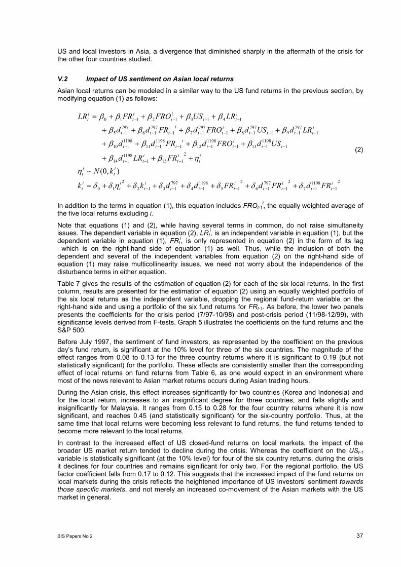
BIS Papers No 2 37
US and local investors in Asia, a divergence that diminished sharply in the aftermath of the crisis forthe other four countries studied.
V.2 Impact of US sentiment on Asian local returns
Asian local returns can be modeled in a similar way to the US fund returns in the previous section, bymodifying equation (1) as follows:
21
119817
21
79716
215
119814
7971312
210
21151
1198114
111981131
11981121
1198111
1198110
1797191
797181
797171
79716
79715
141312110
),0(~itt
itt
ittt
it
it
it
it
it
it
it
itt
ttitt
ittt
itttt
itt
ittt
itt
it
it
it
FRdFRdFRddkk
kNFRLRd
USdFROdFRdd
LRdUSdFROdFRdd
LRUSFROFRLR
(2)
In addition to the terms in equation (1), this equation includes FROt-1i, the equally weighted average of
the five local returns excluding i.
Note that equations (1) and (2), while having several terms in common, do not raise simultaneityissues. The dependent variable in equation (2), LRt
i, is an independent variable in equation (1), but thedependent variable in equation (1), FRt
i, is only represented in equation (2) in the form of its lag- which is on the right-hand side of equation (1) as well. Thus, while the inclusion of both thedependent and several of the independent variables from equation (2) on the right-hand side ofequation (1) may raise multicollinearity issues, we need not worry about the independence of thedisturbance terms in either equation.
Table 7 gives the results of the estimation of equation (2) for each of the six local returns. In the firstcolumn, results are presented for the estimation of equation (2) using an equally weighted portfolio ofthe six local returns as the independent variable, dropping the regional fund-return variable on theright-hand side and using a portfolio of the six fund returns for FRt-1. As before, the lower two panelspresents the coefficients for the crisis period (7/97-10/98) and post-crisis period (11/98-12/99), withsignificance levels derived from F-tests. Graph 5 illustrates the coefficients on the fund returns and theS&P 500.
Before July 1997, the sentiment of fund investors, as represented by the coefficient on the previousdays fund return, is significant at the 10% level for three of the six countries. The magnitude of theeffect ranges from 0.08 to 0.13 for the three country returns where it is significant to 0.19 (but notstatistically significant) for the portfolio. These effects are consistently smaller than the correspondingeffect of local returns on fund returns from Table 6, as one would expect in an environment wheremost of the news relevant to Asian market returns occurs during Asian trading hours.
During the Asian crisis, this effect increases significantly for two countries (Korea and Indonesia) andfor the local return, increases to an insignificant degree for three countries, and falls slightly andinsignificantly for Malaysia. It ranges from 0.15 to 0.28 for the four country returns where it is nowsignificant, and reaches 0.45 (and statistically significant) for the six-country portfolio. Thus, at thesame time that local returns were becoming less relevant to fund returns, the fund returns tended tobecome more relevant to the local returns.
In contrast to the increased effect of US closed-fund returns on local markets, the impact of thebroader US market return tended to decline during the crisis. Whereas the coefficient on the USt-1variable is statistically significant (at the 10% level) for four of the six country returns, during the crisisit declines for four countries and remains significant for only two. For the regional portfolio, the USfactor coefficient falls from 0.17 to 0.12. This suggests that the increased impact of the fund returns onlocal markets during the crisis reflects the heightened importance of US investors sentiment towardsthose specific markets, and not merely an increased co-movement of the Asian markets with the USmarket in general.

38 BIS Papers No 2
After the crisis, the fund-return coefficient tends to fall again. In fact, the fund return is significant andpositive for only one local market (the Philippines), compared with three before and four during thecrisis; it turns significant and negative for Malaysia. For the regional portfolio, the fund-returncoefficient remains significant after the crisis, but declines to 0.13.
Meanwhile, the influence of the broad US market return again rises after October 1998 for four of thesix countries. It becomes significant at the 5% level for five of them - all except Taiwan, one of the onlytwo where it had been significant during the crisis. For the regional portfolio, the coefficient on theS&P 500 return rises to 0.39.
V.3 Summary
A number of stylised facts can be drawn from the results in the previous two sections. During normaltimes, Asian market returns and closed-end fund returns influence each other, but the effect of theAsian returns on the funds is the greater. During the Asian crisis, the effect of the Asian markets onthe funds declines, while that of the funds on the Asian markets increases. Movements in the S&P 500(a proxy for the US market as a whole) become more important for the fund returns during the Asiancrisis, but have a reduced impact on the Asian local markets (even as their indirect impact via thefunds increases). After the crisis, the direction of causality again seems to go from the Asian localmarkets to the country funds, with effects in the reverse direction in most cases even weaker thanbefore. The influence of the broader US market declines, but remains somewhat stronger than it hadbeen before the crisis.
VI. Tracking the direction of influence: daily volatilityThe previous section attempted to determine whether and in what ways the flow of news betweenthe US and Asian markets changed during the Asian crisis, by looking at changes in market and fundreturns. Another form of news, however, is volatility. An increase of price volatility in a given marketcould indicate a wider divergence of views among investors, increased activity by a previously passivegroup of investors, or a deterioration in liquidity conditions. When increased volatility in one marketreturn is followed by increased volatility in a related return, after the assumed determinants of the tworeturns are accounted for, this could indicate that news about participation, liquidity, or changes ofopinion in one market is relevant to market values in the other market.
Lagrange multiplier (LM) tests (available from the authors) confirm that, for all of the countries studied,the mean equations in systems (1) and (2) are characterised by autoregressive conditionalheteroskedasticity. Using this fact, this section attempts to determine whether volatility is linked acrossregions - ie whether an unusually volatile day in one market is followed by an unusually volatile day inthe other - and whether and how these patterns changed during the crisis period.
The GARCH(1,1) specifications in equations (1) and (2) enable us to ask a number of questions aboutthe volatility of country-fund and local market returns. The coefficients on the time-period dummies inthe variance equation of system (1) ( and ) indicate whether volatility as a whole was higher duringthose periods compared with January 1995-June 1997. The coefficient on the squared local return ()in the variance equation indicates whether volatile market returns in Asia are followed by volatilereturns on the corresponding country-funds in New York, irrespective of its effects on the levels of thereturns. The coefficients on the interaction terms ( and ) indicate whether volatility transfer wasaccentuated or dampened during these periods. The analogous interpretations hold for the coefficients in system (2).
Tables 8 and 9 present the estimated coefficients of the variance equations in (1) and (2). FromJanuary 1995 through June 1997, volatility tended to be transmitted strongly from the local markets tothe country funds, but not vice versa. The squared local return has a positive, significant effect (at a10% confidence level) on fund volatility for four of the six countries and for the six-country portfolio(Table 8). This effect changes somewhat for some of the national markets during the crisis andpost-crisis periods, but generally not in a strong or consistent way. It rises for three countries (onesignificantly) after July 1997, then falls for four countries (two significantly, with a significant rise forMalaysia) after November 1998.
In contrast, the transmission of volatility from the funds to the Asian market did seem to change overthe course of the sample period (Table 9). The squared fund return has a positive and significant effecton local-return volatility during the pre-crisis period for only one country (Malaysia). During the crisis,

BIS Papers No 2 39
this coefficient rises for five of the six countries, and becomes significant for three of them (although,puzzlingly, despite rising it is no longer significant for Malaysia). After the crisis, it declines for fourcountries, and remains significant and positive for only two of them, while becoming significantlynegative for Malaysia.
The overall picture that emerges, although clouded by divergent results in certain countries, can bestated as follows. Before July 1997, volatility in local returns was strongly transmitted to country funds,while volatility transmission in the reverse direction was weaker. During the crisis, volatility tended tobe transmitted strongly in both directions. After the crisis, volatility transmission in both directionstended to decline, and indeed was lower than before the crisis in most cases. This suggests that, tothe extent that country-fund returns reflect the sentiment of US investors towards the Asian markets,this sentiment was much more important for market developments during the crisis than before orafter. Local Asian market developments were about equally important for US sentiment regarding Asiabefore, during and after the crisis period.
There are two notable, and instructive, exceptions to this pattern. For Taiwan, volatility transmission inboth directions was insignificant in the pre-crisis period and increased throughout the time understudy. The volatility of the Taiwan fund return becomes significant and positive for local-return volatilityin the post-crisis period. As already noted, Taiwan escaped the worst effects of the crisis. It is possiblethat, as western investors sought opportunities in the region in the aftermath of the crisis, Taiwan wasseen as an especially promising market, strengthening linkages between western sentiment and localreturns.
The other key exception is Malaysia, where the influence of local-return volatility on that of fundreturns rose strongly after the crisis, while volatility transmisssion in the opposite direction becomessignificantly negative (though small in absolute terms). These findings may reflect the imposition ofcapital controls in September 1998, as a result of which foreign holders of Malaysian shares wereheavily affected by local returns but could do little to influence these returns by reallocating theirportfolios. The low coefficient on fund-return volatility for the local return may thus reflect Malaysiasability to insulate itself from foreign investor sentiment, while the high coefficient on volatilitytransmission in the opposite direction reflects the continuing interest that US investors had in localdevelopments.
VII. Market sentiment and flows into Asian equitiesChanges in sentiment between different classes of investors ought to be associated with portfolioshifts: we would expect investors who have become optimistic about a securitys future returns topurchase it from those who are (or have become) pessimistic. Similarly, price changes that are notassociated with portfolio shifts might indicate that all classes of investors have experienced a parallelshift in opinion. This section asks whether changes in US investor holdings of Asian equities wereassociated with differences in sentiment about Asian market prospects, using thelocal-return/fund-return relationship as an indicator of these differences in sentiment.
US purchases of Asian equities are measured using data from State Street Bank and Trust Co, a largeUS-based custodian of foreign securities. At August 1998, State Street was estimated to be thecustodian for 40% of the securities holdings of US mutual funds (Froot et al, 1998). The data used inthis study are net equity purchases and sales settled in the corresponding Asian currency, where thetransaction is initiated by non-local investors. Thus, while these figures obviously do not account for allforeign purchases and shares of Asian equities, they are likely to offer a useful indicator of the sizeand direction of these flows.
Monthly figures were available on net purchases of equities by non-local investors in five of the sixcountries studied above (all except Taiwan). These were divided by the total capitalisation of thecorresponding national stock market to obtain a capital-inflow indicator, summarised in Table 10 andGraph 6. One fact immediately apparent from these data is that they do not correspond neatly to thecrisis period - while investors did engage in sustained selling over certain crisis periods from certaincountries (for example, sales of Indonesian equities were high in the first months of 1998), one cannotestablish a clear link between increased sales of Asian equities by foreign investors and the onset orpersistence of crisis conditions in the Asian markets. The volatility of equity flows is generally higherduring the crisis period than before or after, though even this is not the case for Indonesia and thePhilippines.
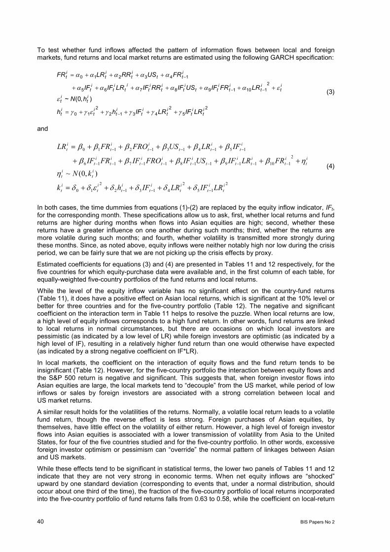
40 BIS Papers No 2
To test whether fund inflows affected the pattern of information flows between local and foreignmarkets, fund returns and local market returns are estimated using the following GARCH specification:
25
24312
210
2110198765
143210
),0(~it
it
it
it
it
it
it
it
it
it
it
it
itt
it
it
it
it
it
it
itt
it
it
it
LRIFLRIFhh
hN
LRFRIFUSIFRRIFLRIFIF
FRUSRRLRFR
(3)
and
215
241312
210
2110119118117116
15141312110
),0(~it
it
it
it
it
it
it
it
it
it
it
it
itt
it
it
it
it
it
it
itt
it
it
it
LRIFLRIFhk
kNFRLRIFUSIFFROIFFRIF
IFLRUSFROFRLR
(4)
In both cases, the time dummies from equations (1)-(2) are replaced by the equity inflow indicator, IFt,for the corresponding month. These specifications allow us to ask, first, whether local returns and fundreturns are higher during months when flows into Asian equities are high; second, whether thesereturns have a greater influence on one another during such months; third, whether the returns aremore volatile during such months; and fourth, whether volatility is transmitted more strongly duringthese months. Since, as noted above, equity inflows were neither notably high nor low during the crisisperiod, we can be fairly sure that we are not picking up the crisis effects by proxy.
Estimated coefficients for equations (3) and (4) are presented in Tables 11 and 12 respectively, for thefive countries for which equity-purchase data were available and, in the first column of each table, forequally-weighted five-country portfolios of the fund returns and local returns.
While the level of the equity inflow variable has no significant effect on the country-fund returns(Table 11), it does have a positive effect on Asian local returns, which is significant at the 10% level orbetter for three countries and for the five-country portfolio (Table 12). The negative and significantcoefficient on the interaction term in Table 11 helps to resolve the puzzle. When local returns are low,a high level of equity inflows corresponds to a high fund return. In other words, fund returns are linkedto local returns in normal circumstances, but there are occasions on which local investors arepessimistic (as indicated by a low level of LR) while foreign investors are optimistic (as indicated by ahigh level of IF), resulting in a relatively higher fund return than one would otherwise have expected(as indicated by a strong negative coefficient on IF*LR).
In local markets, the coefficient on the interaction of equity flows and the fund return tends to beinsignificant (Table 12). However, for the five-country portfolio the interaction between equity flows andthe S&P 500 return is negative and significant. This suggests that, when foreign investor flows intoAsian equities are large, the local markets tend to decouple from the US market, while period of lowinflows or sales by foreign investors are associated with a strong correlation between local andUS market returns.
A similar result holds for the volatilities of the returns. Normally, a volatile local return leads to a volatilefund return, though the reverse effect is less strong. Foreign purchases of Asian equities, bythemselves, have little effect on the volatility of either return. However, a high level of foreign investorflows into Asian equities is associated with a lower transmission of volatility from Asia to the UnitedStates, for four of the five countries studied and for the five-country portfolio. In other words, excessiveforeign investor optimism or pessimism can override the normal pattern of linkages between Asianand US markets.
While these effects tend to be significant in statistical terms, the lower two panels of Tables 11 and 12indicate that they are not very strong in economic terms. When net equity inflows are shockedupward by one standard deviation (corresponding to events that, under a normal distribution, shouldoccur about one third of the time), the fraction of the five-country portfolio of local returns incorporatedinto the five-country portfolio of fund returns falls from 0.63 to 0.58, while the coefficient on local-return
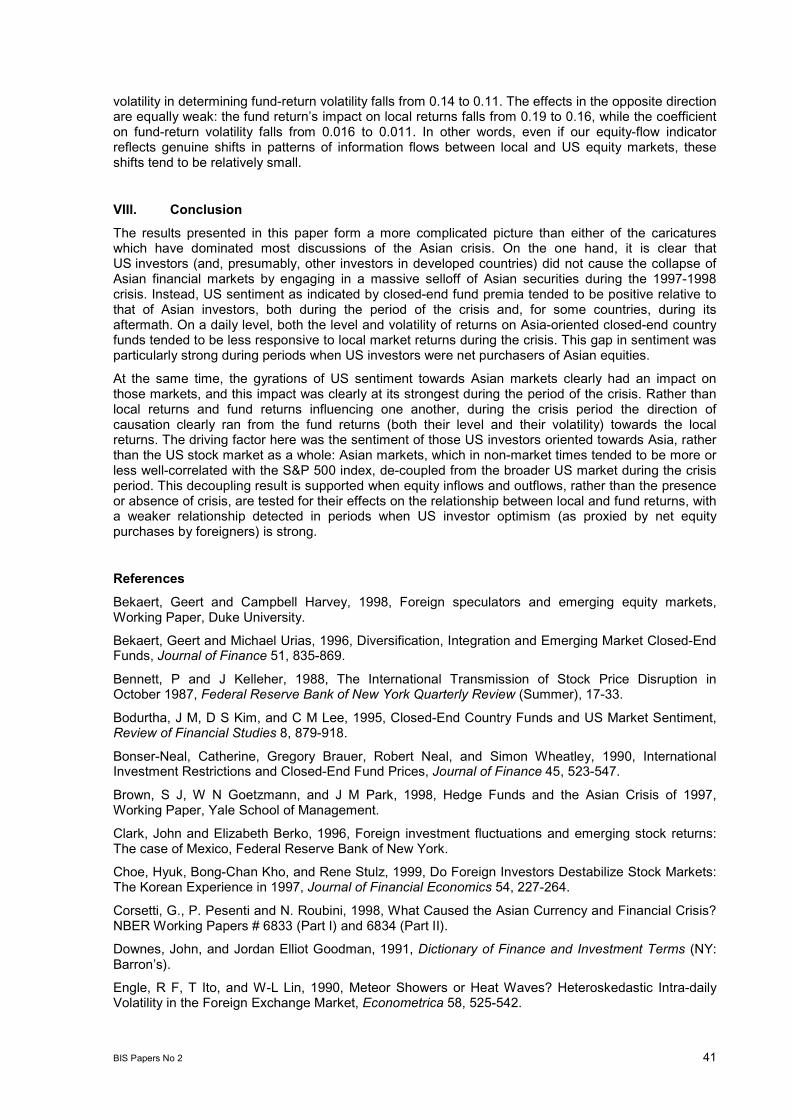
BIS Papers No 2 41
volatility in determining fund-return volatility falls from 0.14 to 0.11. The effects in the opposite directionare equally weak: the fund returns impact on local returns falls from 0.19 to 0.16, while the coefficienton fund-return volatility falls from 0.016 to 0.011. In other words, even if our equity-flow indicatorreflects genuine shifts in patterns of information flows between local and US equity markets, theseshifts tend to be relatively small.
VIII. ConclusionThe results presented in this paper form a more complicated picture than either of the caricatureswhich have dominated most discussions of the Asian crisis. On the one hand, it is clear thatUS investors (and, presumably, other investors in developed countries) did not cause the collapse ofAsian financial markets by engaging in a massive selloff of Asian securities during the 1997-1998crisis. Instead, US sentiment as indicated by closed-end fund premia tended to be positive relative tothat of Asian investors, both during the period of the crisis and, for some countries, during itsaftermath. On a daily level, both the level and volatility of returns on Asia-oriented closed-end countryfunds tended to be less responsive to local market returns during the crisis. This gap in sentiment wasparticularly strong during periods when US investors were net purchasers of Asian equities.
At the same time, the gyrations of US sentiment towards Asian markets clearly had an impact onthose markets, and this impact was clearly at its strongest during the period of the crisis. Rather thanlocal returns and fund returns influencing one another, during the crisis period the direction ofcausation clearly ran from the fund returns (both their level and their volatility) towards the localreturns. The driving factor here was the sentiment of those US investors oriented towards Asia, ratherthan the US stock market as a whole: Asian markets, which in non-market times tended to be more orless well-correlated with the S&P 500 index, de-coupled from the broader US market during the crisisperiod. This decoupling result is supported when equity inflows and outflows, rather than the presenceor absence of crisis, are tested for their effects on the relationship between local and fund returns, witha weaker relationship detected in periods when US investor optimism (as proxied by net equitypurchases by foreigners) is strong.
ReferencesBekaert, Geert and Campbell Harvey, 1998, Foreign speculators and emerging equity markets,Working Paper, Duke University.
Bekaert, Geert and Michael Urias, 1996, Diversification, Integration and Emerging Market Closed-EndFunds, Journal of Finance 51, 835-869.
Bennett, P and J Kelleher, 1988, The International Transmission of Stock Price Disruption inOctober 1987, Federal Reserve Bank of New York Quarterly Review (Summer), 17-33.
Bodurtha, J M, D S Kim, and C M Lee, 1995, Closed-End Country Funds and US Market Sentiment,Review of Financial Studies 8, 879-918.
Bonser-Neal, Catherine, Gregory Brauer, Robert Neal, and Simon Wheatley, 1990, InternationalInvestment Restrictions and Closed-End Fund Prices, Journal of Finance 45, 523-547.
Brown, S J, W N Goetzmann, and J M Park, 1998, Hedge Funds and the Asian Crisis of 1997,Working Paper, Yale School of Management.
Clark, John and Elizabeth Berko, 1996, Foreign investment fluctuations and emerging stock returns:The case of Mexico, Federal Reserve Bank of New York.
Choe, Hyuk, Bong-Chan Kho, and Rene Stulz, 1999, Do Foreign Investors Destabilize Stock Markets:The Korean Experience in 1997, Journal of Financial Economics 54, 227-264.
Corsetti, G., P. Pesenti and N. Roubini, 1998, What Caused the Asian Currency and Financial Crisis?NBER Working Papers # 6833 (Part I) and 6834 (Part II).
Downes, John, and Jordan Elliot Goodman, 1991, Dictionary of Finance and Investment Terms (NY:Barrons).
Engle, R F, T Ito, and W-L Lin, 1990, Meteor Showers or Heat Waves? Heteroskedastic Intra-dailyVolatility in the Foreign Exchange Market, Econometrica 58, 525-542.

42 BIS Papers No 2
Errunza, V, L W Senbet, and K Hogan, 1998, The Pricing of Country Funds from Emerging Markets:Theory and Evidence, International Journal of Theoretical and Applied Finance 1, 111-43.
Frankel, J and S Schmukler, 1996, Country Fund Discounts and the Mexican Crisis of December1994: Did Local Residents Turn Pessimistic before International Investors? Open EconomiesReview 7, Supplement 1, 511-34.
Froot, Kenneth A, Paul G J OConnell, and Mark Seasholes, 1998, The Portfolio Flows of InternationalInvestors I, NBER Working Paper 6687.
Glosten, L R, R Jagannathan, and D E Runkle, 1993, On the Relation between the Expected Valueand the Volatility of the Nominal Excess Return on Stocks, Journal of Finance 48, 1779-1801.
Hardouvelis, G, R La Porta, and T Wizman, 1994, What Moves the Discount on Country EquityFunds? In J Frankel (Ed.), The Internationalization of Equity Markets, Chicago and London: Universityof Chicago Press, 345-97.
King, M and S Wadhwani, 1990, Transmission of Volatility between Stock Markets, Review ofFinancial Studies 3, 5-33.
Klibanoff, P, O Lamont, and T Wizman, 1998, Investor Reaction to Salient News in Closed-EndCountry Funds, Journal of Finance 53, 673-99.
Kramer, Charles and Richard Todd Smith, 1995, Recent Turmoil in Emerging Markets and theBehavior of Country Fund Discounts: Renewing the Puzzle of the Pricing of Closed End Mutual Funds,IMF Working Paper.
Krugman, P, 1998, What Happened to Asia? Working Paper, MIT, Downloanable at:web.mit.edu/krugman/www.
Krugman, P, 1999, Balance Sheets, the Transfer Problem, and Finanancial Crises, working paper
Lee, C M, A Shleifer, and R H Thaler, 1991, Investor Sentiment and the Closed-End Fund Puzzle,Journal of Finance 46, 75-109.
Levy-Yeyati, Eduardo and Angel Ubide, 1998, Crisis, Contagion, and the Closed-End Fund Puzzle,IMF Working Paper, 1998.
Lin, W-L, R F Engle, and T Ito, 1994, Do Bulls and Bears Move across Borders? InternationalTransmission of Stock Returns and Volatility, Review of Financial Studies 7, 507-38.
McKinnon, R and H Pill, 1998, Overborrowing: A Decomposition of Credit and Currency Risks, WorldDevelopment.
Moreno, R, G Pasadilla, and E Remolona, 1998, Asias Financial Crisis: Lessons and PolicyResponses, In Asia: Responding to Crisis, Tokyo: Asian Development Bank Institute.
Tesar, Linda and Ligrid Werner, 1995, Home Bias and High Turnover, Journal of International Moneyand Finance 14, 467-492.
Wermers, R, 1998, Mutual fund herding and the impact on stock prices, Journal of Finance,forthcoming.
Wolf, M, 1998, Flows and Blows, Financial Times, 3 March 1998.

BIS Papers No 2 43
Graph 1a. Components of net portfolio investment (US$M.): Korea
-25000
-20000
-15000
-10000
-5000
0
5000
10000
1995 1996 1997 1998 1999
Net portfolio investment
Change in bank claims
Net securities issuance
Graph 1b. Components of net portfolio investment (US$M.): Thailand
-15000
-10000
-5000
0
5000
10000
15000
1995 1996 1997 1998 1999
Net portfolio investment
Change in bank claims
Net securities issuance

44 BIS Papers No 2
Graph 1c. Components of net portfolio investment (US$M): Philippines
-3000
-2000
-1000
0
1000
2000
3000
4000
1995 1996 1997 1998 1999
Net portfolio investment
Change in bank claimsNet securities issuance
Source (all graphs): IMF, BIS.

BIS Papers No 2 45
Graph 2a. Banks and equity investors compared: Korea
-25000
-20000
-15000
-10000
-5000
0
5000
10000
1995 1996 1997 1998 1999-15.00
-10.00
-5.00
0.00
5.00
10.00
15.00
20.00
25.00
30.00
Change in bank claims (US$M) (left)
Avg daily net equity purchases (bp of marketcapitalisation) (right)
Graph 2b. Banks and equity investors compared: Thailand
-20000
-15000
-10000
-5000
0
5000
10000
15000
1995 1996 1997 1998 1999-4.00
-2.00
0.00
2.00
4.00
6.00
8.00
10.00
12.00
Change in bank claims (US$M) (left)
Average daily net equity purchases (bp of marketcapitalisation) (right)
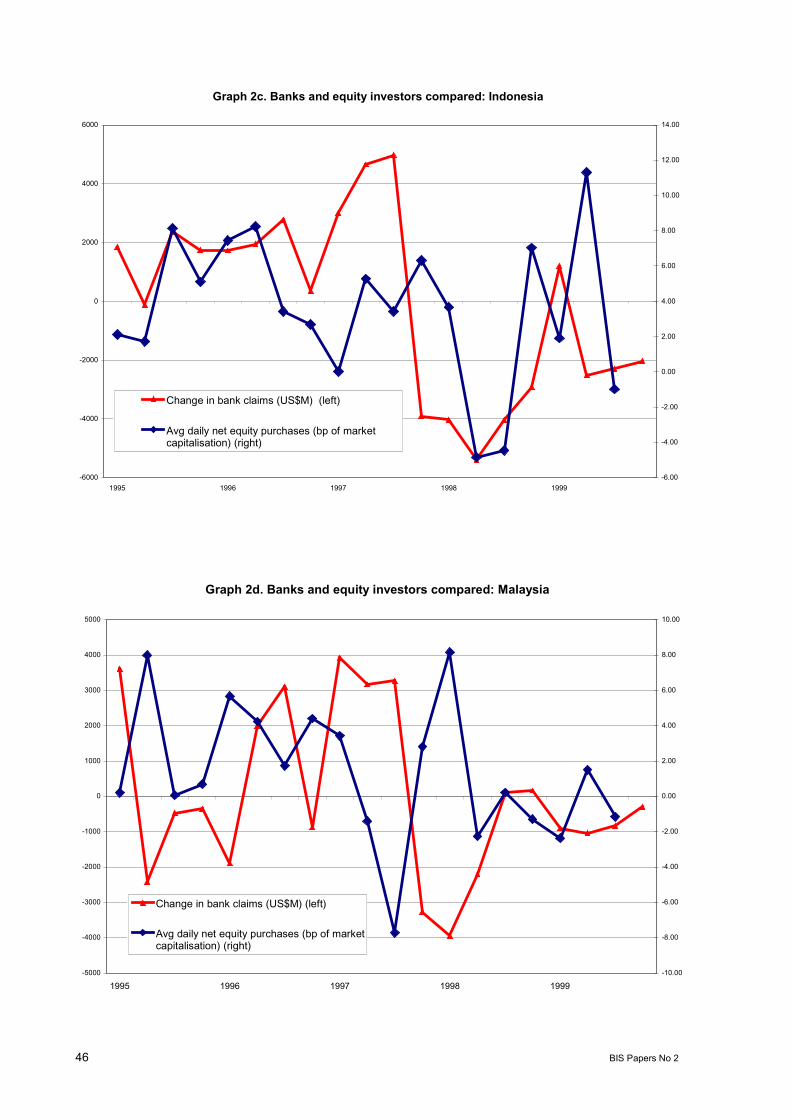
46 BIS Papers No 2
Graph 2c. Banks and equity investors compared: Indonesia
-6000
-4000
-2000
0
2000
4000
6000
1995 1996 1997 1998 1999-6.00
-4.00
-2.00
0.00
2.00
4.00
6.00
8.00
10.00
12.00
14.00
Change in bank claims (US$M) (left)
Avg daily net equity purchases (bp of marketcapitalisation) (right)
Graph 2d. Banks and equity investors compared: Malaysia
-5000
-4000
-3000
-2000
-1000
0
1000
2000
3000
4000
5000
1995 1996 1997 1998 1999-10.00
-8.00
-6.00
-4.00
-2.00
0.00
2.00
4.00
6.00
8.00
10.00
Change in bank claims (US$M) (left)
Avg daily net equity purchases (bp of marketcapitalisation) (right)
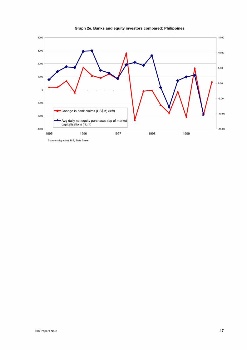
BIS Papers No 2 47
Graph 2e. Banks and equity investors compared: Philippines
-3000
-2000
-1000
0
1000
2000
3000
4000
1995 1996 1997 1998 1999-15.00
-10.00
-5.00
0.00
5.00
10.00
15.00
Change in bank claims (US$M) (left)
Avg daily net equity purchases (bp of marketcapitalisation) (right)
Source (all graphs): BIS, State Street.
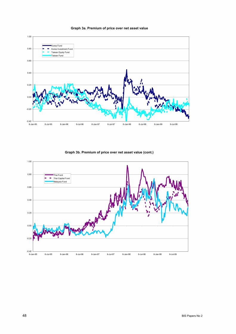
48 BIS Papers No 2
Graph 3a. Premium of price over net asset value
-0.40
-0.20
0.00
0.20
0.40
0.60
0.80
1.00
6-Jan-95 6-Jul-95 6-Jan-96 6-Jul-96 6-Jan-97 6-Jul-97 6-Jan-98 6-Jul-98 6-Jan-99 6-Jul-99
Korea FundKorea Investment FundTaiwan Equity FundTaiwan Fund
Graph 3b. Premium of price over net asset value (cont.)
-0.40
-0.20
0.00
0.20
0.40
0.60
0.80
1.00
6-Jan-95 6-Jul-95 6-Jan-96 6-Jul-96 6-Jan-97 6-Jul-97 6-Jan-98 6-Jul-98 6-Jan-99 6-Jul-99
Thai FundThai Capital FundMalaysia Fund
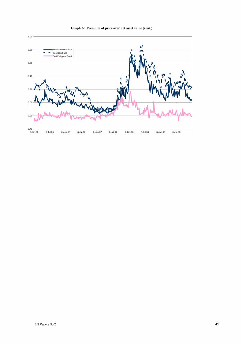
BIS Papers No 2 49
Graph 3c. Premium of price over net asset value (cont.)
-0.40
-0.20
0.00
0.20
0.40
0.60
0.80
1.00
6-Jan-95 6-Jul-95 6-Jan-96 6-Jul-96 6-Jan-97 6-Jul-97 6-Jan-98 6-Jul-98 6-Jan-99 6-Jul-99
Jakarta Growth FundIndonesia FundFirst Philippine Fund
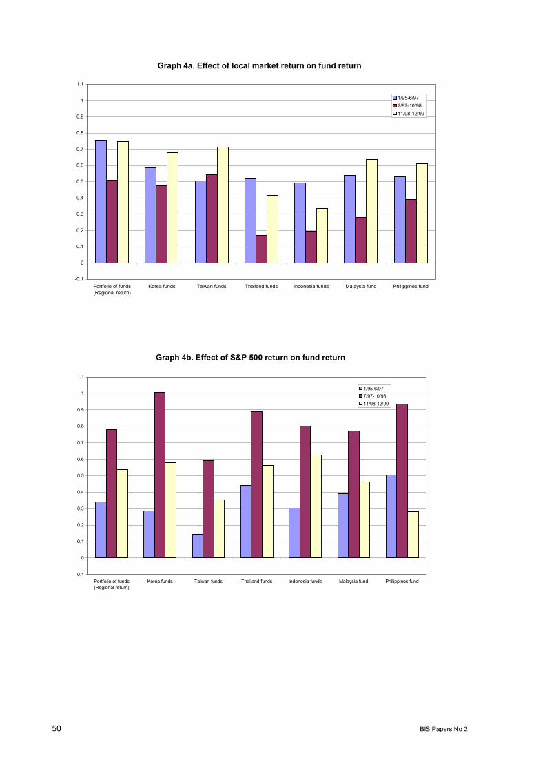
50 BIS Papers No 2
Graph 4a. Effect of local market return on fund return
-0.1
0
0.1
0.2
0.3
0.4
0.5
0.6
0.7
0.8
0.9
1
1.1
Portfolio of funds(Regional return)
Korea funds Taiwan funds Thailand funds Indonesia funds Malaysia fund Philippines fund
1/95-6/977/97-10/9811/98-12/99
Graph 4b. Effect of S&P 500 return on fund return
-0.1
0
0.1
0.2
0.3
0.4
0.5
0.6
0.7
0.8
0.9
1
1.1
Portfolio of funds(Regional return)
Korea funds Taiwan funds Thailand funds Indonesia funds Malaysia fund Philippines fund
1/95-6/977/97-10/9811/98-12/99
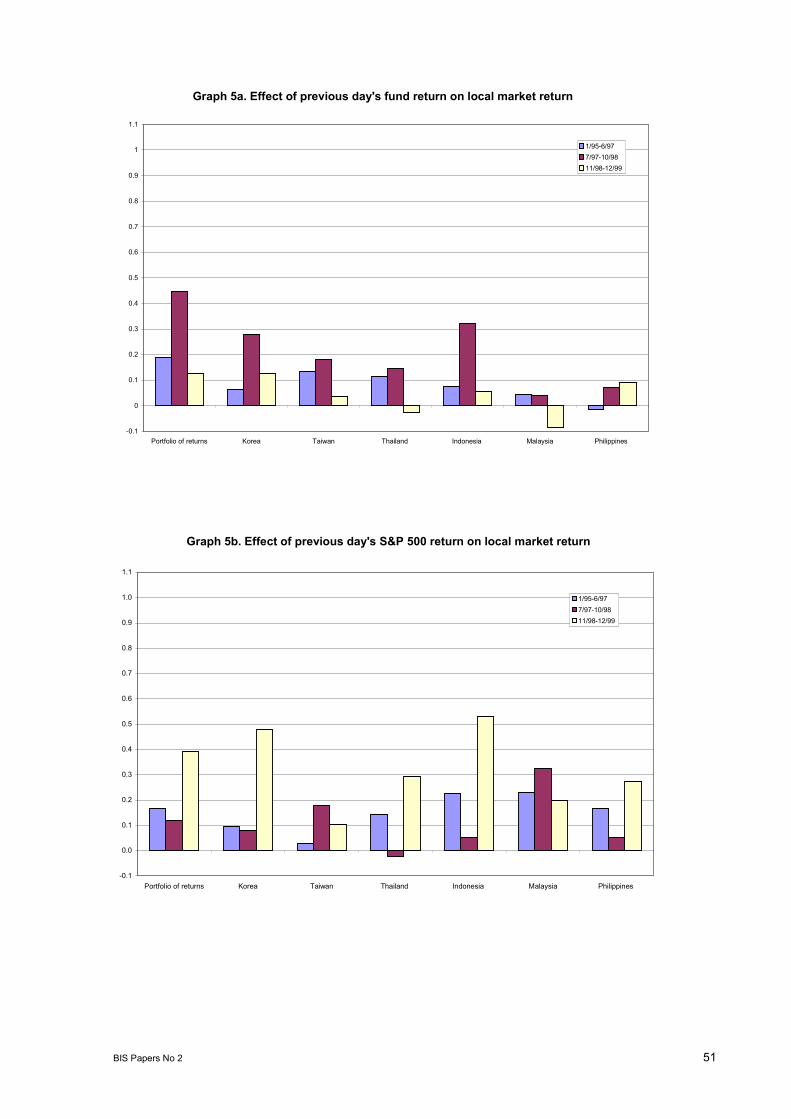
BIS Papers No 2 51
Graph 5a. Effect of previous day's fund return on local market return
-0.1
0
0.1
0.2
0.3
0.4
0.5
0.6
0.7
0.8
0.9
1
1.1
Portfolio of returns Korea Taiwan Thailand Indonesia Malaysia Philippines
1/95-6/977/97-10/9811/98-12/99
Graph 5b. Effect of previous day's S&P 500 return on local market return
-0.1
0.0
0.1
0.2
0.3
0.4
0.5
0.6
0.7
0.8
0.9
1.0
1.1
Portfolio of returns Korea Taiwan Thailand Indonesia Malaysia Philippines
1/95-6/977/97-10/9811/98-12/99
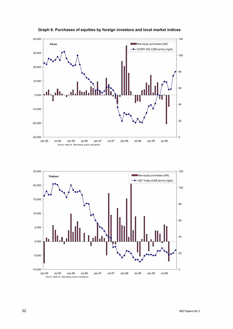
52 BIS Papers No 2
Graph 6. Purchases of equities by foreign investors and local market indices
-30.000
-20.000
-10.000
0.000
10.000
20.000
30.000
40.000
Jan.95 Jul.95 Jan.96 Jul.96 Jan.97 Jul.97 Jan.98 Jul.98 Jan.99 Jul.990
20
40
60
80
100
120
Net equity purchases (left)
KOSPI 200 (US$ terms) (right)
Source: State St., Bloomberg, author calculations.
Korea
-10.000
-5.000
0.000
5.000
10.000
15.000
20.000
25.000
Jan.95 Jul.95 Jan.96 Jul.96 Jan.97 Jul.97 Jan.98 Jul.98 Jan.99 Jul.990
20
40
60
80
100
120Net equity purchases (left)
SET Index (US$ terms) (right)
Source: State St., Bloomberg, author calculations.
Thailand
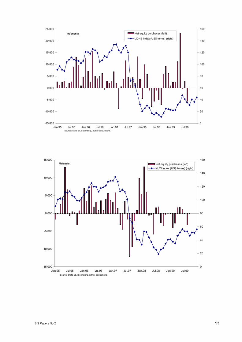
BIS Papers No 2 53
-15.000
-10.000
-5.000
0.000
5.000
10.000
15.000
20.000
25.000
Jan.95 Jul.95 Jan.96 Jul.96 Jan.97 Jul.97 Jan.98 Jul.98 Jan.99 Jul.990
20
40
60
80
100
120
140
160Net equity purchases (left)
LQ-45 Index (US$ terms) (right)
Source: State St, Bloomberg, author calculations.
Indonesia
-15.000
-10.000
-5.000
0.000
5.000
10.000
15.000
Jan.95 Jul.95 Jan.96 Jul.96 Jan.97 Jul.97 Jan.98 Jul.98 Jan.99 Jul.990
20
40
60
80
100
120
140
160Net equity purchases (left)KLCI Index (US$ terms) (right)
Source: State St., Bloomberg, author calculations.
Malaysia
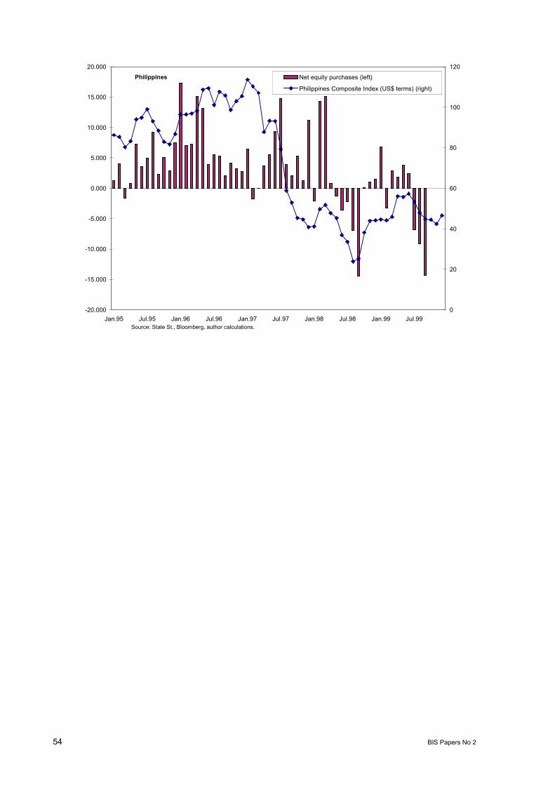
54 BIS Papers No 2
-20.000
-15.000
-10.000
-5.000
0.000
5.000
10.000
15.000
20.000
Jan.95 Jul.95 Jan.96 Jul.96 Jan.97 Jul.97 Jan.98 Jul.98 Jan.99 Jul.990
20
40
60
80
100
120Net equity purchases (left)
Philippines Composite Index (US$ terms) (right)
Source: State St., Bloomberg, author calculations.
Philippines

BIS Papers No 2 55
Table 1Capital flows to Asian countries
(US$ bn)
1995 1996 1997 1998 1999
Indonesia
Direct investment 3.7 5.6 4.5 0.4 1.51
Portfolio investment 4.1 5.0 2.6 1.9 1.51
Other investments 2.4 0.2 0.6 1.6 0.81
Current account balance 6.4 7.7 4.9 4.1 3.91
Change in reserves 1.6 4.5 5.1 2.1 3.31
Korea
Direct investment 1.8 2.3 1.6 0.6 4.8Portfolio investment 11.6 15.2 14.3 1.9 8.8Other investments 7.5 11.1 10.8 2.1 12.7Current account balance 8.5 23.0 8.2 40.6 25.0Change in reserves 7.0 1.4 11.9 31.0 23.0
Malaysia
Direct investment 4.2 5.1 5.1Portfolio investment 0.4 0.3 0.2Other investments 3.9 4.7 2.1Current account balance 8.5 4.6 4.8 9.4 12.5Change in reserves 1.8 2.5 3.9 10.6 4.7
The Philippines
Direct investment 1.1 1.3 1.1 1.6 0.7Portfolio investment 1.2 5.3 0.6 0.9 2.8Other investments 2.7 4.3 5.3 0.9 0.41
Current account balance 2.0 4.0 4.4 1.3 7.0Change in reserves 0.9 4.0 2.6 1.9 4.0
Taiwan
Direct investment 1.4 2.0 3.0 3.6 1.5Portfolio investment 0.5 1.1 8.3 2.4 9.1Other investments 7.3 5.7 3.1 8.5 5.5Current account balance 5.5 11.0 7.8 3.4 5.9Change in reserves 3.9 1.1 0.7 4.8 18.6
Thailand
Direct investment 1.2 1.4 3.4 6.8 5.3Portfolio investment 4.1 3.5 4.4 0.0 0.8Other investments 16.6 14.5 16.2 16.6 12.2Current account balance 13.6 14.7 3.0 14.0 11.0Change in reserves 7.2 2.2 9.9 1.4 4.6
1 Up to third quarter 1999.
Sources: IMF, Balance of payments; national data.
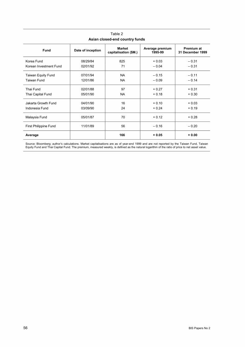
56 BIS Papers No 2
Table 2Asian closed-end country funds
Fund Date of inception Marketcapitalisation ($M.)
Average premium1995-99
Premium at31 December 1999
Korea Fund 08/29/84 825 + 0.03 0.31Korean Investment Fund 02/01/92 71 0.04 0.31
Taiwan Equity Fund 07/01/94 NA 0.15 0.11Taiwan Fund 12/01/86 NA 0.09 0.14
Thai Fund 02/01/88 97 + 0.27 + 0.31Thai Capital Fund 05/01/90 NA + 0.18 + 0.30
Jakarta Growth Fund 04/01/90 16 + 0.10 + 0.03Indonesia Fund 03/09/90 24 + 0.24 + 0.19
Malaysia Fund 05/01/87 70 + 0.12 + 0.28
First Philippine Fund 11/01/89 56 0.16 0.20
Average 166 + 0.05 + 0.00
Source: Bloomberg; authors calculations. Market capitalisations are as of year-end 1999 and are not reported by the Taiwan Fund, TaiwanEquity Fund and Thai Capital Fund. The premium, measured weekly, is defined as the natural logarithm of the ratio of price to net asset value.
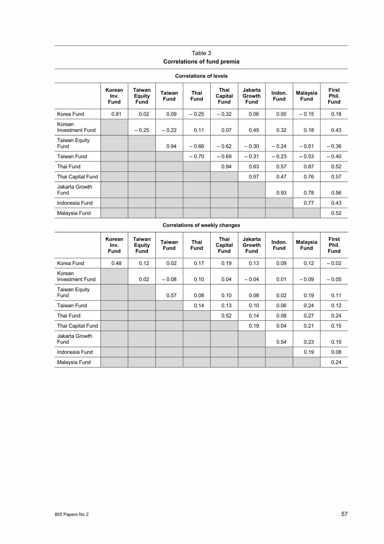
BIS Papers No 2 57
Table 3Correlations of fund premia
Correlations of levels
KoreanInv.
Fund
TaiwanEquityFund
TaiwanFund
ThaiFund
ThaiCapitalFund
JakartaGrowthFund
Indon.Fund
MalaysiaFund
FirstPhil.Fund
Korea Fund 0.81 0.02 0.09 0.25 0.32 0.06 0.00 0.15 0.18
KoreanInvestment Fund 0.25 0.22 0.11 0.07 0.45 0.32 0.18 0.43
Taiwan EquityFund 0.94 0.66 0.62 0.30 0.24 0.51 0.36
Taiwan Fund 0.70 0.69 0.31 0.23 0.53 0.40
Thai Fund 0.94 0.63 0.57 0.87 0.52
Thai Capital Fund 0.57 0.47 0.76 0.57
Jakarta GrowthFund 0.93 0.78 0.56
Indonesia Fund 0.77 0.43
Malaysia Fund 0.52
Correlations of weekly changes
KoreanInv.
Fund
TaiwanEquityFund
TaiwanFund
ThaiFund
ThaiCapitalFund
JakartaGrowthFund
Indon.Fund
MalaysiaFund
FirstPhil.Fund
Korea Fund 0.48 0.12 0.02 0.17 0.19 0.13 0.09 0.12 0.02
KoreanInvestment Fund 0.02 0.08 0.10 0.04 0.04 0.01 0.09 0.05
Taiwan EquityFund 0.57 0.08 0.10 0.08 0.02 0.19 0.11
Taiwan Fund 0.14 0.13 0.10 0.06 0.24 0.12
Thai Fund 0.52 0.14 0.08 0.27 0.24
Thai Capital Fund 0.19 0.04 0.21 0.15
Jakarta GrowthFund 0.54 0.23 0.15
Indonesia Fund 0.19 0.08
Malaysia Fund 0.24
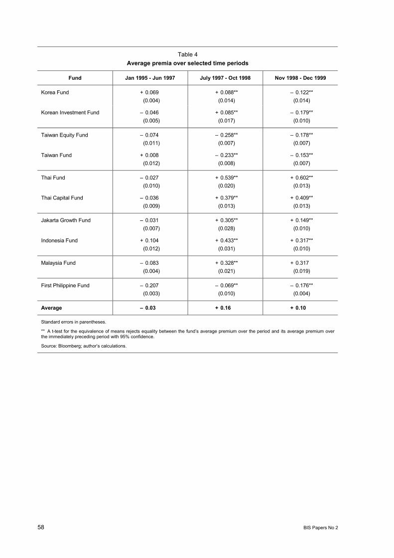
58 BIS Papers No 2
Table 4Average premia over selected time periods
Fund Jan 1995 - Jun 1997 July 1997 - Oct 1998 Nov 1998 - Dec 1999
Korea Fund + 0.069(0.004)
+ 0.088**(0.014)
0.122**(0.014)
Korean Investment Fund 0.046(0.005)
+ 0.085**(0.017)
0.179**(0.010)
Taiwan Equity Fund 0.074(0.011)
0.258**(0.007)
0.178**(0.007)
Taiwan Fund + 0.008(0.012)
0.233**(0.008)
0.153**(0.007)
Thai Fund 0.027(0.010)
+ 0.539**(0.020)
+ 0.602**(0.013)
Thai Capital Fund 0.036(0.009)
+ 0.379**(0.013)
+ 0.409**(0.013)
Jakarta Growth Fund 0.031(0.007)
+ 0.305**(0.028)
+ 0.149**(0.010)
Indonesia Fund + 0.104(0.012)
+ 0.433**(0.031)
+ 0.317**(0.010)
Malaysia Fund 0.083(0.004)
+ 0.328**(0.021)
+ 0.317(0.019)
First Philippine Fund 0.207(0.003)
0.069**(0.010)
0.176**(0.004)
Average 0.03 + 0.16 + 0.10
Standard errors in parentheses.
** A t-test for the equivalence of means rejects equality between the funds average premium over the period and its average premium overthe immediately preceding period with 95% confidence.
Source: Bloomberg; authors calculations.

BIS Papers No 2 59
Table 5Local stock markets: capitalisation data and indices used in daily regressions
Market capitalisation(US$bn)Country
End-1994 End-1999Index Number of index
members
Korea 192 309 KOSPI 200 Index 200
Taiwan 247 376 TWSE Weighted Index 452
Thailand 131 58 Bangkok SET Index 394
Indonesia 47 64 Jakarta LQ-45 Index 45
Malaysia 199 145 KL Composite Index 100
Philippines 56 48 Philippines Composite Index 33
Source: IFC; Bloomberg.
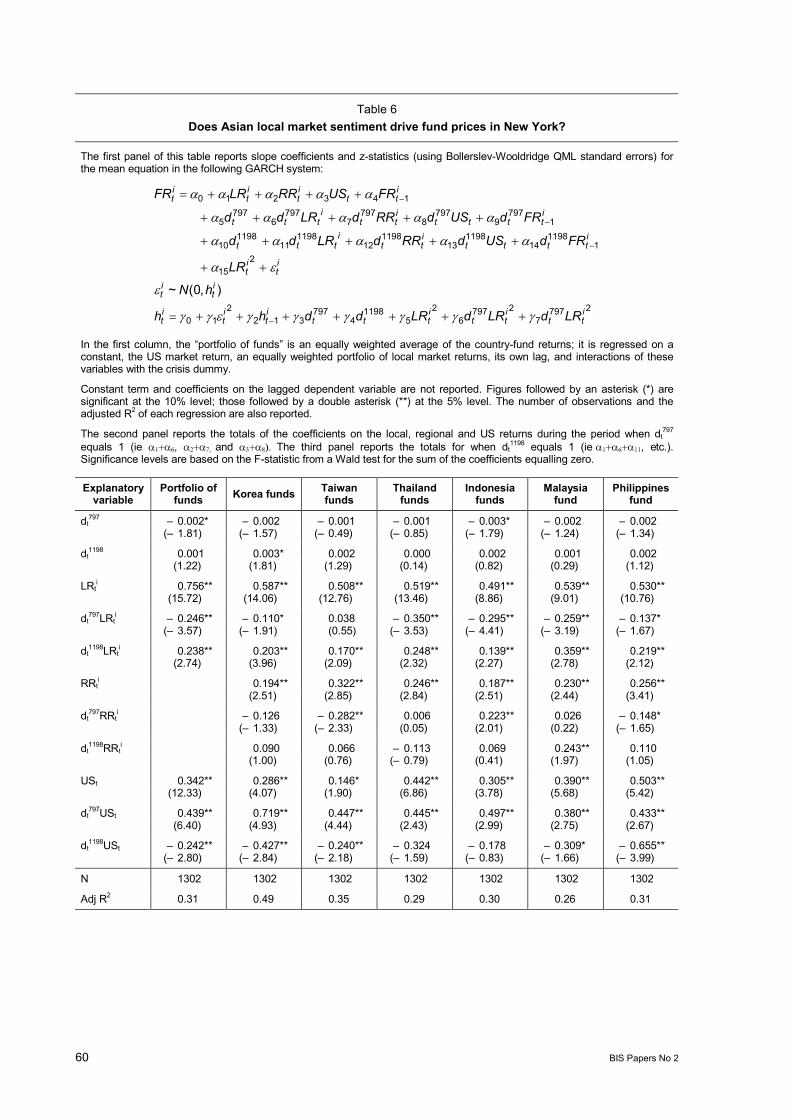
60 BIS Papers No 2
Table 6Does Asian local market sentiment drive fund prices in New York?
The first panel of this table reports slope coefficients and z-statistics (using Bollerslev-Wooldridge QML standard errors) forthe mean equation in the following GARCH system:
27977
27976
25
11984
797312
210
215
11198
141198
131198
121198
111198
10
1797
9797
8797
7797
6797
5
143210
),0(~itt
itt
ittt
it
it
it
it
it
it
it
itttt
itt
ittt
itttt
itt
ittt
itt
it
it
it
LRdLRdLRddhh
hN
LR
FRdUSdRRdLRdd
FRdUSdRRdLRdd
FRUSRRLRFR
In the first column, the portfolio of funds is an equally weighted average of the country-fund returns; it is regressed on aconstant, the US market return, an equally weighted portfolio of local market returns, its own lag, and interactions of thesevariables with the crisis dummy.
Constant term and coefficients on the lagged dependent variable are not reported. Figures followed by an asterisk (*) aresignificant at the 10% level; those followed by a double asterisk (**) at the 5% level. The number of observations and theadjusted R2 of each regression are also reported.
The second panel reports the totals of the coefficients on the local, regional and US returns during the period when dt797
equals 1 (ie , and The third panel reports the totals for when dt1198 equals 1 (ie , etc.).
Significance levels are based on the F-statistic from a Wald test for the sum of the coefficients equalling zero.
Explanatoryvariable
Portfolio offunds Korea funds Taiwan
fundsThailand
fundsIndonesia
fundsMalaysia
fundPhilippines
fund
dt797 0.002* 0.002 0.001 0.001 0.003* 0.002 0.002
( 1.81) ( 1.57) ( 0.49) ( 0.85) ( 1.79) ( 1.24) ( 1.34)
dt1198 0.001 0.003* 0.002 0.000 0.002 0.001 0.002
(1.22) (1.81) (1.29) (0.14) (0.82) (0.29) (1.12)
LRti 0.756** 0.587** 0.508** 0.519** 0.491** 0.539** 0.530**
(15.72) (14.06) (12.76) (13.46) (8.86) (9.01) (10.76)
dt797LRt
i 0.246** 0.110* 0.038 0.350** 0.295** 0.259** 0.137*( 3.57) ( 1.91) (0.55) ( 3.53) ( 4.41) ( 3.19) ( 1.67)
dt1198LRt
i 0.238** 0.203** 0.170** 0.248** 0.139** 0.359** 0.219**(2.74) (3.96) (2.09) (2.32) (2.27) (2.78) (2.12)
RRti 0.194** 0.322** 0.246** 0.187** 0.230** 0.256**
(2.51) (2.85) (2.84) (2.51) (2.44) (3.41)
dt797RRt
i 0.126 0.282** 0.006 0.223** 0.026 0.148*( 1.33) ( 2.33) (0.05) (2.01) (0.22) ( 1.65)
dt1198RRt
i 0.090 0.066 0.113 0.069 0.243** 0.110(1.00) (0.76) ( 0.79) (0.41) (1.97) (1.05)
USt 0.342** 0.286** 0.146* 0.442** 0.305** 0.390** 0.503**(12.33) (4.07) (1.90) (6.86) (3.78) (5.68) (5.42)
dt797USt 0.439** 0.719** 0.447** 0.445** 0.497** 0.380** 0.433**
(6.40) (4.93) (4.44) (2.43) (2.99) (2.75) (2.67)
dt1198USt 0.242** 0.427** 0.240** 0.324 0.178 0.309* 0.655**
( 2.80) ( 2.84) ( 2.18) ( 1.59) ( 0.83) ( 1.66) ( 3.99)
N 1302 1302 1302 1302 1302 1302 1302
Adj R2 0.31 0.49 0.35 0.29 0.30 0.26 0.31

BIS Papers No 2 61
Table 6 (contd)
Effects during 07/97 - 10/98:
LRti 0.511** 0.477** 0.546** 0.169* 0.196** 0.280** 0.393**
RRti 0.068 0.040 0.252** 0.410** 0.256** 0.108**
USt 0.781** 1.005** 0.592** 0.887** 0.803** 0.770** 0.936**
Effects during 11/98 - 12/99:
LRti 0.749** 0.679** 0.716** 0.417** 0.335** 0.639** 0.612**
RRti 0.158** 0.106 0.139 0.479** 0.499** 0.218**
USt 0.538** 0.579** 0.352** 0.563** 0.624** 0.461** 0.281**
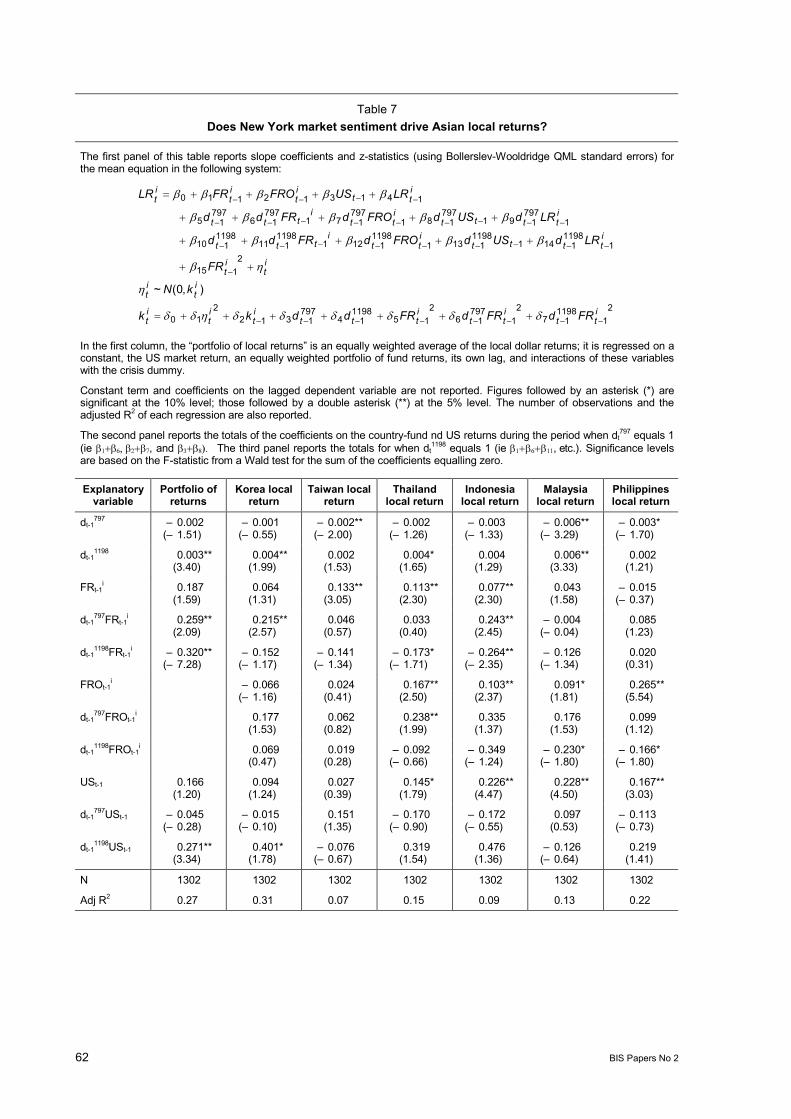
62 BIS Papers No 2
Table 7Does New York market sentiment drive Asian local returns?
The first panel of this table reports slope coefficients and z-statistics (using Bollerslev-Wooldridge QML standard errors) forthe mean equation in the following system:
21
119817
21
79716
215
119814
7971312
210
2115
11198
11411198
11311198
11211198
1111198
110
1797
191797
181797
171797
16797
15
141312110
),0(~
itt
itt
ittt
it
it
it
it
it
it
it
itttt
itt
ittt
itttt
itt
ittt
itt
it
it
it
FRdFRdFRddkk
kN
FR
LRdUSdFROdFRdd
LRdUSdFROdFRdd
LRUSFROFRLR
In the first column, the portfolio of local returns is an equally weighted average of the local dollar returns; it is regressed on aconstant, the US market return, an equally weighted portfolio of fund returns, its own lag, and interactions of these variableswith the crisis dummy.
Constant term and coefficients on the lagged dependent variable are not reported. Figures followed by an asterisk (*) aresignificant at the 10% level; those followed by a double asterisk (**) at the 5% level. The number of observations and theadjusted R2 of each regression are also reported.
The second panel reports the totals of the coefficients on the country-fund nd US returns during the period when dt797 equals 1
(ie , and The third panel reports the totals for when dt1198 equals 1 (ie , etc.). Significance levels
are based on the F-statistic from a Wald test for the sum of the coefficients equalling zero.
Explanatoryvariable
Portfolio ofreturns
Korea localreturn
Taiwan localreturn
Thailandlocal return
Indonesialocal return
Malaysialocal return
Philippineslocal return
dt-1797 0.002 0.001 0.002** 0.002 0.003 0.006** 0.003*
( 1.51) ( 0.55) ( 2.00) ( 1.26) ( 1.33) ( 3.29) ( 1.70)
dt-11198 0.003** 0.004** 0.002 0.004* 0.004 0.006** 0.002
(3.40) (1.99) (1.53) (1.65) (1.29) (3.33) (1.21)
FRt-1i 0.187 0.064 0.133** 0.113** 0.077** 0.043 0.015
(1.59) (1.31) (3.05) (2.30) (2.30) (1.58) ( 0.37)
dt-1797FRt-1
i 0.259** 0.215** 0.046 0.033 0.243** 0.004 0.085(2.09) (2.57) (0.57) (0.40) (2.45) ( 0.04) (1.23)
dt-11198FRt-1
i 0.320** 0.152 0.141 0.173* 0.264** 0.126 0.020( 7.28) ( 1.17) ( 1.34) ( 1.71) ( 2.35) ( 1.34) (0.31)
FROt-1i 0.066 0.024 0.167** 0.103** 0.091* 0.265**
( 1.16) (0.41) (2.50) (2.37) (1.81) (5.54)
dt-1797FROt-1
i 0.177 0.062 0.238** 0.335 0.176 0.099(1.53) (0.82) (1.99) (1.37) (1.53) (1.12)
dt-11198FROt-1
i 0.069 0.019 0.092 0.349 0.230* 0.166*(0.47) (0.28) ( 0.66) ( 1.24) ( 1.80) ( 1.80)
USt-1 0.166 0.094 0.027 0.145* 0.226** 0.228** 0.167**(1.20) (1.24) (0.39) (1.79) (4.47) (4.50) (3.03)
dt-1797USt-1 0.045 0.015 0.151 0.170 0.172 0.097 0.113
( 0.28) ( 0.10) (1.35) ( 0.90) ( 0.55) (0.53) ( 0.73)
dt-11198USt-1 0.271** 0.401* 0.076 0.319 0.476 0.126 0.219
(3.34) (1.78) ( 0.67) (1.54) (1.36) ( 0.64) (1.41)
N 1302 1302 1302 1302 1302 1302 1302
Adj R2 0.27 0.31 0.07 0.15 0.09 0.13 0.22

BIS Papers No 2 63
Table 7 (contd)
Effects during 7/97 - 10/98:
FRt-1I 0.446** 0.280** 0.179** 0.147** 0.320** 0.039 0.070
FROt-1I 0.111 0.086* 0.405** 0.438* 0.267** 0.365**
USt-1 0.121 0.079 0.178** 0.025 0.054 0.324* 0.054
Effects during 11/98 - 12/99:
FRt-1I 0.126** 0.128 0.038 0.027 0.056 0.087** 0.090**
FROt-1I 0.180 0.105** 0.313** 0.089 0.037 0.199**
USt-1 0.393** 0.479** 0.102 0.294** 0.530** 0.198** 0.273**

64 BIS Papers No 2
Table 8Does the volatility of the Asian local market drive the volatility
of fund prices in New York?
The first panel of this table reports slope coefficients and z-statistics (using Bollerslev-Wooldridge QML standard errors) forthe variance equation from the following system:
27977
27976
25
11984
797312
210
215
11198
141198
131198
121198
111198
10
1797
9797
8797
7797
6797
5
143210
),0(~itt
itt
ittt
it
it
it
it
it
it
it
itttt
itt
ittt
itttt
itt
ittt
itt
it
it
it
LRdLRdLRddhh
hNLR
FRdUSdRRdLRdd
FRdUSdRRdLRdd
FRUSRRLRFR
In the first column, the portfolio of funds is an equally weighted average of the country-fund returns; it is regressed on aconstant, the US market return, an equally weighted portfolio of local market returns, its own lag, and interactions of thesevariables with the time dummies.
Constant term and coefficients on the lagged dependent variable are not reported. Figures followed by an asterisk (*) aresignificant at the 10% level; those followed by a double asterisk (**) at the 5% level. The number of observations and theadjusted R2 of each regression are also reported.
The second and third panels report the totals of the coefficients on the squared local return during the periods when dt797
equals 1 (ie and when dt1198 equals 1 (ie .). Significance levels are based on the F-statistic from a Wald test for
the sum of the coefficients equalling zero.
Explanatoryvariable
Portfolio offunds Korea funds Taiwan
fundsThailand
fundsIndonesia
fundsMalaysia
fundPhilippines
fund
0.106** 0.043** 0.203** 0.077** 0.131** 0.113** 0.103**2 it (4.02) (2.32) (3.73) (2.67) (4.21) (2.34) (2.88)
ht-1i 0.542** 0.776** 0.502** 0.666** 0.717** 0.396** 0.596**
(11.77) (13.63) (7.08) (8.01) (13.84) (3.92) (7.56)
dt797 0.00002** 0.00004** 0.00002 0.00007 0.00007** 0.00019** 0.00001
(2.47) (2.18) (0.94) (1.46) (2.18) (2.78) ( 0.83)
dt1198 0.00001 0.00004** 0.00002 0.00001 0.00006 0.00011 0.00008**
( 0.92) ( 2.01) ( 0.85) ( 0.15) (1.24) ( 1.29) (3.34)
LRti2 0.121** 0.080** 0.041 0.094** 0.093* 0.103 0.066**
(2.89) (2.59) (0.77) (2.88) (1.68) (0.60) (2.37)
dt797LRt
i2 0.004 0.037 0.001 0.056 0.067 0.028 0.218**( 0.10) ( 1.26) (0.01) (0.71) ( 1.25) ( 0.16) (3.11)
dt1198LRt
i2 0.054 0.014 0.016 0.102 0.039* 0.773* 0.248**(1.30) ( 0.73) (0.28) ( 1.10) ( 1.93) (1.88) ( 3.07)
N 1302 1302 1302 1302 1302 1302 1302
Adj R2 0.47 0.48 0.34 0.28 0.29 0.24 0.30
Effects during 7/97 - 10/98:
LRti2 0.116** 0.043** 0.042 0.150 0.026** 0.075** 0.284**
Effects during 11/98 - 12/99:
LRti2 0.170** 0.029** 0.058 0.048 0.013 0.848** 0.036

BIS Papers No 2 65
Table 9Does the volatility of fund prices in New York drive the volatility
of the Asian local market?
The first panel of this table reports slope coefficients and z-statistics (using Bollerslev-Wooldridge QML standard errors) forthe variance equation from the following system:
21
119817
21
79716
215
119814
7971312
210
2115
111981141
11981131
11981121
1198111
1198110
1797191
797181
797171
79716
79715
141312110
),0(~itt
itt
ittt
it
it
it
it
it
it
it
itttt
itt
ittt
itttt
itt
ittt
itt
it
it
it
FRdFRdFRddkk
kNFR
LRdUSdFROdFRdd
LRdUSdFROdFRdd
LRUSFROFRLR
In the first column, the portfolio of local returns is an equally weighted average of the local dollar returns; it is regressed on aconstant, the US market return, an equally weighted portfolio of fund-return residuals, its own lag, and interactions of thesevariables with the crisis dummy.
Constant term and coefficients on the lagged dependent variable are not reported. Figures followed by an asterisk (*) aresignificant at the 10% level; those followed by a double asterisk (**) at the 5% level. The number of observations and theadjusted R2 of each regression are also reported.
The second and third panels report the totals of the coefficients on the squared local return during the periods when dt797
equals 1 (ie and when dt1198 equals 1 (ie .). Significance levels are based on the F-statistic from a Wald test for
the sum of the coefficients equalling zero.
Explanatoryvar.
Portfolio ofreturns
Korea locreturn
Taiwan locreturn
Thailand locreturn
Indonesialoc return
Malaysia locreturn
Philippineslocal return
0.151** 0.060** 0.106** 0.059** 0.137** 0.084** 0.093**2 it (11.58) (3.08) (3.36) (3.09) (3.90) (4.47) (3.07)
ht-1i 0.599** 0.906** 0.720** 0.913** 0.719** 0.836** 0.853**
(36.72) (42.05) (11.05) (39.54) (12.96) (27.28) (18.13)
dt-1797 0.00003** 0.00001 0.00000 0.00000 0.00009 0.00002 0.00004**
(3.01) ( 1.12) (0.33) (0.30) (1.08) (0.95) (2.12)
dt-11198 0.00007** 0.00002* 0.00001 0.00001 0.00002 0.00000 0.00004**
( 20.22) (1.69) ( 0.48) (0.75) ( 0.26) ( 0.07) ( 1.98)
FRt-1i2 0.002 0.009 0.024 0.008 0.032 0.016** 0.012
(0.04) (0.76) (1.01) (0.79) (1.47) (2.58) (1.39)
dt-1797FRt-1
i2 0.003 0.033* 0.021 0.014 0.296** 0.073 0.014(0.04) (1.90) (0.60) (1.12) (2.91) (1.11) ( 1.26)
dt-11198FRt-1
i2 0.001 0.041 0.047 0.033 0.263** 0.094 0.001(0.08) ( 1.58) (1.14) ( 1.54) ( 2.45) ( 1.39) (0.06)
N 1302 1302 1302 1302 1302 1302 1302
Adj R2 0.25 0.07 0.06 0.13 0.08 0.11 0.21
Effects during 7/97 - 10/98:
FRt-1i2 0.005 0.042** 0.044 0.022* 0.328** 0.089 0.002
Effects during 11/98 - 12/99:
FRt-1i2 0.005** 0.001 0.091** 0.011 0.066* 0.005** 0.001

66 BIS Papers No 2
Table 10Summary statistics on monthly purchases of Asian equities
These tables present summary statistics on the monthly net purchases of equities by customers of State Street Bank andTrust Co., a large international securities custodian. Each monthly figure is the ratio of total purchases of equities from thespecified country during that month to the countrys average stock market capitalisation during the month, expressed inpercentage points. Negative values indicate net sales.
Mean Std Deviation Minimum Maximum
Korea
Full sample (1/95-9/99) 3.18 8.04 20.65 35.26
Pre-crisis (1/95-6/97) 2.84 3.42 4.17 12.15
Crisis (7/97-10/98) 7.06 13.42 6.13 35.26
Post-crisis (11/98-9/99) 0.74 8.56 20.65 14.31
Thailand
Full sample (1/95-9/99) 3.05 5.36 7.68 20.53
Pre-crisis (1/95-6/97) 2.38 4.38 7.68 17.10
Crisis (7/97-10/98) 7.45 6.41 1.00 20.53
Post-crisis (11/98-9/99) 0.87 4.51 7.05 9.00
Indonesia
Full sample (1/95-9/99) 3.56 5.94 8.77 23.24
Pre-crisis (1/95-6/97) 4.42 4.84 8.77 15.68
Crisis (7/97-10/98) 2.15 6.24 7.91 13.27
Post-crisis (11/98-9/99) 2.97 7.65 7.06 23.24
Malaysia
Full sample (1/95-9/99) 1.31 4.61 12.15 13.10
Pre-crisis (1/95-6/97) 2.70 3.67 4.49 12.92
Crisis (7/97-10/98) 0.25 7.46 12.15 13.10
Post-crisis (11/98-9/99) 0.62 2.10 4.10 1.83
Philippines
Full sample (1/95-9/99) 3.19 6.45 14.38 17.33
Pre-crisis (1/95-6/97) 5.24 4.39 1.69 17.33
Crisis (7/97-10/98) 5.14 6.93 3.61 15.16
Post-crisis (11/98-9/99) 2.46 6.51 14.38 6.76
Five-country average
Full sample (1/95-9/99) 2.86 4.23 6.68 17.58
Pre-crisis (1/95-6/97) 3.51 2.84 1.11 11.01
Crisis (7/97-10/98) 4.41 5.95 2.34 17.58
Post-crisis (11/98-9/99) 0.30 4.12 6.68 5.73
Source: State Street; authors calculations.
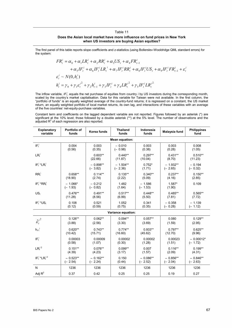
BIS Papers No 2 67
Table 11Does the Asian local market have more influence on fund prices in New York
when US investors are buying Asian equities?
The first panel of this table reports slope coefficients and z-statistics (using Bollerslev-Wooldridge QML standard errors) forthe system:
25
24312
210
198765
143210
),0(~it
it
it
it
it
it
it
it
it
it
it
itt
it
it
it
it
it
it
itt
it
it
it
LRIFLRIFhh
hNFRIFUSIFRRIFLRIFIF
FRUSRRLRFR
The inflow variable, IFti, equals the net purchase of equities from country i by US investors during the corresponding month,
scaled by the countrys market capitalisation. Data for this variable for Taiwan were not available. In the first column, theportfolio of funds is an equally weighted average of the country-fund returns; it is regressed on a constant, the US marketreturn, an equally weighted portfolio of local market returns, its own lag, and interactions of these variables with an averageof the five countries net-equity-purchase variables.
Constant term and coefficients on the lagged dependent variable are not reported. Figures followed by an asterisk (*) aresignificant at the 10% level; those followed by a double asterisk (**) at the 5% level. The number of observations and theadjusted R2 of each regression are also reported.
Explanatoryvariable
Portfolio offunds Korea funds Thailand
fundsIndonesia
funds Malaysia fund Philippinesfund
Mean equation:
IFti 0.004 0.003 0.010 0.003 0.003 0.008
(0.56) (0.35) ( 0.98) (0.38) (0.28) (1.05)
LRti 0.603** 0.440** 0.297** 0.431** 0.510**
(22.66) (11.87) (10.04) (8.70) (11.23)
IFti *LRt
i 0.898** 1.504** 0.752* 1.932** 0.194( 3.82) ( 2.36) (1.71) ( 2.65) ( 0.32)
RRti 0.658** 0.114** 0.135** 0.340** 0.237** 0.150**
(18.90) (2.74) (2.22) (5.09) (4.16) (2.85)
IFti *RRt
i 1.066* 0.212 1.482 1.586 1.587* 0.109( 1.93) ( 0.82) (1.64) ( 1.53) (1.90)
USt 0.476** 0.491** 0.517** 0.448** 0.485** 0.565**(11.28) (8.56) (6.99) (5.50) (7.81) (7.72)
IFti *USt 0.108 0.521 1.052 0.341 0.358 1.139
(0.12) (0.59) (0.75) (0.35) ( 0.28) ( 1.12)
Variance equation:
0.126** 0.062** 0.094** 0.057** 0.080 0.129**2 it (3.88) (2.56) (3.30) (3.69) (1.59) (2.95)
ht-1i 0.620** 0.743** 0.774** 0.933** 0.797** 0.625**
(10.42) (15.71) (16.60) (45.62) (12.70) (9.96)
IFti 0.00003 0.00009 0.00002 0.00002 0.00023 0.00012*
(0.58) (1.07) (0.30) (1.28) (1.51) ( 1.72)
LRti 2 0.151** 0.076** 0.099** 0.007 0.116** 0.199**
(4.39) (4.23) (3.17) (1.57) (2.09) (4.31)
IFti *LRt
i 2 0.523** 0.162** 0.150 0.086** 0.856** 0.846**( 2.54) ( 2.24) (0.44) ( 2.52) ( 2.04) ( 2.63)
N 1236 1236 1236 1236 1236 1236
Adj R2 0.37 0.42 0.25 0.25 0.19 0.27
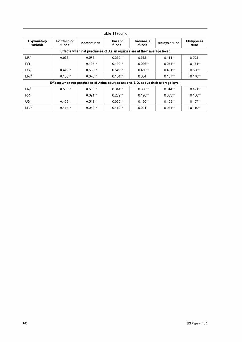
68 BIS Papers No 2
Table 11 (contd)
Explanatoryvariable
Portfolio offunds Korea funds Thailand
fundsIndonesia
funds Malaysia fund Philippinesfund
Effects when net purchases of Asian equities are at their average level:
LRtI 0.628** 0.573** 0.395** 0.322** 0.411** 0.503**
RRtI 0.107** 0.180** 0.286** 0.254** 0.154**
USt 0.479** 0.508** 0.549** 0.460** 0.481** 0.526**
LRti 2 0.136** 0.070** 0.104** 0.004 0.107** 0.170**
Effects when net purchases of Asian equities are one S.D. above their average level:
LRtI 0.583** 0.503** 0.314** 0.368** 0.314** 0.491**
RRtI 0.091** 0.259** 0.190** 0.333** 0.160**
USt 0.483** 0.549** 0.605** 0.480** 0.463** 0.457**
LRti 2 0.114** 0.058** 0.112** 0.001 0.064** 0.119**
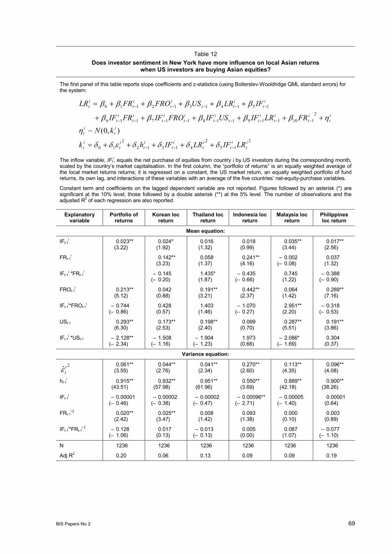
BIS Papers No 2 69
Table 12Does investor sentiment in New York have more influence on local Asian returns
when US investors are buying Asian equities?
The first panel of this table reports slope coefficients and z-statistics (using Bollerslev-Wooldridge QML standard errors) forthe system:
215
241312
210
2110119118117116
15141312110
),0(~it
it
it
it
it
it
it
it
it
it
it
it
itt
it
it
it
it
it
it
itt
it
it
it
LRIFLRIFhk
kNFRLRIFUSIFFROIFFRIF
IFLRUSFROFRLR
The inflow variable, IFti, equals the net purchase of equities from country i by US investors during the corresponding month,
scaled by the countrys market capitalisation. In the first column, the portfolio of returns is an equally weighted average ofthe local market returns returns; it is regressed on a constant, the US market return, an equally weighted portfolio of fundreturns, its own lag, and interactions of these variables with an average of the five countries net-equity-purchase variables.
Constant term and coefficients on the lagged dependent variable are not reported. Figures followed by an asterisk (*) aresignificant at the 10% level; those followed by a double asterisk (**) at the 5% level. The number of observations and theadjusted R2 of each regression are also reported.
Explanatoryvariable
Portfolio ofreturns
Korean locreturn
Thailand locreturn
Indonesia locreturn
Malaysia locreturn
Philippinesloc return
Mean equation:
IFt-1i 0.023** 0.024* 0.016 0.018 0.035** 0.017**
(3.22) (1.92) (1.32) (0.99) (3.44) (2.56)
FRt-1i 0.142** 0.058 0.241** 0.002 0.037
(3.23) (1.37) (4.16) ( 0.08) (1.32)
IFt-1i *FRt-1
i 0.145 1.435* 0.435 0.745 0.388( 0.20) (1.87) ( 0.66) (1.22) ( 0.90)
FROt-1i 0.213** 0.042 0.191** 0.442** 0.064 0.289**
(5.12) (0.88) (3.21) (2.37) (1.42) (7.16)
IFt-1i*FROt-1
i 0.744 0.428 1.403 1.070 2.951** 0.318( 0.86) (0.57) (1.46) ( 0.27) (2.20) ( 0.53)
USt-1 0.293** 0.173** 0.198** 0.099 0.287** 0.191**(6.30) (2.53) (2.40) (0.70) (5.51) (3.86)
IFt-1i *USt-1 2.128** 1.508 1.904 1.973 2.086* 0.304
( 2.34) ( 1.16) ( 1.23) (0.66) ( 1.69) (0.37)
Variance equation:
0.061** 0.044** 0.041** 0.270** 0.113** 0.096**2 it (3.55) (2.76) (2.34) (2.60) (4.35) (4.08)
ht-1i 0.915** 0.932** 0.951** 0.550** 0.889** 0.900**
(43.51) (57.98) (61.96) (3.69) (42.18) (38.26)
IFt-1i 0.00001 0.00002 0.00002 0.00096** 0.00005 0.00001
( 0.46) ( 0.38) ( 0.47) ( 2.71) ( 1.40) (0.64)
FRt-1i 2 0.020** 0.025** 0.008 0.093 0.000 0.003
(2.42) (3.47) (1.42) (1.38) (0.10) (0.89)
IFt-1i*FRt-1
i 2 0.128 0.017 0.013 0.005 0.087 0.077( 1.06) (0.13) ( 0.13) (0.00) (1.07) ( 1.10)
N 1236 1236 1236 1236 1236 1236
Adj R2 0.20 0.06 0.13 0.09 0.09 0.19
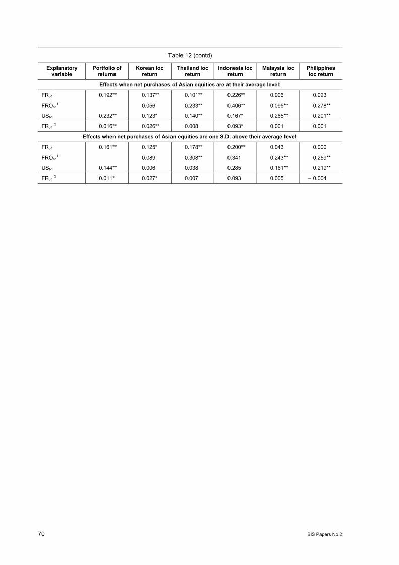
70 BIS Papers No 2
Table 12 (contd)
Explanatoryvariable
Portfolio ofreturns
Korean locreturn
Thailand locreturn
Indonesia locreturn
Malaysia locreturn
Philippinesloc return
Effects when net purchases of Asian equities are at their average level:
FRt-1i 0.192** 0.137** 0.101** 0.226** 0.006 0.023
FROt-1i 0.056 0.233** 0.406** 0.095** 0.278**
USt-1 0.232** 0.123* 0.140** 0.167* 0.265** 0.201**
FRt-1i 2 0.016** 0.026** 0.008 0.093* 0.001 0.001
Effects when net purchases of Asian equities are one S.D. above their average level:
FRt-1i 0.161** 0.125* 0.178** 0.200** 0.043 0.000
FROt-1i 0.089 0.308** 0.341 0.243** 0.259**
USt-1 0.144** 0.006 0.038 0.285 0.161** 0.219**
FRt-1i 2 0.011* 0.027* 0.007 0.093 0.005 0.004

BIS Papers No 2 71
Comments on Information flows during theAsian crisis: evidence from closed-end funds
by Benjamin H Cohen and Eli M RemolonaTatsuya Yonetani, Bank of Japan
I am very pleased to be here today and to comment on this very interesting and constructive paperdealing with information flows during the international financial crisis. In my view, the Cohen andRemolona paper is an excellent example of the insights empirical research gives practitioners andpolicy makers into policy questions regarding market design and regulations. Specifically, the paperexamines global flows of information before, during and after the Asian crisis and offers importantinsights into the debate over the cause of the financial crisis and activities of foreign investors such ashedge funds. I will not go into the content of the paper in detail, but would like to point out some of themost interesting findings.
First, the paper focuses on the direction of information flows with respect to financial market returns inAsian markets; did information flow from the domestic markets to the US market, or vice versa?
As the paper points out, this question is a fundamental one in understanding the Asian financial crisisbecause, depending on the answer, different lessons could be derived from the experience regardingthe cause of the financial crisis.
The finding of the paper in this respect is that while information flows between local and US marketstended to be roughly evenly balanced before the crisis, US market returns assumed a more importantrole during the crisis. The paper also finds that the shift in causation between the US and Asiareflected US market sentiment playing a greater role than the news that became known during UStrading hours.
These findings are very interesting and I am interested to know what exactly they mean. The authorsconclude that they reflected changes in investor sentiment, but what transmission mechanisms can beidentified and through which changes does US investor sentiment have a material effect indetermining emerging-market returns?
In my view, there seem to be several explanations to the mechanisms. One explanation emphasizesinformation linkage. Connections between US closed-fund returns and local market returns occurthrough information. If both markets share some common factor regarding risk and return, then fundreturns in one market have an impact on those in the other market. In this explanation, the marketdoesnt need to be connected with other markets in a transactional sense. A shock may be transmittedfrom the US market to Asian markets, even though investors trading in the former might be completelydifferent from those in the latter. The only thing needed is some shared some common factorregarding risk and return.
Regarding information linkage, the paper provides us with a very interesting insight, namely that thecommon factor reflected US investors sentiment toward specific markets, and not merely the newswhich was known during US trading hours. This seems to imply that global contagion spreads fromindustrial countries to emerging economies only when investors recognize events or news asimportant factors to be considered in specific risk-return relationships.
An alternative explanation to the mechanisms producing contagion and amplifying market dynamicscould be the effect of portfolio rebalancing. From this point of view, contagion occurs through tradingfor portfolio rebalancing purposes. A typical example is the repatriation of funds from emergingmarkets by investors in industrial countries. Actually, it is said that some signs of such behaviour wereobserved in some Asian countries in the first half of this year, which was affected by US stock marketcorrections. Such behaviour can perhaps, to some extent, be explained by the decreasing willingnessof investors to shoulder credit risk because of losses incurred by US stock market corrections.
In this context, findings in the paper might be interpreted as follows: Investors rebalanced theirportfolios because returns in other markets had a direct effect on their risk tolerance. Movements inUS markets had such an effect on US-based closed-fund investors, but not so on local marketinvestors. Stronger interconnection between US-based closed-funds and local funds during the crisismight suggest the existence of international investors who invested in both US-based closed-fundsand local funds. I think such a supposition is plausible, because such investment in different types of

72 BIS Papers No 2
funds, in which the underlying instrument is the same but liquidity is different, could contribute tohedging or arbitraging purposes.
Supposing that a shock was strongly transmitted between the US market and Asian markets throughinformation linkage or through rebalancing effects during the crisis, why was the direction ofinformation flow from US market returns to local markets returns more strongly transmitted and notvice versa? Is it because mature-market investors have better information about emerging marketsthan local market investors? Or is it because US market returns have a bigger effect on the risktolerance of international investors than local market returns? I think this is a very interesting questionon which future research in this area might focus.
Another interesting finding in the Cohen and Remolona paper concerns market sentiment and capitalflows between the US and Asian markets. The paper suggests US investors tended to be contrariansin their portfolio activities vis-à-vis Asia: they purchased Asian equities just when their opinions differedmost from investors in the local markets.
As I see it, this finding is actually confirmed by trends in US capital flow data and is very stimulating inunderstanding the market dynamics during the crisis. According to capital movement statistics by theUS Treasury Department as shown in Chart 1, US investors seemed to purchase Asian stocks at lowprices even during the Asian crisis and sold them at higher prices to take profits in the latter half of1999.
In contrast, Japanese investors exhibited different investment behaviour, as shown in Chart 2. It wasnot until 1999 that net equity investment from Japan to Asian countries turned to a positive figure.These results might suggest that not only local investors but also Japanese investors pursued positivefeedback strategies toward Asian equities during the crisis, while US investors followed negativefeedback strategies.
What accounts for such a difference between the two types of investors?
Does this mean that Asian investors, including Japanese investors, were so greatly affected by localnews that they could not make objective judgement about investment in Asian equities? Or does thisdifference stem from that of different time horizons? This point is interesting and could be related tothe issue regarding information asymmetry between US investors and local investors.
In my view, the debate over investor strategies as to whether positive feedback or negative feedbackand the impact on the market is particularly important, in the sense that it could be a key aspect ofmarket dynamics during the crisis. If positive feedback investors become dominant in the market whenmarket strains emerge, they tend to close out their long positions even though there may be strongsuspicion that prices have overshot only temporarily. Such herding behaviour exacerbates marketpressures. Typically, it is said that such a mechanism occurred in autumn 1998. However, the papersuggests that US-based international investors should perhaps not always be regarded as the culpritsof the Asian crisis, whose sharp outflow of portfolio investments brought about declines in assetprices. In fact, they could even be regarded as having helped market prices recover in the healingprocess after the crisis.
It is said that recently index-based investment style has become more prevalent and having more ofan impact on the market. Such investors are typical positive feedback ones and I think the analyticalframework in the paper may be applied to analyse such changes in investment style in the market.
In closing, once again I would like to say that many of the findings in the paper contain stimulatingpoints which should be taken into account when considering policy issues regarding market designand regulations. I hope such empirical studies as these will further contribute to such policy issues inthe future.
Thank you for your kind attention.
BIS Papers No 2 73
Comments on Information flows during theAsian crisis: evidence from closed-end funds
by Benjamin H Cohen and Eli M RemolonaTorben G Andersen
Northwestern University andNational Bureau of Economic Research
The recent Asian crisis has generated a heated debate regarding the underlying causes and theappropriate policy response. Cohen and Remolona provide a very nice and succinct summary of theliterature, outlining opposing positions classifying the crisis as either home grown or driven bydevelopments in international financial markets. In the course of weighing the evidence they reviewrelevant data on the direction of foreign capital flows and the premia on US closed-end Asian equityfunds. Although such data is useful, they note it has inherent limitations. In particular, it is at bestavailable at a weekly interval rendering direct analysis of the dynamics of the information flow duringthe crisis impossible. Being able to study the markets at a daily frequency and investigating whetherreturn relevant information has its origin in Asia and is flowing from Asia to foreign markets or viceversa is of interest for a number of reasons. It permits a more direct examination of the dynamics ofthe crisis and the role exerted by different factors. For example, it may shed light on whether foreign"speculators" were to blame for the development and what may be achieved by imposing restrictionson international capital flows. It would thus also speak indirectly to the desirability of including privateinvestors in debt workouts and the appropriate role of IMF.
Unfortunately, data that allow us to explore this issue directly is not readily available since the stocksAsian equities typically are not traded outside of the local markets. Cohen and Remolona suggest aninteresting way around this problem. They analyse the daily interaction between returns on local Asianequity markets and US closed-end funds investing in these Asian equity markets. Although the netasset value of the stocks underlying the fund is not available daily, the market price of the fund is.Comparing the associated daily fund returns with the daily Asian equity-index returns provides directevidence on the relative valuation of these assets from a US versus a local perspective.
The above observation motivates the regression-based analysis in the remainder of their paper. Thecomments below focus on methodological aspect of their approach. My main concern is that theexplored regressions are hard to interpret and fail to fully exploit the lack of overlap between thetrading in the local Asian and the US market. To illustrate my point it is convenient to consider astylised framework. Assume first that the portfolio of stocks underlying the US traded closed-end fundis identical to the basket making up the local Asian equity index so that the returns are based on thesame underlying assets, and investors may purchase the fund and stock index freely at no transactioncosts. Second, assume that the returns are uncorrelated and the expected daily mean returns aresmall relative to the return innovations. These characteristics are broadly consistent with thehypothesis of an efficient market, although we may anticipate positive autocorrelation in the indexreturns due to nonsynchroneous trading effects. However, one may readily control for such features inpractice. Third, let the calendar day be split into two consecutive segments, the Asian trading dayfollowed by the US trading day. For simplicity, we assume no overlap and no separation between thetwo trading periods. Consequently, the close-to-close (CC) fund return, Rt
F(CC), is composed of twodistinct uncorrelated return innovations, t
F and tL. Likewise, the close-to-close local return, Rt
L(CC),consists of two uncorrelated components, t
L and t-1F. In contrast, note that the corresponding open-
to-close (OC) returns are RtF(OC) = t
F and RtL(OC) = t
L. We also stipulate constant returnvariances, Var( t
F ) = F2 and Var( t
L ) = L2.
A stylised representation of the Cohen and Remolona regressions take the form,
RtF(CC) = a0 + a1 Rt
L(CC) + utF, (1)
and
RtL(CC) = b0 + b1 Rt-1
F(CC) + utL, (2)
Exploiting the decomposition of the close-to-close returns, we may rewrite (1) as
tL = a0 + a1 ( t
L + t-1F ) + ( ut
F - tF ), (3)
where the "error" term, utF - t
F , is uncorrelated with the "regressor," tL + t-1
F , while the dependentvariable, t
L , is identical to one component of the regressor and orthogonal to the other, t-1F .

74 BIS Papers No 2
Consequently, equation (1) may be interpreted as an "error-in-variables" regression, where theopen-to-close local Asian index return is regressed upon a noisy version of itself. If the secondcomponent was not included in the regressor, we would trivially have an asymptotic regressioncoefficient of unity, i.e., plim a1 = 1. Given the "error-in-variables" representation, standard resultsinstead imply,
plim a1 = 1 - [ F2 / ( L
2 + F2 ) ]. (4)
Equation (4) constrains a1 to the unit interval. Moreover, a1 increases with the size of the returninnovations during local Asian trading relative to US trading. This suggests a simple interpretation ofshifts in a1 across subsamples: A declining a1 implies that relatively more return relevant information isgenerated during US trading hours and vice versa. Similar arguments apply to equation (2). We have,
plim b1 = 1 - [ L2 / ( F
2 + L2 ) ]. (5)
Within this stylised setting, we thus have plim ( a1 + b1 ) = 1, which reinforces the interpretation of thecoefficients as representing shares of return relevant information generated in the respective tradinghours. These findings suggest the following interpretation of the evidence in the paper. First, thecoefficients corresponding to a1 are almost universally higher than those corresponding to b1, implyingthat the local Asian business hours generate the majority of the return relevant information for theAsian stocks. The higher regression R2 of the specifications corresponding to equation (1) relative to(2) (Table 5 versus Table 6 in the paper) is also consistent with this view. Second, the drop in a1 andincrease in b1 during the crisis period point to a relative elevation in the role of the US market segmentduring the crisis itself. These findings support the discussion in the paper.
Unfortunately, the formal justification behind these interpretations break down in the representationswhere additional variables, correlated with the above return innovations, are introduced into thesystem. Because the specifications include indicators observed simultaneously with both the localreturn (regional Asian market returns) and fund returns (US market index), the interpretation isconfounded by complicated and likely time-varying correlation effects that are hard to assess within an"error-in-variables" style regression. This is further accentuated if one uses close-to-close returns forthe auxiliary indices as they span both the Asian and US trading periods, and hence generally will becorrelated with both Asian and fund return innovations. In particular, the direct interpretation of therelative size of the coefficients is lost and the estimates no longer cumulate to a meaningful measureof overall significance. Confirming this observation, the coefficients corresponding to a1 and b1aggregate to less than unity -- slightly so in the pre-crisis period but much so during the crisis itself.Rather than trying to decipher the interactions between the parameter estimates in this settingcomplicated by the correlations induced by the overlap between close-to-close returns, I encouragethe authors to explore an alternative set of regressions that avoid the overlap between returncomponents among the regressors and thus are more readily interpretable. The only additionalrequirement is access to daily opening prices as well as closing prices. For example, consider
RtF(CO) = c0 + c1 Rt
L(OC) + c2 RRt(OC) + v1,tF, (6a)
RtF(OC) = d0 + d1 Rt
L(OC) + d2 USt(OC) + v2,tF, (6b)
RtF(CC) = e0 + e1 Rt
L(OC) + e2 Rt-1F(OC) + v3,t
F. (6c)
Notice that equation (6a) relates the fund return to the local Asian return over the period where onlythe Asian markets are trading. Hence, it checks whether the fund opening price incorporates the returninnovation from the Asian market one-for-one (c1 = 1). Some discrepancy may also be found if theassets held by the fund differ systematically from those in the local market index. As such, this servesas a useful control. In addition, one may gauge whether the other regional Asian stock indices impactthe pricing of the fund beyond the effect already reflected in the local market (c2 0). Equation (6b)studies whether there is a delayed reaction or systematic spill-over in sentiment from Asia to UStrading in Asian stocks (d1 0). Here, I have also included the contemporaneous US return to checkfor a direct relation between the US market and the valuation of the local Asian assets. Finally,equation (6c) relates the close-to-close fund return to the local Asian open-to-close return, where wemay test e1 = 1 without worrying about an error-in-variables problem. For illustration, I have alsoincluded the lagged fund return to control for autocorrelation due to nonsynchroneous trading, e2 = 0.This type of specification is much easier to deal with econometrically, and the associated interpretationof the estimates is more straightforward. Furthermore, modifications of equation (6a-c) that focus onalternative variables or controls are readily constructed.

BIS Papers No 2 75
Cohen and Remolona also study the volatility dynamics of the return series. The spirit of mycomments also applies to this analysis. They base the analysis on close-to-close returns thatpotentially obscure the underlying relationships and certainly render the interpretation of thecoefficients much more difficult than necessary. There is a well-established literature on volatilityspill-overs that carefully calibrate and standardise non-overlapping return and volatility component in amanner that preserve the interpretation of standard volatility persistence measures from the dailyunivariate GARCH literature, rendering both marginal coefficients and cumulative effects meaningful.This is simply not attainable with the complex correlation structures that is induced among the variousreturn components generated by overlapping close-to-close returns. Good illustrations of suchprocedures are provided in Engle, Ito and Lin (1990, Econometrica) and Hamao, Masulis and Ng(1990, Review of Financial Studies).
In conclusion, I find the paper both insightful and stimulating. It provides an excellent introduction tothe crisis debate and points to an interesting set of data that may help us address questions directlyrelated to the key issues. They establish that flight by foreign investors was not the driving force in themarket collapse. The analysis also suggests that the US traded Asian funds were more importantfactors in the return dynamics during the crisis than either before or afterwards, and that the USdomestic market in turn became more critical for the returns on the US based Asian country funds.This points towards an increased importance of the US market sentiment during the crisis. My morecritical comments are motivated by the desire to see the available data exploited to the fullest so thatthe results are further robustified and the parameter estimates rendered more directly interpretable.


BIS Papers No 2 79
Estimating liquidity premia in theSpanish Government securities market1
Francisco Alonso, Roberto Blanco,Ana del Río, Alicia Sanchís, Banco de España
Abstract
This paper investigates the presence of liquidity premia in the relative pricing of assets traded on theSpanish government securities market. Firstly we propose a classification of bonds consisting on fourcategories that identify groups of bonds with a different degree of liquidity. Secondly we estimateliquidity premia, including liquidity parameters in the estimation of the zero-coupon yield curve. Theresults suggest the existence of a significantly higher yield (adjusted for differences in cash flows) fornon-strippable bonds that mostly reflects their lower degree of liquidity. Secondly, post-benchmarkbonds display a positive liquidity premium over benchmark issues. Thirdly, the lack of liquidity of pre-benchmark bonds does not seem to be priced. We also show that these pricing discrepancies arerobust to the impact of taxes on bonds. The size of relative liquidity premia seems relatively small.
1. Introduction
The liquidity of an asset is generally understood as the ease of its conversion into money.2 In practice,the conversion of an asset into money involves certain costs: searching costs, delays, broker’scommissions, etc. The higher these costs the lower the degree of liquidity of the asset. In mostfinancial markets there is a class of agents known as market makers whose function is to provideliquidity. These agents are ready to buy and sell securities up to a maximum amount and make theirprofit on the difference between the bid and ask prices. These latter are the prices at which the othermarket participants can execute surely and immediately sell and buy transactions, respectively. As aconsequence, the bid-ask spread reflects the cost incurred by a typical investor to unwind an assetposition, which is part of the cost of converting an asset into money. This is why the bid-ask spread isone of the most widely used measures of liquidity.
According to market microstructure models, the bid-ask spread may reflect three different costs facedby market-makers: asymmetric information costs, inventory costs, and order processing costs.However, as Gravelle (BIS, 1999) points out, asymmetric information costs should not be verysignificant in the case of government securities (GS). This implies that liquidity in the GS marketsshould be closely linked to the market-makers’ inventory risk and order processing costs whichultimately depend on the level of risk of the asset (duration) and the frequency with which a transactionwill be executed (turnover). Sometimes, liquidity is measured by some indicators of market activity(turnover, turnover ratio, benchmark status, age).
Because investors value asset liquidity we can expect liquidity and differences in liquidity to be priced.In other words, investors may require a liquidity premium for holding illiquid assets in order tocompensate them for bearing higher transaction costs. In the literature, there are some papers thattest for the existence of liquidity premia in securities markets. The bulk of this literature focuses onequity markets,3 whereas there are only a few papers that focus on debt markets, most of them usingUS market data.
1We wish to thank Juan Ayuso, Christian Upper, Oreste Tristani, Clemente Fernández, Alfredo Martínez, VíctorGarcía-Vaquero, Jorge Martínez and participants in the BIS’ Workshop on Market Liquidity for helpful comments andsuggestions.
2See Market liquidity: Research Findings and Selected Policy Implications in BIS (1999) for the various dimensions ofliquidity.
3See, for example Amihud and Mendelson (1986,1989).

80 BIS Papers No 2
Papers that test for the existence of a liquidity premium in the GS markets have followed a number ofapproaches. For example, in Amihud and Mendelson (1991), Kamara (1994) and Garbade (1996) theliquidity premium is only estimated for short-term US Treasuries. They compare the yield of notes withthat of bills with the same term to maturity. Since both instruments are identical, except for the fact thatnotes are more actively traded, yield differences are attributed to differences in liquidity. The liquiditypremia in these papers are found to be high and significant. Elton and Green (1998) use volume as aproxy for liquidity and introduce it as an explanatory variable when fitting a zero-coupon curve to theUS market. They find that the coefficient of this variable is significant for most of the days considered,although the implied liquidity premium is very small. Warga (1992) proxies liquidity by indicatingwhether or not an issue is on-the-run (the most recently issued security of a particular maturity). Hecompares the ex-post monthly excess return over the 30-day Treasury bill rate for two series ofconstant duration portfolios made up of securities traded on the US market, one containing on-the-runbonds and the other containing the other available bonds. Warga (1992) finds that the portfolioshaving the on-the-run bonds exhibit a lower return and interprets this as evidence of a liquiditypremium. In other papers, like Shen and Starr (1998), liquidity is proxied by the bid-ask spread. In thatpaper the term premium, proxied by the excess ex-post returns of the six-month US T-bill over the3-month bill, is estimated and it is found that the bid-ask spread accounts for a substantial portion ofthis premium.
The estimation of liquidity premia in GS markets is important because among other reasons, it mightimprove the information content of prices. For example, the existence of liquidity premia may distortthe information extracted from the estimated term structure or the estimates of implied inflationexpectations obtained by comparing fixed-coupon and inflation linked bonds.
Against this background, the main goal of this paper is to investigate whether there is a liquiditypremium in the relative pricing of assets traded on the Spanish GS market. To do this, we firstcharacterise the relative liquidity of bonds. The strippability of the asset and its benchmark statusappear to be two relevant determinants of securities’ liquidity within each maturity zone. Given thisproperty, we consider four categories of bonds that take into account these elements. The categoriesare non-strippable bonds and pre-benchmark (bonds that will have the benchmark status in thefuture), benchmark and post-benchmark (bonds that had the benchmark status in the past) strippablebonds. We find that there are important liquidity differences among these categories of bondsaccording to different measures of liquidity based on activity measures and bid-ask spread.Benchmark bonds are the most liquid, followed by strippable non-benchmark bonds. And finallynon-strippable bonds appear to be very illiquid.
In the second part of the paper we estimate relative liquidity premia. A traditional approach consists oncalculating yield spread between non-benchmark and benchmark bonds. However, this estimation ofthe liquidity premia do not control for risk and tax factors derived from different cash flow structures ofbonds. Our methodology follows that of Elton and Green (1998) which is based on the estimation ofthe term structure of interest rate. This approach allows us a better control of effects related to thecash flow structure of bonds. Concretely, we incorporate liquidity effects in the estimation ofzero-coupon yield curve introducing dummy variables for the different categories of bonds. The resultssuggest the existence of a significantly higher yield, adjusted for differences in cash flows, for non-strippable bonds that seems to mostly reflect their lower degree of liquidity. Second, post-benchmarkbonds display a positive liquidity premium over benchmark issues. Third, the lack of liquidity ofpre-benchmark bonds does not seem to be priced. Even, in some periods, we find evidence of anegative premium over benchmark issues for pre-benchmark bonds. We also show that these pricingdiscrepancies are robust to the impact of taxes on bonds. Thus, these results point to the existence ofa liquidity premium in the relative pricing of bonds traded on the Spanish GS market, although its sizeseems relatively small.
The remainder of the paper is organised as follows. Section 2 describes the structure of the SpanishGS market. Section 3 describes the data. Section 4 proposes a classification of bonds which tries toidentify bonds with a different degree of liquidity. Section 5 estimates liquidity premia. And, finallySection 6 summarises the main conclusions.
2. Structure of the Spanish government securities market
Two types of instruments are issued by the Spanish Treasury: Letras del Tesoro (Treasury bills),which are short-term securities issued at a discount, and Bonos y Obligaciones del Estado (Statebonds) which are medium and long-term securities with annual coupon payments. Both types of
BIS Papers No 2 81
instruments are represented by book entries and issued via regular competitive auctions. Bills areissued at 6-, 12- and 18-month maturities, whereas bonds are issued at 3-, 5-, 10-, 15- and 30-yearmaturities. Auctions take place on a monthly basis, except for 30-year issues, which are auctionedevery two months, and 12- and 18-month issues, which are auctioned fortnightly. In the case ofmedium and long-term securities issues are reopened over several consecutive auctions until theoutstanding amount reaches a minimum level .The securities allocated at such auctions have identicalnominal coupon and interest payment and redemption dates.
Since July 1997, the Spanish Treasury has been issuing strippable bonds. They enjoy a morefavourable tax treatment for payers of the corporate income tax because the latter are not subject towithholding tax on coupon payments. These securities can be stripped during their life into n+1zero -coupon assets, where n stands for the number of remaining coupon payments, arising from thecash flow generated by the bond’s coupons and principal. The stripping process is conducted by atype of market participant, known as market makers, who assume a number of commitments subjectto annual review. They are also allowed to conduct the reverse process (reconstitution). Alloutstanding bonds issued before July 1997 are non-strippable and do not enjoy the favourable taxtreatment of strippable bonds.
Secondary market trades are conducted through three systems, the first two being reserved for marketmembers, while the third is for transactions between market members and their clients. In the firstsystem (known as a blind market) trading is electronically conducted without knowledge of thecounterparty’s identity. Only those market members who comply with certain requirements andassume a number of commitments can participate in this market segment. For instance, they areobliged to quote during at least 60% of the time of each session the five references of bonds withbenchmark status subject to a maximum bid-ask spread. Blind market trades can only be outrighttransactions, whether spot or forward.
The second trading system (known as second tier) channels all the remaining transactions betweenmarket members. Trading is conducted directly between traders or through brokers. Some brokerspost indicative bid and ask prices on electronic market information systems such as Reuters andBloomberg. In this market segment, participants can trade outright (in spot or forward transactions) orenter into repos. Two types of repo transactions are allowed: ordinary repos and blocked repos, thedifference being the fact that under the second type the buyer cannot transact freely with the securitiespurchased, regardless of the buy-back date set.
Clearing and settlement of GS transactions is carried by the Central de Anotaciones en Cuenta(Book-Entry System). Each market member holds an account in this system. Individuals or institutionswho are not members have to channel transactions through a Managing Institution. The procedureused is one of cash on delivery and transactions are settled three business days later.
In addition to the secondary market, there is a futures and options market (MEFF RF) where theunderlying assets are Spanish GS. At present traded contracts include 5- and 10-year futures andoptions and 30-year futures.
Table 1 provides turnover figures for 1999 for the different market segments and for the different typesof transactions on the Spanish GS market. Repos are the type of transaction with the highest activity,which is mainly concentrated in the very short-term (mainly overnight), followed by outright spotpurchases. By contrast, trading activity through forward, futures, and options transactions, is morelimited.
Table 2 gives a breakdown of the holders of Spanish GS at end-1999. Financial institutions own a verylarge proportion of the outstanding amount (61.2% for bonds and 91.3% for bills). Non-residents alsohave a significant share of the market in the case of bonds (32%). By contrast, the share ofnon-financial companies and households is very low.
3. Data
In this paper we use daily data of prices (quoted and traded), outstanding amounts, and tradingactivity (trading volume and number of trades) for the Spanish GS market from January 1999 to

82 BIS Papers No 2
April 2000. This information is collected for 34 bonds,4 24 of them being outstanding through out thesample period (see Table 3 for a description of the issues). For the short-term, the data refer toTreasury bills and repo transactions.
The price data include the following:
(i) Daily mean prices traded in the blind and second tier markets. This information was providedby the Central de Anotaciones del Banco de España.
(ii) Daily quoted bid and ask prices collected from two sources:
(a) Reuters-BDE: since August 1998 the Banco de España Research Department hasbeen building a database from prices posted by Reuters at 2 p.m. It includes bestquoted bid and ask prices for long and short-term issues; and bid and ask rates forrepo transactions. Bid and ask daily prices are calculated using the quotations of fourbrokers: three5 of them are pre-determined and the fourth is the one who traded mostrecently. From these quotations, the highest bid and the lowest ask prices areselected for each issue. If the bid price is higher than the ask,6 then prices aresequentially removed until a non-negative spread is obtained.
(b) Bloomberg: this agency provides daily quoted prices calculated as the average bidand ask quotations at the close (determined by Bloomberg to be about 5 p.m.). In thiscase, by construction, the bid-ask spread is always positive. Bloomberg also providesbid and ask rates for a wide range of repo transactions.
It is worth noting that these databases of quoted prices use different methodologies to calculate dailybid-ask spreads for each instrument. The Reuters-BDE spread is the best proxy for market spread, butit employs non-contemporaneous quotations that may introduce noise and may bias downwards thesize of the spread. On the other hand, the Bloomberg spread cannot be interpreted as the marketspread, but its main advantage is that it reduces non-contemporaneity problems due to the fact thatquotes are averaged. Both the Reuters-BDE and Bloomberg databases suffer from the shortcomingthat quotations are indicative, not firm, and therefore may not reflect actual prices. This problem arisesfrom the specific microstructure of this market and means that it is desirable to use traded prices ascomplementary information.
Trading activity (number of trades and trading volume) is provided by Central de Anotaciones delBanco de España and refers only to transactions between market members, in both, the blind and thesecond tier market.
4. Classifying bonds by their relative degree of liquidity
4.1. A classification of bonds according to their life cycle and tax treatment
In this section we propose a classification of bonds that tries to identify a number of bonds’ groups witha different degree of liquidity. It is important to stress that the approach we follow in this paper ofclassifying bonds by their relative liquidity is not intended to compare liquidity across different maturityzones but within them. This decision is justified by the methodology we use in the next section toestimate liquidity premia, which consists of fitting a zero-coupon yield curve. With this methodology itwould be very difficult to separate term and liquidity effects if we used a classification of liquidityacross different maturities.
Our classification takes into account two elements of an issue: its stage of the life cycle and itsstrippability (whether or not the issue is strippable). We consider the stage of the life because, ingeneral, trading activity and, consequently, liquidity is related to this. It is well-known that in GSmarkets trading activity tends to be concentrated in a small group of securities known as benchmark
4Strips are not included. The percentage of stripped bonds is very low in the Spanish market.
5Four in the case of short-term instruments.
6In the information provided by Reuters it is not uncommon to find negative bid-ask spreads, possibly due to the lack ofcontemporaneity in quotations.

BIS Papers No 2 83
issues. The prices of these instruments are used for extracting information for macroeconomicanalysis and pricing purposes. In the Spanish GS market there are five benchmark issuescorresponding to 3-, 5-, 10-, 15- and 30-year maturities. Since all issued bonds become benchmarkissues, the life cycle of bonds consists of three stages. In the first stage, the bond is initially issued andits outstanding volume is relatively small, and henceforth, its trading activity is very low and does nothave benchmark status. Henceforth bonds in this stage will be referred to as pre-benchmark issues.New fungible auctions increase the outstanding amount, and trading activity also increases untilbenchmark status is achieved and the issue becomes the most liquid one for a particular maturity.Finally, in the third stage, the bond is replaced by a new benchmark and its activity begins todecrease. Bonds in this stage will be referred to as post-benchmark issues.
More specifically, our classification consists on four categories, namely: pre-benchmark, benchmark,post-benchmark and non-strippable issues. The first three categories are only made up of strippablebonds, whereas the last category includes all non-strippable bonds. We have decided to group allnon-strippable bonds in one specific category for the following two reasons. Firstly, in our sample, allnon-strippable bonds are at a very advanced third stage of their life cycle, therefore they are veryilliquid. And, secondly they are subject to a less favourable tax treatment that could be reflected in atax premium.
Over our sample period there was no official classification of benchmark issues in Spain. As aconsequence, the identification of the benchmark issue may be difficult during transition periods. Thecriterion we use in this paper considers that a new bond becomes the benchmark issue when it hasbeen traded more than the old benchmark for at least three consecutive days. Table 4 gives the dateson which a benchmark bond changes according to this criterion, and compares them with thosereported by Reuters and Bloomberg. It can be observed that dates do not coincide for the differentcriteria, but differences between them rarely exceed one month.
Figure 1 shows the life cycle for all the strippable 10-year bonds of our sample. Over this period tworeplacements take place, one in February 1999 when the 5.15% bond becomes the new benchmark.The other takes place in October 1999, where the most recently issued bond (4% with maturity at31/1/10) acquires the benchmark status. This figure displays the evolution of trading activity,outstanding volume and bid-ask spread. It can be seen that the life cycle in trading activity appearsalso to be incorporated in the evolution of bid-ask spreads, suggesting a very different degree ofliquidity of bonds depending on the stage of life they are at.
Table 5 gives a descriptive analysis of previously defined bond categories over our sample period. Itcan be seen that benchmark issues account, on average, for almost 53% of the daily trading volume(see panel c). Regarding non-strippable bonds, despite the high number of issues (20 issues at thebeginning of the period and 16 at the end), they account for just 7% of daily trading volume (seepanel c). Finally, the remaining 40% of the trading volume corresponds to strippable non-benchmarkbonds - of which pre-benchmark issues account for a 15% and post-benchmark issues for a 25%.There are 4 such bonds at the beginning of the period increasing to 9 by April 2000.
Looking at trading activity by maturity, a high concentration around the 10-year zone is observed, withapproximately 33% of the total market activity. The 3- and 5-year maturities account for approximately25% and 23% respectively. And finally, the zones of 15- and 30-year residual maturity have the lowestactivity, with approximately 5% and 3% of total market activity respectively.
Regarding outstanding volume, panel b of Table 5 shows a very different distribution. In particular, ahigh concentration (more than 50%) is observed in the 0-6 years zone.
4.2. Is this classification useful to identify groups of bonds with a different degree ofliquidity?
We now show to what extent the four categories we propose are useful to identify groups of bondswith a different degree of liquidity. To do this we compute some liquidity measures for the differentcategories of bonds.
Table 6 reports various measures of liquidity, all based on trading activity, with a breakdown by bondcategory and maturity. These measures are the number of trades, trading volume and turnover ratio.All these indicators are computed per bond and, therefore, can be interpreted as liquidity measures. Afeature shared by all the liquidity measures of Table 6 is the remarkable differences in liquiditybetween the various categories considered.

84 BIS Papers No 2
When comparing liquidity within each maturity zone benchmark issues are the bonds with the greatestliquidity, followed by strippable non-benchmark bonds (for both pre-benchmark7 and post-benchmark).Finally, non-strippable bonds are notable for their very scarce trading activity.
When comparing liquidity among maturity zones the most liquid bonds are those with a residualmaturity between 3 and 10 years. In this regard, it is worth noting that strippable non-benchmarkbonds are sometimes even more liquid than 15 and 30-year benchmark issues.
Figure 2 displays the bid-ask spread8 as a function of the duration for the different categories of bonds.This indicator is used as an additional measure of liquidity. A similar pattern to that reported for tradingactivity also appears here when comparing the liquidity of bonds within each maturity zone (proxied byduration), although now pre-benchmark issues appear to be more similar, in terms of liquidity, tonon-strippable bonds than to post-benchmark strippable issues.
However, note that trading activity and the bid-ask spread would provide a very different ranking ofbonds by liquidity if we did not control for time to maturity or duration. As Figure 2 illustrates, thebid-ask spread is positively correlated with time to maturity. This effect clearly dominates thepreviously reported pattern (benchmark status of the bond). This relationship between spread and timeto maturity, which has also been identified in other GS markets,9 can theoretically be explained by themarket-makers’ inventory risk and order processing costs which ultimately depend on the level of riskof the asset proxied by time to maturity. Accordingly, a ranking of bonds using the bid-ask spreadwould classify short-term securities as the most liquid and long-term issues as relatively illiquid.Conversely, a ranking of bonds by the liquidity measures of Table 6 would classify the 10-year bondsas the most liquid issues.
It is worth noting that our classification of bonds can be justified either by the bid-ask spread or by thetrading activity measures because, as was mentioned before, we do not intend to compare liquidityacross different maturity zones but within them.
Three conclusions may be drawn from the previous analysis. Firstly, the benchmark status andstrippability of bonds are two relevant determinants of the liquidity differences within a maturity zonefor the bonds in our sample. Secondly, the four categories we consider seem useful to identify groupsof bonds with a different degree of liquidity. And, finally there seems to be strong differences in liquiditybetween bonds, so that it makes sense to test for the existence of a liquidity premium. This is the aimof the next section of the paper.
5. Estimating liquidity premia
5.1 Preliminary analysis
Our aim in this second part of the paper is to find out if differences in liquidity are priced in the SpanishGS market. One simple approach is to approximate the liquidity premium by the yield spread betweennon-benchmark and benchmark bonds. Applying this measure to the 3,5, 10 and 15-year bonds of oursample always gives a negative figure suggesting the existence of negative liquidity premia. However,it has to be taken into account that some factors may bias this measure. Differences in couponsbetween bonds imply different risk and tax burdens that may make the investor to demand differentyields to maturity for other reasons not related to liquidity effects. The main difficulty when identifyingthe liquidity premium is the separation of the factors explaining differences in yields to maturity. Withthis in mind, our proposal is based on the estimation of the term structure of interest rate, because thisallows us to control any effect associated with differences in maturity and cash flows. This approach issimilar to that followed by Elton and Green (1998).
7Although in the case of the turnover ratio no significant differences are observed between pre-benchmark and benchmarkissues.
8For this analysis we use Reuters-BDE database because it provides a spread measure more closely linked to the concept ofmarket spread (see Section 3 for a description of this database and a comparison with the Bloomberg data).
9BIS (1999) compares bid-ask spreads for “on-the-run” and “off-the-run” issues for Canada, Italy, Japan, UK and US. In allcases they find the same results as ours, except for Japan, where the liquidity of on-the-run 10-year bonds makes theirspread narrower than the one for “on-the-run” 5-year bonds. (See Table 3 of the document Market Liquidity: ResearchFindings and Selected Policy Implications)

BIS Papers No 2 85
According to the analysis developed in Section 4, we distinguish four types of bonds in relation to theirlife cycle and tax-treatment: non-strippable bonds, pre-benchmark, post-benchmark, and benchmarkstrippable bonds.
As a preliminary analysis of the existence of liquidity premia we estimate a zero-coupon yield curveusing the Svensson model10 and analyse yield errors for bonds. We find a very interesting pattern.Figure 3 shows the estimation for a representative day of the sample, (29/3/99) and Table 7 reportsaverage yield errors for each bond in our sample distinguishing its classification over the sample. Thefirst thing we observe is that most non-strippable bonds appear to have on average positive yielderrors, i.e. they are located above the estimated yield curve. The second point to be stressed is thetendency of pre-benchmark bonds to exhibit a lower yield error than benchmark bonds. Finally, theyield error of post-benchmark bonds lies between yield errors of benchmark and non-strippable bonds.These results suggest a preliminary evidence of a positive premium for post-benchmark andnon-strippable bonds over benchmark issues. Next section tries to estimate them using a more formalapproach.
5.2 Estimating the yield curve incorporating liquidity effects
Previous results indicate that the estimation of the yield curve for the Spanish GS market may beimproved if we introduce liquidity and withholding tax affects. Our proposal consists of estimating theterm structure of interest rates using the Svensson model, and introducing additional parameters tocapture these effects. Elton and Green (1998) follow a similar procedure11 introducing volume as ameasure of liquidity. Given that the relationship between traded volume and liquidity may not be linear,we prefer using dummy variables to classify securities according to their degree of liquidity and taxtreatment.
The instantaneous forward rate of term m is modelled in the following way:
NONSTRIPPOSTBENCHPREBENCHem
em
e
mmm
m 2102
31
210211 γγγ
τβ
τβββϕ τττ ++++++=
−−−
where PREBENCH, POSTBENCH and NONSTRIP are dummy variables which take value 1 respectivelyfor pre-benchmark, post-benchmark and non-strippable bonds. Parameters for dummy variables mustbe interpreted in relation to the remaining instruments (3, 5, 10, 15 and 30-year benchmark bonds andshort-run securities).
Parameters 0γ , 1γ and 2γ capture the excess yield demanded on pre-benchmark, post-benchmark
and non-strippable bonds respectively. Parameters 0γ and 1γ can be directly interpreted as liquidity
premia since the tax treatment is the same for all strippable issues. Conversely, parameter 2γ mayincorporate a tax premium in addition to a liquidity premium due to the relatively less favourable taxtreatment of non-strippable bonds. The interpretation of remaining parameters is the standard in theSvensson model.
Once we have modelled the instantaneous forward rate including withholding tax and liquidity effects,we estimate the parameter vector ),,,,,,,,( 210231210 γγγτβτββββ = for each day t as
∑=
−=N
i ti
titi
ppp
1
2)(
minargˆ ββ
where tip is the actual price of bond i at time t and N is the number of securities considered in the
estimation. And )(βtip is the theoretical price obtained from previous specification of the
10See Annex 1 for a description of this model. We use the mid-point between the bid and ask price provided by Bloombergdatabase. Bonds with a remaining life of under a year are excluded from the estimation. For short-term we use repo and billrates.
11They use non-linear least squares to fit a cubic spline to the after-tax cash flows of bonds.
86 BIS Papers No 2
instantaneous forward rate. We minimise price errors instead of yield errors to obtain a better fit for thematurities we are most interested in, i.e. medium and long-term.
We distinguish four nested models. The basic model, called Model 1, does not consider any liquidity ortax effects, i.e. 0γ , 1γ and 2γ are restricted to zero. In Model 2 all these parameters are freelyestimated. Model 3 eliminates the dummy variable for pre-benchmark bonds. And finally, Model 4estimates freely the parameter of the dummy variable for non-strippable bonds, and restricts to zerothe parameters of other dummy variables.
We estimate these four models for the whole sample, from January 1999 to April 2000. Over theperiod 4/1/99 to 30/9/99 the Svensson model does not improve on the Nelson-Siegel model12 andconsequently, we estimate the latter model for this period. Table 813 reports a descriptive analysis ofthe estimated parameters for dummy variables, the root mean square error (RMSE), and the reductionin the RMSE with respect to the basic model.
When all the three dummy parameters are freely estimated (Model 2) the average RMSE is 63% lessthan that of the basic model. The estimated parameter for the non-strippable bonds dummy is positiveand significant for almost the whole sample, indicating that these bonds incorporate a premium overthe benchmark issues that ranges from 2 to 10 basis points in our sample. On average, the excessyield demanded on these bonds is 7 basis points.
Regarding post-benchmark bonds, they also appear to incorporate a premium. It takes the value of5 basis points on average, but in this case there are some periods where the parameter of thisvariable is not positive and statistically significant. Figure 4 shows the evolution of estimatedparameters, 210 ,, γγγ . Shaded areas indicate that 2γ is not statistically significant. These areascoincide with transition periods in benchmark bonds. During January-February 1999 it occurs achange in 3, 5 and 10-year benchmark bonds. During October-December 1999 there is a change of allbenchmark bonds except for 30-year term. Replacements take place gradually in the markets andduring these transition periods frontiers between strippable categories are blurred given the smallnumber of bonds in each one. The approach we follow changes the category of a bond in a specificdate (see table 4) generating sharp movements in the estimations of premium parameters. Thesensitivity of our estimations to benchmark changes does not allow interpreting the evolution of theparameters during transition periods. In any case, results when the categories of bonds are enoughdifferentiated show that post-benchmark bonds include a liquidity premium over benchmark issues.
Regarding the parameter of pre-benchmark bonds, it turns out to be negative on average, suggestingthe existence of a negative premium for these bonds over benchmark issues. However, some caremust be taken in the interpretation of this parameter. It is negatively significant just for 54% of thesample, and for some periods there is just one bond included in this category. The conclusion drawnfrom the analysis of this parameter is that pre-benchmark bonds do not seem to include any positiveliquidity premium in spite of its low liquidity in terms of trading activity and bid-ask spreads. This resultmay possibly be explained by the forward-looking behaviour of investors. It is costly to trade with thesesecurities, but investors do not demand a higher yield because, in the future, these costs will be muchlower when the bond acquires benchmark status. In addition, the limited supply of these issues maycontribute to sustain its price.
Given that pre-benchmark bonds do not appear to have a positive liquidity premium over benchmarkissues, and given that there are not many pre-benchmark bonds in our sample we proceed to grouppre-benchmark and benchmark bonds into the same category. Model 3 includes only two dummyvariables to capture liquidity differences, one for post-benchmark and the other for non-strippablebonds. The reduction of RMSE with respect to the basic model continues to be very high (51%).Non-strippable bonds appear to have a premium of 8 basis points on average, ranging from 5 to12 basis points. This parameter is statistically significant for the whole sample. For post-benchmarkbonds, parameter γ1, is positive and significant for 76% of the sample, showing on average a liquidity
12This model is a particular case of the Svensson model, where the instantaneous forward rate is modelled with just one
hump, i.e. 3β and 2τ are set to zero and one respectively.
13We concentrate on the interpretation of parameters γ0, γ1, γ2, which will be reported in different tables. The remainingparameters of the Svensson and Nelson-Siegel model are presented in Table 12 for all models estimated throughout thepaper.

BIS Papers No 2 87
premium of 5 basis points. Therefore, inclusion of pre-benchmark bonds with benchmark bondsincreases the size of the premia.
Finally, Model 4 includes just one dummy variable for non-strippable bonds. It allows an averagereduction of 37% in the RMSE with respect to the basic model. In this model the average premium fornon-strippable bonds over the remaining bonds is 6 basis points. The size of this parameter is lowerthan in Model 3 because in this case the group of bonds excluded from dummy variables includespost-benchmark issues.
Summing up, the results of this section suggest the existence of a positive liquidity premium forpost-benchmark issues over benchmark bonds, although its size is very small - similar to that found byElton and Green (1998) in the US market. Conversely, the lack of liquidity of pre-benchmark issuesdoes not seem to be priced and, even a negative premium over benchmark issues is found in someperiods. Finally, there is clear evidence of a positive premium for non-strippable bonds in the wholesample. However, as noted before, this premium could not be interpreted directly as a liquiditypremium since the excess yield demanded on non-strippable bonds may also include a withholding taxpremium. In the next section we try to separate these two components.
5.3 Separation of withholding tax and liquidity effects for non-strippable bonds
Previous results show strong evidence of a premium for non-strippable bonds. This premium may bedue to liquidity or withholding tax effects. In order to separate these two elements we re-estimateModel 3 taking into account the withholding tax (Model 5). To do this we modify the cash flows ofnon-strippable bonds in the following way. We reduce the amount of coupon payments by 18%(withholding tax rate during the sample period) and include a new cash flow stream corresponding tothe compensation for the withholding tax. The dates we assign to these cash flows are selected tocoincide with the quarterly tax returns that Spanish corporations are obliged to make. It has to benoted that this procedure considers the maximum cost faced by non-strippable bond holders sincethey can reduce it through coupon washing transactions.14 Consequently, the estimated premium fornon-strippable bonds can be interpreted as a lower bound for the true liquidity premium.
Table 9 reports the estimated parameters, which are comparable with those for Model 3. This modelreduces the premium for non-strippable bonds by only 1.2 basis points, in comparison with Model 3,whereas the premium for post-benchmark bonds does not change significantly. These results suggestthat most of the estimated premia for non-strippable bonds in Models 2 to 4 correspond to liquiditypremia. According to the results of Table 9, the average liquidity premium for non-strippable bonds isat least 6.8 basis points. This minimum liquidity premium for non-strippable bonds is still higher, onaverage terms, than the one found for post-benchmark bonds. This fact is logical given their strongdifferences of liquidity.
5.4 Robustness to tax effects
The above results may be sensitive to including general tax effects in the estimation of thezero-coupon yield curve. That is, they may be affected by the estimation of a pre-tax instead of apost-tax yield curve. It is very difficult to estimate a post-tax yield curve, because tax treatment is verydifferent across investors. In this section we estimate a post-tax yield curve considering the taxtreatment for Spanish corporations, which hold two thirds of the outstanding volume of bonds (seeTable 2).
The theoretical price is expressed as the present value of after-tax cash flows imposing a tax rateof 35% for both interest payment and capital gains. Capital gains or losses at redemption date aredistributed over the life of the bond using a constant yield method, and assuming that the bond is helduntil maturity.
Table 10 shows the main results of the re-estimation of Model 3 using after-tax flows (Model 6). It canbe seen that in this new model the sign and significance of estimated premia remain unchanged, buttheir absolute size is reduced by around 35%. The parameters that capture the asymptotic value of the
14These transactions consist of selling non-strippable bonds to non-resident investors, who are not subject to withholding tax,before the date of the coupon and buying them again after that date.
88 BIS Papers No 2
instantaneous forward rate ( ∞=ϕβ0 ) and the instantaneous forward rate for an infinitely small term to
maturity ( 010 ϕββ =+ ) are also reduced by around 35%. Consequently, the liquidity premiaexpressed as a percentage of these interest rates remain almost unchanged (see Table 11). Theseresults indicate that previously estimated relative liquidity premia are robust to tax effects.
Finally, it is interesting to see that the model with taxes further reduces the RMSE. In average thereduction over the basic model is 77%, which compares with the 51% reduction of the model with twodummies without taxes (model 3). This result suggests the relevance of introducing tax effects whenfitting zero-coupon yield curves.
5.5 Impact of liquidity premia on the estimated yield curve
In this subsection we study the impact of the introduction of liquidity effects on the estimatedzero-coupon yield curve. To do this we compare the estimated parameters for the different models wehave considered in subsections 5.2 to 5.4.
Table 12 reports the mean and the standard deviation of the basic parameters of the term structure.15
The mean of the parameters’ estimates for the models that introduce liquidity effects without taxes(Models 2 to 5) are very close to those of the basic model (Model 1). This is not a surprising resultgiven the relatively small liquidity premia we have found. Conversely, when taxes are introduced(Model 6) some parameters change significantly. β0 and β1 are now around 35% (the tax rate) belowthe estimated level for Model 3, whereas the changes in the other parameters are less dramatic.These changes imply that after-tax zero-coupon rates are around 35% below before-tax rates.
Figure 5 depicts the zero-coupon yield curve at 29/3/99 for two of the models we have estimated,using the Nelson-Siegel approach. The models we consider in this figure are: the basic model(Model 1), and the model that introduces dummy variables for both post-benchmark andnon-strippable bonds (Model 3). The yield curve of the model that accounts for liquidity (Model 3)stands slightly above (with a maximum difference of 9 basis points) that of the basic model forshort-term maturities and slightly below (with a maximum difference of 12 basis points) formedium-term horizons. For long-term maturities both models display very similar rates.
Figure 6 shows the estimated 1-year forward curves implied by the yield curves depicted in Figure 5.Estimated forward rates for horizons shorter than 6 years are slightly lower for the model that accountsfor liquidity effects, whereas the opposite is the case for longer horizons.
Figures 7 and 8 are the same as Figures 5 and 6, except for the fact that they are estimated at 31/3/00using the Svensson model. In this case, the zero-coupon rates are lower for the model that introducesliquidity effects in comparison with the basic model, for all horizons. It is worth noting that for themedium and long-term horizons the difference between the two curves is smaller than that found withFigure 5. This is not surprising given the reduction in the estimated liquidity premia in the second halfof the sample.
The introduction of liquidity effects has allowed us to identify liquidity premia and to reduce the error inthe estimation of the zero-coupon yield curve. However, the implications for information content of theestimated yield curve are not very important. This is an expected result given the small size of theestimated liquidity premium.
5.6 Biases in quoted prices
The results of the previous analysis have been derived from the quoted prices posted by brokers inBloomberg. We know that these prices are not firm, but merely informative and, consequently, we donot know how accurate they are. The existence of a bias in quoted prices may have an impact on theliquidity premia we have estimated. In this subsection we study the existence of biases in quotedprices in comparison with traded prices and derive conclusions on their impact on the estimatedliquidity premia. To do this, for each day and security we compute the difference in yield between themean traded price and the mid-quoted price. Table 13 shows the average of these yield differences for
15From 4/01/99 to 30/9/99 we estimate Nelson-Siegel model, and from 1/10/99 to 14/4/00 Svensson model.
BIS Papers No 2 89
each security, distinguishing its classification along the sample in the four categories we haveconsidered along this paper (pre-benchmark, benchmark, post-benchmark and non-strippable).
Three important features emerge from Table 13. First, average yield differences are very small for allsecurities (between 0 and 2.3 basis points), most of them being not significantly different from zero.Second, yield differences tend to be positive for most bonds (those figures statistically different fromzero are all positive). Third, yield differences tend to be higher for pre-benchmark and non-strippablebonds.
These results suggest the existence of a small negative bias in quoted prices in comparison withtraded prices, which seems to be more important for pre-benchmark and non-strippable issues. Thiswould mean that there is a negative bias in the estimated liquidity premia for non-strippable andpre-benchmark bonds. That is, the actual liquidity premium for non-strippable bonds is higher than theestimated, whereas the absolute value of the liquidity premium for pre-benchmark issues is lower.However, these biases in the liquidity premia should be relatively small given the very small size of thebias in quoted prices. Consequently, the reported results of sections 5.1 to 5.5 seem to be robust tothe data set we have used.
6. Conclusions
The analysis developed in the first part of the paper has showed that there are important liquiditydifferences among securities traded in the Spanish GS market. The strippability of the asset –strippable bonds are the most liquid- and the benchmark status –benchmark bonds are more liquid-appear to be two relevant determinants of the securities’ liquidity within each maturity zone.
The second part of the paper analyses the presence of liquidity premia in the relative pricing of assetstraded in the Spanish GS market. The estimation is carried out introducing liquidity parameters in theSvensson model of the zero-coupon yield curve. These liquidity parameters allow us to estimate theexcess yield of pre-benchmark, post-benchmark and non-strippable bonds over benchmark issues.This methodology improves the traditional approach of the estimation of liquidity premium – whichconsists on computing the yield spread between non-benchmark and benchmark bonds - because itallows an appropriate control of effects associated with differences in maturity and cash flows.
The main conclusions that can be drawn from the estimations made are the following. Firstly, resultssuggest the existence of a positive and significant premium for post-benchmark bonds (both strippableand non-strippable). However, these premia are very small and similar to those found by Elton andGreen (1998) in the US market. Secondly, the lack of liquidity of pre-benchmark bonds does not seemto be priced in the market. Even, in some periods, a negative premium over benchmark issues arisesfor these bonds. This is a somewhat surprising result that can possibly be explained by theforward-looking behaviour of market participants. Thirdly, estimated liquidity premia seem robust to taxeffects and to the data set we have used (quoted prices instead of actual traded prices). Finally,regarding the implications for the estimated zero-coupon yield curve, the introduction of liquidity effectsdo not have significant effects due to small size of the estimated liquidity premia.
References
Amihud, Y. and H. Mendelson (1986) Asset pricing and the bid-ask spread, Journal of FinancialEconomics 17, 223-249.
——— (1989) The effects of beta, bid-ask spread, residual risk and size on stock returns, Journal ofFinance 44, 479-486.
——— (1991) Liquidity, maturity, and the yields on U.S. Treasury securities, Journal of Finance 46,pp. 1411-1425.
Bank for International Settlement (1999) Market Liquidity: Research Findings and Selected PolicyImplications.
Copeland, T.C. and Galai, G. (1983) Information effects on the bid-ask spread Journal of Finance, 38,pp. 1457-1469
Elton, E. J. and T. C. Green (1998) Tax and liquidity effects in pricing government bonds, The Journalof Finance 53, 1533-1562.

90 BIS Papers No 2
Fleming, M. J. and E. M. Remolona (1996) Price formation and liquidity in the U.S. treasuries market:evidence from intraday patterns around announcements, Research Paper 9633, Federal ReserveBank of New York.
Garbade, K. D. (1996) Fixed Income Analysis (MIT Press, Cambridge, Mass.)
Gravelle, T. (1999) Liquidity of the government of Canada Securities Market: stylized facts and somemarket microstructure comparisons to the United States Treasury Market, Bank of Canada, WorkingPaper 99-11.
Kamara, A. (1994) Liquidity, taxes, and short-term Treasury yields, Journal of Financial andQuantitative Analysis 29, 403-417.
Litzenberger, R. H. and J. Rolfo (1984) An international study of tax effects on government bonds, TheJournal of Finance 39, 1-22.
Nelson C. R. and A. F. Siegel (1987) Parsimonious Modelling of yield curves for US Treasury Bills,Journal of Business 60, 473-489.
Núñez, S. (1995) Estimación de la estructura temporal de los tipos de interés en España: elecciónentre métodos alternativos, Banco de España, Documento de Trabajo nº 9522.
Sarig, O. and A. Warga (1989) Bond price data and bond market liquidity, Journal of Financial andQuantitative Analysis 24, 367-378.
Shen, P. and R. M. Starr (1998) Liquidity of the Treasury bill market and the term structure of interestrates, Journal of Economics and Business 50, pp. 401-417.
Svensson, L.E.O. (1994) Estimating and interpreting forward interest rates: Sweden 1992-1994,Centre for Economic Policy Research, Discussion Paper 1051.
Warga, A. (1992) Bond returns, liquidity, and missing data, Journal of Financial and QuantitativeAnalysis 27, 605-617.

BIS Papers No 2 91
Annex
The Svensson model
Svensson (1994) specifies a smooth parametric function for the yield curve. The functional form for theinstantaneous forward rate of term m, mϕ , is the following:
211
23
1210)( τττ
τβ
τββββϕ
mmm
m em
em
e−−−
+++= (A1)
where
),,,,,( 231210 τβτββββ = is the vector of parameters.
m is the term to maturity.
∞=ϕβ0 is the asymptotic value of the instantaneous forward rate.
010 ϕββ =+ is the instantaneous forward rate for an infinitely small term to maturity.
1τ indicates the position of the first internal maximum or minimum.
2β determines the magnitude and direction of the first hump. If 02 >β , there is a maximum at
1τ , and a minimum if 02 <β .
2τ indicates the position of the second internal maximum or minimum.
3β determines the magnitude and direction of the second hump. If 03 >β , there is a maximum
at 2τ , and a minimum if 03 <β .
The zero-coupon rate is the mean of integration of the instantaneous forward rate between period 0
and the term to maturity, ∫=m
m dm
r0
1 θϕθ :
22113
232
1210 )1()1()()( ττττ βτββτββββ
mmmm
m eem
eem
r−−−−
−−+−−++= (A2)
The continuously compounded discount factor is mmremd −=)( :
23
223
12
11210 )1()1()(),(
ττττ βτββτββββmmmm
meemeememd−−−−
+−−+−+−−= (A3)
The theoretical price of bond i at time t is the present value of its cash flows:
∑=
−=M
tjijit ftjdp ),()( ββ (A4)
where ijf represents the coupon and principal payments of bond i at date j, and M is the redemption
date.
The parameter vector is estimated by the minimisation of some distance between the theoretical andactual prices of the bonds. Sometimes the minimisation problem is specified in terms of yield errorsinstead of price errors, or some combination of both. Another possibility is estimation by maximumlikelihood.

92 BIS Papers No 2
Table 1
Turnover in the Spanish government securities market1999, EUR millions
Total Between marketmembers
Through registereddealers
Outright spot purchases 1,817,465 498,958 1,318,507
Bills 79,839 31,609 48,230Bonds 1,737,626 467,349 1,270,277
Repo transactions 11,254,309 2,785,567 8,468,742
Forward transactions 37,901 – –
Futures and options transactions 356,146 – –
Source: Banco de España
Table 2
Holders of Spanish government securitiesEnd-1999, percentages
Bills Bonds
Banking sector 49.5 31.1
Other financial institutions 41.8 30.1
Mutual funds 35.8 16.8Pension funds 0.5 2.9Insurance companies 0.3 10.1Other 5.2 0.3
Non-financial companies 1.7 3.8
Households 4.6 1.2
Non-residents 2.3 32.0
Other 0.1 1.8
Source: Banco de España.
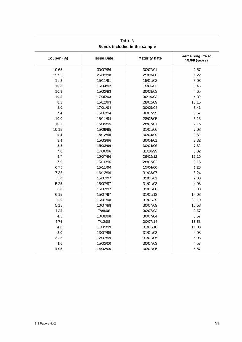
BIS Papers No 2 93
Table 3
Bonds included in the sample
Coupon (%) Issue Date Maturity Date Remaining life at4/1/99 (years)
10.65 30/07/86 30/07/01 2.57
12.25 25/03/90 25/03/00 1.22
11.3 15/11/91 15/01/02 3.03
10.3 15/04/92 15/06/02 3.45
10.9 15/02/93 30/08/03 4.65
10.5 17/05/93 30/10/03 4.82
8.2 15/12/93 28/02/09 10.16
8.0 17/01/94 30/05/04 5.41
7.4 15/02/94 30/07/99 0.57
10.0 15/11/94 28/02/05 6.16
10.1 15/09/95 28/02/01 2.15
10.15 15/09/95 31/01/06 7.08
9.4 15/12/95 30/04/99 0.32
8.4 15/03/96 30/04/01 2.32
8.8 15/03/96 30/04/06 7.32
7.8 17/06/96 31/10/99 0.82
8.7 15/07/96 28/02/12 13.16
7.9 15/10/96 28/02/02 3.15
6.75 15/11/96 15/04/00 1.28
7.35 16/12/96 31/03/07 8.24
5.0 15/07/97 31/01/01 2.08
5.25 15/07/97 31/01/03 4.08
6.0 15/07/97 31/01/08 9.08
6.15 15/07/97 31/01/13 14.08
6.0 15/01/98 31/01/29 30.10
5.15 10/07/98 30/07/09 10.58
4.25 7/08/98 30/07/02 3.57
4.5 10/08/98 30/07/04 5.57
4.75 7/12/98 30/07/14 15.58
4.0 11/05/99 31/01/10 11.08
3.0 13/07/99 31/01/03 4.08
3.25 12/07/99 31/01/05 6.08
4.6 15/02/00 30/07/03 4.57
4.95 14/02/00 30/07/05 6.57

94 BIS Papers No 2
Table 4
Dates of change in benchmark bonds according to different criteria
Benchmark Criteria
Term Coupon(%)
Maturitydate Ours Bloomberg Reuters
5.00 31/1/01
4.25 30/7/02 28/1/99 12/1/99 2/2/993
3.00 31/1/03 2/12/99 4/1/00 19/11/99
5.25 31/1/03
4.50 30/7/04 13/1/99 12/1/99 2/2/995
3.25 31/1/05 2/12/99 4/1/00 19/11/99
6.00 31/1/08
5.15 30/7/09 26/2/99 12/1/99 2/2/9910
4.00 31/1/10 6/10/99 4/1/00 19/11/99
6.15 31/1/13151
4.75 30/7/14 2/12/99
301 6.00 31/1/29
1 Bloomberg and Reuters do not provide benchmark information on these terms.
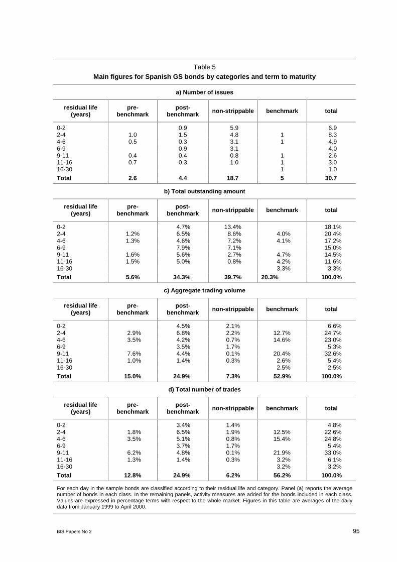
BIS Papers No 2 95
Table 5
Main figures for Spanish GS bonds by categories and term to maturity
a) Number of issues
residual life(years)
pre-benchmark
post-benchmark non-strippable benchmark total
0-2 0.9 5.9 6.92-4 1.0 1.5 4.8 1 8.34-6 0.5 0.3 3.1 1 4.96-9 0.9 3.1 4.09-11 0.4 0.4 0.8 1 2.611-16 0.7 0.3 1.0 1 3.016-30 1 1.0
Total 2.6 4.4 18.7 5 30.7
b) Total outstanding amount
residual life(years)
pre-benchmark
post-benchmark non-strippable benchmark total
0-2 4.7% 13.4% 18.1%2-4 1.2% 6.5% 8.6% 4.0% 20.4%4-6 1.3% 4.6% 7.2% 4.1% 17.2%6-9 7.9% 7.1% 15.0%9-11 1.6% 5.6% 2.7% 4.7% 14.5%11-16 1.5% 5.0% 0.8% 4.2% 11.6%16-30 3.3% 3.3%
Total 5.6% 34.3% 39.7% 20.3% 100.0%
c) Aggregate trading volume
residual life(years)
pre-benchmark
post-benchmark non-strippable benchmark total
0-2 4.5% 2.1% 6.6%2-4 2.9% 6.8% 2.2% 12.7% 24.7%4-6 3.5% 4.2% 0.7% 14.6% 23.0%6-9 3.5% 1.7% 5.3%9-11 7.6% 4.4% 0.1% 20.4% 32.6%11-16 1.0% 1.4% 0.3% 2.6% 5.4%16-30 2.5% 2.5%
Total 15.0% 24.9% 7.3% 52.9% 100.0%
d) Total number of trades
residual life(years)
pre-benchmark
post-benchmark non-strippable benchmark total
0-2 3.4% 1.4% 4.8%2-4 1.8% 6.5% 1.9% 12.5% 22.6%4-6 3.5% 5.1% 0.8% 15.4% 24.8%6-9 3.7% 1.7% 5.4%9-11 6.2% 4.8% 0.1% 21.9% 33.0%11-16 1.3% 1.4% 0.3% 3.2% 6.1%16-30 3.2% 3.2%
Total 12.8% 24.9% 6.2% 56.2% 100.0%
For each day in the sample bonds are classified according to their residual life and category. Panel (a) reports the averagenumber of bonds in each class. In the remaining panels, activity measures are added for the bonds included in each class.Values are expressed in percentage terms with respect to the whole market. Figures in this table are averages of the dailydata from January 1999 to April 2000.

96 BIS Papers No 2
Table 6
Liquidity measures for the Spanish Government Bonds
a) Number of transactions per bond
residual life(years) pre-benchmark post-benchmark non-strippable benchmark
0-2 11.9 0.82-4 4.5 17.4 1.4 43.94-6 6.3 9.5 0.9 54.36-9 13.2 1.99-11 28.0 17.0 0.5 77.211-16 4.6 4.9 0.9 11.316-30 11.3
Total 16.5 16.9 0.3 39.6
b) Trading volume per bond (EUR millions)
residual life(years) pre-benchmark post-benchmark non-strippable benchmark
0-2 90.5 7.02-4 50.0 106.4 9.5 258.24-6 49.5 55.0 5.3 295.96-9 72.0 11.39-11 199.0 89.8 2.5 414.311-16 20.2 28.5 6.8 53.616-30 51.1
Total 45.5 63.2 6.1 153.3
c) Turnover ratio
residual life(years) pre-benchmark post-benchmark non-strippable benchmark
0-2 0.9% 0.1%2-4 2.1% 1.0% 0.2% 2.9%4-6 2.5% 0.8% 0.1% 3.2%6-9 0.4% 0.2%9-11 4.3% 0.7% 0.0% 4.0%11-16 0.6% 0.3% 0.4% 0.6%16-30 0.7%
Total 2.4% 0.7% 0.2% 2.3%
For each day in the sample bonds are classified according to their residual life and category. For each class we compute theaverage of the activity measures for the bonds included. Figures in this table are averages of the daily data from January1999 to April 2000.
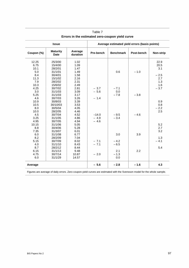
BIS Papers No 2 97
Table 7
Errors in the estimated zero-coupon yield curve
Issue Average estimated yield errors (basis points)
Coupon (%) MaturityDate
Averageduration Pre-bench Benchmark Post-bench Non-strip
12.25 25/3/00 1.02 22.96.75 15/4/00 1.09 20.510.1 28/2/01 1.47 3.1
5.0 31/1/01 1.49 0.6 – 1.08.4 30/4/01 1.58 – 2.5
11.3 15/1/02 2.16 2.77.9 28/2/02 2.31 1.3
10.3 15/6/02 2.49 1.64.25 30/7/02 2.81 – 3.7 – 7.1 – 3.7
3.0 31/1/03 3.09 – 5.6 0.05.25 31/1/03 3.17 – 7.8 – 3.8
4.6 30/7/03 3.26 – 1.410.9 30/8/03 3.39 0.910.5 30/10/03 3.53 0.8
8.0 30/5/04 4.05 – 2.210.0 28/2/05 4.46 2.5
4.5 30/7/04 4.52 –14.0 – 9.5 – 4.63.25 31/1/05 4.86 – 4.9 – 3.44.95 30/7/05 4.94 – 4.6
10.15 31/1/06 5.05 5.28.8 30/4/06 5.28 2.7
7.35 31/3/07 6.01 3.26.0 31/1/08 6.77 3.0 3.98.2 28/2/09 7.04 1.3
5.15 30/7/09 8.02 – 7.1 – 4.2 – 4.14.0 31/1/10 8.43 – 7.1 – 6.58.7 28/2/12 8.44 5.4
6.15 31/1/13 9.48 2.1 2.24.75 30/7/14 10.87 – 2.0 – 1.3
6.0 31/1/29 14.57 0.0
Average – 5.6 – 2.8 – 1.6 4.3
Figures are average of daily errors. Zero coupon-yield curves are estimated with the Svensson model for the whole sample.
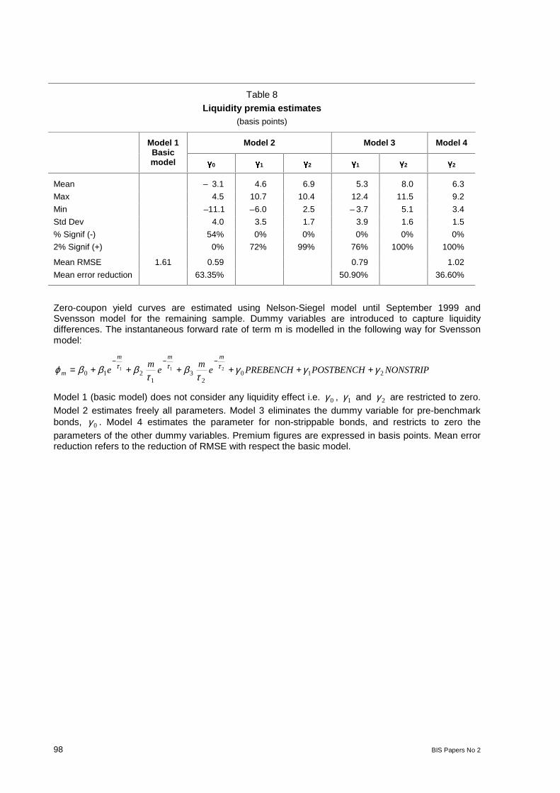
98 BIS Papers No 2
Table 8
Liquidity premia estimates(basis points)
Model 2 Model 3 Model 4Model 1Basicmodel 0 1 2 1 2 2
Mean – 3.1 4.6 6.9 5.3 8.0 6.3
Max 4.5 10.7 10.4 12.4 11.5 9.2
Min –11.1 –6.0 2.5 – 3.7 5.1 3.4
Std Dev 4.0 3.5 1.7 3.9 1.6 1.5
% Signif (-) 54% 0% 0% 0% 0% 0%
2% Signif (+) 0% 72% 99% 76% 100% 100%
Mean RMSE 1.61 0.59 0.79 1.02
Mean error reduction 63.35% 50.90% 36.60%
Zero-coupon yield curves are estimated using Nelson-Siegel model until September 1999 andSvensson model for the remaining sample. Dummy variables are introduced to capture liquiditydifferences. The instantaneous forward rate of term m is modelled in the following way for Svenssonmodel:
NONSTRIPPOSTBENCHPREBENCHem
em
e
mmm
m 2102
31
210211 γγγ
τβ
τβββϕ τττ ++++++=
−−−
Model 1 (basic model) does not consider any liquidity effect i.e. 0γ , 1γ and 2γ are restricted to zero.Model 2 estimates freely all parameters. Model 3 eliminates the dummy variable for pre-benchmarkbonds, 0γ . Model 4 estimates the parameter for non-strippable bonds, and restricts to zero theparameters of the other dummy variables. Premium figures are expressed in basis points. Mean errorreduction refers to the reduction of RMSE with respect the basic model.

BIS Papers No 2 99
Table 9
Impact of withholding tax on liquidity premia estimates(basis points)
Model 5
1 2
Mean 5.4 6.8
Max 12.6 10.5
Min – 3.4 3.8
Std Dev 4.0 1.7
% Signif (-) 0% 0%
% Signif (+) 78% 100%
Mean RMSE 0.82
Mean error reduction 49.06%
Zero-coupon yield curves are estimated using Nelson-Siegel model until September 1999 andSvensson model for the remaining sample. Dummy variables are introduced to capture liquiditydifferences. The instantaneous forward rate of term m is modelled in the following way for Svenssonmodel:
NONSTRIPPOSTBENCHem
em
e
mmm
m 212
31
210211 γγ
τβ
τβββϕ τττ +++++=
−−−
Model 5 is the same as Model 3 but taking into account withholding tax effects for non-strippablebonds. Liquidity premium figures are expressed in basis points. Mean error reduction refers to thereduction of RMSE with respect the basic model (Model 1).

100 BIS Papers No 2
Table 10
Impact of taxes on liquidity premia estimates(basis points)
Model 6
1 2
Mean 3.3 5.0
Max 8.1 7.4
Min – 2.3 3.3
Std Dev 2.6 1.0
% Signif (-) 0% 0%
% Signif (+) 76% 100%
Mean RMSE 0.37
Mean error reduction 77.01%
Zero-coupon yield curves are estimated using Nelson-Siegel model until September 1999 andSvensson model for the remaining sample. Dummy variables are introduced to capture liquiditydifferences. The instantaneous forward rate of term m is modelled in the following way for Svenssonmodel:
NONSTRIPPOSTBENCHem
em
e
mmm
m 212
31
210211 γγ
τβ
τβββϕ τττ +++++=
−−−
Model 6 is the same as Model 3 but using after-tax cash flows. Liquidity premium figures areexpressed in basis points. Mean error reduction refers to the reduction of RMSE with respect the basicmodel (Model 1).
Table 11
Relative liquidity premia with and without taxes(percentage points)
1 0 2 0 1 0+ 1) 2 0+ 1)
Model 3, before-tax yield curve 0.85 1.30 2.07 3.05
Model 6, after-tax yield curve 0.83 1.26 1.98 2.93
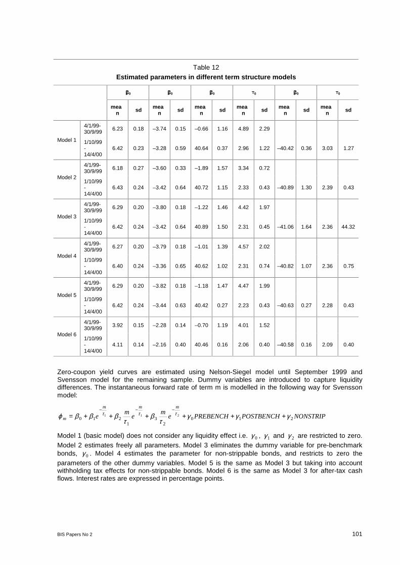
BIS Papers No 2 101
Table 12
Estimated parameters in different term structure models
0 0 0 0 0 0
mean sd mea
n sd mean sd mea
n sd mean sd mea
n sd
4/1/99-30/9/99
6.23 0.18 –3.74 0.15 –0.66 1.16 4.89 2.29
Model 1 1/10/99-14/4/00
6.42 0.23 –3.28 0.59 40.64 0.37 2.96 1.22 –40.42 0.36 3.03 1.27
4/1/99-30/9/99
6.18 0.27 –3.60 0.33 –1.89 1.57 3.34 0.72
Model 21/10/99-14/4/00
6.43 0.24 –3.42 0.64 40.72 1.15 2.33 0.43 –40.89 1.30 2.39 0.43
4/1/99-30/9/99
6.29 0.20 –3.80 0.18 –1.22 1.46 4.42 1.97
Model 31/10/99-14/4/00
6.42 0.24 –3.42 0.64 40.89 1.50 2.31 0.45 –41.06 1.64 2.36 44.32
4/1/99-30/9/99
6.27 0.20 –3.79 0.18 –1.01 1.39 4.57 2.02
Model 41/10/99-14/4/00
6.40 0.24 –3.36 0.65 40.62 1.02 2.31 0.74 –40.82 1.07 2.36 0.75
4/1/99-30/9/99
6.29 0.20 –3.82 0.18 –1.18 1.47 4.47 1.99
Model 51/10/99-14/4/00
6.42 0.24 –3.44 0.63 40.42 0.27 2.23 0.43 –40.63 0.27 2.28 0.43
4/1/99-30/9/99 3.92 0.15 –2.28 0.14 –0.70 1.19 4.01 1.52
Model 61/10/99-14/4/00
4.11 0.14 –2.16 0.40 40.46 0.16 2.06 0.40 –40.58 0.16 2.09 0.40
Zero-coupon yield curves are estimated using Nelson-Siegel model until September 1999 andSvensson model for the remaining sample. Dummy variables are introduced to capture liquiditydifferences. The instantaneous forward rate of term m is modelled in the following way for Svenssonmodel:
NONSTRIPPOSTBENCHPREBENCHem
em
e
mmm
m 2102
31
210211 γγγ
τβ
τβββϕ τττ ++++++=
−−−
Model 1 (basic model) does not consider any liquidity effect i.e. 0γ , 1γ and 2γ are restricted to zero.Model 2 estimates freely all parameters. Model 3 eliminates the dummy variable for pre-benchmarkbonds, 0γ . Model 4 estimates the parameter for non-strippable bonds, and restricts to zero theparameters of the other dummy variables. Model 5 is the same as Model 3 but taking into accountwithholding tax effects for non-strippable bonds. Model 6 is the same as Model 3 for after-tax cashflows. Interest rates are expressed in percentage points.
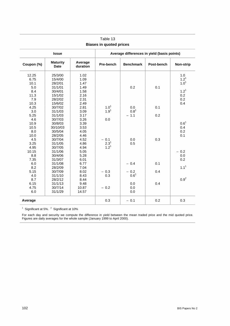
102 BIS Papers No 2
Table 13
Biases in quoted prices
Issue Average differences in yield (basis points)
Coupon (%) MaturityDate
Averageduration Pre-bench Benchmark Post-bench Non-strip
12.25 25/3/00 1.02 1.06.75 15/4/00 1.09 1.21
10.1 28/2/01 1.47 1.01
5.0 31/1/01 1.49 0.2 0.18.4 30/4/01 1.58 1.21
11.3 15/1/02 2.16 0.27.9 28/2/02 2.31 0.2
10.3 15/6/02 2.49 0.44.25 30/7/02 2.81 1.01 0.0 0.1
3.0 31/1/03 3.09 1.91 0.81
5.25 31/1/03 3.17 – 1.1 0.24.6 30/7/03 3.26 0.0
10.9 30/8/03 3.39 0.61
10.5 30/10/03 3.53 0.48.0 30/5/04 4.05 0.2
10.0 28/2/05 4.46 0.14.5 30/7/04 4.52 – 0.1 0.0 0.3
3.25 31/1/05 4.86 2.31 0.54.95 30/7/05 4.94 1.21
10.15 31/1/06 5.05 – 0.28.8 30/4/06 5.28 0.0
7.35 31/3/07 6.01 0.26.0 31/1/08 6.77 – 0.4 0.18.2 28/2/09 7.04 1.11
5.15 30/7/09 8.02 – 0.3 – 0.2 0.44.0 31/1/10 8.43 0.3 0.61
8.7 28/2/12 8.44 0.92
6.15 31/1/13 9.48 0.0 0.44.75 30/7/14 10.87 – 0.2 0.0
6.0 31/1/29 14.57 0.0
Average 0.3 – 0.1 0.2 0.3
1 Significant at 5%. 2 Significant at 10%
For each day and security we compute the difference in yield between the mean traded price and the mid quoted price.Figures are daily averages for the whole sample (January 1999 to April 2000).

BIS Papers No 2 103
Figure 1Life cycle for strippable 10-year bonds included in the sample
0
20
40
60
80
100
120
140ja
n-99
feb-
99
mar
-99
apr-
99
may
-99
jun-
99
jul-9
9
aug-
99
sep-
99
oct-
99
nov-
99
dic-
99
jan-
00
feb-
00
mar
-00
apr-
00
6% 31/1/08 5.15% 30/7/09 4% 31/1/10
0
2000
4000
6000
8000
10000
12000
14000
16000
18000
20000
jan-
99
feb-
99
mar
-99
apr-
99
may
-99
jun-
99
jul-9
9
aug-
99
sep-
99
oct-
99
nov-
99
dic-
99
jan-
00
feb-
00
mar
-00
apr-
00
EUR millions
0.035
0.045
0.055
0.065
0.075
0.085
0.095
0.105
0.115
jan-
99
feb-
99
mar
-99
apr-
99
may
-99
jun-
99
jul-9
9
aug-
99
sep-
99
oct-
99
nov-
99
dic-
99
jan-
00
feb-
00
mar
-00
apr-
00
% Bid-ask spread
Outstanding volume
Number of trades (daily average)

104 BIS Papers No 2
Figure 2Average of daily bid-ask spread
(percentage points)
Source: Reuters-BDE Database
term
0.030
0.050
0.070
0.090
0.110
0.130
0.150
2 4 6 8 10 12 14 16
Duration
spre
ad
pre-bench
post-benchmark
non-strippable
benchmark
%
Figure3
Zero-coupon yield curve(Nelson-Siegel model, 29 March 1999)
2.5
3.0
3.5
4.0
4.5
5.0
0 2 4 6 8 10 12 14 16
Estimated NSTRIPBENCH PRE-BENCHPOST-BENCH
%
Term (years)
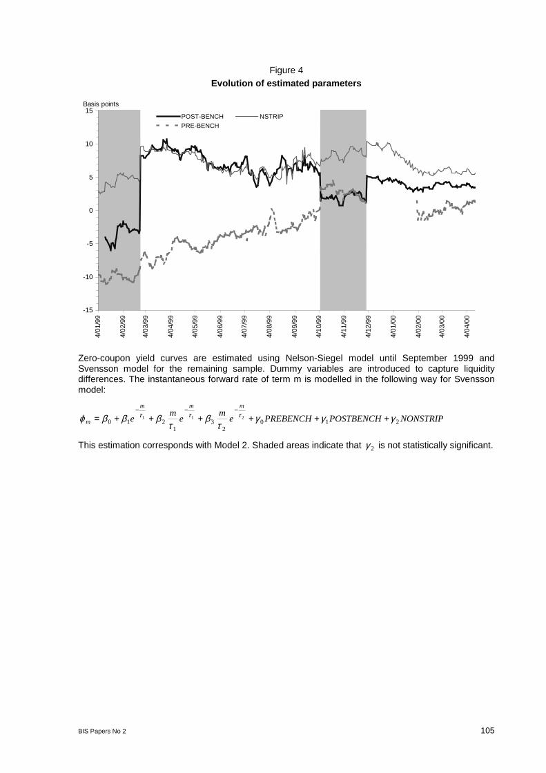
BIS Papers No 2 105
Figure 4Evolution of estimated parameters
-15
-10
-5
0
5
10
15
4/01
/99
4/02
/99
4/03
/99
4/04
/99
4/05
/99
4/06
/99
4/07
/99
4/08
/99
4/09
/99
4/10
/99
4/11
/99
4/12
/99
4/01
/00
4/02
/00
4/03
/00
4/04
/00
Basis points
POST-BENCH NSTRIP
PRE-BENCH
Zero-coupon yield curves are estimated using Nelson-Siegel model until September 1999 andSvensson model for the remaining sample. Dummy variables are introduced to capture liquiditydifferences. The instantaneous forward rate of term m is modelled in the following way for Svenssonmodel:
NONSTRIPPOSTBENCHPREBENCHem
em
e
mmm
m 2102
31
210211 γγγ
τβ
τβββϕ τττ ++++++=
−−−
This estimation corresponds with Model 2. Shaded areas indicate that 2γ is not statistically significant.
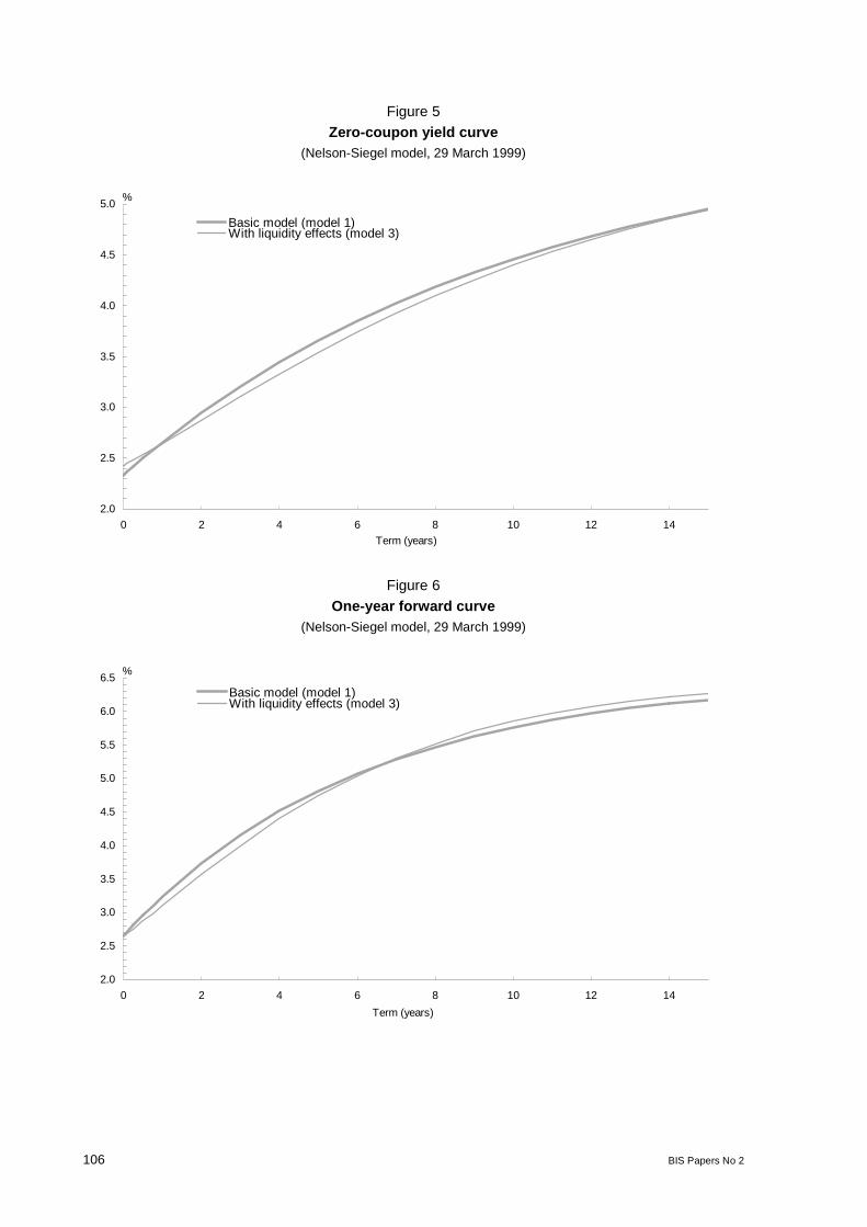
106 BIS Papers No 2
Figure 5Zero-coupon yield curve
(Nelson-Siegel model, 29 March 1999)
2.0
2.5
3.0
3.5
4.0
4.5
5.0
0 2 4 6 8 10 12 14
Basic model (model 1)With liquidity effects (model 3)
%
Term (years)
Figure 6One-year forward curve
(Nelson-Siegel model, 29 March 1999)
2.0
2.5
3.0
3.5
4.0
4.5
5.0
5.5
6.0
6.5
0 2 4 6 8 10 12 14
Basic model (model 1)With liquidity effects (model 3)
%
Term (years)

BIS Papers No 2 107
Figure 7Zero-coupon yield curve
(Svensson model, 31 March 1999)
3.0
3.5
4.0
4.5
5.0
5.5
6.0
0 2 4 6 8 10 12 14
Basic model (model 1)With liquidity effects (model 3)
%
Term (years)
Figure 8One-year forward curve
(Svensson model, 29 March 1999)
3.0
3.5
4.0
4.5
5.0
5.5
6.0
6.5
0 2 4 6 8 10 12 14
Basic model (model 1)With liquidity effects (model 3)
%
Term (years)

108 BIS Papers No 2
Comments on “Estimating liquidity premia in theSpanish Government securities market”
by F Alonso, R Blanco, A del Río and A Sanchís
Christian Upper, Deutsche Bundesbank
Liquidity premia for fixed income securities have commanded increasing attention since their sharpincrease during the summer of 1998. They normally obtained by comparing the yields of two bondswith similar maturity and default risk but different liquidity. Blanco et al follow a more sophisticatedcourse. Instead of pairwise comparisons of two securities, they estimate a zero-coupon yield curve forSpanish government securities and include dummy variables for three categories of bonds which theydeem to be less liquid. The categories are non-strippable post-benchmark bonds, strippable postbenchmark bonds and strippable pre-benchmark securities. The coefficients of the dummies give anestimate for the premium commanded by the corresponding category over a hypothetical benchmarksecurity of the same maturity.
Yield spreads may arise due to a variety of factors, and liquidity differences is only one of them. Theauthors follow a two-step strategy in order to make sure that what they estimate does indeed reflectliquidity premia and not something else. They begin by showing that market liquidity does vary acrossthe four categories of bonds. For my taste, they rely too much on activity indicators such as tradingvolume or turnover ratios. Such variables show that the market was liquid enough in order to handlethe amount of activity observed, but not how easily securities could be traded. However, given thescarcity of readily available measures for market liquidity, the use of activity indicators may beunavoidable. Nonetheless, perhaps the fact that bid-ask spreads increase with maturity does indicatethat shorter term paper is more liquid than longer term paper, although they will not be able to identifythis with their methodology. As a second step, the authors rule out the main alternative factor –differences in taxation - by repeating the estimation with post tax returns. They find that the estimatesfor the coefficients barely change. Hence the interpretation of the yield spread as a liquidity premiumseems acceptable.
The authors find that non-strippable bonds (all bonds issued before July 1997) and post-benchmarkbonds command a yield premium in the range of 5 to 10 basis points over the benchmark, while pre-benchmark issues (on-the-run issues which eventually will become benchmarks) show a negativeyield spread over benchmark paper, although this is significant only about one half of the time.
Let me first make some remarks on the methodology before discussing the results. The procedureused requires considerably more effort than simple pairwise comparisons. So what is the value-addedand is it worth the effort?
Firstly, by using a yield curve as a baseline, the authors reduce the importance of pricing errors forindividual bonds, e.g. due to non-synchronised trading. Such ‚noise‘ should be present mainly in theprices of the less liquid bonds, so that the gain is not so much by using a better benchmark but byaggregating over several bonds in the individual categories. Secondly, using a yield curve reduces thebias that arises because of differing maturities that are sometimes unavoidable in pairwisecomparisons. This should improve the accuracy of the estimates in particular for shorter maturities,where the yield curve tends to be steeper. Thirdly, their approach allows them to test whether theestimates for the yield curve are sensitive to the presence of liquidity premia. Thankfully, they find thatthey are not. This should be of great relieve to all those users of yield curves who do not adjust forliquidity differences.
A final advantage is that their approach allows them to distinguish between the relative importance ofdifferent attributes of a bond in determining the liquidity premium. This would enable us to break downthe liquidity premium into different components. Unfortunately, the authors do not make much out ofthis possibility since the categories into which they group the bonds are mutually exclusive. Forexample, they do not included the non-strippable bonds in the post-benchmark category. As aconsequence, we don’t know whether the liquidity premium of non-strippable bonds over strippablepost-benchmark securities is statistically significant. Using non-exclusive categories would permit themto identify the marginal effects of each attribute.
As in any empirical paper, the question arises whether the variables (in their case the dummies)included are the correct ones. Now I don’t know much about the market for Spanish government

BIS Papers No 2 109
securities beyond what I learned in the paper, so I’m not qualified to make judgements on this issue.However, I wonder why they omitted the volume outstanding of the securities. In Germany, the on-the-run/off-the-run spread is quite sensitive to the size of the issues. Is this not the case in Spain? Anotherpossibility would be to include measures of liquidity in a more direct manner. The authors are right topoint out that the relationship between liquidity premia and liquidity itself is likely to be non-linear, butthis could be dealt with by using dummies e.g. for low/average/high liquidity. Of course, one alwayshas to bear in mind that with only about 30 bonds at any point in time, the number of variables thatone may include is rather limited.
Let me now briefly comment on the results. Figure 4 of the paper shows the evolution of the estimatedliquidity premia over time. Two rather distinct periods can be identified, separated by two months inwhich the coefficient of POST-BENCH turned out to be insignificant. Between March and September1999, the coefficients of NSTRIP and POST-BENCH are virtually identical. As I mentioned before,using non-exclusive categories could have told us whether this was statistically significant. In thesecond period, from December 1999 to April 2000, the two coefficient differ by a much greater extend.That of POST-BENCH declines from 5 to 3 basis points, while that of NSTRIP halves from 10 to 5basis points. Unfortunately, the paper does not discuss the evolution of liquidity premia over time,although this may be due to its more methodological focus. All in all, the movement over time of theestimated premia is rather different from the pattern followed by a (admittedly very simple) measure ofliquidity spreads in the German market, which has seen a sharp rise in liquidity premia during thesummer of 1999. It would be interesting to know why.
Let me conclude by saying that there is a lot of value added in their approach. I found it a veryinspiring paper and I’m looking forward to follow ups. There are two extensions in which I would beparticularly interested. The first would be to go beyond the Spanish market and consider yielddifferences between bonds of different nationalities. At the beginning of August, Spanish 10 yearbenchmark bonds yielded 18 basis points and Portuguese and Italian bonds 26 basis points more thanGerman paper. Why is this the case? Which role does the presence of a liquid futures market for theGerman Bundesanleihe play? These are questions which wait to be answered, although admittedlythe task of putting together a EMU-wide dataset seems aweinspiring. The second extension would beto include credit spreads into the analysis. So far, it has been difficult to disentangle the effect ofcreditworthiness and liquidity. For example, at the Bundesbank, we have argued that the yield spreadof German bank bonds over Bunds mainly reflect liquidity rather than credit premia, but we haven’tbeen able to test this in a rigorous manner. With your methodology, this could be done.

110 BIS Papers No 2
Comments on “Estimating liquidity premia in theSpanish government securities market”
by F Alonso, R Blanco, A del Río and A Sanchís
Oreste Tristani, European Central Bank1
This is an interesting paper that presents quantitative estimates of the premium implicit in the price ofSpanish government securities to compensate investors for liquidity risk and tax factors. The mainresults are obtained fitting a yield curve model through bond prices, measured daily, over the maturityspectrum. The estimation is repeated for the number of available days, from January 1999 to April2000. Liquidity premia are identified through a number of dummy variables attached to less liquidbonds, i.e. issues that are not on-the-run.
The results show that the latter category of bonds appears to command a relatively small premium, ofthe order of a few basis points, broadly comparable to the estimates obtained by Elton and Green(1998) for US government securities. This is reassuring, since it confirms that in developedeconomies, excluding times of market stress, liquidity premia on government securities can beconsidered as negligible in terms of their macroeconomic implications. Nevertheless, their precisemeasurement can be useful in the management of government debt, for example allowing a moreinformed assessment of the relative desirability of alternative issuing practices.
The authors (henceforth ABRS) also mention that knowing the size of liquidity premia on governmentbonds is important for central banks, when they try to extract macroeconomic information (mainly oninflation expectations) from the yield curve. This activity crucially involves filtering out from the curveany kind of risk-premia, amongst which liquidity premia, that are unrelated to macroeconomic factors.The more precise the technique adopted to implement the filtering, the more precise the estimation ofmacroeconomic information reflected in the yield curve.
To filter out liquidity premia, central banks typically concentrate on benchmark issues. However, thismethodology is relatively crude, since liquidity premia (compensation for the lack of immediacy, depth,tightness and resiliency of the market) are likely to characterise all bonds, not just the relatively moreilliquid ones. The assumption that benchmark bonds are not just more liquid, but completely (liquidity)risk-free is not necessarily warranted. To improve the precision of the measurement of inflationaryexpectations implicit in the yield curve, one would really need an estimate of the liquidity premiumimplicit in the return on benchmark issues.
Unfortunately, ABRS’ methodology does not provide indications in this respect, but their exerciseremains interesting for the other reasons emphasised above.
Is the Svensson model precise enough?
As already mentioned, the magnitude of the premia measured by ABRS is “moderately” small, of theorder of a few basis points. In this respect, ABRS’ paper is a commendable effort to look forrefinement and precision in the measurement and estimation of yield curves. A fundamental choice inthe analysis is therefore the selection of the yield curve model. As is often the case in economics, wehave many available models to fit one phenomenon, and no model appears to unequivocally dominatethe others under all circumstances.
ABRS dismiss altogether dynamic models, presumably because, although theoretically moreappealing, their simpler versions do not provide an accurate description of empirical yield curves. Thechoice falls instead on static “estimated” models, such as simple polynomial splines (e.g. the cubic onesuggested by McCulloch, 1971, 1975), which have the advantages of being both manageable and toonly require estimation of a small number of parameters to fit the data. Among the available staticmodels, ABRS favour Svensson’s (1994) modification of the Nelson and Siegel (1987) model. Themain advantage of the Nelson and Siegel model with respect to simple polynomial splines is that thelatter, as noted by Shea (1984), tend to produce unstable forward rates, especially at longer
1The opinions expressed are personal and should not be attributed to the European Central Bank.
BIS Papers No 2 111
maturities. Nelson and Siegel’s formulation, on the contrary, imposes an asymptote on the forwardrates curve, so that the latter always stabilises as the maturity increases. Svensson’s modification ofthis model essentially represents a way to increase the degrees of freedom available in the estimation,so that a larger number of shapes for the yield curve can be accommodated.
Though more stable at long maturities Nelson and Siegel’s methodology is not, however, “perfect”.Like spline models, it essentially amounts to fitting a certain functional form through bond prices. As inany estimation, there will typically be a discrepancy between actual and fitted values. As a result ofSvensson’s modification, the functional form used by ARBS is very flexible and it can accommodate alarge number of shapes for the yield curve. Nevertheless, it will not, excluding exceptionalcircumstances, be able to replicate exactly observed prices. In fact, it is not uncommon for it toproduce fitted yields to maturity that are a few basis points different from observed yields.
Whether this imperfect fit is acceptable will ultimately depend on the scope of the analysis. When zerocoupon rates and long-term forward rates are used to gauge average future inflationary expectations,a discrepancy between actual and fitted values of up to 10 basis points can probably be considerednegligible. Indeed, Svensson takes the view that “for financial analysis, the estimation of forward ratesis done with a number of different methods, some rather complex to achieve sufficient precision. Formonetary policy analysis, the demand for precision is arguably less, which can be traded for increasedrobustness and simplicity of the estimation method”.
Is the extended Nelson and Siegel model sufficiently precise for the estimation of liquidity premia? Ibelieve that the answer is not obvious, since the magnitude of pricing errors generated by theSvensson model is comparable to that of the liquidity premia resulting from ABRS’ estimation. Indeed,liquidity premia are defined as the discrepancy between the observed price of an illiquid bond and theestimated price of a perfectly liquid theoretical bond with the same maturity and coupons. Aninsufficiently precise estimate of the latter would obviously bias the calculation of the premia.
The authors might therefore want to spend some time convincing the reader that it is indeed liquiditypremia that they are measuring, and not (at least in part) a mispricing error due to an insufficientlyprecise model. Since they repeat their yield curve estimation for a large number of days, thus a largevariety of shapes for the yield curve, it should be possible to argue that any potential mispricing error islikely to have zero mean over the days contained in the sample. Hence, even if daily premia couldoccasionally be affected by a pricing error, the average of these premia over the sample period islikely to genuinely represent the compensation for liquidity risk requested by investors.
An alternative model
There are, however, alternative methodologies, such as that presented in Brousseau and Sahel(1999), that allow for a more precise replication of the yield curve.
The fundamental difference between the Nelson and Siegel methodology and that adopted byBrousseau and Sahel is that the latter provides an exact representation of the yield curve, and not astatistical approximation of it. Rather than postulating a certain functional form for the curve, and thenfitting it to the data, Brousseau and Sahel use a non-parametric procedure that allows the shape of thecurve to be (almost) completely data-determined.
This bootstrapped yield curve is defined as one in which the observed prices of all the availablesecurities are replicated without any pricing error. Since only a finite number of bonds is available forthe construction of a continuous curve, the maturities for which no traded bonds are available must,like in the other methodologies, be interpolated. In this case, however, the interpolation is such as toleave the estimates of prices of existing securities equal to their observed values.
A bootstrapped curve obviously bears a more complex mathematical representation than one obtainedthrough, for example, the Svensson methodology. Specifically, it cannot be represented through asmall number of parameters and it can typically only be obtained numerically. Brousseau and Sahelconstruct the curve in an iterative fashion, starting from the available security with the shortest maturityand then moving on by increasing maturity. For illustrative purposes, they concentrate on the US andGerman securities markets and report the results of some bootstrapped curves obtained assumingdifferent sorts of interpolation methods (see Brousseau and Sahel, for details). They then comparethese results with those estimated through a simple spline model.
Interestingly, the difference between the yield curves obtained through the two methodologies turnsout to be, on average, of the order of a few decimals of a percentage point, i.e. potentially large

112 BIS Papers No 2
enough to produce significant differences in the estimation of liquidity premia. This seems to confirmthat some caution is necessary in the interpretation of ABRS’s results. It must be taken into account,however, that the comparison presented in Brousseau and Sahel (1999) is with respect to a simplespline model. Compared to the latter, Svensson’s model is likely to improve significantly the fit of theobserved price data, so that it remains unclear whether its pricing errors can be considered negligiblefor the purpose of estimating liquidity premia.
References
Brousseau, V and B Sahel (1999), “The advantages of using bootstrapped yield curvesfor monetary policy analyses”, paper presented at the ECB Workshop on yield curve modelling,Frankfurt, 29-30 March.
Elton, E J and T C Green (1998), “Tax and liquidity effects in pricing government bonds”, Journal ofFinance 53, 1533-62.
McCulloch, J H (1971), “Measuring the term structure of interest rates”, Journal of Business 44, 19-31.
McCulloch, J H (1975), “An estimate of the liquidity premium”, Journal of Political Economy 83, 62-63.
Nelson, C R and A F Siegel, (1987), “Parsimonious Modelling of Yield Curves”, Journal of Business60, 473-89.
Shea, G S (1984), “Pitfalls in smoothing interest rate term structure data: Equilibrium models andspline approximations”, Journal of Financial and Quantitative Analysis 19, 253-69.
Svensson, L E O (1994), “Estimating and interpreting forward interest rates: Sweden 1992-1994”,NBER Working Paper No. 4871, September.

BIS Papers No 2 113
Does market transparency matter?A case study
Antonio Scalia and Valerio Vacca1
Abstract
We analyse a change in the degree of transparency of MTS, the electronic inter-dealer market forItalian Government bonds, namely the July 1997 move to the anonymity of quotes. Our evidencesupports the hypothesis that a decrease in transparency makes liquidity traders worse-off, whereaslarge/informed traders find it less costly to execute block trades. The evidence is also consistent withthe “waiting game” hypothesis of Foster and Viswanathan (1996): under anonymity, traders tend todelay their trades in an attempt to acquire information through the order flow.
From a public welfare perspective, our results indicate that the move to anonymity has beenaccompanied by an increase in market liquidity and by a reduction in volatility, a phenomenon that isalso partly explained by the growth in Italy’s prospects for early participation in the EMU. The speed ofinformation aggregation on MTS increases, as shown by an improvement of the MTS lead over thefutures market. In a European perspective, the current organisation and performance of MTS place themarket in a competitive position with respect to other sovereign bond markets and may contribute totheir integration under the single currency.
1. Introduction2
The electronic inter-dealer market for Italian Government bonds, known as MTS (from MercatoTelematico dei Titoli di Stato), is characterised in international comparison by a high degree oftransparency (Inoue 1999). In July 1997, 10 years after its inception, MTS switched to a new operationregime in which the names of market-makers who post bid and ask quotes for each security are notrevealed.
The switch seems worth investigating because it prompts a number of interesting questions forfinancial economists and regulatory authorities. What was the reason for the switch? Who benefitedfrom it? How did it affect market performance, in terms of liquidity, efficiency and price volatility? Ismarket microstructure theory consistent with the evidence? Has the switch altered the way ItalianT-bonds are traded on MTS as compared to the over-the-counter market? Can we derive anyregulatory policy lessons from the experience of MTS? What are the implications for the developmentof an integrated sovereign bond market in the European single-currency area?
Market microstructure theory shows that the existence of information asymmetries among participantsis a key element in understanding how a financial market is organised and works. If the market ispopulated by two types of agents with different information endowments and objective functions, thebetter-informed and the liquidity-motivated, then a given market set-up may be optional for one groupbut, generally, not for the other. Similarly, a change in the set-up may benefit one group at theexpense of the other. The dynamic relationship between the two groups has implications for theconsolidation or fragmentation of trading in different markets and for asset price volatility. It can beargued that in a bond market, like ours, the absence of “inside” information on an asset’s fundamentalvalue reduces the scope for heterogeneity of beliefs with respect to a stock market. However, weobserve that the concept of private information must also include knowledge that dealers may acquire
1Banca d’Italia, Monetary and Exchange Rate Policy Department.
2This paper was written as a contribution to the Study Group on Market Liquidity set up by the Committee on the GlobalFinancial System of the G10 central banks. We are grateful for many helpful comments from Masaaki Shirakawa, thecoordinator of the Study Group, Carlo Santini, Michele Bagella, Marco Mazzucchelli, Paolo Angelini, Roberto Violi, ananonymous referee and seminar participants at the Bank of Canada in Vancouver, the Banca d’Italia and the VII FinancialConference at the University of Rome - Tor Vergata. The usual disclaimer applies. The views expressed herein are those ofthe authors and do not involve the responsibility of the Banca d’Italia. Correspondence address:e-mail: [email protected].

114 BIS Papers No 2
on the order flow and on the trading intentions of large customers, an argument which applies to thebond and foreign exchange markets as well as to the stock market. This knowledge causes an updateof beliefs and may be profitably exploited at the expense of other market participants, according to anotion that is also at the basis of the literature on block trading and dual-trading. From an empiricalviewpoint, some studies support this hypothesis in the forex market and in the bond market (see Lyons1995 and Scalia 1998a), although there is also evidence to the contrary (Proudman 1995).
The models of information asymmetry point to one conclusion: liquidity traders in general prefer moretransparency, informed traders prefer less transparency. This notion was pioneered by the Grossman(1998) model of sunshine trading. Sunshine trading, ie disclosing pre-trade information on the directionof price-contingent orders, removes the possibility that those orders are information-based and thuseases the inference problem of market-makers. This should lower execution costs for sunshine tradersand possibly increase overall trading volume. Forster and George (1992) explore the effects of variousdegrees of traders’ anonymity on the distribution of wealth within the two groups of marketparticipants. They conclude that if monitoring who is trading in a centralised system gives informationon liquidity trades, then disclosing the identity of current participants lowers execution costs for liquiditytraders, provided that there is sufficient competition among privately informed agents. This clearlyreduces the expected profit of informed traders. The analysis of Pagano and Röell (1996) providessimilar results: in a comparison of alternative trading systems, it is shown that greater transparency,such as that provided by a centralised order execution system with full disclosure, reduces theaverage trading cost for liquidity traders. Madhavan (1995) examines the issue of post-tradeinformation disclosure and market fragmentation vs consolidation in a two-period dynamic model. Themodel provides an unambiguous prediction on the implication of different disclosure rules for informedtraders and “large” (or strategic) liquidity traders: they should prefer non-transparency because itfacilitates dynamic trading strategies, like “working” a large order over time. Without mandatorydisclosure, dealers also prefer not to disclose trades voluntarily because they profit from the reductionin price competition. Naik, Neuberger and Viswanathan (1994) investigate the relationship betweendelayed trade disclosure rules and execution costs in a dynamic market setting with risk aversedealers. If there are two stages of trading, first a public investor who trades with market-maker A, andthen A who trades with other competing market-makers, a delayed disclosure rule of the first-roundtrade by A grants him the possibility in the second round to exploit the information conveyed by thetrade itself. In turn, A passes on part of the associated profit to the public investor. The authors stressthe fact that their conclusion has a more general bearing: any time less-than-full disclosure of largeand informative orders occurs, the dealers who intermediate the order and their customers should bebetter-off.
Our summary of models that explore the effects of information asymmetry and market transparency isfar from exhaustive. However, theory provides an unambiguous prediction in our context: underassumption that significant informational asymmetries exist, the switch that took place on MTS in July1997 should have shifted the balance between liquidity traders’ and informed/large traders’ profits infavour of the latter. For the purpose of the tests to be conducted in the following sections, we set forthtwo hypotheses:
• Hypothesis I: liquidity traders have been made worse-off by the move to anonymity (we shallcall this hypothesis the “liquidity trader’s curse”).
• Hypothesis II: (the “large trader’s blessing”): large/informed traders have been madebetter off.
Our brief survey also suggests a third implication, related to the previous ones. By not disclosing thenames of market-makers, the 1997 switch has made the structure of MTS more similar to that of theover-the-counter inter-dealer broker market, where dealers negotiate trades without revealing theiridentity. We should consider the possibility that dealers in the opaque over-the-counter market (tradingeither through a broker or vis-à-vis) benefit from the price discovery function of the highly transparentMTS, thus free-riding on the information disseminated by the latter (see also Madriagal 1996). Hence,before the 1997 shift there would have been two types of free-riding. The first would have been amongMTS members, and it is captured by Hypothesis I. The second would have been by the OTC market atthe expense of MTS. If the switch to anonymity has reduced the second type of free-riding, makingMTS more similar to the OTC market, then the incentives for the informed/large dealers to trade over-the-counter rather than on the regulated market have declined. We have the following hypothesis:
• Hypothesis III (“decline of OTC free-riding”): trading volume on the OTC market has fallensince the MTS shift.
BIS Papers No 2 115
The events that preceded the market move seem broadly consistent with Hypothesis I-III. At the end of1996 the proposal of anonymity was put forward by a group of MTS specialists (which we mayassimilate to the informed/large traders of theory), led by one with foreign affiliation. The mainargument advanced by the proponents was that the shift would increase the welfare of the most skilledmarket players, thus enhancing competition and market efficiency. In fact, the proponents’ complaintabout the regime of full transparency was that it allowed small dealers to mirror the moves of the bigplayers. Understandably, some small traders had reservations. The treasury and the Banca d’Italiaraised no objections. In the end the management board (in which small dealers are lowly represented)approved the proposal, which became effective on 14 July 1997.
The MTS switch of 1997 is also interesting for another reason. Foster and Viswanathan (1996) haveexplored the possibility that informed traders’ signals are different, giving an incentive to informedtraders to forecast the price forecasts of others. This may induce each informed trader to delay histransactions and wait for the other traders’ moves to reveal more information. The Foster-Viswanathanmodel has the following prediction for intraday trading activity on MTS.
• Hypothesis IV (the “waiting game”): after the switch to anonymity, the increasing dispersionin traders’ opinions reduced market turnover in the early stages of trading and increased it inthe later stages.
The previous discussion explains the first objective of this paper. By analysing various marketindicators before and after the MTS switch to anonymity, we wish to conduct a test of the four abovementioned hypotheses: the liquidity trader’s curse, the larger trader’s blessing, the decline of free-riding and the waiting game hypothesis. Another contribution of our test is that we use an original andextensive data set as compared to that of the existing literature.
Should the hypothesised worsening of terms for liquidity traders be the unique, or even the mainconcern for market regulators? This question raises the more general problem of which market designmaximises public welfare, which brings us to the subject of normative economics and regulatorypolicy. O’Hara (1995) tries to qualify the three goals of a market set forth by Domowitz (1990). Theyare (i) reliable price discovery, (ii) broad-based price dissemination, and (iii) effective hedging againstprice risk.
Concerning the first goal, O’Hara argues that the ability to find a market-clearing price is enhanced byscale and possibly by the existence of multiple settings which suit the needs of different types oftraders.
The achievement of broad-based price dissemination is a more contentious issue because the free-riding problem discussed earlier sets up a trade-off between market transparency and the pricediscovery process in the same market. Broadly speaking, market transparency certainly improvespublic welfare. However, in a dynamic setting, if the same asset is traded in market A and market B,and market A becomes more transparent, then it is possible that large/informed traders will move fromA to B. In this case, it is conceivable that the price discovery process in market A will diminish, to theadvantage of market B.3 Therefore, it is not clear where on the ideal market transparency scale thecosts from a reduction in informed trading will outweigh the benefits from greater informationdissemination (see eg Franks and Schaefer 1995). This issue is at the heart of our investigation.
The third goal, namely hedging of price risk, reflects the concern for the market’s ability to provideinsurance to liquidity traders. The empirical counterpart of this goal is the minimisation of executioncosts for liquidity trades and the improvement in general of market liquidity, defined as the propertywhereby the price impact of an order is small. O’Hara introduces a fourth goal of optimal marketdesign:
“(…) another, perhaps greater, function of the market that is not recognised in theworking definitions given above (…) is the role of market efficiency. How well andhow quickly a market aggregates and impounds information into the price mustsurely be a fundamental goal of market design.”
3The above statement has no precise implications on the change in the degree of price discovery that derives from a changein the transparency of A for the whole market, given by the sum of A and B.
116 BIS Papers No 2
However, she also notes that the search for market efficiency presents two main problems. First,raising the speed of information aggregation may in principle increase price volatility, which is notdesirable. Second, since market efficiency is positively related to the extent of information-basedtrading, which in turn generates losses for liquidity traders, the goal of efficiency may conflict with thatof minimising execution costs for the uniformed. To summarise, although the issue of the optimaldesign of a financial market remains in O’Hara’s words an open question, it seems safe to claim that,provided “sufficient” scale and transparency, the contribution of a market to public welfare should bemeasured along three dimensions: liquidity, volatility, efficiency (where the second variable clearlyexerts a negative effect).
We observe that in the case of the government bond market the pursuit of public welfare along theselines is consistent with the objective of minimising the cost of public debt servicing and with theoperating objectives of the monetary and regulatory authorities (Santini 1997): to carry out liquiditymanagement operations that do not affect the smooth functioning of the market, to obtain informationabout market expectations, to improve monetary policy implementation in general, to conductmicro-prudential policy.4
The second objective of our empirical investigation is therefore of a regulatory nature. Becausenormative economics in this area does not show unambiguously what is the welfare-maximisingdegree of market transparency, we wish to develop a case study based on the previously noted event.We observe a change of regime in the arrangement of our market. By estimating the threeperformance variables defined earlier, both before and after the shift, we try to empirically assesswhether it afforded a higher or lower level of welfare. We shall also try to keep into account animportant macroeconomic factor that may have influenced the performance of MTS during our sampleperiod, namely the fiscal consolidation process which brought about a sharp improvement in Italy’sprospects for early participation in the European Monetary Union. To this extent, we shall provideestimates of the relative weight of the microeconomic effect on our market performance measures, asdistinct from the microeconomic effect related to the shift to anonymity.
The paper proceeds as follows. Section 2 describes the main features of the market. Section 3presents evidence and tests on Hypotheses I-IV. Sections 4-6 provide estimates and tests on marketliquidity, volatility and efficiency, respectively. Section 7 discusses the empirical evidence against thebackground of theory, the regulatory implications and the prospects for the development of anintegrated securities market in the single currency area. Section 8 summarises and concludes. AnAppendix table provides a brief history of the Italian government bond market during the last decade.
2. The market
The securities listed on MTS include all recent Italian Treasury issues: the three-, six- and 12-monthbills known as BOTs, the 18- and 24-month bills known as CTZs, the floating-rate notes with initial lifeof seven years known as CCTs, and the fixed-coupon BTPs with initial life of three, five, 10 and 30years. The minimum order size is five billion lire, which is by far the modal trade size. Market membersare of three types: specialists, primary dealers and ordinary members.5 Specialists and primarydealers are committed to quoting firm two-way quotes on a wide range of securities, to beingcompetitive in terms of tightness of spreads, and to maintaining a share on the primary and secondarymarket above a certain threshold, with stricter requirements applying to specialists.6 Both categoriesmay apply for bond and cash lending with the Banca d’Italia. Ordinary members can trade at thequoted prices. Specialists and primary dealers can also trade at somebody else’s quotes.7 In practiceover 60% of transactions take place between two market-makers (specialists and primary dealers). In
4A detailed survey of market structure and regulation in government securities markets is provided by Dattels (1995).
5Strictly speaking, specialists are included in the class of primary dealers. Upon demand and subject to the selection criteriaset by the Treasury and the Banca d’Italia, a primary dealer may be upgraded to the status of specialist. Downgradedspecialists maintain the status of primary dealers.
6The requisites for specialists are market share above 3% on the primary market and above 1.5% on MTS. Primary dealersmust maintain a minimum share of 0.5% on MTS.
7The July 1997 shift to anonymity was accompanied by a further innovation: all quotes at the same price made by differentmarket-makers are aggregated, leading to an aggregate volume figure associated with each outstanding quote.
BIS Papers No 2 117
what follows we shall refer to the players who initiate a trade as “traders”, without distinguishingwhether they are market-makers or ordinary members.
Trading hours are from 09:00 to 17:10. The market trading mechanism is fully integrated. Eachmember’s video-terminal serves three functions: (1) publication of pre- and post-trade information,including the five best bid and ask quotes for each security,8 (2) trade execution at a key-press, and(3) automatic clearing and settlement onto the centralised systems for bank reserves and governmentbonds managed by the central bank.9
In the spring of 1997 the run-up to the annual review of the specialists’ requisites, including a check oftheir market share, contributed to the growth in overall trading volume observed on MTS. Somespecialists may have inflated their transactions on an intraday basis, without affecting their openpositions at the end of the day, in an attempt to improve their turnover score. After the June 1997review, the Treasury and the Banca d’Italia decided to lengthen the observation period to two yearsand to hold the next review in January 2000.10 Partly as a consequence of this process, daily tradingvolume changed from an average 36 trillion lire in the second half of 1996 to 45 trillion in the first halfof 1997; since then, it has stabilised at around 33 trillion lire.
The data-set employed in the empirical analysis of the following sections includes all MTStransactions, and the identity of the traders, in the period from 1 September 1996 to 31 May 1998. Theold regime data sample runs from 1 September 1996 to 13 July 1997 (period 1). The new regimesample goes from 14 July 1997 to 31 May 1998 (period 2). The two samples are approximately equalin length, about 10½ months each. To be precise, there are 213 working days in period 1 and221 working days in period 2.
3. Evidence on theoretical predictions
3.1 Hypothesis I - The liquidity trader’s curse
The first type of evidence we should like to gather is that concerning the change, if any, in the degreeof market participation by the informed/large dealers and the liquidity/small traders. To this extent,Table 1 provides summary statistics on the average number of active traders on a daily basis, rankedaccording to their market share, before and after the switch to anonymity. If we consider the smallesttraders (below 0.1% of trading volume) we note that they decrease in number from 15 in period 1 tothree in period 2. The second smallest class of traders (between 0.1% and 0.25%) decreases from110 to 84. The third class (between 0.25% and 0.5%) increases slightly from 59 to 65 traders. Thefourth class (0.5 to 1%) increases from 34 to 41 traders. Overall, if we set a threshold for “small”traders at 1%, we note that their average number decreases from 218 to 193. The two classes of thelargest traders, from 1 to 2.5% and above 2.5%, both increase, with their sum going from 42 to48 traders. The reduction in the number of small traders is also evidenced by the data on marketconcentration, provided in the lower part of the table. The Herfindahl concentration index of tradersincreases from 3.2 to 3.8%. The degree of concentration measured on the market-makers’ sideincreases from 5.0 to 5.8% on average. The null hypothesis of equal means before and afteranonymity is rejected. These results are consistent with Hypothesis I.11
3.2 Hypothesis II - The large trader’s blessing
The greater concentration among market-makers seems consistent with the hypothesis that largetraders have been made better-off. The category of informed and/or large traders can also be detectedex post based on the occurrence of large trades. On MTS a “block trade” as such hardly ever occurs.Due to the prudence of market-makers who post firm quotes, also in terms of size, 99% of transactions
8Prices are quoted clean, as a percentage of par value.
9Further details on the functioning of MTS can be found in Banca d’Italia (1994).
10The switch to anonymity was also viewed as a measure to avoid the inflation of trading volume.
11The daily behaviour of the concentration indices has a mixed pattern. It is relatively stable in the first half of each year, but ittends to increase slightly towards year-end.

118 BIS Papers No 2
occur at or below five times the minimum size of five billion lire. Traders wishing to exchange a largeamount of bonds respond to this behaviour by working the order over time. This would suggest toproxy large trades by tracking down the continuations of trades made by the same trader on the samebond on each working day. Things are complicated, however, by the fact that during our sample perioda “race for volume” took place (see previous section), and many trades were inflated, ie offset bytrades of opposite sign within the same day. To control for this phenomenon, we proxy large trades asfollows. Within each working day, we compute the net daily change in each trader’s holdings of eachlisted bond. When the net change in absolute terms is larger than a given threshold, we count one“large trade” for each continuation of trades above the same threshold. Our working variable is thendefined as the ratio of large trades so defined to total daily volume.
The evidence is presented in Figure 1, Panel A, for a threshold of 50 billion lire, and Panel B, for athreshold of 100 billion lire. Each panel reports the daily series of the large trade ratio and aninterpolating function. In the case of a threshold of 50 billion lire, the ratio generally lies between10% and 20%. Panel A shows that the series increases from period 1 to 2, and the tests of equalmean and of equal distribution across periods are rejected. The series obtained with a threshold of100 billion lire generally lies between 0% and 10%. The evidence across periods in analogous: theratio increases from period 1 to period 2, indicating that, under anonymity, it has become easier tobuild/unwind large positions on MTS, and the tests of equal mean and distribution are rejected. Thesefindings support Hypothesis II.
3.3 Hypothesis III - The decline of OTC free-riding
In order to gather evidence on the hypothesised shift from OTC to MTS transactions, we used theinformation contained in the monthly statistical reports of MTS market-makers to the Banca d’Italia.These reports include the OTC trading volume in government bonds of each dealer, with a breakdownfor trades carried out with residents and non-residents. We corrected the residents’ figures for theeffect of double counting by scaling them down by the share of MTS turnover involving trades betweentwo market-makers. We thus obtained an estimate of the OTC volume that is comparable with theMTS exact figures that we possess. We then calculated the ratio of OTC volume over total inter-dealervolume (OTC plus MTS). The resulting figures are given in Table 2. It shows that the OTC share tendsto increase from the end of 1996 onward. The highest OTC share figures are observed in July 1997(37.3%) and in May 1998 (39.6%). The subdued OTC share in the spring of 1997 may partly beexplained by the race for volume that took place on MTS and that no longer occurred underanonymity. The evidence of Table 2 is at odds with Hypothesis III.
3.4 Hypothesis IV - The waiting game
If the waiting game hypothesis holds, dealers should try to delay their trades on an intraday basis inthe attempt to acquire more information through trade flow, and we would expect a shift of tradingvolume for the early stages of trading to the later stages. In order to analyse intraday turnover on MTS,we chose the benchmark 10-year BTP issue, which is generally the most heavily traded security. Theevidence is given in Figure 2, which shows the intraday relative volume on the benchmark BTP, ie theshare of trading volume observed in each half-hour interval of the day over the total daily volume ofthe bond. The key findings that emerge from Figure 2 are as follows. First, trading volume increasesfrom the first half-hour of trading (09:00-09:30) to the second half-hour. Second, like in most financialmarkets, there is a decline in trading activity after 12:30 for about 1½ hours. Third, trading activityremains steady after 14:30 (we recall that the closing interval after 17:00 lasts only 10 minutes, ie onethird duration of the other intervals). Finally, we note that from period 1 to period 2 volumes declineslightly in the morning intervals and increase correspondingly in the intervals after 14:30. In fact, 3.2%of total daily volume shifts from trading before 14:30 in period 1 to after 14:30 in period 2. Thehypothesis of identical distribution of volumes is rejected in nine out of 17 intraday intervals by theKolmogorov-Smirnov test. The hypothesis of identical means is rejected in six out of 17 intervals bythe t-test. The last finding seems consistent with Hypothesis IV.
4. Liquidity
Various definitions have been provided in the literature for the concept of market liquidity. Perhaps themost popular one is “a market is liquid if the impact of a trade on price is small”. However, the liquidityconcept has several other dimensions (see eg O’Hara 1995; Muranga and Shimizu 1997). The

BIS Papers No 2 119
richness of our data-set allows us to conduct an empirical study of market liquidity along differentdefinitions. The first and simplest indicator of market liquidity is turnover. For the reason explained inSection two, namely that trading volume should have been biased by the dealers’ effort to maintaintheir status before the June 1997 review, we do not think that it is useful to compare total MTS tradingvolume before and after the market move to anonymity. Instead, we prefer to focus our attention onthe number of bonds that were actively traded on each day. The second indicator of liquidity is the bid-ask spread. The (half-) spread is the reward paid by traders to market-makers for their services, whichprovides immediacy to those wishing to buy or sell a security. The third indicator of liquidity is themarket impact of a trade, which is related to the adverse selection problem faced by market-makersand which varies directly with the perceived arrival of orders from informed traders. We present theevidence on each of the above mentioned indicators respectively in the three following subsections.
4.1 Active bonds
We choose two statistics to describe turnover on the active bonds. We first rank the bonds traded oneach day by their volume of transactions. We then consider those bonds below the median and take(1) their number (ie one half of the total number of traded bonds) and (2) their share over total dailytrading volume. These statistics are plotted on a daily basis in Figure 3. It shows that the number ofthe 50% least-traded bonds tends to increase in period 1, and thereafter it declines slightly. Onaverage, this number changes from 63.6 in period 1 to 65.1 in period 2. On the other hand, the volumeshare of the least traded bond shows an increasing trend, and it doubles on average from 6.9% beforeanonymity to 14.3% after anonymity. The tests of the hypotheses that the mean and distribution ofmarket share by class do not change are rejected.
We note that in addition to the review of the specialists’ status (see Section 2), there were also reviewsof the primary dealers’ status at the end of 1996 and 1997. One of the requisites was related to eachdealer’s ability to make a market in the illiquid bonds. We attribute the observed increase in the shareof the least traded bonds at year-end to the dealers’ attempt to qualify in the annual review. Thisphenomenon seems to have been particularly significant at the end of 1997.
4.2 Bid-ask spread
Our intraday data-set does not include data on the bid-ask spread. In order to obtain estimates of thefixed-cost of trading associated with the existence of the spread, we use our intraday transactions datato fit the two-equation empirical model of trade and quote revision proposed by Foster andViswanathan (1993) (see Hasbrouck 1991 for a thorough discussion). This model is as follows:
(1)
(2)
Where qt is the signed trade size (eg –5 indicates a public scale of five billion lire at the current bidprice) and dpt is the price change that occurred between the previous trade and the current trade. 1dt=i
is an indicator variable equal to one if trade t occurs in the i-th half-hour interval of the day and 0otherwise. 1qt=0 is an indicator variable equal to 1 if trade t is a public buy and 0 otherwise. Equation
(1) tries to model the expected value of the incoming order conditional on the past record of ordersand prices; the residual t is the unexpected component, or the innovation brought about by the orderand potentially related to informed trading.12 The residual in turn becomes one of the explanatoryvariables of the price change caused by the order, given by the equation (2). In it, the coefficient c isan estimate of the “fixed” component of transaction costs. Assuming that the “true” (and unobservable)value of the bond does not change, c measures the difference between the transaction price and thetrue price, corresponding to one half of the spread, ie to the compensation for the market marking
12Equation (1) is run using the logit method.
tk
ktkjtj
jid
N
iit qdpq
tτιβδα ++++= ∑∑∑
=−−
==
=
3
1
3
12
1
[ ] [ ] ∑∑=
==>>=
>> +++−+−=−−
N
jttjdjtidqq
N
iiqqt vccdp
tttttt2
002
00 1111211211
τλλτ
120 BIS Papers No 2
services provided by the dealer who posted the quote. In practice, since the true bond price doeschange over time, if we take 2c we do not obtain the actual spread but an unbiased (and noisy)estimate of it.13 In equation (2) we allow for the possibility that 2c changes during the day, byintroducing dummy variables for the half hour intervals i = 2,…,N, where N is the last interval of the adverse selection component of trading cost, or market impact of a trade, which enters the total cost oftrading when the trade itself is not expected by the market-makers on the basis of the past order flow. ! ! N-1) intervaldummies. This estimation approach, which recognises the dynamic nature of trading costs, is similarto those employed in a number of previous studies.14
The evidence on the intraday spread estimates for the benchmark 10-year BTP is plotted in Figure 4.The first fact that we note is that 2c is roughly W-shaped during the day. The spread has three peaks:at the open, before 14:30 and at the close. The peak between 14:00 and 14:30 (08:00-08:30 USEastern Standard Time) is related to the market’s uncertainty concerning the opening prices of theUnited States financial markets. The peak may also be related on some days to the upcoming releaseof United States’ macroeconomic indicators. This finding is analogous to previous evidence for MTS(Scalia 1998a) and to the behaviour of the United States’ T-bond market (Fleming and Remolona1997). The second fact that we note is that the spread in period 2 is uniformly lower than in period 1.In particular, the spread in the initial and final intervals of the day declines from 2 to 1.4 basis points ofprice.
It may be argued that the estimated reduction of the spread, which is positively related to the asset’sexpected volatility may have been caused by the general improvement in the Italian Treasury bondmarket, brought about by the increase in Italy’s prospects for early participation in the EMU. Thisposes the problem of distinguishing the effects that MTS anonymity and the macroeconomic changehave had on our market performance variables. As a control variable for macroeconomicimprovement, we chose the 10-year BTP-Bund-yield differential.15 Figure 5, Panel A shows the seriesof the estimated bid-ask spread and the BTP-Bund yield differential on a daily basis. This yielddifferential fell from around 3% in September 1996 to 1% in July 1997 and fell again to 0.25% in May1998. The bid-ask spread series shows a declining trend in period 2. In that period the differential andthe spread are clearly associated.16
What are the relative weights of the micro- and macroeconomic effects on the spread? In order toprovide an answer, we run a regression of the spread estimate over a constant, the differential adummy equal to one in the second period, and the product of the previous two variables. The weightsare obtained as the product of the estimated coefficients by the average value of each variable, as apercentage of total. These weights are reported in Figure 5, Panel B. The weight of the microeconomiceffect, related to the dummy variable, is equal to 56%. The macroeconomic variable, ie the differential,accounts for 10%, and the third variable (the differential times the dummy) accounts for 34%. Adoptinga cautious stance, and attributing the last estimate entirely to the macroeconomic effect, we observethat the microeconomic effect accounts for over one half of the total improvement in the bid-askspread from period 1 to period 2.
13In order to control for residual heteroskedasticity caused the different length of time between subsequent trades, we weighteach observation in equation (2) by the inverse square root of the time elapsed since the previous trade. We thus runequation (2) with the weighted least squares method.
14Equation (2) is instantaneous, ie there are no lagged effects of prices or quantities. According to Hasbrouck (1991), theinclusion of lagged terms in the price equation would be justified under the following circumstances: (a) inventory effects arein place, such that dealers seek to smooth the holdings of bonds over time; (b) there is “price-discreteness”, due to a largetick-size; (c) prices adjust slowly to new information. In our setting, we think that the case for hypotheses (a)-(c) is weak, andthe inclusion of lagged terms would only affect the efficiency of the estimates. Therefore, we see no compelling reason fordeparting form the Foster-Viswanathan instantaneous-modelling approach. The average adjusted R-square of our dailyequations is equal to 0.36.
15Another plausible proxy might be the market perceived probability of Italy’s early participation in the EMU. This estimatedprobability measure and the BTP-Bund spread are strongly correlated.
16This is confirmed by a simple regression of the spread over a constant and the differential (not reported for simplicity). Wealso perform a Chow stability test that the regression coefficients are identical between period 1 and period 2. The resultsshow that the differential is directly related to the spread; however, this effect is limited to period 2, and the stability test isrejected.

BIS Papers No 2 121
4.3 Market impact
The " #$% " 2 there is a tendency "% lower in period 2 than in period 1.
& !! "'#, Panel Ashows the market impact series and the yield differential series. The evidence, again, is that thedifferential is positively related to the spread in period 2, but unrelated to it in the earlier period.17
The results on the weights of the micro- and macroeconomic effects are given in Panel B, obtainedwith the same methodology of the previous subsection. The microeconomic effect turns out to beextremely large, equal to around 69% of the total price impact. The macroeconomic effect accounts forthe remaining 31%.
5. Volatility
We estimate volatility on an intraday basis as the squared log-difference of the bench mark 10-yearBTP prices, taken at half-hourly intervals. The resulting evidence is presented in Figure 8. Intradayvolatility displays a U-Shape. Although its estimate declines in the last interval of the day, we recallthat the different length of the interval itself does not make the corresponding value comparable toestimates for earlier intervals.18 Volatility is largest in the initial interval of period 1, when it is equal to0.03%. Throughout the rest of the day it is much lower, generally below 0.015%, and it rises after14:30. The second fact that we note is that volatility in period 2 is uniformly lower than in period 1. Inparticular, volatility in the first half hour of trading declines from 0.030 to 0.011. Moreover, after 14:30the increase in volatility is less pronounced.
Figure 9, Panel A provides evidence on the relationship between the BTP-Bund yield differential andvolatility on a daily basis. The picture is slightly different from the case of the spread and marketimpact. A direct relationship between yield differential and volatility is found; this is significant inperiod 2 only; however, the Chow stability test between periods can not be rejected. The evidence ofpanel B is that the microeconomic effect has a weight of 37% on volatility, ie much smaller than in thecase of the cost measures, whereas the macroeconomic effect accounts for the remaining 63%.
6. Efficiency
The notion of financial market efficiency implies that prices fully reflect all available information. As iswell known, Fama (1970) distinguishes three types of efficiency: weak form efficiency, whichrequires that no investor can earn excess returns based on historical price information; semi-strong-form efficiency, which implies that no investor can earn excess returns by applying trading rulesbased on any publicly available information; and strong-form efficiency, which implies that noinvestor can earn excess returns using any type of information, whether public or private. Whilestrong-form efficiency is unachievable if one accepts the view that information asymmetries are arelevant factor in explaining dealers’ behaviour, weak-form and semi-strong-form efficiency are inprinciple attainable by a financial market. In particular, the hypothesis of weak-form efficiency hasbeen tested by empirical studies on leads and lags between cash and futures markets for the samesecurity, in which prices are strictly correlated due to a no-arbitrage argument. The evidence in thecase of bond markets is available for Japan and Italy. In Japan the JGS inter-dealer cash market isdriven by the futures market, with cash prices lagging behind the price of the 10-year JGS contracttraded on the Tokyo Stock Exchange by two minutes on average (Miyanoya, Inoue and Higo 1997). Inthe case of the Italian BTPs there is evidence of reciprocal causality between the futures contracttraded on LIFFE and the benchmark 10-year BTP traded on MTS in the years 1992-1993; furthermore,
17The Chow stability test between period 1 and 2 is rejected.
18Under the hypothesis that bond prices follow a Brownian motion, our (squared) volatility proxy in the last interval should bemultiplied by 30’/10’=3 in order to express it in half-hourly terms.
122 BIS Papers No 2
the futures lead can not be exploited to earn excess returns on MTS, consistent with weak-formefficiency of MTS with respect to LIFFE (Scalia 1998b; see also Angeloni et al 1996).
Has MTS changed its record of efficiency with respect to LIFFE following its switch to anonymity? Thisquestion is relevant because traders in the two marketplaces are not fully integrated, particularlyconcerning their access to information on monetary policy implementation, the Treasury’s issuingdecisions and the order-flow. The empirical analysis that follows seeks to update previous evidence,while improving the type of data and the power of the causality test.
Our data sample includes all MTS transactions on the benchmark 10-year BTP and all BTP futurestransactions at LIFFE in the period from September 1996 to May 1998.19 We also employ an intradaydata-set, obtained from the Reuters service, that contains market prices and quotes at five-minuteintervals on the following financial instruments: the three-month eurolira futures contract at LIFFE (lasttrade price), the Deutsche Mark/US Dollar exchange rate (last bid), and the 10-year Bund futurescontract traded at LIFFE (last trade price). The general motive for the inclusion of these variables in aVAR analysis of causality is to take into account the behaviour of the world financial markets thatpotentially may explain the behaviour of BTP prices, ie we should like to include in a parsimonious wayall the relevant information set. We observe that, compared with previous studies, we take a step fromthe notion of weak-form efficiency to that of semi-strong-form efficiency, which involves thepredictability of prices based on all publicly available information. The specific reasons for this set ofvariables are as follows. The short-term rate futures captures the attitude of domestic monetary policy.The DM/USD exchange rate is the reference exchange rate for Europe, reflecting the relative degreeof monetary tightness between the United States and Germany. The Bund futures prices incorporatethe attitude of investors towards the European fixed-income market.
After taking the log-differences of our intraday time series at five-minute intervals (simple differencesfor the eurolira rate), for each day in our sample we ran a VAR system of equations in order to check ifany pattern of causality emerges among the prices of our financial instruments, and in particularbetween BTP cash and futures prices.20 The evidence on absolute contemporaneous correlationamong variables is given in Table 3, Panel A. The evidence on the VAR estimates is contained inPanel B, which gives summary statistics (frequency and mean) on the coefficients that turned out to besignificantly different from zero across all days. The maximum lag length with significant statisticalpower in both samples is 10 minutes (two lags). However, since the second lag of variables turns outto be significant in a negligible number of cases, for ease of presentation the table reports only theevidence for the first lag of variables.
The key facts that emerge from our estimates are as follows. First, as with previous evidence frommany financial markets worldwide, all our series display substantial mean-reversion at five-minuteintervals. In particular, the average mean-reversion coefficient for the BTP cash price is –0.41 inperiod 1 and –0.35 in period 2; the averages for the BTP futures are –0.33 and –0.41, the averages forthe eurolira rate are –0.33 and –0.31. Second, contemporaneous correlation of price changesbetween cash and futures BTP is extremely high (0.72 and 0.64 on average in periods 1 and 2,21 asone would expect based on the no-arbitrage principle. Third, causality between cash and futures BTPruns in both directions. In particular, the five-minute average lead of LIFFE declines from 0.39 to 0.34,while the average lead of MTS is almost unchanged, from 0.33 to 0.32. Furthermore, while the numberof days in which LIFFE displays a significant lead on MTS declines from 30 in period 1 to 18 in period2, the corresponding frequency for the MTS leads increases from 17 days in period 1 to 25 days inperiod 2. Finally, there is evidence of positive two-way causality between price changes of the Bundfutures, on one side, and of the BTP cash and futures, on the other side. Interestingly, we observe thatcontemporaneous correlation increases over time (from 0.47 to 0.51 for the benchmark BTP, from0.49 to 0.55 for the BTP futures) and that causality from the Bund to the BTP becomes positive in anumber of cases in period 2. These phenomena are consistent with the hypothesis that, thanks to the
19The futures data-set was kindly made available by LIFFE.
20The VAR model is estimated in the interval 09:00-17:10 (opening hours of MTS) on a daily basis. The number of lags isselected by minimising the Akaike information criterion.
21The fact that we use the benchmark BTP, which is not necessarily the cheapest-to-deliver bond for the futures contract,diminishes the power of the no-arbitrage principle in our case, thus reducing the correlation between cash and futures.
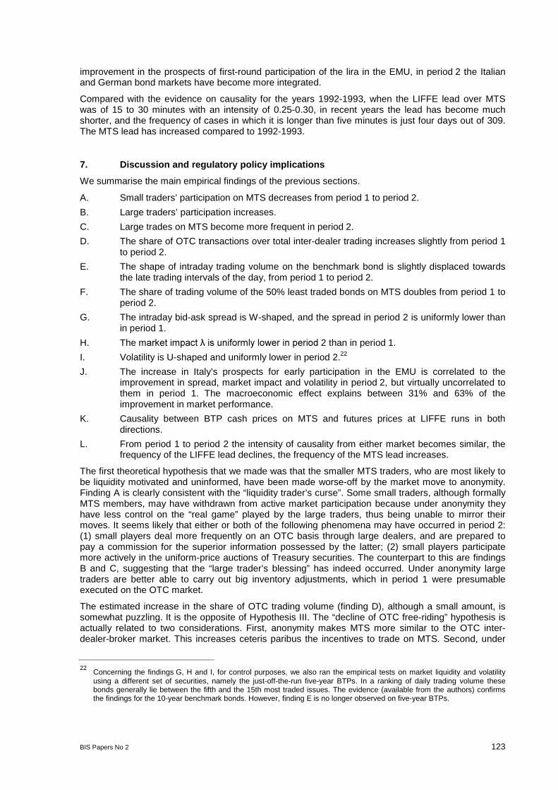
BIS Papers No 2 123
improvement in the prospects of first-round participation of the lira in the EMU, in period 2 the Italianand German bond markets have become more integrated.
Compared with the evidence on causality for the years 1992-1993, when the LIFFE lead over MTSwas of 15 to 30 minutes with an intensity of 0.25-0.30, in recent years the lead has become muchshorter, and the frequency of cases in which it is longer than five minutes is just four days out of 309.The MTS lead has increased compared to 1992-1993.
7. Discussion and regulatory policy implications
We summarise the main empirical findings of the previous sections.
A. Small traders’ participation on MTS decreases from period 1 to period 2.
B. Large traders’ participation increases.
C. Large trades on MTS become more frequent in period 2.
D. The share of OTC transactions over total inter-dealer trading increases slightly from period 1to period 2.
E. The shape of intraday trading volume on the benchmark bond is slightly displaced towardsthe late trading intervals of the day, from period 1 to period 2.
F. The share of trading volume of the 50% least traded bonds on MTS doubles from period 1 toperiod 2.
G. The intraday bid-ask spread is W-shaped, and the spread in period 2 is uniformly lower thanin period 1.
H. The m 2 than in period 1.
I. Volatility is U-shaped and uniformly lower in period 2.22
J. The increase in Italy’s prospects for early participation in the EMU is correlated to theimprovement in spread, market impact and volatility in period 2, but virtually uncorrelated tothem in period 1. The macroeconomic effect explains between 31% and 63% of theimprovement in market performance.
K. Causality between BTP cash prices on MTS and futures prices at LIFFE runs in bothdirections.
L. From period 1 to period 2 the intensity of causality from either market becomes similar, thefrequency of the LIFFE lead declines, the frequency of the MTS lead increases.
The first theoretical hypothesis that we made was that the smaller MTS traders, who are most likely tobe liquidity motivated and uninformed, have been made worse-off by the market move to anonymity.Finding A is clearly consistent with the “liquidity trader’s curse”. Some small traders, although formallyMTS members, may have withdrawn from active market participation because under anonymity theyhave less control on the “real game” played by the large traders, thus being unable to mirror theirmoves. It seems likely that either or both of the following phenomena may have occurred in period 2:(1) small players deal more frequently on an OTC basis through large dealers, and are prepared topay a commission for the superior information possessed by the latter; (2) small players participatemore actively in the uniform-price auctions of Treasury securities. The counterpart to this are findingsB and C, suggesting that the “large trader’s blessing” has indeed occurred. Under anonymity largetraders are better able to carry out big inventory adjustments, which in period 1 were presumableexecuted on the OTC market.
The estimated increase in the share of OTC trading volume (finding D), although a small amount, issomewhat puzzling. It is the opposite of Hypothesis III. The “decline of OTC free-riding” hypothesis isactually related to two considerations. First, anonymity makes MTS more similar to the OTC inter-dealer-broker market. This increases ceteris paribus the incentives to trade on MTS. Second, under
22Concerning the findings G, H and I, for control purposes, we also ran the empirical tests on market liquidity and volatilityusing a different set of securities, namely the just-off-the-run five-year BTPs. In a ranking of daily trading volume thesebonds generally lie between the fifth and the 15th most traded issues. The evidence (available from the authors) confirmsthe findings for the 10-year benchmark bonds. However, finding E is no longer observed on five-year BTPs.
124 BIS Papers No 2
anonymity it becomes more difficult for the OTC market to free-ride on price and order-flow informationprovided by MTS. This phenomenon may cause an increase in trading cost on the OTC market, andmay induce some dealers to trade directly on MTS. Are there any other reasons for the observedincrease in OTC turnover? It is possible that the OTC inter-dealer brokers have reacted to the 1997MTS shift, which increased competition between the two markets, by reducing spreads. We note aninteresting example concerning competition between the OTC market and MTS. Cantor Fitzgerald,one of the major brokers trading Italian bonds from London, had often used MTS through anintermediary in the past; at the end of 1997, it applied for membership with MTS and in May 1998 itstarted trading large volumes directly on the Italian market. Since MTS prices reflect a morehomogeneous market set-up, it is now conceivable that they can be straightforwardly applied to OTCtransactions. If this is so, then OTC free-riding on MTS might have even increased after the MTSswitch.
The fourth theoretical prediction that we investigated is the waiting game hypothesis of Foster andViswanathan. Finding E is consistent with this hypothesis: under anonymity the order flow informationof MTS has become less useful to dealers, and they tend to wait longer in order to extract moreinformation. There is a further reason for the slight displacement of the intraday profile of tradingvolume in period 2. During our sample period the Italian market has become increasingly integratedwith the other major financial markets. Among these, the US market is an important source ofinformation and it has been a growing source of investment into the Italian market. Hence, theinformation and orders that start arriving on MTS from 14:30 onward, ie from the opening of the USmarket and the release time of most US macroeconomic indicators, have increased over time, and thisclearly contributes to the observed shift in intraday trading volume on MTS.
Findings F to L represent in our opinion impressive evidence on the improvement in the performanceof MTS in recent years. In interpreting these results, we face an attribution problem. As we arguedearlier on, two distinct factors may have played a role, namely the switch to anonymity, a one-timeevent that took place in the middle of 1997, and the steady progress of public finance of 1996-1997.We tried to distinguish between these two factors, and obtained results that show that themicroeconomic effect amounts for 31 to 63% of the variation in the market performance variables. Inthe case of the two cost measures, the microeconomic effect is more important. In the case ofvolatility, the macroeconomic effect takes first place. This is not surprising, since market volatility maybe expected to be more sensitive to macroeconomic conditions than trading costs.
An additional factor that may have played a role is the listing to repo contracts on MTS starting inDecember 1997. Repo contracts on Treasury bonds have been traded among dealers on the OTCmarket for long before that date. However, cash traders greatly benefited from the inception of repotrading directly on MTS, through a reduction in the cost of setting up short positions. This may helpexplain why the speed of price discovery on MTS has increased with respect to the futures market(findings K and L).
From a regulatory point of view, the evidence presented in this paper has several implications. Thefirst implication is domestic. The move to anonymity has furthered the reform process of the Treasurybond market that the Italian regulatory authorities initiated in 1994 (see the Appendix table). Thisreform was aimed at restoring the competitive role of MTS with respect to the OTC market, by openingup the former to foreign investors, lowering transaction costs and promoting competition amongdealers. Since 1994 MTS has greatly increased efficiency and turnover relative to the OTC market. Aswe have shown, the 1997 shift helped to enhance this competition, affording higher levels of welfarefor those who invest in Italian Treasury bonds. The improvement of the secondary market should alsohave benefited the issuer, through a reduction in the cost of debt servicing. We conclude that the 1997innovation on MTS has proved successful.
The second regulatory implication follows from the first one. Looking at the Italian Treasury bondmarket from a more general perspective, we note that the market has made a remarkable progress injust one decade, from an opaque, lowly liquid market with negligible foreign participation to a highlytransparent and liquid market with a large participation of international investors. This progress hasbeen similar in nature to developments in other industrialised countries, but in the Italian case it hasbeen more intense. To this extent, MTS has played a key role. The ideas that have underlain the MTSinception and development have proved successful in the medium term. These ideas are: (1) fullautomation of the trading mechanism; (2) transparency; (3) large participation; (4) inside and outsidecompetition. We believe that the experience of MTS may be useful for those emerging countrieswishing to establish a liquid and efficient financial market in a relatively short time horizon.
BIS Papers No 2 125
In 1998 the market was fully privatised. A major development took place in September 1998, namelythe listing of a eurolira 10-year bond issued by the European Investment Bank and of a large group ofGerman government bonds.23 The listing of sovereign bonds from other countries is also planned. Inthe perspective of EMU, it has been argued that the likely integration of the European bond marketsmight imply either a strong cooperation among sovereign issuers, or a “race to benchmark status”(McCauley and White 1997). In both cases, the role of each country’s government bonds within theEuropean market will be positively affected by the liquidity conditions of the domestic market and bythe availability of the securities in the portfolios of international investors, even more than by thecreditworthiness of the issuer. In this view, the improvement in the liquidity of MTS, along with thedecision by the Italian Treasury to convert all outstanding debt in euros on 1 January 1999, places theItalian issues in a strong position among the partner countries’ issues.
8. Conclusion
We analysed a change in the organisation of the electronic inter-dealer market for Italian Treasurybonds known as MTS, namely the shift to the anonymity of quotes in July 1997. The implications ofthis event were investigated in the light of market microstructure theory and from a public welfareperspective. We employed an extensive data-set which includes all transactions carried out on MTSwith the identity of the traders, in the period from September 1996 to May 1998. In addition, we usedintraday prices for the BTP futures contract traded at LIFFE and for a set of financial instruments thatmay be viewed as explanatory variables for the dynamics of BTP prices. Our evidence supports thehypothesis that the decrease in transparency makes liquidity traders worse-off, whereaslarge/informed traders find it less costly to execute block trades. The evidence is also consistent withthe “waiting game” hypothesis of Foster and Viswanathan (1996) on intraday trading: underanonymity, traders tend to delay their trades in an attempt to acquire information through the orderflow. From a public welfare perspective, our results indicate that the move to anonymity has beenaccompanied by an increase in market liquidity and by a reduction in volatility, a phenomenon that isalso partly explained by the growth in Italy’s prospects for early participation in the EMU. The speed ofinformation aggregation on MTS increases, as shown by an improvement of the MTS lead over thefutures market. From a regulatory policy perspective our evidence suggests that, despite the welfareloss suffered by small traders, the move to anonymity has afforded an overall improvement in marketperformance. In this respect, the experience of MTS may be useful for the development of marketmechanisms in emerging countries. Finally, in a European perspective, the current organisation andperformance of MTS place the market in a competitive position compared to other cash markets forgovernment bonds, and may contribute to a closer integration of these markets under the EMU.
23Contracts on these bonds are cleared and settled through international depository entities (Euroclear and Cedel).
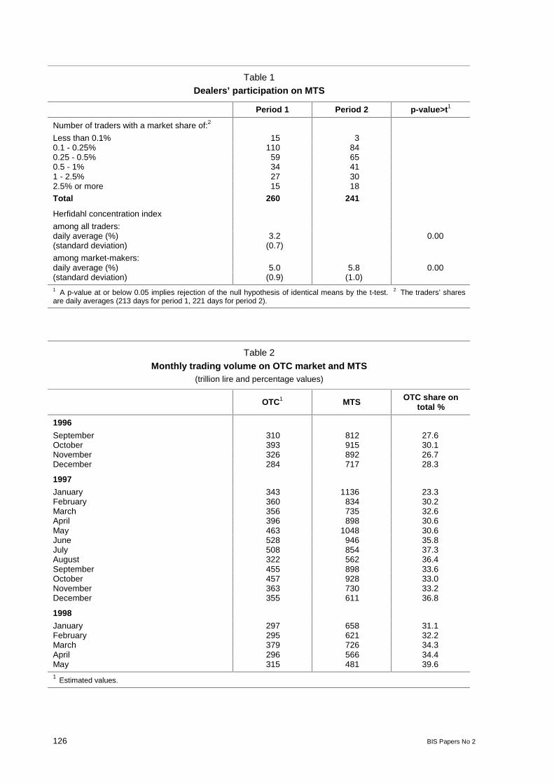
126 BIS Papers No 2
Table 1Dealers’ participation on MTS
Period 1 Period 2 p-value>t1
Number of traders with a market share of:2
Less than 0.1% 15 30.1 - 0.25% 110 840.25 - 0.5% 59 650.5 - 1% 34 411 - 2.5% 27 302.5% or more 15 18
Total 260 241
Herfidahl concentration index
among all traders:daily average (%) 3.2 0.00(standard deviation) (0.7)
among market-makers:daily average (%) 5.0 5.8 0.00(standard deviation) (0.9) (1.0)1 A p-value at or below 0.05 implies rejection of the null hypothesis of identical means by the t-test. 2 The traders’ sharesare daily averages (213 days for period 1, 221 days for period 2).
Table 2
Monthly trading volume on OTC market and MTS(trillion lire and percentage values)
OTC1 MTS OTC share ontotal %
1996
September 310 812 27.6October 393 915 30.1November 326 892 26.7December 284 717 28.3
1997
January 343 1136 23.3February 360 834 30.2March 356 735 32.6April 396 898 30.6May 463 1048 30.6June 528 946 35.8July 508 854 37.3August 322 562 36.4September 455 898 33.6October 457 928 33.0November 363 730 33.2December 355 611 36.8
1998
January 297 658 31.1February 295 621 32.2March 379 726 34.3April 296 566 34.4May 315 481 39.61 Estimated values.
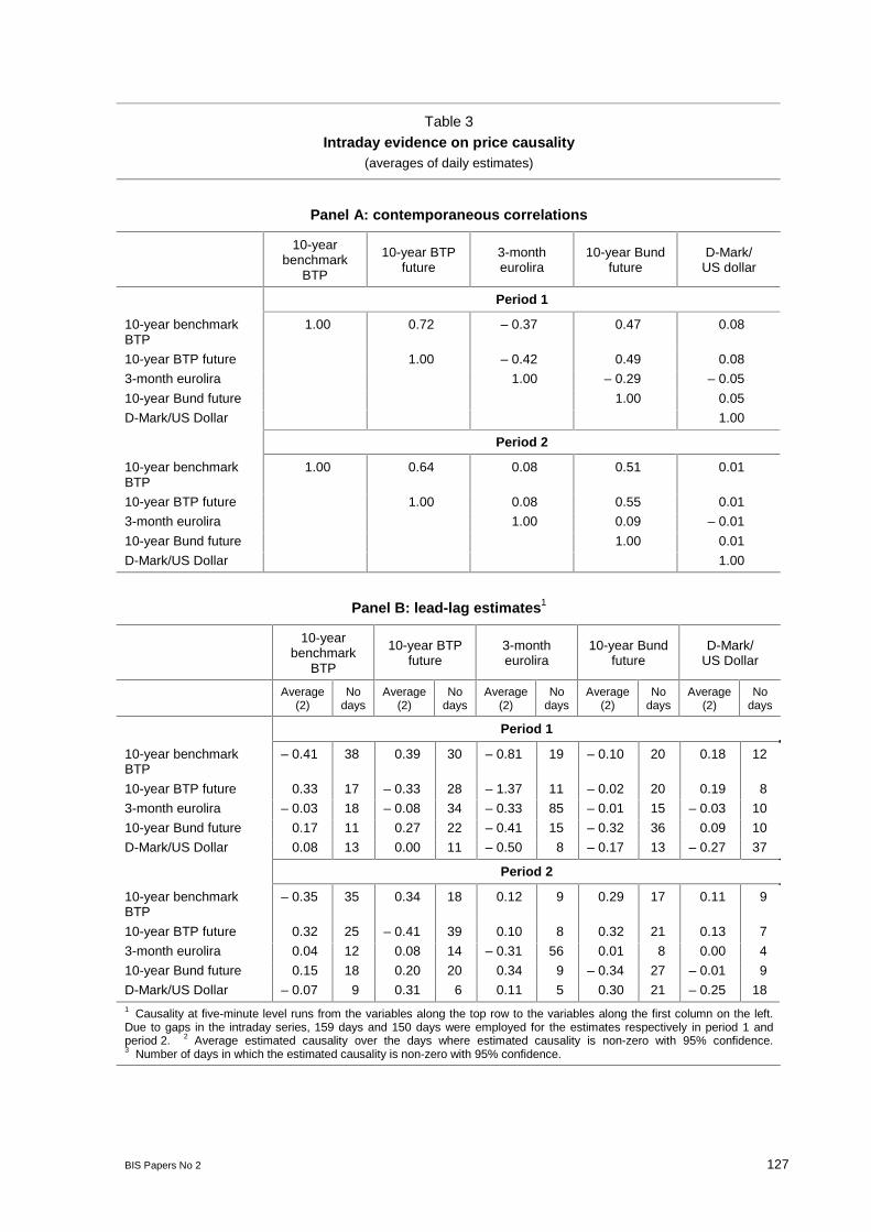
BIS Papers No 2 127
Table 3Intraday evidence on price causality
(averages of daily estimates)
Panel A: contemporaneous correlations
10-yearbenchmark
BTP
10-year BTPfuture
3-montheurolira
10-year Bundfuture
D-Mark/US dollar
Period 1
10-year benchmarkBTP
1.00 0.72 – 0.37 0.47 0.08
10-year BTP future 1.00 – 0.42 0.49 0.08
3-month eurolira 1.00 – 0.29 – 0.05
10-year Bund future 1.00 0.05
D-Mark/US Dollar 1.00
Period 2
10-year benchmarkBTP
1.00 0.64 0.08 0.51 0.01
10-year BTP future 1.00 0.08 0.55 0.01
3-month eurolira 1.00 0.09 – 0.01
10-year Bund future 1.00 0.01
D-Mark/US Dollar 1.00
Panel B: lead-lag estimates1
10-yearbenchmark
BTP
10-year BTPfuture
3-montheurolira
10-year Bundfuture
D-Mark/US Dollar
Average(2)
Nodays
Average(2)
Nodays
Average(2)
Nodays
Average(2)
Nodays
Average(2)
Nodays
Period 1
10-year benchmarkBTP
– 0.41 38 0.39 30 – 0.81 19 – 0.10 20 0.18 12
10-year BTP future 0.33 17 – 0.33 28 – 1.37 11 – 0.02 20 0.19 8
3-month eurolira – 0.03 18 – 0.08 34 – 0.33 85 – 0.01 15 – 0.03 10
10-year Bund future 0.17 11 0.27 22 – 0.41 15 – 0.32 36 0.09 10
D-Mark/US Dollar 0.08 13 0.00 11 – 0.50 8 – 0.17 13 – 0.27 37
Period 2
10-year benchmarkBTP
– 0.35 35 0.34 18 0.12 9 0.29 17 0.11 9
10-year BTP future 0.32 25 – 0.41 39 0.10 8 0.32 21 0.13 7
3-month eurolira 0.04 12 0.08 14 – 0.31 56 0.01 8 0.00 4
10-year Bund future 0.15 18 0.20 20 0.34 9 – 0.34 27 – 0.01 9
D-Mark/US Dollar – 0.07 9 0.31 6 0.11 5 0.30 21 – 0.25 181 Causality at five-minute level runs from the variables along the top row to the variables along the first column on the left.Due to gaps in the intraday series, 159 days and 150 days were employed for the estimates respectively in period 1 andperiod 2. 2 Average estimated causality over the days where estimated causality is non-zero with 95% confidence.3 Number of days in which the estimated causality is non-zero with 95% confidence.
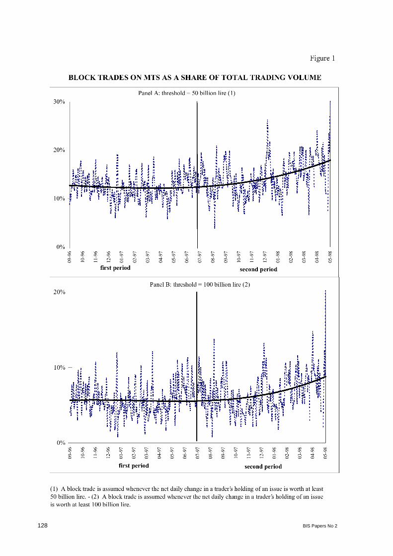
128 BIS Papers No 2
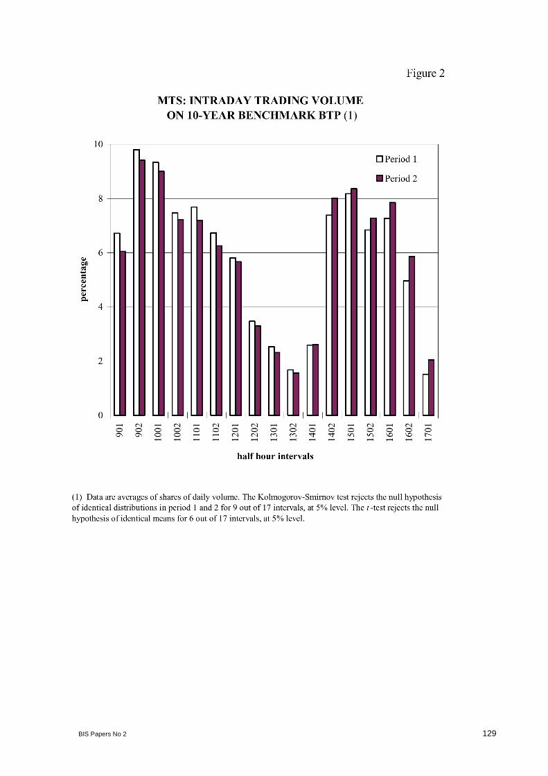
BIS Papers No 2 129
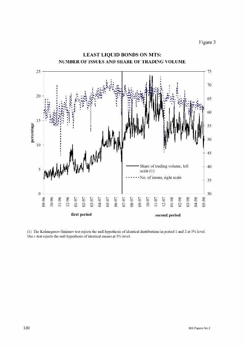
130 BIS Papers No 2
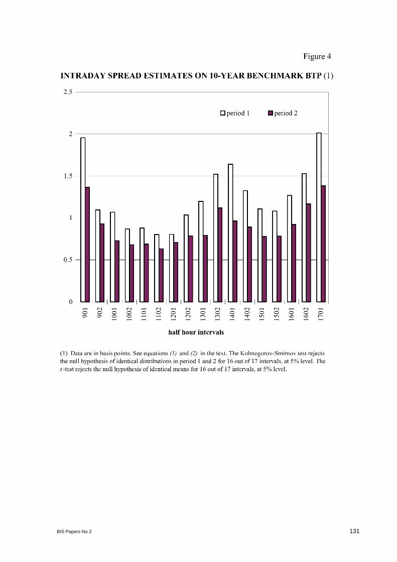
BIS Papers No 2 131
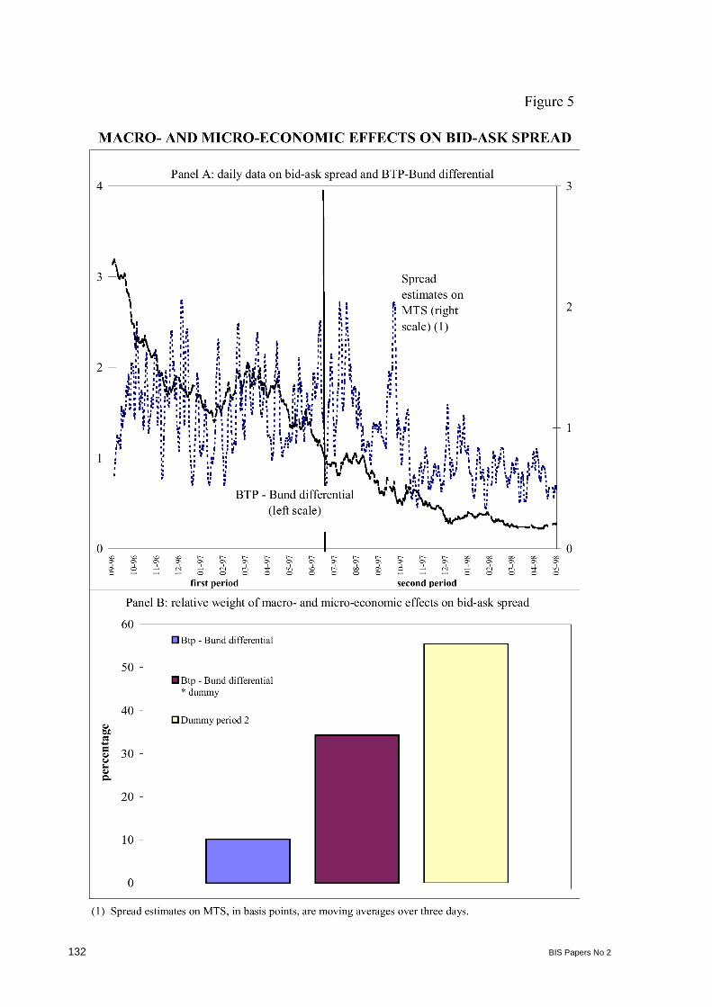
132 BIS Papers No 2
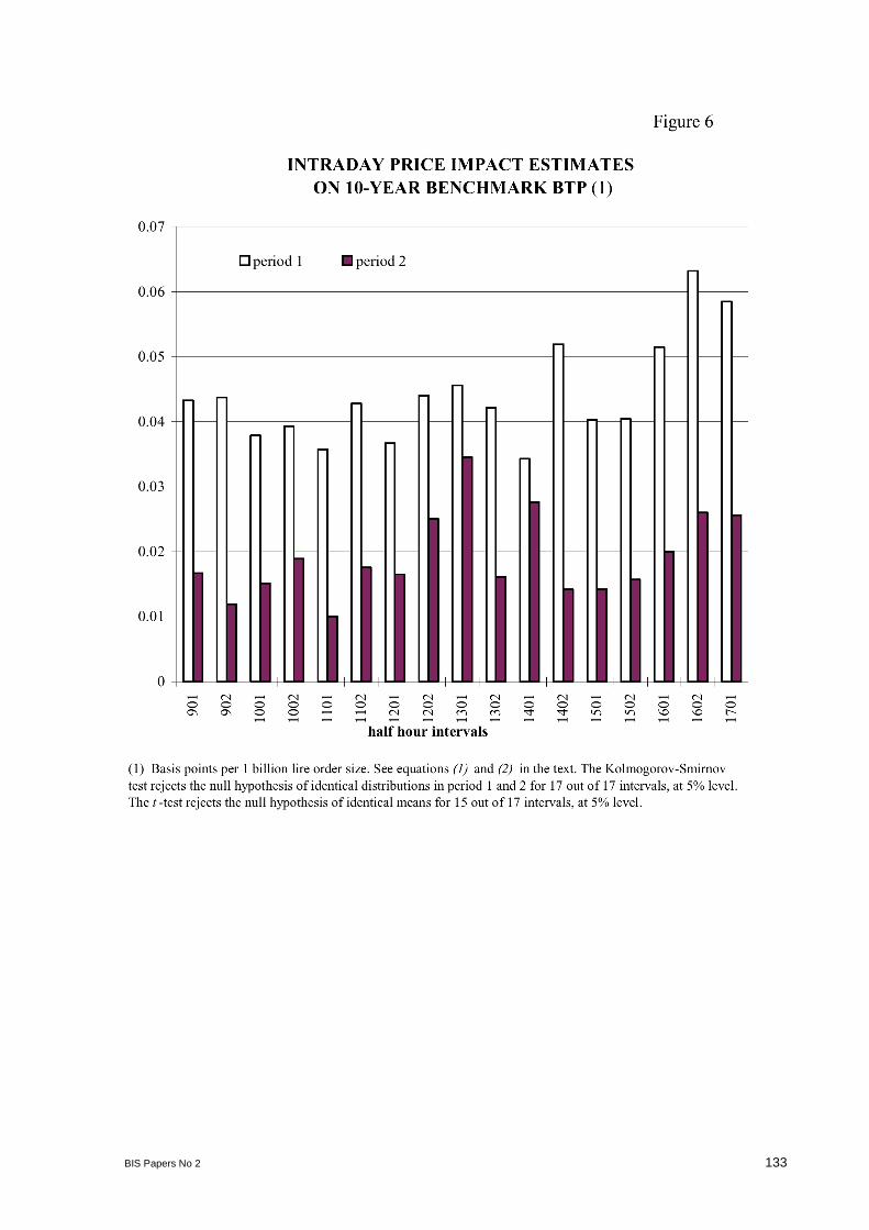
BIS Papers No 2 133
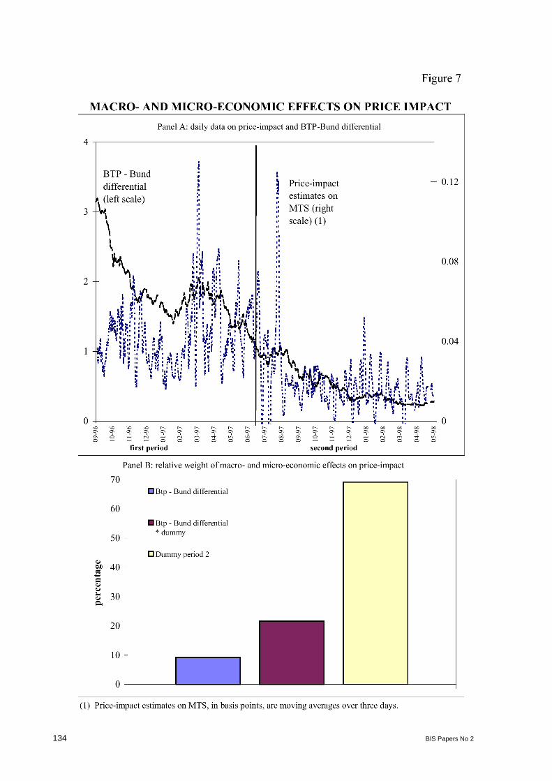
134 BIS Papers No 2
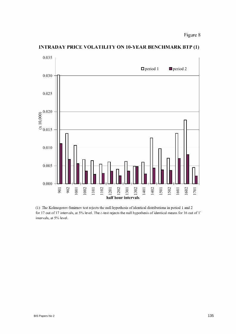
BIS Papers No 2 135
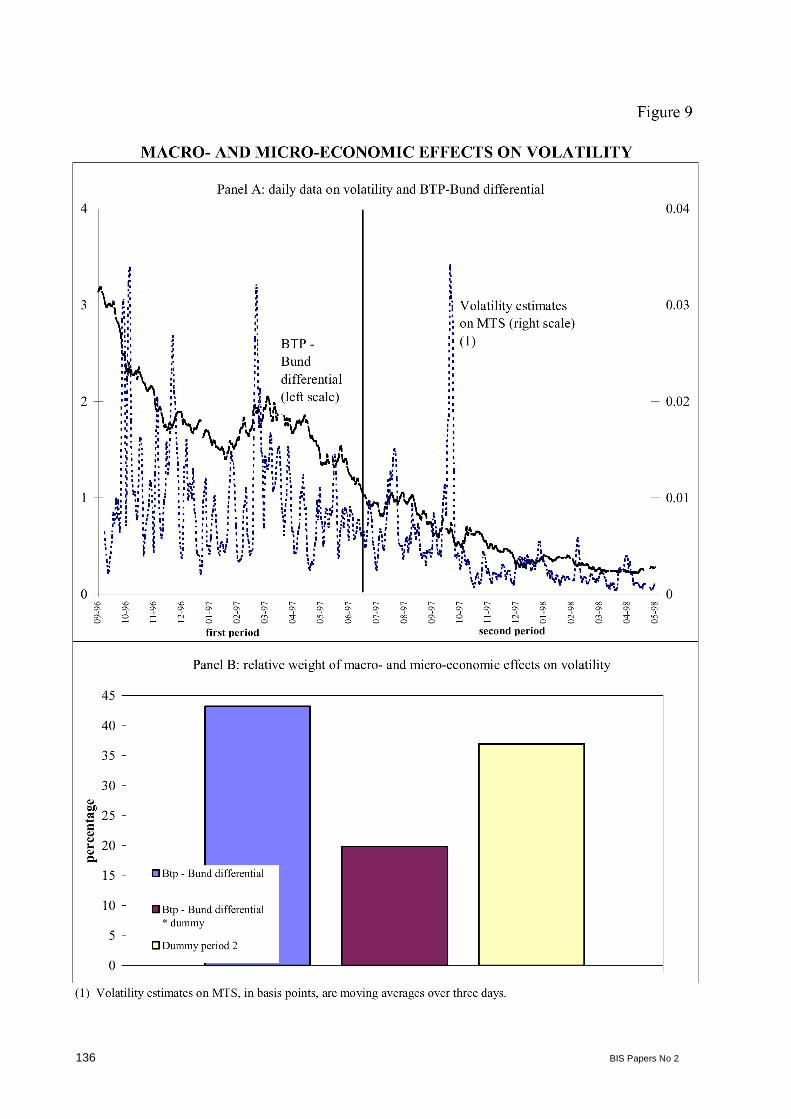
136 BIS Papers No 2

BIS Papers No 2 137
Appendix
The development of the Italian GovernmentBond Market in the last decade
Year International integration Changes in marketmicrostructure New instruments
1998 Liberalisation of capital flows(partial)
Inception of MTS
Start of regular reopenings ofTreasury auctions
Floor to bid prices abolished forT-bills, uniform price auctionintroduced for other bonds.
1990 Liberalisation of capital flows(full)
Real-time securities transferral atthe central depository Bancad’Italia
1991 10-year BTP futures at LIFFE(London)
1992 Inception of the Italian futuresmarket (MIF)
1993 First US$ global bond issue bythe Republic of Italy.Prohibition of direct financing ofthe Treasury by the Bancad’Italia
First insurance of 30-year BTPs
1994 Reform of MTS Treasury starts publishingtimetable of auctions
Electronic bid submission atauctions
Reserved reopenings for“specialists in governmentactivities”
Continuous trading on MOT, theelectronic retail market
1995 First issuance of CTZs (two-yearzero coupon bonds)
CCT indexation fully matchedwith contemporaneous six-monthbills
1996 EU investment Service Directivemade effective
1997 Withholding tax abolished forforeign investors
Remote access to MTS forforeign primary dealers
Monitoring functions to the MTSmanagement board
Treasury bond repo trading startson MTS
1998 First ad hoc reopenings ofTreasury auctions
Book-entry system for all newtreasury issues
Coupon-strips traded on MTS

138 BIS Papers No 2
References
Angeloni, I, F Drudi and G Majnoni (1996): “Relazioni fra prezzi a pronti e futures sui BTP decennali:un’ analisi su dati infragiornalieri”, Banca d’Italia, Temi di discussione, No 283.
Banca d’Italia (1994): Economic Bulletin, No 18, pp 52-53.
Dattels, P (1995): “The Microstructure of Government Securities Markets”, IMF, Working Paper,No 95/117.
Domowitz I (1990): “The Mechanics of Automated Trade Execution”, Journal of FinancialIntermediation, No 1, pp 167-94.
Fama, E F (1970): “Efficient Capital Markets: A review of Theory and Empirical Work”, Journal ofFinance, Vol 25, No 2, pp 383-417.
Fleming, M J and E M Remolona (1997): “Price Formation and Liquidity in the US Treasury Market:Evidence from Intraday Patterns Around Announcements”, Federal Reserve Bank of New York, StaffReports, No 27.
Foster, M M and T J George (1992): “Anonymity in Securities Markets”, Journal of FinancialIntermediation, Vol 2, pp 168-206.
Foster, F D and S Viswanathan (1993): “ Variations in Trading Volume, Return Volatility and TradingCosts: Evidence on recent Price Formation Models”, Journal of Finance, Vol 48, No 1, pp 187-211.
Foster F D and S Viswanathan (1996): “Strategic Trading When Agents Forecast the Forecasts ofOthers”, Journal of Finance, Vol 51, No 4, pp 1437-78.
Franks J and S M Schaefer (1995): “Equity Market Transparency on the London Stock Exchange”,Bank of America Journal of Applied Corporate Finance, Vol 8, No 1, pp 70-77.
Grossman, S J (1988): “An Analysis of the Implications for Stock and Futures Price Volatility ofProgram Trading and Dynamic Hedging Strategies”, Journal of Business, Vol 61, pp 275-98.
Hasbrouck, J (1991): “Measuring the Information Content of Stock Trades”, Journal of Finance, Vol 46,No 1, pp 179-207.
Inoue, H (1999): “Summary of the questionnaire on the Structure of government securities markets -ECSC Study Group on Market Liquidity”, Bank of Japan, Working Paper.
Lyons, R K (1995): “Tests of Microstructural Hypothesis in the Foreign Exchange Market”, Journal ofFinancial Economics, Vol 39, pp 321-51.
Madhavan A (1995): “Consolidation, Fragmentation and the Disclosure of Trading Information, Reviewof Financial Studies, Vol 8, No 3, pp 579-603.
Madrigal, V (1996): “Non-fundamental Speculation”, Journal of Finance, Vol 51, No 2, pp 553-78.
McCauley R N and W R White (1997): “The Euro and European Financial Markets”, in T Krueger,P Masson and B Turtelboom (eds.), European Monetary Union and the International MonetarySystem, Washington DC, International Monetary Fund.
Miyanoya, A, H Inoue and H Higo (1997): “Market liquidity of the Japanese Government SecuritiesMarket”, Bank of Japan, Working Paper.
Muranaga J and T Shimizu (1997): “Market Microstructure and Market Liquidity”, Institute for Monetaryand Economic Studies, Bank of Japan, Working Paper.
Naik, N, A Neuberger and S Viswanathan (1994): “Disclosure Regulation in Competitive DealershipMarkets: An Analysis of the London Stock Exchange”, London Business School, Institute of Financeand Accounting, Working Paper, No 193.
O’Hara M (1995): “Market Microstructure Theory”, Cambridge MA, Blackwell.
Pagano, M and A Röell (1996): “Transparency and Liquidity: A comparison of Auction and DealerMarkets with Informed Trading”, Journal of Finance, Vol 51, No 2, pp 579-612.
Proudman J (1995): “The microstructure of the UK gilt market”, Bank of England, Working Paper,No 38.

BIS Papers No 2 139
Santini C (1997): “Public Debt Management and Monetary Control in Italy”, in V Sundarajan, P Dattelsand H J Blommestein (eds), “Coordinating Public Debt and Monetary Management: Institutional andOperational Arrangements”, Washington DC, International Monetary Fund.
Scalia, A (1998a): “Periodic information asymmetry and intraday market behaviour: an empiricalanalysis”, European Finance Review, Vol 1, No 3, pp 307-35.
Scalia, A (1998b): “Information Transmission and Causality in the Italian Treasury Bond Market”,Journal of Empirical Finance, Vol 5, No 4, pp 361-84.
Recently Published “TEMI”24
No 334 - “La politica fiscale nei paesi dell’Unione europea negli anni novanta”, by P Caselli andR Rinaldi (July 1998).
No 335 - “Signaling Fiscal Regime Sustainability”, by F Drudi and A Prati (September 1998).
No 336 - “Fiscal Consolidations under Fixed Exchange Rates”, by P Caselli (October 1998).
No 337 - “Investimenti diretti all’estero e commercio: complementi o sostituti?”, by A Mori and V Rolli(October 1998).
No 338 - “Nonlinear VAR: Some Theory and an Application to US GNP and Unemployment”, byF Altissimo and G L Violante (October 1998).
No 339 - “The Probability Density Function of interest Rates implied in the Price of Options”, byF Fornari and R Violi (October 1998).
No 340 - “Heterogeneous ‘Credit Channels’ and Optimal Monetary Policy in a Monetary Union”, byL Gambacorta (October 1998).
No 341 - “Enemy of None but a Common Friend of All?” An International Perspective on the Lender-of-Last-Resort Function, by C Giannini (December 1998).
No 342 - “Energy Consumption, Survey Data and the prediction of Industrial Production in Italy”, byD J Marchetti and G Parigi (December 1998).
No 343 - “What Caused the Asian Currency and Financial Crisis?”, by G Corsetti, P Pesenti andN Roubini (December 1998).
No 344 - “Investment and the Exchange Rate”, by F Nucci and A F Pozzolo (December 1998).
No 345 - “Reallocation and Learning over the Business Cycle”, by F Schivardi (December 1998).
No 346 - “Una ricostruzione omegenea di dati regionali: contri economici e reddito disponibile dellefamiglie 1970-1995”, by P Berrettoni, R Delogu, C Pappalardo and P Piselli (February 1999).
No 347 - “Industrial Districts and Local Banks: Do the Twins ever Meet?”, by A Baffigi, M Pagnini andF Quintilliani (March 1999).
No 348 - “Orari di lavoro atipici in Italia: un’analisi attraverso l’Indagine dell’uso del tempo dell’Istat”, byR Torrini (March 1999).
No 349 - “Gli effetti economici del nuovo regime di tassazione delle rendite finanziarie”, by R Cesari(March 1999).
No 350 - “The Distribution of Personal Income in Post-War Italy: Source Description, Data Quality andthe Time Pattern of Income Inequality”, by A Brandolini (April 1999).
No 351 - “Median Voter Preferences, Central Bank Independence and Conservatism”, by F Lippi (April1999).
24Request for copies should be sent to: Banca d’Italia - Servizio Studi - Divisione Biblioteca e pubblicazione - Via Nazionale,91 - 00184 Rome (fax 0039 06 47922059).

140 BIS Papers No 2
No 352 - “Errori e omissioni nella bilancia dei pagamenti: esportazioni di capitali e apertura finanziariadell’Italia”, by M Committeri (June 1999).
No 353 - “Is there an equity premium puzzle in Italy? A look at asset returns, consumption andfinancial structure data over the last century”, by F Panetta and R Violi (June 1999).
No 354 - “How deep are the deep parameters?”, by F Altissimo, S Siviero and D Terlizzese (June1999).
No 355 - “The Economic policy of Fiscal consolidations: The European experience”, by A Zaghini(June 1999).
No 356 - “What is the Optimal Institutional Arrangement for a Monetary Union?”, by L Gambacorta(June 1999).
No 357 - “Are Model-Based inflation forecasts used in Monetary policymaking? A case study”, byS Siviero, D Terlizzese and I Visco (September 1999).
No 358 - “The Impact of News on the exchange rate of the Lira and long-term interest rates”, byF Fornari, C Monticelli, M Pericoli and M Tivegna (October 1999).
BIS Papers No 2 141
Comments on “Does market transparency matter? A case study”by A Scalia and V Vacca
Agnes Van den Berge, Banque Nationale de Belgique
The paper “Does market transparency matter? A case study” discusses the influence of a decrease intransparency resulting from anonymous trading on the Italian MTS electronic trading system, adealer system. The study supports the theoretical evidence that a decrease in transparency makesliquidity traders (those traders who know only the price process) worse off whereas large informedtraders (those who know more about fundamental asset values than others) are better off becausethey can better exploit their private information.
The study indicates that the decrease in transparency was associated with an increase in marketliquidity, a reduction in trading costs and in price volatility and with an increase in market efficiency,defined as the degree to which prices fully reflect all available information.
Market transparency is usually defined as “the ability of market participants to observe theinformation on the trading process”. However, transparency has many dimensions because a markethas many kinds of participants and many types of information. The information can either be public(available to all market participants eg publicly announced statistics) or private (not available to allmarket participants and including both inside information about fundamentals and information on orderflows or customer behaviour).
The study discusses the impact of a change in transparency of the Italian MTS resulting from a moveto anonymity where the names of the market makers who post bid and ask quotes were no morerevealed. In the study the change of transparency only treated one type of information in a specificmarket microstructure namely a quote-driven dealer market.
Academic findings are far from conclusive regarding the relationship between the level of transparencyand the liquidity of bond markets. But in a dealer market, such as MTS, which is yet highly transparent,decreasing certain kinds of transparency can sometimes be beneficial. However, this may not lead togeneral conclusions about the relationship between transparency and liquidity which the study doesnot but I would like to stress the importance of this for the audience.
Transparency of market information has two aspects namely pre-trade quotes and post-tradeinformation on prices/quantities actually transacted.
An early disclosure of information on specific orders, including the names of the dealers posting theorders linked to the size of these orders, does indeed appear counterproductive for the liquidity ofdealer markets because of the risk of disclosing the movements in the market-maker’s books. A tooimmediate (eg real-time) dissemination of this information to the market may reduce the incentive fordealers to make markets. Other elements of the pre-trade price transparency, such as the publicationof aggregated volumes by limits, are beneficial to the liquidity of the market.
Where the study finds that the reduction of pre-trade transparency (move to anonymity) has hadpositive effects on the liquidity of the market, it does not give any indication of the effects of adisclosure of more detailed information after trade execution (post-trade transparency). Post-tradetransparency makes markets fairer but it becomes harder for market makers to unwind positionsquietly as prices would be more responsive to trades. Therefore it also may reduce liquidity. In adealer market, the right balance has to be found between the level of transparency and the interests ofthe involved market-makers.
After these general observations on the interaction between transparency and liquidity, the reading ofthe paper leads us to three, more specific remarks and comments.
Firstly, the data used in the empirical analysis are the transactions in the period from September 1996to end May 1998. It is mentioned in the study that macroeconomic effects have had a very importantimpact on the market performance. It has to be stressed that during the second part of the periodunder review, financial markets in Europe and thus also government bond markets were largelyinfluenced by the impending introduction of the euro and the gradual emergence of pan-Europeanfinancial markets. This was certainly the case in Italy.

142 BIS Papers No 2
Secondly, in accordance with the theoretical models, the decrease in transparency caused a reductionin the number of small traders. Even if the number of the larger traders increased, the overall numberof market participants declined. In a context of bond markets where a limited number of globalmarket-makers captures a growing size of the order flow from institutional and retail investors, theincreasing market concentration should be a matter of concern because of its negative impact on theliquidity of the market. This applies even more to smaller markets where the number of marketparticipants often is limited.
Finally, the empirical evidence shows that the reduction in transparency was accompanied by adecline in volatility but that the microeconomic effect (introduction of pre-trade anonymity) explainedonly 37 per cent of this evolution. Should the anonymity move have been taken today, then it seemsdoubtful that there would be a significant impact on volatility. At present, the most important dealers inthe eurozone automatically derive their posted prices from a set of (exogenous) parameters like thecorresponding yield of the Bund-future.
Let me now give a few remarks on the Belgian experience with electronic trading platforms forgovernment bonds.
MTS Belgium has been operational since 5 May 2000. It introduced the Italian model and starteddirectly with anonymous trading. At present, the dealer quotes and the order book are only available tomarket participants. Discussions are under way with information vendors to allow them to disseminatemarket information on their screens (with a certain delay) which will improve the market transparency.
All fixed rate OLO bonds with a remaining life to maturity of over 1.25 years are currently traded onMTS Belgium (16 bonds), representing a total outstanding amount of 138 billion euro.
For the time being, 16 primary dealers in Belgian government bonds and 1 market maker have accessto the system. Market access will further be extended to domestic and foreign financial intermediariesin the capacity of price taker.
Five Belgian bonds are currently traded on EuroMTS representing a total outstanding amount of48 billion euro. The first introduction took place on 9 September 1999.
Since 3 July 2000, twenty Belgian bonds are traded on Broker-Tec.
The market share of electronic trading can be estimated at roughly one third of the total turnover ofpurchase/sale transactions in OLO bonds. Turnover in OLO bonds on Broker Tec has been marginalsince its launch.
The electronic trading of Belgian government bonds, especially their introduction on EuroMTS followedby the launch of a domestic MTS, has resulted in lower transaction costs in terms of fees andbid/ask-spreads compared to the OTC market. This is also due to the straight through processingfacilities MTS provides. As such, it has improved the liquidity of the secondary market. Furtherimprovements in market transparency and an increasing number of market participants should give anadditional boost to market liquidity in the future.
Conclusions
If conceptually a totally transparent market should be favourable for the liquidity of bond markets,practically in a dealer market, a compromise has to be found between the level of transparency andthe involvement of the market-makers who expect a return on the capital invested in the marketmaking activity. In Italy, where a reduction in market transparency (move to anonymity) has led to animprovement of market liquidity, the MTS market seemed initially “too transparent”. By contrast, theintroduction of electronic trading in Belgium increased market transparency which, together with lowertransaction costs, improved market liquidity.
BIS Papers No 2 143
Comments on “Does market transparency matter? A case study”by Antonio Scalia and Valeri Vacca
Peter Rappoport, JP Morgan
The asymmetric information view of markets points out that traders’ behaviour will be driven in specificways by the environment in which they trade. It predicts, for example, that bid-offer spreads should bewider, the greater is the chance that a market maker has to trade with informed individuals, and thatliquidity may be lowered by transparent trading, because transparency limits the return to market-making. Any theory that can successfully predict liquidity conditions would very quickly find a place asa market staple.
To test such a theory, a controlled experiment would be the best, and one actually appears to havebeen provided by the move of the MTS system to anonymous trading in mid-1997. The authors arguecogently that this change in rules would have four principal observable implications. Some are relatedto the shift in the “balance of power” towards large market specialists, to the detriment of MTS “liquiditytraders”, and those in the OTC market who faced a reduced flow of information. Others follow from thechange in the optimal trading strategy under the new rules.
The authors provide a clear and erudite exposition of an impressive battery of tests of thesehypotheses. With one exception, they find that things moved in the predicted direction following theswitch to anonymous trading. As liquidity improved following the introduction of anonymous trading,they suggest that anonymity may be a desirable feature to incorporate into the design of new markets.
My interest in this paper is in where it leaves one on the broader questions related to liquidity I outlinedat the start. Should the paper’s evidence give one a new respect for the asymmetric informationdimension of market microstructure, or is there something else going on? Essentially, the question isnot so much one of whether the predicted directions of the responses to lower transparency areconfirmed. It is more a matter of whether the effects of the change are large, relative to the otherinfluences on the way markets trade. Here, things are less clear.
For example, the only hypothesis contradicted by the authors’ evidence is that the OTC market shouldhave suffered, because its ability to “free-ride” on information about sources of MTS flows wascurtailed. However, the authors cogently argue that there were other extenuating circumstances at thetime that could have led to the continued growth in the OTC share of the market. But then, how big arethese extenuating circumstances in other instances?
I have little doubt that asymmetric information considerations are present where prices are set bymarket makers. But at least in the bond world, it seems hard to believe they are dominant. The onlyinformation advantage that seems to be around in government bonds concerns not so much an insidetrack on fundamentals, such as interest rate policy or macroeconomic news, but knowledge of flows, iethat a big liquidity trade is imminent, from which profits can be made by “positioning ahead”. Here,there is no winner’s curse in having traded with the informed: the fundamental value of the securitiesbought (sold) has not necessarily fallen (risen). The only thing that has been missed is the opportunityto make life difficult for the trader who knows of the liquidity flows, and, thereby, to increase thechance of gaining some of the returns from the flows for oneself. Asymmetry of information may bemore important in equity markets, where information on individual stocks’ fundamentals can plausiblyflow slowly enough among market participants for market makers to worry about the winner’s curse.However, in corporate bond markets, which presumably dance to the same fundamentals tune asequity markets, inventory management appears, to me at least, to be a more pressing concern, and amore proximate determinant of bid-offer spreads.
The evidence presented by the paper does have something to offer on the importance of asymmetricinformation, but it is not very encouraging. As predicted by the theory, a move to lower transparencyshould lower the bid-offer spread. Figure 4 in the paper, reproduced below shows the bid-offer spreadduring half-hour periods in the trading day.
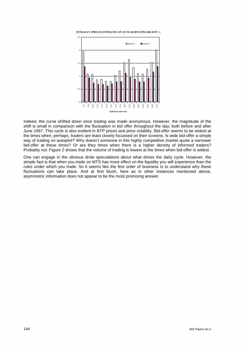
144 BIS Papers No 2
Indeed, the curve shifted down once trading was made anonymous. However, the magnitude of theshift is small in comparison with the fluctuation in bid offer throughout the day, both before and afterJune 1997. This cycle is also evident in BTP prices and price volatility. Bid-offer seems to be widest atthe times when, perhaps, traders are least closely focussed on their screens. Is wide bid-offer a simpleway of trading on autopilot? Why doesn’t someone in this highly competitive market quote a narrowerbid-offer at these times? Or are they times when there is a higher density of informed traders?Probably not: Figure 2 shows that the volume of trading is lowest at the times when bid-offer is widest.
One can engage in the obvious drole speculations about what drives the daily cycle. However, thesimple fact is that when you trade on MTS has more effect on the liquidity you will experience than therules under which you trade. So it seems like the first order of business is to understand why thesefluctuations can take place. And at first blush, here as in other instances mentioned above,asymmetric information does not appear to be the most promising answer.
BIS Papers No 2 147
Short introduction on the work of the Johnson-group
Eloy Lindeijer, De Nederlandsche Bank
Following the liquidity crisis of autumn 1998 the Committee on the Global Financial System formed aworking group to examine the events surrounding the market stresses that evolved during that period.Special focus was given to the suddenness of liquidity deterioration and mechanisms that contributedtowards the widespread withdrawal of risk taking. The group, which was chaired by Karen Johnson ofthe Federal Reserve Board, included representatives of central banks and monetary authorities fromG-10 countries and emerging markets. Market participants were interviewed in financial centres inEurope, Asia and the Americas to get a global perspective and the group assembled a large data seton key financial indicators to compare the events of end-1998 with previous episodes of marketturbulence.
With regard to the run up to the liquidity crisis the Johnson-group noted that risk spreads andvolatilities in G10 markets were on the low side of experience, particularly given the market turbulencein Asia during 1997 and 1998. One explanation put forward was the scale of resources devoted to riskarbitrage, driven by widespread emulation of relative value strategies pioneered by firms such asLTCM and the perception of risk free bets. This had helped reinforce linkages across markets,narrowing spreads and reducing volatilities in a way that reinforced macro-economic trends, such asdeclining capital market interest rates. This ‘overextention’ led to a severe market reaction, for whichRussia’s de facto default served as a trigger.
Market dislocation reached a peak during the recapitalisation of LTCM as worries about mass sales,risk concentration and above all systemic risk led to widespread risk withdrawal. Indicative of thesevere hedging pressures related to the unwinding of so-called carry trades was the 9% move inusd-japanese yen on October 7-8. In some niche products (such as Danish mortgage backedsecurities) arbitrageurs had built positions that amounted to multiples of typical daily market turnover,thus making it difficult to unwind positions without substantial market impact. In fixed-come marketsthis phenomenon led to an explosion of swap and credit spreads. 1998 also produced some of thelargest stock market declines for the decade, in some case just falling short of the 1987 crash.Volatility of bond and credit spreads, however, generally remained below the peaks experienced in1991 and 1994.
Compared with earlier episodes of market turbulence the Johnson-group concluded the autumn of1998 was an unusual, but not an extremely rare event. It demonstrated that the ‘abnormal’ returnsearned by relative value arbitrage players were in fact not risk free when viewed over a longer timespan. Policy makers concluded that some of the mechanisms that produce contagion and amplifymarket turbulence can be addressed by better risk management, capital and disclosure. Interestingly,some commentators argue the opposite case: that the response of policy makers may actuallycontribute towards greater herd behaviour in the future (triggered by disclosure of market sensitivedata) and has already resulted in more permanent reduction of market liquidity in the main markets, asmarket makers and speculators have withdrawn risk bearing capital. My personal inclination is toargue that liquidity has not deteriorated in global financial markets, but has returned to moresustainable levels subsequent to processes of deleveraging. With regard to herding it is important thatpolicy makers create an environment that makes it less likely that such flows create systemicconcerns. I would argue that disclosure and transparency increases the resilience of the financialsystem through greater market discipline.
A second important but not unrelated issue concerns the impact of technology on the functioning ofmarkets. The emergence of the e-commerce is impacting market liquidity today in ways that are notvery well understood. Competing electronic trading platforms may be contributing to a fragmentation ofliquidity in previously centralised markets. Alternatively new smart order routing systems may beproviding a single portal to all available pools of liquidity, effectively re-creating one central marketplace. The current state of liquidity of global financial markets may be an interesting issue for furtherdiscussion today, time permitting.
Let me conclude with one of the remaining imprints of the Johnson-study for my work as a centralbanker. Understanding the structure and functioning of markets is important, both form a monetarypolicy and systemic risk perspective. End-1998 some of the most visible manifestations of marketstress occurred in markets not always directly followed by central banks. As more risks become priced

148 BIS Papers No 2
in a world that is marked to market, central banks have realised the need to build up expertise outsidethe traditional realm of money and forex markets. Developments in swap, credit and equity marketsand the impact of e-commerce have become important and are therefore monitored on an on-goingbasis. The work programme of the CGFS is a good example of this.

BIS Papers No 2 149
Market liquidity under stress:observations from the FX market
Francis Breedon, Lehman Brothers
Given the thorough exposition of the theoretical aspects of liquidity given elsewhere in the conference,I will focus my remarks on a market perspective to these issues. First, outlining in general how periodsof market stress appear from an FX dealing floor, and second looking in detail at whether the eurocould be subject to such an event.
FX markets under stress
Market makers tend to identify two types of stress events in FX markets, the first involving highvolatility and high turnover the second high volatility and low turnover. In general, high volatility andhigh turnover events are good times for market makers, since they can achieve the seeminglycontradictory combination of keeping quoted spreads relatively narrow while substantially increasingtheir profit per trade. This is achieved through higher effective spreads whereby market makers find iteasier to “read” incoming trades and so quote accordingly. Examples of this type event include theperiodic 10 yen moves of dollar/yen, and the fallout for a developed country currency crisis. Althoughlarge trades are difficult to execute in such periods, liquidity in terms of the ability to execute a traderemains, the cost is that effective spreads are wide.
High volatility low turnover events are rarer and represent bad times for market makers. These usuallyoccur after a high volatility high turnover event but change in character as the market has lost two-wayinterest. Despite being able to read future trades, market makers are unable to make money as it isimpossible to lay off trades elsewhere. Therefore, these any trades have a disproportionate impact onprices and market makers find themselves on the wrong side of these moves. The reaction is to widenquoted spreads considerably or not quote at all. Although these event are rare, the aftermath of theAsian currency crisis supplied a few examples. In particular, the Indonesian Rupiah went through anextended period of low turnover and high volatility. Interestingly, this occurred once internationalinvestors had almost totally withdrawn from trading, while domestic investors still had a strong demandfor dollars.
From a policy-maker point of view it could be argued that high turnover high volatility events areunfortunate, but preferable to the low turnover variety. Certainly, the majority of currency moves in theAsian crisis occurred after the initial crisis, and the Rupiah’s near 80% fall has had real and lastingeffects on the economy.
Liquidity prospects for the euro
Although the fall in value of euro/dollar since inception is its best known feature, that fall has beenremarkably orderly, with very few stress events along the way. Certainly, in comparison to dollar/yen,which has made a number of one day 10% moves in recent years, the euro’s moves seem orderly. Isthis simply a coincidence or is the euro naturally more resilient to stress events?
The first point to note about the euro is that euro/dollar volatility has changed relative to dollar/DM. Thekey reason for this is the phenomenon of ‘benign neglect’ whereby central banks of large closedeconomies put less weight on the exchange rate than those of more open ones. The reason for this issimple, with imported goods making up a smaller proportion of CPI, the inflation impact of exchangerates movements is less in more closed economies. The chart below shows the impact of this benignneglect for a sample of nearly 100 countries, more closed economies do indeed seem to have morevolatile exchange rates.
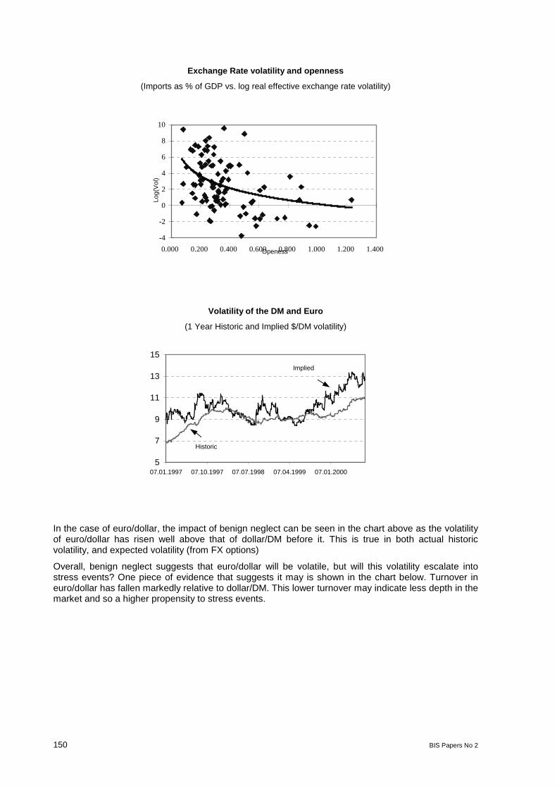
150 BIS Papers No 2
Exchange Rate volatility and openness
(Imports as % of GDP vs. log real effective exchange rate volatility)
-4
-2
0
2
4
6
8
10
0.000 0.200 0.400 0.600 0.800 1.000 1.200 1.400Openess
Log(
Vol
)
Volatility of the DM and Euro
(1 Year Historic and Implied $/DM volatility)
5
7
9
11
13
15
07.01.1997 07.10.1997 07.07.1998 07.04.1999 07.01.2000
Historic
Implied
In the case of euro/dollar, the impact of benign neglect can be seen in the chart above as the volatilityof euro/dollar has risen well above that of dollar/DM before it. This is true in both actual historicvolatility, and expected volatility (from FX options)
Overall, benign neglect suggests that euro/dollar will be volatile, but will this volatility escalate intostress events? One piece of evidence that suggests it may is shown in the chart below. Turnover ineuro/dollar has fallen markedly relative to dollar/DM. This lower turnover may indicate less depth in themarket and so a higher propensity to stress events.
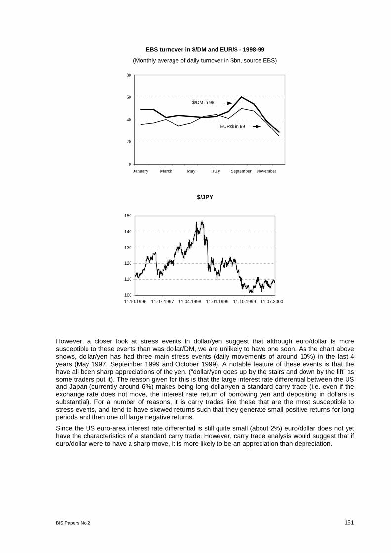
BIS Papers No 2 151
EBS turnover in $/DM and EUR/$ - 1998-99
(Monthly average of daily turnover in $bn, source EBS)
0
20
40
60
80
January March May July September November
$/DM in 98
EUR/$ in 99
$/JPY
100
110
120
130
140
150
11.10.1996 11.07.1997 11.04.1998 11.01.1999 11.10.1999 11.07.2000
However, a closer look at stress events in dollar/yen suggest that although euro/dollar is moresusceptible to these events than was dollar/DM, we are unlikely to have one soon. As the chart aboveshows, dollar/yen has had three main stress events (daily movements of around 10%) in the last 4years (May 1997, September 1999 and October 1999). A notable feature of these events is that thehave all been sharp appreciations of the yen. (“dollar/yen goes up by the stairs and down by the lift” assome traders put it). The reason given for this is that the large interest rate differential between the USand Japan (currently around 6%) makes being long dollar/yen a standard carry trade (i.e. even if theexchange rate does not move, the interest rate return of borrowing yen and depositing in dollars issubstantial). For a number of reasons, it is carry trades like these that are the most susceptible tostress events, and tend to have skewed returns such that they generate small positive returns for longperiods and then one off large negative returns.
Since the US euro-area interest rate differential is still quite small (about 2%) euro/dollar does not yethave the characteristics of a standard carry trade. However, carry trade analysis would suggest that ifeuro/dollar were to have a sharp move, it is more likely to be an appreciation than depreciation.
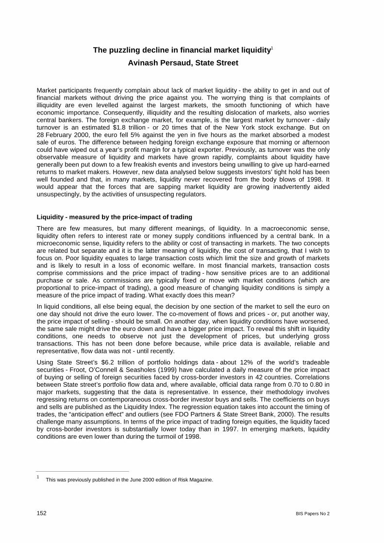
152 BIS Papers No 2
The puzzling decline in financial market liquidity1
Avinash Persaud, State Street
Market participants frequently complain about lack of market liquidity - the ability to get in and out offinancial markets without driving the price against you. The worrying thing is that complaints ofilliquidity are even levelled against the largest markets, the smooth functioning of which haveeconomic importance. Consequently, illiquidity and the resulting dislocation of markets, also worriescentral bankers. The foreign exchange market, for example, is the largest market by turnover - dailyturnover is an estimated $1.8 trillion - or 20 times that of the New York stock exchange. But on28 February 2000, the euro fell 5% against the yen in five hours as the market absorbed a modestsale of euros. The difference between hedging foreign exchange exposure that morning or afternooncould have wiped out a year’s profit margin for a typical exporter. Previously, as turnover was the onlyobservable measure of liquidity and markets have grown rapidly, complaints about liquidity havegenerally been put down to a few freakish events and investors being unwilling to give up hard-earnedreturns to market makers. However, new data analysed below suggests investors’ tight hold has beenwell founded and that, in many markets, liquidity never recovered from the body blows of 1998. Itwould appear that the forces that are sapping market liquidity are growing inadvertently aidedunsuspectingly, by the activities of unsuspecting regulators.
Liquidity - measured by the price-impact of trading
There are few measures, but many different meanings, of liquidity. In a macroeconomic sense,liquidity often refers to interest rate or money supply conditions influenced by a central bank. In amicroeconomic sense, liquidity refers to the ability or cost of transacting in markets. The two conceptsare related but separate and it is the latter meaning of liquidity, the cost of transacting, that I wish tofocus on. Poor liquidity equates to large transaction costs which limit the size and growth of marketsand is likely to result in a loss of economic welfare. In most financial markets, transaction costscomprise commissions and the price impact of trading - how sensitive prices are to an additionalpurchase or sale. As commissions are typically fixed or move with market conditions (which areproportional to price-impact of trading), a good measure of changing liquidity conditions is simply ameasure of the price impact of trading. What exactly does this mean?
In liquid conditions, all else being equal, the decision by one section of the market to sell the euro onone day should not drive the euro lower. The co-movement of flows and prices - or, put another way,the price impact of selling - should be small. On another day, when liquidity conditions have worsened,the same sale might drive the euro down and have a bigger price impact. To reveal this shift in liquidityconditions, one needs to observe not just the development of prices, but underlying grosstransactions. This has not been done before because, while price data is available, reliable andrepresentative, flow data was not - until recently.
Using State Street’s $6.2 trillion of portfolio holdings data - about 12% of the world’s tradeablesecurities - Froot, O’Connell & Seasholes (1999) have calculated a daily measure of the price impactof buying or selling of foreign securities faced by cross-border investors in 42 countries. Correlationsbetween State street’s portfolio flow data and, where available, official data range from 0.70 to 0.80 inmajor markets, suggesting that the data is representative. In essence, their methodology involvesregressing returns on contemporaneous cross-border investor buys and sells. The coefficients on buysand sells are published as the Liquidity Index. The regression equation takes into account the timing oftrades, the “anticipation effect” and outliers (see FDO Partners & State Street Bank, 2000). The resultschallenge many assumptions. In terms of the price impact of trading foreign equities, the liquidity facedby cross-border investors is substantially lower today than in 1997. In emerging markets, liquidityconditions are even lower than during the turmoil of 1998.
1This was previously published in the June 2000 edition of Risk Magazine.
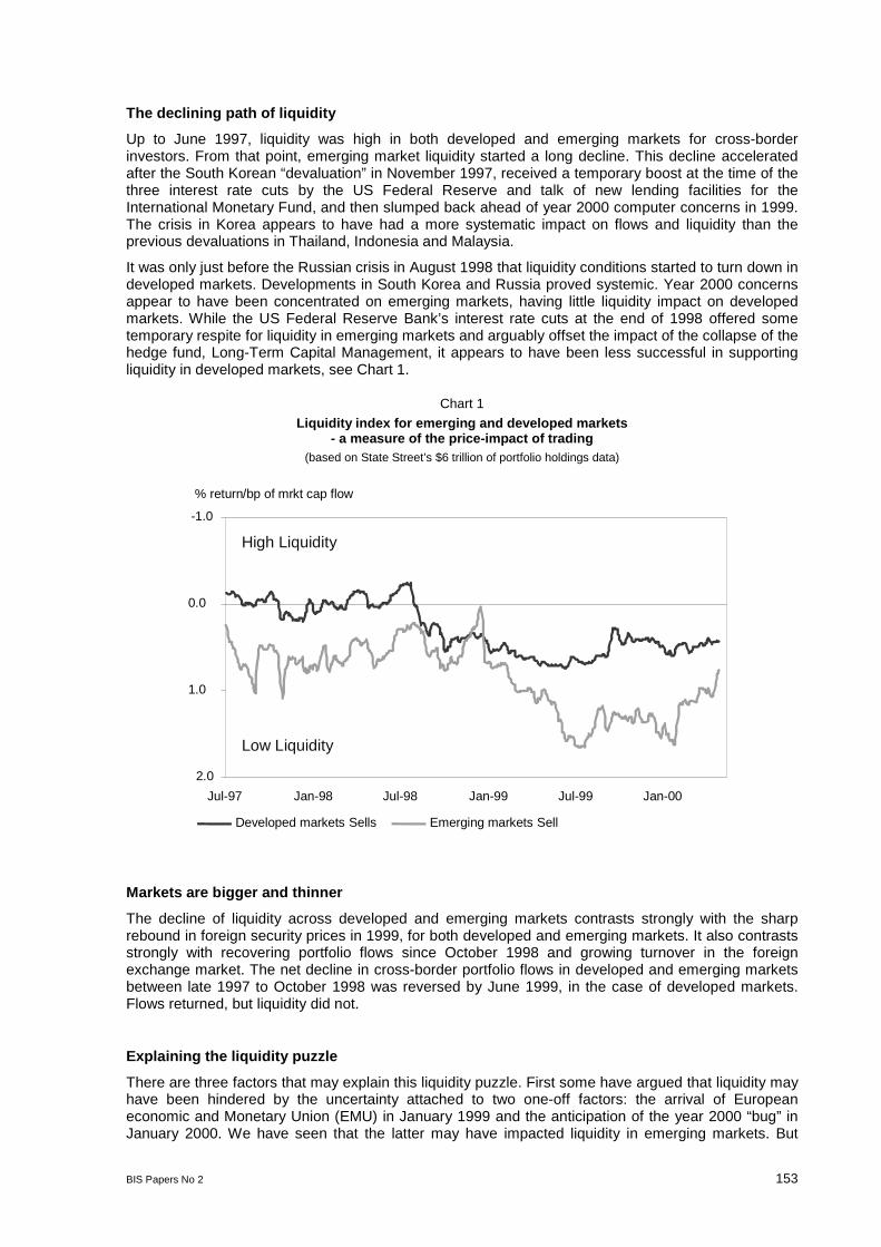
BIS Papers No 2 153
The declining path of liquidity
Up to June 1997, liquidity was high in both developed and emerging markets for cross-borderinvestors. From that point, emerging market liquidity started a long decline. This decline acceleratedafter the South Korean “devaluation” in November 1997, received a temporary boost at the time of thethree interest rate cuts by the US Federal Reserve and talk of new lending facilities for theInternational Monetary Fund, and then slumped back ahead of year 2000 computer concerns in 1999.The crisis in Korea appears to have had a more systematic impact on flows and liquidity than theprevious devaluations in Thailand, Indonesia and Malaysia.
It was only just before the Russian crisis in August 1998 that liquidity conditions started to turn down indeveloped markets. Developments in South Korea and Russia proved systemic. Year 2000 concernsappear to have been concentrated on emerging markets, having little liquidity impact on developedmarkets. While the US Federal Reserve Bank’s interest rate cuts at the end of 1998 offered sometemporary respite for liquidity in emerging markets and arguably offset the impact of the collapse of thehedge fund, Long-Term Capital Management, it appears to have been less successful in supportingliquidity in developed markets, see Chart 1.
Chart 1
Liquidity index for emerging and developed markets- a measure of the price-impact of trading
(based on State Street’s $6 trillion of portfolio holdings data)
-1.0
0.0
1.0
2.0
Jul-97 Jan-98 Jul-98 Jan-99 Jul-99 Jan-00
Developed markets Sells Emerging markets Sell
% return/bp of mrkt cap flow
High Liquidity
Low Liquidity
Markets are bigger and thinner
The decline of liquidity across developed and emerging markets contrasts strongly with the sharprebound in foreign security prices in 1999, for both developed and emerging markets. It also contrastsstrongly with recovering portfolio flows since October 1998 and growing turnover in the foreignexchange market. The net decline in cross-border portfolio flows in developed and emerging marketsbetween late 1997 to October 1998 was reversed by June 1999, in the case of developed markets.Flows returned, but liquidity did not.
Explaining the liquidity puzzle
There are three factors that may explain this liquidity puzzle. First some have argued that liquidity mayhave been hindered by the uncertainty attached to two one-off factors: the arrival of Europeaneconomic and Monetary Union (EMU) in January 1999 and the anticipation of the year 2000 “bug” inJanuary 2000. We have seen that the latter may have impacted liquidity in emerging markets. But
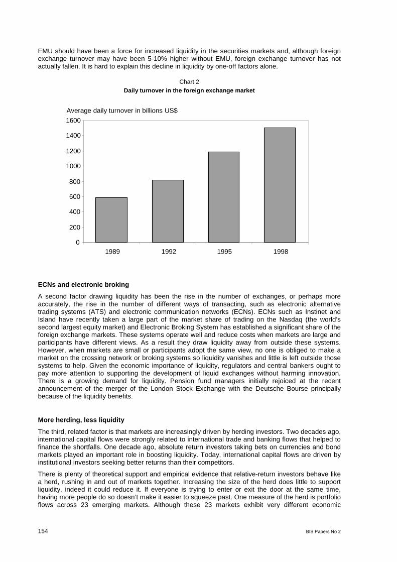
154 BIS Papers No 2
EMU should have been a force for increased liquidity in the securities markets and, although foreignexchange turnover may have been 5-10% higher without EMU, foreign exchange turnover has notactually fallen. It is hard to explain this decline in liquidity by one-off factors alone.
Chart 2
Daily turnover in the foreign exchange market
0
200
400
600
800
1000
1200
1400
1600
1989 1992 1995 1998
Average daily turnover in billions US$
ECNs and electronic broking
A second factor drawing liquidity has been the rise in the number of exchanges, or perhaps moreaccurately, the rise in the number of different ways of transacting, such as electronic alternativetrading systems (ATS) and electronic communication networks (ECNs). ECNs such as Instinet andIsland have recently taken a large part of the market share of trading on the Nasdaq (the world’ssecond largest equity market) and Electronic Broking System has established a significant share of theforeign exchange markets. These systems operate well and reduce costs when markets are large andparticipants have different views. As a result they draw liquidity away from outside these systems.However, when markets are small or participants adopt the same view, no one is obliged to make amarket on the crossing network or broking systems so liquidity vanishes and little is left outside thosesystems to help. Given the economic importance of liquidity, regulators and central bankers ought topay more attention to supporting the development of liquid exchanges without harming innovation.There is a growing demand for liquidity. Pension fund managers initially rejoiced at the recentannouncement of the merger of the London Stock Exchange with the Deutsche Bourse principallybecause of the liquidity benefits.
More herding, less liquidity
The third, related factor is that markets are increasingly driven by herding investors. Two decades ago,international capital flows were strongly related to international trade and banking flows that helped tofinance the shortfalls. One decade ago, absolute return investors taking bets on currencies and bondmarkets played an important role in boosting liquidity. Today, international capital flows are driven byinstitutional investors seeking better returns than their competitors.
There is plenty of theoretical support and empirical evidence that relative-return investors behave likea herd, rushing in and out of markets together. Increasing the size of the herd does little to supportliquidity, indeed it could reduce it. If everyone is trying to enter or exit the door at the same time,having more people do so doesn’t make it easier to squeeze past. One measure of the herd is portfolioflows across 23 emerging markets. Although these 23 markets exhibit very different economic
BIS Papers No 2 155
fundamentals, politics and markets, there are times when all 23 markets are receiving net inflows as inmost of 1996 when buying emerging markets was all the rage, or in late 1998, when almost all 23were receiving net outflows. Chart 3 shows the ratio of the number of emerging market countriesreceiving net cross-border inflows over the previous month (or more precisely, rolling 20 businessdays). This ratio can be used as a measure of investors’ preference or aversion to risk more generally.
Chart 3
Ratio of emerging markets receiving net cross-border inflows(based on State Street’s $6 trillion portfolio holdings data)
0.0
0.5
1.0
Jan-96 Jan-97 Jan-98 Jan-99 Jan-00
Ratio
Risk management may make matters worse
To some extent, the combination of herding investors and tighter risk management systems hasaggravated liquidity conditions. Herding investors hit their risk management limits together, causingthem to sell the same markets together, reducing liquidity and causing those markets to exhibit evengreater volatility than in the past, which in turn feeds back into risk management systems and leads tofurther sales. Thus, the cycle becomes self-feeding. In these environments, markets need contrarianinvestors able to run sizeable losses and buy near the bottom in the hope that they will be the first tobenefit from the turnaround. Interestingly, unregulated, hedge funds are more likely to do this thanregulated investors and banks. Indeed, given that such hedge funds are putting the risk capital ofwealthy professionals at risk (and not the life savings of the average person in the street), they areeminently suitable for this task.
Hedge funds may support liquidity
The irony is that, by pressuring counterparties to insist on greater disclosure and tougher collateralrequirements, regulators have been discouraging the kind of hedge funds that make big macro bets. Inthe process, they may have damaged market liquidity which in turn has made it more difficult for thesehedge funds to operate. It is noteworthy that the pattern of liquidity faced by cross-border institutionalinvestors in emerging markets follows very closely the dwindling size of macro hedge funds. Thisprocess has recently enveloped the twin icons of the hedge fund industry, Julian Robertson andGeorge Soros.
Regulators need to examine how to achieve the right balance of regulation and provide support toliquidity. Given that herding by institutional investors continues, that ECNs and ATSs are growing innumber and that big macro hedge funds are on the defensive, one can expect liquidity to remain in
156 BIS Papers No 2
scarce supply. Consequently, the managing of liquidity will become increasingly important for everyparticipant in financial markets. With this in mind, and armed with this new set of daily data on liquidityin 41 different markets (Froot, O’Connell & Seasholes, 1999), State Street intend to initiate a regularseries of research on liquidity, its path, its drivers and key changes.
Avinash Persaud, Global Head of Research
Summary of methodology
The Liquidity Index (see main text) was produced by FDO partners, LLC and State Street Bank. StateStreet Bank is the world’s largest custodian with more than $6.2 trillion of assets under custody. TheLiquidity Index is based on daily cross-border transactions data, collected by State Street Bank &Trust. From the universe of total daily transactions, State Street separates out only those transactionsthat originate in one country but settle in another currency - cross-border portfolio flows.
The methodology involves regressing returns on contemporaneous buys and sells. The coefficients onbuys and sells from the regression are published as the “Liquidity Index - a measure of the priceimpact of trading”. The regression specification takes into account the timing of trades, the“anticipation effect” and outliers.
This measure is both a measure of liquidity faced by cross-border investors and a measure of whethercross-border flows are “driving” the current direction of a market or not. Either interpretation can bejustified.
Adjustment to the data
Timing of trades, anticipation effects, outliers
In order to take into account the fact that a trade can take place in the same day but across severaltime zones, each day’s data is actually the average of returns on that day and the preceding day.
Earlier work by Professor Ken Froot et al has shown that State Street’s portfolio flows have predictivepower for future equity returns. To try to isolate the contemporaneous price impact of trades, thiscorrelation is controlled for by including lagged terms of buys and sells in the regression specification.
A single outlier can cause coefficients to shift wildly, as the outlier enters the rolling window used toestimate the regression and when it leaves. In order to reduce these distortions outliers are removedin the following way. Each day, for each country, the amount of bought and sold (as a fraction ofmarket capitalisation) is compared to the mean buy or sell trades over the past trading days. Any pointthat is more than four standard deviations away from the mean is replaced with the mean.
Regression equation
To estimate the price impact cost, we run a regression of returns on contemporaneous buys,contemporaneous sells, lagged buys, lagged sells and a constant.
Ri,t = i + θB,i Buyi,t + θS,i Selli,t + B,i Buyi,t–p + S,i Selli,t–p + εi,t
where:
Ri,t = the average daily return of market “i” over the week from “t–(p+1)” to “t”
Buyi,t = the average fraction of market capitalization of market “i” bought by clients of State StreetBank over the week from “t–(p+1)” to “t”
Selli,t = the average fraction of market capitalization of market “i” sold by clients of State Street Bankover the week from “t–(p+1)” to “t”
The two parameters of interest are:
θB,i parameter related to the price impact of foreign buying
θS,i parameter related to the price impact of foreign selling

BIS Papers No 2 157
We expect the parameter θB,i to be positive most of the time, indicating that foreign purchases happencontemporaneously with price increases. During periods when the price impact costs of buying arehigh, the θB,i parameter will be more positive than during times when the price impact costs are low.
Likewise, we expect the θS,i parameter to be negative, indicating that foreign sales happencontemporaneously with price decreases. During periods when the price impact costs of selling arehigh, the θS,i parameter will be more negative than during times when the price impact costs are low.Here because the θS,i parameter is multiplied by –1, it will be reflected into the positive y-axis.
The magnitude of the parameters depends on a number of factors including State Street’s share offoreign trading in a particular market and the units that the flows and returns are recorded in(eg decimal form, percentages, basis points, etc). We express returns (in USD) in percentages(multiply them by 100) and flows in basis points of market capitalization (multiply them by 10,000).
Contemporaneous correlation
Returns are highly correlated in markets around the world. To account for this correlation, we estimatea system of regression equations and allow for correlation between the residuals. For one region orcountry, we have:
Ri,t = i + θB,i Buyi,t + θS,i Selli,t + B,i Buyi,t–p + S,i Selli,t–p + εi,t
which can be written more succinctly: Yi = Xi i + εi
We then stack a series of regions or countries:
+
=
NNN X
X
X
Y
Y
Y
ε
εε
β
ββ
2
1
2
1
1
1
1
2
1
00
00
00
=Σ
NNNN
N
N
σσσ
σσσσσσ
21
22221
11211
The GLS estimator is:
[ ] YVXXVX
IV N
111 ’’ˆ −−−=
⊗Σ=
β
The GLS estimator β is actually a vector of region or country parameters [ ] /21
ˆ,,ˆ,ˆˆNββββ = where
each region or country parameter is [ ]/
,,,,ˆ,ˆ,ˆ,ˆ,ˆˆ
iSiBiSiBi ΛΛ= θθαβ . Again, we are interested only in the
parameter estimates of iSiB ,,ˆ,ˆ θθ which represent the contemporaneous co-movement of prices and
flows.
All regions and countries are unable to be estimated together because regions are linear combinationsof countries
For further detail see, Liquidity Index - Technical Document, FDO Partners LLC & State Street Bank,April 2000.

158 BIS Papers No 2
References
Brennan, Michael J and H Henry Cao (1997): “International Portfolio Investment Flows”, Journal ofFinance, 52, December, 1851-1880.
Choe, Hyuk, Bond-Chan Kho and Rene Stulz (1998): “Do Foreign Investors Destabilize StockMarkets? The Korean Experience in 1997”, working paper manuscript, October.
De Long, J Bradford, Andrei Shleifer, Lawrence H Summers and Robert J Waldmann (1990): “NoiseTrader Risk in Financial Markets”, Journal of Political Economy, 98, No 4, 703-738.
Frankel, Jeffrey A and Sergio L Schmukler (1998): “Country Funds and Asymmetric Information”,Policy Research Working Paper No 1886, World Bank, Washington DC.
Froot, Kenneth A, Paul G J O’Connell and Mark S Seasholes (1999): “The Portfolio Flows ofInternational Investors, I”, Harvard Business School Working Paper.
International Finance Corporation (1999): IFC Emerging Stock Market Factbook, International FinanceCorporation, Washington DC.
Kim, Woochan and Shang-Jin Wei (1999a): “Foreign Portfolio Investors Before and During a Crisis”,Working Paper, Harvard University.
Kyle, Albert S (1985): “Continuous Auctions and Insider Trading”, Econometrica, 53, 1315-1336.
Wermers, Russ (1998): “Mutual Fund Herding and the Impact on Stock Prices”, Journal ofFinance, 54, No 2, 581-622.

BIS Papers No 2 159
Measuring liquidity under stress
Christian Upper, Deutsche Bundesbank
In my contribution to the panel, I want to focus on how to measure liquidity under stress. Sincefinancial markets seem to behave quite differently in periods of stress than under normal conditions,measures of liquidity that tend to work well most of the time may no longer be meaningful in turbulentmarkets.
In line with much of the literature, I define market liquidity as the “ease” with which a security can betraded. The word “ease” can be substituted by the word “cost”. The cost of trading includescommissions, fees and taxes as well as the bid-ask spread, the price impact of a trade, and the costcaused by prices movements if a trade cannot be executed at once or when it is split up into asequence of smaller transactions. In normal times, the cost of trading is particular relevant for thoseinvestors who try to make a profit by trading on small movements in prices and, consequently, turnover positions relatively quickly. For such agents, even small differences in the cost of a transactioncan make or break a trading strategy. Investors with longer time horizons shouldn’t really worry aboutmarket liquidity.
In periods of stress, the relative importance of the individual factors determining market liquiditychanges. Prices become much more volatile than they are normally, and a strong desire on part of thetraders to close undesired positions seems to dominate all other motivations for trading. Fromconversations with practitioners, I have the impression that costs arising from the price impact oftrades or the inability to close positions quickly when prices are moving against them tend to eclipsethe bid-ask spread and administrative costs. As a consequence, any measure for liquidity under stressshould meet two requirements:
1. it should reflect the costs of closing large positions quickly; and
2. it should be available at a relatively high frequency as even relatively brief bouts of illiquiditymay impose heavy costs on market participants if prices are volatile.
In order to illustrate the issues involved, I consider the liquidity of 10 year German government bondsmarket during two episodes of stress. The first took place in the aftermath of the Russian debtmoratorium on 17 August, and the second during the sharp revaluation of the yen vis-à-vis the USdollar on 8 and 9 October of the same year.1 As you will find out, the microstructure of the Germanbond market is broadly similar to that of foreign exchange markets, so the discussion should havesome relevance beyond the particular market segment considered.
Although German government bonds are listed, the role of exchanges is negligible, with the bulk oftrading taking place over the counter. This is especially true for the inter-dealer market, where tradingtakes place either directly between banks or through inter-dealer brokers (Freimakler). These act asintermediaries, but have no obligation to provide firm quotes. More recently, a sizeable proportion ofinter-dealer trading has shifted to the electronic trading systems Euro-MTS, but electronig trading didnot exist in 1998. The OTC market seems to be altogether rather opaque. Participants observe quotesbut do not receive timely information on other traders’ past transactions beyond anecdotal evidence.The only comprehensive data set is maintained by the German securities regulator, which receivesinformation on every single transaction in Germany, regardless of whether or not it takes place on anexchange. However, this data is not published on a regular basis - not even in aggregated form -although it has been available for research purposes.
After this brief excursion into the microstructure of the German government bond market, let me turn toour main topic. A measure for liquidity that is often used by practitioners is trading volume. As amacroeconomist raised on representative agent models, where markets can be liquid without anytrades actually taking place, I initially found this surprising. Market liquidity is only one, and notnecessarily the most important, factor affecting trading activity. For example, if traders have sufficientlylarge hedging needs, then they may trade even if market liquidity is relatively low. What volume doestell us, however, is whether trading was possible at all.
1The analysis is based on Upper (2000).

160 BIS Papers No 2
Turnover in the German government bond market was particularly high just after the Russian debtmoratorium, with a high average size of trade. Both turnover and the average trade size declinedthroughout September, and remained relatively - but not unusually - low on 8 and 9 October. Shouldwe conclude that the market was very liquid during the first episode but not during the second? Notnecessarily. Perhaps market participants had much stronger hedging needs after the Russianmoratorium than during the events in the forex market.
A measure for liquidity that is easily available at any frequency and is directly linked to the cost oftrading is the quoted bid-ask spread. However, since there is no commitment to market making in theOTC market for Bundesanleihen, quoted spreads are merely indicative, ie agents do not have tohonour the prices they promise. While this should not matter in normal times, it is a problem in periodsof stress. Traders told me that in the aftermath of the Russian moratorium, some traders simply did notbother to answer the phone. In addition, quoted spreads apply to transactions up to a specifiedamount only, which, furthermore, may vary over time. Eg if market participants cut this amount inperiods of stress, then this would leave the quoted spread unchanged, even though market depthwould fall.
One way out is to compute effective spreads from transactions data.2 Unlike quoted spreads, effectivespreads refer to the average transaction and therefore capture at least some of the cost of closinglarge positions. Unfortunately, this comes at a cost. Effective spreads have to be estimated, whichintroduces noise and reduces the frequency at which they are available. For the four Germangovernment bonds of our sample, the highest frequency which could be computed was one day.
Figure 2 shows the effective bid-ask spreads computed with Roll’s (1984) measure. While thismeasure has important shortcomings3, it is easy to estimate and does require a direction of tradeindicator (which I have not been able to construct). I find that effective bid-ask spreads rose fromvalues of less than one basis point during the first, tranquil, half of the year to 2-2½ basis points duringthe second half of August. This clearly indicates a reduction in market liquidity, in contrast to theincrease suggested by the turnover series. Effective spreads gradually declined until the beginning ofOctober, but soared to to around 4 basis points on 8 and 9 October.
How can we interpret the apparently contradictory findings of the activity series and the bid-askspreads? First of all, the two measures should be viewed in conjunction. The increase in spreads afterthe Russian moratorium looks less menacing if we bear in mind that the market has been able tohandle a considerably higher volume as well as larger trade sizes than under normal conditions. Inearly October, in contrast, there was no surge in volume which could explain at least part of thewidening of the bid-ask spreads, which therefore looks much more threatening.
Let me conclude by restating the two requirements that a measure for liquidity under stress shouldmeet. Firstly, it should reflect the cost of closing large positions within a short period of time. Secondly,it should be available at high frequencies. Neither trading volume nor the effective bid-ask spreadconsidered completely satisfy both requirements on their own. Taken together, however, we do get afair picture of a market that seems to have been rather effective in handling a high degree of activity inAugust but became rather illiquid in October.
The ascent of electronic trading should - in principle - open up new sources of high quality data, whichwould permit us to compute more elaborate measures of liquidity. It is crucial, though, that centralbanks actually get access to this data. The experience in this respect has so far not been veryencouraging.
2For a survey of different ways to compute effective spreads refer to Huang & Stoll (1997).
3In particular, the Roll-measure is biased downwards in the presence of asymmetric information or inventory effects. Sincesuch effects are more likely to occur in times of stress when price volatility adds to inventory risk and there may be morescope for private information, the Roll measure probably underestimates any stress-related reduction of market liquidity.

BIS Papers No 2 161
References
Huang, R D & H R Stoll (1997) “The Components of the Bid-Ask Spread: A General Approach”,Review of Financial Studies, 10(4):
Roll, R (1984) “A Simple Implicit Measure of the Effective Bid-Ask Spread in an Efficient Market”,Journal of Finance, 39: 1127-40
Upper, C (2000) “How Safe was the ‘Safe Haven’? Financial Market Liquidity during the 1998Turbulences”, Economic Research Group of the Deutsche Bundesbank, Discussion Paper 1/00.
BIS Papers No 2 165
Order flow and exchange rate dynamics
Martin D D Evans1 and Richard K Lyons
Abstract
Macroeconomic models of nominal exchange rates perform poorly. In sample, R2 statistics as high as10% are rare. Out of sample, these models are typically out-forecast by a naïve random walk. Thispaper presents a model of a new kind. Instead of relying exclusively on macroeconomic determinants,the model includes a determinant from the field of microstructure- order flow. Order flow is theproximate determinant of price in all microstructure models. This is a radically different approach toexchange rate determination. It is also strikingly successful in accounting for realised rates. Our modelof daily changes in log exchange rates produces R2 statistics above 50%. Out of sample, our modelproduces significantly better short-horizon forecasts than a random walk. For the DM/$ spot market asa whole, we find that $1 billion of net dollar purchases increases the DM price of a dollar by about0.5%.
Omitted variables is another possible explanation for the lack of explanatory powerin asset market models. However, empirical researchers have shown considerableimagination in their specification searches, so it is not easy to think of variables thathave escaped consideration in an exchange rate equation.
Richard Meese (1990)
1. Motivation: microstructure meets exchange rate economics
Since the landmark papers of Meese and Rogoff (1983a, 1983b), exchange rate economics has beenin crisis. It is in crisis in the sense that current macroeconomic approaches to exchange rates areempirical failures: the proportion of monthly exchange rate changes that current models can explain isessentially zero. In their survey, Frankel and Rose (1995) write “the Meese and Rogoff analysis atshort horizons has never been convincingly overturned or explained. It continues to exert a pessimisticeffect on the field of empirical exchange rate modelling in particular and international finance ingeneral.”2
Which direction to turn is not obvious. Flood and Rose (1995), for example, are “driven to theconclusion that the most critical determinants of exchange rate volatility are not macroeconomic.” Ifdeterminants are not macro fundamentals like interest rates, money supplies, and trade balances,then what are they? Two alternatives have attracted attention. The first is that exchange ratedeterminants include extraneous variables. These extraneous variables are typically modeled asrational speculative bubbles (Blanchard 1979, Dornbusch 1982, Meese 1986, and Evans 1986, amongothers). Though the jury is still out, Flood and Hodrick (1990) conclude that the bubble alternativeremains unconvincing. A second alternative to macro fundamentals is irrationality. For example,exchange rates may be determined in part from avoidable expectational errors (Dominguez 1986,Frankel and Froot 1987, and Hau 1998, among others). On a priori grounds, many economists findthis second alternative unappealing. Even if one is sympathetic to the presence of irrationality, there isa wide gulf between its presence and accounting for exchange rates empirically. Until it can producean empirical account, this too will remain an unconvincing alternative.
1 Respective affiliations are Georgetown University and NBER, and UC Berkeley and NBER. We thank the following for
valuable comments: two anonymous referees, Menzie Chinn, Peter DeMarzo, Frank Diebold, Petra Geraats, Eric Jondeau,Robert McCauley, Richard Meese, Michael Melvin, Peter Reiss, Andrew Rose, Mark Taranto, Ingrid Werner, Alwyn Young,and seminar participants at Chicago, Wharton, Columbia, MIT, Iowa, Houston, Stanford, UC Berkeley, the 1999 NBERSummer Institute (IFM), the December 1999 NBER program meeting in Microstructure, and the August 2000 BIS workshopon Market Liquidity. Lyons thanks the National Science Foundation for financial assistance.
2 The relevant literature is vast. Recent surveys include Frankel and Rose (1995), Isard (1995), and Taylor (1995).
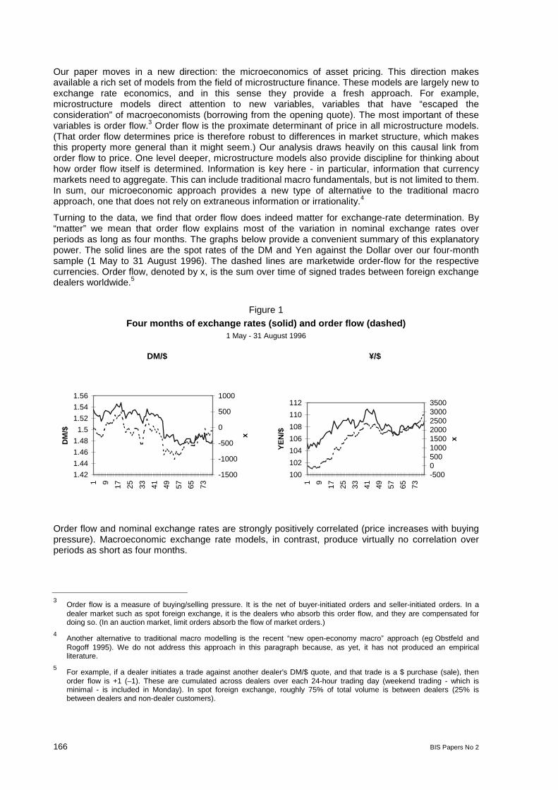
166 BIS Papers No 2
Our paper moves in a new direction: the microeconomics of asset pricing. This direction makesavailable a rich set of models from the field of microstructure finance. These models are largely new toexchange rate economics, and in this sense they provide a fresh approach. For example,microstructure models direct attention to new variables, variables that have “escaped theconsideration” of macroeconomists (borrowing from the opening quote). The most important of thesevariables is order flow.3 Order flow is the proximate determinant of price in all microstructure models.(That order flow determines price is therefore robust to differences in market structure, which makesthis property more general than it might seem.) Our analysis draws heavily on this causal link fromorder flow to price. One level deeper, microstructure models also provide discipline for thinking abouthow order flow itself is determined. Information is key here - in particular, information that currencymarkets need to aggregate. This can include traditional macro fundamentals, but is not limited to them.In sum, our microeconomic approach provides a new type of alternative to the traditional macroapproach, one that does not rely on extraneous information or irrationality.4
Turning to the data, we find that order flow does indeed matter for exchange-rate determination. By“matter” we mean that order flow explains most of the variation in nominal exchange rates overperiods as long as four months. The graphs below provide a convenient summary of this explanatorypower. The solid lines are the spot rates of the DM and Yen against the Dollar over our four-monthsample (1 May to 31 August 1996). The dashed lines are marketwide order-flow for the respectivecurrencies. Order flow, denoted by x, is the sum over time of signed trades between foreign exchangedealers worldwide.5
Figure 1
Four months of exchange rates (solid) and order flow (dashed)1 May - 31 August 1996
DM/$ ¥/$
Order flow and nominal exchange rates are strongly positively correlated (price increases with buyingpressure). Macroeconomic exchange rate models, in contrast, produce virtually no correlation overperiods as short as four months.
3Order flow is a measure of buying/selling pressure. It is the net of buyer-initiated orders and seller-initiated orders. In adealer market such as spot foreign exchange, it is the dealers who absorb this order flow, and they are compensated fordoing so. (In an auction market, limit orders absorb the flow of market orders.)
4Another alternative to traditional macro modelling is the recent “new open-economy macro” approach (eg Obstfeld andRogoff 1995). We do not address this approach in this paragraph because, as yet, it has not produced an empiricalliterature.
5For example, if a dealer initiates a trade against another dealer's DM/$ quote, and that trade is a $ purchase (sale), thenorder flow is +1 (–1). These are cumulated across dealers over each 24-hour trading day (weekend trading - which isminimal - is included in Monday). In spot foreign exchange, roughly 75% of total volume is between dealers (25% isbetween dealers and non-dealer customers).
1.42
1.44
1.46
1.48
1.5
1.52
1.54
1.56
1 9 17 25 33 41 49 57 65 73
DM
/$
-1500
-1000
-500
0
500
1000
x
100
102
104
106
108
110
112
1 9 17 25 33 41 49 57 65 73
YE
N/$
-5000500100015002000250030003500
x
BIS Papers No 2 167
To address this more formally, we develop and estimate a model that includes both macroeconomicdeterminants (eg interest rates) and a microstructure determinant (order flow). Our estimates verify thesignificance of the above correlation. The model accounts for about 60% of daily changes in the DM/$exchange rate. For comparison, macro models rarely account for even 10% of monthly changes. Ourdaily frequency is noteworthy: though our model draws from microstructure, it is not estimated at thetransaction frequency. Daily analysis is in the missing middle between past microstructure work (tick-by-tick data) and past macro work (monthly data). Bridging the two helps clarify how lower-frequencyexchange rates emerge from the market’s operation in real time.
To complement these in-sample results, we also examine the model’s out-of-sample forecastingability. Work by Meese and Rogoff (1983a) examines short-horizon forecasts (1 to 12 months). Theyfind that a random walk model out-forecasts the leading macro models, even when macro-model“forecasts” are based on realised future fundamentals. Subsequent work lengthens the horizonbeyond 12 months and finds that macro models begin to dominate the random walk (Meese andRogoff 1983b, Chinn 1991, Chinn and Meese 1994, and Mark 1995). But results at shorter horizonsremain a puzzle. Here we examine horizons of less than one month. (Transaction data sets that arecurrently available are too short to generate statistical power at monthly horizons.) We find that athorizons from one-day to two-weeks, our model produces better forecasts than the random-walkmodel (over 30% lower root mean squared error).
The relation we find between exchange rates and order flow is not inconsistent with the macroapproach, but it does raise several concerns. Under the macro approach, order flow should not matterfor exchange rate determination: macroeconomic information is publicly available - it is impounded inexchange rates without the need for order flow. More precisely, the macro approach typically assumesthat: (1) all information relevant for exchange rate determination is common knowledge; and (2) themapping from that information to equilibrium prices is also common knowledge. If either of these twoassumptions is relaxed, however, then order flow will convey information about market-clearing prices.Relaxing the second assumption should not be controversial, given the failure of currentexchange-rate models. Direct evidence, too, corroborates that order flow conveys relevant information(Lyons 1995, Yao 1997, Covrig and Melvin 1998, Ito, Lyons and Melvin 1998, Cheung and Wong1998, Bjonnes and Rime 1998, Evans 1999, Naranjo and Nimalendran 1999, and Payne 1999.)6
Note that order flow being a proximate determinant of exchange rates does not preclude macrofundamentals from being the underlying determinant. Macro fundamentals in exchange rate equationsmay be so imprecisely measured that order-flow provides a better “proxy” of their variation. Thisinterpretation of order flow as a proxy for macro fundamentals is particularly plausible with respect toexpectations: standard empirical measures of expected future fundamentals are obviously imprecise.7
Orders, on the other hand, reflect a willingness to back one’s beliefs with real money (unlikesurvey-based measures of expectations). Measuring order flow under this interpretation is akin tocounting the backed-by-money expectational votes.
This paper has six remaining sections. Section two contrasts the micro and macro approaches toexchange rates. Section three develops a model that includes both micro and macro determinants.Section four describes our data. Section five presents our results. Section six provides perspective onour results. Section seven concludes.
6The standard example of order flow that conveys non-public information is orders from central bank intervention. (Within ourfour-month sample, however, the Fed never intervened.) Probably more important on an ongoing basis is order flow thatconveys information about “portfolio shifts” that are not common knowledge. A recent event provides a sharp example.Major banks attribute the yen/dollar rate’s drop from 145 to 115 in Fall 1998 to “the unwinding of positions by hedge fundsthat had borrowed in cheap yen to finance purchases of higher-yielding dollar assets” (The Economist, 10.10.98). Thisunwinding - and the selling of dollars that came with it - was forced by the scaling back of speculative leverage in themonths following the Long Term Capital Management crisis. These trades were not common knowledge as they wereoccurring. (See also section 6 below, and Cai et al. 1999.)
7One might argue that expectations measurement cannot be driving the negative results of Meese and Rogoff because theyuse the driving variables’ realised values. However, if the underlying macro model is incomplete, then realised values stillproduce an incorrect expectations measure.

168 BIS Papers No 2
2. Models: spanning the micro-macro divide
A core distinction between a microstructure approach to exchange rates and the traditional macroapproach is the role of trades in price determination. In macro models, trades have no distinct role indetermining price. In microstructure models, trades have a leading role - they are the proximate causeof price adjustment. It is instructive to frame this distinction by contrasting the structural models thatemerge from these two approaches.
Structural models: macro approach
Exchange-rate models within the macro approach are typically estimated at the monthly frequency.When estimated in changes they take the form:
(1) ∆pt = f(∆i, ∆m, …) + εt.
where ∆pt is the change in the log nominal exchange rate over the month (DM/$). The drivingvariables in the function f(∆i,∆m,…) include changes in home and foreign nominal interest rates i,money supply m, and other macro determinants, denoted here by the ellipsis.8 Changes in thesepublic-information variables drive price - there is no role for order flow. Any incidental price effectsfrom order flow that might arise are subsumed in the residual εt. These models are logically coherentand intuitively appealing. Unfortunately, they account for almost none of the monthly variation infloating exchange rates.
Structural models: microstructure approach
Equations of exchange-rate determination within the microstructure approach are derived from theoptimisation problem faced by price setters in the market - the dealers.9 These models are allvariations on the following specification:
(2) ∆pt = g(∆x, ∆I, …) + νt
Now ∆pt is the DM/$ rate change over two transactions, rather than over a month as in the macromodels. The driving variables in the function g(∆x,∆I,…) include order flow ∆x, the change in net dealerpositions (or inventory) ∆I, and other micro determinants, denoted by the ellipsis. Order flow can takeboth positive and negative values because the counterparty either purchases (+) at the dealer’s offeror sells at the dealer’s bid (–). Here we use the convention that a positive ∆x is net dollar purchases,making the theoretical relation positive: net dollar purchases drive up the DM price of dollars. It isinteresting to note that the residual in this case is the mirror image of the residual in equation 1: itsubsumes any price changes due to determinants in the macro model f(∆i,∆m,…), whereas theresidual in equation 1 subsumes price changes due to determinants in the micro model g(∆x,∆I,…).
Microstructure models predict a positive relation between ∆p and ∆x because order flowcommunicates non-public information, and once communicated, it is reflected in price. For example, ifthere is an agent who has superior information about the value of an asset, and that informationadvantage induces the agent to trade, then a dealer can learn from those trades (purchases indicategood news about the asset’s value, and vice versa). Empirically, estimates of a relation between ∆pand ∆x at the transaction frequency are uniformly positive and significant. This is true for manydifferent markets, including stocks, bonds, and foreign exchange.
The relation in microstructure models between ∆p and ∆I is not our focus in this paper, but let us clarifynonetheless. This relation is referred to as the inventory-control effect on price. The inventory-controleffect arises when a dealer adjusts his price to control fluctuation in his inventory. For example, if a
8The precise list of determinants depends on the model. Meese and Rogoff (1983a) focus on three models in particular: theflexible-price monetary model, the sticky-price monetary model, and the sticky-price asset model. Here our interest is simplya broad-brush contrast between the macro and microstructure approaches. For specific models see Frenkel (1976),Dornbusch (1976), and Mussa (1976), among many others.
9 Empirical work using structural micro models includes Glosten and Harris (1988), Madhavan and Smidt (1991), and Foster
and Viswanathan (1993), all of which address the NYSE. Structural models in a multiple-dealer setting include Snell andTonks (1995) for stocks, Lyons (1995) for currencies, and Vitale (1998) for bonds.
BIS Papers No 2 169
dealer has a larger long position than is desired, he may shade his bid and offer downward to induce acustomer purchase, thereby reducing his position. This affects realised transaction prices, whichaccounts for the relation. (These idiosyncratic inventory effects on individual dealer prices do not arisein the model developed in the next section.)
Spanning the micro-macro divide
To span the divide between the micro and macro approaches, we develop a model with componentsfrom both:10
(3) ∆pt = f(∆i,…) + g(∆x,…) + ηt.
The challenge is the frequency mismatch: transaction frequency for the micro models versus monthlyfrequency for the macro models. In the next section we develop a model in the spirit of equation (3).We estimate the model at the daily frequency by using micro determinants that are time-aggregated.We focus in particular on order flow ∆x. Our time-aggregated measure spans a much longer periodthan is addressed elsewhere within empirical microstructure.
3. Portfolio shifts model
Overview
One source of exchange rate variation in the model is portfolio shifts on the part of the public. Theseportfolio shifts have two important features. First, they are not common knowledge as they occur.Second, they are large enough that clearing the market requires adjustment of the spot exchange rate.
The first feature - that portfolio shifts are not common knowledge - provides a role for order flow. At thebeginning of each day, public portfolio shifts are manifested in orders in the foreign exchange market.These orders are not publicly observable. Dealers take the other side of these orders, and then tradeamong themselves during the day to share the resulting inventory risk. The market learns about theinitial portfolio shifts by observing this interdealer trading activity. By the end of the day, the dealers’inventory risk is shared with the public.
The second important feature is that the initial portfolio shifts, once absorbed by the public at the endof the day, are large enough to move price. This requires that the public’s demand for foreign-currencyassets is less than perfectly elastic. If the public’s demand is less than perfectly elastic, different-currency assets are imperfect substitutes, and price adjustment is required to clear the market.11 Inthis sense, our model is in the spirit of the portfolio balance approach to exchange rates. In anothersense, however, our model is very different from that earlier approach. Portfolio balance models aredriven by changes in asset supply. Asset supply is constant in our model. Rather, our model identifiestwo distinct components on the demand side. The first is driven by innovations in public information(standard macro fundamentals). The second is driven by non-public information. This non-publicinformation takes the form of portfolio shifts. The model does not take a stand on the underlyingdeterminants of these portfolio shifts (though we do address this issue in section 6).
10Goldberg and Tenorio (1997) develop a model for the Russian ruble market that includes both macro and microstructurecomponents. Osler’s (1998) trading model includes macroeconomic “current account traders” who affect the exchange ratein flow equilibrium.
11For evidence of imperfect substitutability across U.S. stocks, see Scholes (1972), Shleifer (1986) and Bagwell (1992),among others. Substitutability across currencies is likely to be lower than across same-currency stocks. Though directevidence of this lower substitutability is lacking, some point to home bias in international portfolios as indirect evidence.Note, too, that the size of the order flows the DM/$ spot market needs to absorb are on average more than 10,000 timesthose absorbed in a representative U.S. stock (eg the average daily volume on NYSE stocks in 1998 was $9.3 million,whereas the average daily volume in DM/$ spot was about $300 billion).

170 BIS Papers No 2
Specifics
Consider a pure exchange economy with T trading periods and two assets, one riskless, and one witha stochastic payoff representing foreign exchange. The T+1 payoff on foreign exchange, denoted F, is
composed of a series of increments, so that F=∑ +
=
1T
1t tr . The increments rt are i.i.d. Normal(0,Σr) and
are observed before trading in each period. These realised increments represent the flow of publiclyavailable macroeconomic information over time (eg changes in interest rates).
The foreign exchange market is organised as a decentralised dealership market with N dealers,indexed by i, and a continuum of non-dealer customers (the public), indexed by z∈ [0,1]. Within eachperiod (day) there are three rounds of trading. In the first round dealers trade with the public. In thesecond round dealers trade among themselves to share the resulting inventory risk. In the third rounddealers trade again with the public to share inventory risk more broadly. The timing within each periodis:
Daily timing
Round 1 Round 2 Round 3
rt Dealers Public Dealers Interdealer Order Dealers PublicQuote Trades Quote Trade Flow Quote Trades
The dealers and customers all have identical negative exponential utility defined over time-T wealth.
Trading round 1
At the beginning of each period t, all market participants observe rt, the period’s increment to thepayoff F. On the basis of this increment and other available information, each dealer simultaneouslyand independently quotes a scalar price to his customers at which he agrees to buy and sell anyamount.12 We denote this round-one price of dealer i as Pi1. (To ease the notational burden, wesuppress the period subscript t when clarity permits.) Each dealer then receives a net customer-orderrealisation ci1 that is executed at his quoted price Pi1, where ci1<0 denotes a net customer sale (dealeri purchase). Each of these N customer-order realisations is distributed Normal(0,Σc1), and they areindependent across dealers. (Think of these initial customer trades as assigned - or preferenced - to asingle dealer, resulting from bilateral customer relationships for example.) Customer orders are alsodistributed independently of the public-information increment rt.
13 These orders represent portfolioshifts on the part of the non-dealer public. Their realisations are not publicly observable.
Trading round 2
Round 2 is the interdealer trading round. Each dealer simultaneously and independently quotes ascalar price to other dealers at which he agrees to buy and sell any amount. These interdealer quotesare observable and available to all dealers in the market. Each dealer then simultaneously andindependently trades on other dealers’ quotes. Orders at a given price are split evenly across anydealers quoting that price. Let Ti2 denote the (net) interdealer trade initiated by dealer i in round two. Atthe close of round 2, all dealers observe the net interdealer order flow from that period:
12The sizes tradable at quoted prices in major FX markets are very large relative to other markets. At the time of our sample,the standard quote in DM/$ was good for up to $10 million, with a tiny bid-offer spread, typically less than four basis points.Introducing a bid-offer spread (or price schedule) in round one to endogenise the number of dealers is a straightforward -but distracting - extension of our model.
13A natural extension of this specification is that customer orders reflect changing expectations of future rt.

BIS Papers No 2 171
(4) ∑=
=∆N
iiTx
12
Note that interdealer order flow is observed without noise, which maximises the difference intransparency across trade types: customer-dealer trades are not publicly observed but interdealertrades are observed. In reality, FX trades between customers and dealers are not publicly observed.Though signals of interdealer order flow are publicly observed, it is not the case that these trades areobserved without noise. Adding noise to Eq. (4), however, has no qualitative impact on our estimatingequation, so we stick to this simpler specification.
Trading round 3
In round three, dealers share overnight risk with the non-dealer public. Unlike round one, the public’smotive for trading in round three is non-stochastic and purely speculative. Initially, each dealersimultaneously and independently quotes a scalar price Pi3 at which he agrees to buy and sell anyamount. These quotes are observable and available to the public at large.
The mass of customers on the interval [0,1] is large (in a convergence sense) relative to the N dealers.This implies that the dealers’ capacity for bearing overnight risk is small relative to the public’scapacity. Dealers therefore set prices so that the public willingly absorbs dealer inventory imbalances,and each dealer ends the day with no net position. These round-3 prices are conditioned on theround-2 interdealer order flow. The interdealer order flow informs dealers of the size of the totalinventory that the public needs to absorb to achieve stock equilibrium.
Knowing the size of the total inventory the public needs to absorb is not sufficient for determininground-3 prices. Dealers also need to know the risk-bearing capacity of the public. We assume it is lessthan infinite. Specifically, given negative exponential utility, the public’s total demand for the risky assetin round-3, denoted c3, is a linear function of the its expected return conditional on public information:
c3 = γ(E[P3,t+1|Ω3]-P3,t)
where the positive coefficient γ captures the aggregate risk-bearing capacity of the public, and Ω3 isthe public information available at the time of trading in round three.
Equilibrium
The dealer’s problem is defined over four choice variables, the three scalar quotes Pi1, Pi2, and Pi3,and the dealer’s interdealer trade Ti2 (the latter being a component of ∆x, the interdealer order flow).The appendix provides details of the model’s solution. Here we provide some intuition. Consider thethree scalar quotes. No arbitrage ensures that, within a given round, all dealers quote a commonprice. Given that all dealers quote a common price, this price is necessarily conditioned on commoninformation only. Though rt is common information at the beginning of round 1, order flow ∆xt is notobserved until the end of round 2. The price for round-3 trading, P3, therefore reflects the informationin both rt and ∆xt.
Whether ∆x does influence price depends on whether it communicates any price-relevant information.The answer is yes. Understanding why requires a few steps. First, the appendix shows that it isoptimal for each dealer to trade in round 2 according to the trading rule:
Ti2 = α ci1
with a constant coefficient α. Thus, each dealer’s trade in round 2 is proportional to the customer orderhe receives in round 1. This implies that when dealers observe the interdealer order flow ∆x=ΣiTi2 atthe end of round 2, they can infer the aggregate portfolio shift on the part of the public in round 1 (thesum of the N realisations of ci1). Dealers also know that the public needs to be induced to re-absorbthis portfolio shift in round 3. This inducement requires a price adjustment. Hence the relation betweenthe interdealer order flow and the subsequent price adjustment.
172 BIS Papers No 2
The pricing relation
The appendix establishes that the change in price from the end of period t-1 to the end of period t is:
(5) ∆Pt = rt + λ∆xt
where λ is a positive constant. That this price change includes the innovation in payoffs rt one-for-oneis unsurprising. The λ∆xt term is the portfolio shift term. This term reflects the price adjustmentrequired to induce re-absorption of the public’s portfolio shift from round 1. For intuition, note thatλ∆x=λΣiTi2=λαΣ ici1. The sum Σici1 is this total portfolio shift from round 1. The public’s total demand inround 3, c3, is not perfectly elastic, and λ insures that at the round-3 price c3+Σici1 =0.
Empirical implementation
Getting from equation (5) to an estimable model requires that we specialise the macro component ofthe model—the public-information increment rt. We choose to specialise this component to capturechanges in the nominal interest differential. That is, we define rt ≡ ∆(it–it*), where it is the nominal dollarinterest rate and it* is the nominal non-dollar interest rate (DM or Yen). This yields the followingregression model:
(6) ∆Pt = β1∆(it–it*) + β2∆xt + ηt
Our choice of specialisation has some advantages. First, this specification is consistent with monetarymacro models in the sense that these models call for estimating ∆P using the interest differential’schange, not its level. (As a diagnostic, though, we also estimate the model using the level of thedifferential, a la Uncovered Interest Parity; see footnote 17.) Second, in asset-approach macro modelslike the Dornbusch (1976) overshooting model, innovations in the interest differential are the mainengine of exchange rate variation.14 Third, from a purely practical perspective, data on the interestdifferential are readily available at the daily frequency, which is certainly not the case for the otherstandard macro fundamentals (eg real output, nominal money supplies, etc).
Naturally, this specification of our macro component of the model has some drawbacks. It is certainlytrue that, as a measure of variation in macro fundamentals, the interest differential is obviouslyincomplete. One can view it as an attempt to control for this key macro determinant in order toexamine the importance of micro determinants. One should not view it as establishing a fair horse racebetween the micro and macro approaches.
4. Data
Our data set contains time-stamped, tick-by-tick data on actual transactions for the two largest spotmarkets - DM/$ and ¥/$ - over a four-month period, 1 May to 31 August 1996. (For more detail than weprovide here, see Evans 1997.) These data were collected from the Reuters Dealing 2000-1 systemvia an electronic feed customised for the purpose. Dealing 2000-1 is the most widely used electronicdealing system. According to Reuters, over 90% of the world’s direct interdealer transactions takeplace through the system.15 All trades on this system take the form of bilateral electronicconversations. The conversation is initiated when a dealer uses the system to call another dealer torequest a quote. Users are expected to provide a fast two-way quote with a tight spread, which is inturn dealt or declined quickly (ie within seconds). To settle disputes, Reuters keeps a temporary recordof all bilateral conversations. This record is the source of our data. (Reuters was unable to provide theidentity of the trading partners for confidentiality reasons.)
14Cheung and Chinn (1998) corroborate this empirically. Their surveys of foreign exchange traders show that the importanceof individual macroeconomic variables shifts over time, but “interest rates always appear to be important.”
15Direct trading accounts for about 60% of interdealer trade and brokered trading accounts for the remaining 40%. As noted infootnote 3, interdealer transactions account for about 75% of total trading in major spot markets (at the time of our sample).Therefore, relative to the total market, our data set represents about 90% of 60% of 75%, or about 40%. For more detail onthe Reuters Dealing 2000-1 System see Lyons (1995) and Evans (1997).
BIS Papers No 2 173
For every trade executed on D2000-1, our data set includes a time-stamped record of the transactionprice and a bought/sold indicator. The bought/sold indicator allows us to sign trades for measuringorder flow. This is a major advantage: we do not have to use the noisy algorithms used elsewhere inthe literature for signing trades. A drawback is that it is not possible to identify the size of individualtransactions.16 For model estimation, order flow ∆x is therefore measured as the difference betweenthe number of buyer-initiated trades and the number of seller-initiated trades. This shortcoming of ourdata - as well as others - must be kept in perspective, however. If our data were noisy and our resultsnegative, then concern about data quality would be serious indeed - the negative results could easilybe due to poor data. We show below, however, that our results are quite positive. This cannot be theresult of noise in our data.
Three features of the data are especially noteworthy. First, they provide transaction information for thewhole interbank market over the full 24-hour trading day. This contrasts with earlier transaction datasets covering single dealers over some fraction of the trading day (Lyons 1995, Yao 1998, andBjonnes and Rime 1998). Our comprehensive data set makes it possible, for the first time, to analyseorder flow’s role in price determination at the level of “the market.” Though other data sets exist thatcover multiple dealers, they include only brokered interdealer transactions (see Goodhart, Ito andPayne 1996, and Payne 1999). More important, these other data sets come from a particularbrokered-trading system, one that accounts for a much smaller fraction of daily trading volume thanthe D2000-1 system covered by our data set. (There is also evidence that dealers attach moreinformational importance to direct interdealer order flow than to brokered interdealer order flow. SeeBjonnes and Rime 1998.)
Second, our market-wide transactions data are not observed by individual FX dealers as they trade.Though dealers have access to their own transaction records, they cannot observe others’transactions on the system. Our data therefore represent activity that, at the time, participants couldonly infer indirectly. This is one of those rare situations where the researcher has more informationthan market participants themselves (at least in this dimension).
Third, our data cover a relatively long time span (four months) in comparison with other micro datasets. This is important because the longer time span allows us to address exchange-ratedetermination from more of an asset-pricing perspective than was possible with previous micro dataspanning only days or weeks.
The three variables in our Portfolio Shifts model are measured as follows. The change in the spot rate(DM/$ or ¥/$), ∆pt, is the log change in the purchase transaction price between 4 pm (GMT) on day tand 4 pm on day t-1. When a purchase transaction does not occur precisely at 4 pm, we use thesubsequent purchase transaction (with roughly one million trades per day, the subsequent transactionis generally within a few seconds of 4 pm). When day t is a Monday, the day t-1 price is the previousFriday’s price. (Our dependent variable therefore spans the full four months of our sample, with noovernight or weekend breaks.) The daily order flow, ∆xt, is the difference between the number ofbuyer-initiated trades and the number of seller-initiated trades (in thousands), also measured from 4pm (GMT) on day t-1 to 4 pm on day t (negative sign denotes net dollar sales). The change in interestdifferential, ∆(it–it*), is calculated from the daily overnight interest rates for the dollar, thedeutschemark, and the yen (annual basis); the source is Datastream (typically measured atapproximately 4 pm GMT).
5. Empirical results
Our empirical results are grouped in four sets. The first set addresses the in-sample fit of the portfolioshifts model. The second set addresses robustness issues. The third set addresses the direction ofcausality. The fourth set of results addresses the model’s out-of-sample forecasting ability (in the spiritof Meese and Rogoff 1983a).
16This drawback may not be acute. There is evidence that the size of trades has no information content beyond that containedin the number of transactions. See Jones, Kaul, and Lipson (1994).
174 BIS Papers No 2
5.1 In-sample fit
Table 1 presents our estimates of the portfolio shifts model (equation 6) using daily data for the DM/$and ¥/$ exchange rates. Specifically, we estimate the following regression:
(7) ∆pt = β1∆(it–it*) + β2∆xt + ηt
where ∆pt is the change in the log spot rate (DM/$ or ¥/$) from the end of day t-1 to the end of day t,∆(it–it*) is the change in the overnight interest differential from day t-1 to day t (* denotes DM or ¥), and∆xt is the order flow from the end of day t-1 to the end of day t (negative denotes net dollar sales).17
The coefficient β2 on our portfolio shift variable ∆xt is correctly signed and significant, with t-statisticsabove 5 in both equations. To see that the sign is correct, recall from the model that net purchases ofdollars - a positive ∆xt - should lead to a higher DM price of dollars. The traditional macro-fundamental- the interest differential - is correctly signed, but is only significant in the yen equation. (The signshould be positive because, in the sticky-price monetary model for example, an increase in the dollarinterest rate it requires an immediate dollar appreciation - increase in DM/$ - to make room for theexpected dollar depreciation required by uncovered interest parity.) The overall fit of the model isstriking relative to traditional macro models, with R2 statistics of 64% and 45% for the DM and yenequations, respectively. In terms of diagnostics, the DM equation shows some evidence ofheteroskedasticity, so we correct the standard errors in that equation using a heteroskedasticity-consistent covariance matrix (White correction).18
Table 1
In-sample fit of portfolio shifts model∆pt = β1∆(it–it*) + β2∆xt + ηt
Diagnostics∆(it–it*) ∆xt
R2 Serial Hetero
DM 0.52 2.10 0.64 0.78 0.08(0.35) (0.20) 0.41 0.02
Yen 2.48 2.90 0.45 0.50 0.96(0.92) (0.46) 0.37 0.71
The dependent variable ∆pt is the change in the log spot exchange rate from 4 pm GMT on day t-1 to 4 pm GMT on day t (DM/$ or ¥/$). Theregressor ∆(it–it*) is the change in the one-day interest differential from day t-1 to day t (* denotes DM or ¥, annual basis). The regressor ∆xt isinterdealer order flow between 4 pm GMT on day t-1 and 4 pm GMT on day t (negative for net dollar sales, in thousands). Estimated using OLS.Standard errors are shown in parentheses (corrected for heteroskedasticity in the case of the DM). The sample spans four months (May 1 toAugust 31, 1996), which is 89 trading days. The Serial column presents the p-value of a chi-squared test for residual serial correlation, first-orderin the top row and fifth-order (one week) in the bottom row. The Hetero column presents the p-value of a chi-squared test for ARCH in theresiduals, first-order in the top row and fifth-order in the bottom row.
17Though the dependent variable in standard macro models is the change in the log spot rate, the dependent variable in thePortfolio Shifts model in equation (6) is the change in the spot rate without taking logs. These two measures for thedependent variable produce nearly identical results in all our tables (R2s, coefficient significance, lack of autocorrelation,etc). Here we present the log change results - equation 7 - to make them directly comparable to previous macrospecifications.
18To check robustness, we examine several obvious variations on the model. For example, in the spirit of Uncovered InterestParity, we include the level of the interest differential in lieu of its change. The level of the differential is insignificant in bothcases. We also include a constant in the regression, even though the model does not call for one. The constant isinsignificant for both currencies. Estimating the whole model in levels rather than changes produces a pattern similar to thatin Table 1: order flow is highly significant, the interest differential is insignificant, and R2 is 0.75 for the DM equation and 0.61for the Yen equation. With this levels regressions, however, beyond the usual concerns about non-stationarity, there is alsostrong evidence of serial correlation and heteroskedasticity (both tests are significant at the 1% level for both currencies).Finally, recall that our price series is measured from purchase transactions. Results using 4 pm sale prices are identical. Weaddress additional robustness issues in the next subsection.
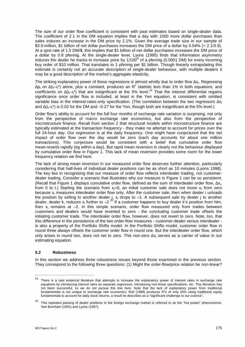
BIS Papers No 2 175
The size of our order flow coefficient is consistent with past estimates based on single-dealer data.The coefficient of 2.1 in the DM equation implies that a day with 1000 more dollar purchases thansales induces an increase in the DM price by 2.1%. Given the average trade size in our sample of$3.9 million, $1 billion of net dollar purchases increases the DM price of a dollar by 0.54% (= 2.1/3.9).At a spot rate of 1.5 DM/$, this implies that $1 billion of net dollar purchases increases the DM price ofa dollar by 0.8 pfennig. At the single-dealer level, Lyons (1995) finds that information asymmetryinduces the dealer he tracks to increase price by 1/100th of a pfennig (0.0001 DM) for every incomingbuy order of $10 million. That translates to 1 pfennig per $1 billion. Though linearly extrapolating thisestimate is certainly not an accurate description of single-dealer behaviour, with multiple dealers itmay be a good description of the market’s aggregate elasticity.
The striking explanatory power of these regressions is almost wholly due to order flow ∆xt. Regressing∆pt on ∆(it–it*) alone, plus a constant, produces an R2 statistic less than 1% in both equations, andcoefficients on ∆(it–it*) that are insignificant at the 5% level.19 That the interest differential regainssignificance once order flow is included, at least in the Yen equation, is consistent with omittedvariable bias in the interest-rates-only specification. (The correlation between the two regressors ∆xt
and ∆(it–it*) is 0.02 for the DM and –0.27 for the Yen, though both are insignificant at the 5% level.)
Order flow’s ability to account for the full four months of exchange rate variation is surprising, not onlyfrom the perspective of macro exchange rate economics, but also from the perspective ofmicrostructure finance. Recall from section 2 that structural models within microstructure finance aretypically estimated at the transaction frequency - they make no attempt to account for prices over thefull 24-hour day. Our regression is at the daily frequency. One might have conjectured that the netimpact of order flow over the day would be zero (each day accounts for about one milliontransactions). This conjecture would be consistent with a belief that cumulative order flowmean-reverts rapidly (eg within a day). But rapid mean reversion is clearly not the behaviour displayedby cumulative order flow in Figure 1. This lack of mean reversion provides some room for the lowerfrequency relation we find here.
The lack of strong mean reversion in our measured order flow deserves further attention, particularlyconsidering that half-lives of individual dealer positions can be as short as 10 minutes (Lyons 1998).The key lies in recognising that our measure of order flow reflects interdealer trading, not customer-dealer trading. Consider a scenario that illustrates why our measure in Figure 1 can be so persistent.(Recall that Figure 1 displays cumulative order flow, defined as the sum of interdealer order flow, ∆xt,from 0 to t.) Starting the scenario from xt=0, an initial customer sale does not move xt from zerobecause xt measures interdealer order flow only. After the customer sale, then when dealer i unloadsthe position by selling to another dealer j, xt drops to –1. A subsequent sale by dealer j to anotherdealer, dealer k, reduces xt further to –2.20 If a customer happens to buy dealer k’s position from him,then xt remains at –2. In this simple scenario, order flow measured only from trades betweencustomers and dealers would have reverted to zero - the concluding customer trade offsets theinitiating customer trade. The interdealer order flow, however, does not revert to zero. Note, too, thatthis difference in the persistence of the two order-flow measures - customer-dealer versus interdealer -is also a property of the Portfolio Shifts model. In the Portfolio Shifts model, customer order flow inround three always offsets the customer order flow in round one. But the interdealer order flow, whichonly arises in round two, does not net to zero. This non-zero ∆xt serves as a carrier of value in ourestimating equation.
5.2 Robustness
In this section we address three robustness issues beyond those examined in the previous section.They correspond to the following three questions: (1) Might the order-flow/price relation be non-linear?
19There is a vast empirical literature that attempts to increase the explanatory power of interest rates in exchange rateequations by introducing interest rates as separate regressors, introducing non-linear specifications, etc. This literature hasnot been successful, so we do not pursue this line here. Note that the lack of explanatory power from traditionalfundamentals is not unique to exchange rate economics: Roll (1988) produces R2s of only 20% using traditional equityfundamentals to account for daily stock returns, a result he describes as a “significant challenge to our science”.
20This repeated passing of dealer positions in the foreign exchange market is referred to as the “hot potato” phenomenon.See Burnham (1991) and Lyons (1997).

176 BIS Papers No 2
(2) Does the relation depend on the gross level of activity? and (3) Does the relation depend on day ofthe week?
Might the order-flow/price relation be non-linear?
The linearity of our Portfolio Shifts specification depends crucially on several simplifying assumptions,some of which are rather strong on empirical grounds. It is therefore natural to investigate whethernon-linearities or asymmetries might be present.21 A simple first test is to add a squared order-flowterm to the baseline specification. The squared order-flow term is insignificant in both equations. Wealso test whether the coefficient on order flow is piece-wise linear, with a kink at ∆xt=0. If true, thismeans that buying pressure and selling pressure are not symmetric. A Wald test that the two slopecoefficients are equal cannot be rejected for the DM equation. There is some evidence of differentslopes in the Yen equation however: the test is rejected at the 4% marginal significance level. In thatcase, the point estimates show a greater sensitivity of price to order flow in the downward direction,though both estimates remain positive and significant.
Does the order-flow/price relation depend on the gross level of activity?
Another natural concern is whether the order-flow/price relation in Table 1 is state contingent in someway, perhaps depending on the market’s overall activity level. Our data set provides a convenientmeasure of overall activity, namely the total number of transactions. As a simple test, we partition oursample of trading days into quartiles, from days with the fewest transactions to days with the mosttransactions. We then estimate separate order-flow coefficients for each of these four samplepartitions. In both the DM and Yen equations, all four of the order-flow coefficients are positive. In theDM equation, the coefficients are slightly U-shaped (from fewest transactions to most, the pointestimates for β2 are 2.7, 2.0, 1.9, and 3.3). In the Yen equation, the coefficients are monotonicallyincreasing (from fewest transactions to most, the point estimates for β2 are 1.0, 1.1, 3.5, and 4.1).
In terms of theory, this result for the Yen is consistent with the “event-uncertainty” model of Easley andO’Hara (1992), but the DM result is not. The event-uncertainty model predicts that trades are moreinformative when trading intensity is higher. Key to understanding their result is that in their model,new information may not exist. If there is trading at time t, then a rational dealer raises her conditionalprobability that an information event has occurred, and lowers the probability of the “no-information”event. The upshot is that trades occurring when trading intensity is high induce a larger update inbeliefs, and therefore a larger adjustment in price.
Does the order-flow/price relation depend on day of the week?
Another state-contingency that warrants attention is day-of-the-week effects.22 To test whether day-of-the-week matters, we partition our sample into five sub-samples, one for each weekday (recall thatweekends are subsumed in our Friday-to-Monday observations). In both the DM and Yen equations,all five of the resulting order-flow coefficients are positive. In the DM equation, the Tuesday coefficientis the largest, and the Wednesday coefficient is the smallest. The Yen equation also shows thatTuesday’s coefficient is the largest, but in this case the Monday coefficient is smallest. More important,a Wald test that the coefficients are equal across the five days cannot be rejected at the 5% level ineither equation (though in the case of the Yen, it can be rejected at the 10% level).
5.3 Causality
Under our model’s null hypothesis, causality runs strictly from order flow to price. Accordingly, underthe null, our estimation is not subject to simultaneity bias. (We are not simply “regressing price onquantity,” as in the classic supply-demand identification problem. Quantity - ie volume - and order floware fundamentally different concepts.) Within microstructure theory more broadly, this direction of
21We pursue these (simple) non-linear specifications with the comfort that outliers are not driving our results - a fact that ismanifest from Figure 1.
22In terms of theory, the model of Foster and Viswanathan (1990) is a workhorse for specifying day-of-the-week effects. Intheir model, there is periodic variation in the information advantage of the informed trader. This advantage is assumed togrow over periods of market closure, in particular, over weekends, making order flow on Monday particularly potent.

BIS Papers No 2 177
causality is the norm: it holds in all the canonical models (Glosten and Milgrom 1985, Kyle 1985, Stoll1978, Amihud and Mendelson 1980), despite the fact that price and order flow are determinedsimultaneously. The important point in these models is that price innovations are a function of orderflow innovations, not the other way around.23 That said, alternative hypotheses do exist under whichcausality is reversed. The following taxonomy frames the causality issue, and identifies specificalternatives under which causality is reversed, so that the merits of these alternatives can be judged ina disciplined way.
Theoretical overview
The timing of the order-flow/price relation admits three possibilities, depending on whether order flowprecedes, is concurrent with, or lags price adjustment. We shall refer to these three timing hypothesesas the Anticipation hypothesis, the Pressure hypothesis, and the Feedback hypothesis, respectively.
Within each of the three hypotheses - Anticipation, Pressure, and Feedback - there are also variations.Under the Anticipation hypothesis, for example, order flow can precede price adjustment becauseprices adjust fully only after order flow is commonly observed - in low-transparency markets likeforeign exchange, order flow is not commonly observed when it occurs (Lyons 1996). Order flow mightalso precede price because price adjusts only after some piece of news anticipated by order flow iscommonly observed (eg the short-lived private information in Foster and Viswanathan 1990). Underthe Pressure hypothesis the two main variations correspond to microstructure theory’s canonicalmodel types - information models and inventory models. In information models, observing order flowprovides information about payoffs (Glosten and Milgrom 1985, Kyle 1985). In inventory models, orderflow alters equilibrium risk premia (Stoll 1978, Ho and Stoll 1981).24 Under the Feedback hypothesis,order flow lags price because of feedback trading. Negative-feedback trading is systematic selling inresponse to price increases, and buying in response to price decreases (eg Friedman’s celebrated“stabilising speculators”). Positive-feedback trading is the reverse. Variations on the Feedbackhypothesis are distinguished by whether this feedback trading is rational (an optimal response toreturn autocorrelation) or behavioural, meaning that it arises from systematic decision bias (DeLong etal. 1990, Jegadeesh and Titman 1993, Grinblatt et al. 1995).
Under the Pressure hypothesis, causality runs from order flow to price, despite their concurrentrealisation.25 For the Anticipation hypothesis, the second variation noted above - where price adjustsonly after some piece of news anticipated by order flow is observed - is probably not relevant toforeign exchange (in contrast to equity markets, where insider order flow can anticipate a firm’searnings announcement, for example). The other variation of the Anticipation hypothesis - where orderflow affects price with a delay because it is not commonly observed - is relevant to foreign exchange.In this case, causality still runs from order flow to price, but the effects are delayed. As noted in theData section, order flow in this market is not common knowledge when realised. Consequently, lags inprice adjustment do not violate market efficiency (conditional on public information). One way to testthis variation of the Anticipation hypothesis is by introducing lagged order flow to our Portfolio Shiftsmodel. Rows one and three of Table 2 present the results of this regression: lagged order flow isinsignificant. At the daily frequency, lagged order flow is already embedded in price.26
23Put differently, order flow in these models is a proximate cause. The underlying driver of order flow is non-public information(information about uncertain demands, information about payoffs, etc). Order flow is the channel through which this type ofinformation is impounded in price.
24Within this inventory-model category, there is an additional distinction between price effects that arise at the marketmakerlevel (canonical inventory models) and price effects that arise at the marketwide level, due to imperfect substitutability(eg our Portfolio Shifts model). In the case of price effects at the marketmaker level, these effects are often modeled aschanging risk premia. But sometimes, largely for technical convenience, models are specified with risk-neutralmarketmakers who face some generic “inventory holding cost.”
25This does not imply that price cannot influence order flow. Price does influence order flow in microstructure models (both forthe usual downward sloping demand reason, and because agents learn from price). It is still the case that - in equilibrium -price innovations are functions of order flow innovations, not vice versa. Our Portfolio Shifts model is a case in point.
26As another check along these lines, we also decompose contemporaneous order flow into expected and unexpectedcomponents (by projecting it on past order flow). In our model, all order flow ∆x is unexpected, but this need not be the casein the data. We find, as the model predicts, that order flow’s explanatory power comes from its unexpected component.
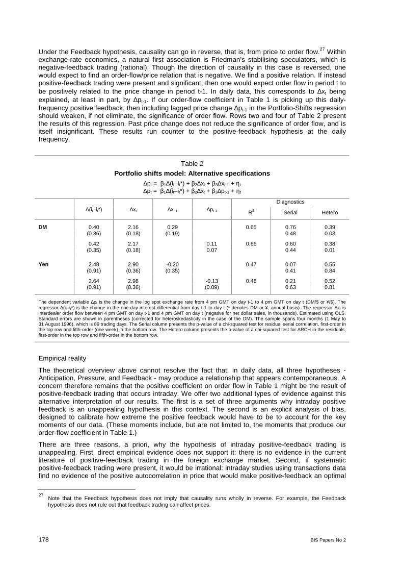
178 BIS Papers No 2
Under the Feedback hypothesis, causality can go in reverse, that is, from price to order flow.27 Withinexchange-rate economics, a natural first association is Friedman’s stabilising speculators, which isnegative-feedback trading (rational). Though the direction of causality in this case is reversed, onewould expect to find an order-flow/price relation that is negative. We find a positive relation. If insteadpositive-feedback trading were present and significant, then one would expect order flow in period t tobe positively related to the price change in period t-1. In daily data, this corresponds to ∆xt beingexplained, at least in part, by ∆pt-1. If our order-flow coefficient in Table 1 is picking up this daily-frequency positive feedback, then including lagged price change ∆pt-1 in the Portfolio-Shifts regressionshould weaken, if not eliminate, the significance of order flow. Rows two and four of Table 2 presentthe results of this regression. Past price change does not reduce the significance of order flow, and isitself insignificant. These results run counter to the positive-feedback hypothesis at the dailyfrequency.
Table 2
Portfolio shifts model: Alternative specifications∆pt = β1∆(it–it*) + β2∆xt + β3∆xt-1 + ηt
∆pt = β1∆(it–it*) + β2∆xt + β3∆pt-1 + ηt
Diagnostics∆(it–it*) ∆xt ∆xt-1 ∆pt-1 R2 Serial Hetero
DM 0.40 2.16 0.29 0.65 0.76 0.39(0.36) (0.18) (0.19) 0.48 0.03
0.42 2.17 0.11 0.66 0.60 0.38(0.35) (0.18) 0.07 0.44 0.01
Yen 2.48 2.90 -0.20 0.47 0.07 0.55(0.91) (0.36) (0.35) 0.41 0.84
2.64 2.98 -0.13 0.48 0.21 0.52(0.91) (0.36) (0.09) 0.63 0.81
The dependent variable ∆pt is the change in the log spot exchange rate from 4 pm GMT on day t-1 to 4 pm GMT on day t (DM/$ or ¥/$). Theregressor ∆(it–it*) is the change in the one-day interest differential from day t-1 to day t (* denotes DM or ¥, annual basis). The regressor ∆xt isinterdealer order flow between 4 pm GMT on day t-1 and 4 pm GMT on day t (negative for net dollar sales, in thousands). Estimated using OLS.Standard errors are shown in parentheses (corrected for heteroskedasticity in the case of the DM). The sample spans four months (1 May to31 August 1996), which is 89 trading days. The Serial column presents the p-value of a chi-squared test for residual serial correlation, first-order inthe top row and fifth-order (one week) in the bottom row. The Hetero column presents the p-value of a chi-squared test for ARCH in the residuals,first-order in the top row and fifth-order in the bottom row.
Empirical reality
The theoretical overview above cannot resolve the fact that, in daily data, all three hypotheses -Anticipation, Pressure, and Feedback - may produce a relationship that appears contemporaneous. Aconcern therefore remains that the positive coefficient on order flow in Table 1 might be the result ofpositive-feedback trading that occurs intraday. We offer two additional types of evidence against thisalternative interpretation of our results. The first is a set of three arguments why intraday positivefeedback is an unappealing hypothesis in this context. The second is an explicit analysis of bias,designed to calibrate how extreme the positive feedback would have to be to account for the keymoments of our data. (These moments include, but are not limited to, the moments that produce ourorder-flow coefficient in Table 1.)
There are three reasons, a priori, why the hypothesis of intraday positive-feedback trading isunappealing. First, direct empirical evidence does not support it: there is no evidence in the currentliterature of positive-feedback trading in the foreign exchange market. Second, if systematicpositive-feedback trading were present, it would be irrational: intraday studies using transactions datafind no evidence of the positive autocorrelation in price that would make positive-feedback an optimal
27Note that the Feedback hypothesis does not imply that causality runs wholly in reverse. For example, the Feedbackhypothesis does not rule out that feedback trading can affect prices.

BIS Papers No 2 179
response (Goodhart, Ito, and Payne 1996). Third, the fallback possibility of irrational positive-feedbacktrading is difficult to defend. Recall that the order flow we measure is interdealer order flow. Thoughsystematic feedback trading of a behavioural nature (ie not fully rational) might be a good descriptionof some market participants, dealers are among the most sophisticated participants in this market.
Bias analysis
To close this section on causality, let us consider what it would take for positive-feedback trading toaccount for our results. Specifically, suppose intraday positive-feedback trading is present - Underwhat conditions could it account for the key moments of our data? These moments include, but are notlimited to, the moments that produce our positive order-flow coefficient in Table 1. We show below thatthese conditions are rather extreme. In fact, through a broad range of underlying parameter values,feedback trading would have to be negative to account for the key moments of our data.
We start by decomposing measured order flow ∆xt into two components:
(8) ∆xt = ∆xt1 + ∆xt2
where ∆xt1 denotes exogenous order flow from portfolio shifts (a la our model), with variance equal toΣx1, and ∆xt2 denotes order flow due to feedback trading, where
(9) ∆xt2 = γ∆pt
Suppose the true structural model can be written as:
(10) ∆pt = α∆xt1 + εt
where εt represents common-knowledge (CK) news, and εt is iid with variance Σε. By CK news wemean that both the information and its implication for equilibrium price is common knowledge. If bothconditions are not met, then order flow will convey information about market-clearing prices (recall thediscussion in the introduction). If feedback trading is present (γ≠0), then α will be a reduced formcoefficient that depends on γ. Note that under these circumstances, equation (10) is a valid reduced-from equation that could be estimated by OLS if one had data on ∆xt1.
With data on ∆xt and ∆pt only, suppose we estimate
(11) ∆pt = β∆xt + εt
If γ≠0, our estimates of β will suffer from simultaneity bias. To evaluate the size of this bias, considerthe implications of equations (8) through (10) for the moments:
β = Cov(∆pt,∆xt) / Var(∆xt)
δ = Var(∆pt) / Var(∆xt)
From equations (8) through (10) we know that:
∆xt = (1+γα)(∆xt1) + γεt
Solving for expressions for Cov(∆pt,∆xt), Var(∆pt), and Var(∆xt), we can write:
β = Cov(∆pt,∆xt) / Var(∆xt) = (α(1+γα)Σx1 + γΣε) / ((1+γα)2Σx1 + γ2Σε)
δ = Var(∆pt) / Var(∆xt) = (α2Σx1 + Σε) / ((1+γα)2Σx1 + γ2Σε)Now, define an additional parameter:
φ = Σε/Σx1
This parameter represents the ratio of CK news to order-flow news. With this parameter φ we canrewrite the key coefficients as:
β = (α(1+γα) + γφ) / ((1+γα)2 + γ2φ)
δ = (α2 + φ) / ((1+γα)2
+ γ2φ)
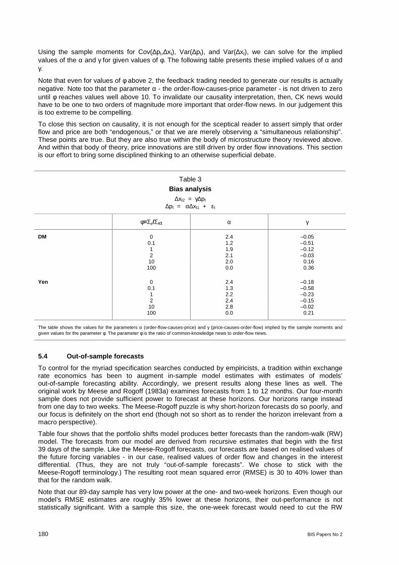
180 BIS Papers No 2
Using the sample moments for Cov(∆pt,∆xt), Var(∆pt), and Var(∆xt), we can solve for the impliedvalues of the α and γ for given values of φ. The following table presents these implied values of α andγ.
Note that even for values of φ above 2, the feedback trading needed to generate our results is actuallynegative. Note too that the parameter α - the order-flow-causes-price parameter - is not driven to zerountil φ reaches values well above 10. To invalidate our causality interpretation, then, CK news wouldhave to be one to two orders of magnitude more important that order-flow news. In our judgement thisis too extreme to be compelling.
To close this section on causality, it is not enough for the sceptical reader to assert simply that orderflow and price are both “endogenous,” or that we are merely observing a “simultaneous relationship”.These points are true. But they are also true within the body of microstructure theory reviewed above.And within that body of theory, price innovations are still driven by order flow innovations. This sectionis our effort to bring some disciplined thinking to an otherwise superficial debate.
Table 3
Bias analysis∆xt2 = γ∆pt
∆pt = α∆xt1 + εt
φ=Σε/Σx1 α γ
DM 0 2.4 –0.050.1 1.2 –0.511 1.9 –0.122 2.1 –0.0310 2.0 0.16
100 0.0 0.36
Yen 0 2.4 –0.180.1 1.3 –0.581 2.2 –0.232 2.4 –0.1510 2.8 –0.02
100 0.0 0.21
The table shows the values for the parameters α (order-flow-causes-price) and γ (price-causes-order-flow) implied by the sample moments andgiven values for the parameter φ. The parameter φ is the ratio of common-knowledge news to order-flow news.
5.4 Out-of-sample forecasts
To control for the myriad specification searches conducted by empiricists, a tradition within exchangerate economics has been to augment in-sample model estimates with estimates of models’out-of-sample forecasting ability. Accordingly, we present results along these lines as well. Theoriginal work by Meese and Rogoff (1983a) examines forecasts from 1 to 12 months. Our four-monthsample does not provide sufficient power to forecast at these horizons. Our horizons range insteadfrom one day to two weeks. The Meese-Rogoff puzzle is why short-horizon forecasts do so poorly, andour focus is definitely on the short end (though not so short as to render the horizon irrelevant from amacro perspective).
Table four shows that the portfolio shifts model produces better forecasts than the random-walk (RW)model. The forecasts from our model are derived from recursive estimates that begin with the first39 days of the sample. Like the Meese-Rogoff forecasts, our forecasts are based on realised values ofthe future forcing variables - in our case, realised values of order flow and changes in the interestdifferential. (Thus, they are not truly “out-of-sample forecasts”. We chose to stick with theMeese-Rogoff terminology.) The resulting root mean squared error (RMSE) is 30 to 40% lower thanthat for the random walk.
Note that our 89-day sample has very low power at the one- and two-week horizons. Even though ourmodel’s RMSE estimates are roughly 35% lower at these horizons, their out-performance is notstatistically significant. With a sample this size, the one-week forecast would need to cut the RW
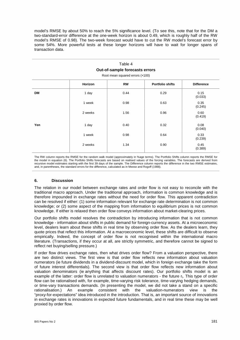
BIS Papers No 2 181
model’s RMSE by about 50% to reach the 5% significance level. (To see this, note that for the DM atwo-standard-error difference at the one-week horizon is about 0.49, which is roughly half of the RWmodel’s RMSE of 0.98). The two-week forecast would have to cut the RW model’s forecast error bysome 54%. More powerful tests at these longer horizons will have to wait for longer spans oftransaction data.
Table 4
Out-of-sample forecasts errorsRoot mean squared errors (×100)
Horizon RW Portfolio shifts Difference
DM 1 day 0.44 0.29 0.15(0.033)
1 week 0.98 0.63 0.35(0.245)
2 weeks 1.56 0.96 0.60(0.419)
Yen 1 day 0.40 0.32 0.08(0.040)
1 week 0.98 0.64 0.33(0.239)
2 weeks 1.34 0.90 0.45(0.389)
The RW column reports the RMSE for the random walk model (approximately in %age terms). The Portfolio Shifts column reports the RMSE forthe model in equation (6). The Portfolio Shifts forecasts are based on realised values of the forcing variables. The forecasts are derived fromrecursive model estimates starting with the first 39 days of the sample. The Difference column reports the difference in the two RMSE estimates,and, in parentheses, the standard errors for the difference, calculated as in Meese and Rogoff (1988).
6. Discussion
The relation in our model between exchange rates and order flow is not easy to reconcile with thetraditional macro approach. Under the traditional approach, information is common knowledge and istherefore impounded in exchange rates without the need for order flow. This apparent contradictioncan be resolved if either: (1) some information relevant for exchange rate determination is not commonknowledge; or (2) some aspect of the mapping from information to equilibrium prices is not commonknowledge. If either is relaxed then order flow conveys information about market-clearing prices.
Our portfolio shifts model resolves the contradiction by introducing information that is not commonknowledge - information about shifts in public demand for foreign-currency assets. At a microeconomiclevel, dealers learn about these shifts in real time by observing order flow. As the dealers learn, theyquote prices that reflect this information. At a macroeconomic level, these shifts are difficult to observeempirically. Indeed, the concept of order flow is not recognised within the international macroliterature. (Transactions, if they occur at all, are strictly symmetric, and therefore cannot be signed toreflect net buying/selling pressure.)
If order flow drives exchange rates, then what drives order flow? From a valuation perspective, thereare two distinct views. The first view is that order flow reflects new information about valuationnumerators (ie future dividends in a dividend-discount model, which in foreign exchange take the formof future interest differentials). The second view is that order flow reflects new information aboutvaluation denominators (ie anything that affects discount rates). Our portfolio shifts model is anexample of the latter: order flow is unrelated to valuation numerators - the future rt. This type of orderflow can be rationalised with, for example, time-varying risk tolerance, time-varying hedging demands,or time-vary transactions demands. (In presenting the model, we did not take a stand on a specificrationalisation.) An example consistent with the valuation-numerators view is the“proxy-for-expectations” idea introduced in the introduction. That is, an important source of innovationsin exchange rates is innovations in expected future fundamentals, and in real time these may be wellproxied by order flow.

182 BIS Papers No 2
Note that separating valuation numerators from valuation denominators has implications for theconcept of “fundamentals.” Order flow that reflects information about valuation numerators - likeexpectations of future interest rates - is in keeping with traditional definitions of exchange-ratefundamentals. But order flow that reflects valuation denominators encompasses nontraditionalexchange-rate determinants, calling, perhaps for a broader definition. In any event, exploring theselinks to deeper determinants is a natural topic for future research. This will surely require a retreatback into intraday data.28
The practitioner view versus the academic view
Another perspective on order flow emerges from the difference between academic and practitionerviews on price determination. Practitioners often explain price increases with the familiar reasoningthat “there were more buyers than sellers.” To most economists, this reasoning is tantamount to “pricehad to rise to balance demand and supply.” But these phrases may not be equivalent. For economists,the phrase “price had to rise to balance demand and supply” calls to mind the Walrasian auctioneer.The Walrasian auctioneer collects “preliminary” orders and uses them to find the market-clearing price.Importantly, the auctioneer’s price adjustment is immediate - no trading occurs in the transition. (In arational-expectations model of trading, for example, this is manifested in all orders being conditionedon the market-clearing price.)
Many practitioners have a different model in mind. In the practitioner model there is a dealer instead ofan abstract auctioneer. The dealer acts as a buffer between buyers and sellers. The orders the dealercollects are actual orders, rather than preliminary orders, so trading does occur in the transition to thenew price. The dealer determines new prices from the new information about demand and supply thatbecomes available.
Can the practitioner model be rationalised? At first blush, it appears that trades are taking place out ofequilibrium, implying irrational behaviour. But this misses an important piece of the puzzle. Whetherthese trades are out-of-equilibrium depends on the information available to the dealer. If the dealerknows at the outset that there are more buyers than sellers (eventually pushing price up), then it maynot be optimal to sell at a low interim price. If the buyer/seller imbalance is not known, however, thenrational trades can occur through the transition. In this case, the dealer cannot set price conditional onall the information available to the Walrasian auctioneer. This is precisely the story developed incanonical microstructure models (Glosten and Milgrom 1985). Trading that would be irrational if thedealer could condition on the auctioneer’s information can be rationalised in models with more limited(and realistic) conditioning information.
Relation between our model and the flow approach to exchange rates
Consider the relation between our model, with its emphasis on order flow, and the traditional “flowapproach” to exchange rates. Is our approach just a return to the earlier flow approach? Despite theirapparent similarity, the two approaches are distinct and, in fact, fundamentally different.
A key feature of our model is that order flow plays two roles. First, holding beliefs constant, order flowaffects price through the traditional process of market clearing. Second, order flow also alters beliefsbecause it conveys information that is not yet common knowledge. That is:
Price = P(∆x, B(∆x,…), …)
Price P thus depends both directly and indirectly on order flow, ∆x, where the indirect effect is viabeliefs B. Early attempts to analyse equilibrium with differentially informed individuals ignored theinformation role - the effect of order flow on beliefs. Since the advent of rational expectations, modelsthat ignore this information effect from order flow are viewed as less compelling.
28The role of macro announcements in determining order flow warrants exploring. This, too, requires the use of intraday data.A second possible use of macro announcements is to introduce them directly into our Portfolio Shifts specification, even atthe daily frequency. This tack is not likely to be fruitful: there is a long literature showing that macro announcements areunable to account for exchange rate first moments (as opposed to second moments; see Andersen and Bollerslev 1998).
BIS Papers No 2 183
This is the essential difference between the flow approach to exchange rates and the microstructureapproach. Under the flow approach, order flow communicates no information back to individualsregarding others’ views/information. All information is common knowledge, so there is no informationthat needs aggregating. Under the microstructure approach, order flow does communicate informationthat is not common knowledge. This information needs to be aggregated by the market, andmicrostructure theory describes how that aggregation is achieved, depending on the underlyinginformation type.
7. Conclusion
This paper presents a model of exchange rate determination of a new kind. Instead of relyingexclusively on macroeconomic determinants, we draw on determinants from the field ofmicrostructure. In particular, we focus on order flow, the variable within microstructure that is - boththeoretically and empirically - the driver of price.29 This is a radical departure from traditionalapproaches to exchange rate determination. Traditional approaches, with their common-knowledgeenvironments, admit no role for information aggregation. Our findings suggest instead that the problemthis market solves is indeed one of information aggregation.
Our Portfolio Shifts model provides an explicit characterisation of this information aggregationproblem. The model is also strikingly successful in accounting for realised rates. It accounts for morethan 60% of daily changes in the DM/$ rate, and more than 40% of daily changes in the Yen/$ rate.Out of sample, our model produces better short-horizon forecasts than a random walk. Our estimatesof the sensitivity of the spot rate to order flow are sensible as well, and square with past estimates atthe individual-dealer level. We find that for the DM/$ market as a whole, $1 billion of net dollarpurchases increases the DM price of a dollar by about 0.5%. This relation should be of particularinterest to people working on central bank intervention (though care should be exercised in mappingcentral bank orders to subsequent interdealer trades).
Two issues raised by our measure of order flow deserve some remarks. First, though our measurecaptures a substantial share of total trading, it remains incomplete. As data sets covering customer-dealer trading and brokered interdealer trading become available, the order-flow picture can becompleted (see, eg Payne 1999). A second interesting issue raised by our order-flow measure iswhether its relation to price would change if order flow were observable to dealers in real time (ie if themarket were more transparent). From a policy perspective, the effects of increasing order-flowtransparency may be important: unlike most other financial markets, the FX market is unregulated inthis respect. The welfare consequences are not yet well understood.
So where do the results of this paper lead us? In our judgement they point toward a research agendathat borrows from both the macro and microstructure approaches. It is not necessary to decoupleexchange rates from macroeconomic fundamentals, as is common within microstructure finance. Inthis way, the approach is more firmly anchored in the broader context of asset pricing. (Though wefreely admit that longer time series will be necessary to implement the macro dimension fully.) Nor is itnecessary to treat exchange rates as driven wholly by public information, as is common within themacro approach. The information aggregation that arises when one reduces reliance on publicinformation is well suited to microstructure: there are ample tools within the microstructure approachfor addressing this aggregation. In the end, this two-pronged approach may help locate the missingmiddle in exchange rate economics - that disturbing space between our successful modelling of veryshort and very long horizons.
We close by addressing the obvious challenge for this agenda: What drives order flow? Here are twostrategies, among many, for shedding light on this question. The first strategy involves disaggregatingorder flow. For example, interdealer order flow can be split into large banks versus small banks, orinvestment banks versus commercial banks. Data sets on customer order flow can be split into non-financial corporations, leveraged financial institutions (eg hedge funds), and unleveraged financialinstitutions (eg mutual and pension funds). Do all these trade types have the same price impact? Ifnot, whose trades are most informative? This will clarify the underlying sources of non-CK information,
29This primacy of order flow within microstructure should mitigate standard concerns about data snooping. (In the words ofRichard Meese 1990, “At this point exchange rate modelers can be justly accused of in-sample data mining.”) The variablewe introduce - order flow - is the obvious a priori driving variable from microstructure theory.

184 BIS Papers No 2
which brings us closer to a specification of this market’s information structure. The second strategyinvolves focusing on periods where we expect CK information to be most important, for example,periods encompassing scheduled macro announcements. Does order flow account for a smaller shareof the price variation within these periods? Or is order flow an important channel for resolvinguncertainty about the mapping from public information to price? Whatever the result, the importantpoint is that the what-drives-order-flow question is not beyond our grasp.
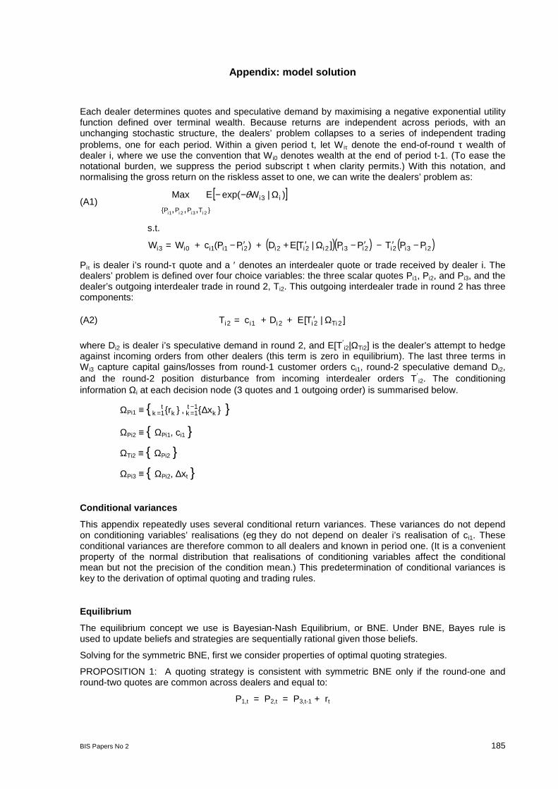
BIS Papers No 2 185
Appendix: model solution
Each dealer determines quotes and speculative demand by maximising a negative exponential utilityfunction defined over terminal wealth. Because returns are independent across periods, with anunchanging stochastic structure, the dealers’ problem collapses to a series of independent tradingproblems, one for each period. Within a given period t, let Wiτ denote the end-of-round τ wealth ofdealer i, where we use the convention that Wi0 denotes wealth at the end of period t-1. (To ease thenotational burden, we suppress the period subscript t when clarity permits.) With this notation, andnormalising the gross return on the riskless asset to one, we can write the dealers’ problem as:
(A1)[ ]
3
2321 ,,,
)|exp(
iiii TPPP
iiWEMax Ω−− θ
s.t.
( )( ) ( )2322322221103 ]|[)( iiiiiiiiiiiii PPTPPTEDPPcWW −′−′−Ω′++′−+=
Piτ is dealer i’s round-τ quote and a ′ denotes an interdealer quote or trade received by dealer i. Thedealers’ problem is defined over four choice variables: the three scalar quotes Pi1, Pi2, and Pi3, and thedealer’s outgoing interdealer trade in round 2, Ti2. This outgoing interdealer trade in round 2 has threecomponents:
(A2) ]|[ 22212 Tiiiii TEDcT Ω′++=
where Di2 is dealer i’s speculative demand in round 2, and E[T′i2|ΩTi2] is the dealer’s attempt to hedge
against incoming orders from other dealers (this term is zero in equilibrium). The last three terms inWi3 capture capital gains/losses from round-1 customer orders ci1, round-2 speculative demand Di2,and the round-2 position disturbance from incoming interdealer orders T′
i2. The conditioninginformation Ωi at each decision node (3 quotes and 1 outgoing order) is summarised below.
ΩPi1 ≡ 1 kt
k r= , 11 k
tk x∆−
=
ΩPi2 ≡ ΩPi1, ci1
ΩTi2 ≡ ΩPi2
ΩPi3 ≡ ΩPi2, ∆xt
Conditional variances
This appendix repeatedly uses several conditional return variances. These variances do not dependon conditioning variables’ realisations (eg they do not depend on dealer i’s realisation of ci1. Theseconditional variances are therefore common to all dealers and known in period one. (It is a convenientproperty of the normal distribution that realisations of conditioning variables affect the conditionalmean but not the precision of the condition mean.) This predetermination of conditional variances iskey to the derivation of optimal quoting and trading rules.
Equilibrium
The equilibrium concept we use is Bayesian-Nash Equilibrium, or BNE. Under BNE, Bayes rule isused to update beliefs and strategies are sequentially rational given those beliefs.
Solving for the symmetric BNE, first we consider properties of optimal quoting strategies.
PROPOSITION 1: A quoting strategy is consistent with symmetric BNE only if the round-one andround-two quotes are common across dealers and equal to:
P1,t = P2,t = P3,t-1 + rt
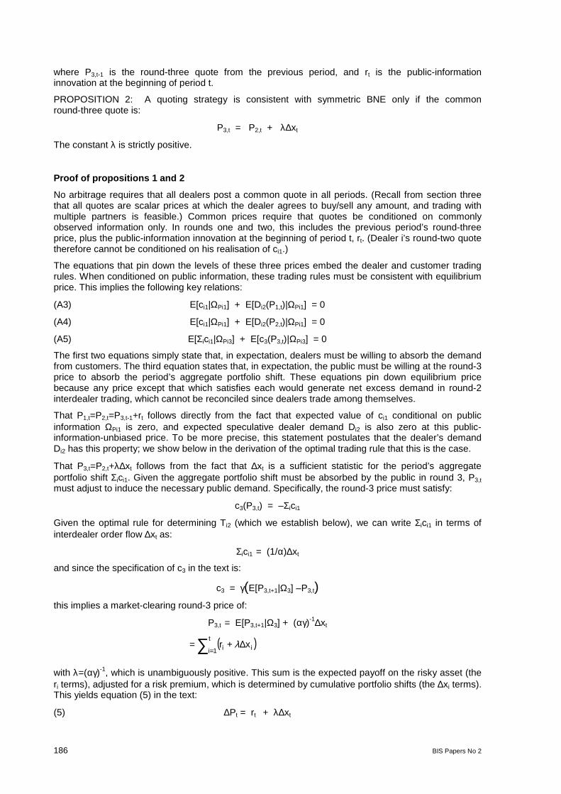
186 BIS Papers No 2
where P3,t-1 is the round-three quote from the previous period, and rt is the public-informationinnovation at the beginning of period t.
PROPOSITION 2: A quoting strategy is consistent with symmetric BNE only if the commonround-three quote is:
P3,t = P2,t + λ∆xt
The constant λ is strictly positive.
Proof of propositions 1 and 2
No arbitrage requires that all dealers post a common quote in all periods. (Recall from section threethat all quotes are scalar prices at which the dealer agrees to buy/sell any amount, and trading withmultiple partners is feasible.) Common prices require that quotes be conditioned on commonlyobserved information only. In rounds one and two, this includes the previous period’s round-threeprice, plus the public-information innovation at the beginning of period t, rt. (Dealer i’s round-two quotetherefore cannot be conditioned on his realisation of ci1.)
The equations that pin down the levels of these three prices embed the dealer and customer tradingrules. When conditioned on public information, these trading rules must be consistent with equilibriumprice. This implies the following key relations:
(A3) E[ci1|ΩPi1] + E[Di2(P1,t)|ΩPi1] = 0
(A4) E[ci1|ΩPi1] + E[Di2(P2,t)|ΩPi1] = 0
(A5) E[Σici1|ΩPi3] + E[c3(P3,t)|ΩPi3] = 0
The first two equations simply state that, in expectation, dealers must be willing to absorb the demandfrom customers. The third equation states that, in expectation, the public must be willing at the round-3price to absorb the period’s aggregate portfolio shift. These equations pin down equilibrium pricebecause any price except that which satisfies each would generate net excess demand in round-2interdealer trading, which cannot be reconciled since dealers trade among themselves.
That P1,t=P2,t=P3,t-1+rt follows directly from the fact that expected value of ci1 conditional on publicinformation ΩPi1 is zero, and expected speculative dealer demand Di2 is also zero at this public-information-unbiased price. To be more precise, this statement postulates that the dealer’s demandDi2 has this property; we show below in the derivation of the optimal trading rule that this is the case.
That P3,t=P2,t+λ∆xt follows from the fact that ∆xt is a sufficient statistic for the period’s aggregateportfolio shift Σici1. Given the aggregate portfolio shift must be absorbed by the public in round 3, P3,t
must adjust to induce the necessary public demand. Specifically, the round-3 price must satisfy:
c3(P3,t) = –Σici1
Given the optimal rule for determining Ti2 (which we establish below), we can write Σici1 in terms ofinterdealer order flow ∆xt as:
Σici1 = (1/α)∆xt
and since the specification of c3 in the text is:
c3 = γ(E[P3,t+1|Ω3] –P3,t)this implies a market-clearing round-3 price of:
P3,t = E[P3,t+1|Ω3] + (αγ)-1∆xt
= ( )∑=∆+
t
1i ii xr λ
with λ=(αγ)-1, which is unambiguously positive. This sum is the expected payoff on the risky asset (theri terms), adjusted for a risk premium, which is determined by cumulative portfolio shifts (the ∆xi terms).This yields equation (5) in the text:
(5) ∆Pt = rt + λ∆xt

BIS Papers No 2 187
where ∆Pt denotes the change in price from the end of round three in period t-1 to the end of roundthree in period t.
Equilibrium trading strategies
An implication of common interdealer quotes P2,t is that in round two each dealer receives a share1/(N-1) of every other dealer’s interdealer trade. This order corresponds to the position disturbance T′
i2
in the dealer’s problem in equation (A1). Given the quoting strategy described in propositions one andtwo, the following trading strategy is optimal and corresponds to symmetric linear equilibrium:
PROPOSITION 3: The trading strategy profile:
Ti2 = α ci1
∀ i ∈ 1,...,N, with α>0, conforms to a Bayesian-Nash equilibrium.
Proof of proposition 3: optimal trading strategies
As noted above, because returns are independent across periods, with an unchanging stochasticstructure, the dealers’ problem collapses to a series of independent trading problems, one for eachperiod. Because there are only N dealers, however, each dealer acts strategically in the sense that hisspeculative demand depends on the impact his trade will have on subsequent prices.
It is well known that if a random variable W is distributed N(µ,σ2) and the utility function U(W)= –exp(–θW), then:
(A6) E[U(W)] = –exp[–θ(µ – θσ2/2)]Maximising E[U(W)] is therefore equivalent to maximising (µ – θσ2/2). This result allows us to write thedealers speculative-demand problem as:
(A7) Max i2D (E[P3|ΩTi2]–P2) – 2i2D (θ/2)σ2
Di2
where the information set ΩTi2 is defined above, and σ2 denotes the conditional variance of E[P3|ΩTi2]–P2. Now, from Proposition two, we can write:
(A8) E[P3|ΩTi2] – P2 = E[λ∆x|ΩTi2]
And from the definitions of ΩTi2 and ∆x we know that:
(A9) E[λ∆x|ΩTi2] = λTi2
The expected value of the other dealers’ trades in ∆x is 0 under our specification because (i) customertrades are mean-zero and independent across dealers and (ii) there is no information in the modelother than customer trades to motivate speculative demand. This fact also implies that dealer i’s tradein round 2, Ti2 from equation (A2), is equal to:
Ti2 = Di2 + ci1
Therefore, we can write the dealer’s problem as:
(A10) Max i2D λ(Di2 + ci1) – 2i2D (θ/2)σ2
Di2
The first-order condition of this problem is:
(A11) 2λDi2 + ci1 – θσ2Di2 = 0
which implies a speculative demand of:
(A12) 1222
1ii cD
−=
λθσ

188 BIS Papers No 2
This demand function and the fact that Ti2=Di2+ci1 imply:
(A13) 1122 12
1iii ccT α
λθσ≡
+
−=
The second-order condition for a maximum, (2λ–θσ2)<0, insures that α>0.
References
Amihud, Y and H Mendelson 1980, “Dealership market: Marketmaking with inventory”, Journal ofFinancial Economics, 8: 31-53.
Andersen, T and T Bollerslev 1998, “Deutsche mark-dollar volatility: Intraday activity patterns,macroeconomic announcements, and longer run dependencies”, Journal of Finance, 53: 219-266.
Bagwell, L 1992 “Dutch auction repurchases: An analysis of shareholder heterogeneity”, Journal ofFinance, 47: 71-105.
Bjonnes, G and D Rime 1998, “FX trading ... live: Impact of new trading environments, typescript”,Norwegian School of Management, December.
Blanchard, O 1979 “Speculative bubbles, crashes, and rational expectations”, Economics Letters, 14:387-389.
Burnham, J 1991 “Current structure and recent developments in foreign exchange markets, in S.Khoury” (ed.), Recent Developments in International Banking and Finance (North Holland,Amsterdam), 123-153.
Cai, J, Y Cheung, R Lee and M Melvin 1999, “Once-in-a-generation yen volatility in 1998:Fundamentals, intervention, or order flow?” typescript, Arizona State University, July.
Cheung, Y and M Chinn 1998 “Macroeconomic implications of the beliefs and behaviour of foreignexchange traders”, typescript, U.C. Santa Cruz, November.
Cheung, Y and C Wong 1998 “A survey of market practitioners’ views on exchange rate dynamics”,Journal of International Economics, forthcoming.
Chinn, M 1991 “Some linear and non-linear thoughts on exchange rates”, Journal of InternationalMoney and Finance, 10: 214-230.
Chinn, M and R Meese, 1994, “Banking on currency forecasts”, Journal of International Economics,38: 161-178.
Covrig, V and M Melvin 1998, “Asymmetric information and price discovery in the FX market: DoesTokyo know more about the yen?”, typescript, Arizona State University.
Degennaro, R and R Shrieves, 1997, “Public information releases, private information arrival, andvolatility in the foreign exchange market”, Journal of Empirical Finance, 4: 295-315.
DeLong, B, A Shleifer, L Summers and R Waldmann, 1990, “Positive feedback investment strategies,and destabilising rational speculation”, Journal of Finance, 45, 379-396.
Dominguez, K 1986, “Are foreign exchange forecasts rational?” New evidence from survey data,Economic Letters, 21: 277-281.
Dornbusch, R 1976, “Expectations and exchange rate dynamics”, Journal of Political Economy, 84:1161-1176.
Dornbusch, R 1982, “Equilibrium and disequilibrium exchange rates”, Zeitschrift fur Wirtschafts undSozialwissenschaften, 102: 573-799; reprinted in R. Dornbusch, Dollars, Debts and Deficits, MITPress: Cambridge, MA.
Easley, D and M O’Hara, 1992, “Time and the process of security price adjustment”, Journal ofFinance, 47: 577-605.
Evans, G 1986, “A test for speculative bubbles in the sterling-dollar exchange rate”, AmericanEconomic Review, 76: 621-636.

BIS Papers No 2 189
Evans, M 1997, “The microstructure of foreign exchange dynamics”, Georgetown University typescript,November, presented at the NBER Market Microstructure Conference, December 4, 1997.
Evans, M 1999, “What are the origins of foreign exchange movements?”, Georgetown Universitytypescript, March.
Fair, R 1970, “Estimation of simultaneous equations models with lagged endogenous variables andfirst order serially correlated errors”, Econometrica, 38: 507-516.
Flood, M 1994, “Market structure and inefficiency in the foreign exchange market”, Journal ofInternational Money and Finance, 13: 131-158.
Flood, R and R Hodrick, “On testing for speculative bubbles”, Journal of Economic Perspectives, 4:85-101.
Flood, R and A Rose, Fixing exchange rates: “A virtual quest for fundamentals”, Journal of MonetaryEconomics 36, 3-37.
Flood, R and M Taylor, 1996, “Exchange rate economics: What’s wrong with the conventional macroapproach?”, in Frankel, J G Galli and A Giovannini, (eds) The Microstructure of Foreign ExchangeMarkets (Chicago: The University of Chicago Press), 261-294.
Foster, D and S Viswanathan, 1990, “A theory of interday variations in volumes, variances, and tradingcosts in securities markets”, Review of Financial Studies, 3: 593-624.
Frankel, J and K Froot 1987, “Using survey data to test standard propositions regarding exchange rateexpectations”, American Economic Review, 77: 133-153.
Frankel, J, G Galli and A Giovannini 1996, “Introduction in The Microstructure of Foreign ExchangeMarkets” (Chicago: The University of Chicago Press), 1-15.
Frankel, J and A Rose 1995, “Empirical research on nominal exchange rates”, in G. Grossman and K.Rogoff (eds.), Handbook of International Economics, Elsevier Science: Amsterdam, 1689-1729.
Frenkel, J 1976, “A monetary approach to the exchange rate”: Doctrinal aspects and empiricalevidence, Scandinavian Journal of Economics, 78: 200-224.
Glosten, L and P Milgrom, 1985, “Bid, ask, and transaction prices in a specialist market withheterogeneously informed agents”, Journal of Financial Economics, 14: 71-100.
Goldberg, L and R Tenorio, 1997, “Strategic trading in a two-sided foreign exchange auction”, Journalof International Economics, 42: 299-326.
Goodhart, C 1988, “The foreign exchange market: A random walk with a dragging anchor”,Economica, 55: 437-460.
Goodhart, C, T Ito, and R Payne, 1996, “One day in June 1993”: A study of the working of the Reuters2000-2 electronic foreign exchange trading system. In The Microstructure of Foreign ExchangeMarkets, eds J Frankel, G Galli and A Giovannini, pp 107-179. University of Chicago Press, Chicago,IL.
Goodhart, C and M O’Hara 1997, “High frequency data in financial markets: Issues and applications”,Journal of Empirical Finance, 4: 73-114.
Grinblatt, M, S Titman and R Wermers, 1995, “Momentum investment strategies, portfolioperformance, and herding: A study of mutual fund behavior”, American Economic Review, 85, 1088-1105.
Hansch, O, N Naik and S Viswanathan 1998. “Do Inventories Matter in Dealership Markets? Evidencefrom the London Stock Exchange,” Journal of Finance, 53: 1623-1656.
Hau, H 1998, “Competitive entry and endogenous risk in the foreign exchange market”, Review ofFinancial Studies, 11: 757-788.
Ho, T and H Stoll, 1981, “Optimal dealer pricing under transactions and return uncertainty”, Journal ofFinancial Economics, 9, 47-73.
Hsieh, D and A Kleidon 1996, “Bid-ask spreads in foreign exchange markets: Implications for modelsof asymmetric information”, in Jeffrey Frankel et al eds: The Microstructure of Foreign ExchangeMarkets (University of Chicago Press, Chicago) 41-65.

190 BIS Papers No 2
Isard, P 1995, “Exchange Rate Economics”, Cambridge University Press: Cambridge, UK.
Ito, T, R Lyons and M Melvin, 1998, “Is there private information in the FX market?” The Tokyoexperiment, Journal of Finance 53, 1111-1130.
Jegadeesh, N and S Titman, 1993, “Returns to buying winners and selling losers: Implications forstock market efficiency”, Journal of Finance, 48, 65-92.
Jones, C, G Kaul and M Lipson, 1994, “Transactions, volume, and volatility”, Review of FinancialStudies, 7: 631-651.
Kouri, P 1976, “The exchange rate and the balance of payments in the short run and in the long run: Amonetary approach”, Scandinavian Journal of Economics, 78, 280-304.
Kouri, P and M Porter, 1974, “International capital flows and portfolio equilibrium”, Journal of PoliticalEconomy, 82, 443-467.
Kyle, A 1985, “Continuous auctions and insider trading”, Econometrica 53, 1315-1335.
Lyons, R 1995, “Tests of microstructural hypotheses in the foreign exchange market”, Journal ofFinancial Economics 39, 321-351.
Lyons, R 1996, “Optimal transparency in a dealer market with an application to foreign exchange”,Journal of Financial Intermediation, 5, 225-254.
Lyons, R 1997, “A simultaneous trade model of the foreign exchange hot potato”, Journal ofInternational Economics 42, 275-298.
Lyons, R 1998, “Profits and position control: A week of FX dealing”, Journal of International Moneyand Finance 17, 97-115.
Lyons, R 1999, “The Microstructure Approach to Exchange Rates”, MIT Press (chapters atwww.haas.berkeley.edu/~lyons/NewBook.html), forthcoming.
Mark, N 1995, “Exchange rates and fundamentals: Evidence on long-horizon predictability”, AmericanEconomic Review, 85: 201-218.
Meese, R 1986, “Testing for bubbles in exchange markets”, Journal of Political Economy, 94:345 -373.
Meese, R 1990, “Currency fluctuations in the post-Bretton Woods era”, Journal of EconomicPerspectives, 4: 117-134.
Meese, R and K Rogoff, 1983a, “Empirical exchange rate models of the seventies”, Journal ofInternational Economics, 14: 3-24.
Meese, R and K Rogoff, 1983b, “The out-of-sample failure of empirical exchange rate models, in J.Frenkel (ed.), Exchange Rate and International Macroeconomics”, University of Chicago Press:Chicago.
Meese, R and K Rogoff, 1988, “Was it real? The exchange rate-interest differential relation of themodern floating-rate period”, Journal of Finance, 43: 933-948.
Mussa, M 1976, “The exchange rate, the balance of payments, and monetary and fiscal policy under aregime of controlled floating”, Scandinavian Journal of Economics, 78: 229-248.
Naranjo, A and M Nimalendran, 1999, “Government intervention and adverse selection costs in foreignexchange markets”, Review of Financial Studies, forthcoming.
Obstfeld, M and K Rogoff, 1995, “Exchange rate dynamics redux”. Journal of Political Economy, 103:624-660.
Osler, C 1998, Short-term speculators and the puzzling behavior of exchange rates, Journal ofInternational Economics, 45: 37-57.
Payne, R 1999, Informed trade in spot foreign exchange markets: An empirical investigation,typescript, London School of Economics, January.
Peiers, B 1997, Informed traders, intervention, and price leadership: A deeper view of themicrostructure of the foreign exchange market. Journal of Finance 52, 1589-1614.

BIS Papers No 2 191
Reiss, P and I Werner, 1998, Does risk sharing motivate interdealer trading? Journal of Finance, 53:1657-1704.
Roll, R 1988, R2, Journal of Finance, 43: 541-566.
Romer, D 1993, Rational asset-price movements without news, American Economic Review, 83:1112-1130.
Scholes, M 1972, The market for securities: Substitution versus price pressure and the effect ofinformation on share price, Journal of Business, 45: 179-211.
Shleifer, A 1986, Do demand curves for stocks slope down? Journal of Finance, 41: 579-590.
Stoll, H 1978, The supply of dealer services in securities markets, Journal of Finance, 33, 1133-1151.
Taylor, M 1995, The economics of exchange rates, Journal of Economic Literature 33, 13-47.
Viswanathan, S and J Wang 1998, Why is interdealer trade so pervasive in financial markets?Working paper, Duke University.
Vitale, P 1998, Two months in the life of several gilt-edged market makers on the London StockExchange, Journal of International Financial Markets, Institutions, & Money, 8: 301-326.
Vogler, K 1997, Risk allocation and interdealer trading, European Economic Review 41, 417-441.
Wei, S and J Kim, 1997, The big players in the foreign exchange market: Do they trade on informationor noise?, NBER Working Paper 6256, November.
Yao, J 1998, Market making in the interbank foreign exchange market, New York University SalomonCenter Working Paper #S-98-3.

192 BIS Papers No 2
Comments on “Order flow and exchange rate dynamics”by Martin Evans and Richard Lyons
Eric Jondeau, Banque de France
At first glance, explaining the exchange-rate dynamics appears to be a challenge. Since the seminalwork by Meese and Rogoff (1983), we know that macro determinants are helpless to explain changesin exchange rate. Moreover, microstructure models are considered to be adequate to predictexchange rate, but only at a very high frequency.
This paper is very ambitious, since it aims at using a theoretical determinant of the exchange rate fromthe microstructure field to explain the exchange rate dynamics at a daily frequency. The authors arguethat this new determinant, the order flow, is helpful to forecast exchange rate, because it reveals toinvestors information on portfolio shifts, which is not common knowledge.
They develop a theoretical model based on the microstructure approach. In this model, the initialportfolio shifts by investors are not publicly observable. Market dealers take the other side of theseorders and then trade among themselves to share risk. Order flow is then defined as the sum of netintradealer trades.
Order flow is one of these theoretical concept, which measure is truly challenging. Here, themeasurement problem is overcome by the use of a perfectly adequate database. First, the databasecontains tick-by-tick data, which allows all transactions between dealers to be recorded. But, moreimportantly, for each transaction, a buyer/solder indicator is available, allowing trades to be signed andtherefore order flow to be measured.
The order flow is computed as the difference between the number of buyer-initiated trades and thenumber of solder-initiated trades. Therefore, the size of trades cannot be used to measure order flowmore accurately. In particular, during turbulent periods, there may be asymmetries between the size ofbuyer-initiated trades and the size of solder-initiated trades.
It is also worth noting that the period covered by the database is pretty long, since the data covers fourmonths for the DM-US and Yen-US exchange rates. Of course, a longer period of time would bedesirable to assess more precisely the ability of order flow to forecast exchange rate. But empiricalresults obtained for the two more traded currencies are rather convincing. A longer sample wouldallow several specification of the portfolio shift model to be tested. In particular, the effect of order flowmay well be a non-linear one.
At this stage, two issues arise: First, can the new explanatory variable be considered as exogenouswith respect to the exchange rate? Second, can the empirical evidence obtain by Evans and Lyonsbeen seen as solving the puzzle highlighted by Meese and Rogoff?
1. Exogeneity of order flow
I begin with the exogeneity of order flow. Empirical estimates of the portfolio-shift model are quiteimpressive: the authors obtain a strong and significant effect of the order flow in explaining change inexchange rate. The interest-rate spread has a correctly signed effect, but it is weakly significant. R2sare very large, as compared to usual standards. The portfolio-shift model appears to have a muchlarger explanatory power than standard macro models.
But this raises the issue of order flow exogeneity with respect to the exchange rate. In other words,can order flow be used in forecast exercises? The authors give several convincing arguments whycausality goes from order flow to price, and not from price to order flow. However, order flow may welldepend, to some extent, on prices. In this case, using order flow to forecast exchange rates wouldappear to be less promising. In particular, out-of-sample forecasts computed by the authors reveal thatthe portfolio shift model outperforms significantly, but rather weakly, the usual random walk. But thisexercise is performed using realized order flow and interest rates. A real-time forecast would require apreliminary forecast of order flow and interest rates. This would further reduce the forecast ability oforder flow. Yet this reduction would be even larger if order flow has to be forecast using past exchangerates.

BIS Papers No 2 193
2. The Meese and Rogoff puzzle
Concerning the Meese and Rogoff puzzle, I would like to make two remarks.
First, Meese and Rogoff stated that macro models fail to predict exchange rate. The failure of macromodels seems to come from their inability to represent exchange rate expectations accurately. Thispaper proposes a new proxy for exchange-rate expectations, the order flow, which seems to be muchmore accurate than previous proxy variables. From this point of view, this paper succeeds in solvingthe Meese and Rogoff puzzle, since it exhibits a theoretically and empirically pertinent determinant ofexchange rate.
On the other hand, this study has to be extended to longer periods and, more importantly, to othercurrencies. Indeed, it is usual in the exchange-rate analysis to obtain that a theoretical model is validfor one exchange rate but not for other ones. This is the sense of the result of Meese and Rogoff(1983).
Conclusion
To sum up, the approach developed in this paper is very appealing, since it shows that a natural microdeterminant of exchange rate is able to explain a large part of the exchange-rate dynamics.
Two avenues can be explored to answer the question “What drives order flow?” On one hand, assuggested by the authors, further disaggregating order flow would provide information on the kind oftrades which is more informative on future exchange rate. On the other hand, one may try to identifymacro determinants of order flow. The next step may be to derive the central tendency of exchangerate, which results from all transactions between individual customers and dealers interacting in themarket place. This central tendency may be a major determinant of order flow. Since the centraltendency has to be modeled in the macro area, this may help to fill the gap between micro and macroapproaches.
To conclude, I would like to ask a few questions. First, since the portfolio shift model appears to havea strong forecast ability, how could it be used in practice to forecast exchange rate? More precisely,are the data used to compute order flow available in real time, in order to take advantage of theforecast ability at the one-day horizon, for instance?

194 BIS Papers No 2
Comments on “Order flow and exchange rate dynamics”by Martin Evans and Richard Lyons
Robert N McCauley
This is a rare empirical study of exchange rate economics that leaves the reader with the feeling thathe has actually learned something about the subject. It also passes the Leontief test of working toanalyse new data rather than just re-squeezing a well-squeezed orange. Let me comment on thetheory, data and findings as presented and then make some suggestions as to how the analysis mightevolve to address the central concerns of this workshop.
Theory
Evans and Lyons are ambivalent about the theoretical position of order flow. In places it is theexpression of other determinants of exchange rates. In other places, it is a competing explanation.Conceiving of order flow as an explanation of exchange rate movements strikes me as similar toconceiving of the number of automobiles on the road in a city as an explanation of variations in thespeed of traffic. True, there are ways of thinking about exchange rate movements or traffic jams thatignore order flow or vehicular density. But a traffic engineer wants to know why drivers are out thereon the road. It is useful to know that order flow is a proximate cause of exchange rate changes, butone hopes that we can use data on order flow to point to the more remote causes, which may or maynot be fundamentals. Conceptually, order flow can be seen as tapping into portfolio shifts - and I findodd the assertion that “Portfolio balance models are driven by asset supply” (p8). Empirical tests of theportfolio theory have sought to find the effect of varying asset supplies, it is true, but the theorycontains predictions about the effect of demand shifts, which this paper can be read as verifying.
Data
After applauding the effort entailed in obtaining the Reuters 2000 data, let us put them into context.We are told in the text that the share of Reuters 2000 in direct interdealer trading is 90%--but whatshare of the spot market is captured? The data are drawn from a period, May-August 1996, when thespot foreign exchange market was undergoing rapid structural change. In particular, electronic brokingwas growing, apparently not only at the expense of voice broking but also at the expense of directdealing (BIS (1997), p91).
Lets look at the figures. In 1995 and 1998, 65% and 68% of dollar-DM and dollar-yen spot trading wasinterdealer: therefore the Reuters 2000 data on trading among dealers do not cover one-third of thespot market (BIS (1996, 1999), Table 1-B, Table E-2). Then, within the interdealer market, brokersaccount for a third of trades in 1995, rising to about a half in 1998 (Table). So the Reuters data coverwell less than half of the spot market overall and one-half to two-thirds of the interdealer market(accepting Reuters estimate of its share of the direct interdealer market).
The authors recognise the drawback of having data only on buy/sell hits (p14). The authors’ owntheorising says that dollars, not hits, matter, and I can only agree. Especially in light of the Reuters2000 system capturing only a part, albeit a very significant part, of all transactions, we have an errorsin variable problem here at the very least.
One small but significant suggestion regarding interest rates. Overnight rates do not well capturechanges in the expected path of policy rates. Something like the three-month rate, three monthsforward, better captures the swings in policy expectations that move interest rates.
Results
Whatever the slippage between what the authors want to measure and what they do measure, theirresults suggest the weight of order flow moves the exchange rate. Certainly market participants spenda lot of time and analysts devote a lot of words to assessing how other market participants arepositioning and repositioning.

BIS Papers No 2 195
The Study Group on Market Dynamics of the Working Group on Highly Leveraged Institutions (HLIs)learned that HLIs can release their private information on their own positions and intentions to theirown benefit. Furthermore, to my mind, it was evident that the sheer weight of HLI positions, particularlyin middle-sized markets, could absorb large fractions of the institutionally determined capacity ofday-to-day market participants, including exporters and portfolio managers, to take the other side.Under these circumstances, price formation could be very sensitive to news, rumours, or further, noisypositioning. The authors refer to the dollar-yen’s sharp move in Fall 1998, but the charts covering thatperiod for the Australian, New Zealand, Singaporean dollars and the South African rand also deservea look (Market Dynamics (2000)). Order flow and cumulated order flow matter.
What is missing from these results, however, is an active exploitation of the insight that liquidity in amarket is variable over time. Let me close on the interaction of order flow and liquidity.
The interaction of order flow and liquidity
The paper makes its most salient contribution to today’s discussion when it separates the data intoquartiles based on daily transactions volumes. The authors find a U-shaped pattern of coefficients onorder flow for the DM, indicating the largest impacts of order flow on days with the lightest andheaviest trading, and an upward pattern for the yen, indicating the strongest impact amid heaviesttrading. This is a rough cut, however, particularly if Reuters 2000 gains (or loses) market share duringperiods of high volatility.
It is known, however, that trading activity varies more by the hour of the day than by day. Consider theclaim of the Reserve Bank of Australia that highly leveraged institutions in mid-1998 deliberatelytraded during Sydney lunch time, or in the slow period between Sydney’s wind-down and London’swind-up, in order to have maximum effect on the Australian dollar’s exchange rate (Market Dynamics(2000), pp127-8). To address these claims, one would want to approach this question of the variableimpact of order flow by time of day.
A finer approach might also seek to separate out the response of order flow to major releases of newsbuilding ono the findings of Fleming and Remolona. Liquidity and order flow dynamics might differquite a bit between normal periods and immediate post-news periods.
In short, the authors should arm themselves with curiosity regarding the waxing and waning of liquidityand see what their data set can tell them. While this paper has made an important contribution to ourunderstanding of exchange rate determination, much work on foreign exchange market liquidityremains to be done.
References
Bank for International Settlements (1996). “Central Bank Survey of Foreign Exchange and DerivativesMarket Activity”, May.
Bank for International Settlements (1999). “Central Bank Survey of Foreign Exchange and DerivativesMarket Activity”, May.
Bank for International Settlements (1997): “67th Annual Report”, June.
Bank of England (1998). “The Foreign Exchange and Over-The-Counter Derivatives Markets in theUnited Kingdom”, Bank of England Quarterly Bulletin, November.
Bank of Japan (1998). “Foreign Exchange and Derivatives Markets Turnover Survey”, Bank of JapanQuarterly Bulletin, November, pp. 219-227.
Evans, Martin D D, and Richard K Lyons (1999). “Order Flow and Exchange Rate Dynamics”,December (processed).
Federal Reserve Bank of New York (1998). “Foreign Exchange and Interest Rate Derivatives MarketsSurvey Turnover in the United States”, 29 September.
Market Dynamics Study Group, Working Group on Highly Leveraged Institutions, Financial StabilityForum (2000). Report, April (www.fsforum.org/Reports/RepHLI05.pdf).

196 BIS Papers No 2
TableSpot interdealer foreign exchange trading by mode, 1995 and 1998
1995 1998
UK US JP UK US JP
Direct 63 64 53 54
Brokered 37 36 47 46
Of which: electronic 10 12 25 33 36
Sources: Bank of England (1998), p 352; Federal Reserve Bank of New York (1998), pp 6, 8; Bank of Japan (1998), p 224; BIS (1999), p 15.
Note: UK and US data are for spot trading as a whole; US voice broker share for spot trading assumed to be same as for all trading.
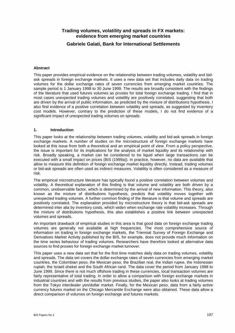
BIS Papers No 2 197
Trading volumes, volatility and spreads in FX markets:evidence from emerging market countries
Gabriele Galati, Bank for International Settlements
Abstract
This paper provides empirical evidence on the relationship between trading volumes, volatility and bid-ask spreads in foreign exchange markets. It uses a new data set that includes daily data on tradingvolumes for the dollar exchange rates of seven currencies from emerging market countries. Thesample period is 1 January 1998 to 30 June 1999. The results are broadly consistent with the findingsof the literature that used futures volumes as proxies for total foreign exchange trading. I find that inmost cases unexpected trading volumes and volatility are positively correlated, suggesting that bothare driven by the arrival of public information, as predicted by the mixture of distributions hypothesis. Ialso find evidence of a positive correlation between volatility and spreads, as suggested by inventorycost models. However, contrary to the prediction of these models, I do not find evidence of asignificant impact of unexpected trading volumes on spreads.
1. Introduction
This paper looks at the relationship between trading volumes, volatility and bid-ask spreads in foreignexchange markets. A number of studies on the microstructure of foreign exchange markets havelooked at this issue from both a theoretical and an empirical point of view. From a policy perspective,the issue is important for its implications for the analysis of market liquidity and its relationship withrisk. Broadly speaking, a market can be considered to be liquid when large transactions can beexecuted with a small impact on prices (BIS (1999a)). In practice, however, no data are available thatallow to measure this definition of foreign exchange market liquidity directly. Instead, trading volumesor bid-ask spreads are often used as indirect measures. Volatility is often considered as a measure ofrisk.
The empirical microstructure literature has typically found a positive correlation between volumes andvolatility. A theoretical explanation of this finding is that volume and volatility are both driven by acommon, unobservable factor, which is determined by the arrival of new information. This theory, alsoknown as the mixture of distributions hypothesis, predicts that volatility moves together withunexpected trading volumes. A further common finding of the literature is that volume and spreads arepositively correlated. The explanation provided by microstructure theory is that bid-ask spreads aredetermined inter alia by inventory costs, which widen when exchange rate volatility increases. Throughthe mixture of distributions hypothesis, this also establishes a positive link between unexpectedvolumes and spreads.
An important drawback of empirical studies in this area is that good data on foreign exchange tradingvolumes are generally not available at high frequencies. The most comprehensive source ofinformation on trading in foreign exchange markets, the Triennial Survey of Foreign Exchange andDerivatives Market Activity published by the BIS, for example, does not provide much information onthe time series behaviour of trading volumes. Researchers have therefore looked at alternative datasources to find proxies for foreign exchange market turnover.
This paper uses a new data set that for the first time matches daily data on trading volumes, volatilityand spreads. The data set covers the dollar exchange rates of seven currencies from emerging marketcountries, the Colombian peso, the Mexican peso, the Brazilian real, the Indian rupee, the Indonesianrupiah, the Israeli shekel and the South African rand. The data cover the period from January 1998 toJune 1999. Since there is not much offshore trading in these currencies, local transaction volumes arefairly representative of total trading. In order to allow a comparison with foreign exchange markets inindustrial countries and with the results from previous studies, the paper also looks at trading volumesfrom the Tokyo interdealer yen/dollar market. Finally, for the Mexican peso, data from a fairly activecurrency futures market on the Chicago Mercantile Exchange were also obtained. These data allow adirect comparison of volumes on foreign exchange and futures markets.

198 BIS Papers No 2
A main finding using this data set is that in most cases unexpected trading volume and volatility arepositively correlated, suggesting that they both react to the arrival of new information, as the mixture ofdistributions hypothesis predicts. This result is in line with the findings of the literature that relies onfutures data. The markets for the Mexican peso and the real, however, provide important exceptions.In these two cases, the relationship between unexpected volumes and volatility is not statisticallysignificant. I also find evidence of a positive correlation between volatility and spreads, as suggestedby inventory cost models. However, the results do not show a significant impact of trading volumes onspreads.
The remainder of the paper is organised as follows. Section 2 reviews the main contributions to theliterature on the relationship between trading volumes, volatility and spreads. Section 3 describes thedata set that is used. In Section 4, I present some descriptive evidence on the relationship betweenvolumes, volatility and spreads. I then use regression analysis to test whether the mixture ofdistribution hypothesis holds in foreign exchange markets. Section 5 concludes.
2. Literature review
There is an extensive literature on the relationship between trading volumes and volatility in financialmarkets. Karpoff (1987) provides a good overview of the early literature. Most of the research hasfocused on stock markets and futures markets, for which data on volumes are more easily available.An important finding is that trading volume and price variability are positively correlated at differentfrequencies. The coefficient is highest for contemporaneous correlations. However, it does not alwaysappear to be very sizeable. Evidence was found by Harris (1986) and Richardson et al. (1987) forstock markets and by Cornell (1981) for commodity futures.
The empirical work on foreign exchange markets has suffered from the problem that good data ontrading volumes are not easily available for foreign exchange markets, since unlike equity markets,they are for a large part decentralised. Different data sources were used to describe the time seriesbehaviour of trading volumes.1 Many studies used data on futures contracts, which can be easilyobtained, to proxy for interbank trading volumes. Studies that have found a positive correlationbetween volumes and volatility in these markets include Grammatikos and Saunders (1986), Battenand Bhar (1993) and Jorion (1996). An obvious drawback of these data sets is that trading in futures isvery small compared to OTC volumes (Dumas (1996)). In the first quarter of 1998, for example, totalturnover of currency futures traded on organised exchanges amounted to roughly $70 billion (BIS(1998)), compared to total OTC turnover in spot, forward and swap markets of about $1500 billion (BIS(1999b). While these two markets may still be closely linked through arbitrage (Lyons (2000)), littleevidence is available on this link.
A widely used source of information on foreign exchange trading, the Triennial Survey of ForeignExchange and Derivatives Market Activity published by the BIS, provides extensive cross-sectionalinformation but very little information on the time series behaviour of turnover. Hartmann (1998b)makes efficient use of these data by combining a large cross-section of exchange rates taken from theBIS Triennial Survey with two time series observation into a panel but still faces the problem of havinglimited time series information.
A number of papers analysed data on indicative quotes provided by Reuters through its FXFX page.2
However, these quotes do not represent actual trades and it is not possible to infer from a quote forwhich volume it is given. Spreads that are quoted on the Reuters screen are generally far from actual,traded spreads.3 Moreover, it is common for banks that act as data providers to program anautomated data input, e.g. by having a particular quote entered at regular time intervals. This isespecially true for smaller banks that may have an interest in quoting prices in order to advertise theirpresence in a particular market segment. Finally, when an important event occurs, traders are likely toact and trade rather than entering data for Reuters. Hence, Reuters tick frequency may be low at times
1 A good overview of the characteristics of data sets used in the literature can be found in Lyons (2000).
2 See, eg Goodhart and Figliuoli (1991), Bollerslev and Domowitz (1993). And Melvin and Yi (2000).
3See also Hartmann (1998a) , p.142.

BIS Papers No 2 199
of high trading activity and high when markets are calm. The relationship between quote frequencyand actual trading activity is therefore likely to be quite noisy.
An alternative source of information is the Bank of Japan’s data set on brokered transactions in theTokyo yen/dollar market, which has been used by Wei (1994) and Hartmann (1999). Again, a problemwith these data is that they represent only a fraction (about one-sixth) of total turnover in the Tokyoyen/dollar market and not more than 5% of the global yen/dollar market.
A fruitful approach has been to look at high-frequency data on actual transactions in the OTC market.One such data set, used by Lyons (1995), covers all transactions that a foreign exchange dealer inNew York entered with other dealers in one week in 1992. Goodhart, Ito and Payne (1996) analysedata on electronically brokered interdealer transactions that occurred on one day in 1993. While thesedata provide a wealth of information, including information on the direction of order flows, theynecessarily cover only a limited segment of foreign exchange markets and span a relatively short timeperiod.
Different theoretical explanations have been offered for the co-movement of trading volumes andvolatility. Early work was based on models of “sequential information arrival” (Copeland (1976,1977)),according to which information reaches one market participant at a time. As that agent reacts to thearrival of news, his demand curve will shift, thereby leading to a positive correlation between volumeand volatility. An alternative explanation of the volume-volatility correlation is based on the “mixture ofdistribution hypothesis” first proposed by Clark (1973). According to this hypothesis, volume andvolatility are both driven by a common, unobservable factor. This factor reflects the arrival of newpublic information, and determines a positive correlation between unexpected turnover andunexpected volatility. Tauchen and Pitts (1983) show that volume and volatility can co-move for tworeasons. First, as the number of traders grows, market prices become less volatile. Second, given thenumber of traders, an increase in volume reflects a higher disagreement among traders and henceleads to higher volatility. This link is stronger when new information arrives at a higher rate.
A number of studies looked at the relationship between volumes and volatility by testing the commonobservation that in both bond and equity markets, an upward movement of the market is generallyassociated with higher transaction volumes. The empirical evidence for this relationship is weak. Whilesome studies (e.g. Epps (1975, 1977), Rogalski (1978) and Richardson et al. (1987)) have foundweakly supportive evidence, other studies (e.g. James and Edminster (1983) and Wood et al. (1985))have failed to detect any significant correlation. Moreover, no favourable evidence has been found forfutures markets.
Models that explain bid-ask spreads in terms of inventory costs establish a link between bid-askspreads, volatility and trading volumes. One determinant of inventory costs is the cost of maintainingopen positions, which is positively related to price risk.4 According to this view, exchange rate volatilityincreases price risk and thereby pushes up spreads. Supportive evidence is provided byBessembinder (1994), Bollerslev and Melvin (1994) and Hartmann (1999), who found a positivecorrelation between spreads and expected volatility measured by GARCH forecasts.
A second determinant of inventory costs is trading activity. Trading volumes can have a differentimpact on spreads depending on whether they are expected or unexpected. Expected trading volumesshould be negatively correlated with spreads to the extent that they reflect economies of scale and areassociated with higher competition among market makers (Cornell (1978)). By contrast, unexpectedtrading volumes should have a positive impact on spreads to the extent that they are associated withhigher volatility through the mixture of distribution hypothesis.
4The microstructure literature analyses two other types of costs, order processing costs (i.e. costs of providing liquidityservices) and asymmetric-information costs (Bessembinder (1994), Jorion (1996) Hartmann (1999), Lyons (2000)). Whileorder processing costs are arguably small in foreign exchange market (Jorion (1996)), there is no consensus on theimportance of asymmetric-information costs.

200 BIS Papers No 2
3. The data
Exchange rates
This paper looks at the dollar exchange rates of seven currencies from emerging market countries: theIndonesian rupiah, the Indian rupee, the Mexican peso, the Brazilian real, the Colombian peso, theSouth African rand and the Israeli shekel.5 The sample period is January 1998 to June 1999.6
According to the IMF classification, during this period these exchange rates either floatedindependently or were managed in some form (Table 1). Figure 1 and Table 2 provide information ontheir behaviour. As a benchmark for comparison, information on the yen/dollar rate is also shown.Overall, all seven emerging market currencies depreciated against the dollar. The depreciation wasparticularly sharp following the Russian crisis in August 1998, except in the case of the real.
The real depreciated at a constant rate against the dollar in 1998. Following intense speculativepressures, Brazilian authorities had to float it freely on 15 January 1999 and it plunged from 1.1 toalmost 2.2 real/dollar. The real recovered somewhat in the following months, and in June 1998 tradedaround a level of 1.75 to the dollar. The Mexican peso depreciated through most of 1998 and early1999. However, it moved within a much smaller range than the real. The Mexican peso’s weaknesswas exacerbated following the Russian crisis in August 1998, when it depreciated by around 20%against the dollar. It also fell, albeit not as much, in January 1999, during the period of speculativeattacks on the real. The Colombian peso’s downward trend and fluctuation range against the US dollarwere similar to those of the Mexican peso. In August 1998, pressure on the peso stepped up, inducingthe authorities to widen the intervention band by 9%, effectively devaluing the currency. The pesocame under renewed pressure in March 1999 and June 1999, when it devalued by about 20%.
The Indian rupee’s behaviour was characterised by periods of stability followed by sharp downwardmovements. The Indonesian rupiah fell sharply in January and in July 1998. Its volatility declined in1999 but remained still very high.
The South African rand depreciated markedly against the dollar around the time of the Russian crisisin the summer of 1998. In the following months it recouped part of its losses but in 1999 trended downagain. In 1998, the shekel followed a slightly depreciating trend against the dollar. It fell by 20% afterthe Russian crisis but stabilised in the following weeks.
Figure 3 and Table 3 report information on the percentage exchange rate changes for the sevencurrencies. For the real, statistics are presented also separately for the period January-June 1999,during which it floated. Between January 1998 and June 1999, the average daily percentage changeof most of the currencies was significantly positive, with the exceptions of the Colombian peso and therupee. Their standard deviation ranged between 0.29 for the rupee and 4.24 for the rupiah. Over thesame period, the standard deviation of the yen/dollar rate was close to 1. Most exchange rate changesexhibited positive skewness, consistently with their downward trend, and leptokurtosis. Table 4suggests that the exchange rate changes exhibited very little persistence.
Volatility
Figure 3 shows the historical volatility of the seven exchange rates computed over moving windows ofone month. Summary statistics are reported in Table 5. In terms of their volatility, the seven exchangerates can be divided into two groups. The real and the rupiah experienced sharp volatility spikes andwere characterised by very high average volatility. By contrast, the historical volatilities of the rupee,the shekel and the Colombian peso remained quite low, averaging less than 8%. The rand’s volatilitywas relatively low on average, but it spiked at about 50%.
Table 5 shows that the volatility of the yen/dollar exchange rate during the same period averaged15%. This is much less than the volatility of the exchange rate of the real or the rupiah vis-à-vis thedollar, but more than the volatility of the other five exchange rates in this data set.
5 See, eg Goodhart and Figliuoli (1991), Bollerslev and Domowitz (1993). And Melvin and Yi (2000).
6The choice of the sample period is dictated by the availability of data on trading volumes.
BIS Papers No 2 201
A finding that is common for exchange rates and other asset prices is the existence of volatilityclustering, i.e. the fact that periods of persistent turbulence are followed by periods of relative calm. Inthe finance literature, this phenomenon has typically been described by some ARCH-type models.Tests for ARCH-type effects presented in Table 6 suggest that the exchange rates under investigation- possibly with the exception of the Colombian peso - exhibit some ARCH-type behaviour. Thisbehaviour seems to be fairly well captured by a GARCH (1,1) model.
Finally, Table 7 present evidence that for half of the exchange rates, volatility follows a time trend. Thetrend is positive for the Colombian peso and the real and negative for the rupee and rupiah. There isno evidence of weekend effects.
Trading volumes
A large literature has documented the behaviour of trading volumes in stock markets and bondmarkets. By contrast, there is relatively little work on foreign exchange markets because of thedifficulty of obtaining data with a sufficiently high frequency in this decentralised market. In this paper Iuse daily data on local turnover on seven exchange rates from emerging market countries. Thesample period is January 1998 to June 1999, except for the rupiah, for which data are available onlyfrom 1 January to 30 June 1999. Since there is not much offshore trading in these currencies, localtransaction volumes are fairly representative of total trading.7 As a benchmark, I also included tradingvolumes from the Tokyo interbank market, which were used in previous studies. The time series of thetrading volumes are shown in Figure 1 and summary statistics are reported in Table 8.
A comparison with data from the 1998 Triennial Survey suggests that taken together, trading in theseven currency pairs accounts for roughly 1-2% of total foreign exchange market turnover. Theindividual markets are characterised by very different levels of activity. The most active markets werethose for the Mexican peso, the real and the rand. To get an idea of the size of these markets, tradingof dollars against one of these currencies averaged about one-third of local trading of Canadian orAustralian dollars against the US dollar in April 1998. Taking the yen/dollar market as a benchmark,the size of these markets is slightly smaller than the interbank market in Tokyo. The market for therupee also appeared to be quite active ($3.5 billion a day), much more than the market for theIndonesian rupiah ($1 billion per day), which in 1995 and 1996 was the most active foreign exchangemarket in emerging market countries with an average daily turnover of more than $8 billion (BIS(1997)). Transaction volumes for the Colombian peso and the shekel instead are relatively small.
Figure 1 reveals some interesting facts about the behaviour of trading volumes. First, it shows alsothat the foreign exchange turnover involving the real, the Colombian and the Mexican peso and therand fell substantially around the end of August 1998, at time when the Russian crisis sparked a globalreduction of liquidity in financial markets. The decline in trading volumes was particularly sharp inMexico and Brazil.
Second, while trading volumes behaved differently around periods of speculative pressures, theyalways fell substantially once the pressures abated.8 This fact can be illustrated with the examples ofthe real and the Colombian peso. At the time of the speculative attack on the real in January 1999,trading volumes for the real rose for a short time and became more volatile. After Brazilian authoritiesdecided to float the real on 12 January 1999, trading of reais against dollars remained very volatile forseveral weeks and before shrinking substantially around mid-February. In the following months,turnover built up again steadily but remained below levels observed before the crisis.
The Colombian peso was subject to two rounds of pressure in 1999. When pressure mounted first inMarch, there appears not to have been a significant increase in foreign exchange turnover. Followingthis period, daily turnover dried up from about $200 mn to less than $50 mn. At the time of the secondattack on the peso in June 1999, turnover increased sharply to $150 mn or more. Since our sampleperiod ends on 30 June 1999, it is not possible to verify how trading volumes behaved after thesecond attack.
7Until 1997 there was a quite active rupiah/dollar market in Singapore. However, most of this activity disappeared followingthe Asian crisis.
8This is true even when volumes are measured at constant exchange rates.

202 BIS Papers No 2
Regressions of trading volumes on a constant, a linear time trend and a dummy variable capturingweekend effects show a negative trend for trading in the Colombian and Mexican peso, the real (untilJanuary 1999) and the rand. By contrast, there is evidence that turnover of the rupiah followed apositive time trend. The volume of yen/dollar transactions brokered in Tokyo instead did not exhibitany time trend. Graph 2, which plots turnover in selected emerging markets over a longer horizon (andat a lower frequency), puts these findings in perspective. It suggests that trading in emerging marketcurrencies rose in the mid-1990s but in most cases fell after the Asian crisis and again at the time ofthe global reduction of liquidity in financial markets in 1998. Finally, Table 7 shows also that weekendeffects appear to be present in about half of the cases.
For the Colombian peso, data on the transaction frequency is also available. It is sometimes arguedthat the combination of these data and trading volumes provides a good indicator on market liquidity.Table 8 suggest that for the Colombian peso/dollar exchange rate the behaviour and the statisticalproperties of turnover and transaction frequency are very similar.
Table 10 presents some summary statistics on the changes of daily trading volumes. On average,trading volumes for the Colombian peso, the rand, the real and the rupiah appear to be most stable.The statistic for the rupiah is particularly noteworthy and indicative of the low variability of turnoverassociated with the low activity after the Asian crisis. For the Colombian peso, the statistics forturnover and transaction frequency appear to be very similar. The Mexican peso and the shekel exhibitthe highest average variability of trading volumes.
Futures contracts for three exchange rates, the Mexican peso/dollar, the real/dollar and the rand/dollarrate are traded on the Chicago Mercantile Exchange.9 Table 9 provides summary statistics for theseseries. Trading is most active for the Mexican peso/dollar contracts, but in any case much less - nomore than 3% - than OTC turnover. Figure 3 shows that on many days there is actually no trading onthe exchanges at all involving the rand or the real. Exchange traded and OTC volumes appear not tohave co-moved closely in 1998 and 1999. The correlation coefficient of daily percentage changes isless than 1% for the Mexican peso, 4% for the rand and 18% for the real.
Spreads
Table 12 reports summary statistics on bid-ask spreads, expressed as a fraction of the exchange rate.As a benchmark for comparison, it also provides information on the spreads on brokered yen/dollartransactions in Tokyo. A caveat about these data is that they refer to indicative quotes rather than toactual transactions. Spreads on actual trades may be much smaller (and possibly less volatile),especially when one looks at electronically brokered transactions. 10 Subject to these caveats,Table 12 shows that spreads on exchange rates from emerging market countries are much higher andmuch more volatile than spreads on the yen/dollar exchange rate. Their average in 1998 and 1999ranged from 0.12% of the exchange rate for the Mexican peso to more than 2% for the rupiah,compared to spreads around 0.05% for the yen/dollar market. Table 7 provides some additionalinformation on the variations of the bid-ask spreads.
4. Volumes, volatility and spreads
Trading volumes and volatility
A well-established fact for stock markets is that trading volumes are positively correlated with pricevariability.11 A similar result has also been found for foreign currency futures (Grammatikos andSaunders (1986)). The middle panels in Graph 2 suggest that when turmoil hits foreign exchangemarkets, both volatility and trading volumes increase. Once the currency has depreciated markedly,trading volumes tend to fall substantially.
9There is also active trading in real/dollar futures contracts on the BM&F in São Paolo and on the rand in London.
10See Lyons (1995) and Hartmann (1999) and Cheung and Chinn (1999). Most of yen/dollar spot transactions between banksare nowadays conducted through electronic brokers and have spreads about two to three hundredths of a US cent.
11See Karpoff (1987, pp.112-3) for an overview of this literature.

BIS Papers No 2 203
In terms of the contemporaneous correlation between daily foreign exchange turnover and exchangerate volatility, Table 14 shows positive coefficients for five out of seven emerging market exchangerates (the dollar exchange rates of the Colombian peso, rand, rupee, rupiah and shekel). Thecorrelation is also positive for the yen/dollar rate traded in the Tokyo interbank market. This holdsirrespectively of whether exchange rate volatility is measured by absolute values of percentagechanges, squared returns or the standard deviation of daily returns computed over rolling windows ofone-month. By contrast, I find a negative correlation for the real and the Mexican peso.
Regressions of volatility on a constant, a time trend, a day-of-the-week dummy and trading volumesgives positive and statistically significant coefficients in all cases except the real and the Mexican peso(Table 16). For the Colombian peso, a regression of volatility on the number of deals per day alsogives a positive and statistically significant coefficient. With the exception of the real and the Mexicanpeso, these results are consistent with the finding of a positive correlation of volatility and volumefound for currency futures (Grammatikos and Saunders (1986), Jorion (1996)). Table 15 shows that forthe Mexican peso, exchange traded data give a positive correlation between volatility and volumes.This result suggests that exchange traded data may not always be an appropriate proxy for totalinterbank trading.
Another interesting issue is whether trading volumes are “directional” in the sense that they increase(decrease) when asset prices increase (decrease). Testing this hypothesis involves testing for apositive correlation of volumes and price changes. There is some, albeit weak, evidence in favour ofthis hypothesis for stock and bond markets (Karpoff (1987)). By contrast, there is no supportingevidence for futures markets. Table 14 does not provide clear evidence of a positive relationshipbetween volumes and price changes in foreign exchange markets. For some exchange rates - theColombian and the Mexican peso, rand, rupee and shekel - changes are positively correlated withtrading volumes but the correlation coefficients are small. The correlation coefficient is negative for thereal and rupiah. The same is true for yen/dollar rate traded in Tokyo.
A related question is whether trading volume and exchange rate changes are related in an asymmetricfashion, i.e. whether volumes are higher when a currency appreciates or when it depreciates againstthe dollar. Karpoff (1987) argued that most empirical findings for stock markets support what he callsan “asymmetric volume-price change hypothesis”, i.e. a fundamentally different relationship betweenvolume and price changes for positive and negative price changes. The evidence presented inTable 14 appears only weakly consistent with this hypothesis. For the Mexican peso, rupee, shekeland the yen, the relationship between volumes and exchange rate changes is almost identical in thetwo cases. For the other currencies, volumes change more in the case of a depreciation than in thecase of an appreciation.
The positive correlation between volumes and volatility found for most of the exchange rates is unlikelyto be a reflection of changes in the number of traders active in these markets. These changes appearrather to have occurred in the mid-1990s, when banks increasingly moved into emerging markets, andafter the Asian crisis, when the sharp fall in turnover was accompanied by a significant decline in thenumber of traders. A more plausible explanation for the positive correlation between turnover andvolatility is that both variables are driven by a common, unobservable factor. According to the mixtureof distribution hypothesis, this factor reflects the arrival of new information, and determines a positivecorrelation between unexpected turnover and unexpected volatility. Moreover, as Tauchen and Pitts(1983) show, volume and volatility can co-move because, given the number of traders, an increase involume may reflect a higher disagreement among traders, which also leads to higher volatility. Theco-movement is closer when new information arrives at a higher rate.
To test this hypothesis, I split volatility and trading volumes into expected and unexpectedcomponents. I use estimates from a GARCH(1,1) model to describe expected volatility. This modelappears to fit the time series well.12 Ideally, volatility implied in option prices could be used, since thereis evidence that it outperforms GARCH models in providing forecasts of future volatility.13 However,option contracts for currencies of emerging market countries are not very liquid, particularly after theAsian crisis. The GARCH(1,1) model can be written as:
12Following a common practice of the literature, the GARCH-model is fitted on the entire time series, therefore yielding in-sample forecasts.
13Jorion (1996); Galati and Tsatsaronis (1996).
204 BIS Papers No 2
where Rt is the return, its mean and ht its conditional variance at time t.
In order to measure expected trading volumes, I used the Box-Jenkins analysis to select aparsimonious time series representation for the volume series, which are taken in logs. Time seriesmodels were fitted on the levels of trading volumes since Augmented Dickey-Fuller test suggest thatthey are stationary. AR models, in most cases of first order, seemed appropriate to represent theturnover series. These models allow to split trading volumes into an expected and an unexpectedcomponent.
The regression equation that is estimated takes the following form:
where total volatility R2t+1 is defined as squared returns, expected volatility ht+1 is the one-step-ahead
conditional return variance from a GARCH(1,1) specification, and log-volumes are decomposed intoan expected component Et(v) and an unexpected component [vt+1-Et(v)] by using a fitted AR seriesand its residuals. A linear time trend and a dummy capturing weekend effects are also included.
Table 17 reports the regression results. The coefficient on unexpected turnover is positive andstatistically significant at 1% or 5% in all the regressions for exchange rates from emerging marketcountries, except those for the Mexican peso and the real. For these two currencies, the coefficientsare negative but not statistically significant. A positive, significant coefficient is also found for theyen/dollar rate traded in Tokyo. Except for the Mexican peso and the real, the results support the ideathat information flow drives volatility and volumes, as implied by the mixture of distributions hypothesis.This result is consistent with the conclusion of the literature that used data on currency futures (Jorion(1996)). These results are independent of market size: they hold for both for the smallest market(Colombian peso/dollar) as for the biggest market (ran/dollar) in emerging market countries, as well asfor the even bigger yen/dollar interbank market in Tokyo. This is consistent with the finding presentedin Batten and Bhar (1993) for futures markets. Differently from Jorion’s results, however, expectedvolumes also have a positive, significant effect on volatility in three cases (rupee, shekel and yen).
Table 18 shows the results for regressions that also include expected volatility, measured by theGARCH forecast, among the explanatory variables. The coefficient on unexpected turnover remainspositive and statistically significant in most cases. This is in line with the results presented in Jorion(1996). Again, the coefficient on unexpected trading volume it is negative but not statisticallysignificant for the Mexican peso and the real. In these cases only, the GARCH volatility forecast is alsosignificant.
Overall, the results support the idea that the arrival of new public information drives the positivecorrelation between volumes and volatility, as postulated by the mixture of distribution hypothesis.Favourable evidence is found for four out of six exchange rates from emerging market countries andfor the Tokyo interbank yen/dollar market. These findings appear to be independent of market size. Bycontrast, the mixture of distribution hypothesis appears not to hold for the Mexican peso/dollar andreal/dollar markets.
Trading volumes and bid-ask spreads
Figure 2 highlights that in foreign exchange markets in emerging market countries, bid-ask spreadsspiked during times in which volatility sharply increased and turnover fell. While spreads tended tonarrow shortly after these episodes, in some cases they remained wide for some time. Table 14 showsthat in foreign exchange market in emerging market countries, spreads and volatility are positivelycorrelated. In most cases spreads and trading volumes are negatively correlated, a result thatcontrasts with findings of the early literature.14 By contrast, the behaviour of spreads appears totallyunrelated to changes in volumes and volatility in the Tokyo yen/dollar interbank market, as indicatedby correlation coefficients close to zero.
14See eg Glassman (1987).
12
110),,0(~,)1( −− ++=+= tttttt hrhhNrrR βααµ
154132112
1 )]([)()2( ++++ +++−+++= tttttt wtvEvvEhR εβββββα

BIS Papers No 2 205
Models that explain bid-ask spreads in terms of inventory costs establish a link between bid-askspreads, volatility and trading volumes. One determinant of inventory costs is the cost of maintainingopen positions, which is positively related to price risk (Jorion (1996)). According to this view,exchange rate volatility increases price risk and thereby pushes up spreads. Supportive evidence isprovided by Bessembinder (1994), Bollerslev and Melvin (1994) and Hartmann (1999), who found apositive correlation between spreads and expected volatility measured by GARCH forecasts.
A second determinant of inventory costs is trading activity. Trading volumes can have a differentimpact on spreads depending on whether they are expected or unexpected. Expected trading volumesshould be negatively correlated with spreads if they reflect economies of scale and are associated withhigher competition among market makers (Cornell (1978)). By contrast, unexpected trading volumesshould have a positive impact on spreads to the extent that they are associated with higher volatilitythrough the mixture of distribution hypothesis.15
To test these assertions, I regressed bid-ask spreads on the GARCH variance forecasts andmeasures of expected and unexpected trading volumes:
The results are presented in Table 19. Consistently with the findings of the literature, the coefficient onthe GARCH variance forecast is positive and statistically significant, suggesting that volatilityinfluences bid-ask spreads through its effect on inventory costs. However, in contrast to thepredictions of the theory, I do not find positive and significant coefficients on unexpected volumes. Thecoefficients on expected volumes are also not statistically significant. This latter result is not surprising,since the sample period is likely to be too short to allow for changes in these foreign exchangemarkets that lead to more efficient trade processing and higher competition among market makers.
5. Conclusions
This paper tried to provide a contribution to the literature on the microstructure of foreign exchangemarkets by investigating the empirical relationship between trading volumes, volatility and bid-askspreads. Until now most of the research in this area has relied on data on futures markets, since gooddata on turnover in foreign exchange markets were not easily available. One important critique of thisapproach is that volumes in futures markets are not representative of total foreign exchange marketactivity. This paper uses a new data set that includes daily data on trading volumes for the dollarexchange rates of seven currencies from emerging market countries, the Indonesian rupiah, the Indianrupee, the Mexican peso, the Brazilian real, the Colombian peso, the South African rand and theIsraeli shekel. To allow a comparison with other studies, it also looks at trading volumes from theTokyo interdealer yen/dollar market. The data set covers the sample period from 1 January 1998 to30 June 1999.
An important result is that unexpected trading volumes and volatility are positively correlated,suggesting that they both respond to the arrival of new information, as the mixture of distributionshypothesis predicts. This is consistent with the findings of the literature that relies on futures data. Itsuggests that the observation that futures markets are not representative is not “damaging” (Dumas(1996)). The markets for the Mexican peso and the real, however, provide important exceptions. Inthese two cases, the relationship between unexpected volumes and volatility is negative but notstatistically significant. Moreover, for the Mexican peso data from foreign exchange market and fromfutures market give opposite results, as unexpected futures volumes and volatility are positivelycorrelated.
I also find evidence of a positive correlation between volatility and spreads, as suggested by inventorycost models. This result is also consistent with the findings of the literature. However, in contrast toprevious studies I do not find evidence of a significant impact of unexpected trading volumes onspreads.
15See Jorion (1996).
ttvttttt wEvvEhS εββββα ++−+++= −−+ 4)(131211 ][)()3(

206 BIS Papers No 2
References
Batten and Bhar (1993) “Volume and volatility in yen futures markets: Within and across three differentexchanges”, Macquarie University Working Paper.
Galati, G and K Tsatsaronis (1996) “The Information Content of Implied Volatility from CurrencyOptions”, BIS.
Hendrik Bessembinder (1994) “Bid-Ask Spreads in the Interbank Foreign Exchange Markets”, JournalFinancial Economics, 35(3), 317-348.
BIS (1997) 67th Annual Report.
BIS (1998) International Banking and Financial Market Developments, November.
BIS (1999a) “Market Liquidity: Research Findings and Selected Policy Implications”, Report for theCGFS.
BIS (1999b) Triennial Survey of Foreign Exchange and Derivatives Market Activity.
Bollerslev, T and I Domowitz (1993) “Trading patterns and prices in the interbank foreign exchangemarket”, Journal of Finance, 48, 1421-43.
Bollerslev, T and Michael Melvin (1994) “Bid-ask spreads and volatility in the foreign exchange market:an empirical analysis”, Journal of International Economics, 36, 355-372.
Yin-Wong Cheung and Menzie Chinn (1999) “Traders, market microstructure and exchange ratedynamics”, NBER Working Paper 7416, November.
Clark, P K (1973) “A subordinated stochastic process model with finite variance for speculative prices”,Econometrica, 41, 135-155.
Copeland (1976) “A model of asset trading under the assumption of sequential information arrival”,Journal of Finance, 31, 1149-1168.
Copeland (1977) “A probability model of asset trading”, Journal of Financial and Quantitative Analysis,12, 563-578.
Copeland and Galai (1983) “Information Effects on the Bid-Ask Spread”, Journal of Finance,31(December), 1457-1469.
Cornell, B (1978) “Determinants of the bid-ask spread on forward foreign exchange contracts underfloating exchange rates”, Journal of International Business Studies, 9, 33-41.
Cornell, B (1981) “The relationship between volume and price variability in futures markets”, TheJournal of Futures Markets, 1, 303-316.
Dumas, Bernard (1996) “Comment on Jorion”, in Frankel, Galli and Giovannini (1996) TheMicrostructure of Foreign Exchange Markets, University of Chicago Press, Chicago, 37-40.
Easley, David and Maureen O’Hara (1994) “Time and the Process of Security Adjustment”, Journal ofFinance, 47 (2), 577-605.
Epps, T W (1975) “Security price changes and transaction volumes: theory and evidence”, AmericanEconomic Review, 65, 586-597.
Epps, T W (1977) “Security price changes and transaction volumes: some additional evidence”,Journal of Financial and Quantitative Analysis, 12, 141-146.
Frankel, Jeffrey and Andrew Rose (1995) “Empirical Research on Nominal Exchange Rates”, inHandbook of International Economics, Vol.2, pp.1689-1721.
Frankel, Jeffrey Gianpaolo Galli and Alberto Giovannini (1996) The Microstructure of ForeignExchange Markets, University of Chicago Press, Chicago.
Glassman, Debra (1987) “Exchange Rate Risk and Transaction Costs: Evidence from Bid-AskSpreads”, Journal of International Money and Finance, 6(4), 479-490.
Goodhart, C and L Figliuoli (1991) “Every minute counts in financial markets”, Journal of InternationalMoney and Finance, 10, 23-52.
BIS Papers No 2 207
Goodhart, C, T Ito and R Payne (1996) “One day in June 1993: A study of the working of the Reuters2000-2 electronic foreign exchange trading system”, in Frankel, Galli and Giovannini (1996) TheMicrostructure of Foreign Exchange Markets, University of Chicago Press, Chicago, 107-179.
Grammatikos, T and A Saunders (1986) “Futures price variability: a test of maturity and volumeeffects”, Journal of Business, 59, 319-330.
Harris, L (1986) “Cross-security tests of the mixture of distributions hypothesis”, Journal of Financialand Quantitative Analysis, 21, 39-46.
Hartmann, Philipp (1998a) “Do Reuters spreads reflect currencies’ differences in global tradingactivity” in Currency composition and foreign exchange markets. Cambridge University Press, 132-162
Hartmann, Philipp (1998b) “Trading volumes and transaction costs: from the short run to the long run”in Currency composition and foreign exchange markets. Cambridge University Press.
Hartmann, Philipp (1999) “Trading Volumes and Transaction Costs in the Foreign Exchange Market”,Journal of Banking and Finance, 23, 801-824.
James, C and R O Edminster (1983) “The relation between common stock returns trading activity andmarket value”, Journal of Finance, 38, 1075-1086.
Jorion, Philippe (1996) “Risk and Turnover in the Foreign Exchange Market”, in Frankel, Galli andGiovannini (1996) The Microstructure of Foreign Exchange Markets, University of Chicago Press,Chicago, 19-36.
Karpoff, Jonathan (1987) “The Relation Between Price Changes and Trading Volume: A Survey”,Journal of Financial and Quantitative Analysis, 22(1), 109-126.
Lyons, Richard (1995) “Test of microstructural hypotheses in the foreign exchange market”, Journal ofFinancial Economics 39, 321-351.
Lyons, Richard (1996) “Foreign exchange volume: sound and fury signifying nothing?”, in Frankel,Galli and Giovannini (1996) The Microstructure of Foreign Exchange Markets, University of ChicagoPress, Chicago, 183-201.
Lyons, Richard (2000) The Microstructure Approach to Exchange Rates, MIT Press, forthcoming.
Richardson, G, S E Sefcik and R Thomson (1987) “A test of dividend irrelevance using volumereaction to a change in dividend policy"” Journal of Financial Economics, 17, 313-333.
Rogalski, R J (1978) “The dependence of prices and volume”, The Review of Economics andStatistics, 36, 268-274.
Shang-Jin Wei (1994) “Anticipations of foreign exchange volatility and bid-ask spreads”, NBERWorking Paper No.4737.
Tauchen, G and M Pitts (1983) “The price-variability volume relationship on speculative markets”,Econometrica, 51 (March), 485-505.
Wood, R A et al. (1985) “An investigation of transactions data for NYSE stocks”, Journal of Finance,60 (July), 723-739.

208 BIS Papers No 2
6. Tables and Graphs
Table 1
Exchange rate regimes, 1998–99
Currency Exchange rate regime
Colombian peso Managed floating within an intervention band
Mexican peso Independent float
Rand Independent float
Real Managed floating within an adjustable band against the US dollar (mid-1995 toJanuary 1999)
Rupee Independent float
Rupiah Free float (since the crisis in July 1997)
Shekel Managed with respect to a basket of currencies, with margins of fluctuations of +/– 15%.1
1 The shekel is fully convertible since May 1998.
Source: IMF Exchange Rate Arrangements and Restrictions, 1999.
Table 2
Summary statistics for the exchange rates levels
Mean Std. Dev. Min Max
Colombian peso 1486.19 116.28 1305.83 1752.18
Mexican peso 9.33 0.66 8.03 10.65
Rand 5.73 0.51 4.88 6.62
Real 1.36 0.3 1.12 2.19
Rupee 41.75 1.41 38.3 43.52
Rupiah 9614.66 2193.46 6000 16745
Shekel 3.89 0.24 3.55 4.37
Memo item:Yen/dollar 126.80 9.38 108.80 147.25
Notes: The sample period is 1 Jan. 1998 - 1 July 1999.
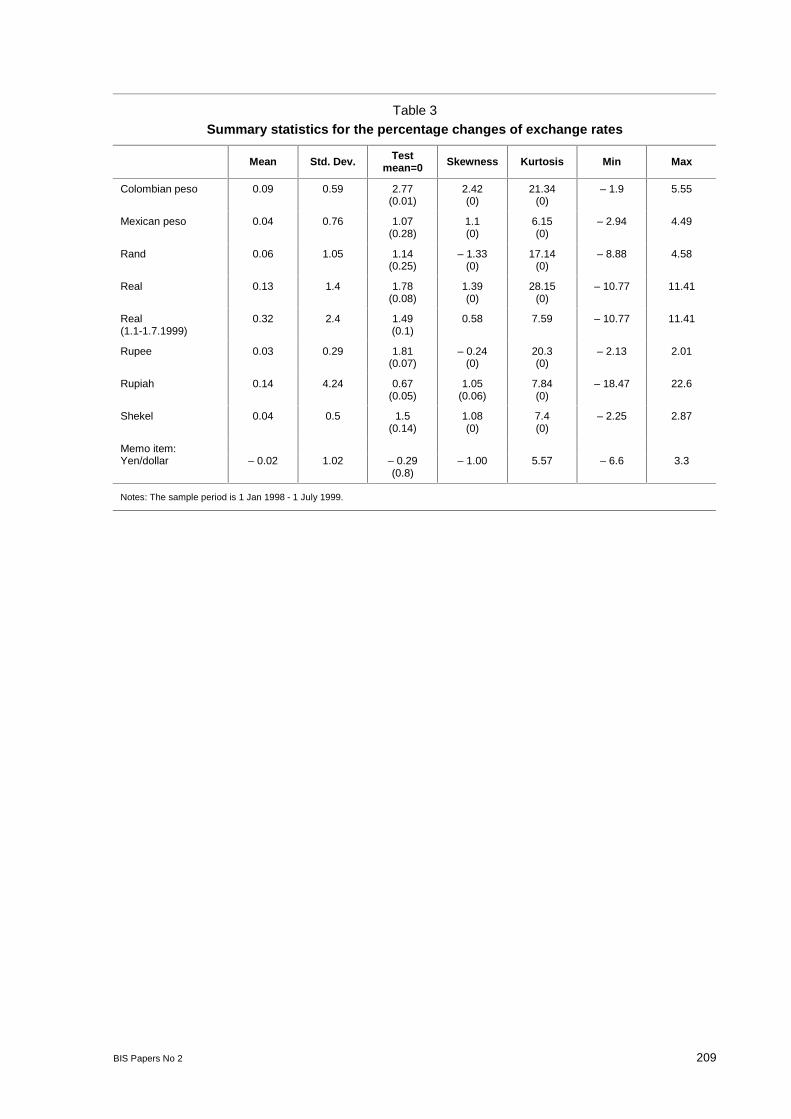
BIS Papers No 2 209
Table 3Summary statistics for the percentage changes of exchange rates
Mean Std. Dev. Testmean=0 Skewness Kurtosis Min Max
Colombian peso 0.09 0.59 2.77(0.01)
2.42(0)
21.34(0)
– 1.9 5.55
Mexican peso 0.04 0.76 1.07(0.28)
1.1(0)
6.15(0)
– 2.94 4.49
Rand 0.06 1.05 1.14(0.25)
– 1.33(0)
17.14(0)
– 8.88 4.58
Real 0.13 1.4 1.78(0.08)
1.39(0)
28.15(0)
– 10.77 11.41
Real(1.1-1.7.1999)
0.32 2.4 1.49(0.1)
0.58 7.59 – 10.77 11.41
Rupee 0.03 0.29 1.81(0.07)
– 0.24(0)
20.3(0)
– 2.13 2.01
Rupiah 0.14 4.24 0.67(0.05)
1.05(0.06)
7.84(0)
– 18.47 22.6
Shekel 0.04 0.5 1.5(0.14)
1.08(0)
7.4(0)
– 2.25 2.87
Memo item:Yen/dollar – 0.02 1.02 – 0.29
(0.8)– 1.00 5.57 – 6.6 3.3
Notes: The sample period is 1 Jan 1998 - 1 July 1999.
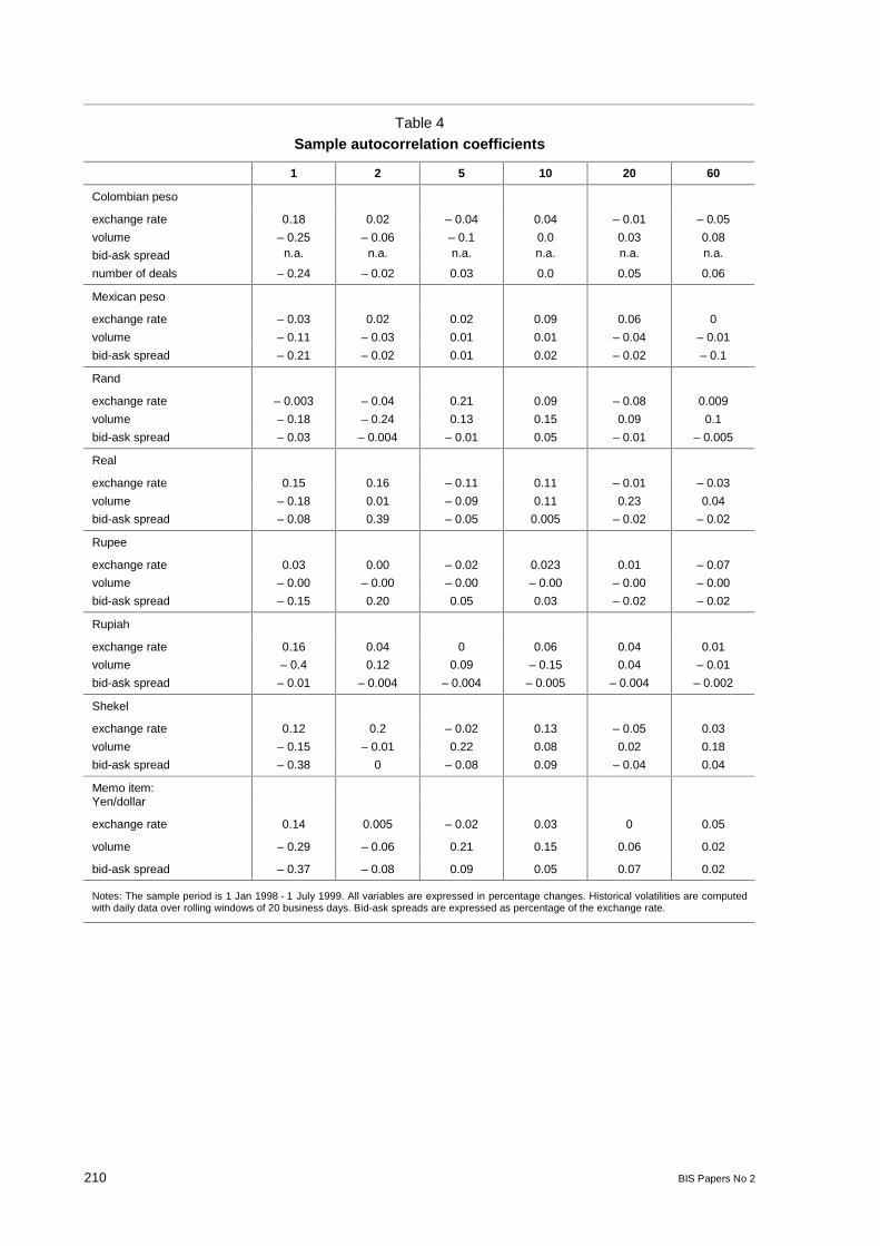
210 BIS Papers No 2
Table 4Sample autocorrelation coefficients
1 2 5 10 20 60
Colombian peso
exchange rate 0.18 0.02 – 0.04 0.04 – 0.01 – 0.05
volume – 0.25 – 0.06 – 0.1 0.0 0.03 0.08
bid-ask spread n.a. n.a. n.a. n.a. n.a. n.a.
number of deals – 0.24 – 0.02 0.03 0.0 0.05 0.06
Mexican peso
exchange rate – 0.03 0.02 0.02 0.09 0.06 0
volume – 0.11 – 0.03 0.01 0.01 – 0.04 – 0.01
bid-ask spread – 0.21 – 0.02 0.01 0.02 – 0.02 – 0.1
Rand
exchange rate – 0.003 – 0.04 0.21 0.09 – 0.08 0.009
volume – 0.18 – 0.24 0.13 0.15 0.09 0.1
bid-ask spread – 0.03 – 0.004 – 0.01 0.05 – 0.01 – 0.005
Real
exchange rate 0.15 0.16 – 0.11 0.11 – 0.01 – 0.03
volume – 0.18 0.01 – 0.09 0.11 0.23 0.04
bid-ask spread – 0.08 0.39 – 0.05 0.005 – 0.02 – 0.02
Rupee
exchange rate 0.03 0.00 – 0.02 0.023 0.01 – 0.07
volume – 0.00 – 0.00 – 0.00 – 0.00 – 0.00 – 0.00
bid-ask spread – 0.15 0.20 0.05 0.03 – 0.02 – 0.02
Rupiah
exchange rate 0.16 0.04 0 0.06 0.04 0.01
volume – 0.4 0.12 0.09 – 0.15 0.04 – 0.01
bid-ask spread – 0.01 – 0.004 – 0.004 – 0.005 – 0.004 – 0.002
Shekel
exchange rate 0.12 0.2 – 0.02 0.13 – 0.05 0.03
volume – 0.15 – 0.01 0.22 0.08 0.02 0.18
bid-ask spread – 0.38 0 – 0.08 0.09 – 0.04 0.04
Memo item:Yen/dollar
exchange rate 0.14 0.005 – 0.02 0.03 0 0.05
volume – 0.29 – 0.06 0.21 0.15 0.06 0.02
bid-ask spread – 0.37 – 0.08 0.09 0.05 0.07 0.02
Notes: The sample period is 1 Jan 1998 - 1 July 1999. All variables are expressed in percentage changes. Historical volatilities are computedwith daily data over rolling windows of 20 business days. Bid-ask spreads are expressed as percentage of the exchange rate.
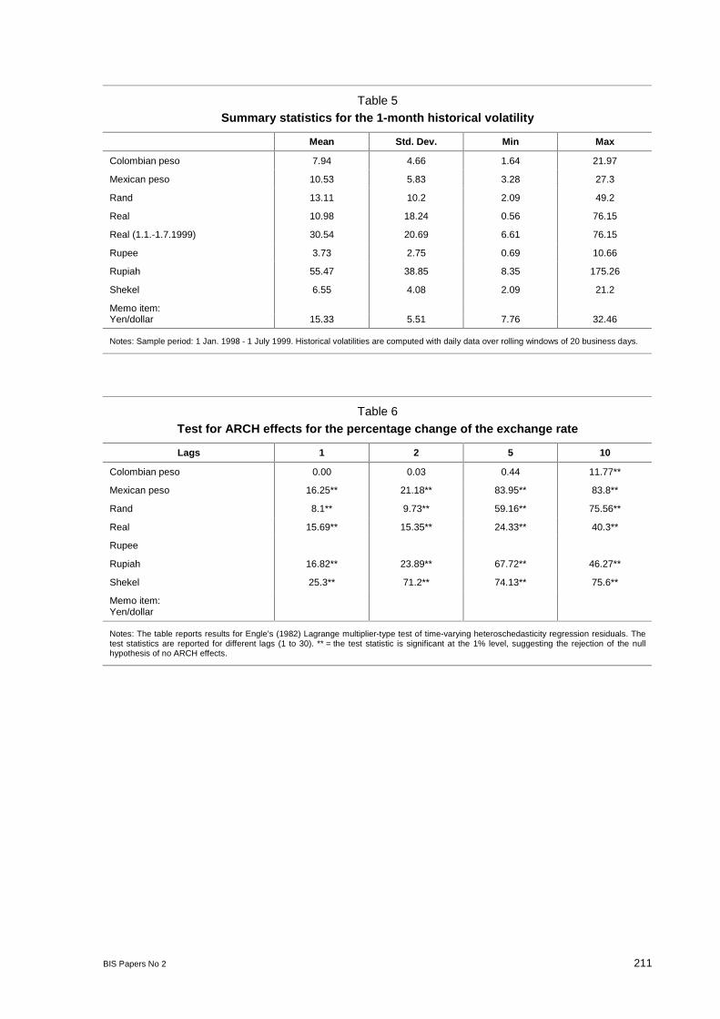
BIS Papers No 2 211
Table 5Summary statistics for the 1-month historical volatility
Mean Std. Dev. Min Max
Colombian peso 7.94 4.66 1.64 21.97
Mexican peso 10.53 5.83 3.28 27.3
Rand 13.11 10.2 2.09 49.2
Real 10.98 18.24 0.56 76.15
Real (1.1.-1.7.1999) 30.54 20.69 6.61 76.15
Rupee 3.73 2.75 0.69 10.66
Rupiah 55.47 38.85 8.35 175.26
Shekel 6.55 4.08 2.09 21.2
Memo item:Yen/dollar 15.33 5.51 7.76 32.46
Notes: Sample period: 1 Jan. 1998 - 1 July 1999. Historical volatilities are computed with daily data over rolling windows of 20 business days.
Table 6
Test for ARCH effects for the percentage change of the exchange rate
Lags 1 2 5 10
Colombian peso 0.00 0.03 0.44 11.77**
Mexican peso 16.25** 21.18** 83.95** 83.8**
Rand 8.1** 9.73** 59.16** 75.56**
Real 15.69** 15.35** 24.33** 40.3**
Rupee
Rupiah 16.82** 23.89** 67.72** 46.27**
Shekel 25.3** 71.2** 74.13** 75.6**
Memo item:Yen/dollar
Notes: The table reports results for Engle’s (1982) Lagrange multiplier-type test of time-varying heteroschedasticity regression residuals. Thetest statistics are reported for different lags (1 to 30). ** = the test statistic is significant at the 1% level, suggesting the rejection of the nullhypothesis of no ARCH effects.
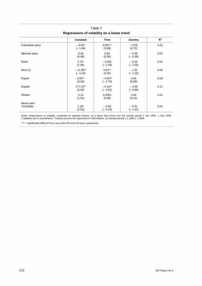
212 BIS Papers No 2
Table 7Regressions of volatility on a linear trend
Constant Time Dummy R2
Colombian peso – 0.63*(– 1.94)
0.001**(3.69)
– 0.09(0.72)
0.01
Mexican peso 0.45(0.98)
0.00(0.30)
– 0.06(– 0.39)
0.01
Rand 2.74*(1.94)
– 0.001(– 1.34)
– 0.54(– 1.55)
0.01
Real (1) – 11.95**(– 4.14)
0.01**(4.02)
– 1.02(– 1.19)
0.02
Rupee 0.60**(3.00)
– 0.00**(– 2.76)
0.06(0.89)
0.03
Rupiah 177.22**(4.94)
– 0.16**(– 4.81)
– 4.38(– 0.86)
0.11
Shekel 0.13(1.01)
0.0001(0.90)
0.03(0.41)
0.01
Memo item:Yen/dollar 1.18*
(1.93)– 0.00
(– 0.15)– 0.31
(– 1.42)0.01
Notes: Regressions of volatility, computed as squared returns, on a linear time trend over the sample period 1 Jan 1998 - 1 July 1999.T-statistics are in parentheses. Trading volumes are expressed in US$ millions. (1) Sample period 1.1.1999-1.7.1999.
*,** = significantly different from zero at the 5% and 1% level, respectively.
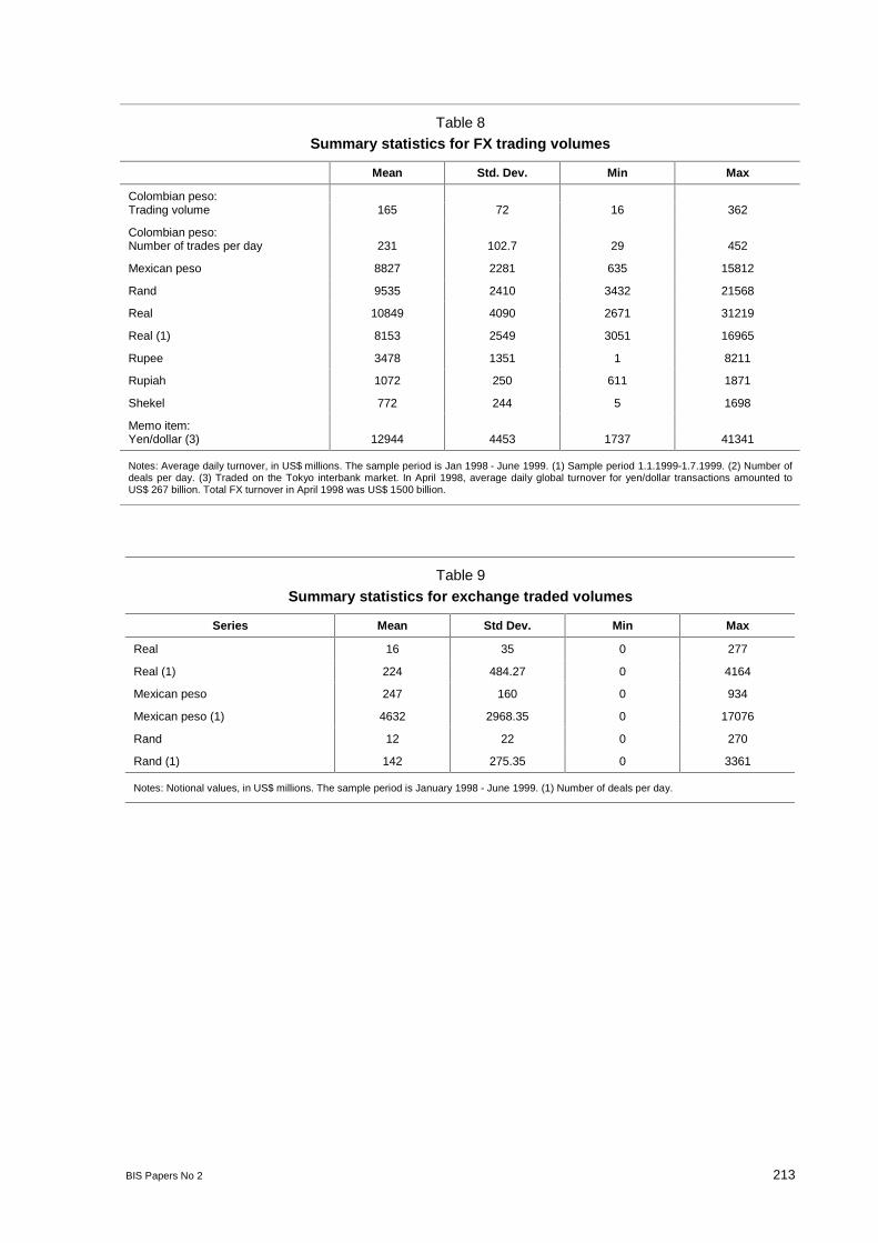
BIS Papers No 2 213
Table 8Summary statistics for FX trading volumes
Mean Std. Dev. Min Max
Colombian peso:Trading volume 165 72 16 362
Colombian peso:Number of trades per day 231 102.7 29 452
Mexican peso 8827 2281 635 15812
Rand 9535 2410 3432 21568
Real 10849 4090 2671 31219
Real (1) 8153 2549 3051 16965
Rupee 3478 1351 1 8211
Rupiah 1072 250 611 1871
Shekel 772 244 5 1698
Memo item:Yen/dollar (3) 12944 4453 1737 41341
Notes: Average daily turnover, in US$ millions. The sample period is Jan 1998 - June 1999. (1) Sample period 1.1.1999-1.7.1999. (2) Number ofdeals per day. (3) Traded on the Tokyo interbank market. In April 1998, average daily global turnover for yen/dollar transactions amounted toUS$ 267 billion. Total FX turnover in April 1998 was US$ 1500 billion.
Table 9
Summary statistics for exchange traded volumes
Series Mean Std Dev. Min Max
Real 16 35 0 277
Real (1) 224 484.27 0 4164
Mexican peso 247 160 0 934
Mexican peso (1) 4632 2968.35 0 17076
Rand 12 22 0 270
Rand (1) 142 275.35 0 3361
Notes: Notional values, in US$ millions. The sample period is January 1998 - June 1999. (1) Number of deals per day.
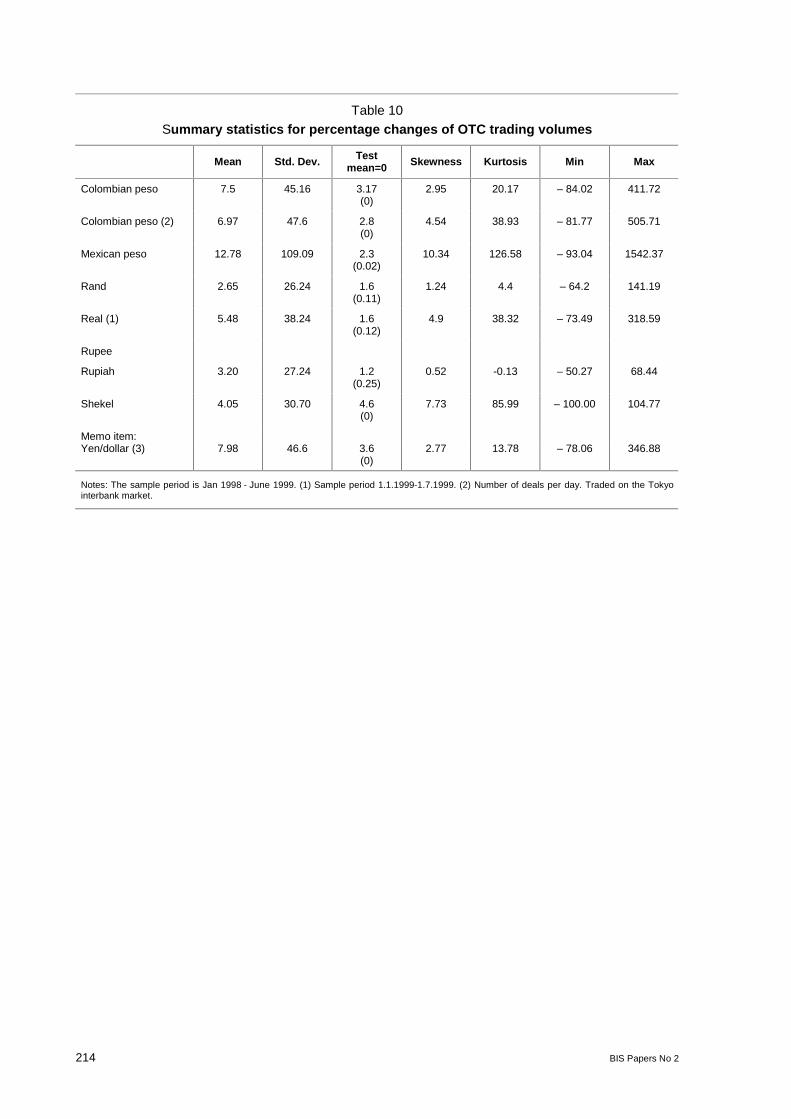
214 BIS Papers No 2
Table 10Summary statistics for percentage changes of OTC trading volumes
Mean Std. Dev. Testmean=0 Skewness Kurtosis Min Max
Colombian peso 7.5 45.16 3.17(0)
2.95 20.17 – 84.02 411.72
Colombian peso (2) 6.97 47.6 2.8(0)
4.54 38.93 – 81.77 505.71
Mexican peso 12.78 109.09 2.3(0.02)
10.34 126.58 – 93.04 1542.37
Rand 2.65 26.24 1.6(0.11)
1.24 4.4 – 64.2 141.19
Real (1) 5.48 38.24 1.6(0.12)
4.9 38.32 – 73.49 318.59
Rupee
Rupiah 3.20 27.24 1.2(0.25)
0.52 -0.13 – 50.27 68.44
Shekel 4.05 30.70 4.6(0)
7.73 85.99 – 100.00 104.77
Memo item:Yen/dollar (3) 7.98 46.6 3.6
(0)2.77 13.78 – 78.06 346.88
Notes: The sample period is Jan 1998 - June 1999. (1) Sample period 1.1.1999-1.7.1999. (2) Number of deals per day. Traded on the Tokyointerbank market.
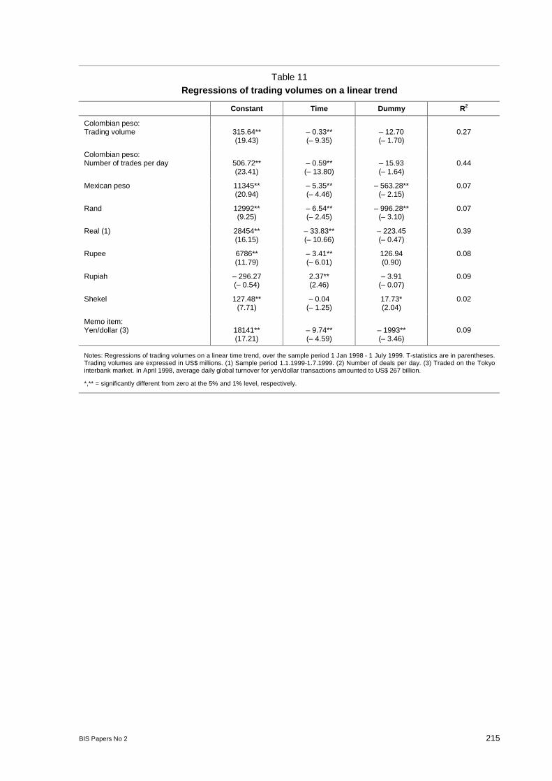
BIS Papers No 2 215
Table 11Regressions of trading volumes on a linear trend
Constant Time Dummy R2
Colombian peso:Trading volume 315.64**
(19.43)– 0.33**(– 9.35)
– 12.70(– 1.70)
0.27
Colombian peso:Number of trades per day 506.72**
(23.41)– 0.59**(– 13.80)
– 15.93(– 1.64)
0.44
Mexican peso 11345**(20.94)
– 5.35**(– 4.46)
– 563.28**(– 2.15)
0.07
Rand 12992**(9.25)
– 6.54**(– 2.45)
– 996.28**(– 3.10)
0.07
Real (1) 28454**(16.15)
– 33.83**(– 10.66)
– 223.45(– 0.47)
0.39
Rupee 6786**(11.79)
– 3.41**(– 6.01)
126.94(0.90)
0.08
Rupiah – 296.27(– 0.54)
2.37**(2.46)
– 3.91(– 0.07)
0.09
Shekel 127.48**(7.71)
– 0.04(– 1.25)
17.73*(2.04)
0.02
Memo item:Yen/dollar (3) 18141**
(17.21)– 9.74**(– 4.59)
– 1993**(– 3.46)
0.09
Notes: Regressions of trading volumes on a linear time trend, over the sample period 1 Jan 1998 - 1 July 1999. T-statistics are in parentheses.Trading volumes are expressed in US$ millions. (1) Sample period 1.1.1999-1.7.1999. (2) Number of deals per day. (3) Traded on the Tokyointerbank market. In April 1998, average daily global turnover for yen/dollar transactions amounted to US$ 267 billion.
*,** = significantly different from zero at the 5% and 1% level, respectively.
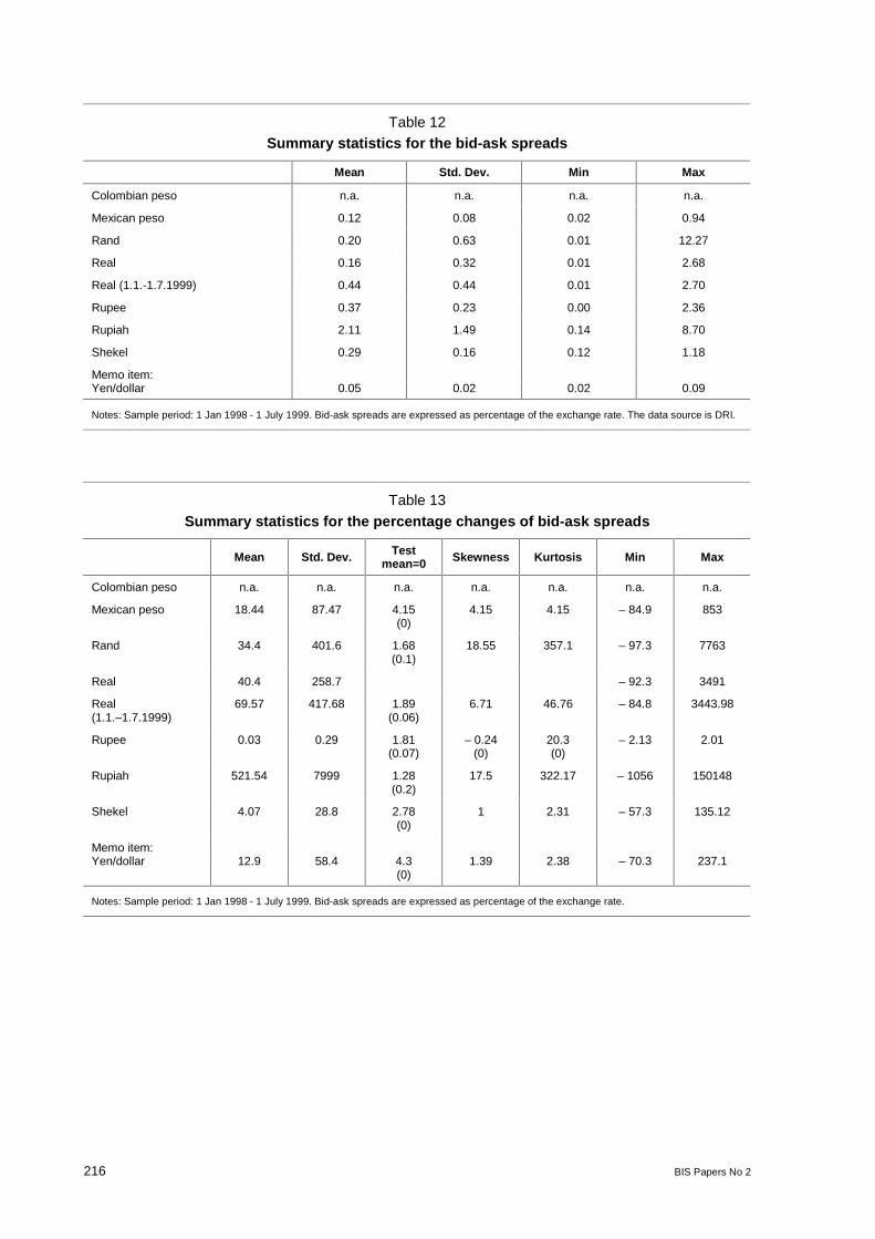
216 BIS Papers No 2
Table 12Summary statistics for the bid-ask spreads
Mean Std. Dev. Min Max
Colombian peso n.a. n.a. n.a. n.a.
Mexican peso 0.12 0.08 0.02 0.94
Rand 0.20 0.63 0.01 12.27
Real 0.16 0.32 0.01 2.68
Real (1.1.-1.7.1999) 0.44 0.44 0.01 2.70
Rupee 0.37 0.23 0.00 2.36
Rupiah 2.11 1.49 0.14 8.70
Shekel 0.29 0.16 0.12 1.18
Memo item:Yen/dollar 0.05 0.02 0.02 0.09
Notes: Sample period: 1 Jan 1998 - 1 July 1999. Bid-ask spreads are expressed as percentage of the exchange rate. The data source is DRI.
Table 13
Summary statistics for the percentage changes of bid-ask spreads
Mean Std. Dev. Testmean=0 Skewness Kurtosis Min Max
Colombian peso n.a. n.a. n.a. n.a. n.a. n.a. n.a.
Mexican peso 18.44 87.47 4.15(0)
4.15 4.15 – 84.9 853
Rand 34.4 401.6 1.68(0.1)
18.55 357.1 – 97.3 7763
Real 40.4 258.7 – 92.3 3491
Real(1.1.–1.7.1999)
69.57 417.68 1.89(0.06)
6.71 46.76 – 84.8 3443.98
Rupee 0.03 0.29 1.81(0.07)
– 0.24(0)
20.3(0)
– 2.13 2.01
Rupiah 521.54 7999 1.28(0.2)
17.5 322.17 – 1056 150148
Shekel 4.07 28.8 2.78(0)
1 2.31 – 57.3 135.12
Memo item:Yen/dollar 12.9 58.4 4.3
(0)1.39 2.38 – 70.3 237.1
Notes: Sample period: 1 Jan 1998 - 1 July 1999. Bid-ask spreads are expressed as percentage of the exchange rate.
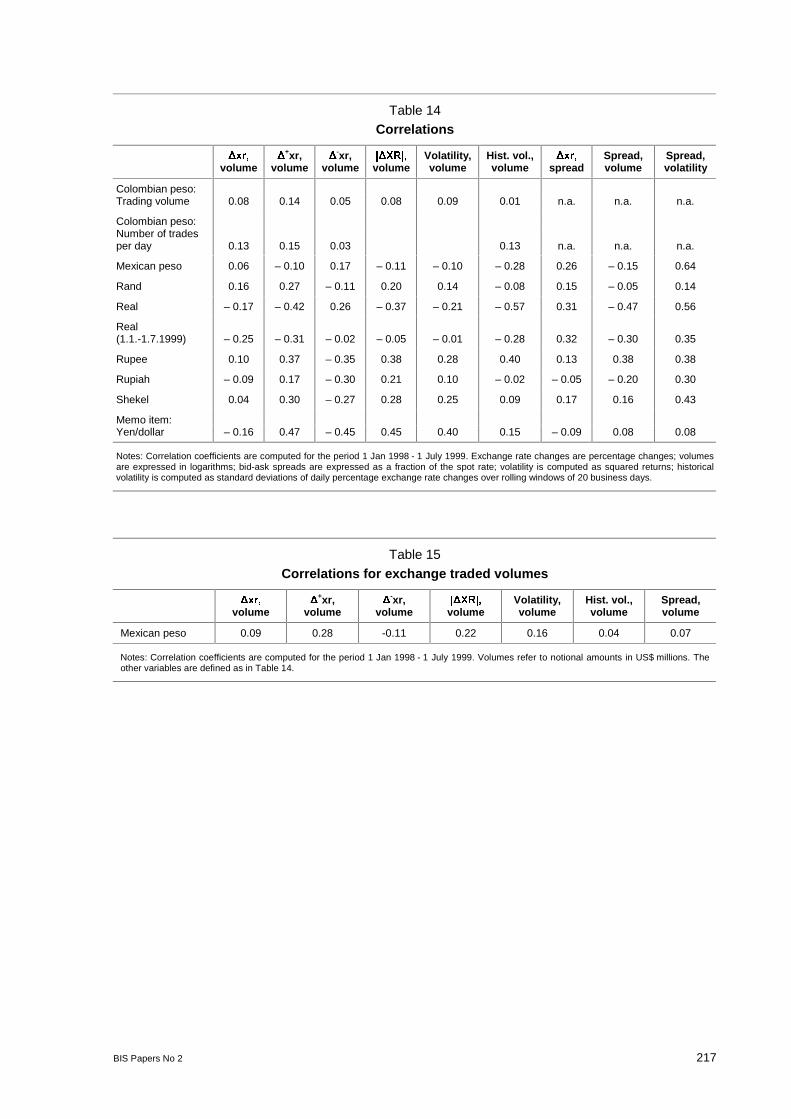
BIS Papers No 2 217
Table 14Correlations
[Uvolume
+xr,volume
-xr,volume
_ ;5_volume
Volatility,volume
Hist. vol.,volume
[Uspread
Spread,volume
Spread,volatility
Colombian peso:Trading volume 0.08 0.14 0.05 0.08 0.09 0.01 n.a. n.a. n.a.
Colombian peso:Number of tradesper day 0.13 0.15 0.03 0.13 n.a. n.a. n.a.
Mexican peso 0.06 – 0.10 0.17 – 0.11 – 0.10 – 0.28 0.26 – 0.15 0.64
Rand 0.16 0.27 – 0.11 0.20 0.14 – 0.08 0.15 – 0.05 0.14
Real – 0.17 – 0.42 0.26 – 0.37 – 0.21 – 0.57 0.31 – 0.47 0.56
Real(1.1.-1.7.1999) – 0.25 – 0.31 – 0.02 – 0.05 – 0.01 – 0.28 0.32 – 0.30 0.35
Rupee 0.10 0.37 – 0.35 0.38 0.28 0.40 0.13 0.38 0.38
Rupiah – 0.09 0.17 – 0.30 0.21 0.10 – 0.02 – 0.05 – 0.20 0.30
Shekel 0.04 0.30 – 0.27 0.28 0.25 0.09 0.17 0.16 0.43
Memo item:Yen/dollar – 0.16 0.47 – 0.45 0.45 0.40 0.15 – 0.09 0.08 0.08
Notes: Correlation coefficients are computed for the period 1 Jan 1998 - 1 July 1999. Exchange rate changes are percentage changes; volumesare expressed in logarithms; bid-ask spreads are expressed as a fraction of the spot rate; volatility is computed as squared returns; historicalvolatility is computed as standard deviations of daily percentage exchange rate changes over rolling windows of 20 business days.
Table 15
Correlations for exchange traded volumes
[Uvolume
+xr,volume
-xr,volume
_ ;5_volume
Volatility,volume
Hist. vol.,volume
Spread,volume
Mexican peso 0.09 0.28 -0.11 0.22 0.16 0.04 0.07
Notes: Correlation coefficients are computed for the period 1 Jan 1998 - 1 July 1999. Volumes refer to notional amounts in US$ millions. Theother variables are defined as in Table 14.

218 BIS Papers No 2
Table 16Volatility and trading volume: unconditional regressions
Constant Time trend Volume R2
Colombian peso – 3.86**(– 2.88)
0.0022**(4.16)
0.41*(2.14)
0.02
Colombian peso (2) – 1.62(– 0.83)
0.0008(0.42)
0.23*(2.46)
0.04
Mexican peso 2.89(1.54)
0.0002(0.44)
– 0.28(– 1.58)
0.00
Rand – 2.11(– 0.36)
– 0.02**(– 2.75)
2.17*(2.30)
0.06
Real(1) 121.19(1.75)
– 0.02(– 1.05)
– 10.80*(– 1.92)
0.07
Rupee 0.21(1.24)
– 0.001**(– 2.65)
0.05**(2.87)
0.04
Rupiah 20.10(0.76)
– 0.05(– 1.80)
5.01**(3.49)
0.07
Shekel – 1.06*(– 2.68)
0.0002*(2.06)
0.23**(2.75)
0.04
Memo item:Yen/dollar (3) – 32.18**
(– 2.98)0.0023*(2.45)
3.26**(3.03)
0.12
Notes: Regressions of exchange rate volatility, defined as squared returns, on a constant, a linear time trend and trading volumes (inlogarithms) over the sample period 1 Jan 1998 - 1 July 1999. T-statistics based on White’s asymptotically consistent standard errors are inparentheses. Coefficients on trading volumes are multiplied by 100. (1) Sample period 1.1.1999-1.7.1999. (2) Number of deals per day. (3)Traded on the Tokyo interbank market.
*,** = significantly different from zero at the 5% and 1% level, respectively.

BIS Papers No 2 219
Table 17Trading volumes and volatility
Constant ( ( R2
Colombian peso – 4.04– (2.47)
0.44(1.91)
0.34*(2.27)
0.02
Mexican peso 3.09(0.82)
– 0.28(– 0.78)
– 0.30(– 1.50)
0.00
Rand 7.50(0.66)
1.31(0.98)
3.08*(2.47)
0.07
Real (1) 69.93(1.04)
14.28(1.26)
– 2.83(– 0.62)
0.15
Rupee – 1.70**(– 2.74)
0.29**(3.16)
0.04**(2.91)
0.05
Rupiah 17.41(0.41)
5.32(1.19)
4.97**(2.96)
0.07
Shekel – 2.63**(– 2.87)
0.56**(2.91)
0.18**(2.65)
0.05
Memo item:Yen/dollar (2) – 27.27*
(– 2.04)2.78*(2.03)
3.20**(3.06)
0.11
Notes: Regressions of total volatility on a constant, a linear time trend, expected volumes and unexpected volumes. The sample period is 1 Jan1998 - 1 July 1999. Total volatility is defined as squared returns; log-volumes are decomposed into an expected and unexpected componentby using a fitted AR series and its residuals. T-statistics based on White’s asymptotically consistent standard errors are in parentheses. (1)Sample period 1.1.1999-1.7.1999. (2) Traded on the Tokyo interbank market.
*,** = significantly different from zero at the 5% and 1% level, respectively.
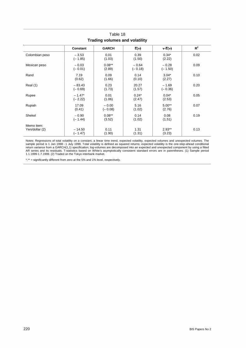
220 BIS Papers No 2
Table 18Trading volumes and volatility
Constant GARCH ( ( R2
Colombian peso – 3.53(– 1.85)
0.01(1.03)
0.39(1.50)
0.34*(2.22)
0.02
Mexican peso – 0.03(– 0.01)
0.08**(2.89)
– 0.64(– 0.18)
– 0.28(– 1.50)
0.09
Rand 7.19(0.62)
0.09(1.66)
0.14(0.10)
3.04*(2.27)
0.10
Real (1) – 83.43(– 0.69)
0.23(1.73)
20.27(1.57)
– 1.69(– 0.36)
0.20
Rupee – 1.47*(– 2.22)
0.01(1.06)
0.24*(2.47)
0.04*(2.53)
0.05
Rupiah 17.09(0.41)
– 0.00(– 0.08)
5.16(1.02)
5.00**(2.76)
0.07
Shekel – 0.90(– 1.44)
0.08**(3.52)
0.14(1.02)
0.08(1.51)
0.19
Memo item:Yen/dollar (2) – 14.50
(– 1.47)0.11
(1.90)1.31
(1.31)2.93**(3.23)
0.13
Notes: Regressions of total volatility on a constant, a linear time trend, expected volatility, expected volumes and unexpected volumes. Thesample period is 1 Jan 1998 - 1 July 1999. Total volatility is defined as squared returns; expected volatility is the one-step-ahead conditionalreturn variance from a GARCH(1,1) specification; log-volumes are decomposed into an expected and unexpected component by using a fittedAR series and its residuals. T-statistics based on White’s asymptotically consistent standard errors are in parentheses. (1) Sample period1.1.1999-1.7.1999. (2) Traded on the Tokyo interbank market.
*,** = significantly different from zero at the 5% and 1% level, respectively.

BIS Papers No 2 221
Table 19Spreads, trading volumes and volatility
Constant GARCH ( ( R2
Colombian peso n.a. n.a. n.a. n.a. n.a.
Mexican peso 0.47**(2.83)
0.01**(5.32)
– 0.05(– 2.65)
– 0.01(– 1.21)
0.20
Rand 0.96(1.42)
0.01(1.50)
– 0.10(– 1.45)
– 0.16(– 1.09)
0.05
Real(1) – 0.10(– 0.06)
0.01**(7.31)
0.02(0.13)
– 0.26(– 0.99)
0.47
Rupee 0.15(0.22)
0.03**(6.81)
0.01(0.16)
0.02(1.61)
0.22
Rupiah 7.77(1.73)
0.01*(2.28)
– 1.01(– 1.55)
– 0.44(– 1.74)
0.10
Shekel 0.23*(2.13)
0.03**(14.40)
– 0.03(– 1.42)
– 0.01(– 0.95)
0.62
Memo item:yen/dollar (2) 0.08
(1.18)0.00
(1.25)– 0.00
(– 0.48)0.00
(0.54)0.02
Notes: Regressions of bid-ask spreads on expected volatility, expected volumes and unexpected volumes estimated over the sample period 1Jan 1998 - 1 July 1999. Total volatility is defined as squared returns; expected volatility is the one-step-ahead conditional return variance froma GARCH(1,1) specification; volumes are decomposed into an expected and unexpected component by using a fitted AR(1) series and itsresiduals. T-statistics based on White’s asymptotically consistent standard errors are in parentheses. (1) Sample period 1.1.1999-1.7.1999. (2)Traded on the Tokyo interbank market.
*,** = significantly different from zero at the 5% and 1% level, respectively.
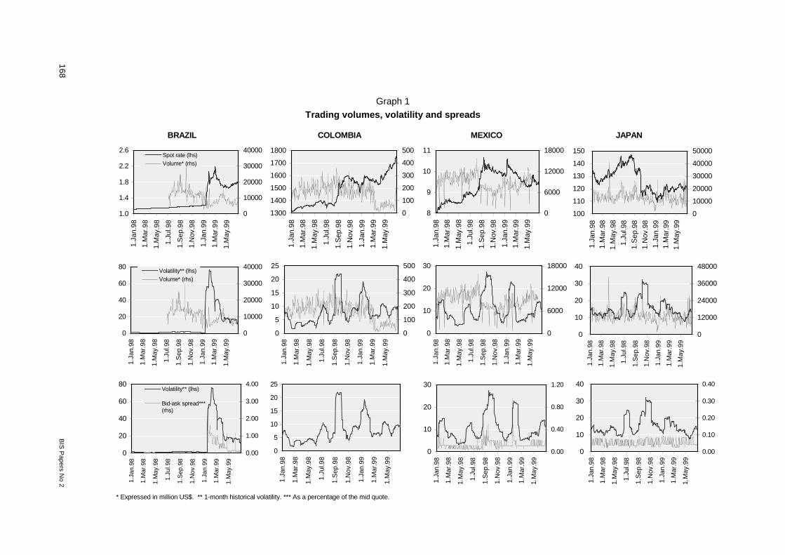
Graph 1
Trading volumes, volatility and spreads
BRAZIL COLOMBIA MEXICO JAPAN
* Expressed in million US$. ** 1-month historical volatility. *** As a percentage of the mid quote.
1.0
1.4
1.8
2.2
2.6
1.Ja
n .9 8
1.M
a r. 9
8
1 .M
a y. 9
8
1 .Ju
l. 98
1 .S
ep.9
8
1 .N
ov.9
8
1.Ja
n.99
1.M
ar.9
9
1.M
a y.9
9
0
10000
20000
30000
40000Spot rate (lhs)Volume* (rhs)
0
20
40
60
80
1.Ja
n.98
1.M
a r.9
8
1.M
ay.9
8
1 .Ju
l. 98
1 .S
ep.9
8
1 .N
ov.9
8
1.J a
n.9 9
1 .M
a r.9
9
1.M
a y.9
9
0
10000
20000
30000
40000Volatility** (lhs)
Volume* (rhs)
0
20
40
60
80
1.Ja
n.9 8
1 .M
ar.9
8
1 .M
ay.9
8
1.Ju
l.98
1 .S
ep.9
8
1 .N
ov.9
8
1 .J a
n .99
1.M
a r.9
9
1.M
a y.9
9
0.00
1.00
2.00
3.00
4.00Volatility** (lhs)
Bid-ask spread***(rhs)
1300
1400
1500
1600
1700
1800
1.Ja
n.98
1.M
ar.9
8
1 .M
a y. 9
8
1.Ju
l.98
1 .S
ep.9
8
1.N
o v.9
8
1 .Ja
n .9 9
1 .M
a r.9
9
1.M
ay.9
9
0
100
200
300
400
500
0
5
10
15
20
25
1.Ja
n.9 8
1 .M
a r.9
8
1 .M
a y. 9
8
1.J u
l.98
1.S
e p. 9
8
1.N
o v. 9
8
1.Ja
n.99
1.M
a r.9
9
1.M
a y. 9
9
0
100
200
300
400
500
0
5
10
15
20
25
1.Ja
n .98
1 .M
ar.9
8
1.M
a y. 9
8
1.Ju
l.98
1 .S
ep.9
8
1.N
o v. 9
8
1.Ja
n.99
1 .M
ar.9
9
1 .M
a y. 9
9
8
9
10
11
1.Ja
n .9 8
1 .M
a r. 9
8
1 .M
a y. 9
8
1 .J u
l .98
1 .S
ep.9
8
1 .N
ov.9
8
1.Ja
n.99
1 .M
a r. 9
9
1 .M
a y. 9
9
0
6000
12000
18000
0
10
20
30
1.Ja
n .9 8
1 .M
a r.9
8
1.M
ay.9
8
1 .J u
l. 98
1 .S
ep.9
8
1.N
o v. 9
8
1 .J a
n .9 9
1 .M
ar.9
9
1.M
a y. 9
9
0
6000
12000
18000
0
10
20
30
1.Ja
n .9 8
1.M
ar. 9
8
1.M
a y. 9
8
1 .J u
l .98
1.S
e p.9
8
1.N
o v. 9
8
1.J a
n .9 9
1.M
ar.9
9
1.M
ay.9
9
0.00
0.40
0.80
1.20
100
110
120
130
140
150
1.Ja
n .9 8
1 .M
ar.9
81 .
Ma y
. 98
1 .J u
l .98
1 .S
e p. 9
81.
No v
.98
1.Ja
n.99
1.M
a r. 9
91.
May
.99
0
10000
20000
30000
40000
50000
0
10
20
30
40
1.Ja
n.9 8
1 .M
ar.9
8
1 .M
a y.9
8
1 .J u
l .98
1 .S
ep.9
8
1 .N
o v.9
8
1 .J a
n .9 9
1 .M
ar.9
9
1 .M
ay.9
9
0
12000
24000
36000
48000
0
10
20
30
40
1.Ja
n.98
1.M
a r. 9
8
1 .M
ay.9
8
1 .J u
l .98
1.S
e p. 9
8
1.N
ov.9
8
1 .J a
n .9 9
1 .M
a r.9
9
1.M
a y.9
9
0.00
0.10
0.20
0.30
0.40
168B
IS P
apers No 2
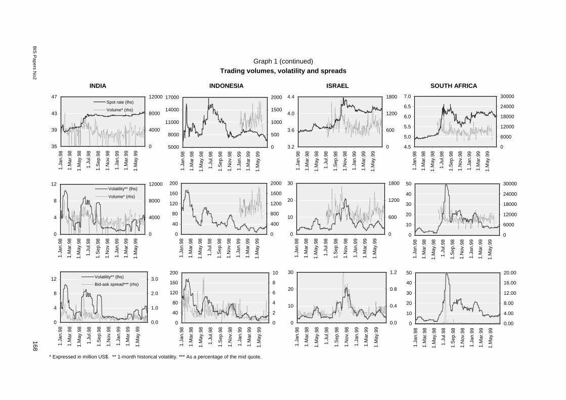
Graph 1 (continued)Trading volumes, volatility and spreads
INDIA INDONESIA ISRAEL SOUTH AFRICA
* Expressed in million US$. ** 1-month historical volatility. *** As a percentage of the mid quote.
35
39
43
47
1.Ja
n .9 8
1.M
ar. 9
8
1 .M
ay.9
8
1.J u
l.98
1.S
e p.9
8
1 .N
ov.9
8
1.J a
n.99
1 .M
a r.9
9
1.M
ay.9
9
0
4000
8000
12000Spot rate (lhs)
Volume* (rhs)
0
4
8
12
1.Ja
n.9 8
1 .M
ar.9
8
1 .M
a y. 9
8
1.Ju
l.98
1 .S
ep.9
8
1 .N
o v. 9
8
1.Ja
n.99
1 .M
a r.9
9
1.M
ay.9
9
0
4000
8000
12000Volatility** (lhs)
Volume* (rhs)
0
4
8
12
1.Ja
n.9 8
1 .M
ar.9
8
1 .M
ay.9
8
1 .J u
l. 98
1 .S
ep.9
8
1 .N
ov.9
8
1 .J a
n .9 9
1.M
a r. 9
9
1.M
a y.9
9
0.0
1.0
2.0
3.0Volatility** (lhs)
Bid-ask spread*** (rhs)
0
40
80
120
160
2001.
Jan .
9 8
1.M
a r. 9
8
1 .M
ay.9
8
1 .J u
l .98
1 .S
e p. 9
8
1.N
o v.9
8
1 .J a
n .9 9
1.M
a r. 9
9
1 .M
ay.9
9
0
400
800
1200
1600
2000
0
40
80
120
160
200
1.Ja
n.98
1 .M
a r.9
8
1 .M
a y. 9
8
1 .J u
l.98
1 .S
e p.9
8
1.N
o v. 9
8
1.J a
n.9 9
1 .M
ar.9
9
1 .M
ay.9
9
0
2
4
6
8
10
3.2
3.6
4.0
4.4
1.Ja
n .9 8
1 .M
ar.9
8
1.M
a y. 9
8
1 .Ju
l.98
1 .S
ep.9
8
1.N
o v. 9
8
1 .Ja
n .9 9
1.M
ar. 9
9
1 .M
a y.9
9
0
600
1200
1800
0
10
20
30
1.Ja
n.98
1 .M
ar.9
8
1 .M
a y.9
8
1 .J u
l. 98
1 .S
ep.9
8
1 .N
ov.9
8
1 .Ja
n .99
1 .M
a r.9
9
1 .M
a y.9
9
0
600
1200
1800
0
10
20
30
1.Ja
n .9 8
1.M
a r. 9
8
1 .M
a y. 9
8
1 .J u
l .98
1 .S
ep.9
8
1.N
ov.9
8
1.Ja
n.99
1 .M
ar.9
9
1.M
ay.9
9
0.0
0.4
0.8
1.2
4.5
5.0
5.5
6.0
6.5
7.0
1.Ja
n.98
1.M
ar. 9
8
1 .M
a y. 9
8
1 .Ju
l. 98
1.S
e p. 9
8
1 .N
o v.9
8
1 .Ja
n .9 9
1 .M
ar.9
9
1.M
a y.9
9
0
6000
12000
18000
24000
30000
0
10
20
30
40
50
1.Ja
n .9 8
1 .M
ar.9
8
1 .M
a y. 9
8
1.Ju
l.98
1 .S
ep.9
8
1 .N
o v. 9
8
1 .Ja
n .99
1.M
a r. 9
9
1 .M
ay.9
9
0
6000
12000
18000
24000
30000
0
10
20
30
40
50
1.Ja
n.98
1 .M
a r. 9
8
1.M
ay.9
8
1 .J u
l .98
1 .S
e p. 9
8
1 .N
ov.9
8
1 .J a
n .9 9
1 .M
ar.9
9
1 .M
a y. 9
9
0.00
4.00
8.00
12.00
16.00
20.00
5000
8000
11000
14000
17000
1.Ja
n.98
1.M
a r. 9
8
1.M
ay.9
8
1 .J u
l .98
1.S
e p. 9
8
1 .N
ov.9
8
1 .J a
n .9 9
1 .M
ar.9
9
1 .M
a y. 9
9
0
500
1000
1500
2000
BIS
Papers N
o2168

224 BIS Papers No 2
Graph 2Trading volumes and volatility in selected emerging markets
Korean won
0
1000
2000
3000
4000
5000
6000
7000
8000
9000
1995:01 1996:01 1997:01 1998:01 1999:01 2000:01
020406080100120140160180200
Brazilian real
0
2000
4000
6000
8000
10000
12000
1995:01 1996:01 1997:01 1998:01 1999:01 2000:01
0
10
20
30
40
50
60
70
80
Colombian peso
0
100
200
300
1995:01 1996:01 1997:01 1998:01 1999:01 2000:01
0.00
5.00
10.00
15.00
20.00
25.00
30.00
South African rand
0
1000
2000
3000
4000
5000
6000
7000
8000
9000
1995:01 1996:01 1997:01 1998:01 1999:01 2000:01
0
10
20
30
40
50
60
70
80
Indonesian rupiah
0
1000
2000
3000
4000
5000
6000
7000
8000
9000
1995:01 1996:01 1997:01 1998:01 1999:01 2000:01
020406080100120140160180200
Indian rupee
0
1000
2000
3000
4000
5000
1995:01 1996:01 1997:01 1998:01 1999:01 2000:01
0
10
20
30
40
50
60
70
80
Mexican peso
0
2000
4000
6000
8000
10000
12000
1995:01 1996:01 1997:01 1998:01 1999:01 2000:010
10
20
30
40
50
60
70
80
Israeli shekel
0
200
400
600
800
1000
1200
1995:01 1996:01 1997:01 1998:01 1999:01 2000:010.00
5.00
10.00
15.00
20.00
25.00
30.00
Notes: Trading volumes refer to local turnover in the domestic currency, per trading day in themonth shown (in millions of US$). In the case of Mexican and Brazil, turnover includes othercurrencies. Volatility is computed as one-month annualised standard deviation of percentagechanges in the exchange rate against the US dollar.
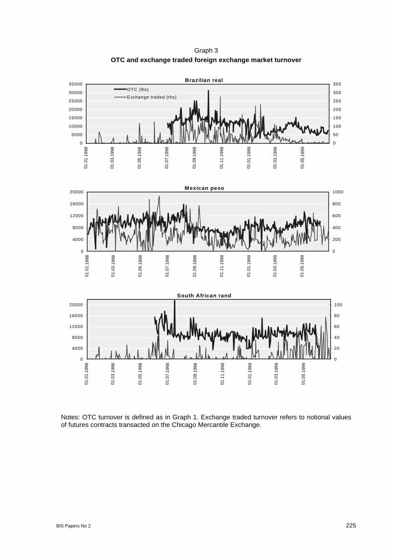
BIS Papers No 2 225
Graph 3OTC and exchange traded foreign exchange market turnover
Brazilian real
0
5000
10000
15000
20000
25000
30000
3500001
.01.
1998
01.0
3.1 9
9 8
0 1.0
5.19
98
0 1.0
7 .19
98
0 1.0
9.19
98
0 1. 1
1 .19
9 8
0 1.0
1 .1 9
9 9
0 1. 0
3 .19
9 9
0 1.0
5 .1 9
9 9
0
50
100
150
200
250
300
350OTC (lhs)
Exchange traded (rhs)
Mexican peso
0
4000
8000
12000
16000
20000
01.0
1 .19
98
0 1.0
3 .19
98
0 1. 0
5 .1 9
9 8
01.0
7.1 9
9 8
01.0
9.1 9
98
0 1.1
1 .19
98
0 1. 0
1 .1 9
9 9
0 1. 0
3 .1 9
9 9
01.0
5.1 9
9 9
0
200
400
600
800
1000
South African rand
0
4000
8000
12000
16000
20000
01.0
1 .1 9
9 8
0 1. 0
3 .19
9 8
0 1.0
5 .1 9
9 8
01.0
7.1 9
9 8
0 1.0
9 .1 9
9 8
01.1
1.1 9
9 8
01.0
1.1 9
99
01.0
3 .1 9
9 9
01.0
5.1 9
9 9
0
20
40
60
80
100
Notes: OTC turnover is defined as in Graph 1. Exchange traded turnover refers to notional valuesof futures contracts transacted on the Chicago Mercantile Exchange.
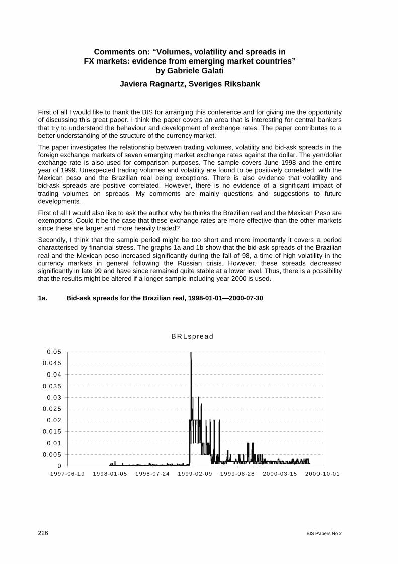
226 BIS Papers No 2
Comments on: “Volumes, volatility and spreads inFX markets: evidence from emerging market countries”
by Gabriele Galati
Javiera Ragnartz, Sveriges Riksbank
First of all I would like to thank the BIS for arranging this conference and for giving me the opportunityof discussing this great paper. I think the paper covers an area that is interesting for central bankersthat try to understand the behaviour and development of exchange rates. The paper contributes to abetter understanding of the structure of the currency market.
The paper investigates the relationship between trading volumes, volatility and bid-ask spreads in theforeign exchange markets of seven emerging market exchange rates against the dollar. The yen/dollarexchange rate is also used for comparison purposes. The sample covers June 1998 and the entireyear of 1999. Unexpected trading volumes and volatility are found to be positively correlated, with theMexican peso and the Brazilian real being exceptions. There is also evidence that volatility andbid-ask spreads are positive correlated. However, there is no evidence of a significant impact oftrading volumes on spreads. My comments are mainly questions and suggestions to futuredevelopments.
First of all I would also like to ask the author why he thinks the Brazilian real and the Mexican Peso areexemptions. Could it be the case that these exchange rates are more effective than the other marketssince these are larger and more heavily traded?
Secondly, I think that the sample period might be too short and more importantly it covers a periodcharacterised by financial stress. The graphs 1a and 1b show that the bid-ask spreads of the Brazilianreal and the Mexican peso increased significantly during the fall of 98, a time of high volatility in thecurrency markets in general following the Russian crisis. However, these spreads decreasedsignificantly in late 99 and have since remained quite stable at a lower level. Thus, there is a possibilitythat the results might be altered if a longer sample including year 2000 is used.
1a. Bid-ask spreads for the Brazilian real, 1998-01-01—2000-07-30
B R Lspread
0
0.005
0.01
0 .015
0.02
0 .025
0.03
0 .035
0.04
0 .045
0.05
1997-06-19 1998-01-05 1998-07-24 1999-02-09 1999-08-28 2000-03-15 2000-10-01
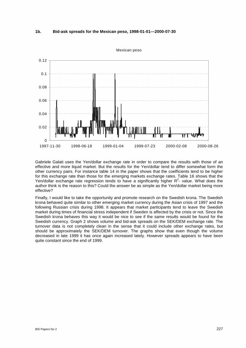
BIS Papers No 2 227
1b. Bid-ask spreads for the Mexican peso, 1998-01-01—2000-07-30
Mexican peso
0
0.02
0.04
0.06
0.08
0.1
0.12
1997-11-30 1998-06-18 1999-01-04 1999-07-23 2000-02-08 2000-08-26
Gabriele Galati uses the Yen/dollar exchange rate in order to compare the results with those of aneffective and more liquid market. But the results for the Yen/dollar tend to differ somewhat form theother currency pairs. For instance table 14 in the paper shows that the coefficients tend to be higherfor this exchange rate than those for the emerging markets exchange rates. Table 16 shows that theYen/dollar exchange rate regression tends to have a significantly higher R2- value. What does theauthor think is the reason to this? Could the answer be as simple as the Yen/dollar market being moreeffective?
Finally, I would like to take the opportunity and promote research on the Swedish krona. The Swedishkrona behaved quite similar to other emerging market currency during the Asian crisis of 1997 and thefollowing Russian crisis during 1998. It appears that market participants tend to leave the Swedishmarket during times of financial stress independent if Sweden is affected by the crisis or not. Since theSwedish krona behaves this way it would be nice to see if the same results would be found for theSwedish currency. Graph 2 shows volume and bid-ask spreads on the SEK/DEM exchange rate. Theturnover data is not completely clean in the sense that it could include other exchange rates, butshould be approximately the SEK/DEM turnover. The graphs show that even though the volumedecreased in late 1999 it has once again increased lately. However spreads appears to have beenquite constant since the end of 1999.
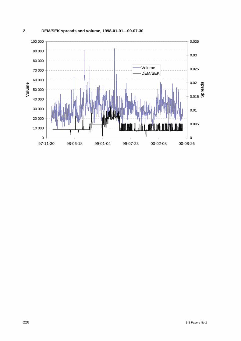
228 BIS Papers No 2
2. DEM/SEK spreads and volume, 1998-01-01—00-07-30
0
10 000
20 000
30 000
40 000
50 000
60 000
70 000
80 000
90 000
100 000
97-11-30 98-06-18 99-01-04 99-07-23 00-02-08 00-08-26
Vo
lum
e
0
0.005
0.01
0.015
0.02
0.025
0.03
0.035
Sp
read
s
VolumeDEM/SEK
BIS Papers No 2 229
Comments on “Trading volume, volatility and spreadsin FX markets: evidence from emerging market countries”
by Gabriele Galati
Alain Chaboud, Federal Reserve System
The nature of the interaction between volume, volatility and the bid-ask spread in foreign exchangemarkets is still poorly understood, and Gabriele Galati’s paper makes excellent use of a new set oftransaction volume data to shed light on the subject. The paper provides a test of what has becomeknown as the “mixture of distributions hypothesis,” which predicts that trading volume and volatility,simultaneously driven by the arrival of information, should be positively correlated. Using data forseven currencies of large emerging market economies, the paper offers support for that prediction,with the important exceptions of the Brazilian real and the Mexican peso. It also finds a positivecorrelation between volatility and bid-offer spreads, in line with inventory cost models. I offer a fewremarks on the analysis of the link between volume and volatility, and briefly touch on the subject offoreign exchange turnover data.
The study of the correlation between volatility and volume in this paper is rendered more interesting,but perhaps also more difficult, by the sample period of the study, 1998 and 1999, during which thefinancial markets of many emerging economies experienced turmoil. In that light, the failure of theBrazilian and Mexican currency markets to show a positive correlation between volume and volatility isnot altogether a surprise. It may not be much of a stretch to think that volatility and volume couldexhibit a positive relation only up to a certain level of volatility, with the correlation becoming negativeas volatility grows so large that many investors withdraw from the particular market. The predictions ofthe mixture of distributions hypothesis model would then be realised in “normal” market conditions, butnot in turbulent market conditions. This (unproven) scenario may be easier to swallow for the case ofemerging market currencies than for major currencies, but the sharp movement of the dollar/yenexchange rate in October 1998, reportedly accompanied by (likely in part caused by) thin marketconditions, is one recent example of this type of phenomenon occurring in a major market. One couldperhaps then interpret positive correlation between volume and volatility as a sign of a “healthy” orliquid markets, while the presence of negative correlation between volume and volatility could be takenas a symptom of inadequate liquidity. If such a non-linear relationship exists between volatility andvolume, simple linear regression techniques may not be fully adequate for proper inference, and, giventhe interesting results in the present paper, this may constitute a good opportunity for further research.
As is commonly done, the volatility measure used in this paper is based on net daily changes inexchange rates, matching the daily frequency of the turnover series. While this may appear to be avirtue, it would perhaps be preferable to use a volatility measure that better reflects the cumulativeamount of price movement over the trading day and not just the net movement. This would be more inthe spirit of the mixture of distributions hypothesis, where the arrival of each new piece of informationresults in both trading activity and movement in the price. With the daily turnover data representing thesum of all trading activity, matching them with a cumulative measure of price movement would avoid acase where, for instance, two salient pieces of news on the same day moved the exchange ratesharply but in opposite directions, yielding both a high trading volume and a misleadingly low measureof volatility. As an alternative measure of volatility, one could use the daily sum of absolute five -minute exchange rate movements, or some other estimate of integrated volatility. If high-frequencyprice data are unavailable, using the daily high-low range instead of the daily return as a measure ofvolatility has been shown to be a step in the right direction.
In a very interesting aside, the paper reports extremely low correlation coefficients between turnover inthree of the domestic spot markets in the study and corresponding futures markets turnover from theChicago Mercantile Exchange. Though the correlation coefficients may be affected by the very lowliquidity of those particular futures contracts, this finding still raises a (large red) flag, as currencyfutures turnover data have been widely used as a proxy for spot turnover data. For spot currencymarkets, over-the-counter and highly decentralised, transaction volume data for most currency pairshave generally been very difficult if not impossible to obtain. Several researchers have displayed greatingenuity and patience in assembling data sets such as the one in this study, but all these data havebeen limited in time and scope. The widespread use of electronic trading for most interdealertransactions in recent years carries with it hope that comprehensive high-frequency transaction datafor most major currency pairs may soon be available for research.

BIS Papers No 2 233
Sending the herd off the cliff edge:the disturbing interaction between herding andmarket-sensitive risk management practices1
Avinash Persaud, State Street
Summary
In the international financial arena, G7 policymakers chant three things: more market-sensitive riskmanagement, stronger prudential standards and improved transparency. The message is that we donot need a new world order, but we can improve the workings of the existing one. While many believethis is an inadequate response to the financial crises of the last two decades, few argue against riskmanagement, prudence and transparency. Perhaps we should, especially with regards to market-sensitive risk management and transparency. The underlying idea behind this holy trinity is that itbetter equips markets to reward good behaviour and penalise the bad, across governments andmarket players. However, while the market is discerning in the long-run, there is now compellingevidence that in the short run, market participants find it hard to distinguish between the good and theunsustainable; they herd; and contagion is common.
Critically, in a herding environment, tighter market-sensitive risk management systems and moretransparency actually makes markets less stable and more prone to crisis. This perverse responsemay help to explain the growing instability of the financial system. Over the past ten years the systemhas been in crisis in almost four. In response, the emphasis on market sensitive risk managementpractices and transparency must be tempered rather than extended vis-a-vis credit ratings agenciesand the risk management of investors. The incentives of regulators should be realigned to include theimpact of herding behaviour on foreign markets as well as local institutions. Financial marketinstitutions should be encouraged to set aside collateral for systemic risk or to buy liquidity optionsfrom central banks during good times. Countries should facilitate the inflow of capital from investorswho herd least or leave slowly: foreign direct investors, equity portfolio investors and, surprisingly,hedge funds.
A cyclical debate
The debate on reform of the international financial system follows a cycle. In the middle of each crisis- and there have been at least six since the Debt Crisis which started in Mexico in 1982 - there aredeafening demands for the whole-scale reform of the entire international financial system. A fewmonths on from the end of each crisis and those demands fade. There were clear and presentparallels between calls made in previous crises and those made in the thick of the last crisis, for theIMF to become a lender of last resort, injecting substantial liquidity in times of crisis, and for hedgefunds to be regulated. Every crisis inspires plans for a new financial architecture and as the crisisends, most of these plans are tidied away.
1This essay won first prize in the Institute of International Finance’s Jacques de Larosiere Awards in Global Finance 2000.
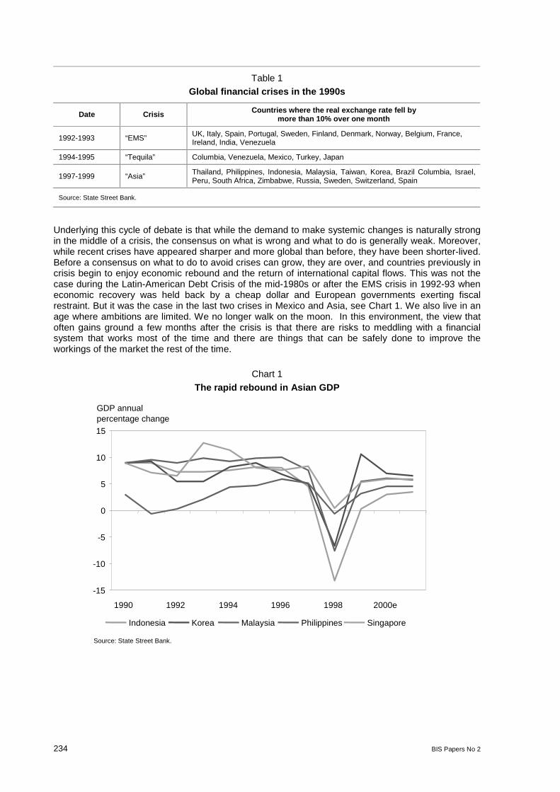
234 BIS Papers No 2
Table 1Global financial crises in the 1990s
Date Crisis Countries where the real exchange rate fell bymore than 10% over one month
1992-1993 “EMS” UK, Italy, Spain, Portugal, Sweden, Finland, Denmark, Norway, Belgium, France,Ireland, India, Venezuela
1994-1995 “Tequila” Columbia, Venezuela, Mexico, Turkey, Japan
1997-1999 “Asia” Thailand, Philippines, Indonesia, Malaysia, Taiwan, Korea, Brazil Columbia, Israel,Peru, South Africa, Zimbabwe, Russia, Sweden, Switzerland, Spain
Source: State Street Bank.
Underlying this cycle of debate is that while the demand to make systemic changes is naturally strongin the middle of a crisis, the consensus on what is wrong and what to do is generally weak. Moreover,while recent crises have appeared sharper and more global than before, they have been shorter-lived.Before a consensus on what to do to avoid crises can grow, they are over, and countries previously incrisis begin to enjoy economic rebound and the return of international capital flows. This was not thecase during the Latin-American Debt Crisis of the mid-1980s or after the EMS crisis in 1992-93 wheneconomic recovery was held back by a cheap dollar and European governments exerting fiscalrestraint. But it was the case in the last two crises in Mexico and Asia, see Chart 1. We also live in anage where ambitions are limited. We no longer walk on the moon. In this environment, the view thatoften gains ground a few months after the crisis is that there are risks to meddling with a financialsystem that works most of the time and there are things that can be safely done to improve theworkings of the market the rest of the time.
Chart 1
The rapid rebound in Asian GDP
-15
-10
-5
0
5
10
15
1990 1992 1994 1996 1998 2000e
Indonesia Korea Malaysia Philippines Singapore
GDP annualpercentage change
Source: State Street Bank.

BIS Papers No 2 235
The proposals that emerge post-crisis, therefore, tend to focus on making it easier for the market toreward good behaviour and penalise the bad. The emphasis is not on changing the rules of the game,but on strengthening the players: stronger risk management, more prudential standards and improvedtransparency. One of the key responses of the Interim Committee of the IMF to the latest crisis and thedesire to avoid a next one was the adoption on 26 September 1999 of a new Code of Good Practiceson Transparency in Monetary and Financial Policies. Incidentally, these measures are all relativelyinexpensive to implement. There is declining political support for large packages of tax-payers moneyto bail out foreign countries in trouble.
How more market-sensitive risk management can create risk
While many believe that market sensitive risk management, prudential standards and transparencyare probably not enough to avoid future crises, they believe these measures will probably help toprovide the right discipline for governments and can surely do no harm. These measures are likely tobe a positive force in the long run when markets are better at discerning between the good and bad.But in the short-run, there is growing evidence that market participants find it hard to discern betweenthe good and the unsustainable, they often herd and contagion from one crisis to another is common.The problem is that in a world of “herding”, tighter market-sensitive risk management regulations andimproved transparency can, perversely, turn events from bad to worse, creating volatility, reducingdiversification and triggering contagion. How can this happen?
Let us explore the interaction between herding, market-sensitive risk management and transparency inbank lending. It is important to note that bank lending remains a powerful feature of modern-daycrises. For example, the five Asian crisis countries - Thailand, Malaysia, South Korea, Indonesia andthe Philippines - received USD 47.8 billion in foreign bank loans in 1996. In 1997, banks withdrewUSD 29.9 billion, a net turnaround of almost USD 80 billion in one year. By contrast, equity portfolioflows remained positive throughout 1997, see “Portfolio Flow Indicator - Technical Document, StateStreet Bank and FDO Partners, 1999”.
The growing fashion in risk management, supported by the Basel Committee on Banking Supervision,is a move away from discretionary judgements about risk and a move to more quantitative and market-sensitive approaches (for an early reference see, the Supervisory Treatment of Market Risks, BaselCommittee on Banking Supervision, 1993). This is well illustrated by how banks now tend to managemarket risks by setting a DEAR limit - daily earnings at risk. DEAR answers the question: how muchcan I lose with, say, a 1% probability over the next day. It is calculated by taking the bank’s portfolio ofpositions and estimating the future distribution of daily returns based on past measures of marketcorrelation and volatility. Both rising volatility and rising correlation will increase the potential loss ofthe portfolio, increasing DEAR. Falling volatility and correlation will do the opposite. Banks set a DEARlimit: the maximum dollar amount they are prepared to put at risk of losing with a 1% probability. WhenDEAR exceeds the limit, the bank reduces exposure, often by switching into less volatile and lesscorrelated assets such as US dollar cash. (See RiskMetrics Technical Manual, RiskMetrics Group,London, 1999.)
By herding behaviour I mean that banks or investors like to buy what others are buying, sell whatothers are selling and own what others own. There are three main explanations for why bankers andinvestors herd. First, in a world of uncertainty, the best way of exploiting the information of others is bycopying what they are doing. Second, bankers and investors are often measured and rewarded byrelative performance so it literally does not pay a risk-averse player to stray too far from the pack.Third, investors and bankers are more likely to be sacked for being wrong and alone than being wrongand in company. (For further explanations of herding see Investor Behaviour in the October 1987Stock Market Crash: Survey Evidence by R Shiller, NBER discussion paper 2446, 1990.)
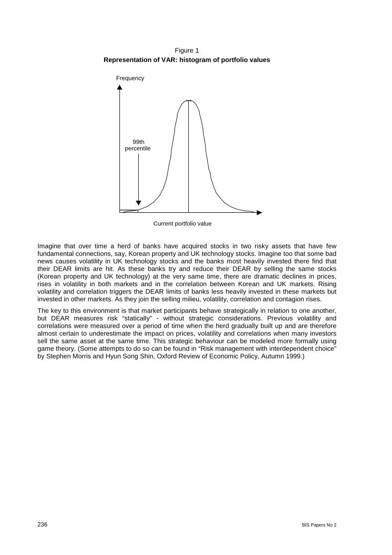
236 BIS Papers No 2
Figure 1Representation of VAR: histogram of portfolio values
Frequency
Current portfolio value
99thpercentile
Imagine that over time a herd of banks have acquired stocks in two risky assets that have fewfundamental connections, say, Korean property and UK technology stocks. Imagine too that some badnews causes volatility in UK technology stocks and the banks most heavily invested there find thattheir DEAR limits are hit. As these banks try and reduce their DEAR by selling the same stocks(Korean property and UK technology) at the very same time, there are dramatic declines in prices,rises in volatility in both markets and in the correlation between Korean and UK markets. Risingvolatility and correlation triggers the DEAR limits of banks less heavily invested in these markets butinvested in other markets. As they join the selling milieu, volatility, correlation and contagion rises.
The key to this environment is that market participants behave strategically in relation to one another,but DEAR measures risk “statically” - without strategic considerations. Previous volatility andcorrelations were measured over a period of time when the herd gradually built up and are thereforealmost certain to underestimate the impact on prices, volatility and correlations when many investorssell the same asset at the same time. This strategic behaviour can be modeled more formally usinggame theory. (Some attempts to do so can be found in “Risk management with interdependent choice”by Stephen Morris and Hyun Song Shin, Oxford Review of Economic Policy, Autumn 1999.)
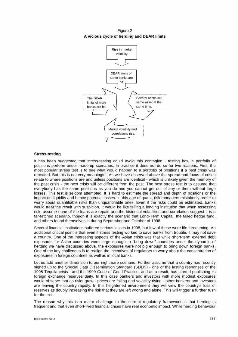
BIS Papers No 2 237
Figure 2A vicious cycle of herding and DEAR limits
Rise in marketvolatility
Several banks sellsame asset at thesame time.
Market volatility andcorrelations rise.
The DEARlimits of morebanks are hit.
DEAR limits ofsome banks are
hit
Stress-testing
It has been suggested that stress-testing could avoid this contagion - testing how a portfolio ofpositions perform under made-up scenarios. In practice it does not do so for two reasons. First, themost popular stress test is to see what would happen to a portfolio of positions if a past crisis wasrepeated. But this is not very meaningful. As we have observed above the spread and focus of crisesrelate to where positions are and unless positions are identical - which is unlikely given the memory ofthe past crisis - the next crisis will be different from the past. The best stress test is to assume thateverybody has the same positions as you do and you cannot get out of any or them without largelosses. This test is seldom attempted. It is hard to estimate the spread and depth of positions or theimpact on liquidity and hence potential losses. In this age of quant, risk managers mistakenly prefer toworry about quantifiable risks than unquantifiable ones. Even if the risks could be estimated, bankswould treat the result with suspicion. It would be like telling a lending institution that when assessingrisk, assume none of the loans are repaid and the historical volatilities and correlation suggest it is afar-fetched scenario, though it is exactly the scenario that Long-Term Capital, the failed hedge fund,and others found themselves in during September and October of 1998.
Several financial institutions suffered serious losses in 1998, but few of these were life threatening. Anadditional critical point is that even if stress testing worked to save banks from trouble, it may not savea country. One of the interesting aspects of the Asian crisis was that while short-term external debtexposures for Asian countries were large enough to “bring down” countries under the dynamic ofherding we have discussed above, the exposures were not big enough to bring down foreign banks.One of the key challenges is to realign the incentives of regulators to worry about the concentration ofexposures in foreign countries as well as in local banks.
Let us add another dimension to our nightmare scenario. Further assume that a country has recentlysigned up to the Special Data Dissemination Standard (SDDS) - one of the lasting responses of the1995 Tequila crisis - and the 1999 Code of Good Practice, and as a result, has started publishing itsforeign exchange reserves daily. In this case bankers and investors with more modest exposureswould observe that as risks grow - prices are falling and volatility rising - other bankers and investorsare leaving the country rapidly. In this heightened environment they will view the country’s loss ofreserves as doubly increasing the risk that they are left wrong and alone. This will trigger a further rushfor the exit.
The reason why this is a major challenge to the current regulatory framework is that herding isfrequent and that even short-lived financial crises have real economic impact. While herding behaviour
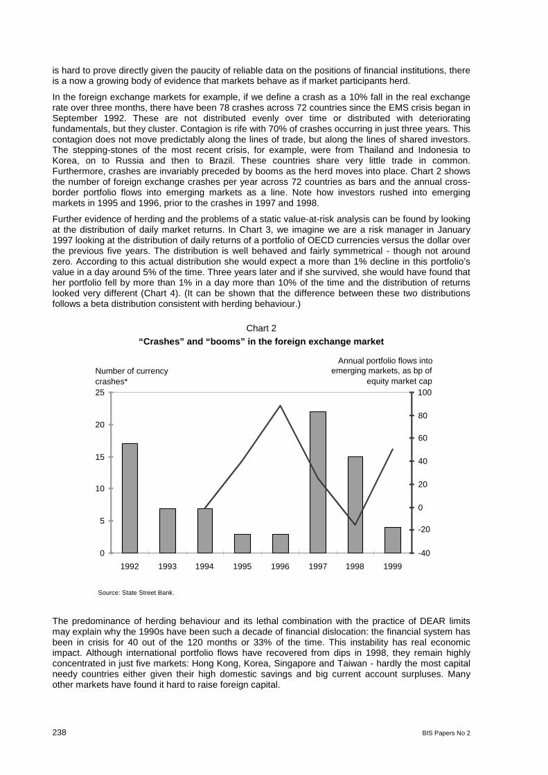
238 BIS Papers No 2
is hard to prove directly given the paucity of reliable data on the positions of financial institutions, thereis a now a growing body of evidence that markets behave as if market participants herd.
In the foreign exchange markets for example, if we define a crash as a 10% fall in the real exchangerate over three months, there have been 78 crashes across 72 countries since the EMS crisis began inSeptember 1992. These are not distributed evenly over time or distributed with deterioratingfundamentals, but they cluster. Contagion is rife with 70% of crashes occurring in just three years. Thiscontagion does not move predictably along the lines of trade, but along the lines of shared investors.The stepping-stones of the most recent crisis, for example, were from Thailand and Indonesia toKorea, on to Russia and then to Brazil. These countries share very little trade in common.Furthermore, crashes are invariably preceded by booms as the herd moves into place. Chart 2 showsthe number of foreign exchange crashes per year across 72 countries as bars and the annual cross-border portfolio flows into emerging markets as a line. Note how investors rushed into emergingmarkets in 1995 and 1996, prior to the crashes in 1997 and 1998.
Further evidence of herding and the problems of a static value-at-risk analysis can be found by lookingat the distribution of daily market returns. In Chart 3, we imagine we are a risk manager in January1997 looking at the distribution of daily returns of a portfolio of OECD currencies versus the dollar overthe previous five years. The distribution is well behaved and fairly symmetrical - though not aroundzero. According to this actual distribution she would expect a more than 1% decline in this portfolio’svalue in a day around 5% of the time. Three years later and if she survived, she would have found thather portfolio fell by more than 1% in a day more than 10% of the time and the distribution of returnslooked very different (Chart 4). (It can be shown that the difference between these two distributionsfollows a beta distribution consistent with herding behaviour.)
Chart 2
“Crashes” and “booms” in the foreign exchange market
0
5
10
15
20
25
1992 1993 1994 1995 1996 1997 1998 1999
-40
-20
0
20
40
60
80
100
Number of currencycrashes*
Annual portfolio flows intoemerging markets, as bp of
equity market cap
Source: State Street Bank.
The predominance of herding behaviour and its lethal combination with the practice of DEAR limitsmay explain why the 1990s have been such a decade of financial dislocation: the financial system hasbeen in crisis for 40 out of the 120 months or 33% of the time. This instability has real economicimpact. Although international portfolio flows have recovered from dips in 1998, they remain highlyconcentrated in just five markets: Hong Kong, Korea, Singapore and Taiwan - hardly the most capitalneedy countries either given their high domestic savings and big current account surpluses. Manyother markets have found it hard to raise foreign capital.

BIS Papers No 2 239
Chart 3Distribution of average daily dollar returns of an OECD
less US portfolio of currencies, 1992-96
0
50
100
150
200
250
300-0
.028
77
-0.0
2527
-0.0
2176
-0.0
1826
-0.0
1475
-0.0
1125
-0.0
0775
-0.0
0424
-0.0
0074
0.00
277
0.00
627
0.00
977
ore
Frequency
These financial crises also have a direct impact on GDP. For example, while there has been a strongrebound in GDP in 1999 in Asia in general and in South Korea in particular, the rebound has not offsetthe loss of GDP during the crisis period. One way of estimating the lost GDP of the Asian crisis is toestimate where GDP would be today if Asian economies had continued the more modest butsustainable growth rates experienced in the five years before their current account deficits began towiden in 1993-94. Were it not for the crisis and its preceding boom, GDP would be an aggregate ofUSD 130 billion higher in South Korea, Thailand, Malaysia and Indonesia. Another measure of thislasting impact is the elevation of poverty levels in Asia today compared with 1997.
Chart 4
Distribution of average daily dollar returns of an OECDless US portfolio of currencies, 1997-99
0
20
40
60
80
100
120
140
160
-0.0
1670
-0.0
1417
-0.0
1165
-0.0
0912
-0.0
0660
-0.0
0407
-0.0
0155
.000
97
.003
50
.006
02
.008
55
.011
07
.013
59
.016
12
Frequency

240 BIS Papers No 2
The paradox is that if one or two banks followed a DEAR limit and others did not, those banks wouldhave an effective risk management system that at the margin would support the financial system. Butif every bank were to follow the same approach, given that these banks follow each other into and outof markets, the DEAR limit would contribute to systemic risk. It is ironic therefore that the BaselCommittee on Banking Supervision is supporting the rapid adoption of these systems across all banksand encouraging investors to follow suit, for an early reference see “An internal model-based approachto market risk capital requirements”, Bank for International Settlements, Basel, 1995. There is a furtherparadox with transparency. The more herding investors and banks know about what each other are upto the more unstable markets may become. In the long run transparency and DEAR limits are a gooddevelopment, but they are harmful in the short-run in the context of herding behaviour.
What should policymakers and regulators do?
Herding presents a classic example of the need for intervention. The individual incentives of herdinginvestors create systemic risks. Moreover, if regulators were so coordinated that they behaved like oneglobal regulator, they would be best placed to make an intervention. Through the privileged formationthey have as a regulator of individual bank balance sheets they know when banks are herding. Thisrequires a different focus. Today regulators are warned by other regulators when banks in theirjurisdiction have exposures that threaten themselves, not whether banks around the world haveexposures which together threaten a foreign market and could become contagious.
However, if this information were made public, in the context of herding investors, random shockscould quickly evolve into financial crises. But how should regulators respond if they notice herding in aparticular market? They should require the bank to put aside an extra amount of capital for “strategicrisk” without specifying which markets carry that risk. Applying tighter risk management requirementsfor those specific markets in which the herd has appeared will only make the stampede more viciouswhen negative news strikes. Collateral requirements are like a tax on banks and are very unpopular.However, banks could be given the choice of either putting up strategic collateral from time to time, orby buying liquidity options from the central bank during good times.
Whether these solutions would work or not, the whole concept of market-sensitive risk managementpractices needs to be seriously reconsidered in the context of herding and the authorities shouldrethink their extension to the use of credit rating agencies and the risk management of long-terminvestors.
It is arguable that regulators have actually promoted herding through risk management systems. Theymay also have done so in their zeal for disclosure of bank positions and central bank reserves. Indeed,there is a role for one unregulated investor who is encouraged to buy near the bottom of marketsthrough the absence of risk, capital disclosure and credit concerns. Such investors would make thesystem safer but would be high risk and so should be restricted to those who can afford to lose. If thisinvestor had to be invented she would look something like a hedge fund. Interestingly, as the big-betting hedge funds have been undermined by the disclosure and credit policies of banks, marketliquidity has fallen and volatility has risen. Just as the big macro hedge funds fade away we may findthat they supported the market as much as they exploited it.
Those of you unable to stomach regulators promoting hedge funds will be relived to note that there areother kinds of flows that do not herd so much, foreign direct investment for example. Further, duringthe Mexican and Asian crises, equity portfolio flows also revealed less herding than bond flows. Itwould appear that bond investors are keen to get out before they are held in by a debt moratorium ororderly work out. This raises some interesting questions for those trying to build in burden-sharing andorderly work out provisions into bond constitutions.
Transparency in data and governance is clearly a good thing in the long-run and promotes the rightbehaviour of governments. Governments should be encouraged to disclose more information everymonth and quarter, but not on a daily basis. In an environment of herding investors, there is not agood case for insisting that countries release central bank reserve data with such high frequency. It istelling that during the EMS crisis, many of the developed countries that have just adopted the Code ofGood Practice on Transparency found it helpful to delay the monthly publication of their officialreserves or to camouflage its information for several months. Small vulnerable emerging markets willfind it even more helpful not to publish their reserves every day or every week and should not beforced to do so.
BIS Papers No 2 241
How safe was the “Safe Haven”?Financial market liquidity during the 1998 turbulences
Christian Upper, Deutsche Bundesbank 1
Summary
The turbulences in the international financial markets during the summer and autumn of 1998 put theprice formation and liquidity provision mechanism in many markets under severe strain. As part of thelarge-scale portfolio rebalancing that took place, investors shifted a large part of their holdings intocash and into instruments that were perceived as having a low risk and being highly liquid. One ofthese “safe havens” was the market for German government securities. The paper examines theliquidity of the secondary market for four German benchmark government bonds during this period.The analysis is based on a unique dataset provided by the German securities’ regulator, which coversevery single transaction of the four bonds in Germany. This feature is particularly attractive for thebond market, where OTC transactions account for most trading.
The volatility of yields of the four bonds more than doubled in the wake of the Russian devaluation on17 August 1998, and experienced a further peak in early October. It was accompanied by a wideningin the yield spread between the individual bonds, which soared to more than twenty basis points fromless than five basis points during the first half of the year. The cost of trading, as measured by theeffective spread, increased even in a “safe” haven like the market for ten year German governmentbonds, indicating a reduction in liquidity. Nevertheless, the market was able to handle a statisticallysignificantly higher than usual number of transactions and turnover. In this sense, liquidity provisionhas been remarkably effective in dealing with the turbulences.
Effective bid-ask spreads are positively related to unexpected trading volume, which should reflect theamount of private information in the market. Nevertheless, surprises volume cannot explain the surgein spreads that occurred during the turbulences.
1. Introduction
The turbulences in the international financial markets during the summer and autumn of 1998 put theprice formation and liquidity provision mechanism in many markets under severe strain. Both theInternational Monetary Fund and the Bank for International Settlements2 cite anecdotal evidence that“market liquidity dried up temporarily even in the deepest and most liquid markets as risks wererepriced and positions deleveraged”(IMF [1998]). As part of the large-scale portfolio rebalancing thattook place, investors shifted a large part of their holdings into cash and into instruments that wereperceived as having a low risk and being highly liquid. One of these “safe havens” was the market forGerman government securities. The purchases of German debt securities by non-residents, which hadaveraged some of 11.4 billion DM per month during the first half of 1998, soared to 34.5 billion DM inJuly and remained close to this level in August. Most of this increase went into bonds issued by theFederal government, in particular those with maturities around ten years, whose yields fellaccordingly.3 The safe-haven effect disappears from the data as the turbulences reached their climax
1Discussion paper 1/00, Economic Research Group of the Deutsche Bundesbank. Parts of the paper have been writtenduring a visit at the Bank of England’s Financial Intermediaries Division, which I thank for its hospitality. I am particularlygrateful to Charles Goodhart for helping me to arrange the visit and taking an active interest in its success. My work hasbenefited greatly from discussions with Torsten Arnswald, John Board, Dietrich Domanski, Heinz Herrmann,Manfred Kremer, Narayan Naik, Anthony Neuberger, Richard Payne, Victoria Saporta, Anne Vila and several staff at boththe Bundesbank and the Bank of England. It would not have been possible without the generous help of Patrick Umlauf andMichael Kollak of the Bundesamt für den Wertpapierhandel, who made the data available. I would also like to thankGerhard Klopf and Uwe Ullrich for valuable information on the institutional structure of the German bond market. Allremaining errors are mine. The discussion papers published in this series represent the authors’ personal opinions and donot necessarily reflect the views of the Deutsche Bundesbank.
2IMF (1998) and BIS (1999a).
3As a consequence, the spread between the benchmark government bonds and bonds issued by other institutions widenedsignificantly. See Deutsche Bundesbank (1998).

242 BIS Papers No 2
in early October. Purchases of German bonds by non-residents fell back to 8.6 billion DM inSeptember and were actually negative in October, when foreign investors reduced their holdings ofGerman bonds by 10 billion DM.
This paper analyses the evolution of prices and indicators for market liquidity during 1998 for fourbenchmark 10 year Bundesanleihen. These securities represent the most liquid and actively tradedsegment of the German fixed income market, and were the main beneficiary of the flight into quality. Inparticular, I focus on the question of how the turbulences affected market liquidity and price formation.In other words, how did the safe haven weather the storm? Beyond this immediate question, the paperintends to further our understanding of the mechanisms for the provision of liquidity in securitiesmarkets more generally, especially in periods of stress.
The market for Government debt is of particular concern to central banks for a number of reasons.4
Firstly, the prices of government securities provide important indicators for monetary policy, eg throughthe yield curve, and serve as benchmarks for the pricing of other securities. Such indicators will onlybe accurate if prices are efficient, ie if they accurately reflect all available information. If markets arenot liquid enough, then this may not be the case.
Secondly, government bonds are important hedging vehicles for market participants. A breakdown inmarket liquidity turns tradable assets turn into non-marketable loans or at least induces large changesin prices. This can lead to substantial losses for those market participants who rely on the ability toturn over positions quickly and at a low price. Upper bounds for the cost of a temporary interruption oftradability have been derived using an options pricing approach by Longstaff (1995). Such costs arisefrom investors not being able to optimally time their trades. The upper bounds are concave in the timeduring which the asset cannot be sold, indicating that the cost of illiquidity may be very high even if theperiod of non-tradability lasts only a short period of time.
In addition, continuous liquidity is the key assumption of standard option pricing and risk managementmodels, which are based on dynamic hedging strategies. If the underlying assets cannot easily betraded, then options can no longer be priced correctly and the riskiness of a portfolio cannot beassessed. While this does not directly impose a cost on investors, it contributes to a rise in uncertaintyabout their financial health and may trigger off massive sales or runs that could possibly call intoquestion the stability of the financial system. The prevention of such periods of illiquidity shouldtherefore be of serious concern to policymakers and central banks in their quest to safeguard financialstability.
A third reason for why central banks should be interested in the market for government bonds lies intheir role as fiscal agents. If secondary markets are not very liquid, then this may add to the borrowingcosts of the government. This cost of illiquidity can be substantial. For example, Amihud & Mendelson(1991) find that, after accounting for brokerage fees, the yield of US-Treasury Bills was on average 39basis points lower than that of Treasury Notes of the same residual maturity but with a bid-ask spreadabout four times as high.5
Market microstructure theory has identified three factors which affect liquidity in financial markets:order processing costs, inventory control considerations and adverse selection problems.6 Orderprocessing costs include exchange fees and taxes as well as the more immediate costs of handlingtransactions. They should be fairly constant over time unless changes in the microstructure of themarket or in technology take place, and are therefore an unlikely candidate when it comes toexplaining variations in market liquidity.
Inventory and adverse selection effects are much more likely to vary even in the short run. The formerarise from uncertainty about the order flow and thus the size of the inventory as well as fromuncertainty about future prices and hence the valuation of the portfolio.7 Adverse selection problemsarise when a group of investors has private information on the value of the asset and will want to trade
4This has been pointed out by several papers in BIS (1999b).
5They argue that the larger spread of the T-Notes is the result of a large proportion of the securities being buried in investors’portfolios as a consequence of buy-and-hold strategies.
6A survey of the theoretical literature on market microstructure is O’Hara (1995).
7Models of inventory control include, among others, Ho & Stoll (1981, 1983) and O’Hara & Oldfield (1986).
BIS Papers No 2 243
only if the current ask price is below, or the bid price above the fundamental value of the asset. Ineither case, the market maker would make a loss, which he has to recoup from other investors bycharging a positive bid-ask spread. This idea, which goes back to Bagehot (1971), has beenformalised in a dynamic setting by Glosten & Milgrom (1985) and Kyle (1985), who analyse the pricingstrategy of a risk-neutral market maker facing a sequence of informed traders (Glosten & Milgrom) anda strategically acting information monopolist (Kyle). In their models, market liquidity is a decreasingfunction of the precision of private information relative to the information available to the market maker.If the degree of asymmetric information increases beyond a threshold, then market makers wouldhave to widen their bid-ask spreads by an extent that would drive away liquidity traders (Glosten &Milgrom) or would make prices infinitely sensitive to volume (Kyle). In either case, an equilibrium of thecontinuous trading involving a market maker would not exist. But even if continuous trading may notbe feasible in equilibrium, Madhavan (1992) shows that it may still be possible to trade in auctions thattake place at discrete time intervals over which all trades are aggregated and executed at a singleprice. They may even work if market makers withdraw from trading altogether.
There is by now a large literature on the importance of inventory control and adverse selection effectsin the price formation process.8 However, with the exception of the work of Proudman (1995) andVitale (1998) on the UK gilt market, so far mainly equity markets have been looked at. This may bedue to the fact that data is more easily available for equities, which tend to be traded on organisedexchanges, than for bonds, which are mostly traded over the counter. Also, existing models of adverseselection are based on the assumption that some investors have superior information on the payoff ofthe asset. This is unlikely to be the case for government bonds, where cash flows are perfectly known.Private information may nevertheless play a role in these markets since some investors may knowmore about short term supply and demand conditions, eg on trading strategies of institutionalinvestors.
Proudman (1995) estimated the importance of asymmetric information in the market for UKgovernment bonds, using the VAR approach of Hasbrouck (1991). He finds no indication for eitherasymmetric information or inventory control. This is partly in contrast with the results obtained by Vitale(1998), who finds that while customer orders do not seem to provide any information to marketmakers, this is not the case for inter-dealer transactions, which do seem to carry information. This isexactly what we would expect from the modified adverse selection story informally set out in theprevious paragraph. Vitale finds no indication for inventory effects, and comes to the conclusion thatthe market for gilts is very deep.
Both the inventory and the adverse selection models give hints at why market liquidity may dry up, butthey don’t actually model this explicitely. Instead, they assume that the factors driving the degree ofliquidity (volatility of the underlying price process, behaviour of noisy traders, precision of privateinformation) are exogenous and constant over time. If we allow these factors to vary over time,possibly even endogenously, then the equilibria of the models may be different or may not even exist.There simply is, at least to my knowledge, no satisfactory theory of liquidity breakdowns. The sameapplies to the empirical literature, which assumes that spreads, and hence liquidity, is constant overtime.
The present paper loosens this assumption and allows liquidity to vary across days, although notwithin a day. I find that while liquidity is relatively constant over time when markets operate in normalconditions, this is not the case during periods of stress. During the financial market turbulences ofAugust to October, 1998, the effective bid-ask spreads in the market for German government bondsmore than doubled, indicating a significant worsening of liquidity.
The paper is structured as follows: Section 2 reviews the literature on the 1998 turbulences in theinternational financial markets and presents a dating scheme that is used in the remainder of thepaper. In the following section, I discuss the concept of market liquidity before turning to the issue ofhow to measure it. Section 4 gives an overview of the institutional structure of the market for Bundsand section 5 describes the data. Empirical results are presented in sections 6 and 7, which focus onyields and indicators for liquidity, respectively. A final section concludes.
8A good example is Huang & Stoll (1997), which also contains a comprehensive review of the literature.

244 BIS Papers No 2
2. The 1998 turbulences in international financial markets
In the summer and autumn of 1998, many international financial markets experienced a period ofsevere stress which provoked fear of a worldwide recession and deflation. Asset prices became veryvolatile, the bid-ask spreads in many, but not all, markets increased dramatically, and hitherto stablepricing relationships between different assets broke down.9 Episodes of collapsing liquidity insecurities markets are nothing new, but few if any have affected markets as important as the US bondmarket or the dollar-yen market.10
This section gives a brief outline of the events associated with the turbulences. It is largely based onthe report of the Committee on the Global Financial System (BIS [1999c]), whose narrative-historicdating scheme, which informally draws on a large number of statistics, is presented in Table 1.
While it is tempting to date back the start of turbulences in the international financial markets to theThai devaluation in July 1997, it was not until after the Russian default on 17 August 1998 that theturbulences spread to the markets of the developing economies. But even before, in July and the firsthalf of August, there had been signs that strategies of relative value arbitrage, which involve buying anasset that is perceived to be undervalued and simultaneously selling a similar asset that is expected tofall in price, had led to losses at several large investors. Consequently, the BIS dating begins with aperiod of mounting tensions, ranging from 6 July to 14 August. Nevertheless, asset price andexchange rate volatility as well as bid-ask spreads were relatively low during this subperiod.
The Russian devaluation and effective default on its short term debt on 17 August caused sizeablelosses to some investors and led to a general deleveraging of positions. This affected primarily theyield spreads of non-benchmark securities relative to the benchmarks and, to a lesser extend, pricevolatility and bid-ask spreads. The recapitalization of LTCM, a large hedge fund, on 23 September,marked the beginning of the third, most turbulent, subperiod, where yield spreads, volatility and bid-ask spreads soared to record levels. The turbulences began to subside after the inter-meeting rate cutby the Federal Reserve on 15 October, which marks the beginning of the fourth and final period,although yield spreads, volatility and bid-ask spreads remained high until the end of the year.
Table 1
The 1998 Financial Market Turbulences
Dates Events
I. 6 July - 14 Aug 6 July: Salomon Brothers arbitrage desk disbanded20 July: First Wall Street Journal on LTCM losses23 July: Japanese sovereign debt placed under review
II. 17 Aug - 22 Sept 17 Aug: Russian effective default and rouble devaluation2 Sept: LTCM shareholder letter issued
III. 23 Sept - 15 Oct 23 Sept: LTCM recapitalisation29 Sept: Federal Reserve interest rate cutearly Oct: Interest rate cuts in Spain, UK, Portugal and Ireland7/8 Oct: Large appreciation of Yen relative to US dollar related to closing of “yen carry trades”12 Oct: Japanese Diet approves bank reform legislation14 Oct: BankAmerica reports 78% fall in earnings15 Oct: Federal Reserve cuts rate between meetings
IV. 16 Oct - 31 Dec 5 Nov: Bank of England cuts rates13 Nov: Brazil formally requests IMF programme17 Nov: Federal Reserve cuts rates, Japanese sovereign debt downgraded2 Dec: IMF Board approves programme for Brazil3 Dec: Coordinated rate cut by European central banks10 Dec: Bank of England cuts rates
Source: BIS (1999c).
9See data appendix of BIS (1999c) for details.
10Davies (1999) compares the 1998 turbulences to previous episodes.
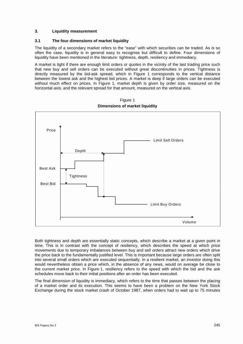
BIS Papers No 2 245
3. Liquidity measurement
3.1 The four dimensions of market liquidity
The liquidity of a secondary market refers to the “ease” with which securities can be traded. As is sooften the case, liquidity is in general easy to recognise but difficult to define. Four dimensions ofliquidity have been mentioned in the literature: tightness, depth, resiliency and immediacy.
A market is tight if there are enough limit orders or quotes in the vicinity of the last trading price suchthat new buy and sell orders can be executed without great discontinuities in prices. Tightness isdirectly measured by the bid-ask spread, which in Figure 1 corresponds to the vertical distancebetween the lowest ask and the highest bid prices. A market is deep if large orders can be executedwithout much effect on prices. In Figure 1, market depth is given by order size, measured on thehorizontal axis, and the relevant spread for that amount, measured on the vertical axis.
Figure 1
Dimensions of market liquidity
Both tightness and depth are essentially static concepts, which describe a market at a given point intime. This is in contrast with the concept of resiliency, which describes the speed at which pricemovements due to temporary imbalances between buy and sell orders attract new orders which drivethe price back to the fundamentally justified level. This is important because large orders are often splitinto several small orders which are executed sequentially. In a resilient market, an investor doing thiswould nevertheless obtain a price which, in the absence of any news, would on average be close tothe current market price. In Figure 1, resiliency refers to the speed with which the bid and the askschedules move back to their initial positions after an order has been executed.
The final dimension of liquidity is immediacy, which refers to the time that passes between the placingof a market order and its execution. This seems to have been a problem on the New York StockExchange during the stock market crash of October 1987, when orders had to wait up to 75 minutes
Tightness
Depth
Price
Volume
Limit Sell Orders
Limit Buy Orders
Best Ask
Best Bid

246 BIS Papers No 2
for execution, apparently due to long printing queues.11 Unfortunately, immediacy cannot be testedwith transactions or quote data, since the time when an order was submitted is not known.
3.2 Measures for market liquidity
Market liquidity has traditionally been proxied by indicators for market activity like the number oftrades, trading volume or the spacing between trades.12 These measures have the advantage thatthey are immediately available or at least easy to compute, but unfortunately are not directly related toany of the four dimensions of liquidity presented in the previous subsection. Market liquidity is onlyone, and not necessarily the most important, factor affecting trading activity. For example, if tradershave sufficiently large hedging needs, then they may trade even if market liquidity, in terms oftightness, depth, resiliency and immediacy, is relatively low.
Nevertheless, even though there is not a one to one relationship between trading activity and liquidity,indicators such as turnover or the intervals between trades do show that markets are sufficiently liquidto sustain a given amount of trading. The converse is not the case, however. The absence oftransactions does not necessarily imply that markets are not liquid but may be due to the agents notwanting to trade at the market clearing prices. Such no-trade equilibria are common in theoreticalmodels with homogenous agents. So, while we should not discard activity indicators altogether, itwould be preferable to have measures that are linked to at least one of the four dimensions of marketliquidity.
A measure for liquidity that is both easily available and in line with one of the four dimensionsmentioned before is the quoted bid-ask spread, which indicates the tightness of a market. In quote-driven markets such as the over-the-counter market for German government bonds quoted spreadscan be observed by traders at any point in time.13 Unfortunately, quoted spreads may not representthe true cost of trading since many transactions take place at prices inside the quoted bid-ask bracket.In addition, they apply to transactions up to a specified amount only, which, furthermore, varies overtime. E.g., if market participants cut this amount in periods of stress, then this would leave the quotedspread unchanged.
We can overcome the problems associated with quoted spreads by computing effective spreads. Incontrast to the former, effective spreads refer to the average transaction and thus captures not onlythe tightness but also the depth of a market. They are computed from transactions data and thusreflect the price actually paid by traders and not the price announced by dealers.
The computation of the effective spread goes back to the seminal work of Roll (1984), who uses thenegative first order autocorrelation in transaction prices that results from transactions beingundertaken alternately at bid and ask prices. Assuming that buy and sell orders arrive with equalprobability and that the bid-ask spread effectively paid by the traders remains constant over theestimation period, he shows that the spread is given by
( )s Cov P Pt t= − −2 1∆ ∆,
Unfortunately, there are a number of problems associated with the Roll measure. First of all, as isshown in Stoll (1989), in the presence of adverse selection or inventory effects it may underestimatethe actual spread. Secondly, a bias may be induced by the fact that the number of bid and offertransactions may not be balanced.14 Nevertheless, its simplicity and the ease with which it is
11Brady (1989).
12For examples, see BIS (1999b).
13Since there is no commitment to market making in the OTC market for Bundesanleihen, quoted spreads are merelyindicative, ie agents do not have to honour the prices they promise. While this should not matter in normal times, it may be aproblem in periods of stress.
14See Choi et al (1988) on how to adjust Roll’s estimator for this.
BIS Papers No 2 247
implemented make the Roll measure a good starting point when measuring liquidity, although itslimitations have to be borne in mind.15
More recently, several other ways for computing spreads from transactions data have beendeveloped.16 Their computation is more involved than that of the Roll measure, which is why they havenot been included in this paper.
4. The market for German government bonds17
This section describes the trading arrangements in the market for German government bonds. As isgenerally the case in the microstructure literature, the institutional structure of a market is of greatimportance since it conditions the availability of data and is important for the interpretation of theresults. A description of the structure of the market for German government securities is also ofinterest in its own right, since it differs from that of other securities markets.
The market for German 10 year Bundesanleihen (Bunds) represents the most liquid segment of theEuropean bond market and provides a benchmark for the pricing of long maturity bonds throughoutEurope. German government bonds are traded both on organised exchanges and over the counter(OTC), with the latter accounting for the bulk of trading. This is especially true for the inter-dealermarket, where trading takes place either directly between banks or through inter-dealer brokers(Freimakler). These act as intermediaries, but have no obligation to provide firm quotes. While theacademic literature would suggest that dealers use brokers mainly in order to obtain anonymity,18
conversations with market participants have hinted at a more mundane reason: Brokers seem to bemore efficient in matching counterparties because of their more active participation in the market.
While there is a trend towards electronic trading, this stage had not yet been reached during 1998,when brokers posted their quotes on screen but the actual transactions took place over the phone.Electronic trading is more important in the client market. Large banks run proprietary trading systems,where they provide quotes for their customers. Recently, electronic trading systems as the Euro-MTShave become more important also in the inter-dealer market, but in 1998 their role was negligible.
The OTC market seems to be rather opaque. Participants observe quotes but do not receive timelyinformation on other traders’ past transactions beyond anecdotal evidence. In principle, it would bepossible to obtain this information from clearing data, but it would arrive with a delay of up to threedays and would be expensive to collect.
The role of exchanges is minor in comparison to the OTC market, even though all issues are listed.Trading takes place almost exclusively on the Frankfurt Stock Exchange, the role of regionalexchanges is negligible. In 1998, German government bonds traded more or less entirely by openoutcry since the computerised trading system XETRA did not permit traders to link their quotes to theprice of the Bund future.19 Prices are formed by a specialist broker (Kursmakler), who has to ensureprice continuity. If the potential market clearing price lies outside a pre-specified corridor, he interruptstrading for five minutes and calls for new quotes. He may undertake some trading on his own account,
15Two practical difficulties may arise when implementing Roll’s method. Firstly, the estimate for Cov ( Pt Pt-1) may benegative. In this case, I drop the observation from the sample. Secondly, the fact that the autocovariance of prices is notknown but has to be estimated from the data induces a small sample bias. This can become a problem when estimating theeffective spread over short time intervals like individual days. However, Roll (1984) argues that the bias is relatively small,eg for a sample of 60 observations it would amount to about two percent of the spread, which would seem acceptable. I dealwith the problem dropping all intervals with less than 50 observations.
16They are surveyed in Huang & Stoll (1997), who also present their own measure for estimating and decomposing thespread into the components due to order-processing, inventory control and adverse selection costs.
17The description of the market for Bunds draws from conversations with Gerhard Klopf and Uwe Ullrich, of the trading desksof the Bundesbank and Deutsche Bank, respectively. I focus the market for Bunds as it was in 1998 and ignore many recentdevelopments.
18At least temporarily, as the banks receive details on their counterparty for clearing purposes. Only very recently did brokersact as a counterparty, thus preserving anonymity even after clearing.
19This possibility has been provided in the summer of 1999, but it remains to be seen whether this will shift more activity ontoXETRA.

248 BIS Papers No 2
but this occurs mainly to offset imbalances in order size and does not seem to play a big role inproviding market liquidity.
5. Data
5.1 Description
The data covers all transactions in Germany during 1998 of four government bonds (Bunds) with aresidual maturity of 8 to 10 years. It includes all Bundesanleihen (long term bonds issued by thefederal government) with an original maturity of 10 years that were issued between January 1997 andJuly 1998. Details on the individual bonds are given in Table 2. The securities have been selectedbecause they were delivered for the Eurex Bund future in 1998.
Bundesanleihen are usually first issued in January and July, and the size of the issue is increasedduring the following months. The autumn of 1998 marked an exception to this rule, as in the wake offalling interest rates a new issue with a lower coupon was brought to the market outside the normalissuing schedule in November. As a consequence, the 4.75% bond first issued in July 1998 has avolume outstanding of only 17 billion DM compared to 30 billion DM for the other three bonds in oursample.
The data has been provided by the German securities’ regulator Bundesaufsichtsamt für denWertpapierhandel (BAWe), which receives notice of every single transaction in Germany, irrespectiveof whether or not it takes place on an exchange. This feature is particularly attractive for work on thebond market, where OTC transactions account for most trading.
Bunds are also traded abroad, in particular in London. Unfortunately, we do not have any informationon transactions outside Germany, although there is anecdotal evidence that the market share ofLondon has fallen in recent years, albeit by a lesser extent than the one in the market for Bundfutures.
In principle, we should have two observations for each trade: one concerning the final buyer andanother for the final seller of the security. An exception are trades with intermediaries that resideoutside Germany and are therefore not subject to the reporting requirement. For each observation, wehave a date and time stamp, price, volume, as well as indicators for whether it is the sale or thepurchase leg of a transaction, whether the reporting bank’s inventory is affected, whether the reportingbank acts as an agent for a customer or on its own account, and whether trade takes place over thecounter or on an exchange.
Some observations on the quality of the data are in order. Firstly, the precision of the time stamps (upto the nearest second) may be more apparent than real. It is probably high for trades that take placeon an exchange, but may be low for OTC-transactions. An indication for this is that many trades arereported as taking place outside normal office hours, often at midnight sharp or at prices that seem outof date. Inaccurate time stamps represent a severe problem since the reliability of most indicators forliquidity crucially depend on the correct sequence, although not so much the timing, of trades.Secondly, other variables may have been reported incorrectly. While most of such errors have beeneliminated by the BAWe using supplementary information, some mistakes especially in prices orvolume may remain.
Matching the buy and sell legs of transactions and filtering the data can reduce the severeness ofthese problems. Unfortunately, matching the two legs is not straightforward, in part because of errorsin the data and in part because of missing notifications. I have matched all purchases and sales thatoccurred on the same day at the same price and with the same volume. If the time stamps of thesepairs of “matched” observations do not coincide, I have used the earlier one. Of a total of 145thousand observations in our raw data, only about half could be matched in this way.20 Since theremaining “unmatched” observations account for a large proportion of market activity, I have decidedto keep them in the data. After matching, we are left with 109 thousand observations, which further
20The BAWe successfully matches the various notices for more than three quarters of the trades but uses supplemental datato achieve this. They use the matches in order to hunt down missing notifications and to eliminate contra-trades. Since thematches are stored in a different database, using this information in the present study would have incurred computationalcosts that seemed out of proportion to the limited benefits of doing so.
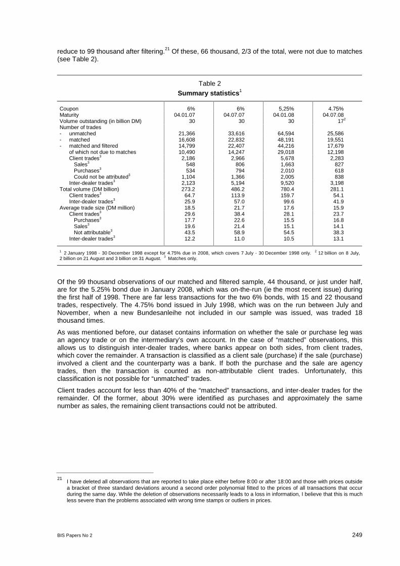
BIS Papers No 2 249
reduce to 99 thousand after filtering.21 Of these, 66 thousand, 2/3 of the total, were not due to matches(see Table 2).
Table 2
Summary statistics1
Coupon 6% 6% 5,25% 4.75%Maturity 04.01.07 04.07.07 04.01.08 04.07.08Volume outstanding (in billion DM) 30 30 30 172
Number of trades- unmatched 21,366 33,616 64,594 25,586- matched 16,608 22,832 48,191 19,551- matched and filtered 14,799 22,407 44,216 17,679
of which not due to matches 10,490 14,247 29,018 12,198Client trades3 2,186 2,966 5,678 2,283
Sales3 548 806 1,663 827Purchases3 534 794 2,010 618Could not be attributed3 1,104 1,366 2,005 838
Inter-dealer trades3 2,123 5,194 9,520 3,198Total volume (DM billion) 273.2 486.2 780.4 281.1
Client trades3 64.7 113.9 159.7 54.1Inter-dealer trades3 25.9 57.0 99.6 41.9
Average trade size (DM million) 18.5 21.7 17.6 15.9Client trades3 29.6 38.4 28.1 23.7
Purchases3 17.7 22.6 15.5 16.8Sales3 19.6 21.4 15.1 14.1Not attributable3 43.5 58.9 54.5 38.3
Inter-dealer trades3 12.2 11.0 10.5 13.1
1 2 January 1998 - 30 December 1998 except for 4.75% due in 2008, which covers 7 July - 30 December 1998 only. 2 12 billion on 8 July,2 billion on 21 August and 3 billion on 31 August. 3 Matches only.
Of the 99 thousand observations of our matched and filtered sample, 44 thousand, or just under half,are for the 5.25% bond due in January 2008, which was on-the-run (ie the most recent issue) duringthe first half of 1998. There are far less transactions for the two 6% bonds, with 15 and 22 thousandtrades, respectively. The 4.75% bond issued in July 1998, which was on the run between July andNovember, when a new Bundesanleihe not included in our sample was issued, was traded 18thousand times.
As was mentioned before, our dataset contains information on whether the sale or purchase leg wasan agency trade or on the intermediary’s own account. In the case of “matched” observations, thisallows us to distinguish inter-dealer trades, where banks appear on both sides, from client trades,which cover the remainder. A transaction is classified as a client sale (purchase) if the sale (purchase)involved a client and the counterparty was a bank. If both the purchase and the sale are agencytrades, then the transaction is counted as non-attributable client trades. Unfortunately, thisclassification is not possible for “unmatched” trades.
Client trades account for less than 40% of the “matched” transactions, and inter-dealer trades for theremainder. Of the former, about 30% were identified as purchases and approximately the samenumber as sales, the remaining client transactions could not be attributed.
21I have deleted all observations that are reported to take place either before 8:00 or after 18:00 and those with prices outsidea bracket of three standard deviations around a second order polynomial fitted to the prices of all transactions that occurduring the same day. While the deletion of observations necessarily leads to a loss in information, I believe that this is muchless severe than the problems associated with wrong time stamps or outliers in prices.
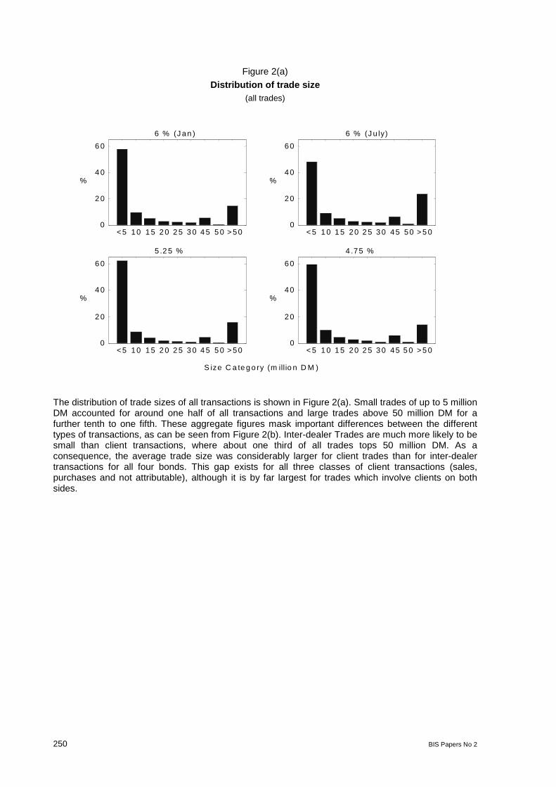
250 BIS Papers No 2
Figure 2(a)Distribution of trade size
(all trades)
<5 10 1 5 2 0 2 5 3 0 4 5 5 0 > 500
2 0
4 0
6 0
6 % (J an )
%
< 5 1 0 1 5 20 2 5 3 0 45 50 > 5 00
20
40
60
6 % (J u ly)
%
<5 10 1 5 2 0 2 5 3 0 4 5 5 0 > 500
2 0
4 0
6 0
5 .2 5 %
%
< 5 1 0 1 5 20 2 5 3 0 45 5 0 > 5 00
20
40
60
4 .75 %
%
S ize C a te g o ry (m illio n D M )
The distribution of trade sizes of all transactions is shown in Figure 2(a). Small trades of up to 5 millionDM accounted for around one half of all transactions and large trades above 50 million DM for afurther tenth to one fifth. These aggregate figures mask important differences between the differenttypes of transactions, as can be seen from Figure 2(b). Inter-dealer Trades are much more likely to besmall than client transactions, where about one third of all trades tops 50 million DM. As aconsequence, the average trade size was considerably larger for client trades than for inter-dealertransactions for all four bonds. This gap exists for all three classes of client transactions (sales,purchases and not attributable), although it is by far largest for trades which involve clients on bothsides.

BIS Papers No 2 251
Figure 2(b)Distribution of trade size
(client and inter-dealer trades)
< 5 1 0 1 5 2 0 2 5 3 0 4 5 5 0 > 5 00
2 0
4 0
6 0
8 06 % (J a n )
%
C lie n tsB a n k s
< 5 1 0 1 5 2 0 2 5 3 0 4 5 5 0 > 5 00
2 0
4 0
6 0
8 06 % (J u ly )
%
C lie n tsB a n k s
< 5 1 0 1 5 2 0 2 5 3 0 4 5 5 0 > 5 00
2 0
4 0
6 0
8 05 .2 5 %
%
C lie n tsB a n k s
< 5 1 0 1 5 2 0 2 5 3 0 4 5 5 0 > 5 00
2 0
4 0
6 0
8 04 .7 5 %
%
S iz e C a te g o r y (m il l io n D M )
C lie n tsB a n k s
Our data also contains information on whether or not a trade affected the reporting bank’s inventory,which permits us to construct a series for the aggregate inventory of the banking sector at any givenpoint in time by simply adding up all transactions which affect inventories, and assuming that theinventory at the beginning of the year was zero. In the case of the two 6% bonds, this latterassumption is arbitrary, the inventory series for these bonds can therefore only be interpreted in termsof movement over time but not in terms of the actual level of inventory.
Figure 3 shows the inventories at the end of each trading day for the four bonds.22 They tend tofluctuate within a relatively narrow band around zero. On more than 50% of all days, they are between–10 and +10 million DM, which is considerably less than the average transaction size, and exceed 100million or are below –100 million on only 5% of trading days.
According to our figures, between 78% and 86% of all trades took place over the counter,23 althoughthis may understate the true figure as many OTC-transactions after execution are entered into anexchange’s trading system in order to take advantage of the automated clearing facilities, andreporting banks may “forget” to enter the variable correctly.
22End-of-day inventories have been computed from the unfiltered data, since dropping any transaction would reduce thereliability of the data. In addition, misreported time stamps or prices do not have any effects on the quality of the series.
23Trades are counted as OTC if identified by the börslich-flag or if recorded before 8:00 or after 18:00 hours.

252 BIS Papers No 2
Figure 3End-of-day inventories
1 2 3 4 5 6 7 8 9 10 11 12
-200
-100
0
100
200
3006% (January)
1 2 3 4 5 6 7 8 9 10 11 12
-200
-100
0
100
200
3006% (Jul)
1 2 3 4 5 6 7 8 9 10 11 12
-200
-100
0
100
200
3005.25%
Month 1 2 3 4 5 6 7 8 9 10 11 12
-200
-100
0
100
200
3004.75%
Month
In m illion DM
5.2 Intra-day patterns of trading activity
Trading activity is very unevenly distributed over the trading day, as can be seen from figures 4(a) –(c), which plot the distribution of the number of trades, turnover and average trade sizes within halfhourly intervals. Trading activity shows two peaks during the day. The first peak occurs in the morningbetween 9:30 to 10:00, when around 10% of all trades take place, which however account for a muchhigher share of daily turnover. The average trade size in this half hour period is consequently morethan twice as high as during the remainder of the day. The second peak in activity occurs between11:30 and 12:00, when between 12% to more than 20% of all trades take place. These tend to besmall trades, however, with an average trade size below that of any other interval. Trading is leastheavy in the early morning, before 8:30, at lunchtime between 13:00 to 14:00, and in the evening after17:00.
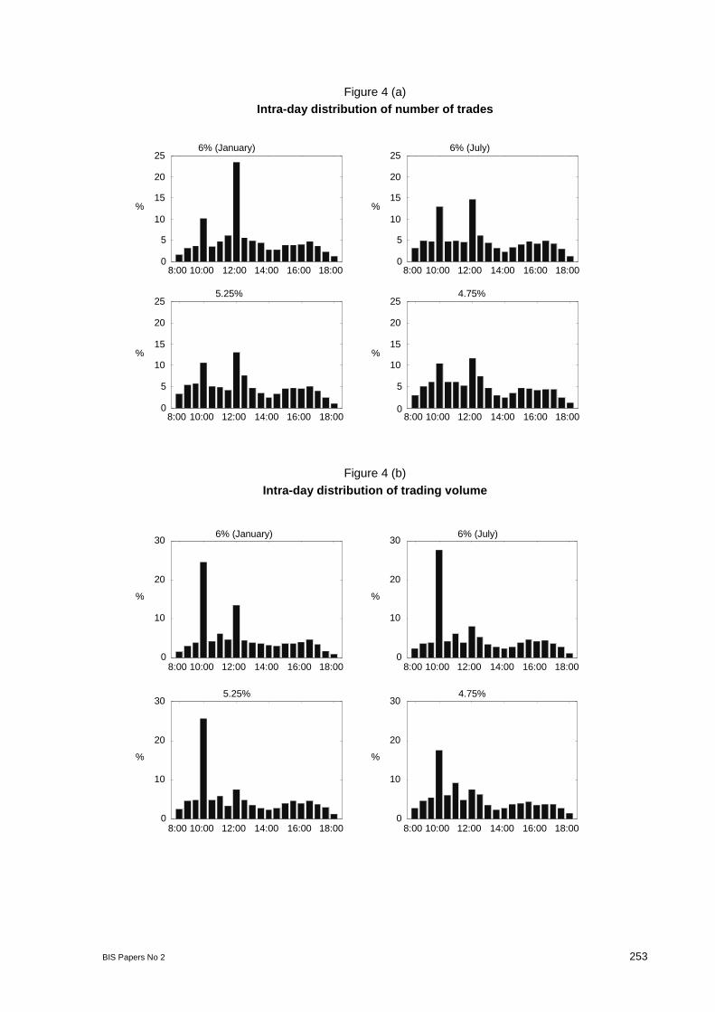
BIS Papers No 2 253
Figure 4 (a)Intra-day distribution of number of trades
8:00 10:00 12:00 14:00 16:00 18:000
5
10
15
20
25
%
6% (January)
8:00 10:00 12:00 14:00 16:00 18:000
5
10
15
20
25
%
6% (July)
8:00 10:00 12:00 14:00 16:00 18:000
5
10
15
20
25
%
5.25%
8:00 10:00 12:00 14:00 16:00 18:000
5
10
15
20
25
%
4.75%
Figure 4 (b)
Intra-day distribution of trading volume
8:00 10:00 12:00 14:00 16:00 18:000
10
20
30
%
6% (January)
8:00 10:00 12:00 14:00 16:00 18:000
10
20
30
%
6% (July)
8:00 10:00 12:00 14:00 16:00 18:000
10
20
30
%
5.25%
8:00 10:00 12:00 14:00 16:00 18:000
10
20
30
%
4.75%
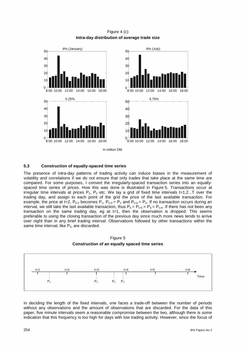
254 BIS Papers No 2
Figure 4 (c)Intra-day distribution of average trade size
8:00 10:00 12:00 14:00 16:00 18:000
10
20
30
40
506% (January)
8:00 10:00 12:00 14:00 16:00 18:000
10
20
30
40
506% (July)
8:00 10:00 12:00 14:00 16:00 18:000
10
20
30
40
505.25%
8:00 10:00 12:00 14:00 16:00 18:000
10
20
30
40
504.75%
In million DM
5.3 Construction of equally-spaced time series
The presence of intra-day patterns of trading activity can induce biases in the measurement ofvolatility and correlations if we do not ensure that only trades that take place at the same time arecompared. For some purposes, I convert the irregularly-spaced transaction series into an equally-spaced time series of prices. How this was done is illustrated in Figure 5. Transactions occur atirregular time intervals at prices P1, P2 etc. We lay a grid of fixed time intervals t=1,2...T over thetrading day, and assign to each point of the grid the price of the last available transaction. Forexample, the price at t=2, Pt=2 becomes P1, Pt=3 = P2 and Pt=4 = P4. If no transaction occurs during aninterval, we still take the last available transaction, thus P5 = Pt=5 = P4 = Pt=4. If there has not been anytransaction on the same trading day, eg at t=1, then the observation is dropped. This seemspreferable to using the closing transaction of the previous day since much more news tends to arriveover night than in any brief trading interval. Observations followed by other transactions within thesame time interval, like P3, are discarded.
Figure 5
Construction of an equally spaced time series
In deciding the length of the fixed intervals, one faces a trade-off between the number of periodswithout any observations and the amount of observations that are discarded. For the data of thispaper, five minute intervals seem a reasonable compromise between the two, although there is someindication that this frequency is too high for days with low trading activity. However, since the focus of
Time
t=1 t=2 t=3 t=4 t=5 t=6
P1 P2 P3 P4
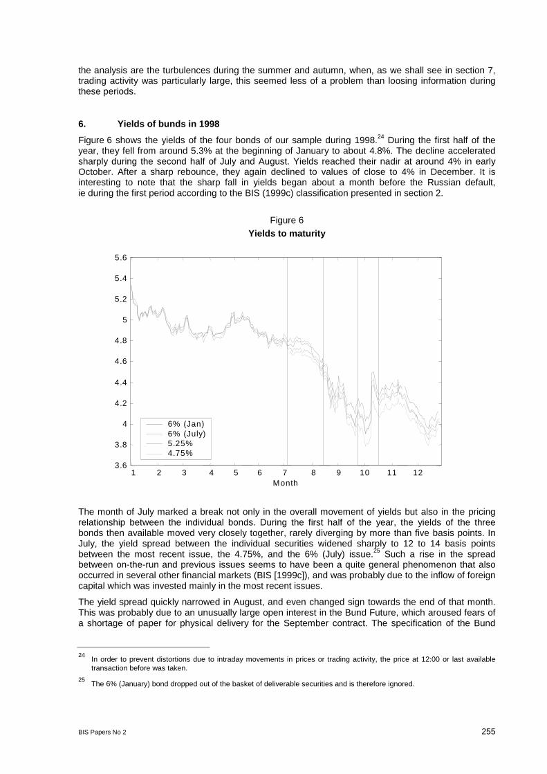
BIS Papers No 2 255
the analysis are the turbulences during the summer and autumn, when, as we shall see in section 7,trading activity was particularly large, this seemed less of a problem than loosing information duringthese periods.
6. Yields of bunds in 1998
Figure 6 shows the yields of the four bonds of our sample during 1998.24 During the first half of theyear, they fell from around 5.3% at the beginning of January to about 4.8%. The decline acceleratedsharply during the second half of July and August. Yields reached their nadir at around 4% in earlyOctober. After a sharp rebounce, they again declined to values of close to 4% in December. It isinteresting to note that the sharp fall in yields began about a month before the Russian default,ie during the first period according to the BIS (1999c) classification presented in section 2.
Figure 6
Yields to maturity
1 2 3 4 5 6 7 8 9 10 11 123.6
3.8
4
4.2
4.4
4.6
4.8
5
5.2
5.4
5.6
Month
6% (Jan)6% (July)5.25%4.75%
The month of July marked a break not only in the overall movement of yields but also in the pricingrelationship between the individual bonds. During the first half of the year, the yields of the threebonds then available moved very closely together, rarely diverging by more than five basis points. InJuly, the yield spread between the individual securities widened sharply to 12 to 14 basis pointsbetween the most recent issue, the 4.75%, and the 6% (July) issue.25 Such a rise in the spreadbetween on-the-run and previous issues seems to have been a quite general phenomenon that alsooccurred in several other financial markets (BIS [1999c]), and was probably due to the inflow of foreigncapital which was invested mainly in the most recent issues.
The yield spread quickly narrowed in August, and even changed sign towards the end of that month.This was probably due to an unusually large open interest in the Bund Future, which aroused fears ofa shortage of paper for physical delivery for the September contract. The specification of the Bund
24In order to prevent distortions due to intraday movements in prices or trading activity, the price at 12:00 or last availabletransaction before was taken.
25The 6% (January) bond dropped out of the basket of deliverable securities and is therefore ignored.
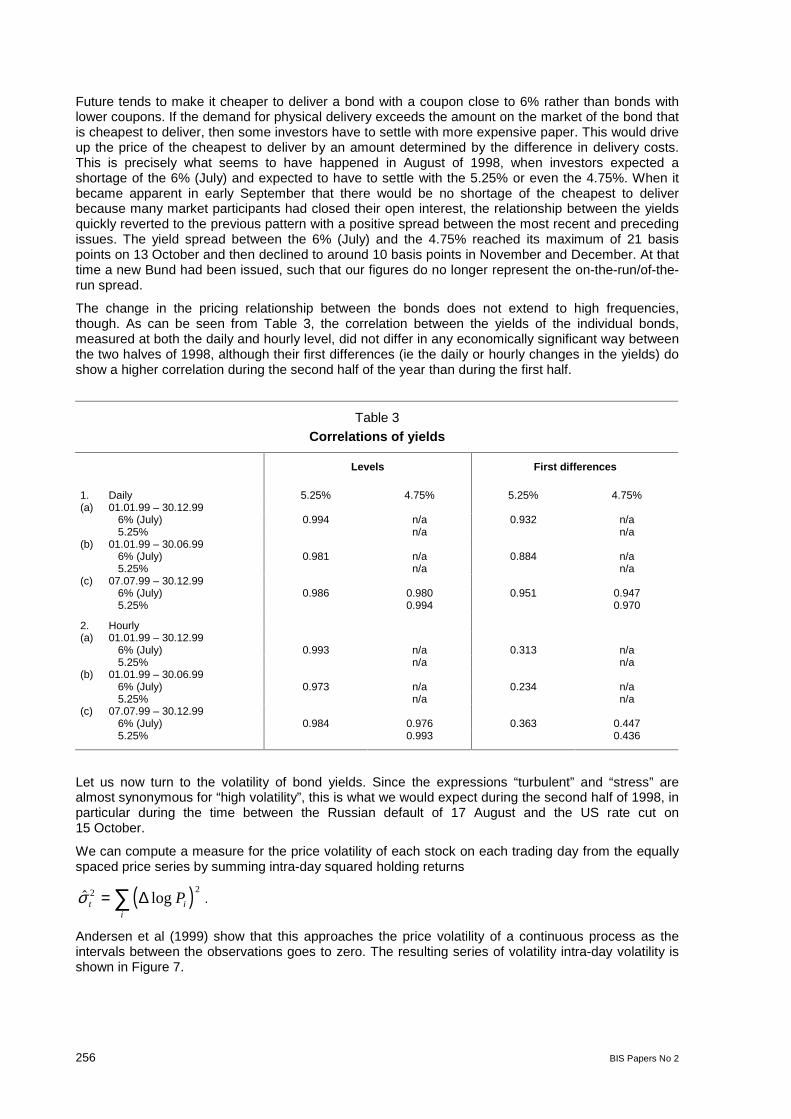
256 BIS Papers No 2
Future tends to make it cheaper to deliver a bond with a coupon close to 6% rather than bonds withlower coupons. If the demand for physical delivery exceeds the amount on the market of the bond thatis cheapest to deliver, then some investors have to settle with more expensive paper. This would driveup the price of the cheapest to deliver by an amount determined by the difference in delivery costs.This is precisely what seems to have happened in August of 1998, when investors expected ashortage of the 6% (July) and expected to have to settle with the 5.25% or even the 4.75%. When itbecame apparent in early September that there would be no shortage of the cheapest to deliverbecause many market participants had closed their open interest, the relationship between the yieldsquickly reverted to the previous pattern with a positive spread between the most recent and precedingissues. The yield spread between the 6% (July) and the 4.75% reached its maximum of 21 basispoints on 13 October and then declined to around 10 basis points in November and December. At thattime a new Bund had been issued, such that our figures do no longer represent the on-the-run/of-the-run spread.
The change in the pricing relationship between the bonds does not extend to high frequencies,though. As can be seen from Table 3, the correlation between the yields of the individual bonds,measured at both the daily and hourly level, did not differ in any economically significant way betweenthe two halves of 1998, although their first differences (ie the daily or hourly changes in the yields) doshow a higher correlation during the second half of the year than during the first half.
Table 3Correlations of yields
Levels First differences
1. Daily 5.25% 4.75% 5.25% 4.75%(a) 01.01.99 – 30.12.99
6% (July) 0.994 n/a 0.932 n/a5.25% n/a n/a
(b) 01.01.99 – 30.06.996% (July) 0.981 n/a 0.884 n/a5.25% n/a n/a
(c) 07.07.99 – 30.12.996% (July) 0.986 0.980 0.951 0.9475.25% 0.994 0.970
2. Hourly(a) 01.01.99 – 30.12.99
6% (July) 0.993 n/a 0.313 n/a5.25% n/a n/a
(b) 01.01.99 – 30.06.996% (July) 0.973 n/a 0.234 n/a5.25% n/a n/a
(c) 07.07.99 – 30.12.996% (July) 0.984 0.976 0.363 0.4475.25% 0.993 0.436
Let us now turn to the volatility of bond yields. Since the expressions “turbulent” and “stress” arealmost synonymous for “high volatility”, this is what we would expect during the second half of 1998, inparticular during the time between the Russian default of 17 August and the US rate cut on15 October.
We can compute a measure for the price volatility of each stock on each trading day from the equallyspaced price series by summing intra-day squared holding returns
( ) logσ t ii
P2 2= ∑ ∆ .
Andersen et al (1999) show that this approaches the price volatility of a continuous process as theintervals between the observations goes to zero. The resulting series of volatility intra-day volatility isshown in Figure 7.
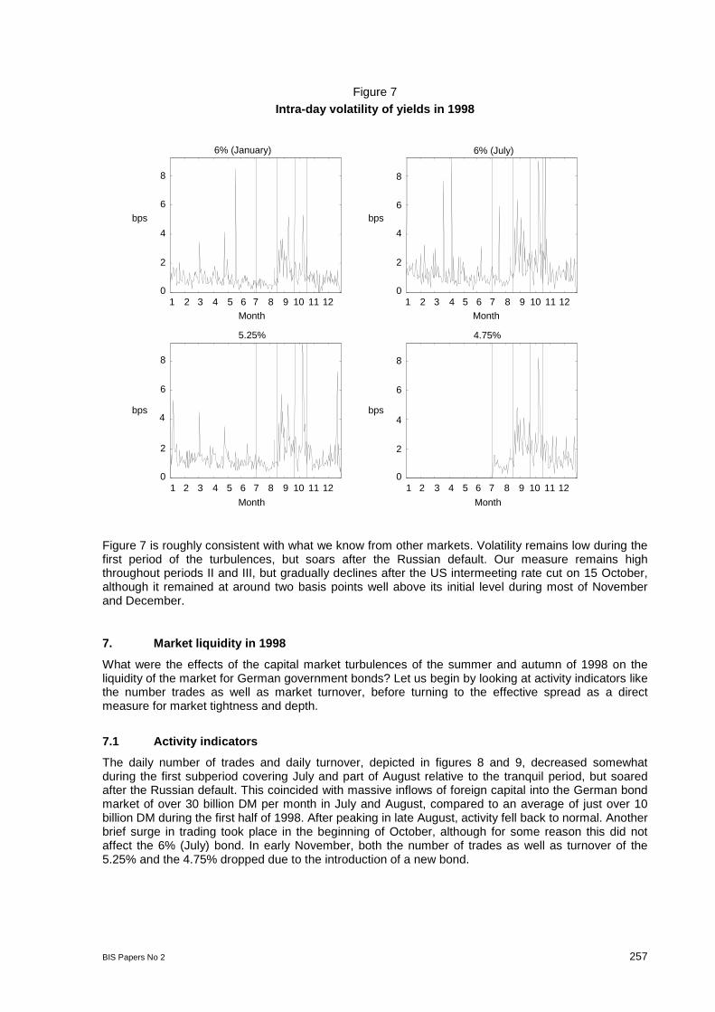
BIS Papers No 2 257
Figure 7Intra-day volatility of yields in 1998
1 2 3 4 5 6 7 8 9 10 11 120
2
4
6
8
6% (January)
Month 1 2 3 4 5 6 7 8 9 10 11 12
0
2
4
6
8
6% (July)
Month
1 2 3 4 5 6 7 8 9 10 11 120
2
4
6
8
5.25%
Month
1 2 3 4 5 6 7 8 9 10 11 120
2
4
6
8
4.75%
Month
bps bps
bps bps
Figure 7 is roughly consistent with what we know from other markets. Volatility remains low during thefirst period of the turbulences, but soars after the Russian default. Our measure remains highthroughout periods II and III, but gradually declines after the US intermeeting rate cut on 15 October,although it remained at around two basis points well above its initial level during most of Novemberand December.
7. Market liquidity in 1998
What were the effects of the capital market turbulences of the summer and autumn of 1998 on theliquidity of the market for German government bonds? Let us begin by looking at activity indicators likethe number trades as well as market turnover, before turning to the effective spread as a directmeasure for market tightness and depth.
7.1 Activity indicators
The daily number of trades and daily turnover, depicted in figures 8 and 9, decreased somewhatduring the first subperiod covering July and part of August relative to the tranquil period, but soaredafter the Russian default. This coincided with massive inflows of foreign capital into the German bondmarket of over 30 billion DM per month in July and August, compared to an average of just over 10billion DM during the first half of 1998. After peaking in late August, activity fell back to normal. Anotherbrief surge in trading took place in the beginning of October, although for some reason this did notaffect the 6% (July) bond. In early November, both the number of trades as well as turnover of the5.25% and the 4.75% dropped due to the introduction of a new bond.
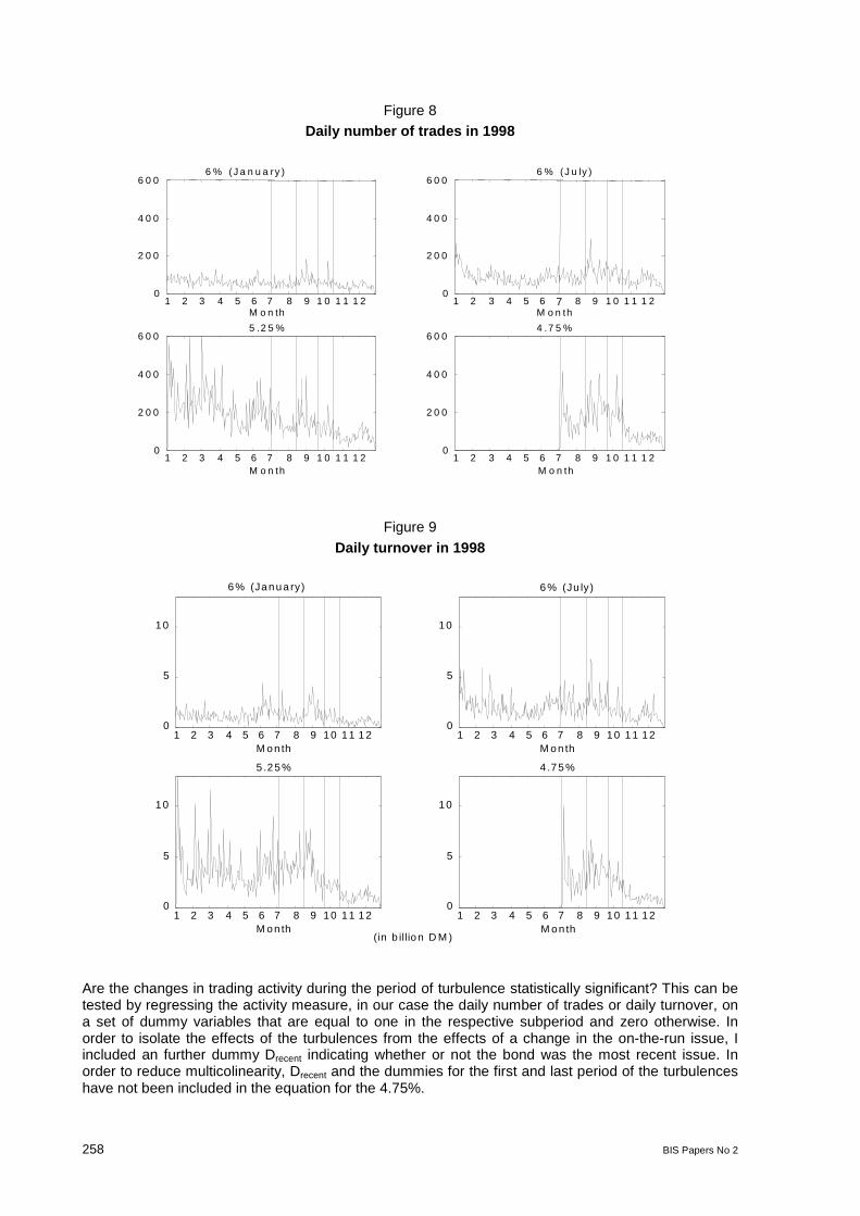
258 BIS Papers No 2
Figure 8Daily number of trades in 1998
1 2 3 4 5 6 7 8 9 1 0 1 1 1 20
2 0 0
4 0 0
6 0 06 % (J a n u a ry )
M o n th 1 2 3 4 5 6 7 8 9 1 0 1 1 1 2
0
2 0 0
4 0 0
6 0 06 % (J u ly )
M o n th
1 2 3 4 5 6 7 8 9 1 0 1 1 1 20
2 0 0
4 0 0
6 0 05 .2 5 %
M o n th 1 2 3 4 5 6 7 8 9 1 0 1 1 1 2
0
2 0 0
4 0 0
6 0 04 .7 5 %
M o n th
Figure 9
Daily turnover in 1998
1 2 3 4 5 6 7 8 9 10 11 120
5
10
6% (Janua ry)
M on th 1 2 3 4 5 6 7 8 9 10 11 12
0
5
10
6% (Ju ly)
M on th
1 2 3 4 5 6 7 8 9 10 11 120
5
10
5 .25%
M on th 1 2 3 4 5 6 7 8 9 10 11 12
0
5
10
4 .75%
M on th(in b illion D M )
Are the changes in trading activity during the period of turbulence statistically significant? This can betested by regressing the activity measure, in our case the daily number of trades or daily turnover, ona set of dummy variables that are equal to one in the respective subperiod and zero otherwise. Inorder to isolate the effects of the turbulences from the effects of a change in the on-the-run issue, Iincluded an further dummy Drecent indicating whether or not the bond was the most recent issue. Inorder to reduce multicolinearity, Drecent and the dummies for the first and last period of the turbulenceshave not been included in the equation for the 4.75%.

BIS Papers No 2 259
Table 4Trading activity during the 1998 turbulences
6% (Jan.) 6% (July) 5.25% 4.75%
Dep. variable (i) (ii) (i) (ii) (i) (ii) (i) (ii)
Expl. variablesD6.7.-14.8. -0.00
(-0.01)**-0.29(-1.85)
***0.38(3.47)
**0.29(2.04)
0.16(0.33)
0.52(0.94)
- -
D17.8.-22-9. ***0.61(4.84)
**0.35(1.87)
***1.09(8.37)
***0.75(4.48)
0.46(0.91)
0.48(0.83)
***0.93(8.45)
***0.94(6.65)
D23.9.-15.10. ***0.46(3.05)
*-0.333(-1.46)
***0.96(6.08)
*0.29(1.38)
0.37(0.73)
0.05(0.09)
***0.68(5.12)
***0.50(2.94)
D16.10.-31.12. 0.07(0.42)
***-0.92(-3.83)
***0.69(4.13)
0.07(0.30)
0.28(0.54)
-0.22(-0.37)
- -
Drecent - - 0.25(0.63)
0.15(0.28)
0.16(0.33)
0.11(0.20)
- -
# observations 250 250 250 250 249 249 124 124
Dependent variable: (i) daily number of trades, (ii) daily turnover, normalised by their mean. T-values in brackets. Dummies equal to 1 duringindicated period and zero otherwise, dummy recent one if on-the-run and zero otherwise. Explanatory variables also include a constant and timetrend. Newey-West correction for autocorrelation and heteroscedasticity. Significant on *90%, **95%, ***99% confidence level
The results of the regressions are displayed in Table 4. They indicate that the surge in both thenumber of trades and in turnover during the second period of the turbulences is statistically highlysignificant. The only exception to this is the 5.25% bond, where none of the dummies, including ,Drecent, proved to be significant. There is also some indication that the number of trades, although notin all cases turnover, was higher during the third period than on average. The individual bondsbehaved quite differently during the initial and final periods of the turbulences, when some of thembecame more actively traded and the others less so.
The results indicate that markets have been sufficiently liquid to sustain a larger than normal numberof trades and turnover, but this does not necessarily imply that market liquidity remained unaffected. Itis therefore necessary to look at direct indicator for market liquidity and not solely rely on activityindicators like the number of trades of turnover.
7.2 Effective spreads
Let us now turn to a measure of liquidity that is directly related to both the tightness and the depth ofthe market, the effective spread measured by Roll’s statistic. Before proceeding, a word of caution isneeded. The Roll measure is likely to underestimates the “true” spread in the presence of inventorycontrol or adverse selection effects. Since these are more likely to occur in times of market stress(when prices are more volatile, adding to inventory costs, and there is more scope for privateinformation), our results are liable to underestimate any worsening in market liquidity.
Table 5 shows the Roll measures for the effective spread estimated from transactions prices. Thespreads appear to have been very low, and consequently the market very liquid, during the firstsubperiod of the turbulences ranging from the beginning of July to the eve of the Russian default amonth and half later. After the Russian default, effective spreads increase to 1.73 to 1.9 basis points,although they remain below their level of the first half of the year for the two 6% bonds. They risefurther after the LTCM rescue, to more than 2 basis points. The only exception is the 6% (January)bond, whose effective spread declines to 1.3 basis points. The spreads ease during the fourth andfinal subperiod to levels near or even below that of the first half of the year. It is possible that the oddresult of a very high spread for this bond during the period of tranquillity is due to data problems.
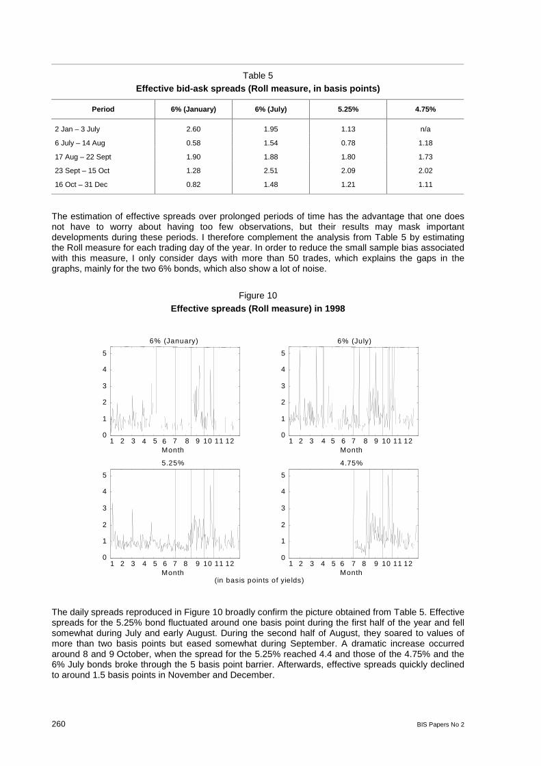
260 BIS Papers No 2
Table 5Effective bid-ask spreads (Roll measure, in basis points)
Period 6% (January) 6% (July) 5.25% 4.75%
2 Jan – 3 July 2.60 1.95 1.13 n/a
6 July – 14 Aug 0.58 1.54 0.78 1.18
17 Aug – 22 Sept 1.90 1.88 1.80 1.73
23 Sept – 15 Oct 1.28 2.51 2.09 2.02
16 Oct – 31 Dec 0.82 1.48 1.21 1.11
The estimation of effective spreads over prolonged periods of time has the advantage that one doesnot have to worry about having too few observations, but their results may mask importantdevelopments during these periods. I therefore complement the analysis from Table 5 by estimatingthe Roll measure for each trading day of the year. In order to reduce the small sample bias associatedwith this measure, I only consider days with more than 50 trades, which explains the gaps in thegraphs, mainly for the two 6% bonds, which also show a lot of noise.
Figure 10
Effective spreads (Roll measure) in 1998
1 2 3 4 5 6 7 8 9 10 11 120
1
2
3
4
5
6% (January)
Month1 2 3 4 5 6 7 8 9 10 11 12
0
1
2
3
4
5
6% (July)
Month
1 2 3 4 5 6 7 8 9 10 11 120
1
2
3
4
5
5.25%
Month1 2 3 4 5 6 7 8 9 10 11 12
0
1
2
3
4
5
4.75%
Month(in basis points of yields)
The daily spreads reproduced in Figure 10 broadly confirm the picture obtained from Table 5. Effectivespreads for the 5.25% bond fluctuated around one basis point during the first half of the year and fellsomewhat during July and early August. During the second half of August, they soared to values ofmore than two basis points but eased somewhat during September. A dramatic increase occurredaround 8 and 9 October, when the spread for the 5.25% reached 4.4 and those of the 4.75% and the6% July bonds broke through the 5 basis point barrier. Afterwards, effective spreads quickly declinedto around 1.5 basis points in November and December.
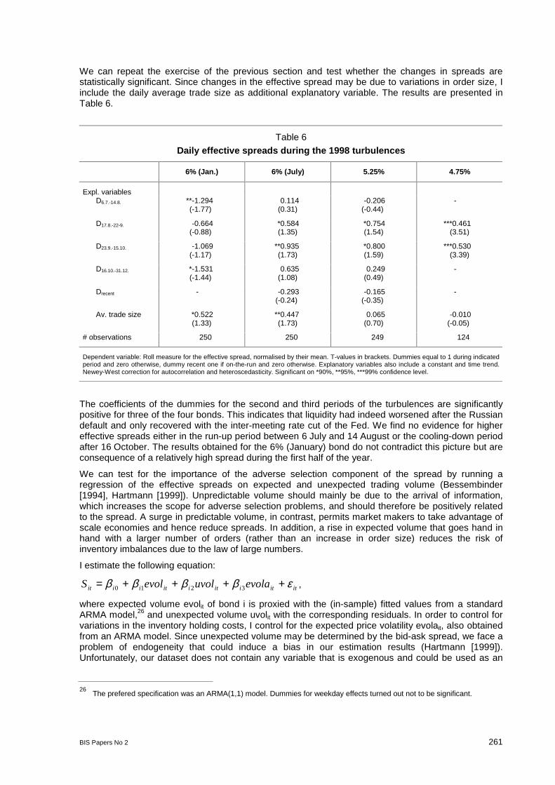
BIS Papers No 2 261
We can repeat the exercise of the previous section and test whether the changes in spreads arestatistically significant. Since changes in the effective spread may be due to variations in order size, Iinclude the daily average trade size as additional explanatory variable. The results are presented inTable 6.
Table 6
Daily effective spreads during the 1998 turbulences
6% (Jan.) 6% (July) 5.25% 4.75%
Expl. variablesD6.7.-14.8. **-1.294
(-1.77)0.114
(0.31)-0.206
(-0.44)-
D17.8.-22-9. -0.664(-0.88)
*0.584(1.35)
*0.754(1.54)
***0.461(3.51)
D23.9.-15.10. -1.069(-1.17)
**0.935(1.73)
*0.800(1.59)
***0.530(3.39)
D16.10.-31.12. *-1.531(-1.44)
0.635(1.08)
0.249(0.49)
-
Drecent - -0.293(-0.24)
-0.165(-0.35)
-
Av. trade size *0.522(1.33)
**0.447(1.73)
0.065(0.70)
-0.010(-0.05)
# observations 250 250 249 124
Dependent variable: Roll measure for the effective spread, normalised by their mean. T-values in brackets. Dummies equal to 1 during indicatedperiod and zero otherwise, dummy recent one if on-the-run and zero otherwise. Explanatory variables also include a constant and time trend.Newey-West correction for autocorrelation and heteroscedasticity. Significant on *90%, **95%, ***99% confidence level.
The coefficients of the dummies for the second and third periods of the turbulences are significantlypositive for three of the four bonds. This indicates that liquidity had indeed worsened after the Russiandefault and only recovered with the inter-meeting rate cut of the Fed. We find no evidence for highereffective spreads either in the run-up period between 6 July and 14 August or the cooling-down periodafter 16 October. The results obtained for the 6% (January) bond do not contradict this picture but areconsequence of a relatively high spread during the first half of the year.
We can test for the importance of the adverse selection component of the spread by running aregression of the effective spreads on expected and unexpected trading volume (Bessembinder[1994], Hartmann [1999]). Unpredictable volume should mainly be due to the arrival of information,which increases the scope for adverse selection problems, and should therefore be positively relatedto the spread. A surge in predictable volume, in contrast, permits market makers to take advantage ofscale economies and hence reduce spreads. In addition, a rise in expected volume that goes hand inhand with a larger number of orders (rather than an increase in order size) reduces the risk ofinventory imbalances due to the law of large numbers.
I estimate the following equation:
ititiitiitiiit evolauvolevolS εββββ ++++= 3210 ,
where expected volume evolit of bond i is proxied with the (in-sample) fitted values from a standardARMA model,26 and unexpected volume uvolit with the corresponding residuals. In order to control forvariations in the inventory holding costs, I control for the expected price volatility evolait, also obtainedfrom an ARMA model. Since unexpected volume may be determined by the bid-ask spread, we face aproblem of endogeneity that could induce a bias in our estimation results (Hartmann [1999]).Unfortunately, our dataset does not contain any variable that is exogenous and could be used as an
26The prefered specification was an ARMA(1,1) model. Dummies for weekday effects turned out not to be significant.
262 BIS Papers No 2
instrument for uvolit.27 We therefore have to live with the endogeneity problem, although we have to
interpret the results in light of the possible bias. The results of the estimation are displayed in Table 7.
Table 7
Effective spreads and trading volume
6% (July) 5.25% 4.75%
Expl. VariablesExp. volume 0.202
(0.87)*0.164(1.89)
0.103(0.92)
Unexp. volume 0.201(0.52)
***0.524(3.72)
***0.659(4.12)
Exp. volatility **0.349(2.44)
***0.555(7.78)
***0.337(4.36)
R2 0.06 0.46 0.25
# observations 124 137 109
F-Test: H0: β1=β2 - **5.4 ***11.4
Sample: 27 May - 30 December, 1998, except for the 4.75%, which started on 6 July. Dependent variable: Roll measure for the effective spread,normalised by their mean. T-values in brackets. Volume: Total volume of all deliverable bonds. Expected Volume: 1-step out-of-sampleforecasts from ARMA-model. Unexpected Volume=Volume-Expected Volume. Explanatory variables also include a constant. Newey-Westcorrection for autocorrelation and heteroscedasticity. Significant on *90%, **95%, ***99% confidence level.
The relationship between unexpected volume and effective spreads is positive and highly significantfor the 5.25% and the 4.75% bonds, which is in line with our hypothesis. The fact that the relevantcoefficient is not significant for the 6% (July) bond may be due to the inordinate amount of noise in theseries for the spread. The coefficients on expected volume are positive, but either insignificant or onlyweakly significant, which indicates that there do not seem to be much economies to scale in marketmaking. The importance of inventory holding costs is shown by the highly significant and positivecoefficient for expected volatility. We can reject the hypothesis that the coefficients of our two volumemeasures are equal for two of the bonds, which is in accordance with the results obtained for the forexmarket (see Hartmann [1999] and references therein).
27Hartmann (1999) uses the quoting (tick) frequency on the Reuters FXFX page. Such quote information is not available to us,since our data only contains information on transactions.
BIS Papers No 2 263
Figure 11Unexpected volume and effective spreads
1 2 3 4 5 6 7 8 9 10 11 12
0
2
4
6
Month
bps
5.25 %
1 2 3 4 5 6 7 8 9 10 11 12
0
2
4
6
Month
bps
4.75 %
Effective spread
Explained by unexpected volume
The strong statistical relationship between unexpected volume and bid-ask spreads cannot explain therise in the latter that occured from August to October. Figure 11 plots the spreads and the proportionthat can be explained by unexpected volume ( i2uvolit). Spreads seem to be related to surprises involume only in the very short run (a day) but not over prolonged periods of time. When the effectivebid-ask spreads surged after the Russian devaluation and later during the uncertainty about the yen-carry-trades, unexpected volume remained essentially flat. This is not consistent with the hypothesisthat the fear of adverse selection caused market makers to widen their spreads.
7.3 Did banks destabilise the market?
More generally, did market makers on average play a stabilising or a destabilising role during theturbulences? In particular, did they buy when prices were falling and sell when they were rising, or wasit the other way around? We explore this question by regressing the changes in inventory associatedwith each transaction on the first difference in yields as well as on dummies equal to one during eachof the turbulent subperiods and zero otherwise, multiplied by the yield change. A negative coefficientwould indicate that banks were selling into the falling market or buying when prices were increasing.Since inter-dealer trades do not have any effect on the inventory of the aggregate banking sector weomit them and confine our analysis to client trades only.
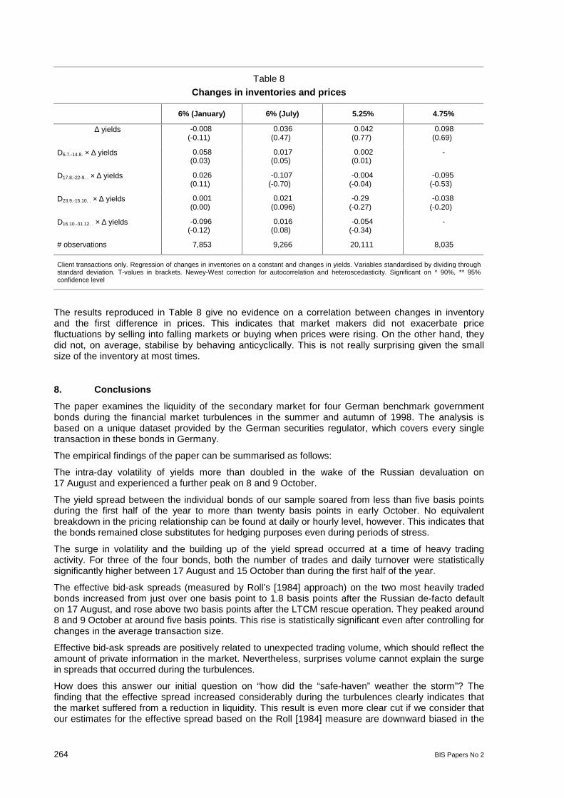
264 BIS Papers No 2
Table 8Changes in inventories and prices
6% (January) 6% (July) 5.25% 4.75%
∆ yields -0.008(-0.11)
0.036(0.47)
0.042(0.77)
0.098(0.69)
D6.7.-14.8. × ∆ yields 0.058(0.03)
0.017(0.05)
0.002(0.01)
-
D17.8.-22-9. . × ∆ yields 0.026(0.11)
-0.107(-0.70)
-0.004(-0.04)
-0.095(-0.53)
D23.9.-15.10. . × ∆ yields 0.001(0.00)
0.021(0.096)
-0.29(-0.27)
-0.038(-0.20)
D16.10.-31.12. . × ∆ yields -0.096(-0.12)
0.016(0.08)
-0.054(-0.34)
-
# observations 7,853 9,266 20,111 8,035
Client transactions only. Regression of changes in inventories on a constant and changes in yields. Variables standardised by dividing throughstandard deviation. T-values in brackets. Newey-West correction for autocorrelation and heteroscedasticity. Significant on * 90%, ** 95%confidence level
The results reproduced in Table 8 give no evidence on a correlation between changes in inventoryand the first difference in prices. This indicates that market makers did not exacerbate pricefluctuations by selling into falling markets or buying when prices were rising. On the other hand, theydid not, on average, stabilise by behaving anticyclically. This is not really surprising given the smallsize of the inventory at most times.
8. Conclusions
The paper examines the liquidity of the secondary market for four German benchmark governmentbonds during the financial market turbulences in the summer and autumn of 1998. The analysis isbased on a unique dataset provided by the German securities regulator, which covers every singletransaction in these bonds in Germany.
The empirical findings of the paper can be summarised as follows:
The intra-day volatility of yields more than doubled in the wake of the Russian devaluation on17 August and experienced a further peak on 8 and 9 October.
The yield spread between the individual bonds of our sample soared from less than five basis pointsduring the first half of the year to more than twenty basis points in early October. No equivalentbreakdown in the pricing relationship can be found at daily or hourly level, however. This indicates thatthe bonds remained close substitutes for hedging purposes even during periods of stress.
The surge in volatility and the building up of the yield spread occurred at a time of heavy tradingactivity. For three of the four bonds, both the number of trades and daily turnover were statisticallysignificantly higher between 17 August and 15 October than during the first half of the year.
The effective bid-ask spreads (measured by Roll’s [1984] approach) on the two most heavily tradedbonds increased from just over one basis point to 1.8 basis points after the Russian de-facto defaulton 17 August, and rose above two basis points after the LTCM rescue operation. They peaked around8 and 9 October at around five basis points. This rise is statistically significant even after controlling forchanges in the average transaction size.
Effective bid-ask spreads are positively related to unexpected trading volume, which should reflect theamount of private information in the market. Nevertheless, surprises volume cannot explain the surgein spreads that occurred during the turbulences.
How does this answer our initial question on “how did the “safe-haven” weather the storm”? Thefinding that the effective spread increased considerably during the turbulences clearly indicates thatthe market suffered from a reduction in liquidity. This result is even more clear cut if we consider thatour estimates for the effective spread based on the Roll [1984] measure are downward biased in the

BIS Papers No 2 265
presence of inventory control and adverse selection effects, which are likely to be importantparticularly in times of great volatility.
Nevertheless, while agents may have faced a higher cost of trading, they were still able to trade. Ourdata does not tell us whether individual agents were able to turn over their position as quickly as theywould have liked, but the fact that the market has been able to sustain a significantly higher thannormal number of trades and volume suggests that such problems were not widespread, if theyoccurred at all. In this sense, liquidity provision has been remarkably effective in dealing with theturbulences, especially when seen in contrast to what happened in the US bond market.
Apart from the issue of financial stability, I mentioned two other reasons for why a central bank shouldmonitor the liquidity in the secondary market for government bonds: the quality of indicators and theborrowing costs of government. Indicator quality clearly suffers if it becomes more costly to trade.Hence our findings provide further evidence for the already widely known fact that indicators are theleast likely to be accurate at times when they are most needed.
The present paper considers only a small, albeit important, segment of the market. It would beinteresting to extend the analysis to a) the futures market, which is far more active than the spotmarket, and b) bonds from other issuers. It would also be of interest to compute a measure of liquiditythat is more robust to the presence of inventory control and adverse selection effects than the Rollmeasure. Both extensions are left for future work.
9. References
Amihud, Y & H Mendelson (1991): “Liquidity, Maturity and the Yields on U.S. Treasury Securities”,Journal of Finance, 66: 1411-25
Andersen, T G, T Bollerslev, F X Diebold & P Labys (1999): “The Distribution of Exchange RateVolatility”, NBER Working Paper 6961
Bagehot, W [pseud.] (1971): “The Only Game in Town”, Financial Analysts Journal, 27: 12-4
Bank for International Settlements (1999a): “International Banking and Financial MarketsDevelopments”, BIS Quarterly Review, March
Bank for International Settlements (1999b): Market Liquidity: Research Findings and Selected PolicyImplications, Report of a Study Group established by the Committee on the Global Financial System ofthe central banks of the Group of Ten countries, May
Bank for International Settlements (1999c): A Review of Financial Market Events in Autumn 1998,Committee on the Global Financial System , October
Bessembinder, H (1994): “Bid-Ask Spreads in the Interbank Foreing Exchange Markets”, Journal ofFinancial Economics, 35: 317-48
Brady, N (1989): Report of the Presidential Task Force on Market Mechanisms, January, Washington,DC: Government Printing Office Choi, J Y, D Salandro & K Shastri (1988) “On the Estimation of Bid-Ask Spreads: Theory and Evidence”, Journal of Financial and Quantitative Analysis, 23(2): 245-69
Davis, E P (1999): “A Reappraisal of Market Liquidity Risk in the Light of the Russia/LTCM GlobalSecurities Market Crisis”, Paper presented to the workshop on “Empirical Research on banksupervision and Structure”, Bank for International Settlements, June 1999
Deutsche Bundesbank (1998): Monthly Report, December
Glosten, L & P Milgrom (1985): “Bid, Ask, and Transaction Prices in a Specialist Market withHeterogeneously Informed Traders”, Journal of Financial Economics, 13: 71-100
Hartmann, P (1999): “Trading Volumes and Transaction Costs in the Foreign Exchange Market:Evidence from Daily Dollar-Yen Spot Data”, Journal of Banking and Finance, 23: 801-24
Hasbrouck, J (1991): “Measuring the Information Content of Stock Trades”, Journal of Finance, 46:178-208
Ho, T & H R Stoll (1981): “Optimal Dealer Pricing under Transactions and Return Uncertainty”, Journalof Financial Economics, 9: 47-73

266 BIS Papers No 2
Ho, T & H Stoll (1983): “The Dynamics of Dealer Markets under Competition”, Journal of Finance, 38:1053-74
Huang, R D & H R Stoll (1997): “The Components of the Bid-Ask Spread: A General Approach”,Review of Financial Studies,10(4):
International Monetary Fund (1998): World Economic Outlook and International Capital MarketsInterim Assessment, December
Kyle, A S (1985): “Continuous Auctions and Insider Trading”, Econometrica, 53(6): 1315-35
Longstaff, F A (1995): “How Much Can Marketability Affect Security Values?”, Journal of Finance,50(5): 1767-74
Madhavan, A (1992): “Trading Mechanisms in Securities Markets”, Journal of Finance, 47: 607-42
O’Hara, M (1995): Market Microstructure Theory, Cambridge MA & Oxford: Blackwell
O’Hara, M & G Oldfield (1986): “The Microeconomics of Market Marking”, Journal of Financial andQuantitative Analysis, 21, December: 361-76
Proudman, J (1995): “The Microstructure of the UK Gilt Market”, Bank of England, Working Paper 38
Roll, R (1984): “A Simple Implicit Measure of the Effective Bid-Ask Spread in an Efficient Market”,Journal of Finance, 39: 1127-40
Stoll, H R (1989): “Inferring the Components of the Bid-Ask Spread: Theory and Empirical Tests”,Journal of Finance, 44(1): 115-34
Vitale, P (1998): “Two Months in the Life of Several Gilt-Edged Market Makers on the London StockExchange”, Journal of International Financial Markets, Institutions and Money, 8: 299-324

BIS Papers No 2 267
FX impact of cross-border M&A
Francis Breedon and Francesca Fornasari, Lehman Brothers
• Globalisation has led to a steady increase in the number of cross-border M&A activities, andso these deals are increasingly discussed in the FX market. However, since M&A activity isstill measured in billions of dollars per month, as compared with the trillion-plus a day tradedin the FX market, it is not clear what impact these deals actually have in practice.
• Using a large sample of past M&A deals, we find that these deals do indeed have an impacton exchange rates, causing, on average, a 1% appreciation of the target nation currencyrelative to the acquirer. We also find that such currency moves can be predicted usingpublicly available data.
• From our results, we construct an M&A currency pressure indicator that can be used to helpinterpret and predict currency moves due to M&A.
Introduction
With globalisation leading to a steady increase in cross-border M&A activity, the latest deals havebecome a common topic of discussion in the FX market. However, cross-border M&A flows are stillonly in the billions of dollars per month, compared with FX turnover estimated at $1.5tr per day and so,despite the interest they generate, it is not clear whether these flows are indeed significant in practice.
Number of cross-border M&A, 1982-1994
1982 1988 1994
UK–US 58 177 180Euro-area1–US 26 67 256
1 France, Italy, Germany. Source: Vasconcellos (1998).
This research note aims to answer three key questions:
1. Does M&A have a significant impact on currencies?
2. Can this impact be predicted using public information available at the time?
3. If there is an impact, how can information on M&A activity best be summarised?
Despite the interest these deals create in the FX market, there are no previous studies to draw on toanalyse this question. Economists seem more interested in the economic motivation for M&A (see forexample Kang [1993] and Vasconcellos [1998]), rather than their impact.
Estimating the impact of M&A
Although the aim is simple, studying the impact of cross-border M&A activity on currencies is oftencomplicated by the intricate financing structure of such deals. We use a event study method (see, forexample, Campbell, Lo and MacKinlay [1997]) with which we test whether the returns to holding thetarget nation’s currency relative to that of the acquirer where cross-border M&A deals have beenannounced is significantly different from zero. By averaging over a large number of similar deals, it canbe determined if there is a consistent excess return.
The first step to estimating excess returns is to construct a sample of deals to analyse. Our sample isbased on information published in the IFR DataBase and includes all transactions that took place in1997-99 and that are greater than US$400m. For simplicity, we concentrate on a subset of possiblecountry pairs: US-euro area, US-UK, US-Canada and US-Japan. The table illustrates some samplestatistics.
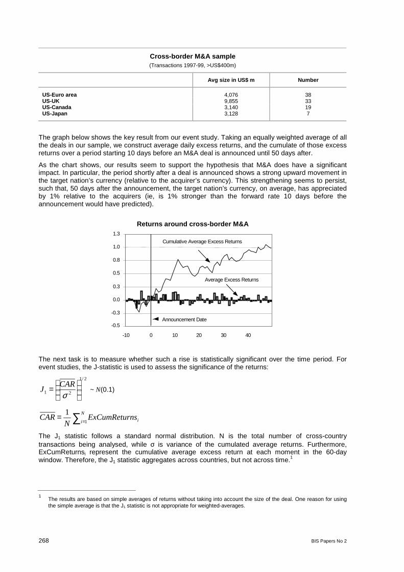
268 BIS Papers No 2
Cross-border M&A sample(Transactions 1997-99, >US$400m)
Avg size in US$ m Number
US-Euro area 4,076 38US-UK 9,855 33US-Canada 3,140 19US-Japan 3,128 7
The graph below shows the key result from our event study. Taking an equally weighted average of allthe deals in our sample, we construct average daily excess returns, and the cumulate of those excessreturns over a period starting 10 days before an M&A deal is announced until 50 days after.
As the chart shows, our results seem to support the hypothesis that M&A does have a significantimpact. In particular, the period shortly after a deal is announced shows a strong upward movement inthe target nation’s currency (relative to the acquirer’s currency). This strengthening seems to persist,such that, 50 days after the announcement, the target nation’s currency, on average, has appreciatedby 1% relative to the acquirers (ie, is 1% stronger than the forward rate 10 days before theannouncement would have predicted).
Returns around cross-border M&A
-0.5
-0.3
0.0
0.3
0.5
0.8
1.0
1.3
-10 0 10 20 30 40
Cumulative Average Excess Returns
Average Excess Returns
Announcement Date
The next task is to measure whether such a rise is statistically significant over the time period. Forevent studies, the J-statistic is used to assess the significance of the returns:
2/1
21
=
σCAR
J ~ N(0.1)
∑ == N
i ieturnsRExCumN
CAR1
1
The J1 statistic follows a standard normal distribution. N is the total number of cross-countrytransactions being analysed, while σ is variance of the cumulated average returns. Furthermore,ExCumReturnsi represent the cumulative average excess return at each moment in the 60-daywindow. Therefore, the J1 statistic aggregates across countries, but not across time.1
1The results are based on simple averages of returns without taking into account the size of the deal. One reason for usingthe simple average is that the J1 statistic is not appropriate for weighted-averages.
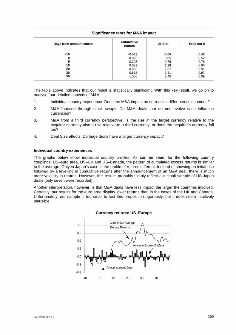
BIS Papers No 2 269
Significance tests for M&A impact
Days from announcement Cumulativereturns J1 Stat Prob not 0
-10 -0.033 -0.06 0.480 0.025 0.05 0.525 0.308 0.76 0.78
10 0.671 1.28 0.9020 0.653 1.37 0.9130 0.862 1.81 0.9750 1.006 2.46 0.99
The table above indicates that our result is statistically significant. With this key result, we go on toanalyse four detailed aspects of M&A:
1. Individual country experience. Does the M&A impact on currencies differ across countries?
2. M&A-financed through stock swaps. Do M&A deals that do not involve cash influencecurrencies?
3. M&A from a third currency perspective. Is the rise in the target currency relative to theacquirer currency also a rise relative to a third currency, or does the acquirer’s currency falltoo?
4. Deal Size effects. Do large deals have a larger currency impact?
Individual country experiences
The graphs below show individual country profiles. As can be seen, for the following countrycouplings, US–euro area, US–UK and US–Canada, the pattern of cumulated excess returns is similarto the average. Only in Japan’s case is the profile of returns different. Instead of showing an initial risefollowed by a levelling in cumulative returns after the announcement of an M&A deal, there is muchmore volatility in returns. However, this results probably simply reflect our small sample of US-Japandeals (only seven were recorded).
Another interpretation, however, is that M&A deals have less impact the larger the countries involved.Certainly, our results for the euro area display lower returns than in the cases of the UK and Canada.Unfortunately, our sample is too small to test this proposition rigorously, but it does seem intuitivelyplausible.
Currency returns: US–Europe
-0.5
-0.3
0.0
0.3
0.5
0.8
1.0
-10 0 10 20 30 40
Cumulative Average
Excess Returns
Average Excess Returns
Announcement Date
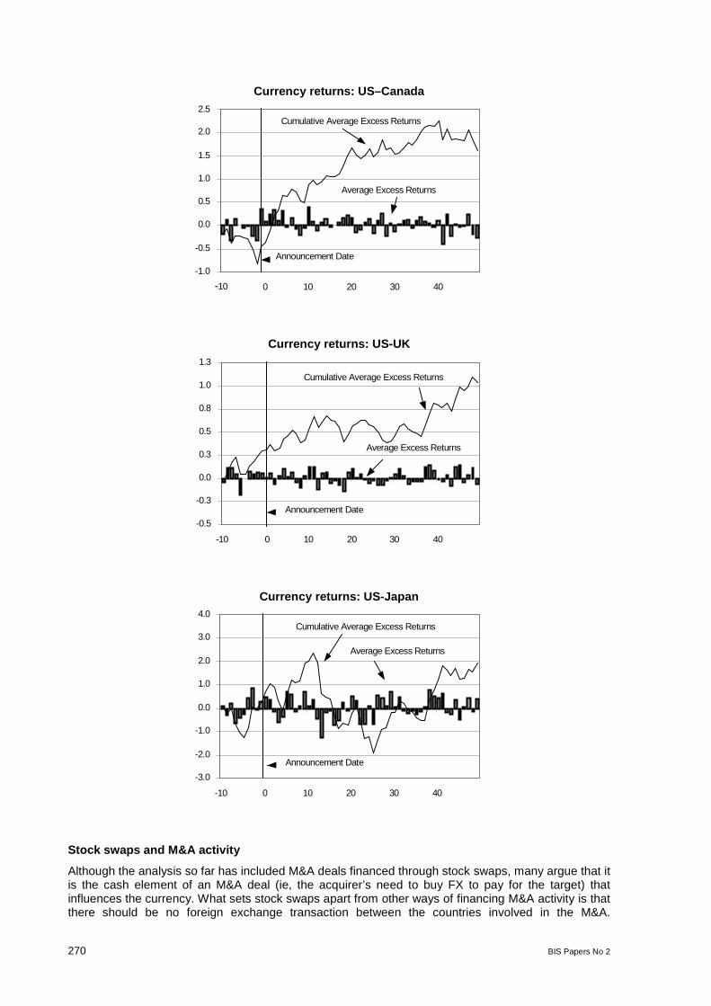
270 BIS Papers No 2
Currency returns: US–Canada
-1.0
-0.5
0.0
0.5
1.0
1.5
2.0
2.5
-10 0 10 20 30 40
Cumulative Average Excess Returns
Average Excess Returns
Announcement Date
Currency returns: US-UK
-0.5
-0.3
0.0
0.3
0.5
0.8
1.0
1.3
-10 0 10 20 30 40
Average Excess Returns
Cumulative Average Excess Returns
Announcement Date
Currency returns: US-Japan
-3.0
-2.0
-1.0
0.0
1.0
2.0
3.0
4.0
-10 0 10 20 30 40
Cumulative Average Excess Returns
Average Excess Returns
Announcement Date
Stock swaps and M&A activity
Although the analysis so far has included M&A deals financed through stock swaps, many argue that itis the cash element of an M&A deal (ie, the acquirer’s need to buy FX to pay for the target) thatinfluences the currency. What sets stock swaps apart from other ways of financing M&A activity is thatthere should be no foreign exchange transaction between the countries involved in the M&A.
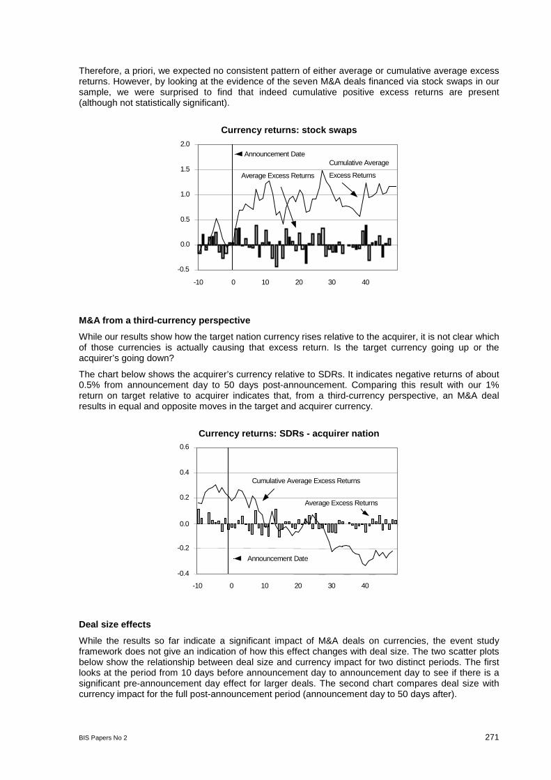
BIS Papers No 2 271
Therefore, a priori, we expected no consistent pattern of either average or cumulative average excessreturns. However, by looking at the evidence of the seven M&A deals financed via stock swaps in oursample, we were surprised to find that indeed cumulative positive excess returns are present(although not statistically significant).
Currency returns: stock swaps
-0.5
0.0
0.5
1.0
1.5
2.0
-10 0 10 20 30 40
Cumulative Average
Excess ReturnsAverage Excess Returns
Announcement Date
M&A from a third-currency perspective
While our results show how the target nation currency rises relative to the acquirer, it is not clear whichof those currencies is actually causing that excess return. Is the target currency going up or theacquirer’s going down?
The chart below shows the acquirer’s currency relative to SDRs. It indicates negative returns of about0.5% from announcement day to 50 days post-announcement. Comparing this result with our 1%return on target relative to acquirer indicates that, from a third-currency perspective, an M&A dealresults in equal and opposite moves in the target and acquirer currency.
Currency returns: SDRs - acquirer nation
-0.4
-0.2
0.0
0.2
0.4
0.6
-10 0 10 20 30 40
Cumulative Average Excess Returns
Average Excess Returns
Announcement Date
Deal size effects
While the results so far indicate a significant impact of M&A deals on currencies, the event studyframework does not give an indication of how this effect changes with deal size. The two scatter plotsbelow show the relationship between deal size and currency impact for two distinct periods. The firstlooks at the period from 10 days before announcement day to announcement day to see if there is asignificant pre-announcement day effect for larger deals. The second chart compares deal size withcurrency impact for the full post-announcement period (announcement day to 50 days after).
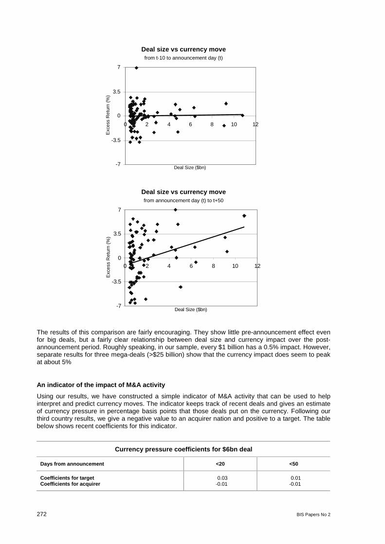
272 BIS Papers No 2
Deal size vs currency movefrom t-10 to announcement day (t)
-7
-3.5
0
3.5
7
0 2 4 6 8 10 12
Deal Size ($bn)
Exc
ess
Ret
urn
(%)
Deal size vs currency movefrom announcement day (t) to t+50
-7
-3.5
0
3.5
7
0 2 4 6 8 10 12
Exc
ess
Ret
urn
(%)
Deal Size ($bn)
The results of this comparison are fairly encouraging. They show little pre-announcement effect evenfor big deals, but a fairly clear relationship between deal size and currency impact over the post-announcement period. Roughly speaking, in our sample, every $1 billion has a 0.5% impact. However,separate results for three mega-deals (>$25 billion) show that the currency impact does seem to peakat about 5%
An indicator of the impact of M&A activity
Using our results, we have constructed a simple indicator of M&A activity that can be used to helpinterpret and predict currency moves. The indicator keeps track of recent deals and gives an estimateof currency pressure in percentage basis points that those deals put on the currency. Following ourthird country results, we give a negative value to an acquirer nation and positive to a target. The tablebelow shows recent coefficients for this indicator.
Currency pressure coefficients for $6bn deal
Days from announcement <20 <50
Coefficients for target 0.03 0.01Coefficients for acquirer -0.01 -0.01

BIS Papers No 2 273
These coefficients represent the expected daily return of being long of the target nation currency whena deal averaging US$5.8bn is announced. Following the results on deal size, when constructing thisindicator we give a larger weight to larger deals (though with a cutoff for “mega-deals”).
Given that our results for individual countries implied – but did not prove – that an M&A deal of a givensize has a smaller impact the larger the countries involved, we also present a GDP-weighted versionof our indicator.
M&A currency pressure indicator – 6 July 1999(% bp per day)
Country Unweighted GDP-weighted
Australia 0.34 4.94Canada 0.48 4.55Chile 0.16 12.22Czech Republic 0.10 10.47Denmark -0.17 -5.60Euro -1.25 -1.08Greece -0.75 -33.02Norway 0.41 14.60Poland 0.07 2.72Singapore 0.08 4.20South Korea 0.14 1.66Sweden 0.18 4.22Switzerland -0.52 -9.34United Kingdom 1.15 5.25United States -0.41 -0.30
Conclusion
As well as confirming the widely held market belief that cross-border M&A activity does influenceexchange rates, our analysis shows:
1. The appreciation tends to occur after the public announcement of the deal and so does notrely on inside information.
2. Statistical tests confirm that this excess return is statistically significant (at the 99% level)and so is probably not just a quirk of our data.
3. Separate tests on deals that do not involve cash (ie, stock swaps) indicate that these toohave a currency impact.
4. From a third-currency perspective, currency moves around M&A tend to lead to a fall in theacquirer currency and a rise in the target currency of equal size.
Using our results, we are now in a position to monitor M&A effects on currencies which are clearly animportant supplement to standard economic analysis.
References
J Campbell, A. Lo, A. MacKinlay, 1997: The Econometrics of Financial Markets, Princeton UniversityPress, USA.
J K Kang, 1993: “The international market for corporate control. Mergers and acquisitions of US firmsby Japanese firms” Journal of Financial Economics, 34, p345-371.
G M Vasconcellos, R J Kish, 1998: “Cross-border mergers and acquisitions: the European–USexperience,” Journal of Multinational Financial Management, 8, p431-450.