market intraday momentu m and retu rn predictability
TRANSCRIPT

See discussions, stats, and author profiles for this publication at: https://www.researchgate.net/publication/339877949
Intraday momentum and return predictability: Evidence from the crude oil
market
Article in Economic Modelling · March 2020
DOI: 10.1016/j.econmod.2020.03.004
CITATION
1READS
409
4 authors, including:
Some of the authors of this publication are also working on these related projects:
Knights and dames on the board of directors View project
Commodity options View project
Zhuzhu Wen
Huazhong University of Science and Technology
6 PUBLICATIONS 222 CITATIONS
SEE PROFILE
Diandian Ma
University of Auckland
16 PUBLICATIONS 50 CITATIONS
SEE PROFILE
Yahua Xu
Central University of Finance and Economics
12 PUBLICATIONS 4 CITATIONS
SEE PROFILE
All content following this page was uploaded by Yahua Xu on 19 March 2020.
The user has requested enhancement of the downloaded file.

1
Intraday momentum and return predictability: Evidence from the
crude oil market
Zhuzhu Wena, Xu Gongb, Diandian Mac, Yahua Xu*,d
a School of Management, Huazhong University of Science and Technology
b School of Management, China Institute for Studies in Energy Policy, Collaborative Innovation Center for Energy
Economics and Energy Policy, Xiamen University
c Graduate School of Management, University of Auckland
d China Economics and Management Academy, Central University of Finance and Economics
Abstract
Intraday return predictability has firstly been identified in the equity markets, and we extend the
analysis to the crude oil market by using high-frequency United States Oil Fund data from 2006 to
2018. We find a different intraday prediction pattern in the oil market, where only the first half-hour
returns positively predict the last half-hour returns. A market timing strategy based on the findings
generates substantial profits. We further decompose the first half-hour return into the overnight and
the open half-hour components, and find that the former contains more predictive information.
Economic mechanisms of the infrequent portfolio rebalancing and the presence of late-informed
investors explain our findings. Notably, unlike equity markets, the oil market exhibits a unique intraday
trading volume pattern, caused by the release of two routine oil inventory announcements. However,
the information contained in the inventory announcements does not offer predictability to the last half-
hour returns.
JEL classification: G1; C5; Q3; Q4
Keywords: Intraday momentum, return predictability, crude oil market, market timing strategy

2
Acknowledgments: We are especially grateful to Sushanta Mallick (editor) for guidance and to two anonymous referees
for insightful comments that have significantly improved the paper. We appreciate the comments and suggestions provided
by participants at the 2019 International Conference on Energy Finance, China.
* Corresponding author: China Economics and Management Academy, Central University of Finance and Economics, No.
39 South College Road, Haidian District, 100081 Beijing, China. Email [email protected].

3
1. Introduction
Momentum is one of the most famous and well-documented market anomalies which seems to
contradict with the efficient market hypothesis. Traditional cross-sectional momentum has firstly been
proposed by Jegadeesh and Titman (1993) and continued to gain the interest of researchers and
practitioners: buying stocks that perform well and selling stocks which perform badly over the past
several months, produces substantial profits over the next 3 to 12 months and outperforms other
benchmark investment strategies (e.g., Griffin et al., 2003; Grinblatt et al., 1995; Jegadeesh and Titman,
2001). Besides, the later work of Moskowitz et al. (2012) documents time-series momentum: the past
12-month excess return of each asset can positively predict its future return in the next one month. The
prevalence of time series momentum can extend to a wide range of assets, including currencies,
commodities, and bonds, an asset’s past performance can predict its future returns (e.g., Asness et al.,
2013; Miffre and Rallis, 2007; Moskowitz et al., 2012; Orlov, 2016). Research on momentum has
important implications for portfolio investors, risk managers, and policy makers for better
understanding the mechanism of an efficient financial market. However, despite decades of empirical
research on momentum, most studies have been confined to momentum patterns occurring on a weekly
or monthly basis, using low-frequency daily or monthly data.
Along with the rapid development of High-Frequency Trading (HFT), intraday trading has
gained increasing popularity among practitioners, as the trading algorithms catch more trading
opportunities by detecting small price fluctuations from multiple markets. 1 The HFT also
consequently enhances liquidity in the market. While with the availability of a large amount of intraday
trading data, little focus has been put on the issue of intraday momentum, namely, intraday
predictability patterns across a trading day, until recently. Intraday momentum was first documented
by Gao et al. (2018), who find that, in the U.S. equity index market, during any trading day, the first
and the second-to-last half-hour returns can significantly predict the last half-hour returns. Zhang et al.
(2019a) report similar findings in relation to the Chinese equity index market. Beyond equity markets,
Elaut et al. (2018) and Jin et al. (2019) document intraday momentum in foreign exchange markets
1 For example, the high-frequency trading volume in New York Stock Exchange (NYSE) between 2005 and 2009 has
grown by about 164% (Charles, 2009).

4
and in Chinese commodity futures markets, respectively. Although momentum patterns at the intraday
level is an ongoing topic that attracts increasing interest from academics and practitioners, HFT
receives harsh critiques due to big market fluctuations and uncertainties caused by large-scale order
placements or cancellations made in milliseconds.2 Therefore, research on the intraday predictability
and high-frequent trading helps regulators understand the HFT market mechanism and assist them in
making decisions on regulating the markets that take into account investor behaviours and their instant
effects on markets.
We are motivated to investigate whether and to what extent intraday predictability patterns exist
in the crude oil market for two major reasons. First, numerous studies find strong connections between
crude oil and stock markets (e.g., Fenech and Vosgha, 2019; Hou et al., 2019; Wang et al., 2019).
Nandha and Faff (2008) show that oil price rise by affecting economic activity and subsequently leads
to negative stock market reactions. Pönkä (2016) finds that oil prices outperform other common
predictors in regarding the direction of stock returns in the U.S. and other markets. However, research
on such connections is restricted to medium and long horizons, and the literature does not cover
whether momentum patterns exist in a trading day in the oil market. Moreover, explanations of intraday
momentum in the equity markets are from the angle of trading behaviors, investor sentiment, and the
degree of information content at different trading intervals (Gao et al., 2018; Renault, 2017; Zhang et
al., 2019a), and no study has examined whether and why intraday momentum exists in the oil market.
Therefore, considering the close link between oil market and the economy, further exploration for
intraday trading mechanism of oil market provides more crystal insights for policy makers to maintain
its stability and reduce impacts of oil shocks on the economy.
We empirically test our hypothesis by employing the high-frequency United States Oil (USO)
Fund data for several reasons. Firstly, the crude oil market is one of the most important energy
commodity markets, its related futures, options and exchange-traded funds (ETFs) are gaining
increasing popularity and are actively traded. The ETFs, in particular, are becoming one of the most
important investment vehicles due to low transactions costs, tax efficiency, and equity-like features
2 One example is that on 6 May, 2010, the Dow Jones Industrial Average (DJIA) declined 10% in 20 minutes before
rising again, which is the largest intraday drop recorded (Investopedia, 2019a).

5
(e.g., Lettau and Madhavan, 2018). Second, since USO is specifically designed for short-term investors
who closely monitor their positions and pay attention to volatility, it fits our intraday momentum
research design (Investopedia, 2019b). Third, the pioneering study of intraday momentum by Gao et
al. (2018) implement the study of stock market intraday momentum by using S&P 500 ETF data. Note
that the trading hours for ETF products are normally from 9:30 a.m. to 4:00 p.m. Eastern Standard
Time (EST), while the trading hours for WTI futures are different from the equity market. Therefore,
regarding consistent trading periods, USO is a good proxy for an analysis similar to that of Gao et al.
(2018) in the crude oil market.
We thus conduct a pioneering study to test for intraday momentum in the oil market.
Understanding the predictability pattern of the oil market can provide insights for future research about
the connections between the equity and oil markets at the intraday level. Second, it is commonly known
that the addition of commodities, such as oil and silver, to a portfolio can reduce overall portfolio risk.
Nandha and Faff (2008) state that an internationally diversified portfolio can be further diversified by
including assets with positive correlations to oil price changes. Exploration of price movements in the
oil market not only facilitates a deeper academic understanding of the crude oil market’s microstructure,
particularly its intraday momentum patterns and return characteristics, but also provides practical
implications for high-frequency traders and investors who consider adding oil products to their
portfolios. It also provides more thorough insights for policy marker to better understanding the HFT
mechanism of oil market.
We have several remarkable findings. Firstly, our study reveals that the first half-hour return of a
trading day significantly predicts the last half-hour return of that day, both in sample (IS) and out of
sample (OS). For the IS analysis, the predictive value is 0.729%, and our OS analysis further confirms
the predictive power of the first half-hour returns, with an OS R-square, with value of 0.659%, where
both are economically sizable and much higher than monthly predictors (Rapach and Zhou, 2013).
Moreover, we further decompose the first half-hour return into overnight component and open half-
hour component, and find that the former is the main contributor for prediction. One notable difference
between crude oil and equity market is that studies (e.g., Gao et al., 2018; Zhang et al., 2019a) show
that the second-to-last half-hour returns also have predictive power in equity markets, we find no such
6
intraday predictability pattern in the crude oil market. Such distinction highlights the essential
difference between crude oil and equity markets. Subsequently, investors in the two markets should
take different investing strategies to utilize the different intraday predictability patterns.
The empirical findings can be theoretically explained by infrequent portfolio rebalancing (e.g.,
Bogousslavsky, 2016) and the presence of late-informed investors (e.g., Baker and Wurgler, 2006;
Cohen and Frazzini, 2008; Huang et al., 2015). We also compare the intraday trading volume pattern
in the crude oil market with that in the equity markets, documented by Gao et al. (2018) and Zhang et
al. (2019a). We find that, although a perfect U-shaped trading volume pattern is observed in the equity
markets, it does not arise in the crude oil market, and such difference causes the distinct intraday
predictability pattern of the two markets. In particular, we note two additional trading volume spikes
in the 3rd and 10th half hours, corresponding to the release of two routine intraday announcements in
the crude oil market: the Weekly Petroleum Status Report, released at 10:30 a.m. by the U.S. Energy
Information Administration, and the weekly survey report about the energy market, released around
2:00 p.m. by Reuters. Except for the spikes in the 3rd and 10th half-hour intervals, the trading volume
generally diminishes from the second half hour, until a substantial increase in the last half hour.
Secondly, as the intraday predictability varies across crisis and non-crisis periods, we split our
sample into crisis and non-crisis periods, with the former encompassing two crises: the global financial
crisis of June 1, 2008, to January 31, 2009, and the oil market crisis of June 1, 2014, to January 31,
2016 (e.g., Gao et al., 2018). We find that predictability is especially strong during the crisis periods,
with a predictive value of 1.923%: this level of predictability substantially exceeds the predictive
value of 0.335% during the non-crisis periods. As explained by Elaut et al. (2018), the stronger intraday
momentum in foreign exchange market during crisis is mainly caused by risk aversion for overnight
inventory and high liquidity demand during market opening.
Thirdly, we also find that the predictive power of the first half-hour returns is stronger when the
first half hour’s trading has higher realized volatility, higher trading volume, and significant overnight
return jumps, all of which are associated with high overnight uncertainty. Moreover, our further
analysis shows that the intraday momentum is stronger on positive jump days than on negative ones,

7
with positive (negative) jumps usually characterized by the overnight release of good (bad) news,
which suggests it is more sensitive to good market news.
Fourthly, our next step is to assess the economic values by using the predictability of the first
half-hour return, as a trading signal in the market timing strategy. Specifically, if is positive
(negative), we take a long position at the beginning of the first half hour and close the position at the
end of the last half hour. Our results show that this market timing strategy significantly outperforms
two other benchmark strategies, namely, the always-long and the buy-and-hold strategies, since it
generates a higher average return, along with a lower standard deviation and a higher Sharpe ratio.
Therefore, by utilizing the intraday predictability in crude oil market, practitioners can gain substantial
profits which is of great practical importance.
Our study makes an important contribution to the existing literature of intraday momentum by
extending the analysis to crude oil market (e.g., Heston, 2010; Murphy and Thirumalai, 2017). To the
best of our knowledge, it is also the first effort to examine, using the USO ETF data, intraday
momentum in the crude oil market. It provides important practical implications for market traders and
policy makers for deeper understanding of the HFT trading mechanism in crude oil market. The
different intraday momentum patterns between the crude oil and equity markets suggest the essential
distinction between the two markets, which can be related to the different patterns of intraday trading
volumes. Since USO is one of the largest and most liquid crude oil ETFs in the world and crude oil is
one of the most important commodity markets, the results can serve as a useful reference for other
commodity markets.
Moreover, our analysis focuses on the U.S. ETF market, which can provide important economic
implications for broader cases. For example, among the limited existing literature, Jin et al. (2019)
investigate intraday momentum in Chinese commodity futures contracts: copper, steel, soybean and
soybean meal, and find that the open market component (i.e., return for the first half-hour after market
open) is the dominant role in intraday prediction. In sharp contrast, our research in the U.S. oil ETF
market, the overnight component (i.e., return from previous market close to next day’s market open)
contribute most predictability. One possible explanation is that in oil market intraday momentum is
more closely related to day trading liquidity provision (e.g., Elaut et al., 2018), while in Chinese

8
agricultural and metal commodity markets it is more likely to be affected by the behaviour of informed
traders (e.g., Bogousslavsky, 2016). The different sources of prediction highlight the distinct
mechanisms among various markets and the future direction for full-round research.
The structure of the remainder of our paper is as follows. Section 2 is the main empirical analysis
part, which contains description of our data and methodology and corresponding empirical findings.
Section 3 examines the economic implications of the first half-hour returns, and offers economic
explanations for the intraday momentum and a unique trading volume pattern observed in the crude
oil market. Section 4 concludes the paper.
2. Empirical analysis
2.1 Data and methodology
We use the one-minute intraday prices of the USO ETF to calculate half-hour returns for the crude oil
market. Our transaction data, obtained from Thomson Reuters DataScope Select, include the close bid,
close ask, the number of trades, and the trading volume from April 10, 2006 to December 4, 2018.
Following Gao et al. (2018), we exclude trading days with fewer than 500 trades. Our final sample
includes 3,171 trading days.
For each day 𝑡 we compute the first half-hour return 1,tr by subtracting the previous trading
day’s close price from the price at 10:00 a.m., where 1,tr contains information released after the
previous day’s trading.3 We compute all half-hour returns from 9:30 a.m. to 4:00 p.m. by using the
following equation, which leads to 13 half-hour returns per trading day:
( ) ( ), , 1, , 1,2, ,1log lo 3,gi t i t i tp ir p − = = − (1)
where ,i tp denotes the price on the ith half hour on day t. Note that 0,tp is the close price of the
previous trading day at 4:00 p.m.
Table 1 shows the descriptive statistics of all the half-hour returns across the day. Compared with
the other half-hour returns of the day (i.e., 𝑟2, 𝑟3, … , 𝑟12), the first half-hour returns (𝑟1) have the lowest
3 To control for non-normality, we use the natural logarithm of USO ETF prices to calculate returns.

9
minimum, the highest maximum, the largest standard deviation, and the lowest kurtosis. In contrast,
the last half-hour returns (𝑟13) have the highest minimum the lowest maximum the highest positive
skewness, and a low standard deviation compared to the other half-hour returns. The larger distribution
of the first half-hour returns reveals that they might contain more important market information
compared to their last half-hour counterparts.
[Insert Table 1 about here]
2.2 Predictive analysis
We first test the intraday momentum by checking whether the market’s first half-hour return predicts
the last half-hour return on the same day, using the following Regression:
13, 1,t t tr r = + + , t = 1, 2,…,T, (2)
where 1,tr and 13,tr denote the first and last half-hour returns on day t, respectively, and T is the total
number of trading days. We focus on the first and last half hours because they are the most active
trading times on a typical trading day. Price-sensitive news released before the market opens increases
the likelihood of large price moves during the first half hour of trading. Such news is also likely to
create a larger gap between the opening price and the closing price, thereby creating a significant
overnight return. Trading activity diminishes after the first half hour (Gao et al., 2018).
To realize portfolio returns and avoid after-hours risks, institutional traders and professionals
actively exit their positions in the last half hour, an action that again prompts a large volume and high
volatility in the market. As reported by The Wall Street Journal, “more than 25 percent of all trading
at the NYSE happens after 3:30 p.m. EST, the final half-hour trading” (wsj.com).4 Our results in Panel
A of Table 2 show that the first half-hour return (i.e., 1r ) has positive predictive power for the last
half-hour return (i.e., 13r ) at the 1% significance level, with an 2R value of 0.729%, indicating strong
intraday momentum in the crude oil market. Notably, the in-sample 𝑅2 value is much lower than its
counterpart in U.S. (Gao et al., 2018) and Chinese equity markets (Zhang et al., 2019a), but still it is
4 “What’s the biggest trade on the New York Stock Exchange? The last one,” March 2018, retrieved February 6, 2019,
from wsj.com.

10
much higher than monthly predictors (e.g., Rapach and Zhou, 2013). The positive slope indicates that
if the first half-hour return (i.e., 1r ), constructed from the previous trading day’s market close, is
positive (negative), then the last half-hour return also tends to be positive (negative), suggesting that
good (bad) market news released the previous night still has a positive (negative) impact on today’s
last half trading hour.
[Insert Table 2 about here]
Prior research, most notably work by Gao et al. (2018), also documents the significant
predictability of the second-to-last half-hour return (i.e., 12r ) for the last half-hour return (i.e., 13r ) in
U.S. equity market, mainly because intraday prices persist across the trading day. Moreover, the
predictive information carried by the first and second-to-last half-hour returns are distinctive and
independent, with the former carrying larger predictive power, demonstrated by higher in-sample 2R .
Later work of Zhang et al. (2019a) also identifies the independent and complementary predictability
of the first and second-to-last half-hour returns in Chinese equity market, whereas the second-to-last
half-hour return exhibits higher in-sample 2R . We use the same approach as Gao et al. (2018) to assess
the predictive power of 12r in the crude oil market; specifically, we use the USO ETF sample and
regress the last half-hour return on the 12th half-hour return:
13, 12, , 1,2, , .t t t t Tr r = + + = (3)
The second column of Panel A in Table 2 shows that the coefficient of 12r is not statistically
significant, suggesting that the second-to-last half-hour return does not predict the last half-hour return
in the crude oil market. This finding is inconsistent with that of prior studies based on equity markets
because the intraday price persistence is low in the crude oil market. Therefore, the trading strategies
of high-frequency traders in the crude oil market should differ from those used in equity markets, only
the first half-hour returns in oil market exhibit predictive power. More economic explanations about

11
such difference will be detailed in the later part. Because we find that 12r is not an efficient predictor
in the crude oil market, we consider only the predictor 1r in our analyses hereafter.5
2.3 OS analysis
Although our IS analysis in the previous section reveals the existence of intraday momentum in the
crude oil market, we recognize that IS predictability could be attributed to overfitting issues and might
not, therefore, imply OS predictability (Welch and Goyal, 2008). However, OS predictability is very
valuable to practitioners, because it can help them predict returns and make trading decisions. With
this point in mind, we perform an OS analysis by running monthly frequency regressions based on a
recursive estimation window to assess the robustness of intraday momentum in the crude oil market
(e.g., Henkel et al., 2011; Lettau and Nieuwerburgh, 2008; Rapach et al., 2010; Zhang et al., 2019b;
Zhang et al., 2019c).
We begin our analysis by splitting our sample observations into an IS subset that contains m
observations, from April 10, 2006 to December 31, 2009, similar to previous work of Gao et al. (2018)
and Zhang et al. (2019a); and an OS subset that contains the remainder of the q observations, from
January 1, 2010 to December 4, 2018. We then take the parameters m and m, generated by applying
regression (2) to the m IS observations and use the following equation to calculate the first predicted
OS 13, 1mr + :
13, 1 1, 1, 1m m m mr r + += + . (4)
where 1r ,m+1 is the actual first half-hour return of m + 1 observations. We then calculate the next OS
forecast, 13, 2mr + , as
13, 2 1 1, 1 1, 2m m m mr r + + + += + , (5)
where 1m + and 1, 1m + are the parameters generated by applying regression (2) to the m + 1
observations, and 1r ,m+2 is the actual first half-hour return of m + 2 observations. Continuing in this
5 We conduct a predictive analysis of the other half-hour returns but find no significant predictive power.

12
manner, we obtain q OS forecasts 13r . We then use the OS 2
OSR statistic to evaluate the performance
of the predictive model, defined as follows:
( )
( )
2
13, 13,2 12
13, 13,1
ˆ1
T
t ttOS T
t tt
r rR
r r
=
=
−= −
−
, (6)
where 13,ˆ
tr denotes the last half-hour return predicted by the sample up to 𝑡 − 1, and 13,tr is the
historical average return for the corresponding period. If 2
OSR is positive, the OS predictability
surpasses the predictability of the historical average (Campbell and Thompson, 2008).
Panel B of Table 2 presents the OS results. As evident, the OS R-square value, 2
OSR , has a positive
value of 0.659%, with a 1% significance level, indicating that the OS forecast offers better
predictability than the historical average. This result, in turn, confirms the persistence of intraday
momentum in the OS analysis. Unlike to the equity markets where the second-to-last half-hour return
also exhibits predicability, only the first half-hour returns exhibit significant predictability in crude oil
market, for both in- and out-of-sample analysis, highlighting the essential differences between crude
oil and equity markets.
2.4 Subperiod analysis: Oil crisis periods
Various studies document that the standard monthly momentum strategy performs weakly during
financial crises in equity markets (e.g., Li and Tsiakas, 2017; Lin et al., 2017; Rapach et al., 2010;
Wang et al., 2018). Moreover, recent research about intraday momentum in the equity markets also
confirms that the patterns differ for the crisis and non-crisis periods. More specifically, Gao et al. (2018)
find that the predictability of first and second-to-last half-hour returns are much stronger during the
Global Financial Crisis (GFC) period in the U.S. equity market, whereas Zhang et al. (2019a) identify
the opposite pattern in the Chinese equity market, that is, the intraday momentum is much stronger
during the non-GFC period. Along this line, we are interested in investigating if the intraday
momentum persists in the oil market during crises. We consider two specific oil market crisis periods,
identified by Singh et al. (2018): from June 1, 2014, to January 31, 2016, and June 1, 2008, to January

13
31, 2009, rather than GFC in this section. For comparative purposes, we conduct the predictability
analysis for the oil-crisis and non-oil-crisis periods.
[Insert Table 3 about here]
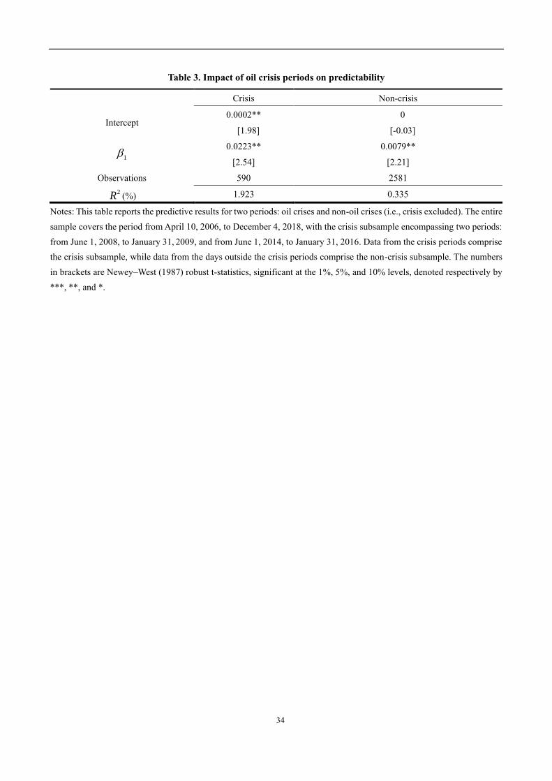
Table 3 reports the results. The slope 1 has a significance level of 5% for both the crisis periods
(i.e., June 1, 2008, to January 31, 2009, and June 1, 2014, to January 31, 2016) and the non-crisis
periods, indicating that the predictability of 1r remains strong throughout the entire sample period,
despite market fluctuations during the two oil market crises. Note, in particular, in Table 3, that
although the sample size of the crisis period is less than 25% of that of the non-crisis periods, the
magnitude of 1 for the crisis period (0.0223) is nearly three times of its counterpart for the non-
crisis periods (0.0079). Also that the 2R value for the crisis periods (1.923%) substantially exceeds
that for the non-crisis periods (0.335%). In all, these results jointly suggest that the predictability of
1r remains significant for both the crisis and non-crisis periods, but is much stronger during crises. It
suggests that the intraday momentum is stronger during oil crisis periods. Stronger intraday momentum
in RUB–USD currency market during crisis periods is also found by Elaut et al. (2018), which can be
attributed to the risk aversion to overnight holdings and increasing liquidity demand by market
participants during the next day’s market open, that is, the first half-hour of trading. Facing rising level
of overnight uncertainty during crisis, investors are more inclined to offload inventories before the
market close due to risk aversion to overnight holdings (e.g., Bjønnes and Rime, 2005). Since crisis
periods are characterized by high market volatility, in the later part of this work, we further analyze
intraday momentum in the crude oil market under various volatility regimes.
The next step in our investigation is to look at the time trends of the predictability by 1r , that is,
the slope of 1r . Figure 1 presents the time-varying slopes of 1r estimated recursively over time. After
minor initial volatility, the slope of 1r stays relatively stable until it is disturbed by the crude oil crisis,
starting in mid-2014. Then, after a continuous decrease throughout the crisis period, it sharply climbs
and rises above its pre-crude oil crisis level and remains stable after that. Figure 1 suggests that, overall,
the slope of 1r is stable, which indicates that the intraday momentum pattern is stable. Equally

14
interesting is the fact that, when the slopes of 1r are destabilized by the fluctuating crude oil crisis,
the predictability of 1r becomes much stronger for the post-crisis period.
[Insert Figure 1 about here]
2.5 Trading patterns across the day
In the previous analysis, we find that the predictability of first half-hour returns differ under various
market situations. To further explore the regime behind such difference, we investigate the intraday
trading behavior of oil prices in this section. More specifically, we present a series of graphs that
summarize oil market trading patterns, measured in terms of realized volatility and trading volume of
the USO ETF from April 10, 2006, to December 4. 2018. Since trading hours are from 9:30 a.m. to 4
p.m., each trading day includes 13 30-minute subintervals, labeled from one to thirteen in Figures 2 to
3.
Figure 2 plots the 30-minute average realized volatility, which is calculated using Equation (A.1)
in the Appendix. Note that the highest realized volatility in Figure 2 occurs in the first half hour, driven
by the overnight information, as discussed previously. From the first half hour to the second half hour
of trading, realized volatility drops by more than 60% and then continues the decreasing trend, except
for a remarkable spike in the third half hour corresponding to a routine inventory announcement at
10:30 a.m., usually every Wednesday. This shows that the market’s response to the overnight
information was strongest in the first half hour and quickly stabilized after the third half hour, and the
oil market also reacts to routine inventory announcements. Intuitively, the two largest intraday spikes,
occurred in the first and third half hour, may contain more important market information compared to
the others. Detailed statistical analysis will be implemented in the latter part.
[Insert Figure 2 about here]
Figure 3 plots the 30-minute average trading volume, which exhibits a perfect U-shape in the
equity market (e.g., Gao et al., 2018). Just as the pattern for realized volatility, the trading volume
peaks during the first half hour of the trading day. However, unlike the pattern in Figure 2, there is no

15
sharp decrease in trading volume in the second half hour. Except for spikes in the 3rd and 10th half
hours, trading activity generally cools down from the second half hour. The two additional spikes in
the 3rd and 10th half hours, which do not exist in equity markets, intrigue and motivate us to analyze
their driving force in Section 4. Of greater importance, however, is the substantial jump in trading
volume during the last half hour, a pattern that captures the fact that institutional traders and
professionals actively exit positions to realize portfolio returns and avoid after-hours risks. Therefore,
the relatively active intraday trading in the first, third, tenth and last half hours attracts our attention.
[Insert Figure 3 about here]
2.6 Volatility, trading volume, overnight return, and jumps
Our previous results reveal that the intraday momentum shows stronger predictability during crises,
those periods characterized by higher volatility. This pattern thus raises the question of what role
volatility plays in intraday momentum in the crude oil market. For high-frequency traders, volatility is
the primary ingredient for making a profit; understanding volatility therefore offers opportunities to
capitalize on intraday momentum. We endeavor to answer this question by referring to Gao et al. (2018)
and ordering our sample of 3,171 trading days according to volatility realized in the first half hour. We
split the ordered sample into three subgroups, of low, medium, and high volatility. Each subsample
consists of 1,057 trading days.
Panel A of Table 4 presents the extent to which the crude oil market’s first half-hour return, 1r ,
predicts the last half-hour return, 13r . We generate 1r and 13r by applying regression (2) to each
subsample of different volatility levels. The results, summarized in the panel, show that the only 1
that is statistically significant at the 1% level is the one generated by the high-volatility subsample, a
finding that indicates that, in a highly volatile crude oil market, the first half-hour returns strongly
predict the last half-hour returns. Note also that the significance of 1 and 2R increases markedly
with volatility, suggesting that stronger intraday momentum corresponds to higher volatility. The
finding is consistent with previous research in equity markets (e.g., Gao et al., 2018; Zhang et al.,

16
2019a), as suggested by Zhang (2006) the greater the market uncertainty, the stronger the price
persistence.
[Insert Table 4 about here]
In keeping with recent studies exploring momentum in equity markets (e.g., Gao et al., 2018;
Zhang et al., 2019a), we also analyze the impact of trading volume on the first half-hour returns in the
crude oil market. After sorting all sample trading days by their first half-hour trading volumes, we split
the whole sample into three equal-sized subgroups, of low, medium, and high volume. We then
calculate the OS 2R value for each group. Panel B of Table 4 presents the results. These results show
that the estimated coefficient 1 is statistically significant at the 5% level for both the medium- and
high-volume subsamples. Additionally, like the results in Panel A, the values of 1 and OS 2R
increase substantially as trading volume increases, indicating increasing predictability of first half-
hour returns. These results suggest that the correlation between intraday momentum and trading
volume is highly positive in crude oil market, similar to that of the equity market (e.g., Gao et al.,
2018).6
As discussed previously, price-sensitive news released after trading hours increases the likelihood
of pre-market moves and overnight returns. We therefore explore how the intraday momentum
performs on days that differ in terms of overnight return levels. We calculate the overnight returns by
using Equation (1), where i = 1, and then order the entire sample of trading days according to the
absolute values of overnight returns. This step allows us to divide the sample into three subsamples of
equal size but differentiated according to low, medium, and high overnight returns.
Panel C of Table 4 presents the predictive power of the crude oil market’s first half-hour return,
1r , generated by applying each subsample to regression (2). The high-level overnight return subsample
produces a highly significant 1 and an impressive 2R value of 1.508%, whereas the other two
6 We also order our sample according to the total trading volume on each trading day and find no significant differences
between the results of the analysis based on the total trading volume and the analysis based on the first half-hour’s trading
volume.

17
subsamples produce an insignificant 1 along with much lower 2R values. These results indicate
that the predictability of first half-hour returns are closely related with overnight returns. To further
verify this hypothesis, we decompose the first half-hour return (i.e., 1,tr ) into two components:
overnight return from the previous market close to market open at 9:30 a.m. (i.e., 16:00 9:30,tr −
) and open
half-hour return from the market open to the end of first half-hour at10:00 a.m. (i.e.,9:30 10:00,tr −
). We
then investigate the predictability of the two components by running the following econometric
specifications:
9:30 10:0013, 9:30 10:00, , 1, 2, , ,t r t tr r t T − −= + + = (7)
16:00 9:3013, 16:00 9:30, , 1, 2, , ,t r t tr r t T − −= + + = (8)
9:30 10:00 16:00 9:3013, 9:30 10:00, 16:00 9:30, , 1, 2, , .t r t r t tr r r t T − −− −= + + + =
(9)
Table 5 shows the predicting results. Regarding the univariate regressions, the coefficient for open
half-hour component 9:30 10:00,tr − is insignificant, whereas the slope for overnight return 16:00 9:30,tr − is
highly significant, with the value of 0.0138 and t-statistic of 3.13. For the joint prediction model, the
slopes of both components remain almost similar to those of the univariate prediction models,
coefficient of 9:30 10:00,tr − is insignificant, and coefficient of 16:00 9:30,tr − is 0.0137 with t-statistic of 3.14.
It indicates that the predictability of the 1,tr is mainly attributed to the overnight return 16:00 9:30,tr − ,
during when most market news and important market information is released. Therefore, the first half-
hour of the trading day is simply a period of digesting the market information released during previous
night. The finding is consistent with Gao et al. (2019) in equity market. However, the intraday moment
analysis in Chinese commodity futures contracts of Jin et al. (2019) find that the open market
component (i.e., return for the first half-hour after market open) is the dominant role in intraday
prediction, which can be caused by liquidity traders for the purpose of day trading liquidity provision
and behaviour of informed traders. One possible explanation is that in oil market intraday momentum
is more closely related to day trading liquidity provision as in the exchange market (e.g., Elaut et al.,

18
2018). The different prediction sources of first half-hour returns highlight the distinct mechanisms
among various markets and the future direction for full-round research.
[Insert Table 5 about here]
Although we find that the predictability of the first half-hour return for the last half-hour return
is significantly influenced by realized volatility, we are uncertain if the predictability is driven by the
jump variation, that is, the discontinuous component of the realized volatility, the role of which in
intraday predictability has not been analyzed by previous research.7 To answer this question, we
analyze the impact of jump variation during the first half hour of trading on intraday momentum. We
divide all observations into jump and non-jump subsamples. We then divide the jump subsample into
two groups, one containing observations with positive jumps and the other containing observations
with negative jumps, characterized by the release of good news and bad news, respectively.
We apply regression (2) to the subsamples; the results are presented in Table 6. Panel A
demonstrates that the first half-hour returns strongly and significantly predict the last half-hour returns
for observations with jumps, whereas no such predictability is found for observations without jumps.
The predictability, as measured by 2R , for days with return jumps is 1.033%, notably greater than that
0.012 for the no-jump subsample. It indicates that if there is striking news, which mainly drives price
jumps in the first half hour, released overnight, the predictability of first half-hour returns tends to be
much stronger. The results therefore indicate strong intraday momentum on trading days with jumps
in the first half hour.
[Insert Table 6 about here]
Panel B of Table 6 presents the results for days with positive and negative return jumps,
respectively. We are motivated to have a look at the decomposed positive and negative jumps because
of their asymmetric impacts on asset prices (e.g., Guo et al., 2014). Although the coefficients generated
by the positive and negative jump subsamples are both at the 5% significance level, the predictability
for the positive jump subsample is 70% greater than that for the negative jump subsample. These
7 Jumps are defined as sudden and large infrequent movements in stock prices (e.g., Barndorff-Nielsen and Shephard 2004,
2006). For details of the jump measure construction, see the Appendix.
19
results imply that, although intraday momentum is strong on days with either positive or negative
jumps, it is much stronger on days with positive jumps. The positive (negative) jumps could relate to
good (bad) news.
3. Economic values and explanations
3.1 Economic values: Market timing strategy
This section presents our assessment of the economic value of using the first half-hour returns, 1r , as
a predictor, which is named the market timing strategy. Specifically, we take a long (short) position of
the asset at the beginning of the first half hour if 1r is positive (negative) and then close the position
at the end of the last half hour. In the following equation, the returns realized at the end of the trading
day are denoted as (r1):
( ) 13 1
1
13 1
, if 0 ,
, if < 0 .
r rr
r r
=
− (10)
We then compare the returns generated by the timing strategy with two other benchmark trading
strategies. The first is the always-long strategy, which involves taking a long position at the beginning
of the trading day and closing the position at the end of the trading day, regardless of 1r . The second,
buy-and-hold strategy, involves taking a long position at the beginning of the sample period and closing
it at the end of the period.
Table 7 provides summary statistics of the returns obtained from each trading strategy. In Panel
A, the timing strategy generates an average return, ( )1r , of 1.85% per annum at the 5% level of
statistical significance. The always-long strategy (Panel B) achieves an annualized average return of
0.76%, which is not statistically significant. The average return obtained from the buy-and-hold
strategy of -17.89% is statistically significant at the 1% level. The timing strategy return therefore
substantially outperforms the other two benchmark strategies.8
[Insert Table 7 about here]
8 Given that all the strategies are traded on a daily basis, all the returns are annualized by multiplying by 252 and expressed
as percentages.

20
When we compare the risk imbedded in each investment strategy, we record a standard deviation
of 0.21% and a Sharpe ratio of 8.99 for the timing strategy return, ( )1r . Although the standard
deviation for the always-long strategy equals that of the timing strategy, it results in a lower Sharpe
ratio of 3.7. The buy-and-hold strategy generates the worst outcome, with a much higher standard
deviation (1.45%) and a negative Sharpe ratio (-12.34). With a lower standard deviation and a
substantial higher Sharpe ratio, the timing strategy therefore again significantly outperforms the other
two benchmark strategies. The success rates, calculated as the percentage of trading days with non-
negative returns, are 57.38% and 57.31%, respectively for the timing and always-long strategies,
indicating that the probability of attaining non-negative last half-hour returns is likely to be above 50%.
Our results suggest that investors could make substantial gains by exploiting the predictability of the
first half-hour returns and applying market timing or always-long strategies, with the former generating
higher returns.
3.2 Economic explanations
The most significant finding in our study is the predictability of the first half-hour returns for the last
half-hour returns. In this section, we analyze the economic mechanism behind the predictability by
using two explanations provided by Gao et al. (2018) and Zhang et al. (2019a).
The first explanation is based on the model of infrequent portfolio rebalancing proposed by
Bogousslavsky (2016). Due to slow-moving capital (e.g., Duffie, 2010), some investors could delay
their rebalancing orders until near market close, resulting in an intraday momentum, with the same
trading direction between the first and last half-hour returns. The other explanation focuses on the
presence of late-informed investors. Although some investors take immediate action in the first half
hour upon overnight news, others either choose not to make quick decisions (e.g., Cohen and Frazzini,
2008; Huang et al., 2015) or do not learn of the news instantly (e.g., Baker and Wurgler, 2006). Such
investors are likely to trade in the last half hour, which presents the second highest level of liquidity,
in the same direction as the market opens, causing a positive correlation between the first and last half-
hour returns. Our findings, supported by these economic theories, provide investors practical
implications and helps regulators understand the HFT market mechanism and assist them in making

21
informed decisions on regulating the markets by taking into account investor behaviours and their
instant effects on markets.
As mentioned in Section 2.5, as opposed to showing a perfect U-shaped trading volume pattern
in the equity markets with spikes in the first and the last half-hour trading volumes (e.g., Gao et al.,
2018; Jain and Joh, 1988), Figure 3 exhibits two more trading volume spikes in the 3rd and 10th half-
hour intervals. This phenomenon corresponds to the release times of two routine intraday
announcements regarding the crude oil inventory, a unique characteristic of the crude oil market (e.g.,
Ye and Karali, 2016). These two routine intraday announcements are the Weekly Petroleum Status
Report, released at 10:30 a.m. EST every Wednesday by the U.S. Energy Information Administration,
corresponding to the spike in the third half hour in Figure 3, and the weekly survey report of the energy
market, released at 2:00 p.m. by Reuters, corresponding to the spike in the 10th half-hour in Figure 3.9
Given the high trading activity in the 3rd and 10th half hours, we test the predictability of these two
half-hour returns (along with other half-hour returns) on the last half-hour returns. However, our
untabulated results show that the information contained in these two routine inventory announcements
does not offer the predictability for the last half-hour returns.
4. Conclusion
We investigate whether intraday momentum exists in the crude oil market by using one-minute high-
frequency USO ETF data. The first contribution is that the first half-hour return significantly and
positively predicts the last half-hour return, both IS and OS, which differs from the equity market as
the second-to-last half-hour returns does not show predictability (e.g., Gao et al., 2018; Zhang et al.,
2019a). We also find predictability to be stronger on days characterized by higher volatility, higher
trading volume, and higher overnight returns and jumps. Substantial economic gains can be obtained
by constructing a market timing strategy based on the predictability of the first half-hour returns, which
substantially outperforms the two benchmark trading strategies, namely, the always-long strategy and
9 If that Wednesday falls on a holiday, the announcement time shifts to 11:00 a.m. EST of that Thursday.

22
the buy-and-hold strategy. The economic interpretation of the empirical findings are supported by the
infrequent portfolio rebalancing model (e.g., Bogousslavsky, 2016) and the presence of late-informed
investors (e.g., Baker and Wurgler, 2006; Cohen and Frazzini, 2008; Huang et al., 2015), as explained
by Gao et al. (2018) and Zhang et al. (2019a), respectively.
In addition, we examine the predictability of each other half-hour return in the crude oil market,
given that the second-to-last half-hour returns’ predictive power has been confirmed in equity markets,
and high trading activity is observed in the 3rd and 10th half-hours, stimulated by two routine intraday
announcements regarding crude oil inventory, specific to the crude oil market. We find no evidence of
the other half-hour returns’ predictability for the last half-hour return in the crude oil market, indicating
the predictive information contained by the inventory announcements are not strong enough.
The third contribution is that we further explore the prediction source of first half-hour returns by
decomposing it into overnight component and market open component, and find that the former is the
main contributor, which is different from the findings in Chinese commodity futures markets by Jin et
al. (2019). One possible explanation is that in oil market intraday momentum is more closely related
to day trading liquidity provision as in the exchange market (e.g., Elaut et al., 2018). It highlights the
essential difference across several markets and provide implications for policy makers for monitoring
and regulating trading in each market.
Our findings provide practical implications for high-frequency traders and investors in the crude
oil market and should also be of interest to academics, since the predictability of first half-hour returns
yield higher economic gains than the benchmark trading strategies. Furthermore, we find that the
overnight return is the main predicting component of the first half-hour returns, which is consistent
with the economic intuition that most important market news is released overnight. Such a
comprehensive analysis for intraday trading in crude oil market provides a deeper understanding of
the HFT mechanism of crude oil market for researchers, traders and policymakers, as HFT is under
rapid development and very controversial.

23
References
Amendola, A., Candila, V., & Gallo, G. M. (2019). On the asymmetric impact of macro–variables on
volatility. Economic Modelling, 76, 135-152.
Asness, C. S., Moskowitz, T. J., & Pedersen, L. H. (2013). Value and momentum everywhere. The
Journal of Finance, 68(3), 929-985.
Baker, M., & Wurgler, J. (2006). Investor sentiment and the cross‐section of stock returns. The Journal
of Finance, 61(4), 1645-1680.
Barndorff-Nielsen, O. E., & Shephard, N. (2004). Power and bipower variation with stochastic
volatility and jumps. Journal of Financial Econometrics, 2(1), 1-37.
Barndorff-Nielsen, O. E., & Shephard, N. (2006). Econometrics of testing for jumps in financial
economics using bipower variation. Journal of Financial Econometrics, 4(1), 1-30.
Bjønnes, G. H., & Rime, D. (2005). Dealer behavior and trading systems in foreign exchange
markets. Journal of Financial Economics, 75(3), 571-605.
Bogousslavsky, V. (2016). Infrequent rebalancing, return autocorrelation, and seasonality. The Journal
of Finance, 71(6), 2967-3006.
Campbell, J. Y., & Thompson, S. B. (2008). Predicting excess stock returns out of sample: Can
anything beat the historical average?. The Review of Financial Studies, 21(4), 1509-1531.
Cohen, L., & Frazzini, A. (2008). Economic links and predictable returns. The Journal of Finance,
63(4), 1977-2011.
Duffie, D. (2010). Presidential address: Asset price dynamics with slow‐moving capital. The Journal
of Finance, 65(4), 1237-1267.
Duhigg, Charles (July 23, 2009). "Stock Traders Find Speed Pays, in Milliseconds". New York Times.
Retrieved Sep 10, 2010.
Elaut, G., Frömmel, M., & Lampaert, K. (2018). Intraday momentum in FX markets: Disentangling
informed trading from liquidity provision. Journal of Financial Markets, 37, 35-51.
Fenech, J., & Vosgha, H. (2019). Oil price and gulf corporation council stock indices: New evidence
from time-varying copula models. Economic Modelling, 77, 81-91.

24
Gao, L., Han, Y., Li, S. Z., & Zhou, G. (2018). Market intraday momentum. Journal of Financial
Economics. 129, 394-414.
Gao, Y., Xing, H., Youwei, L., & Xiong, X. (2019). Overnight momentum, informational shocks, and
late informed trading in China. International Review of Financial Analysis, 66, 101394.
Griffin, J. M., Ji, X., & Martin, J. S. (2003). Momentum investing and business cycle risk: Evidence
from pole to pole. The Journal of Finance, 58(6), 2515-2547.
Grinblatt, M., Titman, S. & Wermers, R. (1995). Momentum investment strategies, portfolio
performance, and herding: a study of mutual fund behavior. The American Economic Review, 85
(5), 1088-1105.
Guo, H., Wang, K., & Zhou, H. (2019, February). Good jumps, bad jumps, and conditional equity
premium. In Asian Finance Association (AsianFA) 2014 Conference Paper (pp. 14-05).
Henkel, S. J., Martin, J. S., & Nardari, F. (2011). Time-varying short-horizon predictability. Journal of
Financial Economics, 99(3), 560-580.
Heston, S. L., Korajczyk, R. A., & Sadka, R. (2010). Intraday patterns in the cross‐section of stock
returns. The Journal of Finance, 65(4), 1369-1407.
Hou, Y., Li, S., & Wen, F. (2019). Time-varying volatility spillover between Chinese fuel oil and stock
index futures markets based on a DCC-GARCH model with a semi-nonparametric approach.
Energy Economics, 83, 119-143.
Huang, D., Jiang, F., Tu, J., & Zhou, G. (2015). Investor sentiment aligned: A powerful predictor of
stock returns. The Review of Financial Studies, 28(3), 791-837.
Huang, X., & Tauchen, G. (2005). The relative contribution of jumps to total price variance. Journal
of Financial Econometrics, 3(4), 456-499.
Investopedia (2019a). High-Frequency Trading, by James Chen. Oct 10,
https://www.investopedia.com/terms/h/high-frequency-trading.asp
Investopedia (2019b). Is USO a good way to invest in Oil? (USO), by Steven Nickolas, June 25,
https://www.investopedia.com/articles/markets/081116/uso-good-way-invest-oil-uso.asp
Jain, P. C., & Joh, G. H. (1988). The dependence between hourly prices and trading volume. Journal
of Financial and Quantitative Analysis, 23(3), 269-283.

25
Jegadeesh, N., & Titman S. (2001) Profitability of momentum strategies: An evaluation of alternative
explanations”. The Journal of Finance, 56, 699-720.
Jegadeesh, N., & Titman, S. (1993). Returns to buying winners and selling losers: Implications for
stock market efficiency. The Journal of Finance, 48(1), 65-91.
Jin, M., Kearney, F., Li, Y., & Yang, Y. C. (2019). Intraday time‐series momentum: Evidence from
China. Journal of Futures Markets.
Kilic, M., & Shaliastovich, I. (2019). Good and bad variance premia and expected returns.
Management Science, 65(6), 2445-2945.
Lettau, M., & Madhavan, A. (2018). Exchange-traded funds 101 for economists. Journal of
Economic Perspectives, 32(1), 135-54.
Lettau, M., & Nieuwerburgh, S.V. (2008). Reconciling the return predictability evidence: Reconciling
the return predictability evidence. The Review of Financial Studies, 21(4), 1607-1652.
Li, J., & Tsiakas, I. (2017). Equity premium prediction: The role of economic and statistical constraints.
Journal of Financial Markets, 36, 56-75.
Lin, H., Wu, C., & Zhou, G. (2017). Forecasting corporate bond returns with a large set of predictors:
An iterated combination approach. Management Science, 64(9), 3971-4470.
Miffre, J., & Rallis, G. (2007). Momentum strategies in commodity futures markets. Journal of
Banking & Finance, 31(6), 1863-1886.
Moskowitz, T. J., Ooi, Y. H., & Pedersen, L. H. (2012). Time series momentum. Journal of Financial
Economics, 104(2), 228-250.
Murphy, D. P., & Thirumalai, R. S. (2017). Short-term return predictability and repetitive institutional
net order activity. Journal of Financial Research, 40(4), 455-477.
Nandha, M., & Faff, R. (2008). Does oil move equity prices? A global view. Energy Economics, 30(3),
986-997.
Newey, W. K., & West, K. D. (1987). A simple, positive semi-definite, heteroskedasticity and
autocorrelation consistent covariance matrix. Econometrica, 55(3), 703-708.
Orlov, V. (2016). Currency momentum, carry trade, and market illiquidity. Journal of Banking and
Finance, 67, 1-11.

26
Patton, A.J., & Sheppard, K. (2015). Good volatility, bad volatility: Signed jumps and the persistence
of volatility. The Review of Economics and Statistics, 97(3), 683-697.
Pönkä, H. (2016). Real oil prices and the international sign predictability of stock returns. Finance
Research Letters, 17, 79-87.
Rapach, D. E., Strauss, J. K., & Zhou, G. (2010). Out-of-sample equity premium prediction:
Combination forecasts and links to the real economy. Review of Financial Studies 23(2), 821-862.
Renault, T. (2017). Intraday online investor sentiment and return patterns in the U.S. stock market.
Journal of Banking and Finance, 84, 25-40.
Segal, G., Shaliastovich, I., & Yaron, A. (2015). Good and bad uncertainty: Macroeconomic and
financial market implications. Journal of Financial Economics, 117(2), 369-397.
Singh, V. K., Nishant, S., & Kumar, P. (2018). Dynamic and directional network connectedness of
crude oil and currencies: Evidence from implied volatility. Energy Economics, 76, 48-63.
USO: United States Oil Fund. Retrieved September 9, 2019 from www.uscfinvestments.com
Wang, L., Ma, F., Niu, T., & He, C. (2019). Crude oil and BRICS stock markets under extreme shocks:
New evidence. Economic Modelling, forthcoming.
Wang, Y., Liu, L., Ma, F., & Diao, X. (2018). Momentum of return predictability. Journal of Empirical
Finance, 45, 141-156.
Welch, I., & Goyal, A. (2008). A comprehensive look at the empirical performance of equity premium
prediction. The Review of Financial Studies, 21(4), 1455-1508.
What’s the biggest trade on the New York Stock Exchange? The last one. (March 2018). Retrieved
February 6, 2019 from www.wsj.com
Xiao, J., Zhou, M., Wen, F., & Wen, F. (2018). Asymmetric impacts of oil price uncertainty on Chinese
stock returns under different market conditions: Evidence from oil volatility index. Energy
Economics, 74, 777-786.
Ye, S., & Karali, B. (2016). The informational content of inventory announcements: Intraday evidence
from crude oil futures market. Energy Economics, 59, 349-364.
Zhang, Y., Ma, F., & Zhu, B. (2019a). Intraday momentum and stock return predictability: Evidence
from China. Economic Modelling, 76, 319-329.

27
Zhang, Y., Wei, Y., Ma, F., & Yi, Y..(2019b). Economic constraints and stock return predictability: A
new approach. International Review of Financial Analysis, 63, 1-9.
Zhang, Y., Zeng, Q., Ma, F., & Shi, B. (2019c). Forecasting stock returns: Do less powerful predictors
help? Economic Modelling, 78, 32-39.
Appendix
To assess the possible impact of jumps on the intraday predictability, we construct the measure of
positive and negative jump risks by using high-frequency intraday data. First, we draw on the work of
Barndorff-Nielsen and Shephard (2004) to define the realized variance, which leads to the equation
2
,
1
m
t t i
i
RV r=
= , (A.1)
where m is the total number of observations and ,t ir is the ith one-minute return during the subsample
period t. Then, again referring to Barndorff-Nielsen and Shephard (2004), as well as Huang and
Tauchen (2005), we compute the bipower variation as
, , 1
22 1
m
t t i t i
i
mBV r r
m
−
=
=−
. (A.2)
The statistic that we consequently use to detect the presence of a positive (or negative) jump during
the sample period t is
( ) ( ) ( )1ˆt t t tJ sign r RV BV I ZJ
−= − , (A.3)
where tZJ is specifically defined as
( )
2
1 22 , 0
1 2
k
k
kk
+ =
, (A.4)
4 4 43 3 3
43
3
, 2 , 1 ,
32
m
t t i t i t i
i
mTP m r r r
m −
− −
=
=−
, (A.5)
t tt
t
RV BVRJ
RV
−= , (A.6)

28
( ) ( )2 2
,
2 5 max 1,
tt
t t
RJZJ
m TP BV
=
+ −
(A.7)
and 1
− denotes the inverse cumulative distribution function of the standard normal distribution, I
denotes an indicative function (i.e., it takes the value of one if the criterion is met, and zero otherwise),
𝑠𝑖𝑔𝑛( ) function takes the same sign as the input variable, and denotes the gamma function. If the
probability exceeds 99.9%, as defined in Equation (A.3), then we can assume the existence of a jump.

29
Figure 1. Time series of the 1r coefficient
Notes: This figure plots the time-varying coefficient (scaled by 100) of the first half-hour return 1r in the predictive
regression (2). We initially use the sample up to December 31, 2009, to estimate the coefficient, after which we recursively
estimate it over time.

30
Figure 2. Average 30-minute average realized volatility
Notes: This figure plots the 30-minute average realized volatility, defined in Equation (A.1), in the USO data from April
10, 2006, to December 4, 2018. The daily trading period is from 9:30 a.m. to 4:00 p.m. EST and thus includes 13 30-
minute subintervals in total, labeled from 1 to 13.

31
Figure 3. Average 30-minute trading volume
Notes: This figure plots the 30-minute average trading volume of the USO data from April 10, 2006, to December 4, 2018.
The daily trading period is from 9:30 a.m. to 4:00 p.m. EST and thus includes 13 30-minute subintervals in total, labeled
from 1 to 13.

32
Table 1. Descriptive summary statistics
Variables Mean (%) Median (%) Min (%) Max (%) Sd. Dev. (%) Skewness Kurtosis
𝑟1 -0.07 -0.01 -7.72 7.46 1.42 -0.31 5.50
𝑟2 -0.01 0 -3.36 4.60 0.55 0.14 8.04
𝑟3 -0.03 0 -5.05 5.09 0.59 -0.27 10.47
𝑟4 -0.03 0 -3.14 3.45 0.51 -0.13 8.30
𝑟5 -0.03 0 -2.42 3.72 0.46 0.53 8.64
𝑟6 0 0 -2.83 2.51 0.40 -0.09 7.91
𝑟7 -0.02 0 -2.57 3.37 0.39 0.36 11.72
𝑟8 0 0 -6.41 4.45 0.42 -0.41 28.53
𝑟9 -0.01 0 -3.04 4.78 0.43 0.66 13.67
𝑟10 -0.02 -0.03 -3.50 5.84 0.58 0.23 11.34
𝑟11 -0.01 0 -2.55 2.82 0.23 0.46 25.61
𝑟12 0 0 -1.51 1.89 0.20 0.77 16.33
𝑟13 0 0 -1.32 1.76 0.21 0.86 14.65
Notes: This table reports descriptive statistics such as mean, median, minimum, maximum, standard deviation, skewness,
and kurtosis for the intraday half-hour returns 𝑟1, 𝑟2, …, 𝑟13.

33
Table 2. IS and OS predictability
Panel A: IS Panel B: OS
Predictor 1r 12r 1r
Intercept 0 0 2.53E-5***
[1.08] [0.82] [8.09]
1 0.0124*** 0.0060***
[2.93] [2.60]
12 -0.0099
[-0.20]
2R (%) 0.729 0.009 0.659
Notes: This table reports the results of regressing 13r on 1r and 12r . Panel A displays the IS estimation results; Panel B
shows the OS results. The OS predictability is measured by 2
OSR :
( )
( )
2
13, 13,2 12
13, 13,1
ˆ1
T
t ttOS T
t tt
r rR
r r
=
=
−= −
−
.
The numbers in square brackets are Newey–West (1987) robust t-statistics, significant at the 1%, 5%, and 10% levels,
denoted, respectively, by ***, **, and *.
34
Table 3. Impact of oil crisis periods on predictability
Crisis Non-crisis
Intercept 0.0002** 0
[1.98] [-0.03]
1 0.0223** 0.0079**
[2.54] [2.21]
Observations 590 2581
2R (%) 1.923 0.335
Notes: This table reports the predictive results for two periods: oil crises and non-oil crises (i.e., crisis excluded). The entire
sample covers the period from April 10, 2006, to December 4, 2018, with the crisis subsample encompassing two periods:
from June 1, 2008, to January 31, 2009, and from June 1, 2014, to January 31, 2016. Data from the crisis periods comprise
the crisis subsample, while data from the days outside the crisis periods comprise the non-crisis subsample. The numbers
in brackets are Newey–West (1987) robust t-statistics, significant at the 1%, 5%, and 10% levels, denoted respectively by
***, **, and *.

35
Table 4. Impact of volatility, trading volume and overnight return
Panel A: Volatility Panel B: Trading volume Panel C: Overnight return
Low Medium High Low Medium High Low Medium High
Intercept 0 0 0.0002** 0 0 0.0002** 0 0 0.0001
[-0.93] [-0.29] [2.13] [0.53] [-0.75] [2.04] [-0.56] [0.48] [1.47]
1 -0.0011 0.0037 0.0151*** -0.0011 0.0121** 0.0154** -0.0041 0.0019 0.0153***
[-0.13] [0.52] [3.08] [-0.20] [2.15] [2.54] [-0.47] [0.31] [4.02]
2R (%) 0.002 0.036 1.401 0.005 0.567 1.314 0.021 0.009 1.508
Notes: This table reports the estimation results of the predictive power of the first half-hour returns under various levels of
volatility and trading volume during the first half hour of trading, and overnight returns. The volatility calculation is based
on the one-minute returns in the first half hour; the trading volume is the total volume in the first half hour; and the overnight
return is calculated by using Equation (1), where i = 1. Volatility, trading volume, and overnight return percentiles are then
used to sort data into low, medium, and high levels. The numbers in brackets are Newey West (1987) robust t-statistics,
significant at the 1%, 5%, and 10% levels, denoted respectively by ***, **, and *.
Table 5. The predictability of the two decomposed components of the first half-hour return
Variables 9:30 10:00,tr − 16:00 9:30,tr − 9:30 10:00,tr − and 16:00 9:30,tr −
Intercept 0 0 0
[0.80] [1.03] [1.03]
9:30 10:00r−
-0.0038 -0.0006
[-0.38] [-0.06]
16:00 9:30r−
0.0138*** 0.0137***
[3.13] [3.14]
Observations 3,167 3,167 3,167
2R (%) 0.009 0.841 0.840
Notes: This table presents the comparison for the predictability of return from the market open to 10:00 a.m. (i.e.,
9:30 10:00,tr − ) and the overnight return from the previous market close to 9:30 a.m. (i.e., 16:00 9:30,tr − ). The numbers in
square brackets are Newey–West (1987) robust t-statistics, significant at the 1%, 5%, and 10% levels, denoted,
respectively, by ***, **, and *.

36
Table 6. Impact of return jumps
Panel A Panel B
Jump No jump Jump > 0 Jump < 0
Intercept 0.0001* -0.0001 -0.0002 0.0003**
[1.91] [-1.15] [-1.61] [2.12]
1 0.0133*** 0.0029 0.0276** 0.0198**
[3.07] [0.23] [2.56] [1.98]
Observations 2,184 977 1,096 1,087
2R (%) 1.033 0.012 1.629 0.961
Notes: This table shows the impact of the first half-hour return jumps on the intraday predictability. The samples are group
by the presence of jumps, no jumps, positive jumps, and negative jumps. The numbers in brackets are Newey–West (1987)
robust t-statistics, significant at 1%, 5%, and 10% levels, denoted by ***, **, and *, respectively.

37
Table 7. Market timing strategy
Timing Ave ret (%) Std dev Sharpe ratio Skewness Kurtosis Success (%)
Panel A: Market timing
( )1r 1.85** 0.21 8.99 0.06 14.71 57.38
[2.01]
Panel B: Benchmarks
Always long 0.76 0.21 3.70 0.86 14.65 57.31
[0.83]
Buy and hold -17.89*** 1.45 -12.34 -0.30 5.70
[-2.76]
Notes: This table reports the economic outcomes of the market timing strategy, compared with the benchmark always-long
and buy-and-hold strategies, showing the summary statistics on their returns. Each return is annualized by multiplication
by 252 and expressed as a percentage. The numbers in brackets are Newey–West (1987) robust t-statistics, significant at
the 1%, 5%, and 10% levels, denoted, respectively, by ***, **, and *.
View publication statsView publication stats