mark de longueville -...

Cohomology Rings of Subspace

Arrangements

and the Topology of Stable Kneser

Graphs

Mark de Longueville

��

��

��

��

��

Cohomology Rings of Subspace

Arrangements

and the Topology of Stable Kneser

Graphs

vorgelegt vonDiplom–MathematikerMark de Longueville

aus Koln

Vom Fachbereich Mathematikder Technischen Universitat Berlin

zur Erlangung des akademischen Grades einesDoktors der Naturwissenschaften

– Dr. rer. nat. –genehmigte Dissertation.

Promotionsausschuß:

Vorsitzender: Prof. Dr. Jurgen GartnerBerichter: Prof. Dr. Gunter M. ZieglerBerichter: Prof. Dr. Volkmar Welker

Tag der wissenschaftlichen Aussprache: 6. Juni 2000

Berlin 2000

D 83

Acknowledgements

It happened by chance. I had just finished my diploma thesis about knot theoryand did not yet know what the future would bring. Then on one of the manyparties in that summer I ran into Christian Haase. We were fellow studentsat Freie Universitat Berlin and he had written his diploma thesis some timebefore me. He was telling me about his new career in the Graduate School“Algorithmische Diskrete Mathematik”. I was most suspicious about it, butcould not help to ask him whether he thought that I could apply for it, as well.He encouraged me to do it.

And so I met with Gunter M. Ziegler who was telling me about fascinatingmathematics: combinatorial problems that somehow all involved topology ...

This was two and a half years ago and I can look back at a wonderful timeas a member of the Graduate School “Algorithmische Diskrete Mathematik”1.I want to thank the School for supporting me and for providing a perfectworking environment during all this time. I am grateful to Bettina Felsnerwho has been doing a great job coordinating the school.

Of course, I owe a lot to my advisor Gunter M. Ziegler. He taught me greatcombinatorics and introduced me to the world of topological combinatorics, aswell as to many mathematicians doing it. Without his support, encourage-ment and valuable advice this thesis would not have come to existence. His“Discrete Geometry” group at Technische Universitat Berlin provided the verystimulating atmosphere and space for discussions on problems in very differentareas of mathematics. Thank you!

Furthermore, I want to thank Volkmar Welker for introducing me to manytopics in algebraic combinatorics, such as combinatorial commutative algebraand the algebraic combinatorics of lattice polytopes, and for many fruitfuldiscussions.

I am very grateful to my coauthor Anders Bjorner (Chapter 3). The DAADgave me the opportunity to visit him at KTH Stockholm in December 19982.This led to a very enjoyable stay and fruitful collaboration.

1Graduiertenkolleg “Algorithmische Diskrete Mathematik”, DFG Grant GRK 219/32DAAD program “Projektbezogener Personenaustausch mit Schweden”, AZ 313/S-PPP

v

vi

Thanks to Boris Shapiro with whom I had a very stimulating conversationon arrangements when I was in Stockholm.

Also, I want to thank my second coauthor Carsten A. Schultz (Chapter 2).After I had finished the work on coordinate subspace arrangements (Chapter 1)I gave a talk in the colloquium of the Graduate School, which led to the joyfulcollaboration with him.

For setting the fundament of my knowledge in algebraic topology and muchmore, I thank Elmar Vogt from Freie Universitat Berlin, who advised mydiploma thesis. His way of doing mathematics fascinated me from the be-ginning and I am happy that he was there when I started learning topology.Thank you for the many conversations and advice over the last couple of years!

During my studies at Freie Universitat Prof. H. Kupisch and Prof. S. Kop-pelberg had great influence on my mathematical education. I hope that someof their influence can be found in this thesis. I am grateful to them for manywonderful courses and seminars in algebra and the foundations of mathematics.

My fellows Christian Haase, Ekki Kohler, Carsten Lange, Frank Lutz andMarc Pfetsch provided a lively atmosphere with many discussions on mathe-matical and non-mathematical subjects and were often of great help in manyways. All of them did some proof reading about which I am very thankful.

My warmest thanks to Andrea Hoffkamp who gave me all the strength andconfidence to go through this project. And finally, I want to thank my familyfor their backup and constant encouragement.

Berlin, February 2000 Mark de Longueville

Contents

∵ Introduction 1

Subspace Arrangements . . . . . . . . . . . . . . . . . . . . . . 1

Stable Kneser Graphs . . . . . . . . . . . . . . . . . . . . . . . . 3

1 The cohomology rings of coordinate subspace arrangements 5

1.1 Introduction and Results . . . . . . . . . . . . . . . . . . . . . . 5

1.2 Objects, Tools and Facts . . . . . . . . . . . . . . . . . . . . . . 7

1.2.1 Coordinate Subspace Arrangements . . . . . . . . . . . . 7

1.2.2 Models for the Real Case . . . . . . . . . . . . . . . . . . 8

1.2.3 From Complex to Real Arrangements . . . . . . . . . . . 8

1.2.4 The Goresky–MacPherson Theorem . . . . . . . . . . . . 9

1.2.5 The Goresky–MacPherson Theorem for coordinate sub-space arrangements . . . . . . . . . . . . . . . . . . . . . 9

1.2.6 A Homology Model and a Map into the Link . . . . . . . 10

1.2.7 Cubical Cohomology . . . . . . . . . . . . . . . . . . . . 12

1.2.8 Lefschetz Duality for the Cross Polytope . . . . . . . . . 13

1.3 Proofs of Results . . . . . . . . . . . . . . . . . . . . . . . . . . 14

1.3.1 Joins of Chains . . . . . . . . . . . . . . . . . . . . . . . 15

1.3.2 Explicit Cocycles . . . . . . . . . . . . . . . . . . . . . . 16

1.3.3 The Cup Product . . . . . . . . . . . . . . . . . . . . . . 18

1.3.4 The Global Sign . . . . . . . . . . . . . . . . . . . . . . . 22

1.3.5 The Complex Case . . . . . . . . . . . . . . . . . . . . . 24

1.3.6 The Global Sign in the Complex Case . . . . . . . . . . 25

1.4 Example of a Simplicial Complex yielding different Ring Struc-tures . . . . . . . . . . . . . . . . . . . . . . . . . . . . . . . . . 26

1.4.1 The Example: Different Sign Patterns . . . . . . . . . . 26

1.5 Example of non trivial multiplication of Torsion Elements . . . . 27

1.6 Remarks . . . . . . . . . . . . . . . . . . . . . . . . . . . . . . . 27

vii

viii Contents

2 The cohomology rings of general subspace arrangements 292.1 Introduction . . . . . . . . . . . . . . . . . . . . . . . . . . . . . 29

2.1.1 Statement of results . . . . . . . . . . . . . . . . . . . . 312.1.2 Organization of the chapter . . . . . . . . . . . . . . . . 32

2.2 Preliminaries about arrangements . . . . . . . . . . . . . . . . . 322.2.1 Notation . . . . . . . . . . . . . . . . . . . . . . . . . . . 322.2.2 The Ziegler-Zivaljevic homotopy model of the link . . . . 332.2.3 The codimension condition . . . . . . . . . . . . . . . . . 35

2.3 More about arrangements . . . . . . . . . . . . . . . . . . . . . 352.3.1 Homotopic model maps . . . . . . . . . . . . . . . . . . 352.3.2 Products with euclidean space . . . . . . . . . . . . . . . 36

2.4 A product for order complexes . . . . . . . . . . . . . . . . . . . 362.5 A ring defined by the combinatorial data . . . . . . . . . . . . . 372.6 Topological preliminaries . . . . . . . . . . . . . . . . . . . . . . 39

2.6.1 Joins of spaces and of homology classes . . . . . . . . . . 392.6.2 The intersection product . . . . . . . . . . . . . . . . . . 412.6.3 The linking product . . . . . . . . . . . . . . . . . . . . 422.6.4 Linking products in joins of spheres . . . . . . . . . . . . 44

2.7 Products of classes satisfying the codimension condition . . . . . 452.7.1 Strategy . . . . . . . . . . . . . . . . . . . . . . . . . . . 452.7.2 The signs εu,v . . . . . . . . . . . . . . . . . . . . . . . . 452.7.3 Geometrical description of the linking product in a link . 462.7.4 Combinatorial description of the linking product. . . . . 47

2.8 Products of classes not satisfying the codimension condition . . 482.9 On (≥ 2)-arrangements . . . . . . . . . . . . . . . . . . . . . . . 52

2.9.1 Invariance of model maps . . . . . . . . . . . . . . . . . 522.9.2 Description of the cohomology ring . . . . . . . . . . . . 522.9.3 Geometric (≥ 2)-arrangements . . . . . . . . . . . . . . . 53

2.10 General real arrangements are not as nice as (≥ 2)-arrangements 552.10.1 The codimension condition is satisfied . . . . . . . . . . 562.10.2 The codimension condition is not satisfied . . . . . . . . 57

2.11 General real arrangements are not as bad as you might think . . 592.11.1 A filtration of the homology of the link . . . . . . . . . . 592.11.2 The associated graded ring . . . . . . . . . . . . . . . . . 592.11.3 Relation to Goresky-MacPherson isomorphisms . . . . . 60

3 The neighborhood complexes of stable Kneser graphs 633.1 Introduction . . . . . . . . . . . . . . . . . . . . . . . . . . . . . 633.2 Preliminaries . . . . . . . . . . . . . . . . . . . . . . . . . . . . 643.3 The neighborhood complexes of stable Kneser graphs are spheres 663.4 The neighborhood complexes and associahedra . . . . . . . . . . 71

∴ Bibliography 73

Introduction

Subspace Arrangements

A subspace arrangement is a finite family of subspaces of euclidean space Rn.The combinatorics and topology of complements of such arrangements are wellstudied objects and enjoy a long history of research.

The origins can be seen in the combinatorial cheese cutting problem: intohow many pieces can cheese (euclidean space) be divided by a certain numberof cuts (hyperplanes)? Not surprisingly, the maximal number of pieces forcheese of any dimension was determined more than a hundred years ago bythe Swiss Ludwig Schlafli [Sch01].

The following pattern of the problem is typical for results in the field ofsubspace arrangements:

. some topological property of the arrangement: here the number of con-nected components of the complement

is described

. by some of its combinatorial data: here the dimension of the space andthe number of hyperplanes.

In order to obtain the maximal number of components for the cheese cuttingproblem the hyperplanes have to be in general position. For the combinatoricsof the general case we want to mention the work of Branko Grunbaum [Gru71]and Thomas Zaslavsky [Zas75].

Vladimir I. Arnol’d’s work [Arn69] on the braid arrangement launchedbroad research on the description of the cohomology of the complement of com-plex hyperplane arrangements. Important ground work in this direction wasdone by Egbert Brieskorn [Bri73] and resulted in a combinatorial descriptionof the cohomology ring of the complement by Peter Orlik and Louis Solomon[OS80]. Their result describes a presentation of the cohomology ring of thecomplement in terms of the intersection lattice and the dimension function ofthe arrangement.

1

2 Introduction

Another interesting branch of research developed around the question whicharrangements have the property that the complement is an Eilenberg-MacLaneK(π, 1)-space. Pierre Deligne [Del72] has shown that a large class of arrange-ments in fact has this property: the class of complexified real simplicial ar-rangements.

Strong progress on the description of the cohomology of the complementby combinatorial data was done by Mark Goresky and Robert MacPhersonapplying their “Stratified Morse Theory” [GM88]. Their result completely de-termines the additive structure of the cohomology of the complement in termsof its combinatorial data: the intersection lattice and dimension function.

This result was strengthened by Gunter M. Ziegler and Rade Zivaljevic[ZZ93] by describing the homotopy type of the link of an arrangement in termsof its combinatorial data.

Extensive studies on the cohomology of complex hyperplane arrangementsvia combinatorial stratifications applying oriented matroid methods were doneby Anders Bjorner and Gunter M. Ziegler [BZ92]. Their methods were used byEva-Maria Feichtner and Gunter M. Ziegler to generalize to complex arrange-ments with geometric intersection lattice [FZ00].

Research on complex arrangements utilizing rational models for the coho-mology was started by Corrado De Concini and Claudio Procesi [CP95] whopresented a rational model for the cohomology ring and, in particular, showedthat the ring structure depends only on the combinatorial data. Applyingthese techniques Sergey Yuzvinsky [Yuz98] obtained an explicit formula forthe multiplication in the rational cohomology ring and derived independentlya presentation for complex arrangements with geometric intersection lattice asin [FZ00] and for k-equal arrangements.

Yet another branch is leading in the direction of commutative algebra. Alarge but still special class of arrangements is given by coordinate subspace ar-rangements. It was shown by Vesselin Gasharov, Irena Peeva, Volkmar Welker[GPW98], Eric Babson, and Clara Chan [BC98] that the cohomology of such anarrangement relates to the Tor-algebra of the Stanley-Reisner ring associatedwith the combinatorics of the arrangement.

Chapter 1 of the present thesis is related to Yuzvinsky’s work and hasapplications towards commutative algebra. It gives a complete description ofthe multiplication of the integral cohomology ring of a real coordinate subspacearrangement in the flavor of Yuzvinsky’s description. The used methods rely ona simplicial version of the homotopy result by Ziegler and Zivaljevic [ZZ93], theduality of the cross polytope and the cube, and involve elementary calculationsin cubical cohomology.

Chapter 2 is motivated by a conjecture of Yuzvinsky in [Yuz98]. In a veryfruitful collaboration with Carsten Schultz the ring structure of the integral

3

cohomology of general subspace arrangements could be described. In particu-lar, for arrangements in which all appearing codimensions are greater or equaltwo, we give a complete combinatorial description of the integral cohomologyring. The combinatorial data is necessarily extended to the following: inter-section lattice, dimension function, and orientation information. This provesa generalization of the conjecture by Yuzvinsky mentioned above.

Stable Kneser Graphs

Laszlo Lovasz’s proof of the Kneser conjecture [Lov78], on the chromatic num-ber of Kneser graphs, is an ingenious application of the Borsuk-Ulam theoremand can be considered as a prototype of a theorem in topological combinatorics.

The discovery of the vertex critical subgraphs of the Kneser graphs – thestable Kneser graphs – by Alexander Schrijver [Sch78] led to the question aboutthe topology of the associated simplicial complexes defined by Lovasz. Theobvious guess was that these complexes should be spheres.

Together with Anders Bjorner this could be proved during a very enjoyablestay in Stockholm in December 1998. Our proof in Chapter 3 is elementaryand employs standard techniques from topological combinatorics.

Chapter 1

The cohomology rings of

complements of coordinate

subspace arrangements

1.1 Introduction and Results

This chapter is concerned with coordinate subspace arrangements, a familyof (linear) subspace arrangements in real and complex space associated withsimplicial complexes. For a detailed survey of subspace arrangements we referto [Bjo94a]; all we need here is given in Section 1.2. Associated with any sub-space arrangement are its link and its complement. The homology of the link,the cohomology of the complement, and in particular its ring structure, havemotivated a lot of research [Arn69], [BZ92], [Bri73], [CP95], [FZ00], [GM88],[OS80], [OT92], [Zie92].

The Goresky–MacPherson formula for the homology of the link is the start-ing point of our investigation. By analyzing Alexander duality combinatoriallyin the case of coordinate subspace arrangements, we give a complete combi-natorial description of the ring structure of the integral cohomology. In thisanalysis the duality of the cross polytope and the cube plays a crucial role.

This work was motivated by a result of S. Yuzvinsky [Yuz98] on the rationalcohomology ring structure of complex arrangements. Our modeling of thecohomology of the complement was inspired by the article [BC98] of E. Babsonand C. Chan.

We provide an example of a simplicial complex not containing faces of cardi-nality n−1, so that the complement of the associated real coordinate subspacearrangement is connected, that yields different ring structures for the cohomol-ogy of the complement of the associated real and complex arrangement. Thisanswers a question by Gasharov, Peeva and Welker [GPW98].

Finally, we give an example of a coordinate subspace arrangement thatyields non trivial multiplication of torsion elements.

5

6 The cohomology rings of coordinate subspace arrangements

Results

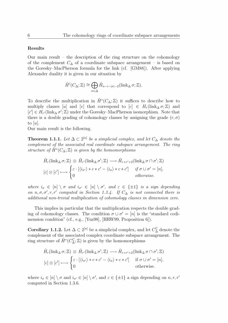
Our main result – the description of the ring structure on the cohomologyof the complement C∆ of a coordinate subspace arrangement – is based onthe Goresky–MacPherson formula for the link (cf. [GM88]). After applyingAlexander duality it is given in our situation by

H i(C∆; Z) ∼=⊕σ∈∆

Hn−i−|σ|−2(link∆ σ; Z).

To describe the multiplication in H∗(C∆; Z) it suffices to describe how tomultiply classes [u] and [v] that correspond to [c] ∈ Hr(link∆ σ; Z) and[c′] ∈ Hr′(link∆ σ′; Z) under the Goresky–MacPherson isomorphism. Note thatthere is a double grading of cohomology classes by assigning the grade (r, σ)to [u].Our main result is the following.

Theorem 1.1.1. Let ∆ ⊂ 2[n] be a simplicial complex, and let C∆ denote thecomplement of the associated real coordinate subspace arrangement. The ringstructure of H∗(C∆; Z) is given by the homomorphisms

Hr(link∆ σ; Z) ⊗ Hr′(link∆ σ′; Z) −→ Hr+r′+2(link∆ σ ∩ σ′; Z)

[c] ⊗ [c′] 7−→{

ε · [〈iσ′〉 ∗ c ∗ c′ − 〈iσ〉 ∗ c ∗ c′] if σ ∪ σ′ = [n],

0 otherwise.

where iσ ∈ [n] \ σ and iσ′ ∈ [n] \ σ′, and ε ∈ {±1} is a sign dependingon n, σ, σ′, r, r′ computed in Section 1.3.4. If C∆ is not connected there isadditional non-trivial multiplication of cohomology classes in dimension zero.

This implies in particular that the multiplication respects the double grad-ing of cohomology classes. The condition σ ∪ σ′ = [n] is the “standard codi-mension condition” (cf., e.g., [Yuz98], [HRW99, Proposition 6]).

Corollary 1.1.2. Let ∆ ⊂ 2[n] be a simplicial complex, and let CC∆ denote the

complement of the associated complex coordinate subspace arrangement. Thering structure of H∗(CC

∆; Z) is given by the homomorphisms

Hr(link∆ σ; Z) ⊗ Hr′(link∆ σ′; Z) −→ Hr+r′+2(link∆ σ ∩ σ′; Z)

[c] ⊗ [c′] 7−→{

ε · [〈iσ′〉 ∗ c ∗ c′ − 〈iσ〉 ∗ c ∗ c′] if σ ∪ σ′ = [n],

0 otherwise.

where iσ ∈ [n] \ σ and iσ′ ∈ [n] \ σ′, and ε ∈ {±1} a sign depending on n, r, r′

computed in Section 1.3.6.

1.2 Objects, Tools and Facts 7

The fact that the sign ε depends on σ and σ′ in the real case, but not inthe complex case, is the reason why in general there is no (dimension-shifting)isomorphism of graded rings between the cohomology rings of the real andcomplex arrangement associated with ∆ (compare Corollary 1.2.2 and Section1.4).

Example 1.1.3. There is a simplicial complex ∆ ⊂ 2[8] on eight vertices suchthat the following holds.

. The complement of the associated real arrangement is connected.

. The ring structure of H∗(C∆; Z) differs from H∗(CC∆; Z).

Example 1.1.4. There is a simplicial complex ∆ ⊂ 2[10] on ten vertices suchthat the cohomology ring of the complement of the associated real (or complex)arrangement yields non-trivial multiplication of torsion elements.

1.2 Objects, Tools and Facts

In this section we recall basic facts on coordinate subspace arrangements, pro-vide combinatorial models for their links and complements, and describe Lef-schetz duality in the framework of cubical cohomology for the complement ofa coordinate subspace arrangement.

1.2.1 Coordinate Subspace Arrangements

Simplicial complexes give rise to real and complex subspace arrangements.For that, let {e1, . . . , en} be the standard basis of Rn, resp. {eC

1 , . . . , eCn} the

standard basis of Cn. Let ∆ ⊂ 2[n] be a simplicial complex on the vertex set[n] = {1, . . . , n}. We define that always ∅ ∈ ∆ is a face. To avoid trivialcases we assume throughout this chapter that ∆ 6= 2[n] and n ≥ 2. The (real)coordinate subspace arrangement in Rn associated with ∆ is

A∆ = {spanR{ei0 , . . . , eik} : {i0, . . . , ik} ∈ ∆} ,

the (complex) coordinate subspace arrangement in Cn associated with ∆ is

AC∆ =

{spanC{eC

i0, . . . , eC

ik} : {i0, . . . , ik} ∈ ∆

}.

For every subspace arrangement we have the notion of the link and the com-plement, which in our case we denote by L∆ and C∆, resp. LC

∆ and CC∆.

L∆ = Sn−1 ∩⋃

A∆ C∆ = Rn \⋃

A∆

LC∆ = S2n−1 ∩

⋃AC

∆ CC∆ = Cn \

⋃AC

∆


1.2.2 Models for the Real Case

We introduce combinatorial models Λ∆ and Γ∆ for L∆ and C∆. Consider then-dimensional cross polytope Qn = conv{±ei : i = 1, . . . , n}. Its proper facesform a simplicial complex, which we denote by ∂Qn. Let Λ∆ be the subcomplexof ∂Qn of all simplices that are contained in

⋃A∆.

Λ∆ ={{ε0ei0 , . . . , εkeik} : {i0, . . . , ik} ∈ ∆, (ε0, . . . , εk) ∈ {±1}k+1

}Let Γ∆ be the “mirror complex” of A∆ (cf. [BBC97]), i.e., the faces of then-cube Cn = [−1, 1]n disjoint to

⋃A∆ considered as a polytopal subcomplexof the cube.

Γ∆ = {c : c a proper face of Cn, [n]\ {varying coord. of c} 6∈ ∆}

The underlying spaces |Λ∆| and |Γ∆| are homeomorphic, resp. homotopyequivalent, to the link L∆ and the complement C∆, see e.g. [Mun84, p. 414].

1.2.3 From Complex to Real Arrangements

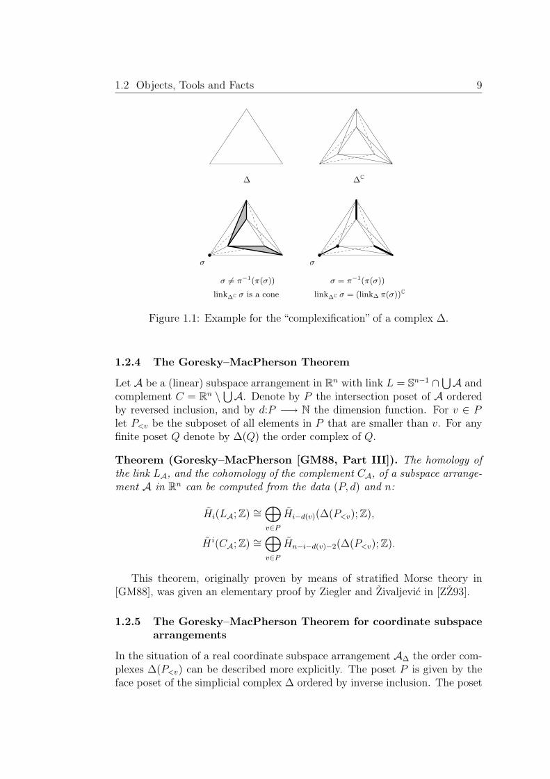
As far as the topology is concerned any complex coordinate arrangement canbe modeled as a real subspace arrangement. Let ∆ ⊂ 2[n] be a simplicialcomplex on the vertex set {1, . . . , n}. Let π : [2n] −→ [n] the map defined by2i − 1, 2i 7→ i for i ∈ [n]. Define the “complexification” of ∆ by

∆C = {σ ⊂ [2n] : π(σ) ∈ ∆}.

For an example of a “complexification” and the following Lemma see Figure1.1.

Lemma 1.2.1.

. Under the standard identification Cn ∼= R2n the spaces⋃AC

∆ and⋃A∆C

correspond to each other.

. For σ ∈ ∆C the following homotopy equivalence holds

link∆C σ '{∗ if π−1(π(σ)) 6= σ,

link∆ π(σ) if π−1(π(σ)) = σ.


σσ

∆ ∆C

link∆C σ is a cone

σ 6= π−1(π(σ)) σ = π−1(π(σ))

link∆C σ = (link∆ π(σ))C

Figure 1.1: Example for the “complexification” of a complex ∆.

1.2.4 The Goresky–MacPherson Theorem

Let A be a (linear) subspace arrangement in Rn with link L = Sn−1 ∩ ⋃A andcomplement C = Rn \ ⋃A. Denote by P the intersection poset of A orderedby reversed inclusion, and by d:P −→ N the dimension function. For v ∈ Plet P<v be the subposet of all elements in P that are smaller than v. For anyfinite poset Q denote by ∆(Q) the order complex of Q.

Theorem (Goresky–MacPherson [GM88, Part III]). The homology ofthe link LA, and the cohomology of the complement CA, of a subspace arrange-ment A in Rn can be computed from the data (P, d) and n:

Hi(LA; Z) ∼=⊕v∈P

Hi−d(v)(∆(P<v); Z),

H i(CA; Z) ∼=⊕v∈P

Hn−i−d(v)−2(∆(P<v); Z).

This theorem, originally proven by means of stratified Morse theory in[GM88], was given an elementary proof by Ziegler and Zivaljevic in [ZZ93].

1.2.5 The Goresky–MacPherson Theorem for coordinate subspacearrangements

In the situation of a real coordinate subspace arrangement A∆ the order com-plexes ∆(P<v) can be described more explicitly. The poset P is given by theface poset of the simplicial complex ∆ ordered by inverse inclusion. The poset


P<σ then is isomorphic to the opposite face lattice of link∆ σ = {τ ∈ ∆ :σ ∪ τ ∈ ∆, σ ∩ τ = ∅}. Thus we obtain the following formulation of theGoresky–MacPherson theorem.

Theorem. Let ∆ ⊂ 2[n] be a simplicial complex with vertex set {1, . . . , n}.Then

Hi(L∆; Z) ∼=⊕σ∈∆

Hi−|σ|(link∆ σ; Z),

H i(C∆; Z) ∼=⊕σ∈∆

Hn−i−|σ|−2(link∆ σ; Z).

Here |σ| denotes the cardinality of σ, i.e., |σ| = dim σ + 1.

In view of section 1.2.2 this yields the following result for the associatedcomplex coordinate subspace arrangement.

Corollary 1.2.2. For simplicial complexes ∆ ⊂ 2[n] we have

Hi

(LC

∆; Z) ∼=

⊕σ∈∆

Hi−2|σ|(link∆ σ; Z)

H i(CC

∆; Z) ∼=

⊕σ∈∆

H2n−i−2|σ|−2(link∆ σ; Z),

and hence there is a dimension-shifting group isomorphism between the(co)homologies of the real and complex coordinate subspace arrangements.Every homology class

[c] ∈ Hn−i−|σ|−2(link∆ σ; Z) = H2n−(n+|σ|+i)−2|σ|−2(link∆ σ; Z)

corresponds to

[u] ∈ H i(C∆; Z)

and to

[uC] ∈ Hn+|σ|+i(CC

∆; Z).

The correspondence [u] 7−→ [uC] sets up the isomorphism.

1.2.6 A Homology Model and a Map into the Link

We establish a simplicial version of the Ziegler–Zivaljevic [ZZ93] proof for theGoresky–MacPherson theorem. Let ∆ ⊂ 2[n] be a simplicial complex. Weconstruct a simplicial complex L∆ together with a simplicial map Φ : L∆ −→


Λ∆ to the link that induces an isomorphism in homology. Let L∆ be thefollowing one-point union of spaces.

L∆ =

( ⋃σ∈∆

∂Q|σ| ∗ link∆ σ

)/∼ =

∆ ∪⋃

σ∈∆\{∅}∂Q|σ| ∗ link∆ σ

/∼

The one-point union is given by the following identifications ∼. For eachσ = {i0 < . . . < ik} ∈ ∆, σ 6= ∅, identify e1 ∈ ∂Q|σ| ∗ link∆ σ with the vertexi0 ∈ ∆ = ∂Q|∅| ∗ link∆ ∅. Compare Figure 1.2.

��

��

��

��

��

��

��

��

��

��

��

��

��

��

��3′

2

3

2

2′′1 3

e1

e2

e3

1′

2′1

∆ Λ∆ L∆

Figure 1.2: An easy example for the model space L∆.

We get the map Φ by defining it on the pieces ∂Q|σ| ∗ link∆ σ. Let

φσ : ∂Q|σ| ∗ link∆ σ −→ Λ∆

be defined by the simplicial homeomorphism

∂Q|σ| −→ spanR{ei0 , . . . , eik} ∩ ∂Qn,

σ = {i0 < · · · < ik}, such that φσ(ej+1) = eij , in particular φσ(e1) = ei0 . Onlink∆ σ the map φσ is defined by

{j0, . . . , jl} 7−→ {ej0 , . . . , ejl} ∈ Λ∆

for {j0, . . . , jl} ∈ link∆ σ. By construction all these maps fit together and yielda simplicial map Φ.

Proposition 1.2.3. The map Φ induces an isomorphism in homology. (Infact, it is a homotopy equivalence.)

Sketch of proof. The proof works as in [ZZ93] by induction on the cardinalityof ∆. In the induction step one removes a maximal simplex of ∆ and usesthe Mayer-Vietoris sequence along with the induction hypotheses (resp. theGlueing Lemma, to obtain the homotopy equivalence).


1.2.7 Cubical Cohomology

The homotopy model Γ∆ of the complement C∆ is a subcomplex of the bound-ary of the cube. We compute its cohomology by using “cubical cohomology.”We give a short overview of the most important notation and the formula forthe cup product (see also [Mas91]).Let Γ be a subcomplex of the n-cube Cn, and let T ∈ Γ be a t-dimensionalcube. We use two descriptions of T :Denote the projection to the i-th coordinate by πi. On the one hand, we canidentify T with a vector in {+,−, ∗}n, where the i-th coordinate is +, − or ∗iff πi(T ) = {+1}, {−1}, resp. [−1, +1]. On the other hand, there are threesets T+, T−, T∗ ⊆ {1, . . . , n} that uniquely define the cube,

T1−1! (T+, T−, T∗),

where |T∗| = t and the following holds for the coordinate projections.

πi(T ) = {+1} for i ∈ T+,

πj(T ) = {−1} for j ∈ T−,

πk(T ) = [−1, +1] for k ∈ T∗.

Let Ct(Γ) be the free abelian group generated by the t-cubes in Γ. In orderto get a boundary map we begin by defining face operators. Let T ∈ Γ be

a t-dimensional cube T1−1! (T+, T−, T∗) with T∗ = {k1 < · · · < kt}. For A =

{a1, . . . , ap} ⊆ {1, . . . , t} and ε = ±1 define the (t − p)-cube

DεAT =

{(T+ ∪ {ka1 , . . . , kap}, T−, T∗ \ {ka1 , . . . , kap}) if ε = +1,

(T+, T− ∪ {ka1 , . . . , kap}, T∗ \ {ka1 , . . . , kap}) if ε = −1.

DεAT is the face of T obtained by fixing the varying coordinates {ka1 , . . . , kap}

to ε. A boundary operator is now defined by

∂t : Ct(Γ) −→ Ct−1(Γ),

T 7−→t∑

a=1

(−1)a(D+1

{a}T − D−1{a}T

).

The homology of the resulting cubical chain complex (C∗(Γ), ∂∗) is canonicallyisomorphic to singular homology. The cup product formula in this situationis given on the chain level by the following. Let u ∈ Hom(Cp(Γ), Z) andv ∈ Hom(Cq(Γ), Z), then for a (p + q)-cube T we obtain

(u ∪ v)(T ) =∑

ρH,K · u (D+1

H T)v

(D−1

K T),

where the sum is taken over all q-subsets H of {1, . . . , p + q}, K is the com-plement of H, and ρH,K is the sign of the permutation HK of {1, . . . , p + q},i.e., the signature of the shuffle (H,K).


1.2.8 Lefschetz Duality for the Cross Polytope

As a crucial part of Alexander duality, we describe Lefschetz duality explicitlyfor simplicial homology of the cross polytope and cubical cohomology of thecube (cf. [Mun84]).

Theorem (Lefschetz Duality). Let (X,A) be a compact, orientable, trian-gulated relative homology n-manifold. Then there is an isomorphism

Hk(X,A) ∼= Hn−k(|X| \ |A|).

Outline of the proof. Let X− be the simplicial complex consisting of all sim-plices of the barycentric subdivision sdX that are disjoint from |A|. Then

. |X−| is a deformation retract of |X| \ |A|.

. |X−| equals the union of all blocks D(σ) dual to simplices σ ∈ X thatare not in A.

Now there is a chain isomorphism

Ck(X,A)∼=−→ Dn−k(X

−),

where D∗(X−) denotes the dual chain complex of X−. Dualization yields

Ck(X,A) ∼= Hom(Ck(X,A), Z)∼=←− Hom(Dn−k(X

−), Z).

The inverse map Ck(X,A) −→ Hom(Dn−k(X−), Z) is given by σ 7→ D(σ)∗,

where σ is a k-simplex of X not in A. This induces the desired isomorphism.

Lefschetz duality is dealing with the complex X−, whose underlying spaceis the union of the dual blocks D(σ), σ ∈ X \A. In case X is the boundary ofthe cross polytope Qn, the dual blocks |D(σ)|, σ ∈ X, correspond to the facesof the boundary of the n-dimensional cube Cn. See Figure 1.3.

Let now A = Λ∆ be the subcomplex of X = ∂Qn given by the arrange-ment associated with a simplicial complex ∆ (Section 1.2.2). Then there is achain isomorphism from the dual block complex of (∂Qn)− to the cubical chaincomplex of Γ∆

Dj((∂Qn)−) −→ Cj(Γ∆),

which yields a chain isomorphism

Ψ : Ck(∂Qn, Λ∆) −→ Hom(Dn−1−k((∂Qn)−), Z) −→ Hom(Cn−1−k(Γ∆), Z)


Figure 1.3: The 3-dimensional cross polytope with the 1-skeleton of the 3-dimensional cube in the barycentric subdivision.

where

Ψ(σ) = (−1)i0+···+ik(−1)|T−(σ)|(T+(σ), T−(σ), T∗(σ))∗,

for σ = 〈ε0ei0 , . . . , εkeik〉 ∈ ∂Qn \ Λ∆, i0 < · · · < ik, with

T+(σ) = {ij ∈ [n] : εj = +1},T−(σ) = {ij ∈ [n] : εj = −1},T∗(σ) = [n] \ (T+(σ) ∪ T−(σ)).

The signs in Ψ(σ) result from the condition that Ψ must commute with therespective boundary maps.

1.3 Proofs of Results

In this section we prove Theorem 1.1.1. We begin by introducing joins ofchains, and then exhibit explicit cohomology classes in H∗(Γ∆) with respectto the Goresky–MacPherson theorem. We derive an explicit formula for thecup product of two such classes. In most of the cases the product vanishes asstated in Theorem 1.1.1. Then we treat the case in which the product doesnot vanish. The considerations of the complex case follow then.

1.3 Proofs of Results 15

1.3.1 Joins of Chains

Definition 1.3.1. The join c ∗ c′ of two simplicial chains c =∑

j αjτj and

c′ =∑

k α′kτ

′k in a simplicial complex ∆ ⊂ 2[n] is defined by

∑j,k

τj∩τ ′k=∅

αjα′k τj ∗ τ ′

k,

where the join of two disjoint oriented simplices is defined by

〈v0, . . . , vr〉 ∗ 〈w0, . . . , ws〉 = 〈v0, . . . , vr, w0, . . . , ws〉.

Lemma 1.3.2. Let R = {r0, . . . , rs} be a subset of the vertex set, c =∑

j αjτj

a cycle. For R ⊂ τj define the (oriented) simplex τj by the equation τj =τj ∗ 〈r0, . . . , rs〉. Then

∑j:R⊂τj

αj τj is a cycle.

Proof. We write c as

c =∑

j:R 6⊂τj

αjτj +∑

j:R⊂τj

αj τj ∗ 〈r0, . . . , rs〉,

and obtain for the boundary

∂

∑j:R 6⊂τj

αjτj

+ ∂

∑j:R⊂τj

αj τj

∗ 〈r0, . . . , rs〉

±∑

j:R⊂τj

αj τj ∗ ∂(〈r0, . . . , rs〉) = 0.

The only simplices that contain R appear in the second summand, and hencethis summand must be zero on its own.

Lemma 1.3.3. Let i be a vertex and let c =∑

j αjτj and c′ =∑

k α′kτ

′k be

two cycles that share at most the vertex i. Then

∂(〈i〉 ∗ c ∗ c′) = c ∗ c′.


Proof.

∂(〈i〉 ∗ c ∗ c′) = ∂

〈i〉 ∗∑j:i6∈τj

αjτj ∗∑

k:i6∈τ ′k

α′kτ

′k

=

∑j:i6∈τj

αjτj ∗∑

k:i6∈τ ′k

α′kτ

′k − 〈i〉 ∗ ∂

∑j:i6∈τj

αjτj

∗∑

k:i6∈τ ′k

α′kτ

′k

± 〈i〉 ∗∑j:i6∈τj

αjτj ∗ ∂

∑k:i6∈τ ′

k

α′kτ

′k

=

∑j:i6∈τj

αjτj ∗∑

k:i6∈τ ′k

α′kτ

′k + 〈i〉 ∗ ∂

∑j:i∈τj

αjτj

∗∑

k:i6∈τ ′k

α′kτ

′k

± 〈i〉 ∗∑j:i6∈τj

αjτj ∗ ∂

∑k:i6∈τ ′

k

α′kτ

′k

= c ∗

∑k:i6∈τ ′

k

α′kτ

′k −

∑j:i6∈τj

αjτj ∗ 〈i〉 ∗ ∂

∑k:i6∈τ ′

k

α′kτ

′k

= c ∗

∑k:i6∈τ ′

k

α′kτ

′k +

∑j:i6∈τj

αjτj ∗ 〈i〉 ∗ ∂

∑k:i∈τ ′

k

α′kτ

′k

= c ∗ c′,

where possible empty sums are considered to be zero.

1.3.2 Explicit Cocycles

Using the Goresky–MacPherson theorem and the explicit description ofAlexander duality we now derive explicit cohomology cocycles for the com-plement of a coordinate subspace arrangement. For that, we use the followingsequence of homomorphisms.

Hr(link∆ σ)∼=−−−−−−→

suspensionHr+|σ|

(∂Q|σ| ∗ link∆ σ

) ↪→−−−→(φσ)∗

Hr+|σ|(Λ∆)

−−−−−−−→pair sequence

Hr+|σ|+1(∂Qn, Λ∆)∼=−−−−−−−−−→

Lefschetz dualityHn−r−|σ|−2(Γ∆) (1.1)

Before describing the maps explicitly, we introduce some notation.

Notation 1.3.4. . For each subset {j1, . . . , js} ⊂ [n] we define

sign(j1j2 · · · js) = sign π,


where π is the permutation of (1, . . . , s) such that jπ(1) < · · · < jπ(s). Forevery family of subsets A1, . . . , Ak ⊂ [n], where Ai = {ji

1 < · · · < jimi},

we define

sign(A1 · · ·Ak) = sign(j11 , . . . , j

1m1

, j21 , . . . , j

2m2

, . . . , jk1 , . . . , jk

mk).

Furthermore, for every set A = {a1, . . . , ak} ⊂ [n] we abbreviate(−1)a1+···+an by (−1)ΣA.

. For each σ ∈ ∆ let

sσ =∑

~ε=(ε0,...,εk)∈{±1}k+1

ε0 · · · εk · 〈ε0e0, . . . , εkek〉

be a generating simplicial cycle of H|σ|−1(∂Q|σ|).

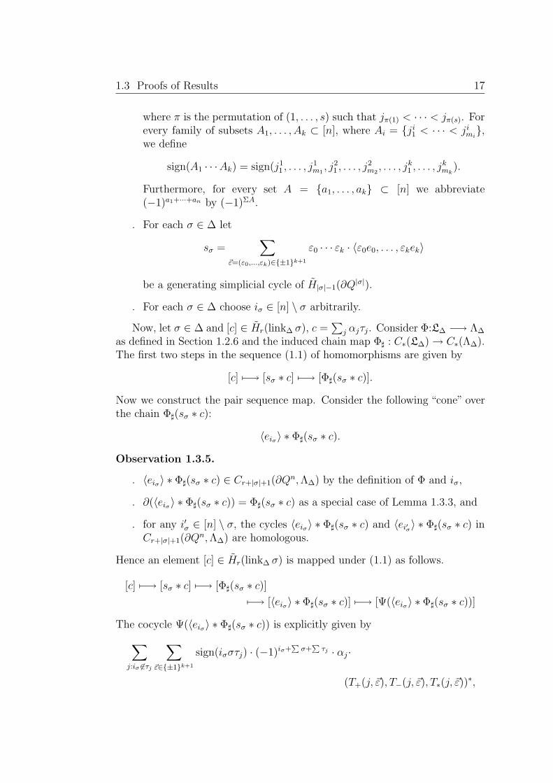
. For each σ ∈ ∆ choose iσ ∈ [n] \ σ arbitrarily.

Now, let σ ∈ ∆ and [c] ∈ Hr(link∆ σ), c =∑

j αjτj. Consider Φ:L∆ −→ Λ∆

as defined in Section 1.2.6 and the induced chain map Φ] : C∗(L∆) → C∗(Λ∆).The first two steps in the sequence (1.1) of homomorphisms are given by

[c] 7−→ [sσ ∗ c] 7−→ [Φ](sσ ∗ c)].

Now we construct the pair sequence map. Consider the following “cone” overthe chain Φ](sσ ∗ c):

〈eiσ〉 ∗ Φ](sσ ∗ c).

Observation 1.3.5.

. 〈eiσ〉 ∗ Φ](sσ ∗ c) ∈ Cr+|σ|+1(∂Qn, Λ∆) by the definition of Φ and iσ,

. ∂(〈eiσ〉 ∗ Φ](sσ ∗ c)) = Φ](sσ ∗ c) as a special case of Lemma 1.3.3, and

. for any i′σ ∈ [n] \ σ, the cycles 〈eiσ〉 ∗ Φ](sσ ∗ c) and 〈ei′σ〉 ∗ Φ](sσ ∗ c) inCr+|σ|+1(∂Qn, Λ∆) are homologous.

Hence an element [c] ∈ Hr(link∆ σ) is mapped under (1.1) as follows.

[c] 7−→ [sσ ∗ c] 7−→ [Φ](sσ ∗ c)]

7−→ [〈eiσ〉 ∗ Φ](sσ ∗ c)] 7−→ [Ψ(〈eiσ〉 ∗ Φ](sσ ∗ c))]

The cocycle Ψ(〈eiσ〉 ∗ Φ](sσ ∗ c)) is explicitly given by∑j:iσ 6∈τj

∑~ε∈{±1}k+1

sign(iσστj) · (−1)iσ+∑

σ+∑

τj · αj·

(T+(j, ~ε), T−(j, ~ε), T∗(j, ~ε))∗,


where

T+(j, ~ε) = τj ∪ {iσ} ∪ {il : εl = +1},T−(j, ~ε) = {il : εl = −1},T∗(j, ~ε) = [n] \ (T+(j, ~ε) ∪ T−(j, ~ε))

= [n] \ (σ ∪ τj ∪ {iσ}).

Here we made use of the equality ε0 · · · εk · (−1)|T−(j,~ε)| = +1. In the otherrepresentation the cubes (T+(j, ~ε), T−(j, ~ε), T∗(j, ~ε)) look as in Figure 1.4 (upto a permutation of coordinates), where the ±-signs correspond to the signvector ~ε.

(±±±±±±±±± ∗ ∗ ∗ ∗ + ∗ ∗ ∗ ∗ ∗ + + + + ∗ ) ,︸︷︷︸σ

︸︷︷︸{iσ}

︸︷︷︸τj

Figure 1.4: Schematic description of (T+(j, ~ε), T−(j, ~ε), T∗(j, ~ε)).

Throughout the rest of the chapter we will use this correspondence be-tween homology cycles of the links of ∆ and cocycles of the complement of thearrangement.

1.3.3 The Cup Product

Now consider two cohomology classes [u] and [v] of Γ∆ corresponding to twohomology classes [c] ∈ Hr(link∆ σ) and [c′] ∈ Hr′(link∆ σ′) for simplices σ, σ′ ∈∆, c =

∑j αjτj and c′ =

∑k α′

kτ′k. Let p = n−r−|σ|−2 and q = n−r′−|σ′|−2

and let T ∈ Γ∆ be a (p+ q)-cube. For the cup product of [u] and [v] evaluatedat T we obtain∑

H,K

∑j:iσ 6∈τj

k:iσ′ 6∈τ ′k

∑~ε,~ε ′

ρH,K sign(iσστj) sign(iσ′σ′τ ′k) · (−1)iσ+iσ′+

∑σ+

∑τj+

∑σ′+

∑τ ′k ·

αjα′k · (T+(j, ~ε), T−(j, ~ε), T∗(j, ~ε))∗(D+1

H T )·(T ′

+(k, ~ε ′), T ′−(k, ~ε ′), T ′

∗(k, ~ε ′))∗(D−1K T ),

where the first summation is over all (q, p)-shuffles (H,K). Let us first consideronly the last term

(T+(j, ~ε), T−(j, ~ε), T∗(j, ~ε))∗(D+1H T )·

(T ′+(k, ~ε ′), T ′

−(k, ~ε ′), T ′∗(k, ~ε ′))∗(D−1

K T ). (∗)


Observation 1.3.6. The term (∗) vanishes for all H,K and ~ε, ~ε ′ unless

σ ∪ σ′ ∪ {iσ} ∪ {iσ′} ∪ τj ∪ τ ′k = [n].

Proof. The sets of varying coordinates in D+1H T and D−1

K T are disjoint. Thisgives

∅ = T∗(j, ~ε) ∩ T ′∗(k, ~ε ′)

= ([n] \ (σ ∪ τj ∪ {iσ})) ∩ ([n] \ (σ′ ∪ τ ′k ∪ {iσ′})),

which yields the result.

Now we turn to the general computation of the cup product.Case I: σ 6= σ′ and σ ∪ σ′ 6= [n].In this case we will show that the cup product vanishes as demanded in thestatement of the main Theorem. By anti-commutativity of the cup product wemay assume σ′ 6⊂ σ. By Observation 1.3.5 we can assume iσ = iσ′ 6∈ [n]\(σ∪σ′).Our situation is represented in Figure 1.5.

τj∩σ′︷︸︸︷ σ︷︸︸︷ ↓τj\σ′︷︸︸︷ iσ︷︸︸︷

( ∗ ∗ + + + + ∗ ∗ ∗ ∗ ∗ ±±±±±± ∗ ∗ ∗ + + + + )∗(D+1H T )·

(±±±±± ± ±±±±±±±± ∗ ∗ + + + + + ∗ ∗ + )∗(D−1K T )︸︷︷︸

σ′︸︷︷︸

τ ′k

︸︷︷︸iσ′

(∗ ∗ + + + + ∗ ∗ ∗ ∗ ∗ ±±± ∗ ∗ + ∗ ∗ ∗ + ∗ ∗ + )

Figure 1.5: The term (∗) schematically and all cubes T for which (∗) has achance not to vanish.

Observation 1.3.7. The term (∗) vanishes for all H,K, ~ε, ~ε ′, and k unlessthe following holds

σ ∪ σ′ ∪ {iσ} ∪ τj = [n].

Proof. As the down arrow ↓ points out in Figure 1.5, if there is a coordinateonly covered by τ ′

k it will be a fixed −1-coordinate in D−1K T .

Hence all terms that have a chance to contribute to a non trivial productare as shown in Figure 1.6.


τj∩σ′︷︸︸︷ σ︷︸︸︷ τj\σ′︷︸︸︷ iσ︷︸︸︷( ∗ ∗ + + + + ∗ ∗ ∗ ∗ ∗ ±±±±±±+ + + + + + + )∗(D+1

H T )·(±±±±± ± ±±±±±±±± ∗ ∗ + + + + + ∗ ∗ + )∗(D−1

K T )︸︷︷︸σ′

︸︷︷︸τ ′k

︸︷︷︸iσ′

(∗ ∗ + + + + ∗ ∗ ∗ ∗ ∗ ±±± ∗ ∗ + + + + + ∗ ∗ + )

Figure 1.6: The term (∗) schematically and all cubes T contributing non zerosummands.

Gathering all contributing terms with the right sign and coefficient, weobtain that the cup product is represented by the following cocycle (up to aglobal sign)

Ψ

〈eiσ〉 ∗ Φ]

sσ∩σ′ ∗∑

j:iσ 6∈τj

R⊂τj

αj τj ∗∑

k:iσ 6∈τ ′k

α′kτ

′k

,

where R = {r0, . . . , rs} = [n]\ (σ∪σ′∪{iσ}) and τj = τj ∗ 〈r0, . . . , rs〉. Tracingthis element back through the sequence of homomorphisms in (1.1) and usingLemma 1.3.3 we arrive (up to a global sign) at

∂

〈iσ〉 ∗∑

j:iσ 6∈τj

R⊂τj

αj τj ∗∑

k:iσ 6∈τ ′k

α′kτ

′k

=∑

jR⊂τj

αj τj ∗ c′

as a representing cycle in H∗(link∆(σ ∩ σ′)), which we denote by c ∗ c′. Thisis a chain in Ck(link∆(σ ∩ σ′)) for the following reason. Consider an arbitrarypair of simplices τj and τ ′

k. Since τ ′k ∈ link∆ σ′ we have σ′ ∪ τ ′

k ∈ ∆ and sinceτj ⊂ σ′ we obtain τj ∪ τ ′

k ∈ ∆.We claim that the cycle c ∗ c′ is a boundary in Ck(link∆(σ ∩ σ′)). Since σ′ 6⊂ σthere is a p ∈ σ′ \ σ and as before all simplices {p} ∪ τj ∪ τ ′

k ∈ ∆. Hence〈p〉 ∗ c ∗ c′ ∈ Ck+1(link∆(σ ∩ σ′)) with boundary c ∗ c′ as follows by Lemma1.3.3.Case II: σ = σ′ (of course σ 6= [n]). We will show that the cup productvanishes unless the complement C∆ is not connected. In this case we get non-trivial self multiplication of elements in cohomological dimension 0. Again wecan assume iσ = iσ′ . Our situation is shown in Figure 1.7.


σ︷︸︸︷ ↓τj︷︸︸︷ iσ︷︸︸︷

(±±±±±±±±±±±±±±±±± ∗ ∗ + + + + + )∗(D+1H T )·

(±±±±±±±±±±±±±±±±±+ + + + ∗ ∗ + )∗(D−1K T )︸︷︷︸

σ′︸︷︷︸

τ ′k

︸︷︷︸iσ′

(±±±±±±±±±±±±±±±±± ∗ ∗ + + ∗ ∗ + )

Figure 1.7: The term (∗) schematically and all possible cubes T on which itdoes not vanish.

As in the last case (↓) the only interesting terms are the ones with σ ∪τj ∪ {iσ} = [n]. If such a term exists c must be a multiple of a generatingcycle of the sphere on the vertices [n] \ σ. But for c′ not to be trivial the sameholds for c′, since the reduced homology of the sphere is non trivial only in thedimension of the sphere. Now n−|σ|− r− 2 = n−|σ′|− r′− 2 = 0. Thereforethe corresponding cohomology classes are not zero only if C∆ is not connected,which means that there are simplices of dimension n − 2 in ∆.Case III: σ ∪ σ′ = [n]. Consider Figure 1.8.

τj︷︸︸︷ iσ︷︸︸︷ σ︷︸︸︷( ∗ ∗ + + + + ∗ ∗ + ∗ ∗ ±±±±±±±±± ± ±± ± )∗(D+1

H T )·(±±±±± ± ±± ± ±±±±± ∗ ∗ + + + + + ∗ ∗ + )∗(D−1

K T )︸︷︷︸σ′

︸︷︷︸τ ′k

︸︷︷︸iσ′

(∗ ∗ + + + + ∗ ∗ + ∗ ∗ ±±± ∗ ∗ + + + + + ∗ ∗ + )

Figure 1.8: The term (∗) schematically and all cubes T for which (∗) does notvanish.

Gathering the cocubes corresponding to the non vanishing summands to-gether with signs and coefficients gives the following representing cocycle forthe cup product (up to a global sign, see Section 1.3.4)

Ψ

〈eiσ〉 ∗ 〈eiσ′ 〉 ∗ Φ]

sσ∩σ′ ∗∑

j:iσ 6∈τj

αjτj ∗∑


α′kτ

′k

.


Tracing this element back to a cycle in Cr+r′+2(link∆(σ ∩ σ′)) leads up to afactor of (−1)|σ∩σ′| to

∂

〈iσ〉 ∗ 〈iσ′〉 ∗∑

j:iσ 6∈τj

αjτj ∗∑


α′kτ

′k

=

= 〈iσ′〉 ∗∑

j:iσ 6∈τj

αjτj ∗∑


α′kτ

′k − 〈iσ〉 ∗

∑j:iσ 6∈τj

αjτj ∗∑


α′kτ

′k

− 〈iσ′〉 ∗ 〈iσ〉 ∗ ∂

∑j:iσ 6∈τj

αjτj

∗∑


α′kτ

′k

+ 〈iσ〉 ∗∑

j:iσ 6∈τj

αjτj ∗ 〈iσ′〉 ∗ ∂

∑k:iσ′ 6∈τ ′

k

α′kτ

′k

= 〈iσ′〉 ∗

∑j:iσ 6∈τj

αjτj ∗∑


α′kτ

′k − 〈iσ〉 ∗

∑j:iσ 6∈τj

αjτj ∗∑


α′kτ

′k

+ 〈iσ′〉 ∗ 〈iσ〉 ∗ ∂

∑j:iσ∈τj

αjτj

∗∑


α′kτ

′k

− 〈iσ〉 ∗∑

j:iσ 6∈τj

αjτj ∗ 〈iσ′〉 ∗ ∂

∑k:iσ′∈τ ′

k

α′kτ

′k

= 〈iσ′〉 ∗ c ∗

∑k:iσ′ 6∈τ ′

k

α′kτ

′k − 〈iσ〉 ∗

∑j:iσ 6∈τj

αjτj ∗ c′

= 〈iσ′〉 ∗ c ∗ c′ − 〈iσ〉 ∗ c ∗ c′.

This finishes the proof of Theorem 1.1.1.

1.3.4 The Global Sign

We show how to compute the global sign. In the cup product formula we havethe sign

ρH,K sign(iσστj) sign(iσ′σ′τ ′k) · (−1)iσ+iσ′+

∑σ+

∑τj+

∑σ′+

∑τ ′k . (∗)

For the image of 〈iσ′〉∗c∗c′−〈iσ〉∗c∗c′ under the sequence of homomorphisms(1.1) we obtain

(−1)|σ∩σ′| · Ψ〈eiσ〉 ∗ 〈eiσ′ 〉 ∗ Φ]

sσ∩σ′ ∗∑

j:iσ 6∈τj

αjτj ∗∑


α′kτ

′k

.


In this sum the sign of the cube in question is

(−1)|σ∩σ′| · sign(iσiσ′(σ ∩ σ′)τjτ′k) · (−1)iσ+iσ′+

∑(σ∩σ′)+

∑τj+

∑τ ′k . (∗∗)

The global sign is given by the quotient of the two signs (∗) and (∗∗).

(−1)|σ∩σ′| · ρH,K sign(iσστj) · sign(iσ′σ′τ ′k) · sign(iσiσ′(σ ∩ σ′)τjτ

′k)·

(−1)iσ+iσ′+∑

σ+∑

τj+∑

σ′+∑

τ ′k · (−1)iσ+iσ′+

∑(σ∩σ′)+

∑τj+

∑τ ′k

= (−1)|σ∩σ′|+∑(σ∪σ′) · ρH,K sign(iσστj) · sign(iσ′σ′τ ′

k)·sign(iσiσ′(σ ∩ σ′)τjτ

′k),

where

H = [n] \ (σ′ ∪ τ ′k ∪ {iσ′})

K = [n] \ (σ ∪ τj ∪ {iσ}).We will derive a formula that is easier to handle and, in particular, shows theindependence of j, k and iσ, iσ′ .

Lemma 1.3.8. Let σ, σ′ ⊂ [n] such that σ ∪ σ′ = [n], and ι = {i} ⊂ [n] \ σ,ι′ = {i′} ⊂ [n]\σ′, and r, r′ ≥ 0. Then for τ ⊂ [n]\(σ∪ι) and τ ′ ⊂ [n]\(σ′∪ι′)of cardinality r, resp. r′ we have

sign(([n] \ (σ′ ∪ τ ′ ∪ ι′))([n] \ (σ ∪ τ ∪ ι)))·sign(ιστ) sign(ι′σ′τ ′) sign(ιι′(σ ∩ σ′)ττ ′)

= (−1)rr′+r′(n−|σ|−1)+1 sign(([n] \ σ′)([n] \ σ)).

Note that for simplicity we have used r, r′ for the cardinalities of τ, τ ′ insteadof the dimensions.

Proof. We proceed in two steps. First we show, what happens if we reduce(r, r′) in the lexicographic order.For (r, r′) = (0, 0), we just have

sign(([n] \ (σ′ ∪ ι′))([n] \ (σ ∪ ι))) · sign(ισ) sign(ι′σ′) sign(ιι′(σ ∩ σ′)). (1.2)

Now assume r = 0 and r′ > 0. Choose two r′-sets τ ′1, τ

′2 ⊂ [n] \ (σ′ ∪ ι′), and

choose elements v1 ∈ τ ′1, v2 ∈ τ ′

2. Let τ ′1 = τ1 \ {v1} and τ ′

2 = τ ′2 \ {v2}. Then

sign(([n] \ (σ′ ∪ τ ′1/2 ∪ ι′))([n] \ (σ ∪ ι)))

= sign([n] \ (σ′ ∪ τ ′1/2 ∪ ι′)[n] \ (σ ∪ ι))(−1)|{a∈[n]\(σ∪ι):a<v1/2}|,

sign(ι′σ′τ ′1/2) = sign(ι′σ′τ ′

1/2)(−1)|{a∈ι′∪σ′:a>v1/2}|,

sign(ιι′(σ ∩ σ′)τ ′1/2) = sign(ιι′(σ ∩ σ′)τ ′

1/2)(−1)|{a∈ι∪ι′∪(σ∩σ′):a>v1/2}|.


Consider the sum of the (−1)-exponents.

|{a ∈ [n] \ (σ ∪ ι) : a < v1/2}| + |{a ∈ ι′ ∪ σ′ : a > v1/2}|+|{a ∈ ι ∪ ι′ ∪ (σ ∩ σ′) : a > v1/2}|

≡ |[n] \ (ι ∪ σ)| − |{a ∈ [n] \ (σ ∪ ι) : a > v1/2}|+|{a ∈ σ′ : a > v1/2}| + |{a ∈ ι ∪ (σ ∩ σ′) : a > v1/2}|

≡ |[n] \ (ι ∪ σ)| + |{a ∈ σ′ : a > v1/2}|+|{a ∈ [n] \ (σ ∪ ι) : a > v1/2}| + |{a ∈ ι ∪ (σ ∩ σ′) : a > v1/2}|

≡ |[n] \ (ι ∪ σ)| + 2|{a ∈ σ′ : a > v1/2}|≡ |[n] \ (ι ∪ σ)| (mod 2).

Hence, for reducing r′ by one we obtain a factor of (−1)n−|σ|−1 and thus intotal a factor (−1)r′(n−|σ|−1).Assume r > 0. This case works analogously, reducing two choices of r-setsτ1/2. In each step one gets a factor (−1)r′ . Hence, after r steps, we obtain afactor (−1)rr′ .Treating the expression (1.2) similarly yields

(−1) · sign(([n] \ σ′)([n] \ σ)),

which gives the result.

Thus, we derived the following global sign

(−1)n(n+1)

2+|σ∩σ′|+(r+1)(r′+1)+(r′+1)(n−|σ|−1)+1 · sign(([n] \ σ′)([n] \ σ))

= (−1)n(n+1)

2+|σ∩σ′|+(r′+1)(n+|σ|+r)+1 · sign(([n] \ σ′)([n] \ σ)). (1.3)

1.3.5 The Complex Case

We will explicitly compute the multiplication in H∗(CC∆; Z) using the results

and notation of Section 1.2.3 and the previous Section. Let [u], [v] ∈ H∗(CC∆; Z)

correspond to

[c] ∈ Hr(link∆ σ) ∼= Hr(link∆C π−1(σ))

and

[c′] ∈ Hr′(link∆ σ′) ∼= Hr′(link∆C π−1(σ′))

for simplices σ, σ′ ∈ ∆.Case I: If σ∪σ′ 6= [n] then π−1(σ)∪π−1(σ′) 6= [2n] and hence the cup productof [u] and [v] is zero.Case II: If σ = σ′ 6= [n] the cup product vanishes since the complement of a


complex coordinate subspace arrangement is connected.Case III: Now let σ ∪ σ′ = [n]. Consider the isomorphism

Hr(link∆ σ) −→ Hr(link∆C π−1(σ))

[c] 7−→ [cC]

induced by the vertex map i 7→ 2i − 1. It corresponds to the isomorphisminduced by the homotopy equivalence. Using this isomorphism for the cupproduct computation we are in the well known situation as shown in Figure1.9.

τCj︷︸︸︷ iCσ︷︸︸︷ π−1(σ)︷︸︸︷

( ∗ ∗ + + + + ∗ ∗ + ∗ ∗ ∗ ±±±±±±± ± ±±± ± )∗(D+1H T )·

(±±±±± ± ±± ± ±±±±± ∗ ∗ + + + + ∗ ∗ ∗ + )∗(D−1K T )︸︷︷︸

π−1(σ′)︸︷︷︸

τ ′k

C︸︷︷︸

iCσ′

(∗ ∗ + + + + ∗ ∗ + ∗ ∗ ∗ ±± ∗ ∗ + + + + ∗ ∗ ∗ + )

Figure 1.9: A typical summand of the cup product evaluated at T schematicallyand the cubes T for which it does not vanish.

Collecting all summands yields the cocycle

Ψ

〈eiσ〉 ∗ 〈eiσ′ 〉 ∗ Φ]

sπ−1(σ)∩π−1(σ′) ∗∑

j:iσ 6∈τCj

αjτCj ∗

∑k:iσ′ 6∈τ ′

kC

α′kτ

′k

C

for vertices iσ ∈ [2n] \ π−1(σ) and iσ′ ∈ [2n] \ π−1(σ′). As above this leads (upto the global sign) to

[〈iσ′〉 ∗ c ∗ c′ − 〈iσ〉 ∗ c ∗ c′] ∈ Hr+r′+2(link∆ σ ∩ σ′)∼= Hr+r′+2(link∆C π−1(σ ∩ σ′))

= Hr+r′+2(link∆C π−1(σ) ∩ π−1(σ′)).

1.3.6 The Global Sign in the Complex Case

First of all, from the computation in the real case, we obtain the sign

(−1)n(2n+1)+|π−1(σ)∩π−1(σ′)|+(r+1)(r′+1)+(r′+1)(2n−|π−1(σ)|−1)+1·sign(([2n] \ π−1(σ′))([2n] \ π−1(σ))).


Now in π−1(σ), π−1(σ′) resp., all elements appear in pairs. This simplifies thesign to

(−1)n+r(r′+1)+1. (1.4)

1.4 Example of a Simplicial Complex yielding differentRing Structures

Let [u], [v], [w] be cohomology classes of the complement of a real coordinatesubspace arrangement corresponding to homology classes of links of ∆, suchthat [u] ∪ [v] = [w]. Then our results imply that for the corresponding coho-mology classes of the complement of the associated complex arrangement wehave (see Corollary 1.2.2) [

uC] ∪ [vC]

= ± [wC]

.

Hence it arises the question if we can choose signs in the correspondence [u] 7→[uC] consistently such that it becomes a (dimension-shifting) ring isomorphism.An example of different ring structures containing hyperplanes was given in[GPW98]: the existence of hyperplanes lead to additional multiplication inthe real case. Our example shows that this is not the only case where non-isomorphic rings occur.

Remark 1.4.1. There is a (dimension shifting) ring isomorphism ofH∗(C∆; Z2) and H∗(CC

∆; Z2).

1.4.1 The Example: Different Sign Patterns

We construct a simplicial complex ∆ ⊂ 2[8] on eight vertices given by fourfacets σ1, σ2, σ

′1, σ

′2, and investigate the multiplication of cohomology classes

stemming from the links of these facets in the case of the associated real andcomplex arrangement. For the real and complex case the resulting sign patternimplies that there is no ring isomorphism between H∗(C∆) and H∗(CC

∆). Thefacets are given by the following scheme which also helps for computing thesigns appearing in the multiplication. A black box in position (ρ, j) indicatesthat j ∈ ρ.

1 2 3 4 5 6 7 8

σ1

σ2

σ′1

σ′2

Figure 1.10: The facets of ∆.

1.5 Example of non trivial multiplication of Torsion Elements 27

The sign patterns arising in the real and in the complex case according to(1.3) and (1.4) are given by the following table.

Sign (1.3) Sign (1.4)σ1 σ′

1 −1 −1σ1 σ′

2 −1 −1σ2 σ′

1 +1 −1σ2 σ′

2 −1 −1

Clearly, there is no consistent way of assigning signs in the correspondence[u] 7→ [uC].

1.5 Example of non trivial multiplication of Torsion El-ements

We construct a simplicial complex ∆ ⊂ 2[10]. Let σ := {1, 2, 3, 4, 5, 6} andP ⊂ 2{1,2,3,4,5,6} be a six-vertex triangulation of the projective plane. Let σ′ ={7, 8, 9, 10}, and let S be a simplicial 1-sphere on four vertices as a subcomplexof 2{7,8,9,10}. Now define ∆ = P ∗ 2σ′ ∪ 2σ ∗S. Then the homotopy type of ∆ isΣ(P ∗ 2σ′ ∩ 2σ ∗ S) = Σ(P ∗ S). Hence ∆ has the homotopy type of a threefoldsuspended projective plane. Now link∆(σ ∗∅) = ∅∗S and link∆(∅∗σ′) = P ∗∅.Let [c] ∈ H1(link∆(σ ∗ ∅)) ∼= Z and [c′] ∈ H1(link∆(∅ ∗ σ′)) ∼= Z2 be generatinghomology classes. They correspond to elements [u] ∈ H10−1−6−2(Γ∆) and[v] ∈ H10−1−4−2(Γ∆). Their cup product corresponds to a generating class

[〈iσ′〉 ∗ c ∗ c′ − 〈iσ〉 ∗ c ∗ c′] ∈ H10−4−0−2(link∆ ∅) ∼= Z2

for iσ ∈ {7, 8, 9, 10} and iσ′ ∈ {1, 2, 3, 4, 5, 6}.Note that this example works for the real as well as for the complex case.

1.6 Remarks

It is easy to see that if ∆ ⊂ 2[n] is a simplicial complex such that

. dim ∆ ≤ n − 3, i.e., the associated real arrangement does not containhyperplanes, and

. ∆ is Cohen-Macaulay over Z,

then the ring structure of H∗(C∆; Z) is trivial. Using the specific descriptionof the multiplication it would be nice to derive a better characterization ofsimplicial complexes yielding trivial multiplication. Confer also [HRW99].

Chapter 2

The cohomology rings of

complements of general

subspace arrangements

This chapter is joint work with Carsten Schultz [LS99].

2.1 Introduction

The integral cohomology’s ring structure of complements of real linear subspacearrangements is the concern of this chapter. In order to put our results in theright context we recall some previously achieved results.

. Using rational models De Concini and Procesi derived that the multi-plicative structure of the rational cohomology in the case of complex ar-rangements is determined by combinatorial data: intersection lattice anddimension function [CP95]. Their techniques were applied by Yuzvinskyto give an explicit description for the rational cohomology ring for com-plex arrangements [Yuz98].

. Generalizing the Orlik-Solomon result on complex hyperplane arrange-ments [OS80] Feichtner and Ziegler obtained a presentation for the inte-gral cohomology ring of the complement of a complex arrangement withgeometric intersection lattice [FZ00] by extending combinatorial stratifi-cation methods from Bjorner and Ziegler [BZ92]. Independently, Yuzvin-sky obtained this result as an application of his work on the rationalcohomology rings of complex arrangements mentioned above [Yuz98],[Yuz99].

29

30 The cohomology rings of general subspace arrangements

. Ziegler gave a presentation for the integral cohomology ring of a real 2-arrangement [Zie93]. Applying this result he showed that intersectionlattice and dimension function as combinatorial data do not suffice todetermine the ring.

In this chapter we

. describe the integral cohomology ring structure for general real arrange-ments up to an error term,

. determine the integral cohomology ring structure for (≥ 2)-arrangements,a class generalizing complex arrangements and real 2-arrangements,

. give a presentation for the integral cohomology ring of (≥ 2)-arrangements with geometric intersection lattice.

Having Ziegler’s result in mind we extend the combinatorial data by orien-tation information in the general case, i.e., all spaces in the arrangement areconsidered to have a specific orientation. Since all complex spaces inhabit acanonical orientation the orientation information becomes unnecessary in thecase of complex arrangements. In this special case our result on the integralcohomology ring structure was conjectured by Yuzvinsky [Yuz98].

Apart from our new results this chapter unifies the results and simplifies themethods compared to the previously known: we employ elementary methodsfrom combinatorics and topology only.

Our results are based on the description of the homology of the link byGoresky and MacPherson [GM88]. In fact, we describe purely combinatori-ally, i.e., using the intersection lattice, the dimension function, and the orien-tation information, a ring structure on this homology. The main result is thatthis combinatorially defined ring coincides with the cohomology ring of thearrangement in case of a (≥ 2)-arrangement. Its proof relies on the homotopymodel of the link of an arrangement given by Ziegler and Zivaljevic [ZZ93]. Animportant step is the insight that for (≥ 2)-arrangements all “standard”homo-topy equivalences of the model to the link are homotopic. A crucial distinctionin the description of the ring structure is given by a certain codimension con-dition: all computations of cohomology rings of subspace arrangements thathave been done in the past lead to the impression that cohomology classes mul-tiply trivially as long as they do not satisfy such a condition (cf., e.g., [OS80],[BZ92], [FZ00]).

After this work was finished we learned about the recent work of Deligne,Goresky and MacPherson [DGM99], where similar questions are considered.By a sheaf theoretic approach using derived categories they obtain – amongothers – comparable results.

2.1 Introduction 31

2.1.1 Statement of results

The main theorem is concerned with the description of the integral cohomologyring of the complement of (≥ 2)-arrangements. The description is based ona formula by Goresky and MacPherson. If A is a real subspace arrangementwith intersection poset P ordered by inverse inclusion then the homology ofthe link LA and the cohomology of the complement MA via Alexander dualityis given by ⊕

u∈P

Hr−dim(u)(∆(P<u))∼=−→ Hr(LA)

∼=−→ Hn−r−2(MA).

The combinatorial data give rise to the definition of a ring structure on thegroup on the left. This combinatorially defined ring will be compared withthe cohomology ring of the arrangement. In the following theorem ∗ can bethought of as the topological join and is made precise in Section 2.5.

Theorem. Let A be a (≥ 2)-arrangement of oriented linear subspaces in Rn.The ring structure of the integral cohomology of the complement of A is givenby the combinatorial data via

Hr(∆(P<u)) ⊗ Hs(∆(P<v)) −→ Hr+s+2(∆(P<u∩v))

a ⊗ b 7−→{

ε(〈v〉 ∗ a ∗ b − 〈u〉 ∗ a ∗ b), if u + v = Rn

0, else.

The sign ε is given by the orientations of u, v, and the various dimensions andis made explicit in Remark 2.5.2.

In the case of complex arrangements this result proves a conjecture byYuzvinsky. Its geometrical proof is based on the homotopy model of the linkdefined by Ziegler and Zivaljevic [ZZ93]. The following is the crucial step forthe proof of the theorem.

Proposition. Let A be a (≥ 2)-arrangement then any two model maps fromthe homotopy model to the link are homotopic.

For general real linear subspace arrangements the last two statements arefalse, but nevertheless some statement can be made about the integral coho-mology ring.

Theorem. Let A be a general linear subspace arrangement. Then there is afiltration of the homology of the link, such that the associated graded abeliangroup G carries a ring structure induced by the ring structure of the cohomologyof the complement, and G is ring isomorphic to the combinatorially defined ringassociated with the arrangement.

Again the driving force behind this theorem is a proposition about thehomological difference of two model maps.


2.1.2 Organization of the chapter

In Section 2.2 we first introduce notation. In particular, we define our notion ofcombinatorial data which is somewhat non-standard because of the fact thatall spaces are considered to be oriented. We proceed by recapitulating theconstruction of the Ziegler and Zivaljevic model of the link and the Goreskyand MacPherson isomorphism. Section 2.3 gathers two easy facts about thehomotopy models that may not have appeared before which we will need.The subsequent Section 2.4 deals with the homology of lattices, and variousproducts laying the foundation for the definition of the ring associated withthe combinatorial data of an arrangement, which happens in Section 2.5. Thereader might want to skip Section 2.6 when reading this chapter for the firsttime, since here standard topological methods about duality and intersectionproducts are gathered and combined coherently to have a notion of a linkingproduct, which is what the reader will think it is. The heart of this chapterlies in Section 2.7 and 2.8. In these sections the linking product of classes isdescribed depending on the validity of the codimension condition. The theoremfor the class of (≥ 2)-arrangements is now achieved in Section 2.9 without muchtrouble. The section concludes with a presentation for the cohomology ringof a (≥ 2)-arrangement with geometric intersection lattice. Section 2.10 is anexample section that demonstrates the importance of the restriction to (≥ 2)-arrangements. Finally, in the last Section 2.11 we will see what still can besaid in the general case.

2.2 Preliminaries about arrangements

2.2.1 Notation

Let A be an oriented (linear) subspace arrangement in Rn, i.e., a finite familyof oriented linear subspaces of Rn. The objective of this chapter is to relatetopological and combinatorial data.

Topological data

We denote the associated link Sn−1∩⋃A by LA and the associated complementRn \ ⋃A by MA. The data we are interested in is the homology H∗(LA) ofthe link and the cohomology H∗(MA) of the complement. They are related viaAlexander duality. In particular, we are interested in the ring structure of thecohomology given by the ∪-product.

Combinatorial data

As mentioned in the introduction our combinatorial data is slightly extended.It is given by:. The set of all intersections of elements in A partially ordered by inverse

2.2 Preliminaries about arrangements 33

inclusion: the intersection poset of A, denoted by P . It has a maximal element> :=

⋂A. The associated lattice is then P = P ∪ {⊥}, where ⊥ = Rn.. P is furnished with a dimension function dim: P → N which assigns to eachspace its real dimension.We assume that the following supplementary data is also given, i.e., we consideroriented arrangements.. There is a sign function

ε : {(u, v) ∈ P × P : u + v = Rn} −→ {±1}

defined as follows. Let u, v ∈ P such that u + v = Rn. Consider an orien-tation frame a1, . . . , ar of the oriented space u ∩ v ∈ P . This can be com-pleted with some vectors b1, . . . , bs to be an orientation frame in u, resp. withsome other vectors c1, . . . , ct to be an orientation frame in v. The familya1, . . . , ar, c1, . . . , ct, b1, . . . , bs of these vectors yields an orientation of Rn. Ifthis orientation coincides with the standard orientation then set εu,v equal to+1, otherwise define it to be −1.

Specific arrangements

Complex arrangements, i.e., finite families of linear subspaces of Cn, will beconsidered as special real subspace arrangements in R2n. In this case all ele-ments of the intersection poset are oriented canonically and the sign function εonly takes the value +1. Therefore, for complex arrangements the orientationdata is superfluous. A much larger class of subspace arrangements is given bythe family of (≥ 2)-arrangements.

Definition 2.2.1. An arrangement A in Rn is called a (≥ 2)-arrangement ifdim(u) − dim(v) ≥ 2 for all u, v ∈ P with v a proper subspace of u.

2.2.2 The Ziegler-Zivaljevic homotopy model of the link

Let A be a subspace arrangement in Rn with intersection poset P . Sincethe proof of our theorem relies on it, we will – a la Ziegler and Zivaljevic[ZZ93] – describe a homotopy model of its link LA and a map inducing ahomotopy equivalence of the model to the link. This is one of the drivingtheorems describing topological data — the homotopy type of the link — bycombinatorial data.

Order complexes

For any partially ordered set Q we denote by ∆(Q) the order complex of Q. Itis the (abstract) simplicial complex on the vertex set Q, whose simplices aregiven by chains in Q, i.e., sets of pairwise comparable elements.


The model space

The homotopy model space LA of the link LA is given by the one–point union

LA =∐u∈P

Sdim(u)−1 ∗ ∆(P<u) / ∼ ,

where ∼ identifies the vertex u ∈ ∆(P<>) ⊂ Sdim(>)−1 ∗ ∆(P<>) with thestandard basis vector e1 ∈ Sdim(u)−1 ⊂ Sdim(u)−1 ∗ ∆(P<u). In the case > = 0we use the conventions Sdim(>)−1 = S−1 = ∅ and ∅ ∗ X = X ∗ ∅ = X for anyspace X.

Ingredients for model maps

For u ∈ P let Su be the (dim(u) − 1)-dimensional sphere

Su = Sn−1 ∩ u ⊂ Rn.

It inherits an orientation from u.. For u ∈ P , let ιu : Sdim(u)−1 → Su be an orientation preserving homotopyequivalence such that ιu(e1) = xu for u 6= >. If > = 0 the map ι0 is justthe empty map. Here Sdim(u)−1 is assumed to have the standard orientationcoming from the standard orientation of Rdim(u).. In each of these spheres choose points: for u ∈ P let xu ∈ Su \

⋃v>u Sv. We

refer to these points x = (xu)u<> as generic points.

The model maps

We construct a model map Φx : LA → LA. It is given by maps

ιu ∗ φu : Sdim(u)−1 ∗ ∆(P<u) → LA

on each of the pieces of the model space LA. It remains to define the mapsφu. Let φu on the vertices of ∆(P<u) be given by φu(v) = xv. For a chainv0 < v1 < · · · < vk < u the set {φu(v0), . . . , φu(vk)} ⊂ Sv0 defines a geodesicsimplex. Let φu on the simplex {v0, . . . , vk} be the geodesic embedding onto{φu(v0), . . . , φu(vk)}. This defines the map φu. Since for u ∈ ∆(P<>) ⊂Sdim(>)−1 ∗ ∆(P<>) and e1 ∈ Sdim(u)−1 ⊂ Sdim(u)−1 ∗ ∆(P<u) we have

ι> ∗ φ>(u) = φ>(u) = xu = ιu(e1) = ιu ∗ φu(e1),

all the maps ιu ∗ φu fit together and yield a model map Φx.

Proposition 2.2.2 ([ZZ93] and [Sch97]). Any model map Φx : LA → LA,as described above, is a homotopy equivalence.

By the construction of the model space we immediately have:

2.3 More about arrangements 35

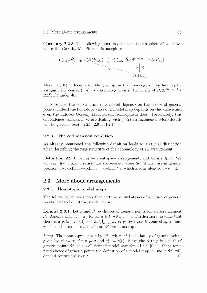
Corollary 2.2.3. The following diagram defines an isomorphism Ψx which wewill call a Goresky-MacPherson isomorphism.

⊕u∈P H∗−dim(u)(∆(P<u))

Ψx

Σ∼=

⊕u∈P H∗(Sdim(u)−1 ∗ ∆(P<u))

Φx∗∼=

H∗(LA)

Moreover, Φx∗ induces a double grading on the homology of the link LA by

assigning the degree (r, u) to a homology class in the image of Hr(Sdim(u)−1 ∗∆(P<u)) under Φx

∗ .

Note that the construction of a model depends on the choice of genericpoints. Indeed the homotopy class of a model map depends on this choice andeven the induced Goresky-MacPherson isomorphism does. Fortunately, thisdependence vanishes if we are dealing with (≥ 2)-arrangements. More detailswill be given in Section 2.3, 2.9 and 2.10.

2.2.3 The codimension condition

As already mentioned the following definition leads to a crucial distinctionwhen describing the ring structure of the cohomology of an arrangement.

Definition 2.2.4. Let A be a subspace arrangement, and let u, v ∈ P . Wewill say that u and v satisfy the codimension condition if they are in generalposition, i.e., codimu+codim v = codim u∩v, which is equivalent to u+v = Rn.

2.3 More about arrangements

2.3.1 Homotopic model maps

The following lemma shows that certain perturbations of a choice of genericpoints lead to homotopic model maps.

Lemma 2.3.1. Let x and x′ be choices of generic points for an arrangementA. Assume that xu = x′

u for all u ∈ P with u 6= v. Furthermore, assume thatthere is a path p : [0, 1] −→ Sv \

⋃u>v Su of generic points connecting xv and

x′v. Then the model maps Φx and Φx′

are homotopic.

Proof. The homotopy is given by Φxt, where xt is the family of generic points

given by xtu := xu for u 6= v and xt

v := p(t). Since the path p is a path ofgeneric points Φxt

is a well defined model map for all t ∈ [0, 1]. Since for afixed choice of generic points the definition of a model map is unique Φxt

willdepend continuously on t.


2.3.2 Products with euclidean space

The following easy fact, together with Proposition 2.6.23 will allow us to

restrict ourselves to classes in Ψx(H∗(∆(P<u)

)and Ψx

(H∗(∆(P<v))

)with

u ∩ v = 0 when calculating products.

Proposition 2.3.2. Let A be an arrangement in Rn, identify Rm+n withRm×Rn and accordingly Sm+n−1 with Sm−1 ∗Sn−1. For u ∈ A set u′ := Rm×uand let A′ := {u′ : u ∈ A} be the arrangement in Rm+n corresponding to Aand having link LA′ = Sm−1 ∗ LA. Orient Su′ by [Sm−1] ∗ [Su].

Assume that generic points {xu} for A and {x′u′} for A′ are chosen in such

a way that x′u′ ∈ Sm−1 ∗ {xu} for all u ∈ A. Let h : Sm−1 ∗ LA → LA′ be

the homotopy equivalence defined by identifying ∆(P<u) with ∆(P ′<u′) and

Sm−1 ∗ Sdim(u)−1 with Sdim(u′)−1. Then Φ′◦h ' idSm−1 ∗ Φ.

Proof. Move the points.

2.4 A product for order complexes

We will now describe a product on the homology of certain order complexesthat will be used to describe the ring structure on the homology of the link ofan arrangement.

Throughout this section, let P and Q be lattices. We will denote all topelements by > and all bottom elements by ⊥. As usual the least upper boundof elements a and b will be denoted by a∨ b and their greatest lower bound bya ∧ b.

Note that ∆(P ×Q) is just ∆(P )×∆(Q) endowed with the usual simplicialstructure that a product of two simplicial complexes is given. Therefore, thereis the well known map

C∗(P ) ⊗ C∗(Q)×−→ C∗(P × Q),

and on the right side of the arrow no harmful confusion is possible. It is givenby

〈u0, . . . , ur〉 ⊗ 〈v0, . . . , vs〉 7→∑

0=i0≤···≤ir+s=r0=j0≤···≤jr+s=s

(ik−1,jk−1) 6=(ik,jk) ∀k

σi,j〈(ui0 , vj0), . . . , (uir+s , vjr+s)〉

for chains u0 < u1 < · · · < ur and v0 < v1 < · · · < vs, where the σi,j are signsdetermined by σi,j = 1 if k = 0 or l = 0 and by d(a× b) = da× b+(−1)ra×db.

Although ∆(P ) itself is contractible, this product induces useful productsin homology, the most import one for our purposes being

Hk+2(P, P<> ∪ P>⊥) ⊗ Hl+2(Q,Q<> ∪ Q>⊥)

→ Hk+l+2+2(P × Q, (P × Q)<> ∪ (P × Q)>⊥).

2.5 A ring defined by the combinatorial data 37

The reader be warned that we have written P<> ∪P>⊥ for ∆(P<>)∪∆(P>⊥),although really we should not have done so. The above dimensions have been

chosen because of Hk

(P<>

>⊥

)∼= Hk+2(P, P<>∪P>⊥), since ∆(P ) is a cone over

a cone over ∆(P<> ∪ P>⊥). Let us fix an isomorphism

C>⊥ : Hk

(P<>

>⊥

)→ Hk+2(P, P<> ∪ P>⊥)

which is given on the chain level by

〈u0, . . . , uk〉 7→ (−1)k+2〈⊥, u0, . . . , uk,>〉.

The sign is chosen to make it possible to think of this map as a 7→ 〈>,⊥〉 ∗ a.C>⊥ can be decomposed into two isomorphisms

Hk

(P<>

>⊥

)C⊥−−→ Hk+1

(P<>, P<>

>⊥

)C>−−→ Hk+2(P, P<> ∪ P>⊥)

or

Hk

(P<>

>⊥

)C>−−→ Hk+1

(P>⊥, P<>

>⊥

)−C⊥−−−→ Hk+2(P, P<> ∪ P>⊥)

where

C⊥(〈u0, . . . , uk〉) := 〈⊥, u0, . . . , uk〉,C>(〈u0, . . . , uk〉) := (−1)k+1〈u0, . . . , uk,>〉.

Note that in both of the compositions the first arrow is just the inverse of d.This leads to the following

Definition 2.4.1. For lattices P , Q we define

λ : Hk

(P<>

>⊥

)⊗ Hl

(Q<>

>⊥

)→ Hk+l+2

((P × Q)<>

>⊥

)by

a ⊗ b 7→ C−1>⊥(C>⊥(a) × C>⊥(b)).

2.5 A ring defined by the combinatorial data

In this section we define the ring that under favourable circumstances will beisomorphic to the homology of the link of an arrangement endowed with thelinking product.


Remember, that if P is the intersection poset of an arrangement A in Rn,it always contains a top element, and that by P we denote P ∪ {Rn}, which isa lattice with ⊥ = Rn.

Now if u, v ∈ P<0 span the whole of Rn, the map ∨ : P≤u × P≤v → P≤u∨v isa monomorphism (and even an isomorphism, if all elements of A contain u orv) and induces a map

∨∗ : H∗

((P≤u × P≤v)<(u,v)

>⊥

)→ H∗(P<u∨v).

This allows for the following

Definition 2.5.1. Let P be the intersection lattice of an arrangement and letε, dim be the additional combinatorial data.

We will define a ring structure on R =⊕

u∈P H∗(∆(P<u)) via the product

◦ : Hr(∆(P<u)) ⊗ Hs(∆(P<v)) → Hr+s+2(∆(P<u∨v)),

which we call the combinatorial linking product, by

a ◦ b :=

εu,v(−1)n+r(n−dim v) ∨∗ (λ(a ⊗ b)),

if dim(u ∨ v) = dim u + dim v − n,

0, otherwise.

Here, of course, n = dim⊥.

Note that in the case of an arrangement with all dimensions even, fordim(u ∨ v) = dim u + dim v − n this reduces to a ◦ b = εu,v ∨∗ (λ(a ⊗ b)) andfor a complex arrangement even to a ◦ b = ∨∗(λ(a ⊗ b)). This is exactly theproduct defined in [Yuz98].

Remark 2.5.2. Defining a ∗ b for suitable chains and homology classes by

C⊥(a ∗ b) = ∨∗(C⊥a × C⊥b)

we have

−C⊥Cu∨v(∨∗λ(a ⊗ b)) = ∨∗(Cu⊥a × Cv⊥b) = C⊥(Cua ∗ Cvb),

which yields

∨∗ λ(a × b) = d(Cu∨v ∨∗ λ(a ⊗ b)) = −d(Cua ∗ Cvb) =

= −d(u ∗ a ∗ v ∗ b) = (−1)|a|d(u ∗ v ∗ a ∗ b)

and therefore

a ◦ b =

εu,v(−1)n+r(n−dim v+1)(−〈u〉 + 〈v〉) ∗ a ∗ b,

if dim(u ∨ v) = dim u + dim v − n,

0, otherwise.

This relates our definition to the formulae obtained in Chapter 1 (respectivelyin [Lon00]) and to the Introduction 2.1.

2.6 Topological preliminaries 39

2.6 Topological preliminaries

In this section we gather some topological facts, for the largest part fromhomology theory, that we will use. Since we are interested in links of arrange-ments and the unit sphere in a product of euclidean spaces is a join of theunit spheres in the spaces involved, we have to deal with joins if we considerproducts of arrangements. We treat joins first.

Our approach to the cohomolgy of the complement of an arrangement isvia the homology of the link. Since these are isomorphic via Alexander dualityand we are interested in the cup product in cohomology, we have to considerthe corresponding product on homology, which we call the linking product.The largest part of this section is devoted to the study of the linking product,which we prepare by taking a short look at the related intersection product.

The material in this section is fairly standard, but sign and orientationconventions of different authors do not always agree, so we have tried to beexplicit about them. Those here should coincide with those in [Dol72].

All spaces, pairs, etc. will be expected to fulfill niceness properties notstated explicitly. Finite simplicial complexes will always suffice.

2.6.1 Joins of spaces and of homology classes

Definition 2.6.1. The join X ∗ Y of two non-empty spaces X and Y is thequotient of the product X × I × Y by the equivalence relation generated by(x, 0, y) ∼ (x, 0, y′) and (x, 1, y) ∼ (x′, 1, y) for all x, x′ ∈ X, y, y′ ∈ Y . We alsodefine X ∗ ∅ := X, ∅ ∗ Y := Y . For pairs of spaces we set (X,A) ∗ (Y,B) :=(X ∗ Y,A ∗ Y ∪ X ∗ B).

Note 2.6.2. Care is needed, because in general (X, ∅) ∗ (Y, ∅) 6= (X ∗ Y, ∅).Let p denote the quotient map (X,A)× (I, dI)× (Y,B) → (X,A) ∗ (Y,B).

Proposition 2.6.3. The induced map

p∗ : H∗((X,A) × (I, dI) × (Y,B)) → H∗((X,A) ∗ (Y,B))

is an isomorphism. For p ∈ X, q ∈ Y the map

H∗(X ∗ Y ) → H∗((X, {p}) ∗ (Y, {q}))is an isomorphism.

Definition 2.6.4. For a ∈ Hr(X,A), b ∈ Hr(Y,B), we define a ∗ b ∈Hr+s+1((X,A) ∗ (Y,B)) by a ∗ b := p∗(a × [I] × b), where [I] is the genera-tor of H1(I, dI) defined by d[I] = −〈0〉 + 〈1〉.Remark 2.6.5. This definition is consistent with defining the join of twosimplices by juxtaposition of vertices.


Definition 2.6.6. We define a join product for reduced homology by commu-tativity of

H∗(X) ⊗ H∗(Y )∼=

∗

H∗(X, {p}) ⊗ H∗(Y, {q})∗

H∗(X ∗ Y )∼= H∗

((X, {p}) ∗ (Y, {q})),

if X 6= ∅, Y 6= ∅, and by requiring that the join with the positive generator ofH−1(∅) be the identity otherwise. Similarly we define a join product for thereduced homology of a space and the homology of a pair.

Proposition 2.6.7. The above product does not depend on the choice ofpoints p and q and is therefore well-defined.

Some of the following propositions will be formulated for pairs only, evenif we also need the corresponding statements about reduced homology.

Proposition 2.6.8. Let t : X ∗Y → Y ∗X be the homeomorphism [x, λ, y] 7→[y, 1− λ, x] and A ⊂ X, B ⊂ Y , a ∈ H∗(X,A), b ∈ H∗(Y,A). Then t∗(a ∗ b) =(−1)(|b|+1)(|a|+1)b ∗ a.

Proof. The corresponding statement for the homology cross product is [Dol72,Chap. VII, Eq. 2.8].

Proposition 2.6.9. Consider the homeomorphisms

h1 : d(Dk × Dl) → Sk+l−1

x 7→ x

‖x‖

and

h2 : Sk−1 ∗ Sl−1 → Sk+l−1

[x, λ, y] 7→ ((1 − λ)x, λy)

‖((1 − λ)x, λy)‖ .

The diagram

Hk(Dk, Sk−1) ⊗ Hl(D

l, Sl−1)d⊗d

×

Hk−1(Sk−1) ⊗ Hl−1(S

l−1)

∗

Hk+l(Dk × Dl, d(Dk × Dl))

d

Hk+l−1(Sk−1 ∗ Sl−1)

h2∗

Hk+l−1(d(Dk × Dl))h1∗

Hk+l−1(Sk+l−1)

commutes, and therefore, given orientations on Dk and Dl, the two orientationsof Sk+l−1 indicated by the diagram coincide.


Proposition 2.6.10. Let P = {p} be a space containing exactly one point.For a pair (X,A) define C(X,A) := (P, ∅)∗ (X,A) = (P ∗X,X ∪P ∗A). Thenfor compact pairs (Xi, Ai), i ∈ {1, 2} the diagram

H∗(X1, A1) ⊗ H∗(X2, A2)

∗

∼=(〈p〉∗)⊗(〈p〉∗)

H∗(C(X1, A1)) ⊗ H∗(C(X2, A2))

×

H∗(C(X1, A1) × C(X2, A2))

f∗∼=

H∗((X1, A1) ∗ (X2, A2)) ∼=〈p〉∗

H∗(C((X1, A1) ∗ (X2, A2))),

where

f : C(X1, A1) × C(X2, A2) → C((X1, A1) ∗ (X2, A2))([p, λ1, x1], [p, λ2, x2]

) 7→{[

0, λ2, [x1,λ1

2λ2, x2]

], λ2 ≥ λ1,[

0, λ1, [x2, 1 − λ2

2λ1, x1]

], λ1 ≥ λ2,

commutes.

2.6.2 The intersection product

Let Mm be a compact oriented manifold, [M ] ∈ Hm(M) the orientation class.

Definition 2.6.11. For A ⊂ X ⊂ M we denote by D the Poincare-Alexander-Lefschetz duality isomorphism

D : Hr(X,A) → Hm−r(M − A,M − X)

given byD(a) ∩ [M ] = a.

Definition 2.6.12. For A ⊂ X ⊂ M and B ⊂ Y ⊂ M we define the intersec-tion product

• : Hr(X,A) ⊗ Hs(Y,B) → Hr+s−m(X ∩ Y, (A ∪ B) ∩ (X ∩ Y ))

by requiring thatD(a • b) = D(a) ∪ D(b).

Proposition 2.6.13. We have

(i) a • b = (−1)(m−|a|)(m−|b|)b • a,

(ii) [M ] • a = a • [M ] = a.


Proof. Compare [Dol72, VII.8.7,VII.8.9,VIII.13.8,VIII.13.10].

Proposition 2.6.14. Let Nn be another compact oriented manifold, and letM × N be oriented by

[M × N ] = ε([M ] × [N ]),

ε ∈ {−1, +1}. For a, c and b, d homology classes of appropriate subspaces ofM respectively N (or pairs) we have

(a × b) • (c × d) = ε · (−1)(n−|b|)(m−|c|)(a • c) × (b • d).

Proof. Compare [Dol72, VII.8.16,VIII.13.13]

Using Proposition 2.6.3 we have as an immediate consequence the following

Proposition 2.6.15. Let Ai ⊂ Xi ⊂ Sk, Bi ⊂ Yi ⊂ Sl, Ai, Bi 6= ∅, ai ∈H∗(Xi, Ai), bi ∈ H∗(Yi, Bi) for i ∈ {0, 1}. Then

(a0 ∗ b0) • (a1 ∗ b1) = ε · (−1)(l−|b0|)(k−|a1|)(a0 • a1) ∗ (b0 • b1),

if [Sk ∗ Sl] = ε([Sk] ∗ [Sl])

2.6.3 The linking product

The exact definition of Alexander duality in dimensions 0 and n − 1 varies.The following form seems to be best suited to our application.

Definition 2.6.16. Let X ⊂ Sn−1, q ∈ Sn−1\X. By ADq we denote theAlexander duality isomorphism

ADq : Hr(X) → Hn−2−r(Sn−1\X, {q})given by

ADq(da) = D(a)

ie the inverse of the composite

Hn−2−r(Sn−1\X, {q}) ∩[Sn−1]

∼= Hr+1(Sn−1\{q}, X)d∼= Hr(X).

We will often simply write AD instead of ADq.

Definition 2.6.17. For X,Y ⊂ Sn−1, q ∈ Sn−1\(X ∪ Y ) we define the linkingproduct

◦ : Hr(X) ⊗ Hs(Y ) → Hr+s+2−n(X ∪ Y )

byADq(a ◦ b) = ADq(a) ∪ ADq(b).


Note 2.6.18. If either r or s equals n− 2, the linking product depends on thepoint q. However, it only depends on the connected component of Sn−1\(X∪Y )in which q lies.

Remark 2.6.19. For the special case r + s = n − 2, X, Y disjoint connectedoriented manifolds of dimensions r and s, this yields just the familiar linkingnumber.

Proposition 2.6.20. We have a ◦ b = d((d−1a) • (d−1b)).

Proof. AD(a ◦ b) = AD(a) ∪ AD(b) = D(d−1a) ∪ D(d−1b) = D((d−1a) •(d−1b)) = AD(d((d−1a) • (d−1b))).

The next proposition states that unlinked subspaces have trivial linkingproduct. We will use it in Section 2.8.

Proposition 2.6.21. Let Xi ⊂ Sn−1 for i = 0, 1. If there exist Bi ⊃ Xi

such that the maps Hri(Xi) → Hri

(Bi) induced by inclusion are trivial andB0 ∩B1 = ∅ and q /∈ B0 ∪B1, then the linking product Hr0(X0)⊗ Hr1(X1) →Hr0+r1+2−n(X0 ∪ X1) is trivial.

Proof. The linking product in question is the composition of the second columnof the following commutative diagram.

Hr0+1(B0, X0) ⊗ Hr1+1(B1, X1)d⊗d

•

Hr0(X0) ⊗ Hr1(X1)

Hr0+r1+3−n(∅) Hr0+1(Sn−1\{q}, X0) ⊗ Hr1+1(Sn−1\{q}, X1)

d⊗d ∼=

•

Hr0+r1+3−n(Sn−1\{q}, X0 ∪ X1)

d

Hr0+r1+2−n(X0 ∪ X1)

The surjectivity of the map in the first row follows from the long exact se-quences of the pairs (Bi, Xi), and of course H∗(∅) ∼= 0.

Corollary 2.6.22. If Xi ⊂ Sn−1, i = 1, 2, lie on different sides of an (n − 2)-sphere embedded in Sn−1, then the linking product Hr1(X1) ⊗ Hr2(X2) →Hr1+r2+2−n(X1 ∪ X2) is trivial for ri < n − 2.

Proof. Choose the Bi to be the components of the complement of the (n− 2)-Sphere in Sn−1\{q}. Each of them is homotopy equivalent to either a point orSn−2 and therefore Hri

(Bi) ∼= 0.


2.6.4 Linking products in joins of spheres

The following constructions are dual to the exterior cohomology product.

Proposition 2.6.23. Let X ⊂ Sn−1. Consider Sm−1 ∗ X ⊂ Sm−1 ∗ Sn−1,orient Sm+n−1 = Sm−1 ∗ Sn−1 by [Sm−1] ∗ [Sn−1], and use q ∈ Sn−1\X to defineAlexander Duality in Sn−1 as well as Sm+n−1. Then the map

j : H∗(X) → H∗(Sm−1 ∗ X)

a 7→ (−1)m[Sm−1] ∗ a

is an isomorphism shifting degree by m and respecting linking products.

Proof. That j is an isomorphism shifting degrees, if not clear anyway, followsfrom Proposition 2.6.3 and the Kunneth theorem. Additionally we have

j(a ◦ b) = (−1)m[Sm−1] ∗ d(d−1a • d−1b)

= d([Sm−1] ∗ (d−1a • d−1b))

= d(([Sm−1] ∗ d−1a) • ([Sm−1] ∗ d−1b))

= d(d−1([Sm−1] ∗ a) • d−1([Sm−1] ∗ b))

= j(a) ◦ j(b)

using Proposition 2.6.13 and Proposition 2.6.15.

Remark 2.6.24. This isomorphism is dual to the isomorphism of the coho-mology rings of the complements induced by inclusion.

Proposition 2.6.25. Let X ⊂ Sm−1, Y ⊂ Sn−1. Let qX ∈ Sm−1\X, qY ∈Sn−1\Y and define Alexander duality in (Sm−1, X) ∗ (Sn−1, Y ) = (Sm+n−1, X ∗Sn−1 ∪ Sm−1 ∗ Y ) via a q ∈ {qX} ∗ {qY }. Orient Sm+n−1 = Sm−1 ∗ Sn−1 byε([Sm−1] ∗ [Sn−1]), ε ∈ {+1,−1}. Then the diagram

H∗(X) ⊗ H∗(Y )(∗[Sn−1])⊗([Sm−1]∗)

H∗(X ∗ Sn−1) ⊗ H∗(Sm−1 ∗ Y )

◦H∗(Sm−1\{qX}, X) ⊗ H∗(Sn−1\{qY }, Y )

ε·∗

∼= (−1)md⊗d

H∗((Sm−1\{qX}, X) ∗ (Sn−1\{qY }, Y ))d

H∗(X ∗ Sn−1 ∪ Sm−1 ∗ Y )

commutes.

Proof. Let a ∈ H∗(Sm−1\{qX}, X), b ∈ H∗(Sn−1\{qY }, Y ). Then

ε · d(a ∗ b) = d((a ∗ [Sn−1]) • ([Sm−1] ∗ b))

= d(a ∗ [Sn−1]) ◦ d([Sm−1] ∗ b)

= (−1)m(da ∗ [Sn−1]) ◦ ([Sm−1] ∗ db)

by Proposition 2.6.15 and Proposition 2.6.20.

2.7 Products of classes satisfying the codimension condition 45

2.7 Products of classes satisfying the codimension con-dition

We now turn to our main objective: For an arrangement A with intersectionposet P , compare the combinatorial linking product on R =

⊕u∈P H

(∆(P<u)

)with the linking product on H∗(LA) via the isomorphisms of Z-graded abeliangroups Ψx : R → H∗(LA).

This section deals with products Ψx(a) ◦ Ψx(b) for classes a ∈ H(∆(P<u)

)and b ∈ H

(∆(P<v)

)belonging to pairs u, v that satisfy the codimension con-

dition.

2.7.1 Strategy

We will give a brief description of the idea behind the material in this section.If u + v = Rn and we consider the (n− dim v)-dimensional arrangement Au ={w/(u∩v) : w ⊃ u} and the (n−dim u)-dimensional arrangement Av = {z/(u∩v) : z ⊃ v}, we will be able to find an inclusion

(u ∩ v) ×(v/(u ∩ v),

⋃Av

)×

(u/(u ∩ v),

⋃Au

)→

(Rn,

⋃A

)respectively

Su∩v ∗(Sv/(u∩v), LAv

) ∗ (Su/(u∩v), LAu

) → (Sn−1, LA

).

Therefore we essentially deal with an exterior product, the description of whichshould be feasible.

2.7.2 The signs εu,v

Let us first get two working descriptions of our signs εu,v for an arrangementin Rn with intersection poset P .

Proposition 2.7.1. Let u, v ∈ P , u + v = Rn. Let z be a subspace of Rn

complementary to u∩v. Let u′ = u∩z and v′ = v∩z. Identify u with (u∩v)×u′,v with (u ∩ v) × v′, Rn with (u ∩ v) × v′ × u′, and the corresponding spheresaccordingly. Now if u′ and v′ and the corresponding spheres are orientedsuch that under the described identifications [Su] = [Su∩v] ∗ [Su′ ] and [Sv] =[Su∩v] ∗ [Sv′ ], then [Sn−1] = εu,v[Su,v] ∗ [Sv′ ] ∗ [Su′ ].

Proof. The analogous statement about orientations of disks and their productswould be just the definition of ε in Section 2.2, and the two are connected byProposition 2.6.9.

Proposition 2.7.2. Let u, v ∈ P , u + v = Rn. Then [Su] • [Sv] = εu,v[Su∩v].Here [S0] is assumed to be the positive generator of H−1(∅).


Proof. Let the notation be that of the preceding proposition and denote thepositive generator of H−1(∅) by ∅. Then

[Su] • [Sv] = εu,v

([Su∩v] ∗ ∅ ∗ [Su′ ]

) • ([Su∩v] ∗ [Sv′ ] ∗ ∅) =

= εu,v

([Su∩v] • [Su∩v]

) ∗ (∅ • [Sv′ ]) ∗ (

[Su′ ] • ∅) =

= εu,v[Su∩v] ∗ ∅ ∗ ∅ = εu,v[Su∩v]

by Proposition 2.6.15 and Proposition 2.6.13.

2.7.3 Geometrical description of the linking product in a link

Let A be an arrangement in Rn, u, v ∈ P and u + v = Rn, u ∩ v = 0. In thiscase we can identify Sn−1 with Sv ∗ Su. Let Lv

u := Sv ∩⋃{w ∈ A : w < u}.

Note that Lvu ∗ Su ⊂ LA. Define

φvu : ∆(P<u) → Lv

u

like φu earlier, but withφv

u(w) = xv∩w.

Now choose generic points x′w, such that xw ∈ x′

w∩v ∗ Su for all w < u andSv∗xw ∈ x′

w∩u for all w < v. Comparing the subarrangement of A consisting ofall subspaces containing v and the arrangement in u given by the intersectionswith u of the former subspaces, we are just in the situation of Proposition 2.3.2.Therefore, for b ∈ H∗(∆(P<v)) we have

Ψx(b) = Φx∗([Sdim(v)−1] ∗ b) = [Sv] ∗ (φ′u

v)∗(b)

and for a ∈ H∗(∆(P<u))

Ψx(a) = Φx∗([Sdim(u)−1] ∗ a) = (−1)(dim u)(|a|+1)(φ′v

u)∗(a) ∗ [Su],

where the sign comes from Proposition 2.6.8.Now, using Proposition 2.6.25 we get((−1)(dim u)(|a|+1)(φ′v

u)∗(a) ∗ [Su]) ◦ (

[Sv] ∗ (φ′uv)∗(b)

)=

= εu,v · (−1)dim v+(dim u)(|a|+1)d(d−1(φ′vu)∗(a) ∗ d−1(φ′u

v)∗(b)),

since the ε in Proposition 2.6.25 has been identified as εu,v in Proposition 2.7.1.We summarize:

Proposition 2.7.3. Let A be an arrangement in Rn, u, v ∈ P and u + v =Rn, u ∩ v = 0. There is a choice of generic points {xw} such that for alla ∈ H∗(∆(P<u)) and b ∈ H∗(∆(P<v)) we have

Ψx(a) ◦ Ψx(b) = εu,v · (−1)dim v+(dim u)(|a|+1)d(d−1(φvu)∗(a) ∗ d−1(φu

v)∗(b)).

Here, Sn−1 is identified with Sv∗Su. Given an arbitrary choice of generic points{x′

w}, x can be chosen in such a way that Ψx and Ψx′agree on H∗(∆(P<u))

and H∗(∆(P<v)).

2.7 Products of classes satisfying the codimension condition 47

When compared with the expression in Remark 2.5.2 this already lookspromising.

2.7.4 Combinatorial description of the linking product.

Now that we have a nice geometrical description of the product of two classessatisfying the codimension condition, we are ready to describe it in terms ofthe combinatorial data. The rest of this section will be devoted to proving thefollowing

Proposition 2.7.4. Let A be an arrangement in Rn, u, v ∈ P and u+v = Rn.There is a choice of generic points {xw} such that for all a ∈ H∗(∆(P<u)) andb ∈ H∗(∆(P<v)) we have

Ψx(a) ◦ Ψx(b) = Ψx(a ◦ b),

where the product on the right hand side refers to the combinatorial one givenin Definition 2.5.1. For an arbitrary choice of generic points {x′

w}, x can be cho-sen in such a way that Ψx and Ψx′

agree on H∗(∆(P<u)) and b ∈ H∗(∆(P<v)).

Caution 2.7.5. The generic points {xw} above depend on u and v.

Lemma 2.7.6. If Proposition 2.7.4 is true for all arrangements A and all u, vwith u ∩ v = 0, then it is true in general.

Proof. Because of the naturality of the linking product with respect to inclu-sions, we can calculate it in the subarrangement of A consisting of all subspacescontaining u ∩ v. This in turn gives rise to an arrangement A′ by consideringthe intersections with a subspace of Rn complementary to u ∩ v, which is re-lated to A in the manner described in Proposition 2.3.2 (with the roles of Aand A′ exchanged). Combining this with Proposition 2.6.23 we get

Ψx(a ◦ b) = [Su∩v] ∗ Ψx′(a′ ◦ b′),

where a, b can be identified with a′, b′ and the primes are only needed to dis-tinguish the combinatorial ◦ in the different rings, and

Ψx(a) ◦ Ψx(b) =([Su∩v] ∗ Ψx′

(a′))◦

([Su∩v] ∗ Ψx′

(b′))

=

= (−1)dim(u∩v)[Su∩v] ∗(Ψx′

(a′) ◦ Ψx′(b′)

).

Thus the sign in the definition of a ◦ b should be (−1)dim(u∩v) times the signin a′ ◦ b′, which is the case if n = n′ + dim(u ∩ v), n − dim v = n′ − dim v′,εu,v = ε′u′,v′ . Only the latter needs to be checked, and we have

εu,v[Su∩v] = [Su] • [Sv] = ([Su∩v] ∗ [Su′ ]) • ([Su∩v] ∗ [Sv′ ]) =

= ([Su∩v] • [Su∩v]) ∗ ([Su′ ] • [Sv′ ]) = ε′u′,v′ [Su∩v],

using Proposition 2.7.2.


Proposition 2.7.7. In the situation of Proposition 2.7.3 and with the termi-nology of Section 2.5 we have

d(d−1φv

u(a) ∗ d−1φuv(b)

)= ∨∗(λ(a ⊗ b)).

Proof. Denote the point of Sn−1\LA used to define Alexander duality by q.Assume that points qu ∈ Su\Lu

v , qv ∈ Sv\Lvu are chosen such that q is halfway

between qv and qu. q will have to be moved to achieve this, but this does notmatter, since Alexander duality depends only on the connected component ofSn−1\LA in which q lies. Set xu = −qu, xv = −qv. Additionally to the xw

chosen for u ∈ P<0, set x0 = 0, x⊥ = −q and extend φ0, φvu, φu

v accordingly(1-simplices involving x0 will of course be mapped to straight lines, all othersstill to geodesics). In Proposition 2.7.3 we have already chosen x such thatxw∨z ∈ {xw∨v} ∗ {xu∨z} for all w ∈ P<u and z ∈ P<v. Assume that they areindeed at the center of that line and note that this now holds for all w ∈ P≤u

and z ∈ P≤v. Now consider the diagram in Figure 2.1 on page 49. The diagramis commutative: α is essentially Proposition 2.6.10, β commutes because of ourchoice of φv

u(⊥) = xv = −qv, φuv(⊥) = xu = −qu. γ commutes because of our

choice of xw∩z above. Commutativity of δ and ε is due to φvu(u) = φu

v(v) = x0.Now the composition of the arrow on top with the arrows on the extreme rightis the left hand side of the equation to be proved, while the arrows on the lefttogether with the bottom arrow yield the right hand side.

Proof of Proposition 2.7.4. Because of Lemma 2.7.6 we may assume u∩v = 0,thus we just have to show that combining Proposition 2.7.3 with Proposi-tion 2.7.7 yields the correct sign, and indeed

(−1)dim v+(dim u)(|a|+1) = (−1)n+|a|(n−dim v),

since dim u + dim v = n.

2.8 Products of classes not satisfying the codimensioncondition

Assuming that the arrangement A does not contain real hyperplanes we showthat for any pair u, v ∈ P that does not satisfy the codimension conditionthere is pair of model maps leading to trivial multiplication.

Proposition 2.8.1. Let A be a subspace arrangement in Rn not containingreal hyperplanes with intersection poset P . Let u, v ∈ P be two subspacesthat do not satisfy the codimension condition, i.e., u + v 6= Rn. Then there isa pair of model maps Φx, Φx′

: LA −→ LA such that the following composition

2.8 Products of classes not satisfying the codimension condition 49

Hr(P<u)⊗Hs(P<v)(φv

u)∗⊗(φuv )∗

C⊥⊗C⊥

Cu⊥⊗Cv⊥

Hr(Lvu)⊗Hs(Lu

v )

d−1⊗d−1

βHr+1(P<u,P<u)⊗Hs+1(P<v,P<v)

(φvu)∗⊗(φu

v )∗

Cu⊗Cv Hr+1(Sv\{qv},Lvu)⊗Hs+1(Su\{qu},Lu

v )

(x0∗)⊗(x0∗)

∗

δ

Hr+2(P≤u,P<u∪P≤u)⊗Hs+2(P≤v,P<v∪P≤v)

×

(φvu)∗⊗(φu

v )∗

Hr+2(Dv,Sv∪0∗Lvu)⊗Hs+2(Du,Su∪0∗Lu

v )

× αHr+s+4(P≤u×P≤v,(P≤u×P≤v)<(u,v)∪(P≤u×P≤v)>⊥)

C−1(u,v)

(φvu×φu

v )∗C−1

(u,v)⊥Hr+s+4(Dv×Du,Dv×Su∪Sv×Du∪0∗(Dv×Lu

v∪Lvu×Du))

(x0∗)−1

ε

Hr+s+3

((P≤u×P≤v)<(u,v),(P≤u×P≤v)<(u,v)

>⊥

)

(φvu×φu

v )∗

∨∗

C−1⊥

Hr+s+2

((P≤u×P≤v)<(u,v)

>⊥

)

∨∗

Hr+s+3(Dv×Su∪Sv×Du,Dv×Luv∪Lv

u×Du)

γ

Hr+s+3(P<0,P<0)(φ0)∗

d

Hr+s+3(Sv∗Su,Sv∗Luv∪Lv

u∗Su)

d

Hr+s+2(P<0)(φ0)∗

Hr+s+2(Sv∗Luv∪Lv

u∗Su)

Hr+s+2(P<0)Ψx′

Hr+s+2(LA)

Figure 2.1: Diagram needed in the proof of Proposition 2.7.7.


is the zero map.

Hr(Sdim u−1 ∗ ∆(P<u)) ⊗ Hs(Sdim v−1 ∗ ∆(P<v))Φx∗⊗Φx′∗−−−−→ Hr(LA) ⊗ Hs(LA)

(2.1)◦−−−−→ Hr+s+2−n(LA).

Before proving Proposition 2.8.1 we will spend some time on thickening thearrangement, i.e., replacing all subspaces by a thickened copy, to have spacefor further constructions.

Definition 2.8.2. Let A be a subspace arrangement in Rn, ~n ∈ Rn a unitvector. For ξ ∈ R we define the slanted arrangement in direction ~n

A(~n, ξ) = {a + ξ · ~n : a ∈ A},and for ε > 0 we define the thickened arrangement in direction ~n using thesame notation

A(~n, [−ε, +ε]) = {a + [−ε, +ε] · ~n : a ∈ A}.Proposition 2.8.3. For sufficiently small ε > 0 the following inclusions arehomotopy equivalences for every ξ ∈ [−ε, +ε]:

Sn−1 ∩⋃

a∈A(~n,ξ)

a ↪−→ Sn−1 ∩⋃

a∈A(~n,[−ε,+ε])

a ,

Sn−1 \⋃

a∈A(~n,[−ε,+ε])

a ↪−→ Sn−1 \⋃

a∈A(~n,ξ)

a .

Now consider the following orientation preserving homeomorphism γξ : Sn−1 →Sn−1 of the pairs (Sn−1, LA) and (Sn−1, Sn−1 ∩⋃

a∈A(~n,ξ) a) which is just travel-ling along a geodesic from −~n to ~n the right amount of time. In formulae:

x ∈ LAγξ7−→ t · x + ξ · ~n,

where t ≥ 0 is such that ‖t · x + ξ · ~n‖ = 1. Then the following composition ofmaps yields a homotopy equivalence for every ξ ∈ [−ε, +ε] and any two suchare homotopic:

LAγξ−→ Sn−1 ∩

⋃a∈A(~n,ξ)

a ↪−→ Sn−1 ∩⋃

a∈A(~n,[−ε,+ε])

a.

Using the same construction we also obtain a homotopy equivalence

MA'−→ Sn−1 \

⋃a∈A(~n,ξ)

a.

2.8 Products of classes not satisfying the codimension condition 51

The homotopy equivalences are such that the following diagram commutes

H∗(LA)

ADq

∼=H∗(Sn−1∩⋃

a∈A(~n,ξ) a)

ADq′

∼=H∗(Sn−1∩⋃

a∈A(~n,[−ε,+ε]) a)

ADq′

H∗(MA,{q}) H∗(Sn−1\⋃a∈A(~n,ξ) a,{q′})∼= ∼=H∗(Sn−1\⋃a∈A(~n,[−ε,+ε]) a,{q′}),

where q′ = γξ(q).

Proof of Proposition 2.8.1. The construction of the maps Φx and Φx′splits up

into two parts. One is concerned with the order complex maps φu, u ∈ P ,whereas the other one is concerned with the sphere portion.

The order complex portion

If the codimension condition is not satisfied there certainly is a hyperplaneH ⊂ Rn containing u + v. Let ~n be a unit normal vector to H. Construct twomodel maps Φx and Φx′

by choosing the generic points in such a way that theimages of ∆(P<u) under Φx, respectively ∆(P<v) under Φx′

, are situated ondifferent sides of H, say

〈~n, Φx(∆(P<u))〉 ≥ 0 ,

〈~n, Φx′(∆(P<v))〉 ≤ 0 .

The sphere portion

If two spaces u, v ∈ P have non–empty intersection there is no model mapgiven by ιu ∗ φu, u ∈ P , such that the images of ιu : Sdim(u)−1 → LA andιv : Sdim(v)−1 → LA are disjoint. Therefore we thicken the arrangement. ByProposition 2.8.3 we can compute the linking product in the space Sn−1 ∩⋃

a∈A(~n,[−ε,+ε]) a for a suitable choice of ε > 0. We consider the compositions

LAΦx−→ LA

γ+ε−−→ Sn−1 ∩⋃

a∈A(~n,+ε)

a ↪−→ Sn−1 ∩⋃

a∈A(~n,[−ε,+ε])

a , respectively

LAΦx′−→ LA

γ−ε−−→ Sn−1 ∩⋃

a∈A(~n,−ε)

a ↪−→ Sn−1 ∩⋃

a∈A(~n,[−ε,+ε])

a.

Consider the images of Sdim(u)−1 ∗ ∆(P<u) under the first map, respectively ofSdim(v)−1 ∗ ∆(P<v) under the second. They are separated in the softened linkSn−1 ∩ ⋃

a∈A(~n,ε) a by the hyperplane H. Furthermore the dimension of theseimages is at most n − 3, since A does not contain any hyperplanes. Hence byCorollary 2.6.22 the composition of maps (2.1) is the zero map.


Corollary 2.8.4. If A does not contain real hyperplanes and u, v ∈ P do notsatisfy the codimension condition then there is a pair of Goresky-MacPhersonisomorphisms Ψx, Ψx′

such that the following composition is the zero map.

Hr(∆(P<u)) ⊗ Hs(∆(P<v))Ψx⊗Ψx′−−−−→ Hr(LA) ⊗ Hs(LA)

◦−−−−→ Hr+s+2−n(LA).

2.9 On (≥ 2)-arrangements

In this section we will show that (≥ 2)-arrangements are very friendly. To bemore precise we will show that there is a universal description of the multipli-cation in the cohomology based on just one model map. This is possible sincefor (≥ 2)-arrangements any two model maps are homotopic.

2.9.1 Invariance of model maps

Lemma 2.9.1. Let A be a (≥ 2)-arrangement, and let Φx, Φx′: LA → LA be

two model maps. Assume that the choice of generic points x and x′ coincideexcept for the choice of xv respectively x′

v. Then Φx and Φx′ are homotopic.

Proof. We want to apply Lemma 2.3.1, i.e., we have to show the existence ofa path of generic points in v joining xv and xv′ . This is trivial since xv, xv′ ∈Sv \

⋃u>v Su and codim(u ⊂ v) ≥ 2 for all u > v.

As a consequence we obtain the following result.

Proposition 2.9.2. For a (≥ 2)-arrangement the homotopy type of a modelmap Φx : LA → LA does not depend on the choice of the generic points. Inparticular, any two Goresky-MacPherson isomorphisms Ψx and Ψx′

coincide.

2.9.2 Description of the cohomology ring

Theorem 2.9.3. If A is a (≥ 2)-arrangement, then the ring structure of thecohomology of the complement of A is given by the combinatorial data via

Hr(∆(P<u)) ⊗ Hs(∆(P<v)) −→ Hr+s+2(∆(P<u∩v))

a ⊗ b 7−→ a ◦ b.

Proof. Proposition 2.9.2 implies in particular that any two model maps arehomologically the same. The theorem now follows from Proposition 2.7.4 ifthe codimension condition is satisfied and from Corollary 2.8.4 in the othercase.

2.9 On (≥ 2)-arrangements 53

2.9.3 Geometric (≥ 2)-arrangements

Historical remarks

In the case of a complex hyperplane arrangement a description of the integralcohomology ring in terms of generators and relations was given by Arnol’d[Arn69] and Brieskorn [Bri73]. A combinatorial description of their result wasgiven by Orlik and Solomon [OS80].

Goresky and MacPherson [GM88, Chapter III] computed the Poincarepolynomial for the class of c-arrangements which can be considered as gen-eralized hyperplane arrangements.

Definition 2.9.4. An arrangement A = {H1, . . . , Hm} in Rn is called ac-arrangement, if codimR(Hi) = c for all i, and for all pairs of elements u ⊂ vin the intersection poset P we have that codimR(u ⊂ v) is an integral multipleof c.

Ziegler has given a presentation of the integral cohomology of the comple-ment of 2-arrangements [Zie93] generalizing the result of Orlik and Solomon.He used this presentation to give an example of a complex (in the sense ofGauß) and a 2-arrangement with the same combinatorial data – intersectionposet and dimension function – which yield different cohomology rings. In hisarticle the spaces are implicitly oriented by the choice of normal vectors forpairs of real hyperplanes whose intersections yield the codimension-2-spaces inthe arrangement.

Hyperplane- and c-arrangements belong to the much larger class of arrange-ments with geometric intersection lattice.

Definition 2.9.5. A lattice L is geometric, if the following conditions hold:

. it is atomic, i.e., every element is the join of a set of atoms,

. it admits a rank function rk, i.e., for all x ∈ L all maximal chains fromthe smallest element to x have the same length (which is rk(x) + 1),

. its rank function is semimodular, i.e., for all x, y ∈ L we haverk(x ∨ y) + rk(x ∧ y) ≤ rk(x) + rk(y).

For the class of complex arrangements with geometric intersection latticeFeichtner and Ziegler [FZ00] and Yuzvinsky [Yuz98], [Yuz99] have given apresentation of the integral cohomology ring of the complement.

A presentation for the cohomology ring of a geometric (≥ 2)-arrangement

We give a presentation for the cohomology ring of the complement of a (≥ 2)-arrangement with geometric intersection lattice, thus generalizing the results


in [FZ00], [Yuz98] respectively. Since the proof of our theorem is along thelines of Yuzvinsky’s article [Yuz99] applying our Theorem 2.9.3, we omit thedetails of the proof.

Recall that a subset σ of atoms of a geometric lattice L is called independentif rk

∨σ = |σ|, otherwise it is called dependent.

Theorem 2.9.6. Let A be a (≥ 2)-arrangement in Rn with geometric intersec-tion lattice L. Fix an arbitrary linear order on the set of atoms of L. Then theintegral cohomology ring of the complement MA has the following presentation.

0 −→ I −→ T ∗( ⊕

σ ind.

Z · eσ

)π−→ H∗(MA; Z) −→ 0,

where T ∗ denotes the tensor algebra and the sum in the middle is over allindependent sets σ of atoms of L, and π(eσ) ∈ H(n−dim(∩σ))−|σ|(MA; Z). Theideal I of relations is generated by the following three families of elements.

(i) For every minimal dependent set σ = {a0, . . . , ak} of atoms of L:

k∑i=0

(−1)ieσ\{ai}.

(ii) For all pairs σ, τ of independent sets of atoms of L such thatdim(

⋂σ ∩ ⋂

τ) = dim(⋂

σ) + dim(⋂

τ) − n:

eσ ∧ eτ − ε∩σ,∩τ (−1)n+(|σ|−1)(n−dim∩τ)(−1)sign(σ,τ)eσ∪τ ,

where sign(σ, τ) is the sign of the permutation that orders elements ofσ followed by elements of τ ascendingly according to the chosen linearorder.

(iii) For all pairs σ, τ of independent sets of atoms of L such thatdim(

⋂σ ∩ ⋂

τ) 6= dim(⋂

σ) + dim(⋂

τ) − n:

eσ ∧ eτ .

In particular we obtain a presentation for general real c-arrangements gener-alizing Ziegler’s result in [Zie93].

Corollary 2.9.7. Let A = {H1, . . . , Hm} be a c-arrangement in Rn. Then theintegral cohomology ring of the complement MA has the presentation

0 −→ I −→ Λ∗Zm π−→ H∗(MA; Z) −→ 0,

if c is even, Λ∗ denoting the exterior algebra, and

0 −→ I −→ S∗Zm π−→ H∗(MA; Z) −→ 0,

2.10 General real arrangements are not as nice as (≥ 2)-arrangements 55

if c is odd, S∗ denoting the symmetric algebra, and π(ei) ∈ Hc−1(MA; Z) forthe canonical basis {e1, . . . , em} of Zm. The ideal I of relations is generated by

k∑i=0

(−1)iε(a0, . . . , ai, . . . , ak)ea0 ∧ · · · ∧ eai∧ · · · ∧ eak

,

for all minimal dependent sets {Ha0 , . . . , Hak}, where

ε(i0, . . . , ir) = εHi0,Hi1

εHi0∩Hi1

,Hi2· · · εHi0

∩Hi1∩···∩Hir−1

,Hir

for any subset {i0, . . . , ir} ⊂ {1, . . . ,m}.

2.10 General real arrangements are not as nice as (≥ 2)-arrangements

In this section we show that many results fail if we are not dealing with (≥ 2)-arrangements.

The model map depends on choices - an example

We start with the fact that in general the homotopy class of Φx will depend onthe choice of the generic points x. In fact, even the isomorphism Φx

∗ dependsupon it. We give a rather simple example to demonstrate this. Let A be thearrangement given by two coordinate hyperplanes in R3:

A = {xy-plane, xz-plane}.

In Figure 2.2 the homotopy model LA is shown, and two possible model mapsΦx and Φx′

are sketched. They differ by the choice of the generic point forxz-plane indicated by the large black vertex.Consider the image of a generating cycle of H1(S0 ∗ ∆(P<x-axis)) under Φx

∗(see dashed line in Figure 2.2). Which element of H∗(LA) maps under Φx′

∗onto this element? It is the sum of the generators of H1(S0 ∗ ∆(P<x-axis))and H1(S1 ∗ ∆(P<xz-plane)) = H1(S1) with the appropriate signs (compare Fig-ure 2.2). Note that the sign of the second class switches upon changing theorientation of xy-plane. We conclude that the induced maps Φx

∗ and Φx′∗ are

different, and even the induced double gradings differ. We keep in mind:

Note 2.10.1. In general, the homotopy class of a model map Φx : LA → LAdepends on the choice of the generic points xu, u ∈ P . This is the fact even forthe induced isomorphism Φx

∗ in homology, and therefore also for the Goresky-MacPherson isomorphism Ψx.


��

��

��

��

��

��

��

��

��

��

�� y

x

z

xy

x

xz

Φx

Φx′LA

Figure 2.2: Two non–homotopic model maps

2.10.1 The codimension condition is satisfied

Consider a general real subspace arrangement A and fix a choice x of genericpoints, respectively a Goresky-MacPherson isomorphism Ψx. Let u, v ∈ Pbe a pair of spaces satisfying the codimension condition, a ∈ H∗(∆(P<u)),and b ∈ H∗(∆(P<v)). The linking product of Ψx(a) and Ψx(b) is in generalnot equal to Ψx(a ◦ b). Proposition 2.7.4 only shows that there is a choice ofgeneric points x′ such that Ψx(a) ◦ Ψx(b) = Ψx′

(a ◦ b).

An example

Consider the arrangement A consisting of the three coordinate hyperplanesin R3. The intersection poset P is shown in Figure 2.3.

��

v

u

v

u

Figure 2.3: The intersection poset of the coordinate hyperplane arrangementA in R3 and the spaces u and v.

Let u and v be the two spaces shown in Figure 2.3. They satisfy the codi-mension condition. The bold dashed lines in the two top spheres in Figure 2.4represent the two homology classes Ψx(a) and Ψx(b) where a ∈ H∗(∆(P<u))and b ∈ H∗(∆(P<v)).The 2-dimensional classes in the respective relative homologies bounding Ψx(a)and Ψx(b) are sketched by the funny thin dashed lines. See Proposition 2.6.20

2.10 General real arrangements are not as nice as (≥ 2)-arrangements 57

��

��

��

��

�� qq

Figure 2.4: In general Ψx(a)◦Ψx(b) does not coincide with Ψx(a◦b) for a fixedmodel map Ψx

for details. The boundary of the intersection product of the two 2-dimensionalclasses is shown by the bold dashed line in the bottom sphere on the left inFigure 2.4. By Proposition 2.6.20 this class yields the linking product of Ψx(a)and Ψx(b). But this class does not coincide with the class Ψx(a ◦ b) indicatedby the bold dashed line in the bottom sphere on the right in Figure 2.4.

2.10.2 The codimension condition is not satisfied

Even if the codimension is not satisfied in the general case non-trivial mulipli-cation can occur.

A “Hopf-example”

We give an example of an arrangement A consisting of six 2-dimensional planesin R4. Consider the “Hopf-arrangement” of six affine lines in R3 as shown inFigure 2.5.Let the arrangement A be given by the spans of 0 ∈ R4 and the respectivelines in the “Hopf-arrangement”, where R3 is to be considered as the subspaceR3 × {1} ⊂ R4. Figure 2.6 shows the intersection poset of A. The complex∆(P<0) consists of two circles.A possible image of these two circles under a model map in the link is shown inFigure 2.5 by the dashed lines. Now the Alexander duals of the two generatingcycles in H1(∆(P<0)) multiply non-trivially, although 0 + 0 6= R4.


Figure 2.5: The “Hopf-arrangement” in R3

��

��

��

��

��

��

��

��

��

��

��

��

��

��

��

��

��

��

��

��

��

��

��

��

��

Figure 2.6: The intersection poset of the arrangement A

A more general example

In the last example one might suspect that there might have been a moreclever choice of generic points circumvent the non-trivial muliplication. Herewe give yet another example in which any choice of generic points gives rise tonon-trivial multiplication in the case where the codimension condition is notsatisfied. Consider four lines through the origin in R2 as shown in Figure 2.7.

q

+−

+

−

Figure 2.7: Any choice of generic points leads to multiplication even if thecodimension condition is not satisfied.

Fix a choice x of generic points, for example the one sketched in the Figure.Now whichever point q you choose for Alexander duality, go from there on, say

2.11 General real arrangements are not as bad as you might think 59

clockwise, around the 1-sphere. Picking the first and third, respectively thesecond and fourth generic point, suitably oriented they yield homology classesΨx(a) (given by the black dots with orientations), respectively Ψx(b) (given bythe grey dots with orientations), where a and b are elements in H∗(∆(P<0)).But these two classes multiply non-trivially. In fact, the linking product isgiven by the second and third point suitably oriented.

2.11 General real arrangements are not as bad as youmight think

The last section showed that one cannot expect to have a theorem like The-orem 2.9.3 for more than (≥ 2)-arrangements. But even for a general realarrangements, the combinatorics of the arrangement describe some aspects ofthe linking product structure of its link.

2.11.1 A filtration of the homology of the link

Let A be a real linear subspace arrangement with intersection poset P . Con-sider the following filtration of H∗(LA). For u ∈ P define

Fu = Fu(H∗(LA)) = Im(H∗(LAu)

incl∗−−→ H∗(LA))

,

where Au = {w ∈ P : u ⊂ w}.We want to use the filtration to relate the combinatorially defined ring (R =⊕

u∈P H∗(∆(P<u)), ◦) with its combinatorial linking product and the linkingproduct on the homology of the link.

The topological linking product respects the filtration

Lemma 2.11.1. Let a ∈ Fu and b ∈ Fv. Then a ◦ b ∈ Fu∩v for the topologicallinking product.

Proof. LAu ∪ LAv ⊂ LAu∩v .

We note a direct consequence.

Lemma 2.11.2. Let u, v ∈ P satisfy the codimension condition, i.e., u + v =Rn. Assume a ∈ Fu and b ∈ ∑

w<v Fw, then a ◦ b ∈ ∑w<u∩v Fw.

2.11.2 The associated graded ring

Associated to the filtration (Fu)u∈P is the graded abelian group given by

Gu = Fu

/∑w<u

Fw , u ∈ P.


Define the following product ¦ on G =⊕

u∈P Gu.

¦ : Gu ⊗ Gv → Gu∩v

[a] ¦ [b] :=

{[a ◦ b], if u + v = Rn,

0, else.

Lemma 2.11.2 and Lemma 2.11.1 show that ¦ is well-defined.

2.11.3 Relation to Goresky-MacPherson isomorphisms

We can describe the filtration in terms of a Goresky-MacPherson isomorphism.

Lemma 2.11.3. Let x be any choice of generic points. Then

Fu(H∗(LA)) =⊕w≤u

Ψx(H∗(∆(P<w))

).

Proof. Let x be a choice of generic points for the arrangement A. This yieldsof course a family of generic points x|u for Au. The commutativity of thefollowing diagram implies the lemma.

⊕w≤u H∗(∆(P<w))

incl

Ψx|u∼= H∗(LAu)

incl∗⊕w∈P H∗(∆(P<w))

Ψx

∼= H∗(LA)

Note that although the direct sum decomposition depends on the choiceof generic points, the filtration does not. The following proposition gives im-portant information on this dependence. It describes the effect of changinggeneric points on the images of homology classes. It plays the role for generalreal arrangements that Proposition 2.9.2 plays for (≥ 2)-arrangements.

Proposition 2.11.4. Let x and x′ be choices of generic points for the arrange-ment A, and let a ∈ H∗(∆(P<u)). Then

Ψx(a) − Ψx′(a) ∈

∑w<u

Fw.

Proof. It is sufficient to consider choices of points x and x′ that differ for a singlev ∈ P only. Since the construction of φu, that determines the restriction of Ψ toH∗(∆(P<u)), depends only on elements w ∈ P with w < u, we may furthermoreassume v < u. Now consider the subcomplex C of ∆(P<u) consisting of allsimplices containing v. Every vertex w of C is comparable with v, that is,

2.11 General real arrangements are not as bad as you might think 61

either contains v or is contained by v. Therefore xw ∈ LAv for every vertex wof C, and of course x′

v ∈ LAv . This means that the restrictions of ιu∗φu as wellas of ιu∗φ′

u to Sdim u−1∗C have their image in LAv . Therefore Ψx(a)−Ψx′(a) =(

(ιu ∗ φu)∗ − (ιu ∗ φ′u)∗

)([Sdim u−1] ∗ a) ∈ Fv.

Now we only have to put things together to get the main result of thissection.

Theorem 2.11.5. Any Goresky-MacPherson isomorphism Ψx for A inducesa ring isomorphism

Ψ : R → G

by

H∗(∆(P<u)) → Gu

a 7→ [Ψx(a)],

and any two of them are equal.

Proof. The fact that Ψx : R → H∗(LA) is an isomorphism of abelian groupstogether with Lemma 2.11.3 implies that the induced homomorphism Ψ: R →G is also an isomorphism of abelian groups. Because of Proposition 2.11.4 itis independent of x. Because of this independence, Proposition 2.7.4 sufficesto ensure that Ψ is a ring homomorphism.

Chapter 3

The neighborhood complexes

of stable Kneser graphs

This chapter is joint work with Anders Bjorner [BL99].

3.1 Introduction

In 1955 Martin Kneser [Kne55] conjectured that if one splits the n-subsets ofa (2n + k)-element set into k + 1 classes, then one of the classes contains twodisjoint n-subsets. In 1978 Laszlo Lovasz proved this conjecture [Kne55] – ingraph language a question about the chromatic number of the Kneser graphs –by introducing the concept of a neigborhood complex of a graph (cf. [Lov78]).He applied the Borsuk-Ulam theorem (cf. [Bre93, p. 240ff ]) to show that if theneigborhood complex of a graph is topologically (k − 1)-connected, then thegraph is not (k +1)-colorable. Furthermore, he showed that the neighborhoodcomplex of the Kneser graph KGn,k is (k − 1)-connected, and thus proved theKneser conjecture.

Shortly afterwards Imre Barany [Bar78] provided a very elegant and shortproof also applying the Borsuk-Ulam theorem. In the same year AlexanderSchrijver used Barany’s method to obtain a family of vertex critical subgraphs(cf. [Sch78]) – the family of stable Kneser graphs SGn,k.

It is a natural question if the chromatic number of these subgraphs SGn,k

can be obtained by Lovasz method. In fact, one could expect a simple structurefor these complexes. They would have to be (k − 1)-connected and not more.The most natural example for such a space is a sphere of dimension k. Itturned out that this is always the case.

An interesting property of the neighborhood complexes of the family ofstable Kneser graphs SG2,k is that they contain the simplicial complex encodingtriangulations of a (k +4)-gon – as a complex the boundary of the appropriateassociahedron – as a deformation retract. We will show this in the last section.

63

64 The neighborhood complexes of stable Kneser graphs

3.2 Preliminaries

We recall the definition of a Kneser graph, its vertex critical subgraphs definedby Schrijver, and the notion of a neighborhood complex of a graph.Let n ≥ 1 and k ≥ 0.

. The vertices of the Kneser graph KGn,k are given by the n-subsets of[2n+k] = {1, . . . , 2n+k}; two of them are joined by an edge iff they aredisjoint, see Figure 3.1. In 1955 Kneser asked if the chromatic numberof KGn,k is k + 2 (cf. [Kne55]).

{2, 3}

{3, 5}

{1, 5}

{1, 2}

{1, 3}

{2, 4}

{3, 4}

{1, 4}{2, 5}

{4, 5}

Figure 3.1: The Kneser graph KG2,1 and the stable Kneser graph SG2,1.

. The neighborhood complex of a graph G = (V,E) is a simplicial complexon the vertex set V and its simplices are given by sets of vertices thathave a common neighbor.

. A subset v ⊂ [2n + k] is quasistable if for all i ∈ [2n + k − 1] the set{i, i+1} is not contained in v. The set v is stable if it is quasistable andit does not contain the set {1, 2n + k}, i.e., a subset is stable if it doesnot contain two neighbors in the cyclic ordering of [2n + k].

. The vertices of the stable Kneser graph SGn,k (introduced in 1978 byA. Schrijver) are the stable n-subsets of [2n + k]; two of them are joinedby an edge iff they are disjoint. SGn,k is an induced subgraph of KGn,k,and with respect to the chromatic number it is vertex critical [Sch78].In Figure 3.1 the stable Kneser graph KG2,1 is indicated by the boldvertices and edges.

. The neighborhood complex of SGn,k is hence given by

Σn,k = {{v1, . . . , vs} : ∀i(vi vertex of SGn,k)∃ vertex v(∀i(v ∩ vi = ∅))},i.e., the faces of Σn,k are given by any family of stable n-sets in thecomplement of a stable n-set.

3.2 Preliminaries 65

. For each stable n-set v ⊂ [2n + k] – a vertex of SGn,k – we define theneighbor facet ∆n,k

v of v:

∆n,kv = {w : w ⊂ [2n + k] stable n-set, v ∩ w = ∅}.

We will omit the superscript whenever it will not cause confusion. Theneighbor facets constitute the facets of Σn,k. We thus obtain the followingdescription of Σn,k:

Σn,k = {F ⊂ ∆v : v ⊂ [2n + k] stable n-set}.

Examples

. The only stable n-sets of [2n + 0] are {1, 3, 5, . . . , 2n − 1} and{2, 4, 6, . . . , 2n} and they are complementary. Hence Σn,0 is homeomor-phic to the 0-sphere S0.

. Each stable n-set of [2n+1] is characterized by a pair {i, i+1} (mod 2n+1) of free positions in its complement. Each such admits two stable n-sets in its complement constituting a 1-simplex of Σn,1. Together these1-simplices yield a 1-sphere, and thus Σn,1 is homeomorphic to S1, cf.Figure 3.1.

. Stable 1-sets are just 1-sets by definition. Hence for Σ1,k we obtain

{{v1, . . . , vs} : ∀i(vi ⊂ [k + 2] 1-set ∃ 1-set v ⊂ [k + 2](∀i(v ∩ vi = ∅))}.This complex is the boundary of a (k+1)-dimensional simplex. ThereforeΣ1,k is homeomorphic to the k-sphere Sk.

In general we can not expect Σn,k to be homeomorphic to the k-sphere: forexample Σ2,2 is a pure 3-dimensional complex. Figure 3.2 illustrates the twoprototypes ∆{1,3} and ∆{1,4} of facets of Σ2,2.

36 36

2

4

2

4

1

5

1

5

Figure 3.2: The black diagonal edges in each polygon yield the vertices of a3-simplex in Σ2,2.

But in general the complexes Σn,k are not even pure as can be seen forexample by considering the two prototypes of facets of Σ3,2.


3.3 The neighborhood complexes of stable Knesergraphs are homotopy spheres

Theorem 3.3.1. The simplicial complex Σn,k is homotopy equivalent to thek-sphere Sk for all n ≥ 1 and k ≥ 0.

The proof of the Theorem proceeds by induction on k. We will cover thecomplex Σn,k by two contractible subcomplexes that intersect up to homotopyin Σn,k−1. Let for all n, k ≥ 1 the subcomplexes An,k and Bn,k of Σn,k bedefined by:

An,k = {F ⊂ ∆v : v vertex of Σn,k such that 1 6∈ v}Bn,k = {F ⊂ ∆v : v vertex of Σn,k such that 1 ∈ v}.

Obviously the union of An,k and Bn,k is Σn,k.

Proposition 3.3.2. There are the following homotopy equivalences.

(i) An,k ' ∗, for all n, k ≥ 1,

(ii) B1,k ' ∗, for all k ≥ 1,

(iii) Bn,k ' Bn−1,k for all n ≥ 2, and

(iv) An,k+1 ∩ Bn,k+1 ' Σn,k for all n ≥ 1, k ≥ 0.

I.e., An,k and Bn,k are contractible to a point, and they intersect up to homo-topy in a neighborhood complex of a stable Kneser graph of dimension oneless.

The Theorem can be deduced by induction from the Proposition using theCorollary of the following Lemma. The generality in which we state it hereis not needed for the Corollary but will be needed in the next section. If aspace X is covered by a family (Xα)α∈A we use the notation Xσ =

⋂α∈σ Xα

for subsets σ ⊂ A.

Gluing Theorem ([tD71]). Let f :X → Y be a continuous map, (Xα)α∈A

and (Yα)α∈A be closed, finite-dimensional, locally finite coverings of X and Y ,respectively. Assume that the inclusions Xσ ↪−→ Xτ respectively Yσ ↪−→ Yτ arecofibrations for finite subsets σ ⊂ τ ⊂ A. If f(Xα) ⊂ Yα and f |Xσ :Xσ → Yσ isa homotopy equivalence, then f itself is a homotopy equivalence.

Corollary. Let X be a simplicial (or CW-) complex and A and B contractiblesubcomplexes with A ∪ B = X. Then X is homotopy equivalent to the sus-pension Σ(A ∩ B).

3.3 The neighborhood complexes of stable Kneser graphs are spheres 67

Proof of the Proposition. (i) For notational reasons we prove that

A′n,k = {F ⊂ ∆v : v vertex of Σn,k such that 2n + k 6∈ v}

is contractible. In fact we show that it is collapsible using the following gen-eralization of the concept of a cone (cf. [BW99]). It can also be viewed as acomplete Morse matching (cf. [For99]).

Lemma 3.3.3. Let Γ1 ⊂ · · · ⊂ Γl = Γ be simplicial complexes, and let Γ0 = ∅.Assume there exist vertices w1, . . . , wl such that for i = 1, . . . , l the assignment

F 7−→{

F ∪ {wi} , if wi 6∈ F ,

F \ {wi} , if wi ∈ F .

maps Γi \ Γi−1 into itself. Then Γ is collapsible.

In order to use this Lemma we begin by defining a sequence Γ1 ⊂ · · · ⊂Γl = A′

n,k of ascending subcomplexes of A′n,k. To do so order all stable n-sets

v ⊂ [2n + k], 2n + k 6∈ v lexicographically. Say v1 ≺ · · · ≺ vl. For i = 1, . . . , ldefine

Γi = {F ⊂ ∆vj: 1 ≤ j ≤ i},

and let Γ0 = ∅.Next we define a set w1, . . . , wl of vertices. Consider vi = {a1, . . . , an} ⊂[2n + k − 1], and define the stable n-set wi = {a1 + 1, . . . , an + 1} ⊂ [2n + k],i = 1, . . . , l. Note that wi ∈ ∆vi

for i = 1, . . . , l. See Figure 3.3.

��

��

��

��

��

��

��

��

��

��

��

��

��

��

��

��

��

��

a1

a1 + 1

a2

1

a2 + 1

2n + k

an + 1

a3

a3 + 1

an

2

Figure 3.3: The vertices vi and wi.

The last step is to consider the map described in the Lemma. Let i ∈{1, . . . , l} and F ∈ Γi \ Γi−1 a simplex. If wi 6∈ F we map F to F ∪ {wi}. It iseasy to see that F ∪ {wi} ∈ Γi \ Γi−1. If wi ∈ F then we map F to F \ {wi}.In this case F \ {wi} ∈ Γi \Γi−1 for the following reason. Consider the support


supp(F ) =⋃

F ⊂ [2n + k] of F . The fact that F ∈ Γi \ Γi−1 implies that thelexicographic smallest stable n-set in [2n + k] \ supp(F ) is vi. Furthermore,wi ∈ F implies that the first n elements of [2n + k] \ supp(F ) are given by theset vi. Hence F \{wi} ∈ Γi−1 only if the set {a1, a1+1, a2, a2+1, . . . , an, an+1}contains a stable n-set that precedes vi in the lexicographic order. But this isnot the case.(ii) The complex

B1,k = {F ⊂ ∆1,kv : v ⊂ [2 + k] 1-set, 1 ∈ v}

= {F ⊂ ∆1,k{1}}

is a k-dimensional simplex and therefore contractible.(iii) We want to apply the

Nerve Theorem (see for example [Bjo94b] or [McC67]). Let Γ be asimplicial complex and (Γi)i∈I a family of subcomplexes such that Γ =

⋃i∈I Γi

and every finite intersection Γi1 ∩ · · · ∩ Γis is contractible. Then the nervecomplex

N (Γi) :=

{σ ⊂ I : σ finite,

⋂i∈σ

Γi 6= ∅}

is homotopy equivalent to Γ.

Consider the covering (2∆w)w∈{v⊂[2n+k]:v stable n-set,1∈v} of Bn,k, where 2∆w isan abbreviation for the complex {F : F ⊂ ∆w} of all faces of ∆w. By theNerve Theorem we obtain

Bn,k ' N (2∆w) ={{v1, . . . , vs} : vi stable, 1 ∈ vi, 2

∆v1 ∩ · · · ∩ 2∆vs 6= ∅}= {{v1, . . . , vs} : vi stable, 1 ∈ vi,∃ stable v(∀i(v ∩ vi = ∅))}= {{v1, . . . , vs} : vi stable, 1 ∈ vi,

∃ stable v(2 ∈ v, 2n + k ∈ v ∀i(v ∩ vi = ∅))}

where the last equation follows by the stability of the vertices. Hence bydeleting the element 1 ∈ [2n + k] and identifying 2, 2n + k ∈ [2n + k] (seeFigure 3.4) we obtain the following identification:

N (2∆w) ∼= {F ⊂ ∆n−1,k

v : v ⊂ [2(n − 1) + k] stable (n − 1)-set, 1 ∈ v}

= Bn−1,k.

(iv) In order to get a good description of the intersection An,k+1 ∩ Bn,k+1

we need the following

3.3 The neighborhood complexes of stable Kneser graphs are spheres 69

identify

122n + k

3

delete

Figure 3.4: Deletion and identification of elements in [2n + k].

Lemma 3.3.4. Let vw, vb ⊂ [2n + k + 1] be two stable n-subsets such that1 6∈ vw and 1 ∈ vb. Then there exists a stable n-subset v ∈ [2n + k + 1] withthe following properties:

(i) v ⊂ vw ∪ vb,

(ii) 1 6∈ v, and

(iii) 2 6∈ v or 2n + k + 1 6∈ v.

Proof. Call i ∈ [2n + k + 1] black if i ∈ vb and white if i ∈ vw. In general, itcan happen that i is black and white.Case (1): 2 6∈ vw or 2n + k + 1 6∈ vw. Set v = vw.Case (2): 2 ∈ vw and 2n + k + 1 ∈ vw. Consider the sequence 2, 3, 4, . . .. Bythe stability of vb and vw the numbers in the sequence are colored white andblack alternately until there is a non-colored number. Non-colored numbersexist since 2n + k + 1 > 2n. Let i be the smallest number such that i + 1 isnot colored (see Figure 3.5).

1 22n + k + 13

i

2n + k

Figure 3.5: Points in [2n + k + 1] colored alternately.

If i is white, then set v = {2, 4, . . . , i} ∪ {all black numbers > i}, and if iis black, then set v = {3, 5, . . . , i} ∪ {all white numbers > i}.


We compute the intersection

An,k+1 ∩ Bn,k+1 =

={F ⊂ ∆n,k+1

vw∩ ∆n,k+1

vb: vw, vb ⊂ [2n + k + 1] stable n-sets, 1 6∈ vw, 1 ∈ vb

}= {{v1, . . . , vs} : ∀i(vi ⊂ [2n + k + 1] stable n-set, 1 6∈ vi), ∃ stable n-set v

such that 1 6∈ v and (2 6∈ v or 2n + k + 1 6∈ v),∀i(v ∩ vi = ∅)},where the last equation is justified by the Lemma. Now we delete the number1 ∈ [2n + k + 1], since it is not used for the vertices in the intersection. Thisforces us to consider quasistable n-sets as vertices.

An,k+1 ∩ Bn,k+1∼= {{v1, . . . , vs} : ∀i(vi ⊂ [2n + k] quasistable n-set),

∃ stable n-set v ⊂ [2n + k],∀i(v ∩ vi = ∅)}= {F ⊂ ∆n,k

v : v ⊂ [2n + k] stable n-set},where ∆n,k

v := {w : w ⊂ [2n + k] quasistable n-set, v ∩ w = ∅}. Denote by In,k

this identified intersection of An,k+1 ∩ Bn,k+1.

Observation. . Σn,k ⊂ In,k and hence a copy of Σn,k is contained inAn,k+1 ∩ Bn,k+1.

. {v : v ⊂ [2n + k] quasistable n-set, 1, 2n + k ∈ v} are the vertices of In,k

not used by Σn,k.

In order to describe In,k in terms of Σn,k we define two subcomplexes Cn,k

and Dn,k which measure the surplus.

Cn,k ={F ⊂ ∆n,k

v : v ⊂ [2n + k] stable n-set, 1, 2n + k 6∈ v}

Dn,k ={F ⊂ ∆n,k

v : v ⊂ [2n + k] stable n-set, 1, 2n + k 6∈ v}

.

The facets of Cn,k constitute all facets of In,k containing vertices of In,k not inΣn,k. Hence we have

In,k = Σn,k ∪ Cn,k.

The intersection of Σn,k and Cn,k is given by simplices of Σn,k that are containedin a facet of Cn,k and therefore

Dn,k = Σn,k ∩ Cn,k.

In order to show the homotopy equivalence

In,k ' Σn,k

it suffices to prove that Cn,k and Dn,k are contractible. The sufficiency can beseen for example by using the following

3.4 The neighborhood complexes and associahedra 71

Contraction Lemma (see [Bre93, Chapter VII.]). If f :A −→ X is acofibration and A is contractible, then the collapse X −→ X/A is a homotopyequivalence.

The contractibility of Cn,k and Dn,k is shown by using the analogous gen-eralized cone construction argument that we used for the contractibility ofAn,k.

3.4 The neighborhood complexes and associahedra

In the case n = 2 the stable n-subsets of [k + 4], i.e., the vertices of Σ2,k,correspond to diagonal edges of a (k+4)-gon. For any stable 2-set v ⊂ [k+4] thesimplex ∆v contains faces that correspond to triangulations of the (k +4)-gon,compare Figure 3.6. In fact, the simplicial complex Θk constituted by all k-dimensional simplices in Σ2,k that correspond to triangulations is a triangulatedsphere. It was shown by Haiman [Hai84] and Lee [Lee89] that this spherearises as the boundary complex of a (k + 1)-dimensional simplicial polytope,which is called associahedron for the fact that triangulations of the (k +4)-goncorrespond to ways of parenthesizing a sequence of k + 3 symbols. We showthat the subcomplex Θk of Σ2,k is a strong deformation retract.

4

2

4

2

6

1

6

5

3

1

5

3

Figure 3.6: The triangulations in the facet ∆{1,3}.

Coverings of Σ2,k and Θk

Consider the covering (2∆v)v stable of Σ2,k and the induced covering (Tv)v stable

of Θk, where Tv = Θk ∩ 2∆v . For example in the case k = 2 the faces of ∆{1,3}given by triangulations shown in Figure 3.6 yield the facets of T{1,3}.

Lemma 3.4.1. For all σ ⊂ {v : v stable 2-set of [k + 4]} the following inclu-sion is a homotopy equivalence

i :⋂v∈σ

Tv ↪−→⋂v∈σ

2∆v .

Proof. It suffices to show that for all σ


. the space⋂

v∈σ Tv is empty if and only if⋂

v∈σ 2∆v is empty,

. and⋂

v∈σ Tv is contractible in the case where it is non-empty.

The first statement is clear. The second statement follows from the fact thatany space

⋂v∈σ Tv is a cone as can be seen as follows. Consider a maximal

sequence of consecutive numbers in⋃

v∈σ v ⊂ [k + 4] modulo k + 4. Theedge given by the predecessor and successor modulo k + 4 of this sequence iscontained in every facet of

⋂v∈σ Tv (cf. Figure 3.7).

��

��

��

��

��

��

��

��

��

��

��

��

��

��

��

��

��

��

cone edge

2

edges in σ

1

Figure 3.7: The cone peak edge.

The Gluing Theorem (page 66) tells us now that the inclusion map i:Θk ↪→Σ2,k is a homotopy equivalence, i.e., Θk is a weak deformation retract of Σ2,k.Since (Σ2,k, Θk) is a pair of simplicial complexes some elementary results fromhomotopy theory (cf., e.g., [Spa66, p. 31 & p. 402]) imply the following.

Theorem 3.4.2. The subcomplex Θk constituted by all simplices in Σ2,k thatcorrespond to triangulations of the (k + 4)-gon is a strong deformation retractof Σ2,k.

Bibliography

[Arn69] Vladimir I. Arnol’d, The cohomology ring of the colored braid group,Math. Notes 5 (1969), 138–140.

[Bar78] Imre Barany, A short proof of Kneser’s conjecture, J. CombinatorialTheory, Ser. A 25 (1978), 325–326.

[BBC97] Eric Babson, Louis Billera, and Clara Chan, Neighborly cubicalspheres and a cubical lower bound conjecture, Israel J. Math. 102(1997), 297–316.

[BC98] Eric Babson and Clara Chan, Some algebraic results on monomialideals, subspace lattices, and mirror complexes, preprint (1998), 9pp.

[Bjo94a] Anders Bjorner, Subspace arrangements, Proc. of the First EuropeanCongress of Mathematics (Paris 1992) (A. Joseph et al., eds.), vol. 1,Birkhauser, 1994, pp. 321–370.

[Bjo94b] Anders Bjorner, Topological methods, Handbook of Combinatorics(R. Graham, M. Grotschel, and L. Lovasz, eds.), North Holland,Amsterdam, 1994, pp. 1819–1872.

[BL99] Anders Bjorner and Mark de Longueville, The neighborhood com-plexes of stable Kneser graphs, preprint (1999), 8 pp.

[Bre93] Glen E. Bredon, Topology and geometry, Graduate Texts in Mathe-matics, vol. 139, Springer-Verlag, 1993.

[Bri73] Egbert Brieskorn, Sur les groupes de tresses, Seminaire Bourbaki 24eannee 1971/72, Lecture Notes in Mathematics 317 (1973), 21–44.

[BW99] Anders Bjorner and Volkmar Welker, Complexes of directed graphs,SIAM J. Disc. Math. 12 (1999), 413–424.

73

74 Bibliography

[BZ92] Anders Bjorner and Gunter M. Ziegler, Combinatorial stratificationof complex arrangements, J. Am. Math. Soc. 5 (1992), no. 1, 105–149.

[CP95] Corrado De Concini and Claudio Procesi, Wonderful models of sub-space arrangements, Selecta Mathematica, New Series 1 (1995), 459–494.

[Del72] Pierre Deligne, Les immeubles des groupes de tresses generalises,Invent. Math. 17 (1972), 273–302.

[DGM99] Pierre Deligne, Mark Goresky, and Robert MacPherson, L’algebrede cohomologie du complement, dans un espace affine, d’une famillefinie de sous-espaces affines, preprint, to appear in MichiganMath. J. (1999), 23 pp.

[Dol72] Albrecht Dold, Lectures on algebraic topology, Die Grundlehren dermathematischen Wissenschaften in Einzeldarstellungen, vol. 200,Springer-Verlag, 1972.

[For99] Robin Forman, Combinatorial differential topology and geometry,New Perspectives in Algebraic Combinatorics (Louis J. Billera, An-ders Bjorner, Curtis Greene, Rodica E. Simion, and Richard P. Stan-ley, eds.), Mathematical Sciences Institute Publications, CambridgeUniversity Press, 1999.

[FZ00] Eva Maria Feichtner and Gunter M. Ziegler, On cohomology algebrasof complex subspace arrangements, Trans. AMS, in print (2000).

[GM88] Mark Goresky and Robert MacPherson, Stratified Morse theory,Springer-Verlag, 1988.

[GPW98] Vesselin Gasharov, Irena Peeva, and Volkmar Welker, Coordinatesubspace arrangements and monomial ideals, preprint (1998), 11 pp.

[Gru71] Branko Grunbaum, Arrangements of hyperplanes, Proc. 2ndLouisiana Conf. Combin., Graph Theory, Computing; Baton Rouge,1971, pp. 41–106.

[Hai84] Mark Haiman, Constructing the associahedron, unpublishedmanuscript, MIT (1984), 11 pp.

[HRW99] Jurgen Herzog, Victor Reiner, and Volkmar Welker, Componentwiselinear ideals and Golod rings, Michigan Math. J. 46 (1999), 211–223.

[Kne55] Martin Kneser, Aufgabe 360, Jahresber. d. Deutschen Mathem.-Vereinigung 58 (1955), no. 2, 1 p.

Bibliography 75

[Lee89] Carl W. Lee, The associahedron and triangulations of the n-gon,Europ. J. Combinatorics 10 (1989), 551–560.

[Lon00] Mark de Longueville, The ring structure on the cohomology of coor-dinate subspace arrangements, Math. Z. 233 (2000), 553–577.

[Lov78] Laszlo Lovasz, Kneser’s conjecture, chromatic number and homo-topy, J. Combinatorial Theory, Ser. A 25 (1978), 319–324.

[LS99] Mark de Longueville and Carsten A. Schultz, The cohomology ringsof complements of subspace arrangements, preprint (1999), 29 pp.

[Mas91] William S. Massey, A basic course in algebraic topology, GTM, no.127, Springer Verlag, 1991.

[McC67] Michael C. McCord, Homotopy type comparison of a space with com-plexes associated with its open covers, Proc. Amer. Math. Soc. 18(1967), 705–708.

[Mun84] James R. Munkres, Elements of algebraic topology, Addison Wesley,1984.

[OS80] Peter Orlik and Louis Solomon, Combinatorics and topology of com-plements of hyperplanes, Inventiones math. 56 (1980), 167–189.

[OT92] Peter Orlik and Hiroaki Terao, Arrangements of hyperplanes,Grundlehren der math. Wissenschaften, vol. 300, Springer, 1992.

[Sch01] Ludwig Schlafli, Theorie der vielfachen Kontinuitat, vol. 38, Zurcherund Furrer, 1901, written in 1850-1852.

[Sch78] Alexander Schrijver, Vertex critical subgraphs of Kneser graphs,Nieuw Arch. Wiskd. 26 (1978), no. III. Ser., 454–461.

[Sch97] Christoph Schaper, Suspensions of affine arrangements, Math. Ann.309 (1997), 463–473.

[Spa66] Edwin H. Spanier, Algebraic topology, McGraw-Hill, New York,1966.

[tD71] Tammo tom Dieck, Partitions of unity in homotopy theory, Compo-sitio. Math. 23 (1971), 159–167.

[Yuz98] Sergey Yuzvinsky, Small rational model of subspace complement,preprint, to appear in Trans.AMS (1998), 30 pp.

[Yuz99] Sergey Yuzvinsky, Rational model of subspace complement on atomiccomplex, Publ. Inst. Math., Belgrade 66 (1999), no. 80, 157–164.

76 Bibliography

[Zas75] Thomas Zaslavsky, Facing up to arrangements: Face-count formu-las for partitions of space by hyperplanes, Mem. Am. Math. Soc. 1(1975), no. 154, 102 pp.

[Zie92] Gunter M. Ziegler, Combinatorial models for subspace arrangements,TU Berlin, April 1992, Habilitationsschrift.

[Zie93] Gunter M. Ziegler, On the difference between real and complex ar-rangements, Math. Zeit. 212 (1993), 1–11.

[ZZ93] Gunter M. Ziegler and Rade Zivaljevic, Homotopy types of subspacearrangements via diagrams of spaces, Math. Ann. 295 (1993), 527–548.

mark de longueville -...

Documents