NBER WORKING PAPER SERIES

MARIJUANA USE AND HIGH SCHOOL DROPOUT:THE INFLUENCE OF UNOBSERVABLES

Daniel F. McCaffreyRosalie Liccardo Pacula

Bing HanPhyllis Ellickson

Working Paper 14102http://www.nber.org/papers/w14102

NATIONAL BUREAU OF ECONOMIC RESEARCH1050 Massachusetts Avenue

Cambridge, MA 02138June 2008

This work was supported by Grant R01DA11246 from the National Institute on Drug Abuse. Dr.Pacula's time was also partially supported by Grant R01DA12724 from the National Institute on DrugAbuse. The Conrad N. Hilton Foundation supported the original program's development and evaluation.The views expressed herein are those of the author(s) and do not necessarily reflect the views of theNational Bureau of Economic Research.

NBER working papers are circulated for discussion and comment purposes. They have not been peer-reviewed or been subject to the review by the NBER Board of Directors that accompanies officialNBER publications.

© 2008 by Daniel F. McCaffrey, Rosalie Liccardo Pacula, Bing Han, and Phyllis Ellickson. All rightsreserved. Short sections of text, not to exceed two paragraphs, may be quoted without explicit permissionprovided that full credit, including © notice, is given to the source.

Marijuana Use and High School Dropout: The Influence of UnobservablesDaniel F. McCaffrey, Rosalie Liccardo Pacula, Bing Han, and Phyllis EllicksonNBER Working Paper No. 14102June 2008JEL No. I10,I18

ABSTRACT

In this study we reconsider the relationship between heavy and persistent marijuana use and high schooldropout status using a unique prospective panel study of over 4500 7th grade students from SouthDakota who are followed up through high school. Propensity score weighting is used to adjust forbaseline differences that are found to exist before marijuana initiation occurs (7th grade). Weightedlogistic regression incorporating these propensity score weights is then used to examine the extentto which time-varying factors, including substance use, also influence the likelihood of dropping outof school. We find a positive association between marijuana use and dropping out (OR=5.68), overhalf of which can be explained by prior differences in observational characteristics and behaviors.The remaining association (OR=2.31) is made statistically insignificant when measures of cigarettesmoking are included in the analysis. Because no physiological justification can be provided for whycigarette smoking would reduce the cognitive effects of marijuana on schooling, we interpret this asevidence that the association is due to other factors. We then use the rich data to explore which constructsare driving this result, determining that it is time-varying parental and peer influences.

Daniel F. McCaffreyRAND Corporation4570 Fifth Ave, Ste 600Pittsburgh, PA 15213danielm@rand.org

Rosalie Liccardo PaculaRAND Corporation1776 Main StreetP.O. Box 2138Santa Monica, CA 90407-2138and NBERpacula@rand.org

Bing HanRAND Corporation1776 Main St., P.O. Box 2138Santa Monica, CA 90407-2138Bing_Han@rand.org

Phyllis EllicksonRAND Corporation1776 Main St., P.O. Box 2138Santa Monica, CA 90407-2138Phyllis_Ellickson@rand.org

3

I. Introduction

Considerable research has demonstrated a positive association between early marijuana

use and low educational attainment, both years of education and high school dropout status

(Chatterji, 2006; Bray et al., 2000; Ellickson et al., 1998; Schulenberg et al, 1994; Mensch and

Kendel, 1988; Newcomb and Bentler, 1986). This finding has been interpreted as evidence that

marijuana use interferes with learning by impairing memory, attention and/or motivation, any of

which could translate into poor schooling outcomes. However, evidence supporting alternative

explanations for the negative association challenges this causal interpretation. For example,

some studies show that poor schooling outcomes actually precede regular and heavy marijuana

use (Fergusson and Horwood, 1997; Hawkins et al, 1992; Newcomb and Bentler, 1988). Other

research suggests that the relationship between marijuana use and poor educational performance

is explained by a common third variable (Barnes et al., 2005; Kumar et al, 2002; Sander, 1998;

Shulenberg et al., 1994; Farrell and Fuchs, 1982).

Separating out the effect of marijuana use from other potential confounding influences is

essential to settling the question of whether the marijuana use and schooling are causally related.

However, doing so is complicated by the sheer number of potential confounders and the presence

of selectivity biases in observational data. In addition, adolescence is a period of development

and marked change in the child’s environment; hence accounting for third variables at one point

in time may miss relevant changes that have occurred earlier or later. Instrumental variables

techniques usually employed to overcome these sort of problems have been less useful in the

case of illicit drugs, as models testing what are typically weak state-level instruments generally

reject the assumption of endogeneity (Chatterji, 2006; Bray et al., 2000).

4

This study revisits the question of how and why marijuana use and schooling are related,

improving upon previous studies in two important ways. First, it minimizes the effects of

selectivity bias by using propensity score methods, which create observationally equivalent

groups of marijuana users and nonusers who are matched on a rich set of constructs and

observable characteristics at baseline. A new longitudinal data source allows us to control for a

wide variety of alternative factors that have been used to explain the association between

marijuana and high school dropout, including one’s predisposition toward problem behavior, use

of substances other than marijuana, peer and family social influences, attachment to conventional

institutions such as family, school and religion, emotional distress and time preference. Second,

we take a dynamic approach, evaluating whether changes in these constructs between early and

middle adolescence help explain the association, rather than just assuming that the measurement

or influence of a particular construct is stable over time.

As in previous studies, we find a positive association between marijuana use and high

school dropout status (OR=5.69), but we show that over half of the association can be explained

by prior differences in observational characteristics and behaviors (i.e. selectivity bias). The

remaining association (OR=2.31) becomes statistically insignificant after measures of cigarette

smoking are included in the analysis, a variable that is not systematically included in economic

analyses. Because we are aware of no physiological justification for why cigarette smoking

should reduce marijuana’s cognitive effects on learning, we interpret this as indicating that the

negative relationship between marijuana use and high school completion is not causal but

generated by omitted variable bias. We then explore the source of this bias using the rich panel

data.

5

The remainder of the paper is organized as follows. Section II provides a brief summary

of the literature indicating the importance of alternative constructs frequently ignored in the

economics literature. Section III describes our propensity score methods and the data used to

construct these weights. Section IV presents the empirical model used to evaluate the impact of

persistent and heavy marijuana use on schooling. Results are presented in Section V. Section

VI summarizes the implications for future work by economists interested in examining the causal

association between marijuana use and high school outcomes. .

II. Literature Review

Three explanations have been put forth for the association between marijuana use and

poor educational performance: (1) marijuana use causes poor educational outcomes; (2)

marijuana use is a consequence of poor school performance; and (3) marijuana use and poor

schooling outcomes are not directly related but share a common underlying cause, such as

deviant behavior, peers, family dysfunction, or rates of time preference. Evidence supporting

each of these explanations comes from studies informed by a variety of disciplines.

The basic sciences provide the main rationale for believing that marijuana use causes

poor schooling outcomes. Neuroscientists have shown that marijuana use interrupts normal

cognitive functioning and memory by activating cannabinoid receptor sites in the part of the

brain that controls memory (Matsuda et al., 1993; Heyser et al., 1993). What remains debated is

whether the detrimental effect on memory and cognitive functioning is short-lived, sustained for

a period of time past intoxication, or cumulative in terms of its total detrimental effect on

cognitive functioning. Although a few economic studies provide support for the cognitive

6

detriment explanation, none have satisfactorily dealt with the issue of endogeneity (Chatterji,

2006; Roebuck et al., 2004; Bray et al., 2000; Yamada et al., 1996).

Economics and psychology provide explanations for why poor schooling could precede

marijuana use. The economic theory of health production (Grossman, 1972) suggests that

schooling will be positively associated with healthy behavior and negatively associated with

unhealthy behaviors, as an individual’s ability to understand how particular behaviors affect

health improves with schooling and hence makes individuals better producers of health. The

psychological literature postulates that use of marijuana and other substances is a coping

mechanism for students who struggle in school (Newcomb and Bentler, 1986; Wills and

Shiffman, 1985). Empirically, a substantial literature outside of economics supports the notion

that poor educational attainment precedes marijuana use (Hawkins et al., 1992; Fergusson et al,

1996; Duncan et al 1998). However, evidence showing that poor schooling outcomes may

precede marijuana use does not rule out the possibility that marijuana use leads to poor (or

worse) schooling outcomes. The association may run both ways.

The third variable explanation is supported by several theories. Problem behavior theory

postulates that individuals with a predisposition toward nonconformity and deviance are more

likely to engage in multiple unconventional behaviors that reciprocally influence one another

(Jessor and Jessor, 1977; Donovan and Jessor, 1985). Social attachment theory argues that it is

weak bonds with family, school, religion, or other conventional institutions that lead to general

problem behaviors (Hawkins and Weis, 1985; Simmons and Blyth, 1987; Sommer, 1985).

Social learning theory (Bandura, 1977; 1985) stresses the influence of exposure to deviant peers

or family members who act as role models for specific actions through their approval of them.

Finally, health economists postulate that a positive association between poor schooling outcomes

7

and substance use could also result because of their association with a high discount rate or rate

of time preference (Fuchs, 1982; Farrell and Fuchs, 1982). Individuals with high rates of time

preference place greater value (or ‘utility’) on rewards and punishments that happen immediately

and less value on rewards and punishments that happen in the future. Substantial empirical

evidence supports each of these “third factor” theories (Roebuck et al., 2004; Brook et al., 1999;

Sander, 1998; Fergusson et al., 2002; Schulenberg et al., 1994).

Because the association between marijuana use and poor schooling outcomes persists

even after attempting to use instrumental variable techniques to deal with selection bias (e.g.

Chatterji, 2006; Roebuck et al., 2004; Bray et al., 2000), the hypothesis that marijuana use is

causally associated with poor schooling outcomes remains viable. However, the instruments in

all of these studies are so weak that the studies fall back on traditional OLS methods for drawing

conclusions. Thus, the critical issue of sample selection bias remains unanswered.

In this paper, we revisit the question of the causal association between marijuana use and

schooling using propensity score methods as an alternative strategy to reduce the influence of

selectivity bias. Taking the analysis a step farther, we also test the assumption of stable

unobserved influences. After adjusting for pre-existing differences in user groups, we control for

additional variables that change over time when assessing the relationship between marijuana

and high school dropout status. Thus, we can assess whether factors shown to influence these

associations change over time, as suggested by developmental theorists (LaGrange and White,

1985; Bailey and Hubbard, 1990).

III. Structural Model & Data

III.1. Causal Model and Propensity Score Approach

8

Our empirical model is based on the linear latent variable model in which the net benefits

of schooling, Y*, are a function of a vector of individual characteristics, xi, and, assuming a

causal influence of marijuana on schooling, the decision to be a heavy and persistent marijuana

user (HPMU), or:

(1) Yi* = β xi + γ HPMUi + εi

We cannot observe the net benefits of schooling, but we do observe whether an

individual continues schooling or not:

Yi = 1 if Yi* > 0 and the person does not drop out of high school (DOi = 0).

Yi = 0 if Yi* < 0 and the person does drop out of high school (DOi = 1).

Let DO1 denote dropout status (1 if dropout; 0 otherwise) if a chosen student with

characteristics x is an HPMU. Similarly, let DO0 denote dropout status if the chosen student was

not an HPMU. Assuming a logistic specification, we can then denote the probability of an

HPMU dropping out and a non-HPMU dropping out, respectively, as:

(2) P(DO1 = 1) = eμ + β x +γ/(1+ eμ + β x +γ)

(3) P(DO0 = 1) = eμ + β x/(1+ eμ + β x ) .

The parameter γ determines the ratio of the odds of dropout for the counterfactual

outcomes and is the causal effect parameter of interest. We can observe only a single

counterfactual outcome on each student and cannot directly estimate γ. However, as discussed in

Bang and Robins (2005), weighting the data by the inverse probability of HPMU, also referred to

as the propensity score (Rosenbaum and Rubin, 1983), can yield consistent estimates of causal

effects provided the model for the propensity score or the structural model is correct and strong

ignorability holds.

9

Strong ignorability requires that there are no unobserved variables that predict both the

probability of dropping out and the probability of HPMU by the 10th grade (the point at which

school is no longer mandatory). To ensure strong ignorability, we need to construct propensity

score weights that can account for an array of constructs that the literature suggests are correlated

with both behaviors of interest, including early use of alcohol and cigarettes, deviance, time

preference, family influence, peer substance use, religiosity, social bonds, school bonds, parental

bonds and emotional distress.

Given a vector of such pre-existing variables, W, we estimate the propensity score pw =

Pr(HPMU = 1 | W) using generalized boosting methods (GBM), a flexible nonparametric

approach to modeling the log(pw/(1- pw)). GBM-based propensity scores provide a flexible

model for the propensity score equation, handle a large number of variables in an automated and

systematic manner, and have been shown to provide estimated propensity scores that yield better

estimates of effects than do other approaches (Ridgeway and McCaffrey, 2007).1

III.2. ALERT Plus Data

We use data from the field trial evaluation of the ALERT and ALERT Plus drug

prevention programs, which were administered to seventh-grade students in 61 middle schools

drawn from 48 school clusters in South Dakota in 1997. Schools in the study were randomly

assigned to one of the two treatment conditions or a control group condition (see Ellickson et al.,

2003 for details on the experimental trial). Students completed annual paper-and-pencil surveys

in school at Grades 7 through 11. Study participants also completed a mail or web survey during

the summer and fall of 2004, when they were about 14 to 20 months post their expected high

school graduation date. The baseline survey, administered to 5,857 students, collected detailed

1 We also explored models with fixed effects for the high schools the students attended in 9th grade. The models provided qualitatively similar results to models without fixed effects and are not reported here.

10

background information, including age, gender, race/ethnicity, family structure, and parental

education, as well as information regarding school performance, deviant behavior, attitudes

toward school and family, family influences, peer influences, and substance use. Many of the

same questions were included in follow up surveys each year. Extensive tracking procedures to

survey students who left the study schools were employed. Follow-up response rates in 8th, 9th,

and 10th grade were 91, 87, and 83 percent respectively.

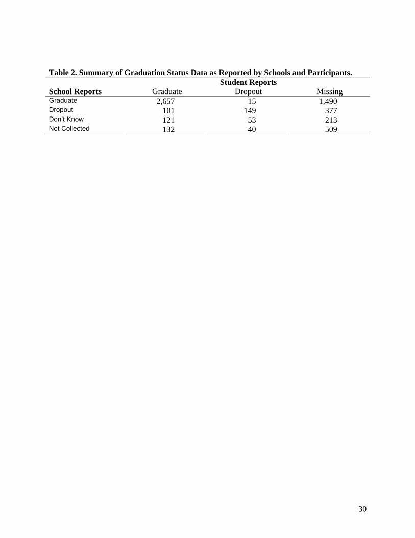
The dependent variable, high school dropout status, was collected through both school

administrative records and student self-reports. School-reported graduation data is missing for

301 students who moved from South Dakota before completing high school and for another 387

students for whom the South Dakota high schools reported graduation status was unknown.

Self-reported graduation status is missing for participants who failed to complete the post-high

school follow-up (n=2560) or completed the survey but failed to report high school graduation

status (n=29). The two data sources disagree with each other for some students. In particular, of

the students the school data reported as dropouts, 40% of the students who provided self-reported

status reported graduating. Hence, as discussed in the next section, we develop a model for the

join distribution of student and school-reported graduation status that allows for measurement

error in both.

Building on previous work demonstrating the importance of differentiating light and

heavy marijuana use (Chatterji, 2006; Roebuck et al., 2004; Ellickson et al., 1998;Yamada et al.,

1996), we construct a dichotomous measure of heavy and persistent marijuana use that equals

one if the student reports using marijuana three or more times in the past month on both the 9th

and 10th grade surveys and zero otherwise.

11

The following background, attitudinal and behavioral grade 7 control variables capture

the constructs represented in W: student demographics; family characteristics; school grades and

academic expectations; impulsivity; beliefs about the health consequences of alcohol, cigarette,

and marijuana use; parental monitoring; deviance; rates of time preference; religiosity; school

bonds; parental bonds; emotional distress; family (parent/sibling) substance use; and alcohol,

cigarette, and marijuana use in grade 7. We also control for peer effects for alcohol and cigarette

use, school size, region of the state, and the school’s experimental condition for the drug

prevention trial. 2 Because the sample is not perfectly balanced once we construct these

propensity score weights, we include some of these measures in the regression analyses in

addition to later measures of some of the same constructs (e.g. deviance in grades 8, 9 and 10;

substance use in grades 8, 9 and 10). Next, we discuss how these constructs are measured.

Unless otherwise noted, measures are created at grades 7 to 10 using parallel items; the grade 7

measure are included in the propensity score weights and measures from later grades are used in

sensitivity analyses.

Cigarette use is the logarithm of the 30 day average of one plus an overall frequency

index combining lifetime, past year, and past month frequency of use scaled by the student’s

quantity of use.3 Alcohol use is represented by categorical indicators measuring the number of

days of alcohol use in the past month, with levels of use indicated by none, 1, 2 to 4 days, 5 to 8

days, and 9 or more days (the reference group).

Deviance is the average frequency of six items tapping various deviant behaviors in each

grade (e.g. skipped school or breaking into houses, schools or places of business). To

2 Research suggests that by including all of these variables we risk potentially introducing greater variance into our estimate (and hence are more likely to reject the finding of significance), but the alternative is introducing bias caused by omitting relevant variables (Rubin, 1997; Rubin and Thomas, 1996). 3 The measure can be negative or positive (the minimum value is ln(1/30)=-3.4), because it uses the logarithm of index values that are both less than or greater than 1.

12

accommodate developmental change in the forms of deviant behavior, we added three additional

items to the grade 10 deviance index.4 The student’s rate of time preference is measured in

grades 7 and 9 as the sum of two items: How much of the time do you do or feel the following

things: you do what feels good now without thinking about the future, and you focus on the short

run instead of the long run (range = 0 (never) – 5 (almost always)).

Grade-specific measures of family influences on student behavior are based on two items:

whether the respondent perceives the adult they are closest to has a drinking habit and the extent

to which their parents would disapprove of them smoking or using marijuana. Grade-specific

measures of peer effects are tapped through self-reports by the students regarding the frequency

with which they are with marijuana using peers and whether they think their best friend uses

marijuana.5

Student attitudes and beliefs about alcohol, cigarettes, and marijuana are based on three

positive and three negative items for each substance, with a higher score on either scale

indicating more pro-drug attitudes. Indicators of bonds with conventional institutions are

captured through a measure of religiosity, school bonds, and parental bonds.6 Details regarding

the constructs of each of these can be found in Ellickson et al. (2003). Finally, we measured

emotional distress with the six-item mental health inventory index (MHI-6) that equals the MHI-

5 (Wells et al., 1996) plus an additional item on the frequency of feeling downhearted and blue

in past month. See Table 1 for descriptive statistics on all these variables.

4 Additional items are question regarding how often during the past year the student: ran away from home for a night or more; stole or tried to steal items worth $50 or more; sold marijuana; sold other drugs; took a vehicle for a joyride without the owner’s permission; drove a car, motorcycle or other vehicle after drinking alcohol; used strong-arm force to get money of things from people; attacked someone with the idea of seriously hurting or killing that person; purposely set fire or tried to set fire to a building, car, or other property; got into trouble with the police because of something you did. 5 The original scales for the two items combined for the peer measures differ so the items are standardized to mean zero and standard deviation one prior to being averaged for the index. Hence the index takes on both positive and negative values, with higher values on this index indicating more exposure to peer-using friends. 6 Religiosity was not measures at grade 7.

13

Table 1 here

Attrition and missing data. The data set includes 4,375 students with both marijuana use

and high school dropout data, which excludes 718 cases without graduation information from

either source and 764 students without marijuana use at either grade 9, grade 10 or both grades.

To account for attrition, we weighted the observations using propensity score based nonresponse

weights (Little and Rubin, 2002). In this case the propensity score represents the probability that

a student with a given set of baseline covariate values answered the 9th and 10th grade survey

questions on past month marijuana use and had data on graduation status. Nonresponse weights

equal the inverse of this probability for responding students. Missing data for baseline covariates

are imputed using a Bayesian model for the joint distribution of all baseline and 8th grade follow-

up variables.7 For data from the 9th and 10th grade follow-ups, missing values of independent

variables other than marijuana use are also imputed using a Bayesian model for the just

distribution of all analysis variables.

IV. Empirical Specification

As shown in Table 2, graduation information collected through self-reports did not

always match school administrator reports. To account for potential errors in reported

graduation status and make efficient use of the two incomplete data sources, we fit a model for

the joint distribution of student and school reported graduation status that allows for

measurement error in both. Given our structural model, we assumed a logistic regression model

for the true but not necessarily observed dropout status, DO = DO1HPMU + DO0 (1-HPMU),

7 The Bayesian imputation model uses a multivariate Gaussian distribution to approximate the joint distribution for the variables conditional on the unobserved parameter values. The imputed values are a random sample from the posterior distribution of the missing data and conditional on the observed data and the model. Using the NORM software (Schafer, 1999), we sampled five sets of imputed values. Imputed values have been found to be robust to model misspecifications (Schafer, 1997).

14

(4) P(DO = 1 | x, HPMU) = eα+β’x+γ HPMU/(1+ eα+β’x +γ HPMU)

The model also assumes that both school and student reports of graduation status might

contain errors. The error rates were specified through the conditional distribution of self-

reported status, U, given the true status, DO, and the conditional distribution of the school

reported status, Z, given DO. These were

(5) P(U = 1 | DO=1) = 1

(6) P(U = 1 | DO=0) = ε1

(7) P(Z = 1 | DO=1) = 1- ε2

(8) P(Z = 1 | DO=0) = ε2

Equation (5) assumes that high school graduates never incorrectly reported dropping out.

Equation (6) states that dropouts might self-report graduating with an error rate of ε1. Equations

(7) and (8) allow for errors in school reports and assume that false reports of dropout for

graduates and false reports of graduation for dropouts are equal.

Limited write-in data suggest that some students who had completed alternative

education programs mistakenly reported graduating from high school. We assumed that students

who had truly graduated from high school provided the correct information because there is no

obvious potential source of confusion that would result in misreporting graduation when it truly

occurred. We also assumed that students who reported dropping out provided the correct

information because there is no clear motivation for students to purposely misreport dropping out

(such as avoiding stigma or providing a socially desirable outcome) and because many students

who reported dropping out supplied reasons. Equations (7) and (8) are consistent with the

assumption that errors in school reporting are due to clerical mistakes, so that errors in either

direction have an equal probability of occurring.

15

Table 2 here

The model also assumes that U and Z are independent conditional on DO, which implies

that the errors made by schools are independent of errors by students. Given that the likely

sources of error in student and school reports are distinct this last assumptions seems reasonable.

Equations (4) – (8) yield

(9) P(U = u, Z = z | x, HPMU) = HPMUx

zzuuzzHPMUx

eue

γβα

γβα εεεεεε++

−−−++

+

−−+−'

)1(22

)1(112

)1(2

'

1)1()1()1(

.

From Equation (9), we derived a pseudo log-likelihood function for the observed pairs of

(U, Z), weighted by the propensity scores weights, to obtain estimates of (β, ε1, and ε2). We

estimated standard errors for the parameter estimates using a cluster adjusted sandwich estimator

(Liang and Zeger, 1986) based on the weighted pseudo log-likelihood function. To account for

the imputation of predictor variables, we repeated the estimation of parameters and standard

errors with each of the five imputation completed datasets and combined the resulting estimates

using standard methods (Schafer, 1997).8

IV. Results

Figure 1 demonstrates the balance between variable distributions for the HPMU and other

students in terms of the absolute standardized bias for the each pre-existing variable controlled in

our analysis. For each variable, the absolute standardized bias equals the absolute value of the

difference in the mean for the marijuana users and the (weighted) mean for other students

divided by the standard deviation for the marijuana users. If the groups are comparable these

8 We tested model specification by allowing the probability of errors in student self-reported data to depend

on student variables and using alternative probit link functions. The results were qualitatively invariant to the model; consequently, we report the results from the parsimonious model of Equation (9) rather than alternatives.

16

values should be close to zero. Values of greater than 0.25 are often considered problematic (Ho

et al., 2007).

Figure 1 here

As shown in the figure the groups differed substantially on many variables before

weighting for baseline differences in observable characteristics, with the absolute standardized

bias being greater than 0.2 for the majority of variables and being over 0.5 for 12 percent of the

variables. After weighting, the largest absolute standardized bias is just over 0.2 and only eight

differences are significant. Given the differences in baseline even after weighting, we include

variables with large differences (greater than 0.2) in our high school dropout equation after

weighting to further reduce the potential for biases in our findings. We also explored alternative

specifications with additional pre-existing variables included in the logistic regression model for

dropout to ensure that our results could not be explained by residual differences between the

groups on the pre-existing variables.

Table 3 presents results from our baseline models that evaluate the impact of persistent

marijuana use during grades 9 & 10 on high school dropout status. Model 1, which accounts

only for attrition (using nonreponse weights), yields a statistically significant nearly six-fold

increase in the odds of high school dropout for persistent marijuana users than nonusers or casual

users, and the finding is statistically significant. Model 2 shows that when we also account for

differences in baseline characteristics between persistent marijuana users and nonusers by

incorporating the propensity score weights, marijuana use remains statistically significant but it

is now associated with just over a 2.3 fold increase in the odds of dropout. If we can assume

strong ignorability, then we can conclude that heavy and persistent marijuana use increases the

risk of high school dropout.

17

Table 3 here

To test the strong ignorability assumption, we explore the effect of adding

contemporaneous measures of substance use that might share common unobservables with

marijuana use (Models 3 and 4). Because students who use marijuana are more likely to drink

alcohol (Gfroefer et al., 2002) and drinking can cause cognitive impairments and affect high

school graduation (Cook and Moore, 1993), we first consider alcohol, Including days of alcohol

use during grades 8 through 10 does not change the marijuana results qualitatively. In fact, the

odds ratio on persistent marijuana use actually increases. Next, we consider cigarettes (Model

4). Unlike alcohol, there is no physiological reason why cigarette smoking would affect school

performance or dropout status, as smoking is not known to impair cognitive functioning nor is it

known to offset the deleterious effects on cognitive functioning associated with marijuana use.

However, numerous studies have shown that smoking is a strong predictor of marijuana use

(Gfroefer et al., 2002; Ellickson et al., 1998; Sommer, 1985). Model 4 shows that including

cigarette smoking in grades 8 through 10 causes a substantial reduction in the magnitude and our

marijuana use measure, which is no longer a statistically significant predictor of high school

dropout status.

If heavy and persistent marijuana use was only associated with high school dropout

because of its impact on cognitive functioning, then including cigarette use in our regression

model should have no impact on the coefficient (or odds ratio) on marijuana use. The fact that it

does suggests that the association is largely generated by an omitted variable bias. Recall that

the propensity score weights are constructed using variables representing a wide range of

constructs previously reviewed, but the constructs are all measured at baseline (Grade 7 or 8). If

18

the influence of particular constructs changes over time, then baseline corrections will be

insufficient to represent them.

Models 5 and 6 evaluate whether the omitted variable bias is caused by lack of controls

for school performance. School performance measures, such as grades, are presumed to impact

the likelihood of completing high school but may also be directly affected by marijuana use, so

we intentionally excluded them from previous analyses to reduce endogeneity bias. Model 5

shows that including grades in the 8th, 9th and 10th grade, while significantly influencing the

likelihood of dropping out, has only a small impact on the estimated effect of marijuana use.

When school grades are included (Model 5), the odds ratio for marijuana falls slightly but

remains statistically significant. When cigarette use is included with grades (Model 6), the odds

ratio for marijuana use drops substantially and is no longer significant but cigarette use continues

to have a positive impact on high school dropout status.

Table 4 provides the results of sensitivity analyses that explore the impact of probable

sources of the relationship between marijuana use and dropout that cigarettes use might be

representing. In the first row, we include three separate indices of deviance in grades 8, 9 and

10, finding that the odds ratio for marijuana use is reduced but remains statistically significant

unless cigarettes are also included (row 2). Indices of the student’s bonds to social institutions

(religious and school) in grades 8, 9 and 10 also do not account for the relationship between

marijuana use and high school dropout. The odds ratio in this specification (Row 3) remains

greater than 2 and statistically significant, unless cigarette use is also added (Row 4). We get the

exact same findings when we add rates of time preference (Rows 5 & 6), emotional distress

(Rows 7 & 8) and family stress (Rows 9 & 10). Including attitudes toward drugs yields a

somewhat larger drop in the odds ratio for marijuana use (Row 11), although the odds ratio is

19

statistically significant at the 6% level and only becomes completely insignificant when

measures of cigarette use are included (Row 12). In Rows 13 and 15, we finally identify two

factors that explain the relationship between marijuana use and dropout: family influence and

peer effects in grades 8, 9 or 10. When these indices are included (without cigarette use),

marijuana use has a much smaller odds ratio and is no longer a significant predictor of high

school dropout status. Cigarette use is significant when it is also included (Rows 14 & 16),

Table 4 here

V. Discussion and Conclusions

A number of interesting conclusions can be drawn from these results. First, the Table 3

results indicate that important differences in baseline characteristics exist between individuals

who choose to use marijuana and those who do not, even before most of these individuals ever

initiate marijuana. Ignoring the selectivity bias indicated by these differences can lead to a

significant over-estimation of the association between marijuana use and schooling. Once we

accounted for these baseline differences using propensity score weights, the odds ratio on

marijuana use was cut in half, although still quite large and statistically significant.

Second, the results in Tables 3 and 4 indicate that the remaining relationship between

marijuana use and dropout does not reflect a causal effect on cognitive functioning. The odds-

ratio for marijuana use is greatly reduced and no longer statistically significant after we control

for the students’ grade 9 and 10 cigarette smoking. There are three potential interpretations of

this result. First, marijuana use causes cigarette smoking and controlling for smoking in the

model is inducing a negative bias on the coefficient for marijuana use. This interpretation,

however, is not supported by scientific evidence. We are not aware of any scientific evidence

20

showing that cigarette use has an independent and direct negative effect on cognition; moreover,

controlling for grades has almost no effect on the odd-ratio for marijuana use.

The second possible interpretation of the cigarette result is that there is common

unexplained heterogeneity among students who smoke marijuana and cigarettes and including

cigarette use in the model results in negative endogeneity bias in the odd-ratio for marijuana use.

A negative endogeneity bias requires that, conditional on these unobserved factors for smoking,

students with greater unobserved risks for marijuana use have smaller risks for dropout. This

seems unlikely. In all observed data from our study and many other studies, youth who use

marijuana have greater risk factors for negative behaviors and outcomes including negative peer

associations, weak social bonds, low aspirations, and increased deviant behaviors. While we

cannot rule out the possibility that unobserved heterogeneity creates a situation where

conditioning on smoking reverses the strong relationship between marijuana use and negative

risk factors, this sort of endogeneity bias seems much less likely than omitted-variable bias

between marijuana use and dropout.

The third potential explanation, that the relationship between marijuana use and dropout

is attributable to omitted bias arising from a failure to fully account for pre-existing differences

between students who use marijuana in grades 9 and 10 and those who do not, is the most

defensible. Cigarette smoking is known to be correlated with multiple demographic and

psychosocial risk factors for negative outcomes (Collins and Ellickson, 2004; Tucker et al.,

2006). In this study, two other risk factors, peer associations and family influences, also

accounted for the relationship between marijuana use and dropout. Although peer associations

could be endogenous and causally influenced by marijuana use, this should be less true of family

influences.

21

We also note that controlling for a rich set of variables at grade seven was not sufficient

to control for the dynamic changes that occur during adolescence and that result in students who

are similar at grades 7 and 8 choosing to (or not to) engage in heavy and persistent marijuana use

during grades 9 and 10. The unobserved differences then persist, creating differential risks for

dropout and a spurious relationship between marijuana and dropout even conditional on the

baseline data.

When interpreting the above results, two study limitations should be kept in mind. First,

we examine student behaviors in only one state, South Dakota. Because South Dakota is very

rural, with only two major cities, this sample may not accurately reflect the experience of all U.S.

students. Second, inherent measurement error or possible limitations in our measurement of

specific baseline constructs could partially explain the insufficiency of baseline measures to

remove differences between marijuana users and other students that contribute to differences in

dropout rates. In other words, there may still be unobservable factors biasing our results.

Nonetheless, the results presented here show that the negative association between

marijuana use and high school completion cannot be viewed as causal. Instead, our findings

suggest that this association is generated by a spurious correlation with unobserved factors that

change in significant ways during early adolescence, which reduces the ability of traditional

econometric methods to adequately account for them. We cannot conclude that marijuana use

has no deleterious effect on cognitive functioning. This study does not directly assess the affect

of marijuana on cognitive ability. Instead, it examines an outcome that represents a cumulative

decision based on a variety of factors, including ability, school performance, institutional

bonding, peer effects, attitudes, and economic status. What this study does suggest is that the

positive association that has been frequently interpreted as a causal effect instead reflects a

22

common shared association with other time persistent and time varying factors that frequently

get omitted from economic studies examining this relationship.

In addition to the contributions regarding the importance and nature of time variant

unobserved heterogeneity, this study also provides insights regarding appropriate instruments

when trying to identify causal associations using instrumental variables techniques. Our results

show that measures of cigarette use, peer substance use and parental substance use, which have

been used in previous analyses, would be poor instruments as they are heavily correlated with

high school completion as well as marijuana use.

23

References

Bandura A. 1985. Social Foundations of Thought and Action. Prentice Hall: Englewood Cliffs,

NJ.

Bandura A. 1977. Self-efficacy: toward a unifying theory of behavioral change. Psychological

Review 84: 191-215.

Barnes G.E., Barnes M.D., Patton, D. 2005. Prevalence and predictors of “heavy” marijuana

use in a Canadian sample” Journal of Substance Use and Misuse 40: 1849-1863.

Bailey S.L., Hubbard R.L. 1990. Developmental variation in the context of marijuana

initiation among adolescents. Journal of Health and Social Behavior 31: 58-70.

Bang H., Robins, J.M. 2005. Doubly robust estimation in missing data and causal inference

models. Biometrics 61: 962-973

Bray J. W., Zarkin G.A., Ringwalt C., Qi J. 2000. The Relationship between marijuana initiation

and dropping out of high school. Health Economics 9: 9-18.

Brook J.S., Balka E.B., Whiteman M. 1999. The risks for late adolescence of early adolescent

marijuana use. American Journal of Public Health, 89: 1549-54.

Chatterji, P. 2006. Illicit drug use and educational attainment. Health Economics 15: 489- 511.

Collins R.L., Ellickson P.L. 2004. Integrating four theories of adolescent smoking.

Substance Use and Misuse 39: 179-209.

Cook P.J., Moore, M.J. 1993. Drinking and schooling. Journal of Health Economics 12: 411-

429.

Donovan J.E., Jessor R. 1985. Structure of problem behavior in adolescence and young

adulthood. Journal of Consulting and Clinical Psychology, 53: 890-904.

24

Duncan S.C., Duncan T.E., Biglan A., Ary D. 1998. Contributions of the social context to the

development of adolescent substance use: a multivariate latent growth modelling approach.

Drug and Alcohol Dependence, 50: 57-71.

Ellickson P. K. Bui K., Bell R., McGuigan K.A.1998. Does early drug use increase the risk of

dropping out of high school? Journal of Drug Issues 28: 357-380.

Ellickson P.L., McCaffrey D.F., Ghosh-Dastidar B., Longshore D. 2003. New inroads in

preventing adolescent drug use: results from a large-scale trial of project ALERT in

middle schools. American Journal of Public Health 93: 1830-1836.

Farrell P., Fuchs V.R. 1982. Schooling and health: the cigarette connection. Journal of Health

Economics 1: 217-30.

Fergusson D.M., Horwood L.J. 1997. Early onset cannabis use and psychosocial adjustment in

young adults. Addiction 92: 279-96.

Fergusson, D.M., Horword L.J., Swain-Campbell N. 2002. Cannabis use and psychosocial

adjustment in adolescence and young adulthood. Addiction 97: 1123-35.

Fergusson D.M., Lynskey M.T., Horwood L.J. 1996. The short-term consequences of early

onset cannabis use. Journal of Abnormal Child Psychology 24: 499-512.

Fuchs V.R. 1982. Time preference and health: An exploratory study. In: FUCHS, V.R., ed.

Economic Aspects of Health. Chicago, IL: University of Chicago Press for National

Bureau of Economic Research, pp. 93-120.

Gfroerer J.C., Wu L.T., Penne M.A. 2002. Initiation of Marijuana Use: Trends, Patterns, and

Implications (Analytic Series: A-17, DHHS Publication No. SMA 02-3711). Rockville,

MD: Substance Abuse and Mental Health Services Administration, Office of Applied

Studies.

25

Grossman M. 1972. On the concept of health capital and the demand for health. Journal of

Political Economy 80: 223-255.

Hawkins J.D., Catalano R.F., Miller J.Y. 1992. Risk and protective factors for alcohol and other

drug problems in adolescence and early adulthood: implications for substance abuse

prevention. Psychological Bulletin, 112: 64-105.

Hawkins J.D., Weis J.G. 1985. The social development model: An integrated approach to

delinquency prevention. Journal of Primary Prevention 6: 73-97.

Heyser C. J., Hampson R.E., Deadwyler S.A. 1993. Effects of Delta-9-Tetrahydrocannabinol on

delayed match to sample performance in rats: alterations in short-term memory

associated with changes in task specific firing of hippocampal cells. The Journal of

Pharmacology and Experimental Therapeutics 264: 294-307.

Ho D., Imai K., King G., Stuart E.A. 2007. Matching as nonparametric preprocessing for

reducing model dependence in parametric causal inference. Political Analysis, 15: 199-

236.

Jessor R., Jessor S.L. 1977. Problem Behavior and Psychosocial Development: A Longitudinal

Study of Youth, New York: Academic Press.

Kumar R, O’Malley P.M., Johnston L.D., Schulenberg, J.E., Bachman J.G. 2002. Effects of

school-level norms on student substance use. Prevention Science 3: 105-124.

LaGrange, R.L., White H.R. 1985. Age differences in delinquency: a test of theory.

Criminology 23: 19-45.

Liang K.Y., Zeger S.L. 1986. Longitudinal data analysis using generalized linear models.

Biometrika 73: 13-22.

26

Little R.J.A., Rubin D.B. 2002. Statistical Analysis with Missing Data. New York: John Wiley &

Sons.

Matsuda L.A., Bonner T.I., Lolait S.J. 1993. Localization of cannabinoid receptor messenger

RNA in rat brain. Journal of Comparative Neurology 327: 535-550.

Mensch B.S., Kandel D.B. 1988. Dropping out of high school and drug involvement.

Sociology of Education 61: 95-113.

Mendelson, J., Rossi M., Meyer R. 1974. The Use of Marihuana: A Psychological and

Physiological Inquiry, New York: Plenum.

Newcomb M, Bentler P. 1986. Drug use, educational aspirations, and work force involvement:

the transition from adolescence to young adulthood. American Journal of Community

Psychology 14: 303-321.

Newcomb M, Bentler P. 1988. Consequences of Adolescent Drug Use: Impact on the Lives of

Young Adults. Newbury Park, CA: Sage Publications.

Ridgeway G., McCaffrey D.F. 2007. Comment: demystifying double robustness: a comparison

of alternative strategies for estimating a population mean from incomplete data.

Statistical Science 22: 540-543.

Roebuck M.C., French M.T., Dennis M.L. 2004. Adolescent marijuana use and school

attendance. Economics of Education Review 23: 133-141.

Rosenbaum P.R., Rubin D.B. 1983. The central role of the propensity score in observational

studies for causal effects. Biometrika 70: 41-55.

Rubin D.B. 1997. Estimating causal effects from large data sets using propensity scores. Annals

of Internal Medicine 127: 757-176.

27

Rubin D.B., Thomas N. 1996. Matching using estimated propensity scores: relating theory to

practice. Biometrika 52: 249-264.

Sander W. 1998. The effects of schooling and cognitive ability on smoking and marijuana use by

young adults. Economics of Education Review 17: 317-324.

Schafer J.L. 1997. Analysis of Incomplete Multivariate Data by Simulation. New York:

Chapman & Hall Ltd.

Schafer J.L. 1999. Software for multiple imputation. www.stat.psu.edu/~jls/misoftwa.html [May

26, 2008].

Schulenberg J., Bachman J.G., O'Malley P.M., Johnston L.D. 1994. High school educational

success and subsequent substance use: a panel analysis following adolescents into young

adulthood. Journal of Health and Social Behavior 35: 45-62.

Simmons R.G., Blyth D.A. 1987. Moving into Adolescence: The Impact of Pubertal Change and

School Context. New York: Aldine de Gruyter.

Sommer B. 1985. Truancy in early adolescence. Journal of Early Adolescence, 5: 145–160.

Tucker J.S., Ellickson P.E., Orlando M., Klein D.J. 2006. Cigarette smoking from

adolescence to young adulthood: women’s developmental trajectories and

associated outcomes. Women’s Health Issues 16: 30-37.

Wells K.B., Sturm R., Sherbourne C.D., Meredith L.S. 1996. Caring for Depression. Cambridge

MA: Harvard University Press.

Wills T.A., Shiffman S. 1985. Coping and substance use: a conceptual framework. In WILLS

T.A., SHIFFMAN S., eds. Coping and Substance Use Orlando FL: Academic Press, pp.

3-24.

28

Yamada T., Kendix M., Yamada T. 1996. The impact of alcohol consumption and marijuana use

on high school graduation. Health Economics 5: 77-92.

29

Table 1. Summary Statistics for Analysis Variables

Variable Mean Standard Deviation Variable Mean

Standard Deviation

Persistent Marijuana Use (Gr 9 & 10) 0.072 0.259 Deviance, Gr 8 0.418 0.597 Age 12.348 0.499 Deviance, Gr 9 0.483 0.665 Female 0.509 0.500 Deviance, Gr 10 0.281 0.393 Race/Ethnicity Social Bonds White 0.900 0.300 Religiosity, Gr 8 2.330 1.008 Native American 0.058 0.234 Religiosity, Gr 9 2.577 1.044 Other Race 0.041 0.198 Religiosity, Gr 10 2.641 1.086 Mother's Education 1.846 0.957 School Bonds, Gr 8 2.255 0.621 Father’s Education 1.958 1.002 School Bonds, Gr 9 2.285 0.649 Nuclear Family 0.735 0.442 School Bonds, Gr 10 2.359 0.643 Experimental Condition Family Bonds, Gr 8 1.799 0.726 Contrl 0.348 0.476 Family Bonds, Gr 9 1.813 0.815 ALERT Only 0.318 0.466 Family Bonds, Gr 10 1.881 0.838 ALERT Plus 0.333 0.471 Time Preference, Gr 9 1.112 0.982 Days Alone After School, Gr 7 2.702 1.826 Emotional Distress, Gr 8 1.355 0.848 Hours Alone After School, G. 7 2.763 1.538 Emotional Distress, Gr 9 1.517 0.938 Alcohol Consequence, Gr 7 0.047 0.195 Emotional Distress, Gr 10 1.561 0.938 Peer Alc Use, Gr 7 -0.090 0.751 Attitudes Used Cigs in Past Month, Gr 7 0.079 0.27 Positive Attitudes, Gr 8 1.586 0.853 Low Resistence-Self Efficacy to Substance Use at Parties 1.428 0.677 Positive Attitudes, Gr 9 1.868 1.017 Peer Pot Use, Gr 7 -0.118 0.641 Positive Attitudes, Gr 10 2.155 1.049 Used Alcohol 0 Days in Past Month, Gr 8 0.695 0.460 Negative Attitudes, Gr 8 1.484 0.837 Used Alcohol 1 Day in Past Month, Gr 8 0.181 0.385 Negative Attitudes, Gr 9 1.661 0.95 Used Alcohol 2-4 Days in Past Month, Gr 8 0.080 0.271 Negative Attitudes, Gr 10 1.895 0.995 Used Alcohol 5-8 Days in Past Month, Gr 8 0.034 0.181 Family Influences Used Alcohol 9+ Days in Past Month, Gr 8 0.010 0.099 Adult Use Cig, Gr 8 0.922 1.322 Used Alcohol 0 Days in Past Month, Gr 9 0.573 0.495 Adult Use Cig, Gr 9 0.910 1.327 Used Alcohol 1 Day in Past Month, Gr 9 0.210 0.407 Adult Use Cig, Gr 10 0.875 1.313 Used Alcohol 2-4 Days in Past Month, Gr 9 0.127 0.333 Parental Approval Cig, Gr 8 1.326 0.647 Used Alcohol 5-8 Days in Past Month, Gr 9 0.071 0.257 Parental Approval Cig, Gr 9 1.475 0.765 Used Alcohol 9+ Days in Past Month, Gr 9 0.019 0.137 Parental Approval Cig, Gr 10 1.634 0.87 Used Alcohol 0 Days in Past Month, Gr 10 0.501 0.500 Parental Approval Pot, Gr 8 1.088 0.371 Used Alcohol 1 Day in Past Month, Gr 10 0.216 0.412 Parental Approval Pot, Gr 9 1.149 0.488 Used Alcohol 2-4 Days in Past Month, Gr 10 0.157 0.364 Parental Approval Pot, Gr 10 1.257 0.626 Used Alcohol 5-8 Days in Past Month, Gr 10 0.100 0.300 Peer Efffects, Gr 8 0.299 0.538 Used Alcohol 9+ Days in Past Month, Gr 10 0.025 0.156 Peer Efffects, Gr 9 0.583 0.757 Gr 8: Freq Cig Use -2.949 1.171 Peer Efffects, Gr 10 0.782 0.828 Gr 9: Freq Cig Use -2.638 1.593 Divorce, Gr 10 0.171 0.376 Gr 10: Freq Cig Use -2.375 1.853 Family Stresses, Gr 10 0.250 0.433 Grades in Gr 8 1.865 0.897

Grades in Gr 9 1.944 0.942

Grades in Gr 10 1.951 0.932

30

Table 2. Summary of Graduation Status Data as Reported by Schools and Participants. Student Reports School Reports Graduate Dropout Missing Graduate 2,657 15 1,490 Dropout 101 149 377 Don’t Know 121 53 213 Not Collected 132 40 509

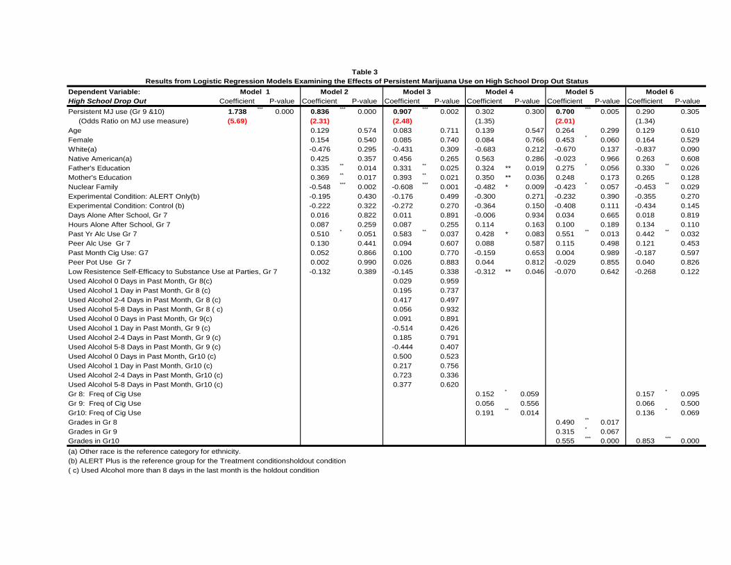
Table 3Results from Logistic Regression Models Examining the Effects of Persistent Marijuana Use on High School Drop Out Status

Dependent Variable: Model 1 Model 2 Model 3 Model 4 Model 5 Model 6High School Drop Out Coefficient P-value Coefficient P-value Coefficient P-value Coefficient P-value Coefficient P-value Coefficient P-valuePersistent MJ use (Gr 9 &10) 1.738 *** 0.000 0.836 *** 0.000 0.907 *** 0.002 0.302 0.300 0.700 *** 0.005 0.290 0.305 (Odds Ratio on MJ use measure) (5.69) (2.31) (2.48) (1.35) (2.01) (1.34)Age 0.129 0.574 0.083 0.711 0.139 0.547 0.264 0.299 0.129 0.610Female 0.154 0.540 0.085 0.740 0.084 0.766 0.453 * 0.060 0.164 0.529White(a) -0.476 0.295 -0.431 0.309 -0.683 0.212 -0.670 0.137 -0.837 0.090Native American(a) 0.425 0.357 0.456 0.265 0.563 0.286 -0.023 0.966 0.263 0.608Father's Education 0.335 ** 0.014 0.331 ** 0.025 0.324 ** 0.019 0.275 * 0.056 0.330 ** 0.026Mother's Education 0.369 ** 0.017 0.393 ** 0.021 0.350 ** 0.036 0.248 0.173 0.265 0.128Nuclear Family -0.548 *** 0.002 -0.608 *** 0.001 -0.482 * 0.009 -0.423 * 0.057 -0.453 ** 0.029Experimental Condition: ALERT Only(b) -0.195 0.430 -0.176 0.499 -0.300 0.271 -0.232 0.390 -0.355 0.270Experimental Condition: Control (b) -0.222 0.322 -0.272 0.270 -0.364 0.150 -0.408 0.111 -0.434 0.145Days Alone After School, Gr 7 0.016 0.822 0.011 0.891 -0.006 0.934 0.034 0.665 0.018 0.819Hours Alone After School, Gr 7 0.087 0.259 0.087 0.255 0.114 0.163 0.100 0.189 0.134 0.110Past Yr Alc Use Gr 7 0.510 * 0.051 0.583 ** 0.037 0.428 * 0.083 0.551 ** 0.013 0.442 ** 0.032Peer Alc Use Gr 7 0.130 0.441 0.094 0.607 0.088 0.587 0.115 0.498 0.121 0.453Past Month Cig Use: G7 0.052 0.866 0.100 0.770 -0.159 0.653 0.004 0.989 -0.187 0.597Peer Pot Use Gr 7 0.002 0.990 0.026 0.883 0.044 0.812 -0.029 0.855 0.040 0.826Low Resistence Self-Efficacy to Substance Use at Parties, Gr 7 -0.132 0.389 -0.145 0.338 -0.312 ** 0.046 -0.070 0.642 -0.268 0.122Used Alcohol 0 Days in Past Month, Gr 8(c) 0.029 0.959Used Alcohol 1 Day in Past Month, Gr 8 (c) 0.195 0.737Used Alcohol 2-4 Days in Past Month, Gr 8 (c) 0.417 0.497Used Alcohol 5-8 Days in Past Month, Gr 8 ( c) 0.056 0.932Used Alcohol 0 Days in Past Month, Gr 9(c) 0.091 0.891Used Alcohol 1 Day in Past Month, Gr 9 (c) -0.514 0.426Used Alcohol 2-4 Days in Past Month, Gr 9 (c) 0.185 0.791Used Alcohol 5-8 Days in Past Month, Gr 9 (c) -0.444 0.407Used Alcohol 0 Days in Past Month, Gr10 (c) 0.500 0.523Used Alcohol 1 Day in Past Month, Gr10 (c) 0.217 0.756Used Alcohol 2-4 Days in Past Month, Gr10 (c) 0.723 0.336Used Alcohol 5-8 Days in Past Month, Gr10 (c) 0.377 0.620Gr 8: Freq of Cig Use 0.152 * 0.059 0.157 * 0.095Gr 9: Freq of Cig Use 0.056 0.556 0.066 0.500Gr10: Freq of Cig Use 0.191 ** 0.014 0.136 * 0.069Grades in Gr 8 0.490 ** 0.017Grades in Gr 9 0.315 * 0.067Grades in Gr10 0.555 *** 0.000 0.853 *** 0.000(a) Other race is the reference category for ethnicity.(b) ALERT Plus is the reference group for the Treatment conditionsholdout condition( c) Used Alcohol more than 8 days in the last month is the holdout condition

32

Table 4:Sensitivity Analyses Examining the Effects of Persistent Marijuana (MJ) Use on High School Dropout Statusa

Odds Ratio Odds RatioModel Model Specification Persistent MJ Use P-value Gr 10 Cig Use P-value

1 Deviance (Gr 8 - Gr 10) 1.948 ** 0.0162 Deviance + Cigarettes (Gr 8 - Gr 10) 1.280 0.430 1.208 *** 0.0033 Social Bonds (Gr 8 - Gr 10) 2.157 *** 0.0034 Social Bonds + Cigarettes (Gr 8 - Gr 10) 1.312 0.374 1.209 *** 0.0025 Time Preference (Gr 9) 2.168 *** 0.0026 Time Preference (Gr 9) + Cigarettes (Gr 8 - Gr 10) 1.328 0.329 1.210 ** 0.0167 Emotional Distress (Gr 8 - Gr 10) 2.368 *** 0.0008 Emotional Distress + Cigarettes (Gr 8 - Gr 10) 1.348 0.300 1.211 ** 0.0189 Family Stresses + Divorce (Gr XX) 2.356 *** 0.00010 Family Stresses + Divorce (Gr XX) + Cigarettes (Gr 8 - Gr 10) 1.388 0.247 1.205 ** 0.00111 Attitudes (Gr 8 - Gr 10) 1.761 * 0.06212 Attitudes + Cigarettes (Gr 8 - Gr 10) 1.279 0.417 1.227 *** 0.00913 Family Influence (Gr 10) 1.422 0.23914 Family Influence (Gr 10) + Cigarettes (Gr 8 - Gr 10) 1.006 0.985 1.224 ** 0.02915 Peer Effects (Gr 8 - Gr 10) 1.296 0.41916 Peer Effects + Cigarettes (Gr 8 - Gr 10) 0.096 0.909 1.200 ** 0.045

a All models include as additional regressors, nonresponse weights, propensity score weights, and an indicator of treatment effect. Statistical significance is indicated as follows: *** indicates significance at the 1% level (two-tailed test), ** indicates significance at the 5% level (two-tailed test), * indicates significance at the 10% level (two-tailed test).

33

Figure 1

0.0

0.1

0.2

0.3

0.4

0.5

0.6

0.7

Abs

olut

e S

td D

iffer

ence

Unweighted Weighted

Figure 1. Comparison of HPMU and other students on covariates measured prior to HPMU measure before and after propensity score weighting. Dots represent the absolute standardized bias, the absolute value of the quantity of the difference in the mean for HPMU and other students divided by the standard deviation for the HPMU students, for each variable considered in the modeling, lines connect dot for the same variable with and without weighting solid dots denote statistically significant differences (p < 0.05)