maria kateri web-appendix of contingency table...
TRANSCRIPT
.
Maria Kateri
Web-Appendix of
CONTINGENCY TABLE ANALYSIS
Methods and Implementation Using R

Contents
Web Appendix: Contingency Table Analysis in Practice . . . . . . . . . . . . . . . . . 1A.1 Software for Categorical Data Analysis . . . . . . . . . . . . . .. . . . . . . . . . 1A.2 Contingency Table Analysis inR. . . . . . . . . . . . . . . . . . . . . . . . . . . . . . 2
A.2.1 R-Packages Useful in Contingency Table Analysis . . . . . . . . 2A.2.2 Data Input inR . . . . . . . . . . . . . . . . . . . . . . . . . . . . . . . . . . . . . . 4
A.3 R - Functions Used . . . . . . . . . . . . . . . . . . . . . . . . . . . . . . . . . . . . .. . . . 6A.3.1 R - Functions of Chapter 1 . . . . . . . . . . . . . . . . . . . . . . . . . . . . 6A.3.2 R - Functions of Chapter 2 . . . . . . . . . . . . . . . . . . . . . . . . . . . . 7A.3.3 R - Functions of Chapter 3 . . . . . . . . . . . . . . . . . . . . . . . . . . . . 12A.3.4 R - Functions of Chapter 5 . . . . . . . . . . . . . . . . . . . . . . . . . . . . 13A.3.5 R - Functions of Chapter 6 . . . . . . . . . . . . . . . . . . . . . . . . . . . . 15A.3.6 R - Functions of Chapter 9 . . . . . . . . . . . . . . . . . . . . . . . . . . . . 20
A.4 Contingency Tables Analysis in SPSS . . . . . . . . . . . . . . . . .. . . . . . . . 22A.4.1 Independence for Two-Way Tables Using SPSS MATRIX . . 22A.4.2 Association Models for Two-Way Tables in SPSS . . . . . . .. . 23A.4.3 Symmetry Models in SPSS . . . . . . . . . . . . . . . . . . . . . . . . . .. . 29


Appendix AWeb Appendix: Contingency Table Analysis inPractice
A.1 Software for Categorical Data Analysis
Standard statistical packages, such as SAS, SPSS, S-Plus, are well-supplied to treatcategorical data. Especially in their updated versions, their features concerning ca-tegorical data analysis are enriched. They incorporated procedures for applying therecent developed methods and models in categorical data analysis, following thenew computing strategies. Briefly, one could say that their major new features con-cern mainly options for exact analysis and analysis of repeated categorical data.Thus, LMIXED of SAS fits generalized linear mixed models while GEE analysisfor marginal models can be performed in GENMOD. The related gee() function isavailable in S-Plus. SPSS (version 15) offers the ‘Generalized Estimating Equations’sub-option under the ‘GLMs’ option of ‘Analyze’.
For SAS, a variety of codes are presented and discussed in theAppendix ofAgresti (2002, 2007). In S-Plus, for advanced models one hasto use special func-tions, developed individually and included in different libraries. Orientated towardcategorical data analysis and models for ordinal data as well, are the MASS library(Venables and Replay) and VGLM, VGAM, developed by Yee. For example, gen-eralized linear mixed models can be fitted through the glmmPQL() function of theMASS library.
Of increasing popularity and usage is the free software R, for statistical com-puting and graphics (R web site: http://www.r-project.org/). R language and envi-ronment is similar to S and code written for S runs usually under R as well. Manyresearchers support their published papers with the related R program. This way, Rsoftware is continuously updated and one can find a variety offunctions for basic oradvanced analysis of categorical data and special types of them.
Further on, BMDP, MINITAB, STATA and SYSTAT have all components forcategorical data inference and generalized linear models.Bayesian analysis of ca-tegorical data can be carried out through WINBUGS, which is a free software(http://www.mrc-bsu.cam.ac.uk/bugs/winbugs/contents.shtml). Another option is to
1

2 A. Web Appendix: Contingency Table Analysis in Practice
perform categorical data analysis through MATLAB, as by Johnson and Albert(2000). The MATLAB functions they used, are described in their Appendix.
For categorical data analysis, there have been developed also some special pack-ages. Thus, exact analysis of categorical data is performedby StatXact while exactconditional logistic regression can be fitted by LogXact. SUDAAN is specializedfor analysis of mixed data from stratified multi-stage cluster designs. It has also thefeature of analyzing marginal models for nominal and ordinal responses by GEE.Software tool for estimating marginal regression models isalso MAREG.
Finally, some algorithms may be found in Fortran. For example, Haberman(1995) provided a Fortran program for fitting the association model RC(K) by theNewton-Raphson method while Ait-Sidi-Allal et al. (2004) implemented their al-gorithms for estimating parameters in association and correlation models also inFortran.
A.2 Contingency Table Analysis in R
This section of the Appendix is not to be considered as a kind of manual forR.It is far from complete and, most important, this is not our intention. There isa big variety of books and on-line notes that serve this purpose. For an excel-lent, clear and short, introduction inR with emphasis on categorical data, we re-fer to Altham’s ‘Introduction to Statistical Modelling in R’, last updated in 2012(http://www.statslab.cam.ac.uk/ pat/redwsheets.pdf).This Appendix serves the pur-pose of making the book more comprehensive and of providing the opportunity toapply in practice all the discussed models, even the non-trivial ones, fast and readily.Of course, the way to use software is not unique and we do not claim that we pro-vide always the ‘best way’. We hope that we provide the easiest to follow approach,also for readers not familiar withR .
A.2.1 R-Packages Useful in Contingency Table Analysis
We provide next a collection (in alphabetical order) of special Rpackages, useful inthe analysis of contingency tables. Of course, the list is not exhaustive. Most of themare to be found inAvailable Packages at http://cran.r-project.org/web/packages/.
• ancor : Simple and canonical correspondence analysis (CA) on a two-way fre-quency table (with missings) by means of SVD (J. de Leeuw and P. Mair).
• boot : Bootstrap R (S-Plus) functions (A. Canty).• BradleyTerry2 : Bradley-Terry models (H. Turner and D. Firth).• ca : Simple, multiple and joint correspondence analysis (M. Greenacre and O.
Nenadic).• cat : Analysis of categorical-variable datasets with missing values (T. Harding
and F. Tusell).

A.2. Contingency Tables Analysis inR 3
• catspec : Special models for categorical variables.sqtab() estimates log-linear models for square tables such as quasi-independence, symmetry, uniformassociation (J. Hendrickx).
• cmm: Categorical marginal models (W. Bergsma and A. van der Ark).• cond : Approximate conditional inference for logistic and loglinear models (A.
R. Brazzale).• conting : Bayesian analysis of complete and incomplete contingencytables (A.
M. Overstall and R. King).• dixon : Nearest neighbour contingency table analysis (M. de la Cruz Rot and P.
M. Dixon).• exact2x2 : Exact conditional tests and confidence intervals for 2x2 tables (M.P.
Fay).• exactLoglinTest : Monte Carlo exact tests for log-linear models (B. Caffo).• FactoMineR : Multivariate exploratory data analysis and datamining inR; per-
forms also correspondence analysis (CA) and multiple CA (F.Husson, J.Jose, S.Le and J. Pages).
• foreign : Read data stored by Minitab, S, SAS, SPSS, Stata, Systat, dBase, ...(R Core team).
• gam: Generalized additive models (T. Hastie).• gllm : Generalised log-linear models; fits log-linear models on incomplete con-
tingency tables, including some latent class models (D. Duffy).• gnm: Generalized nonlinear models (H. Turner and D. Firth).• gRapHD: Designed for selecting high-dimensional undirected graphical models,
displaying their independence graphs and analysing graphical structures. It sup-ports the use of discrete, continuous, or both types of variables (G. de Abreu, R.Labouriau and D. Edwards).
• gRbase : A platform for graphical models in R, includes also functions for ma-nipulation of highdimensional tables (S. Hojsgaard and C. Dethlefsen).
• gRim: Graphical log-linear models for contingency tables, graphical Gaussianmodels for multivariate normal data, mixed interaction models (S. Hojsgaard).
• hmmm: A collection of functions for specifying and fitting marginal models (hi-erarchical multinomial marginal models), multinomial Poisson homogeneous(MPH) models and homogeneous linear predictor (HLP) modelsfor contingencytables (R. Colombi, S. Giordano, M. Cazzaro and J.B. Lang).
• MASS: Functions and datasets to support ’Modern Applied Statistics with S’ (4thedition, 2002) by Venables and Ripley.
• metafor : A package for conducting meta-analyses in R. For meta-analysesof 2x2 tables, specialized methods are implemented, including the the Mantel-Haenszel test and the Breslow-Day test with Tarone’s adjustment (W. Viecht-bauer).
• mlogit : multinomial logit model (Y. Croissant).• mlogitBMA : Bayesian model averaging for multinomial logit models (H.Sev-
cikova and A. Raftery).

4 A. Web Appendix: Contingency Table Analysis in Practice
• mph: Functions for computing maximum likelihood estimates andmodel goodness-of-fit statistics for the multinomial-Poisson homogeneous(MPH) models forcontingency tables (J.B. Lang).
• multgee : GEE solver for correlated nominal or ordinal multinomial responsesusing a local odds ratios parameterization (A. Touloumis).
• ordinal : Regression models for ordinal data (R.H.B. Christensen).• propCIs : Confidence interval for proportions, odds ratio and relative risk for
2×2 tables, for independent samples and matched pairs (R. Scherer).• pairwiseCI : Confidence intervals for two independent sample comparisons,
also for odds ratios (F. Schaarschmidt and D. Gerhard).• R2WinBUGS: Running WinBUGS and OpenBUGS from R / S-PLUS (A. Gel-
man, S. Sturtz and U. Ligges).• rjags : Bayesian graphical models using MCMC (M. Plummer and A. Stukalov).• SimpleTable : Bayesian inference and sensitivity analysis for causal effects
from 2 x 2 and 2 x 2 x K tables in the presence of unmeasured confounding(K.M. Quinn).
• SimultAnR : Correspondence and simultaneous analysis (A. Zarraga andB.Goitisolo).
• vcd : Visualizing categorical data (D. Meyer, A.Zeileis and K. Hornik).• vgam: Vector generalized linear and additive models, and associated models.
Fits many models and distribution by MLE or penalized ML (T.W. Yee).
A.2.2 Data Input in R
The easiest way to insert a data set of two-way table format inR is to write the tablein a file (”file.txt” for example) and use the read.table() command, which will readit and create a data frame from it. For example, the cannabis data set (Table 6.1 ofthe book) is typed in the “cannabis.txt” file, as
204 6 1211 13 5357 44 3892 34 49
paying attention to give<enter> after the last entry.Typing in the prompt ofR Console
>cannabis<-read.table(file="c:// . . .//cannabis.txt", header=F)
the data table is saved under cannabis and is ready for analysis.The read.table() command is rich in additional features, with the above ver-
sion being the simplest one. Among other features, there is the ability to read labelsfor the row and column categories from the source file or to assign labels when thesource file contains the plain number entries of the table, asin our case. For examplethe commands> row.label<-c("at most once/month","twice/month",

A.2. Contingency Tables Analysis inR 5
+ "twice/week","more often")
> col.label<-c("never","once-twice","more often")
> cannabis<-read.table(file="C:// . . .//cannabis.txt",
+ header=F,sep = "", quote = " ’", dec=".",row.label,col.label)
lead to> cannabis
never once.twice more.oftenat most once/month 204 6 1twice/month 211 13 5twice/week 357 44 38more often 92 34 49
However, if we want to fit a GLM model on this data set, this formof data repre-sentation is not adequate. In the context of the GLM models, the row and columnclassification variables need to be read as variables, alongwith the cell frequencies,so that they can be defined as factors.
Thus, if we wanted to fit the log-linear model of independence(4.1), the datacould be read in form of concrete vectors from the keyboard as> freq <- c(204,6,1,211,13,5,357,44,38,92,34,49)
> row <- rep(1:4, each=3) ; col <- rep(1:3,4)
We can bind the vectors together in a data frame through> cannabis.fr <- data.frame(freq,row,col)
> cannabis.fr
freq row col1 204 1 12 6 1 23 1 1 34 211 2 15 13 2 26 5 2 37 357 3 18 44 3 29 38 3 3
10 92 4 111 34 4 212 49 4 3
(see also Section 6.6.1).Another way to read data from the keyboard is by the commandscan() . Thus, a
vectory can be read as> y <- scan()
followed by the data, one vector element at each line. The endof the data is signaledby entering a blank line.
Next, we show (in terms of the cannabis example) how data readas table can betransformed to the vector form and vice versa.
Derivation of vectorfreq from tablecannabis
The cannabis table has to be expanded by row in a vector. Sincethe standard ex-pansion is by column, we expand the transpose of cannabis. Thus, the cannabis data

6 A. Web Appendix: Contingency Table Analysis in Practice
frame, givencannabis data matrix, can be defined as:> cannabis.fr <- data.frame(as.vector(t(cannabis)), row , col)
whererow andcol are the row and column vectors, defined above.
Derivation of tablecannabis from vectorfreq
Functionmatrix() transforms a vector to a matrix (default by columns). Thus,we get the cannabis data table transforming the vectorfreq throughmatrix() , byrows:> cannabis <- matrix(freq, nrow=4, byrow=TRUE)
Multi-way contingency tables are easily saved in data frames, expanding the ob-served cell frequencies in a vector and adding a factor vector for each dimensionof the table. They can be formed in a table by thearray() command. Given thedata entries of a multi-way table, say 2×2×4×5, for example, in a vectorfreq oflength 80, the data table can be produced inR and saved undertable.4w as follows> table.4w <- array(freq, c(2,2,4,5))
The dimension of the table is defined by the second vector in the array() ’s argu-ment. The order the frequencies are listed in vectorfreq is dictated by the orderof the variables in the vector defining the dimension of the table. Thus, for a three-way table, they are listed first by columns, then by rows and finally by layers. Thedisplay format of a high-dimensional table as an array is inconvenient. A more com-pact display is achieved by printing the classification variable labels only when theychange. Such ’flat’ contingency tables are constructed by the ftable() command.Thus, thedepsmok3 array of Example 3.1 (see Section 3.1.1) will be displayed as> ftable(depsmok3)
R can also read data files from EXCEL, SPSS or S-Plus.
A.3 R - Functions Used
All the functions constructed for the needs of this book and used in the examplesare provided next. This way, all analyses presented in the book are reproducable.Their use is demonstrated in the book’s examples. They are listed under the chapterthey are first used. Parameters and output description of a function is provided as acomment before the commands body of the function.
A.3.1 R - Functions of Chapter 1
• Binomial - Normal Distribution Graph
bin norm <- function(n,p,yup) {
# plots the probability mass function of the binomial B(n, p)# and its normal approximation# yup: upper limit of the y-axis
A.3. R - Functions Used 7
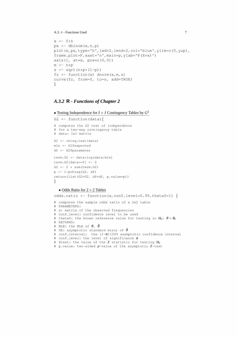
x <- 0:npx <- dbinom(x,n,p)plot(x,px,type="h",lwd=2,lend=2,col="blue",ylim=c(0 ,yup),frame.plot=F,xaxt="n",main=p,ylab="P(X=x)")axis(1, at=x, pos=c(0,0))m <- n* ps <- sqrt(n * p* (1-p))fz <- function(x) dnorm(x,m,s)curve(fz, from=0, to=n, add=TRUE)}
A.3.2 R - Functions of Chapter 2
• Testing Independence forI × J Contingency Tables byG2
G2 <- function(data) {
# computes the G2 test of independence# for a two-way contingency table# data: IxJ matrix
X2 <- chisq.test(data)
mle <- X2$expected
df <- X2$parameter
term.G2 <- data * log(data/mle)
term.G2[data==0] <- 0
G2 <- 2 * sum(term.G2)
p <- 1-pchisq(G2, df)
return(list(G2=G2, df=df, p.value=p))
}
• Odds Ratio for 2×2 Tables
odds.ratio <- function(x,conf.level=0.95,theta0=1) {
# computes the sample odds ratio of a 2x2 table# PARAMETERS:# x: matrix of the observed frequencies# conf.level: confidence level to be used# theta0: the known reference value for testing in H0: θ = θ0# RETURNS:# MLE: the MLE of θ , θ# SE: asymptotic standard error of θ# conf.interval: the (1- α)100% asymptotic confidence interval# conf.level: the level of significance α# Ztest: the value of the Z statistic for testing H0# p.value: two-sided p-value of the asymptotic Z-test
8 A. Web Appendix: Contingency Table Analysis in Practice
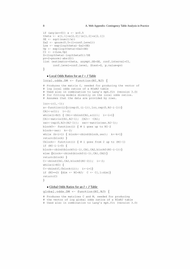
if (any(x==0)) x <- x+0.5theta <- x[1,1] * x[2,2]/(x[1,2] * x[2,1])SE <- sqrt(sum(1/x))Za2 <- qnorm(0.5 * (1+conf.level))Low <- exp(log(theta)-Za2 * SE)Up <- exp(log(theta)+Za2 * SE)CI <- c(Low,Up)Z=(log(theta)-log(theta0))/SEpv=2 * pnorm(-abs(Z))list (estimator=theta, asympt.SE=SE, conf.interval=CI,
conf.level=conf.level, Ztest=Z, p.value=pv)
}
• Local Odds Ratios for anI × J Table
local.odds.DM <- function(NI,NJ) {
# Produces the matrix C, needed for producing the vector of# log local odds ratios of a NIxNJ table# Used also in combination to Lang’s mph.fit (version 3.0)# for fitting models directly on the local odds ratios.# Assumes that the data are provided by rows.
loc<-c(1,-1);
a<-function(i) {c(rep(0,(i-1)),loc,rep(0,NJ-i-1)) }
CA1<-a(1); i<-2;
while(i<NJ) { CA1<-rbind(CA1,a(i)); i<-i+1 }
CA1<-matrix(CA1,NJ-1); CA2<- -CA1;
zer<-rep(0,NJ * (NJ-1)); zer<-matrix(zer,NJ-1);
block0<- function(i) { # i goes up to NI-2
block<-zer; k<-2;
while (k<i+1) { block<-cbind(block,zer); k<-k+1 }
return(block) }
Cblock<- function(i) { # i goes from 2 up to (NI-1)
if (NI-i-1>0) {
block<-cbind(block0(i-1),CA1,CA2,block0(NI-i-1)) }
else {block<-cbind(block0(i-1),CA1,CA2) }
return(block) }
C<-cbind(CA1,CA2,block0(NI-2)); i<-2;
while(i<NI) {
C<-rbind(C,Cblock(i)); i<-i+1 }
if (NI==2) {dim <- NI * NJ; C <- C[,1:dim] }
return(C)
}
• Global Odds Ratios for anI × J Table
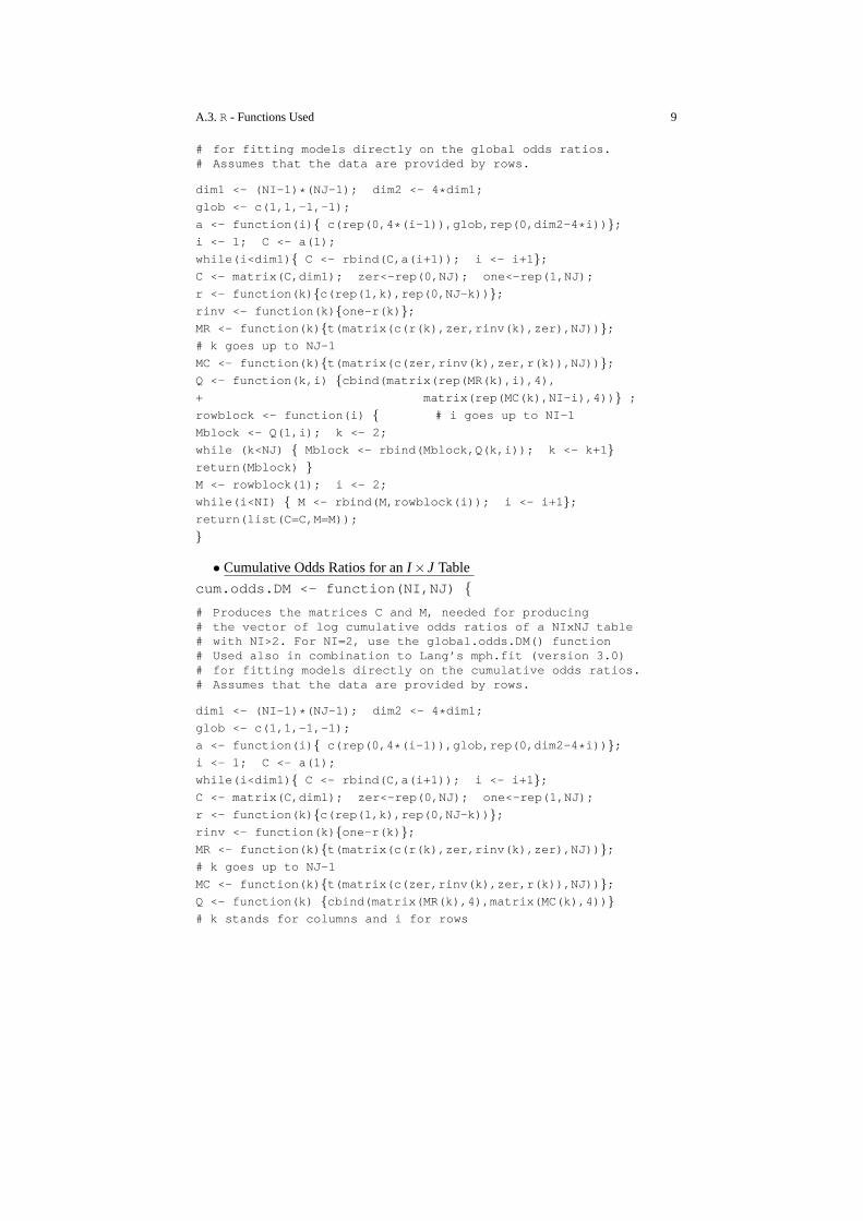
global.odds.DM <- function(NI,NJ) {
# Produces the matrices C and M, needed for producing# the vector of log global odds ratios of a NIxNJ table# Used also in combination to Lang’s mph.fit (version 3.0)
A.3. R - Functions Used 9
# for fitting models directly on the global odds ratios.# Assumes that the data are provided by rows.
dim1 <- (NI-1) * (NJ-1); dim2 <- 4 * dim1;
glob <- c(1,1,-1,-1);
a <- function(i) { c(rep(0,4 * (i-1)),glob,rep(0,dim2-4 * i)) };
i <- 1; C <- a(1);
while(i<dim1) { C <- rbind(C,a(i+1)); i <- i+1 };
C <- matrix(C,dim1); zer<-rep(0,NJ); one<-rep(1,NJ);
r <- function(k) {c(rep(1,k),rep(0,NJ-k)) };
rinv <- function(k) {one-r(k) };
MR <- function(k) {t(matrix(c(r(k),zer,rinv(k),zer),NJ)) };
# k goes up to NJ-1
MC <- function(k) {t(matrix(c(zer,rinv(k),zer,r(k)),NJ)) };
Q <- function(k,i) {cbind(matrix(rep(MR(k),i),4),
+ matrix(rep(MC(k),NI-i),4)) } ;
rowblock <- function(i) { # i goes up to NI-1
Mblock <- Q(1,i); k <- 2;
while (k<NJ) { Mblock <- rbind(Mblock,Q(k,i)); k <- k+1 }
return(Mblock) }
M <- rowblock(1); i <- 2;
while(i<NI) { M <- rbind(M,rowblock(i)); i <- i+1 };
return(list(C=C,M=M));
}
• Cumulative Odds Ratios for anI × J Table
cum.odds.DM <- function(NI,NJ) {
# Produces the matrices C and M, needed for producing# the vector of log cumulative odds ratios of a NIxNJ table# with NI>2. For NI=2, use the global.odds.DM() function# Used also in combination to Lang’s mph.fit (version 3.0)# for fitting models directly on the cumulative odds ratios.# Assumes that the data are provided by rows.
dim1 <- (NI-1) * (NJ-1); dim2 <- 4 * dim1;
glob <- c(1,1,-1,-1);
a <- function(i) { c(rep(0,4 * (i-1)),glob,rep(0,dim2-4 * i)) };
i <- 1; C <- a(1);
while(i<dim1) { C <- rbind(C,a(i+1)); i <- i+1 };
C <- matrix(C,dim1); zer<-rep(0,NJ); one<-rep(1,NJ);
r <- function(k) {c(rep(1,k),rep(0,NJ-k)) };
rinv <- function(k) {one-r(k) };
MR <- function(k) {t(matrix(c(r(k),zer,rinv(k),zer),NJ)) };
# k goes up to NJ-1
MC <- function(k) {t(matrix(c(zer,rinv(k),zer,r(k)),NJ)) };
Q <- function(k) {cbind(matrix(MR(k),4),matrix(MC(k),4)) }
# k stands for columns and i for rows

10 A. Web Appendix: Contingency Table Analysis in Practice
Qblock <- Q(1); k <- 2;
while (k<NJ) { Qblock <- rbind(Qblock,Q(k)); k<- k+1 }
Mzer <- Qblock[,1:NJ]-Qblock[,1:NJ]
ZZ <- function(i) { W<-Mzer; k<-1;
if (i>1) {while (k<i) {W<- cbind(W,Mzer); k<-k+1 } }
return(W) }
rowblock <- function(i) {W2 <- cbind(ZZ(i-1), Qblock, ZZ(NI-i-1));
return(W2) }
Mf <- cbind(ZZ(NI-2),Qblock);
M <- cbind(Qblock,ZZ(NI-2)); i<-2;
while(i<NI-1) { M<-rbind(M,rowblock(i)); i<-i+1 };
M <- rbind(M,Mf);
return(list(C=C,M=M));
}
• Continuation Odds Ratios for anI × J Table
cont.odds.DM <- function(NI,NJ,iflag) {
# Produces the matrices C and M, needed for producing# the vector of log continuation odds ratios of a NIxNJ table# continuation odds ratios of type 1 --> iflag=1# continuation odds ratios of type 2 --> iflag=2# Can also be used for fitting models directly on the# continuation odds ratios.# Assumes that the data are provided by rows.
dim1 <- (NI-1) * (NJ-1); dim2 <- 4 * dim1;
glob <- c(1,1,-1,-1);
a <- function(i) { c(rep(0,4 * (i-1)),glob,rep(0,dim2-4 * i)) };
i <- 1; C <- a(1);
while(i<dim1) { C <- rbind(C,a(i+1)); i <- i+1 };
C <- matrix(C,dim1); zer<-rep(0,NJ); one<-rep(1,NJ);
r <- function(k) {c(rep(1,k),rep(0,NJ-k)) };
rinv <- function(k) {one-r(k) };
r c<-function(k) {r(k)-r(k-1) }
# consider only the specific cell and not the sum up to this
MRc<-function(k) {t(matrix(c(r c(k),zer,rinv(k),zer),NJ)) };
# k goes up to NJ-1
MCc<-function(k) {t(matrix(c(zer,rinv(k),zer,r c(k)),NJ)) };
MR0<-function(k) {t(matrix(c(MR c(k)[1,],zer,MR c(k)[3,],zer),NJ)) };
MRc1<-function(k) {MRc(k)-MR 0(k) };
if (iflag==1) { Mzer <- matrix(rep(zer,4),4);
Q c <- function(k,i) {cbind(matrix(rep(MR c1(k),i-1),4), MR c(k),
+ MCc(k), matrix(rep(Mzer,NI-i-1),4)) }}
else {Q c <- function(k,i) {cbind(matrix(rep(MR c1(k),i-1),4),
+ MRc(k), matrix(rep(MC c(k),NI-i),4)) }}
rowblock<- function(i) { # i goes up to NI-1
Mblock <- Q c(1,i); k <- 2;
A.3. R - Functions Used 11
while (k<NJ) { Mblock <- rbind(Mblock,Q c(k,i)); k <- k+1; }
return(Mblock) }
M <- rowblock(1); i <- 2;
while(i<NI) { M<-rbind(M,rowblock(i)); i<-i+1 }
return(list(C=C,M=M))
}
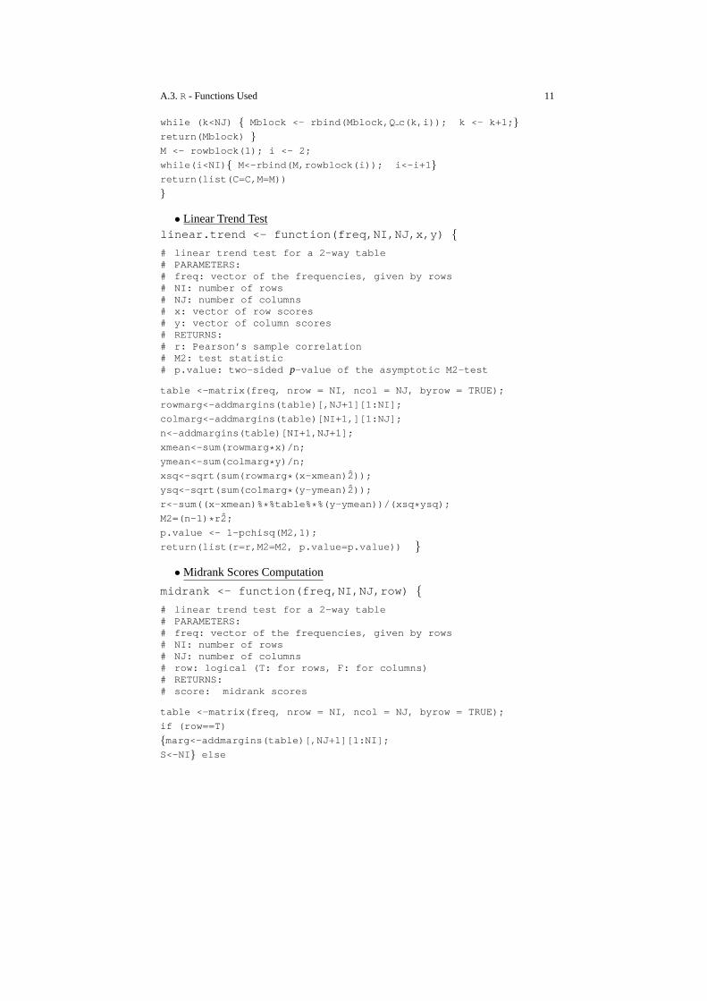
• Linear Trend Testlinear.trend <- function(freq,NI,NJ,x,y) {
# linear trend test for a 2-way table# PARAMETERS:# freq: vector of the frequencies, given by rows# NI: number of rows# NJ: number of columns# x: vector of row scores# y: vector of column scores# RETURNS:# r: Pearson’s sample correlation# M2: test statistic# p.value: two-sided p-value of the asymptotic M2-test
table <-matrix(freq, nrow = NI, ncol = NJ, byrow = TRUE);
rowmarg<-addmargins(table)[,NJ+1][1:NI];
colmarg<-addmargins(table)[NI+1,][1:NJ];
n<-addmargins(table)[NI+1,NJ+1];
xmean<-sum(rowmarg * x)/n;
ymean<-sum(colmarg * y)/n;
xsq<-sqrt(sum(rowmarg * (x-xmean) 2));
ysq<-sqrt(sum(colmarg * (y-ymean) 2));
r<-sum((x-xmean)% * %table% * %(y-ymean))/(xsq * ysq);
M2=(n-1) * r 2;
p.value <- 1-pchisq(M2,1);
return(list(r=r,M2=M2, p.value=p.value)) }
• Midrank Scores Computation
midrank <- function(freq,NI,NJ,row) {
# linear trend test for a 2-way table# PARAMETERS:# freq: vector of the frequencies, given by rows# NI: number of rows# NJ: number of columns# row: logical (T: for rows, F: for columns)# RETURNS:# score: midrank scores
table <-matrix(freq, nrow = NI, ncol = NJ, byrow = TRUE);
if (row==T)
{marg<-addmargins(table)[,NJ+1][1:NI];
S<-NI } else

12 A. Web Appendix: Contingency Table Analysis in Practice
{marg<-addmargins(table)[NI+1,][1:NJ];
S<-NJ }
dd<-c(1,cumsum(marg)+1)
sc1<-1:S
for ( k in (1:S) )
{sc1[k]<-sum(dd[1:S][k]:cumsum(marg)[k]) }
score<-sc1/marg
return(score) }
• Fourfold Plots for the Local Odds Ratios of an IxJ Tableffold.local <- function(x) {
# produces the fourfold plots of the local odds ratios# of an IxJ table in an (I-1)x(J-1) matrix form# PARAMETERS:# x: the data in matrix form
I <- dim(x)[1]; J <- dim(x)[2]
I1 <- I-1; J1 <- J-1
par(mfrow=c(I1,J1))
# par(oma = c(21,0,0,0)) # used to produce Fig. 2.4,
# to reduce the spacing between the two rows of plots
for (i in 1:I1) {for (j in 1:J1) {
i1 <- i+1; j1 <- j+1
y <- x[i:i1, j:j1]
fourfoldplot(y, color = c("#CCCCCC", "#999999")) }}
}
A.3.3 R - Functions of Chapter 3
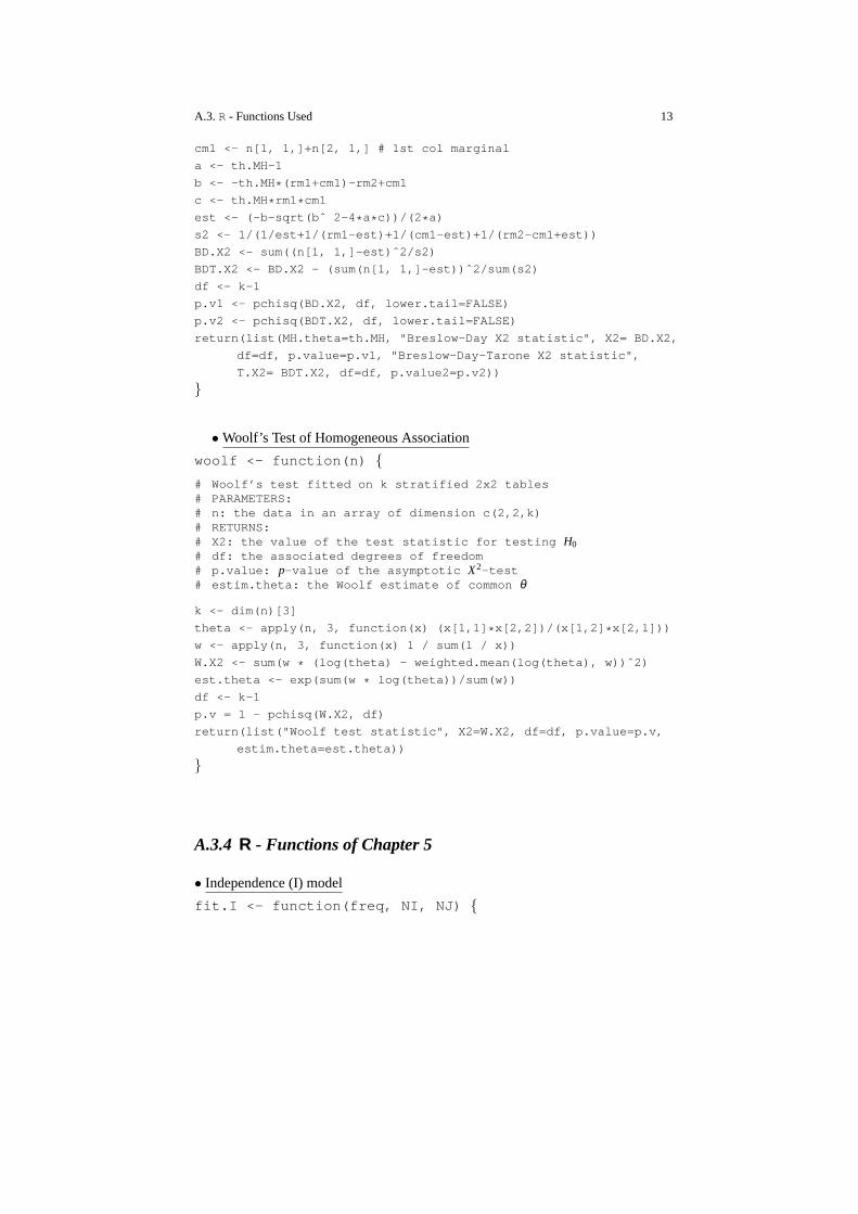
• Breslow-Day-Tarone Test of Homogeneous Association
BDT <- function(n) {
# Breslow-Day test fitted on k stratified 2x2 tables# with and without Tarone’s adjustment# PARAMETERS:# n: the data in an array of dimension c(2,2,k)# RETURNS:# MH.theta: the Mantel Haenszel estimate of common θ# X2: the value of the test statistic for testing H0# df: the associated degrees of freedom# p.value: p-value of the asymptotic X2-test
k <- dim(n)[3]
n.k <- apply(n, 3, sum)
th.MH <- mantelhaen.test(n)$estimate
rm1 <- n[1, 1,]+n[1, 2,] # 1st row marginal
rm2 <- n[2, 1,]+n[2, 2,] # 2d row marginal
A.3. R - Functions Used 13
cm1 <- n[1, 1,]+n[2, 1,] # 1st col marginal
a <- th.MH-1
b <- -th.MH * (rm1+cm1)-rm2+cm1
c <- th.MH * rm1* cm1
est <- (-b-sqrt(bˆ 2-4 * a* c))/(2 * a)
s2 <- 1/(1/est+1/(rm1-est)+1/(cm1-est)+1/(rm2-cm1+est ))
BD.X2 <- sum((n[1, 1,]-est)ˆ2/s2)
BDT.X2 <- BD.X2 - (sum(n[1, 1,]-est))ˆ2/sum(s2)
df <- k-1
p.v1 <- pchisq(BD.X2, df, lower.tail=FALSE)
p.v2 <- pchisq(BDT.X2, df, lower.tail=FALSE)
return(list(MH.theta=th.MH, "Breslow-Day X2 statistic" , X2= BD.X2,
. df=df, p.value=p.v1, "Breslow-Day-Tarone X2 statistic",
. T.X2= BDT.X2, df=df, p.value2=p.v2))
}.
• Woolf’s Test of Homogeneous Association
woolf <- function(n) {
# Woolf’s test fitted on k stratified 2x2 tables# PARAMETERS:# n: the data in an array of dimension c(2,2,k)# RETURNS:# X2: the value of the test statistic for testing H0# df: the associated degrees of freedom# p.value: p-value of the asymptotic X2-test# estim.theta: the Woolf estimate of common θ
k <- dim(n)[3]
theta <- apply(n, 3, function(x) (x[1,1] * x[2,2])/(x[1,2] * x[2,1]))
w <- apply(n, 3, function(x) 1 / sum(1 / x))
W.X2 <- sum(w * (log(theta) - weighted.mean(log(theta), w))ˆ2)
est.theta <- exp(sum(w * log(theta))/sum(w))
df <- k-1
p.v = 1 - pchisq(W.X2, df)
return(list("Woolf test statistic", X2=W.X2, df=df, p.va lue=p.v,
. estim.theta=est.theta))
}
A.3.4 R - Functions of Chapter 5
• Independence (I) model
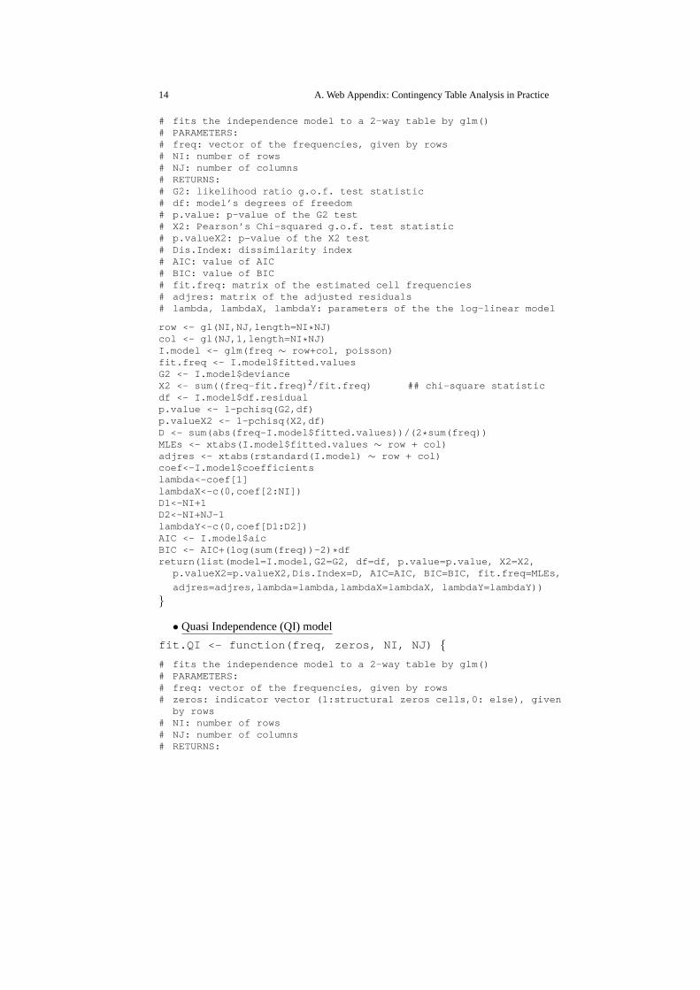
fit.I <- function(freq, NI, NJ) {
14 A. Web Appendix: Contingency Table Analysis in Practice
# fits the independence model to a 2-way table by glm()# PARAMETERS:# freq: vector of the frequencies, given by rows# NI: number of rows# NJ: number of columns# RETURNS:# G2: likelihood ratio g.o.f. test statistic# df: model’s degrees of freedom# p.value: p-value of the G2 test# X2: Pearson’s Chi-squared g.o.f. test statistic# p.valueX2: p-value of the X2 test# Dis.Index: dissimilarity index# AIC: value of AIC# BIC: value of BIC# fit.freq: matrix of the estimated cell frequencies# adjres: matrix of the adjusted residuals# lambda, lambdaX, lambdaY: parameters of the the log-linea r model
row <- gl(NI,NJ,length=NI * NJ)col <- gl(NJ,1,length=NI * NJ)I.model <- glm(freq ∼ row+col, poisson)fit.freq <- I.model$fitted.valuesG2 <- I.model$devianceX2 <- sum((freq-fit.freq) 2/fit.freq) ## chi-square statisticdf <- I.model$df.residualp.value <- 1-pchisq(G2,df)p.valueX2 <- 1-pchisq(X2,df)D <- sum(abs(freq-I.model$fitted.values))/(2 * sum(freq))MLEs <- xtabs(I.model$fitted.values ∼ row + col)adjres <- xtabs(rstandard(I.model) ∼ row + col)coef<-I.model$coefficientslambda<-coef[1]lambdaX<-c(0,coef[2:NI])D1<-NI+1D2<-NI+NJ-1lambdaY<-c(0,coef[D1:D2])AIC <- I.model$aicBIC <- AIC+(log(sum(freq))-2) * dfreturn(list(model=I.model,G2=G2, df=df, p.value=p.val ue, X2=X2,
p.valueX2=p.valueX2,Dis.Index=D, AIC=AIC, BIC=BIC, fit .freq=MLEs,
adjres=adjres,lambda=lambda,lambdaX=lambdaX, lambdaY =lambdaY))
}
• Quasi Independence (QI) model
fit.QI <- function(freq, zeros, NI, NJ) {
# fits the independence model to a 2-way table by glm()# PARAMETERS:# freq: vector of the frequencies, given by rows# zeros: indicator vector (1:structural zeros cells,0: els e), given
by rows# NI: number of rows# NJ: number of columns# RETURNS:

A.3. R - Functions Used 15
# G2: likelihood ratio g.o.f. test statistic# X2: Pearson’s Chi-squared g.o.f. test statistic# df: model’s degrees of freedom# fit.freq: the estimated cell frequencies, given by rows# adjres: the adjusted residuals, given by rows# p.value: p-value of the G2 test# p.valueX2: p-value of the X2 test# lambda, lambdaX, lambdaY: parameters of the the log-linea r model
row <- gl(NI,NJ,length=NI * NJ)col <- gl(NJ,1,length=NI * NJ)example <- data.frame(row, col, freq, zeros)example2 <-example[example$zeros==0,]QI.model <- glm(freq ∼ row+col, data=example2, family=poisson())G2 <- QI.model$deviancedf <- QI.model$df.residualovw <- summary(QI.model)adjres <- xtabs(rstandard(QI.model) ∼ row + col, data = example2)cell.MLE <- xtabs(QI.model$fitted.values ∼ row + col, data = example2)fit.freq <- QI.model$fitted.valuesfreq2<-example2$freqX2<-sum(((freq2-fit.freq) 2)/fit.freq) ## chi-square statisticp.value <- 1-pchisq(G2,df)p.valueX2 <- 1-pchisq(X2,df)coef<-QI.model$coefficientslambda<-coef[1]lambdaX<-c(0,coef[2:NI])D1<-NI+1D2<-NI+NJ-1lambdaY<-c(0,coef[D1:D2])return(list(model=QI.model, G2=G2, df=df, p.value=p.va lue, X2=X2,
p.valueX2=p.valueX2, overview=ovw, fit.freq=cell.MLE,
adjres=adjres, lambda=lambda,lambdaX=lambdaX, lambdaY =lambdaY))
}
A.3.5 R - Functions of Chapter 6
• Scores’ rescaling to obey the weighted constraints (6.17)
rescale <- function(score, dtable, iflag, rows) {
# rescales the vector of scores ’score’ to obbay the# sum-to-0 and sum of squares-to-1 constraints with# marginal (iflag=1) or uniform (iflag=0) weights# called by the functions fitting the association models# PARAMETERS:# score: vector of scores# dtable: data frame of data with the variables freq, X, Y# iflag: flag for selecting marginal (=1) or uniform (=0) wei ghts# rows: for row scores =1 <-> for column scores =0# RETURNS:
16 A. Web Appendix: Contingency Table Analysis in Practice
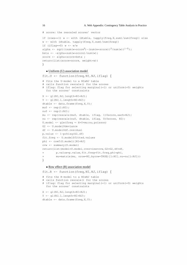
# score: the rescaled scores’ vector
if (rows==1) w <- with (dtable, tapply(freq,X,sum)/sum(fr eq)) else
w <- with (dtable, tapply(freq,Y,sum)/sum(freq))
if (iflag==0) w <- w/w
alpha <- sqrt((sum(w * score 2)-(sum(w * score)) 2/sum(w)) (−1));
beta <- -alpha * sum(w* score)/sum(w);
score <- alpha * score+beta ;
return(list(score=score, weight=w))
}
• Uniform (U) association model
fit.U <- function(freq,NI,NJ,iflag) {
# fits the U-model to a NIxNJ table# calls function rescale() for the scores# iflag: flag for selecting marginal(=1) or uniform(=0) wei ghts
for the scores’ constraints
X <- gl(NI,NJ,length=NI * NJ);
Y <- gl(NJ,1,length=NI * NJ);
dtable <- data.frame(freq,X,Y);
mu0 <- rep(1:NI);
nu0 <- rep(1:NJ);
mu <- rep(rescale(mu0, dtable, iflag, 1)$score,each=NJ);
nu <- rep(rescale(nu0, dtable, iflag, 0)$score, NI);
U.model <- glm(freq ∼ X+Y+mu:nu,poisson)
G2 <- U.model$deviance
df <- U.model$df.residual
p.value <- 1-pchisq(G2,df)
fit.freq <- U.model$fitted.values
phi <- coef(U.model)[NI+NJ]
ovw <- summary(U.model)
return(list(model=U.model,overview=ovw,G2=G2,df=df,
+ p.value=p.value,fit.freq=fit.freq,phi=phi,
+ mu=matrix(mu, nrow=NI,byrow=TRUE)[1:NI],nu=nu[1:NJ] ))
}
• Row effect (R) association model
fit.R <- function(freq,NI,NJ,iflag) {
# fits the R-model to a NIxNJ table# calls function rescale() for the scores# iflag: flag for selecting marginal(=1) or uniform(=0) wei ghts
for the scores’ constraints
X <- gl(NI,NJ,length=NI * NJ);
Y <- gl(NJ,1,length=NI * NJ);
dtable <- data.frame(freq,X,Y);
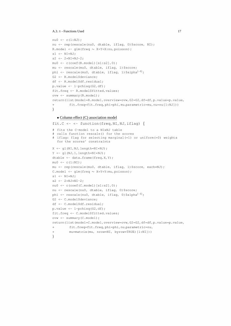
A.3. R - Functions Used 17
nu0 <- c(1:NJ);
nu <- rep(rescale(nu0, dtable, iflag, 0)$score, NI);
R.model <- glm(freq ∼ X+Y+X:nu,poisson);
s1 <- NI+NJ;
s2 <- 2 * NI+NJ-2;
mu0 <- c(coef(R.model)[s1:s2],0);
mu <- rescale(mu0, dtable, iflag, 1)$score;
phi <- rescale(mu0, dtable, iflag, 1)$alpha (−1);
G2 <- R.model$deviance;
df <- R.model$df.residual;
p.value <- 1-pchisq(G2,df);
fit.freq <- R.model$fitted.values;
ovw <- summary(R.model);
return(list(model=R.model,overview=ovw,G2=G2,df=df, p.value=p.value,
+ fit.freq=fit.freq,phi=phi,mu parametric=mu,nu=nu[1:NJ]))
}
• Column effect (C) association model
fit.C <- <- function(freq,NI,NJ,iflag) {
# fits the C-model to a NIxNJ table# calls function rescale() for the scores# iflag: flag for selecting marginal(=1) or uniform(=0) wei ghts
for the scores’ constraints
X <- gl(NI,NJ,length=NI * NJ);
Y <- gl(NJ,1,length=NI * NJ);
dtable <- data.frame(freq,X,Y);
mu0 <- c(1:NI);
mu <- rep(rescale(mu0, dtable, iflag, 1)$score, each=NJ);
C.model <- glm(freq ∼ X+Y+Y:mu,poisson);
s1 <- NI+NJ;
s2 <- 2 * NJ+NI-2;
nu0 <- c(coef(C.model)[s1:s2],0);
nu <- rescale(nu0, dtable, iflag, 0)$score;
phi <- rescale(nu0, dtable, iflag, 0)$alpha (−1);
G2 <- C.model$deviance;
df <- C.model$df.residual;
p.value <- 1-pchisq(G2,df);
fit.freq <- C.model$fitted.values;
ovw <- summary(C.model);
return(list(model=C.model,overview=ovw,G2=G2,df=df, p.value=p.value,
+ fit.freq=fit.freq,phi=phi,nu parametric=nu,
+ mu=matrix(mu, nrow=NI, byrow=TRUE)[1:NI]))
}
18 A. Web Appendix: Contingency Table Analysis in Practice
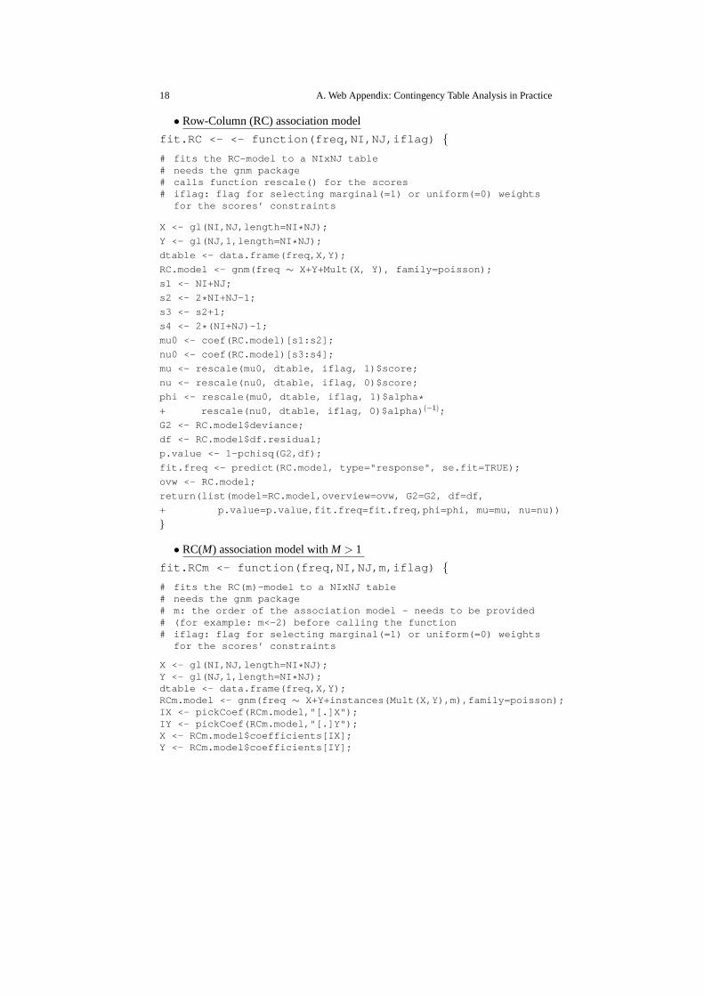
• Row-Column (RC) association model
fit.RC <- <- function(freq,NI,NJ,iflag) {
# fits the RC-model to a NIxNJ table# needs the gnm package# calls function rescale() for the scores# iflag: flag for selecting marginal(=1) or uniform(=0) wei ghts
for the scores’ constraints
X <- gl(NI,NJ,length=NI * NJ);
Y <- gl(NJ,1,length=NI * NJ);
dtable <- data.frame(freq,X,Y);
RC.model <- gnm(freq ∼ X+Y+Mult(X, Y), family=poisson);
s1 <- NI+NJ;
s2 <- 2 * NI+NJ-1;
s3 <- s2+1;
s4 <- 2 * (NI+NJ)-1;
mu0 <- coef(RC.model)[s1:s2];
nu0 <- coef(RC.model)[s3:s4];
mu <- rescale(mu0, dtable, iflag, 1)$score;
nu <- rescale(nu0, dtable, iflag, 0)$score;
phi <- rescale(mu0, dtable, iflag, 1)$alpha *+ rescale(nu0, dtable, iflag, 0)$alpha) (−1);
G2 <- RC.model$deviance;
df <- RC.model$df.residual;
p.value <- 1-pchisq(G2,df);
fit.freq <- predict(RC.model, type="response", se.fit=T RUE);
ovw <- RC.model;
return(list(model=RC.model,overview=ovw, G2=G2, df=df ,
+ p.value=p.value,fit.freq=fit.freq,phi=phi, mu=mu, nu =nu))
}
• RC(M) association model withM > 1
fit.RCm <- function(freq,NI,NJ,m,iflag) {
# fits the RC(m)-model to a NIxNJ table# needs the gnm package# m: the order of the association model - needs to be provided# (for example: m<-2) before calling the function# iflag: flag for selecting marginal(=1) or uniform(=0) wei ghts
for the scores’ constraints
X <- gl(NI,NJ,length=NI * NJ);Y <- gl(NJ,1,length=NI * NJ);dtable <- data.frame(freq,X,Y);RCm.model <- gnm(freq ∼ X+Y+instances(Mult(X,Y),m),family=poisson);IX <- pickCoef(RCm.model,"[.]X");IY <- pickCoef(RCm.model,"[.]Y");X <- RCm.model$coefficients[IX];Y <- RCm.model$coefficients[IY];
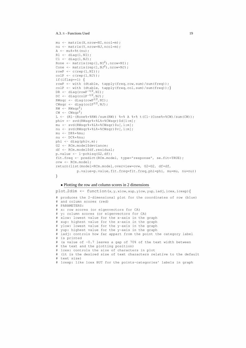
A.3. R - Functions Used 19
mu <- matrix(X,nrow=NI,ncol=m);nu <- matrix(Y,nrow=NJ,ncol=m);A <- mu%* %t(nu);R1 <- diag(1,NI);C1 <- diag(1,NJ);Rone <- matrix(rep(1,NI 2),nrow=NI);Cone <- matrix(rep(1,NJ 2),nrow=NJ);rowP <- c(rep(1,NI));colP <- c(rep(1,NJ));if(iflag==1) {rowP <- with (dtable, tapply(freq,row,sum)/sum(freq));colP <- with (dtable, tapply(freq,col,sum)/sum(freq)); }DR <- diag(rowP −1/2,NI);DC <- diag(colP −1/2,NJ);RWsqr <- diag(rowP 1/2,NI);CWsqr <- diag(colP 1/2,NJ);RW <- RWsqr2;CW <- CWsqr2;L <- (R1-(Rone% * %RW)/sum(RW)) %* % A %* % t(C1-(Cone% * %CW)/sum(CW));phiv <- svd(RWsqr% * %L%* %CWsqr)$d[1:m];mu <- svd(RWsqr% * %L%* %CWsqr)$u[,1:m];nu <- svd(RWsqr% * %L%* %CWsqr)$v[,1:m];mu <- DR%* %mu;nu <- DC%* %nu;phi <- diag(phiv,m);G2 <- RCm.model$deviance;df <- RCm.model$df.residual;p.value <- 1-pchisq(G2,df);fit.freq <- predict(RCm.model, type="response", se.fit= TRUE);ovw <- RCm.model;return(list(model=RCm.model,overview=ovw, G2=G2, df=d f,
p.value=p.value,fit.freq=fit.freq,phi=phi, mu=mu, nu= nu))
}
• Plotting the row and column scores in 2 dimensions
plot 2dim <- function( x,y,xlow,xup,ylow,yup,ladj,lcex,lcexp) {
# produces the 2-dimensional plot for the coordinates of row (blue)# and column scores (red)# PARAMETERS:# x: row scores (or eigenvectors for CA)# y: column scores (or eigenvectors for CA)# xlow: lowest value for the x-axis in the graph# xup: highest value for the x-axis in the graph# ylow: lowest value for the y-axis in the graph# yup: highest value for the y-axis in the graph# ladj: controls how far appart from the point the category la bel# is printed# (a value of -0.7 leaves a gap of 70% of the text width between# the text and the plotting position)# lcex: controls the size of characters in plot# (it is the desired size of text characters relative to the de fault# text size)# lcexp: like lcex BUT for the points-categories’ labels in g raph

20 A. Web Appendix: Contingency Table Analysis in Practice
y0 <- c(0,0);
x0 <- c(0,0);
x1 <- c(-30,30);
y1 <- c(-30,30);
par(cex=lcex,cex.axis=lcex,cex.lab=lcex);
plot(x1,y0,xlab="1st dimension", ylab="2nd dimension",
+ ylim=c(ylow,yup), xlim=c(xlow,xup),type="l",lty=2);
lines(x0,y1,type="l",lty=2);
points(x[,1],x[,2],pch=19,col="blue");
points(y[,1],y[,2],pch=17,col="red");
a <- length(x[,1]);
b <- length(y[,1]);
namesx <- c(1:a);
namesy <- c(1:b);
text(x[,1],x[,2],namesx,adj=ladj,cex=lcexp);
text(y[,1],y[,2],namesy,adj=ladj,cex=lcexp);
}
A.3.6 R - Functions of Chapter 9
• (1−a)100% asymptotic confidence interval for the differenceof correlated proportions
McNemar.CI <- function(x, a) {
# computes the asymptotic Wald (1-a)100% CI for correlated p roportions# PARAMETERS:# x : the 2x2 frequencies table# a : significance level
p <- prop.table(x)
rp1 <- addmargins(p)[1,3]
cp1 <- addmargins(p)[3,1]
SE <- sqrt((rp1 * (1-rp1)+cp1 * (1-cp1)-2 * (p[1,1] * p[2,2]-p[1,2] * p[2,1]))
+ /sum(x))
Za2 <- -qnorm(0.5 * (0.05))
CI <- rp1-cp1+c(-1,1) * Za2* SE
return(CI)
}
• Factors needed to fit symmetry models inglm
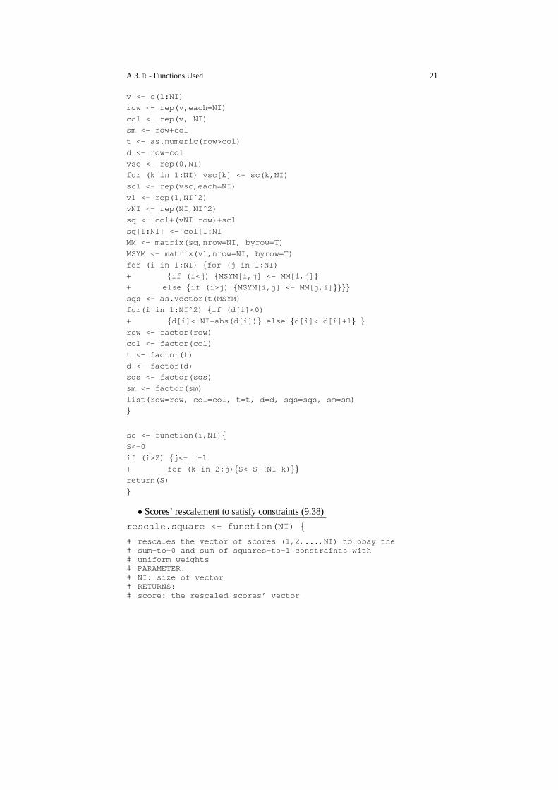
SYMV <-function (NI) {
# produces the factors needed to fit symmetry models in glm# needs function sc()
A.3. R - Functions Used 21
v <- c(1:NI)
row <- rep(v,each=NI)
col <- rep(v, NI)
sm <- row+col
t <- as.numeric(row>col)
d <- row-col
vsc <- rep(0,NI)
for (k in 1:NI) vsc[k] <- sc(k,NI)
sc1 <- rep(vsc,each=NI)
v1 <- rep(1,NIˆ2)
vNI <- rep(NI,NIˆ2)
sq <- col+(vNI-row)+sc1
sq[1:NI] <- col[1:NI]
MM <- matrix(sq,nrow=NI, byrow=T)
MSYM <- matrix(v1,nrow=NI, byrow=T)
for (i in 1:NI) {for (j in 1:NI)
+ {if (i<j) {MSYM[i,j] <- MM[i,j] }
+ else {if (i>j) {MSYM[i,j] <- MM[j,i] }}}}
sqs <- as.vector(t(MSYM)
for(i in 1:NIˆ2) {if (d[i]<0)
+ {d[i]<-NI+abs(d[i]) } else {d[i]<-d[i]+1 } }
row <- factor(row)
col <- factor(col)
t <- factor(t)
d <- factor(d)
sqs <- factor(sqs)
sm <- factor(sm)
list(row=row, col=col, t=t, d=d, sqs=sqs, sm=sm)
}
sc <- function(i,NI) {
S<-0
if (i>2) {j<- i-1
+ for (k in 2:j) {S<-S+(NI-k) }}
return(S)
}
• Scores’ rescalement to satisfy constraints (9.38)
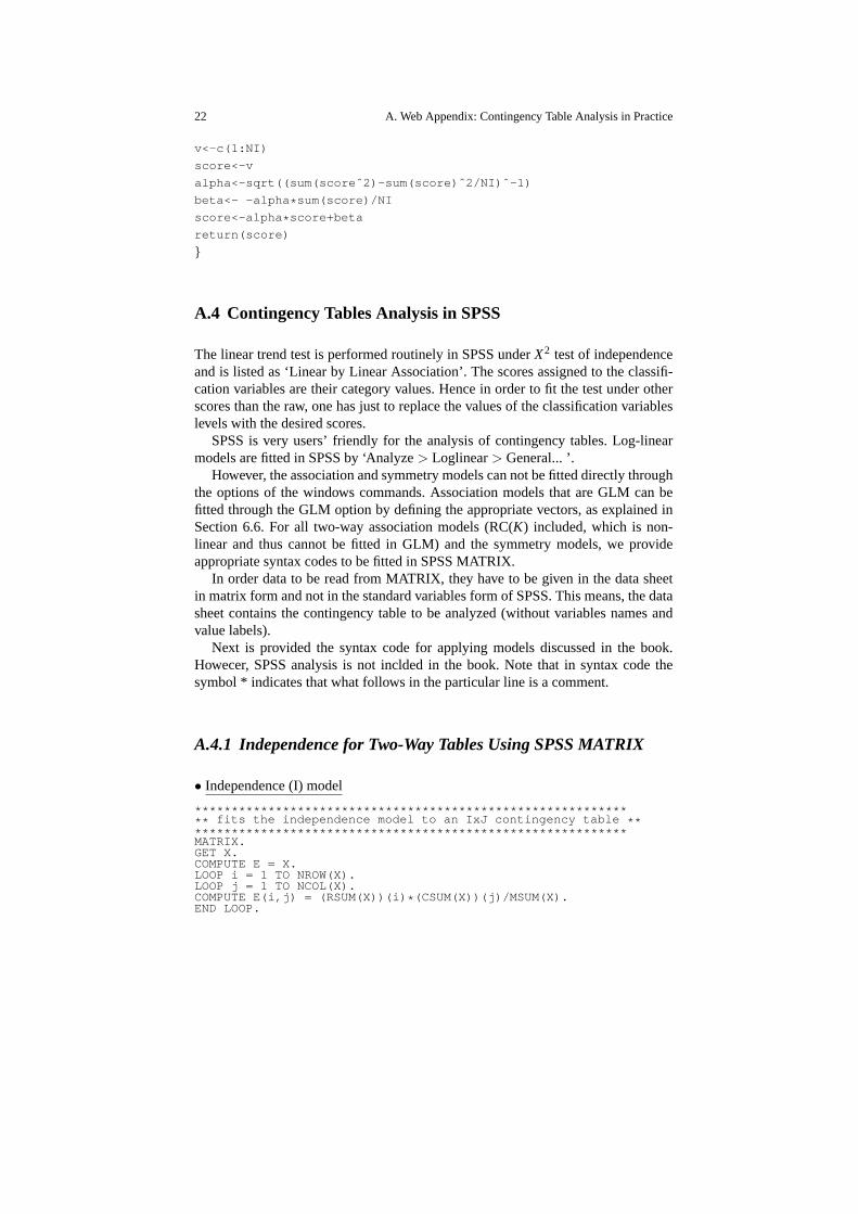
rescale.square <- function(NI) {
# rescales the vector of scores (1,2,...,NI) to obay the# sum-to-0 and sum of squares-to-1 constraints with# uniform weights# PARAMETER:# NI: size of vector# RETURNS:# score: the rescaled scores’ vector
22 A. Web Appendix: Contingency Table Analysis in Practice
v<-c(1:NI)
score<-v
alpha<-sqrt((sum(scoreˆ2)-sum(score)ˆ2/NI)ˆ-1)
beta<- -alpha * sum(score)/NI
score<-alpha * score+beta
return(score)
}
A.4 Contingency Tables Analysis in SPSS
The linear trend test is performed routinely in SPSS underX2 test of independenceand is listed as ‘Linear by Linear Association’. The scores assigned to the classifi-cation variables are their category values. Hence in order to fit the test under otherscores than the raw, one has just to replace the values of the classification variableslevels with the desired scores.
SPSS is very users’ friendly for the analysis of contingencytables. Log-linearmodels are fitted in SPSS by ‘Analyze> Loglinear> General... ’.
However, the association and symmetry models can not be fitted directly throughthe options of the windows commands. Association models that are GLM can befitted through the GLM option by defining the appropriate vectors, as explained inSection 6.6. For all two-way association models (RC(K) included, which is non-linear and thus cannot be fitted in GLM) and the symmetry models, we provideappropriate syntax codes to be fitted in SPSS MATRIX.
In order data to be read from MATRIX, they have to be given in the data sheetin matrix form and not in the standard variables form of SPSS.This means, the datasheet contains the contingency table to be analyzed (without variables names andvalue labels).
Next is provided the syntax code for applying models discussed in the book.Howecer, SPSS analysis is not inclded in the book. Note that in syntax code thesymbol * indicates that what follows in the particular line is a comment.
A.4.1 Independence for Two-Way Tables Using SPSS MATRIX
• Independence (I) model
*************************************************** ********** fits the independence model to an IxJ contingency table ***************************************************** ********MATRIX.GET X.COMPUTE E = X.LOOP i = 1 TO NROW(X).LOOP j = 1 TO NCOL(X).COMPUTE E(i,j) = (RSUM(X))(i) * (CSUM(X))(j)/MSUM(X).END LOOP.

A.4. Contingency Tables Analysis in SPSS 23
END LOOP.PRINT X.PRINT E /FORMAT F10.3.COMPUTE G2 = 2* MSUM( X &* LN(X &/ E) ).COMPUTE X2 = MSUM((X-E)&** 2 &/ E).COMPUTE DF = (NROW(X)-1)* (NCOL(X)-1).COMPUTE SIG = 1 - CHICDF(G2,DF).PRINT G2,DF,SIG /TITLE = "LIKELIHOOD RATIO TEST" /FORMAT F1 0.4 /CLABELS ’G2’,’DF’,’SIG.’.COMPUTE SIG = 1 - CHICDF(X2,DF).PRINT X2,DF,SIG /TITLE = "PEARSON’S X2" /FORMAT F10.4 /CLABELS ’X2’,’DF’,’SIG.’.END MATRIX.
A.4.2 Association Models for Two-Way Tables in SPSS
In SPSS association models can be fitted from the main menu, through‘Analyze> Log Linear> General...’
as described in the sequel.First of all, the data have to be in the standard format for fitting classical
log-linear models. Thus, ifrow and col are the usual variables that are cross-classified the contingency table, first we have to add in the data file (from theTransform>Compute Variables. . .) the variablesu = (row) · (col), mu = row andnu = col. Then, we define these vectorsu, mu and nu as ’cell covariates’ in the’General LogLinear Analysis’ window and the models are specified by the follow-ing ‘Terms in model’:
U: row, col, uR: row, col, row∗nuC: row, col, mu∗ col
The LL model can be fitted as the U model with the only difference that variablesrow andcol will now contain the values of the prefixed, not equidistant scores forthe corresponding row and column categories. Note that by the above procedure,the scores are taken equal to the corresponding category index and thus they donot satisfy the constraints (6.5) and (6.6). The models R andC are defined accord-ing to the (6.15) parameterization, without the intrinsic association parameterϕ. Ifwe want the scores to be standardized, then, we have to compute themu andnuvariables by the corresponding linear transformation ofrow andcol while for mo-dels R and C, the estimates of the parametric scores have to berescaled at a finalstage, where the sum of squares add to one constraint adjustment will produce theϕ parameter estimate. Alternatively, one can use the syntax scripts provided below,which fit these models via the Newton’s unidimensional method subject to the gen-eral constraints (6.17) with the option of uniform or marginal weights. Unlikely, thenon-linear RC(K) model,K ≥ 1, can not be fitted directly in SPSS. Also for the fitof this model a syntax code is given next. The SPSS syntax codefor the associationmodels is jointly written with G. Iliopoulos.

24 A. Web Appendix: Contingency Table Analysis in Practice
• Uniform (U) association model
*************************************************** ********** U model for an IxJ contingency table ***************************************************** ********SET MXLOOP = 20000.MATRIX.GET X.*************************************************** MAR: specifies the weights to be used (1:marginal - 0:unifor m)**************************************************COMPUTE MAR = 0.COMPUTE TOLER = 10** (-15).COMPUTE P = X/MSUM(X).COMPUTE A = RSUM(P).COMPUTE ADIAG = MDIAG(A).COMPUTE B = CSUM(P).COMPUTE BDIAG = MDIAG(B).COMPUTE RI=IDENT(NROW(X)).COMPUTE CI=IDENT(NCOL(X)).COMPUTE RONE=MAKE(NROW(X),NROW(X),1).COMPUTE CONE=MAKE(NCOL(X),NCOL(X),1).COMPUTE RWT=MAKE(NROW(X),NROW(X),0).COMPUTE CWT=MAKE(NCOL(X),NCOL(X),0).DO IF (MAR=1).LOOP I=1 TO NROW(X).COMPUTE RWT(I,I)=RSUM(X)(I)/MSUM(X).END LOOP.LOOP J=1 TO NCOL(X).COMPUTE CWT(J,J)=CSUM(X)(J)/MSUM(X).END LOOP.ELSE.COMPUTE RWT=RI.COMPUTE CWT=CI.END IF.COMPUTE M = MAKE(NROW(X),1,0).LOOP i=1 TO NROW(X).COMPUTE M(i)=i.END LOOP.COMPUTE M=M-RONE* RWT* M/TRACE(RWT).COMPUTE M=M/SQRT(T(M)* RWT* M).COMPUTE N = MAKE(NCOL(X),1,0).LOOP i=1 TO NCOL(X).COMPUTE N(i)=i.END LOOP.COMPUTE N=N-CONE* CWT* N/TRACE(CWT).COMPUTE N=N/SQRT(T(N)* CWT* N).COMPUTE PHI = T(M)* ADIAG* LN(P) * BDIAG* N.COMPUTE PI = ADIAG* EXP(M* PHI * T(N)) * BDIAG.LOOP L = 1 TO 20000.DO IF ( MSUM(ABS(RSUM(P-PI)))+MSUM(ABS(CSUM(P-PI)))+MSUM(ABS(T(M)* (P-PI) * N))<TOLER).BREAK.END IF.COMPUTE AOLD = A.COMPUTE BOLD = B.COMPUTE PHIOLD = PHI.COMPUTE A = AOLD &* (RSUM(P) &/ RSUM(PI)).COMPUTE ADIAG = MDIAG(A).COMPUTE PI = ADIAG* EXP(M* PHI * T(N)) * BDIAG.COMPUTE B = BOLD &* (CSUM(P) &/ CSUM(PI)).COMPUTE BDIAG = MDIAG(B).COMPUTE PI = ADIAG* EXP(M* PHI * T(N)) * BDIAG.COMPUTE PHI = PHIOLD + DIAG ( ( T(M)* (P-PI) * N ) &/( T(M & ** 2) * PI * (N &** 2) ) ).COMPUTE PI = ADIAG* EXP(M* PHI * T(N)) * BDIAG.END LOOP.PRINT L.COMPUTE E = MSUM(X)* PI.PRINT X.

A.4. Contingency Tables Analysis in SPSS 25
PRINT E /FORMAT F10.3.PRINT PI /FORMAT F10.4.PRINT M.PRINT N.PRINT PHI.PRINT EXP(PHI).COMPUTE G2 = 2* MSUM( X &* LN(X &/ E) ).COMPUTE DF = (NROW(X)-1)* (NCOL(X)-1)-1.COMPUTE SIG = 1 - CHICDF(G2,DF).PRINT G2,DF,SIG /TITLE = "LIKELIHOOD RATIO TEST" /FORMAT F1 0.4 /CLABELS ’G2’,’DF’,’SIG.’.END MATRIX.
• Row effect (R) association model
*************************************************** ********** R model for an IxJ contingency table ***************************************************** ********SET MXLOOP = 20000.MATRIX.GET X.************************************************ MAR: specifies the weights to be used (1:marginal - 0:unifor m)************************************************COMPUTE MAR = 0.COMPUTE TOLER = 10** (-15).COMPUTE P = X/MSUM(X).COMPUTE A = RSUM(P).COMPUTE ADIAG = MDIAG(A).COMPUTE B = CSUM(P).COMPUTE BDIAG = MDIAG(B).COMPUTE RI=IDENT(NROW(X)).COMPUTE CI=IDENT(NCOL(X)).COMPUTE RONE=MAKE(NROW(X),NROW(X),1).COMPUTE CONE=MAKE(NCOL(X),NCOL(X),1).COMPUTE RWT=MAKE(NROW(X),NROW(X),0).COMPUTE CWT=MAKE(NCOL(X),NCOL(X),0).DO IF (MAR=1).LOOP I=1 TO NROW(X).COMPUTE RWT(I,I)=RSUM(X)(I)/MSUM(X).END LOOP.LOOP J=1 TO NCOL(X).COMPUTE CWT(J,J)=CSUM(X)(J)/MSUM(X).END LOOP.ELSE.COMPUTE RWT=RI.COMPUTE CWT=CI.END IF.COMPUTE M = MAKE(NROW(X),1,0).LOOP i=1 TO NROW(X).COMPUTE M(i)=i.END LOOP.COMPUTE M=M-RONE* RWT* M/TRACE(RWT).COMPUTE M=M/SQRT(T(M)* RWT* M).COMPUTE N = MAKE(NCOL(X),1,0).LOOP i=1 TO NCOL(X).COMPUTE N(i)=i.END LOOP.COMPUTE N=N-CONE* CWT* N/TRACE(CWT).COMPUTE N=N/SQRT(T(N)* CWT* N).COMPUTE PHI = T(M)* ADIAG* LN(P) * BDIAG* N.COMPUTE PI = ADIAG* EXP(M* PHI * T(N)) * BDIAG.COMPUTE CHECK=10.LOOP L = 1 TO 20000.DO IF ( CHECK<TOLER).BREAK.END IF.COMPUTE AOLD = A.
26 A. Web Appendix: Contingency Table Analysis in Practice
COMPUTE BOLD = B.COMPUTE MOLD = M.COMPUTE PHIOLD = PHI.COMPUTE A = AOLD &* (RSUM(P) &/ RSUM(PI)).COMPUTE ADIAG = MDIAG(A).COMPUTE PI = ADIAG* EXP(M* PHI * T(N)) * BDIAG.COMPUTE B = BOLD &* (CSUM(P) &/ CSUM(PI)).COMPUTE BDIAG = MDIAG(B).COMPUTE PI = ADIAG* EXP(M* PHI * T(N)) * BDIAG.COMPUTE M = MOLD + ((P-PI)* N) &/ (PI * (N &** 2)) .COMPUTE M=M-RONE* RWT* M/TRACE(RWT).COMPUTE M=M/SQRT(T(M)* RWT* M).COMPUTE PI = ADIAG* EXP(M* PHI * T(N)) * BDIAG.COMPUTE PHI = PHIOLD + DIAG ( ( T(M)* (P-PI) * N ) &/( T(M & ** 2) * PI * (N &** 2) ) ).COMPUTE PI = ADIAG* EXP(M* PHI * T(N)) * BDIAG.COMPUTE CHECK=MSUM(ABS(RSUM(P-PI)))+MSUM(ABS(CSUM(P-PI))).COMPUTE CHECK=CHECK+MSUM(ABS(T(M)* (P-PI) * N))+MSUM(ABS((P-PI) * N)).END LOOP.PRINT L.COMPUTE E = MSUM(X)* PI.PRINT X.PRINT E /FORMAT F10.3.PRINT PI /FORMAT F10.4.PRINT M.PRINT N.PRINT PHI.PRINT EXP(PHI).COMPUTE G2 = 2* MSUM( X &* LN(X &/ E) ).COMPUTE DF = (NROW(X)-1)* (NCOL(X)-2).COMPUTE SIG = 1 - CHICDF(G2,DF).PRINT G2,DF,SIG /TITLE = "LIKELIHOOD RATIO TEST" /FORMAT F1 0.4 /CLABELS ’G2’,’DF’,’SIG.’.END MATRIX.
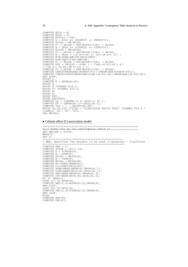
• Column effect (C) association model
*************************************************** ********** C model for an IxJ contingency table ***************************************************** ********SET MXLOOP = 20000.MATRIX.GET X.*************************************************** MAR: specifies the weights to be used (1:marginal - 0:unifor m)***************************************************COMPUTE MAR = 0.COMPUTE TOLER = 10** (-15).COMPUTE P = X/MSUM(X).COMPUTE A = RSUM(P).COMPUTE ADIAG = MDIAG(A).COMPUTE B = CSUM(P).COMPUTE BDIAG = MDIAG(B).COMPUTE RI=IDENT(NROW(X)).COMPUTE CI=IDENT(NCOL(X)).COMPUTE RONE=MAKE(NROW(X),NROW(X),1).COMPUTE CONE=MAKE(NCOL(X),NCOL(X),1).COMPUTE RWT=MAKE(NROW(X),NROW(X),0).COMPUTE CWT=MAKE(NCOL(X),NCOL(X),0).DO IF (MAR=1).LOOP I=1 TO NROW(X).COMPUTE RWT(I,I)=RSUM(X)(I)/MSUM(X).END LOOP.LOOP J=1 TO NCOL(X).COMPUTE CWT(J,J)=CSUM(X)(J)/MSUM(X).END LOOP.ELSE.COMPUTE RWT=RI.COMPUTE CWT=CI.

A.4. Contingency Tables Analysis in SPSS 27
END IF.COMPUTE M = MAKE(NROW(X),1,0).LOOP i=1 TO NROW(X).COMPUTE M(i)=i.END LOOP.COMPUTE M=M-RONE* RWT* M/TRACE(RWT).COMPUTE M=M/SQRT(T(M)* RWT* M).COMPUTE N = MAKE(NCOL(X),1,0).LOOP i=1 TO NCOL(X).COMPUTE N(i)=i.END LOOP.COMPUTE N=N-CONE* CWT* N/TRACE(CWT).COMPUTE N=N/SQRT(T(N)* CWT* N).COMPUTE PHI = T(M)* ADIAG* LN(P) * BDIAG* N.COMPUTE PI = ADIAG* EXP(M* PHI * T(N)) * BDIAG.COMPUTE CHECK=10.LOOP L = 1 TO 20000.DO IF ( CHECK<TOLER).BREAK.END IF.COMPUTE AOLD = A.COMPUTE BOLD = B.COMPUTE NOLD = N.COMPUTE PHIOLD = PHI.COMPUTE A = AOLD &* (RSUM(P) &/ RSUM(PI)).COMPUTE ADIAG = MDIAG(A).COMPUTE PI = ADIAG* EXP(M* PHI * T(N)) * BDIAG.COMPUTE B = BOLD &* (CSUM(P) &/ CSUM(PI)).COMPUTE BDIAG = MDIAG(B).COMPUTE PI = ADIAG* EXP(M* PHI * T(N)) * BDIAG.COMPUTE N = NOLD + (T(P-PI)* M ) &/ (T(PI) * (M &** 2) ).COMPUTE N=N-CONE* CWT* N/TRACE(CWT).COMPUTE N=N/SQRT(T(N)* CWT* N).COMPUTE PI = ADIAG* EXP(M* PHI * T(N)) * BDIAG.COMPUTE PHI = PHIOLD + DIAG ( ( T(M)* (P-PI) * N ) &/( T(M & ** 2) * PI * (N &** 2) ) ).COMPUTE PI = ADIAG* EXP(M* PHI * T(N)) * BDIAG.COMPUTE CHECK=MSUM(ABS(RSUM(P-PI)))+MSUM(ABS(CSUM(P-PI))).COMPUTE CHECK=CHECK+MSUM(ABS(T(M)* (P-PI) * N))+MSUM(ABS(T(M) * (P-PI))).END LOOP.PRINT L.COMPUTE E = MSUM(X)* PI.PRINT X.PRINT E /FORMAT F10.3.PRINT PI /FORMAT F10.4.PRINT M.PRINT N.PRINT PHI.PRINT EXP(PHI).COMPUTE G2 = 2* MSUM( X &* LN(X &/ E) ).COMPUTE DF = (NROW(X)-2)* (NCOL(X)-1).COMPUTE SIG = 1 - CHICDF(G2,DF).PRINT G2,DF,SIG /TITLE = "LIKELIHOOD RATIO TEST" /FORMAT F1 0.4 /CLABELS ’G2’,’DF’,’SIG.’.END MATRIX.
• RC(K) association model
*************************************************** ********** RC(K) model for an IxJ contingency table ***************************************************** ********SET MXLOOP = 20000.MATRIX.GET X.COMPUTE TOLER = 10** (-15).*************************************************** ********* K: number of terms in the sum of the association term.* MAR: specifies the weights to be used (1:marginal - 0:unifor m)

28 A. Web Appendix: Contingency Table Analysis in Practice
*************************************************** ********COMPUTE K = 1.COMPUTE MAR = 0.COMPUTE RI=IDENT(NROW(X)).COMPUTE CI=IDENT(NCOL(X)).COMPUTE RONE=MAKE(NROW(X),NROW(X),1).COMPUTE CONE=MAKE(NCOL(X),NCOL(X),1).COMPUTE RWT=MAKE(NROW(X),NROW(X),0).COMPUTE CWT=MAKE(NCOL(X),NCOL(X),0).DO IF (MAR=1).LOOP I=1 TO NROW(X).COMPUTE RWT(I,I)=RSUM(X)(I)/MSUM(X).END LOOP.LOOP J=1 TO NCOL(X).COMPUTE CWT(J,J)=CSUM(X)(J)/MSUM(X).END LOOP.ELSE.COMPUTE RWT=RI.COMPUTE CWT=CI.END IF.COMPUTE P = X/MSUM(X).LOOP i = 1 TO NROW(X).LOOP j = 1 TO NCOL(X).DO IF (P(i,j)=0).COMPUTE P(i,j)=0.0001.END IF.END LOOP.END LOOP.COMPUTE LOGP=LN(P).*************************************************** ********** L is the matrix of interaction parameters for the model** with weights RWT, CWT .*************************************************** ********COMPUTE L=(RI-RONE* RWT/TRACE(RWT))* LOGP* (CI-CWT * CONE/TRACE(CWT)).PRINT L.CALL SVD(L,U,Q,V).COMPUTE M = U(:,1:K).COMPUTE N = V(:,1:K).COMPUTE PHIDIAG = Q(1:K,1:K).COMPUTE PHI = DIAG(PHIDIAG).COMPUTE A = EXP(RSUM(LOGP))/NCOL(X)-0.5 * MSUM(LOGP)/(NROW(X)* NCOL(X))).COMPUTE ADIAG = MDIAG(A).COMPUTE B = EXP(CSUM(LOGP)/NROW(X)-0.5* MSUM(LOGP)/(NROW(X)* NCOL(X))).COMPUTE BDIAG = MDIAG(B).COMPUTE PI = ADIAG* EXP(M* PHIDIAG* T(N)) * BDIAG.*************************************************** ********COMPUTE CHECK=10.LOOP ITER = 1 TO 20000.DO IF (CHECK<TOLER).BREAK.END IF.COMPUTE AOLD = A.COMPUTE BOLD = B.COMPUTE MOLD = M.COMPUTE NOLD = N.COMPUTE PHIOLD = PHI.** Note 1 : The matrix PI is updated continuously.** Note 2 : After updating M and N, they are multiplied by** appropriate matrices so that the update of M * PHIDIAG* T(N)** satisfies the weights restrictions.COMPUTE A = AOLD &* (RSUM(P) &/ RSUM(PI)).COMPUTE ADIAG = MDIAG(A).COMPUTE PI = ADIAG* EXP(M* PHIDIAG* T(N)) * BDIAG.COMPUTE B = BOLD &* (CSUM(P) &/ CSUM(PI)).COMPUTE BDIAG = MDIAG(B).COMPUTE PI = ADIAG* EXP(M* PHIDIAG* T(N)) * BDIAG.COMPUTE M = MOLD + ((P-PI)* N) &/ (PI * (N &** 2)).COMPUTE M=(RI-RONE* RWT/TRACE(RWT))* M.COMPUTE PI = ADIAG* EXP(M* PHIDIAG* T(N)) * BDIAG.
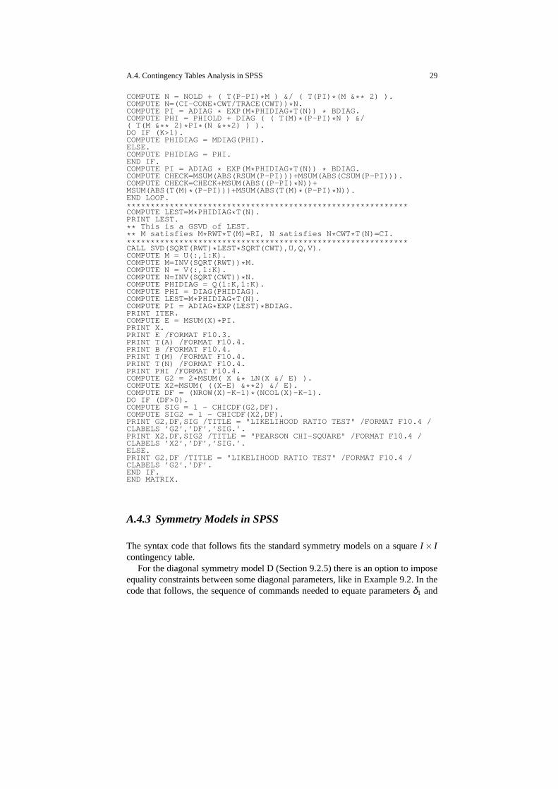
A.4. Contingency Tables Analysis in SPSS 29
COMPUTE N = NOLD + ( T(P-PI)* M ) &/ ( T(PI) * (M &** 2) ).COMPUTE N=(CI-CONE* CWT/TRACE(CWT))* N.COMPUTE PI = ADIAG* EXP(M* PHIDIAG* T(N)) * BDIAG.COMPUTE PHI = PHIOLD + DIAG ( ( T(M)* (P-PI) * N ) &/( T(M & ** 2) * PI * (N &** 2) ) ).DO IF (K>1).COMPUTE PHIDIAG = MDIAG(PHI).ELSE.COMPUTE PHIDIAG = PHI.END IF.COMPUTE PI = ADIAG* EXP(M* PHIDIAG* T(N)) * BDIAG.COMPUTE CHECK=MSUM(ABS(RSUM(P-PI)))+MSUM(ABS(CSUM(P-PI))).COMPUTE CHECK=CHECK+MSUM(ABS((P-PI)* N))+MSUM(ABS(T(M)* (P-PI)))+MSUM(ABS(T(M) * (P-PI) * N)).END LOOP.*************************************************** ********COMPUTE LEST=M* PHIDIAG* T(N).PRINT LEST.** This is a GSVD of LEST.** M satisfies M * RWT* T(M)=RI, N satisfies N * CWT* T(N)=CI.*************************************************** ********CALL SVD(SQRT(RWT)* LEST* SQRT(CWT),U,Q,V).COMPUTE M = U(:,1:K).COMPUTE M=INV(SQRT(RWT))* M.COMPUTE N = V(:,1:K).COMPUTE N=INV(SQRT(CWT))* N.COMPUTE PHIDIAG = Q(1:K,1:K).COMPUTE PHI = DIAG(PHIDIAG).COMPUTE LEST=M* PHIDIAG* T(N).COMPUTE PI = ADIAG* EXP(LEST) * BDIAG.PRINT ITER.COMPUTE E = MSUM(X)* PI.PRINT X.PRINT E /FORMAT F10.3.PRINT T(A) /FORMAT F10.4.PRINT B /FORMAT F10.4.PRINT T(M) /FORMAT F10.4.PRINT T(N) /FORMAT F10.4.PRINT PHI /FORMAT F10.4.COMPUTE G2 = 2* MSUM( X &* LN(X &/ E) ).COMPUTE X2=MSUM( ((X-E) &** 2) &/ E).COMPUTE DF = (NROW(X)-K-1)* (NCOL(X)-K-1).DO IF (DF>0).COMPUTE SIG = 1 - CHICDF(G2,DF).COMPUTE SIG2 = 1 - CHICDF(X2,DF).PRINT G2,DF,SIG /TITLE = "LIKELIHOOD RATIO TEST" /FORMAT F1 0.4 /CLABELS ’G2’,’DF’,’SIG.’.PRINT X2,DF,SIG2 /TITLE = "PEARSON CHI-SQUARE" /FORMAT F10 .4 /CLABELS ’X2’,’DF’,’SIG.’.ELSE.PRINT G2,DF /TITLE = "LIKELIHOOD RATIO TEST" /FORMAT F10.4 /CLABELS ’G2’,’DF’.END IF.END MATRIX.
A.4.3 Symmetry Models in SPSS
The syntax code that follows fits the standard symmetry models on a squareI × Icontingency table.
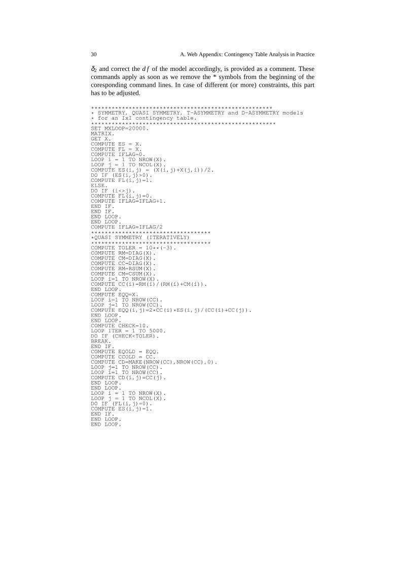
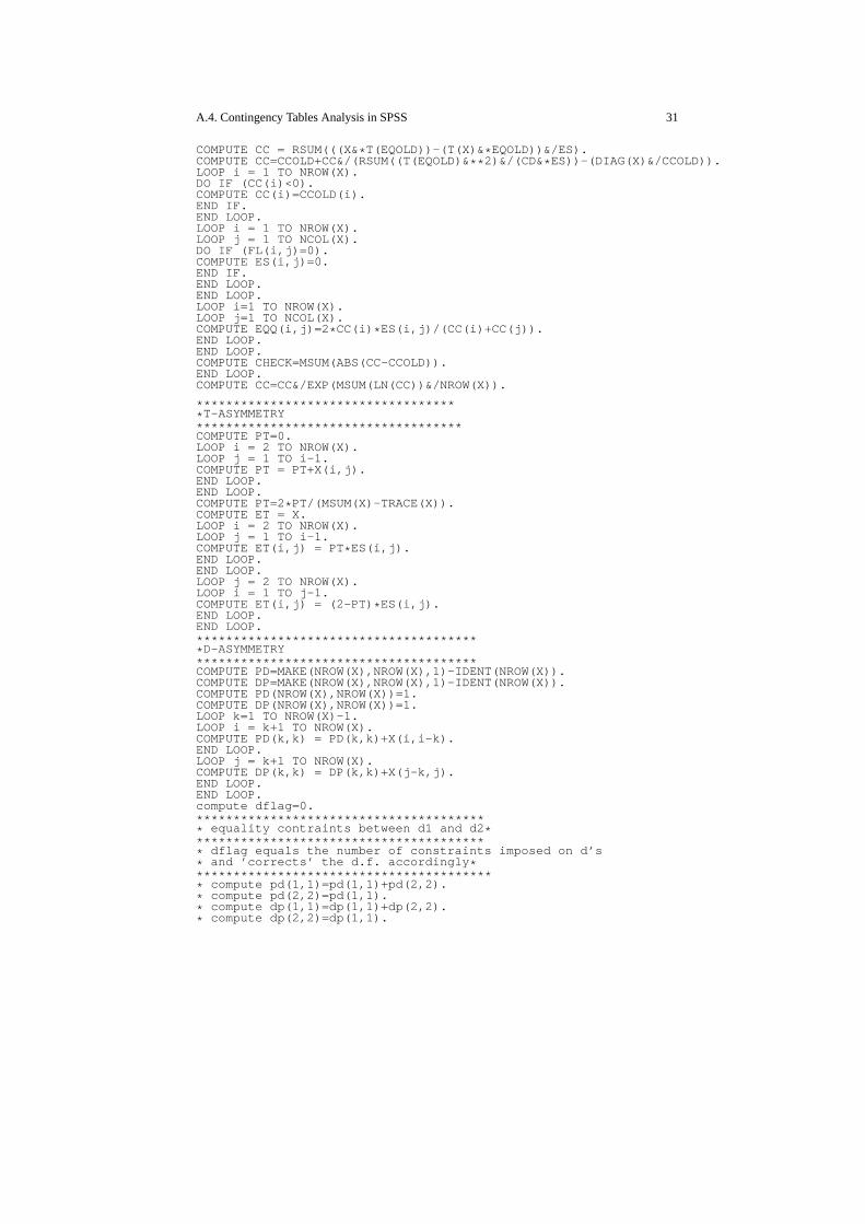
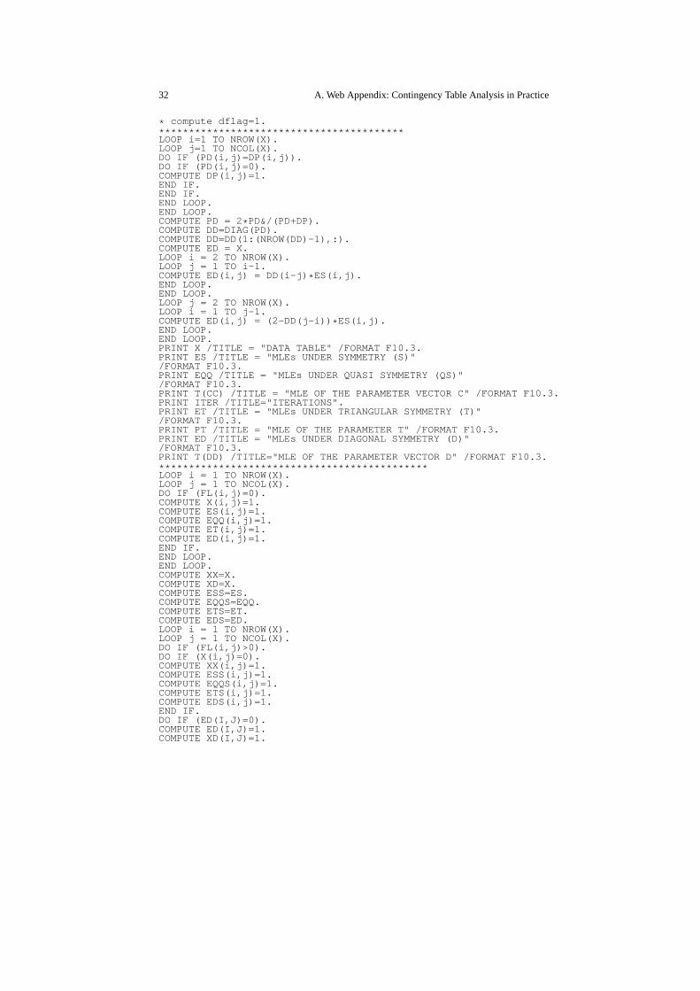
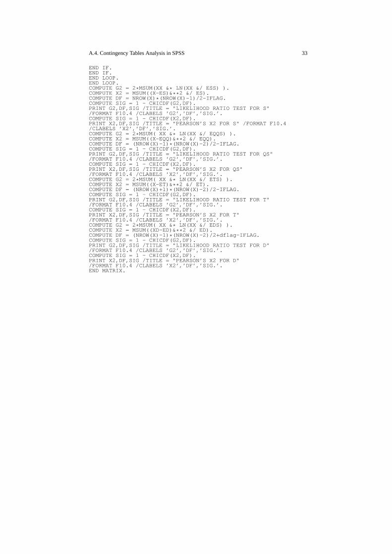
For the diagonal symmetry model D (Section 9.2.5) there is anoption to imposeequality constraints between some diagonal parameters, like in Example 9.2. In thecode that follows, the sequence of commands needed to equateparametersδ1 and
30 A. Web Appendix: Contingency Table Analysis in Practice
δ2 and correct thed f of the model accordingly, is provided as a comment. Thesecommands apply as soon as we remove the * symbols from the beginning of thecoresponding command lines. In case of different (or more) constraints, this parthas to be adjusted.
*************************************************** *** SYMMETRY, QUASI SYMMETRY, T-ASYMMETRY and D-ASYMMETRY models* for an IxI contingency table.*************************************************** ***SET MXLOOP=20000.MATRIX.GET X.COMPUTE ES = X.COMPUTE FL = X.COMPUTE IFLAG=0.LOOP i = 1 TO NROW(X).LOOP j = 1 TO NCOL(X).COMPUTE ES(i,j) = (X(i,j)+X(j,i))/2.DO IF (ES(i,j)>0).COMPUTE FL(i,j)=1.ELSE.DO IF (i<>j).COMPUTE FL(i,j)=0.COMPUTE IFLAG=IFLAG+1.END IF.END IF.END LOOP.END LOOP.COMPUTE IFLAG=IFLAG/2************************************ QUASI SYMMETRY (ITERATIVELY)***********************************COMPUTE TOLER = 10** (-3).COMPUTE RM=DIAG(X).COMPUTE CM=DIAG(X).COMPUTE CC=DIAG(X).COMPUTE RM=RSUM(X).COMPUTE CM=CSUM(X).LOOP i=1 TO NROW(X).COMPUTE CC(i)=RM(i)/(RM(i)+CM(i)).END LOOP.COMPUTE EQQ=X.LOOP i=1 TO NROW(CC).LOOP j=1 TO NROW(CC).COMPUTE EQQ(i,j)=2 * CC(i) * ES(i,j)/(CC(i)+CC(j)).END LOOP.END LOOP.COMPUTE CHECK=10.LOOP ITER = 1 TO 5000.DO IF (CHECK<TOLER).BREAK.END IF.COMPUTE EQOLD = EQQ.COMPUTE CCOLD = CC.COMPUTE CD=MAKE(NROW(CC),NROW(CC),0).LOOP j=1 TO NROW(CC).LOOP i=1 TO NROW(CC).COMPUTE CD(i,j)=CC(j).END LOOP.END LOOP.LOOP i = 1 TO NROW(X).LOOP j = 1 TO NCOL(X).DO IF (FL(i,j)=0).COMPUTE ES(i,j)=1.END IF.END LOOP.END LOOP.
A.4. Contingency Tables Analysis in SPSS 31
COMPUTE CC = RSUM(((X&* T(EQOLD))-(T(X)& * EQOLD))&/ES).COMPUTE CC=CCOLD+CC&/(RSUM((T(EQOLD)&** 2)&/(CD& * ES))-(DIAG(X)&/CCOLD)).LOOP i = 1 TO NROW(X).DO IF (CC(i)<0).COMPUTE CC(i)=CCOLD(i).END IF.END LOOP.LOOP i = 1 TO NROW(X).LOOP j = 1 TO NCOL(X).DO IF (FL(i,j)=0).COMPUTE ES(i,j)=0.END IF.END LOOP.END LOOP.LOOP i=1 TO NROW(X).LOOP j=1 TO NCOL(X).COMPUTE EQQ(i,j)=2 * CC(i) * ES(i,j)/(CC(i)+CC(j)).END LOOP.END LOOP.COMPUTE CHECK=MSUM(ABS(CC-CCOLD)).END LOOP.COMPUTE CC=CC&/EXP(MSUM(LN(CC))&/NROW(X)).
************************************ T-ASYMMETRY************************************COMPUTE PT=0.LOOP i = 2 TO NROW(X).LOOP j = 1 TO i-1.COMPUTE PT = PT+X(i,j).END LOOP.END LOOP.COMPUTE PT=2* PT/(MSUM(X)-TRACE(X)).COMPUTE ET = X.LOOP i = 2 TO NROW(X).LOOP j = 1 TO i-1.COMPUTE ET(i,j) = PT * ES(i,j).END LOOP.END LOOP.LOOP j = 2 TO NROW(X).LOOP i = 1 TO j-1.COMPUTE ET(i,j) = (2-PT) * ES(i,j).END LOOP.END LOOP.*************************************** D-ASYMMETRY**************************************COMPUTE PD=MAKE(NROW(X),NROW(X),1)-IDENT(NROW(X)).COMPUTE DP=MAKE(NROW(X),NROW(X),1)-IDENT(NROW(X)).COMPUTE PD(NROW(X),NROW(X))=1.COMPUTE DP(NROW(X),NROW(X))=1.LOOP k=1 TO NROW(X)-1.LOOP i = k+1 TO NROW(X).COMPUTE PD(k,k) = PD(k,k)+X(i,i-k).END LOOP.LOOP j = k+1 TO NROW(X).COMPUTE DP(k,k) = DP(k,k)+X(j-k,j).END LOOP.END LOOP.compute dflag=0.**************************************** equality contraints between d1 and d2 ***************************************** dflag equals the number of constraints imposed on d’s* and ’corrects’ the d.f. accordingly ****************************************** compute pd(1,1)=pd(1,1)+pd(2,2).* compute pd(2,2)=pd(1,1).* compute dp(1,1)=dp(1,1)+dp(2,2).* compute dp(2,2)=dp(1,1).
32 A. Web Appendix: Contingency Table Analysis in Practice
* compute dflag=1.*****************************************LOOP i=1 TO NROW(X).LOOP j=1 TO NCOL(X).DO IF (PD(i,j)=DP(i,j)).DO IF (PD(i,j)=0).COMPUTE DP(i,j)=1.END IF.END IF.END LOOP.END LOOP.COMPUTE PD = 2* PD&/(PD+DP).COMPUTE DD=DIAG(PD).COMPUTE DD=DD(1:(NROW(DD)-1),:).COMPUTE ED = X.LOOP i = 2 TO NROW(X).LOOP j = 1 TO i-1.COMPUTE ED(i,j) = DD(i-j) * ES(i,j).END LOOP.END LOOP.LOOP j = 2 TO NROW(X).LOOP i = 1 TO j-1.COMPUTE ED(i,j) = (2-DD(j-i)) * ES(i,j).END LOOP.END LOOP.PRINT X /TITLE = "DATA TABLE" /FORMAT F10.3.PRINT ES /TITLE = "MLEs UNDER SYMMETRY (S)"/FORMAT F10.3.PRINT EQQ /TITLE = "MLEs UNDER QUASI SYMMETRY (QS)"/FORMAT F10.3.PRINT T(CC) /TITLE = "MLE OF THE PARAMETER VECTOR C" /FORMAT F10.3.PRINT ITER /TITLE="ITERATIONS".PRINT ET /TITLE = "MLEs UNDER TRIANGULAR SYMMETRY (T)"/FORMAT F10.3.PRINT PT /TITLE = "MLE OF THE PARAMETER T" /FORMAT F10.3.PRINT ED /TITLE = "MLEs UNDER DIAGONAL SYMMETRY (D)"/FORMAT F10.3.PRINT T(DD) /TITLE="MLE OF THE PARAMETER VECTOR D" /FORMAT F10.3.*********************************************LOOP i = 1 TO NROW(X).LOOP j = 1 TO NCOL(X).DO IF (FL(i,j)=0).COMPUTE X(i,j)=1.COMPUTE ES(i,j)=1.COMPUTE EQQ(i,j)=1.COMPUTE ET(i,j)=1.COMPUTE ED(i,j)=1.END IF.END LOOP.END LOOP.COMPUTE XX=X.COMPUTE XD=X.COMPUTE ESS=ES.COMPUTE EQQS=EQQ.COMPUTE ETS=ET.COMPUTE EDS=ED.LOOP i = 1 TO NROW(X).LOOP j = 1 TO NCOL(X).DO IF (FL(i,j)>0).DO IF (X(i,j)=0).COMPUTE XX(i,j)=1.COMPUTE ESS(i,j)=1.COMPUTE EQQS(i,j)=1.COMPUTE ETS(i,j)=1.COMPUTE EDS(i,j)=1.END IF.DO IF (ED(I,J)=0).COMPUTE ED(I,J)=1.COMPUTE XD(I,J)=1.
A.4. Contingency Tables Analysis in SPSS 33
END IF.END IF.END LOOP.END LOOP.COMPUTE G2 = 2* MSUM(XX &* LN(XX &/ ESS) ).COMPUTE X2 = MSUM((X-ES)&** 2 &/ ES).COMPUTE DF = NROW(X)* (NROW(X)-1)/2-IFLAG.COMPUTE SIG = 1 - CHICDF(G2,DF).PRINT G2,DF,SIG /TITLE = "LIKELIHOOD RATIO TEST FOR S"/FORMAT F10.4 /CLABELS ’G2’,’DF’,’SIG.’.COMPUTE SIG = 1 - CHICDF(X2,DF).PRINT X2,DF,SIG /TITLE = "PEARSON’S X2 FOR S" /FORMAT F10.4/CLABELS ’X2’,’DF’,’SIG.’.COMPUTE G2 = 2* MSUM( XX &* LN(XX &/ EQQS) ).COMPUTE X2 = MSUM((X-EQQ)&** 2 &/ EQQ).COMPUTE DF = (NROW(X)-1)* (NROW(X)-2)/2-IFLAG.COMPUTE SIG = 1 - CHICDF(G2,DF).PRINT G2,DF,SIG /TITLE = "LIKELIHOOD RATIO TEST FOR QS"/FORMAT F10.4 /CLABELS ’G2’,’DF’,’SIG.’.COMPUTE SIG = 1 - CHICDF(X2,DF).PRINT X2,DF,SIG /TITLE = "PEARSON’S X2 FOR QS"/FORMAT F10.4 /CLABELS ’X2’,’DF’,’SIG.’.COMPUTE G2 = 2* MSUM( XX &* LN(XX &/ ETS) ).COMPUTE X2 = MSUM((X-ET)&** 2 &/ ET).COMPUTE DF = (NROW(X)+1)* (NROW(X)-2)/2-IFLAG.COMPUTE SIG = 1 - CHICDF(G2,DF).PRINT G2,DF,SIG /TITLE = "LIKELIHOOD RATIO TEST FOR T"/FORMAT F10.4 /CLABELS ’G2’,’DF’,’SIG.’.COMPUTE SIG = 1 - CHICDF(X2,DF).PRINT X2,DF,SIG /TITLE = "PEARSON’S X2 FOR T"/FORMAT F10.4 /CLABELS ’X2’,’DF’,’SIG.’.COMPUTE G2 = 2* MSUM( XX &* LN(XX &/ EDS) ).COMPUTE X2 = MSUM((XD-ED)&** 2 &/ ED).COMPUTE DF = (NROW(X)-1)* (NROW(X)-2)/2+dflag-IFLAG.COMPUTE SIG = 1 - CHICDF(G2,DF).PRINT G2,DF,SIG /TITLE = "LIKELIHOOD RATIO TEST FOR D"/FORMAT F10.4 /CLABELS ’G2’,’DF’,’SIG.’.COMPUTE SIG = 1 - CHICDF(X2,DF).PRINT X2,DF,SIG /TITLE = "PEARSON’S X2 FOR D"/FORMAT F10.4 /CLABELS ’X2’,’DF’,’SIG.’.END MATRIX.