ACTUARIAL RESEARCH CLEARING HOUSE 1 9 9 0 VOL, 1

INTEREST RATE VOLATILITY AND EQUILIBRIUM MODELS

OF THE TERM STRUCTURE: EMPIRICAL EVIDENCE

Mare Godin Ph.D.

Associate, Corporate Finance

Nesbitt Thomson Deacon Inc.

355, Rue St-Jacques

Montrdal, Qu6bec, Canada H2Y 1P1

(514) 282-5948

November 1987

Revised March 1988

Second Revision August 1989

Comments welcome. This paper is inspired from the empirical financial econometric portion of my Wharton PhD thesis, entitled "Equilibrium Models of the Term Structure of Interest Rates: Application to Options in Financial and Insurance Markets", submitted to the Wharton School of the University of Pennsylvania for partial fulfilment of the PhD requirements. The author wishes to thank Dave F. Babbel, Dissertation Chairman, for his helpful guidance, the members of my Dissertation Committee, the Insurance and Finance Department Faculty, Goldman Sachs & Co., for providing the data necessary for this research, and the financial support of the S.S. Huebner Foundation for Insurance Education.

199

ABSTRACT

Interest Rate Volatility and Equilibrium Models of the Term Structure:

Empirical Evidence

This p a p e r examines t h e j u s t i f i c a t i o n o f u s i n g the o n e - f a c t o r g e n e r a l

equilibrium model of Cox, Ingersoll, and Ross (CIR) [1985] to model both the

term structure of interest rates and its associated volatility. A proposed

maximum likelihood approach attempts to match both the yield curve and the

yield volatilities, using a short history of zero coupon bonds (strips) from

the U.S. government securities market. Although the CIR model appears to

match fairly well the yield curve, matching simultaneously both the yield

levels and their volatilities is found to be more difficult. This evidence

raises objections in using a one-factor model to explain yield curve

volatility behavior.

200

TABLE OF CONTENTS

I. INTRODUCTION ..................................................

2. THE COX-INGERSOLL-ROSS (1985) MODEL OF INTEREST RATES .........

2.1 The One-Factor Model .....................................

2.2 Previous Empirical Tests of the CIR Model ................

3. THE ECONOMETRIC METHODS . . . . . . . . . . . . . . . . . . . . . . . . . . . . . . . . . . . . . .

3.1 The Identification Problem of the CIR Model .............

3.2 The Maximum Likelihood Estimation Procedure .............

4. DATA SOURCES AND DESCRIPTION .................................

5. EMPIRICAL RESULTS ............................................

6. CONCLUSION . . . . . . . . . . . . . . . . . . . . . . . . . . . . . . . . . . . . . . . . . . . . . . . . . . .

R E F E R E N C E S . . . . . . . . . . . . . . . . . . . . . . . . . . . . . . . . . . . . . . . . . . . . . . . . . . .

2 0 1

I. INTRODUCTION

The aim of this paper is to examine the Justification of using the

one-factor general equilibrium model of Cox, Ingersoll, and Ross (CIR) [1985]

to model both the term structure of interest rates and its associated

volatility. A maximum likelihood approach that attempts to match both the

yield curve and the yield volatilities is proposed, using a short history of

zero coupon bonds (strips) from the U.S. government securities market.

Although the CIR model appears to match fairly well the yield curve, the

simultaneous matching of both the yield levels and their volatilities is found

to be more difficult. This evidence raises objections in using a one-factor

model to expalin yield curve volatility behavior.

The paper is organized as it follows. Section 2 describes the nature of

the CIR model of interest rates, along with the empirical investigations of

that model. Section 3 explains the statistical estimation method used to

solve the particular identification problem of the CIR model. A maximum

likelihood procedure is used and the estimation, and asymptotic properties are

presented. Section 4 describes the financial data used for the estimations.

Section 5 presents the results and analyzes the likely causes of the model's

failure to explain simultaneously both the yield curve and its associated

volatility using the same one-factor model. Section 6 concludes.

202

2. THE COX-INGERSOLL-ROSS (1985) MODEL OF INTEREST RATES

2.1 The One-Factor Model

In Cox, Ingersoll, and Ross [1985], thereafter CIR, the problem of

determining the term structure is posed as a problem in general equilibrium

theory. A rational asset pricing model to study the term structure of

interest rates is used. The current prices and stochastic properties of all

contingent claims, including bonds, are derived endogenously. Anticipations

of future events, risk aversion, investment alternatives, and preferences

about the timing of consumption all play a role in determining the term

structure. The model thus includes the main factors traditionally mentioned

in a way which is consistent with maximizing behavior and rational

expectations.

The dynamics of the simplest form of the CIR [1985] model for the interest

rate process are given by

(i) dr - ~(0-r) dt + o Jr dz ,

where ~, #, a 2 are constants, with ~8>0 and o2>0. The model thus assumes that

the term structure is fully specified by the instantaneous riskless rate

r(t). For 6>0 and ~>0, this corresponds to a continuous time first-order

autoregressive process where the randomly moving interest rate is elastically

pulled toward a central location or long-term value, 0. The parameter

determines the speed of adjustment.

Let's recall the valuation equation of a default-free discount bond,

P[r,t,T], that pays one unit at time T, ~-T-t periods from now. Using the

drift and variance formulae for r as well as the term for the factor risk

203

premium, ~, the fundamental equation is given by

(2) (I/2)°2rPrr + m(0"r)Pr + Pt -ArPr -rP - O.

with the boundary condition P(r,T,T) - I. Ito's Lemma gives the expected price

change for the bond as

(3) (I/2)a2rPrr + m(8"r)Pr + Pt

thus ArP r+rP is the expected return on the bond, and r+ArPr/P is the rate of

that expectation. Obviously, ~-ArPr/P is the term premium on the bond, and

can be written in two parts as

(4) ~-(~r) (Pr/P)

where lr is the covariance of changes in r with the percentage changes in

"market portfolio", and Pr/P is the elasticity with respect to the interest

rate, or the negative of the modified price duration. Since Pr<O, z>0 if ~<0

(i.e. negative correlation with optimally invested wealth (the market

portfolio).

In the present single factor model, the returns on all assets are

perfectly correlated to the extent they are all exposed to the risk inherent

in the interest rate process. The instantaneous interest rate on the zero

coupon bond can be written as

(5) dP/P - [~(~-r)Pr/P + Pt/P + (i/2)o2rPrr/P] dt+ oJr Pr/P dz

- ~(r,t,T) dt + u(r,t,T) dz.

By taking the relevant expectations, and using the Brown and Dybvig [1986]

notation, the solution of the fundamental equation is of the form

(6) P[r,t,T]- AIr,T]* e "B[t'T]r

where for ~ - T~t,

204

( T a )

( 7 b )

where

(7c)

(7d)

(7e)

AIr,T]- { ~lexp(~2 T) / (~2[exp(~l~)-l]+~ I) }

B[t,T]- [exp(@ir)-i ] / [(~2[exp(~lV)-l]+~l)]

~i - { (~+A)2 + 2a2 } 1/2

~2 - (~+~ + ~I ) / 2

2 ~3 - 2~8 / a .

~3

2.2 Previous Empirical Tests of the CIR Model

In a recent paper, Brown and Dybvig [1986] tested the nominal form of the

one-factor CIR model of the term structure on 373 cross- sections of monthly

US Treasury, default free coupon bond prices data from 1952 through 1983. Each

cross-section was used to produce maximum likelihood estimates of the

identifiable parameters. Using their cross-sectional methodology, they

pointed out that the CIR [1985] model was not fully identified. Nevertheless,

they came out with estimates of the short-rate of interest (which was treated

as an additional parameter), the long-term rate or mean reversion rate, and

the variance parameter.

Stambaugh [1986] offered another test of the Cox-Ingersoll-Ross [1985]

model by focusing on the nature of the expected excess returns. In such a

model, the expected excess returns are linear functions of forward premiums,

where the number of latent variables captured by the forward premiums equals

the number of state variables in the pricing relation. Stambaugh pointed out

that when the maturities of the forward premiums match those of the excess

returns, the number of state variables required to describe expected returns

can appear to be large due to measurement errors. An alternative set of

forward premiums with non-matching maturities is postulated to reduce the

205

problems arising from measurement error. Tests of the number of latent

variables in expected returns on U.S. Treasury bills were performed in a

Generalized Method of Moments (GMM) framework and rejected a slngle-variable

specification of the term structure. But Stambaugh provided some evidence

that two or three latent variables appear to describe expected returns on

bills of all maturities. Expected returns estimated using two latent

variables vary with business cycles in a manner similar to what Fama [1986]

observed for forward rates for the full range of maturities. Nevertheless,

Stambaugh concluded by affirming chat expected returns on U.S Treasury bills

appear to change over time in a manner that is consistent with parsimonious

models of the term structure, such as models developed by Cox, Ingersoll, and

Ross [19851 .

3. THE ECONOMETRIC METHODS

In the nominal form of the CIR [1985] model, the successful identification

and estimation of the parameters are sufficient to price nominal bonds of any

maturity. Moreover, the yields on these bonds are perfectly positively

correlated. This follows from

(Sa)

(8b)

(8c)

Pt(r,~) - A(T) exp{-B(T)r(t)} ,

Yt(r,~) - - In[Pt(r,~)]/, - a(f) + b(~)r(t) ,

a(T) - -In[A(~)]/~, b(f) - B(~)/r ,

(Sd) COV[Yt(r,,l),Yt(r,~2) ] - b(~l)b(,2)VAR[r(t) ] ,

(8e) VAR[Yt(r,Ti) ] - b(Ti)2VAR[r(t) ] ,

where COV and VAR are unconditional covariances and variance operators, and

where VAR[r(t)] - o2r(t).

206

In this section, we will lay out the econometric method used to estimate

the parameters of the interest rate model. Both the generalized method of

moments and the maximum likelihood estimation procedures will be explained,

along with their statistical properties and inference. A statistical testing

methodology for contingent claims models will be developed, using the

principle of invariance. But before, let's address the identification problem

of the CIR [1985] model, as suggested by Brown and Dybvlg [1986].

3.1 The Identification Problem of the CIR Model

In practice, what we observe is the nominal price of a discount bond at

date t for a dollar deliverable at t+r. In a single model of the term

structure of interest rates, if the state variable is observable, and if there

are several bonds of different maturities to permit identification of the

problem, then simply equating the functional form with the observed discount

bond prices or yields, at a point in time, would represent a way to estimate

the parameters of the model from a cross-section of securities, using

non-linear regression techniques. To that effect, Gibbons and Ramaswamy

[19861 , in their two-factor model of the real term structure, add

Even without observing the state variable, non-linear cross-sectional regressions may allow identification and estimation of the underlying parameters as long as the state variables are treated as additional parameters. However, it is not clear how to link the time series properties of the state variables to the estimated parameters [p. 7].

Brown and Dybvig [1986] mentioned an identification problem,

associated with the GIR model. Originally cast using four parameters

and a state variable, or five parameters, (~, 6, A, o, r), the model

cannot be separately identified, using cross-sectional data. The reason

lies in the appearance of ~ and A as ~+A almost everywhere in the model,

so that, when considering a single cross-section, the four parameters

(~, 6, A, o) can be expressed as three (41, 42, 43). One way to

207

alleviate the problem is to impose the no-arbitrage condition, the

so-called Local Expectations Hypothesis, i.e set A-0.

Another way to solve the identification problem is to take advantage

of the availability of the dynamic specification of the single forcing

variable, the instantaneous riskless rate, r(t). Specifically, one can

observe the term structure at different points in time, the so-called

time series approach, and make use of the availability of a functional

form within the CIR model for the relevant densities of the unobservable

forcing variable, r. In doing so, our system becomes "overidentified",

since a single forcing exogenous variable is used to explain two sets of

endogenous variables. One is then able to exploit this availability in

testing the overldentifying restrictions and arriving at parameter

estimates.

In estimating a nonlinear system related to the proposed one,

Gibbons and Ramaswamy [1986] used the Generalized Method of Moments

(GMM) first developed by Hansen [1982] and employed in Hansen and

Singleton [1983], Brown and Gibbons [1985] and elsewhere. Gibbons and

Ramaswamy used the restrictions on the population first and second

moments of the CIR model to identify the parameters. The first moment

restrictions are given by the functional form of the CIR model for the

discount bonds, taken separately, at the same given point in time. The

second moment restrictions, or cross and autocovariances, are given by

the functional form of the variance and autocovariance functions of the

model, for two discount bonds, identical or different, taken at two

different points i_nn time.

Our approach somewhat differs form the one taken by Gibbons and

Ramaswamy [1986], but nevertheless, carries the essential of the moment

matching idea. In a first step, the term structure of interest rate,

i.e. the yield curve for discount securities of different maturities,

is calculated at a given point in time, assuming starting values that

would made mean reversion possible (~,0>0). In a second step, we use

208

these estimates of the yield curve equation as initial estimates, 410,

420, and o0, for the yield curve volatility or second moment

restrictions. Alternatively, we can use these initial estimates to

estimate jointly both the yield and yield volatilities simultaneously,

by using also a non-linear estimation technique. In that case, the

mlnimand uses both the errors in the yields and in their volatilities.

The One-Step Theorem ensures us that, for the parameters estimated in

the first procedure, i.e. 41, 42 , and a, the final estimates for those

estimates have the same statistical properties as the estimates of the

first step.

The yield curve volatilltles are measured using the daily yield

observations of the recent, past trading days. Usually, a three-month

period, consisting of approximately 60 trading days is chosen; but

periods such as one month (last 20 trading days), or one year (252

trading days) could be chosen. Different methods of estimations could

be chosen to obtain a standard deviation of the yield estimates, the

proxy for the volatility. Usually, the simple maximum likelihood

estimate of the standard deviation will be chosen. If the data is

thought to be unreliable, a robust estimate, one that minimizes the

absolute mean deviation, as opposed to the square of the deviations,

could be used.

Working with daily bond price data also uncovers the problems

associated with nonsynchronous trading, which is thought to cause the

observed autocorrelations in daily returns on asset prices. Fama [1970]

found slightly positive average autocorrelations in examining daily

security returns with a lag of one day and no empirical evidence of

significant autocorrelatlons for higher lags. Also, daily market- index

returns exhibit a pronounced positive first- order autocorrelatlon.

This index phenomenon has been called the Fisher effect since Lawrence

Fisher [1966] hypothesized its probable cause. Hence a correction for

auto-correlation of daily errors in yields would be used, in calculating

the second moments of the yield relationships.

209

Since the volatility restrictions do not depend on the

mean-reversion parameter, 6 (CIR notation), or equivalently, ~3

(Brown-Dybvig notation, thereafter BD), values for the parameters 41,

42, and o can be found by a non-llnear estimation procedure.

3.2 The Maximum Likelihood Estimation Procedure

The maximum likelihood estimation procedure proposed here, which

differs from the ones used in estimating the CIR model by Brown and

Dybvig [1986] and Gibbons and Ramaswamy [1986], nevertheless carries the

essential of the moment matching idea. It exploits the dynamic

specification of the CIR model in testing the overidentifylng

restrictions and arriving at parameter estimates. Specifically, we

still want to minimize the quantity (mlnlmand)

(9) nini.ize ~(~) - gT(~)'o-l&r(~)

#~B

where ~-~(r,~,8,o,A) are the model parameters, ~ is a weighting matrix,

the asymptotic covariance matrix of the vector of sample moment

conditions, gT(@); the vector ET(~) is now defined by stacking the

vectors from the relations on the first moment (the yield curve) and the

second moment (the yield curve volatility):

(10a) hlt(rl;~) m yt(,i) - a(¢i) - b(ri)r(t )

(10b) h2t(ri;~) - SD[Yt(rl) ] - b(,i)SD[r(t) ] , i, j- 1 ..... n

where SD is the unconditional (relative) standard deviation operator,

and where n is the number of available maturities for the pure discount

instruments. In practice, the unconditional standard deviation is

estimated using recent daily observations, correcting for the Fisher

effect (first autocorrelation, due to nonsynchronous trading). Since

210

hit and h2t are assumed to be normally distributed, our procedure

involves choosing ~ from a feasible region B to minimize these

deviations from the model. Note that the state variable, r(t), can be

either left outside of the estimation, if it is observable with

precision at the valuation date, or can be incorporated in the

maximization procedure, as an additional parameter.

The estimation problem we face is the joint estimation of the system

(~,n). Usual applications of the MLE require a two-step procedure to

find ~, where ~ is first set equal to the identity matrix, and the

resulting set of estimates for ~ are used to construct a second

matrix, different from the identity matrix. In the procedure described

above, the special structure of the orthogonality conditions, ht(~), is

used to avoid this first step. Looking at the special nature of the

estimation problem, the assumption of serially uncorrelated ht(~), due

to a rationality assumption that agents use all past information, would

be reasonable. There is no reason, a priori, to expect the errors in

the yield curve matching, the hit condition, could be correlated with

the ones in the yield curve volatility matching, the h2t condition, nor

there is any reason to expected correlations in the two hits or h2ts of

different maturities. For these reasons, the diagonal structure will be

adopted for the weighting matrix. The asymptotic justification for MLE

only requires that the weighting matrix be a consistent estimator of the

asymptotic variance- covariance matrix for h(~).

The covariance matrix of the asymptotic distribution of the MLE

estimator for ~ can then be consistently estimated by:

* - -i (lla) Var(~*) - [Dr(~ )~ ID(~*)] ,

* T-I (llb) D(~ ) - ~t aht/a~ I~_~*

Asymptotic tests and inference can be conducted on the MLE estimates,

using the well known three asymptotic tests mentioned in Engle [1984];

these are the likelihood ratio test (LRT), the Wald's test, and the

211

Lagrange Multiplier (124) or Rao test. All three tests can be shown to

have the same limit Chisquare distribution, x2(q), under the null

hypothesis, where q is the number of parameters to estimate. In our

case, Wald's test would be the easiest to use, since it requires only to

estimate the score and Hessian functions under the unrestricted form.

This contrasts with the Lagrange Multiplier test, which requires a new

estimation for each restricted values of the parameter, and the LRT,

which requires both restricted and unrestricted estimations.

4. DATA SOURCES AND DESCRIPTION

The empirical results reported in this research are based on a cross-

section of data on the Government securities market. These data can be

obtained from several sources, such as the CRSP tape and the Wall Street

Journal. Using the methodology described previously, we estimate the

parameters of the term structure of interest rates on the basis of data on the

prices of U . S . Treasury issues trading at a given point in time. Treasury

issues, other than Treasury bills, are coupon bonds and can be represented in

the model if we regard each as the sum of a series of discount issues

corresponding to each coupon payment, plus a discount issue corresponding to

the terminal payment on the bond. In fact, this decomposition of coupon bonds

into coupons and principal repayment of different maturities make possible the

estimation of the highly non-llnear bond price function with only a handful of

coupon bonds, using a cross-sectional sample of bond prices at a given point

in time.

Data on US Treasury securities prices were obtained from the Goldman,

Sachs & Co. database in August 1986. Those prices were either the trading

prices or the mean of the bid and ask price quotations where trading prices

were otherwise not available, plus the accumulated interest (for coupon bonds)

as of that date. For each price, the corresponding time to maturity as well

as (for coupon bonds) the coupon payments, number of payments remaining and

212

time to next payment were also recorded.

The market for pure discount (zeros or strips) bonds has expanded

dramatically over the last years. These pure securities are available at

maturities varying between three months and thirty years. So, the universe of

U,S. pure discount securities offers a cross- section of between Ii0 and 120 i

securities, traded at a given time. For this reason, and because the

liquidity problem associated with current versus seasoned issues is not as

important an issue (in fact, to some extent, all zeros are equally illlquld), 2

we will use, when available, data from the pure discount securities.

5. EMPIRICAL RESULTS

The estimation of the term structure of interest rates, under the CIR

[19851 model involves a two-step procedure, as described in a previous

section. In a first step, the yield curve is estimated using the universe of

traded US Treasury Strips at a point in time. This yields initial estimates

of the parameters of interest ~ - [r ~I ~2 ~3 ]' as proposed by Brown and

Dybvig [1986]. The results of the estimation are shown in Graph I.

I. The author recognizes that a nonsynchronous trading problem might exist here. Typically, as in the case of the coupon securities, some bonds are traded more actively than others. In that case, at the end of the day, bonds that did not trade are adjusted up or down before being inputted in the data base. Nevertheless, the pure discount securities offer an analytically tractable way of imposing moment restrictions to identify the parameters of the term structure.

2. Gibbons and Ramaswamy [1986] observed the presence of these stripped, single payment certificates, derived from coupon- bearing Treasuries, but felt that, for their 1964-1983 period of observation, they lacked a sufficient history. Our approach, while raising the problems associated with daily data, does not require a long history of stripped securities.

213

I~D

.T.

9 0

Graph 1

Comparison of Acfual fo Fitfed Sfrip Yields Eslimaled using US Treasury Strips Universe - DATE: 0 8 / 2 8 / 8 6

v

0

8 ~

8 0

7 5

7 0

8 b

6.0

5 0

0 . 0

~ p ~ . . . . . - O o o o o

/ oP f / c ~ 0

/ o p P P

/2

f o Acluol Yield I _ Filled Yield

r - T - - - - , - - - , - - - - r . . . . I . . . . , - - ~ - . . . . . . 7 - [ - - - - , i - 2 2 ~ n ~ 1 2 - ' - - 2.5 5.0 7 5 10.0 12.5 15.0 17.5 20.0 22.5 25.0 27.5 .',0.0

Malurily (in years)

The point estimates of the cross-sectional estimation were

r - 0.05278, 41 - 0.41436, 42 - 0.40736, ~3 - 11.998 .

As Brown and Dybvig noted, it is impossible to separately estimate the five

parameters of interest ~ - [r m A o 0], using only a cross-sectlon, unless the

Local Expectations Hypothesis (LEH) assumption is used. Using the

transformation mentioned in Brown and Dybvig [1986], mainly

(7c) ~I - ( (~+A)2 + 2a2 } 1/2

(7d) #2 - (~+A + 41 ) / 2

2 ( T e ) 4 3 - 2~9 / ~ ,

the identification problem is highlighted by the following system of 2

equations with three unknowns

( 1 2 a ) ~e - 0.03378

(12b) ~+A - 0.40036.

Hence, in a second-step, the yield volatility curve is estimated using a

time-series of daily yields on the universe of traded US Treasury Strips for

the past 60 trading days prior to the valuation date. The volatillties were

adjusted for the econometric problems mentioned in a previous chapter, The

results of the volatility estimation are shown in the first fitted curve

(Fitted Volatility-l) of Graph 2,

215

I 3 0 0 -

Graph 2

Comparison of Actual Io Fitted Strip Yield Volatilities Estimated using US Treasury Sfrips Universe - DATE: 0 8 / 2 8 / 8 6

o 0 > "u

>-

2bO

20,0

150

I0 .0

50

O 0

O0

~ c o r P ; M . . 4 )

\ \

\

o Actual Volatility Fitted Volatility_-1 Fitted v o l a f i ! i t y - 2

~ ~ m . ~ r ~ o o ° o o o o o o o o

n - . . . . . . r . . . . I - - - - ]

2.5 5.0 2.5 I0,0 12.,5 1,5.0 17,5 20 .0 2 .5 25.0 2 .5

Maturity (in years) 30.0

Note that the estimates are biased. Several initial estimation points were

tried, but, in all cases, the resulting likelihood estimates were found to be

downward biased. This is perceived to be due to the intrinsic limitation of

the one-factor model used in this research. Nevertheless, the corresponding

"underidentified" system in that case was

(13a) ~O - 0.00157

(13b) ~+A - -0.01464.

Note also that the long-term mean reversion parameter, 0, is a parameter

of interest only in the yield curve matching, and not in the yield volatility

curve matching. Since the long-term mean reversion parameter, O, was found,

in the yield curve matching, to be of the order of 8.5%, this would imply the

following point estimates for the speed of adjustment and the risk premium

parameter in the volatility matching: ~ -0.0185, A --0.0331. If this point

estimate were to be significant and correct, the excess return on a strip of

maturity r- T-t would be -% f. This is obtained from the equilibrium rate of

return relationship shown previously in the risk premium section. Recalling

that

(14) ~(r,t,T)- ~(r) - r + A (r,t) Pr/P - r + A r Pr/P - r + A Dmo d ,

and since the duration of a zero is equal to its maturity, this would have

mean that the expected return on a 30-year zero would have been of the order

of 5+(3.31)30 - 104%. Since there is no reason a priori to expect the excess

return on a 30-year zero to be ten times as much as the one on a 3°year zero,

and 30 times as much as the 3.3% excess return on a 1-year zero, the joint

estimation of the yield curve and yield curve volatilities was redone, using

the initial estimates of the yield curve only estimation and the LEH

assumption. The results are found in Table 1

217

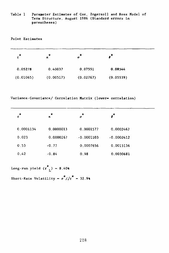
Table 1 Parameter Estimates of Cox, Ingersoll and Ross Model of Term Structure, August 1986 (Standard errors in parentheses)

Point Estimates

r ~ o #

0.05278 0.40037 0.07551 0.08544

(0.01065) (0.00517) (0.02767) (0.05539)

Variance-Covarlance/ Correlation Matrix (lower- correlation)

* * * 9: r ~ a @

0.0001134 0.0000013 0.0001577 0.0002462

0.023 0.0000267 -0.0001103 -0.0002412

0.53 -0.77 0.0007656 0.0015136

0.42 -0.84 0.98 0.0030681

Long-run yield (r L ) - 8.40%

Short-Rate Volatility - o*/Jr* - 32.9~

218

The yield curve matching was left almost unchanged. But the yield curve

volatility matching is found to be much worse. This is shown in the second

fitted curve (Fitted Volatility-2) of Graph 2, where the second fitted

volatility is obtained from the final maximum likelihood estimation. The

downward sloping volatility curve was observed by other researchers, such as

Black, Derman, and Toy [1987] and is often associated with the mean reverting

behavior of the short term interest rate:

"In our model, today's long rate reflects expected future short rates, and today's long-rate volatility reflects expected future short-rate volatillties. Therefore, when we match today's term structure to expected future short rates, our model's future short rate volatility must also decrease with time. In our model... the expected short rate volatility depends only on time and not on the short rate itself. If future short rate volatilities decrease with time, then high future short rates become less likely as time goes by. This damping out of fluctuations in high short rates is equivalent to mean reversion. So, in our model the declining volatility curve is equivalent to mean reversion. [p. 14]

Even if, as in the CIR model, the expected short rate volatility

depends not only on time, but also on the short rate itself, these

conclusions somewhat remain the same. Specifically, if A and 8 are

positive, then one can show that

(B.5) lim -i B(,) - 0

i.e. in a one-factor model, the yield variability of the long-term zero

coupon bond tends to zero, implying a declining yield volatility curve.

219

6 . CONCLUSION

This paper examined the justification of using the one-factor general

equilibrium model of Cox, Ingersoll, and Ross (CIR) [1985] to model both the

term structure of interest rates and its associated volatility. A maximum

likelihood approach attempted To match both the yield curve and the yield

volatilities, using a short hi: :ory of zero coupon bonds (strips) from the

U.S. government securities market. Although the CIR model appears to match

fairly well the yield curve, matching simultaneously both the yield levels and

their volatilities is found to be more difficult.

The evidence provided here r, ised objections in using a one-factor model

to model yield curve volatility iehavior. In a related study to this paper,

Stambaugh [1986] tested the numh~ r of latent variables in expected returns on

U.S. Treasury bills, using a Generalized Method of Moments (GMM) framework and

rejected a single-variable speci: :cation of the term structure. But Stambaugh

provided some evidence that tw~ or three latent variables appear to describe

expected returns on bills of all maturities. Nevertheless, Stambaugh and most

researchers agree that expected returns on U.$ Treasury bills appear to change

over time in a manner that is consistent with parsimonious models of the term

structure, such as models develo~.ed by Cox, Ingersoll, and Ross [1985].

We have discussed here one limitation of the Cox, Ingersoll, and Ross

[1985] model, which imposes restrictions on the joint determination of yield

curves and yield volatilitles. Because the same parameters determine both the

yield curve and the yield curve volatilltles, subtle combinations of term

structure and volatilities are iN:,ossible. For instance, a model where mean

reversion occur could not poss:',ly have a rising yield volatility curve.

Nevertheless, one- and two-facto: models of the term structure remain popular

because of their tractability.

220

REFERENCES

i. Black, Fisher, Emmanuel Derman, a n d William Toy, [1987], "A One-Factor Model of Interest Rates and Its Application to Treasury Bond Options". Internal memorandum, Goldman, Sachs & Co.

2. Brown, David P. a n d Philip H. Dybvig, [1986], "The Empirical Implications of the Cox-lngersoll-Ross Theory of the Term Structure of Interest Rates", Journal of Finance 41, 617-30.

3. Brown, David P. and Michael R. Gibbons, [1985], "A Simple Econometric Approach for Utility- Based Asset Pricing Models", Journal of Finance 40, 359-381.

4. Cox, J., J.E. Ingersoll, Jr., and S.A. Ross, [1985], "A Theory of the Term Structure of Interest Rates", Econometrlca, Vol. 53, 2. : 385-407.

5. Engle, R., [1984], "Wald, Likelihood Ratio, and Lagrange Multiplier Tests in Econometrics", in Handbook of Econometrics Vol. II, Griliches and Intriligator, eds., chap. 13.

Fama, E.F., [1970], "Efficient Capital Markets: A Review of Theory and Empirical Work", Journal of Finance 15 (May), 383-417.

Fisher, Lawrence, [1966], "Some New Stock Market Indexes", Journal of Business 39 (January), 191-225.

Gibbons, Michael R., and Krishna Ramaswamy, [1986], "The Term of Interest Rates: Empirical Evidence", Working paper, University and University of Pennsylvania, December.

Structure Stanford

Hansen, Lars P., [1982], "Large Sample Properties of Generalized Method of Moments Estimators", Econometrica 50, 1029-1054.

IO. Hansen, Lars P. and Kenneth J . Singleton, [1982], "Generalized Instrumental Variables Estimation of Nonlinear Rational Expectations Models", Econometrlca, 50, 1269-86; Errata, 52, 267-8.

Ii. Lo, Andrew W., [1986], "Statistical Tests of Contingent- Claims Asset- Pricing Models: A New Methodology", Journal of Financial Economics 17, 143-173.

12. Stambaugh, R.F., [1986], MThe Information in Forward Rates: The Implications for Models of the Term Structure", Working paper, Graduate School of Business, University of Chicago, September.

221

222