Predictive energy management for hybrid electric aircraft propulsion

systems

Martin Doff-Sotta∗, Mark Cannon, Marko Bacic

November 15, 2021

Abstract

We present a Model Predictive Control (MPC) algorithm for energy management in aircraft with hybridelectric propulsion systems consisting of gas turbine and electric motor components. Series and parallelconfigurations are considered. By combining a point-mass aircraft dynamical model with models of electricallosses and losses in the gas turbine, the fuel consumed over a given future flight path is minimised subjectto constraints on the battery, electric motor and gas turbine. The optimization is formulated as a convexproblem under mild assumptions and its solution is used to define a predictive energy management controllaw that takes into account the variation in aircraft mass during flight. We investigate the performance ofalgorithms for solving this problem. An Alternating Direction Method of Multipliers (ADMM) algorithm isproposed and compared with a general purpose convex interior point solver. We also show that the ADMMimplementation reduces the required computation time by orders of magnitude in comparison with a generalpurpose nonlinear programming solver, making it suitable for real-time supervisory energy managementcontrol.keywords: Alternating Direction Method of Multipliers (ADMM), Convex Programming, Energy Manage-ment, Hybrid Aircraft, Model Predictive Control (MPC).

1 Introduction

Aviation currently contributes to around 2% of current world-wide human-made CO2 emissions, but demandfor air travel is predicted to grow significantly. The aviation industry is committed to realising this growthsustainably with a drastic reduction of CO2 emissions by 2050. One avenue identified to achieve this ambitiousgoal is the development of greener aviation based on new propulsion concepts.

Aircraft equipped with turbo-electric and hybrid electric powertrains are considered in [2, 17, 28] where itis shown that reductions in emissions and energy savings can potentially be achieved. In [28], simulations of acommercial airliner with boundary layer ingestion and a turbo-electric propulsion system predict mission fuelburn savings of up to 7% relative to a conventional propulsion system. A distributed electric propulsion conceptfor the transonic cruise range proposed in [22] is likewise expected to provide a 7% reduction in fuel. Potentialenergy savings were demonstrated for a concept year-2030 aircraft equipped with a parallel-hybrid propulsionsystem combined with an all-electric propulsion system in [2].

Hybrid-electric propulsion systems rely on energy management controllers to allocate power demand betweenthe different components of the powertrain. The energy management problem can be tackled with heuristicstrategies such as peak-shaving schemes [26], charge-depleting-charge-sustaining policies [7], approaches basedon state machines [24] and rule-based fuzzy logic [6]. More sophisticated suboptimal control strategies have alsobeen proposed, for example using neural networks [20] and neuro-fuzzy adaptive control [14].

Optimisation techniques that seek to minimise a cost function (such as fuel consumption) have also beenproposed for energy management problems. For example, the so-called equivalent fuel consumption minimisationstrategy is widely used in hybrid fuel cell systems [11]. Globally optimal policies have been computed offlineusing dynamic programming [4,15,18] but the computation required is prohibitive for real-time implementation.Other approaches based on H∞ control [21] and optimal adaptive control [19] have also been proposed. Apopular framework for energy management problems in electric and hybrid-electric ground vehicles is ModelPredictive Control (MPC) [5, 10, 16]. The energy management problem is formulated as a receding-horizonconstrained optimisation problem, and an optimal power split is found at each discrete time step. Since MPCis a feedback control strategy that is updated with information on the system state at each time step, it can

∗M. Doff-Sotta, M. Cannon and M. Bacic (on part-time secondment from Rolls-Royce plc) are with the Control Group, Universityof Oxford, Parks Road, Oxford, OX1 3PJ, United Kingdom (e-mail: martin.doff-sotta@eng.ox.ac.uk, mark.cannon@eng.ox.ac.uk,marko.bacic@eng.ox.ac.uk).

1

arX

iv:2

103.

0790

9v2

[m

ath.

OC

] 1

2 N

ov 2

021

provide robustness to modelling uncertainty and prediction errors. Although MPC has been proposed forenergy management problems in hybrid-electric aircraft [8, 23], none of these approaches considered losslessconvexification of the nonlinear programming problem.

A convex energy management formulation is proposed in [7], which considers a parallel-hybrid aircraft withnonlinear constraints in a model predictive control framework. Fuel consumption is predicted over a future flightprofile and is minimised subject to constraints on state, trajectory and physical limitations of the componentsof the propulsion system. The associated receding-horizon nonlinear programming problem is posed as a convexprogram and solved using the general-purpose convex optimisation framework CVX [12].

This paper extends the results in [7] to series-hybrid architectures and describes a specialised ADMM solverfor efficient online optimisation. The paper is organised as follows. Mathematical models of the powertraincomponents and aircraft dynamics are developed in Section 2. Energy management problems for series andparallel configurations are stated as receding-horizon optimisation problems in Section 3. Section 4 presents aseries of simplifications that yield convex formulations of these problems. In particular, a unified formulation isproposed for both powertrain configurations. The ADMM solver is presented in Section 5 and its performanceand potential for real-time implementation are discussed in Section 6. Conclusions are presented in Section 7.

2 Modelling

This section derives models of the aircraft dynamics and powertrain components (battery, electric motor, gasturbine etc.), which will be used to formulate the energy management problem as a model-based optimisationproblem.

We consider a hybrid electric aircraft propulsion system with either a series or parallel topology. When thepower output demand is negative, which may occur for example while the aircraft is descending, we consider thepossibility of using the same powertrain to generate electrical energy (i.e. operating in a “windmilling” mode)in order to recharge the battery. In practice a variable-pitch fan would be required for this functionality, whichwould increase complexity.

2.1 Aircraft Dynamics

The aircraft motion is constrained by its dynamic equations. Assuming a point-mass model [25] and referringto Figure 1, the equilibrium of forces yields

md

dt(−→v ) =

−→T +

−→L +

−→D +

−→W,

where −→v is the velocity vector, m the instantaneous mass of the aircraft,−→T the vector of thrust,

−→L and

−→D are

the lift and drag vectors and−→W is the aircraft weight.

−→T

−→D

−→W

−→L

−→v αγ

Figure 1: Aircraft forces and motion.

Using the coordinates (v,γ), where v is the velocity vector magnitude and γ is the flight path angle, and

projecting the vector equation in wind axes along the drag vector−→D yields

md

dtv +mg sin γ = T cosα− 1

2CDρSv

2.

Here S is the wing area, ρ is the density of air, g is acceleration due to gravity, CD = CD(α) the drag coefficient

and α the angle of attack. Projecting along the lift vector−→L yields

mvd

dtγ +mg cos γ = T sinα+

1

2CLρSv

2,

where CL = CL(α) is the lift coefficient.

2

The drive power is given as follows

Pdrv =−→T · −→v = m

d

dt(1

2v2) +

1

2CDρSv

3 +mgv sin γ.

2.2 Hybrid Propulsion System

2.2.1 Parallel architecture

In the parallel architecture (T = P), a gas turbine producing power Pgt is mechanically coupled with an electricmotor with power output Pem in a parallel arrangement (Fig. 2). These two power sources are combined to givethe power output of the propulsion system, Pdrv, via

Pdrv(t) = Pgt(t) + Pem(t),

where 100% efficiency in drivetrain components is assumed.

Battery ElectricBus

Motor/Gen.

FuelGas

Turbine

Fan

Pb Pc Pem

ϕ Pgt

Pdrv

Figure 2: Parallel-hybrid propulsion architecture.

2.2.2 Series architecture

In the series architecture (T = S), the propulsion system power output Pdrv is delivered by an electric motortaking electrical power Pel from two sources: a battery with effective power output Pc and a turbo generatorset (gas turbine in series with an electric generator) with power output Pgen (Fig. 3). The power balance isgiven by

Pel(t) = Pgen(t) + Pc(t).

Battery ElectricBus

Motor/Gen.

Fuel GasTurbine

Gen.

Fan

Pb Pc

Pel

ϕ Pgt Pgen

Pdrv

Figure 3: Series-hybrid propulsion architecture.

2.3 Battery

The battery is modelled as an equivalent circuit with internal resistance R and open-circuit voltage U , so thatthe input-output map between its chemical power Pb and the effectively delivered electrical power Pc is givenby [13]

Pb = g(Pc

),

=U2

2R

(1−

√1− 4R

U2Pc

),

where U and R are assumed constant [9]. The evolution of the battery state of charge (SOC) E(t) is given by

E = −Pb (1)

and E(t) is subject at all times to upper and lower bounds

E ≤ E ≤ E.

3

2.4 Gas turbine

The rate of change of mass of the aircraft is given by

m = ϕ = −f(Pgt(t), ωgt(t)), (2)

where ϕ is the rate of fuel consumption and f(Pgt, ωgt) is a piecewise-quadratic function of the gas turbinepower output Pgt and shaft rotation speed ωgt. We assume that f(·) can be determined empirically from fuelmap data in the form

ϕ = f(Pgt, ωgt),

= β2(ωgt)P2gt + β1(ωgt)Pgt + β0(ωgt),

with β2(ωgt)≥0 and β1(ωgt)>0 in the operating range of ωgt. The power Pgt and shaft rotation speed ωgt arelimited by

P gt ≤ Pgt ≤ P gt,

ωgt ≤ ωgt ≤ ωgt.

These limits apply to both parallel and series configurations, and in the latter case they constrain the turbogenerator set.

2.5 Electric motor

In the parallel configuration, the electric motor input-output map between input electrical power Pc and effectivemechanical power Pem is modelled by a piecewise-quadratic function

Pc = h(Pem(t), ωem(t)),

= κ2(ωem)P 2em + κ1(ωem)Pem + κ0(ωem),

where ωem is the electric motor shaft rotation speed and κ2(ωem) ≥ 0, κ1(ωem) > 0 for all ωem in the operatingrange. The function h(·) can be determined empirically from electric motor loss data. The limitations on theelectric motor power and shaft rotation speeds are set by the following constraints

P em ≤ Pem ≤ P em,

ωem ≤ ωem ≤ ωem.

In the series configuration, the input-output map between the input electrical power Pel and effective me-chanical power Pdrv is likewise modelled by Pel = h(Pdrv(t), ωdrv(t)), where ωdrv is the fan shaft rotation speed.The limitations on the electric motor power and shaft rotation speeds are set by the following constraints

P drv ≤ Pdrv ≤ P drv,

ωdrv ≤ ωdrv ≤ ωdrv.

2.6 Electric generator

In the series configuration a generator converts the gas turbine mechanical power Pgt into electrical power Pgen.This electrical machine is modelled by a piecewise-quadratic function

Pgt = hgen(Pgen(t), ωgen(t)),

= ν2(ωgen)P 2gen + ν1(ωgen)Pgen + ν0(ωgen),

where ωgen is the electric generator shaft rotation speed and ν2(ωgen) ≥ 0, ν1(ωgen) > 0 for all ωgen in theoperating range. The loss map hgen(·) can be determined empirically from electric generator loss data. Thelimits on power and shaft rotation speed for the electric generator are encapsulated by the inequality constraintsgiven for the gas turbine.

2.7 Objective

The problem at hand is to find the real-time optimal power split between the gas turbine and electric motorthat minimises

J =

∫ T

0

f(Pgt(t), ωgt(t))dt,

while satisfying constraints on the battery SOC and limits on power flows throughout the powertrain, and whileproducing sufficient power to follow a prescribed flight path.

4

3 Discrete-time optimal control

This section describes a discrete-time model that enables the optimal power split between battery and fuelover a given future flight path to be determined as a finite-dimensional optimisation problem. For a fixedsampling interval δ, we consider a predictive control strategy that minimises, at each sampling instant, thefuel consumption over the remaining flight path. The optimisation is performed subject to the dynamics ofthe aircraft mass and the battery SOC. The problem is also subject to limits on energy stored in the battery(to prevent deep discharging or overcharging) and limits on power flows corresponding to physical and safetyconstraints.

The optimal solution to the fuel minimisation problem at the kth sampling instant is computed usingestimates of the battery SOC E(kδ) and the aircraft mass m(kδ), so that E0 = E(kδ) and m0 = m(kδ) at anytime kδ. The control law at time kδ is defined by the first time step of this optimal solution. The notationx0, x1, . . . xN−1 is used for the sequence of current and future values of a variable x predicted at the kthdiscrete-time step, so that xi denotes the predicted value of x

((k + i)δ

). The horizon N is chosen so that

N = dT/δe − k, and hence N shrinks as k increases and kδ approaches T .The discrete-time approximation of the objective is

J =

N−1∑i=0

fi(Pgt,i, ωgt,i) δ, (3)

with, for i = 0, . . . , N − 1,

fi(Pgt,i, ωgt,i) = β2(ωgt,i)P2gt,i+β1(ωgt,i)Pgt,i+β0(ωgt,i), (4)

mi+1 = mi − fi(Pgt,i, ωgt,i) δ, (5)

where the forward Euler approximation has been used to discretise (2). The same approach applied to (1) yieldsthe discrete-time battery model

Ei+1 = Ei − Pb,i δ, (6)

Pb,i = gi(Pc,i),

=U2

2R

[1−

√1− 4R

U2Pc,i

], (7)

for i = 0, . . . , N − 1. In the parallel configuration, the electric motor input-output map is given by

Pc,i = hi(Pem,i, ωem,i),

= κ2(ωem,i)P2em,i + κ1(ωem,i)Pem,i + κ0(ωem,i),

(8)

while for the series configuration we have

Pel,i = hi(Pdrv,i, ωdrv,i),

= κ2(ωdrv,i)P2drv,i + κ1(ωdrv,i)Pdrv,i + κ0(ωdrv,i),

(9)

and

Pgt,i = hgen,i(Pgen,i, ωgen,i),

= ν2(ωgen,i)P2gen,i + ν1(ωgen,i)Pgen,i + ν0(ωgen,i).

(10)

The aircraft dynamics are given in discrete time by

mivi∆iγ +mig cos(γi) = Ti sin(αi) + 12CL(αi)ρSv

2i (11)

Pdrv,i = 12mi∆i(v

2) +mig sin(γi)vi + 12CD(αi)ρSv

3i (12)

for i = 0, . . . , N − 1, where∆i(v

2) = (v2i+1 − v2i )/δ, ∆iγ = (γi+1 − γi)/δ.

The power balance in discrete time for the parallel and series case respectively is given by

Pdrv,i = Pgt,i + Pem,i, (13)

Pel,i = Pc,i + Pgen,i. (14)

5

3.1 Parallel architecture

For the parallel architecture the problem solved at the kth time step is

minPgt, Pem, Pdrv,m,E, ωgt, ωem

N−1∑i=0

fi(Pgt,i, ωgt,i)δ (15)

s.t. Pdrv,i = Pgt,i + Pem,i

Pdrv,i = 12mi∆iv

2 +mig sin (γi)vi + 12CD(αi)ρSv

3i

mivi∆iγ +mig cos γi = Ti sinαi + 12CL(αi)ρSv

2i

mi+1 = mi − fi(Pgt,i, ωgt,i) δ

Ei+1 = Ei − gi (hi (Pem,i, ωem,i)) δ

m0 = m(kδ)

E0 = E(kδ)

E ≤ Ei ≤ EP gt ≤ Pgt,i ≤ P gt

ωgt ≤ ωgt,i ≤ ωgt

P em ≤ Pem,i ≤ P em

ωem ≤ ωem,i ≤ ωem

3.2 Series architecture

For the series architecture, the problem solved at the kth time step is

minPgt, Pel, Pdrv, Pgen, Pc,m,E, ωgt, ωdrv

N−1∑i=0

fi(Pgt,i, ωgt,i)δ (16)

s.t. Pel,i = Pc,i + Pgen,i

Pdrv,i = 12mi∆iv

2 +mig sin (γi)vi + 12CD(αi)ρSv

3i

mivi∆iγ +mig cos γi = Ti sinαi + 12CL(αi)ρSv

2i

mi+1 = mi − fi(Pgt,i, ωgt,i) δ

Ei+1 = Ei − gi(Pc,i) δ

Pel,i = hi(Pdrv,i, ωdrv,i)

Pgt,i = hgen,i(Pgen,i, ωgen,i)

m0 = m(kδ)

E0 = E(kδ)

E ≤ Ei ≤ EP gt ≤ Pgt,i ≤ P gt

ωgt ≤ ωgt,i ≤ ωgt

P drv ≤ Pdrv,i ≤ P drv

ωdrv ≤ ωdrv,i ≤ ωdrv

4 Convex formulation

The optimisation problems in (15) and (16) are nonconvex, which makes a real-time implementation of anMPC algorithm that relies on its solution computationally intractable. In this section a convex formulation isproposed that is suitable for an online solution. We make three simplifications: 1) we prescribe a flight profileand impose an assumption on the monotonicity of the loss map functions which results in convex loss mapfunctions and allows their coefficients to be computed a priori; 2) we reformulate the dynamics as a quadraticfunction of aircraft mass under mild assumptions; 3) we introduce a lossless change of optimisation variablesthat shifts the nonlinear term in the battery update equation to the power balance inequality.

6

4.1 Reformulation of the loss map functions

We assume that the aircraft speed vi and flight path angle γi are chosen externally by a suitable guidancealgorithm for i = 0, . . . , N − 1. This assumption is reasonable for an actual air traffic management applicationwhere flight corridors are prescribed. For the series configuration, we assume that the generator speed isconstant: ωgen,i = ω∗gen, ∀i, where the optimal speed ω∗gen is determined empirically so as to operate the turbogenerator set at its maximum efficiency. This allows us to fix the coefficients in (10) to constant values andexpress hgen,i(Pgen,i, ωgen,i) as a convex quadratic function of Pgen,i

hgen,i(Pgen,i) = ν2P2gen,i + ν1Pgen,i + ν0, (17)

with constant coefficients ν2 ≥ 0, ν1 > 0.For the parallel configuration, we assume for simplicity that the gas turbine, electric motor and fan share

a common shaft rotation speed, i.e. ωgt,i = ωem,i = ωdrv,i, ∀i. If the fan shaft speed is known at each timestep of the prediction horizon, then the coefficients in (8) and (9) can be estimated from a set of polynomialapproximations of hi(·) at a pre-determined set of speeds. This allows hi(Pem,i, ωem,i) and hi(Pdrv,i, ωdrv,i) tobe replaced by time-varying convex functions of power alone

hi(Pem,i) = κ2,iP2em,i + κ1,iPem,i + κ0,i, (18)

hi(Pdrv,i) = κ2,iP2drv,i + κ1,iPdrv,i + κ0,i, (19)

with κ2,i ≥ 0, κ1,i > 0, κ2,i ≥ 0, κ1,i > 0, for all i. Regarding the gas turbine fuel map, since the spool speed isassumed constant, the coefficients are independent of gas turbine spool speed such that fi(Pgt,i, ωgt,i) can alsobe replaced by a convex functions of power alone

fi(Pgt,i) = β2P2gt,i + β1Pgt,i + β0, (20)

with β2 ≥ 0, β1 > 0.If moreover we assume that these functions are non-decreasing as suggested in [9], the following hold:

Pem,i ≥ −κ1,i/2κ2,i, Pdrv,i ≥ −κ1,i/2κ2,i, Pgen,i ≥ −ν1/2ν2, Pgt,i ≥ −β1/2β2 for all i, which requires new lowerbounds on power. In the parallel configuration, the new bounds are given by

P em,i = max

P em,−

κ1,i2κ2,i

, (21)

P gt = max

P gt,−

β12β2

, (22)

whereas in the series configuration only the gas turbine bound should be updated, as follows

P gt = max

P gt,−

β12β2

, hgen,i

(− ν1

2ν2

), (23)

since we can enforce the monotonicity condition on the drive power a priori when prescribing the drive powerprofile.

In order to estimate the shaft speed ωdrv,i, and hence determine the coefficients in (18)-(20), we use apre-computed look-up table relating the drive power to rotational speed of the fan, for a given altitude, Machnumber, and air conditions (temperature and specific heat at constant pressure). This enables the shaft speed tobe determined as a function of the fan power output at each discrete-time step along the flight path. AlthoughPdrv,i depends on the aircraft mass mi, which is itself an optimisation variable, a prior estimate of the requiredpower output can be obtained by assuming a constant mass mi = m0 for all i. It was shown in [7] that thisassumption has a negligible effect on solution accuracy.

Note that since the rotation speeds are prescribed, all constraints on shaft rotation speeds can be removedfrom the optimisation (and checked a priori). The same remark holds for the constraints on the drive power.

4.2 Reformulation of the dynamics

To express the dynamics in a form suitable for convex programming, we simplify the dynamical equationsand combine the equations that constrain the aircraft motion as follows. First we express the drag and liftcoefficients, CD and CL, as functions of the angle of attack α. Over a restricted domain and for given Reynoldsand Mach numbers, the drag and lift coefficients can be expressed respectively as a quadratic non-decreasingfunction and a linear non-decreasing function [1]

CD(αi) = a2α2i + a1αi + a0, a2 > 0, (24)

7

CL(αi) = b1αi + b0, b1 > 0, (25)

for α ≤ αi ≤ α. Secondly, assuming that the contribution of the thrust in the vertical direction is negligible1,the term T sin (α) can be neglected from (11). Finally, combining (11), (12), (24) and (25), the angle of attackcan be eliminated from the expression for drive power. Therefore Pdrv,i can be expressed as a quadratic functionof the aircraft mass, mi, as follows

Pdrv,i = η2,im2i + η1,imi + η0,i, (26)

where

η2,i =2a2(vi∆iγ + g cos γi)

2

b21ρSvi,

η1,i = 12∆iv

2 + g sin γivi −2a2b0(vi∆iγ + g cos γi)vi

b21

+a1b1

(vi∆iγ + g cos γi)vi,

η0,i = 12ρSv

3i

(a2b20b21− a1b0

b1+ a0

).

Since the flight path angle γi and speed vi are determined a priori, the coefficients η0,i, η1,i, η2,i are likewisefixed. Moreover η2,i > 0 for all i, so the drive power is a convex function of mi. Note that there is no guaranteethat satisfaction of (26) enforces (11) and (12) individually. In practice, assuming that we have full control overthe eliminated variable α (via the elevator and fans), both individual dynamical equations can be satisfied aposteriori. The bounds α ≤ αi ≤ α need to be checked a posteriori.

4.3 Reformulation of power balance

Let the rate of change of fuel mass be ϕi := fi(Pgt,i). Using this new variable, the power balance can be enforcedby

ϕi = fϕ,i(mi, Pb,i),

where the function fϕ,i is defined

fϕ,i =

fi(Pdrv,i(mi)− h−1i

(g−1i (Pb,i)

))if T = P

fi(hgen,i

(hi (Pdrv,i(mi))− g−1i (Pb,i)

))if T = S

where Pdrv,i is given by equation (26). This formulation unifies the treatment of series and parallel configurationsand eliminates the variables Pel, Pgen and Pem from the optimisation problem. Moreover, since the functionsfi(·), hi(·), hgen,i(·), gi(·), Pdrv,i(·) are convex, twice differentiable, non-decreasing, one-to-one functions, thefunction fϕ,i(·) is also convex.

We can construct a convex program by relaxing the power balance equality to the inequality

ϕi ≥ fϕ,i(mi, Pb,i), (27)

which is necessarily satisfied with equality at the optimum.The constraints on gas turbine power and electric motor power are replaced by constraints on rate of change

of fuel mass and on battery power, respectively,

ϕi≤ ϕi ≤ ϕi, (28)

P b,i ≤ Pb,i ≤ P b,i, (29)

with ϕi

= fi(P gt), ϕi = fi(P gt). Here

P b,i =

gi(hi(P em,i)) if T = Pfi(P em, P gt) if T = S

where fi(x, y) := gi(hi(x)−h−1gen,i(y)). Furthermore, to ensure that gi(·) is real-valued we require Pc,i ≤ U2/4R,and hence

P b,i =

gi(hi(P em,i)) if T = Pmin

fi(P em, P gt),

U2

2R

if T = S

1This assumption was checked in simulations, where it was found that the solution satisfies α < 2, which supports thisassumption.

8

where P em,i is defined for the parallel configuration by

P em,i = min P em, rmax,i

with rmax,i = max x : 1− 4R/U2hi(x) = 0.

4.4 Convex program

A unified convex program can thus be formulated as follows

minϕ, Pb,m,E

N−1∑i=0

ϕiδ (30)

s.t. ϕi ≥ fϕ,i (mi, Pb,i)

mi = m(kδ)−i−1∑l=0

ϕl δ

Ei = E(kδ)−i−1∑l=0

Pb,l δ

E ≤ Ei ≤ Eϕi≤ ϕi ≤ ϕi

P b,i ≤ Pb,i ≤ P b,i

where the bounds ϕi, ϕi, P b,i, P b,i are given by

ϕi = fi(P gt),

and, for T = P:

ϕi

= maxfi(P gt), fi(−

β1

2β2)

P b,i = maxgi(hi(P em)

), gi(hi(− κ1,i

2κ2,i))

P b,i = mingi(hi(P em)

), gi(hi(rmax,i)

),

and, for T = S:

ϕi

= maxfi(P gt), fi(−

β1

2β2), fi

(hgen,i(− ν1

2ν2))

P b,i = fi(P em, P gt)

P b,i = minfi(P em, P gt),fi(P em,− β1

2β2),

fi(P em, hgen,i(− ν1

2ν2)), U

2

2R

.

5 Alternating Direction Method of Multipliers

It can be easily shown that if E ≤ Ei−P b,i δ ≤ E ∀i, then the solution of (30) is given trivially by P ∗i = P b,i ∀i,for both architectures. If this condition is not satisfied, then an optimisation scheme is needed to solve problem(30). In order to make real-time implementations possible, we propose a specialised ADMM algorithm [3]. Theproblem in (30) can be equivalently stated with inequality constraints appended to the objective function usingindicator functions Λx(x) as follows

minϕ, Pb,m,E, χ, ξ, ζ

N−1∑i=0

ξiδ + Λχ(χi) + ΛE(Ei) + Λϕ(ϕi) + ΛPb(Pb,i) (31)

s.t. χi = ξi − fϕ,i(mi, Pb,i)

mi = m(kδ)−i−1∑l=0

ξlδ

9

Ei = E(kδ)−i−1∑l=0

ζlδ

ξi = ϕi

ζi = Pb,i

with χ = 0, χ =∞, and

Λx(x) =

0 if x ≤ x ≤ x,∞ otherwise.

Note that we have introduced dummy variables ξ and ζ in order to simplify the solver iterations by separatingvariables.

We define an augmented Lagrangian function for this problem as

L(χ, ξ, ζ, E, Pb, ϕ,m, λ1, λ2, λ3, λ4, λ5) =

N−1∑i=0

(ξiδ + Λχ(χi) + ΛE(Ei) + Λϕ(ϕi) + ΛPb(Pb,i)

)+σ12

N−1∑i=0

(χi − ξi + fϕ,i(mi, Pb,i) + λ1,i

)2+σ22‖m−m(kδ)Φ + Ψξ + λ2‖2

+σ32‖E − E(kδ)Φ + Ψζ + λ3‖2

+σ42‖ξ − ϕ+ λ4‖2

+σ52‖ζ − Pb + λ5‖2,

where λi is a Lagrange multiplier and σi is a penalty parameter associated with the ith constraint, Φ is a vectorof ones, and Ψ is the strictly lower triangular matrix with zeros on the diagonal and all other lower triangularelements equal to δ.

Problem (31) can be rearranged in the canonical form

minx, z

f(x) + g(z) (32)

s.t. b(z) +Bx = c

with

x =[χ> ξ> ζ> E> ϕ>

]>, z =

[m> P>b

]>,

λ =[λ>1 λ>2 λ>3 λ>4 λ>5

]>,

f(x) =

N−1∑i=0

ξiδ + Λχ(χi) + ΛE(Ei) + Λϕ(ϕi),

g(z) =

N−1∑i=0

ΛPb(Pb,i),

B =

I −I 0 0 00 Ψ 0 0 00 0 I 0 00 0 Ψ I 00 I 0 0 −I

, b(z) =

fϕ(m,Pb)

m−Pb

00

,c =

[0 Φ>m(kδ) 0 Φ>E(kδ) 0

]>.

We define the primal and dual residuals rj+1 = b(zj+1) +Bxj+1 − c and sj+1 = [∇zb(zj+1)]>RjB(xj − xj+1),where Rj = diag(σj1I, σ

j2I, σ

j3I, σ

j4I, σ

j5I). Note that 0 and I are compatible zero and identity matrices. By

comparison with [3], the present algorithm deals with a nonlinear b(z) function in the equality constraint, whichrequires that the dual residual is defined in terms of the Jacobian ∇zb.

10

The ADMM iteration update is given by

χj+1 = πχ(ξj − f jϕ − λj1),

ξj+1 =((σj1+σj4)I + σj2Ψ>Ψ

)−1[−Φδ + σj1(χj+1 + f jϕ + λj1)

− σj2Ψ>(mj −m(kδ)Φ + λj2) + σj4(ϕj − λj4

)],

ζj+1 = (σj5I + σj3Ψ>Ψ)−1[− σj3Ψ>

(Ej − E(kδ)Φ + λj3

)+ σj5(P jb − λ

j5)],

Ej+1 = πE(E(kδ)Φ−Ψζj+1 − λj3

),

P j+1b,i = πPb

(arg min

Pb,i

σj12

[χj+1i − ξj+1

i + fϕ,i(mji , Pb,i)

+ λj1,i]2

+σj52

[ζj+1i − Pb,i + λj5,i

]2),

ϕj+1 = πϕ(ξj+1 + λj4

),

mj+1i = arg min

mi

σj12

[χj+1i − ξj+1

i + fϕ,i(mi, Pj+1b,i ) + λj1,i

]2+σj22

[mi −m(kδ)Φ + [Ψξj+1]i + λj2

]2,

λj+11 = λj1 + χj+1 − ξj+1 + f j+1

ϕ ,

λj+12 = λj2 +mj+1 −m(kδ)Φ + Ψξj+1,

λj+13 = λj3 + Ej+1 − E(kδ)Φ + Ψζj+1,

λj+14 = λj4 + ξj+1 − ϕj+1,

λj+15 = λj5 + ζj+1 − P j+1

b ,

where f jϕ = [f jϕ,0 · · · fjϕ,N−1]> and πx(y) denotes the projection maxminy, x, x. The penalty parameters

σjn, n = 1, 2, 3, 4, 5 are updated at intervals of Fσ iterations, provided the update criterion

max

||rj+1||

max ||b(zj+1)||, ||Bxj+1||, ||c||,

||sj+1||||∇zb(zj+1)>λj+1||

> 10

is satisfied, according to the rule

τ j+1 =

Γ if 1 ≤ Γ < τmax,

Γ−1 if τ−1max < Γ < 1,

τmax otherwise,

σj+1n =

σjnτ

j+1 if∥∥rj+1n

∥∥ > µ∥∥sj+1

∥∥,σjn/τ

j+1 if∥∥sj+1

∥∥ > µ∥∥rj+1n

∥∥,σjn otherwise,

Rj+1 = diag(σj+11 I, σj+1

2 I, σj+13 I, σj+1

4 I, σj+15 I),

where Γ =√‖rj+1‖ / ‖sj+1‖ and rj+1

n denotes the rows of rj+1 associated with the nth constraint, 1 ≤ n ≤ 5.The updates for χ, E and the multipliers λ1, λ2, λ3, λ4, λ5 involve only vector additions, summations and

projections.The inverses of the matrices

((σj1 +σj4)I+σj3Ψ>Ψ

)and (σj5I + σj3Ψ>Ψ) can be reused over several iterations

until σj3 and σj4 are updated, and the updates for ξ and ζ therefore require only vector summations and matrix-

vector multiplications. Moreover((σj1+σj4)I+σj3Ψ>Ψ

)and (σj4I+σj3Ψ>Ψ)−1 are band-limited Toeplitz matrices,

so the matrix-vector multiplications are equivalent to linear filtering operations.The updates for Pb and m require minimisation of scalar quadratic functions, and can thus be performed

with only one iteration of a Newton-based algorithm.

11

The algorithm is initialised with

P 0b = ΦP b, ζ0 = P 0

b , ξ0 = ϕ, ϕ0 = ξ0,

E0 = πE(ΦE(kδ)−Ψζ0

), m0 = Φm(kδ)−Ψξ0

χ0 = πχ(ξ0 − f0ϕ), λ01 = λ02 = λ03 = λ04 = λ05 = 0Φ

R0 = diag(50I, 3.69× 10−7I, 6.96× 10−7I, 20.29I, 0.83I),

and stopped when∥∥rj+1

∥∥ ≤ εP and∥∥sj+1

∥∥ ≤ εD or j > 105, where, following [3],

εP =√

5Nεabs + εrel max ||b(zj+1)||, ||Bxj+1||, ||c||,

εD =√

2Nεabs + εrel||[∇zb(zj+1)]>λj+1||.

The penalty parameters σjn are initialised so that all terms of the Lagrangian are initially of the same order ofmagnitude.

6 Numerical results

In this section we introduce an energy management case study involving a representative hybrid-electric passen-ger aircraft and solve optimisation problem (30) within this context using the ADMM algorithm as presentedin section 5. The simulation results are analysed and the performance of the algorithm is discussed in terms ofits computational requirements and robustness to variations in model parameters.

6.1 Simulation scenario

The parameters of the model used in simulations are shown in Table 1. These are based on published data forthe BAe 146 aircraft. The conventional BAe 146 propulsion system is replaced by hybrid-electric propulsionsystems2 in either parallel or series configuration (as illustrated in Figs. 2 and 3), both of which were equippedwith the same battery size. The aircraft is powered by a combination of 4 such systems.

For the purposes of this study it is assumed that velocity and height profiles are known a priori as a resultof a fixed flight plan determined prior to take-off. We consider an exemplary 1-hour flight at a true airspeed(TAS) of 190 m/s for a typical 100-seat passenger aircraft. The flight path (height and velocity profile) is shownin Figure 4.

The electric loss map coefficients κ2,i, κ1,i, κ0,i can be estimated ∀i from these profiles. First, the drive powerPdrv is approximated a priori, e.g. by assuming a conventional gas-turbine-powered flight. Then, the fan shaftrotation speed, ωdrv,i (equal to the electric motor shaft rotation speed in both configurations), is interpolatedfrom a precomputed look-up table relating measured shaft rotation speed, altitude and drive power at a givenMach number. For example, a Mach number of 0.55 (190 m/s TAS) gives the relationship shown in Fig. 5,which was obtained by scaling a proprietary fan design for the thrust range of the BAe 146 aircraft. Thenon-dimensional rotation speed Ω is thus estimated at a given altitude, Mach number and drive power usingthe map in Fig. 5, and the shaft rotation speed is inferred from

ωdrv =156.7

100

π

30Ω√Tin,

where Tin = T0(h)+v2/2cp is the temperature at inlet of the fan, cp = 1005 JK−1kg−1 is the specific heat of airat constant pressure and T0(h) is the temperature of air at altitude h. Finally, the coefficients are interpolatedfrom a precomputed record of losses in the electric motor as a function of ωdrv.

The gas turbine fuel map and generator loss map used in this study are approximately linear (β2 ≈ 0 andν2 ≈ 0) for the range of power conditions considered, and the coefficients are constant as discussed in Section 4.

6.2 Results

The mission is simulated in both configurations with sampling interval δ = 60 s over a one-hour shrinkinghorizon by solving the optimisation problem (30) at each time step and implementing the first element of theoptimal power split sequence as an MPC law. The tolerance is set to εrel = 5e−6, εabs = 0 and the penaltyparameters are updated at intervals of Fσ = 500 iterations.

The closed-loop ADMM solution to the energy management control strategy is shown in Fig. 6 for bothparallel and series configurations. The solutions are for a single propulsion system (so all quantities should

2In order to maintain a constant MTOW, the excess mass from the batteries, electric motors, generators and electrical distributionsystems can be compensated by cuts in passenger count and fuel mass.

12

0 500 1000 1500 2000 2500 3000 3500

0

5000

10000

0 500 1000 1500 2000 2500 3000 3500

140

160

180

200

Figure 4: Height and velocity profiles for the mission.

Figure 5: Contour plot relating drive power, altitude and non-dimensional rotation speed for a Mach numberof 0.55.

13

Parameter Symbol Value UnitsMass (MTOW) m 42000 kgGravity acceleration g 9.81 m s−2

Wing area S 77.3 m2

Density of air ρ 1.225 kg m−3

Lift coefficientsb0 0.43 −b1 0.11 deg−1

Drag coefficientsa0 0.029 −a1 0.004 deg−1

a2 5.3e−4 deg−2

Angle of attack range [α;α] [−3.9; 10] deg# of propulsion systems n 4 −Total fuel mass mfuel 1000× n kgTotal battery mass mb 2000× n kgBattery energy density eb 0.875 MJ kg−1

Fuel map coefficientsβ0 0.0327 kg s−1

β1 0.0821 kg MJ−1

Generator coefficientsν0 0.08 MWν1 1 −

Total battery SOC range[E;E

]× n [350; 1487]× n MJ

Gas turbine power range[P gt;P gt

][0; 5] MW

Motor power range[P em;P em

][0; 5] MW

Battery o.c. voltage U 1500 VBattery resistance R 0.035 ohmFlight time T 3600 s

Table 1: Model parameters.

be multiplied by n = 4 to obtain the results for the whole aircraft). The plots represent the evolution of therelevant power terms in the power balance equations (13) and (14): Pdrv, Pem, Pgt for the parallel configurationand Pel, Pc, Pgen for the corresponding terms in the series configuration. It should be noted that the solutionis similar in both configurations. Fig. 7 compares the evolution of battery SOC and fuel consumption forboth configurations. As illustrated, the series propulsion architecture consumes slightly more fuel because itimplements one more electric machine with associated losses, and so the electrical power is larger for a givenflight profile.

A striking feature of the solutions shown in Fig. 6 is the tendency to allocate more electrical power at theend of the flight. An intuitive explanation for this phenomenon is that the fuel burnt by using the gas turbineat the beginning of the flight reduces the mass of the aircraft, consequently reducing the power required to beproduced by the fan later in the flight. This effect is amplified if the rate of fuel consumption is increased, asseen in Fig. 8 comparing the electrical power profiles with different fuel consumption coefficients (β).

It should be noted that a concurrent effect arises from the losses in the battery electric bus. The nonlinearloss map g between the battery chemical power Pb and effective power Pc tends to penalise large electrical powerpeaks thus flattening the electrical power distribution. This is seen in Fig. 9 which shows the electrical powerprofiles with different values for the battery equivalent circuit resistance: for smaller resistances the electricallosses at high power outputs is reduced so the power profile shows greater variation over time.

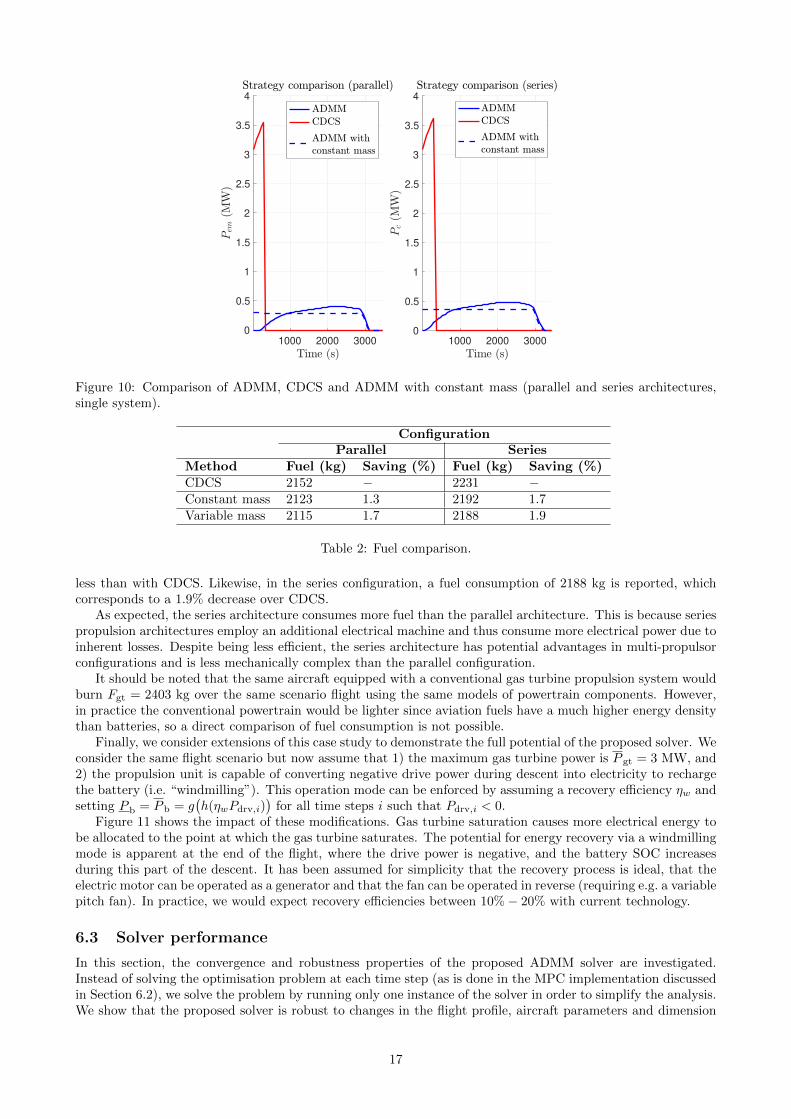
The distribution of the electrical power over time is also illustrated in Fig. 10 in comparison with otherenergy management strategies. The charge-depleting-charge-sustaining (CDCS) strategy is a heuristic that usesall the electrical energy at the beginning of the flight until the battery is depleted and then relies solely on the gasturbine for the remainder of the flight. Interestingly, the proposed ADMM-based approach is the antithesis ofthis strategy, allocating a non-negligible part of the electrical power at the end of the flight. The third strategyillustrated in Fig. 10 uses the ADMM algorithm but ignores the aircraft mass variation. Interestingly, this(necessarily suboptimal) solution distributes the electrical power uniformly over the duration of the flight. Inthis case the strategy is dominated by the need to reduce electrical losses; neglecting the aircraft mass variationmeans that the potential savings due to fuel burn early in the flight are not exploited.

The superiority of the presented variable mass ADMM solver over other strategies is shown in Table 2.The heuristic CDCS strategy is used as a benchmark case. It is shown that the fuel savings with the mass-varying ADMM solver are superior to other strategies, in both parallel and series configuration. In the parallelconfiguration, the proposed energy management strategy achieves a fuel consumption of 2115 kg, namely 1.7%

14

1000 2000 3000

0

1

2

3

500 1000 1500 2000 2500 3000

0

0.2

0.4

0.6

0.8

1

1000 2000 3000

0

1

2

3

500 1000 1500 2000 2500 3000

500

625

750

875

1000

1000 2000 3000

200

400

600

800

1000

1200

1400

Figure 6: Closed-loop ADMM solution to the energy management problem in the parallel and series configura-tions, shown for 1 system (4 overall).

0 1000 2000 3000

400

600

800

1000

1200

1400

1600

0 1000 2000 3000

400

500

600

700

800

900

1000

1100

Figure 7: Comparison of battery and fuel consumption in the parallel and series configurations, shown for asingle system.

15

500 1000 1500 2000 2500 3000

0

0.2

0.4

0.6

0.8

500 1000 1500 2000 2500 3000

0

0.2

0.4

0.6

0.8

1

Figure 8: Effect of changing fuel map coefficient β0 (single system).

500 1000 1500 2000 2500 3000

0

0.2

0.4

0.6

0.8

500 1000 1500 2000 2500 3000 3500

0

0.2

0.4

0.6

0.8

Figure 9: Effect of changing battery resistance R (single system).

16

1000 2000 3000

0

0.5

1

1.5

2

2.5

3

3.5

4

1000 2000 3000

0

0.5

1

1.5

2

2.5

3

3.5

4

Figure 10: Comparison of ADMM, CDCS and ADMM with constant mass (parallel and series architectures,single system).

ConfigurationParallel Series

Method Fuel (kg) Saving (%) Fuel (kg) Saving (%)CDCS 2152 − 2231 −Constant mass 2123 1.3 2192 1.7Variable mass 2115 1.7 2188 1.9

Table 2: Fuel comparison.

less than with CDCS. Likewise, in the series configuration, a fuel consumption of 2188 kg is reported, whichcorresponds to a 1.9% decrease over CDCS.

As expected, the series architecture consumes more fuel than the parallel architecture. This is because seriespropulsion architectures employ an additional electrical machine and thus consume more electrical power due toinherent losses. Despite being less efficient, the series architecture has potential advantages in multi-propulsorconfigurations and is less mechanically complex than the parallel configuration.

It should be noted that the same aircraft equipped with a conventional gas turbine propulsion system wouldburn Fgt = 2403 kg over the same scenario flight using the same models of powertrain components. However,in practice the conventional powertrain would be lighter since aviation fuels have a much higher energy densitythan batteries, so a direct comparison of fuel consumption is not possible.

Finally, we consider extensions of this case study to demonstrate the full potential of the proposed solver. Weconsider the same flight scenario but now assume that 1) the maximum gas turbine power is P gt = 3 MW, and2) the propulsion unit is capable of converting negative drive power during descent into electricity to rechargethe battery (i.e. “windmilling”). This operation mode can be enforced by assuming a recovery efficiency ηw andsetting P b = P b = g

(h(ηwPdrv,i)

)for all time steps i such that Pdrv,i < 0.

Figure 11 shows the impact of these modifications. Gas turbine saturation causes more electrical energy tobe allocated to the point at which the gas turbine saturates. The potential for energy recovery via a windmillingmode is apparent at the end of the flight, where the drive power is negative, and the battery SOC increasesduring this part of the descent. It has been assumed for simplicity that the recovery process is ideal, that theelectric motor can be operated as a generator and that the fan can be operated in reverse (requiring e.g. a variablepitch fan). In practice, we would expect recovery efficiencies between 10%− 20% with current technology.

6.3 Solver performance

In this section, the convergence and robustness properties of the proposed ADMM solver are investigated.Instead of solving the optimisation problem at each time step (as is done in the MPC implementation discussedin Section 6.2), we solve the problem by running only one instance of the solver in order to simplify the analysis.We show that the proposed solver is robust to changes in the flight profile, aircraft parameters and dimension

17

0 1000 2000 3000

-1

0

1

2

3

4

0 1000 2000 3000

400

600

800

1000

1200

1400

1600

0 1000 2000 3000

400

500

600

700

800

900

1000

1100

0 1000 2000 3000

-1

0

1

2

3

4

0 1000 2000 3000

400

600

800

1000

1200

1400

1600

0 1000 2000 3000

400

500

600

700

800

900

1000

1100

Figure 11: Effect of windmilling and gas turbine saturation (single system).

of the problem. Moreover, for conciseness we restrict the analysis to the parallel configuration, all results beingqualitatively equivalent for the series configuration.

Section 6.2 assumed fixed values for the parameters influencing convergence of the algorithm (i.e tolerances,sample rate and penalty parameter update frequency). To investigate the effect of changing the tolerances,Fig. 12 shows accuracy relative to the optimal solution (obtained by solving the problem with CVX and compar-ing total fuel consumption), number of iterations to completion, and required computation time as a function ofrelative tolerance εrel. The latter was varied while keeping other parameters constant (with εabs = 0, Fσ = 105,δ = 10s). As expected, accuracy increases as tolerance decreases but at the expense of a larger number ofiterations and a consequent increase in computation.

It is possible to reduce the tolerance without incurring additional computational cost if the ADMM algorithmis augmented with a penalty parameter update scheme as introduced in section 5. This is illustrated in Fig. 13,which was obtained by varying the update frequency 1/Fσ while keeping other parameters constant (withεabs = 0, εrel = 5× 10−5, δ = 10s). The number of iterations required (and consequently the computation time)decreases as the update frequency increases. However, this tends to decrease accuracy with respect to the CVXsolution. The frequency update should thus be selected with care so as not to affect accuracy.

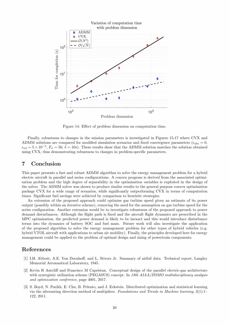
The influence of the sampling interval δ on computation time is shown in Fig. 14 by varying the problemdimension (N = T/δ), with all other parameters kept constant (εabs = 0, εrel = 5×10−5, Fσ = 50). Computationtime increases as problem dimension increases, however, the dependence is O(N2) for CVX and O(

√N) with

the proposed ADMM algorithm. Therefore the proposed solver demonstrates significant computation timedecreases with respect to CVX, allowing longer prediction horizons and real-time convergence.

We further show that a convex formulation of the problem reduces computation significantly compared tosolving the nonconvex problem (15) directly. Retaining only assumption 1) from section 4, the nonconvexproblem is solved using a general purpose nonlinear programming solver (fmincon [27]) with δ = 60 s, achievingconvergence within 82 s. By comparison, under the same conditions, ADMM converges within 0.5 s, showingthe great advantage of the convex formulation3.

3In order to compare the similarity between fmincon and ADMM solutions, a Monte Carlo simulation was conducted by solving100 instances of the problem with battery size randomly sampled from a uniform distribution. The mean absolute error betweenthe solutions (Pb) from both solvers was computed in all 100 scenarios and the variance of the distribution of errors is 9.3 × 10−5

MW2, showing a good agreement between fmincon and ADMM.

18

10-6

10-5

10-4

100

102

10-6

10-5

10-4

0

5

10

104

10-6

10-5

10-4

0

50

100

Figure 12: Effect of varying the relative tolerance on ADMM convergence.

0 0.05 0.1 0.15 0.2 0.25 0.3 0.35

0

200

400

600

800

0 0.05 0.1 0.15 0.2 0.25 0.3 0.35

0

100

200

300

400

Figure 13: Effect of varying the penalty parameters update frequency on ADMM convergence.

19

102

103

100

101

102

Figure 14: Effect of problem dimension on computation time.

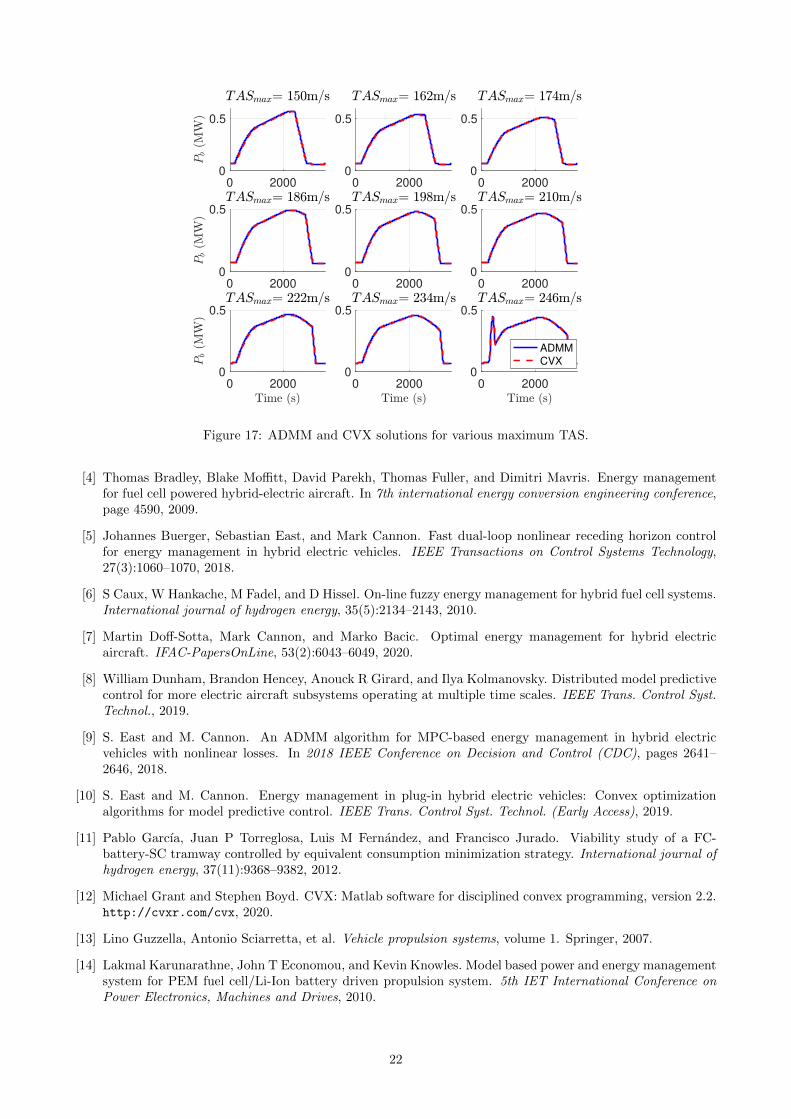
Finally, robustness to changes in the mission parameters is investigated in Figures 15-17 where CVX andADMM solutions are compared for modified simulation scenarios and fixed convergence parameters (εabs = 0,εrel = 5× 10−5, Fσ = 50, δ = 10s). These results show that the ADMM solution matches the solution obtainedusing CVX, thus demonstrating robustness to changes in problem-specific parameters.

7 Conclusion

This paper presents a fast and robust ADMM algorithm to solve the energy management problem for a hybridelectric aircraft in parallel and series configurations. A convex program is derived from the associated optimi-sation problem and the high degree of separability in the optimisation variables is exploited in the design ofthe solver. The ADMM solver was shown to produce similar results to the general purpose convex optimisationpackage CVX for a wide range of scenarios, while significantly outperforming CVX in terms of computationtimes. Significant fuel savings were achieved by comparison to heuristic strategies.

An extension of the proposed approach could optimise gas turbine speed given an estimate of its poweroutput (possibly within an iterative scheme), removing the need for the assumption on gas turbine speed for theseries configuration. Another extension would be to investigate robustness of the proposed approach to powerdemand disturbances. Although the flight path is fixed and the aircraft flight dynamics are prescribed in theMPC optimisation, the predicted power demand is likely to be inexact and this would introduce disturbanceterms into the dynamics of battery SOC and fuel mass. Future work will also investigate the applicationof the proposed algorithm to solve the energy management problem for other types of hybrid vehicles (e.g.hybrid VTOL aircraft with applications to urban air mobility). Finally, the principles developed here for energymanagement could be applied to the problem of optimal design and sizing of powertrain components.

References

[1] I.H. Abbott, A.E. Von Doenhoff, and L. Stivers Jr. Summary of airfoil data. Technical report, LangleyMemorial Aeronautical Laboratory, 1945.

[2] Kevin R Antcliff and Francisco M Capristan. Conceptual design of the parallel electric-gas architecturewith synergistic utilization scheme (PEGASUS) concept. In 18th AIAA/ISSMO multidisciplinary analysisand optimization conference, page 4001, 2017.

[3] S. Boyd, N. Parikh, E. Chu, B. Peleato, and J. Eckstein. Distributed optimization and statistical learningvia the alternating direction method of multipliers. Foundations and Trends in Machine learning, 3(1):1–122, 2011.

20

0 2000

0

0.5

0 2000

0

0.5

0 2000

0

0.5

0 2000

0

0.5

0 2000

0

0.5

0 2000

0

0.5

0 2000

0

0.5

0 2000

0

0.5

0 2000

0

0.5

ADMM

CVX

Figure 15: ADMM and CVX solutions for various battery masses.

0 2000

0

0.5

0 2000

0

0.5

0 2000

0

0.5

0 2000

0

0.5

0 2000

0

0.5

0 2000

0

0.5

0 2000

0

0.5

0 2000

0

0.5

0 2000

0

0.5

ADMM

CVX

Figure 16: ADMM and CVX solutions for various maximum altitudes.

21

0 2000

0

0.5

0 2000

0

0.5

0 2000

0

0.5

0 2000

0

0.5

0 2000

0

0.5

0 2000

0

0.5

0 2000

0

0.5

0 2000

0

0.5

0 2000

0

0.5

ADMM

CVX

Figure 17: ADMM and CVX solutions for various maximum TAS.

[4] Thomas Bradley, Blake Moffitt, David Parekh, Thomas Fuller, and Dimitri Mavris. Energy managementfor fuel cell powered hybrid-electric aircraft. In 7th international energy conversion engineering conference,page 4590, 2009.

[5] Johannes Buerger, Sebastian East, and Mark Cannon. Fast dual-loop nonlinear receding horizon controlfor energy management in hybrid electric vehicles. IEEE Transactions on Control Systems Technology,27(3):1060–1070, 2018.

[6] S Caux, W Hankache, M Fadel, and D Hissel. On-line fuzzy energy management for hybrid fuel cell systems.International journal of hydrogen energy, 35(5):2134–2143, 2010.

[7] Martin Doff-Sotta, Mark Cannon, and Marko Bacic. Optimal energy management for hybrid electricaircraft. IFAC-PapersOnLine, 53(2):6043–6049, 2020.

[8] William Dunham, Brandon Hencey, Anouck R Girard, and Ilya Kolmanovsky. Distributed model predictivecontrol for more electric aircraft subsystems operating at multiple time scales. IEEE Trans. Control Syst.Technol., 2019.

[9] S. East and M. Cannon. An ADMM algorithm for MPC-based energy management in hybrid electricvehicles with nonlinear losses. In 2018 IEEE Conference on Decision and Control (CDC), pages 2641–2646, 2018.

[10] S. East and M. Cannon. Energy management in plug-in hybrid electric vehicles: Convex optimizationalgorithms for model predictive control. IEEE Trans. Control Syst. Technol. (Early Access), 2019.

[11] Pablo Garcıa, Juan P Torreglosa, Luis M Fernandez, and Francisco Jurado. Viability study of a FC-battery-SC tramway controlled by equivalent consumption minimization strategy. International journal ofhydrogen energy, 37(11):9368–9382, 2012.

[12] Michael Grant and Stephen Boyd. CVX: Matlab software for disciplined convex programming, version 2.2.http://cvxr.com/cvx, 2020.

[13] Lino Guzzella, Antonio Sciarretta, et al. Vehicle propulsion systems, volume 1. Springer, 2007.

[14] Lakmal Karunarathne, John T Economou, and Kevin Knowles. Model based power and energy managementsystem for PEM fuel cell/Li-Ion battery driven propulsion system. 5th IET International Conference onPower Electronics, Machines and Drives, 2010.

22

[15] Min-Joong Kim and Huei Peng. Power management and design optimization of fuel cell/battery hybridvehicles. Journal of power sources, 165(2):819–832, 2007.

[16] M Koot, J.T.B.A. Kessels, B. de Jager, W.P.M.H. Heemels, P.P.J van den Bosch, and M. Steinbuch. Energymanagement strategies for vehicular electric power systems. IEEE Transactions on Vehicular Technology,54(3):771–782, 2005.

[17] Wim Lammen and Jos Vankan. Energy optimization of single aisle aircraft with hybrid electric propulsion.In AIAA Scitech 2020 Forum, 2020.

[18] C. Lin, H. Peng, J.W. Grizzle, and J. Kang. Power management strategy for a parallel hybrid electrictruck. IEEE Transactions on Control Systems Technology, 11(6):839–849, 2003.

[19] Wei-Song Lin and Chen-Hong Zheng. Energy management of a fuel cell/ultracapacitor hybrid power systemusing an adaptive optimal-control method. Journal of Power Sources, 196(6):3280–3289, 2011.

[20] Jorge Moreno, Micah E Ortuzar, and Juan W Dixon. Energy-management system for a hybrid electricvehicle, using ultracapacitors and neural networks. IEEE transactions on Industrial Electronics, 53(2),2006.

[21] Pierluigi Pisu and Giorgio Rizzoni. A comparative study of supervisory control strategies for hybrid electricvehicles. IEEE transactions on control systems technology, 15(3):506–518, 2007.

[22] Peter Schmollgruber, David Donjat, Michael Ridel, Italo Cafarelli, Olivier Atinault, Christophe Franccois,and Bernard Paluch. Multidisciplinary design and performance of the ONERA hybrid electric distributedpropulsion concept (DRAGON). In AIAA Scitech 2020 Forum, 2020.

[23] Jinwoo Seok, Ilya Kolmanovsky, and Anouck Girard. Coordinated model predictive control of aircraft gasturbine engine and power system. Journal of Guidance, Control, and Dynamics, 40(10):2538–2555, 2017.

[24] Cosimo Spagnolo, Sharmila Sumsurooah, Christopher Ian Hill, and Serhiy Bozhko. Finite state machinecontrol for aircraft electrical distribution system. The Journal of Engineering, 2018(13):506–511, 2018.

[25] Brian L Stevens, Frank L Lewis, and Eric N Johnson. Aircraft control and simulation: dynamics, controlsdesign, and autonomous systems. John Wiley & Sons, 2015.

[26] Matthias Strack, Gabriel Pinho Chiozzotto, Michael Iwanizki, Martin Plohr, and Martin Kuhn. Conceptualdesign assessment of advanced hybrid electric turboprop aircraft configurations. In 17th AIAA AviationTechnology, Integration, and Operations Conference, page 3068, 2017.

[27] The MathWorks, Inc. Matlab optimization toolbox: fmincon. www.mathworks.com/help/optim/ug/

fmincon.html, 2021.

[28] Jason Welstead and James L Felder. Conceptual design of a single-aisle turboelectric commercial transportwith fuselage boundary layer ingestion. In 54th AIAA Aerospace Sciences Meeting, 2016.

23