Mapping the Human Genome: Current Status

J. C L A I B O R N E S T E P H E N S , * M A R K L . C A V A N A U G H , M A R G A R E T I . GRADIE, M A R T I N L . M A D O R , K E N N E T H K . K I D D

The h u m a n genome has already been the subject o f extensive research activity even though the H u m a n Genome Project is only just officially starting. This review and the accompanying wall chart a t tempt to provide an integrated, quanti tat ive, and detailed summary o f the status o f knowledge on the h u m a n genome in mid-1990. The analysis has lf ighlighted the rudimentary na ture o f many o f the informat ion links needed for the task. While this overview could no t be fully comprehensive and required simplifying assumptions, the results have pro- vided estimates o f relative progress on a region-by-region basis t h roughou t the genome.

A MAP IS A ILEPILESENTATION OF TIlE REIATIOlqSHIPS AMONG

landmarks organized according to a defined coordinate AL ,Iksystem. Genetic maps have been constructed from many different types of data and have used different metrics, from the first genetic linkage map in 1913 (1) to today's detailed molecular maps. Intensified mapping activity over the last decade has generated a substantial amount of data relating to genome organization includ- ing comparisons between organisms (2), functional groups of genes or dispersed gene families, and chromosome regions that have been associated with pathologies (3). The initial phase of the official mapping effort has been focused on the description of order and spatial relationships among genetic landmarks [such as polymor- phisms, genes, and DNA sequences (4)] in order to generate a dense linkage map, a variety of physical maps, and the beginnings of a composite DNA sequence.

Linkage maps. Genetic linkage maps are based on the coinheritance of allele combinations across multiple polymorphic loci. Parental. combinations are usually transmitted if the loci are molecularly close, but recombination at meiosis will generate nonparental combinations more frequently if the loci are farther apart. The primary source of linkage data is the observation of gametic allele combinations. The allelic constitution of gametes for human linkage studies has conventionally been determined indirectly by family studies and statistical inference, but direct molecular analysis of gametes and single chromosomes has recently become possible (5). Whereas distances between loci in kilobases of DNA are additive

J. C. Stephens is in the Laboratory of Viral Carcinogenesis, National Cancer Institute, Frederick, MD, 21701. M. L. Cavanaugh can be contacted through K. K. Kidd. M. I. Gradie is in the Department of Anthropology, Yale University, New Haven, CT 06520. M. L. Mador and K. K. Kidd are in the Department of Human Genetics, Yale University School of Medicine, New Haven, CT 06510. The authors were affiliated with the Yale-Howard Hughes Medical Institute Human Gcoe Mapping Library prior to its closing.

*To whom correspondence should be addressed.

12 OCTOBER 1990

across successive intervals along a chromosome, this is not true for distances measured as recombination frequendes. Therefore, linkage maps use centimorgan units (cM), a measure based on the frequency of recombination, but identical to it only in the limit of small distances (6). A map unit of I cM corresponds, at that limit, to an observation of recombination in 1% of the gametes in the sample (7). The predicted total length for the sex-averaged linkage map is ss00 cM (8).

Physical maps. Physical maps can be cytogenetically or molecularly based. Cytogenetically based physical maps order loci with respect to the visible banding pattem or relative position along the chromo- somes, primarily by means of data from somatic cell hybrids and in situ hybridization (9). Molecularly based physical maps directly characterize large tracts of DNA by establishing molecular land- marks, such as restriction endonuclease sites and sequence tagged sites (STSs) (10). These maps are usually constructed from data generated by pulsed-field gel electrophoresis (PFGE) (1I) or by related techniques that size and order large restriction fragments of genomic DNA. Another molecular strategy is to characterize cloned DNA [in the form of yeast artificial chromosomes (¥ACs) (12), cosmids, or shorter phage vectors] sufficiently to establish overlap- ping assemblages of clones, known as contigs.

Cytogenefic maps have a scale and coordinate system correspond- ing to the chromosome banding pattern. The large-scale restriction maps have a scale on the order of kilobases of DNA (kb) and have not been related to specific chromosome bands. Conversion and comparison between physical maps with such different types of scales is a high priority, but common reference points will have to be mapped and the conversion factors determined empirically. Se- quence-tagged sites have been proposed as the common reference points that could be used to coordinate information from different mapping strategies (10).

The highest level of resolution for a molecularly based physical map is the DNA sequence, which gives the linear order of nudeo- tides for each of the 24 distinct human chromosomes. Leaving aside for the moment the question of sequence polymorphism, a com- plete reference sequence will contain roughly 3 x 109 bp of DNA (13).

The order of loci in physical maps and linkage maps will be the same, but there exists no simple means to convert physical distances into recombination frequencies. Recombination frequencies per megabase of DNA vary considerably by sex and by chromosomal region. The emerging pattern of regional variation shows that telomeric regions have proportionately more recombination in male meiosis and that centromefic regions have higher frequencies of recombination in female meiosis. Overall, there are higher frequen- cies of recombination in female meiosis than male mdosis (usually resulting in longer maps for females), but the ratios of sex-specific map lengths differ among the chromosomes (14).

ARTICLES 237

Short-term (5-year) goals have been established for a few specific types of maps. For physical mapping, the short-term goals are (i) to assemble STS. maps of all human chromosomes with the goal of having markers spaced at approximately lO0,O00-bp intervals, and (ii) to generate overlapping sets of cloned DNA or closely spaced, unambiguously ordered markers with continuity over lengths of 2 x 1 0 6 bp for large parts of the human genome (4).

The short-term goal for the linkage map is to enhance its resolution for each chromosome to a spacing of 2 to 5 cM (4). The >2000 DNA polymorphisms already identified and cataloged would allow construction of a linkage map with average interval size between adjacent loci of about 2 cM. However, published maps have not yet incorporated enough of these to achieve a resolution of more than approximately 5 to 10 cM. Furthermore, since as the distribution of known polymorphic markers is far from uniform, many large gaps will remain until new markers are added.

Quantifying Progress in Human Genome Mapping

The great variability in levels of resolution and the different goals for the various mapping strategies made a single coherent descrip- tion of the progress ofgenome mapping quite challenging. The wall chart in this issue (15) along with the results presented below attempt to provide such a summary. Our objectives were to develop a generally applicable method for quantifying mapping activities on a regional basis throughout the genome and to relate data among different types of maps.

Sources of data. Three primary sources of data were utilized for this study: the Human Gene Mapping Library (HGML) Database (16), the GenBank sequence database (17), and pubfished linkage maps (18-47). The HGML provided the cytogenetic map locations of loci. Broadly defined, a locus may be any genomic location ranging in size from single base pairs to endre gene clusters. For the most part, loci in the HGML are functional genes, pseudogenes, fragile sites, or anonymous pieces of DNA that have been mapped. Probes, on the other hand, are generally cloned pieces of DNA or primer pairs from polymerase chain reaction (PCR) analyses that are used to define or delimit a locus; there are often multiple probes for a given locus. Polymorphisms entered into the HGML are DNA variadous that have been detected primarily by restriction endonu- clease analysis, or more recently by PCR-based analyses. The HGML database included all map locations from the Tenth Interna- tional Human Gene Mapping Workshop (HGM10) and subsequent updates based on articles published or in press through 31 July 1990.

A continuing collaborative effort with GenBank (48) has provided us with the links needed to relate DNA sequence to cytogenetically mapped loci. Most sequence lengths and nucleotide frequencies were current as of GenBank release 64.0.

Preparation of illustrative linkage maps Jbr the wall chart. The knowl- edge necessary for the construction of comprehensive linkage maps is in a state of rapid transition. Few comprehensive linkage maps existed only 4 years ago (49). The CEPH collaboration (50) has had a catalytic effect on this field. There is now the expectation that for most chromosomes consensus maps at better than 10-cM resolution will be published within the next year or two. Many chromosomes already have multiple linkage maps published by different research- ers, but these maps often have few markers in common, making complete integration impossible without additional data. An added complication is the different analytic methods being used to generate maps; multipoint methods simultaneously evaluate several loci while pairwise methods consider loci only two at a time. These different

238

methods involve different assumptions and can yield different results, as noted below. Thus, an attempt at a comprehensive synthesis of the human linkage map is premature. We have instead chosen to present illustrative maps based on the most comprehen- sive oftbe published maps for each chromosome. The maps actually used to prepare these illustrative maps are from the articles noted in Table 1. Many other published linkage studies dealing with smaller numbers of loci exist (51), but were not used in constructing the maps on the wall chart.

The map for each chromosome was prepared by selecting loci m give an average spacing of roughly 10 to 20 cM. The selection of loci was conservative and included only markers with un- ambiguous orders. Markers from separate studies were combined when warranted, but only when no ambiguity of order would be introduced. For example, separate maps of the arms of a chromo- some could be combined if a centromeric locus is shared. Combina- tions largely involved blocks of genes, as for the example above, but occasionally a locus was intercalated into the illustrative map when flanked by markers shared by both maps. In such cases, the flanking markers were far apart and the evidence was compelling that the intercalated marker is between the other two. In choosing which markers to illustrate in the maps, preference was given to genes over anonymous DNA segments, to loci with higher betero- zygosifies, and to loci more frequendy studied. The resulting maps are heuristic in nature and were prepared primarily as a framework to portray the distribufon of polymorphic loci in relation to the linkage intervals.

Genomic coordinate systems. Perhaps the most familiar coordinate system for genomic mapping data is the cytogenetic banding patttem. Conventional summaries (52) of cytogenetic mapping data depict all genes and other loci in relation to the cytological banding patterns of each chromosome, with vertical bars or brackets indicat- ing the interval--encompassing one or more bands--to which a locus has been mapped. The bands are themselves genomic intervals, and can be thought of as the fundamental intervals in the cytogenet- ic coordinate system. Because of overlaps among map locations, cytogenetic summaries become quite cumbersome when a large number of loci are mapped with varying degrees of precision.

Other coordinate systems exist, such as the centimorgan scale for linkage and percentage of chromosome length for in situ hybridiza- tion (53), but conversion among different systems is very difficult, at best. A unifying approach for summarizing the distribution of genes and other mapped loci over different types of maps with diverse coordinate systems would be highly desirable. For all coordinate systems currently in use, the inherent uncertainty in the mapping procedure yields an interval that contains the actual map location, rather than a point. Thus, overlap among map locations are likely to be a continuing problem.

Our solution to this problem was to develop a generally applicable scheme (described below) for quantifying the regional distribution of mapping activity. We have applied the resulting algorithm to the cytogenetic coordinate system. As an approximation to the relative lengths of all chromosome bands, we have used the lengths of the 860 bands (measured at a resolution of 0.1 ram) in the high- resolution International System for Human Cytogenetic Nomencla- ture 1985 (ISCN) depiction (54). The ISCN provides an interna- tionally recognized standard nomenclature and banding pattern with which researchers can unambiguously indicate mapping coor- dinates for a given locus.

Allocation algorithm. Our logic for quantifying mapping activity as a distribution was to break down each map location into its fimdamentai intervals, and allocate each locus proportionally to those intervals. As an example of this procedure, consider a locus mapped to chromosome 1 without regional localization; it has some

SCIENCE, VOL. 250

probability of being in any band on the entire chromosome. On the other hand, a locus mapped to a single band can be said to be in that band with probability = 1, barring mapping errors. Thus, b/Ij is an estimate of the probability that locus j is in band i; where bl is the length of band i,/i is the length of the map location of locus j , and i varies over each band in locus j 's map location. We will take these probabilities as the proportional allocations oflocusj into each band of its map location. When this is done for all mapped loci whose map location includes band i, the total number of loci allocated to band i is

. l j (1)

In this sum bi is a constant, so that the remaining term, Xl//j, is a type of density (loci/length) which, when multiplied by the band's length bi, yields the number of loci allocated to band i. These probabilities are calculated on the basis of the simplifying assump- tion that the only factor determining locus distribution is length of each chromosome band.

Estimating progress towards dosure or completeness. As a working definition, cytogenctic mapping of genes can be considered com- plete when all genes have been identified and have map resolutions of one band. Obviously, this definition does not consider order within bands, but it does allow us to estimate completeness by comparing the number of genes allocated to each band with the number expected to be there.

Let L be the length of the genome, B the number of bands each of

length bi, N the true number of genes, and C the number of mapped genes. Our expectation is that each band contains a number of genes (hi) that is proportional to that band's relative cytogenetic length [nl = N(b/L)] following the same assumption made for the alloca- tion algorithm. Hence, completeness for band i can be calculated as the ratio of current allocation to expectation:

(~2 bi'~ / [b,~ l x J

where, again, the sum is over all genes whose map location includes band i. This is the ratio of gene density within band i to the global gene density (N/L). This rationale can be applied to larger genomic regions, such as individual chromosomes. However, for regions larger than the coordinate system's fundamental intervals, precision of mapping must be taken into account; otherwise, we get trivial estimates such as C/N as an estimate of completeness of gene mapping for the entire genome. The sum Xl//j is an estimate of the total precision for genes mapped to a given genomic region. I f this sum is taken over all C mapped genes, it is an estimate taken over the entire genom¢; if it is taken over the Ct genes mapped to chromo- some k, the sum is an esdmate specific to chromosome k. This sum increases as additional genes are mapped and as map precision increases. At completion, the sums are taken over N and Nk, respectively, in which case we have the approximations

=, = , T {s)

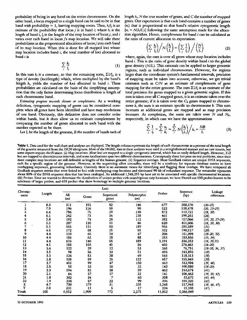
Table 1, Data used for the wall chart and analyses are displayed. The length column represents the length of each chromosome as a percent of the total length of the genome measured from the ISCN ideograms. Most of the HGML data in these analyses were used in a straightforward manner and are raw counts, but some aspects require clarification. (.i) Map locations. Most loci are mapped to a single cytogenefic interval, which has an easily defined length. However, 112 loci are mapped to discontinuous intervals, and some localizadons span two different chromosomes. Conceptually these loci pose no real problems, since their more complex map locations are still definable as lengths of the human genome. (ii) Sequence overlaps. Most GenBank entries are unique DNA sequences, each for a specific region of the genome. However, as the sequencing effort intensifies, there will be a tendency for separate database entries to have overlapping sequences, generating redundancy. Currently there is no automatic means for identi~ing and flagging these overlaps. We have compared all GenBank sequence entries that were linked to loci with overlapping map locations and eliminated 90 kb of redundant sequence. The remainder represents about 80% of the DNA sequence data that has been cataloged. An additional 1,545,255 bp have yet to be associated with specific chromosomal locations. (iii) Probes. Since we wanted to determine the distribution of unique probes with unambiguous map locations, we have filtered out 550 probes known to be subelones of larger probes, and 628 probes that show homology to multiple genomic locations. i F

Loci Chromo- Length Sequenced Polymorphic Probes Sequence Linkage

some All Genes (bp) references loci genes loci

1 8.3 311 192 82 146 677 2 7.9 196 116 50 90 522 3 6.4 786 75 29 130 872 4 6.1 242 73 34 138 461 5 5.8 192 74 28 112 382 6 5.5 207 110 55 86 620 7 5.1 555 121 50 189 965 8 4.5 172 58 25 55 332 9 4.4 110 65 2 4 47 206

10 4.4 156 62 28 88 253 11 4.4 624 140 55 189 1,191 12 4.1 155 103 45 56 402 13 3.6 122 29 1 2 53 265 14 3.5 98 56 33 51 493 15 3.3 126 52 20 49 163 16 2.8 335 59 25 122 457 17 2.7 451 99 47 150 662 18 2.5 55 23 10 32 143 19 2.3 194 82 38 59 462 20 2.1 64 37 17 22 141 21 1.8 202 34 7 60 308 22 1.9 238 57 22 99 396 X 4.7 730 179 31 235 1,245 Y 2.0 231 13 5 17 234

Totals 100 6,552 1,909 772 2,275 11,852

12 O C T O B E R 1 9 9 0

388 576 538 478 112721 199261 157 066 451 606 285 589 190 517 151 098 153 856 336 252 276 461

76 751 243 892 118313 155 443 312,904 100,080 243 674 106 462 32,675

101,325 317 945

15,105 5,066,049

(20-~22) (20, 23-25) (18, 20) (26) (19, 20, 27-29) (18, 20, 30) (31) (20) (18-20, 32) (33, 34) (18, 20,35) (18-2o) (18-20, 36, 37) (18) (38) (2O) (39, 40) (18-20) (41) (19, 20, 42) (43, 44) (45) (18, 46, 47) (#7)

A R T I C L E S 2 3 9

as the expectation for the entire genome, and

• . ~j = . ~ ~- . N b , = L ( 4 )

as the expectation for chromosome k. In the second equation, N, is the number of genes on chromosome k and B, is the number of its bands. The first equality in each equation follows from our assertion that completion is the mapping of every gene to a specific band, and the approximation follows from our assumption that genes are distributed proportionately according to band length. We may now calculate completeness as the ratio

for the entire genome, and

, /6)

for chromosome k. For sequencing, the same logic was applied: we replaced the number of genes allocated to a region with the number of base pairs allocated, and allowed N to be the true number of base pairs in the genome.

Since there is no meaningful limit to the number of probes or polymorphisms in each band, there can be no clear definition of completeness. A contig consisting of overlapping probes that spanned an entire band would constitute completeness for one type of physical map, but a large volume of such data is not yet readily available. Consequently, although we have used color bars to depict gene mapping and sequence completion on the well chart, the color bars for probes and polymorphisms only depict estimates of num- bers per band.

Map location refinement by means of locus order. Most cytogenetic localizations arise directly from physical mapping procedures. How- ever, indirect information such as locus order from linkage maps can be used to verify or refine these localizations. For instance, if three loci are in a known order, the cytogenefic localization of the middle locus is bounded distally by the distal limit of the regional assign- ment for the distal l~us and proximally by the proximal limit of the proximal locus. This logic can be applied sequentially along the chromosome to each locus for which order information is known. The most precisely localized marker will exert considerable con- straint on the regional localizations of a large number of other loci. A clear example is the newly described locus D10S96 (34): the marker only has a chromosomal localization (chromosome 10). Yet, its unambiguous position on the linkage map between DIOS5 and CDC2, both of which are localized to 10q21.1, refines the localiza- tion of D10S96 to lOq21.1.

Since the order of each linkage map limits the possible map refinements, the refinement procedure can be applied iteratively when a collection of maps exists for a single chromosome. When loci are shared among these maps, the shared loci may receive different refinements that can be detected and resolved on each pass. Iteration terminates when there is no further refinement. We have used more than 100 linkage maps containing over 950 distinct loci (55). Two hundred and seventy-four of these loci were selected for illustration in the linkage maps on the wall chart (51). For most chromosomes there were no further refinements after four iterations.

Allocation of polymorphic loci to linkage intervals. The refined localiza- tions were used to portray the number of cataloged polymorphic loci in each interval of the illustrative linkage maps. Polymorphic loci, other than those used in linkage studies, cannot be allocated directly to linkage intervals unless correspondence has been estab- lished between linkage intervals and cytogenetic intervals. The cytogenetic interval corresponding to a specific linkage interval is

240

taken as the union of the refined cytogenetic intervals of the pair of loci determining that linkage interval (56). The sum of polymorphic loci allocated to each band within this cytogenefic interval is our estimate of the number of polymorphic loci within the correspond- ing linkage map interval.

Although each linkage interval is treated independently in this allocation, the fact that adjacent intervals share a common polymor- phic locus means that all polymorphic loci allocated to the cytoge- netic interval of this common locus are counted in both linkage intervals. Because of our refinement procedure, the cytogenetic overlap between adjacent linkage intervals is precisely the cytogenet- ic map location of the shared locus. A consequence of this unavoid- able overlap is that the allocated numbers of polymorphic loci are not additive across the linkage map. They are however, for each single interval, valid maximal estimates.

Analyses of Human Genome Mapping Activity The mapping data used in our overview are summarized in Table

1. Three overlapping subsets of the 6552 loci--genes, sequenced loci, and polymorphic loci--have been analyzed individually because of their relevance to functional characterization, sequencing, and linkage mapping activities, respectively. The allocation algorithm was applied to all loci, genes, sequenced genes, polymorphic loci, probes, and DNA sequence•

In the wall chart, distributions were shown in relation to the chromosome banding pattern. The distributions for genes and mapped DNA sequences were shown as progress towards comple- tion for each band, whereas progress in probe identification was shown as the number of probes within each band. Numbers of polymorphic loci were shown only in relation to the linkage map as described above.

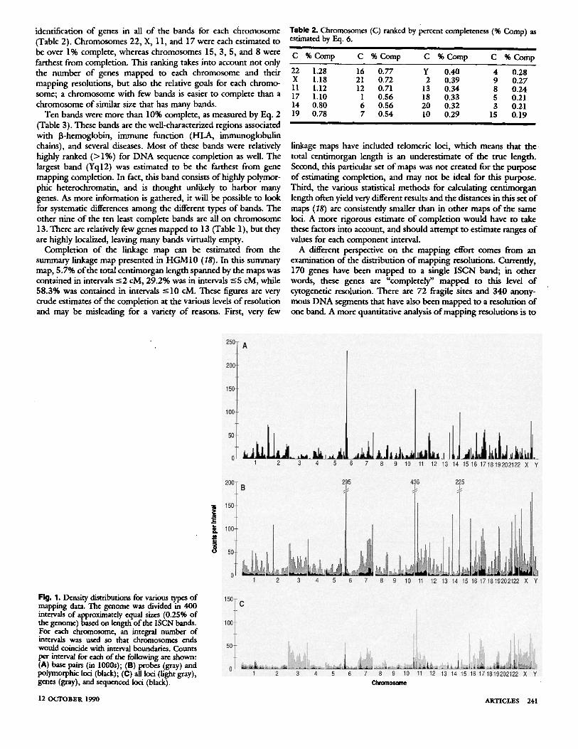
For convenience, each mapping activity has been depicted in Fig. 1 as a histogram with a numeric scale by recasting the results of our allocation to the cytogenetic bands in terms of 400 intervals of roughly equal size. In Fig. 1 polymorphic loci are represented on a cytogenetic length scale, rather than on the centimorgan scale used on the wall chart. In both the wall chart and Fig. 1 the considerable overlap among the various mapping activities is immediately obvi- ous. For instance, localized spikes of activity on chromosomes 6, 11, and 14 (due in part to the HLA cluster, the fl hemoglobin and WAGR regions, and the immunoglobulin heavy chain region, respectively) were found for all types of mapping activity. To quantify this impression, we calculated the correlation coefficient between each pair of mapping activities. All calculated coefficients would have been highly significant i f the distributions of mapping activities were Gaussian. As this does not appear to be the case, variation in magnitude (0.35 to 0.83) could only be used to suggest trends. There was a trend for regions with more sequenced genes to have larger numbers of base pairs allocated. Mapping of all loci and polymorphic loci were positively correlated, but each was poorly correlated with sequenced genes and with base pairs of sequence. The poor association between (polymorphic) loci and sequencing may reflect a preference toward sequencing functional genes. Lastly, the probe distribution was relatively highly associated with all mapping activities, which confirms that probes are central to current mapping strategies.

The genome-wide estimate for complete identification of genes (Eq. 5) was 0.52%. The simple estimate of 1.9% (C/N, where C = 1909 and N = 100,000) was almost fourfold higher, but does not account for mapping resolution. The peaks of activity in Fig. 1 suggest substantial variability in regional progress toward comple- tion. We have used Eq. 6 to estimate progress towards complete

SCIENCE, VOL. 250

i

identification of genes in all o f thc bands for each chromosome (Tablc 2). Chromosomes 22, X, 11, and 17 were each estimated to be over 1% complete, whereas chromosomes 15, 3, 5, and 8 were farthest from completion. This ranking takes into account not only the number of genes mapped to each chromosome and their mapping resolutions, but also the relarivc goals for each chromo- some; a chromosome with few bands is casicr to complete than a chromosome of similar size that has many bands.

Ten bands were more than 10% complcte, as measured by Eq. 2 (Table 3). These bands arc the well-characterized regions associated with [3-hemoglobin, immune function (HLA, immunoglobulin chains), and several diseases. Most of these bands were relatively highly ranked (>1%) for DNA sequcnce completion as well. The largest band (Yq12) was estimatcd to be the farthest from gcne mapping completion. In fact, this band consists o f highly polymor- phic heterochromatin, and is thought unlikely to harbor many genes. As more information is gathered, it will be possible to look for systematic differences among the different types o f bands. The other nine of the ten least compIctc bands are all on chromosome 13. Thcrc arc relativcly few genes mapped to 13 (Tablc 1), but they are highly localized, leaving many bands virtually empty.

Completion of the linkage map can be estimated from the summary linkage map presented in HGM10 (I8). In this summary map, 5.7% of the total centimorgan length spanned by the maps was contained in intervals -<2 cM, 29.2% was in intervals -<5 cM, while 58.3% was contained in intervals -<10 cM. These figures are very crude estimates of the completion at the various levels o f resolution and may be misleading for a variety o f reasons. First, very few

Table 2. Chromosomes (C) ranked by percent completeness (% Comp) as estimated by Eq. 6. H I I l l

C %Comp C %Comp C %Comp C %Comp

22 1.28 16 0.77 Y 0.40 4 0.28 X 1.18 21 0.72 2 0.39 9 0.27 11 1.12 12 0.71 13 0.34 8 0.24 17 1.10 1 0.56 18 0.33 5 0.21 14 0.80 6 0.56 20 0.32 3 0.21 19 0.78 7 0.54 10 0.29 15 0.19

i

linkage maps have included telomeric loci, which means that rthc total cendmorgan length is an underestimate of the truc length. Second, this particular set of maps was not created for the purpose of estimating completion, and may not bc ideal for this purpose. Third, the various statistical methods for calculating ccntimorgan length often yield vcry different results and the distances in this set of maps (18) arc consistently smaller than in other maps of the same loci. A more rigorous estimate of completion would have to take these factors into account, and should attempt to estimate ranges of values for each component interval.

A different perspective on the mapping effort comes from an examination of the distribution of mapping resolutions. Currently, 170 genes havc been mapped to a single ISCN band; in othcr words, these genes arc "completely" mapped to this level of cytogenctic resolution. Thcre arc 72 fragile sites and 340 anony- mous DNA segments that have also been mapped to a resolution of one band. A more quantitative analysis of mapping resolutions is to

Fig. 1. Density distributions for various types of mapping data. The genome was divided in 400 intervals of approximately equal sizes (0.2596 of the genome) based on length of the ISCN bands. For each chromosome, an integral number of intervals was used so that chromosomes ends would coincide with interval boundaries. Counts per interval for each of the following are shown: (A) base pairs (in lO00s); (B) probes (gray) and polymorphic loci (black); (C) all loci (light gray), genes (gray), and sequenced loci (black).

12 OCTOBER 1990

25O- .

20~ °

150"

100-

50-

0 1 2 3 4 5 6 7 8 9 10 11 12 13 14 15 16 171819202122 X Y

2OO B 295 436 225

- 150

0 1 2 3 4 5 6 7 8 9 10 11 12 13 14 15 16 171819202122 X Y

150

100

50

0

C

t 2 3 4 5 6 7 8 9 10 11 12 13 14 15 16 17 1819202122 X Y

Chromosome

ARTICLES 241

100

8O

60

20

0 0.02 0.04 0.06 0.08 Mapping precision

Fig. 2. Cumulative distribution Unctions ofcytogenetic mapping precisions. Mapping precision is measured as percent ofgenome length. Closed squares, all loci; open squares, genes; open diamonds, polymorphic loci; closed diamonds, sequenced genes.

examine the lengths o f all map localizations (Fig. 2). Most loci are mapped to within 1% of the genome; all are mapped to a resolution less than 8.3% (the length of chromosome 1). The average lengths o f map locations are: 1.7% of the genome length for all loci, 1.6% for genes, 1.1% for sequenced genes, and 2.0% for polymorphic loci. Localization of sequenced genes had the highest precision, which suggests that they are generally under intense study. This trend may be bolstered by high-resolution PCR-based mapping techniques that make use of the DNA sequence data. The lower precision of localization o f polymorphic loci reflects the fact that many such loci are anonymous DNA segments that have only been localized by linkage, which typically yields less precise map loca- tions. As loci become more precisely mapped along the chromo- some, the ability to order loci unambiguously will improve, as will the ability to draw relationships between the cytogenetic map and other types of maps such as the linkage map.

Our analyses have only used the chromosomal banding pattern as a coordinate system. In reality, biological differences underlie the observed banding pattern. Many explanations have been proposed, the most common o f which invokes the observed difference in replication timing between light and dark bands (57). Although we cannot test this hypothesis with our data, we can demonstrate how the data can be used to test two other hypotheses. The first is that functional genes tend to be clustered in light bands. I f the bands that cannot be simply categorized as light or dark (for example, centro,

merle bands) are ignored, the genome consists of 413 light bands and 377,dark bands representing 51.2% and 48.8% of the genome length, respectively. When these lengths are treated as the binomial probabilities that a gene falls in a light band versus a dark band, the 99% confidence interval for the propomon o f genes expected in light bands is 48.1 to 54.2%. However, 59.1% (1052.1 of the 1780.7 total genes allocated to light or dark bands) was allocated to light hands, a significant excess. This difference is even more impressive when one considers that the allocation algorithm could obscure this tendency--all genes with map localizations that include multiple bands are allocated proportionally among these bands. A more direct test is to examine genes that have been mapped to a single band. O f the 170 such genes, 115 (68%) were in light bands. Sixty-four of 72 fragile sites (89%) and 266 of 340 anonymous DN A segments (78%) that have been mapped to single bands were also in light bands. Most of the single-copy fraction of the genome is thought to be nonfunctional. Most anonymous DNA segments are single copy and if they are, therefore, nonfunctional, then the perceived clustering o f genes in light bands may be due to systematic mapping biases rather than actual clustering of the genes. Possibili- ties include greater ability to resolve loci within light bands, sampling bias for the loci being mapped (for example, exclusion of repetitive elements or preference for highly expressed genes), or greater condensation of DNA in light bands, and hence more DNA--an explanation contrary to prevailing expectations. Investi- gation of transcriptional activity does not show a bias between light and dark bands (57).

The second hypothesis is that GC content (the percentage of DNA composed of guanine and cytosine base pairs) is higher in light bands than in dark bands (57, 58). The loci that have been sequenced and mapped to single bands provide a relevant data set. The average GC content for sequences linked to loci mapped to a single light band was 0.517; that for sequences linked to loci mapped to a single dark band was 0.507. There was a great amount of variability in the estimates for both band types; GC content for 16 light bands ranged from 0.434 to 0.610, and for 18 dark bands ranged from 0.397 to 0.594. These data suggest no difference in GC content between light bands and dark bands as two classes, but leave open the question o f major differences in GC content among individual bands o f either class. The data used here represent only a fraction of the information that will eventually be available. Im- provements in the resolution o f map locations that have been sequenced and acquisition o f sequencing and mapping data for additional loci will enable researchers to elucidate such basic aspects of genome organization.

Table 3. Individual bands with greater than 10% mapping completeness and the official symbols for selected genes found in each band.

Completion

Band Mapping Sequenc- Representative loci (%) ing (%)

14q32.33 18.3 3.5 IGH@* 12p13.2 15.39 1.74 PRBI, PRB2, PKB3, PKB4 Xp22.32 14.98 0.99 PABX, STS, XG, KAL, CDPX 6p21.31- 12.88 3.1 HLA@*, CYP21, HFE, C2, CAA,

TNFA, TNFB, 17q21.32 12.18 2.22 GP2B, GP3A 22q12.2 10.99 0.12 FRA22B 11p15.5 11.68 2.64 HBB@*, HRAS, MAFDI, INS Xq27.2 10.3 0.08 FRAXD

*@ represents unofficial symbols (as of HGM 10) used for gene clusters, tThe three sub-bands of 6p21.3 share over 70 markers, none of which have been mapped to individual sub-bands.

242

Discussion and Conclusion The methodology developed for this analysis has produced a

multifaceted overview o f current mapping activity and provides a preliminary evaluation of current progress toward mapping the human genome. Through this exercise, some of the limitations of the methodology and the barriers to pre~nting a comprehensive overview inherent in both the data and the manner in which it is recorded have become apparent.

Pertinent data for the human genome project come from a diverse spectrum of disciplines, many of which have immediate goals only incidentally related to gene mapping (for example, medicine, bio- chemistry, physical anthropology, and molecular biology). The compilation and coordination of data from these various disciplines is daunting, and suffers from the lack o f common channels o f communication for the relevant data items. Two major barriers to the expedient integration of data are the lack of a flexible, universal

SCIENCE, VOL. 280

nomenclature, and the variety of mapping resolutions associated with these data items. Even though a rigorous nomenclature exists for genes and mapped segments of DNA (59-61), this nomenclature has only limited usage outside the human gene mapping community and its scope is still too limited to accommodate more general "loci," such as contigs, YACs, and other objects arising in physical map- ping. In addition, official names and symbols are often assigned only after initial publication under very different names. A more general- ized system is needed to allow the broader scientific community easy access to all information on a locus when that information is published in diverse journals under a multiplicity of names. Such a system would facilitate identification of links between different data, such as DNA sequence and map location, which until now have been largely established retrospectively through a laborious manual evaluation of data.

Variability in the level o f resolution of a data item is a very common problem. For example, there are currently several entries for amylase-2 DNA sequences in GenBank; however, the official HGM10 nomenclature recognizes two specific loci, AMY2A and AMY2B. This situation would be partially solved by recognizing these two adjacent genes as a cluster with a single location in the genome, thereby allowing a link between the two types of data. Problems also arise in relating other locus attributes, such as polymorphism, to the individual members of gene clusters. The hierarchical nomenclature needed to resolve such issues for gene clusters is also needed for contigs and their component clones.

To date, efforts to compare maps, even when the links have been clear, have been limited to individual chromosomes or chromosomal regions. Under the rationale that all maps should share the same relative order of loci, we have used locus order as a means for refining cytogenetic map locations across the entire genome. I f used indiscriminately, this method has the potential to propagate errors from one incorrectly but seenlingly precisely positioned locus through the nearby loci. However, as larger numbers of loci are localized with increasing precision, these errors will be detectable as differences in locus order. In an application to one set of linkage maps involving 578 ordered loci (18), only 15 inconsistencies between linkage order and cytogenetic order were found, suggesting that most o f the regional localizations are accurate and consistent with order detived from linkage. The inconsistencies clearly indicate loci and regions requiting additional evaluation. One of the incon- sistencies detected occurred in the middle of the short arm of chromosome 1; it had previously been noted (62). There will inevitably be conflict between maps constructed with different techniques, or even maps constructed independently with the same technique. Clearly, continuous coordination of the different map- ping results is one of the best defenses against mapping errors.

We cannot construct a comprehensive, unified, linkage map at this time. The various published linkage maps for a chromosome often differed considerably in the estimates of distance between loci; in some cases they differed in the order of loci and the sets of loci used in different maps often had minimal overlap. It is not our objective to review these differences in detail, but two points can be made quite strongly. First, different methods of analysis of the same data can give quite different map distances. One example is the map of chromosome 4 where one map (26) based on multipoint mapping methods of primarily CEPH data is almost twice (1.94 times) the length of another map (I8) based on a different method of analyzing essentially the same data. Without discussing the merits o f one analytic approach over the other, it is dear that human map distances are estimates that vary depending on analytic assumptions. The second point is that distance estimates also vary among different data sets because of the inherent sampling error. Compared to the numbers of meiotic products sampled to assemble maps in such

12 OCTOBER 1990

experimental organisms as Drosophila melanogaster, human linkage maps are based on very small numbers, and the distance estimates

h a v e a correspondingly large statistical uncertainty. Our use of the ISCN as a coordinate system, without corrections

for nonuniform distribution o f genes and D N A between chromo- some bands, constrains the interpretation o f our analyses. Band lengths measured from the ISCN (1985) were used became a better coordinate system is not yet available. A molecularly based coordi- nate system could provide the basis for the organization of data from the different mapping activities. F o r example, a map based on physical reference points uniformly spaced every 7.5 Mb would allow generation of histograms with roughly the same resolution as those in Fig. 1. One goal of physical mapping is an STS map with intervals approximately 0.1 Mb in length. Even the smallest cytoge- nefic band is several times larger than this and the average band contains close to 4 Mb; thus, there is a sizable difference in scale between the best molecular resolution represented by cytogenefic coordinates and the objective of an STS map. The estimation and allocation algorithms, and the completeness calculations presented above, could all be cast in terms of intervals defined in an STS map.

The enormity of the task at hand becomes apparent when considering the types of mapping informarion not included in our analyses, yet considered to be crucial to the broader scientific goals of the human genome project. Our analyses have not incorporated information from interspecies comparative maps, nor have we presented (other than as numbers o f identified polymorphic loci) any measure of the kinds of and levels o f normal variation that are expected in human nuclear D N A sequence. Although estimates for the human genome are that 0.3 to 0.5% of base pairs are polymor- phic, no studies representative o f the genome as a whole have yet been undertaken (63). Thus, no global estimate is really justified and region specific estimates need to be empirical.

Ultimately we would like to know the informational content of the genome, and the order and relationship (physical and function- al) among the various regions. The Human Genome Project can be seen as providing the necessary underpinning for this ultimate goal. The impact o f these data should go beyond the immediate concerns of the genome mapping community, allowing scientists in the various fields that have contributed data to answer questions relevant to their own disciplines. This will only be possible if the data are accessible in a form that can readily be utilized by all researchers. With the increase in data generated by mapping efforts, our concept of genome organization will change, with ramifications for a common coordinate system, for nomenclature, and for data- base management. These issues deserve careful consideration, since the way we organize and record data will limit the questions we can pose.

R.EFEI~ENCES AND NOTES I. A. H. Smrtcvanr~ J. Exp. Zool. 14, 43 (1913). 2. S. J. O'Brien, Ed., Cenaic Maps: Locus Maps of Complex Genames (Cold Spring

Harbor Laboratory Press, Cold Spring Harbor, NY, 1990); J. H. Nadea~ Linkage and S~teny Homologies Between Mouse and Man (Jackson Laboratory, Bar Harbor, ME, 1990).

3. V. A. McKusick, Mendelian Inheritance in Man: Catalogs of Autosomal Domimmt, Autosomal Recessive, and X-la'nkd Phenotypes (Johns Hopkins Univ. Press, Balti- more, MD, 1990).

4. U.S. Department of Health and Human Services and U.S. Department of Energy, The U.S. Genome Projea: The First Five Years FY 1991-1995 (National Technical Information Service, Springfield, VA, 1990).

S. H. Li et al., Nature 335, 414 (1988); A. J. ]effreys a al., Cell 60, 473 (1990); G. guano a al., Proc. Natl. Acnd. Sd. U.S.A. 87, 6296 (1990).

6. J. Oth Analysis of Human Genetic Linkage (0ohns Hopkins Univ. Press, Baltimore, MD, 1985).

7. Recombination between any two loci has an upper limit of 50%--independent inheritance--but map distances assembled by adding smaller intervals can reach more than 200 cM for larger chromosomes. See (6) for a discussion of the several mapping functions that relate recombination fraction to map distance.

8. I'4. E. Morton a al., Hum. Genet. 62, 266 (1982). 9. F. H. Kuddlc and Ik. P. Creagan, Aanu. Reu. Gena. 9, 407 (1975); S. I- Goss and

ARTICLES 243

H. Harris, Nature 255, 680 (1975); P. Lichter et al., Doc. Natl. Acad. So'. U.S.A. 85, 9664 (1988).

10. M. Olson, L. Hood, C. Cantor, D. Botsteirg .Science 245, 1434 (1989). 11. D. C. Schwartz and C. K. Cantor, Cell 37, 67 (1984). 12. D. T. Bu.rke; G. F. Carlo, M. V. Olson, Science 236, 806 (1987). 13. National Kesearch Council, Mapping and Sequencing the Human Genome (National

Academy Press, Washington, DC, 1988). 14. J. Wu et al., Am. J. Hum. Genet. 46, 624 (1990); P. O'Connell et al., Genomics 1,

93 (1987); see also (19), (20), and (33). 15. The wall chart enclosed with this issue of Sc/ence, tiffed 'ffhe Human Genome Map

1990' is a graphical representation of many of the ideas presented in this article. Additional copies are available directly from Science.

16. More detailed information about the contents of the HGML can be found in the following papers: J. C. Stephens et al., The Human Gene Mapping Library: Present Status and Future Directions, in Computers and DNA, G. I. Bell and T. G. Marr, Eds. (Addison-Wesley, New York, 1990), p. 69; K. K. Track et al., Banbury Report 32: D N A Technolagy and Forensic Science (Cold Spring Harbor Laboratory Press, Cold Spring Harbor, NY, 1989), p. 335; J. C. Stephens et ~1., The Human Gene Mapping Library: A Resource f ir Studies of Molecular Evolution, Population Genetics, and Comparative Mapping, in Molecular Et, olutiou: UCLA Symposia on Molecular and Cellular Biolagg, , M. T. Clegg and S. J. O'Brien, Eds. (Wiley, New York., 1990), p. 273. The HGML closed permanently on 29 August 1990. The data accumulated in the HGML are available to nonprofit organizations so that they will not be lost to the scientific community. Most specitically, the HGML data became the initial contents of the new Genome DataBase at Johns Hopkins University. Requests for an decuonic copy of the HGML database (more than 50 megabytes) should be directed to K. K. Kidd, Department of Human Genetics, Yale University Medical School, 333 Cedar Sta'~et, New Haven, CT 06510.

17. C. Burks et al., Methods Enz~nol. 183, 3 (1990). 18. B. Keats et al.~ CytaRenet. Cell Genet. 51, 459 (1989). 19. IL White et al., in Genetic Maps: Locus Maps of Complex Genomes, S. J. O'Brien, Ed.

(Cold Spring Harbor Laboratory Press, Cold Spring Harbor, NY, 1990), p. 5.134. 20. H. Donis-Kuller and C. Helms, in ibid., p. 5.158. 21. C. Dracopoli et al., Am. J. Hum. Genet. 43, 462 (1988). 22. P. O'connell et a/., Genomics 4, 12 (1989). 23. S. Povey and C. T. FaIL Cyto~enet. Cell CGenet. 51, 91 (1989). 24. P. O'Couneil et al., Genomics 5, 738 (1989). 25. A. J. Pakstis et al., Cytogenet. Cell Genet. 61, 1057 (1989). 26. D. K. Cox et aL, ibid., p. 121. 27. L. A. Giuffra etal., ibid. 49, 313 (1988). 28. L. A. Giuffra et al., ibid. 51, 1004 (1989). 29. J. L. Kennedy et al., Schizophr. Bull. 15, 383 (1989). 30. H. Blanche et al., Cytogenet. Cell Genet. 51, 963 (1989). 31. G. M. Lathrop et al., Genomics 5, 866 (1989). 32. S. Chambedain et al., CTto~enet. Cell CGenet. 51, 975 (1989). 33. I L L . White et al., Gen0m/cs 6, 393 (1990). 34. J. Wu et al., Genomics, in press. 35. P. Charmley et al., ibid. 6, 316 (1990). 36. J. L. Haines etol., Genet. FEpidemiol. 5, 375 (1988). 37. A. Bowcock et al., Cytogenet. Cell Genet. 51, 966 (1989).

38. Y. Nakamura et al., Genomics 3, 342 (1988). 39. Y. Nakamura et al., ibid. 2, 302 (1988). 40. E. C. Wright et al., ibid. 7, 103 (1990). 41. Y. Nakamura et al., ibid. 3, 67 (1988). 42. M. L. Summar et al., MoL Endocrinol. 4, 947 (1990). 43. R. E. Tanzi et al., Genomio 3, 129 (1988). 44. A. C. Warren et aL, ibid. 4, 579 (1989). 45. G. A. Roulcau et al., ibid., p. 1. 46. F. gouyer et al., Cold Spring Harbor Syrup. Quant. Biol. 51, 221 (1986). 47. D. C. Page et al., Genomics 1, 243 (1987). 48. J. C. Stephens et al., Cytogenet. Cell Genet. 51, 1085 (1989); J. C. Stephens et al., in

preparauon. 49. K. K. Kidd, J. Psychiatr. Res. 21, 551 (1987). 50. J. Dans.set et al., Genomics 6, 575 (1990). 51. A complete list of the linkage maps surveyed is available from the authors. 52. I. H. Cohen et al., in Genetic Maps: Locus Maps of Complex Genomes, S. J. O'Brien,

Ed. (Cold Spring Harbor Laboratory Press, Cold Spring Harbor, NY, 1990). 53. P. Lichter et al., Science 247, 64 (1990). 54. D. G. Harnden and H. P. Klinger, Eds., An Intonational System fir Human

Chromosome Nomenclature (1985): Report of the Standing Committee on Human Cytoge- netic Nomenclature (Karger, New York, 1985).

55. The data used to prepare the illustrative rink, age maps represent only a portion of the maps used in refinement. Presentation of the details of the refinement procedure and resulting refinements for these loci are beyond the scope of this review, and are being prepared for pubfication elsewhere.

56. Strictly speaking, the cytogenetic interval corresponding to the linkage interval is defined by the refined top limit of the upper locus and the refined bottom limit of the lower locus. Although the refinement procedure is not a prerequisite for the allocation of polymorphi¢ loci, our goal was to provide the best possible estimates for the linkage intervals.

57. G. Holmquist et aL, Cell 31, 121 (1982). 58. G. Bernardi et al., Science 228,953 (1985); G. Beruardi, Annu. Rev. Genel. 23, 637

(1989). 59. T. Shows et al., Cytogenet. Cell Genet. 46, 11 (1987). 60. P. McAlpine et al., ibid. 51, 13 (1989). 61. K. Kidd et al., ibid., p. 622. 62. J. Kiddet aL, Genomics 6, 89 (1990). 63. L. Cavalli-Sforza, Am. J. Hum. Genet. 46, 649 (1990). 64. The authors thank L. Manuelidis for in-depth discussions of higher order

chromosome structure, and P. Nadkarni for developing the sequence overlap detection algorithm appfied to GenBank sequences. M. Seashore provided feed- back on the representative genes for the wall chart. B. Jamy provided valuable editorial commentary. H. Cann engaged in many helpful discussions about the linkage maps. The efforts of P. Gfina, M. Skolnick, E. Hildebrand, and M. ConneaUy for their review of the wall chart, are greatly appreciated. We would like to extend a special thanks to the staff of the Yale-HHMI Human Gene Mapping Library: H. Chart, M. Chipperfield, I. Cohen, A. Fenrara, V. Ferriouolo, C. Gawron, S. Knoble, C. Partridge, F. Ricciuti, and R. Track; and to the HGML student assistants A. Boni, C. Boyaiian, A. Dienard, and M. Simmons. Thanks also to W. Alles of the HGM10 workshop staff.

244 SCIENCE, VOL. 250