mapping figures workshop university of utah july 6, 2012 martin flashman professor of mathematics...
TRANSCRIPT
Mapping Figures WorkshopUniversity of Utah
July 6, 2012
Martin Flashman
Mapping Figures WorkshopUniversity of Utah
July 6, 2012
Martin FlashmanProfessor of MathematicsHumboldt State University [email protected]
http://users.humboldt.edu/flashman

Session I Linear Mapping Figures
We begin our introduction to mapping figures by a consideration of linear functions :
“ y = f (x) = mx +b ”
Mapping Figures
A.k.a.Function Diagrams
Dynagraphs
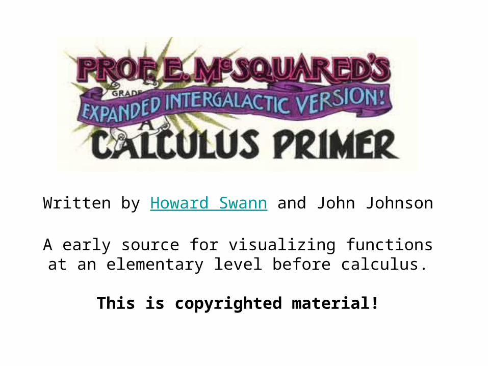
Written by Howard Swann and John Johnson
A early source for visualizing functions at an elementary level before calculus.
This is copyrighted material!


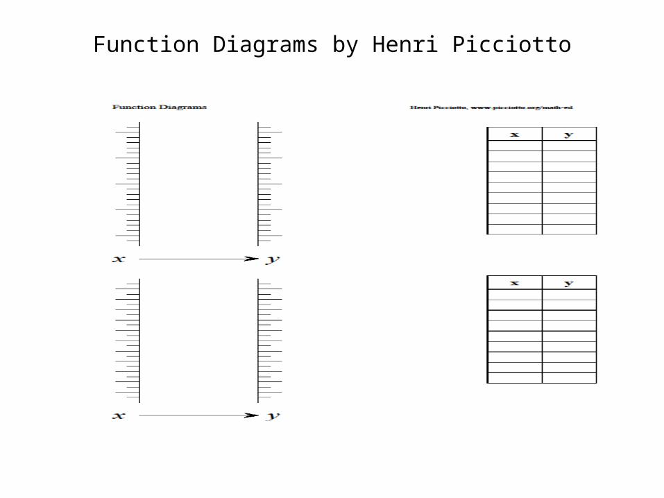
Function Diagrams by Henri Picciotto

a
b
b
a

Mapping Diagrams and Functions
• SparkNotes › Math Study Guides › Algebra II: Functions Traditional treatment.
– http://www.sparknotes.com/math/algebra2/functions/
• Function Diagrams. by Henri PicciottoExcellent Resources!– Henri Picciotto's Math Education Page– Some rights reserved
• Flashman, Yanosko, Kimhttps://www.math.duke.edu//education/prep02/teams/prep-12/

Outline of Remainder of Morning…
• Linear Functions: They are everywhere!
• Tables• Graphs• Mapping Figures• Excel, Winplot and other technology
Examples• Characteristics and Questions• Understanding Linear Functions
Visually.

Visualizing Linear Functions• Linear functions are both necessary, and
understandable- even without considering their graphs.
• There is a sensible way to visualize them using “mapping figures.”
• Examples of important function features (like “slope” and intercepts) will be illustrated with mapping figures.
• Examples of activities for students that engage understanding both function and linearity concepts.
• Examples of these mappings using simple straight edges as well as technology such as Winplot (freeware from Peanut Software), Geogebra, and possibly Mathematica and GSP
• Winplot is available from http://math.exeter.edu/rparris/peanut/

Linear Functions: They are everywhere!
• Where do you find Linear Functions?– At home:
– On the road:
– At the store:
– In Sports/ Games
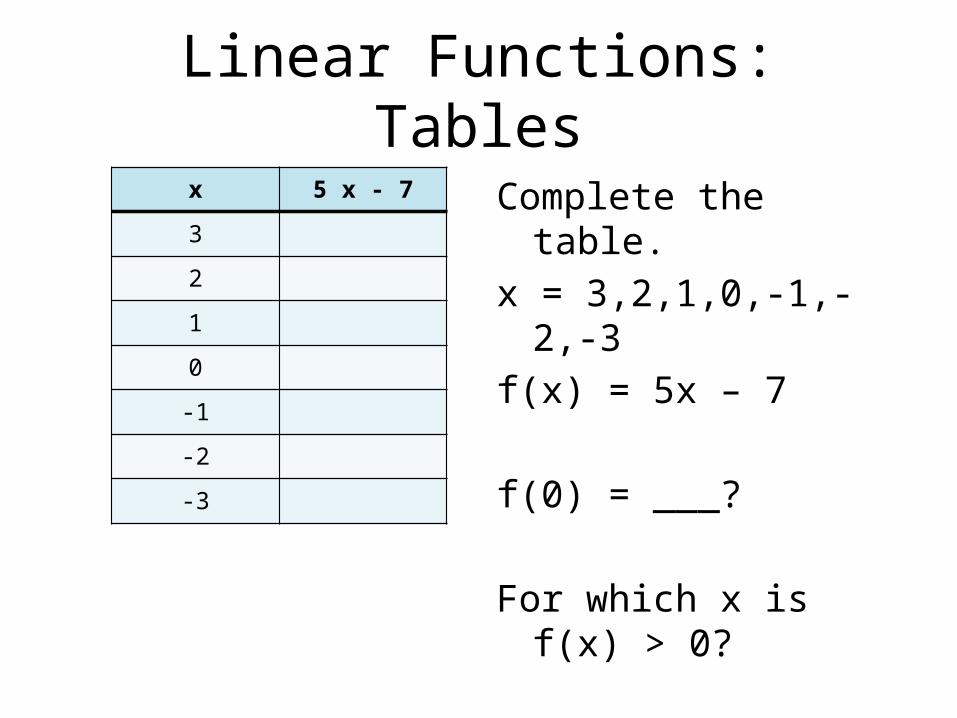
Linear Functions: Tablesx 5 x - 7
3
2
1
0
-1
-2
-3
Complete the table.x = 3,2,1,0,-1,-2,-3f(x) = 5x – 7
f(0) = ___?
For which x is f(x) > 0?

Linear Functions: Tables
x f(x)=5x-73 82 31 -20 -7
-1 -12-2 -17-3 -22
X 5 x – 7
3 8
2 3
1 -2
0 -7
-1 -12
-2 -17
-3 -22
Complete the table.x = 3,2,1,0,-1,-2,-3f(x) = 5x – 7
f(0) = ___?
For which x is f(x) > 0?

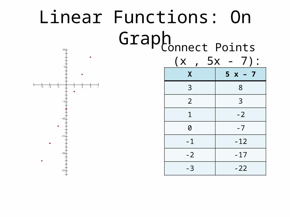
Linear Functions: On GraphPlot Points (x , 5x -
7):
X 5 x – 7
3 8
2 3
1 -2
0 -7
-1 -12
-2 -17
-3 -22
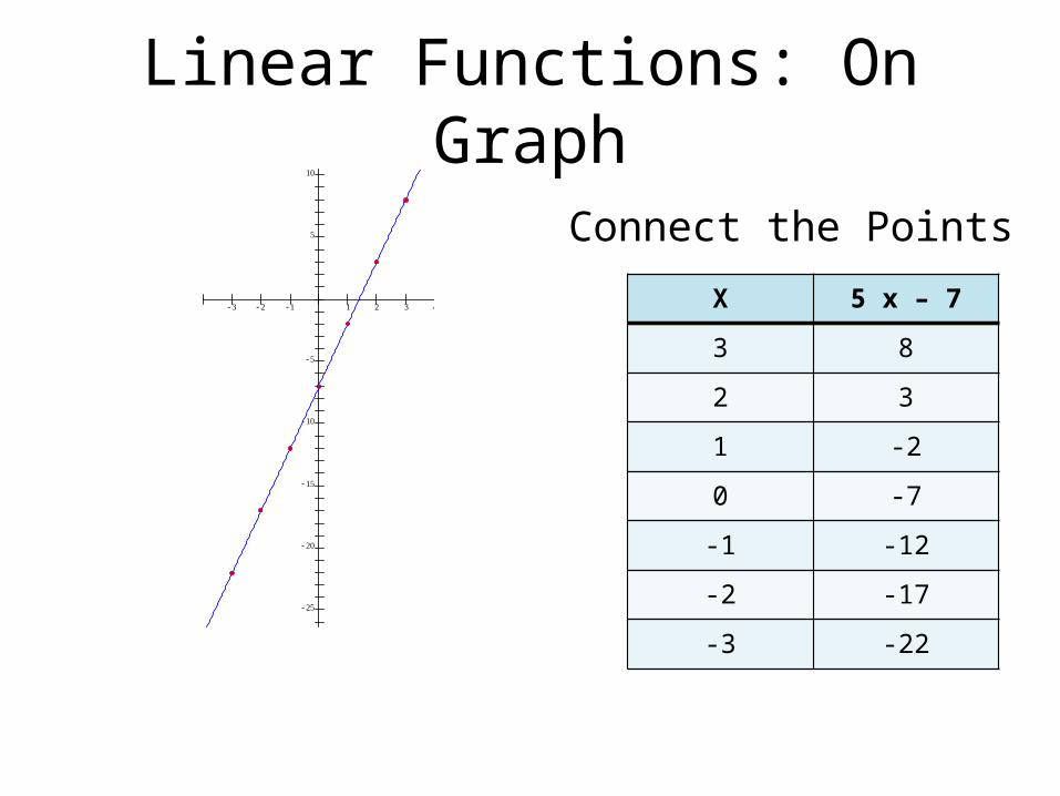
Linear Functions: On GraphConnect Points
(x , 5x - 7):
X 5 x – 7
3 8
2 3
1 -2
0 -7
-1 -12
-2 -17
-3 -22
Linear Functions: On Graph
Connect the Points
X 5 x – 7
3 8
2 3
1 -2
0 -7
-1 -12
-2 -17
-3 -22

Linear Functions: Mapping Figures What happens before the graph.
• Connect point x to point 5x – 7 on axes
X 5 x – 7
3 8
2 3
1 -2
0 -7
-1 -12
-2 -17
-3 -22

-22
-21
-20
-19
-18
-17
-16
-15
-14
-13
-12
-11
-10
-9
-8
-7
-6
-5
-4
-3
-2
-1
0
1
2
3
4
5
6
7
8
X 5 x – 7
3 8
2 3
1 -2
0 -7
-1 -12
-2 -17
-3 -22
Linear Functions: Mapping Figures What happens before the graph.

• Excel example:• Winplot examples:
–Linear Mapping examples• Geogebra examples:
–dynagraphs.ggb –Composition
Examples on Excel, Winplot, Geogebra

Web links• https://www.math.duke.edu//education/prep02/teams/pre
p-12/
• http://users.humboldt.edu/flashman/TFLINX.HTM
• http://www.dynamicgeometry.com/JavaSketchpad/Gallery/Trigonometry_and_Analytic_Geometry/Dynagraphs.html
• http://demonstrations.wolfram.com/Dynagraphs/• http://demonstrations.wolfram.com/ComposingFunctions
UsingDynagraphs/

Function-Equation Questions with mapping figures
• Solving a linear equations: 2x+1 = 5
2x+1 = x + 2 – f(x) = 2x+1: For which x does f(x) =
5 ?– g(x) = x+2: For which x does f(x) =
g(x)?
• Find “fixed points” of f : f(x) = 2x+1 – For which x does f(x) = x?
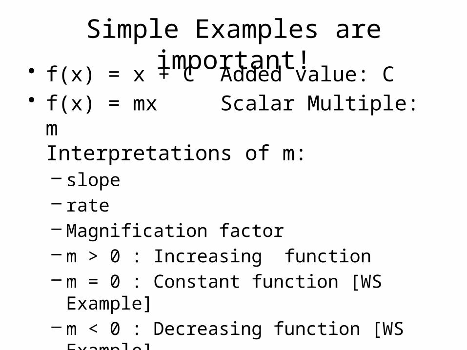
Simple Examples are important!• f(x) = x + C Added value: C
• f(x) = mx Scalar Multiple: mInterpretations of m: – slope – rate – Magnification factor– m > 0 : Increasing function– m = 0 : Constant function [WS Example]– m < 0 : Decreasing function [WS
Example]
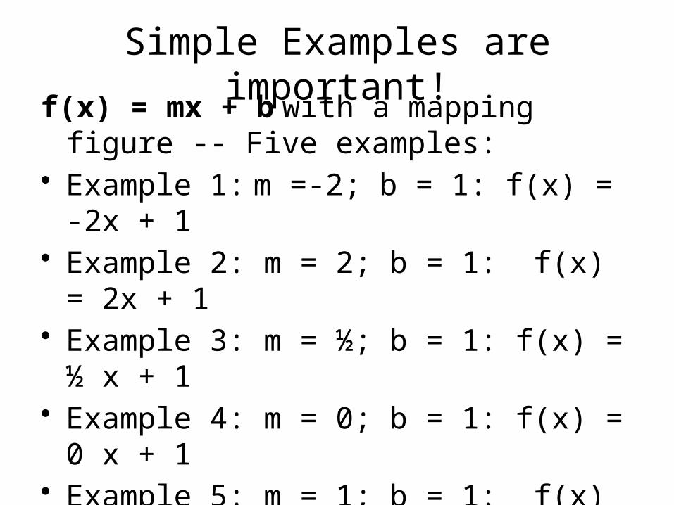
Simple Examples are important!
f(x) = mx + b with a mapping figure -- Five examples:
• Example 1: m =-2; b = 1: f(x) = -2x + 1
• Example 2: m = 2; b = 1: f(x) = 2x + 1
• Example 3: m = ½; b = 1: f(x) = ½ x + 1
• Example 4: m = 0; b = 1: f(x) = 0 x + 1
• Example 5: m = 1; b = 1: f(x) = x + 1
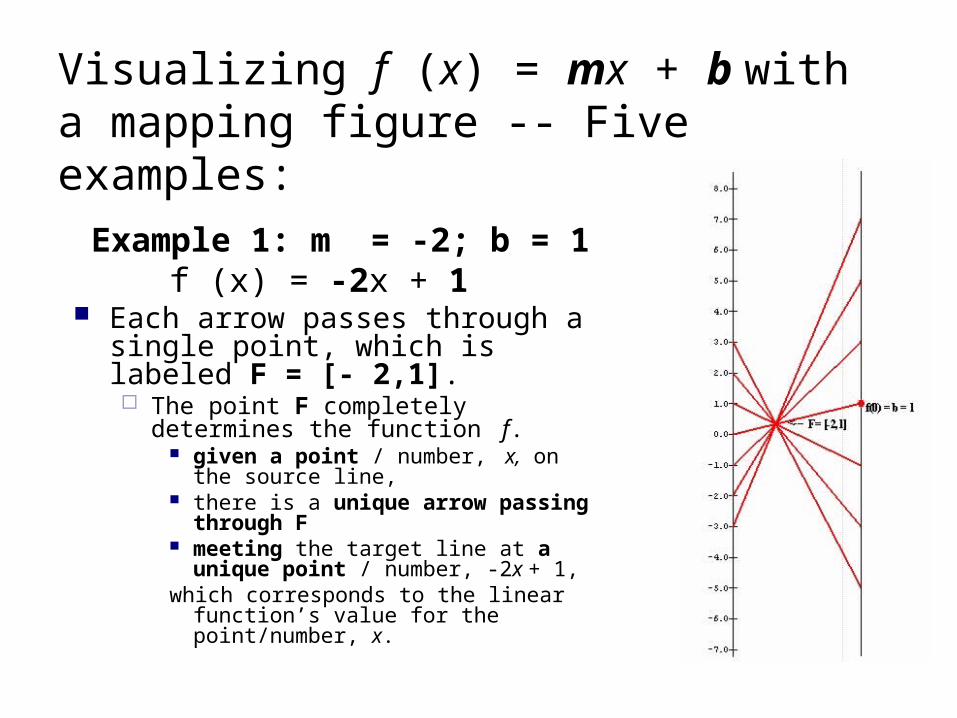
Visualizing f (x) = mx + b with a mapping figure -- Five examples:
Example 1: m = -2; b = 1f (x) = -2x + 1
Each arrow passes through a single point, which is labeled F = [- 2,1]. The point F completely determines
the function f. given a point / number, x, on the
source line, there is a unique arrow passing
through F meeting the target line at a unique
point / number, -2x + 1, which corresponds to the linear
function’s value for the point/number, x.

Visualizing f (x) = mx + b with a mapping figure -- Five examples: Example 2: m = 2; b = 1
f(x) = 2x + 1Each arrow passes through a
single point, which is labeled F = [2,1].
The point F completely determines the function f.
given a point / number, x, on the source line,
there is a unique arrow passing through F
meeting the target line at a unique point / number, 2x + 1,
which corresponds to the linear function’s value for the point/number, x.

Visualizing f (x) = mx + b with a mapping figure -- Five examples: Example 3: m = 1/2; b = 1
f(x) = ½ x + 1 Each arrow passes through a single
point, which is labeled F = [1/2,1]. The point F completely determines the
function f. given a point / number, x, on the
source line, there is a unique arrow passing
through F meeting the target line at a unique
point / number, ½ x + 1, which corresponds to the linear function’s
value for the point/number, x.

Visualizing f (x) = mx + b with a mapping figure -- Five examples:
Example 4: m = 0; b = 1 f(x) = 0 x + 1
Each arrow passes through a single point, which is labeled F = [0,1]. The point F completely determines
the function f. given a point / number, x, on the
source line, there is a unique arrow passing
through F meeting the target line at a unique
point / number, f(x)=1, which corresponds to the linear function’s
value for the point/number, x.

Visualizing f (x) = mx + b with a mapping figure -- Five examples:
Example 5: m = 1; b = 1f (x) = x + 1 Unlike the previous examples, in this case it is not a single point
that determines the mapping figure, but the single arrow from 0 to 1, which we designate as F[1,1]
It can also be shown that this single arrow completely determines the function.Thus, given a point / number, x, on the source line, there is a unique arrow passing through x parallel to F[1,1] meeting the target line a unique point / number, x + 1, which corresponds to the linear function’s value for the point/number, x. The single arrow completely determines the function
f. given a point / number, x, on the source line, there is a unique arrow through x parallel to F[1,1] meeting the target line at a unique point / number, x
+ 1, which corresponds to the linear function’s value for the
point/number, x.

Function-Equation Questions with linear focus points
• Solve a linear equations:2x+1 = 52x+1 = -x + 2 – Use focus to find x.
• “fixed points” : f(x) = x– Use focus to find x.

End of Session I
• Questions• Break - food and thought • Partner/group integration task

Morning Break: Think about These Problems (in Groups 1-2; 3-4)
M.1 How would you use the Linear Focus to find the mapping figure for the function inverse for a linear function when m≠0?
M.2 How does the choice of axis scales affect the position of the linear function focus point and its use in solving equations?
M.3 Describe the visual features of the mapping figure for the quadratic function f (x) = x2. How does this generalize for even functions where f (-x) = f (x)?
M.4 Describe the visual features of the mapping figure for the cubic function f (x) = x3. How does this generalize for odd functions where f (-x) = -f (x)?

Session II More on Linear Mapping Figures
We continue our introduction to mapping figures by a consideration of the composition of linear functions.

Compositions are keys!
An example of composition with mapping figures of simpler (linear) functions.– g(x) = 2x; h(u)=u+1– f(x) = h(g(x)) = h(u)
where u =g(x) =2x– f(x) = (2x) + 1 = 2 x + 1
f (0) = 1 slope = 2
-3.0
-2.0
-1.0
0.0
1.0
2.0
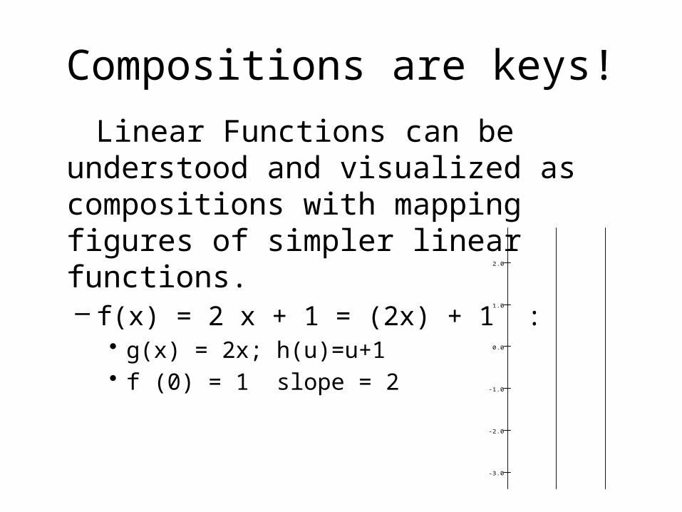
Compositions are keys!
Linear Functions can be understood and visualized as compositions with mapping figures of simpler linear functions.– f(x) = 2 x + 1 = (2x) + 1 :
• g(x) = 2x; h(u)=u+1• f (0) = 1 slope = 2
-3.0
-2.0
-1.0
0.0
1.0
2.0
Compositions are keys!
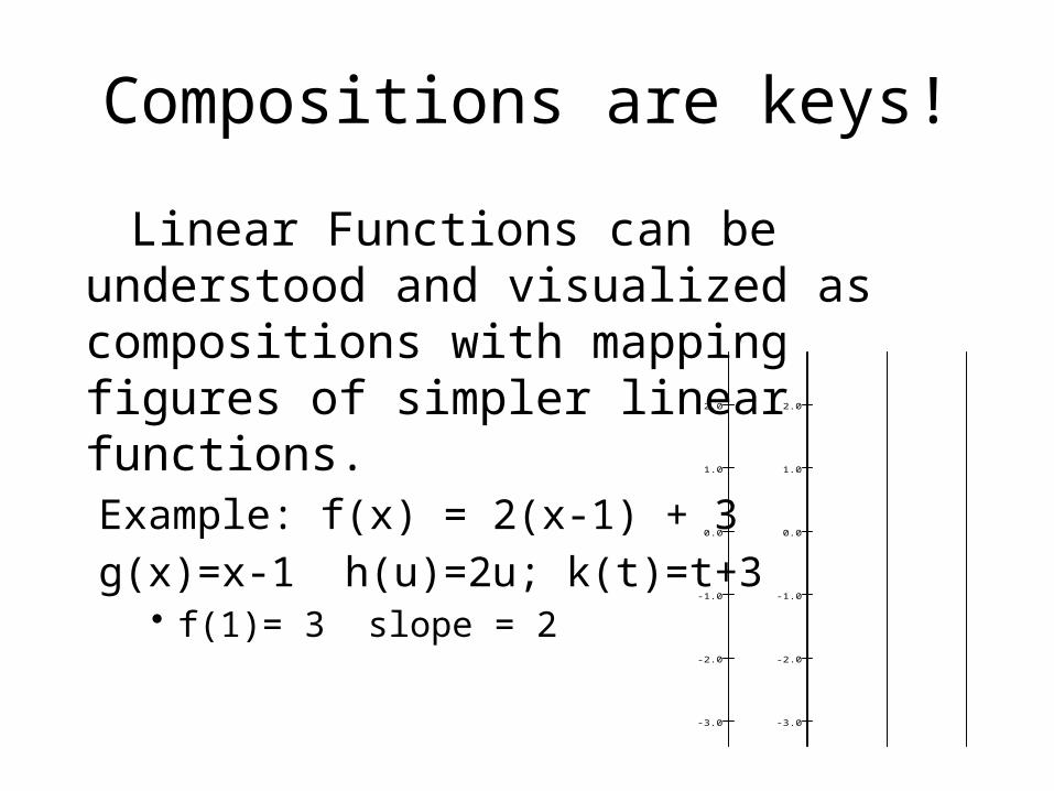
Linear Functions can be understood and visualized as compositions with mapping figures of simpler linear functions.Example: f(x) = 2(x-1) + 3g(x)=x-1 h(u)=2u; k(t)=t+3
• f(1)= 3 slope = 2
-3.0
-2.0
-1.0
0.0
1.0
2.0
-3.0
-2.0
-1.0
0.0
1.0
2.0
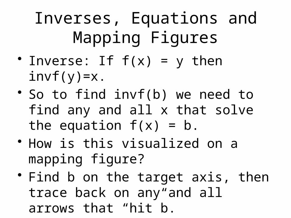
Inverses, Equations and Mapping Figures
• Inverse: If f(x) = y then invf(y)=x.• So to find invf(b) we need to find any
and all x that solve the equation f(x) = b.
• How is this visualized on a mapping figure?
• Find b on the target axis, then trace back on any and all arrows that “hit”b.

Mapping Figures and Inverses
Inverse linear functions: • Use transparency for mapping
figures- – Copy mapping figure of f to
transparency.– Flip the transparency to see mapping figure of inverse function g. (“before or after”)
invg(g(a)) = a; g(invg(b)) = b; • Example i: g(x) = 2x; invg(x) = 1/2 x• Example ii: h(x) = x + 1 ; invh(x) = x
- 1
-3.0
-2.0
-1.0
0.0
1.0
2.0

Mapping Figures and Inverses
Inverse linear functions: • socks and shoes with mapping
figures• g(x) = 2x; invf(x) = 1/2 x• h(x) = x + 1 ; invh(x) = x - 1
• f(x) = 2 x + 1 = (2x) + 1 – g(x) = 2x; h(u)=u+1– inverse of f: invf(x)=invh(invg(x))=1/2(x-
1)
-3.0
-2.0
-1.0
0.0
1.0
2.0
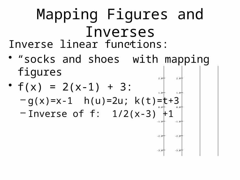
Mapping Figures and InversesInverse linear functions: • “socks and shoes” with mapping figures• f(x) = 2(x-1) + 3:
– g(x)=x-1 h(u)=2u; k(t)=t+3– Inverse of f: 1/2(x-3) +1
-3.0
-2.0
-1.0
0.0
1.0
2.0
-3.0
-2.0
-1.0
0.0
1.0
2.0

End of Session II
• Questions• Lunch Break - food and thought • Partner/group integration task

Lunch Break: Think about These Problems (in Groups 1-3; 4-5)
L.1 Describe the visual features of the mapping figure for the quadratic function f (x) = x2. Domain? Range? Increasing/Decreasing? Max/Min? Concavity? “Infinity”?
L.2 Describe the visual features of the mapping figure for the quadratic function f (x) = A(x-h)2 + k using composition with simple linear functions. Domain? Range? Increasing/Decreasing? Max/Min? Concavity? “Infinity”?
L.3 Describe the visual features of a mapping figure for the square root function g(x) = x and relate them to those of the quadratic f (x) = x2. Domain? Range? Increasing/Decreasing? Max/Min? Concavity? “Infinity”?
L.4 Describe the visual features of the mapping figure for the reciprocal function f (x) = 1/x.
Domain? Range? “Asymptotes” and “infinity”? Function Inverse?
L.5 Describe the visual features of the mapping figure for the linear fractional function f (x) = A/(x-h) + k using composition with simple linear functions.Domain? Range? “Asymptotes” and “infinity”? Function Inverse?

Session III More on Mapping Figures: Quadratic, Exponential
and Logarithmic Functions
We continue our introduction to mapping figures by a consideration of quadratic, exponential and logarithmic functions.

Quadratic Functions
• Usually considered as a key example of the power of analytic geometry- the merger of algebra with geometry.
• The algebra of this study focuses on two distinct representations of of these functions which mapping figures can visualize effectively to illuminate key features.
– f(x) = Ax2 + Bx + C– f(x) = A (x-h)2 + k

Examples• Use compositions to visualize
– f(x) = 2 (x-1)2 = 2x2 -4x + 2
– g(x) = 2 (x-1)2 + 3 = 2x2 -4x + 5
• Observe how even symmetry is transformed.
• These examples illustrate how a mapping figure visualization of composition with linear functions can assist in understanding other functions.

Quadratic Mapping Figures f(x) = 2 (x-1)2 = 2x2 -4x + 2
u = 0.000
y = -2.000
t = 1.000
f(x) = x^2
u = 0.000 y = 0.000x = 1.000
t = 0.000
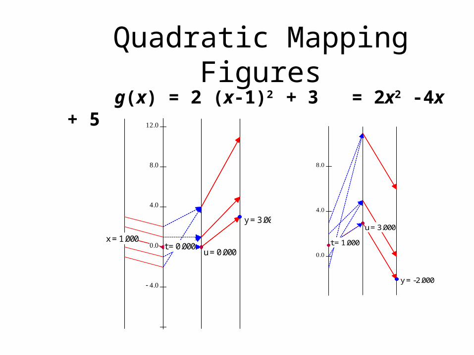
Quadratic Mapping Figuresg(x) = 2 (x-1)2 + 3 = 2x2 -4x + 5
f(x) = x^2
u = 0.000
y = 3.000
x = 1.000t = 0.000
f(x) = x^2
u = 3.000
y = -2.000
t = 1.000

Quadratic Equations and Mapping Figures
• To solve f(x) = Ax2 + Bx + C = 0.• Find 0 on the target axis, then trace
back on any and all arrows that “hit” 0.
• Notice how this connects to x = -B/(2A) for symmetry and the issue of the number of solutions.

Definition
• Algebra DefinitionbL = N if and only if log b(N) = L
• Functions:• f(x)= bx = y; invf(y) = log
b(y) = x
• log b = invf

Mapping figures for exponential functions and
“inverse”
52
x
t
x
t
Visualize Applications with Mapping Figures

“Simple” Applications
I invest $1000 @ 3% compounded continuously. How long must I wait till my investment has a value of $1500?
Solution: A(t) = 1000 e 0.03t. Find t where A(t) = 1500. Visualize this with a mapping figure
before further algebra.

f(x) = 1000*e^(0.03x)
1500
1000

“Simple” Applications
Solution: A(t) = 1000 e 0.03t. Find t where A(t) = 1500. Algebra: Find t where u=0.03t and 1.5
= eu .Consider simpler mapping figure on
next slide

1.5
1

“Simple” Applications
Solution: A(t) = 1000 e 0.03t.
Find t where A(t) = 1500.
Algebra: Find t where u=0.03t and 1.5 = eu .
Consider simpler mapping figure and solve with logarithm:
u=0.03t = ln(1.5) and t = ln(1.5)/0.03 13.52
1.5
1
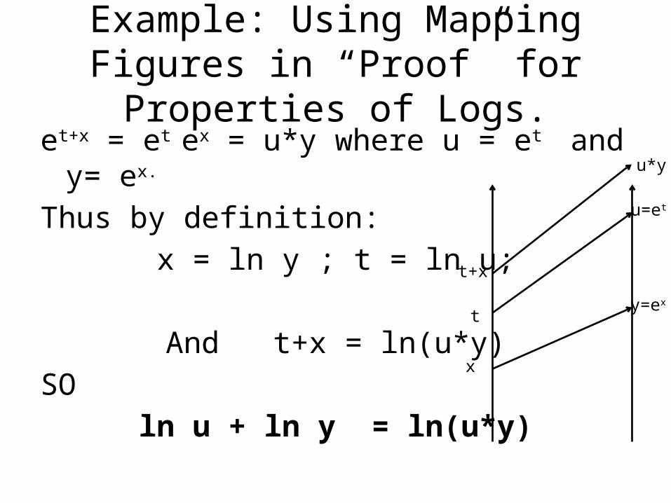
Example: Using Mapping Figures in “Proof” for Properties
of Logs.et+x = et ex = u*y where u = et and y=
ex.
Thus by definition:x = ln y ; t = ln u;
And t+x = ln(u*y)
SO ln u + ln y = ln(u*y)
u=et
y=ex
t+x
x
u*y
t

End of Session III
• Questions• Break - food and thought • Partner/group integration task
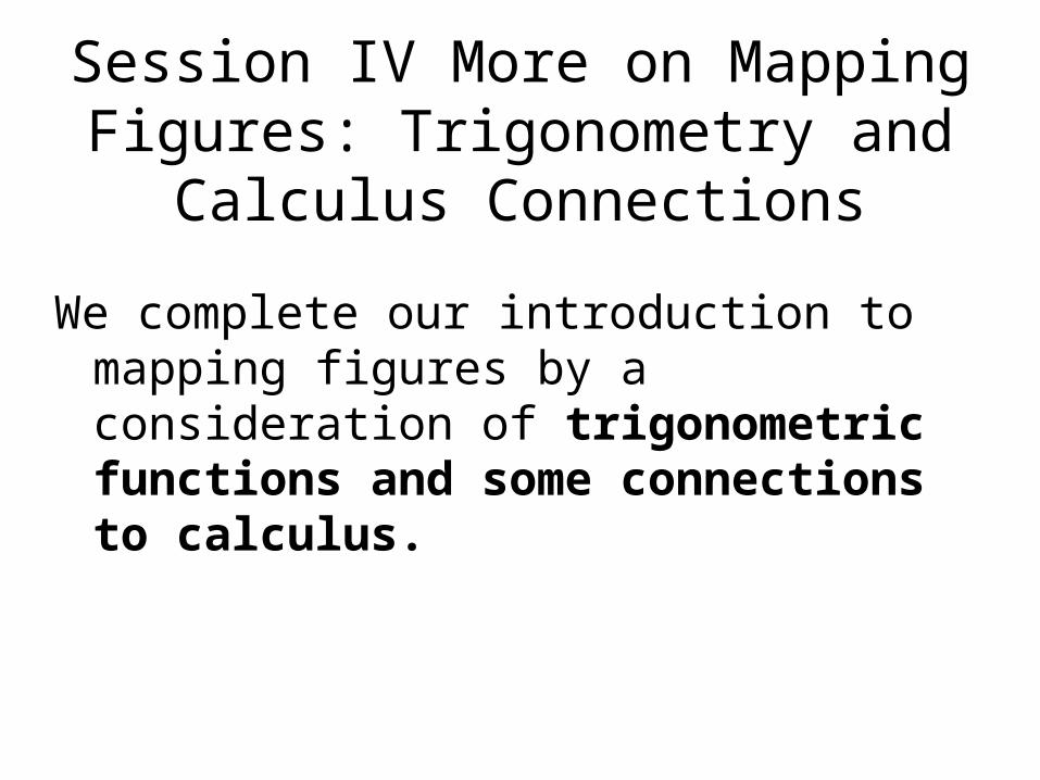
Session IV More on Mapping Figures: Trigonometry and
Calculus Connections
We complete our introduction to mapping figures by a consideration of trigonometric functions and some connections to calculus.
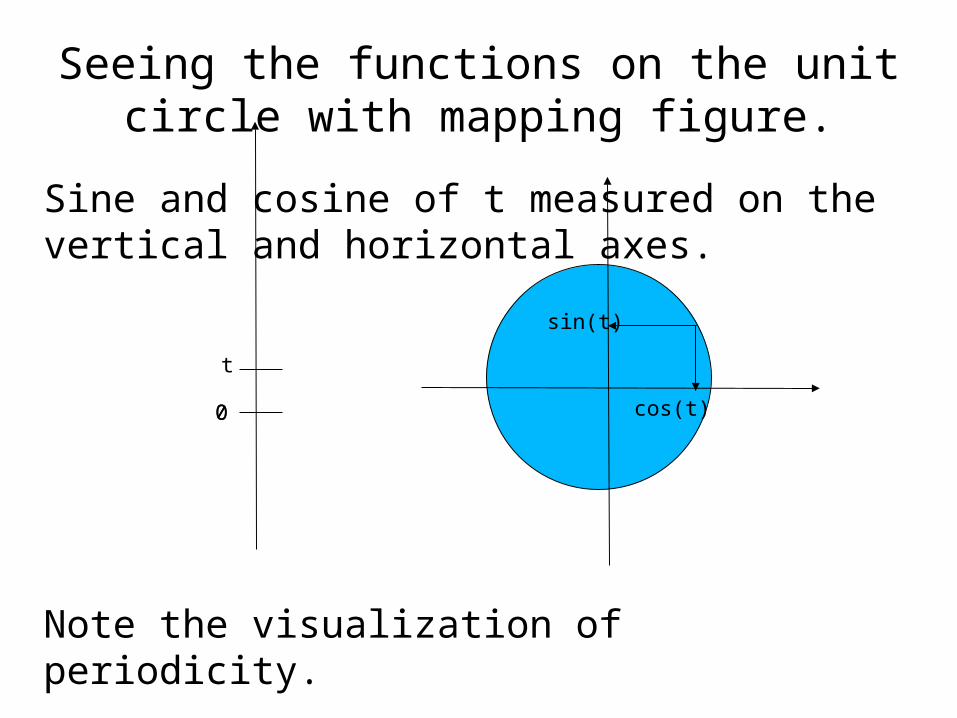
Seeing the functions on the unit circle with mapping figure.
Sine and cosine of t measured on the vertical and horizontal axes.
Note the visualization of periodicity.
00
t
sin(t)
cos(t)

Tangent Interpreted on Unit Circle
• Tan(t) measured on the axis tangent to the unit circle.
• Note the visualization of periodicity.
00
t
(1,tan(t))

Even and odd on Mapping Figures
Even
a f(a) = f(-a)
0
-a
Odd
f(a)
a
0 0
-a
-f(a) = f(-a)
An Even Function
a f(a) = f(-a)
0
-a -a 0 a
f(-a
)= f(
a)
f(a)
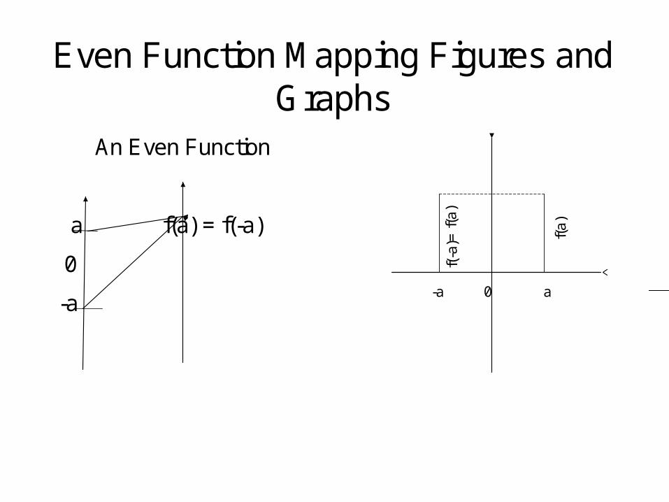
Even Function Mapping Figures and Graphs
An Even Function
a f(a) = f(-a)
0
-a-a 0 a
f(-a
)= f
(a)
f(a
)
• Add graphs here.
66
Odd Function Mapping Figures and Graphs
An Odd Function
f(a)
a
0
-a
f(-a) = -f(a)
-a 0 a
f(-a
)= -
f(a)
f(a)
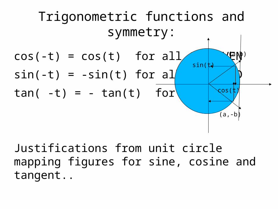
Trigonometric functions and symmetry:
cos(-t) = cos(t) for all t. EVEN
sin(-t) = -sin(t) for all t. ODD
tan( -t) = - tan(t) for all t.
Justifications from unit circle mapping figures for sine, cosine and tangent..
sin(t)
cos(t)
(a,b)
(a,-b)

Trig Equations and Mapping Figures
• To solve trig(x) = z.• Find z on the target axis, then trace
back on any and all arrows that “hit” z.
• Notice how this connects to periodic behavior of the trig functions and the issue of the number of solutions in an interval.
• This also connects to understanding the inverse trig functions.

Solving Simple Trig Equations:
Solve trig(t)=z from unit circle mapping figures for sine, cosine and tangent.
sin(t)=z
cos(t)
Tan(t)=z
Winplot Examples for Trig Functions
Trig Linear Compositions
Compositions with Trig Functions
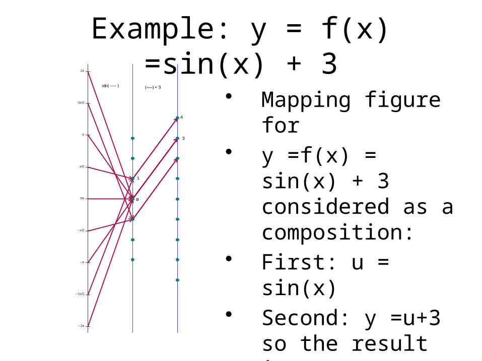
Example: y = f(x) =sin(x) + 3• Mapping figure for • y =f(x) = sin(x) +
3 considered as a composition:
• First: u = sin(x)• Second: y =u+3
so the result is • y = (sin(x)) + 3
sin( ---- ) (----) + 3
0
3
1
4

Example: Graph of y = sin(x) + 3
x
y

Example: y = f(x) = 3 sin(x)
• Mapping figure for
• y =f(x) = 3 sin(x) considered as a composition:
• First: u = sin(x)• Second: y = 3u
so the result is • y = 3 (sin(x))
1
0
s in( ---- ) 3*( ---- )
M ap p ing Figure for y = 3 s in(x) = 3 u w here u = s in(x)

Example: Graph of y = 3 sin(x)
x
y

Interpretations
• y= 3sin(x):
t -> (cos(t), sin(t)) -> (3cos(t),3sin(t))
unit circle magnified to circle of radius 3.
• Y = sin(x) + 3:
t -> (cos(t), sin(t)) -> (cos(t), sin(t)+3)
unit circle shifted up to unit circle with center (0,3).
Show with winplot: circles_sines.wp2;

Scale change before trig.

Scale change before trig.
x
y

Scale change before trig

Altogether!

Mapping figure
sin( ---- ) 3(----) + 2
0
-1
1
5
2
2(----) + pi/3
-pi/6
5pi/6

Graph
x
y
y = 3sin(2x+(pi/3)) + 2


More References

More References
• Goldenberg, Paul, Philip Lewis, and James O'Keefe. "Dynamic Representation and the Development of a Process Understanding of Function." In The Concept of Function: Aspects of Epistemology and Pedagogy, edited by Ed Dubinsky and Guershon Harel, pp. 235–60. MAA Notes no. 25. Washington, D.C.: Mathematical Association of America, 1992.

• http://www.geogebra.org/forum/viewtopic.php?f=2&t=22592&sd=d&start=15
• “Dynagraphs}--helping students visualize function dependency • GeoGebra User Forum
• "degenerated" dynagraph game ("x" and "y" axes are superimposed) in GeoGebra:http://www.uff.br/cdme/c1d/c1d-html/c1d-en.html
More References

