mapping depth to water (dtw) in alberta ... - bera-project.org
TRANSCRIPT

UNIVERSITY OF CALGARY
Mapping Depth to Water (DTW) in Alberta’s Boreal Region Using Remote Sensing Techniques
by
Kirandeep Kaur Basran
A DOCUMENT
SUBMITTED TO THE DEPARTMENT OF GEOGRAPHY
IN PARTIAL FULFILMENT OF THE REQUIREMENTS FOR THE
DEGREE OF MASTER OF GEOGRAPHIC INFORMATION SYSTEMS
GRADUATE PROGRAM IN GEOGRAPHY
CALGARY, ALBERTA
MAY, 2019
© Kirandeep Kaur Basran 2019

Table of Contents
Chapter 1: Introduction ................................................................................................................................ 1
Chapter 2: Literature review ........................................................................................................................ 4
2.1 Remote sensing of groundwater ....................................................................................................... 4
2.1.1 Spectral ........................................................................................................................................ 4
2.1.2 Gravity ....................................................................................................................................... 10
2.1.3 Topographic ............................................................................................................................... 12
2.1.4 InSAR .......................................................................................................................................... 14
2.1.5 Combined gravity and InSAR .................................................................................................... 15
2.1.6 Thermal ...................................................................................................................................... 16
2.1.7 Radar .......................................................................................................................................... 17
2.2 Discussion and Summary ................................................................................................................. 18
Chapter 3: Study Area ................................................................................................................................ 21
3.1 Study area description ..................................................................................................................... 21
Chapter 4: Methods ................................................................................................................................... 23
4.1 Data collection and pre-processing ................................................................................................. 23
4.2 Methodology .................................................................................................................................... 23
4.2.1 Determining continuous GWL and DTW surfaces .................................................................... 24
4.2.2 Generating confidence raster ................................................................................................... 29
Chapter 5: Results ...................................................................................................................................... 33
5.1 GWL and DTW surfaces .................................................................................................................... 33
5.2 Confidence raster surface ................................................................................................................ 35
Chapter 6: Discussion ................................................................................................................................. 39
6.1 Comparison between ‘present study DTW’ and wet areas mapping (WAM) ................................ 42
6.2 Future work ...................................................................................................................................... 45
Chapter 7: Conclusion ................................................................................................................................ 46
References .................................................................................................................................................. 47

List of Figures
Figure 3.1 Study area map (Kirby South) .................................................................................................... 22
Figure 4.1 Workflow for generating continuous GWL and DTW surfaces (Rahman et al., 2017) .............. 25
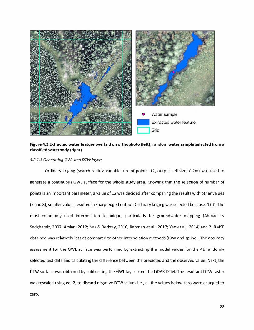
Figure 4.2 Extracted water feature overlaid on orthophoto (left); random water sample selected from a
classified waterbody (right) ........................................................................................................................ 28
Figure 4.3 Workflow for generation of final confidence raster based on four factors .............................. 29
Figure 5.1 Continuous GWL surface obtained through interpolation of random water samples .............. 34
Figure 5.2 Final DTW surface obtained after rescaling ............................................................................... 35
Figure 5.3 Intermediate/Input confidence rasters (slope, ground point density, surface water availability
and wetland probability) ............................................................................................................................. 37
Figure 5.4 Final confidence raster obtained after combining intermediate rasters .................................. 38
Figure 6.1 RGB-NIR orthophoto (left) with zoomed portion of lake (middle) and same area classified as
low wetland probability in the wetland probability layer (right) ............................................................... 39
Figure 6.2 Water feature on RGB-NIR orthophoto (left); same water feature on intermediate ‘quality of
terrain’ confidence raster ........................................................................................................................... 40
Figure 6.3 Orthophoto with water feature (greyish black) (left); classified water feature layer on top of
input slope confidence raster (right) .......................................................................................................... 41
Figure 6.4 Present study DTW values for high confidence areas ............................................................... 44
Figure 6.5 WAM layer for the present study area; with each class signifying the level of wetness .......... 45
List of Tables
Table 4.1 Intermediate confidence rasters and their assigned weights .................................................... 32

Acknowledgements
Firstly, I thank the almighty god, who’s always bestowed upon me many blessings in every phase
of my life. Next, I would like to express my sincere thanks to my supervisor Dr. Greg McDermid, without
whom this research would not have been possible. His continuous faith and motivation encouraged me
to work harder. I can’t thank him enough for all the opportunities he’s got me, for always being available
and providing valuable guidance and suggestion and directing me to the right direction every time.
Throughout the period of my research; Mustafiz and Jen, being both mentor and friend at the same time,
has been an indispensable support to me. A very thank you to all the lab mates (Gus, Silvia, Lucy, Fai and
Annette) for their valuable suggestions, motivation to complete this research and maintaining a friendly
humorous environment in the lab. Thank you to Annette for fulfilling the necessary data needs and
providing the orthophoto, LiDAR point cloud data and DTM. A special thanks to Paulina Medori for always
being considerate.
Most importantly, I want to thank my family, (my mother, father and bestest brother) who has
always been pushing me to reach new heights. Whatever I am today, is the reflection of their efforts and
support.

Abstract
Information on the position of ground water in the boreal forest can assist with our understanding
of ecosystem functioning and provide valuable information for land-use planners. However, traditional
field-based methods are generally suited only to measuring ground-water level (GWL) or depth to water
(DTW) at single points, and are usually used for mapping small areas. The already existing WAM (wet areas
mapping) technique (Murphy et al., 2011) maps large areas but provides static DTW information. Rahman
et al. (2017) developed a workflow for estimating DTW as a space-and-time phenomenon, but the initial
study was carried out over a small and relatively homogeneous study area. In the present study, I apply
extend these techniques over a larger, more-complex study site using surface water as ground-water
predictor. In addition to estimates of GWL and DTW, I also created a confidence raster, based on the
following factors related to our assumptions: a) availability of surface water, b) probability of wetland, c)
quality of the terrain model and d) slope of the terrain. The method works well in wetlands but generates
less confidence in uplands. This method is useful for monitoring DTW over time, in locations that satisfy
our assumptions.

1
Chapter 1: Introduction
Depth to water/water-table (DTW) can be defined as the vertical distance to groundwater table
(GWT) from Earth’s surface. The DTW is related to GWT, except GWT is the height of water table measured
from mean sea level, while DTW is measured from the local surface. An important element of ecosystem
functioning, DTW is the main driver for determining soil-moisture conditions and nutrient availability in
soil (Stumpp & Hose, 2013). Measurements of DTW can contribute to our understanding species-habitat
relationship (Bartels, Caners, Ogilvie, White, & Macdonald, 2018), groundwater ecosystems (Stumpp &
Hose, 2013), plant life cycle, and forecasting flood inundations (Moss, 2016). Several studies have mapped
DTW for estimating soil moisture (Dettmann & Bechtold, 2016; Murphy, Ogilvie, & Arp, 2009; Oltean,
Comeau, & White, 2016), site index (Bjelanovic, Comeau, & White, 2018), variations in soil (Murphy et al.,
2011), and bryophyte assemblages (Bartels et al., 2018) to ultimately understand forest ecosystem
functioning.
Traditional field-based measures of DTW can provide reliable estimates, but are labor-intensive
and generally limited to point measurements (Fitts, 2002). As a result, these techniques are normally used
for mapping small areas and are unsuitable for conducting repetitive measurements through time.
Remote sensing techniques, on the other hand, can complement conventional methods by exploring the
subsurface properties and thus providing an opportunity for conducting repeated DTW estimates over
large and inaccessible areas ( Fitts, 2002; Sibanda, Dube, Seutloali, & Adelabu, 2015).
Since subsurface water is not visible from above, it is difficult to assess directly with remote
sensing. As a result, most studies have relied on indirect or proxy measures such as plant health or
greenness (Koide & Koike, 2012), soil temperature (Heilman & Moore, 1982), or soil moisture conditions
(Pan et al., 2008). Alternatively, several studies have taken advantage of the connection between surface
water, groundwater and topography to estimate depth to groundwater (Caselles, Pitarch, & Caselles,

2
2014; Pfeffer et al., 2014; Rahman, McDermid, Strack, & Lovitt, 2017). For example, Murphy et al. (2011)
integrated LiDAR- (Light Detection and Ranging-) derived DEM (digital elevation model) information with
water features (streams, rivers, wetlands, and lakes etc.) to determine wet areas in Alberta, Canada.
Known as the wet-areas mapping (WAM) approach, the authors began by generating a depression-free
DEM surface using a GIS “FILL” function to create flow direction, flow accumulation and slope gradient
raster surfaces. These surfaces were then used to calculate the elevation difference between a water
feature and other cells in the study area using a least-cost path method (with DTW = 0, for a water
feature). The DTW index thus generated ranged from 0 to 1 with four wetness classes signifying different
levels of associated wetness. The method has been found to work very well in terms of mapping the
annual average DTW, but is somewhat lacking in terms of its usability for mapping instantaneous DTW, or
conducting time-series analysis.
There are certain phenomena that can only be understood well if dynamic DTW information is
available. For instance, determining species (such as, fish assemblages’) response towards fluctuating
water tables (Hebert, 2016; Perkin et al., 2017), quantifying methane emissions (Lovitt et al., 2018),
mapping surface deformations caused due to variations in DTW (Chen et al., 2017), and understanding
relationship between varying DTW and biota (Stumpp & Hose, 2013) etc. For these applications, we would
benefit from alternative techniques to the WAM approach.
Rahman et al. (2017) predicted depth to water using surface water and a digital terrain model
(DTM). Working in boreal wetlands, they first mapped the three-dimensional local of individual water
features using orthophotography and photogrammetric point clouds from a UAV. This same point cloud
was used to make a high-resolution DTM (Lovitt et al., 2017). They used simple interpolation techniques
to approximate the elevation of the water table (measured above sea level) between surface-water
features, then converted this to DTW using the terrain model. While effective, their approach relies on a
number of assumptions. Most importantly, the authors assume that (i) the water table is flat or gently

3
sloping, and (ii) that surface water is tightly connected to groundwater. Rahman et al. (2017)
demonstrated their technique across a 61-hectare wetland near the city of Peace River, Alberta. While
the results were good – root-mean-square errors in the 20-cm range – the study area was small and
without much variability. Also, Rahman et al. (2017) did not produce anything designed to communicate
confidence in the DTW estimates outside of global accuracy statistics.
Considering this, the present study was conducted with the following objectives: 1) to test a
workflow based on Rahman et al. (2017), over a diverse and complex study site, and 2) to generate a
continuous confidence raster surface representing confidence values over varying conditions. I begin first
with a literature review on the use of remote-sensing techniques for mapping groundwater, then proceed
to describing my study which took place in northern Alberta near the town of Conklin.
4
Chapter 2: Literature review
To the best of my knowledge, no review article on the topic of remote sensing of ground water
has been published since 2006 (Becker, 2006). Therefore, the objectives of this chapter are to 1) review
the existing literature on groundwater mapping, particularly water-table position, to provide an outline
of selected methods and findings, and b) to provide suggestions for future research from the gaps
observed in the studies.
2.1 Remote sensing of groundwater
For the purpose of conducting this literature review, the primary database used was “Google
Scholar”. To get an overview of different techniques used in groundwater studies; the following keywords
or similar were searched: “groundwater and remote sensing”, “remote sensing for mapping depth to
water-table”, “groundwater and water-table identification”. The search criteria was then constrained to
individual-level; for instance, “determining water-table position using radar”. Moreover, digging into the
references section of the relevant case studies, review papers, scientific reports helped refining the search
criteria. The present chapter is structured based on the different remote sensing techniques for
groundwater mapping. Each GWL mapping technique- spectral, gravity, topographic, InSAR, combined
gravity and InSAR, thermal and radar has been explained in detail in this section.
2.1.1 Spectral Spectral techniques include interpretation and extraction of information about the object from
the imagery; recorded at different wavelength bands of the electromagnetic spectrum (Meijerink,
Bannert, Batelaan, Lubczynski, & Pointet, 2007). Different objects appear distinct on the satellite imagery
based on their shape, size, location, tone, texture, pattern and height (Tempfli et al., 2009). Previously,
visual interpretation of satellite images was done to discriminate individual hydrogeomorphic units for
prospecting groundwater potential zones (Devi, Srinivasulu, & Raju, 2001; Rai, Tiwari, & Dubey, 2005).
5
The commonly identified hydrogeomorphic parameters were valley fills, floodplains, pediplains, alluvial
plains, ridges, pediments, lineaments etc. (Devi et al., 2001). For example, Gautam (1990) identified buried
channels through visual interpretation of IRS-1A LISS II FCC imagery. Aerial photographs were also visually
interpreted to obtain detailed information about vegetation density, position of leaves, slope etc. He
found that the method successfully identified groundwater as verified by well drilling. Although various
studies reported a positive correlation between hydrogeomorphic parameters and groundwater
occurrence (Agarwal & Mishra, 1992; Devi et al., 2001; Rai et al., 2005); the use of geomorphological units
and lineaments is limited to identify groundwater at shallow and intermediate depths respectively (Devi
et al., 2001).
Another method of groundwater prospecting is the preparation of thematic layers using both
satellite and conventional data, followed by multi-criteria decision analysis (Chowdhury, Jha, Chowdary,
& Mal, 2008; Magesh, Chandrasekar, & Soundranayagam, 2012). For instance, Magesh et al. (2012)
combined IRS-1C satellite data and survey of India (SOI) toposheets to demarcate GWP zones. The
thematic layers were prepared using parameters- drainage density, soil, recharge, lithology, surface water
feature, landform and land slope followed by their weight assignment using the multi-influencing factor
(MIF) technique. This method is again limited to shallow groundwater prospecting (Chowdhury et al.,
2008). Moreover, the reliability of this method is dependent on weight assignment of different thematic
features and thematic layers selection (Chowdhury et al., 2008).
Further use of spectral techniques include the estimation of surface and shallow subsurface
parameters as proxy indicators for mapping GWL. Typically, in arid/semi-arid regions where precipitation
rate is low, shallow groundwater controls soil moisture and is the main source of water to the plant roots
(Pan, Wang, Su, Sun, & Zhang, 2008). The groundwater moves upward to the surface because of the
capillary effect and can be detected by the sensors (Ghulam, Qin, Zhu, & Abdrahman, 2004). The soil
moisture information extraction from spectral imagery is based on the principle that; every material has

6
a unique spectral signature depending upon their different absorption and reflectance properties at
different wavelengths (Sanderson, 2010). For instance, the spectral reflectance decreases with increasing
soil moisture (Ghulam et al., 2004). Based on the concept of soil spectral reflectance, capillary effect;
Ghulam et al. (2004) estimated the groundwater level, for an arid and semi-arid area, using the visible and
infrared regions of Landsat 7 ETM+ imagery. They reported that the soil-moisture in the region was mainly
controlled by groundwater as the chosen study area lacked drainage and irrigation. Moreover, to extract
the soil data alone from the mixed vegetation-soil pixels, a new “optical vegetation cover” method, which
involved weighing the vegetation contribution through a mathematical model, was proposed by them. He
observed a good correspondence between groundwater level distribution and field examinations.
The interconnection between soil moisture, vegetation growth and groundwater has been used
to estimate the depth to groundwater (Komarov et al., 1999; Xiaomei et al., 2007). Pan et al. (2008)
developed shallow groundwater model, for an arid region, by estimating the soil moisture conditions from
MODIS derived normalized difference vegetation index (NDVI) and land surface temperature (LST). The
study was performed on the basis that the region had lower precipitation rates and therefore, surface soil
moisture was related to shallow groundwater. The observations from wells were used to determine the
relationship between depth to groundwater level and soil moisture reflectance. High accuracies were
observed by them for shallow GWL determination using the model proposed. Koide and Koike (2012)
developed a new vegetation index; added green band NDVI (AgbNDVI) using SPOT HRV data
(atmospherically correct), to identify high water table zones based on the differences in the forest trees
conditions. The factors affecting forest trees growth were identified using DEM (Digital Elevation Model),
AgbNDVI values and forest type and the study area was then divided into 555 domains (Koide & Koike,
2012). Based on the histogram of AgbNDVI values, the thresholds for each domain was determined to
extract high vegetation index (VI) points. They found that the high VI points were located on the
groundwater discharge areas when overlaid on the geologic and topographic maps. The borehole
7
investigations from field also verified the high VI points’ accurateness as they were observed to be located
in high water table areas. Additional two new indices- a mean and standard deviation based VI (MSVI), a
revised NDVI (revNDVI) were proposed. The three new indices were compared with the existing VIs (SAVI
(soil adjusted vegetation index), EVI1 (enhanced vegetation index), NDVI, SR); and AgbNDVI was observed
to be superior in terms of water stress sensitivity and differentiating vegetation from other substances.
Ringrose, Vanderpost, and Matheson (1998) determined the depth to groundwater level by
associating the vegetation criteria, identified using field observations, with the thematic mapper (TM)
imagery (geometrically correct). The spatial distribution of “deep rooting species” and “dense woody
cover” was used as indicators of groundwater occurrence. Field identification of deep rooting species was
done to obtain depth. For vegetation/dense woody cover, the water sources and borehole wells were
observed to predict the areas indicative of near surface groundwater. From field observations, 46 woody
cover sites were determined which were associated with the TM imagery afterwards. A geomorphic map,
developed using TM imagery, was used to identify the association between near surface groundwater,
geomorphic subunits and vegetative criteria. The authors found that the dense woody cover was able to
identify sources of near surface groundwater and mapped aquifers in higher areas. Whereas, aquifers in
low-lying areas were identified by deep rooting species. The authors chose the TM imagery for dry season
to avoid mixing of “herbaceous species” and woody cover. They concluded that the vegetation
characteristics can be used as an additional data with other techniques for predicting ground water
locations; with woody cover being more valuable indicator than deep rooting species.
Gramling (2013) identified sediment-filled troughs located between the fractured crust in an arid
region, using conventional hydrologic, geologic, satellite, seismic and gravity data. According to him
troughs are potential groundwater targets and hence were used as groundwater indicator. He developed
a processing strategy called WATEX for processing radar images to remove the obstacles (such as, villages
and rocks) and extract only soil moisture information. He found that five aquifers (each>100m) were
8
identified by WATEX and drilling confirmed the presence of two. Potential evapotranspiration (PET) is
another indicator found in the literature that has been used for estimating the water table depth. As per
Duan, Liu, Wang, and Luo (2015), the temporal patterns in the depth to water table fluctuations are
controlled by precipitation and potential evapotranspiration. The PET is negatively correlated with the
depth to water table (Chen & Hu, 2004). Ndou, Palamuleni, and Ramoelo (2017) attempted to investigate
the applicability of PET as groundwater indicator. The dry season potential evapotranspiration (ETP) was
computed, using SEBAL (Surface Energy Balance Algorithm for Land), by integrating the Landsat images (5
TM; for years 1995 and 2005 and 8 OLI; for 2005) with meteorological data. The relationship between
depth to groundwater level data (obtained from the Department of Water and Sanitation, South Africa)
and ETP was determined using linear regression analysis. The study indicated the applicability of PET as
GWL predictor based on the strong correlation observed between the two; high PET at shallow water
table depth (WTD).
Satellite remote sensing techniques allows the rapid collection of data over large areas; however,
there are concerns associated with the use of satellite data for mapping GWL. The presence of particles
in the atmosphere leads to scattering and absorption of the radiation (Ghulam et al., 2004). Thereby, for
accurate GWL estimation from satellite sensors, calibration of remote sensing data for removing the
atmospheric effects is important (Ghulam et al., 2004). Considering the factors affecting satellite sensors-
coarse resolution and atmospheric interference; Meingast et al. (2014) tested the applicability of earth
observing sensors for detecting water table position. He investigated the relationship between sphagnum
moss and both soil moisture and water table position. The spectral reflectance of sphagnum moss was
estimated using portable spectroradiometer and the measurements were imitated as if they were
obtained from the satellite sensors (MODIS Aqua/Terra, Landsat 8OLI and worldview 2). The moisture
content in vegetation was assessed using narrow band indices (MSI, fWBI980 and fWBI1200) and broad
band indices, derived from earth observing sensors, (SRWI, SIWSI (6,2), ln(Ch5/Ch4) and WV2WI).

9
Comparable results were obtained for narrow band and broad band indices suggesting the usability of
satellite sensors for water table mapping over large areas. Ghulam et al. (2004) corrected the Landsat 7
ETM+ satellite imagery using “6S code” i.e., simulated the satellite signal by considering the constituents
of variable affecting the signal. As a result, the “radiance perturbation” was removed from the Landsat 7
ETM+ imagery (Ghulam et al., 2004). He observed that the GWL was mapped more accurately with the
atmospherically corrected image than the uncorrected Landsat 7 ETM+ imagery; with correlation
coefficients of 0.94 and 0.83 respectively. Moreover, the uncorrected image resulted in wrong GWL
predictions in some areas. An alternative to satellite imagery is the use of high resolution airborne
imagery. An airborne shortwave infrared (SWIR) hyperspectral imagery of 1m spatial resolution, for a 6-
year time-period, was used by Kalacska et al. (2018) to estimate the water table depth in peatland. The
surface moisture was predicted using a narrow band index- normalized difference water index (NDWI).
They found that NDWI successfully predicted the depth to water and thus can be used as water table
depth indicator; because of its sensitivity to both “phenology” and water content present in the
vegetation. The study suggested the consideration of anisotropy property for WTD estimation in peatland
if the image is acquired during summer (leaf on) as soil pixels are interfered with vegetation pixels.
Although various researchers have successfully used proxy indicators- soil moisture, vegetation
characteristics, potential evapotranspiration etc. for GWL mapping; their reliability for groundwater
estimation at greater depths is unsure. The soil moisture is connected to groundwater only up to a certain
depth. No relationship between groundwater and both NDVI and LST was observed for GWD greater than
6m (Pan et al., 2008). Furthermore, the rooting depth and plant type are important factors, as very few
plants have their roots extended to the groundwater (Meinzer, 1927) and each plant has different soil-
water content requirement (Cui & Shao, 2005) respectively. Additional variables such as, vegetation type,
irrigation practices and soil type are important and should be considered (Pan et al., 2008). The pitfall of

10
using PET as groundwater indicator is that irrigated crops and vegetation have similar signatures implying
the impracticality of using PET in that case (Ndou et al., 2017).
2.1.2 Gravity
One of the driving forces behind most of the processes occurring on Earth – gravity – is not same
everywhere. The principle governing gravitational force is its dependence upon mass, with higher masses
pulling the objects with smaller mass towards its center (Lamb, 2009; Rashedi, Nezamabadi-pour, &
Saryazdi, 2009). The minute changes in the earth’s gravity are linked with the continuous redistribution
of water; above and below the surface due to the topographic variations (Liang, Li & Wang, 2012). The
satellite gravity data offered by GRACE- a twin satellite mission, is capable of recording these variations in
the earth’s gravitational field by calculating the changes in velocity and distance between the two
satellites- tracking each other, using microwave radiations (Kerr, 2009). Each satellite’s orbital motion
changes with the changing earth’s gravity; accelerating over strong gravity zones and slowing back down
after the pass (Kerr, 2009).
Typically, the information related to groundwater (such as, volume, groundwater depletion
(GWD) and GWL changes) is obtained by integrating the gravity information with other datasets or
models. The groundwater estimates are then computed by deducting other parameters (for e.g., soil
moisture, lakes and surface water) contributing to hydrology from total water storage (TWS) (Long et al.,
2016; Xiang et al., 2016). For instance, the groundwater irregularities were measured by Swenson,
Famiglietti, Basara, and Wahr (2008) by integrating satellite data from GRACE with soil moisture field
measurements. The difference in the sampled soil moisture observations and the fluctuations in the upper
4m unsaturated zone were computed using a scaling factor, developed from the Department of Energy’s
Atmospheric Radiation Measurement (DOE ARM) network's data. The variations in the groundwater was
estimated using the soil moisture variability difference; and well observations data was used to compare
11
the results. Xiang et al. (2016) integrated satellite gravity data (updated Release-5 GRACE data), satellite
altimetry data and models of both hydrology and glacial isostatic adjustment (GIA), for conducting time-
series (2003 to 2009) analysis of changes in groundwater storage (GWS). The fluctuations in GWS were
determined by subtracting all other components from TWS.
Despite being a global mapping tool, there are issues related to the usability of GRACE data in
relation to groundwater. Discrepancies are observed in the estimates of groundwater changes, possibly
resulting from errors in GRACE or, uncertainties in the models (for e.g., soil moisture model) used to derive
ground water storage (GWS) from the total water storage (TWS) (Xiang et al., 2016). The processing of
GRACE data involves the reduction in noise, leading to signal loss. The restoration of the lost signal is
challenging sometimes, because of human interference and variations in the climate (Long et al., 2016).
Long et al., (2016) stressed the importance of both integrating “a priori information” for improved GRACE
data processing and validation of results with ground observations. The groundwater depletion (GWD)
results as computed by them contradicted estimations from earlier studies. The study argued the
possibility of overestimation of GWD by previous research as they lacked field verification. Another issue
related to GRACE is its coarse spatial resolution (~200,000 km2) making it inapplicable for mapping smaller
regions (Alley & Konikow, 2015; Long et al., 2016). The area should be atleast 200,000 km2 to be mapped
using GRACE satellites (Alley & Konikow, 2015). Furthermore, GRACE being a one-dimensional indicator
of 3D groundwater is incapable of providing information about variations in the groundwater flow (Alley
& Konikow, 2015). To overcome the uncertainties in GRACE data and make it applicable for local-scale
groundwater mapping, Sun (2013) proposed a downscaling approach. An artificial neural network (ANN)
model was developed by combining GRACE-gridded derived gravity data with precipitation and
temperature information (Sun, 2013). The study concluded the feasibility of the method for estimating
GWL changes in the absence of field observations (Sun, 2013).

12
Although the use of GRACE for local-scale mapping is limited, it still provides a big picture of an
area (Alley & Konikow, 2015). The GRACE satellite discontinued in September 2017 and a new GRACE
Follow-On (GFO) mission launched in May 2018 (Frappart & Ramillien, 2018). The coarse resolution issue
of GRACE is expected to be resolved with the launch of GFO (50,000 km2 resolution) (Alley & Konikow,
2015; Frappart & Ramillien, 2018); that has a laser system for determining both velocity and distance
between the coupled satellites (Frappart & Ramillien, 2018). GRACE successfully mapped a variety of
groundwater parameters (for e.g., GWL changes, GWD); however, no evidence for determining the actual
GWL using GRACE satellites was observed in the literature.
2.1.3 Topographic
To a large extent, the movement of groundwater is controlled by topography; flowing from
regions of higher elevation to lower (Fitts, 2002). Moreover, a strong correlation between groundwater
and surface water interactions was determined by Condon and Maxwell (2015). The groundwater and
surface water interactions could be in three ways: - 1) gaining stream- groundwater discharges up into
surface water 2) losing stream- surface water seeps down in different directions to recharge groundwater
3) disconnected stream- there is a gap between the bottom of the surface water and top of the
groundwater (Fitts, 2002; Caselles, Pitarch, & Caselles, 2014; Thomas et al., 1999). For connected stream
(gaining or losing), the surface water and groundwater are in direct contact and therefore, the surface
water (a stream, river or lake) can be regarded as the visible part of groundwater (Caselles et al., 2014).
One of the methods for estimating DTW using a combination of topography and surface water is
to calculate the surface water elevation values followed by GWL estimation based on topography. For
instance, Caselles et al., 2014 predicted the depth to water table of an island, a small and relatively flat
area, using river as groundwater indicator. The topography was determined from ASTER GDEM data and
the DTW was computed from the average of altitude difference between river and each point on the

13
island. A topographical map was used to compare the results followed by validation of values using ten
ground samples. The study concluded the applicability of this method for determining GWL of an area
(island) with same characteristics and size as an RMSE of 1m was obtained. Another study was conducted
by Pfeffer et al., (2014) to determine GWL from surface water elevation assuming that surface water and
groundwater coincides during low water stages i.e., in the absence of seasonal events (rainfall, snow
melt). The ENVISAT altimetry data and SRTM 3” DEM were used to obtain the surface water elevation and
surface topography respectively. Based on topography and gravitational force, the GWL for the whole
study area was determined using natural neighbor interpolation. The results obtained were comparable
with in situ observations.
Another method is the use of topographic-wetness indices as proxies for predicting depth to
water or groundwater level. Rinderer, Van Meerveld, and Seibert (2014) predicted median GWL (or,
shallow GWL) in a steep catchment area with low permeable soils using topographic wetness index (TWI).
LiDAR DTM was used to calculate the topographic parameters- mean curvature, mean slope, TWI, local
curvature, local slope and upslope contributing area. Statistical analysis was performed to determine the
relationship between GWL and topographic variables. According to them, topographic indices can be used
as shallow groundwater predictor in a mountain catchment area as a correlation coefficient greater than
0.6 was obtained. However, they observed a decrease in the correlation between TWI and shallow GWL
during the presence of environmental factors such as rainfall. They also found that the strength of
correlation between the average GWL and TWI depends upon whether the topography is local or upslope
(Rinderer et al., 2014).
These studies indicate that topography and surface water features can be used as groundwater
indicator depending upon the geology of the study area (flat or hill-slope), environmental conditions
(occurrence of rainfall events) and groundwater-surface water interactions. Condon and Maxwell (2015)
in their study observed a strong linear relationship between topography and water table depth for certain

14
areas; this however was not always true for the regions where groundwater fluxes were controlled by
topography. The groundwater and surface water interactions are different during different water periods.
For instance, during high water stages i.e., in the events of rainfall, snow melt, precipitation etc. (Pfeffer
et al., 2014); surface water level rises and might not be used as groundwater indicator. Moreover, the
feasibility of surface water feature as groundwater indicator is restrained by the availability of former in
an area (Rahman et al., 2017).
2.1.4 InSAR
The GWL fluctuations are highly correlated with ground or surface deformations (Ji & Herring,
2012). The pore water pressure increases with increase in the GWL during recharge resulting in expansion
of the surface (Ji & Herring, 2012). On the contrary, the water pressure in the pores decreases with decline
in the GWL during discharge and consequently, the surface contracts (Ji & Herring, 2012). InSAR or
Interferometry SAR can map these deformations or elevation changes in earth’s surface at centimeter or
millimeter-level (Chen, Zebker, & Knight, 2015; Chen et al., 2016) based on the phase difference between
two or more SAR images (Bechor, 2006). Béjar-Pizarro et al. (2017) integrated persistent scatterer
interferometry (PSI) and piezometric data for mapping water table position and variations in the
groundwater storage over a time series of 15 years. The method successfully estimated 80% of the
fluctuations in the GWL. Chen et al., (2017) mapped fluctuations in the groundwater table, to determine
the risk of Angkor monument collapse, using high resolution InSAR (TanDEM-X/TerraSAR) satellite
imageries. They found that the seasonal fluctuations in groundwater could pose a threat for the collapse
of Angkor monument.
Using InSAR in agricultural or forested areas is challenging, as the presence of vegetation can
obscure images, leading to loss of coherence in the phase data (Béjar-Pizarro et al., 2017; Chen et al.,
2016). This might result in uncertainties in the estimates of GWL (Béjar-Pizarro et al., 2017). Béjar-Pizarro

15
et al. (2017) attempted to estimate GWL values in the vegetation affected areas using ordinary kriging
interpolation method. They however, concluded the possibility of unreliable water table values in those
regions. A new automated-algorithm, for processing InSAR data, was proposed by Chen et al. (2015) to
recover the lost deformation information. The L-band ALOS PALSAR data was used to map the
groundwater levels in the agricultural areas (Chen et al., 2016). The method involved the identification of
high quality or stable points having least decorrelation effects i.e., the points not obscured by vegetation;
followed by interpolation to determine GWL for missing areas (Chen et al., 2015; Chen et al., 2016). The
proposed method was successful in reducing the vegetation effects and map groundwater levels at better
spatial and temporal resolution than the conventional existing borehole data (Chen et al., 2016).
The strength of using InSAR for GWL estimation is its capability of covering vast regions (Becker,
2006) and unlike GRACE, InSAR can be used for local-scale mapping because its spatial resolution ranges
between 100 to 5000 km2 (Béjar-Pizarro et al., 2017; Castellazzi, Martel, Galloway, Longuevergne, &
Rivera, 2016). Moreover, it offers highly precise topographic information (Jensen, 2000) and is cost
efficient at the same time (Castellazzi et al., 2016). Older satellites have low temporal coverage which has
been improved by the newly launched satellites- Sentinel-1A, 1B and ALOS-2 (Chen et al., 2016; Castellazzi
et al., 2016).
2.1.5 Combined gravity and InSAR
The individual application of GRACE and InSAR for groundwater mapping has some limitations,
however the combination of these two methods is beneficial (Castellazzi et al., 2016). The groundwater
estimation from GRACE involves the subtraction of all other water components from the total water
storage (TWS) (Castellazzi et al., 2016). Obtaining the information about the other hydrology parameters
(such as, soil moisture) is difficult sometimes (Castellazzi et al., 2016). Moreover, GRACE can’t be used for
downscaling operations due to its low spatial resolution (Alley & Konikow, 2015). InSAR on the other hand

16
supplies the downscaling information but has temporal decorrelation issue; which GRACE doesn’t have
(Castellazzi et al., 2016). Castellazzi et al. (2018) combined GRACE and InSAR to map groundwater
depletion in Central Mexico. The InSAR data was used as an input into the GRACE data to overcome the
latter’s low-resolution limitation. The authors found that the incorporation of InSAR data resulted in
determination of groundwater depletion at higher resolution.
2.1.6 Thermal
The variations in the groundwater depth affects the temperature of the surface parameters
(Huntley, 1978); the soil temperature is low if the water table is shallow (Heilman & Moore, 1982).
Thermal remote sensing technique measures the temperature of the surface objects by recording
electromagnetic radiations in the infrared region (Meijerink et al., 2007). The Heat Capacity Mapping
Mission (HCMM) thermal data was used by Heilman and Moore (1982) for estimating the depth to shallow
groundwater. The correlation between day time thermal image and shallow GWD was observed only
when the vegetation effects were removed (Heilman & Moore, 1982). There is a difference between
groundwater and surface water temperatures (Deitchman & Loheide, 2009). The groundwater
temperature remains constant throughout the whole year, whereas the surface temperature varies on
seasonal cycles (Deitchman & Loheide, 2009; Liu, Liu, Hu, Wang, & Zheng, 2016). Based on this concept,
Deitchman and Loheide (2009) determined water table position at seepage face using ground based
thermal imagery for both summer and winter seasons. The transition between the unsaturated and the
saturated zone was determined based on the temperature differences of surface and groundwater.
Although researchers successfully detected GWD using thermal imagery, it should be noted that
the latter indirectly measures the soil moisture by estimating the temperature of the soil i.e., the wetter
the soil the lower the soil temperature (Heilman & Moore, 1982). Soil moisture is not a suitable indicator
for groundwater estimation at greater depths as the former loses its connectivity to groundwater after a
17
certain depth (Pan et al., 2008). Additionally, the thermal data has temperature information for vegetation
and crops etc., which must be removed before estimating the shallow GWD (Heilman & Moore, 1982).
Moreover, other factors such as, climate, precipitation, evaporation, topography etc. also contribute to
surface temperature variations (Huntley, 1978). According to Huntley (1978) other variables have greater
impact on surface temperature as compared to depth to groundwater and argued that the positive results
by other studies might be due to high evaporation rates linked with increased soil moisture. He concluded
that using thermal infrared data for direct estimation of GWD is impractical as discriminating whether the
surface temperature variations are due to variations in the depth to groundwater or driven by changes in
evaporative rates is difficult.
2.1.7 Radar
Radar, because of its ground penetration capabilities can image subsurface structures (Maheswari
et al., 2013) and is used to determine GWL. The radar principle for water table detection is based on its
sensitivity to changes in the dielectric constant of the material (Trenholm, 2000). A radar wave
propagating inside earth’s surface either reflects or transmits (Manu & Preko, 2014) whenever the
dielectric constant changes, in this case, from unsaturated to saturated conditions (Trenholm, 2000). The
total travel time of the wave- to pass through the surface, reflect off from the water table and return to
antenna; is recorded by the ground penetrating radar (GPR) system (Seger & Nashait, 2011). The depth to
water table is determined from the total travel time and the velocity of signal in the soil (Seger & Nashait,
2011). Studies have been conducted based upon radar concept for determining groundwater level (Manu
& Preko, 2014; Seger & Nashait, 2011). Johnson (1992) mapped water table using GPR and obtained a
success rate of 60%. The comparison between radar derived GWL estimates and well observations
revealed an average difference and standard deviation of 7% and 6.4% respectively.
18
As soil’s conductivity or dielectric constant is dependent upon water volume present; the radar
penetration depth varies with the moisture content (Trenholm, 2000). Moreover, soil type- whether
sediments are present or finely grained soil; also affects the radar signal penetration (Saintenoy &
Hopmans, 2011). Johnson (1992) in his study reported that the penetration depth in clay and clay-free
soils was approximately 3% and 95% respectively. This implies that it is not always possible to detect GWL
using radar as in the case of fine textured or clay soils (Saintenoy & Hopmans, 2011) and thus this
technique is limited to shallow GWL mapping. Additionally, for accurate shallow GWL measurements, it is
important to estimate capillary fringe because of its existence between saturated and unsaturated zones
(Trenholm, 2000).
2.2 Discussion and Summary
The present chapter attempted to explore different methods for determining the water table
position and identify the areas for progress. The hydrogeomorphological features provides useful
information about the occurrence of groundwater. Shallow groundwater can be estimated by visually
interpreting the satellite imagery and identify hydrologic and geomorphic units- buried channels,
pediments, alluvial plains, fractures, lineaments and cracks etc. In arid/semi-arid environments, the
vegetation growth might be influenced majorly by groundwater and the relationship between soil
moisture, plants and groundwater is a useful indicator of groundwater at shallow depths in such cases. A
common practice is to derive soil moisture information either from spectral, thermal or radar imagery to
determine groundwater at shallow depths. The information obtained is sometimes supplemented with
the vegetation growth or plant characteristics data determined usually from spectral imagery. Shallow
groundwater tables have also been predicted using surface temperature. Another approach is to use a
combination of topographic information and surface water elevations, derived from spectral, altimetry,
UAV-DEM and LiDAR-DEM, for mapping GWL. Other than these proxy measures, the direct measurements
of groundwater include the gravity data from GRACE and surface elevation changes measured by InSAR.
19
Both GRACE and InSAR have their individual limitations; however, a combination of both the techniques
is beneficial in mapping groundwater.
Though a wide range of techniques have been used for groundwater-table mapping, there are
certain areas where progress can be made. Based on earlier studies, few suggestions or, future
recommendations have been proposed which are listed below. It has been noted there is no universal
technique for GWL estimation as each technique has its pros and cons for reliably estimating GWL. As
observed in the studies of Béjar-Pizarro et al. (2017) and Rahman et al. (2017) the mapping of groundwater
level in areas covered with dense vegetation is difficult. In such cases, the areas that are missed or that
have unreliable groundwater estimates could be mapped using supplementary data.
This supplementary data could be obtained from any other technique, depending upon the study
area or the problem encountered. For example, proxy measures could be used, and the vegetation or
moisture indices can be derived from spectral data. Alternatively, radar can also be used to determine the
water table position for the areas that are missed. This technique has the benefit of working under all
weather conditions and penetrate ground depending upon soil type. Based on this, various combinations
can be proposed that are listed below: InSAR-spectral, UAV-thermal and so on. It should be noted that
spectral, radar and thermal techniques have their own limitations and are only applicable under certain
conditions/assumptions. Thus, the use of these techniques has only been proposed as a supplementary
data source. They might not provide detailed information but can be used to obtain approximate GWL
values for the affected regions when the technique being used fails. Alternatively, as per Rahman et al.,
(2017) a high point density LiDAR, capable of penetrating canopies, could be used to determine the GWL
values for uplands and densely forested areas.
The above-mentioned suggestions employ the use of proxy measures as an additional data.
Moreover, certain methods found in literature are based on using topography, surface water-
20
groundwater interactions information for estimating GWL. Such methods are dependent upon the
availability of a surface parameter in a particular study area. GRACE and InSAR, capable of providing direct
global estimates of groundwater, are independent of any proxy indicator and are thus applicable in the
absence of a surface groundwater indicator. The combined approach of GRACE and InSAR has been used
for estimating groundwater depletion but its use for depth to water-table determination has not yet been
exploited. The benefit of conducting future studies using combined GRACE and InSAR are: no surface
indicator/parameter are required and depth to water-table can be determined over large areas.
In nutshell, use of just one technique might not provide the desired results, the integrated
approach on the other hand, could prove to be beneficial. The mapping of GWL can be improved by
adopting combined approach strategies as the fusion of two or more techniques can successfully
overcome the individual limitations. The selection of a particular technique however, depends upon the
complexity of the study area, influence and/or presence of a particular surface parameter in the region
and availability of the imagery.

21
Chapter 3: Study Area
3.1 Study area description
The study area selected for the present research is Kirby South, which is located in northeastern
portion of Alberta, Canada (Figure 3.1). The climate of the region is cool and humid, with an average
temperature over 10ᵒC during summer and less than -3ᵒC for winter season (Kottek et al., 2006). The
vegetation and trees have favorable growth conditions during summer because of high precipitation rates
(Bone 2011, 56; Downing & Pettapiece, 2006). The study site is a complex mixture of hummocky uplands,
low-lying wetlands, coarse woody debris and different tree species with aspen, firs, pines, black spruce
and white spruce as dominating tree types (Bone 2011, 56; Hess & Tasa 2014, 364). Linear disturbances
(or, seismic lines) used for oil exploration are common across the study area. The drainage of the boreal
forest is poor because of prominent winters that either temporarily or permanently freezes subsoil (Bone,
2011). Thereby, after precipitation events during summer the ground is mostly spongy to moist and,
wetlands are recurrent (Hess & Tasa, 2014). The boreal region thus has abundant pockets of stable open
surface water features, which are important for this study.

22
Figure 3.1 Study area map (Kirby South)
23
Chapter 4: Methods
4.1 Data collection and pre-processing
For this research, leaf-on optical and LiDAR data (August, 2017) collected by Orthoshop Geomatics
Engineering of Calgary were used. A LiDAR (Leica ALS70) and an optical sensor (Leica RCD30 RGBN)
mounted on a piloted aircraft (Cessna 210T; with average flying height of 850m AGL) along with onboard
global positioning system (GPS) and inertial measurement unit (IMU) were used for data collection. The
coordinate system (projection/datum) of the data were NAD83(CSRS) UTM Zone 12N, CGVD2013. Before
flight operation, 250 ground control points (GCP’s) were installed and surveyed with a real-time kinematic
(RTK) global navigation satellite system (GNSS) Trimble R8, with horizontal and vertical precision of 8 mm
and 15 mm respectively. For the purpose of georeferencing, 100 out of 250 GCP’s were used to rectify the
air photos. The remaining 150 points were used for validation, and produced accuracy levels of X=5 cm,
Y=10 cm and Z=11 cm.
The air photos were collected with a ground resolution of ≤ 5.5 cm and a minimum of 80% and
60%, forward overlap and sidelap respectively. Pix4D software (version 4.3.27) was used to process raw
digital photos to obtain point cloud (with point density > 207 points/m2 & point spacing of 0.06 m) and an
orthophoto (spatial resolution = 0.05 m), by employing structure from motion (SfM) workflow. The inertial
and GPS measurements were used to obtain a raw LiDAR point cloud (with average point density of ~40
points/m2 & point spacing of ~0.15 m) from LiDAR measurements. The digital terrain model (DTM), at a
spatial resolution of 0.2 m, was then obtained from the LiDAR ground points delivered by Orthoshop
Geomatics.
4.2 Methodology
The study was conducted based on the following assumptions: 1) surface water is abundant and
visible over the surface 2) surface water is tightly linked to groundwater 3) terrain is flat or, gently sloping
24
and has accurately been captured by the DTM. The present study has been divided into two parts: 1)
determining continuous groundwater level (GWL) and DTW surfaces, 2) Generating a confidence raster
for DTW surface. Detailed explanations have been provided in this section below.
4.2.1 Determining continuous GWL and DTW surfaces
Figure 4.1 presents an overview of the workflow, adopted from Rahman et al., (2017). For the
generation of GWL and DTW surfaces, two datasets were used: 1) RGB-NIR (Red, Green, Blue and Near-
Infrared) orthophoto obtained from manned aircraft and, 2) LiDAR derived DTM. Open surface water
features were used as an indicator of GWL (Rahman et al., 2017) and were extracted by performing
automated classification on geometrically correct orthophoto. Then, a stratified random sampling method
was used to select water sample points across the study site. The LiDAR derived DTM was used to
determine the elevation of these water samples, which were then interpolated to determine the
continuous GWL surface followed by depth to water estimation for the whole study area. A separate set
of random water points was also generated for accuracy assessment. The detailed explanation of the
individual steps is presented below.

25
Figure 4.1 Workflow for generating continuous GWL and DTW surfaces (Rahman et al., 2017)

26
4.2.1.1 Extracting open water features
The open surface waterbodies were extracted using a combination of visual interpretation,
automated feature extraction and feature reduction techniques. The water bodies were visually identified
on 4-band orthophoto based on their spectral signature i.e., water appeared greyish-black on the imagery.
A spectral water index- NDWI (Normalized Difference Water Index), calculated using eq. 1 (Mcfeeters,
1996), was used for extracting surface water features (Rokni, Ahmad, Selamat, & Hazini, 2014).
𝑁𝐷𝑊𝐼 =𝜌𝑔𝑟𝑒𝑒𝑛 − 𝜌𝑁𝐼𝑅
𝜌𝑔𝑟𝑒𝑒𝑛 + 𝜌𝑁𝐼𝑅 (1)
Where, 𝜌𝑔𝑟𝑒𝑒𝑛 = reflectance of green band and 𝜌𝑁𝐼𝑅 = reflectance of NIR band (Ji, Zhang, & Wylie, 2009).
Normally, NDWI lies between -1 & 1, where the threshold of zero separates the water features (NDWI >
0) from the non-water features (NDWI <= 0) (McFeeters, 1996); thus enhancing waterbodies and
suppressing vegetation & soil (Xu, 2007). For the present study, a threshold value of 0.63 was selected
manually, based on the visual analysis, for water features extraction. Using a threshold value of 0 is
appropriate when, there are pure water pixels in the image (Ji et al., 2009). However, in case of mixed
water pixels, NDWI value is controlled by other classes as well (Ji et al., 2009). Xu (2007) observed better
delineation of water by adopting manual adjustment of threshold. To prevent misclassification of any non-
water landcover type as water and, ensure minimal commission error; the NDWI was combined with PCA
(Principal Component Analysis) (Rokni et al., 2014). The bright features (such as developed areas, roads
etc.) from the NDWI results were removed using a PCA threshold value of 190 (selected manually) such
that; non-bright features <= 190 < bright features. Finally, based on an area threshold, pixels smaller than
0.2 m2 were discarded to eliminate shadow and coarse woody debris. An accuracy assessment for
classification, performed by randomly selecting 50 points for both water and non-water class revealed an
overall accuracy of 90.2% (and, kappa value = 0.803) with no errors of commission.
27
4.2.1.2 Selecting water samples
The study area was divided into equal-sized 100x100 m2 grids (selected arbitrarily, based on
abundance and distribution of waterbodies) and a random water sample (or, training data) was selected
within each grid. The rationale behind the selection of stratified random sampling technique is that this
method overcomes the drawbacks of both random (points need to be placed distinctly) and systematic
(biased results) sampling by locating a point randomly inside a strata (Burrough et al., 2015). To determine
an appropriate measure of central tendency, the spread of data values for individual extracted water
feature was observed. No extreme observations in the data were observed (range lay between 0 & 39cm)
implying that either mean or median is appropriate; the median water elevation values were then
extracted using LiDAR derived DTM. Figure 4.2 represents the extracted water feature and a random
water sample point selected within a grid. Another set of random water samples was obtained and kept
aside as testing data. To ensure, the training and testing samples are mutually exclusive; the training
samples were deleted from the original input file before selecting the testing water samples. The total
number of training and testing samples obtained were 61 and 48 respectively. Further cleaning of the
datasets was performed manually to remove i) misclassified samples (the non-water points, doubted to
be classified as water) and ii) samples that were very close (for training data only). The final no. of training
and testing samples thus obtained in this manner were 40 and 41 respectively.
28
Figure 4.2 Extracted water feature overlaid on orthophoto (left); random water sample selected from a classified waterbody (right)
4.2.1.3 Generating GWL and DTW layers
Ordinary kriging (search radius: variable, no. of points: 12, output cell size: 0.2m) was used to
generate a continuous GWL surface for the whole study area. Knowing that the selection of number of
points is an important parameter, a value of 12 was decided after comparing the results with other values
(5 and 8); smaller values resulted in sharp-edged output. Ordinary kriging was selected because: 1) it’s the
most commonly used interpolation technique, particularly for groundwater mapping (Ahmadi &
Sedghamiz, 2007; Arslan, 2012; Nas & Berktay, 2010; Rahman et al., 2017; Yao et al., 2014) and 2) RMSE
obtained was relatively less as compared to other interpolation methods (IDW and spline). The accuracy
assessment for the GWL surface was performed by extracting the model values for the 41 randomly
selected test data and calculating the difference between the predicted and the observed value. Next, the
DTW surface was obtained by subtracting the GWL layer from the LiDAR DTM. The resultant DTW raster
was rescaled using eq. 2, to discard negative DTW values i.e., all the values below zero were changed to
zero.

29
𝐶𝑜𝑛(Raster ≤ 0, 0, Raster) (2)
4.2.2 Generating confidence raster
To determine the applicability of the results obtained, a confidence raster surface was generated
based on the following factors: a) availability of surface water b) slope of terrain c) quality of DTM and d)
probability of wetland. Figure 4.3 presents an overview of the workflow for determining final confidence
raster. Individual or, intermediate confidence rasters, scaled from 0 (no confidence) to 1 (100%
confidence), were generated for each factor and then were combined to obtain a final confidence raster.
A cell is assigned high confidence value if the assumption (refer methods section) is true or, has been
satisfied. The confidence here is used as a measure, determining the applicability of the present method
for accurate DTW prediction. Thus, the resulting confidence surface provided an estimation of the
distribution of errors.
Figure 4.3 Workflow for generation of final confidence raster based on four factors
30
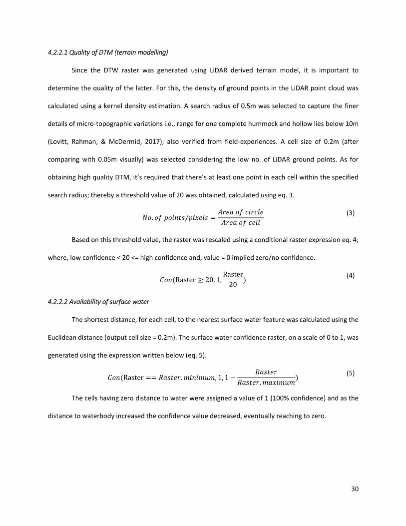
4.2.2.1 Quality of DTM (terrain modelling)
Since the DTW raster was generated using LiDAR derived terrain model, it is important to
determine the quality of the latter. For this, the density of ground points in the LiDAR point cloud was
calculated using a kernel density estimation. A search radius of 0.5m was selected to capture the finer
details of micro-topographic variations i.e., range for one complete hummock and hollow lies below 10m
(Lovitt, Rahman, & McDermid, 2017); also verified from field-experiences. A cell size of 0.2m (after
comparing with 0.05m visually) was selected considering the low no. of LiDAR ground points. As for
obtaining high quality DTM, it’s required that there’s at least one point in each cell within the specified
search radius; thereby a threshold value of 20 was obtained, calculated using eq. 3.
𝑁𝑜. 𝑜𝑓 𝑝𝑜𝑖𝑛𝑡𝑠/𝑝𝑖𝑥𝑒𝑙𝑠 =
𝐴𝑟𝑒𝑎 𝑜𝑓 𝑐𝑖𝑟𝑐𝑙𝑒
𝐴𝑟𝑒𝑎 𝑜𝑓 𝑐𝑒𝑙𝑙
(3)
Based on this threshold value, the raster was rescaled using a conditional raster expression eq. 4;
where, low confidence < 20 <= high confidence and, value = 0 implied zero/no confidence.
𝐶𝑜𝑛(Raster ≥ 20, 1,
Raster
20)
(4)
4.2.2.2 Availability of surface water
The shortest distance, for each cell, to the nearest surface water feature was calculated using the
Euclidean distance (output cell size = 0.2m). The surface water confidence raster, on a scale of 0 to 1, was
generated using the expression written below (eq. 5).
𝐶𝑜𝑛(Raster == 𝑅𝑎𝑠𝑡𝑒𝑟. 𝑚𝑖𝑛𝑖𝑚𝑢𝑚, 1, 1 −
𝑅𝑎𝑠𝑡𝑒𝑟
𝑅𝑎𝑠𝑡𝑒𝑟. 𝑚𝑎𝑥𝑖𝑚𝑢𝑚)
(5)
The cells having zero distance to water were assigned a value of 1 (100% confidence) and as the
distance to waterbody increased the confidence value decreased, eventually reaching to zero.
31
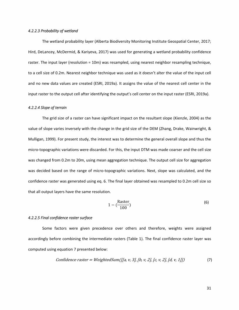
4.2.2.3 Probability of wetland
The wetland probability layer (Alberta Biodiversity Monitoring Institute Geospatial Center, 2017;
Hird, DeLancey, McDermid, & Kariyeva, 2017) was used for generating a wetland probability confidence
raster. The input layer (resolution = 10m) was resampled, using nearest neighbor resampling technique,
to a cell size of 0.2m. Nearest neighbor technique was used as it doesn’t alter the value of the input cell
and no new data values are created (ESRI, 2019a). It assigns the value of the nearest cell center in the
input raster to the output cell after identifying the output’s cell center on the input raster (ESRI, 2019a).
4.2.2.4 Slope of terrain
The grid size of a raster can have significant impact on the resultant slope (Kienzle, 2004) as the
value of slope varies inversely with the change in the grid size of the DEM (Zhang, Drake, Wainwright, &
Mulligan, 1999). For present study, the interest was to determine the general overall slope and thus the
micro-topographic variations were discarded. For this, the input DTM was made coarser and the cell size
was changed from 0.2m to 20m, using mean aggregation technique. The output cell size for aggregation
was decided based on the range of micro-topographic variations. Next, slope was calculated, and the
confidence raster was generated using eq. 6. The final layer obtained was resampled to 0.2m cell size so
that all output layers have the same resolution.
1 − (
Raster
100)
(6)
4.2.2.5 Final confidence raster surface
Some factors were given precedence over others and therefore, weights were assigned
accordingly before combining the intermediate rasters (Table 1). The final confidence raster layer was
computed using equation 7 presented below:
Confidence raster = WeightedSum([[a, v, 3], [b, v, 2], [c, v, 2], [d, v, 1]]) (7)
32
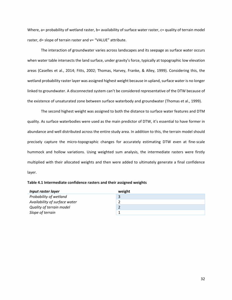
Where, a= probability of wetland raster, b= availability of surface water raster, c= quality of terrain model
raster, d= slope of terrain raster and v= “VALUE” attribute.
The interaction of groundwater varies across landscapes and its seepage as surface water occurs
when water table intersects the land surface, under gravity’s force, typically at topographic low elevation
areas (Caselles et al., 2014; Fitts, 2002; Thomas, Harvey, Franke, & Alley, 1999). Considering this, the
wetland probability raster layer was assigned highest weight because in upland, surface water is no longer
linked to groundwater. A disconnected system can’t be considered representative of the DTW because of
the existence of unsaturated zone between surface waterbody and groundwater (Thomas et al., 1999).
The second highest weight was assigned to both the distance to surface water features and DTM
quality. As surface waterbodies were used as the main predictor of DTW, it’s essential to have former in
abundance and well distributed across the entire study area. In addition to this, the terrain model should
precisely capture the micro-topographic changes for accurately estimating DTW even at fine-scale
hummock and hollow variations. Using weighted sum analysis, the intermediate rasters were firstly
multiplied with their allocated weights and then were added to ultimately generate a final confidence
layer.
Table 4.1 Intermediate confidence rasters and their assigned weights
Input raster layer weight
Probability of wetland 3
Availability of surface water 2
Quality of terrain model 2
Slope of terrain 1
33
Chapter 5: Results
5.1 GWL and DTW surfaces
Figure 5.1 represents the interpolated GWL surface with values ranging from 686.7m to 703.6m
(above mean sea level). As observed, the values decreased on moving from south-east towards north-
west; with highest GWL values clustered at the center of the study area. The lines visible in the map
depicts the variability in the data values which could be due to the availability of lesser water sample
points. The randomly selected additional set of water samples (or, testing data) consisting of 41 points
revealed an RMSE of approximately 19cm.

34
Figure 5.1 Continuous GWL surface obtained through interpolation of random water samples
The DTW surface (Figure 5.2) predicted using GWL surface ranged from 0 to 7.54 m. The entire
study area almost had water table at or near the surface (low DTW values) with few areas (such as, central
portion) having high values for DTW.

35
Figure 5.2 Final DTW surface obtained after rescaling
5.2 Confidence raster surface
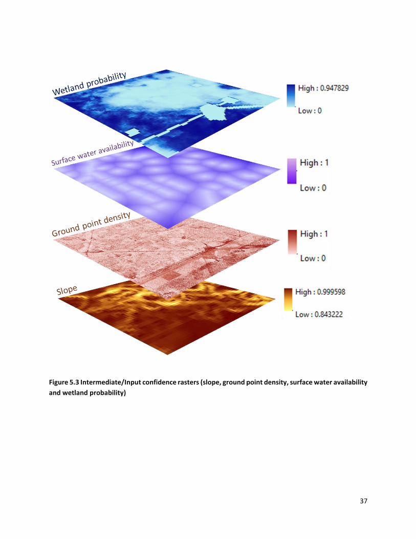
The four intermediate rasters (slope, quality of terrain, surface water availability and wetland
probability) and the final confidence raster surface are shown in Figures 5.3 and 5.4 respectively. The

36
individual interpretation of these resultant surfaces is done in the present section. The study area was
almost flat as observed from slope confidence raster results with high confident or, more flat areas
represented as dark brown. The slope values were variable at the middle portion of the study area (light
yellow to brown shades). A high confidence value for “ground point density/quality of terrain” confidence
raster imply that sufficient number of ground points are available for a terrain to be mapped accurately.
As per results, the terrain was mapped with high accuracies for seismic lines, roads and built-ups (dark
rust brown). Whereas moderate to low confidence in accuracy of terrain model was observed for
waterbodies and forested areas (lighter shades of brown). For surface water confidence raster, the water
cells having high confidence values have been represented by shades of light purple and as the distance
from the waterbody increased, the confidence value decreased represented as dark purple. More surface
water availability was observed in western portion of the study area. Whereas, upper north-eastern
corner had almost zero availability of water features. According to the wetland confidence raster, wetland
areas were less. The wetland probability values were represented as shades of blue, with dark blue areas
signifying high probability of an area being wetland and lighter shades depicting low wetland probability
i.e., area is less likely a wetland. As expected, the upland region (center portion) was classified as low
wetland probability. The final confidence raster value ranged from 1.72 to 7.7; with low confidence and
high confidence areas represented as shades of brown and purple respectively. We were less confident in
the DTW value predicted for uplands and significantly confident that the DTW value is accurate for
western part of the study region; which is basically wetland.
37
Figure 5.3 Intermediate/Input confidence rasters (slope, ground point density, surface water availability
and wetland probability)
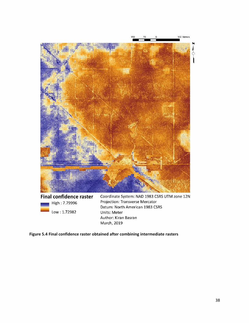
38
Figure 5.4 Final confidence raster obtained after combining intermediate rasters

39
Chapter 6: Discussion
Based on the confidence raster results, the method worked well in wetland and low confidence
was observed in upland. Due to the absence of field measurements no actual accuracy assessment of DTW
resultant layer was performed and the error estimation is based on confidence raster results. Although it
was assumed that all the input confidence rasters generated were correct; some issues were observed
and are discussed below. A lake in the wetland probability layer was observed to be classified as low
wetland probability class (Figure 6.1). Additionally, low lidar point densities for water features and
forested areas were observed (Figure 6.2). These contributed as sources of error in the final confidence
raster layer. This is to be noted however, the confidence layer results are based on logical analysis (built
on the assumptions that we had) and not a statistical approach. The present study results, however, were
in line with Rahman et al. (2017) who also observed errors in uplands and densely vegetated areas;
whereas, considerable better results were obtained for open areas (RMSE ~20 cm).
Figure 6.1 RGB-NIR orthophoto (left) with zoomed portion of lake (middle) and same area classified as
low wetland probability in the wetland probability layer (right)
Theoretically, the DTW value should be positive starting from 0; negative values for the resultant
DTW surface were obtained, however. This could be due errors in LiDAR derived terrain model as

40
explained below. The LiDAR data has lower point densities for water features because of data drop-out
issues (Höfle, Vetter, Pfeifer, Mandlburger, & Stötter, 2009; Toscano, Acharjee, & Mccormick, 2015) as
the surface reflectance properties affect the laser beam (Kashani, Olsen, Parrish, & Wilson, 2015). The
lower point densities lead to interpolation errors and ultimately generates artifacts in DEM (Worstell et
al., 2014). From the intermediate ‘quality of terrain’ confidence raster, we observed low confidence values
for some waterbodies signifying low LiDAR point densities (Figure 6.2).
Figure 6.2 Water feature on RGB-NIR orthophoto (left); same water feature on intermediate ‘quality of
terrain’ confidence raster
The laser data drop-out in water features could be due to 1) low spectral reflectance and 2)
specular/mirror-like reflection (Toscano et al., 2015). As LiDAR operates in near-infrared region, the
radiation is mostly absorbed by water feature thereby resulting into weak or no return i.e., low spectral
reflectance (Höfle et al., 2009; Toscano et al., 2015). Secondly, the radiation could either undergo specular
reflection, as in case of clear water (a smooth surface that acts as a highly reflective object) (Kashani et
al., 2015; Toscano et al., 2015); and thus being reflected away from the LiDAR receiver (Höfle et al., 2009).
The interaction of LiDAR with a waterbody depends upon the roughness of the water surface and it is
however possible to get some reflectance from water; when waves are present or if the water is turbid.
The multipath returns or, diffused reflection however, leads to time lag between incident and reflected
radiation; thus exceeding the detection threshold (Kashani et al., 2015). This might result in random
returns from the water surface (Parrot & Núñez, 2016) thus creating reflection underneath the surface of
41
waterbody that might not be representative of the actual surface properties (Kashani et al., 2015). This
shortcoming of LiDAR-DTM was considered and the negative DTW values were rescaled to zero.
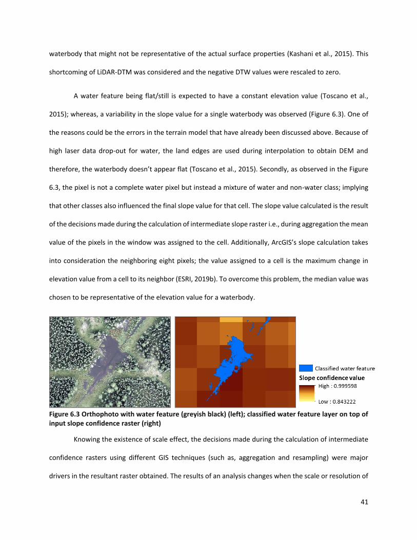
A water feature being flat/still is expected to have a constant elevation value (Toscano et al.,
2015); whereas, a variability in the slope value for a single waterbody was observed (Figure 6.3). One of
the reasons could be the errors in the terrain model that have already been discussed above. Because of
high laser data drop-out for water, the land edges are used during interpolation to obtain DEM and
therefore, the waterbody doesn’t appear flat (Toscano et al., 2015). Secondly, as observed in the Figure
6.3, the pixel is not a complete water pixel but instead a mixture of water and non-water class; implying
that other classes also influenced the final slope value for that cell. The slope value calculated is the result
of the decisions made during the calculation of intermediate slope raster i.e., during aggregation the mean
value of the pixels in the window was assigned to the cell. Additionally, ArcGIS’s slope calculation takes
into consideration the neighboring eight pixels; the value assigned to a cell is the maximum change in
elevation value from a cell to its neighbor (ESRI, 2019b). To overcome this problem, the median value was
chosen to be representative of the elevation value for a waterbody.
Figure 6.3 Orthophoto with water feature (greyish black) (left); classified water feature layer on top of input slope confidence raster (right)
Knowing the existence of scale effect, the decisions made during the calculation of intermediate
confidence rasters using different GIS techniques (such as, aggregation and resampling) were major
drivers in the resultant raster obtained. The results of an analysis changes when the scale or resolution of

42
the image is changed, and this irregularity in results is termed as scale effect- a sub problem of modifiable
areal unit problem (MAUP) (Fotheringham, & Rogerson, 2008). With change in scale, spatial
autocorrelation between variables also changes depending upon the aggregation level, higher
aggregation would result in higher spatial correlations (Fotheringham, & Rogerson, 2008). A new dataset
is created when the grid size is changed and thereby, multiple datasets are created this way leading to
different results (Fotheringham, & Rogerson, 2008). The complications associated with MAUP for
analyzing a spatial phenomenon, its implications on results were acknowledged and therefore due
consideration was given to this issue during the selection process. For instance, to obtain desirable results,
the LiDAR-DTM input in the present study was up-scaled prior slope calculation to discard variations in
microforms. Additional effort was made to determine the suitable scale for all output raster layers and,
be consistent throughout, as selection of appropriate scale may restrict MAUP effects (Dark & Bram,
2007). Therefore, it is suggested that the researchers should be aware of MAUP and examine it while
performing spatial analysis as different choices lead to different results.
6.1 Comparison between ‘present study DTW’ and wet areas mapping (WAM)
An attempt was made to compare our study with the already existing wet areas mapping (WAM)
technique. Our method estimated the GWT position to ultimately determine the DTW values. The WAM,
on the other hand, predicted the wet areas in relation to the “tendency of the soil to be saturated”
(Murphy, Ogilvie, Connor, & Arp, 2007, p. 849), with no reference to water table position. Thereby, this
study can be beneficial for researchers interested in conducting analysis that require the information
about the actual position of GWT. For instance, a hydrologist interested in tracking the DTW fluctuations
to determine the availability of groundwater, an eco-hydrologist studying the interactions between water
and environment or, a plant scientist interested in determining groundwater dependent ecosystems.
Other disciplines where the present research could be beneficial includes foresters, environmental
scientists, ecologists etc. The WAM-DTW provides additional information about stream channels and
43
networks, and thus can be useful for applications that particularly require visualizing wet areas; for
instance, mapping road-stream interactions, determining flow networks and channels etc. (White et al.,
2012).
The present method predicted the exact DTW value, at 0.2m resolution, for a given location and
the output is a continuous DTW raster. Additionally, an estimate of confidence values over varying
landcover classes was provided. Figure 6.4 presents the DTW values for the present study for high
confidence areas. The WAM however, is a static technique with a thematic representation of wet areas
(in the form of map), at 1m resolution, into different wetness classes with each class representing a range
of values (Figure 6.5). Their wet areas maps represent the areas that might be wet or, saturated for
significant duration of a year, specifically during wet seasons. DTW parameter being dynamic, changes
with changing weather conditions. Therefore, the present study can provide variable DTW information
and can be used for tracking DTW changes.
This study relies on certain assumptions that surface waterbodies are abundant and is tightly
connected to groundwater. Thereby, might not work in the absence of surface water features and is
suitable for making DTW prediction in low-lying areas primarily. Additionally, in the events of high
precipitation rates the surface water might not be reflective of actual groundwater levels. WAM on the
other hand is applicable under variable circumstances as their study is based on prediction using stream
channels, rivers, lakes etc. and topographic information.
The present study therefore, can be considered as an alternative to wet areas mapping technique;
that can be used as dynamic DTW monitoring tool.

44
Figure 6.4 Present study DTW values for high confidence areas

45
Figure 6.5 WAM layer for the present study area; with each class signifying the level of wetness
6.2 Future work
As the present method didn’t work well in certain areas (uplands), therefore, it can be suggested
to explore other techniques for mapping DTW particularly in low confidence areas and then combining it
with the present method. For instance, using the vegetation greenness as a proxy measure for predicting
DTW in forested areas. Also, If field data was available, a statistical accuracy assessment could be done by
extracting the DTW interpolated model values for the field samples and then comparing them against the
actual measurements ultimately calculating the error. Model validation could be beneficial in determining
how well the model performed in predicting the DTW values at unsampled locations.

46
Chapter 7: Conclusion
The present study attempted to test a workflow (Rahman et al., 2017), over a complex study area,
for mapping DTW using surface water as groundwater or, DTW predictor. Additionally, a confidence raster
surface was generated based on the following factors: slope of terrain, accuracy of terrain model,
availability of surface water and wetland probability. The method very well predicted DTW in wetland,
however, resulted in less confidence in uplands as evident from the final confidence raster results.
Compared to WAM, this technique is capable of providing dynamic DTW information and therefore could
aid in various disciplines such as, forestry, environment, botany, hydrology and eco-hydrology etc. The
present method however, has shortcomings as its applicable if surface water is present and tightly
connected to groundwater and therefore, can be considered as a supplement to WAM technique. Future
work can be conducted to map low confident areas using proxy measures such as soil moisture or,
vegetation information.
47
References
Agarwal, A. K., & Mishra, D. (1992). Evaluation of ground water potential in the environs of Jhansi city,
Uttar Pradesh using hydrogeomorphological assessment by satellite remote sensing technique.
Journal of the Indian Society of Remote Sensing, 20(2–3), 121–128.
https://doi.org/10.1007/BF02999208
Ahmadi, S. H., & Sedghamiz, A. (2007). Geostatistical analysis of spatial and temporal variations of
groundwater level. Environmental monitoring and assessment, 129(1-3), 277-294.
Alberta Biodiversity Monitoring Institute Geospatial Centre. (2017). “Boreal Wetland probability –
technical documentation.” Edmonton, Alberta, Canada. Retrieved from
https://www.abmi.ca/home/data-analytics/da-top/da-product-overview/GIS-Land-Surface/Boreal-
Wetland-Probability-Data.html
Alley, W. M., & Konikow, L. F. (2015). Bringing GRACE Down to Earth. Groundwater, 53(6), 826–829.
https://doi.org/10.1111/gwat.12379
Arslan, H. (2012). Spatial and temporal mapping of groundwater salinity using ordinary kriging and
indicator kriging : The case of Bafra Plain , Turkey. Agricultural Water Management, 113, 57–63.
https://doi.org/10.1016/j.agwat.2012.06.015
Bartels, S. F., Caners, R. T., Ogilvie, J., White, B., & Macdonald, S. E. (2018). Relating Bryophyte
Assemblages to a Remotely Sensed Depth-to-Water Index in Boreal Forests. Frontiers in Plant
Science, 9(June), 1–11. https://doi.org/10.3389/fpls.2018.00858
Becker, M. W. (2006). Potential for satellite remote sensing of ground water. Ground Water, 44(2), 306–
318. https://doi.org/10.1111/j.1745-6584.2005.00123.x
Béjar-Pizarro, M., Ezquerro, P., Herrera, G., Tomás, R., Guardiola-Albert, C., Ruiz Hernández, J. M., …
48
Martínez, R. (2017). Mapping groundwater level and aquifer storage variations from InSAR
measurements in the Madrid aquifer, Central Spain. Journal of Hydrology, 547, 678–689.
https://doi.org/10.1016/j.jhydrol.2017.02.011
Bjelanovic, I., Comeau, P. G., & White, B. (2018). High resolution site index prediction in boreal forests
using topographic and wet areas mapping attributes. Forests, 9(3).
https://doi.org/10.3390/f9030113
Bone, R. M. (2011): The Regional Geography of Canada. Fifth Edition. Oxford University Press.
Burrough, P. A., McDonnell, R., McDonnell, R. A., & Lloyd, C. D. (2015). Principles of geographical
information systems. Oxford university press.
Caselles, E., Pitarch, C., & Caselles, V. (2014). Estimation of the water table depth of the Calarasi district
Island (Romania) at the Danube River using ASTER/DEM data. European Journal of Remote Sensing,
47(1), 169–180. https://doi.org/10.5721/EuJRS20144711
Castellazzi, P., Longuevergne, L., Martel, R., Rivera, A., Brouard, C., & Chaussard, E. (2018). Quantitative
mapping of groundwater depletion at the water management scale using a combined GRACE/InSAR
approach. Remote Sensing of Environment, 205(November 2017), 408–418.
https://doi.org/10.1016/j.rse.2017.11.025
Castellazzi, P., Martel, R., Galloway, D. L., Longuevergne, L., & Rivera, A. (2016). Assessing Groundwater
Depletion and Dynamics Using GRACE and InSAR: Potential and Limitations. Groundwater, 54(6),
768–780. https://doi.org/10.1111/gwat.12453
Chen, F., Guo, H., Ma, P., Lin, H., Wang, C., Ishwaran, N., & Hang, P. (2017). Radar interferometry offers
new insights into threats to the Angkor site. Science Advances, 3(3), 1–9.
https://doi.org/10.1126/sciadv.1601284

49
Chen, J., Knight, R., Zebker, H. A., & Schreüder, W. A. (2016). Confined aquifer head measurements and
storage properties in the San Luis Valley, Colorado, from spaceborne InSAR observations. Water
Resources Research, 52(5), 3623-3636.
Chen, J., Zebker, H. A., & Knight, R. (2015). A persistent scatterer interpolation for retrieving accurate
ground deformation over InSAR-decorrelated agricultural fields. Geophysical Research Letters,
42(21), 9294–9301. https://doi.org/10.1002/2015GL065031
Chen, X., & Hu, Q. (2004). Groundwater influences on soil moisture and surface evaporation. Journal of
Hydrology, 297(1–4), 285–300. https://doi.org/10.1016/j.jhydrol.2004.04.019
Chowdhury, A., Jha, M. K., Chowdary, V. M., & Mal, B. C. (2008). Integrated remote sensing and GIS-based
approach for assessing groundwater potential in West Medinipur district, West Bengal, India.
International Journal of Remote Sensing, 30(1), 231–250.
https://doi.org/10.1080/01431160802270131
Condon, L. E., & Maxwell, R. M. (2015). Evaluating the relationship between topography and groundwater
using outputs from a continental‐scale integrated hydrology model. Water Resources
Research, 51(8), 6602-6621.
Cui, Y., & Shao, J. (2005). The role of ground water in arid/semiarid ecosystems, Northwest China. Ground
Water, 43(4), 471–477. https://doi.org/10.1111/j.1745-6584.2005.0063.x
Dark, S. J., & Bram, D. (2007). The modifiable areal unit problem (MAUP) in physical geography. Progress
in Physical Geography, 31(5), 471-479.
Deitchman, R. S., & Loheide, S. P. (2009). Ground-based thermal imaging of groundwater flow processes
at the seepage face. Geophysical Research Letters, 36(14), 1–6.
https://doi.org/10.1029/2009GL038103
50
Dettmann, U., & Bechtold, M. (2016). Deriving Effective Soil Water Retention Characteristicsfrom Shallow
Water Table Fluctuations in Peatlands. Vadose Zone Journal, 15(10), 0.
https://doi.org/10.2136/vzj2016.04.0029
Devi, P. S., Srinivasulu, S., & Raju, K. K. (2001). Hydrogeomorphological and groundwater prospects of the
Pageru river basin by using remote sensing data. Environmental Geology, 40(9), 1088-1094.
Downing, D. J., & Pettapiece, W. W. (2006). Natural Regions and Subregions of Alberta. Government of
Alberta.
Duan, L., Liu, T., Wang, X., & Luo, Y. (2015). Spatio-temporal patterns of water table and vegetation status
of a deserted area. Water (Switzerland), 7(10), 5788–5805. https://doi.org/10.3390/w7105788
ESRI. (2019a). In Cell size and resampling in analysis. Retrieved from desktop.arcgis.com website:
http://desktop.arcgis.com/en/arcmap/latest/extensions/spatial-analyst/performing-analysis/cell-
size-and-resampling-in-analysis.htm
ESRI. (2019b). In How Slope works. Retrieved from desktop.arcgis.com website:
http://desktop.arcgis.com/en/arcmap/10.3/tools/spatial-analyst-toolbox/how-slope-works.htm
Fitts, C. R. (2002). Groundwater science. Elsevier.
Fotheringham, A. S., & Rogerson, P. A. (Eds.). (2008). The SAGE handbook of spatial analysis. Sage.
Frappart, F., & Ramillien, G. (2018). Monitoring groundwater storage changes using the Gravity Recovery
and Climate Experiment (GRACE) satellite mission: A review. Remote Sensing, 10(6).
https://doi.org/10.3390/rs10060829
Gautam, A. M. (1990). Application of IRS-1A data for delineating buried channels in southern part of
Allahabad district of Uttar Pradesh. Journal of the Indian Society of Remote Sensing, 18(3), 52-55.
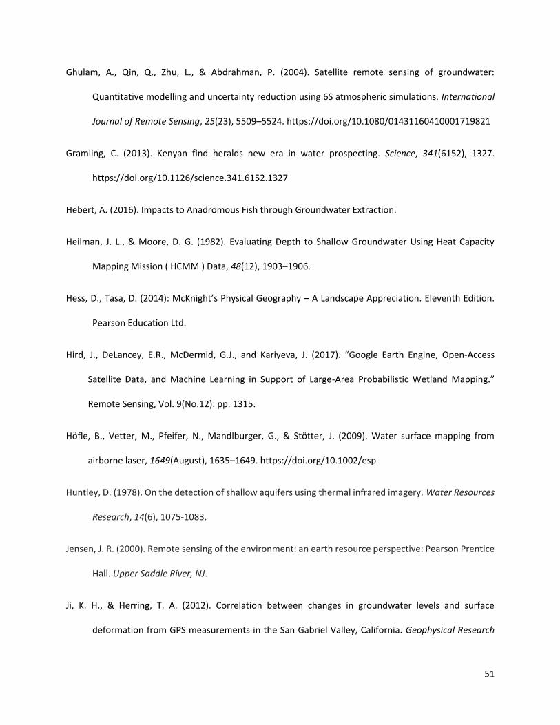
51
Ghulam, A., Qin, Q., Zhu, L., & Abdrahman, P. (2004). Satellite remote sensing of groundwater:
Quantitative modelling and uncertainty reduction using 6S atmospheric simulations. International
Journal of Remote Sensing, 25(23), 5509–5524. https://doi.org/10.1080/01431160410001719821
Gramling, C. (2013). Kenyan find heralds new era in water prospecting. Science, 341(6152), 1327.
https://doi.org/10.1126/science.341.6152.1327
Hebert, A. (2016). Impacts to Anadromous Fish through Groundwater Extraction.
Heilman, J. L., & Moore, D. G. (1982). Evaluating Depth to Shallow Groundwater Using Heat Capacity
Mapping Mission ( HCMM ) Data, 48(12), 1903–1906.
Hess, D., Tasa, D. (2014): McKnight’s Physical Geography – A Landscape Appreciation. Eleventh Edition.
Pearson Education Ltd.
Hird, J., DeLancey, E.R., McDermid, G.J., and Kariyeva, J. (2017). “Google Earth Engine, Open-Access
Satellite Data, and Machine Learning in Support of Large-Area Probabilistic Wetland Mapping.”
Remote Sensing, Vol. 9(No.12): pp. 1315.
Höfle, B., Vetter, M., Pfeifer, N., Mandlburger, G., & Stötter, J. (2009). Water surface mapping from
airborne laser, 1649(August), 1635–1649. https://doi.org/10.1002/esp
Huntley, D. (1978). On the detection of shallow aquifers using thermal infrared imagery. Water Resources
Research, 14(6), 1075-1083.
Jensen, J. R. (2000). Remote sensing of the environment: an earth resource perspective: Pearson Prentice
Hall. Upper Saddle River, NJ.
Ji, K. H., & Herring, T. A. (2012). Correlation between changes in groundwater levels and surface
deformation from GPS measurements in the San Gabriel Valley, California. Geophysical Research

52
Letters, 39(1), 1–5. https://doi.org/10.1029/2011GL050195
Ji, L., Zhang, L., & Wylie, B. (2009). Analysis of Dynamic Thresholds for the Normalized Difference Water
Index, 75(11), 1307–1317.
Johnson, D. G. (1992). USE OF GROUND-PENETRATING RADAR FOR WATER-TABLE MAPPING , BREWSTER
AND HARWICH , MASSACHUSETTS.
Kalacska, M., Arroyo-Mora, J. P., Soffer, R. J., Roulet, N. T., Moore, T. R., Humphreys, E., … Inamdar, D.
(2018). Estimating Peatland water table depth and net ecosystem exchange: A comparison between
satellite and airborne imagery. Remote Sensing, 10(5). https://doi.org/10.3390/rs10050687
Kashani, A. G., Olsen, M. J., Parrish, C. E., & Wilson, N. (2015). A Review of LIDAR Radiometric Processing:
From Ad Hoc Intensity Correction to Rigorous Radiometric Calibration, 28099–28128.
https://doi.org/10.3390/s151128099
Kerr, R. A. (2009). Northern India's Groundwater Is Going, Going, Going….
Kienzle, S. (2004). The Effect of DEM Raster Resolution on First Order , Second Order and Compound
Terrain Derivatives, 8(1), 83–111.
Koide, K., & Koike, K. (2012). Applying vegetation indices to detect high water table zones in humid warm-
temperate regions using satellite remote sensing. International Journal of Applied Earth
Observation and Geoinformation, 19(1), 88–103. https://doi.org/10.1016/j.jag.2012.03.017
Komarov, S. A., Mironov, V. L., Romanov, A. N., & Yevtyushkin, A. V. (1999). Remote Sensing of the water
table: Measurement and a data processing algorithm. Mapping Sciences and Remote
Sensing, 36(1), 1-10.
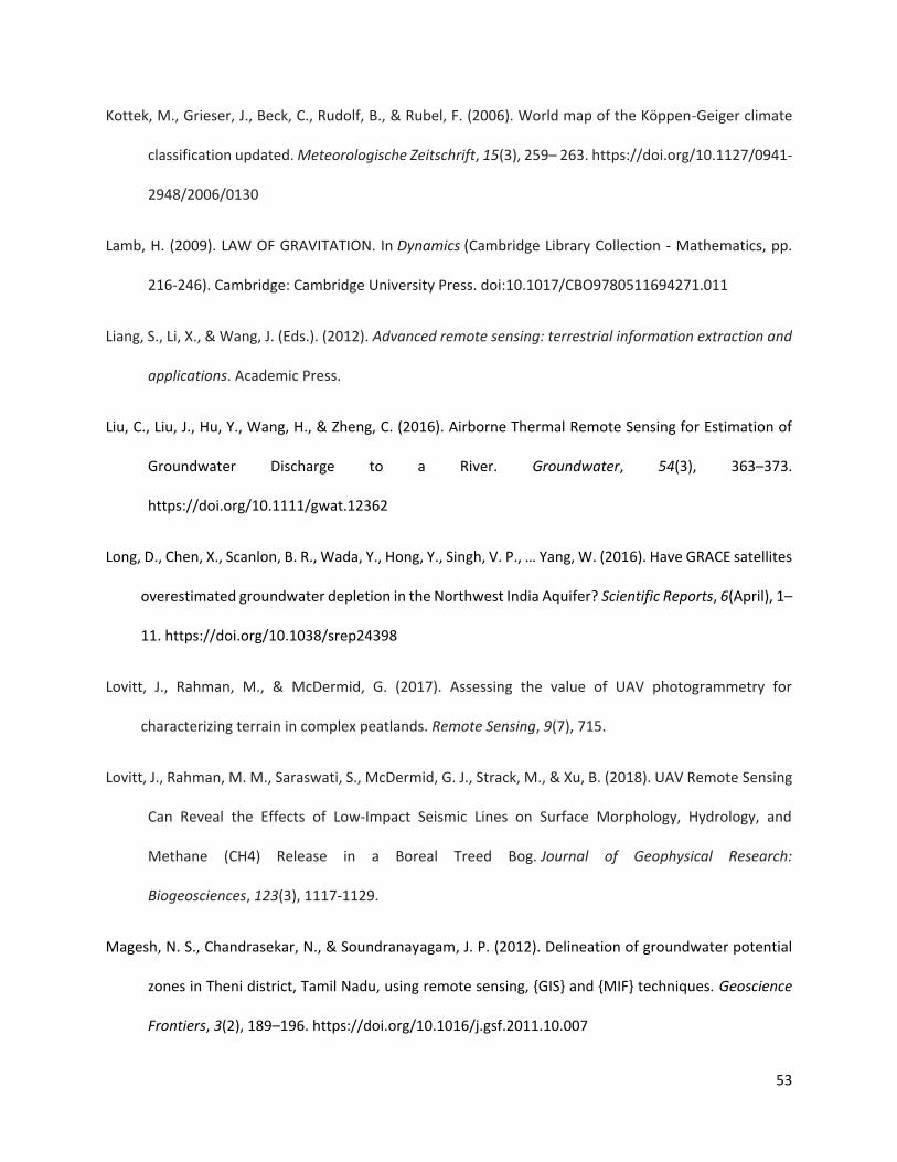
53
Kottek, M., Grieser, J., Beck, C., Rudolf, B., & Rubel, F. (2006). World map of the Köppen-Geiger climate
classification updated. Meteorologische Zeitschrift, 15(3), 259– 263. https://doi.org/10.1127/0941-
2948/2006/0130
Lamb, H. (2009). LAW OF GRAVITATION. In Dynamics (Cambridge Library Collection - Mathematics, pp.
216-246). Cambridge: Cambridge University Press. doi:10.1017/CBO9780511694271.011
Liang, S., Li, X., & Wang, J. (Eds.). (2012). Advanced remote sensing: terrestrial information extraction and
applications. Academic Press.
Liu, C., Liu, J., Hu, Y., Wang, H., & Zheng, C. (2016). Airborne Thermal Remote Sensing for Estimation of
Groundwater Discharge to a River. Groundwater, 54(3), 363–373.
https://doi.org/10.1111/gwat.12362
Long, D., Chen, X., Scanlon, B. R., Wada, Y., Hong, Y., Singh, V. P., … Yang, W. (2016). Have GRACE satellites
overestimated groundwater depletion in the Northwest India Aquifer? Scientific Reports, 6(April), 1–
11. https://doi.org/10.1038/srep24398
Lovitt, J., Rahman, M., & McDermid, G. (2017). Assessing the value of UAV photogrammetry for
characterizing terrain in complex peatlands. Remote Sensing, 9(7), 715.
Lovitt, J., Rahman, M. M., Saraswati, S., McDermid, G. J., Strack, M., & Xu, B. (2018). UAV Remote Sensing
Can Reveal the Effects of Low‐Impact Seismic Lines on Surface Morphology, Hydrology, and
Methane (CH4) Release in a Boreal Treed Bog. Journal of Geophysical Research:
Biogeosciences, 123(3), 1117-1129.
Magesh, N. S., Chandrasekar, N., & Soundranayagam, J. P. (2012). Delineation of groundwater potential
zones in Theni district, Tamil Nadu, using remote sensing, {GIS} and {MIF} techniques. Geoscience
Frontiers, 3(2), 189–196. https://doi.org/10.1016/j.gsf.2011.10.007
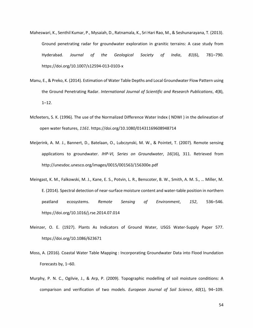
54
Maheswari, K., Senthil Kumar, P., Mysaiah, D., Ratnamala, K., Sri Hari Rao, M., & Seshunarayana, T. (2013).
Ground penetrating radar for groundwater exploration in granitic terrains: A case study from
Hyderabad. Journal of the Geological Society of India, 81(6), 781–790.
https://doi.org/10.1007/s12594-013-0103-x
Manu, E., & Preko, K. (2014). Estimation of Water Table Depths and Local Groundwater Flow Pattern using
the Ground Penetrating Radar. International Journal of Scientific and Research Publications, 4(8),
1–12.
Mcfeeters, S. K. (1996). The use of the Normalized Difference Water Index ( NDWI ) in the delineation of
open water features, 1161. https://doi.org/10.1080/01431169608948714
Meijerink, A. M. J., Bannert, D., Batelaan, O., Lubczynski, M. W., & Pointet, T. (2007). Remote sensing
applications to groundwater. IHP-VI, Series on Groundwater, 16(16), 311. Retrieved from
http://unesdoc.unesco.org/images/0015/001563/156300e.pdf
Meingast, K. M., Falkowski, M. J., Kane, E. S., Potvin, L. R., Benscoter, B. W., Smith, A. M. S., … Miller, M.
E. (2014). Spectral detection of near-surface moisture content and water-table position in northern
peatland ecosystems. Remote Sensing of Environment, 152, 536–546.
https://doi.org/10.1016/j.rse.2014.07.014
Meinzer, O. E. (1927). Plants As Indicators of Ground Water, USGS Water-Supply Paper 577.
https://doi.org/10.1086/623671
Moss, A. (2016). Coastal Water Table Mapping : Incorporating Groundwater Data into Flood Inundation
Forecasts by, 1–60.
Murphy, P. N. C., Ogilvie, J., & Arp, P. (2009). Topographic modelling of soil moisture conditions: A
comparison and verification of two models. European Journal of Soil Science, 60(1), 94–109.

55
https://doi.org/10.1111/j.1365-2389.2008.01094.x
Murphy, P. N. C., Ogilvie, J., Meng, F. R., White, B., Bhatti, J. S., & Arp, P. A. (2011). Modelling and mapping
topographic variations in forest soils at high resolution: A case study. Ecological Modelling, 222(14),
2314–2332. https://doi.org/10.1016/j.ecolmodel.2011.01.003
Murphy, P., Ogilvie, J., Connor, K., & Arp, P. (2007). Mapping Wetlands: A Comparison of Two Different
Approaches for New Brunswick, Canada. Wetlands, 27(4), 846–854. https://doi.org/10.1672/0277-
5212(2007)27[846:MWACOT]2.0.CO;2
Nas, B., & Berktay, A. (2010). Groundwater quality mapping in urban groundwater using GIS.
Environmental monitoring and assessment, 160(1-4), 215-227.
Ndou, N. N., Palamuleni, L. G., & Ramoelo, A. (2017). Modelling depth to groundwater level using SEBAL-
based dry season potential evapotranspiration in the upper Molopo River Catchment, South Africa.
Egyptian Journal of Remote Sensing and Space Science. https://doi.org/10.1016/j.ejrs.2017.08.003
Oltean, G. S., Comeau, P. G., & White, B. (2016). Soil Moisture on Boreal Forest Sites in Alberta, (April).
https://doi.org/10.5849/forsci.15-054
Pan, S. B., Wang, Z. J., Su, Q. X., Sun, T., & Zhang, Y. (2008). Groundwater Level Monitoring Model Using
Multi-Temporal Images in Arid Region of Northwest China. The International Archives of the
Photogrammetry, Remote Sensing and Spatial Information Sciences, 745–750. Retrieved from
http://www.isprs.org/proceedings/XXXVII/congress/8%7B_%7Dpdf/7%7B_%7DWG-VIII-7/04.pdf
Parrot, J., & Núñez, C. R. (2016). L i DAR DTM : artifacts , and correction for river altitudes Artefactos y
correcciones a los Modelos Digitales de Terreno provenientes del LiDAR. Investigaciones
Geográficas: Boletín Del Instituto de Geografía, 2016(90), 28–39.
https://doi.org/10.14350/rig.47372

56
Perkin, J. S., Gido, K. B., Falke, J. A., Fausch, K. D., Crockett, H., & Johnson, E. R. (2017). Groundwater
declines are linked to changes in Great Plains stream fish assemblages, 114(28), 7373–7378.
https://doi.org/10.1073/pnas.1618936114
Pfeffer, J., Seyler, F., Bonnet, M. P., Calmant, S., Frappart, F., Papa, F., ... & Silva, J. S. D. (2014). Low‐water
maps of the groundwater table in the central Amazon by satellite altimetry. Geophysical Research
Letters, 41(6), 1981-1987.
Rahman, M. M., McDermid, G. J., Strack, M., & Lovitt, J. (2017). A new method to map groundwater table
in peatlands using unmanned aerial vehicles. Remote Sensing, 9(10), 1–14.
https://doi.org/10.3390/rs9101057
Rokni, K., Ahmad, A., Selamat, A., & Hazini, S. (2014). Water Feature Extraction and Change Detection
Using Multitemporal Landsat Imagery, 4173–4189. https://doi.org/10.3390/rs6054173
Rai, B., Tiwari, A., & Dubey, V. S. (2005). Identification of groundwater prospective zones by using remote
sensing and geoelectrical methods in Jharia and Raniganj coalfields, Dhanbad district, Jharkhand
state. Journal of Earth System Science, 114(5), 515–522. https://doi.org/10.1007/BF02702027
Rashedi, E., Nezamabadi-pour, H., & Saryazdi, S. (2009). {GSA}: A {G}ravitational {S}earch {A}lgorithm.
Information Sciences, 179(13), 2232–2248. https://doi.org/10.1016/j.ins.2009.03.004
Rinderer, M., Van Meerveld, H. J., & Seibert, J. (2014). Topographic controls on shallow groundwater levels
in a steep, prealpine catchment: When are the TWI assumptions valid? Water Resources Research,
50(7), 6067–6080. https://doi.org/10.1002/2013WR015009
Ringrose, S., Vanderpost, C., & Matheson, W. (1998). Evaluation of vegetative criteria for near-surface
groundwater detection using multispectral mapping and GIS techniques in semi-arid Botswana.
Applied Geography, 18(4), 331–354. https://doi.org/10.1016/S0143-6228(98)00025-3

57
Saintenoy, A., & Hopmans, J. W. (2011). Ground Penetrating Radar: Water Table Detection Sensitivity to
Soil Water Retention Properties. IEEE Journal of Selected Topics in Applied Earth Observations and
Remote Sensing, 4(4), 748–753. https://doi.org/10.1109/JSTARS.2011.2171920
Sanderson, R. (2010). Introduction to remote sensing. New Mexico State University, 25-6.
Schwartz, F. W., & Zhang, H. (2003). Fundamentals of ground water. Wiley.
Seger, M. A., & Nashait, A. F. (2011). Detection of Water-Table by Using Ground Penetration Radar (GPR).
Eng. & Tech. Journal, 29(3), 554–566. https://doi.org/10.1002/anie.198505991
Sibanda, M., Dube, T., Seutloali, K., & Adelabu, S. (2015). Operational applications of remote sensing in
groundwater mapping across sub-Saharan Africa. Transactions of the Royal Society of South Africa,
70(2), 173–179. https://doi.org/10.1080/0035919X.2015.1017024
Stumpp, C., & Hose, G. C. (2013). The Impact of Water Table Drawdown and Drying on Subterranean
Aquatic Fauna in In-Vitro Experiments, 8(11). https://doi.org/10.1371/journal.pone.0078502
Sun, A. Y. (2013). Predicting groundwater level changes using GRACE data. Water Resources Research,
49(9), 5900–5912. https://doi.org/10.1002/wrcr.20421
Swenson, S., Famiglietti, J., Basara, J., & Wahr, J. (2008). Estimating profile soil moisture and groundwater
variations using GRACE and Oklahoma Mesonet soil moisture data. Water Resources Research,
44(1), 1–12. https://doi.org/10.1029/2007WR006057
Tempfli, K., Kerle, N., Huurneman, G. C., Janssen, L. L. F., Bakker, W. H., Feringa, W., … Woldai, T. (2009).
Text: Principles of Remote Sensing.
Thomas, C. W., Harvey, J. W., Franke, O. L., & Alley, W. A. (1999). Ground water and surface water, a single
resource. United States Geological Survey, Circular, 1139.

58
Toscano, G., Acharjee, P., McCormick, C., & Devarajan, V. (2015). Water Surface Elevation Calculation
Using LiDAR Data. In Proceedings, ASPRS Conference, Tampa, Florida.
Trenholm, N. M. (2000). The accuracy of water table elevation estimates determined from ground
penetrating radar data. Calgary.
White, B., Ogilvie, J., Campbell, D. M., Hiltz, D., Gauthier, B., Chisholm, H. K. H., ... & Arp, P. A. (2012). Using
the cartographic depth-to-water index to locate small streams and associated wet areas across
landscapes. Canadian Water Resources Journal/Revue canadienne des ressources hydriques, 37(4),
333-347.
Worstell, B. B., Poppenga, S., Evans, G. A., & Prince, S. (2014). Lidar point density analysis: implications for
identifying water bodies (No. 2014-5191). US Geological Survey.
Agarwal, A. K., & Mishra, D. (1992). Evaluation of ground water potential in the environs of Jhansi city,
Uttar Pradesh using hydrogeomorphological assessment by satellite remote sensing technique.
Journal of the Indian Society of Remote Sensing, 20(2–3), 121–128.
https://doi.org/10.1007/BF02999208
Alley, W. M., & Konikow, L. F. (2015). Bringing GRACE Down to Earth. Groundwater, 53(6), 826–829.
https://doi.org/10.1111/gwat.12379
Bartels, S. F., Caners, R. T., Ogilvie, J., White, B., & Macdonald, S. E. (2018). Relating Bryophyte
Assemblages to a Remotely Sensed Depth-to-Water Index in Boreal Forests. Frontiers in Plant
Science, 9(June), 1–11. https://doi.org/10.3389/fpls.2018.00858
Bechor, N. (2006). Extending interferometric synthetic aperture radar measurements from one to two
dimensions (Doctoral dissertation, Stanford University).
Becker, M. W. (2006). Potential for satellite remote sensing of ground water. Ground Water, 44(2), 306–

59
318. https://doi.org/10.1111/j.1745-6584.2005.00123.x
Béjar-Pizarro, M., Ezquerro, P., Herrera, G., Tomás, R., Guardiola-Albert, C., Ruiz Hernández, J. M., …
Martínez, R. (2017). Mapping groundwater level and aquifer storage variations from InSAR
measurements in the Madrid aquifer, Central Spain. Journal of Hydrology, 547, 678–689.
https://doi.org/10.1016/j.jhydrol.2017.02.011
Bjelanovic, I., Comeau, P. G., & White, B. (2018). High resolution site index prediction in boreal forests
using topographic and wet areas mapping attributes. Forests, 9(3).
https://doi.org/10.3390/f9030113
Caselles, E., Pitarch, C., & Caselles, V. (2014). Estimation of the water table depth of the Calarasi district
Island (Romania) at the Danube River using ASTER/DEM data. European Journal of Remote Sensing,
47(1), 169–180. https://doi.org/10.5721/EuJRS20144711
Castellazzi, P., Longuevergne, L., Martel, R., Rivera, A., Brouard, C., & Chaussard, E. (2018). Quantitative
mapping of groundwater depletion at the water management scale using a combined GRACE/InSAR
approach. Remote Sensing of Environment, 205(November 2017), 408–418.
https://doi.org/10.1016/j.rse.2017.11.025
Castellazzi, P., Martel, R., Galloway, D. L., Longuevergne, L., & Rivera, A. (2016). Assessing Groundwater
Depletion and Dynamics Using GRACE and InSAR: Potential and Limitations. Groundwater, 54(6),
768–780. https://doi.org/10.1111/gwat.12453
Chen, F., Guo, H., Ma, P., Lin, H., Wang, C., Ishwaran, N., & Hang, P. (2017). Radar interferometry offers
new insights into threats to the Angkor site. Science Advances, 3(3), 1–9.
https://doi.org/10.1126/sciadv.1601284

60
Chen, J., Knight, R., Zebker, H. A., & Schreüder, W. A. (2016). Confined aquifer head measurements and
storage properties in the San Luis Valley, Colorado, from spaceborne InSAR observations. Water
Resources Research, 52(5), 3623-3636.
Chen, J., Zebker, H. A., & Knight, R. (2015). A persistent scatterer interpolation for retrieving accurate
ground deformation over InSAR-decorrelated agricultural fields. Geophysical Research Letters,
42(21), 9294–9301. https://doi.org/10.1002/2015GL065031
Chen, X., & Hu, Q. (2004). Groundwater influences on soil moisture and surface evaporation. Journal of
Hydrology, 297(1–4), 285–300. https://doi.org/10.1016/j.jhydrol.2004.04.019
Chowdhury, A., Jha, M. K., Chowdary, V. M., & Mal, B. C. (2008). Integrated remote sensing and GIS-based
approach for assessing groundwater potential in West Medinipur district, West Bengal, India.
International Journal of Remote Sensing, 30(1), 231–250.
https://doi.org/10.1080/01431160802270131
Condon, L. E., & Maxwell, R. M. (2015). Evaluating the relationship between topography and groundwater
using outputs from a continental‐scale integrated hydrology model. Water Resources
Research, 51(8), 6602-6621.
Cui, Y., & Shao, J. (2005). The role of ground water in arid/semiarid ecosystems, Northwest China. Ground
Water, 43(4), 471–477. https://doi.org/10.1111/j.1745-6584.2005.0063.x
Deitchman, R. S., & Loheide, S. P. (2009). Ground-based thermal imaging of groundwater flow processes
at the seepage face. Geophysical Research Letters, 36(14), 1–6.
https://doi.org/10.1029/2009GL038103
Dettmann, U., & Bechtold, M. (2016). Deriving Effective Soil Water Retention Characteristicsfrom Shallow
Water Table Fluctuations in Peatlands. Vadose Zone Journal, 15(10), 0.

61
https://doi.org/10.2136/vzj2016.04.0029
Devi, P. S., Srinivasulu, S., & Raju, K. K. (2001). Hydrogeomorphological and groundwater prospects of the
Pageru river basin by using remote sensing data. Environmental Geology, 40(9), 1088-1094.
Duan, L., Liu, T., Wang, X., & Luo, Y. (2015). Spatio-temporal patterns of water table and vegetation status
of a deserted area. Water (Switzerland), 7(10), 5788–5805. https://doi.org/10.3390/w7105788
Fitts, C. R. (2002). Groundwater science. Elsevier.
Frappart, F., & Ramillien, G. (2018). Monitoring groundwater storage changes using the Gravity Recovery
and Climate Experiment (GRACE) satellite mission: A review. Remote Sensing, 10(6).
https://doi.org/10.3390/rs10060829
Gautam, A. M. (1990). Application of IRS-1A data for delineating buried channels in southern part of
Allahabad district of Uttar Pradesh. Journal of the Indian Society of Remote Sensing, 18(3), 52-55.
Ghulam, A., Qin, Q., Zhu, L., & Abdrahman, P. (2004). Satellite remote sensing of groundwater:
Quantitative modelling and uncertainty reduction using 6S atmospheric simulations. International
Journal of Remote Sensing, 25(23), 5509–5524. https://doi.org/10.1080/01431160410001719821
Gramling, C. (2013). Kenyan find heralds new era in water prospecting. Science, 341(6152), 1327.
https://doi.org/10.1126/science.341.6152.1327
Heilman, J. L., & Moore, D. G. (1982). Evaluating Depth to Shallow Groundwater Using Heat Capacity
Mapping Mission ( HCMM ) Data, 48(12), 1903–1906.
Huntley, D. (1978). On the detection of shallow aquifers using thermal infrared imagery. Water Resources
Research, 14(6), 1075-1083.

62
Jensen, J. R. (2000). Remote sensing of the environment: an earth resource perspective: Pearson Prentice
Hall. Upper Saddle River, NJ.
Ji, K. H., & Herring, T. A. (2012). Correlation between changes in groundwater levels and surface
deformation from GPS measurements in the San Gabriel Valley, California. Geophysical Research
Letters, 39(1), 1–5. https://doi.org/10.1029/2011GL050195
Johnson, D. G. (1992). USE OF GROUND-PENETRATING RADAR FOR WATER-TABLE MAPPING , BREWSTER
AND HARWICH , MASSACHUSETTS.
Kalacska, M., Arroyo-Mora, J. P., Soffer, R. J., Roulet, N. T., Moore, T. R., Humphreys, E., … Inamdar, D.
(2018). Estimating Peatland water table depth and net ecosystem exchange: A comparison between
satellite and airborne imagery. Remote Sensing, 10(5). https://doi.org/10.3390/rs10050687
Kerr, R. A. (2009). Northern India's Groundwater Is Going, Going, Going….
Kettridge, N., Turetsky, M. R., Sherwood, J. H., Thompson, D. K., Miller, C. A., Benscoter, B. W., ... &
Waddington, J. M. (2015). Moderate drop in water table increases peatland vulnerability to post-
fire regime shift. Scientific Reports, 5, 8063.
Koide, K., & Koike, K. (2012). Applying vegetation indices to detect high water table zones in humid warm-
temperate regions using satellite remote sensing. International Journal of Applied Earth
Observation and Geoinformation, 19(1), 88–103. https://doi.org/10.1016/j.jag.2012.03.017
Komarov, S. A., Mironov, V. L., Romanov, A. N., & Yevtyushkin, A. V. (1999). Remote Sensing of the water
table: Measurement and a data processing algorithm. Mapping Sciences and Remote
Sensing, 36(1), 1-10.
Lamb, H. (2009). LAW OF GRAVITATION. In Dynamics (Cambridge Library Collection - Mathematics, pp.
216-246). Cambridge: Cambridge University Press. doi:10.1017/CBO9780511694271.011
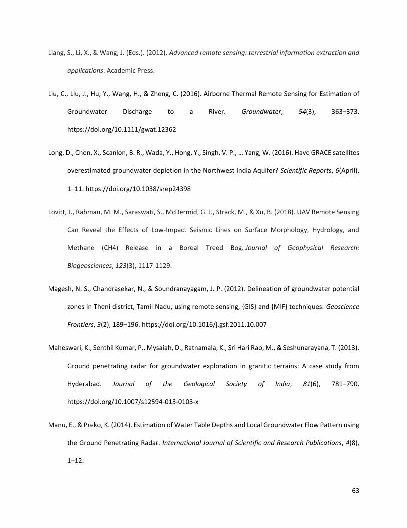
63
Liang, S., Li, X., & Wang, J. (Eds.). (2012). Advanced remote sensing: terrestrial information extraction and
applications. Academic Press.
Liu, C., Liu, J., Hu, Y., Wang, H., & Zheng, C. (2016). Airborne Thermal Remote Sensing for Estimation of
Groundwater Discharge to a River. Groundwater, 54(3), 363–373.
https://doi.org/10.1111/gwat.12362
Long, D., Chen, X., Scanlon, B. R., Wada, Y., Hong, Y., Singh, V. P., … Yang, W. (2016). Have GRACE satellites
overestimated groundwater depletion in the Northwest India Aquifer? Scientific Reports, 6(April),
1–11. https://doi.org/10.1038/srep24398
Lovitt, J., Rahman, M. M., Saraswati, S., McDermid, G. J., Strack, M., & Xu, B. (2018). UAV Remote Sensing
Can Reveal the Effects of Low‐Impact Seismic Lines on Surface Morphology, Hydrology, and
Methane (CH4) Release in a Boreal Treed Bog. Journal of Geophysical Research:
Biogeosciences, 123(3), 1117-1129.
Magesh, N. S., Chandrasekar, N., & Soundranayagam, J. P. (2012). Delineation of groundwater potential
zones in Theni district, Tamil Nadu, using remote sensing, {GIS} and {MIF} techniques. Geoscience
Frontiers, 3(2), 189–196. https://doi.org/10.1016/j.gsf.2011.10.007
Maheswari, K., Senthil Kumar, P., Mysaiah, D., Ratnamala, K., Sri Hari Rao, M., & Seshunarayana, T. (2013).
Ground penetrating radar for groundwater exploration in granitic terrains: A case study from
Hyderabad. Journal of the Geological Society of India, 81(6), 781–790.
https://doi.org/10.1007/s12594-013-0103-x
Manu, E., & Preko, K. (2014). Estimation of Water Table Depths and Local Groundwater Flow Pattern using
the Ground Penetrating Radar. International Journal of Scientific and Research Publications, 4(8),
1–12.

64
Meijerink, A. M. J., Bannert, D., Batelaan, O., Lubczynski, M. W., & Pointet, T. (2007). Remote sensing
applications to groundwater. IHP-VI, Series on Groundwater, 16(16), 311. Retrieved from
http://unesdoc.unesco.org/images/0015/001563/156300e.pdf
Meingast, K. M., Falkowski, M. J., Kane, E. S., Potvin, L. R., Benscoter, B. W., Smith, A. M. S., … Miller, M.
E. (2014). Spectral detection of near-surface moisture content and water-table position in northern
peatland ecosystems. Remote Sensing of Environment, 152, 536–546.
https://doi.org/10.1016/j.rse.2014.07.014
Meinzer, O. E. (1927). Plants As Indicators of Ground Water, USGS Water-Supply Paper 577.
https://doi.org/10.1086/623671
Miller, C. A., Benscoter, B. W., & Turetsky, M. R. (2015). The effect of long-term drying associated with
experimental drainage and road construction on vegetation composition and productivity in boreal
fens. Wetlands Ecology and Management, 23(5), 845–854. https://doi.org/10.1007/s11273-015-
9423-5
Murphy, P. N. C., Ogilvie, J., & Arp, P. (2009). Topographic modelling of soil moisture conditions: A
comparison and verification of two models. European Journal of Soil Science, 60(1), 94–109.
https://doi.org/10.1111/j.1365-2389.2008.01094.x
Murphy, P. N. C., Ogilvie, J., Meng, F. R., White, B., Bhatti, J. S., & Arp, P. A. (2011). Modelling and mapping
topographic variations in forest soils at high resolution: A case study. Ecological Modelling, 222(14),
2314–2332. https://doi.org/10.1016/j.ecolmodel.2011.01.003
Ndou, N. N., Palamuleni, L. G., & Ramoelo, A. (2017). Modelling depth to groundwater level using SEBAL-
based dry season potential evapotranspiration in the upper Molopo River Catchment, South Africa.
Egyptian Journal of Remote Sensing and Space Science. https://doi.org/10.1016/j.ejrs.2017.08.003

65
Oltean, G. S., Comeau, P. G., & White, B. (2016). Soil Moisture on Boreal Forest Sites in Alberta, (April).
https://doi.org/10.5849/forsci.15-054
Pan, S. B., Wang, Z. J., Su, Q. X., Sun, T., & Zhang, Y. (2008). Groundwater Level Monitoring Model Using
Multi-Temporal Images in Arid Region of Northwest China. The International Archives of the
Photogrammetry, Remote Sensing and Spatial Information Sciences, 745–750. Retrieved from
http://www.isprs.org/proceedings/XXXVII/congress/8%7B_%7Dpdf/7%7B_%7DWG-VIII-7/04.pdf
Pfeffer, J., Seyler, F., Bonnet, M. P., Calmant, S., Frappart, F., Papa, F., ... & Silva, J. S. D. (2014). Low‐water
maps of the groundwater table in the central Amazon by satellite altimetry. Geophysical Research
Letters, 41(6), 1981-1987.
Rahman, M. M., McDermid, G. J., Strack, M., & Lovitt, J. (2017). A new method to map groundwater table
in peatlands using unmanned aerial vehicles. Remote Sensing, 9(10), 1–14.
https://doi.org/10.3390/rs9101057
Rai, B., Tiwari, A., & Dubey, V. S. (2005). Identification of groundwater prospective zones by using remote
sensing and geoelectrical methods in Jharia and Raniganj coalfields, Dhanbad district, Jharkhand
state. Journal of Earth System Science, 114(5), 515–522. https://doi.org/10.1007/BF02702027
Rashedi, E., Nezamabadi-pour, H., & Saryazdi, S. (2009). {GSA}: A {G}ravitational {S}earch {A}lgorithm.
Information Sciences, 179(13), 2232–2248. https://doi.org/10.1016/j.ins.2009.03.004
Rinderer, M., Van Meerveld, H. J., & Seibert, J. (2014). Topographic controls on shallow groundwater levels
in a steep, prealpine catchment: When are the TWI assumptions valid? Water Resources Research,
50(7), 6067–6080. https://doi.org/10.1002/2013WR015009
Ringrose, S., Vanderpost, C., & Matheson, W. (1998). Evaluation of vegetative criteria for near-surface
groundwater detection using multispectral mapping and GIS techniques in semi-arid Botswana.
66
Applied Geography, 18(4), 331–354. https://doi.org/10.1016/S0143-6228(98)00025-3
Saintenoy, A., & Hopmans, J. W. (2011). Ground Penetrating Radar: Water Table Detection Sensitivity to
Soil Water Retention Properties. IEEE Journal of Selected Topics in Applied Earth Observations and
Remote Sensing, 4(4), 748–753. https://doi.org/10.1109/JSTARS.2011.2171920
Sanderson, R. (2010). Introduction to remote sensing. New Mexico State University, 25-6.
Schwartz, F. W., & Zhang, H. (2003). Fundamentals of ground water. Wiley.
Seger, M. A., & Nashait, A. F. (2011). Detection of Water-Table by Using Ground Penetration Radar (GPR).
Eng. & Tech. Journal, 29(3), 554–566. https://doi.org/10.1002/anie.198505991
Sibanda, M., Dube, T., Seutloali, K., & Adelabu, S. (2015). Operational applications of remote sensing in
groundwater mapping across sub-Saharan Africa. Transactions of the Royal Society of South Africa,
70(2), 173–179. https://doi.org/10.1080/0035919X.2015.1017024
Stromberg, J. C., Tiller, R., & Richter, B. (1996). Effects of groundwater decline on riparian vegetation of
semiarid regions: the San Pedro, Arizona. Ecological Applications, 6(1), 113-131.
Sun, A. Y. (2013). Predicting groundwater level changes using GRACE data. Water Resources Research,
49(9), 5900–5912. https://doi.org/10.1002/wrcr.20421
Swenson, S., Famiglietti, J., Basara, J., & Wahr, J. (2008). Estimating profile soil moisture and groundwater
variations using GRACE and Oklahoma Mesonet soil moisture data. Water Resources Research,
44(1), 1–12. https://doi.org/10.1029/2007WR006057
Tempfli, K., Kerle, N., Huurneman, G. C., Janssen, L. L. F., Bakker, W. H., Feringa, W., … Woldai, T. (2009).
Text: Principles of Remote Sensing.
Thenkabail, P. S. (Ed.). (2015). Remote sensing of water resources, disasters, and urban studies. CRC Press.

67
Thomas, C. W., Harvey, J. W., Franke, O. L., & Alley, W. A. (1999). Ground water and surface water, a single
resource. United States Geological Survey, Circular, 1139.
Trenholm, N. M. (2000). The accuracy of water table elevation estimates determined from ground
penetrating radar data. Calgary.
Xiang, L., Wang, H., Steffen, H., Wu, P., Jia, L., Jiang, L., & Shen, Q. (2016). Groundwater storage changes
in the Tibetan Plateau and adjacent areas revealed from GRACE satellite gravity data. Earth and
Planetary Science Letters. https://doi.org/10.1016/j.epsl.2016.06.002
Xiaomei, J., Li, W., Zhang, Y., Zhongqi, X. U. E., & Ying, Y. I. N. (2007). A study of the relationship between
vegetation growth and groundwater in the Yinchuan Plain. Earth Science Frontiers, 14(3), 197-203.
Xu, H. (2007). Extraction of Urban Built-up Land Features from Landsat Imagery Using a Thematic- oriented
Index Combination Technique, 73(12), 1381–1391.
Yao, L., Huo, Z., Feng, S., Mao, X., Kang, S., Chen, J., ... & Steenhuis, T. S. (2014). Evaluation of spatial
interpolation methods for groundwater level in an arid inland oasis, northwest China. Environmental
earth sciences, 71(4), 1911-1924.
Zhang, X., Drake, N. A., Wainwright, J., & Mulligan, M. (1999). COMPARISON OF SLOPE ESTIMATES FROM
LOW RESOLUTION DEMS : SCALING ISSUES AND A FRACTAL METHOD FOR THEIR SOLUTION, 779,
763–779.