mapp: the berkeley model and algorithm prototyping platform
TRANSCRIPT

J. Roychowdhury, University of California at Berkeley Slide 1
MAPP: The Berkeley Model and Algorithm Prototyping
Platform
Jaijeet Roychowdhury Tianshi Wang
EECS DepartmentUniversity of California at Berkeley

J. Roychowdhury, University of California at Berkeley Slide 2
Motivation for MAPP
Developing good compact models: many pitfalls» examples: discontinuities/smoothness, well-
posedness (has transient solution?)– problems usually discovered at deployment (ie, during
simulation)
» problems often hard to debug and resolve– compact model developer blames simulator
– simulator people blame the model
One goal of MAPP: to ease this problem» In MATLAB
– empowers non-programmers to debug models
– case studies + knowledge base → find solution to common problems (and try in MAPP) quickly

J. Roychowdhury, University of California at Berkeley Slide 3
MAPP for Device Model Development
CompactModel
Equations
Write in MATLAB(ModSpec format)
Run SmallCircuits in
MAPP
Testimmediately(standalone)
Problems?Yes
basic debugcode/facilitiesfor inspectionand debugging
➔ model doesn't evaluate➔ overflow/domain errors
➔ DC conv. failure➔ transient timestep too small➔ unphysical results➔ voltage/current blows up
➔ smoothing➔ define custom functions/derivatives➔ custom init/limiting➔ gmin
➔ format itself eliminates somecommon modelling mistakes
DC/AC/TRANin MATLAB
No

J. Roychowdhury, University of California at Berkeley Slide 4
Glimpse: ModSpec Device Definition
CompactModel
Equations
Write in MATLAB(ModSpec format)
Run SmallCircuits in
MAPP
Testimmediately(standalone)
basic debug
➔ format itself eliminates somecommon modelling mistakes

J. Roychowdhury, University of California at Berkeley Slide 5
CompactModel
Equations
Write in MATLAB(ModSpec format)
Run SmallCircuits in MDE
(Model DevelopmentEnvironment)
Testimmediately(standalone)
basic debug
➔ format itself eliminates somecommon modelling mistakes
Glimpse: Circuit Netlist in MAPP

J. Roychowdhury, University of California at Berkeley Slide 6
MAPP Model Development Flow (2)
ModSpec Model(in MATLAB)hand-coded
NEEDS-compatibleVerilog-A model
translate manually
to NEEDS-compatible Verilog-A
Step 2
ModSpec Model(in MATLAB)
auto-generatedfrom Verilog-A
automatic translatordouble-check
in MAPP
compare code, check consistency
Step 1: model developed in ModSpec/MAPP
end of Step 2: high level of confidence Verilog-A model is correct/debugged
J. Roychowdhury, University of California at Berkeley Slide 7
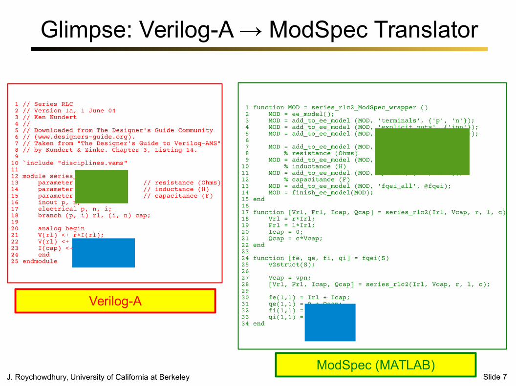
Glimpse: Verilog-A → ModSpec Translator
1 // Series RLC 2 // Version 1a, 1 June 04 3 // Ken Kundert 4 // 5 // Downloaded from The Designer's Guide Community 6 // (www.designers-guide.org). 7 // Taken from "The Designer's Guide to Verilog-AMS" 8 // by Kundert & Zinke. Chapter 3, Listing 14. 9 10 `include "disciplines.vams" 11 12 module series_rlc2 (p, n); 13 parameter real r=1000; // resistance (Ohms) 14 parameter real l=1e-9; // inductance (H) 15 parameter real c=1e-6; // capacitance (F) 16 inout p, n; 17 electrical p, n, i; 18 branch (p, i) rl, (i, n) cap; 19 20 analog begin 21 V(rl) <+ r*I(rl); 22 V(rl) <+ ddt(l*I(rl)); 23 I(cap) <+ ddt(c*V(cap)); 24 end 25 endmodule
1 function MOD = series_rlc2_ModSpec_wrapper () 2 MOD = ee_model(); 3 MOD = add_to_ee_model (MOD, 'terminals', {'p', 'n'}); 4 MOD = add_to_ee_model (MOD, 'explicit_outs', {'ipn'}); 5 MOD = add_to_ee_model (MOD, 'internal_unks', {'Irl'}); 6 7 MOD = add_to_ee_model (MOD, 'parms', {'r', 1000}); 8 % resistance (Ohms) 9 MOD = add_to_ee_model (MOD, 'parms', {'l', 1e-9}); 10 % inductance (H) 11 MOD = add_to_ee_model (MOD, 'parms', {'c', 1e-6}); 12 % capacitance (F) 13 MOD = add_to_ee_model (MOD, 'fqei_all', @fqei); 14 MOD = finish_ee_model(MOD); 15 end 16 17 function [Vrl, Frl, Icap, Qcap] = series_rlc2(Irl, Vcap, r, l, c) 18 Vrl = r*Irl; 19 Frl = l*Irl; 20 Icap = 0; 21 Qcap = c*Vcap; 22 end 23 24 function [fe, qe, fi, qi] = fqei(S) 25 v2struct(S); 26 27 Vcap = vpn; 28 [Vrl, Frl, Icap, Qcap] = series_rlc2(Irl, Vcap, r, l, c); 29 30 fe(1,1) = Irl + Icap; 31 qe(1,1) = 0 + Qcap; 32 fi(1,1) = vpn - Vrl; 33 qi(1,1) = 0 - Frl; 34 end
Verilog-A
ModSpec (MATLAB)

J. Roychowdhury, University of California at Berkeley Slide 8
MAPP Model Development Flow (3)
Step 3
NEEDS-compatibleVerilog-A model
(from Step 2)
use modelin Commercial
Simulators
ModSpecModel
(C++ API)
automatictranslator
model supportedin Open-source
Simulators(Xyce)
proof of modelgoodness
confirmmodel with
DC/AC/TRANin C++ MAPP
“simulation-ready” model deployed

J. Roychowdhury, University of California at Berkeley Slide 9
Glimpse: ModSpec Model in Xyce
1 *** Test-bench for generting dc response of an inverter 2 3 *** Creat sub-circuit for the inverter 4 .subckt inverter Vin Vout Vvdd Vgnd 5 6 yModSpec_Device X1 Vvdd Vin Vout Vvdd MVSmod type=-1 W=1.0e-4 7 Lgdr=32e-7 dLg=8e-7 Cg=2.57e-6 beta=1.8 alpha=3.5 Tjun=300 8 Cif = 1.38e-12 Cof=1.47e-12 phib=1.2 gamma=0.1 mc=0.2 9 CTM_select=1 Rs0=100 Rd0 = 100 n0=1.68 nd=0.1 vxo=7542204 10 mu=165 Vt0=0.5535 delta=0.15 11 12 yModSpec_Device X0 Vout Vin Vgnd Vgnd MVSmod type=1 W=1e-4 13 Lgdr=32e-7 dLg=9e-7 Cg=2.57e-6 beta=1.8 alpha=3.5 Tjun=300 14 Cif=1.38e-12 Cof=1.47e-12 phib=1.2 gamma=0.1 mc=0.2 15 CTM_select=1 Rs0=100 Rd0=100 n0=1.68 nd=0.1 vxo=1.2e7 16 mu=200 Vt0=0.4 delta=0.15 17 18 .model MVSmod MODSPEC_DEVICE SONAME=MVS_ModSpec_Element.so 19 20 .ends 21 22 *** circuit layout 23 Vsup sup 0 1 24 Vin in 0 0 25 Vsource source 0 0 26 X2 in out sup 0 inverter 27 28 *** simulation 29 .dc Vin 0 1 0.01 30 31 .print dc V(in) V(out) 32 *** END 33 .end
model's name model parameter:name of .so library
.model line
Xyce netlist for inverter(using MVS ModSpec/C++ model)
ModSpec Model(C++ API)
model supported in Xyce
.so libraries(dynamically loadable)
compile standalone
Xyce-ModSpecInterface
DC sweep using Xyce

J. Roychowdhury, University of California at Berkeley Slide 10
opto-electronicdevices
ModSpec: Multi-Physics Support
ModSpec Core(Equations)
Electrical
Electrical
Network Interface Layer
node voltages, branch currents,
KCL, KVL
OpticalOptical
Network Interface Layer
electric fields, polarizations,
modes, wavelengths,
wave continuity, ...
MechanicalMechanicalNILNIL
SpintronicSpintronicNILNIL
BiochemicalBiochemicalNILNIL
ThermalThermalNILNIL

J. Roychowdhury, University of California at Berkeley Slide 11
Optical System Modelling/Simulation Example

J. Roychowdhury, University of California at Berkeley Slide 12
MAPP: First Public Release
Open Source download: http://mapp.eecs.berkeley.edu» mailing list (MAPP announcements/discussion)» bug reporting and tracking site» git repository access (you can contribute)
License» primary: GPL-v3
» alternative licensing available– eg, SRC contract terms apply for SRC company use
» contributors can specify their own alternative licensing terms for their contributions

J. Roychowdhury, University of California at Berkeley Slide 13
MAPP: Features
Entirely in MATLAB Help system (start with help MAPP)
» quick start walk-through
Automatic differentiation (vecvalder)» help MAPPautodiff
Executable device specification (ModSpec)» examples, tutorial: part of help
DC, AC, transient analyses» also noise, homotopy, HB, shooting, PPV, MOR, etc. (not
released yet)
Automated testing system exercising suite of tests

J. Roychowdhury, University of California at Berkeley Slide 14
MAPP: Intended Uses
Developing simulation-ready device models» including multi-physics devices, network connectivity
Quickly prototyping new simulation algorithms» hours/days to implement a new analysis
– assess strengths/limitations before investing resources to implement in “real simulators”
» MAPP's structuring is different from SPICE's– devices “don't know about” algorithms; and vice-versa– central concept: DAEs (connect analyses and devices)
Learning or teaching modelling/simulation» MATLAB → broadly accessible» help system, tutorials, supporting resources

J. Roychowdhury, University of California at Berkeley Slide 15
mapp.eecs.berkeley.edu