MapDisto version 1.7

Tutorial[Draft version v. 1.0]

Mathias Lorieux

contact: mapdisto@gmail.com

September 2008

2

Table of contents.............................................................................................................................Acknowledgements 4

........................................................................................................................................Introduction 5....................................................................................................................................................What is MapDisto? 5

..............................................................................................................................................................Main features 5........................................................................................................Is MapDisto compatible with my computer? 6

.............................................................................................................................................................Why in Excel? 6.............................................................................................................................................How to cite MapDisto? 6

..........................................................................................................................................Installation 7......................................................................................................................The MapDisto interface 7

...........................................................................................................................................................About window 7...................................................................................................................................................Main menu window 7

..............................................................................................................................................................Data window 8........................................................................................................................................Color Genotypes window 9

..................................................................................................................................................Simulations window 9............................................................................................................................................Compare maps window 9

.................................................................................................................................................Extract map window 9..........................................................................................................................................Framework map window 9

...........................................................................................................................................................Result windows 9.....................................................................................................................................................................Toolbars 10

.............................................................................................................Data format and preparation 11..............................................................................................................................................................Data format 11

.................................................................................................................Importing a Mapmaker/EXP data file 11....................................................................................................................Creating a data file within MapDisto 11

......................................................................................................................................Managing several data sets 13......................................................................................................................Building a genetic map 13

...................................................................................................................................................Step 1: Preparation 13........................................................................................................................Step 2: Finding the linkage groups 14......................................................................................................................Step 3: Ordering the linkage groups 14

.......................................................................................................................................Step 4: Refining the order 15..........................................................................................................Advanced mapping operations 15

...........................................................................................................................Verifying Mendelian segregation 15................................................................................................................................................Visualize map details 15

.....................................................................................................................................Checking for order solidity 15...................................................................................................................................Identifying problematic loci 16

.................................................................................................................................Identifying genotyping errors 16......................................................................................................................Dealing with segregation distortion 16

.................................................................Comparing a computed genetic map to a reference map 16..................................................Assessing the effect of erroneous data fraction using simulations 17

................................................................................................................Looking for QTL locations 17.................................................Exporting a map created in MapDisto for QTL analysis programs 18

.................................................................................................Exporting data for Mapmaker/EXP 18...................................................................................Importing a map created in another program 18

..........................................................................................................................Command reference 19................................................................................................................Commands in the main menu window 19

............................................................................................................................Commands in the Data window 21..............................................................................................................Commands in the My sequences section 21

.................................................................................................................................Commands in import map… 21

MapDisto tutorial

3

..............................................................................................................................MapDisto options 22................................................................................................................................Troubleshooting 22

..........................................................................................................................................Macros are not active… 22.................................................................The program generates errors when I modify some parameters… 23

...................................................................................................Annex 1: Methods for ordering loci 24..........................................................................................................................................References 26

MapDisto tutorial

4

AcknowledgementsI’d like to thank Stéphane Dussert, Jean-François Rami and Bernard Rey for their kind and valuable help in Visual Basic commands.

Several people gave me important feedback and ideas to improve MapDisto. I'd like to give special thanks to Denis Lespinasse, Issa Coulibaly, Amidou N'Diaye and Kamel Langar, for their time and patience.

Finally, I can't forget Diego González de León, who initiated me to the field of genetic mapping theory. Hi, Diego!

MapDisto tutorial

5

Introduction

What is MapDisto?

Very efficient and powerful software such as Mapmaker/EXP, MapManager, GMendel or Carthagene have been developed –!and made freely available!– to construct genetic maps from linkage data of experimental segregating populations.

However, using these programs is not always intuitive and to learn how to deal with their commands can be time-consuming.

Moreover, no or limited options are proposed in these programs to deal with genetic markers that show deviations from expected Mendelian frequencies in their segregation ratios.

Thus, MapDisto is another free genetic mapping program that offers several powerful tools to compute and draw genetic maps easily and quickly through an intuitive graphical interface, and that facilitate the analysis of marker data showing segregation distortion due to differential viability of gametes or zygotes.

Main features

The present version (1.7) of MapDisto handles for several types of segregating populations, including backcross (BC1), doubled haploid (DH), recombinant inbred by single-seed descent (SSD), intermated recombinant inbred lines (IRIL), and F2 (intercross).

The program allows to:

-!Find linkage groups, with specified minimum LOD score and maximum recombination frequency,

-!Automatically order loci on linkage groups using one of the three available algorithms,

- Compute tables of recombination fractions (various estimates), map distances in centimorgans, linkage and independence khi2s, two-point LOD scores, correlations, for all couples of loci in a sequence,

- Compute segregation khi2s that measure the deviation from expected Mendelian segregation and their associated probabilities for all loci of a particular sequence,

-!Compute several map parameters for a specified sequence,

-!Look for genotyping errors and correct them,

-!Draw genetic maps computed either by MapDisto or imported from another program,

-!Find QTLs using one-way ANOVA and display a graphical output,

-!Export data and run (.in) files for MapMaker/EXP,

-!Export computed maps and data for advanced QTL analysis programs such as QTL Cartographer, WinQTLCart, QGene, or MapQTL,

-!Run automated commands that make the computation of an entire genetic map very fast and easy,

-!Compare maps,

-!And many other things that you will discover while reading this document.

The graphical interface permits us to easily manage various data sets and to navigate quickly between the different output windows.

A build-in quick help is included, which describes the main features of the program and the main steps to follow for data analysis. However, for a more detailed help, please refer to this manual.

MapDisto tutorial

6

Is MapDisto compatible with my computer?

I hope so! If not, you’ll probably find around a MS Windows machine with Excel. MapDisto has been developed in Microsoft Visual Basic for Applications (VBA) and needs any version of Microsoft Excel higher to 97 to run properly. It works well on Windows and Mac OS platforms (Mac OS X included). However, some users may experience minor incompatibility problems, especially with localized versions of Excel (see the “Troubleshooting” section).

Note: Maybe a future version will run in OpenOffice.org or NeoOffice, but it is not planned at this time. So far, the full compatibility with VBA code is still a way from being reached.

Note 2: A special version for Excel 2007 is available, although still in beta verion. The advantage of running MapDisto in Excel 2007 is mainly that it allows you to handle for bigger data sets (one million rows and 16,000+ columns actually – well, let’s see who can generate a such big data file!). However, I have found that MapDisto is quite slower in the newer version of Excel. Also, the MapDisto Toolbars are now located in the “Adds-Ins” sections of the Ribbon, which I don’t find very user-friendly. I would have preferred by far to have a new Excel that handles for 16,000 columns but that looks like Excel 2003 or 2004 and that would be at least as fast as its ancestors…

Why in Excel?

Well… Because when I started to program my own mapping routines, I found it very convenient to be able to go back and forth from the data to the analysis using Excel macros.

Since I started to distribute this program, many people encouraged me to pursue the development of MapDisto, and one of the features they liked in this program is precisely this ability to alter the data and analyze them on-the-fly.

Many researchers manage their data in spreadsheets programs, often in Excel. Thus, there is no need to prepare complex data files, since all you need is to copy and paste the data matrix from the worksheet that contains your data to the “Data” window of MapDisto, et voilà.

Also, the installation of the program could not be easier: just copy it to any folder.

However, with the announcement from Microsoft that they will discontinue the support of Visual Basic in Office 2008, the last edition for the Mac OS X operating system, my hope is that OpenOffice.org /NeoOffice will really bring a full support to the VBA code in the near future. Otherwise, the Mac users will have to stick with Office 2004, which is quite slow on the new Intel-based machines as it runs in emulation mode of the PowerPC processor. Or, they will have to use a virtual machine to run the Windows edition. Having VBA supported in OpenOffice.org would also probably mean that MapDisto could run in Linux, which would be really great.

How to cite MapDisto?

I’m currently preparing a paper about MapDisto, that I’ll try to publish in a peer-reviewed journal. Until this happens (...), you can use one of the following references:

Lorieux M. (2006) MapDisto, A Tool for Easy Mapping of Genetic Markers. Poster (P886) presented at the Plant and Animal Genome XIV conference, Jan 14-18 2006, San Diego, CA. URL: http://mapdisto.free.fr/.

Lorieux M. (2007) MapDisto, A Free User-Friendly Program For Computing Genetic Maps. Computer demonstration (P958) given at the Plant and Animal Genome XV conference, Jan 13-17 2007, San Diego, CA. URL: http://mapdisto.free.fr/.

MapDisto tutorial

7

InstallationFirst, download the program at http://mapdisto.free.fr/. Go to the section Download, and follow the instructions. Registering to the users list is optional, but this will give you the advantage of receiving information about future updates of the program.

When you are done with the downloading, I suggest creating a separate folder per mapping project on your hard disk. This folder will contain all the files related to your mapping project. Thereafter in this document, we will refer to this folder as MapFolder. Uncompress the downloaded file mapdisto.zip or

mapdistobeta.zip and place the resulting uncompressed files in MapFolder you just created.

The compressed file format is the Zip one, that you can uncompress on Mac OS X with a double-click, and on Windows XP with a right-click followed by the command Extract all…. On Microsoft Windows 2000, use the program WinZip.

The MapDisto interface

About window

This is the splash screen that is displayed when you open MapDisto (Figure 1). Click on Start to be

taken to the Main menu window.

Figure 1. The About window

Main menu window

This window is the heart of MapDisto: it will contain all the loci sequences that represent the linkage groups of the genetic map, and all the buttons that let you run the majority of the commands of the program. It also displays the main parameters of the segregating population, the genotype codes and the main options and parameters that are currently selected (Figure 2).

Generally, this window is accessed using the Commands button.

MapDisto tutorial

8

Figure 2. The Main menu window

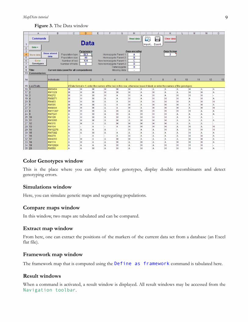
Data window

This window contains the genotyping data of the segregating population data that will be used for all subsequent computations (Figure 3). If the data are made of more that 254 loci or individuals, the

remaining of the data are put in the Data+ window. The Store data command allows saving the current data in another sheet that can be accessed with the Show stored data command.

MapDisto tutorial

9

Figure 3. The Data window

Color Genotypes window

This is the place where you can display color genotypes, display double recombinants and detect genotyping errors.

Simulations window

Here, you can simulate genetic maps and segregating populations.

Compare maps window

In this window, two maps are tabulated and can be compared.

Extract map window

From here, one can extract the positions of the markers of the current data set from a database (an Excel flat file).

Framework map window

The framework map that is computed using the Define as framework command is tabulated here.

Result windows

When a command is activated, a result window is displayed. All result windows may be accessed from the Navigation toolbar.

MapDisto tutorial

10

Toolbars

MapDisto has four toolbars that you may show or hide using the corresponding commands in the Main

Menu window.

The Navigation toolbar is used to display the different windows of the program.

The Commands toolbar allows running the most important commands of the program, even if another window than the “Main menu” window is displayed.

The Mini toolbar allows accessing the About window, the Main menu, the Navigation and Commands toolbars, the Options and Help window.

The Zoom toolbar is shown when a graphic (genetic map) is displayed.

Figure 4. The Navigation and Commands toolbars

Figure 5. The Mini toolbar

Figure 6. The Zoom toolbar

MapDisto tutorial

11

Data format and preparation

Data format

The data format of the Data window is, in essence, very similar to that of the Mapmaker/EXP data: it’s a matrix of n individuals x by m loci. The main difference with the Mapmaker/EXP format resides in the fact that you are not forced to have the loci distributed as rows in the data file: you may also prepare your data with the loci arranged as columns. In this case, just enter the value 1 in the Data format field.

Excel limitation: if you are running MapDisto within a version of Excel prior to 2007, the file size is limited to 508 for n or m, depending on the way the data are arranged. If the loci are distributed in rows, the limits are 508 individuals and 65,521 loci. If the loci are arranged in columns, then the limits are 508

loci and 65,521 individuals. Moreover, as the Excel sheets are limited to 256 columns, adding a Data+ window was the only way to handle with up to 512 columns, including the headers.

Importing a Mapmaker/EXP data file

The first option for preparing the genotyping data is to simply import a file formatted for the Mapmaker/EXP program. This format looks like in Figure 7.

Figure 7. Example of a genotyping data file for an F2 population, formatted for the Mapmaker/EXP program

data type f2 intercross

150 200 0 0

*T175 HAHAHHA-HHHAHHAAHAAHHHAHAAAB-HAHHHAAHHHHHHHAHAHAAA-AHAH--HHA

AAHHAA-AHHHAAAHAAAAHHAAHAAHAAAHHAHAHAHAH-HHAAAHHAHAAAAHAHAAH

HHAAH-AAHHHHAAHHHHAAB-HAHAAHA-AAH-AAAHAAAHAHHHAH-AHHAH-HHAHH

HHHAAAAAHAAAHHHAAHAH

*T93 HAHBHHA-HHBABHHAHAAHHHAHAAAHAHABAHAAHHHHBHHBAAHAHAAAHHHAAAAA

AAHHAHHABHHAAAHAAHAAH-ABAABA-HHAA--HAH-A-HH----HHH-H--H-HAAB

-A-AA-HAH--HA--HHHB---A----H-A--HAHAHHAHHHHHHBAHBAHHAHAHAAHH

HHHAAHAAHAHBBBHAAHAH

…

To import a Mapmaker/EXP data file, just go to the Data window, and click on Import… A dialog box

will prompt you to locate the data file (generally a *.raw file). When the data are imported, click on Read

data to check the validity of the data.

Creating a data file within MapDisto

If you don’t have a Mapmaker/EXP data file, the simplest way to proceed is to arrange your data in a separate Excel worksheet, and then simply paste them into the Data window. Here is how to proceed:

1!-!Prepare a matrix of data in a separate Excel worksheet and that would look like in Figure 8.

MapDisto tutorial

12

Figure 8. Example of a genotyping data matrix of n!= 8 individuals and m!= 12 markers or loci.

Note: Each cell of the data sheet should not contain more that one data point.

2!-!Activate the Data window of MapDisto using the MapDisto Navigation menu and clear it using the “Clear data” command.

3! - Activate the Excel worksheet that contains the data you have prepared, and select the row or the column that contains the names of the markers (loci), together with the matrix of genotyping data.

4!-!Activate the Data window of MapDisto.

5!- If the loci are arranged as columns, select the C15 cell. If the loci are arranged as rows, select the B16 cell.

6! - Paste the loci names and the data using the 'Edit/Paste special/Values' command of Excel. Use the

Data+ window if you need more than 256 columns.

If everything went well, the loci names have to appear into the yellow cells, while the genotyping data will appear in the white cells.

It is not necessary to enter the loci and individual numbers in the gray raw and column. The 'Read data' command will do this automatically.

7!- Then, fill the different fields of the “Data” window with the following parameters:

Population type:

“DH”, for a population made of doubled haploids derived from an F1 hybrid, “BC1”, for a backcross population (similar to the f2 backcross code for Mapmaker/EXP),“F2”, for a population derived from the selfing of an F1 hybrid,“SSD”, for a population of recombinant inbred lines obtained from single-seed descent,“IRIL#”, for a population of intermated recombinant inbred lines, where “#” indicates the number of intermating generations.

Population size, i.e., the number of individuals in the population.

Total number of loci.

Total number of traits, if you plan to perform a QTL analysis.

Data encoding: the way the genotyping data were encoded. For example, you can follow the Mapmaker/EXP standard:

MapDisto tutorial

13

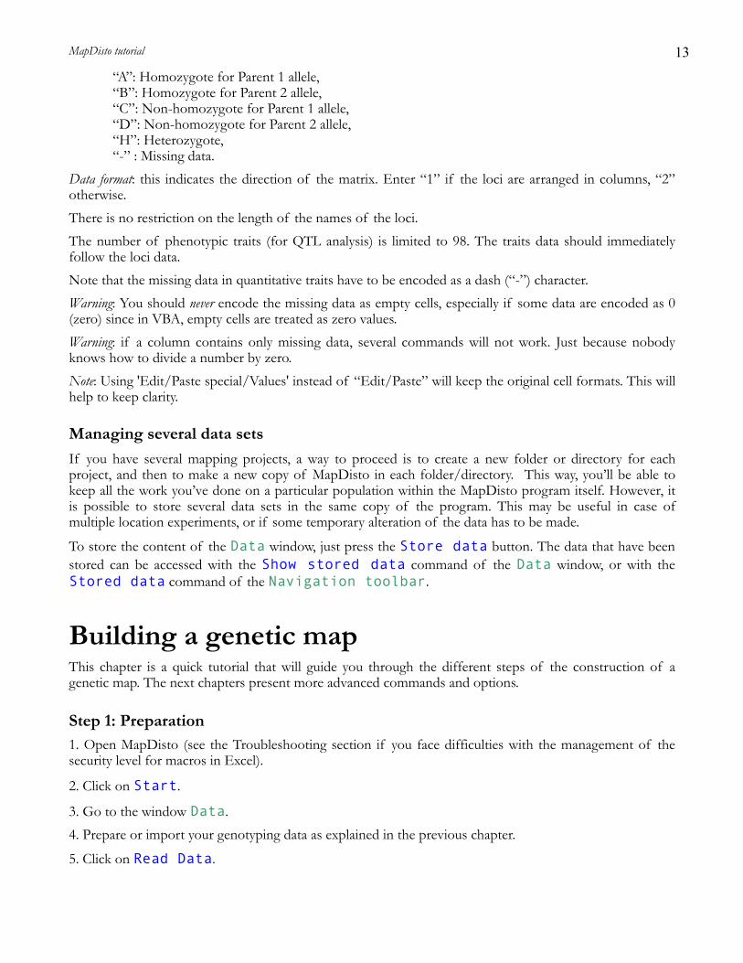
“A”: Homozygote for Parent 1 allele,“B”: Homozygote for Parent 2 allele,“C”: Non-homozygote for Parent 1 allele,“D”: Non-homozygote for Parent 2 allele,“H”: Heterozygote,“-” : Missing data.

Data format: this indicates the direction of the matrix. Enter “1” if the loci are arranged in columns, “2” otherwise.

There is no restriction on the length of the names of the loci.

The number of phenotypic traits (for QTL analysis) is limited to 98. The traits data should immediately follow the loci data.

Note that the missing data in quantitative traits have to be encoded as a dash (“-”) character.

Warning: You should never encode the missing data as empty cells, especially if some data are encoded as 0 (zero) since in VBA, empty cells are treated as zero values.

Warning: if a column contains only missing data, several commands will not work. Just because nobody knows how to divide a number by zero.

Note: Using 'Edit/Paste special/Values' instead of “Edit/Paste” will keep the original cell formats. This will help to keep clarity.

Managing several data sets

If you have several mapping projects, a way to proceed is to create a new folder or directory for each project, and then to make a new copy of MapDisto in each folder/directory. This way, you’ll be able to keep all the work you’ve done on a particular population within the MapDisto program itself. However, it is possible to store several data sets in the same copy of the program. This may be useful in case of multiple location experiments, or if some temporary alteration of the data has to be made.

To store the content of the Data window, just press the Store data button. The data that have been

stored can be accessed with the Show stored data command of the Data window, or with the Stored data command of the Navigation toolbar.

Building a genetic mapThis chapter is a quick tutorial that will guide you through the different steps of the construction of a genetic map. The next chapters present more advanced commands and options.

Step 1: Preparation

1. Open MapDisto (see the Troubleshooting section if you face difficulties with the management of the security level for macros in Excel).

2. Click on Start.

3. Go to the window Data.

4. Prepare or import your genotyping data as explained in the previous chapter.

5. Click on Read Data.

MapDisto tutorial

14

If no message of error is displayed, this should mean that your data are correctly formatted and are ready to be analyzed. Otherwise, the program will try to identify the origin of the problem.

6. Click on Commands.

Step 2: Finding the linkage groups

This steps consists in trying to find a number of linkage groups that equals the number of haploid chromosomes of the species we are working on.

1. Click on Find groups

2. In the Sequence for searching groups dialog box, click on Use all loci

3. In the Find groups dialog box, click on OK without altering the default values for LODmin and rmax.

The program will compute the matrices of two-point recombination fractions and LOD scores for linkage, and will search for linkage groups using the default parameter values. The time required for computing the two-point matrices depends on the number of loci, m, and individuals, n.

Note: The status bar (located to the left below of the window) indicates the progress of the computations for the majority of the commands.

The output of this command consists in sequences, which are series of linked molecular markers.

Validate the sequences with the Add sequences command. Press the Commands button to return to the main window.

You may have to try different values for LODmin and rmax, until you reach the desired number of linkage groups. The quickest way to proceed is to start with less stringent values for LODmin and rmax, then “cut” the large linkage groups that seem to correspond to more than one chromosome using more stringent values. This is done by running again the Find groups command and indicating the number of the

sequence to be “cut” in the Sequence for searching groups dialog box, then using more stringent LODmin and rmax values progressively until reaching the correct number of chromosomes.

Step 3: Ordering the linkage groups

If you are note familiar with the methods for ordering loci, you may want to read first the Annex 1.

In the main window, indicate the number of the sequence of loci you will work with in the Current

working sequence cell.

For short sequences (typically containing less than 10 loci), you can use the Compare all orders command will compute all the possible maps and thus will lead to the best map with certainty, according to the chose criteria (in our case, the SARF).

For longer sequences, it is necessary to use an alternative method, as the former would take a too long time (see Annex 1). Click on Order sequence. This command implements one of the three following algorithms: Seriation, Branch & Bound II, Unidirectional Growth. For this tutorial, just choose Seriation

method in Options… / Method for Ordering loci. Several criteria are available for the

seriation method, select SARF (Sum of Adjacent Recombination Frequencies) in Options… /

Criteria for Ordering and Ripple.

Use the AutoOrder command to apply the Order sequence to all declared sequences in a single step.

MapDisto tutorial

15

Step 4: Refining the order

For the sequences that were orderd using the Order sequence command, use the Ripple order

and Check inversions commands to try to locally improve the mapping result.

Use the AutoRipple and AutoCheckInversions commands to apply the Ripple ordert and the CheckInversions to alllared sequences in a single step.

Step 5: Displaying the map

Click on Draw all sequences to draw a graphical representation of the computed maps of all the declared sequences.

In Options…, play with the different parameters of the Draw map section.

Advanced mapping operationsThe methods described in this chapter relate to validation and verification steps of the maps obtained in the previous chapter.

Verifying Mendelian segregation

Use Segregation !2s to obtain chi-squared values that will test for Medelian segregation of the indicated sequence.

What is the meaning of a significant !2 value?

What to do with loci that show non-Mendelian segregation?

The command also computes deviations from 1:3 and 3:1 segregations. This feature can be useful for dominant markers such as AFLPs or RAPDs, when two bands have very similar sizes and cannot be separated on the gel. The apparent band then segregates (1 absent:3 present), and has no unique location on the map.

Visualize map details

The Detailed map command will show more details than Draw a sequence command. The computed parameters are: classical or corrected recombination fractions, map distances and their associated standard deviations, linkage and independence khi2s, LOD scores and population size for each interval.

Why is the sr parameter important?

Checking for order solidity

A nice way of evaluating the stability or robustness of a given order is to use resampling methods. Choose a sequence and click on Boostrap order (with, for example, 500 trials).

Interpret the results in terms of stability of the order estimation.

How does affect the robustness of the map order?

MapDisto tutorial

16

The Three point… commands is another way to verify the stability of the obtained order. It tests for differences in likelihoods of all possible maps constitued by permutations of triplets od adjacent loci. I personnaly prefer the boostrapping method, which I find more intuitive and easier to understand.

Identifying problematic loci

The Drop locus command drops one locus at a time for a specific sequence and re-computes the map. Output gives pairwise distances (cM) between the remaining markers after each one is dropped. Full map is the last column.

A locus that causes an important negative difference in the map size is expected to contain erroneous data and should be removed of the analysis process. Note that dropping the terminal markers can have a large effect on map order simply because they are loosely linked. Also, if a sequence of markers are loosely linked, then it is inevitable that dropping one will have a large effect on the map.

Note: this command complements well Boostrap order, it’s recommended to use both in order to identify a set of markers that will constitute a solid framework for the map.

Identifying genotyping errors

A way to identify potential gentyping errors is to look at double recombinants, or singletons. This is the

purpose of the Color genotypes window. In the main windowclick on Color genotypes

Click on Load data, then Color, then Show double recombinants

Use the Show error candidates command, playing with the Threshold for error

detection parameter.

Dealing with segregation distortion

Several options are available in the Options...: Classical, Bailey, Custom. In the case of Backcross, Single Seed Descent or SSD, Doubled Haploid or DH populations, various recombination fractions estimates may be computed: the classical one, Bailey's estimate (Bailey 1949) and a Custom estimate that

handles for selection against any genotypic class of the progeny. Please read the Help section (built-in in the program itself) for more details.

Note: These options do not apply to F2 populations.

Comparing a computed genetic map to a reference mapWe will take the example of rice (O. sativa L.), in order to show how to compare the map you have obtained with MapDisto to the physical map known from the complete sequencing data available.

Load the Rice_Data.xls file (available from the author). Follow all the steps of the previous chapters to and make sure that all linkage groups have been properly ordered.

In the main window, click on Define as Map 1.

Back to the main window, click on Extract map from DB….

MapDisto tutorial

17

Click on Load marker list, then Extract positions…. Locate the folder that contains

DB_Rice_Markers.xls the file (available from the author). Click on Open. Visualize loci position on the physical map using the Draw map command.

Clcik on Back, then Define as Map 2. This will re-compute your genetic map based on the order of the defined sequences and will get you to the Compare Maps window.

Click on Compare maps.

Do you observe inversions of loci orders between the two maps?

Observe how the bp/cM ratio changes along the chromosomes.

Assessing the effect of erroneous data fraction using simulationsThrough this simulation experiment, we will see how the map size expands due to erroneous data.

In the main window, click on Clear all results, then Clear sequences, then

Simulations….

Simulate a map using the Simulate a map command, with two chromosomes, an average density of

1 cM and a total size of 200 cM. Visualize the map using Draw map.

Click on Add to My sequences to add the linkage groups to My sequences.

Simulate a BC1 population using Simulate a population, with 100 individuals and a random error rate of 0%.

Click on Use these data. The program will prompt to ask if you want to store the data currently in

use. Cleak on Read data, then Commands, then Draw all sequences.

Note the total size of the map.

Simulate new populations, in changing gradually the error rate (e.g., from 0.01 to 0.1)

Observe how map size inflates when error rate is set to different values.

Use the tools available in the Color!genotypes window to detect and remove erroneous data.

Use Compare maps… to compare the maps with and without error data.

Looking for QTL locations[To be completed...]

MapDisto tutorial

18

Exporting a map created in MapDisto for QTL analysis programs[To be completed...]

Exporting data for Mapmaker/EXP[To be completed...]

Importing a map created in another program[To be completed...]

MapDisto tutorial

19

Command reference

Commands in the main menu window

Find groups Finds linkage groups in the specified sequence.

Compare all orders This command is useful for ordering loci in small sequences. It compares a user-defined criteria for all possible orders in the declared sequence and displays the 20 smaller orders. Three criteria are available: SARF, or Sum of Adjacent (two-point) Recombination Fractions, Log(L) that is the sum of the log-likelihoods for each adjacent pair of loci, or SAD that is the Sum of Adjacent Distances in centimorgans (In the Criteria for ordering loci section of the Options). I usually use SARF, as, assuming that if there are not too many missing data, the smallest order should not be so far to the "true" order.

Order sequence This command tries to find the best order in long sequences. As it is very time and memory consuming to investigate all possible orders with large numbers of loci, the algorithm used here is a heuristic. This means that it does not provide the best order (according to the chosen criteria) with certainty. However, it should always give an order that is close to the best one. The SARF, Log(L) and SAD criteria may be chosen.

Ripple order Use it to verify local orders in a long sequence (typically, after the "Order sequence" command). It will slide a window of five loci and compute the 120 possible maps for each window. The SARF, Log(L) and SAD criteria may be chosen.

Drop locus For a specific sequence (linkage group), this command drops the loci one by one and computes the corresponding map. It is useful to quickly identify the loci that present bad quality data. Typically, a strong negative difference in map size after removing a locus indicates the presence of bad data for this locus.

Boostrap order Use it to verify an order and detect "weak points" in a linkage group map. This command lets the user to implement Bootstrap and/or Monte Carlo procedures to estimate and verify a sequence order. To choose the Bootstrap procedure only, don't check the "Reshuffle initial order" check box in the dialog box when you are prompted for Bootstap parameters. To choose the Monte Carlo procedure only, check the "Reshuffle initial order" check box and enter the value "100" in the field "Subsample size". To perform a combined test (Bootstrap + Monte Carlo at the same time), check the "Reshuffle initial order" check box and choose a value of Subsample size inferior to 100

AutoOrder automatically orders all the declared sequences in the "My sequences" section of the Main menu. For long sequences (more than six loci), this procedure uses the "Order sequence algorithm. For sequences made of two to six loci, it uses the "Compare all orders" algorithm.

AutoMap Runs successively the "Find groups", "AutoOrder" and "Draw all sequences", to allow for a very easy and quick display of the map computed for all the loci declared in the Data window. Try it!

Detailed map Computes the map of a specified sequence. The computed parameters are: r.f., map distances, linkage and independance khi2s, LOD scores and population size for all intervals. You have to declare a locus order (the sequence) and a r.f. estimate (classical, Bailey, customised).

Segregation !2s Computes segregation chi-squared tests (which measure the deviation from a 1:1 segregation) and their associated probabilities for a particular sequence. It also computes deviations from 1:3 and 3:1 segregations. This feature can be useful for dominant markers such as AFLPs or RAPDs, when two bands have very similar sizes and cannot be separated on the gel. The apparent band segregates (1 absent : 3present), and has no unique location on the map.

MapDisto tutorial

20

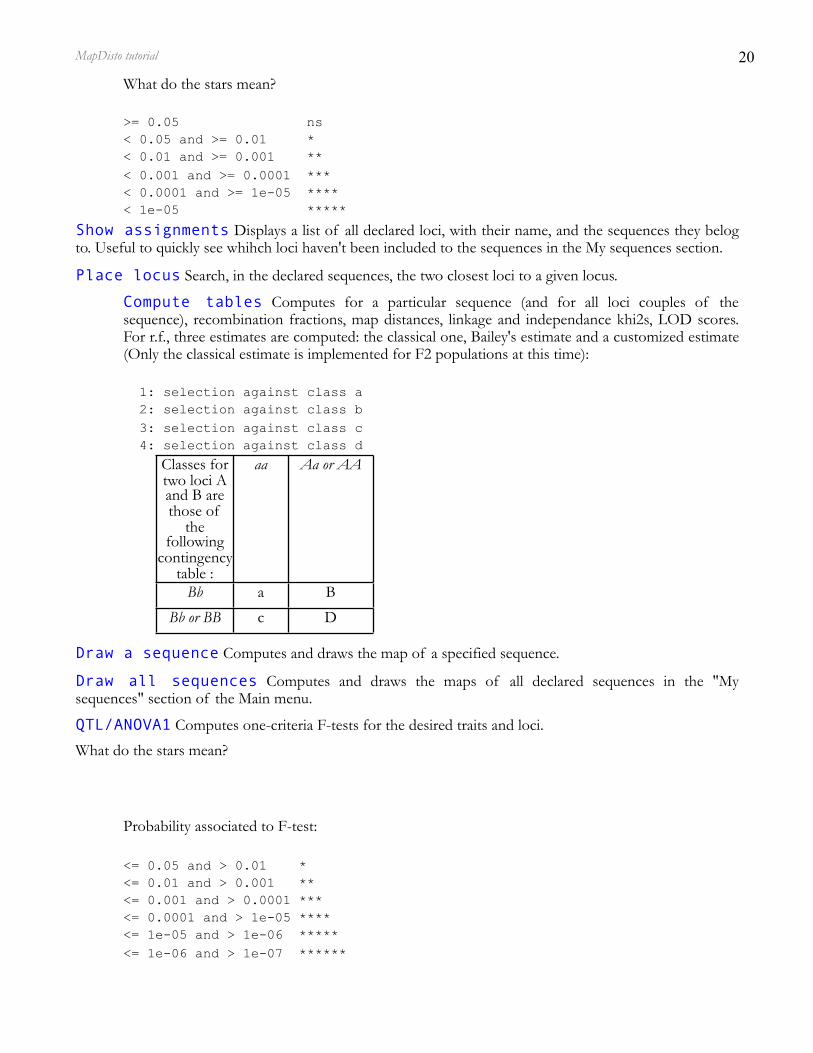
What do the stars mean?

>= 0.05 ns

< 0.05 and >= 0.01 *

< 0.01 and >= 0.001 **

< 0.001 and >= 0.0001 ***

< 0.0001 and >= 1e-05 ****

< 1e-05 *****

Show assignments Displays a list of all declared loci, with their name, and the sequences they belog to. Useful to quickly see whihch loci haven't been included to the sequences in the My sequences section.

Place locus Search, in the declared sequences, the two closest loci to a given locus.

Compute tables Computes for a particular sequence (and for all loci couples of the sequence), recombination fractions, map distances, linkage and independance khi2s, LOD scores. For r.f., three estimates are computed: the classical one, Bailey's estimate and a customized estimate (Only the classical estimate is implemented for F2 populations at this time):

1: selection against class a

2: selection against class b

3: selection against class c

4: selection against class d

Classes for two loci A and B are those of

the following

contingency table :

aa Aa or AA

Bb a B

Bb or BB c D

Draw a sequence Computes and draws the map of a specified sequence.

Draw all sequences Computes and draws the maps of all declared sequences in the "My sequences" section of the Main menu.

QTL/ANOVA1 Computes one-criteria F-tests for the desired traits and loci.

What do the stars mean?

Probability associated to F-test:

<= 0.05 and > 0.01 *

<= 0.01 and > 0.001 **

<= 0.001 and > 0.0001 ***

<= 0.0001 and > 1e-05 ****

<= 1e-05 and > 1e-06 *****

<= 1e-06 and > 1e-07 ******

MapDisto tutorial

21

<= 1e-07 and > 1e-08 *******

<= 1e-08 and > 1e-09 ********

<= 1e-09 and > 1e-10 *********

<= 1e-10 and > 1e-11 **********

<= 1e-11 and > 1e-12 ***********

<= 1e-12 and > 1e-13 ************

<= 1e-13 and > 1e-14 *************

<= 1e-14 and > 1e-15 **************

<= 1e-15 and > 1e-20 ***************

<= 1e-20 and > 1e-25 ****************

<= 1e-25 and > 1e-50 *****************

<= 1e-50 ******************

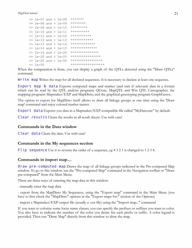
When the computation is done, you can display a graph of the QTLs detected using the "Draw QTLs" command.

Write map Writes the map for all declared sequences. It is necessary to declare at least one sequence.

Export map & data Exports computed maps and marker (and trait if relevant) data in a format which can be read by the QTL analysis programs QGene, MapQTL and Win QTL Cartographer, the mapping programs Mapmaker/EXP and MapDisto, and the graphical genotyping program GraphGenot.

The option to export for MapDisto itself allows to draw all linkage groups at one time using the 'Draw map' command and enjoy colored marker names.

Export data Exports you data in a Mapmaker/EXP-compatible file called "MyData.raw" by default.

Clear results Clears the results in all result sheets. Use with care!

Commands in the Data window

Clear data Clears the data. Use with care!

Commands in the My sequences section

Flip sequence Use it to reverse the order of a sequence, eg 4 3 2 1 is changed to 1 2 3 4.

Commands in import map…

Draw pre-computed map Draws the map of all linkage groups indicated in the Pre-computed Map window. To go to this window, use the "Pre-computed Map" command in the Navigation toolbar or "Draw pre-computed" from the Main Menu.

There are three ways of entering the map data in this window:

- manually enter the map data

- export from the MapDisto My Sequences, using the "Export map" command in the Main Menu (you have to first check the "MapDisto" options in the "Export maps for:" section of the Options)

- import a Mapmaker/EXP output file (usually a .out file) using the "Import map..." command

If you want to colorize some locus name classes, you can specify the prefixes or suffixes you want to color. You also have to indicate the number of the color you desire for each prefix or suffix. A color legend is provided. Then run "Draw Map" directly from this window to draw the map.

MapDisto tutorial

22

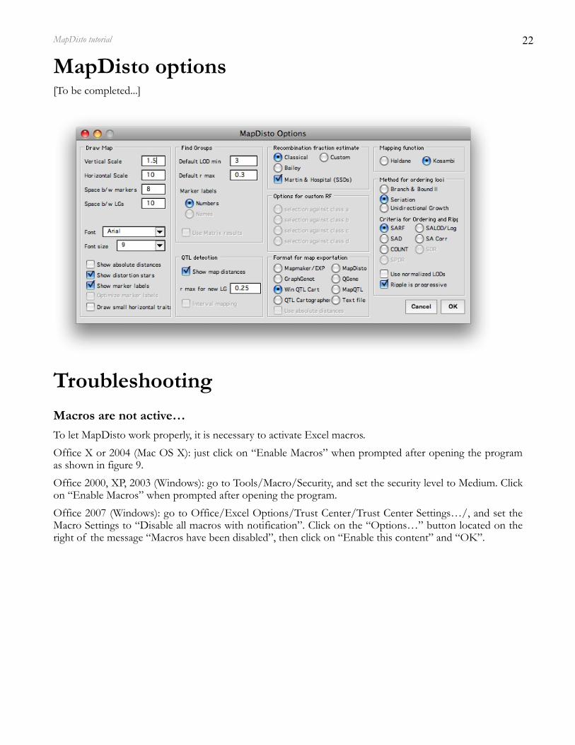
MapDisto options[To be completed...]

Troubleshooting

Macros are not active…

To let MapDisto work properly, it is necessary to activate Excel macros.

Office X or 2004 (Mac OS X): just click on “Enable Macros” when prompted after opening the program as shown in figure 9.

Office 2000, XP, 2003 (Windows): go to Tools/Macro/Security, and set the security level to Medium. Click on “Enable Macros” when prompted after opening the program.

Office 2007 (Windows): go to Office/Excel Options/Trust Center/Trust Center Settings…/, and set the Macro Settings to “Disable all macros with notification”. Click on the “Options…” button located on the right of the message “Macros have been disabled”, then click on “Enable this content” and “OK”.

MapDisto tutorial

23

Figure 9. Prompt window for Macros activation in Excel 2004.

The program generates errors when I modify some parameters…

Some minor problems may occur with localized versions of Excel, especially for those languages that use a comma to separate the decimals (e.g., French or Spanish). This may be fixed in altering the settings of the operating system (For Windows systems, this has to be in Control Panel/Numbers). I have not noticed any problem with French Excel versions running on Mac OS X.

MapDisto tutorial

24

Annex 1: Methods for ordering lociTo find the correct order of the loci that make the linkages groups is the most difficult step of the construction of a genetic map.

We won’t go here into the details of these algorithms, but it is important to know that two main families of methods for estimating a map have been developed. We are talking here of estimating the recombination fractions between the loci, assuming a given order. The first algorithm is based on two-point estimates, and the second one is based on multipoint estimates. Historically, the multipoint methods were designed for human genetics, to deal with the problem of finding the order of several loci that do not segregate in the same families that constitute the mapping population (Lathrop et al, Lander et all, Ott et all). For experimental populations, like backcross, intercross, recombinant inbreds etc., the advantage of the multipoint approaches is less evident, as, in the case of “perfect” data!– i.e., no missing data, no genotyping error!-, the two-point estimates are equivalent to the multipoint ones.

Besides, and independently from the method for estimating the map, one have to use an algorithm that will find the order of the loci.

The first and obvious algorithm is to compute all the possible maps for a given sequence. This is the best possible method, as it provides with certainty the best map according to the chosen criteria. Unfortunately, we will probably have to wait for a long time before we see a computer that is able to run this algorithm for dense maps, i.e. with several dozens of markers per chromosome. Indeed, given a sequence of m markers, then number of possible orders is m!/2. This means that a sequence of 10 loci has 1,814,400 possible orders. With the current processors on the marker, to compute all the possible maps will take between 10 mn and one hour, depending on the computing method, the programming language and some other parameters. Now, just consider a sequence with 20 loci: there are 1.22 x 1018 map orders and it would take approximately 65 million years to compute all of them... A sequence with 100 loci (which is becoming common) has 4.66 x 10157 possible maps and the time required to compute all possible maps is not even comparable to the age of the Universe.

Thus, the only way to infer the correct order of dense maps is to imagine heuristics. A heuristic is an algorithm that tries to reach a fairly good solution (if not the best) to a problem without computing all the possible situations. Many algorithms have been proposed to reach the best order (see Tan and Fu 2006 for a review).

MapDisto proposes uses two original heuristics for ordering loci. However, I realized that these algorithms are quite close to already published methods, and this is why I called them seriation!II and branch and bound!II, to refer to the already published seriation (Buetow and Chakravarti 1987) and branch and bound (Lathrop et al. 1985) algorithms.

Moreover, I have implemented the unidirectional growth algorithm (Tan and Fu 2006) as it seems to have good statistical properties.

I have found the seriation II and branch and bound II algorithms to generally give very good results. The universal growth algorithm may performs well also, however, its main weakness resides in the fact that its performance level is closely related to its ability to find the right starting map, which I have found to be failing a number of times using real data sets.

The universal growth algorithm uses its own criteria to look for the best map. The goal of this method is basically to look for the shortest map. In the seriation II and the branch and bound II algorithm, one have to choose the criteria for deciding which is the best map. In MapDisto, the proposed criteria are:

-!SARF, or Sum of Adjacent Recombination Frequencies,

-!SALOD/Log(L), or Sum of Adjacent LOD scores,

MapDisto tutorial

25

-!SAD, or Sum of Adjacent Distances, where the distance is the recombination frequencie converted to a map distance using the Haldane or the Kosambi mapping function,

-!SA Corr, or Sum of Adjacent Correlations, where the correlation is a combination of the recombination fraction and the LOD score:

Corr = 1! r( ) 1! e!LOD( ) .

-!COUNT, or sum of observed recombination events.

MapDisto tutorial

26

References[To be completed]

Bailey NTJ (1949) The estimation of linkage with differential viability, II and III. Heredity 3:220-228

Bailey NTJ (1951) Testing the solubility of maximum likelihood equations in the routine application of scoring methods. Biometrics 7:268-274

Buetow, K. N., and A. Chakravarti, 1987 Multipoint gene mapping using seriation. Am. J. Hum. Genet. 41: 189–201.

Kosambi D.D. 1944. The estimation of map distance from recombination values. Ann. Eug. 12: 172-175.

Lathrop, G. M., J. M. Lalouel, C. Julier and J. Ott, 1985 Multilocus linkage analysis in humans: detection of linkage and estimation of recombination. Am. J. Hum. Genet. 37: 482–498. Lorieux M., B. Goffinet, X. Perrier, D. González de León & C. Lanaud. 1995. Maximum-likelihood models for mapping genetic markers showing segregation distortion. 1. Backcross populations. Theoretical and Applied Genetics 90:!73-80.

Lorieux M., X. Perrier, B. Goffinet, C. Lanaud & D. González de León. 1995. Maximum-likelihood models for mapping genetic markers showing segregation distortion. 2. F2 populations. Theoretical and Applied Genetics 90:!81-89.

Tan YD and Fu YX (2006) A Novel Method for Estimating Linkage Maps. Genetics 173: 2383–2390

MapDisto tutorial