managing the uk national debt...
TRANSCRIPT
Managing the UK National Debt 1694-2017∗
Martin Ellison† Andrew Scott‡
September 2017
Abstract
We construct a new monthly dataset for UK government debt over the period 1694 to 2017 based
on price and quantity data for each individual bond issued. This enables us to examine long run fiscal
sustainability using the theoretically relevant variable of the market value of debt, and investigate the
historical importance of debt management. We find the general implications of the tax smoothing literature
are replicated in our data, especially around financing wars, although we find major shifts over time in how
fiscal sustainability is achieved. Before the 20th century, governments continued to pay bond holders a
high rate of return and achieved sustainability through running fiscal surpluses but since then governments
have relied on low growth adjusted real interest rates. The optimal debt management literature tends
to favour the use of long bonds but we find the government would have been better off over the 20th
century issuing short bonds. The contrast with the literature occurs because of an upward sloping yield
curve and long bonds rarely providing fiscal insurance. This is particularly true during periods of financial
crises when falling interest rates lead to sharp rises in the price of long bonds, making them an expensive
form of finance. We examine the robustness of our conclusions to liquidity effects, rollover risks, buyback
operations and leverage. In general, these do suggest a greater role for long bonds but do not overturn an
issuance strategy based mainly on short term bonds.
JEL Classification : E43, E62, H63
Keywords : Debt Management, Fiscal Deficits, Fiscal Policy, Government Debt, Inflation,
Maturity, Yield Curve
∗We thank Bill Allen, Paul Beaudry, Francis Breedon, Forrest Capie, Nick Crafts, George Hall, Eric Leeper, Albert Marcet,
Paul Marsh, Larry Neal, Kevin O’Rourke, Tom Sargent and participants at the 2nd Oxford - Federal Reserve Bank of New
York Monetary Economics Conference, the National Institute for Economic and Social Research, Oxford University Economic
History seminar, the Royal Economic Society Conference 2017 and Universitat Autonoma de Barcelona for helpful comments
and suggestions. Giorgia Palladini, William Hesselmann and Kay Ellison provided excellent research assistance. Martin Ellison
acknowledges support from the European Research Council under the EU 7th Framework Programme (FP/2007-2013), Advanced
Grant Agreement No. 324048 (PI Albert Marcet).†University of Oxford and CEPR‡London Business School and CEPR
1

1 Introduction
Managing the national debt is a key economic challenge for any government and requires answering two peren-
nial questions: what is the appropriate level of government debt? and what type of debt should governments
issue?
The theory informing the right level of national debt starts from the implication of the government’s
intertemporal budget constraint that the market value of government debt has to be matched by the net
present value of future primary surpluses. If we add the assumptions of distortionary taxes, no default and
incomplete markets then the prescription is that the national debt should follow a random walk, as shown by
Aiyagari et al (2002). In other words, there is no specific right level for the national debt other than limits
aimed at ruling out Ponzi schemes.1 The implication of this was noted already by Adam Smith (1776), “Great
Britain seems to support with ease a debt burden which, half a century ago, nobody believed her capable of
supporting”.2
In terms of what type of debt governments should issue, a growing consensus has emerged that long bonds
provide considerable advantages (Angeletos (2002), Barro (2003), Nosbusch (2008), Lustig, Sleet and Yeltekin
(2009)). If the market value of long bonds falls when there are adverse persistent government expenditure
shocks then long bonds provide the government with a form of “fiscal insurance”. The negative covariance
between market values and expenditure shocks means, through the intertemporal budget constraint, that taxes
have to rise by less than otherwise and hence long bonds are appealing. However, these advantages of long
bonds are not uncontested. Buera and Nicolini (2004) and Faraglia el al (2010) show that exploiting the
fiscal insurance properties of long bonds requires the government to take portfolio positions that are extreme,
volatile and potentially unstable, whilst Faraglia et al (2017) show how the advantages of long bonds are much
reduced when allowance is made for the reluctance of governments to buyback debt each period.
This paper seeks to provide insight on managing the national debt and answers to the two key questions
by utilising new empirical evidence. On the basis of archival research at the Bank of England and the British
Library, we construct a new and detailed database showing how the UK national debt has been managed in
practice from 1694 to 2017. Key to this dataset is the fact that it is built up from monthly price and quantity
data based on each individual bond issued by the government. The breadth and granularity of our data provides
two major advantages. The first is that it enables us to examine over 323 years the theoretically relevant concept
of the market value of government debt rather than the more commonly used amount outstanding. Given our
dataset includes upwards of 60 business cycles, 6 major wars and 6 major financial crises, it provides a rich
understanding of how fiscal policy has operated across a range of different macroeconomic contexts. The second
advantage of our dataset is that its gilt-by-gilt foundations allows us to empirically examine the contribution
of debt management towards achieving fiscal sustainability. By performing historical decompositions and
counterfactuals, our dataset enables an assessment of a number of claims made in the optimal tax and debt
management literatures and provide insight into observed debt management.
The paper is organised as follows. In Section 2 we outline our dataset and how it is constructed. We
1See Reinhart and Rogoff (2009) for a recent empirically-based analysis documenting apparent debt ceilings2The historian Macauley (1899) is even more forthright “At every stage in the growth of debt it has been seriously asserted
by wise men that bankruptcy and ruin were at hand. Yet still the debt went on growing, and still bankruptcy and ruin were as
remote as ever”.
2
provide a detailed narrative of UK public finances over this period highlighting a number of features about
debt structure and management. Key to our analysis is the use of holding period returns to calculate the cost
of government funding. Therefore Section 3 derives zero coupon yield curves and calculates the total holding
returns for the universe of bonds issued, taking into account both coupon payments and revaluations. Section
4 turns to understanding debt dynamics and the role of macroeconomic variables and debt management in
achieving fiscal sustainability over the whole sample period, various sub-samples and specific episodes such as
wars and financial crises. In Section 5 we utilise the gilt-by-gilt nature of our dataset and consider alternative
debt management policies, performing ex post counterfactuals to assess their performance relative to actual
outcomes. Whilst the optimal debt management literature tends to favour the use of long bonds, we find in
our dataset that relying on short bonds would have led to better out-turns. However, focusing solely on short
term bonds raises a number of risks and concerns that tend to occupy actual debt management operations. In
Section 6 we extend our analysis to consider whether our findings are robust to issues of liquidity and price
shifts, rollover risks, leverage and buybacks. We find that whilst some of these factors, especially rollover risk,
do introduce a greater role for long term bonds, it is still the case that an issuance strategy based on a majority
of short term bonds is found ex post to outperform issuance of longer bonds. A final section concludes.
2 UK Government Debt 1694-2017
The starting date for UK government debt is widely seen as 1694 when King William III used a syndicate of
merchants to sell debt to finance the Nine Years’War.3 This syndicate went on to become the Bank of England
and so data on the level of UK government debt is available from this date onwards.4 The government did
borrow before 1694 but mainly made use of tallies, effectively bills backed up by specific taxes or excise duties
falling due over short term horizons. The year 1694 is widely seen as marking the beginning of the institutional
framework for government debt which supported the growth of the British economy and ultimately the British
empire (Brewer (1989)), although debt issuance in the early years was understandably developmental.5 Many
of the initial loans took an unconventional form by current standards, including annuities and lotteries as
parts of their design, but alongside these were a number of perpetual bonds offering different coupon rates. By
1752 these perpetual bonds were consolidated (“consols”) in a smaller number of distinct stocks offering fixed
coupon payments and the bond market took a more recognisably modern form. However, it was not until the
early 20th century that finite dated long bonds were issued6 , marketable debt in the 18th and 19th century
consisting entirely of perpetuals/consuls and short term bills.
3Technically the debt only became UK debt when the United Kingdom was created by the Act of Union in 1707 which joined
together the Kingdoms of England and Scotland.4http://www.ukpublicspending.co.uk/debt_history. The initial loan from the Bank of England was for £ 1.2million at an 8%
interest rate and with a £ 4,000 management fee. It has now been repaid.5See Dickson (1967) for a comprehensive history and detailed account of the development of the UK government debt market
in the aftermath of the Glorious Revolution of 1688.6The first fixed term gilt in our sample period (4.5% War Loan 1925-45) was issued November 1914.
3

2.1 Quantities
We use data on the quantity of UK government debt for each gilt7 outstanding from the Return relating to
the National Debt which is presented annually to the House of Commons by the Financial Secretary to the
Treasury, the gilt sheets produced by the broker Mullins and, for more recent periods, the Heriot-Watt British
Government Securities Database. Since 27th March 1981 the UK government has also issued indexed-linked
debt (bonds indexed to the price level) and by July 2017 the stock of indexed gilts had risen to represent about
one quarter of the total value of debt.
1700 1750 1800 1850 1900 1950 2000
Deb
tto
GD
P ra
tio
0
100
200
300Total debtMarketable debt
Figure 1: Face value of total and marketable debt as a percentage of GDP
Figure 1 shows the face value of outstanding marketable debt relative to GDP from 1700 to 2016 as
constructed by our gilt-by-gilt approach. For comparison we also show the total value of all debt outstanding
from the Bank of England’s A Millennium of Macreconomic Data database. GDP data is from the Bank
of England database, taken from Mitchell (1988) for 1700-1954 and the Offi ce for National Statistics website
from 1955 onwards. Gilts represent only the marketable component of government debt and to varying degrees
the government has also made use of non-marketable debt. A major source of nonmarketable debt have been
sizeable international loans, especially from the US government during WWI and WWII (eventually repaid in
2006). Currently the main forms of outstanding non-marketable debt are a range of retail savings products
sold by the National Savings Authority, such as premium bonds (a form of lottery) and investment accounts.
The series for total debt in Figure 1 generally shows the same swings and oscillations as that for marketable
debt. In the early years of our sample loans and annuities were the main component of overall debt, but as the
market developed during the 18th century the amount of non-marketable debt declined. However, WWI and
WWII required a large increase in debt and a substantial amount was in non-marketable form (War Loans)
such that by 1947 the debt mix was more 50-50. Subsequent repayment of those loans and some partial default
nevertheless rendered most of the government debt again marketable by the end of our sample period.
The overall path of the debt to GDP ratio is well known and reflects the twists and turns of British
history. The 1700s sees a series of wars with only brief periods of peace and reductions in debt. Wars became
increasingly expensive and led to ever higher levels of debt, peaking with the end of the Napoleonic Wars in
1815 and then beginning a long term decline. Debt then experiences a large increase because of WWI; further
increases in the 20s due to weak growth; a further jump because of WWII; a long period of decline after WWII
7UK government bonds are called “gilts” as originally purchasing the bond meant receiving a gilt edged security as proof of
purchase.
4

until the late 90s (with various cyclical fluctuations) and then from the late 90s a flattening of the trend and
signs of a modest increase before a sharper rise and higher trend in the wake of the 2007/8 Global Financial
Crisis. Debt rises sharply after the 2007/8 Financial Crisis, reaching above 100% of GDP but ending the
sample slightly below the average for the entire period.8
The fluctuations in Figure 1 reflect only issuance and redemptions over time because the UK government
has never formally defaulted on any of its marketable debt. There are though a number of “conversions”in our
dataset. UK gilts were redeemable by the government when their value rose above par, so on several occasions
the government used this as an opportunity to retire gilts paying a high coupon and reissue gilts paying a
lower coupon. This process was called a “conversion”and was often used to reduce the interest payments on
debt. Anyone not wishing to switch to the lower coupon bond received payment at par. Reinhart and Rogoff
(2009) classify one such conversion (the conversion in 1932 of the 1917 War Loan which had been callable since
1929 and was converted from a 5% to a 3.5% stock) as a default but regardless of how we classify this issue
our dataset reflects the change - it counts as retirement of an existing bond and the re-issuance of a new one.
The case of non-marketable debt is more complicated, especially regarding US loans. There was an outright
default on some WWI loans from the US, connected to Germany’s own debt default to the UK, as well as
various incidents of suspension of payments and changes to the payment profile for the WWII loans. Our focus
is however solely on marketable debt so these issues do not impact upon our analysis.
The long sweep of more than 300 years of data in our sample is ideal for considering the long run properties
of debt. Whether or not debt possesses a unit root and its persistence relative to other macroeconomic variables
has been a mainstay of the tax smoothing literature. Figure 2 plots Cochrane’s (1988) measure of persistence
for debt, GDP, government expenditure and the primary surplus in our data. This measure is defined as
(1/k)V ar(yt − yt−k) and tends to 0 if a variable is made up of purely stationary components, tends to 1 if it
is a unit root, and is greater than 1 if it shows greater than unit root persistence. Figure 2 confirms the Barro
(1979) and Aiyagari et al (2002) finding that debt shows unit root persistence and the Marcet and Scott (2009)
observation that debt shows more persistence than any other variable. This is consistent with the notion of
debt playing a buffer role in absorbing large temporary expenditure shocks, and implies that bond markets do
not provide the insurance that a complete market paradigm would suggest.9 In other words, over the last 323
years it is debt that has been the main mechanism absorbing fiscal shocks.
8For insightful and detailed analysis of UK government debt management over this sample period see Dickson (1967) for
1688-1756, O’Brien (2008) for 1756 to 1815, Clark (2001) for 1727-1840 and Allen (2012) for 1919 onwards.9Although our debt and GDP terms show similar levels of persistence, note that the debt term is debt to GDP so debt contains
an additional unit root component over and above that in GDP.
5

k0 5 10 15 20
V(k)
0
0.5
1
1.5
2debt/GDPlog real GDPlog real Gprimary surplus/GDP
Figure 2: Persistence of debt, GDP, government spending and the primary surplus
2.2 Instruments
Whilst the debt management literature tends to focus on the relative merits of short versus long run bonds,
hardly any attention is given to the actual number of bonds a government issues, something our dataset
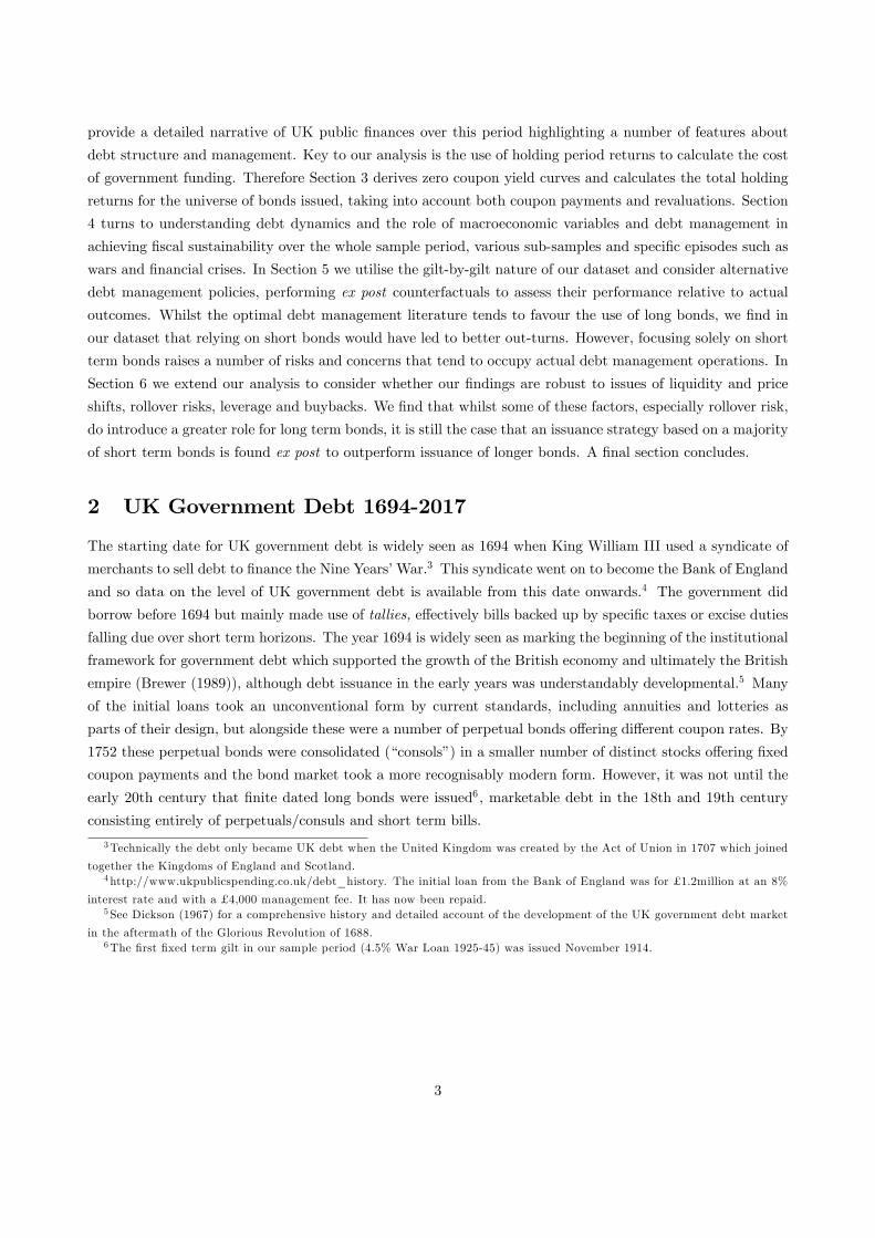
enables us to document. Figure 3(a) shows a time plot of the number of distinct10 gilts outstanding at any
point in time. As previously noted, the early years of UK government debt saw a number of different borrowing
instruments which were eventually simplified with the introduction of consols. By the period 1879-1914 the
debt structure was very simple, with at most only seven different types of gilts being traded in financial markets
on any given date.11 Debt issuance for 1914-1948 was dominated by the need to finance and repay spending
in WWI. This led to a sharp rise in the size of government debt, a greater use of non-marketable debt, and a
sharp increase in the number of distinct bonds issued. By 1939 there were 30 different types of gilts circulating
in financial markets. After 1948, even though the main trend is for debt to decline relative to GDP, there is
an increase in the number of bonds outstanding as the government begins to fill the maturity structure by
issuing more short and medium term bonds. Indexed bonds were first issued in March 1981, which represents
the approximate peak in terms of number of distinct bonds outstanding at more than 100.
Figure 3(b) shows the number of new gilts issued and retired each year, confirming that the government
chose to increase the number of distinct types of gilts available for most periods in the twentieth century. Figure
3(c) shows that the average size of each distinct gilt (as a percentage of GDP) has shown a near continuous
decline over our sample period, except at the end where it slightly increases.12 The increase in the number
of gilts issued is not then simply a result of fluctuations in the level of debt, but a change in behaviour by
government debt managers.13
10A gilt is distinguished by its date of original issuance, its original maturity and its stated coupon rate, e.g., if a twenty year
gilt were issued in 1953 and a ten year gilt in 1963 then in 1963 these would count as two distinct gilts, despite them both having
ten years remaining to maturity. In some instances the government would “top up”previous issues of gilts and we do not count
these top ups as distinct.11Consols were first issued in 1752 and last issued when Winston Churchill was Chancellor in 1927. They were finally redeemed
by the UK government in 2015. At that time the UK Debt Management Offi ce investigated whether there was demand for new
issuance of undated bonds at the time, but found no investor support.12This is due to the retirement of Consols, which were the oldest vintage of government bonds and were relatively small in size
compared to modern day issuance. The retirement of Consols also explains why the number of bonds retired shows a sharp rise
towards the end of Figure 2b.13There are numerous potential explanations for this, e.g., exploiting the whole of the yield curve in order to improve debt
6
1700 1750 1800 1850 1900 1950 20000
50
100
(a) Number of gilts outstanding
1700 1750 1800 1850 1900 1950 20000
10
20(b) Number of gilts issued and retired
IssuedRetired
1700 1750 1800 1850 1900 1950 20000
0.1
0.2(c) Average size of each outstanding gilt relative to GDP
Figure 3: Debt instruments
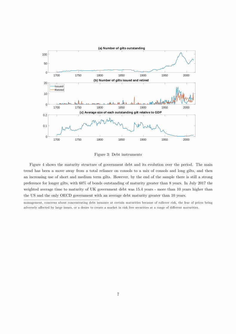
Figure 4 shows the maturity structure of government debt and its evolution over the period. The main
trend has been a move away from a total reliance on consols to a mix of consols and long gilts, and then
an increasing use of short and medium term gilts. However, by the end of the sample there is still a strong
preference for longer gilts, with 60% of bonds outstanding of maturity greater than 8 years. In July 2017 the
weighted average time to maturity of UK government debt was 15.4 years - more than 10 years higher than
the US and the only OECD government with an average debt maturity greater than 10 years.
management, concerns about concentrating debt issuance at certain maturities because of rollover risk, the fear of prices being
adversely affected by large issues, or a desire to create a market in risk free securities at a range of different maturities.
7
1900 1920 1940 1960 1980 2000 2020
Sha
re
0
0.1
0.2
0.3
0.4
0.5
0.6
0.7
0.8
0.9
1
< 1 year Ultra short < 3 years Short 37 years Medium 815 years Long > 15 years Consols
Figure 4: Percentage composition of UK government debt by maturity
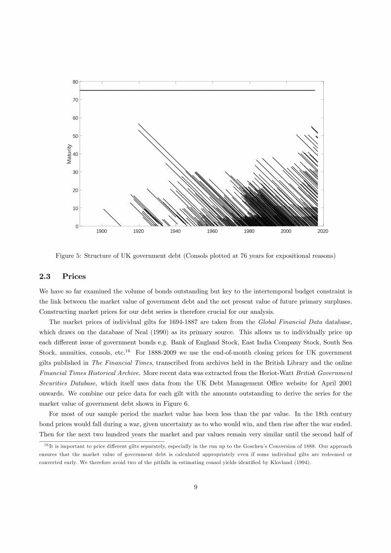
Figure 5 shows another feature of debt management. It plots the distribution by maturity of gilts out-
standing over time. If in any specific year a government has a bond with 8 years left to redemption then
that is indicated with a solid square at maturity 8. Similarly, if there is a government bond with 20 years
until its maturity date then a solid square is shown at 20. A solid row of solid squares from 1-20 would mean
the government has bonds outstanding at each maturity. Clear squares indicate no bond of that maturity is
outstanding. If governments do not buy back their debt each period then the maturity distribution shows a
natural persistence, i.e. a 10 year gilt in 2014 becomes a 9 year gilt in 2015 and a 8 year gilt in 2016 etc. As
shown by the presence of downward diagonals, government tends not to buyback debt until it matures at its
redemption date.14 ,15 Closer inspection shows that only 8 of the 537 gilts issued over this time period were
redeemed before their maturity date. In other words, once issued, governments tend not to repurchase gilts
until at or close to their redemption date. The other feature of Figure 5, related to Figure 3a, is how the
government has increasingly filled the maturity spectrum over time by seeking to fill “holes”, preferring to
issues gilts at each maturity.
14Faraglia et al (2017) document a similar finding for the US.15At the end of our sample the Bank of England as part of Quantitative Easing made large scale purchases of UK government
debt so that it now holds 25% of outstanding debt. Under a consolidated government budget constraint this entails the government
buying back before redemption. However our focus is on fiscal not monetary policy and as such we concentrate on the balance
sheet of the central government and do not include these as buybacks.
8
1900 1920 1940 1960 1980 2000 2020
Mat
urity
0
10
20
30
40
50
60
70
80
Figure 5: Structure of UK government debt (Consols plotted at 76 years for expositional reasons)
2.3 Prices
We have so far examined the volume of bonds outstanding but key to the intertemporal budget constraint is
the link between the market value of government debt and the net present value of future primary surpluses.
Constructing market prices for our debt series is therefore crucial for our analysis.
The market prices of individual gilts for 1694-1887 are taken from the Global Financial Data database,
which draws on the database of Neal (1990) as its primary source. This allows us to individually price up
each different issue of government bonds e.g. Bank of England Stock, East India Company Stock, South Sea
Stock, annuities, consols, etc.16 For 1888-2009 we use the end-of-month closing prices for UK government
gilts published in The Financial Times, transcribed from archives held in the British Library and the online
Financial Times Historical Archive. More recent data was extracted from the Heriot-Watt British Government
Securities Database, which itself uses data from the UK Debt Management Offi ce website for April 2001
onwards. We combine our price data for each gilt with the amounts outstanding to derive the series for the
market value of government debt shown in Figure 6.
For most of our sample period the market value has been less than the par value. In the 18th century
bond prices would fall during a war, given uncertainty as to who would win, and then rise after the war ended.
Then for the next two hundred years the market and par values remain very similar until the second half of
16 It is important to price different gilts separately, especially in the run up to the Goschen’s Conversion of 1888. Our approach
ensures that the market value of government debt is calculated appropriately even if some individual gilts are redeemed or
converted early. We therefore avoid two of the pitfalls in estimating consol yields identified by Klovland (1994).
9
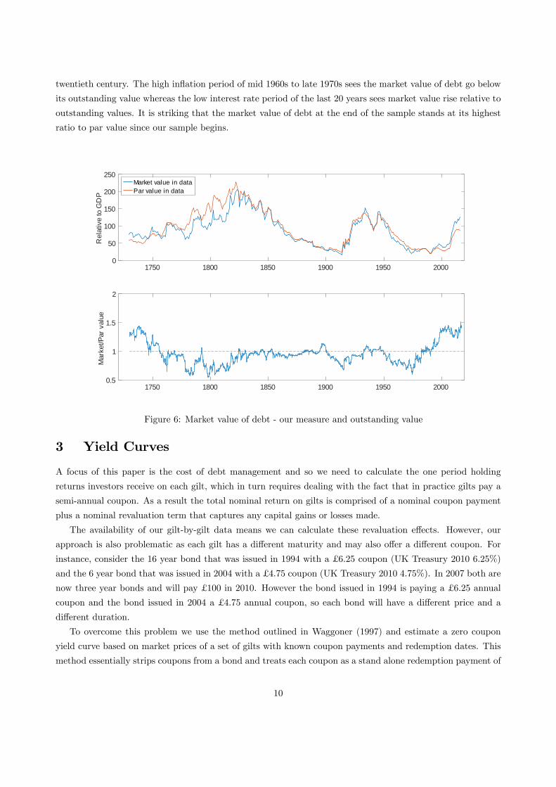
twentieth century. The high inflation period of mid 1960s to late 1970s sees the market value of debt go below
its outstanding value whereas the low interest rate period of the last 20 years sees market value rise relative to
outstanding values. It is striking that the market value of debt at the end of the sample stands at its highest
ratio to par value since our sample begins.
1750 1800 1850 1900 1950 2000
Rel
ativ
e to
GD
P
0
50
100
150
200
250Market value in dataPar value in data
1750 1800 1850 1900 1950 2000
Mar
ket/P
ar v
alue
0.5
1
1.5
2
Figure 6: Market value of debt - our measure and outstanding value
3 Yield Curves
A focus of this paper is the cost of debt management and so we need to calculate the one period holding
returns investors receive on each gilt, which in turn requires dealing with the fact that in practice gilts pay a
semi-annual coupon. As a result the total nominal return on gilts is comprised of a nominal coupon payment
plus a nominal revaluation term that captures any capital gains or losses made.
The availability of our gilt-by-gilt data means we can calculate these revaluation effects. However, our
approach is also problematic as each gilt has a different maturity and may also offer a different coupon. For
instance, consider the 16 year bond that was issued in 1994 with a £ 6.25 coupon (UK Treasury 2010 6.25%)
and the 6 year bond that was issued in 2004 with a £ 4.75 coupon (UK Treasury 2010 4.75%). In 2007 both are
now three year bonds and will pay £ 100 in 2010. However the bond issued in 1994 is paying a £ 6.25 annual
coupon and the bond issued in 2004 a £ 4.75 annual coupon, so each bond will have a different price and a
different duration.
To overcome this problem we use the method outlined in Waggoner (1997) and estimate a zero coupon
yield curve based on market prices of a set of gilts with known coupon payments and redemption dates. This
method essentially strips coupons from a bond and treats each coupon as a stand alone redemption payment of
10
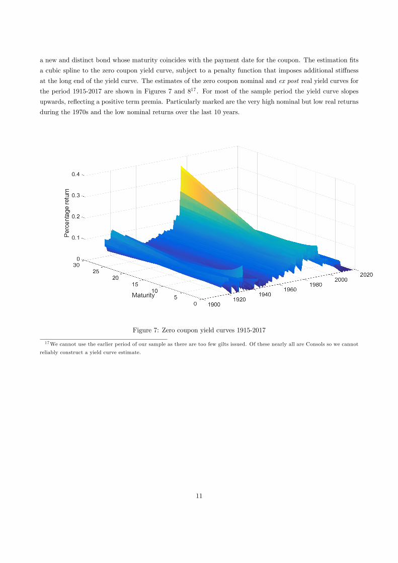
a new and distinct bond whose maturity coincides with the payment date for the coupon. The estimation fits
a cubic spline to the zero coupon yield curve, subject to a penalty function that imposes additional stiffness
at the long end of the yield curve. The estimates of the zero coupon nominal and ex post real yield curves for
the period 1915-2017 are shown in Figures 7 and 817 . For most of the sample period the yield curve slopes
upwards, reflecting a positive term premia. Particularly marked are the very high nominal but low real returns
during the 1970s and the low nominal returns over the last 10 years.
Figure 7: Zero coupon yield curves 1915-2017
17We cannot use the earlier period of our sample as there are too few gilts issued. Of these nearly all are Consols so we cannot
reliably construct a yield curve estimate.
11

1920 1940 1960 1980 2000 20200.2
0.1
0
0.1
0.2Yield on 1 year bond
NominalReal
1920 1940 1960 1980 2000 20200.2
0.1
0
0.1
0.2Yield on 3.5 year bond
NominalReal
1920 1940 1960 1980 2000 20200.2
0.1
0
0.1
0.2Yield on 10 year bond
NominalReal
1920 1940 1960 1980 2000 20200.04
0.02
0
0.02
0.04
0.06Term premium
Figure 8: Selected yields (term premium is difference between yields on 10 year and 3.5 year bonds)
Figure 9 plots the mean nominal and ex post real yield curves for each maturity as well as their standard
deviations. Nominal and real gilts both show a clear term premium, with the volatility of nominal yields, as
expected, increasing with maturity.
Maturity0 5 10 15 20 25 30M
ean
of n
omin
al y
ield
4.5
5
5.5
6
6.5
SD o
f nom
inal
yie
ld
10
12
14
16
18
Period0 5 10 15 20
Mea
n of
real
yie
ld
0.5
1
1.5
2
SD o
f rea
l yie
ld
5
10
15
20
Figure 9: Mean and volatility of yield by maturity for nominal and real yields
The average one year holding period return for the whole portfolio from 1730 to 2016 is 4.4% in nominal
terms and 2.6% in real terms. The return shows clear shifts between decades and is volatile - ranging from
a maximum of +20% to a minimum of -6%. Between 1890 and 1918 bond holders earned an average real
return of -1.1% and between 1946 and 1970 a real return of -1.9%. Conversely, between 1919 and 1939 they
12
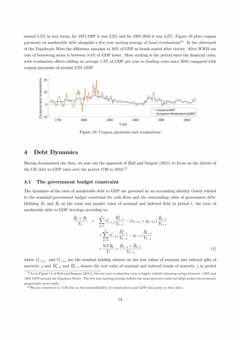
earned 5.5% in real terms, for 1971-1997 it was 2.2% and for 1997-2016 it was 4.2%. Figure 10 plots coupon
payments on marketable debt alongside a five year moving average of bond revaluations18 . In the aftermath
of the Napoleonic Wars the difference amounts to 10% of GDP as bonds soared after victory. After WWII our
cost of borrowing series is between 3-4% of GDP lower. Most striking is the period since the financial crisis,
with revaluation effects adding an average 1.3% of GDP per year to funding costs since 2010 compared with
coupon payments of around 2.3% GDP.
Y ear1750 1800 1850 1900 1950 2000
Cou
pons
and
reva
luat
ions
10
0
10
20
Coupons/GDP(Coupons+Revaluations)/GDP
Figure 10: Coupon payments and revaluations
4 Debt Dynamics
Having documented our data, we now use the approach of Hall and Sargent (2011) to focus on the drivers of
the UK debt to GDP ratio over the period 1730 to 2016.19
4.1 The government budget constraint
The dynamics of the ratio of marketable debt to GDP are governed by an accounting identity closely related
to the standard government budget constraint for cash flows and the outstanding value of government debt.
Defining B̃t and B̄t as the total real market value of nominal and indexed debt in period t, the ratio of
marketable debt to GDP develops according to:
B̃t + B̄tYt
=
n∑j=1
r̃jt−1,tB̃jt−1Yt−1
− (πt−1,t + gt−1,t)B̃t−1Yt−1
+
n∑j=1
r̄jt−1,tB̄jt−1Yt−1
− gt−1,tB̄t−1Yt−1
+NFRtYt
+B̃t−1 + B̄t−1
Yt−1(1)
where r̃jt−1,t and r̄jt−1,t are the nominal holding returns on the real values of nominal and indexed gilts of
maturity j and B̃jt−1 and B̄jt−1 denote the real value of nominal and indexed bonds of maturity j in period
18As in Figure 11 of Hall and Sargent (2011), the one year revaluation term is highly volatile (showing swings between +40% and
-20% GDP around the Napolean Wars). The five year moving average follows the same general trends but helps isolate the economic
magnitudes more easily.19We are restricted to 1730 due to the nonavailability of consol prices and GDP data prior to that date.
13

t− 1. Inflation πt−1,t is measured by the growth in the GDP deflator between periods t− 1 and t, and gt−1,tdenotes the growth in real GDP between periods t− 1 and t. The term NFRt is the net funding requirement,
the quantity of marketable debt the government issues in the period to finance its primary deficit in period t.
In the case where no nonmarketable debt is used NFRt is the primary deficit.
In other words, debt increases because of the upward pressure of nominal return paid to bond holders,
is reduced by inflation and GDP growth (which affect the growth adjusted real interest rate) and is pushed
upwards by the current primary deficit.
4.2 Decomposition
Table 1 shows our decomposition of debt dynamics for the period 1730 to 2016.20 Over the whole period
government debt rises from 75% to 126% of GDP, an increase of 51%. The only factor consistently leading
to upward pressure on debt is the nominal return. Over the entire sample bond holders received a return
significantly in excess of inflation and GDP growth - the nominal return averaging 4.4%, inflation 1.8% and
real growth 1.8%. Inflation and GDP growth all helped bring down the level of debt, as does the fact that the
government on average runs a primary surplus over the period 1730 to 2016.
There are however, not surprisingly, distinct differences across periods. Using major wars to pin down
subsamples (1763 the end of the Seven Year War, 1815 the end of the Napoleonic war, 1914 start of WWI,
1945 end of WWII) and then sub-dividing the modern period to capture changes in inflation and the financial
crisis, we find considerable variation. Between 1730 and 1763 the Seven Year War leads to an increase in
debt. During the 18th century bond investors demanded a high risk premium for war financing so the nominal
return contributes substantially to the debt increase. However, governments during this time ran a tight fiscal
policy and a series of primary surpluses restrained the debt. During the 18th century bond prices fell during
war times so there is a small but favourable revaluation effect which helps towards fiscal solvency. The period
1764-1815 includes the Napoleonic war and saw an increase in debt of 32%. The same pattern as for the Seven
Year war is noticeable - bond holders receive a high return which pushes debt higher, the government runs
a small average surplus to try and restrain debt, and there is a small favourable revaluation effect on bond
prices. The long and relatively peaceful period between 1816 and 1913 sees debt fall by more than 100% GDP.
Bond holders again receive a good return (an average real return of 3.8%, the highest across all subsamples but
equal to that in the final period) but the debt is reduced by a substantial contribution from primary surpluses.
The period 1914 to 1945 includes two major world wars and a decade-long economic slump in the 1920s, so
government debt increases by 122% of GDP. Nominal returns again contribute to an increase in debt, there
is an unfavourable revaluation effect from bond prices, and a large number of primary deficits lead to higher
debt.20Crafts (2016) performs a similar analysis for UK government debt from 1831 to 2015 but focuses on the face rather than the
market value of debt, so does not consider the revaluation effects that play an important role in our analysis.
14
StartDebttoGDP
EndDebttoGDP
ChangeinDebttoGDP
ContributionofNominalReturn
-ofwhichcoupons
-ofwhichrevaluations
ContributionofInflation
ContributionofGDPGrowth
ContributionofNewDebt
1730-2016 75.1 125.7 50.6 966.3 892.3 74.0 -253.8 -469.7 -192.3
1730-1815 75.1 134.3 59.2 275.7 299.0 -23.3 -73.3 -106.2 -37.0
1816-1913 134.3 17.2 -117.1 391.7 314.9 76.8 38.3 -209.4 -337.6
1914-2016 17.2 125.7 108.5 299.0 278.4 20.6 -218.7 -154.1 182.3.9
1730-1763 75.1 101.9 26.8 70.5 76.8 -6.2 -5.2 -24.7 -13.8
1764-1815 101.9 134.3 32.4 205.1 222.2 -17.1 -68.1 -81.4 -23.2
1816-1913 134.3 17.2 -117.1 391.7 314.9 76.8 38.3 -209.4 -337.6
1914-1945 17.2 139.1 121.9 135.8 114.8 21.0 -57.9 -58.8 102.8
1946-1970 139.1 28.6 -110.5 35.8 65.6 -29.9 -88.7 -50.4 -7.2
1971-1997 28.6 43.9 15.3 66.9 60.6 6.3 -59.2 -21.0 28.5
1998-2016 43.9 125.7 81.8 60.5 37.4 23.1 -13.0 -24.0 58.2
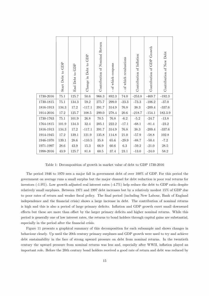
Table 1: Decomposition of growth in market value of debt to GDP 1730-2016
The period 1946 to 1970 sees a major fall in government debt of over 100% of GDP. For this period the
government on average runs a small surplus but the major channel for debt reduction is poor real returns for
investors (-1.9%). Low growth adjusted real interest rates (-4.7%) help reduce the debt to GDP ratio despite
relatively small surpluses. Between 1971 and 1997 debt increases but by a relatively modest 15% of GDP due
to poor rates of return and weaker fiscal policy. The final period (including New Labour, Bank of England
independence and the financial crisis) shows a large increase in debt. The contribution of nominal returns
is high and this is also a period of large primary deficits. Inflation and GDP growth exert small downward
effects but these are more than offset by the larger primary deficits and higher nominal returns. While this
period is generally one of low interest rates, the returns to bond holders through capital gains are substantial,
especially in the period after the financial crisis.
Figure 11 presents a graphical summary of this decomposition for each subsample and shows changes in
behaviour clearly. Up until the 20th century primary surpluses and GDP growth were used to try and achieve
debt sustainability in the face of strong upward pressure on debt from nominal returns. In the twentieth
century the upward pressure from nominal returns was less and, especially after WWII, inflation played an
important role. Before the 20th century bond holders received a good rate of return and debt was reduced by
15
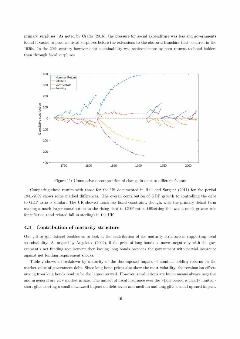
primary surpluses. As noted by Crafts (2016), the pressure for social expenditure was less and governments
found it easier to produce fiscal surpluses before the extensions to the electoral franchise that occurred in the
1920s. In the 20th century however debt sustainability was achieved more by poor returns to bond holders
than through fiscal surpluses.
1750 1800 1850 1900 1950 2000
Cum
ulat
ive
cont
ribut
ion
400
300
200
100
0
100
200
300
400Nominal ReturnInflationGDP GrowthFunding
Figure 11: Cumulative decomposition of change in debt to different factors
Comparing these results with those for the US documented in Hall and Sargent (2011) for the period
1941-2009 shows some marked differences. The overall contribution of GDP growth to controlling the debt
to GDP ratio is similar. The UK showed much less fiscal constraint, though, with the primary deficit term
making a much larger contribution to the rising debt to GDP ratio. Offsetting this was a much greater role
for inflation (and related fall in sterling) in the UK.
4.3 Contribution of maturity structure
Our gilt-by-gilt dataset enables us to look at the contribution of the maturity structure in supporting fiscal
sustainability. As argued by Angeletos (2002), if the price of long bonds co-moves negatively with the gov-
ernment’s net funding requirement then issuing long bonds provides the government with partial insurance
against net funding requirement shocks.
Table 2 shows a breakdown by maturity of the decomposed impact of nominal holding returns on the
market value of government debt. Since long bond prices also show the most volatility, the revaluation effects
arising from long bonds tend to be the largest as well. However, revaluations are by no means always negative
and in general are very modest in size. The impact of fiscal insurance over the whole period is clearly limited -
short gilts exerting a small downward impact on debt levels and medium and long gilts a small upward impact.
16

ContributionofReturnonNominalGilts
ContributionofReturnonIndex-linkedGilts
CouponsonShortGilts,j≤
7
CouponsonMediumGilts,
7<j≤
15
CouponsonLongGilts,j>
15
RevaluationsofShortGilts,j≤
7
RevaluationsofMediumGilts,
7<j≤
15
RevaluationsofLongGilts,j>
15
1730-2016 947.1 19.2 72.1 70.7 749.5 -1.3 13.1 62.2
1730-1815 275.7 0 0 0.0 298.9 0 0 -23.3
1816-1913 391.7 0 0.3 0.1 314.5 0.1 0.0 76.7
1914-2016 279.8 19.2 71.8 70.6 136.0 -1.4 13.1 8.9
1730-1763 70.5 0 0 0 76.8 0 0 -6.3
1764-1815 205.2 0 0 0 222.2 0 0 -17.1
1816-1913 391.7 0 0.3 0.1 314.5 0.1 0.0 76.7
1914-1945 135.8 0 21.5 29.4 63.8 -2.2 5.7 17.6
1946-1970 35.8 0 14.1 11.3 40.3 1.4 -1.3 -29.9
1971-1997 64.7 2.2 21.6 19.8 19.2 2.4 3.3 0.6
1998-2016 43.5 17.0 14.7 10.1 12.7 -2.9 5.4 20.6
Table 2: Role of debt structure in fiscal dynamics 1730-2016
Figure 12 shows one period holding returns broken down by maturity. Consistent with the theory, long
bond prices prove the most volatile and substantial negative returns after 1940 play a role in lowering the
debt to GDP ratio after WWII and again in the 1970s. However, there are also plenty of periods where the
covariance goes the other way and long bond prices rise when debt is increasing - the 1930s and the most
recent financial crisis being obvious examples.
17

1920 1930 1940 1950 1960 1970 1980 1990 2000 2010 2020
Ret
urn
10
5
0
5
10
15
short <=7 yearsmedium 715 yearslong > 15 years
Figure 12: One period returns across three maturities
To consider in greater detail the fiscal insurance provided by long bonds, consider Figure 13(a) which plots
the government’s annual primary deficit as a percentage of GDP against the corresponding annual percentage
revaluation of a 3% Treasury consol from 1730 (when the consol was first issued) to 2014 (when it was
redeemed). The points to the right of the scatter plot are all for the years of WWI and WWII when the
primary deficit was especially high. The correlation between the primary deficit and revaluations of the consol
across the whole sample period is very slightly positive and insignificant at 0.006 - the incorrect sign for fiscal
insurance.
Primary def ic it0.2 0 0.2 0.4 0.6
Rev
alua
tion
of C
onso
l
0.4
0.2
0
0.2
0.4
0.6(a) Primary deficit vs Revaluation
Y ears0 2 4 6 8 10
Rev
alua
tion
of C
onso
l
0.03
0.02
0.01
0
0.01
0.02(b) Response to a primary deficit shock
Figure 13: Primary deficit and revaluation of 3% Treasury Consol.
The correlations between the primary deficit and revaluations of the consol strengthen if we consider
correlations at leads and lags, which suggests that a simple bivariate vector autoregression analysis may be
useful. Figure 13(b) presents the resulting impulse response function, showing how the consol is revalued
after a one percentage point shock to the primary deficit as a percentage of GDP. Identification is achieved
by assuming that shocks to the price of consols have no contemporaneous effects on the primary deficit, the
lag length of the vector autoregression is 4 and 95% confidence intervals are shown. It is diffi cult to identify
shocks by contemporaneous zero restrictions with annual data, so our results should be treated with caution
but the tentative conclusion from Figure 13(b) is that long bonds are unlikely to provide the government with
significant fiscal insurance. Bond prices move in the right direction after a primary deficit shock, but the
movement is transitory and only borderline significant.
18
4.4 Wars
Our long data sample enables us to examine how several different wars were financed. A cursory glance
at British history over this period reveals a near never-ending list of conflicts (in only 52 years from 1700
to 2017 is the UK not involved in some form of military conflict). However, examination of the government
expenditure series suggests the following as substantial conflicts in terms of their financing needs: 1740-49 (War
of Austrian Succession including King George’s War and War of Jenkins’Ear), 1756-1764 (Seven Years’War),
1775-1786 (War of American Independence, Anglo-French War, Anglo-Spanish War, Anglo-Dutch War), 1793-
1815 (including War of French Revolution and Napoleonic Wars), 1914-1919 (WWI) and 1939-46 (WWII).21
Table 3 shows the decomposition of debt dynamics for these periods and compares it to periods of peace.
All these wars lead to a broadly similar increase in debt of around 30% of GDP during the time of conflict,
although in many cases debt continues to increase after the conflict has ceased. Comparing times of war and
times of peace, the obvious differences are i) during war the country runs deficits and in peace surpluses ii)
during wars inflation plays twice as large a role in containing debt iii) on average bond prices provide some
fiscal insurance by falling during war and rising in peace iv) the contribution of GDP growth to lowering the
debt to GDP ratio is about twice as important during wars v) long bonds are responsible for all of the fiscal
insurance effect but their most important role is as a conduit for the inflation effect which is around four times
larger than the revaluation effect. The nominal return on government bonds decreases in periods of war (3.7%
compared to 4.7% during peace), as does the real return (0.7% compared to 3.1%), due to a rise in inflation
(3.0% compared to 1.6%).
Whilst there is considerable similarity across the different wars there are also inevitable differences. The
role of inflation in financing wars has become more significant over time and the revaluation/fiscal insurance
effect is particularly unstable across different time periods. In general, wars are financed by deficits that are
subsequently offset by surpluses in peacetime when long bond holders in particular experience a low real return
due to higher inflation.
21These dates are based on high levels of government expenditure and so tend to last a year or two longer than conventional
dates of the conflicts because of demobilisation costs.
19

StartDebttoGDP
EndDebttoGDP
ChangeinDebttoGDP
ContributionofNominalReturn
-ofwhichcoupons
-ofwhichrevaluations
ContributionofInflation
ContributionofGDPGrowth
ContributionofNewDebt
Wars
1740-1749 70.1 97.3 27.2 24.0 21.8 2.2 -4.3 -4.4 12.0
1756-1764 74.5 103.4 28.9 22.8 22.8 0.1 -10.3 -7.3 23.6
1775-1786 90.5 116.4 25.9 36.7 40.8 -4.1 -10.1 -13.0 12.3
1793-1815 100.7 134.3 33.6 95.1 118.4 -23.2 -44.2 -48.3 30.9
1914-1919 17.2 52.8 35.6 3.7 8.7 -5.0 -34.2 0.9 65.2
1939-1945 115.2 141.5 26.4 39.0 25.0 14.1 -47.7 -14.5 49.5
Peace
1730-1739 75.1 70.1 -5.0 23.4 22.3 1.1 7.9 -8.2 -28.1
1750-1755 97.3 74.5 -22.9 5.9 13.5 -7.6 0.6 -4.8 -24.6
1765-1774 103.4 90.5 -12.9 34.1 32.4 1.7 -7.8 -4.3 -34.9
1787-1792 116.4 100.7 -15.7 33.5 27.1 6.4 -5.1 -15.8 -28.3
1816-1913 134.3 17.2 -117.1 391.7 314.9 76.8 38.3 -209.4 -337.6
1920-1938 52.8 115.2 62.4 102.8 84.8 17.9 19.9 -41.8 -18.5
1947-2016 141.6 125.7 -15.9 153.6 159.9 -6.4 -156.7 -98.7 86.0
Table 3: Debt dynamics in war and peace
4.5 Financial Crises
The surge in government debt since the 2007-9 financial crises raises the issue of how the UK has responded
to financial crises over our 323 year sample. We follow Capie (2014) in selecting 1825 (run on country banks),
1837 (US crisis and UK balance of payments crisis), 1847 (Bill market crisis), 1857 (US panic, Borough Bank
of Liverpool), 1866 (Overend Gurney) and 2007-2009 (Global Financial Crisis) as financial crises. There are
many other notable periods of financial instability (e.g., Barings in 1890, the accepting house crises in 1914 and
the secondary banking crisis between 1973-75) but based on the Schwarz (1986) definition of a financial crises
as one which actively threatens the payments system these are the major financial crises. It is striking how few
financial crises there are over the period using this stricter definition. The 18th century sees none (according
to Capie (2014) the credit system is still undeveloped as evidenced by a low money multiplier so deposits and
reserves are close in value) and then between 1866 and 2006 there are no major system threatening crises.
20
Table 4 shows the debt dynamics for financial crisis periods (where we include three years after the financial
crisis) and contrasts them with periods of non-crises. Comparing averages we see i) crisis years witness an
increase in government debt whereas non-crisis years witness small declines in debt ii) on average financial
crises see fiscal policy reducing the value of debt not increasing it (the 2007-9 period being the major exception)
i.e. historically the government has tightened fiscal policy during financial crises to improve the fiscal position
iii) nominal holding returns tend to boost government debt more in crises than otherwise with most of that
contribution coming from an unfavourable revaluation of long bonds iv) low inflation during financial crises
tends to lead to a higher debt to GDP ratio.
The most striking difference between financial crises and other periods is the ex post real return on nominal
debt. During periods of financial crises the return is 4.9% compared with 0.2% otherwise. This is only partly
due to a fall in inflation (-0.5% compared to 0.2%), with the rest being due to upwards revaluation in bond
prices. Financial crises tend to be followed by low interest rates and bond price increases. Note that the most
recent 2007-9 financial crisis saw a real return of 4.7%, slightly above the average across the sample. This
upward shift in bond prices is important as it means that long bonds provide the opposite of fiscal insurance
during a financial crisis. One striking manifestation of this is the fact that, at the end of our sample period
after the 2007-9 financial crisis, the market value of government debt is at its highest premium relative to its
face value for the whole 323 years of our sample.
21

StartDebttoGDP
EndDebttoGDP
ChangeinDebttoGDP
ContributionofNominalReturn
-ofwhichcoupons
-ofwhichrevaluations
ContributionofInflation
ContributionofGDPGrowth
ContributionofNewDebt
Financial crises
1825-1828 201.9 182.0 -19.9 13.9 24.8 -10.9 -0.6 -10.6 -22.7
1837-1842 148.6 171.3 22.6 38.8 30.1 8.7 14.0 -4.9 -25.2
1847-1850 135.4 153.8 18.4 25.1 17.5 7.5 12.3 -1.8 -17.2
1857-1860 104.0 99.9 -4.1 11.9 13.4 -1.5 2.0 -7.4 -10.6
1866-1869 73.0 71.6 -1.4 14.0 9.6 4.4 1.6 -6.0 -11.1
2007-2012 45.6 114.0 68.4 24.6 12.7 11.9 -4.4 -2.5 50.7
Normal times
1730-1824 75.1 201.9 126.8 415.0 363.3 51.7 -41.9 -135.4 -110.8
1829-1836 182.0 148.6 -33.3 52.1 46.5 5.6 6.1 -39.5 -52.0
1843-1846 171.2 135.4 -35.9 13.3 17.5 -4.2 -0.1 -33.3 -15.8
1851-1856 153.8 104.0 -49.8 17.6 21.7 -4.1 -20.8 -25.5 -21.2
1861-1865 99.9 73.0 -26.9 10.3 14.2 -3.8 -9.1 -10.5 -17.6
1870-2006 71.6 45.6 -26.0 309.6 310.8 -1.2 -208.7 -182.2 55.3
Table 4: Debt dynamics in financial crises and normal times
5 Assessing Debt Management Policy
The fact that our dataset is built up gilt-by-gilt means we can investigate what would have happened to UK
government debt under alternative issuance policies. In other words, we can use our estimates of the yield
curves and vary the maturity structure of government debt and see in an ex post sense which debt management
strategy would have performed best.
In performing these counterfactuals we follow Hall and Sargent (2010) in making a strong exogeneity
assumption that yields do not vary with the volume and maturity structure of government debt, i.e., that
the yield curve is unaffected by debt issuance. There are two reasons why varying the debt structure would
in practice influence yields. The first is at the heart of macroeconomic analyses of debt management, e.g.,
Aiyagari et al. (2002), Angeletos (2002), Buera and Nicolini (2004). In these models different issuance policies
lead to different market values of debt, and so different processes for tax rates and outcomes for consumption
and rates of return. The second channel is based on market microstructure. Debt management offi ces are very
22

concerned that if they try and sell too much of any particular maturity they will face liquidity effects which
adversely affect the price at which they can sell (see Guibaud, Nosbusch and Vayanos (2013)). The magnitude
of these effects differs across different maturities and is not linear (see Lou, Yan and Zhang (2013), Breedon
and Turner (2016) and Song and Zhu (2016)), implying that changing the composition of debt issuance will
affect yields.
Ignoring these two channels is clearly a limitation of our ex post counterfactuals. However, it is worth noting
that studies using structural models tend to find that variations in the maturity structure usually have very
limited macroeconomics spillovers. The results of Angeletos (2002), Buera and Nicolini (2004) and Faraglia et
al (2010) show that very large variations in the structure of debt bring about only small variations in macro
outcomes. The yield curve is generally quite flat, intertemporal effects are relatively small, and so large shifts
in how the government finances a given level of debt have little effect on economic outcomes. In terms of
liquidity effects, a later section addresses the robustness of our findings to their inclusion by investigating the
magnitude of effects required to offset any gains discovered by our counterfactuals.
5.1 Alternative Fiscal Histories
Table 1 showed how the total market value of UK national debt evolved over our sample period under observed
debt management. In this section we consider how that evolution would have differed if the government had
followed alternative debt management policies. We build multiple counterfactual scenarios that are differen-
tiated by the maturity of debt the government issues. The simplest counterfactuals assume the government
concentrates all its issuance in zero coupon nominal bonds of a specific maturity, i.e., the government only
ever issues bonds of 3, 5 or 10 year maturity. Subsequent counterfactuals permit a wider range of maturity
options as well as issuing a mix of bonds of different maturities.
When we change the maturity of debt we change the cash flow of government financing, as this depends
on both the current primary deficit and the value of bonds maturing each period. The first step in our
counterfactual is therefore to isolate the historical component of the primary deficit that was financed by the
issuance of marketable bonds?
(NFRt) and then construct alternative financing histories by using this and
recalculating the redemption profile of debt in light of the different issuance policy. We do this in the following
manner. At the beginning of our sample period all the national debt was in the form of consols so there are no
initial coupon or redemption payments on previously issued fixed term nominal debt. The government hence
issues Njt =?
NFRt/Pjt zero coupon bonds of maturity j for the first time at time t, where P
jt is the price of a
zero coupon bond of maturity j at time t. Issuing these bonds changes future redemptions, in particular the
government will have to fund?
NFRt+j+ Njt in j years’time, which will require issuing (?
NFRt+j +Njt)/Pjt+j
bonds. Moving forward recursively we can then construct counterfactual series for issuance, redemptions and
the market value of debt, under the exogeneity assumption that yields are unaffected by issuance.
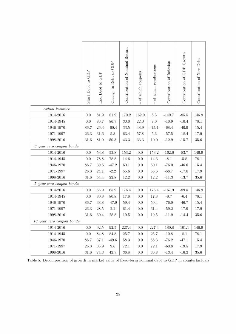
Table 5 presents results for the alternative debt management scenarios and shows that the level of debt
in 2016 would have been lower by 28.1% of GDP (a debt to GDP ratio of 53.8% rather than 81.9%) had
the government only issued 3 year bonds between 1914-2016. The corresponding debt to GDP ratio if the
government only issued 5 year bonds in this period would have been 65.9%, and for 10 year bonds 92.5%. As
the yield curve usually slopes upwards, issuance policies that concentrate on long maturities lead to higher
one period holding returns and hence higher levels of debt than policies based on short maturities.
23

Table 5 reports results from different sub-periods and Figure 14 shows graphically for every combination of
dates in our sample the periods over which 3, 5 or 10 year issuance would have performed best. In Table 5, only
for 1946-1970 do our alternative debt issuance policies produce worse end-of-period outcomes than the actual
UK debt management policy. This is also the period where long bonds perform best as it conforms closest
to the general insight of the optimal fiscal policy/debt management literature. Post war there is an increase
in government expenditure, the price of long bonds falls more than the price of short bonds, so an issuance
strategy based on long bonds helps insure the government against greater increases in taxation. However, in
the vast majority of subperiods this does not hold. Particularly striking is the most recent subperiod 1997-2016,
which suggests that the UK policy of focusing on issuing long maturity bonds led to a substantial increase
in the market value of debt. Long-term interest rates fell after the financial crisis, triggering unfavourable
revaluation effects and high one period holding returns on long bonds. This would have been avoided had the
government issued shorter maturity bonds.
Part of the reason why the policy of always issuing 3 year bonds performs so well is that the yield curve
usually slopes upwards, in which case short maturity bonds have a lower yield. However, the superior perfor-
mance when issuing 3 year bonds is due to more than just cheapness of the yield. Issuing only 3 year bonds also
outperforms an alternative policy in which the government issues 3, 5 or 10 year bonds each year depending
on which maturity has the lowest yield. Over the whole sample period 1914-2016, the cheapest yield policy
produces a final debt level of 72.2% of GDP, compared with 53.8% under the 3 year bond policy. Only for the
period 1946 to 1970 does the cheapest yield policy slightly outperform issuing 3 year bonds, because during
these years the 10 year yield is more often cheaper. The success of the 3 year bond policy is therefore not
purely due to the upward sloping nature of the yield curve.
24
StartDebttoGDP
EndDebttoGDP
ChangeinDebttoGDP
ContributionofNominalReturn
-ofwhichcoupons
-ofwhichrevaluations
ContributionofInflation
ContributionofGDPGrowth
ContributionofNewDebt
Actual issuance
1914-2016 0.0 81.9 81.9 170.2 162.0 8.3 -149.7 -85.5 146.9
1914-1945 0.0 86.7 86.7 30.0 22.0 8.0 -10.9 -10.4 78.1
1946-1970 86.7 26.3 -60.4 33.5 48.9 -15.4 -68.4 -40.9 15.4
1971-1997 26.3 31.6 5.3 63.4 57.8 5.6 -57.5 -18.4 17.9
1998-2016 31.6 81.9 50.3 43.3 33.3 10.0 -12.9 -15.7 35.6
3 year zero coupon bonds
1914-2016 0.0 53.8 53.8 153.2 0.0 153.2 -162.6 -83.7 146.9
1914-1945 0.0 78.8 78.8 14.6 0.0 14.6 -8.1 -5.8 78.1
1946-1970 86.7 39.5 -47.2 60.1 0.0 60.1 -76.0 -46.6 15.4
1971-1997 26.3 24.1 -2.2 55.6 0.0 55.6 -58.7 -17.0 17.9
1998-2016 31.6 54.4 22.8 12.2 0.0 12.2 -11.3 -13.7 35.6
5 year zero coupon bonds
1914-2016 0.0 65.9 65.9 176.4 0.0 176.4 -167.9 -89.5 146.9
1914-1945 0.0 80.8 80.8 17.8 0.0 17.8 -8.7 -6.4 78.1
1946-1970 86.7 38.8 -47.9 59.4 0.0 59.4 -76.0 -46.7 15.4
1971-1997 26.3 28.5 2.2 61.4 0.0 61.4 -59.2 -17.9 17.9
1998-2016 31.6 60.4 28.8 19.5 0.0 19.5 -11.9 -14.4 35.6
10 year zero coupon bonds
1914-2016 0.0 92.5 92.5 227.4 0.0 227.4 -180.8 -101.1 146.9
1914-1945 0.0 84.8 84.8 25.7 0.0 25.7 -10.8 -8.1 78.1
1946-1970 86.7 37.1 -49.6 58.3 0.0 58.3 -76.2 -47.1 15.4
1971-1997 26.3 35.9 9.6 72.1 0.0 72.1 -60.8 -19.5 17.9
1998-2016 31.6 74.3 42.7 36.8 0.0 36.8 -13.4 -16.2 35.6
Table 5: Decomposition of growth in market value of fixed-term nominal debt to GDP in counterfactuals
25

Start year1920 1940 1960 1980 2000 2020
End
yea
r
1910
1920
1930
1940
1950
1960
1970
1980
1990
2000
2010
2020
3 year bonds best5 year bonds best10 year bonds best
Figure 14: Comparison of counterfactuals with 3, 5 and 10 year bonds
6 Debt Management Considerations
Our counterfactual debt management experiments suggest that the UK government would for most periods
have been better off had it issued solely 3 year debt over the course of the twentieth century. However, our
counterfactuals were clearly very simple minded and based around issuing only one type of bond in large
volumes. Issuing large amounts of one specific bond raises a number of potential risks for a Debt Management
Offi ce. One such concern is around liquidity and the worry that concentrating issuance in large volumes will
drive prices against the government. Another concern is rollover risk, whereby if borrowing is concentrated
in single maturities then large deficits create a lumpy redemption profile. This leads to worries that the
government either will not be able to sell enough bonds to finance its activities or will find itself issuing large
amounts of bonds at a time when interest rates are very high. Issuing across a range of maturities helps to
lessen both these liquidity concerns and rollover risk. In addition to these practical debt management concerns,
the theoretical optimal debt management literature emphasises that the government may need to leverage its
position in order to get maximal benefits from long bonds and fully exploit movements in the yield curve. This
literature also normally assumes that each period the government buys back the entire stock of bonds (not
just those which are maturing) and then reissues, in doing so maximises the benefits of long bonds. As we
have so far excluded leverage as a debt management option and assumed no buyback, our findings favouring
short bonds may therefore be misleading. In this section we examine the robustness of our counterfactuals to
these features.
26

6.1 Liquidity Effects
In this section we calculate how large adverse liquidity effects would need to be to offset the gains displayed
in our counterfactual policies. The value of nominal debt to GDP in the data for 2016 is 81.9% whereas in the
counterfactual when the government only issues 3 year bonds it is 53.8%. How much would the yield curve
need to move in order to nullify this implied gain of 28.1% of GDP?
The yield to maturity ytmjt of a j period bond in period t satisfies
ytmjt =
(100
P jt
) 1j/12
− 1
where P jt is the current market of a nominal bond of face value £ 100 that matures in j periods. The counter-
factuals performed previously assume the government always received P jt for each £ 100 it promised to pay in j
periods, irrespective of the volume of debt it issued. We now allow for issuance to affect the cost of borrowing
through a premium x on the yield - the larger x the greater the impact of issuance on borrowing costs. In this
case the government receives only P̃ jt for each £ 100 it promises to pay in j periods, where
P̃ jt = 100
[(100
P jt
) 1j/12
+ x
]−j/12
Since P̃ jt < P jt the government needs to issue more debt to fulfil a given net funding requirement.
Premium on ytm (x in yield bp)0 20 40 60 80 100
Deb
tGD
P 20
16
50
100
150
200Data3 year5 year10 year
Figure 15: Effect of liquidity effects on counterfactual end of 2016 debt to GDP ratio
Figure 15 shows how the debt to GDP at the end of 2016 in our counterfactuals increases as the government
faces a higher premium on the yield to maturity. The critical break even value of x for the 3 year counterfactual
is 85 basis points and for the 5 year case 42 basis points. The 10 year counterfactual performs worse than the
actual UK debt management even without liquidity effects and so adding them only worsens things further.
Over the period 1914-2016 the average one period holding return on 3 year bonds is 5.3% so a liquidity
premium of 85 basis points is substantial. However so too is the increase in issuance required by our policy of
focusing just on three year bonds. For the same period the average annual issuance of debt with maturity of
3 ± 1 years (to allow for debt that was not issued with a maturity of exactly 3 years) amounted to 0.8% of
GDP whereas in our counterfactual with only 3 year bonds being issued the level of average annual issuance
rises to 15.2% of GDP. Therefore in order for three year bonds to outperform actual UK policy for the period
we require that the elasticity of the yield curve with respect to issuance is less than ∆Q/Q × ytm/∆ytm =
((15.2 − 0.8))/0.8 × 530/85 = 108. In practical terms, this means a doubling of issuance should lead to an
27

increase in yields of no more than 530/108 = 4.9 basis points. Breedon and Turner (2016) evaluate the costs
of the UK government both buying and issuing large quantities of government bonds. They report in their
Table A2.1 that a doubling in the value of issuance moves yields by a maximum of 3.300× log(2) = 2.3 basis
points, depending on the precise specification estimated. This is lower than the critical value calculated above
suggesting that the 3 year bond counterfactual will continue to generate gains even allowing for liquidity effects.
6.2 Refinancing Risk
The current objective of the UK Debt Management Offi ce is to “minimise, over the long term, the costs of
meeting the government’s financing needs, taking into account risk...”Issuing short bonds requires constantly
rolling over large volumes of debt each period, exposing the debt management offi ce to both interest rate risk
(defined by the Debt Management Offi ce as “interest rate exposure arising when new debt is issued”) and
refinancing risk (“interest rate exposure arising when debt is rolled over, with an increase in refinancing risk
if redemptions are concentrated in particular years”). This section extends our counterfactuals to take these
risks into account.
We quantify the risks and vulnerabilities in our counterfactuals by recognising that there are likely to be
implementation lags in policy. If the government has to commit to a fixed volume of bond issuance at least one
period in advance then they will face interest rate risk (the market price may fall short of what is expected)
and refinancing risk (different maturity profiles will lead to different gross funding requirements). Inspired by
the finance literature on Value at Risk, our preferred risk measure is the prospective shortfall in bond issuance
receipts that the government suffers when bond price movements are in their 5th most unfavourable percentile.
For example, a 1.5% level for the 5% Value of Risk measure means there is a 5% probability that a government
deciding issuance in advance will face a shortfall in receipts of at least 1.5% of GDP. Two countervailing forces
will be at work when comparing the Value at Risk across different maturities. Firstly, long bonds will typically
be bad for Value at Risk because they concentrate issuance at the long end of the yield curve where prices
are volatile. Secondly, long bond policies tend to be good for Value at Risk as they reduce gross issuance and
debt rollover each period.
28

Av erage debtGDP30 40 50 60
Ave
rage
VaR
1
1.5
2
2.5
3
1
2
3 4567
89
10
111213
14
15
16
17
18
19
20
(a) One maturity strategy
Av erage debtGDP30 40 50 60
Ave
rage
VaR
1
1.5
2
2.5
3(b) Two maturity strategy
Figure 16: Combinations of average VaR and debt-to-GDP ratio with different issuance strategies
Figure 16a shows combinations of average Value at Risk and average debt (both expressed as a percentage
of GDP) that are achieved over the period 1914-2016 by the simplest counterfactual scenarios in which the
government always issues zero coupon nominal bonds of a given maturity one period in advance. Policies based
on issuing bonds of an integer number of years to maturity are shown by large dots and labelled 1, 2, 3 and
so on. Smaller dots are for policies that issue non-integer maturities such as 2.5 years.
Figure 16a shows a clear U-shape, with Value at Risk first falling and then rising as maturity increases.22
To the right of the bottom of the U-shape, increasing the maturity of issuance allows the government to roll
over a smaller proportion of debt each period, but issuing longer bonds is expensive and risky in itself so
the government ends up with both a higher debt stock and a greater absolute need to roll over debt each
period. Figure 16b shows the average Value at Risk and average debt outcomes for counterfactuals in which
the government can issue fixed proportions of two zero coupon nominal bonds of different maturity each period.
We are interested in the most effi cient maturity structures that minimise the Value at Risk for a given debt
level, so Figure 17 plots the convex hulls of Figure 16 alongside the convex hull associated with an issuance
policy based around three distinct bonds. It is noticeable that the latter provides relatively small gains so we
focus below on the two bond case.22The pattern is robust to assuming an implementation lag of more than one period in the Value at Risk calculation. Longer
implementation lags lead to higher Values at Risk but still produce a U-shape.
29
Average debtGDP25 30 35 40 45 50 55 60 65
Aver
age
VaR
1.2
1.3
1.4
1.5
1.6
1.7
1.8
1.9
2
Data
One maturity strategyTwo maturity strategyThree maturity strategy
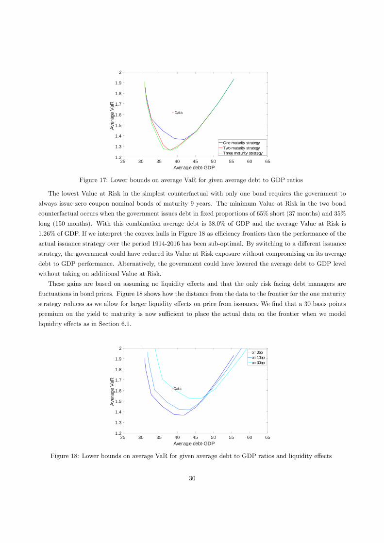
Figure 17: Lower bounds on average VaR for given average debt to GDP ratios
The lowest Value at Risk in the simplest counterfactual with only one bond requires the government to
always issue zero coupon nominal bonds of maturity 9 years. The minimum Value at Risk in the two bond
counterfactual occurs when the government issues debt in fixed proportions of 65% short (37 months) and 35%
long (150 months). With this combination average debt is 38.0% of GDP and the average Value at Risk is
1.26% of GDP. If we interpret the convex hulls in Figure 18 as effi ciency frontiers then the performance of the
actual issuance strategy over the period 1914-2016 has been sub-optimal. By switching to a different issuance
strategy, the government could have reduced its Value at Risk exposure without compromising on its average
debt to GDP performance. Alternatively, the government could have lowered the average debt to GDP level
without taking on additional Value at Risk.
These gains are based on assuming no liquidity effects and that the only risk facing debt managers are
fluctuations in bond prices. Figure 18 shows how the distance from the data to the frontier for the one maturity
strategy reduces as we allow for larger liquidity effects on price from issuance. We find that a 30 basis points
premium on the yield to maturity is now suffi cient to place the actual data on the frontier when we model
liquidity effects as in Section 6.1.
Average debtGDP25 30 35 40 45 50 55 60 65
Aver
age
VaR
1.2
1.3
1.4
1.5
1.6
1.7
1.8
1.9
2
Data
x=0bpx=10bpx=30bp
Figure 18: Lower bounds on average VaR for given average debt to GDP ratios and liquidity effects
30

To consider the impact of other risks take the case of a buyers strike, e.g., where not all bonds can
be sold. In Figure 17 the distance between the data and the 9 year counterfactual is a Value at Risk of
1.62% − 1.37% = 0.25% of GDP. Consider the arbitrary risk of a buyers strike in which market participants
were only prepared to purchase 90% of the bonds the government issued. The average annual issuance of 9
year bonds under our counterfactual is 4.9% of GDP so if the probability of the new strategy inducing a 10%
buyers strike were 5% then we would need to add 0.49% of GDP to our Value at Risk measure. So long as the
probability of a buyers strike is less than 5% × 0.25/0.49 = 2.4% then there would be no rise in total Value
at Risk. In other words, as long as implementation fails less than once in 40 years then the additional risk is
tolerable and does not substantially affect our conclusion.
6.3 Leverage
The superior outcome of our counterfactual 3 year funding strategy raises the issue of whether even better
performance were possible if the government took a leveraged position. Alternatively, leveraging could un-
dermine the superior performance of borrowing using short maturities. As emphasised by Buera and Nicolini
(2004) the usual optimal debt management literature recommendation of issuing long bonds involves highly
leveraged positions in order to magnify the limited shifts in the yield curve that occur in practice.
To investigate the effects of leverage we return to the counterfactuals in which the government issues
two bonds of different maturities (but in fixed proportions). We model leverage strategies by allowing the
government to issue a negative quantity of one of the bonds, i.e. the proportions of each bond are −z and 1+z
respectively, where z > 0. The results are shown in Figure 19, which reproduces the red effi ciency frontier
from Figure 17 as the baseline case with no over-issuance or leverage.
Average debtGDP25 30 35 40 45 50 55 60 65
Ave
rage
VaR
1.2
1.4
1.6
1.8
2
2.2
2.4
Data
Baseline issuance10% overissuance20% overissuance30% overissuance
Figure 19: Lower bounds on average VaR and average debt to GDP ratios with leverage
Over-issuance facilitates two types of outcome that were previously unattainable. In the south east of
Figure 19 the government can lower its Value at Risk exposure without increasing the average debt to GDP
ratio. These outcomes are achieved by the government over-issuing long bonds, although the benefits here
are somewhat illusory since all these new outcomes are dominated by ones attainable without leverage. Of
greater interest are the new possibilities in the north west of Figure 19, which arise when the government
31

over-issues short debt. By adopting this strategy the government is able to reduce average debt to GDP
levels below anything possible with non-leveraged strategies. Because short rates are less than long rates the
government can reduce debt by overborrowing short and investing in other assets. The drawback is that these
new outcomes are all associated with very high Value at Risk, as over-issuance exposes the government to
risk on both its borrowing and on its savings. Therefore at least within this Value at Risk framework using
leverage neither changes our conclusions about the attractiveness of long bonds nor suggests an alternative
best practice debt portfolio from our counterfactual analysis. Obviously leverage involves the government
taking even larger positions than in our standard counterfactuals. If liquidity effects and transaction costs are
important then this makes using leverage even less attractive.
6.4 Buyback
We have so far followed observed practice and assumed that once the government issues a bond it does not
repurchase it before maturity. As shown in Faraglia et al (2017), under incomplete markets the assumption
as to whether the government does or does not buy back its own debt before maturity matters as it affects
the timing of cash flows, reduces the effectiveness of long bonds in providing fiscal insurance and creates a
“lumpiness” in the repayments profile. We therefore introduce the possibility of government buybacks one
year after issuance to see if this lessens the desirability of using short bonds.
Table 6 reports the counterfactual evolution of nominal debt to GDP when the government buys back each
bond 12 months after it has been issued. In comparison with our previous results of Table 5, there are only
a few cases in which the buyback strategy outperforms no buyback. The most notable of these is the period
1946-1970 where buyback strategies dominate irrespective of whether the government issues 3, 5 or 10 year
bonds. Not surprisingly this is also the period where we found that long bond issuance dominated 3 year
issuance under no buyback. During this period the behaviour of long bond prices offers fiscal insurance, and
performing buyback increases the ability of long bonds to provide that fiscal insurance.
Note however that even under buyback the relative performance of 3, 5 and 10 year bonds strategies
remains as before. Issuing and buying back 10 year bonds is particularly undesirable in the most recent period
1998-2016, once more underlining the expensive nature of long bonds after a financial crisis.
32
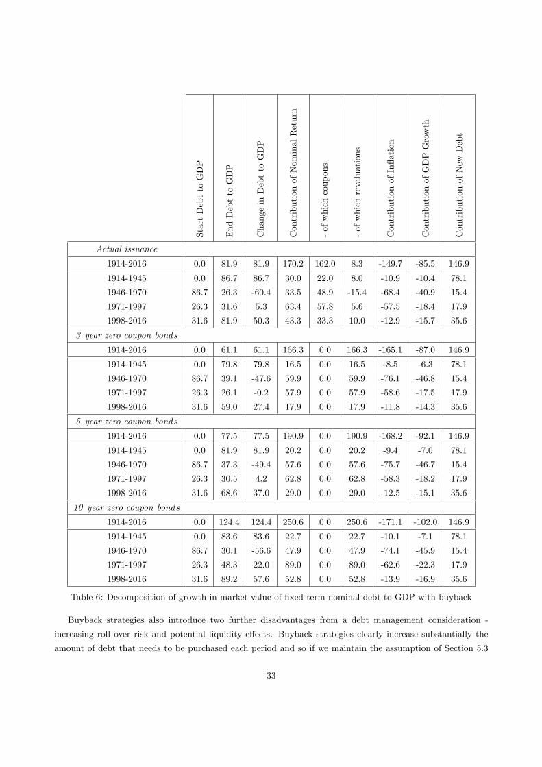
StartDebttoGDP
EndDebttoGDP
ChangeinDebttoGDP
ContributionofNominalReturn
-ofwhichcoupons
-ofwhichrevaluations
ContributionofInflation
ContributionofGDPGrowth
ContributionofNewDebt
Actual issuance
1914-2016 0.0 81.9 81.9 170.2 162.0 8.3 -149.7 -85.5 146.9
1914-1945 0.0 86.7 86.7 30.0 22.0 8.0 -10.9 -10.4 78.1
1946-1970 86.7 26.3 -60.4 33.5 48.9 -15.4 -68.4 -40.9 15.4
1971-1997 26.3 31.6 5.3 63.4 57.8 5.6 -57.5 -18.4 17.9
1998-2016 31.6 81.9 50.3 43.3 33.3 10.0 -12.9 -15.7 35.6
3 year zero coupon bonds
1914-2016 0.0 61.1 61.1 166.3 0.0 166.3 -165.1 -87.0 146.9
1914-1945 0.0 79.8 79.8 16.5 0.0 16.5 -8.5 -6.3 78.1
1946-1970 86.7 39.1 -47.6 59.9 0.0 59.9 -76.1 -46.8 15.4
1971-1997 26.3 26.1 -0.2 57.9 0.0 57.9 -58.6 -17.5 17.9
1998-2016 31.6 59.0 27.4 17.9 0.0 17.9 -11.8 -14.3 35.6
5 year zero coupon bonds
1914-2016 0.0 77.5 77.5 190.9 0.0 190.9 -168.2 -92.1 146.9
1914-1945 0.0 81.9 81.9 20.2 0.0 20.2 -9.4 -7.0 78.1
1946-1970 86.7 37.3 -49.4 57.6 0.0 57.6 -75.7 -46.7 15.4
1971-1997 26.3 30.5 4.2 62.8 0.0 62.8 -58.3 -18.2 17.9
1998-2016 31.6 68.6 37.0 29.0 0.0 29.0 -12.5 -15.1 35.6
10 year zero coupon bonds
1914-2016 0.0 124.4 124.4 250.6 0.0 250.6 -171.1 -102.0 146.9
1914-1945 0.0 83.6 83.6 22.7 0.0 22.7 -10.1 -7.1 78.1
1946-1970 86.7 30.1 -56.6 47.9 0.0 47.9 -74.1 -45.9 15.4
1971-1997 26.3 48.3 22.0 89.0 0.0 89.0 -62.6 -22.3 17.9
1998-2016 31.6 89.2 57.6 52.8 0.0 52.8 -13.9 -16.9 35.6
Table 6: Decomposition of growth in market value of fixed-term nominal debt to GDP with buyback
Buyback strategies also introduce two further disadvantages from a debt management consideration -
increasing roll over risk and potential liquidity effects. Buyback strategies clearly increase substantially the
amount of debt that needs to be purchased each period and so if we maintain the assumption of Section 5.3
33
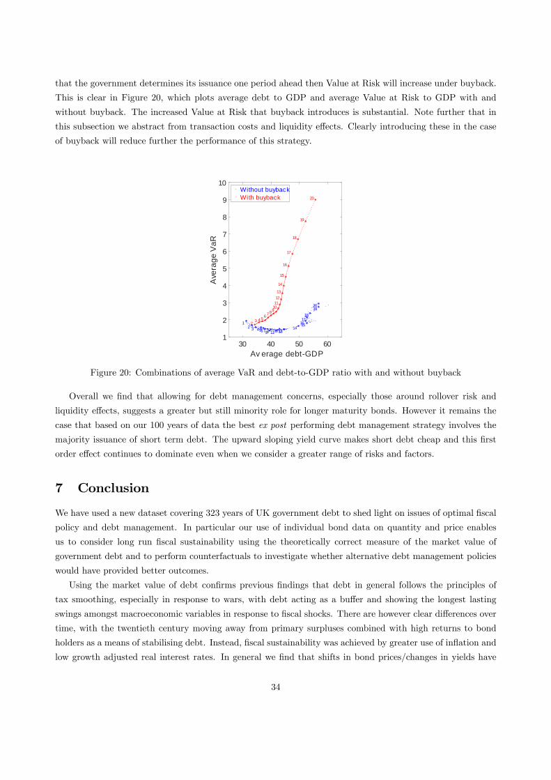
that the government determines its issuance one period ahead then Value at Risk will increase under buyback.
This is clear in Figure 20, which plots average debt to GDP and average Value at Risk to GDP with and
without buyback. The increased Value at Risk that buyback introduces is substantial. Note further that in
this subsection we abstract from transaction costs and liquidity effects. Clearly introducing these in the case
of buyback will reduce further the performance of this strategy.
Av erage debtGDP30 40 50 60
Ave
rage
VaR
1
2
3
4
5
6
7
8
9
10
12 3 4567 89 1011 1213
14151617
181920
2 3 4 56 78910111213
14
15
16
17
18
19
20
Without buybackWith buyback
Figure 20: Combinations of average VaR and debt-to-GDP ratio with and without buyback
Overall we find that allowing for debt management concerns, especially those around rollover risk and
liquidity effects, suggests a greater but still minority role for longer maturity bonds. However it remains the
case that based on our 100 years of data the best ex post performing debt management strategy involves the
majority issuance of short term debt. The upward sloping yield curve makes short debt cheap and this first
order effect continues to dominate even when we consider a greater range of risks and factors.
7 Conclusion
We have used a new dataset covering 323 years of UK government debt to shed light on issues of optimal fiscal
policy and debt management. In particular our use of individual bond data on quantity and price enables
us to consider long run fiscal sustainability using the theoretically correct measure of the market value of
government debt and to perform counterfactuals to investigate whether alternative debt management policies
would have provided better outcomes.
Using the market value of debt confirms previous findings that debt in general follows the principles of
tax smoothing, especially in response to wars, with debt acting as a buffer and showing the longest lasting
swings amongst macroeconomic variables in response to fiscal shocks. There are however clear differences over
time, with the twentieth century moving away from primary surpluses combined with high returns to bond
holders as a means of stabilising debt. Instead, fiscal sustainability was achieved by greater use of inflation and
low growth adjusted real interest rates. In general we find that shifts in bond prices/changes in yields have
34

contributed little to fiscal sustainability and that long bonds rarely offer much in the way of fiscal insurance
and even when they do it is of limited quantity. Long bonds are particularly expensive during financial crises
as falls in interest rates lead to large capital gains for long bonds and high returns to investors, and so high
funding costs for governments. This has been strikingly apparent in the most recent financial crisis with the
market value of debt ending our sample at its highest premium relative to face value for the whole 323 years.
Because the yield curve is normally upwards sloping and because long bonds offer little in the way of fiscal
insurance, our counterfactual analysis suggests that over the 20th century the UK government would have
been better off issuing just three year bonds. Had they done so, debt in 2016 would have been lower by around
28% of GDP. The first order effect of lower yields dominates any second order considerations regarding the
volatility and covariance of long bond prices. This is a function both of the size of the term premium but also
the limited and intermittent ability of long bonds to provide fiscal insurance outside of certain sub-periods.
To reduce the outperformance of short bonds in our 100 year counterfactuals requires either increasing
their yields or introducing additional risks. If liquidity effects are an important feature of government bond
markets then this has the potential to make a focus on issuing just short bonds expensive. However these
liquidity effects themselves need to be large and are less a disadvantage of short bonds per se but of any
issuance strategy based around only a few maturities. Focusing on rollover risk does suggest reducing the role
of short bonds but even in this case short bonds should form a majority of the portfolio. We find little role for
debt managers using leverage or buyback - in both cases rollover risk is increased by an order of magnitude
and if transaction costs are important then these will be costly to implement. More importantly we find that
neither strategy enables the government to achieve a better debt-risk trade off then more simple policies.
These findings question the empirical relevance of the optimal debt management literature’s preference
for long bonds and also comes to critical conclusions on the UK’s practice in supporting the longest average
maturity government debt portfolio in the world. At the heart of these findings is a term premia that gives
a strong preference to short term debt and covariance properties of long run debt that provide only a limited
insurance role in an issuance strategy. Any explanation of why the government issues so many bonds of so
many different maturities and why the average maturity is so great will have to focus not on stochastic features
of the yield curve but on the nature of bond market microstructure and bond market specific risks which are
as yet ill-defined in the literature.
35
References
[1] Aiyagari, R., Marcet, A., Sargent, T. and J. Seppälä (2002) “Optimal Taxation without State Contingent
Debt”Journal of Political Economy 110, 6, 1220-1254
[2] Allen, W. (2012) “Government Debt Management and Monetary Policy in Britain since 1919” Cass
Business School Working Paper 02/12
[3] Angeletos, G.-M. (2002) “Fiscal policy with non-contingent debt and optimal maturity structure”, Quar-
terly Journal of Economics, 117, 1105-1131
[4] Barro, R.J. (1979) “On the determination of the Public Debt”, Journal of Political Economy, 87, 5, 940-71
[5] Barro, R.J. (2003) “Optimal Management of Indexed and Nominal Debt”, Annals of Economics and
Finance, 4, 1-15
[6] Buera, F. and J.P. Nicolini (2004) “Optimal Maturity of Government Debt with Incomplete Markets”,
Journal of Monetary Economics, 51, 531-554
[7] Breedon, F. and P. Turner (2016) “On the transactions costs of quantitative easing”, BIS Working Paper
No.571
[8] Brewer, J. (1989), The Sinews of Power: War, Money and the English State 1688-1783, Cambridge
University Press
[9] Butkiewicz, J.L. (1983) “The market value of outstanding government debt : Comment”, Journal of
Monetary Economics, 11, 3, 373-379
[10] Capie, F. (2014) “British Financial Crises in the Nineteenth and Twentieth Centuries” in Dimsdale and
Hotson British Financial Crises Since 1825, Oxford University Press
[11] Clark, G. (2001) “Debt, Deficits and Crowding Out : England 1727-1840”European Review of Economic
History 5(3) 403-435
[12] Cochrane, J. (1988) “How big is the random walk in GDP?”Journal of Political Economy, 96, 5, 893-920
[13] Crafts, N. (2016) “Reducing High Public Debt Ratios : Lessons from UK Experience”Fiscal Studies 37,2
201-223
[14] Dickson, P.G.M. (1967) The Financial Revolution in England : A Study in the Development of Public
Credit 1688-1756, Routledge
[15] Faraglia, E., Marcet, A., and A. Scott (2010) “In Search of a Theory of Debt Management”, Journal of
Monetary Economics, 57, 821-836
[16] Faraglia, E., Marcet, A., Oikonomou, R. and A. Scott (2016) “Long Term Government Bonds”, London
Business School mimeo
[17] Faraglia, E., Marcet, A., Oikonomou, R. and A. Scott (2017) “The Long and the Short of It”, London
Business School mimeo
36

[18] Guibaud S., Nosbusch, Y. and D. Vayanos (2013) “Bond Market Clienteles, the Yield Curve, and the
Optimal Maturity Structure of Government Debt”, Review of Financial Studies, 26, 1914-61
[19] Hall, G. and T.J. Sargent (2010) “Interest Rate Risk and Other Determinants of Post WW-II U.S.
Government Debt/GDP Dynamics”, NBER Working Paper, No. 15702
[20] Hall, G. and T.J. Sargent (2011) “Interest Rate Risk and Other Determinants of Post WW-II U.S.
Government Debt/GDP Dynamics”, American Economic Journal : Macroeconomics, 3,192-214
[21] H.M. Treasury (2016) Debt Management Report 2016-17
[22] Klovland, J.T. (1994) “Pitfalls in the Estimation of the Yield on British Consols, 1850-1914”, Journal of
Economic History, 54, 1, 164-187
[23] Lou, D., Yan, H. and J. Zhang (2013) “Anticipated and Repeated Shocks in Liquid Markets”, Review of
Financial Studies, 26, 8, 1891-1912
[24] Lustig, H., Sleet, C. and S. Yeltekin (2009) “Fiscal hedging with nominal assets” Journal of Monetary
Economics, 55, 710-727
[25] Macauley, T.B. (1899) “History of England Vol 8”The Complete Writings of Lord Macauley Ch.19 p.70
[26] Marcet, A. and A. Scott (2009) “Debt and deficit fluctuations and the structure of bond markets”, Journal
of Economic Theory 144(2) 473-501
[27] Neal, L. (1990) The rise of financial capitalism: international capital markets in the Age of Reason,
Cambridge University Press
[28] Nosbusch, Y. (2008) “Interest Costs and the Optimal Maturity Structure of Government Debt”, Economic
Journal, 118, 477-498
[29] O’Brien, P.K. (2008) “Mercantilist Institutions for the Pursuit of Power with Profit: The Management
of Britain’s National Debt 1756-1815” in F.P. Caselli (ed) Government Debts and Financial Markets in
Europe, Routledge
[30] Reinhart, C.M. and K. Rogoff(2009) This Time is Different: Eight Centuries of Financial Folly, Princeton
University Press
[31] Schwarz, A.J. (1986) “Real and pseudo financial crises”in F. Capie and G. Wood (eds.) Financial Crises
and the World Banking System London, Macmillan 11-31
[32] Smith, A. (1776) The Wealth of Nations Book Five, Ch III “Of Public Debt”
[33] Song, Z. and H. Zhu (2016) “QE Auctions of Treasury Bonds”MIT mimeo
[34] Waggoner, D.F. (1997), “Spline methods for extracting interest rate curves from coupon bond prices”,
Federal Reserve Bank of Atlanta Working Paper, 97-10
37