managing multiple knowledge sources in constraint-based
TRANSCRIPT

Purdue UniversityPurdue e-Pubs
ECE Technical Reports Electrical and Computer Engineering
4-1-1994
Managing multiple knowledge sources inconstraint-based parsing of spoken languageMary P. HarperPurdue University School of Electrical Engineering
Randall A. HelzermanPurdue University School of Electrical Engineering
Follow this and additional works at: http://docs.lib.purdue.edu/ecetr
This document has been made available through Purdue e-Pubs, a service of the Purdue University Libraries. Please contact [email protected] foradditional information.
Harper, Mary P. and Helzerman, Randall A., "Managing multiple knowledge sources in constraint-based parsing of spoken language"(1994). ECE Technical Reports. Paper 185.http://docs.lib.purdue.edu/ecetr/185
TR-EE 94-16 APRL 1994

Abstract
In this paper, we describe a system which is capable of utilizing a variety of knowledge
sources to select the most appropriate parse for a spoken sentence. These knowledge sources
include syntax, semantics, and contextual information. We discuss one way to utilize contextual
information when determining a parse for a sentence. Our definition of a context is defined by
which computer application we wish to interact with, where our system is capable of interfacing
with two or more applications, each with a fixed vocabulary, syntax, and semanltics. The user
is able to interact through a single interface which uses contextual knowledge not only to parse
the query, but also to select the appropriate application to interact with. This birings us closer
to developing a more general purpose interface for multiple applications.


1 Introduction
Developing a computer model capable of understanding language (either spoken or text-based) is a
difficult problem, made more difficult by the ambiguity inherent in natural languages. Ambiguity
appears in many forms, including word recognition, syntax, word-sense, ambiguity of reference,
and quantifier scope. Because they are often interrelated, resolving each type of ambiguity often
requires that the others be handled at the same time. For example, the syntactic representation of
a sentence can constrain the possible antecedents for a referential noun phrase, while the antecedent
of a pronoun can also constrain the sentence's syntactic representation [5].
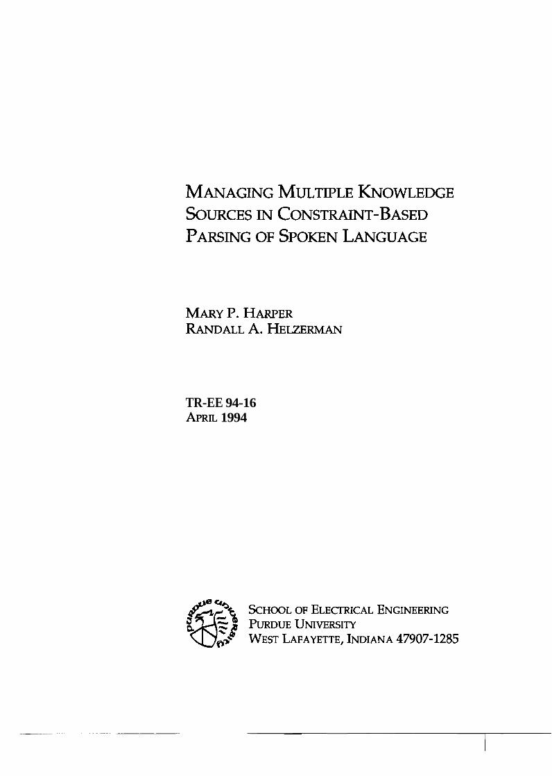
One way to resolve ambiguity is to utilize a wide variety of knowledge so.urces. The knowl-
edge sources commonly used in speech understanding are shown in Figure 1. Effective use of
multiple knowledge sources plays a key role in human spoken language understanding. It is, there-
fore, likely that advances in spoken language understanding will require effective utilization of this
information1.
To utilize the variety of knowledge sources needed to disambiguate language, we have con-
structed a constraint-based system [6, 7, 271 which is an extension to Constraint Dependency
Grammar (CDG) parsing as defined by Maruyama [15, 16, 171. This system is; capable of propa-
gating a wide variety of constraints, including syntactic, lexical, semantic, proso~dic, and contextual
constraints. The central data structure for this system is a word graph augmented with parse
related information, called a spoken language constraint network (SLCN). An SLCN represents all
possible parses for the represented sentence hypotheses in a compact form, ant1 is operated on by
constraints.
One of the most difficult knowledge sources t o incorporate into a computer system is pragmatics.
Pragmatics is the use of language in context. Often pragmatics deals with aspects of communication
which go beyond the literal truth conditions of the sentence, as in speech acts. However, here we will
only consider how context can help disambiguate the meaning of a sentence and identify precisely
.which context applies for a particular utterance.
For the purposes of this paper, we equate context with the choice of a computer application.
As shown in Figure 2, a user's input is processed by the language processor which interfaces with
two or more applications, each defining its own context. The goal of this systenl is t o interact with
'Prosody can help a word recognizer to rule out word candidates with unlikely stress and duration patterns, but it can also impact syntactic and semantic modules. Therefore, we depict the prosody module as both a high-level and low-level knowledge source.
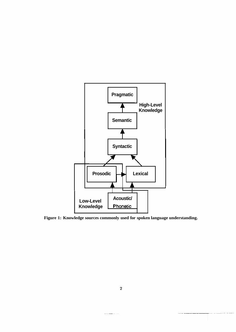
Figure 1: Knowledge sources commonly used for spoken language understanding.
Pragmatic
High-Level Knowledge
Semantic
Syntactic
Prosodic +b Lexical
I I I
Low-Level Knowledge
Acoustic/ phonetic
Language I .=Tr
Figure 2: A language interface to multiple computer applications.
the correct application given the user's spoken input. Initially, it analyzes a world graph of sentence
hypotheses provided by a speech recognizer using general syntactic and semantic. rules. Then, if the
utterance is still ambiguous, it utilizes context-specific constraints to further refine the analysis.
The system utilizes all of the knowledge sources it has access to in order to identify the correct
context. Also by identifying the correct context, the system should be able to further refine the
parse of the user's input. This synergy between syntax, semantics, and pragmaitics can be handled
quite effectively in our constraint-based system. This computer system, once capable of utilizing
multiple contexts within an evolving picture of what a sentence's parse, can be tlzought of as having
an imagination. Each hypothesis is subject to constraints which helps the computer t o disambiguate
the input syntactically and semantically while determining which context actuz~lly applies.
We begin our discussion by introducing constraint dependency grammars as defined by Maruyama
in section 2. Then in section 3, we describe how that algorithm is extended to process multiple
sentence hypotheses in a single constraint network. This same mechanism is utilized to handle
not only multiple sentence hypotheses with shared words, but also sentences with multiple parts
of speech, feature values, and contexts. We initially describe the mechanism for parsing multiple
sentences, and then describe how it can be used as a general mechanism for processing all ambiguity
inherent in a sentence, even the ambiguity of selecting the correct computer application with which

to interact.
2 The Theoretical Basis of the SLCN Parser
Our system uses Constraint Dependency Grammar (CDG) grammar, originally defined by Maruyama
[15, 16, 171, to process sentences. In the following subsections, we will describe the CDG grammar
formalism, the CDG parsing algorithm, and the benefits of a constraint-based system.
2.1 Elements of a CDG Grammar
Maruyama defines a CDG grammar as a four-tuple, ( C, R, L, C ), where:
C = a f i n i t e s e t of preterminal symbols, or l ex ica l categories. R = a f i n i t e s e t of uniquely named roles (or role- ids) = { r l , . . . , r p ) . L = a f i n i t e s e t of labels = ( 1 1 , . . . , l q ) . C = a constraint aet that an assignment A must aatiafy.
A sentence s = ~ 1 ~ 2 ~ 3 . . . w, is a string of finite length n and is an element of C*. All of the roles
in R are associated with every wi of s yielding n * p roles for the entire sentence. The sentence s is
said to be generated by the grammar G if there exists an assignment A which maps role values to
each of the n * p roles for s such that the constraint set C is satisfied. A role val.ue is an element of
the set L x {1,2,. . .,n,nil). In other words, it is a tuple consisting of a label fronn L and a modifiee,
where a modifiee can be the index of a word in the sentence or nil. Role values will be denoted in
the examples as label-rnodifiee. L(G) is the language generated by grammar G if and only if L(G)
is the set of all sentences generated by G. Note that the null string E has no roles and is always
generated by any grammar according to definition.
A constmint set is a logical formula in the form: 'd xl 2 2 . . . x, : role (and P1 P2 . . . P,),
where the xis range over all of the role values in the roles of s. Below is the definition of possible
components of a subformula P;':
Variables: XI, "2, . . . x,.
Constants: elements and subsets of C U L U R U {nil, 1, 2, . . ., n), where n corresponds to
the number of words in a sentence.
Access Functions:
(pos x) returns the position of the word for role value x.
2Maruyama uses an infix notation; whereas, we use a prefix notation throughout this paper.
(rid x) returns the role-id for role value x.
(lab x) returns the label for role value x.
(mod x) returns the position of the modifiee for role value x.
(cat i) returns the category (i.e., the element in C) for the word3 in position i.
Predicate symbols:
(eq x y) returns true if x = y, false otherwise.
(gt x y) returns true if x > y and x, y E Integers, false otherwise4.
(It x y) returns true if x < y and x, y E Integers, false otherwise.
(elt x y) returns true if x E y, false otherwise.
Logical Connectives:
(& p q) returns true if p and q are true, false otherwise.
(V p q) returns true if p or q is true, false otherwise.
(not p) returns true if p is false, false otherwise.
Each Pi in C must be of the form (if Antecedent Consequent), where Antecede~zt and Consequent
are predicates or predicates joined by the logical connectives. A CDG grammar has two associated
parameters, degree and arity. The degree of a grammar G is the size of R. The arity of the grammar
corresponds to the maximum number of variables in the subformulas of C. To simplify the examples
in this section, we use a grammar with a degree of one, that is, with a single :role governor. The
governor role indicates the function a word fills in a sentence when it is governeld by its head word.
In our implemented grammars, we also use several needs roles (e.g, needl, needl2) to make certain
that a head word has all of the constituents it needs to be complete (e.g., a siingular count noun
needs a determiner to be a complete noun phrase). Maruyama has proven that is grammar requires
a degree and arity of at least two to be as expressive as a CFG.
To illustrate the use of CDG grammars, consider a very simple example grammar, GI = ( C1,
R1, L1, C1 ) in Figure 3, which has a degree of one and an arity of two5. A subformula Pi is called a
unary constmint if it contains one variable and a binary constmint if it contains two. For example,
U-1, U-2, and U-3 are unary constraints because they contain a single variable, and B-1 is a binary
constraint because it contains two variables.
'Maruyama uses the access function word rather than cat, though the function accesses the category of the word. 'For example, (gt 1 nil) is false, because nil is not an integer. 'The constraints in this grammar were chosen for simplicity, not to exemplify constraints for a wide coverage
grammar.
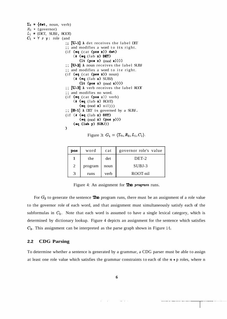
= {dot , noun, verb) R1 = {governor) L1 = {DET, SUBJ , ROOT) C1 = V z y : role (and
; ; [U-l] A det receives the l a b e l DET ; ; and modifies a word t o i ts r i g h t . ( i f (eq (ca t (pos x)) dot)
(& (eq ( lab x) DET) ( I t (poe x) (mod x) 1)
;; [U-2) A noun receives the l abe l SUBJ ; ; and modifies a word t o i t e r i g h t . ( i f (eq (ca t (poe x)) noun)
(& (eq ( lab x) SUBJ) ( I t (pos X) (mod x) 1)
; ; [U-31 A verb receives the l abe l ROOT ; ; and modifies no word. ( i f (eq (ca t (poe x ) ) verb)
(& (eq ( lab x) ROOT) (eq (mod x) n i l ) ) )
; ; [B-l] A DET is governed by a SUBJ . ( i f (& (eq ( lab x) DET)
(eq (mod x) (pos y ) ) ) (eq ( lab y) SUBJ))
1
Figure 3: GI = (XI, R1, L1, C1).
Figure 4: An assignment for The program runs.
For G1 to generate the sentence The program runs, there must be an assignment of a role value
to the governor role of each word, and that assignment must simultaneously satisfy each of the
subformulas in C1. Note that each word is assumed to have a single lexical category, which is
determined by dictionary lookup. Figure 4 depicts an assignment for the sentence which satisfies
C1. This assignment can be interpreted as the parse graph shown in Figure 14..
governor role's value
DET-2
SUBJ-3
ROOT-nil
POS
1
2
3
2.2 CDG Parsing
To determine whether a sentence is generated by a grammar, a CDG parser must be able to assign
at least one role value which satisfies the grammar constraints to each of the 1% + p roles, where n
word
the
program
runs
ca t
de t
noun
verb
node 1
( E l * WT-1, DET-2, WTJ, ruw* suaci, ~UBJ-2 suw~.
ROOld, ROOT-1. W - 2 , RooTJ)
(WT- DET-1, DET-2, DETJ. WAMI, wab1, ww-2 SUw4,
Rooria, RooT-I, W T - 2 Ra3T-a)
S U M , SUW-I. SUW-2 suw-a,
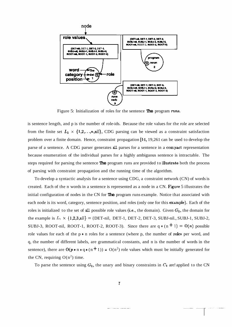
Figure 5: Initialization of roles for the sentence The program rtrns.
is sentence length, and p is the number of role-ids. Because the role values for the role are selected
from the finite set L1 x {1,2,. . .,n,nil), CDG parsing can be viewed as a constraint satisfaction
problem over a finite domain. Hence, constraint propagation [14, 19,261 can be used to develop the
parse of a sentence. A CDG parser generates all parses for a sentence in a com:pact representation
because enumeration of the individual parses for a highly ambiguous sentence is intractable. The
steps required for parsing the sentence The program runs are provided to illustra,te both the process
of parsing with constraint propagation and the running time of the algorithm.
To develop a syntactic analysis for a sentence using CDG, a constraint network (CN) of words is
created. Each of the n words in a sentence is represented as a node in a CN. Fig.ure 5 illustrates the
initial configuration of nodes in the CN for The program runs example. Notice that associated with
each node is its word, category, sentence position, and roles (only one for this ex;tmple). Each of the
roles is initialized to the set of all possible role values (i.e., the domain). Given GI, the domain for
the example is L1 x {1,2,3,nil) = {DET-nil, DET-1, DET-2, DET-3, SUBJ-nil., SUBJ-1, SUBJ-2,
SUBJ-3, ROOT-nil, ROOT-1, ROOT-2, ROOT-3). Since there are q * (n + 1) = O(n) possible
role values for each of the p * n roles for a sentence (where p, the number of ~aoles per word, and
q, the number of different labels, are grammatical constants, and n is the number of words in the
sentence), there are O(p * n * q * (n + 1)) = O(n2) role values which must be initially generated for
the CN, requiring O(n2) time.
To parse the sentence using GI, the unary and binary constraints in C1 are! applied to the CN

Figure 6: The CN after the propagation of U-1 for the sentence The pnymm runs.
to eliminate the role values from the roles of each word which are incompatible with C1. For a
sentence to be grammatical, each role in each word node must contain at least lone role value after
constraint propagation.
The unary constraints are applied to each of the roles in the sentence to eliminate the role
values incompatible with each word's role in isolation. To apply the first unary constraint (i.e.,
U-1, shown below) to the network in Figure 5, each role value for every role is examined to ensure
that it obeys the constraint.
;; [U-1] A det receives the label DET ;; and modifies a word t o i t s r ight . ( i f (eq (cat (pos x ) ) dot)
(& (eq (lab x) DET) ( I t (pos X) (mod x ) ) ) )
If a role value causes the antecedent of the constraint to evaluate to TRUE ant1 the consequent to
evaluate to FALSE, then that role value is eliminated. Figure 6 shows the remaining role values
after U-1 has been applied to the CN in Figure 5.
Maruyama requires that each subformula in a constraint set be evaluated in constant time.
Because of this restriction, each constraint can only contain access functions and predicates that
operate in constant time (e.g., access functions and predicates like those defined in Section 2.1).
So when the unary constraint U-1 is applied to O(n2) role values, it requires O(n2) time.
To further eliminate role values which are incompatible with the categories of the words in the
example, the remaining unary constraints (i.e., U-2 and U-3) are applied to the CN in Figure 6,
producing the network in Figure 7. Given that the number of unary constrain~ts in a grammar is
a grammatical constant denoted as ku, the time required to apply all of the unary constraints in a
grammar is O(ku * n2).
The binary constraints determine which pairs of role values can legally coexist. To keep track

Figure 7: The CN after the propagation of all the unary constraints.
w Figure 8: The CN after unary constraint propagation and before binary constraint propagation.
of pairs of role values, arcs connect each role to all other roles in the network, and each arc has an
associated arc matriz, whose row and column indices are the role values associated with the two
roles. The elements of an arc matrix can either be a 1 (indicating that the two role values which
index the element are compatible) or a 0 (indicating that the role values cannot simultaneously
exist). Initially, all entries in each matrix are set to 1 , indicating that the two role values are
initially compatible. Since there are (ny) = O(n2) arcs required in the CN, and each arc contains
a matrix with O((q * (n + I ) ) ~ ) = O(n2) elements, the time to construct the arcs and initialize
the matrices is O(n4). Figure 8 shows the matrices associated with the arcs before any binary
constraints are propagated. Unary constraints are usually propagated before preparing the CN for
binary constraints because they eliminate impossible role values from each role, and hence reduce
the dimensions of the arc matrices.
Binary constraints are applied to the pairs of role values indexing each of the arc matrix entries.
When a binary constraint is violated by a pair of role values, the entry in the matrix indexed by

Figure 9: The CN after B-1 is propagated.
those role values is set to zero. The binary constraint, B-1, ensures that a DET is governed by a
SUBJ:
; [B-I] A DET is governed by a SUBJ. (if ( k (eq (lab x) DET)
(eq (mod x) (pos y 1) (eq (lab y) SUBJ))
After the application of this constraint to the network in Figure 8, the element indexed by the role
values x=DET-3 and y=ROOT-nil for the matrix on the arc connecting the governor roles for the
and runs is set to zero, as shown in Figure 9. This is because the must be governed by a word with
the label SUBJ, not ROOT. Since the constraint must be applied to O(n4) pairs of role values, the
time to apply the constraint is 0(n4). Given that the number of binary constraints in a grammar
is a grammatical constant denoted as b, the time required to apply all of the binary constraints
in a grammar is O(kb * n4).
Following the propagation of binary constraints, the roles of the CN could still contain role
values which are incompatible with the parse for the sentence. To determine whether a role value
is still supported for a role, each of the matrices on the arcs incident to the role must be checked
to ensure that the row (or column) indexed by the role value contains at least a single 1. If any
arc matrix contains a row (or column) of 0s for the role value, then that role value cannot coexist
with any of the role values for the second role and so is removed from the list of legal role values for
the first role. Additionally, the rows (or columns) associated with the eliminated role value can be
removed from the arc matrices attached to the role. The process of removing any rows or columns
containing all zeros from arc matrices and eliminating the associated role valueis from their roles is

I N I {i, j , . . .) is the set of all roles, with I NI = p * n. I
Notation
( 4 j )
Meaning
An ordered pair of roles. 7
L
Li
{a, b, . . .) is the set of role values, with ILI = q * n
{ala E L and (i, a) is admissible) 1 ( a )
a E Li is supported by b E Lj after binary constraint propagation iff the element indexed by [a, b] in the matrix for arc (i, j ) contains a 1.
( 4 a) An ordered pair of role i and role value a E Li. I M[i, a1
( j , b) E S[i, a] means that role value a a t role i and b at j are simultaneously admissible.
M [ i , a] = 1 indicates that the role value a is not admissible for (and has already been eliminated from) the arc joining roles i and j .
E
I Counter[(;, j ) , a] I The number of role values in L, which are compatible with a in Li. 1
All role pairs (i, j) .
Figure 10: Data structures and notation for the CN arc consistency algoritl~m (i.e., AC-4).
List
called filtering. Following binary constraint propagation any of the O(n2) role values may require
immediate filtering. However, filtering must also be applied iteratively since the elimination of a
role value from one arc could lead to the elimination of a role value from anoth~er arc.
The algorithm used for filtering a constraint network is known as arc consis.tency by constraint
satisfaction researchers. An optimal version of the algorithm, AC-4, was devel.oped by Mohr and
Henderson [18]. AC-4 builds and maintains several data structures, described in Figure 10, to
allow it to efficiently perform this operation. Figure 11 shows the code for iinitializing the data
structures, and Figure 12 contains the algorithm for eliminating inconsistent role values from the
domains. This filtering algorithm requires O(ea2), where e is the number of arcs, and a is the size
of the domain [18]. In the case of CDG parsing, e = ("y), and the domain size is n * q, so the
running time of the filtering step is O(n4) [15, 161.
If the role value a at role i is compatible with b at role j, then a supports b. To keep track of
how much support each role value a has, the number of role values in L j which are compatible with
a in L; are counted, and the total is stored in Counter[(i, j), a]. The algorithm must also keep track
A queue of arc support to be deleted. I

1. List:=$; 2. for i~ N do 3. for a E Li do 4. begin 5. M[i, a] := 0; 6. S[i, a] := 4; 7. end 8. for ( i , j) E E do 9. f o r b E L i d o 10. begin 11. Total=O; n12. for b E Lj do 13. if Rd(i, a, j, b) then 14. begin 15. Total=Total+l; 16. S[j, b] := S[j, b] + {(i, a)); 17. end 18. if Total=O then 19. begin 20. M[i, a] = 1; 21. List:=List ~ { ( i , a)); 22. Li = Li - {a); 23. end 24. else 25. Counter[(i, j), a] =Total; 26. end
Figure 11: Construction of data structures for CN arc consistency (i.c?., AC-4).
of which role values that role value a supports by using S[i, a], which is a set o-i arc and role value
pairs. For example, S[i, a] = {(j, b), (j,c)) means that a in L; supports b and c in Lj. If a is ever
invalid for L; then b and c will loose some of their support. This is accomplished by decrementing
Counter[(j, i), b] and Counter[(j, i), c]. For CN arc consistency, if Counter[(i, j ) , a ] becomes zero, a
is automatically be removed from L;, because that would mean that a is impossible in any sentence
parse. When a role value a E i is found to be unsupported, the algorithm places the ordered pair
( 2 , a ) on List. When (i, a ) is popped off List in the procedure in Figure 12, additional role values
may loose support and be placed on List.
Consider how filtering is applied to the CN in Figure 9. The matrix assolciated with the arc
connecting the and runs contains a row with a single element which is a zero. Because DET-3
cannot coexist with the only possible role value for the governor role of runs, it cannot be a legal
member of the governor role of the, and so (1, det-3) is placed on List, and det-3 is eliminated as
a role value for node 17s governor role. When the role value is eliminated from all arcs associated
with the role, filtering is complete and the resulting CN is depicted in Figure 13.
After all the constraints are propagated across the CN and filtering is l~erformed, the CN
provides a compact representation for all possible parses. Syntactic ambiguity is easy to spot in

1. while List not empty do 2. begin 3. choose (j, b) from List and remove (j, b) from List; 4. for (i, a) E Slj, b] do 5. begin 6. Counter[(i, j ) , a]=Counter[(i, j ) , a] - 1 ; 7. if Counter[(;, j ) , a] = 0 and M [i, a] = 0 then 8. begin 9. List:=List U{(i, a)); 10. M [ i , a]=l; 11. Li = Li - {a) 12. end 13. end 14. end Figure 12: Algorithm to enforce CN arc consistency (i.e., AC-4).
Figure 13: The CN after filtering.

Word = The Cat = det
G = DET-2
Figure 14: The parse graph for the CN in Figure 13.
the CN since some of the roles in an ambiguous sentence contain more than a single role value.
If multiple parses exist, we can propagate additional constraints to further reline the analysis of
the ambiguous sentence, or we could just enumerate the parses contained in the CN by using
backtracking search. For highly ambiguous grammars, the process of enumerating all possible
parses is intractable, making incremental disambiguation a more attractive option. The parse trees
in a CN are precedence graphs, which we call parse graphs, and they consist of a compatible set of
role values (given the arc matrices) for each of the roles in the CN. The modifiees of the role values,
which point t o the words they modify, form the edges of the parse graph. Ou-r example sentence
has an unambiguous parse graph given GI, shown in Figure 14.
Below we list the steps in the CDG parsing algorithm and their associated running times:
1. Constraint network construction prior to unary constraint propagation: O(n2)
2. Unary constraint propagation: O(k, * n2)
3. Constraint network construction prior t o binary constraint propagation: 0 (n4 )
4. Binary constraint propagation: O(kb * n4)
5. Filtering (arc consistency): O(n4)

2.3 Benefits of a Constraint-based Approach
There are many benefits to using a constraint based parser, with the primary one being flexibility.
When a traditional context-free grammar (CFG) parser generates a set of ambiguous parses for a
sentence, it cannot invoke additional production rules to further prune the analyses. In contrast,
in CDG parsing, the presence of ambiguity can trigger the propagation of additional constraints to
further refine the parse for a sentence. A core set of constraints that hold universally can be propa-
gated first, and then if ambiguity remains, additional, possibly context dependent, constraints can
be used. We have already developed semantic constraints which are used to eliminate parses with
semantically anomalous readings from the set represented in the constraint network [7]. Additional
knowledge sources are quite easy to add given the uniform framework providedl by constraints, as
we demonstrate in this paper.
Tight coupling of prosodic [3] and semantic rules with CFG grammar rules typically increases
the size and complexity of the grammar and reduces its understandability. Semantic grammars
have been effective for limited domains, but they do not scale up well to larger systems [I]. The
most successful modules for semantics are more loosely coupled with the syntactic module (e.g., in-
terleaved or postprocessing). The constraint-based approach represents a loosely-coupled approach
for combining a variety of knowledge sources. It differs from a blackboard appro'ach in that all con-
straints are applied using the uniform mechanism of constraint propagation. Hence, the designer
does not need to create a set of functionally different modules and worry about their interface with
the other modules. Constraint propagation is a uniform method which allows us to focus on the
best way to order the sources of information impacting comprehension.
The set of languages accepted by a CDG grammar is a superset of the set of languages which
can be accepted by CFGs. In fact, Maruyama [15,16] is able to construct CDG grammars with two
roles (degree = 2) and two variable constraints (arity = 2) which accept the sa~me language as an
arbitrary CFG converted to Griebach Normal form. We have also devised an algorithm to map a
set of CFG production rules into a CDG grammar. This algorithm does not assume that the rules
are in normal form, and the number of constraints created is O(G). In addition, CDG can accept
languages that CFGs cannot, for example, anbncn and ww, (where w is some string of terminal
symbols). There has been considerable interest in the development of parsers for grammars that are
more expressive than the class of context-free grammars, but less expressive tha~n context-sensitive
grammars [12, 24, 251. The running time of the CDG parser compares quite favorably to the
running times of parsers for languages which are beyond context-free. For example, the parser for
tree adjoining grammars (TAG) has a running time of O(n6).
CFG parsing has been parallelized by several researchers. For example, Kositraju's method [13]
using cellular automata can parse CFGs in O(n) time using O(nZ) processors. However, achieving
CFG parsing times of less than O(n) has required more powerful and less impleinentable models of
parallel computation than used by [13], as well as significantly more processors. Ruzzo's method
[22] has a running time of O(logz(n)) using a CREW P-RAM model (Concurrent Read, Exclusive
Write, Parallel Random Access Machine), but requires O(n6) processors to achieve that time bound.
In contrast, we have devised a parallelization for the single sentence CDG parser [9, 81 which uses
O(n4) processors to parse in O(k) time for a CRCW P-RAM model (Concurrent; Read, Concurrent
Write, Parallel Random Access Machine), where n is the number of words in the sentence and
k, the number of constraints, is a grammatical constant. Furthermore, this algorithm has been
simulated on the MasPar MP-1, a massively parallel SIMD computer. The MP-1 supports up to
16K Cbit processing elements, each with 16KB of local memory. The CDG algorithm on the MP-1
achieves an O(k+log(n)) running time by using 0(n4) processors. By comparison, the TAG parsing
algorithm has also been parallelized, and operates in linear time with O(n5) processors [2:L].
To parse a free-order language like Latin, CFGs require that additional rilles containing the
permutations of the right-hand side of a production be explicitly included in the grammar [20].
Unordered CFGs do not have this combinatorial explosion of rules, but the recognition problem
for this class of grammars is NP-complete. A free-order language can easily be handled by a CDG
parser because order between constituents is not a requirement of the grammatical formalism.
Furthermore, CDG is capable of efficiently analyzing free-order languages because it is does not
have to test for all possible word orders.
In summary, CDG supports a framework which is more expressive and flexible than CFGs,
making it an attractive alternative to traditional parsers. It is able to utilize a variety of different
knowledge sources in a uniform framework to incrementally disambiguate a sentence's parse. The
algorithm also has the advantage that is is efficiently parallelizeable.
3 Parsing Spoken Sentences with Constraints
The output of a hidden-Markov-model-based speech recognizer is often a list of ithe most likely sen-
tence hypotheses (i.e., an N-best list) where parsing can be used to rule out the impossible sentence

hard
2 3 4 6 7 8 19
Figure 15: Multiple sentence hypotheses can be represented in a single word graph.
hypotheses. CDG constraints can be used to parse single sentences in a CN; however, individually
processing each sentence hypothesis provided by a speech recognizer is inefficient since many sen-
tence hypotheses are generated with a high degree of similarity. An alternative representation for
a list of similar sentence hypotheses is a word graph or lattice of word candida~tes which contains
information on the approximate beginning and end point of each word. A word graph represents a
disjunction of all possible sentence candidates that the speech recognizer provides.
Word graphs are typically more compact and more expressive than N-best s,entence lists. In an
experiment in [27], word graphs were constructed from three different lists of sentence hypotheses.
The word graphs provided an 83% reduction in storage, and in all cases, they encoded more
possible sentence hypotheses than were in the original list of hypotheses. In one case, 20 sentence
hypotheses were converted into a word graph representing 432 sentence hypotheses. Figure 15
depicts a word graph containing four sentence hypotheses which was constructedl from two sentence
hypotheses: *It's hard to recognizes speech and It's hard to wreck a nice beach. If the spoken
language parsing problem is structured as a graph processing problem, then the constraints used
to parse individual sentences would be applied to a word graph of sentence hypotheses, eliminating
from further consideration all those hypotheses that are impossible given the constraints.
We have adapted the CDG constraint network to handle the multiple sentence hypotheses
stored in a word graph, calling it a Spoken Language Constraint Network (SLCN). The input to
the parser is a word graph like the one shown in Figure 15. Each word node in the word graph
contains information on the beginning and end point of the word's utterance, represented as an
integer tuple (b, e), with b < e. The tuple is more expressive than the point scheme used for CNs
and requires modification of some of the access functions and predicates defined for the CN scheme.
It's a
It's
hard nitx
hard
to beach wreck
to recognizes speech

Notice that nodes that can be adjacent t o one another are joined by directed edges. A sentence
hypothesis must include one word node from the beginning of the utterance, one word node from
the end of the utterance, and these two word nodes must be connected by a path of edges. The
number of sentence hypotheses represented by a graph of n nodes can be exponential in the size
of n. The goal of our system is t o utilize constraints t o eliminate as many impossible sentence
hypotheses as possible, and then t o select the best remaining sentence hypothesis (given the word
probabilities given by the recognizer).
To apply constraints t o the word graph, each word node must be annotated with a set of roles.
Then each role for each'word node is assigned a set of role values, requiring O(n2) time, where n
is the number of word candidates in the graph. Unary constraints are applied t o each of the role
values in the network, and like CNs, require O(k, * n2) time.
Some of the constraint access functions and predicates must be adapted for SLCN parsing. For
example, the access functions ( ~ o s x) and (mod x) now return a tuple (b, e) which describes the
position of the word associated with the role value x. Hence, the equality predicate is extended t o
test for equality of intervals (e.g., (eq (1,2) (1,2)) should return true). Also, the Iless-than predicate,
(It ( b l , e l ) (b2, e2)), returns true if e l < b2, and the greater than predicate, (gt ( b l , e l ) (b2, e2)),
returns true if b l > e2. One additional change is needed t o accommodate multiple words over the
same time interval. Recall that in CN parsing a word node has a unique category and position.
Hence, t o access the category associated with a role value, Maruyama would use the function (cat
(pos i)), where (pos i) returns the position of the role value, and its category is accessed by using
the position of the word in the sentence. For an SLCN, it is not always po!jsible t o determine
the category for a role value by using the position of the word in the sentence because some word
nodes share the same position. We handle this by allowing the role values t o keep track of their
part of speech, not just the position of their word node. Hence, the constraints in Figure 3 must
be rewritten so that the access function cat operates on a role value rather than on a word node
addressed by its position. For example, U-1 is rewritten as follows:
;; [U-11 A det receives the label DET ;; and modifies a word t o i t s r ight . ( i f (eq (cat x) det) ;; use (cat x) rather than (cat (pas x ) )
(L (eq ( lab x) DET) ( I t (pos X ) (mod x ) ) ) )
The preparation of the SLCN for the propagation of binary constraints is similar t o that for
a CN. All roles within the same word node are joined with an arc as in a CIS\; however, roles in

Figure 16: Multiple sentence hypotheses can be parsed simultaneously by propagating constraints over an SLCN rather than individual CNs.
different word nodes are joined with an arc if and only if they can be memb'ers of at least one
common sentence hypothesis (i.e., they are connected by a path of directed ed.ges). To construct
the arcs and arc matrices for an SLCN, it suffices to traverse the graph from beginning to end
and string arcs from each of the current word node's roles to each of the preceding word node's
roles (where a node precedes a node if and only if there is a directed edge fro:m the preceding to
the current node) and to each of the roles that the preceding word nodes' roles have arcs to. For
example, there should be an arc between the roles for recognizes and speech in Figure 16 because
they are located on a path from the beginning to the end of the sentence *It's hard to recognizes
speech. However, there should not be an arc between the roles for wreck and n:cognizes since they
are not found in any of the same sentence hypotheses. After the arcs for the SLCN are constructed,
the arc matrices are constructed in the same manner as for a CN. The time required to construct
the SLCN network in preparation for binary constraint propagation is O(n4) because there may
be up O(nZ) arcs constructed, each requiring the creation of a matrix with 0(1a2) elements. Once
the SLCN is constructed, binary constraints are applied to pairs of role values ,associated with arc
matrix entries (in the same manner as for the CN), requiring O(kb* n4) time, where n is the number
of word candidates.
Filtering in an SLCN is complicated because the limitation of one word's function in one sentence
hypothesis should not necessarily limit that word's function in another sentence hypothesis. For
example, consider the SLCN depicted in Figure 16. Even though all the role values for to would

Figure 17: The AND/OR graph for the CDG parsing algorithm.
be disallowed by the third person singular verb recognizes, those role values cannot be eliminated
since they are supported by wreck, an infinitive verb. The SLCN filtering a1gorit:hm cannot disallow
role values that are allowed by at least one sentence in the network, in contrast to CN filtering
algorithm. Hence, we must modify the CN filtering algorithm to accommodate word graphs. We
have developed an algorithm to achieve arc consistency in an SLCN by using the properties of the
directed acyclic graph representing the word network to filter role values that can never appear
in any parse [6, 101. This algorithm, described in the next section, operates correctly with single
sentences as well as word graphs.
3.1 SLCN Arc Consistency
When we create a constraint network representing multiple alternative senteilce hypotheses, we
have changed the logical meaning of the constraint network significantly. A CN can be thought of
as an AND/OR graph such that the values assigned to the roles of a word account for the only
OR nodes in the graph, as shown in Figure 17. Hence, for a sentence to have a parse, every role
in the CN must have a least one role value after filtering. A CN with this semantics is said to be
an: consistent if and only if for every pair of roles i and j , each role value in the domain of i has at
least one role value in the domain of j for which they both satisfy the binary cconstraints.
On the other hand, an SLCN is constructed from a parse graph containing multiple sentence
candidates, some with shared word nodes. Figure 18 depicts a simple SLCN with two roles con-
structed from a word graph. An OR node is required at the top level of the graph to represent
the contribution of various word nodes to the different sentence hypotheses in .the SLCN. Though
the individual sentence hypotheses are not indicated individually in the SLCN (this would require
exponential space in some cases), the logical presence of the OR node must be captured by the arc
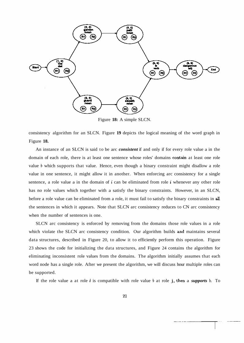
Figure 18: A simple SLCN.
consistency algorithm for an SLCN. Figure 19 depicts the logical meaning of the word graph in
Figure 18.
An instance of an SLCN is said to be arc consistent if and only if for every role value a in the
domain of each role, there is at least one sentence whose roles' domains contain at least one role
value b which supports that value. Hence, even though a binary constraint might disallow a role
value in one sentence, it might allow it in another. When enforcing arc consistency for a single
sentence, a role value a in the domain of i can be eliminated from role i whenever any other role
has no role values which together with a satisfy the binary constraints. However, in an SLCN,
before a role value can be eliminated from a role, it must fail to satisfy the binary constraints in ad
the sentences in which it appears. Note that SLCN arc consistency reduces to CN arc consistency
when the number of sentences is one.
SLCN arc consistency is enforced by removing from the domains those role values in a role
which violate the SLCN arc consistency condition. Our algorithm builds andl maintains several
data structures, described in Figure 20, to allow it to efficiently perform this operation. Figure
23 shows the code for initializing the data structures, and Figure 24 contains the algorithm for
eliminating inconsistent role values from the domains. The algorithm initially assumes that each
word node has a single role. After we present the algorithm, we will discuss hour multiple roles can
be supported.
If the role value a at role i is compatible with role value b at role j, then a supports b. To
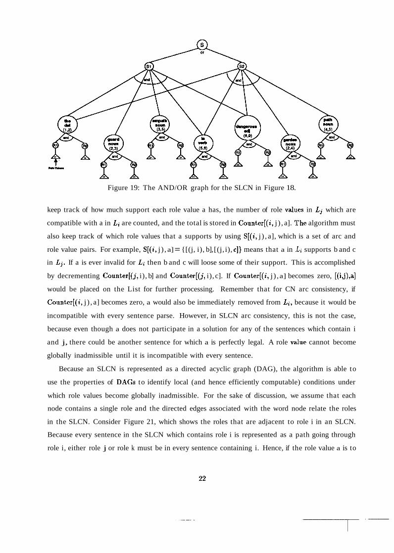
Figure 19: The AND/OR graph for the SLCN in Figure 18.
keep track of how much support each role value a has, the number of role values in Lj which are
compatible with a in L; are counted, and the total is stored in Counter[(i, j ) , a]. The algorithm must
also keep track of which role values that a supports by using S[(i, j ) , a], which is a set of arc and
role value pairs. For example, S[(i, j ) , a] = {[(j, i), b], [(j, i), c]) means that a in L; supports b and c
in Lj. If a is ever invalid for L; then b and c will loose some of their support. This is accomplished
by decrementing Counter[(j, i), b] and Counter[(j, i), c]. If Counter[(i, j ) , a] becomes zero, [(ij),a]
would be placed on the List for further processing. Remember that for CN arc consistency, if
Counter[(i, j ) , a] becomes zero, a would also be immediately removed from L;, because it would be
incompatible with every sentence parse. However, in SLCN arc consistency, this is not the case,
because even though a does not participate in a solution for any of the sentences which contain i
and j, there could be another sentence for which a is perfectly legal. A role value cannot become
globally inadmissible until it is incompatible with every sentence.
Because an SLCN is represented as a directed acyclic graph (DAG), the algorithm is able to
use the properties of DAGs to identify local (and hence efficiently computable) conditions under
which role values become globally inadmissible. For the sake of discussion, we assume that each
node contains a single role and the directed edges associated with the word node relate the roles
in the SLCN. Consider Figure 21, which shows the roles that are adjacent to role i in an SLCN.
Because every sentence in the SLCN which contains role i is represented as a path going through
role i, either role j or role k must be in every sentence containing i. Hence, if the role value a is to

Notation
(4 j )
a E Li is supported by b E Lj after binary constraint propagation iff the element indexed by [a, b] in the matrix for arc (i, j ) contains a 1.
Meaning
An ordered pair of roles.
I 1
N
L
Li
I [(i, j) , a1 I An ordered pair of a role pair (i, j) and a role value a E Li. I
-
{i, j, . . .) is the set of all roles, with IN1 = p * n.
{a, b, . . .) is the set of role values, with ILI = q * n
{ala E L and (i, a) is admissible)
M[(i, j) , a] = 1 indicates that the role value a is not admiz3sible for (and has already been eliminated from) all sentences containing i and j.
All role pairs (i, j ) such that there exists a sentence which contains both i and j . We distinguish (i, j ) from ( j , i) for the purposes of arc consistency, even though there is a single undirected arc joining two roles in the network.
[(j, i), b] E S[(i, j) , a] means that role value a at role i and b at j are simultaneously admissible.
Next-edge;
Prev-edge;
Counter[(;, j) , a]
If a directed edge from i to j exists in E, then (i, j ) is a member of the set.
If a directed edge from j to i exists in E, then ( j , i) is a
The number of role values in Lj which are compatible
'rev-Support[(', j) , 'I (i, k) E Prev-Support[(i, j) , a] means that a is admissible in every sentence which contains i, j , and k.
Next-Su~~ort[( i , j)! '1 (i, k) E Next-Support[(i, j) , a] means that a is admissible in every sentence which contains i, j, and k.
Local-Prev-Support(i, A set of elements (i, j ) such that (j , i) E Prev-edgei and a is compatible with a t least one of j's role values.
Local-Next-Support(i,
Figure 20: Data structures and notation for the SLCN arc consistency algorithm.
A set of elements (i, j ) such that (i, j ) E Next-edgei and a is compatible with a t least one of j's role values.
I
List A queue of arc support to be deleted.

Local-Prev-Support I,a = { l,n ,(i,m)) ~oc.1-~xt-~upport[i.a{ = {[i,j)i
Figure 21: Local-Prev-Support and Local-Next-Support for an example SLCN. The solid directed lines represent the SLCN edges and the dotted directed lines represent the arcs. We use the directionality of the arcs to represent the fact that an arc matrix associated with an arc is used in two ways. For example, n's role values support i's role values, but also i's role values support n's. The sets indicate that the role value a is allowed for every sentence which contains n, m, and j, but is disallowed for every sentence which contains k.
reniain in L;, it must be compatible with a t least one role value in either Lj or Lk. Also, because
either n or m must be contained in every sentence containing i, if a is to remain. in L;, it must also
be compatible with at least one role value in either L, or L,.
In order to track this dependency, two sets are maintained for each role value a at role i, Local-
Next-Support (i, a) and Local-Prev-Support (i, a). Local-Next-Support (i, a) is a set of ordered role
pairs (i, j ) such that (i, j ) E Next-edge;, and there is at least one role valu,e b E Lj which is
compatible with a. Local-Prev-Support(i, a) is a set of ordered pairs (i, j ) such that ( j , i ) E Prev-
edge; and there is at least one role value b E Lj which is compatible with a. VVhenever one of i's
adjacent roles, j, no longer has any role values b in its domain which are compatible with a, then
(i, j ) should be removed from Local-Prev-Support(i, a) or Local-Next-Support(i, a), depending on
whether the edge is from j to i or from i to j, respectively. If either Local-Prev-Support(i,a) or
Local-Next-Support(i, a) becomes the empty set, then a is no longer a part of an!{ solution, and may
be eliminated from L;. In Figure 21, the role value a is admissible for the sentence containing i and
j, but not for the sentence containing i and k. If because of additional constraints, the role values
in j become inconsistent with a on i, (i, j ) would be eliminated from Local-Next-Support(a,i),
leaving an empty set. In that case, a would no longer be supported by any sentence.
The algorithm can utilize similar conditions for roles which may not be directlly connected to i by
Next-edge; or Prev-edge,. Consider Figure 22. Suppose that the role value a at role i is compatible
with a role value in Lj, but it is incompatible the role values in L, and L,, then it is reasonable to
eliminate a for all sentences containing both i and j , because those sentences would have to include

( i t ~ )
Figure 22: If Next-edgej = {(j, x), ( j , y)) and S[(i, x), a] = 4 and S[(i, y), a] = 4 , then a is inadmis- sible for every sentence containing both i and j.
either role x or y. To determine whether a role value is admissible for a set of sentences containing
i and j, we calculate Prev-Support[(i, j ) , a] and Next-Support[(i, j) , a] sets. Next-Support[(i, j) , a]
includes all (i, k) arcs which support a in i given that there is a directed edge between j and k,
and (i, j ) supports a. Prev-Support[(i, j ) , a] includes all (i, k) arcs which support a in i given that
there is a directed edge between k and j, and (i, j) supports a. Note that Prev-Support[(i, j) , a]
will contain an ordered pair (i, j ) if (i, j ) E Prev-edgej , and Next-Support[(i, j:), a] will contain an
ordered pair (i, j ) if ( j , i) E Next-edgej. These elements are included because the edge between roles
i and j is sufficient to allow j's role value to support a in the sentences containing i and j. Dummy
ordered pairs are also created to handle cases where a role is at the beginning or end of a network:
when (s ta r t , j ) E Prev-edgej, ( i ,s tar t ) is added to Prev-support[(i, j) ,al , and when ( j ,end) E
Next-edgej, ( i ,end) is added to Next-support[(i, j ) , a ] . This is to prevent a role value from being
ruled out because no roles precede or follow it in the SLCN. Figure 23 shows the Prev-Support,
Next-Support, Local-Next-Support, and Local-Prev-Support sets that the initi,alization algorithm
creates for some role values in a simple example SLCN.
To illustrate how these data structures are used in SLCN arc consistency (see Figure 24),
consider what happens if initially [(I, 3), a] E List for the SLCN in Figure 23. [( L,3), a] is placed on
the list to indicate that the role value a in role 1 is not supported by any of the role values associated

1. List:=4; 2. E := {(i, j)l3a E C : i, j E a A i # j A i, j E N); 3. for ( i , j) E E d o 4. f o r a E L i d o 5. begin 6. M[(i, j), a] := 0; 7. Prev-Support[(i, j), a] := 4; Next-Support[(;, j), a] := 4; 8. Local-Prev-Support(i, a) := 4; Local-Next-Support(i, a) := 4; 9. S[(i, j), a1 := 4; 10. end 11. for ( i , j ) E E d o 12. f o r a E L i d o 13. begin 14. Total:=O; 15. for b E Lj d o 16. if Rd(i, a, j, b) then 17. begin 18. Total:=Total+l; 19. s[( j , i), bl := S[(j, i), bl u {[(i,j), a]); 20. e n d 21. if Total=O then 22. begin 23. M[(i, j),a] := 1; 24. List:=List U{[(i, j), a]); 25. e n d 26. Counter[(;, j), a]:=Total; 27. Prev-Support[(i, j), a] := {(i, z)l(i, z) E E (z, j) E Prev-edgej)
U{(i, j)l(i, j ) E Prev-edgej) U {(i, start)l(start, j) E Prev-edgej); 28. Next-Support[(i, j), a] := {(i, z)l(i, z) E E (j , z ) E Next-edgej)
U{(i, j)l(j, i) E Next-edgej ) U {(i, end)l(j, end) E Next-edgej); 29. if (i, j ) E Next-edgei t h e n 30. Local-Next-Support(;, a):=Local-Next-Support(i, a) U{(i, j)); 31. if ( j , i) E Prev-edgei t h e n 32. Local-Prev-Support(;, a):=Local-Prev-Support(;, a) U {(i, j)); 33. end
Next-Sup- 1 2 a = 1,3)) Next-Sup{l:3~:al=Ih.end)) Next-Sup 1 2 b = 1 3))
Next-Supl[l:31:b = fh:end)) Next-Sup 2 1 c = 2 1),(2 3)) Next-Sup'[2:31:~ = 
1. while List # d do beg& '
choose [ ( j , i ) , b] from List and remove it from List; for [ ( i , j ) , a1 E S [ ( j , 9, bl do
begin Counter[(;, j ) , a]:=Counter[ i , j ) , a] - 1; if Counter[(;, j ) , a] = 0 A M ( i , j ) , a] = 0 then
begin \
List:=List U{[( i , j ) , a] ) ; M [ ( i , j ) ,a] := 1;
end end
for ( j , z ) E Next-Support[(j, i ) , b] do begin
Prev-Support[(j, z ) , b]:=Prev-Support[(j, z ) , b] - { ( j , i ) ) ; if Prev-Support[(j, z ) , b] = 4 A M [ ( j , z ) , b] = 0 then
begin List:=List U{[ ( j , z ) , b] ) ; M [ ( j , z ) , b] := 1;
end end
for ( j , z ) E Prev-Support[(j, i ) , b] do begin
Next-Support[(j, z ) , b]:=Next-Support[(j, z ) , b] - { ( j , i ) ) ; if Next-Support[(j, z ) , b] = 4 M [ ( j , z ) , b] = 0 then
begin List:=List U{[ ( j , z ) , b] ) ; M [ ( j , z ) , b] := 1;
end end
if ( j , i ) E Next-edgej then Local-Next-Support(j, b):=Local-Next-Support(j, b) - { ( j , i ) ) ;
if Local-Next-Support(j, b) = 4 then begin
Lj := Lj - {b) ; for ( j , z ) E Local-Prev-Support(j, b) do
if M [ ( j , z ) , b ] = 0 then begin
List:=List U{[ ( j , z ) , b]); M [ ( j , z ) , b] := 1;
end end
if ( i , j ) E Prev-edgej then Local-Prev-Support(j, b):=Local-Prev-Support(j, b) - { ( j , i ) ) ;
if Local-Prev-Support(j, b) = 4 then begin
Lj := Lj - {b) ; for ( j , z ) E Local-Next-Support(j, b) do
if M [ ( j , z ) , b] = 0 then begin
List:=List ~ { [ ( j , z ) , b]); M [ ( j , z ) , b] := 1;
end end
end
Figure 24: Algorithm to enforce SLCN arc consistency.
with role 2. When that value is popped off List, it is necessary to remove [(I, 3), a]'s support
from all S[(3, I ) , x] such that [(3, I ) , x] E S[(1, 3), a] by decrementing for each x, Counter[(3,l), x]
by one. If the counter for any [(3, I ) , x] becomes 0, and the value has not already been placed
on the List, then it is added for future processing. Once this is done, it is nlecessary to remove
[(I, 3), a]'s influence on the SLCN. To handle this, we examine the two sets Prev-Support[(l, 3), a] =
{(1,2), (1,3)) and Next-Support[(l, 3), a] = ((1, end)). Note that the value (1, end ) in Next-
Support [ ( l ,3) , a] and the value (1,3) in Prev-Support[(l, 3), a], once eliminated from those sets,
require no further action because they are dummy values. However, the value (1,2) in Prev-
Support[(l, 3), a] indicates that (1,3) is a member of Next-Support[(l, 2), a], and since a is not
admissible for (1,3), (1,3) should be removed from Next-Support [(1 ,2) , a], leaving an empty set.
Note that because Next-Support[(l, 2), a] is empty and assuming that M[(1,2) ., a] = 0, [(I, 2), a] is
added to List for further processing. Next, (1,3) is removed from Local-Next-Support(1, a), but
that set is non-empty. During the next iteration of the while loop [(I, 2), a] is popped from List.
When Prev-Support[(l, 2), a] and Next-Support[(l, 2), a] are processed, Next-Snpport[(l, 2), a] = 4 and Prev-Support[(l, 2), a] contains only a dummy, which is removed. When (1,2) is removed from
Local-Next-Support(1, a) , the set becomes empty, so a is no longer compatible with any sentence
containing role 1 and can be eliminated from further consideration as a possible role value for role
1. Once a is eliminated from role 1, it is also necessary to remove the support of a E L1 from all role
values on roles that precede role 1, that is for all roles x such that (1, x) E Local-IPrev-Support(1, a).
Since Local-Prev-Support(1,a) = {( l , s t a r t ) ) , and start is a dummy role, there is no more work
to be done.
In contrast, consider what happens if initially [(I, 2), a] E List for the SLCN in Figure 23. In
this case, Prev-Support[(l, 2), a] contains (1,2) which requires no additional work; whereas, Next-
Support [(I, 2), a] contains (1,3), indicating that (1,2) must be removed from Prev-Support[(l, 3), a]'s
set. After the removal, Prev-Support[(l, 3), a] is non-empty, so the sentence containing roles 1 and
3 still supports the role value a on 1. The reason that these two cases provide different results is
that roles 1 and 3 are in every sentence; whereas, roles 1 and 2 are only in one of them.
3.2 The Running Time and Correctness of SLCN Arc Consistency
The running time of the routine to initialize the SLCN arc consistency structures (in Figure 23)
is O(n4), and the running time for the algorithm which prunes labels that are not arc consistent
(in Figure 24) also operates in O(n4) time, where n is the number of word nodes in network. By

comparison, the running time for CN arc consistency is O(n4), assuming that there are n words in
a sentence. The proof of correctness of this algorithm is detailed in [lo, 111, but we will summarize
it below.
A role value is eliminated from a domain by SLCN arc consistency only if its Local-Prev-
Support or its Local-Next-Support set becomes empty. Therefore, we must shoar that a role value's
local support sets become empty if and only if that role value cannot participate in an SLCN
arc consistent solution. This is proven for Local-Next-Support (Local-Prev-!$upport follows by
symmetry). Observe that if a E L;, and it is incompatible with all of the roles which immediately
follow L; in the SLCN, then it cannot participate in an SLCN arc consistent solution. In line 32
in Figure 24, (i, j ) is removed from Local-Next-Support(i, a ) set only if [(i, j),cz] has been popped
off List. Therefore, we show that [(i, j ) , a ] is put on List, only if a E L; is inconnpatible with every
sentence which contains i and j, by induction on the number of iterations of the while loop.
For the base case, the initialization routine only puts [(i, j ) , a] on List if a E L; is incompatible
with every role value in L j (line 24 of Figure 23). Therefore, a E L; is in no solution for any sentences
which contain i and j. Assume the condition holds for the first k iterations of the while loop in
Figure 24, then during the (k+l)th iteration, tuples of the form [(i, j ) , a] for thce (k+l)th iteration
were put on List by line 9 in Figure 24 or by line 24 in Figure 23 (in which case a is no longer
compatible with any labels in Lj), line 18 in Figure 24 (in which case Prev-Support([(i, j ) , a]) = 4),
line 27 in Figure 24 (in which case Next-Support([(i, j ) , a]) = 4), or line 39 in Figure 24 (there is
no longer any Local-Next-Support for a). In any of these cases, a E L; is incompatible with every
sentence which contains i and j. We can therefore conclude that this is true for all iterations of
the while loop.
3.3 Multiple Roles in an SLCN
As shown in Figure 18, an SLCN can have more than a single role. In our initial development of
the SLCN arc consistency algorithm discussed in [6], we distinguished between1 two types of arcs:
intm-arcs, which are arcs joining roles within the same word node, and inter-arcs, which are arcs
joining roles across word nodes. The inter-arcs were processed in the same way as in the algorithm
in Figures 23 and 24, but the intra-arcs were handled differently. They seemed to require special
handling because if a role value is disallowed for role x by a role y within the same word node as z ,
then the role value must be eliminated from z. In this case, the elimination of the role value from
x is correct because every sentence containing the word node disallows the role value.

Figure 25: An SLCN with multiple roles compatible with our new algorithm.
Special handling of this case complicates the arc consistency algorithm; however, there is a
simpler way to accomplish precisely the same effect as the special case while using the simpler
algorithm shown in Figures 23 and 24. It simply involves setting up the SLCN in a slightly different
way than in Figure 18. The edges in the SLCN in Figure 18 relate the roles across nodes but not
roles within the same word node. If we assume that the roles within a word node are connected
by directed edges as in Figure 25, then the arc consistency algorithm in Figure 24 is sufficient for
SLCNs with more than a single role. Because there is a single linear list of roles within a word
node, they must appear in all the same sentences, and so if one role value is disallowed by one of
the roles in the linear list of roles, it will be eliminated from the role. This is because every sentence
containing the first role must also contain the other role (i.e., there are no alternative paths that
include both roles). Hence, we set up SLCNs with more than a single role as :shown in Figure 25
and use the simpler arc consistency algorithm described in this paper.
3.4 Lexical Ambiguity
Many words in the English language have more than a single part of speech. For example, the word
garden in Figure 25 can either be a noun or a verb. Maruyama's algorithm requires that a word
have a single part of speech, which is determined by dictionary lookup prior to the application of
the parsing algorithm. Since parsing can be used to lexically disambiguate a sentence, ideally, a
parsing algorithm should not require that a part of speech be known prior to piusing. In addition,

Figure 26: An SLCN with multiple parts of speech for some words.
lexical ambiguity, if not handled in a reasonable manner, can cause correctness and/or efficiency
problems for a parser [4, 61.
To handle lexically ambiguous words, we create a word node for each legal part of speech for a
word. These word nodes cannot appear in the same sentence hypotheses and sol are not connected
to each other by directed edges, and do not share arcs for binary constraints. For example, Figure
26 depicts an SLCN which supports multiple parts of speech for several different word nodes. This
method of handling multiple parts of speech within our constraint parsing algorithm requires the
use of the SLCN arc consistency algorithm described in this paper.
Multiple parts of speech can be handled in a CN algorithm (as discussed bjr Harper and Helz-
erman in [6]) by creating separate role values for each part of speech within the same word node,
where it becomes the responsibility of the role value to keep track of its lexical category. How-
ever, the approach uses more space and requires an additional constraint wh~en compared with
the method described in this paper. Role values associated with two different I-oles within a word
node should not be allowed to support each other if they do not correspond to the same part of
speech. Hence, we must propagate a binary constraint which zeros out the entries of all intra-arc
arc matrices that are indexed by role values corresponding t o different parts of speech. By using
an SLCN t o handle lexical ambiguity, the roles of the word nodes corresponding to different parts
of speech cannot appear in any common sentences and so are not connected by arcs, eliminating
the wasted space and the need for an additional constraint.

3.5 Feature Analysis
Lexical features, like number, person, and case, are used in many natural language parsers to enforce
subject-verb agreement, determiner-head noun agreement, and case requirements for pronouns.
This information can be very useful for disambiguating parses for sentences or for eliminating
impossible sentence hypotheses, hence our parser supports them.
Many times, even if a word is not lexically ambiguous, it can have ambiguity in the feature
information associated with the word. For example, the noun fish can take the number/person
feature value of third person singular or third person plural. It is important associate a single
feature value with each role value which is being tested for number agreement with another word's
role values. Because our parser utilizes only unary and binary constraints, role values with feature
value ambiguity can only be tested pairwise for consistency, and yet the feature values associated
with one word in a valid parse must often be compatible with more than one word in the sentence.
For example, if we store sets of features with a node when we parse the sentence *a fish eat, it is
easy to ensure that a and fish agree in number and person by using a binary constraint, and that
fish and eat agree, but without using ternary constraints, there is no way to ensure that a, fish,
and eat have jointly compatible feature values. Furthermore, there is no guarantee that ternary
constraints (or for that matter n-ary constraints, for any prespecified n) are sufficient to ensure
that the parser rejects sentences that are ungrammatical because of inc~mpat~ible feature values
(e.g., *The fish which are eating swims).
In order to enforce feature value compatibility across a set of words which must jointly agree
on a feature value in our parsing algorithm, word nodes should be duplicated (along with their
role values and arc matrices) and assigned a single feature value for the feature being tested by
a constraint, not a set of features. A naive and computationally expensive vvay to achieve this
end is t o initially duplicate each node so that all of the possible combinations of feature values are
covered. Fortunately, there is a better alternative; when the parser is propagating a constraint with
a particular feature test, a node with multiple values for that feature can be duplicated and assigned
one of the feature values, and then that constraint containing the feature test can be applied to its
role values, eliminating many of them before other types of feature constraints are propagated. A
grammar writer can order constraints in a constraint file in such a way that role value duplication is
minimized. For example, by placing pure phrase structure constraints before constraints containing
feature tests, syntactically eliminated role values will not have to be duplicated and tested against

I scenic \
Figure 27: A word graph provided to our system by the speech recognizer.
the feature constraints. Given this strategy, the running time of the parser with feature constraints
is comparable to the running time of the parser without feature tests.
In the next section, we illustrate how our system parses a word graph provided by a speech
recognizer. This example shows how node splitting is used to propagate syntactic feature constraints
in the presence of feature value ambiguity.
3.6 A Parsing example
To parse a sentence, our parser requires a grammar designer to specify the grammar parame-
ters, write and test constraints consistent with the grammar parameters, and design a grammar-
appropriate lexicon. Assume that a grammar is needed to parse the word graph provided by our
speech recognizer shown in Figure 27.
The grammar designer provides a file containing the grammar parameters to the parser. This
file provides information needed to check constraints for good form and to create the constraint
network. Figure 28 depicts an example of a grammar parameter file for a simple grammar to parse
our example. Notice that in addition to categories, roles, and labels, there is ;a label-table which
restricts labels by part of speech and role id, a set of grammar features restricting the feature values
for each feature type, and a feature-table restricting the the legal feature types for each part of
speech.
Our parser uses the feature-table to check constraints and dictionary entries for good form. It
uses the label-table to restrict the possible labels for each role using the category of the word and
its role id. In practice, the table reduces the number of role values in the initial1 SLCN by a factor
of five to seven, and eliminates the need to propagate some unary constraints. Even though this

; A l i s t of the l ega l pa r t s of speech
(categories adj noun verb propernoun)
; A l i s t of r o l e names f o r the grammar
( ro les governor needs)
; A l i s t of l ega l l abe l s f o r the grammar
( labels root obj adj nounmod s blank)
; A l a b e l t ab le f o r r e s t r i c t i n g the domains given ; par t of speech and r o l e name.
( label- table (governor (noun noun-mod obj) (propernoun nounaod ob j ) (verb root) (adj ad j ) )
(needs (noun blank) (propernoun blank) (verb s ) (adj blank) 1)
; A l is t of l ega l fea ture types and possible values
(grarrrarleatures (number 1s 2s 3s l p 2p 3p) (subcat dobj) (sem-type sign p re t ty c i t y a i r- t ransfer show))
; A f ea tu re t ab le indicating the possible values f o r ; each fea tu re type associated with a pa r t of speech ; and i t s defaul t value i f none i s specified.
(f eature-table (adj (sea-type p re t ty [ 1 ) ) (noun (sea-type sign a i r- t ransfer [ 1 )
(number 3s 3p C3sl)) (propernoun (number 3s 3p C3sl)
(sem-type c i t y C 1 ) ) (verb (number 1s 2s 3s l p 2p 3p C3s1)
(subcat dob j ) (sem-type show C 1 ) ) )
Figure 28: A grammar parameter file for a simple example grammar.

(display (category noun (number 3s) (sem-type sign))
(category verb (number i s 2s lp 2p 3p) (subcat dob j ) (ser-type show)))
( f l i g h t (category noun (number 3s) (sea-type air-transf er) ) )
( f l i g h t s (root~rord f l i g h t ) (category noun (number 3p) ) ) )
(Phoenix (category propernoun (number 3s) (sen-type c i ty ) ) )
(scenic (category adj (sem-type pretty)))
Figure 29: A dictionary for parsing our example.
does not improve the asymptotic running time of the algorithm, it does decrease the actual running
time of the CDG algorithm (and the size of the SLCN).
The dictionary for our simple -example is described next. The lexicon mus:t specify all of the
words that can appear in a sentence. It is represented as a list of word entries, where each word
entry is a list headed by the associated word along with other important information. Each word
entry includes information on its legal parts of speech. In addition, syntactic and semantic features
are stored for each part of speech of a word. The lexicon for our example appears in Figure 29. This
lexicon stores information about noun number, verb number, semantic type, and subcategorization.
The word flights inherits features that are not mentioned in its entry from its soot form flight.
Given the grammar parameters, our system constructs the SLCN in Figure 30 from the word
graph in Figure 27 by looking up information on each word in the dictionary. Ntotice that there are
two roles for each word node, governor (i.e., G) and needs (i.e., N), and that twto nodes are created
for the word display because it has two possible parts of speech. All remaining features are initially
stored as sets on the word node. The role values assigned to each role are restricted to those that
are allowed by the label-table (and the restriction that no word ever modifies itself).
The constraints for our grammar are shown in Figure 31. Application of the unary constraints
over the SLCN in Figure 30 eliminates many of the role values, as shown in Figure 32. To apply
binary constraints, it is necessary to create arcs (and their corresponding arlc matrices) joining
those roles that can appear in at least one common sentence hypothesis. D r a ~ ~ i n g all of the arcs
would clutter the picture, so we will only depict those that are pertinent to pinpointing the parse
of the sentence. However, the reader should be aware that no arcs join the roles of the noun form
of display with the verb form of that word or the roles of scenic with the roles of Phoenix, because
they cannot appear in the same sentence hypotheses. Figure 33 depicts the state of the matrices

Figure 30: An SLCN constructed from the word graph in Figure 27.
that are affected by the binary constraints. All other matrices contain only ones. Notice that
we have numbered the roles in the SLCN. These numbers will allow us to discuss Prev-Support,
Next-Support, Local-Prev-Support, and Local-Next-Support sets when filtering; is applied next.
After the propagation of binary constraints, we must apply the filtering algorithm. First, the
preprocessing procedure in Figure 23 is invoked to examine all of the arc matrices associated with
the arcs and determine how the role values for each role are supported by elements associated with
the roles they share an arc with. If a role value a E i is not supported by an!y of the role values
associated with the role values of j, then the item [(i, j) ,a] is placed on List. 'The procedure also
calculates the Prev-Support, Next-Support, Local-Prev-Support, and Local-Next-Support sets for
each role value. Once this preprocessing step is complete, the arc consistency procedure in Figure
24 loops until all items on List have been processed. As items on List are processed, new items
can be inserted onto List.
After the preprocessing procedure has been executed, List contains the following items: [(9,6),
obj-(3,5)], [(9,8), obj-(3,5)], [(9,2), obj-(1,3)], [(7,2), obj-(1,3)], and [(4,5), s-(:1,5)]. For example,
the presence of [(9,6), obj-(3,5)] on List indicates that the role value obj-(3,,5) in role 9 is not
supported by any of the role values associated with role 6.
Note that (9,8) and (9,6) are the only members of Local-Prev-Support(9, obj-(3,5)) and so once
[(9,6), obj-(3,5)] and [(9,8), obj-(3,5)] are processed by the arc consistency procedure in Figure 24,

UUARY COUSTRAIUTS: ; A r o l e value v i t h l a b e l root modifies nothing.
( i f (eq ( lab I) root) (eq (mod I) n i l ) )
; A r o l e value v i t h l a b e l blank modifies nothing.
( i f (eq ( l ab I) blank) (eq (mod I) n i l ) )
; A r o l e value v i t h l a b e l adj modifies a vord t o i t s r i g h t .
( i f (eq ( l a b I) adj ) ( I t (pos I) (mod I ) ) )
; A r o l e value v i t h l a b e l nounaod modifies a vord t o i t s r i g h t .
( i f (eq ( lab I) nounaod) ( I t (pos I) (mod I ) ) )
; A r o l e value v i t h l a b e l obj modifies a word t o i t s l e i t . ( i f (eq ( l a b I) obj)
( g t (pos I) (mod 11))
; A r o l e value v i t h l a b e l s modifies a vord t o i t s r i g h t .
( i f (eq ( l a b I) s ) ( I t (pea I) (mod 1 ) )
BIUARY COUSTRAIUTS: ; A r o l e value f o r a verb v i t h l abe l s needs an obj which ; it governs.
( i f (k (eq ( l a b I) s ) (eq ( r i d y) governor) (eq (mod I) (pos y) 1)
(k (eq ( l a b y) obj) (eq (mod y) (pos I ) ) ) )
; A r o l e value f o r a noun v i t h l abe l obj i s governed by an ; EI vhich needs it.
( i f (k (eq ( l ab I) obj) (eq ( r i d y) needs) (eq (mod 1 ) (pas y ) ) )
(k (eq ( l ab y ) 8) (eq (mod y) (pos I) 1) )
Figure 31: The unary and binary constraints for our example!.

Figure 32: The SLCN after unary constraint propagation.
Figure 33: The SLCN after binary constraint propagation.
Local-Prev-Support(9, obj-(3,5))'s set becomes empty indicating that obj-(3,5) is not a legal role
value in any sentence hypothesis, and so it can be removed from role 9. In addition, a l l of the arcs
attached to role 9 will eliminate their support for obj-(3,5), and determine whether the elimination
of that role value makes it possible to add new items onto List. When the algorithm eliminates
[(9,4), obj-(3,5)] from the SLCN, it notices that [(4,9), s-(3,5)] should also be added to the List
because the removal of obj-(3,5) causes s-(3,5) to become unsupported.
When [(4,9), s-(3,5)] is processed, the algorithm must eliminate s-(3,5)'s support support given
Prev-Support[(4,9), s-(3,5)] = {(4,8), (4,6)) and Next-Support[(4,9), s-(3,5)] == {(4,10)). This is
achieved by removing (4,9) from Next-Support[(4,8), s-(3,5)] = {(4,9)) and Next-Support[(4,6),
S-(3,5)] = {(4,9)), leaving both sets empty, causing [(4,8), s-(3,5)] and [(4,6), s-(3,5)] to be added
to List. It must also remove (4,9) from Prev-Support[(4,lO), s-(3,5)] = {(4,9)), causing [(4,10),
s-(3,5)] to be added to the List. When [(4,6), s-(3,5)] is processed, the algorithm adds [(4,5), s-(3,5)]
to the List, and when [(4,8), s-(3,5)] is processed, it adds [(4,7), s-(3,5)]. Because Next-Support(4,
s-(3,5)) = {(4,5), (4,7)), once these two items are processed, s-(3,5) can be deleted from node 4.
When the role value is eliminated, the algorithm is able to add [(7,4), obj-(1,,3)] to List. When
[(7,4), obj-(1,3)] and [(7,2), obj-(1,3)] have both been processed, Local-Prev-Sulpport(7, obj-(1,3)),
which initially was {(7,4), (7,2)), becomes empty and so obj-(1,3) can be eliminated from role 7.
When obj-(3,5) is deleted from role 9, it also causes a chain of events to eliminate blank-nil from
role 2 (since role 9 is in every sentence hypothesis containing role 2), thereby eliminating the only
role value from role 2. After additional processing, the role values on role 1 alre also eliminated,
leaving the word node for the noun form of display without any support. The word node can be
pruned from the SLCN under these circumstances.
Once filtering is complete, the SLCN is in the state shown in Figure 34. The network is still
ambiguous since it contains a verb with multiple number values and two paths through the network.
To restrict the number for the word display, we would propagate a number feature constraint
indicating that a command verb must agree with the second person pronoun, you. To propagate
this constraint, the word node would be split into five similar nodes with the ollly difference being
the value stored for the number feature. The arcs and arc matrices associated with the node would
also be duplicated. After node duplication, a constraint would be propagated r'equiring agreement
with the word you, which has a number feature of either second person singular or plural. This
constraint would eliminate all but two of the nodes for the verb, as shown in Figure 35. To
determine which of the four remaining sentence hypotheses is correct requires the use of additional
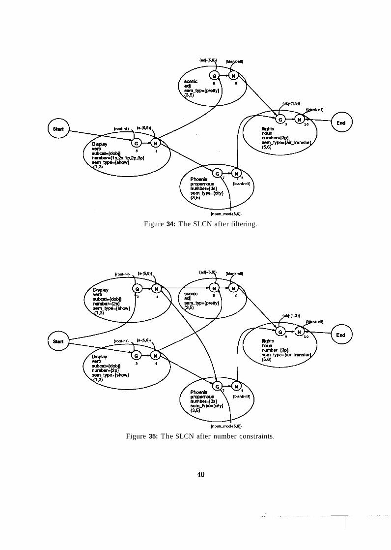
Figure 34: The SLCN after filtering.
(n~n-n-+(5,6)1
Figure 35: The SLCN after number constraints.

Figure 36: An SLCN after syntactic constraint propagation and filtering.
constraints.
Constraint propagation provides a uniform method for applying higher-level knowledge sources
to prune a word graph. Because the constraints for each knowledge source can be developed
independently, it is not as difficult t o add another knowledge source to our parser. In the next
section, we discuss the addition of semantic constraints.
3.7 Adding Semantic Constraints
Semantic features associated with the words in a dictionary can also be used to help disambiguate an
SLCN. To illustrate the use of semantic constraints, consider the SLCN in Figure 36, assuming that
syntactic constraints and syntactic feature constraints have been propagated, and filtering has been
performed. This SLCN represents two distinct sentence hypotheses: Show me flights to Atlanta and
Show me flights with Atlanta. Notice that the prepositions to and with are synte~ctically ambiguous
since they can either modify the noun flights or the verb show. In addition, t:he prepositions are
semantically ambiguous because they can fill a number of semantic functions i:n the sentence. By
using the semantic features in this sentence and two simple semantic constrai-nts, we are able to
disambiguate this network entirely. The constraints are shown in figure 37.
To propagate the semantic constraints, we must duplicate the word nodes associated with the
prepositions and assign each of them a unique semantic feature value, as sh.own in Figure 38.
The first constraint uses the semantic type of the head word in the object of the preposition to

; ; A location tha t is an object of a preposition modifies ;; a locat ive preposition.
( i f (& (eq ( lab x) ppab j ) (eq (mod x) (por y) (eq (ram-type x) locat ion)) ; ; Mote that a c i t y is a 10,cation.
(V (eq (sem-type y) t o l o c ) (eq (mom-type y) fromloc) (eq (sem-type y) a t l o c ) ) )
; ; A t o l o c preposition modifies a move-event . ( i f (and (V (eq (lab x) nqp )
(eq ( lab y) v q p ) ) (eq (mod x) (por y ) ) (eq (rem-type x) t o l o c ) )
(eq (sea-type y) move-event))
Figure 37: Semantic constraints for Look up stairs.
W-l)
Figure 38: An SLCN just prior to semantic constraint propgation.
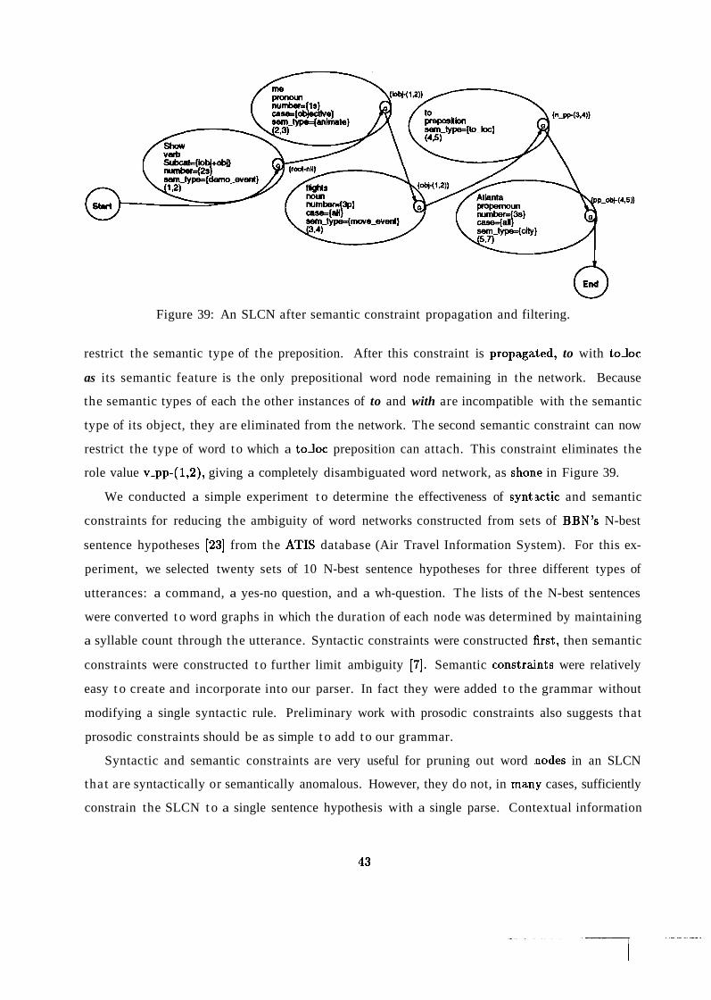
Figure 39: An SLCN after semantic constraint propagation and filtering.
restrict the semantic type of the preposition. After this constraint is propaga-ted, to with toloc
as its semantic feature is the only prepositional word node remaining in the network. Because
the semantic types of each the other instances of to and with are incompatible with the semantic
type of its object, they are eliminated from the network. The second semantic constraint can now
restrict the type of word to which a to loc preposition can attach. This constraint eliminates the
role value v-pp-(1,2), giving a completely disambiguated word network, as shone in Figure 39.
We conducted a simple experiment t o determine the effectiveness of syntiactic and semantic
constraints for reducing the ambiguity of word networks constructed from sets of BBN's N-best
sentence hypotheses [23] from the ATIS database (Air Travel Information System). For this ex-
periment, we selected twenty sets of 10 N-best sentence hypotheses for three different types of
utterances: a command, a yes-no question, and a wh-question. The lists of the N-best sentences
were converted t o word graphs in which the duration of each node was determined by maintaining
a syllable count through the utterance. Syntactic constraints were constructed first, then semantic
constraints were constructed t o further limit ambiguity [7]. Semantic constrajnts were relatively
easy t o create and incorporate into our parser. In fact they were added to the grammar without
modifying a single syntactic rule. Preliminary work with prosodic constraints also suggests that
prosodic constraints should be as simple t o add to our grammar.
Syntactic and semantic constraints are very useful for pruning out word inodes in an SLCN
that are syntactically or semantically anomalous. However, they do not, in man,y cases, sufficiently
constrain the SLCN t o a single sentence hypothesis with a single parse. Contextual information

represents an additional knowledge source that can be exploited to reduce the ambiguity in an
SLCN, as discussed in the next section.
3.8 Incorporating Pragmatic Constraints into SLCN Processin,g
Barwise and Perry [2] suggest that ambiguity of language is just another aspect of the efficiency of
language. The fact that an expression can be used in more than one way is just another feature
of that expression. Understanding an expression more fully comes at the cost of identifying the
context. If we can identify the context in which the sentence occurs (i.e., the situation), then we
can understand the expression more fully. Clearly to provide a general model ca~pable for smoothly
handling all the contexts that a human being can is beyond the scope of this paper. However,
we believe that by exploiting context as a feature of language, we can develop a constraint-based
system capable of utilizing this information.
For the purposes of this paper, we define a context as a computer application. A user can interact
with a language processor which interfaces with two or more applications as depicted in Figure 2.
Here the function of the natural language interface is to interact with the correct application given
the user's input. The process of parsing the input language should help to identify the correct
context, and the identification of the correct context should help to disambiguate the user's input.
As an example of the usefulness of context, assume our system receives the word graph from
our speech recognition module in Figure 27. Assume that there are three contexts, where c l
corresponds to an air travel database, c2 corresponds to a road map database, ,and c3 corresponds
to a program for designing signs. Our system constructs an SLCN from the w o ~ d graph by looking
up information on each word in the dictionary which stores the same informatioil as in our previous
example along with additional information about the contexts in which the word can occur. The
contextually augmented dictionary for our example is shown in Figure 40. Many words can be
shared across contexts, but some content words should appear in one context but not another. Just
knowing which contexts are supported by a word provides a useful clue for selecting the correct
context for an utterance.
The SLCN in Figure 41 is constructed from the word graph in Figure 27, assuming the grammar
parameter file in Figure 28 and the lexicon in Figure 40. As before, two nodes are created for the
word display because it has two possible parts of speech and all remaining features are initially
stored as sets on the word node, including contextual information.
By storing the allowable contexts with a word node, it is possible, without propagating even

(display (category noun (context c3) (number 3s) (sen-type s ign))
(category verb (context c i c2) (number is 2s i p 2p 3p) (subcat dobj ) (sem-t ype show) ) )
( f l i gh t (category noun (context c l c3) (number 3s) (sen-type air-transf e r ) ) )
( f l i gh t s (root-word f l i gh t ) (category noun (number 3 ~ ) ) ) )
(Phoenix (category propernoun (context c i c3) (number 3s) (sen-type c i t y ) ) )
(scenic (category adj (context c2) (sea-type pre t ty ) ) )
Figure 40: A contextually expanded dictionary for parsing our example.
Figure 41: An SLCN constructed from the word graph in Figure 27.

Figure 42: The SLCN pruned of words associated with context c2.
one constraint to eliminate a context from consideration. For a sentence to be a legal utterance
(given our restricted sense of context), it must have at least one common context across all word
nodes on the path. Also, for a context to be admissible, there must be a path from start to end
containing word nodes that support that context. For example, in Figure 41, context c2 is not
supported by the SLCN even before propagation of constraints. If a context is not supported by at
least one path through the network, then all word nodes that support only the disallowed context
can be immediately pruned, as shown in Figure 42. Notice that c2 is also elimjnated as a context
for the verb form of display.
The next step in processing a contextual SLCN is to propagate the context independent unary
and binary syntactic constraints in Figure 31 and filter the SLCN. Once this step is completed, the
SLCN is in the state depicted in Figure 43. Notice that following this, the wordl node for the noun
form of display is eliminated; therefore, context c3 is no longer supported and can be pruned from
the network.
Next we select a set of constraints for a context independent syntactic fea.ture to propagate.
For each node that has more than one value for the feature type, we duplicate the node and assign
it a single feature value. For example, if we propagate a number feature constraint, we would split
the node corresponding to the verb display, and propagate the constraint to limit the number of
command verb t o be 2s or 2p. Once this constraint is propagated, the network is in the state
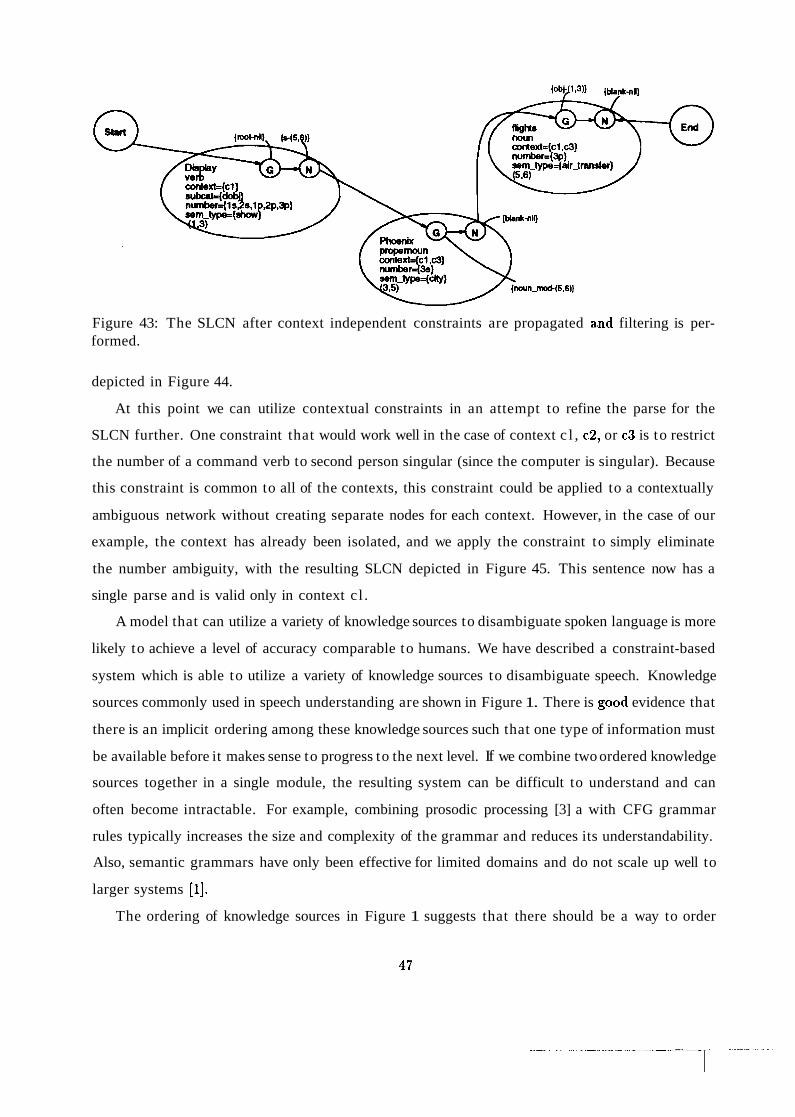
tobu1 9)) {blank-nl)
Figure 43: The SLCN after context independent constraints are propagated and filtering is per- formed.
depicted in Figure 44.
At this point we can utilize contextual constraints in an attempt to refine the parse for the
SLCN further. One constraint that would work well in the case of context c l , c2, or c3 is to restrict
the number of a command verb to second person singular (since the computer is singular). Because
this constraint is common to all of the contexts, this constraint could be applied to a contextually
ambiguous network without creating separate nodes for each context. However, in the case of our
example, the context has already been isolated, and we apply the constraint to simply eliminate
the number ambiguity, with the resulting SLCN depicted in Figure 45. This sentence now has a
single parse and is valid only in context c l .
A model that can utilize a variety of knowledge sources to disambiguate spoken language is more
likely to achieve a level of accuracy comparable to humans. We have described a constraint-based
system which is able to utilize a variety of knowledge sources to disambiguate speech. Knowledge
sources commonly used in speech understanding are shown in Figure 1. There is :good evidence that
there is an implicit ordering among these knowledge sources such that one type of information must
be available before it makes sense to progress to the next level. If we combine two ordered knowledge
sources together in a single module, the resulting system can be difficult to understand and can
often become intractable. For example, combining prosodic processing [3] a with CFG grammar
rules typically increases the size and complexity of the grammar and reduces its understandability.
Also, semantic grammars have only been effective for limited domains and do not scale up well to
larger systems [I].
The ordering of knowledge sources in Figure 1 suggests that there should be a way to order

Figure 44: The SLCN after context independent number feature constraints axe propagated and filtering is performed.
sem-typeSair-transfer]
Figure 45: The SLCN with a single sentence hypothesis in context c l .

constraints to limit the combinatorial explosion of managing all knowledge sources a t once. Below
we enumerate the steps of our algorithm:
1. Create an SLCN for the word graph by using a dictionary and eliminate i~n~ossible contexts.
2. Propagate context-independent syntactic unary constraints (no feature testing).
3. Construct arcs for binary constraint propagation.
4. Propagate context-independent syntactic binary constraints and filter the SLCN.
5. Loop for each set of syntactic feature type constraints:
Duplicate the nodes with more than a single value for that feature (role values, arcs,
and matrices too).
Propagate the constraints for that feature type.
Filter the network.
Eliminate impossible contexts.
6. For semantic feature constraints:
Duplicate the nodes with more than a single semantic feature value (role values, arcs,
and matrices too).
Propagate the semantic constraints.
Filter the network.
Eliminate impossible contexts.
7. For contextual constraints:
Duplicate the nodes with more than a single context,
Propagate the contextual constraints,
Filter the network.
Eliminate impossible contexts.
Depending on the number of contexts and the degree of sharing between contexts, we could
utilize a courser granularity for propagating context-specific constraints. For example, if contexts
c l and c2 have many common constraints, then splitting a node that is ambiguous between c l
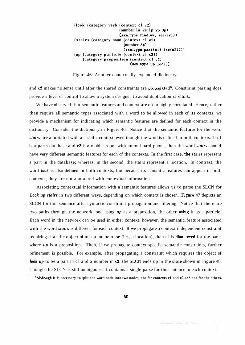
(look (category verb (context c l c2) (number l a 2s l p 2p 3p) (sem-type f ind-ev, see-ev) ) )
( s t a i r s (category noun (context c l c2) (number 3p) (aem-type part(c1) l o c ( c 2 ) ) ) )
(up (category par t i c l e (context c l c2) ) (category preposit ion (context c l c2)
(sem-type up-loc) 1)
Figure 46: Another contextually expanded dictionary.
and c2 makes no sense until after the shared constraints are propagated6. Constraint parsing does
provide a level of control to allow a system designer to avoid duplication of effolrt.
We have observed that semantic features and context are often highly correlated. Hence, rather
than require all semantic types associated with a word to be allowed in each of its contexts, we
provide a mechanism for indicating which semantic features are defined for each context in the
dictionary. Consider the dictionary in Figure 46. Notice that the semantic features for the word
stairs are annotated with a specific context, even though the word is defined in both contexts. If c l
is a parts database and c2 is a mobile robot with an on-board phone, then the word stairs should
have very different semantic features for each of the contexts. In the first case, ithe stairs represent
a part in the database; whereas, in the second, the stairs represent a location. In contrast, the
word look is also defined in both contexts, but because its semantic features can appear in both
contexts, they are not annotated with contextual information.
Associating contextual information with a semantic features allows us to parse the SLCN for
Look up stairs in two different ways, depending on which context is chosen. Figure 47 depicts an
SLCN for this sentence after syntactic constraint propagation and filtering. Notice that there are
two paths through the network, one using up as a preposition, the other usiilg it as a particle.
Each word in the network can be used in either context; however, the semantic. feature associated
with the word stairs is different for each context. If we propagate a context independent constraint
requiring that the object of an up-loc be a loc (i.e., a location), then c l is disalllowed for the parse
where up is a preposition. Then, if we propagate context specific semantic constraints, further
refinement is possible. For example, after propagating a constraint which requires the object of
look up to be a part in c l and a number in c2, the SLCN ends up in the state shown in Figure 48.
Though the SLCN is still ambiguous, it contains a single parse for the sentence in each context.
'Although it is necessary to split the word node into two nodes, one for contexts cl and c2 .and one for the others.

Figure 47: An SLCN after syntactic constraint propagation.
Figure 48: An SLCN after semantic and contextual constraint propagation.
In conclusion, we have described a system which is capable of utilizing a variety of knowledge
sources to select the most appropriate parse for a spoken sentence. These knowledge sources
include syntax, semantics, and contextual information. The parser uses a uiliform mechanism,
constraint propagation, t o apply these high-level knowledge sources t o prune a wsord graph provided
by the speech recognizer. Constraints for different knowledge sources can be dt?veloped somewhat
independently and used incrementally when parsing a sentence. Our constraint-based parser should
prove an important component for a spoken language interface t o several computer applications,
where each application defines its own context.
References
[I] J . Allen. Natuml Language Understanding. The Benjamin Cummings Pu'blishing Company,
Menlo Park, CA, 1987.
[2] J. Barwise and J. Perry. Situations and Attitudes. The MIT Press, Cambridge, MA, 1983.
[3] J. Bear and P. Price. Prosody, syntax, and parsing. In Pmeedings of the 28th annual ACL,
1990.
[4] P. Dey and B. R. Bryant. Lexical ambiguity in tree adjoining grammars. Information Pro-
cessing Letters, 34:65-69, 1990.
.[5] M. P. Harper. Ambiguous noun phrases in logical form. Computational Lin!guistics, 18(4):419-
465, 1992.
[6] M. P. Harper and R. A. Helzerman. PARSEC: A constraint-based parser for spoken language
parsing. Technical Report EE-93-28, Purdue University, School of Electrical Engineering, West
Lafayette, IN, 1993.
[7] M. P. Harper, L. H. Jamieson, C. B. Zoltowski, and R. A. Helzerman. Semantics and constraint
parsing of word graphs. In Proceedings of the International Conference on Acoustics, Speech,
and Signal Processing, volume 11, pages 63-66, April 1992.
[8] R. A. Helzerman. PARSEC: A framework for parallel natural language understanding. Master's
thesis, Purdue University, School of Electrical Engineering, West Lafayettt?, IN, 1993.
[9] R. A. Helzerman and M. P. Harper. Log time parsing on the MasPar MP-11. In Proceedings of
the Sizth International Conference on Pamllel Pmessing, August 1992.
[lo] R. A. Helzerman and M. P. Harper. An approach to multiply segmented corlstraint satisfaction
problems. In Proceedings of the National Conference on Artificial Intelligence, July 1994.
[ l l ] R. A. Helzerman and M. P. Harper. MUSE CSP: An extension to the co~lstraint satisfaction
problem. Technical Report EE-94-8, Purdue University, School of Electricil Engineering, West
Lafayette, IN, 1994.
[12] A. K. Joshi, L. S. Levy, and M. Takahashi. Tree adjunct grammars. Journal of Computer and
System Sciences, 10:136-163, 1975.
[13] S. R. Kosaraju. Speed of recognition of context-free languages by array automata. SIAM
Journal of Computing, 4 (3 ) :331-340, September 1975.
[14] V. Kumar. Algorithms for constraint-satisfaction problems: A survey. A I hTagazine, 13(1):32-
44, 1992.
[15] H. Maruyama. Constraint dependency grammar. Technical Report #RT0044, IBM, Tokyo,
Japan, 1990.
[16] H. Maruyama. Constraint dependency grammar and its weak generative c.apacity. Computer
Software, 1990.
[17] H. Maruyama. Structural disambiguation with constraint propagation. In The Proceedings of
the Annual Meeting of ACL, 1990.
[18] R. Mohr and T. Henderson. Arc and path consistency revisited. Artifici:al Intelligence, 28,
1986.
[19] U . Montanari. Networks of constraints: Fundamental properties and appllications t o picture
processing. Information Science, 1976.
[20] M. D. Moshier and W. C. Rounds. On the succinctness properties of unordered context-free
grammars. In Proceedings of the 25th Annual Meeting of the Association for Computational
Linguistics, 1987.
[21] M. A. Palis, S. Shende, and D. S. L. Wei. An optimal linear-time parallel parser for tree
adjoining languages. SIAM Journal of Computing, 19: 1-31,1990.
[22] W. Ruzzo. Tree-size bounded alternation. Journal of Computers and System Sciences, 21:218-
235,1980.
[23] R. Schwartz and Y-L. Chow. The N-best algorithm: An efficient and exact procedure for
finding the N most likely sentence hypotheses. In IEEE Int. Conf. Acoustics, Speech, and
Signal Processing, April 1990.
[24] K. Vijayashanker and A. K. Joshi. Some computational properties of tree adjoining grammars.
In Proceedings of the 24th Annual Meeting of the Association for Compui.ationa1 Linguistics,
1986.

[25] K. Vijayshanker, D.J. Weir, and A. K. Joshi. Characterizing structural descriptions produced
by various grammatical formalisms. In Proceedings of the 25th Annual Meeting of the Associ-
ation for Computational Linguistics, 1987.
[26] D. L. Waltz. Understanding line drawings of scenes with shadows. In P. H:. Winston, editor,
The Psychology of Computer Vision. McGraw Hill, New York, 1975.
[27] C. B. Zoltowski, M. P. Harper, L. H. Jamieson, and R. A. Helzerman. PARSEC: A constraint-
based framework for spoken language understanding. In Proceedings of the .hternational Con-
femnce on Spoken Language Understanding, October 1992.