managing material and financial flows in supply chains

Managing Material and Financial Flows in

Supply Chains

by

Wei Luo

Department of Business AdministrationDuke University

Date:Approved:

Kevin H. Shang, Supervisor

Fernando G. Bernstein

Li Chen

John R. Graham

Dissertation submitted in partial fulfillment of the requirements for the degree ofDoctor of Philosophy in the Department of Business Administration

in the Graduate School of Duke University2013

Abstract

Managing Material and Financial Flows in

Supply Chains

by

Wei Luo

Department of Business AdministrationDuke University

Date:Approved:

Kevin H. Shang, Supervisor

Fernando G. Bernstein

Li Chen

John R. Graham

An abstract of a dissertation submitted in partial fulfillment of the requirements forthe degree of Doctor of Philosophy in the Department of Business Administration

in the Graduate School of Duke University2013

Copyright © 2013 by Wei LuoAll rights reserved except the rights granted by the

Creative Commons Attribution-Noncommercial Licence

http://creativecommons.org/licenses/by-nc/3.0/us/

Abstract

This dissertation studies the integration of material and financial flows in supply

chains, with the goal of examining the impact of cash flows on the individual firm’s

decision making and the overall supply chain efficiency. We develop analytical models

to provide effective policy recommendations and derive managerial insights.

We first consider a credit-constrained firm that orders inventory to satisfy stochas-

tic demand in a finite horizon. The firm provides trade credit to the customer and

receives it from the supplier. A default penalty is incurred on the unfulfilled payment

to the supplier. We utilize an accounting concept of working capital to obtain optimal

and near-optimal inventory policies. The model enables us to suggest an acceptable

purchasing price offered in the supplier’s trade credit contract, and to demonstrate

how liquidity provision can mitigate the bullwhip effect.

We then study a joint inventory and cash management problem for a multi-

divisional supply chain. We consider different levels of cash concentration: cash

pooling and transfer pricing. We develop the optimal joint inventory replenishment

and cash retention policy for the cash pooling model, and construct cost lower bounds

for the transfer pricing model. The comparison between these two models shows the

value of cash pooling, although a big portion of this benefit may be recovered through

optimal transfer pricing schemes.

Finally, we build a supply chain model to investigate the material flow variability

without cash constraint. Our analytical results provide conditions under which the

material bullwhip effect exists. These results can be extended to explain the similar

effect when financial flows are involved.

iv

In sum, this dissertation demonstrates the importance of working capital and

financial integration in supply chain management.

v

To My Family

vi

Contents

Abstract iv

List of Tables x

List of Figures xi

List of Abbreviations and Symbols xii

Acknowledgements xix

1 Introduction 1

2 Inventory Systems with Trade Credit 4

2.1 Introduction . . . . . . . . . . . . . . . . . . . . . . . . . . . . . . . . 5

2.2 Literature Review . . . . . . . . . . . . . . . . . . . . . . . . . . . . . 9

2.3 The Model . . . . . . . . . . . . . . . . . . . . . . . . . . . . . . . . . 12

2.4 Balanced Credit Periods . . . . . . . . . . . . . . . . . . . . . . . . . 17

2.4.1 State Space Reduction . . . . . . . . . . . . . . . . . . . . . . 17

2.4.2 The Optimal Policy . . . . . . . . . . . . . . . . . . . . . . . . 19

2.5 Longer Payment Period (m ą n) . . . . . . . . . . . . . . . . . . . . . 23

2.5.1 Linear Approximation . . . . . . . . . . . . . . . . . . . . . . 24

2.5.2 Lower Bound Solutions . . . . . . . . . . . . . . . . . . . . . . 26

2.5.3 Heuristics . . . . . . . . . . . . . . . . . . . . . . . . . . . . . 31

2.6 Longer Collection Period (m ă n) . . . . . . . . . . . . . . . . . . . . 32

2.7 Numerical Study . . . . . . . . . . . . . . . . . . . . . . . . . . . . . 33

2.7.1 Effectiveness of the Heuristics . . . . . . . . . . . . . . . . . . 33

vii

2.7.2 Impact of Payment Periods . . . . . . . . . . . . . . . . . . . 36

2.7.3 Bullwhip Effect . . . . . . . . . . . . . . . . . . . . . . . . . . 38

2.8 Conclusion . . . . . . . . . . . . . . . . . . . . . . . . . . . . . . . . . 40

3 Joint Inventory and Cash Management 41

3.1 Introduction . . . . . . . . . . . . . . . . . . . . . . . . . . . . . . . . 42

3.2 Literature Review . . . . . . . . . . . . . . . . . . . . . . . . . . . . . 48

3.3 Cash Pooling System . . . . . . . . . . . . . . . . . . . . . . . . . . . 51

3.3.1 Echelon Formulation . . . . . . . . . . . . . . . . . . . . . . . 55

3.3.2 The Optimal Policy . . . . . . . . . . . . . . . . . . . . . . . . 57

3.4 Transfer Pricing System . . . . . . . . . . . . . . . . . . . . . . . . . 61

3.4.1 Echelon Formulation . . . . . . . . . . . . . . . . . . . . . . . 63

3.4.2 Lower Bounds . . . . . . . . . . . . . . . . . . . . . . . . . . . 64

3.4.3 Optimal Transfer Pricing Model . . . . . . . . . . . . . . . . . 68

3.5 Numerical Study . . . . . . . . . . . . . . . . . . . . . . . . . . . . . 69

3.5.1 Value of Cash Pooling . . . . . . . . . . . . . . . . . . . . . . 70

3.5.2 Optimal Transfer Pricing . . . . . . . . . . . . . . . . . . . . . 73

3.5.3 Bullwhip Effect . . . . . . . . . . . . . . . . . . . . . . . . . . 75

3.6 Concluding Remarks . . . . . . . . . . . . . . . . . . . . . . . . . . . 76

4 Material Flow Variability 78

4.1 Introduction . . . . . . . . . . . . . . . . . . . . . . . . . . . . . . . . 78

4.2 Main Results . . . . . . . . . . . . . . . . . . . . . . . . . . . . . . . 78

A Proof of Results 85

A.1 Proof of Results in Chapter 2 . . . . . . . . . . . . . . . . . . . . . . 85



Bibliography 101

viii

Biography 107

ix

List of Tables

2.1 Events and accounting variables associated with the cash conversioncycle . . . . . . . . . . . . . . . . . . . . . . . . . . . . . . . . . . . . 14

2.2 Demand mean and responsive working capital requirement . . . . . . 35

3.1 Value of cash pooling - i.i.d. demand (left) and increasing demand (right) 71

x

List of Figures

2.1 The cash conversion cycle . . . . . . . . . . . . . . . . . . . . . . . . 13

2.2 The base model with material and cash flows . . . . . . . . . . . . . . 14

2.3 The optimal solution of the transformed λ-model . . . . . . . . . . . 21

2.4 Linear approximations and optimal control policies . . . . . . . . . . 26

2.5 The optimal solution of the three-piece lower bound . . . . . . . . . . 30

2.6 Impact of system parameters on the cost reduction through paymentperiod extension . . . . . . . . . . . . . . . . . . . . . . . . . . . . . 37

2.7 Customer payment default and bullwhip effect . . . . . . . . . . . . 39

3.1 The two-stage cash pooling model with material and cash flows . . . 52

3.2 The three-stage transformed cash pooling system . . . . . . . . . . . 56

3.3 Induced penalty functions of the cash pooling model . . . . . . . . . . 60

3.4 Transformation of the transfer pricing model . . . . . . . . . . . . . . 62

3.5 Decomposition of the transfer pricing system . . . . . . . . . . . . . . 65

3.6 The transformed optimal pricing model . . . . . . . . . . . . . . . . . 69

3.7 Value of cash pooling . . . . . . . . . . . . . . . . . . . . . . . . . . . 72

3.8 Product life cycle demand . . . . . . . . . . . . . . . . . . . . . . . . 74

3.9 Optimal transfer price under product life cycle demand . . . . . . . . 74

4.1 The two-stage supply chain model with material and information flows 79

4.2 Variance of shipment varpM1,tq vs. base-stock s2 under Up0, 12q . . . 82

4.3 Bullwhip ratio varpM2,tq{varpM1,tq vs. base-stock s2 under Up0, 12q . 82

4.4 varpM1,tq and varpM0,t´1q as a function of base-stock s2 under Up0, 12q 84

xi

List of Abbreviations and Symbols

Symbols

Notations for Chapter 2

a1 left-control threshold in the pd, a, Sq policy.

a2 right-control threshold in the pd, a, Sq policy.

A1 left-adjustment in the three-piece linear approximation.

A2 right-adjustment in the three-piece linear approximation.

b backorder penalty cost rate.

B band in which inventory does not exceed base-stock level.

c unit procurement cost.

C2 cost of the pd, a, Sq heuristic.

C3 cost of the three-piece lower bound.

C3 cost of the pd, Sq heuristic.

CL cost of lower bound under negative demand shocks.

CU cost of heuristic under negative demand shocks.

d default threshold.

d expected default threshold.

D random customer demand.

e column vector of ones.

E expectation.

f probability density function (p.d.f.) of D.

xii

F cumulative distribution function (c.d.f.) of D.

F complementary cumulative distribution function (c.c.d.f.) of D.

F loss function of D.

g default-free single-period cost function.

G single-period cost function.

h inventory holding cost rate.

H single-period holding and backorder cost function.

L default penalty linear function.

m payment period.

M default penalty cost function.

M´ two-piece linear approximation of M .

M three-piece linear approximation of M .

n collection period.

p default penalty rate (per unit inventory).

p expected default penalty rate (per unit inventory).

p1 default penalty rate (per dollar).

P accounts payable.

P vector of accounts payable.

Pr probability.

r unit revenue retained for operations (working capital require-ment).

R accounts receivable.

R vector of accounts receivable.

R doubtful receivable.

S default-free base-stock level.

t time variable.

T time horizon.

xiii

u default quantity.

v unconstrained myopic minimization function.

Vt minimum expected cost function over t to T ` 1.

w working capital level (in inventory unit).

w expected working capital level.

w1 net cash level.

W decoupled cost-to-go function of working capital.

x net inventory level.

y inventory position.

z order quantity.

α discount factor.

Γ linear function in the three-piece approximation.

δ estimated proportion of collectible receivable.

ε random variable representing the payment default uncertainty.

θ r{c´ 1.

λ minimum of the payment period and the collection period.

µ mean of demand D.

µ mean of ε.

ρ r{c.

σ standard deviation of demand D.

σ standard deviation of ε.

˚ optimal.

ˆ pre-transformation function.

¯ three-piece lower bound function.

ďst stochastically increasing.

^ minimum.

_ maximum.

xiv


For stage i “ 1, 2, echelon j “ 1, 2, 3, 4, and subsystem k “ 1, 2

b backorder penalty cost rate.

B constant in the flow conservation equation.

c unit procurement cost from the outside vendor.

CL cost of the integrated lower bound.

CO cost of the optimal pricing model.

CR cost of the constraint relaxation bound.

CS cost of the sample path bound.

C˚ optimal cost of the cash pooling model.

dpωq demand realization given sample path ω.


E expectation.

fj,t expected optimal cost for echelon j over t to T ` 1.

gj single-period cost function for echelon j (without transactioncost).

G single-period cost function.

Gk single-period cost function for subsystem k.

hi inventory holding cost rate of stage i.

Hj single-period holding and backorder cost function of echelon j.

Hk1 single-period holding and backorder cost function of echelon 1 for

subsystem k.

Jt expected cost function over t to T ` 1.

K upper-limit of asset that can be liquidated to assist operations.

l˚ lower threshold in the cash retention policy.

L lower threshold linear function.

p1 unit selling price to the end customer.

xv

p2 unit transfer price.

r working capital position in the cash pooling model.

r1 working capital position of stage 1 in the transfer pricing model.

rf risk-free rate.

R return rate for external investment.

S constraint set.

Sd constraint set under deterministic demand.

t time variable.

T time horizon.

u˚ upper threshold in the cash retention policy.

U upper threshold linear function.

v amount of cash transferred into the operating account.

Vt minimum expected cost function over t to T ` 1.

V kt minimum expected cost function over t to T `1 for subsystem k.

V dt minimum expected cost function over t to T ` 1 for subsystem

2, given demand sample path.

w net working capital level in the cash pooling model.

wi echelon working capital level of stage i in the transfer pricingmodel.

w1 cash balance in the pooled account.

w1i cash balance in stage i’s account.

xi echelon i net inventory level.

x11 net inventory level at stage 1.

x12 on-hand inventory level at stage 2.

yj inventory position for echelon j.

zi order quantity for stage i.

α discount factor.

xvi

βi unit transaction cost on cash transferred into the operating ac-count.

βo unit transaction cost on cash transferred out of the operatingaccount.

Γ2 induced penalty cost from echelon 1 to echelon 2.

Γ3 induced penalty cost from echelon 2 to echelon 3.

η cash holding cost rate of the pooled account.

ηi cash holding cost rate of stage i.

θ p1{c´ 1.

Λ2 induced penalty cost from echelon 3 to echelon 2.

Λ3 self-induced penalty cost at echelon 3.

ρ p2{c.

ω demand sample path.

˚ optimal.

1 local; e.g.,

η1 “ local cash holding cost,

η “ echelon cash holding cost.

ˆ pre-transformation function.

^ minimum.

_ maximum.


j “ 1, 2

Bj local backorders of stage j.


E expectation.

ILj local net inventory level of stage j.

Mj shipment released to stage j from its upstream supplier.

xvii

M0 realized sales to the end customer.

Oj order quantity from stage j to its upstream supplier.

sj local base-stock level of stage j.

t time variable.

Up0, dq uniform distribution with support r0, ds.

var variance.

τ cycle length.

Abbreviations

CCC cash conversion cycle.

A/P accounts payable.

A/R accounts receivable.

LC letter of credit.

CP cash pooling.

TP transfer pricing.

OP optimal pricing.

CR constraint relaxation.

SP sample path.

xviii

Acknowledgements

My foremost gratitude goes to my advisor, Prof. Kevin Shang, for his guidance and

support along the course of my graduate study. He patiently provided the vision,

encouragement and advice necessary for me to conduct research and complete this

dissertation. I also extend my thanks to other members of my dissertation commit-

tee, Professors Fernando Bernstein, Li Chen, and John Graham, for their inspiring

suggestions and extensive time commitment. I am grateful to the Ph.D. program at

the Fuqua School of Business for fellowship funding, and to Prof. Kevin Shang for

his research support.

My deep appreciation also goes to other faculty in the Operations Management

area, Professors Jeannette Song, Gurhan Kok, Paul Zipkin, Otis Jennings, and Pranab

Majumder, as well as faculty from other areas at Duke and UNC Chapel Hill, espe-

cially Professors Peng Sun, David Brown, Jennifer Francis, Shane Dikolli, Gabor

Pataki, and Serhan Ziya, for their help in both research and coursework.

Papers contained in this dissertation have been presented at various conferences,

invited seminars and workshops: INFORMS Annual Meeting 2011, 2012, MSOM

iFORM SIG Conference 2012, POMS Annual Conference 2012, 2013, Duke-UNC

Workshop 2012, Singapore Management University, IESE Business School, University

of California, Irvine, Dartmouth College, Chinese University of Hong Kong, City Uni-

versity of Hong Kong, Singapore University of Technology and Design, and Shanghai

Jiao Tong University. I am grateful to the participants for their constructive feedback.

Finally, I would like to thank my family who constantly supported me throughout

my life. Without their help, I certainly could not have pursued an academic career.

xix

1

Introduction

With the worldwide economic crisis rendering bank financing increasingly difficult

to secure, coordination between material and financial flows has taken on added

importance. Great opportunities and challenges lie ahead in managing the financial

flows in supply chains. More specifically, in a logistics-integrated supply chain, the

trading partners jointly determine inventory replenishment according to the demand

information without considering each partner’s financial condition. This makes sense

if the financial market is perfect (Modigliani and Miller 1958). However, when there

are market frictions, the supply chain partners have to jointly maintain a healthy

financial ecosystem in order to drive operational efficiencies.

Nevertheless, the literature on the integration of material and financial flows is

relatively sparse, even though these two flows are closely related and affect each other.

This dissertation constructs a modeling framework to explicitly incorporate financial

flows into the inventory system of a single firm, and a multi-divisional supply chain.

It seeks to address the following research questions. From a single firm’s perspective,

what is the impact of upstream and downstream payment terms on firm’s optimal

replenishment decisions? What is the right cash conversion cycle for a firm that

faces various demand patterns and working capital requirements? From a supply

1

chain’s perspective, what is the value of cash pooling? How much of this value can be

recovered through advanced internal transfer pricing scheme? And how does financial

flow affect the material bullwhip effect in the supply chain? The answers to these

research questions can be found in the following three chapters.

Chapter 2 considers a single firm that orders inventory periodically to satisfy

random customer demand in a finite horizon. The firm provides trade credit to its

customer while receiving trade credit from its supplier. The trade credit is in the

form of a one-part contract, i.e., the payment is due within a specific period of time

following the invoice. A default penalty cost is incurred on the unfulfilled payment

to the supplier. The objective is to obtain an inventory policy that minimizes the

total inventory related and default penalty cost. Utilizing an accounting concept of

work capital (which incorporates cash, inventory, accounts receivable and accounts

payable), we prove that a myopic policy is optimal when the sales collection period is

longer than or equal to the purchases payment period. The myopic policy has a simple

structure – an order is placed to achieve a target base-stock level that depends on the

firm’s working capital. When the payment period is longer than the collection period,

we derive a lower bound to the optimal cost and propose an effective heuristic that has

a generalized form of the above structured policy. These policies resemble practical

working capital management under which firms decide inventory policies according to

their working capital status. The policy parameters have a closed-form expression,

which shows the impact of demand variability on the inventory decision and the

tradeoff between cost parameters. The model enables us to suggest an acceptable



Chapter 3 develops a centralized supply chain model that aims to assess the value

of cash pooling. The supply chain is owned by a single corporation with two divisions,

where the downstream division (headquarter), facing random customer demand, re-

plenishes materials from the upstream one. The downstream division receives cash

2

payments from customers and determines a system-wide inventory replenishment and

cash retention policy. We consider two cash management systems that represent dif-

ferent levels of cash concentration. For cash pooling, the supply chain adopts a

financial services platform which allows the headquarter to create a corporate master

account that aggregates the divisions’ cash. For transfer pricing, on the other hand,

each division owns its cash and pays for the ordered material according to a fixed

price. Comparing both systems yields the value of adopting such financial services.

We prove that the optimal policy for the cash pooling model has a surprisingly sim-

ple structure – both divisions implement a base-stock policy for material control; the

headquarter monitors the corporate working capital and implements a two-threshold

policy for cash retention. Solving the transfer pricing model is more involved. We

derive a lower bound on the optimal cost by connecting the model to an assembly

system. Our results show that the value of cash pooling can be very significant when

demand is increasing (stationary) and the markup for the upstream division is small

(high). Nevertheless, a big portion of the pooling benefit may be recovered if the

headquarter can decide the optimal transfer price and the lead time is short.

Chapter 4 focuses on the material bullwhip effect in supply chains, a phenomenon

that the variability of shipment is amplified when moving upstream the supply chain.

Economists have observed this phenomenon in empirical studies. However, this ob-

servation appears to be counter-intuitive as they would expect the opposite - the

“production smoothing” effect (smaller shipment variability at the upstream stage).

We provide an analytical model to show that it is possible to observe both bullwhip

and variability dampening in supply chains. These results can be extended to explain

the similar effect when inventory replenishment is subject to the cash constraint,

hence providing analytical support for the findings in Chapter 2 and Chapter 3.

The Appendix contains all the proofs.

3

2

Inventory Systems with Trade Credit

This chapter considers a firm that orders inventory periodically to satisfy random

customer demand in a finite horizon. The firm provides trade credit to its customer

while receiving trade credit from its supplier. The trade credit is in the form of a one-

part contract, i.e., the payment is due within a specific period of time following the

invoice. A default penalty cost is incurred on the unfulfilled payment to the supplier.

The objective is to obtain an inventory policy that minimizes the total inventory

related and default penalty cost. Utilizing an accounting concept of work capital

(which incorporates cash, inventory, accounts receivable and accounts payable), we

prove that a myopic policy is optimal when the sales collection period is longer than

or equal to the purchases payment period. The myopic policy has a simple structure

– an order is placed to achieve a target base-stock level that depends on the firm’s

working capital. When the payment period is longer than the collection period, we

derive a lower bound to the optimal cost and propose an effective heuristic that has

a generalized form of the above structured policy. These policies resemble practical

working capital management under which firms decide inventory policies according to

their working capital status. The policy parameters have a closed-form expression,

which shows the impact of demand variability on the inventory decision and the

4

tradeoff between cost parameters. The model enables us to suggest an acceptable



2.1 Introduction

Trade credit is widely used for business transactions in supply chains, and is the single

most important source of external finance for firms (Petersen and Rajan, 1997). It

appears on every balance sheet and accounts for about one half of the short-term

debt in two samples of UK and US firms (Cunat, 2007). In the finance literature,

there have been various theories to explain the existence of trade credit despite its

high cost. Our paper takes trade credit as a premise and aims to investigate the

impact of trade credit on a firm’s inventory policy and operating cost. We consider

a firm that orders inventory periodically to satisfy stochastic customer demand in a

finite horizon. The firm grants trade credit to its customer while obtaining it from

its supplier. (We do not consider bank financing in the model.) The trade credit

we consider is a one-part contract, that is, the payment is due within a certain time

period after the invoice is issued1. Thus, the firm pays for the ordered inventory after

a deferral period following the delivery of goods, and receives sales revenue after a

collection period following the demand. In the 1998 NSSBF survey, however, 46%

of the firms declared that they had made some payments to their suppliers after

the due date. These delayed payments often do not carry an explicit penalty for

the customers (Cunat, 2007). Nevertheless, payment default will hurt a firm’s credit

record, making it hard to finance in the future2. In light of this intangible cost, we

introduce a default penalty cost incurred upon the unfulfilled payment to the firm’s

supplier. The objective is to obtain an inventory ordering policy that minimizes the

1 According to the 1998 National Survey of Small Business Finance (NSSBF), 49% of the tradecredit contracts are one-part.

2 For example, Dun and Bradstreet keeps credit records and provides credit reports of small busi-nesses.

5

total discounted system cost, which consists of the inventory purchasing cost, holding

and backorder costs, as well as the default penalty cost.

Our research question is related to a broader issue of working capital management.

Working capital refers to the difference between current assets and current liabilities

(assets and liabilities with maturities of less than one year). On the balance sheet,

current assets include cash, short-term investments, accounts receivable (A/R), and

inventory, while current liabilities include accounts payable (A/P) and short-term

loans. In our model, the deferred payment is recorded as A/P and the delayed

sales collection as A/R. The goal of working capital management is to increase the

profitability of a firm and to ensure that it has sufficient liquidity to meet short-term

operations so to continue in business (Pass and Pike, 1984). Profitability and liquidity

are conflicting goals as investments in current assets usually lead to a smaller return.

Thus, a firm needs to decide a working capital policy, which budgets how much

revenue received to be invested in working capital. In general, a firm can adopt three

types of working capital strategies: aggressive, moderate, and conservative (Gallagher

and Andrew, 2007). (With aggressive strategy firms choose to operate with low cash,

inventory, and trade receivables.) In this paper, we assume a given working capital

strategy and aim to study the optimal inventory policy when trade credits are present.

Most inventory models in the literature do not explicitly consider the interrela-

tionship between the inventory decision and the accounts payable/receivable because

traditionally the former is a function of an operations manager and the latter a

treasurer or controller. We find it important to study this interrelationship for the

following reasons. First, today’s inventory order decision will directly affect the future

cash payment. If a firm orders too much, it is not only to incur a higher purchase

cost and possibly inventory holding cost, but also to increase the chance of payment

default as the future cash balance may not be enough to pay off the current inven-

tory order due to demand/sales uncertainty. On the other hand, if a firm orders too

little, it is more likely to incur a higher backorder cost. Thus, there is a clear tradeoff

6

between these system costs when making an inventory decision. Second, a firm often

wishes to extend the payment period and shorten the collection period so that its cash

conversion cycle (cash collection periods + on-hand inventory in periods - inventory

payment periods) can be reduced. However, extending the payment period may lead

to an increase of the unit wholesale price, and thus may not be ideal for the firm.

Therefore, it would be useful to provide a decision support tool that characterizes the

tradeoff between a longer payment period and a higher purchase cost.

We formulate the inventory system with trade credit into a multi-state dynamic

program that keeps track of inventory level, cash balance, as well as different ages of

accounts payable and accounts receivable within the payment and collection periods,

respectively. This dynamic program is hard to solve because the state space is high-

dimensional. We borrow a concept in accounting called working capital (= cash +

inventory + accounts receivable - accounts payable) to redefine the state and simplify

the original dynamic program. We consider three cases regarding the different lengths

of payment and collection periods. When the payment period is equal to or less than

the collection period, we prove that a myopic policy is optimal when the demand is

non-decreasing. The optimal policy is operated under two control parameters pd, Sq,

d ď S: the firm reviews its inventory-equivalent working capital level (i.e., working

capital divided by the unit purchase cost) and inventory position at the beginning

of each period; if the working capital is lower (higher) than d(S), the firm places

an order to bring its inventory position up to d(S); if the working capital level is

between d and S, the firm orders up to the working capital level. When the payment

period is longer than the collection period, the firm’s future payment depends on the

future cash inflow, which in turn depends on the random demand. Consequently, it

is difficult to characterize the optimal policy. Nevertheless, we develop a lower bound

to the optimal cost and propose an effective heuristic. The heuristic policy, referred

to as the pd, a, Sq policy, is operated under five control parameters and can be viewed

as a generalization of the pd, Sq policy. In a numerical study, we show that the heuris-

7

tic is near optimal. The optimal and heuristic policy parameters have a closed-form

expression which allows us to investigate the impact of demand variability on the

inventory decision as well as the tradeoffs between inventory holding cost, backorder

cost, and payment default cost. Finally, we also test our optimal and heuristic policies

under different non-stationary demand forms, and the performance remains satisfac-

tory. Thus, the suggested policies can comfortably be applied to systems with general

demand patterns. Notice that the heuristics resemble practical working capital man-

agement under which firms determine the inventory policy according to the working

capital level. Consequently, we can use them to gain insights.

We summarize the main contributions and key insights obtained from this study.

First, managers are hindered from integrating accounts payable/receivable into the

inventory policy due to the typical organizational structure of the firm. These two

functions need to be aligned in order to improve the firm’s profit. Our model cap-

tures the dynamics between inventory decision as well as accounts payable/receivable

resulted from trade credit terms and provide a simple and implementable inventory

policy. Second, the optimal policy suggests that a firm should consider working cap-

ital when making inventory decisions. This result naturally connects operations to

accounting. Also, the closed-form expression for the optimal policy suggests that a

firm would possibly choose to default on the payment to its supplier if its current work-

ing capital level is low and the backorder penalty is higher than the default penalty.

This result echoes the NSSBF survey that 46% of firms experience payment defaults.

Third, we provide a decision support tool in trade credit contract negotiation by quan-

tifying the impact of payment periods on the firm’s total operating cost. We find that

increasing demand and high backorder cost justify the usage of trade credit despite

its high cost. In addition, our numerical study shows that firms with a shorter cash

conversion cycle have more incentive to extend credit periods with suppliers, which

predicts a positive correlation between the firm’s upstream and downstream credit

periods. Finally, we show that customer payment default drives the bullwhip effect.

8

The bullwhip ratio increases with the downstream default volatility and the upstream

default penalty cost. This suggests that the supplier could effectively mitigate the

bullwhip effect through liquidity provision.

2.2 Literature Review

Our paper is related to inventory systems with trade credit contracts. This literature

can be categorized based on whether a single- or multi-period problem is considered.

For the single-period model, Zhou and Groenevelt (2008) consider the impact of

financial collaboration in a third-party supply chain. They find that the total supply

chain profit with bank financing is slightly higher than that with open account (trade

credit) financing. Yang and Birge (2012) study how different priority rules of order

repayment influence trade credit usage.

As for the multi-period model, this literature can be further categorized based on

how trade credits are modeled. One category is to characterize the impact of trade

credit on the inventory holding cost. Beranek (1967) uses a lot-size model to illustrate

how a firm’s inventory holding cost should be adjusted according to the firm’s actual

financial arrangements. Maddah et al. (2004) investigate the effect of permissible

delay in payments on ordering policies in a periodic review ps, Sq inventory model

with stochastic demand. They develop heuristic approaches to approximate inventory

control parameters. Gupta and Wang (2009) consider a stochastic inventory system

where trade credit term is modeled as a non-decreasing holding cost rate according

to an item’s shelf age. Under the assumption that the full payment is made when the

item is sold, they prove that a base-stock policy is optimal. Huh et al. (2010) and

Federgruen and Wang (2010) generalize the results of Gupta and Wang. Song and

Tong (2012) consider an inventory system where a base-stock policy is implemented.

They investigate how the holding cost rate is affected by the different payment and

collection periods.

Another category, which is more related to our model, is to explicitly characterize

9

cash flow dynamics resulted from the trade credit terms. Haley and Higgins (1973)

expand Beranek’s model and consider a problem of jointly optimizing inventory deci-

sion and payment times when demand is deterministic and inventory is financed with

trade credit. Schiff and Lieber (1974) consider a problem of optimizing inventory and

trade credit policy for a firm where the demand is deterministic but depends on the

credit term and inventory level. Bendavid et al. (2012) study a self-financing firm

whose replenishment decisions are constrained by the working capital requirement.

Their model is similar to ours in the sense that they also consider how inventory

replenishment is affected by the payment and the collection periods. However, their

model considers i.i.d demand and implements a base-stock policy with inventory or-

dering subject to a hard constraint - the working capital requirement. Thus, no

defaults are allowed. They characterize the dynamics of system variables and obtain

the optimal base-stock level via a simulation approach.

There has been an emerging research stream that aims to jointly model financial

and operational decisions without explicitly considering the trade credit. Xu and

Birge (2004) analyze the interactions between a firm’s production and financing deci-

sions as a tradeoff between the tax benefits of debt and financial distress costs. Li et al.

(2013) study a dynamic model in which inventory and financial decisions are made

simultaneously in order to maximize the expected present value of dividends net of

capital subscriptions. Xu and Birge (2006) propose an integrated corporate planning

model, which extends the forecasting-based discount dividend pricing method into an

optimization-based valuation framework to make production and financial decisions

simultaneously for a firm facing market uncertainty. Chao et al. (2008) consider a

self-financed retailer who replenishes inventory in a finite horizon. Luo and Shang

(2012) integrates material flow and cash flow in a supply chain. They characterize

the optimal joint policy and investigate the value of payment flexibility. Tanrisever

et al. (2012) explore the tradeoff between investment in process development and

reservation of cash in order to avoid bankruptcy for a start-up firm. They provide

10

managerial insights by characterizing how to create operational hedges against the

bankruptcy risk. Other noteworthy examples include Babich and Sobel (2004), Buza-

cott and Zhang (2004), Ding et al. (2007), Dada and Hu (2008), Kouvelis and Zhao

(2009), Caldentey and Chen (2010). The research questions in these papers are quite

different from ours.

The motivation and the assumption of our model are related to the following

empirical finance literature. Petersen and Rajan (1997) find that there is a greater

extension of credit by firms with negative income and negative sales growth. They

suggest that trade credit can be used as a signal of financial health of a firm. Wilson

and Summers (2002) provide reasons why suppliers still maintain business relation-

ships with retailers who default on their payments. This finding also supports our

payment default setup in a finite horizon model. Cunat (2007) provides an empirical

evidence that suppliers serve a role as liquidity providers insuring against liquidity

shocks that could endanger the survival of their customer relationships. Thus, the

high cost of trade credit can be interpreted as the insurance and default premium.

The paper provides an empirical support of the default penalty assumed in our model.

It also suggests that there is a big portion of firms that use one-part trade credit con-

tracts. Boissay and Gropp (2007) investigate liquidity shocks for small-sized French

firms. They find that the payment default in a supply chain stops when it reaches

firms that are large and have access to financial markets. Guedes and Mateus (2009)

examine the trade credit linkages on the propagation of liquidity shocks in supply

chains. It is a common practice that firms often provide trade credit to its customer

while receiving trade credit from its supplier. In a similar spirit, we also study the

relationship between trade credit and materials bullwhip effect in our model.

Finally, our model is related to two streams of inventory problems. The on-hand

cash in our model resembles a capacity constraint on inventory ordering. However,

we allow payment defaults (i.e., order more than the on-hand cash level) and the cash

balance is endogenously determined by the inventory decision. We refer the reader

11

to Tayur (1997) for a review and Levi et al. (2008) for recent developments. The

other stream is inventory systems with advance demand information. The incoming

and outgoing cash flows in accounts payable and receivable can be viewed as advance

cash flow information. For the research of advanced demand models, see Ozer and

Wei (2004) and references therein.

The rest of this chapter is organized as follows. §2.3 describes the model and for-

mulates the corresponding dynamic program. §2.4 focuses on the model with balanced

payment and collection periods and proves the optimal policy. §2.5 (§2.6) considers

the model with longer payment (collection) periods. §3.5 examines the effectiveness

of the heuristics, and discusses the qualitative insights through a numerical study.

§3.6 concludes. Proofs are provided in Appendix A.1. Throughout this chapter, we

define x` “ maxpx, 0q, x´ “ ´minpx, 0q, a_ b “ maxpa, bq, and a^ b “ minpa, bq.

2.3 The Model

We consider a finite-horizon, periodic-review inventory system where a firm orders

from its supplier and sells to its customer. Trade credit is employed for transactions

at both upstream and downstream and is in the form of a one-part contract, that is,

the firm pays its supplier after a payment period following the delivery of goods, and

receives cash from its customer after a collection period following the demand. In

accounting, the inventory payment period (sales collection period) is also referred to

as the payables (receivables) conversion period or days purchases (sales) outstanding.

The payment and collection periods jointly affect the cash conversion cycle (CCC).

Figure 2.1 illustrates the referenced times of four events associated with buying and

selling a discrete batch of inventories: R, inventory order received; S, inventory sold;

P, cash paid to the supplier, and C, cash collected from the customer. The CCC

has three components: the payment period represented by the time interval between

R and P; the inventory conversion period (or days in inventory) represented by the

time interval between R and S; the collection period represented by the time interval

12

between S and C. In practice, CCC is calculated as follows:

CCC “ Inventory conversion period` Collection period´ Payment period.

Transactions based on the trade credit will affect a firm’s accounts payable (A/P)

and accounts receivable (A/R). Table 2.1 lists the four events and the corresponding

changes in inventory and cash flow, as well as accounts payable and receivable.

Figure 2.1: The cash conversion cycle

We now formalize the above description into our model. Since the focus is on

cash and inventory dynamics under trade credit, for simplicity and without loss of

generality, we assume that lead time is zero. Let m be the payment period and n

be the collection period. The sequence of events is as follows: At the beginning of

period t, (1) inventory order decision is made; (2) shipment arrives; (3) payment due

in this period (corresponding to the inventory ordered in period t´m) is made to the

supplier; (4) default penalty is incurred in case of insufficient payment; (5) customer

payment due in this period (corresponding to the sales in period t ´ n) is collected.

During the period, demand is realized. At the end of the period, all inventory related

costs and default penalty cost are calculated. The objective is to minimize the firm’s

total discounted cost over the entire horizon of T periods.

Customer demand in period t is modeled as a nonnegative random variableDt with

probability density function (p.d.f.) ft, cumulative distribution function (c.d.f.) Ft,

mean µt and variance σ2t . The demand is independent from period to period but the

13

Table 2.1: Events and accounting variables associated with the cash conversion cycle

Label Transaction Inventory/Cash flow AccountingR Receiving X units of inventory Inventory Ò X A/P Ò $XS Selling Y units of inventory Inventory Ó Y A/R Ò $YP Paying $X to the supplier Cash Ó $X A/P Ó $XC Collecting $Y from the customer Cash Ò $Y A/R Ó $Y

distribution could be non-stationary. We assume that the unsatisfied demand is fully

backlogged. Figure 2.2 takes a snapshot of the system in period t with the material

and cash flows in solid and dashed arrows, respectively. We count the time forward.

As shown, Ptí and Rt´j denote the accounts payable and accounts receivable made

in period t ´ i and t ´ j, respectively, for i “ 0, 1, ...,m and j “ 0, 1, ..., n. So Pt´m

and Rtń are the most aged A/P and A/R, respectively.

Figure 2.2: The base model with material and cash flows

Let us now define the state and decision variables at the beginning of period t:

zt “ order quantity made in Event (1);

xt “ net inventory level before Event (2);

w1t “ net cash level before Event (3);

Pt “ pPt´m, ..., Pt´1q: m-dimensional vector of accounts payable;

Rt “ pRtń, ..., Rt´1q: n-dimensional vector of accounts receivable.

Denote Pit as the vector consisting of the first i elements of Pt, and Pí

t as vector

Pt without the first i elements. Let r be the unit revenue retained for operations3

3 Firms usually determine an operations budget as a percentage of sales revenue during an inte-

14

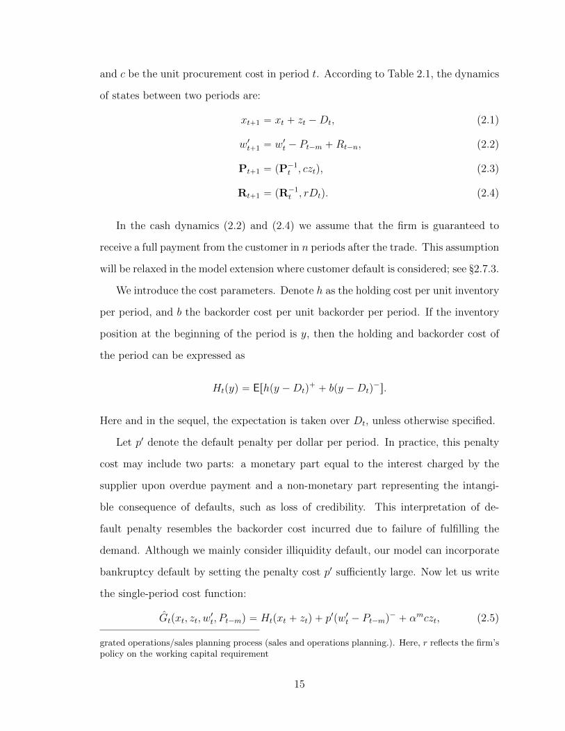
and c be the unit procurement cost in period t. According to Table 2.1, the dynamics

of states between two periods are:

xt`1 “ xt ` zt ´Dt, (2.1)

w1t`1 “ w1t ´ Pt´m `Rt´n, (2.2)

Pt`1 “ pP´1t , cztq, (2.3)

Rt`1 “ pR´1t , rDtq. (2.4)

In the cash dynamics (2.2) and (2.4) we assume that the firm is guaranteed to

receive a full payment from the customer in n periods after the trade. This assumption

will be relaxed in the model extension where customer default is considered; see §2.7.3.

We introduce the cost parameters. Denote h as the holding cost per unit inventory

per period, and b the backorder cost per unit backorder per period. If the inventory

position at the beginning of the period is y, then the holding and backorder cost of

the period can be expressed as

Htpyq “ Erhpy ´Dtq`` bpy ´Dtq

´s.

Here and in the sequel, the expectation is taken over Dt, unless otherwise specified.

Let p1 denote the default penalty per dollar per period. In practice, this penalty

cost may include two parts: a monetary part equal to the interest charged by the

supplier upon overdue payment and a non-monetary part representing the intangi-

ble consequence of defaults, such as loss of credibility. This interpretation of de-

fault penalty resembles the backorder cost incurred due to failure of fulfilling the

demand. Although we mainly consider illiquidity default, our model can incorporate

bankruptcy default by setting the penalty cost p1 sufficiently large. Now let us write

the single-period cost function:

Gtpxt, zt, w1t, Pt´mq “ Htpxt ` ztq ` p

1pw1t ´ Pt´mq

´` αmczt, (2.5)

grated operations/sales planning process (sales and operations planning.). Here, r reflects the firm’spolicy on the working capital requirement

15

where the first term represents the expected inventory holding and backorder cost;

the second term is the default penalty cost for not being able to make the payment in

full at the end of the payment period; the last term is the procurement cost, which is

realized in m periods later when payment is due. We charge this cost in the current

period.

We make a remark here. Although we include inventory holding, backorder and

default penalty costs in the periodic cost function in (2.5), these costs do not appear

in the cash dynamics in (2.2). This is because the non-monetary part of these costs do

not correspond to real cash flows. In addition, the monetary part, mainly including

the physical holding cost and the interest charged on payment default4, is minimal

and not reflected in periodic cash dynamics.

Denote Vtpxt, w1t,Pt,Rtq as the minimum expected cost over period t to T ` 1,

and over all feasible decisions. Let α be the single-period discount rate. The dynamic

program is

Vtpxt, w1t,Pt,Rtq “ min

0ďzt

"

Gtpxt, zt, w1t, Pt´mq

`αEVt`1pxt`1, w1t`1,Pt`1,Rt`1q,

*

(2.6)

VT`1pxT`1, w1T`1,PT`1,RT`1q “ ´α

mcxT`1 `

m`1ÿ

s“1

αs´1Ep1pw1T`s ´ PT`s´mq´, (2.7)

where the expressions of w1T`s follow the dynamics shown in (2.2).

Here, two assumptions are made regarding the terminal cost function. First, we

assume that the end-of-horizon inventory has the unit salvage value c, and backlogged

demand has to be satisfied. This can be interpreted by setting zT`1 “ ´xT`1. That

is, the supplier will buy back the left-over inventory x`T`1 at the unit price c or the firm

has to make a final order of x´T`1 to fulfill the unsatisfied demand. Correspondingly,

we have PT`1 “ ´cxT`1. This payment is realized after m periods, and we charge

the resulting cost ´αmcxT`1 to the terminating period T ` 1. This explains the term

4 According to the 1998 NSSBF sample, 43% of the trade credit contracts do not carry any explicitpenalty. The median penalty rate for the contracts with explicit penalty is an annual rate of 29.7%,or monthly rate of 2.19%. See Boissay and Gropp (2007).

16

in equation (2.7).

Second, we assume that the default penalty applies from time T ` 1 to T `m` 1.

When m ą n, the derivation of w1T`s (s “ 1, ...,m`1) needs the additional sales from

the next planning horizon. This explains the second part of the terminal cost, in

which the expectation is taken over the sum of demands that are necessary to derive

the net cash level w1T`s.

The base model formulated in (2.6) and (2.7) is difficult to solve. One can show

the joint convexity of Vtp¨q and Gtp¨q, thus deriving a state-dependent global optimal

solution. However, the computing is quite hard due to the curse of dimensionality

(state space has m`n` 2 dimensions). In the next three sections, we introduce new

system variables to reduce the state space, and provide optimal solution or simple

heuristics for the base model.

2.4 Balanced Credit Periods

This section considers the system with equal payment and collection periods, i.e.,

m “ n. We shall prove that the base model can be solved by redefining a new state

variable.

2.4.1 State Space Reduction

When m “ n “ λ, for any given period t, the firm knows how much cash it will

receive from the customer, i.e., Rt´i and how much cash it will pay to its supplier,

i.e., Pt´i, i “ 1, ..., λ. Thus, the firm has complete information about cash dynamics

in each of the incoming λ periods. We now reduce the state space by introducing new

system variables. Let eλ be the λ-dimensional column vector of ones. Define

y “ x` z, w “ x` pw1 ´Peλ `Reλq{c.

We refer to y as the inventory position and w as the working capital level measured

in inventory units, at the beginning of the period t. This is consistent with the

17

accounting definition of net working capital, which equals current assets (inventory,

cash, and A/R) minus current liabilities (A/P). Furthermore, let p “ cp1, ρ “ r{c,

and θ “ ρ´ 1. Applying dynamics (2.1)-(2.4) repeatedly, we have

Vtpxt, w1t,Pt,Rtq “ p1pw1t ´ Pt´λq

´` αp1pw1t ´ Pt´λ `Rt´λ ´ Pt´λ`1q

´` ¨ ¨ ¨

` αλ´1p1pw1t ´ Pt´λ ´ ¨ ¨ ¨ ´ Pt´2 `Rt´λ ` ¨ ¨ ¨ `Rt´2 ´ Pt´1q´

` Vtpxt, xt ` pw1t ´Pteλ `Rteλq{cq, (2.8)

and that Vt satisfies the functional equation

Vtpx,wq “ minxďy

tGtpx,w, yq ` αEVt`1py ´Dt, w ` θDtqu , (2.9)

where the one-period cost function can be shown as

Gtpx,w, yq “ Htpyq ` αλppy ´ wq` ` αλcpy ´ xq. (2.10)

Since zT`1 “ ´xT`1 is equivalent to yT`1 “ 0, the terminal cost function becomes

VT`1px,wq “ ´αλcx` αλpw´. (2.11)

From the dynamic program (2.8)-(2.11), it is clear to see that the optimal inventory

decision is determined by a functional equation Vtpx,wq, which is defined in (2.9)-

(2.11). We defined this as transformed dynamic program. Intuitively, the penalty

cost incurred by the current cash level w1

t, the accounts payable vector pPt´λ, ..., Pt´1q

and accounts receivable vector pPt´λ, ..., Pt´1q can be viewed as a sunk cost, which

does not affect the inventory decision. This the sum of the default payment costs

shown in (2.8).

Examining the single-period cost function in (2.9) in the transformed dynamic

program, it is clear that we charge the payment default penalty cost and the inventory

purchase cost occurred in period t` λ´ 1 to the current period t. It is this cost shift

scheme that makes us define a new state variable as working capital. To see this for

the default penalty term, notice that

p1pw1t ´Pteλ `Rteλ ´ Ptq´“ p1pcxt ` w

1t ´Pteλ `Rteλ ´ cxt ´ cztq

´“ ppyt ´ wtq

`.

18

In a classical single-stage inventory problem, Karlin and Scarf (1958) introduce the

notion of inventory position that transforms the original multi-state dynamic program

into a single-state problem and proves that a base-stock policy is optimal. Here, we

derive a similar result for the inventory model with two-level trade credit contracts.

More specifically, by introducing the notation of working capital w, we show that the

optimal inventory decision can be determined by the transformed dynamic program

in (2.9)-(2.11), referred to as the transformed λ-model. Nevertheless, this model is

more complicated than the classical inventory problem as it has two state variables:

working capital w and inventory level x. The complexity comes from the fact that

the inventory decision y in the single-period cost function Gt depends on both w and

x. In the next subsection we proceed to show how to derive the optimal policy by

further decoupling the states.

2.4.2 The Optimal Policy

It is difficult to characterize the exact optimal policy for the dynamic problem in (2.9)-

(2.11). Nonetheless, we shall show that a myopic policy is optimal when demand is

non-decreasing. This myopic policy has a simple structure that can reveal insights

and be implemented easily. As we shall see, the myopic policy remains very effective

for the general demand case.

We first explain the myopic policy, which includes two control parameters pd, Sq

in each period. The policy is operated as follows: the firm monitors its inventory level

x and working capital w at the beginning of each period. If w ď d, the firm orders

inventory up to d; if d ă w ď S, the firm uses up all cash and orders inventory up to

w; if w ą S, the firm orders inventory up to S. Denoting y˚ as the resulting optimal

base-stock level, the pd, Sq policy can be mathematically states as

y˚pwq “ pd_ wq ^ S. (2.12)

We next illustrate how these optimal control parameters are obtained. For fixed

19

w, the unconstrained myopic minimization problem at period t can be written as

vtpwq “ miny

gtpyq ` αλppy ´ wq`

(

, (2.13)

where gtpyq “ Htpyq ` αλp1´ αqcy. Here, Htpyq ` α

λcy is the single-period purchase

cost and inventory related cost; ´αλ`1cy represents the fact that the myopic system

allows returns with a refund of c for any unsold unit.

Let St be the optimal base-stock level without considering the default penalty

cost, i.e.,

St “ arg miny

!

gtpyq)

. (2.14)

We term St the default-free base-stock level. We define the default threshold as follows:

dt “ sup

"

y :B

Bygtpyq ď ´α

λp

*

. (2.15)

To solve the problem in (2.13), we consider three cases.

Case 1. When w ď dt, the system’s working capital is lower than the default

threshold dt. In this case, the firm has an incentive to order up to dt as the marginal

backorder cost outweighs the marginal holding and default penalty cost. Thus, we

have vtpwq “ Ltpwq “ ´αλppw ´ dtq ` gtpdtq.

Case 2. When dt ă w ď St, the system is working capital constrained. Now it is

optimal to order up to w as ordering either less or more will lead to a higher cost

than gtpwq. Thus, vtpwq “ gtpwq.

Case 3. When St ă w, the system has ample working capital and orders up to

the target base stock St. In this case, there is extra cash left after ordering, and

vtpwq “ gtpStq.

We summarize the above three cases into the following proposition.

Proposition 1. The pd, Sq policy in (2.12) is optimal for the myopic problem in

(2.13).

20

As a result, equation (2.13) becomes

vtpwq “

$

&

%

Ltpwq, if w ď dtgtpwq, if dt ă w ď StgtpStq, if St ă w

,

.

-

, (2.16)

and the critical ratios of the control parameters can be found in the following lemma.

Lemma 1. The control parameters of the myopic policy in (2.12) satisfy

Ftpdtq “b´ αλp´ αλp1´ αqc

h` b, FtpStq “

b´ αλp1´ αqc

h` b. (2.17)

Here, the condition for dt ą ´8 is p ď α´λb ´ p1 ´ αqc. When α “ 1, this

condition becomes p ď b, i.e., the firm will not default as long as the late payment

penalty is greater than the backorder cost. As we shall see in the next section, the

above statement will be generalized.

Figure 2.3(a) depicts functions gp¨q, Lp¨q and vp¨q while solving the myopic min-

imization problem. The default threshold is obtained as the tangent point of curve

gp¨q and a line with slope ´αλp. Function vp¨q is shown as the bold convex curve

connected by three different functions (from the left to the right): the linear function

Lp¨q, the convex function gp¨q, and the horizontal line.

Figure 2.3: The optimal solution of the transformed λ-model

21

Next, we show the optimality of the myopic policy. We find it convenient to define

the following region, commonly referred to as the “band” at time t:

Bt “

pxt, wtq P <2| xt ď y˚t pwtq

(

. (2.18)

This band establishes the region where inventory does not exceed the base-stock

level. Figure 2.3(b) depicts the piecewise linear function y˚pwq. By definition, band

B covers the area below y˚pwq on the x-w plain. The following proposition shows the

optimality results through state decomposition.

Proposition 2. If Dt is stochastically increasing in t, then we have:

(a) The control parameters dt and St are non-decreasing in t and dt ď St for all t;

(b) Vtpx,wq “ ´αλcx`Wtpwq for all t and px,wq P Bt, where

Wtpwq “ vtpwq ` αEWt`1pw ` θDtq,

and WT`1pwq “ αλpw´; Wtpwq is convex in w;

(c) The pd, Sq policy is optimal for the transformed λ-model.

Proposition 2(a) is a direct result of the assumption Dt ďst Dt`1. Proposition

2(c) shows the optimality of the pd, Sq policy. As illustrated in Figure 2.3(b), the

band is divided into three sub-regions. When w ď d, the firm falls into the default

region where the optimal order policy will lead to negative cash and late payment;

when d ď w ă S, the firm will hold zero cash after ordering, i.e., cash working

capital constraint is binding; when S ď w, the firm has sufficient cash and orders

up to the default-free base-stock. Consequently, the working captial constraint is

non-binding. To formally characterize the firm’s order strategy under default risk, we

define the optimal default quantity as u˚pwq “ y˚pwq ´w. Figure 2.3(b) implies that

u˚pwq is decreasing in w, in other words, the firm will default less if there is more

working capital. This optimal behavior is consistent with the empirical findings that

the operational decisions of smaller firms are more aggressive and thus induce higher

default risks.

22

2.5 Longer Payment Period (m ą n)

When the payment period is longer than the collection period, i.e., m ą n “ λ,

the firm has complete cash flow information up to λ periods, and it is exposed to

uncertain cash inflows from period t ` λ to t `m. As we shall see, this uncertainty

leads to the complication for the analysis.

Recall the base model in Equations (2.6) and (2.7). We conduct a similar analysis

as in §2.4 to derive the transformed dynamic program. Keeping the same notation as

before without confusion, we define the working capital level measured in inventory

units as

w “ x` pw1 ´Pem `Reλq{c.

In addition, we define the aggregated demand as Dmt “ Dt ` ... `Dt`m´1 (D0

t “ 0).

Let Fmt , fmt , µmt , and pσmt q

2 be the c.d.f., the p.d.f., mean, and variance of the random

variable of Dmt , respectively. Moreover, denote Fm and Fm as the complementary

cumulative distribution function (c.c.d.f.) and the loss function of random variable

Dm. That is, Fmpxq “ş8

xFmpyqdy.

After some algebra, the transformed dynamic program can be shown as

Vtpx,wq “ minxďytGtpx,w, yq ` αEVt`1py ´Dt, w ` θDtqu, (2.19)

where the single-period cost function is

Gtpx,w, yq “ Htpyq ` αmEppy ´ w ´ ρDm´λ

t`λ q`` αmcpy ´ xq, (2.20)

the expectation is taken over Dm´λt`λ . The terminal cost function is modified to

VT`1px,wq “ ´αmcx` αmEppw ` ρDm´λ

T`1`λq´. (2.21)

Notice that λ is the number of periods of the known cash flow and will not affect the

policy structure. Thus, for ease of exposition, we shall omit λ and reformulate the

model with λ “ 0. Let u “ y ´ w, then the default penalty cost can be rewritten as

Mtpuq “ EDmtppu´ ρDm

t q`. (2.22)

23

And the dynamic program becomes

Vtpx,wq “ minxďy

tHtpyq ` αmMtpy ´ wq ` α

mcpy ´ xq ` αEVt`1py ´Dt, w ` θDtqu ,

(2.23)

VT`1px,wq “ ´αmcx` αmEDm

T`1ppw ` ρDm

T`1q´. (2.24)

We refer to (2.23) and (2.24) as the transformed m-model. Unlike the λ-model, it

is difficult to characterize the exact optimal policy because the default penalty cost

function Mt is a general convex function (instead of a two-piece linear function in

the λ-model), so an optimal policy, if existed, would be a general state-dependent

policy. Below we provide simple heuristics and cost lower bounds based on linear

approximations.

2.5.1 Linear Approximation

We propose two types of piecewise linear functions to approximate the convex function

M . As we shall see, each of the linear functions will lead to a lower bound and a

heuristic for the m-model. Here and in the sequel, we suppress the time subscript

without confusion.

Two-piece linear approximation

The first piece-wise linear approximation is generated by replacing the random vari-

able Dmt with the mean value µm in the Mt function. More specifically, define

M´puq “ ppu´ ρµmq`. (2.25)

We have the following relationship between function M´ and M .

Lemma 2. For all u, M´puq ďMpuq holds. Moreover, limuÑ8pMpuq´M´puqq “ 0.

Lemma 2 shows that the two-piece linear function M´ is a lower bound of the

convex function M , and both functions have asymptotic slope p. See Figure 2.4(a).

In fact, M becomes M´ if aggregated demand Dm is deterministic.

24

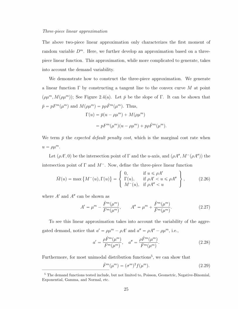
Three-piece linear approximation

The above two-piece linear approximation only characterizes the first moment of

random variable Dm. Here, we further develop an approximation based on a three-

piece linear function. This approximation, while more complicated to generate, takes

into account the demand variability.

We demonstrate how to construct the three-piece approximation. We generate

a linear function Γ by constructing a tangent line to the convex curve M at point

pρµm,Mpρµmqq; See Figure 2.4(a). Let p be the slope of Γ. It can be shown that

p “ pFmpµmq and Mpρµmq “ pρFmpµmq. Thus,

Γpuq “ ppu´ ρµmq `Mpρµmq

“ pFmpµmqpu´ ρµmq ` pρFm

pµmq.

We term p the expected default penalty cost, which is the marginal cost rate when

u “ ρµm.

Let pρA1, 0q be the intersection point of Γ and the u-axis, and pρA2,M´pρA2qq the

intersection point of Γ and M´. Now, define the three-piece linear function

Mpuq “ max

M´puq,Γpuq

(

“

$

&

%

0, if u ď ρA1

Γpuq, if ρA1 ă u ď ρA2

M´puq, if ρA2 ă u

,

.

-

, (2.26)

where A1 and A2 can be shown as

A1 “ µm ´Fmpµmq

Fmpµmq, A2 “ µm `

Fmpµmq

Fmpµmq. (2.27)

To see this linear approximation takes into account the variability of the aggre-

gated demand, notice that a1 “ ρµm ´ ρA1 and a2 “ ρA2 ´ ρµm, i.e.,

a1 “ρFmpµmq

Fmpµmq, a2 “

ρFmpµmq

Fmpµmq. (2.28)

Furthermore, for most unimodal distribution functions5, we can show that

Fmpµmq “ pσmq2fpµmq. (2.29)

5 The demand functions tested include, but not limited to, Poisson, Geometric, Negative-Binomial,Exponential, Gamma, and Normal, etc.

25

Thus, when the aggregated demand is more variable, a1 and a2 will be bigger (or

equivalently, A1 will be smaller and A2 will be bigger). Figure 2.4(a) depicts A1, A2,

a1, a2, two-piece linear function M´, and three-piece linear function M . The following

proposition formally establishes the lower bound systems.

Lemma 3. By replacing Mt with M´t (or Mt) in (2.23), the optimal cost of the

resulting model forms a lower bound to the optimal cost of the transformed m-model.

We refer to the resulting model with M´t (Mt) as the two-piece (three-piece)

lower bound. Clearly, the two-piece lower bound becomes the exact system if Dm is

deterministic. The following lemma shows the same result for the three-piece lower

bound if Dm follows a two-point distribution.

Lemma 4. If demand D follows a two-point distribution with probability mass PrtD “

ρA1u “ p{p and PrtD “ ρA2u “ 1´ p{p, then the three-piece linear function becomes

the exact cost function, i.e., Mpuq “ EDppu´ ρDq` “ Mpuq.

Figure 2.4: Linear approximations and optimal control policies

2.5.2 Lower Bound Solutions

To establish the lower bound solutions, it is opportune to define

w “ w ` ρEDmpRemq “ w ` ρµm.

26

We refer to w as the expected working capital level, which takes into account the

expected A/R during the m periods.

First, we derive the optimal solution to the two-piece lower bound. By replacing

Mt with M´t and substituting w , the default penalty becomes αmppy ´ wq`, which

shares the same structure as in (2.10). Therefore, under the same assumptions as

in Proposition 2, the pd, Sq policy is optimal for the two-piece lower bound. The

solid function in Figure 2.4(b) depicts the optimal base-stock level of this policy.

Equivalently,

y˚pwq “ pd_ wq ^ S. (2.30)

Next, we develop the optimal policy of the three-piece lower bound. By replacing

Mt with Mt and w with w, the transformed m-model in (2.23) and (2.24) becomes

Vtpx, wq “ minxďy

"

Htpyq ` αmMtpy ´ w ` ρµ

mt q ` α

mcpy ´ xq`αEVt`1py ´Dt, w ` θDt ` ρµt`m ´ ρµtq

*

, (2.31)

VT`1px, wq “ ´αmcx` αmEppw ` ρDm

T`1 ´ ρµmT`1q

´. (2.32)

We first state the myopic policy. Let d “ pd, dq and a “ pa1, a2q, then the optimal

policy consists of five control parameters pd, a, Sq. The firm implements a base-stock

policy with the optimal base-stock level dependent on the expected working capital

w (in inventory units). More specifically, let y˚pwq be the optimal base-stock, then,

y˚pwq “

$

’

’

’

’

&

’

’

’

’

%

d, if w ď d´ a2

w ` a2, if d´ a2 ă w ď d´ a2

d, if d´ a2 ă w ď d` a1

w ´ a1, if d` a1 ă w ď S ` a1

S, if S ` a1 ă w

,

/

/

/

/

.

/

/

/

/

-

. (2.33)

We next illustrate how these optimal control parameters are obtained. For fixed

w, the unconstrained myopic minimization problem at period t can be written as

vtpwq “ miny

gtpyq ` αmMtpy ´ w ` ρµ

mt q(

, (2.34)

where gtpyq “ Htpyq ` αmp1´ αqcy.

27

The optimal control parameters a1 and a2 are derived in (2.28); The default-

free base-stock St and default threshold dt can be derived from (2.14) and (2.15) by

replacing gtp¨q with gtp¨q and λ with m; We refer to dt as the expected default threshold,

which can be obtained from

dt “ sup

"

y :B

Bygtpyq ď ´α

mpt

*

. (2.35)

Let us define at “ a1t ` a2t . To solve the problem in (2.34), we consider five cases.

Case 1. When w ď dtá2t , the system’s expected working capital is lower than dtá

2t .

Now it is optimal to order up to threshold dt, and vtpwq “ Ltpwàtq`αmptat, where

Ltpwq “ ´αmppw ´ dt ´ a

1tq ` gtpdt ` a

1tq.

Case 2. When if dt ´ a2t ă w ď dt ´ a2t , the system’s expected working capital is

lower than dt ´ a2t . Now it is optimal to default by a2t in expectation, and vtpwq “

gtpw ` atq ` αmptat.

Case 3. When dt ´ a2t ă w ď dt ` a

1t, the system’s expected working capital is lower

than dt ` a1t. Now it is optimal to order up to threshold dt, and vtpwq “¯Ltpwq “

´αmptpw ´ dt ´ a1tq ` gtpdt ` a

1tq.

Case 4. When dtà1t ă w ď Stà

1t, the system is working capital constrained. Now

it is optimal to order up to w ´ a1t and leave no cash on hand in expectation. Thus,

vtpwq “ gtpw ´ a1tq.

Case 5. When St ` a1t ă w, the system has ample working capital and orders up to

the target base stock St. In this case, the expected cash balance will be nonnegative,

and vtpwq “ gtpStq.

We summarize the above five cases into the following proposition.

Proposition 3. The pd, a, Sq policy in (2.30) is optimal for the myopic problem in

(2.34).

28

As a result, equation (2.34) becomes

vtpwq “

$

’

’

’

’

&

’

’

’

’

%

Ltpw ` atq ` αmptat, if w ď dt ´ a

2t

gtpw ` atq ` αmptat, if dt ´ a

2t ă w ď dt ´ a

2t

¯Ltpwq, if dt ´ a2t ă w ď dt ` a

1t

gtpw ´ a1tq, if dt ` a

1t ă w ď St ` a

1t

gtpStq, if St ` a1t ă w

,

/

/

/

/

.

/

/

/

/

-

, (2.36)

and the critical ratio of the control parameter dt can be found in the following lemma.

Lemma 5. The expected default threshold dt satisfies

Ftpdtq “b´ αmpFm

t pµmt q ´ α

mp1´ αqc

h` b. (2.37)

Figure 2.5(a) depicts functions gp¨q, Lp¨q, ¯Lp¨q and vp¨q while solving the myopic

problem in (2.34). The slopes of the linear functions Lp¨q and ¯Lp¨q are ´αmp and

´αmp, respectively. Function vp¨q is shown as the bold convex curve connected by

five different functions (from the left to the right): the shifted linear function Lp¨q,

the shifted convex function gp¨q, linear function ¯Lp¨q, convex function gp¨q, and the

horizontal line.

Now, we show the optimality of the myopic policy. Similar to §2.4.2, we define

the “band” as

Bt “

pxt, wtq P <2| xt ď y˚t pwtq

(

.

Figure 2.5(b) depicts the optimal base-stock y˚ and band B, which is the area below

y˚.

We next explain how to derive the optimal policy. First, it is convenient to define

At “ Fmt pµ

mt q as a measure of asymmetry of demand Dm

t . In addition, recall the

definitions of A1 and A2 in (2.27). In analogy to §2.4.2, the following proposition

shows the optimality through decoupling.

Proposition 4. Assume that (1) Dt is stochastically increasing; (2) At is decreasing

in t; (3) both A1t and A2t are increasing in t. Then we have:

29

Figure 2.5: The optimal solution of the three-piece lower bound

(a) The control parameters dt, dt and St are non-decreasing in t and dt ď dt ď St

for all t;

(b) Vtpx, wq “ ´αmcx` Wtpwq for all t and px, wq P Bt, where

Wtpwq “ vtpwq ` αEWt`1pw ` θDt ` ρµt`m ´ ρµtq,

and WT`1pwq “ αmEppw ` ρDmT`1 ´ ρµ

mT`1q

´; Wtpwq is convex in w;

(c) The pd, a, Sq policy is optimal for the three-piece lower bound of the transformed

m-model.

Assumption (1) in Proposition 4 is similar to that in Proposition 2. Assumption

(2) requires, typically but not necessarily, that the aggregated demand Dmt is less

right-skewed when t gets larger. Note that most of the real life demand functions,

such as Poisson(λ) and Gamma(k, 1), are right-skewed and become more symmetric

under larger mean values (λ and k), hence satisfying Assumption (2). For zero-

skewed (or symmetric) distributions, such as Normal, the following lemma guarantees

Assumption (2) and (3). Moreover, most asymmetric demand distributions (Poisson,

Gamma, etc.) can be shown or tested to satisfy Assumption (3).

30

Lemma 6. If At is constant over t, then both A1t and A2t are increasing in t.

Proposition 4(c) shows the optimality of the (d, a, S) policy. As illustrated in Fig-

ure 2.5(b), the band is divided into two sub-regions by the expected default threshold

d: if the expected working capital level w ă d, the firm will order more than its

expected working capital (i.e., y˚pwq ě w). We call this over-order region. In the

over-order region, the firm takes advantage of the cash flow volatility and order more

aggressively. On the other hand, if w ą d, the firm will order less than its expected

working capital level and hold hold extra cash on expectation. We call this under-

order region. in the under-order region, the firm tries to avoid the cash flow risks

by ordering more conservatively. The over-order (under-order) deviation amount de-

pends on a2 (a1), which is proportional to the variance of the aggregated demand under

the same mean value. Notice that the binding region in the pd, Sq policy reduces to

a single point in the (d, a, S) policy where w “ d.

Similarly as in §2.4.2, we define the expected optimal default quantity as u˚pwq “

y˚pwq ´ w. The optimal pd, a, Sq remains the property that u˚pwq is increasing with

w, implying that lower (higher) working level leads to more aggressive (conservative)

inventory ordering decisions. This is consistent with the pd, Sq policy. However, the

optimal base-stock in the pd, a, Sq policy deviates from that of the pd, Sq policy in

different directions, due to the volatility of the stochastic cash inflow ρDm.

2.5.3 Heuristics

We develop two heuristic policies for the transformed m-model, basing on the two-

piece and three-piece lower bound systems. We refer to it as the pd, Sq and pd, a, Sq

heuristic, respectively. The control parameters can be obtained from (2.28), Lemma

1 and 5. There are three steps to implement the heuristic policy: first, observe w

and compute w; second, derive the optimal base-stock y˚ from (2.30) for the pd, Sq

policy, and y˚ from (2.33) for the pd, a, Sq policy; third, order inventory up to the

base-stock, or as close as possible.

31

To this end, we shall expect that the three-piece heuristic works better than the

two-piece heuristic, although the latter involves less control parameters, and thus is

easier to implement. The performance gap between these two heuristic policies gets

bigger when aggregated demand is more volatile. In practice, the two-piece heuristic

could serve as a simple substitute for the three-piece policy if the demand is less

variable.

2.6 Longer Collection Period (m ă n)

When the collection period is longer than the payment period, i.e., λ “ m ă n,

the firm has complete cash flow information up to λ periods plus known cash inflow

information from period t ` λ to t ` n. Unlike §2.4 and §2.5, here we define the

working capital level (excluding the extra receivables beyond t` λ) at the beginning

of period t as

w “ x` pw1 ´Peλ `Rλeλq{c,

where Rλt “ pRtń, ..., Rtń`λ´1q. Define the extra known accounts receivable as

R´λt “ pRtń`λ, ..., Rt´1q.

With these definitions and a similar analysis as in the previous sections, the in-

ventory decision for the base model in (2.6)-(2.7) can be determined by the following

dynamic program:

Vtpx,w,R´λt q “ min

xďy

Gtpx,w, yq ` αEVt`1py ´Dt, w `Rtń`λ{c´Dt,R´λt`1q

(

,

(2.38)

VT`1px,w,R´λT`1q “ ´α

λcx` αλpw´, (2.39)

where the single-period cost function Gtpx,w, yq is the same as in (2.10), and the

dynamic of R´λt is R´λ

t`1 “ pRtń`1, ..., Rtń`λ´1, rDtq.

We refer to (2.38) and (2.39) as the transformed n-model. Denoting band Bt the

same as in (2.18), we show the optimal policy in the following proposition.

Proposition 5. If Dt is stochastically increasing, then we have:

32

(a) The control parameters dt and St are non-decreasing in t and dt ď St for all t;

(b) Vtpx,w,R´λt qq “ ´α

λcx `Wtpw,R´λt qq for all t and px,wq P Bt, where Wt is

joint convex;

(c) The pd, Sq policy is optimal for the transformed n-model.

Proposition 5 suggests that the extra cash flow information R´λt does not affect

the inventory decisions. Therefore, the optimal policy is the same as that for the

transformed λ-model.

2.7 Numerical Study

§2.7.1 examines the effectiveness of the heuristics. §2.7.2 discusses the impact of

payment periods on the system’s total cost. §2.7.3 measures the bullwhip effect

driven by the customer payment default.

2.7.1 Effectiveness of the Heuristics

The Heuristics for the Model with a Longer Payment Period

Here we test the performance of the pd, Sq and pd, a, Sq heuristics in §2.5.3. Both

heuristics are compared to the three-piece lower bound of the transformed m-model

developed in §2.5.1. We conduct an individual test for m “ 1, 2, 3, and summarize

the overall performances. In each test, let C2 be the cost of the pd, Sq heuristic based

on the two-piece linear approximation, and C3 be the cost of the pd, a, Sq heuristic

based on the three-piece linear approximation. Furthermore, let C3 be the cost of the

three-piece lower bound, then the percentage errors are defined as

% error-2 “C2 ´ C3

C3

ˆ 100%, % error-3 “C3 ´ C3

C3

ˆ 100%.

We consider two demand forms. For the i.i.d. demand case, Dt is Normal dis-

tributed with mean µt “ 10 for all t; for the increasing demand case, Dt is Normal

33

distributed with the first period mean µ1 “ 10 and µt increasing at a rate of 10%

per period. We fix the working capital requirement policy with r taking two values:

r “ p1, 1.1q. Moreover, the initial working capital level can also vary between two val-

ues: w1 “ p20´ 10m, 10´ 10mq, i.e., the leftover A/P from the last planning horizon

is considered at period 1. In addition, we fix parameters c “ 1, α “ 1, and vary the

other parameters with each taking two values: h “ p0.05, 0.2q, b “ p1, 4q, p “ p0.5, 2q

. The total number of instances generated for each heuristic is 384. The average

(maximum, minimum) performance error for the pd, Sq heuristic is 2.12% (21.23%,

0.00%), and that for the pd, a, Sq is 1.46% (13.21%, 0.00%). As expected, the pd, a, Sq

heuristic performs well in general, and the performance difference between these two

heuristic policies is higher when demand becomes more variable.

Negative Demand Shocks

Recall from §2.4.2 and §2.6 that the pd, Sq policy is shown to be optimal for the trans-

formed λ-model and the transformed n-model, respectively. In addition, §2.5.2 shows

that the pd, a, Sq policy is optimal for the three-piece lower bound of the transformed

m-model. All these results were proved under the assumption of stochastically in-

creasing demand. With the existence of negative demand shocks, the above optimal

policies become heuristics. In what follows we test the effectiveness of these heuristics

under different non-stationary demand forms with negative shocks.

We conduct an individual test for each of the three models mentioned above and

summarize the overall heuristic performance. In each test, let CU be the cost of the

heuristic which serves as an upper bound cost for the underlined model. We compare

CU with a lower bound cost CL obtained by relaxing the constraint x ď y in each

period, i.e., the feasibility of the optimal base-stock level is guaranteed by allowing

inventory return at the purchasing cost. To evaluate the heuristic, we define the

percentage error as

% error “CU ´ CLCL

ˆ 100%.

34

Our numerical study starts with a test bed which has the time horizon of 12

periods. We fix parameters λ “ 0, m “ 1, n “ 1. In addition, we consider two

demand forms with negative shocks: seasonal demand and product life cycle demand.

In each demand form, Dt is normally distributed with mean µt shown in Table 2.2.

In our text bed, the demand coefficient of variation (c.v.) can vary by taking two

values: c.v.“ p0.15, 0.3q. We also consider two working capital requirement policies.

For the fixed policy, we set rt “ 1 for all t; for the responsive policy, rt is non-

stationary with values set according to Table 2.2. Finally, we assume the initial

on-hand inventory x1 “ 10 and vary the initial working capital level between two

values: w1 “ p10, 40q. The values of other parameters remain the same as in the

test bed of “the heuristics for the model with a longer payment period”. In total, we

generate 384 instances. The combination of these parameters covers a wide range of

different system characteristics.

Table 2.2: Demand mean and responsive working capital requirement

Period ptq 1 2 3 4 5 6 7 8 9 10 11 12µt - seasonal demand 10 12 20 60 20 12 10 12 20 60 20 12rt - seasonal demand 1.2 1.2 1.5 0.8 0.8 1.0 1.2 1.2 1.5 0.8 0.8 1.0µt - life cycle demand 10 12 14 18 22 38 50 56 60 52 36 8rt - life cycle demand 1.2 1.2 1.2 1.2 1.2 1.2 1.2 1.2 0.8 0.8 0.8 0.8

The average (maximum, minimum) performance error for the test bed instances

is 0.36% (4.63%, 0.00%). When negative shocks exist in the demand sequence, the

underlined heuristics perform well in general. Nevertheless, the heuristics perform

less effectively when both the c.v. and the backorder cost are large. To see this, recall

from Proposition 2 that the myopic policy is optimal under the condition that the

states will stay within the band if they are already in the band. When demand is

expected to drop, the optimal base-stock level will decrease accordingly. Therefore, it

is probable that a small demand realization will cause the states traverse outside the

35

band, making the heuristic less effective. This is more likely when demand is more

variable and there is a bigger decrease in base-stock levels. The latter is mainly due

to a higher backorder cost.

2.7.2 Impact of Payment Periods

Although the firm may benefit from a longer purchases payment period, the supplier

will usually quote a higher unit wholesale price to compensate for the postponed cash

inflow. This price increase can be regarded as the implicit cost of trade credit for

the firm. To fully understand this tradeoff, the firm needs to analyze the cost saving

from extending the payment period. In this subsection we conduct a numerical study

to illustrate the impact of payment periods on the firm’s total cost, thus providing a

decision support tool in the trade credit contract negotiation.

In our numerical study, we compute the percentage cost reduction achieved by

the model with m “ 1 over that with m “ 0. To obtain the true value of this cost

reduction, we keep the unit purchasing cost c unchanged. The underlined model and

policy differ with respect to the length of the collection period. When n “ 0, we use

the pd, a, Sq heuristic of the transformed m-model to compute the cost with m “ 1,

and the pd, Sq policy of the transformed λ-model (λ “ 0) for the cost with m “ 0;

when n “ 1, we use the pd, Sq policy of the transformed n-model for the cost with

m “ 0, and the same policy of the transformed λ-model (λ “ 1) for the cost with

m “ 1.

We consider a planning horizon of 12 periods with the initial states x1 “ 10 and

w1 “ 20.6 Demand is Normal distributed with mean in the first period µ1 “ 10 and

µt is increasing at a constant rate. In addition, we set r “ 1, α “ 1, and h “ 0.05.

We study the impact of payment delays on cost reduction under different system

parameters and summarize the results in Figure 2.6. In particular, Figure 2.6(a)

plots the percentage cost reduction curve with respect to the c.v. of the demand, and

6 Similar to the last section, in the case of m “ 1, w1 needs to be adjusted to consider the leftoverA/P from the last planning horizon.

36

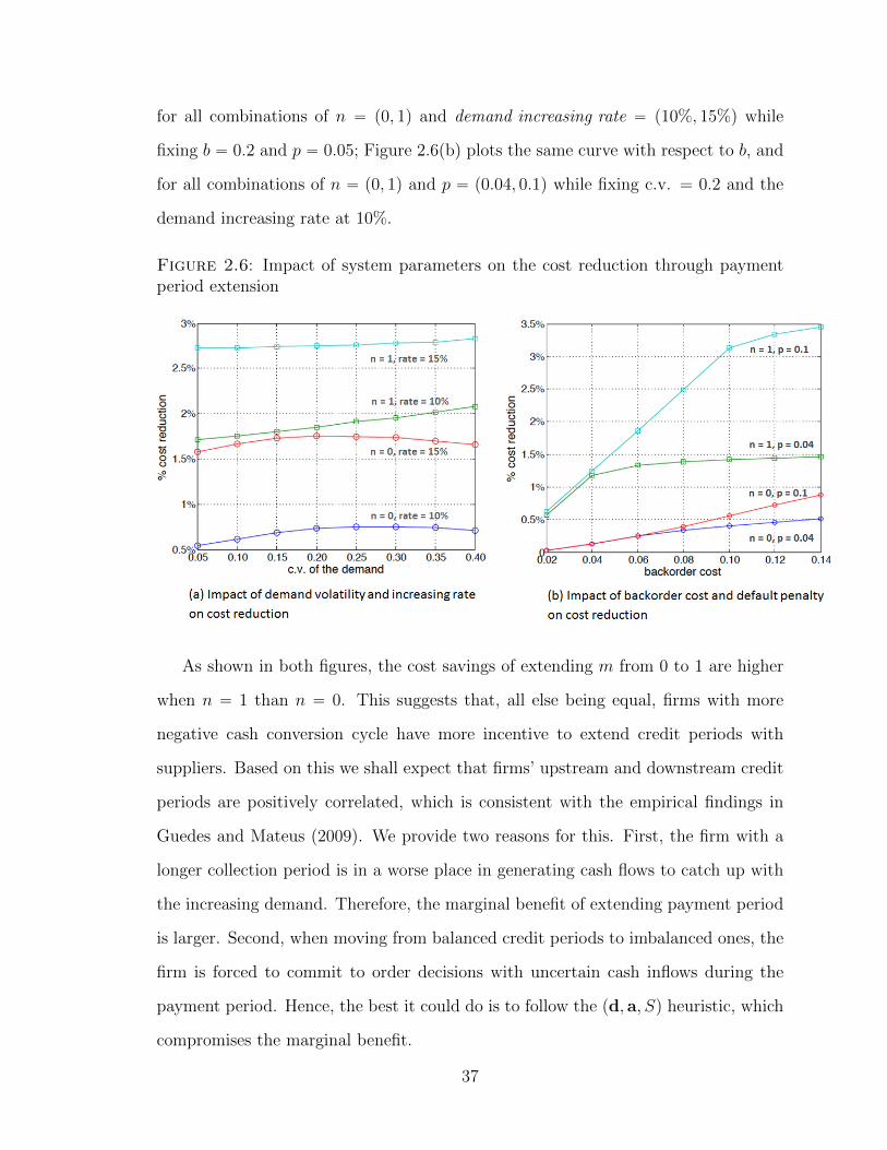
for all combinations of n “ p0, 1q and demand increasing rate “ p10%, 15%q while

fixing b “ 0.2 and p “ 0.05; Figure 2.6(b) plots the same curve with respect to b, and

for all combinations of n “ p0, 1q and p “ p0.04, 0.1q while fixing c.v. = 0.2 and the

demand increasing rate at 10%.

Figure 2.6: Impact of system parameters on the cost reduction through paymentperiod extension

As shown in both figures, the cost savings of extending m from 0 to 1 are higher

when n “ 1 than n “ 0. This suggests that, all else being equal, firms with more

negative cash conversion cycle have more incentive to extend credit periods with

suppliers. Based on this we shall expect that firms’ upstream and downstream credit

periods are positively correlated, which is consistent with the empirical findings in

Guedes and Mateus (2009). We provide two reasons for this. First, the firm with a

longer collection period is in a worse place in generating cash flows to catch up with

the increasing demand. Therefore, the marginal benefit of extending payment period

is larger. Second, when moving from balanced credit periods to imbalanced ones, the

firm is forced to commit to order decisions with uncertain cash inflows during the

payment period. Hence, the best it could do is to follow the pd, a, Sq heuristic, which

compromises the marginal benefit.

37

Figure 2.6 also shows that the cost reduction increases with the backorder cost,

the default penalty, and the demand increasing rate. This is because the higher these

parameters are, the more cost firms will incur by not being able to catch up with the

increasing demand due to negative cash conversion cycles. Therefore, there is more

incentive to enhance the cash flow by extending the payment period. Interestingly, the

cost reduction is not monotone in demand volatility when n “ 0, as shown in Figure

2.6(a). To see this, note that a higher c.v. will lead to higher control thresholds, and

possibly to a higher base-stock level, which will increase the potential benefit of a

longer payment period. However, the demand volatility also makes it harder to make

inventory order decision when m ą n due to the uncertainty of future cash inflows.

When c.v. is large enough, the latter effect will dominate the former one, making it

less attractive to extend the payment period.

2.7.3 Bullwhip Effect

Bullwhip effect is a phenomenon that the order variability amplifies when moving

along the supply chain from downstream to upstream (Lee et al., 1997). In this stream

of literature it has been shown that imposing finite capacity to the system does not

cause bullwhip effect. Two different types of capacities are considered: for the shelf

capacity, order variability equals to the demand variability7; for the production/order

capacity, order variability is less than the demand variability, i.e., the smoothing effect

(Chen and Lee, 2012). In our original model, the on-hand cash can be regarded as

a random and endogenous capacity. After the transformation, the working capital

level becomes an exogenous shelf capacity. When customers do not default on trade

credit, we should not be able to observe bullwhip effect under stationary demand and

fixed working capital requirement r “ 1. However, when there is a customer payment

default, the working capital level becomes more variable, which may amplify the order

variability and cause the bullwhip effect.

7 In this case, the order sequence will replicate the demand sequence.

38

To further understand this driver of bullwhip effect, we extend our model to

incorporate customer payment defaults. More specifically, we model the doubtful

receivable of age t´ n as follows

Rtń “ pδtRtń ` εtq`, (2.40)

where Rtń is the expected full payment according to (2.4), δt P r0, 1s is the estimated

proportion of collectible amount, and εt is a random variable representing the payment

default uncertainty. We assume εt is independent from period to period with mean

µt and variance σ2t . To measure the bullwhip effect, we conduct a simulation study

with m “ n “ 0 over 36 periods. The demand is Normal distributed with stationary

mean µ “ 10 and standard deviation σ “ 2. In addition, we assume that the default

noise εt also follows an i.i.d Normal distribution with µ “ 0 and σ varying from 0 to

4. Finally, we set δ “ 1, r “ 1, α “ 1, x1 “ w1 “ 10, b “ 0.4 and vary p to take

values at 0, 0.2, and 0.4. This set of system parameters allow us to study the impact

of customer default volatility and default penalty cost on the bullwhip ratio, which

is defined as the ratio between order variance and demand variance.

Figure 2.7: Customer payment default and bullwhip effect

39

Figure 2.7(a) and (b) plot the sample path of working capital level under the

parameter combination pp, σq “ p0.2, 1q and p0.4, 2q, respectively. Following the pd, Sq

policy, the optimal base-stock level in period t equals to wt if d ă wt ď S. As wt

varies due to customer payment defaults, the order sequence will no longer replicate

the demand sequence. Rather, the order quantity will become more variable, making

the bullwhip ratio larger than 1. When wt travels below d (above S), the optimal

base-stock is fixed at d (S). And consequently, the order variance will reduce to

the demand variance. Therefore, the area between d and S is where the customer

payment defaults can effectively drive the bullwhip effect. As shown in 2.7(c), the

bullwhip ratio increases in both the customer default volatility σ and the default

penalty cost p. As p approaches to b, d approaches to negative infinity, in which case

the bullwhip effect is the most significant.

As illustrated in Figure 2.7(c), a smaller default penalty cost p leads to a lower

bullwhip ratio. When p decreases, the firm will default more, which implies that the

supplier could effectively mitigate the bullwhip effect through liquidity provision. In

this sense, we suggest another rationale for suppliers to provide trade credit when

banks do not.

2.8 Conclusion

This chapter studies the impact of trade credit on a firm’s inventory decision. The

firm provides and receives one-part trade credit contracts. We introduce a notion of

working capital that simplifies the computation and characterizes the optimal and

near-optimal policies. This result naturally connects operations and accounting. Our

analysis reveals insights on the relationship between the payment period and the

resulting procurement cost and on how supplier’s liquidity provision can mitigate the

bullwhip effect.

40

3

Joint Inventory and Cash Management

This chapter develops a centralized supply chain model that aims to assess the value

of cash pooling. The supply chain is owned by a single corporation with two divisions,

where the downstream division (headquarter), facing random customer demand, re-

plenishes materials from the upstream one. The downstream division receives cash

payments from customers and determines a system-wide inventory replenishment and

cash retention policy. We consider two cash management systems that represent dif-

ferent levels of cash concentration. For cash pooling, the supply chain adopts a

financial services platform which allows the headquarter to create a corporate master

account that aggregates the divisions’ cash. For transfer pricing, on the other hand,

each division owns its cash and pays for the ordered material according to a fixed

price. Comparing both systems yields the value of adopting such financial services.

We prove that the optimal policy for the cash pooling model has a surprisingly sim-

ple structure – both divisions implement a base-stock policy for material control; the

headquarter monitors the corporate working capital and implements a two-threshold

policy for cash retention. Solving the transfer pricing model is more involved. We

derive a lower bound on the optimal cost by connecting the model to an assembly

system. Our results show that the value of cash pooling can be very significant when

41

demand is increasing (stationary) and the markup for the upstream division is small

(high). Nevertheless, a big portion of the pooling benefit may be recovered if the

headquarter can decide the optimal transfer price and the lead time is short.

3.1 Introduction

The fundamental objective of supply chain management is to efficiently coordinate

material, information, and financial flows so as to reduce mismatches between demand

and supply. When financial markets are efficient, i.e., external funding is plentiful and

relatively inexpensive, the financial decisions may be decoupled from the logistics deci-

sions (Modigliani and Miller, 1958). In such case, a downstream party pays material it

orders from an upstream one so financial flow becomes an output of logistics decisions.

This perspective may explain why the supply chain literature has largely focused on

the integration of material and information flows. Nonetheless, with the recent global

financial crisis limiting the availability of external funding, many multinational, multi-

divisional corporations in their “hunt for cash” have witnessed a significant increase

on their intragroup financial transactions (Rogers et al., 2009). The reason is sim-

ple: these multinationals realize that they can concentrate the intragroup liquidity

for centralized planning to receive most benefit. For example, Hewlett-Packard and

General Electric transfer funds from their overseas divisions to their domestic ones

by considering the benefit of the entire company group. (Linebaugh, 2013). One

of the common practices of cash concentration is cash pooling (Polak and Klusacek,

2010). Under cash pooling, the headquarter creates a corporate master account that

aggregates division’s cash on a daily basis (Jansen, 2011). While the value of cash

pooling has been studied in the finance literature, there is little study that assesses

the value from a supply chain perspective. Indeed, the discussion of integrating finan-

cial flows into supply chain models is relatively sparse in the supply chain literature.

The objective of this paper is to fill this gap.

We consider a corporation that owns a supply chain consisting of two divisions

42

(can be generalized to N divisions). The downstream division, division 1, replenishes

inventory from an upstream division, division 2, which further replenishes from an

outside ample vendor. There are positive delivery lead times for both divisions.

Division 1 is the headquarter that faces stochastic customer demand. The demands

are independent between periods but not necessarily identical. Division 1 receives cash

payment from customers who order the material. Similarly, division 2 pays to the

outside vendor for the material shipped to the division. To make the consideration of

financial flow relevant, we assume that there is no external borrowing. The decision is

centralized and the headquarter has to decide a system-wide inventory replenishment

and cash retention policy. The cash retention policy refers to how much cash the

supply chain should hold for operations, i.e., inventory payments in our context.

Typically, firms do not wish to hold excess cash as it loses the potential benefit from

external investments; on the other hand, liquidating invested assets into cash for

operations incurs transaction costs or may not be feasible (Baumol, 1952; Miller and

Orr, 1966). Thus, the headquarter has to find a balance of amount of cash between

retained for internal operations and invested for external assets.

We consider two cash management systems that represent different levels of cash

concentration. For the cash pooling system, the supply chain adopts a financial ser-

vices platform, so the entire supply chain is operated under a single account for

conducting financial transactions with customers and the outside vendor. For the

transfer pricing system, no such platform is installed so each division maintains its

own cash and division 1 pays exactly what it orders to division 2 according to a fixed

internal transfer price, i.e., the price that a selling division charges for a product or

service supplied to a buying division of the same corporation (Abdallah, 1989). We

assume that the transfer price is pre-determined according to a market price (Mar-

tini, 2011). There are linear holding and backorder costs related to the inventory. In

addition, there is an opportunity cost for holding cash, which represents the oppor-

tunity cost of holding cash for internal operations. The objective is to find a joint

43

inventory replenishment and cash retention policy such that the total supply chain

cost is minimized within a finite horizon under each of the cash management systems.

The logistics system of the considered supply chain is a seminal model proposed

by Clark and Scarf (1960). We incorporate cash flows into this classical model.

The transfer pricing model represents a traditional supply chain in the sense that

cash payment is driven by the inventory decision (constrained by the available cash).

Thus, cash may not be efficiently distributed, leading to a less effective inventory and

cash retention policy. For example, cash shortage of the upstream division will affect

its normal operations, which, in turn, affects the material supply to the downstream

one. This inefficiency can be mitigated under cash pooling because the headquarter

can consolidate the cash within the supply chain for a better usage. In practice,

there are physical pooling and notional (virtual) pooling (i.e., funds are not physically

transferred but managed as if they were in a single account). In any case, cash pooling

usually involves financial and legal services provided by a third party and requires

installing a costly system-wide technology platform, such as treasury management

system, for transferring funds from divisions to the headquarter (Camerinelli, 2010).

Thus, our study of comparing these two systems can be used to justify the value of

adopting such financial services.

We first formulate a dynamic program for the cash pooling model which includes

two inventory states and one cash state that represents the corporate master ac-

count. To be consistent with the inventory literature, we name division and stage

interchangeably. The problem is difficult to solve as one cannot directly prove a

structured joint optimal policy. Nevertheless, by redefining the state variables into

echelon terms, we can transform the original two-stage system into a three-echelon

system, under which the optimal joint policy can be characterized. The optimal pol-

icy is surprisingly simple. The inventory policy has the same structure as that for

the traditional multi-echelon system (cf. Clark and Scarf, 1960): each stage reviews

the echelon inventory position at the beginning of a period and orders up to a target

44

echelon base-stock level. For the cash retention policy, stage 1 (or the headquarter)

reviews the entire system working capital (= inventory on hand at both stages +

inventory in transit - backorders at stage 1 + inventory-equivalent total system cash)

at the beginning of each period and retain the cash holding within an interval. A

technical contribution for this model is that we simplify the computation by decou-

pling the original dynamic program with three states into three separate dynamic

programs, each with one state variable. Thus, the optimal policy parameters can be

easily found. The decoupling result is based on a set of penalty cost functions, some

appearing to be new in the literature. We also provide economic meanings for these

penalty functions.

Solving the transfer pricing model is more involved. Simply speaking, the problem

is similar to a serial capacitated system (cf. Parker and Kapuscinski, 2004) in the sense

that the on-hand cash level at each stage can be viewed as a budgetary constraint that

restricts the amount of inventory ordering. However, the major difference between the

traditional capacitated system and ours is that the cash constraint is endogenously

determined by the inventory and cash retention decisions. Although we are not able

to characterize the optimal policy, we provide a lower bound to the optimal cost by

connecting the transfer pricing model to an assembly system (cf. Rosling, 1989) with

two component flows – one is stage 1’s cash flow and the other is the system’s material

flow.

We obtain several insights from the above analysis. First, the optimal policy of the

cash pooling model suggests that the inventory decision can be made separately from

the cash retention decision; however, making the cash retention decision has to take

into account the entire supply chain inventory. That is, monitoring system working

capital level is key to ensuring the system efficiency. In most firms, cash payment is

managed by a treasurer in the accounting department, and replenishment decision is

made by an inventory manager in the operations department. A implication of our

finding is that a close inter-departmental collaboration is crucial. Second, comparing

45

the optimal cost of the cash pooling model and the lower bound cost of the transfer

pricing model renders the (conservative) value of cash pooling, or equivalently, in-

stalling the financial services platform. Our numerical result suggests that the value

of cash pooling can be very significant when the profit margin of the upstream stage

is low and the demand is increasing or when the profit margin is high and the demand

tends to be stationary. For the former case, the upstream division tends to have cash

shortage in the transfer pricing model. Lacking cash at the upstream stage restricts

the order quantity, which affects the material supply for the downstream stage. On

the other hand, for the latter case, there is excess cash accumulated in the upstream

division. Pooling cash together will facilitate the headquarter to invest the excess

cash to external opportunities. Third, we compare the optimal cost of the cash pool-

ing model to that obtained from the Clark-Scarf algorithm. We find that ignoring

the impact of financial flow can be significantly suboptimal.

The above comparison leads to an interesting question: If the headquarter can

determine the internal transfer price for the divisions, how much benefit can be re-

covered by employing the optimal transfer price? Determining transfer prices is one

of the most controversial topics for multi-divisional firms in the finance literature.

When an inventory manager attempts to determine the optimal flows of products

among divisions, the price of a product is almost always considered a given param-

eter, as the setting in the transfer pricing model. However, this is not the case in

real multi-divisional firms since the transfer price is inherently subjective and the

headquarter can determine it with some degree of flexibility through advance pricing

agreements (Vidal and Goetschalckx, 2001; Lakhal, 2006; Perron et al., 2010; Martini,

2011)1. Thus, one can treat transfer pricing as a tool of re-distributing cash between

1 Our focus is to determine the system-wide optimal transfer price. Certainly, an optimal transferprice may not be aligned with each division’s best interest, so there is a separate issue regarding howto implement the optimal transfer prices for the divisions. However, if implementing the optimaltransfer price decreases the supply chain’s cost, the headquarter can capture this benefit and designa incentive compatible compensation, such as side payment, that induces the division to accept theprice.

46

divisions (Stewart, 1977). We call the system with optimized internal transfer price

as the optimal pricing system. The optimal transfer price can be determined if we

obtain the optimal order quantity and the optimal cash payment between these two

divisions in each period (i.e., transfer price is equal to cash payment divided by order

quantity)2. In other words, we need to obtain an optimal joint inventory replenish-

ment, cash payment, and cash retention policy for the supply chain. Interestingly, we

find that this joint optimal policy can be obtained by extending the solution approach

for the cash pooling model. More specifically, the inventory replenishment and cash

retention policy structure remains the same as those in the cash pooling system; for

the payment policy between divisions, division 2 monitors its echelon working capital

level and receives the cash payment up to a target level.

The optimal pricing model allows us to gain additional insights. While the cash

pooling system certainly dominates the optimal pricing one, we find that the supply

chain can recover a big portion of the cash pooling benefit by optimizing the transfer

price. The benefit of re-distributing liquidity through the optimal transfer price can be

clearly demonstrated in a product life cycle example in §3.5: during the introduction

and growth stages, the upstream division is normally short of cash so cash subsidy

from the downstream stage is valuable. On the other hand, during the mature and

decline stage, division 2 has accumulated sufficient fund for the decreased demand,

so a reduction of cash payment from division 1 is beneficial. Finally, we investigate

material and cash bullwhip effects (i.e., shipment and payment variability) under

the optimal pricing and transfer pricing systems. We find that the variability of

cash payment from division 1 to the division 2 is larger (smaller) than that from

the division 2 to the outside vendor under the optimal pricing (transfer pricing)

system. On the other hand, the variability of inventory shipment grows when moving

upstream under both schemes. Thus, the material and financial bullwhip effects may

2 In our context, the optimal cash payment between two divisions can broadly include intragrouploans or financial subsidies.

47

not amplify in the same direction in a fully integrated supply chain. Comparing the

material bullwhip between these systems, we find that the material bullwhip effect

is less significant under the optimal pricing system. This implies that an effective

transfer price policy can be a useful tool to mitigate the material bullwhip effect.

3.2 Literature Review

Our work is related to four streams of research in the literature: cash management,

multi-echelon inventory models, capacitated inventory models, and inventory model

with financial issues.

For cash management in single firms, most papers treat cash as inventory and use

inventory control tools to find the optimal cash balance for firms. Baumol (1952)

studied the optimal cash level for a firm that uses cash either for paying transactions

or for investment. We have a similar setup for the headquarter in our model. This

line of research was further extended by Tobin (1956) and Miller and Orr (1966). For

dynamic, periodic-review cash balance problems, Girgis (1968) modeled the selection

of a cash level in anticipation of future net expenses as a single-product, multi-period

inventory system. Heyman (1973) presented a model to minimize the average cash

balance subject to a constraint on the probability of stock-out. The difference between

these studies and ours is that we specifically model the cash and inventory dynamics

as two inter-related flows.

For cash management in multi-divisional corporations, our model is related to

resource allocation from a centralized planning perspective. This literature can be

categorized into two groups. The first group is related to cash pooling. Eijie and

Westerman (2002) suggested that the reduction of financial imperfections in trans-

ferring cash in the euro zone diminishes the need for separate local cash holdings

and facilitates the cash concentration and headquarter’s financial control. We refer

the reader to Jansen (2011) for a detailed discussion on cash pooling concepts and

practices surveyed in fifteen countries. The second group concerns obtaining transfer

48

prices to maximize the profit for a multi-divisional corporation, e.g., Merville and

Petty (1978), Vidal and Goetschalckx (2001), Gjerdrum et al. (2002), Lakhal (2006),

Villegas and Ouenniche (2008), and Perron et al. (2010). Our model is different from

these papers in that we consider a supply chain setting in a finite horizon and charac-

terize the optimal control policy. There is another stream of research regarding how

to design transfer prices to coordinate decentralized divisions (i.e., each division has

high autonomy and is treated as a profit center). Since the focus is different from our

paper, we refer the interested reader to Ronen and McKinney (1970) and Yeom et al.

(2000).

Our research is also related to the multi-echelon literature. In particular, our

model incorporates cash flows into the seminal supply chain model developed by Clark

and Scarf (1960), who proved that an echelon base-stock policy is optimal. Further-

more, they showed that the problem can be decoupled into a series of one-dimensional

dynamic programs by introducing the notion of echelon inventories. Federgruen and

Zipkin (1984) and Chen and Zheng (1994) streamlined the analysis by considering an

infinite horizon model. Recently, Angelus (2011) considered a multi-echelon model

which allows each stage to dispose excess inventory to a secondary market. He intro-

duced a class of heuristic policies, called disposal saturation policies, which can be

obtained by using the Clark-Scarf decomposition.

The capacitated inventory problem is related to our model since the cash con-

straint on inventory replenishment can be viewed as the supply capacity. For single-

stage systems, Federgruen and Zipkin (1986) showed that the modified base-stock

policy is optimal. Angelus and Porteus (2002) derived the optimal joint capacity ad-

justment and production plan with and without carryover of unsold inventory units.

Their capacity adjustment decision is similar to our cash investment decision, but

our cash capacity is also affected by payment decisions and random sales. For serial

systems, Parker and Kapuscinski (2004) demonstrated that a modified echelon base-

stock policy is optimal in a two-stage system where there is a smaller capacity at the

49

downstream facility. Glasserman and Tayur (1995) and Huh et al. (2010) studied the

stability issue of the system. The main difference between the serial capacitated mod-

els and ours is that the cash constraint is endogenously determined by the inventory

and cash decisions.

Finally, there have been several recent studies to incorporate financial decisions

or budget constraints into inventory models. Most of these papers are based on

single-stage systems. Buzacott and Zhang (2004) incorporated asset-based financing

into production decisions. They demonstrated the importance of joint consideration

of production and financing decisions to capital constrained firms. Li et al. (2013)

studied a dynamic model in which inventory and financial decisions are made simul-

taneously in the presence of uncertain demand. The objective is to maximize the

expected present value of dividends. The authors proved that a myopic policy is

optimal. Ding et al. (2007) studied an integrated operational and financial hedging

decision faced by a global firm which sells to both home and foreign markets. Chao

et al. (2008) considered a self-financing retailer who replenishes inventory under a

cash budget constraint. They characterized the optimal inventory control policy.

Gupta and Wang (2009) presented a discrete-time inventory model with trade credit

and showed that the problem can be converted into a single-stage system model

with refined holding cost rates. Babich (2010) studied a manufacturer’s joint inven-

tory and financial subsidy decisions when facing a supplier whose financial state is

governed by a firm-value model. He showed that an order-up-to policy and subsidize-

up-to policy are optimal for the manufacturer. Yang and Birge (2011) modeled a

Stackelberg game between a retailer and a supplier with the use of a trade credit

contract. They demonstrated that an effective trade credit contract can enhance

supply chain efficiency. Bendavid et al. (2012) analyzed the material management

practices of a self-financing firm under working capital requirement. Tanrisever et al.

(2012) built a two-period model to study a start-up firm’s trade-off between process

investment and survival. For multi-echelon models, Hu and Sobel (2007) studied a

50

serial inventory model with the objective of optimizing the expected present value of

dividends. They showed that there is no optimal echelon base-stock policy if there

are financial constraints. Protopappa-Sieke and Seifert (2010) conducted a simula-

tion study on a two-stage supply chain to reveal qualitative insights on the allocation

of working capital between the supply chain partners. Chou et al. (2013) studied a

one-warehouse-multi-retailer system with trade credits.

The rest of this paper is organized as follows. §3.3 studies the cash pooling model

and formulates the corresponding dynamic program. §3.4 focuses on the transfer

pricing model. We provide lower bounds to the optimal cost. §3.5 discusses the

qualitative insights through a numerical study. §3.6 concludes. Appendix provides

proofs. Throughout this paper, we define x` “ maxpx, 0q, x´ “ ´minpx, 0q, a_ b “

maxpa, bq, and a^ b “ minpa, bq.

3.3 Cash Pooling System

We consider a periodic-review, two-stage serial supply chain where stage 1 orders

from stage 2, which orders from an outside ample vendor. The supply chain is owned

by a single corporation, with stage 1 being the headquarter and stage 2 the sub-

sidiary. Stage 1 faces a stochastic customer demand Dt in period t. The demands are

independent between periods, but the demand distributions may differ from period

to period. We assume that unsatisfied demand is fully backlogged, and the material

lead time is one period for both stages (without loss of generality).

This section focuses on the cash pooling (CP) system, in which the headquarter

(stage 1) creates a corporate master account that aggregates the divisions’ cash and

pays for the outside vendor. Here and in the sequel, we use prime to indicate local

(stage specific) variables and parameters. To model the opportunity cost of holding

cash, let rf be the risk-free rate of investment, and R the overall return rate for the

headquarter’s investment activities, where R ě rf . Assuming risk neutrality, the

opportunity cost of holding cash can be expressed as η1 “ R ´ rf . We refer to η1

51

as cash holding cost rate. Moreover, we assume the headquarter can liquidate its

assets to assist inventory payment, if necessary. Nevertheless, how much cash can

flow into the pooled account depends on an exogenous market condition described

by a limit K1

pě 0q in each period3. Let β1

i and β1

o denote the unit transaction cost

charged on the cash transferred to and from the pooled cash account, respectively. In

practice, these transaction costs can be regarded as brokerage fees. Here, β1

i, β1

o and

K1

represent the market friction in this model. Figure 3.1 shows the material and

cash flows in solid and dashed arrows, respectively. The circle in Figure 3.1 represents

the investment portfolio; the top white rectangle represents the pooled cash balance,

or the operating account.

Figure 3.1: The two-stage cash pooling model with material and cash flows

We now introduce the other cost parameters. Following the inventory literature,

we charge a linear local holding cost h1

i for each unit of inventory held at stage i in

each period, and a backorder cost b for each unit of backorder incurred at stage 1 in

each period. Here, we assume that h1

1 ą h1

2 ą η1

c, i.e., holding a unit of inventory at

downstream is more costly than that at upstream, and holding an unit of inventory

is more costly than holding the same value amount of cash. The later is generally

true since inventory holding cost consists of both the financial opportunity cost and

the physical shelf cost.

The inventory replenishment and cash retention decision is made centrally by the

headquarter. The sequence of events in a period as follows: At the beginning of

3 The sequence of K1

t can be generalized to a Markov chain that captures the stochastic liquiditylevel according to the market condition.

52

the period, (1) shipments are received at both stages; (2) payment is made to the

outside vendor; (3) cash retention decision is made; (4) orders are placed at both

stages. During the period, demand is realized and sales revenue is collected. At the

end of the period, all inventory and cash related costs are calculated. The planning

horizon is T periods, and the objective is to minimize the supply chain’s total expected

discounted cost within the entire horizon.

We now define state and decision variables. For stage i “ 1, 2 and period t, let

x1

1,t “ net inventory level at stage 1 after Event (1);

x1

2,t “ on-hand inventory level at stage 2 after Event (1);

w1

t “ cash balance in the pooled account after Event (2);

vt “ amount of cash transferred into the pooled account in Event (3);

zi,t “ order quantity for stage i made in Event (4);

Note that v`t is the cash amount that flows into the pooled account and v´t is the

cash amount that flows out for investment. Clearly, vt cannot exceed K1

. Let p1 be

the unit selling price to the end customer and c be the unit procurement cost from

the outside vendor. We assume c ă p1 to ensure profitability. The system dynamics

are shown below:

x1

1,t`1 “ x1

1,t ` z1,t ´Dt, (3.1)

x1

2,t`1 “ x1

2,t ` z2,t ´ z1,t, (3.2)

w1

t`1 “ w1

t ` vt ´ cz2,t ` p1Dt. (3.3)

We assume that the actual payment transaction occurs upon the receipt of ship-

ments. That is, the outside vendor will not receive the payment determined in period

t until period t ` 1, when stage 2 receives the shipment (placed in period t). This

payment practice is similar to a Letter of Credit (LC). In other words, we can view

that there is a one-period lead time for the cash payment.

For the cash dynamic in (3.3), we assume that the customer will pay at the order

53

epoch. This assumption is reasonable as all demand will filled under the backorder

model. It is also commonly seen in practice (such as iPhone) and in the dynamic

pricing literature, e.g., Federgruen and Heching (1999). We do not include inventory

holding and backorder costs in (3.3) because inventory holding cost is usually not

incurred in the periodic cash transactions, and backorder cost usually represents loss

of goodwill, which is a non-monetary cost.

Define x1 “ px1

1, x1

2q, and z “ pz1, z2q. The constraint set in each period is

Spx1

2, w1q “

!

z, v | 0 ď z1 ď x1

2, 0 ď z2 ď pw1` vq{c, v ď K 1

)

.

The first constraint states that stage 1’s order quantity cannot exceed stage 2’s on-

hand inventory; the second constraint states that stage 2’s order quantity is con-

strained by the cash balance in the pooled account, which also implies that the in-

vestment amount in each period cannot exceed its on-hand cash level, i.e., v ě ´w1.

Finally, the last constraint imposes a limit K1

on the amount of cash that can be

injected into the pooled cash account.

The single-period expected cost function is

Gtpx1, w1, z2, vq “ EDt

”

h1

1px1

1 ´Dtq`` bpx

1

1 ´Dtq´ı

` h1

2x1

2 ` cz2

` η1

EDt pw1` v ` p1Dtq ` β

1

iv`` β

1

ov´. (3.4)

The first line in the cost function is the inventory-related cost, which includes inven-

tory holding, backlogging and procurement costs. By convention, we charge h1

2 to the

pipeline inventory so h1

2x1

2 is the cost for the inventories held at stage 2 plus those

in the pipeline. The second line is the cash-related cost, which includes cash holding

and transaction costs. As shown, we charge η1

for w1`v`p1Dt because the inventory

payment to the outside vendor is held until the receipt of goods.

Let α be the single-period discount rate. Denote Jtpx1, w1, z, vq as the expected

cost over period t to T ` 1, given states and decisions px1, w1, z, vq. Denote Vtpx1, w1q

as the minimum expected cost over period t to T ` 1 over all feasible decisions. The

54

dynamic program is

Jtpx1, w1, z, vq “ Gtpx

1, w1, z2, vq

` αEDt

”

Vt`1px1

1 ` z1 ´Dt, x1

2 ` z2 ´ z1, w1` v ´ cz2 ` p1Dtq

ı

, (3.5)

Vtpx1, w1q “ min

z,vPSpx1

2,w1q

Jtpx1, w1, z, vq, (3.6)

with VT`1px1, w1q “ 0. Here we assume a zero terminating cost for simplicity. In the

sequel, we omit the terminating cost from the dynamics program if it equals to zero.

The local formulation in (3.5) and (3.6) is difficult to solve. Specifically, one

can show the joint convexity of Jtp¨q and derive a state-dependent global minimum

solution. However, computing the solution is quite hard due to the curse of dimen-

sionality. In the next section, we transform the original problem into a new system,

from which the exact optimal joint policy can be shown to have a surprisingly simple

structure.

3.3.1 Echelon Formulation

We transform the original two-stage system into a three-stage serial model by intro-

ducing new system variables. First, define the following echelon variables:

x1 “ x1

1, x2 “ x1

1 ` x1

2, w “ x1

1 ` x1

2 ` w1{c.

Let x “ px1, x2q. We refer to x as the echelon net inventory level, and w as the

net working capital level measured in inventory unit, which is obtained by converting

cash to inventory at the value of c. This state transformation explicitly treats cash as

inventory. More specifically, the financial flow in the system can be seen as an exten-

sion of the material flow after “flipping” the corporate master account to upstream.

We define the corresponding echelon decision variables:

y1 “ x1

1 ` z1, y2 “ x1

1 ` x1

2 ` z2, r “ x1

1 ` x1

2 ` pw1` vq{c.

55

Let y “ py1, y2q. Figure 3.2 shows the transformed CP system. With this transfor-

mation, the cash account becomes stage 3 in the new system, directly supplying stage

2. We hereby call echelon 3 (with state variable w) as the system working capital.

Figure 3.2: The three-stage transformed cash pooling system

Similar to the multi-echelon inventory model, we derive the echelon holding cost

rate as follows: η “ η1

c, h2 “ h1

2 ´ η1

c, and h1 “ h1

1 ´ h1

2. Since h1

1 ą h1

2 ą η1

c

by assumption, we have h1 ą 0 and h2 ą 0. Furthermore, let βi “ β1

ic, βo “ β1

oc,

θ “ p1{c ´ 1 ą 0, and K “ K 1{c. With these echelon terms, the state dynamics in

(3.1)-(3.3) become

x1,t`1 “ y1,t ´Dt, x2,t`1 “ y2,t ´Dt, wt`1 “ rt ` θDt,

and the constraint set becomes

Spx, wq “ ty, r |x1 ď y1 ď x2 ď y2 ď r ď w `Ku.

We further specify the holding and backorder cost associated with each echelon:

H1,tpx1q “ EDt

“

ph1 ` h2 ` η ` bqpDt ´ x1q`` h1px1 ´Dtq

‰

,

H2,tpx2q “ EDth2px2 ´Dtq,

H3,tprq “ EDtηpr ` θDtq.

Then, we can rewrite the dynamic program in (3.5) and (3.6) as follows:

Jtpx, w,y, rq “ Gtpx, w, y2, rq ` αEDtVt`1py1 ´Dt, y2 ´Dt, r ` θDtq, (3.7)

Vtpx, wq “ miny,rPSpx,wq

Jtpx, w,y, rq, (3.8)

56

where the single-period cost function can be shown as

Gtpx, w, y2, rq “ H1,tpx1q `H2,tpx2q `H3,tprq

` cpy2 ´ x2q ` βipr ´ wq`` βopr ´ wq

´.

We refer to (3.7) and (3.8) as the echelon formulation of the CP model.

3.3.2 The Optimal Policy

We first state the optimal joint policy for the CP model, which includes two types

of decisions made through four control parameters (y˚1 , y˚2 , l

˚, u˚) in each period. For

the inventory ordering decisions, each stage implements an echelon base-stock policy.

That is, stage i reviews its xi at the beginning of each period. If xi ă y˚i , it orders up

to y˚i or as close as possible if its upstream does not have sufficient stock; otherwise,

it does not order. For the cash retention decision, stage 1 reviews w: if w ą u˚, it

disposes cash down to the maximum of u˚ and x2; if w ă l˚, it retrieves cash up to

l˚ or as close as possible (due to the upper bound K); otherwise, it does not transfer

cash.

For the traditional multi-echelon inventory model, there exists an equivalence re-

sult between echelon and local base-stock policies. Namely, each stage will generate

exactly the same inventory orders based on the local and echelon policies4; see, e.g.,

Chapter 8 of Zipkin 2000. This result can dramatically simplify the implementation of

the optimal policy as each stage can monitor its local information to execute the op-

timal policy. We have a similar result here: the optimal echelon policy (y˚1 , y˚2 , l

˚, u˚)

can be converted back to the local term py1˚1 , y

1˚2 , l

1˚, u1˚q, where y

1˚1 “ y˚1 , y

1˚2 “ y˚2´y

˚1 ,

l1˚ “ l˚ ´ y˚2 , and u

1˚ “ u˚ ´ y˚2 . In this way, the procurement department of stage

i can implement a local base-stock policy based on its local inventory level x1

i; the

4 The equivalence holds when each stage places an order in each period. It is possible, althoughvery rare, that no order is placed under the echelon policy while the corresponding local policysuggests ordering. In such a case, the echelon and local policy are not equivalent. This can be easilyfixed by modifying the rule of placing an order. That is, under the local policy, the upstream stageplaces an order only when it receives an order from its downstream stage and when its inventorystate is lower than the target level.

57

accounting department of the headquarter can implement a local two-threshold policy

based on the master account cash position w1.

We next explain how the optimal policy is derived and how to calculate these

policy parameters. This is done by transforming a three-state dynamic program into

three, single-dimensional dynamic programs. We summarize the main result in the

following proposition.

Proposition 6. For all t and px, wq, Vtpx, wq “ f1,tpx1q ` f2,tpx2q ` f3,tpwq, where

fi,tp¨q is convex.

We define fi,tp¨q as the expected optimal cost for echelon i in period t. Starting

from echelon 1, we have

f1,tpx1q “ H1,tpx1q ` minx1ďy1

αEDtf1,t`1py1 ´Dtq(

. (3.9)

Let g1,tpy1q “ αEDtf1,t`1py1 ´ Dtq. Then, the optimal control parameter y˚1,t can be

obtained by solving the minimization problem:

y˚1,t “ arg miny1

!

g1,tpy1q

)

.

Now, we express the expected optimal cost functions of echelon 2 as follows:

f2,tpx2q “ H2,tpx2q ` Γ2,tpx2q ` Λ2,tpx2q ` minx2ďy2

cpy2 ´ x2q ` αEDtf2,t`1py2 ´Dtq(

.

(3.10)

Similar to echelon 1, let g2,tpy2q “ cy2`αEDtf2,t`1py2´Dtq and y˚2,t “ arg miny2

!

g2,tpy2q

)

.

For echelon 3,

f3,tpwq “ Λ3,tpwq `

$

&

%

Ltpwq, if w ď l˚tH3,tpwq ` Γ3,tpwq ` αEDtf3,t`1pw ` θDtq, if l˚t ă w ď u˚tUtpwq, if u˚t ă w

,

.

-

.

(3.11)

Note that Γ2,tp¨q and Γ3,tp¨q are the so-called induced penalty cost functions defined

58

in Clark and Scarf (1960), i.e.,

Γ2,tpx2q “

"

αEDt

“

f1,t`1px2 ´Dtq ´ f1,t`1py˚1,t ´Dtq

‰

, x2 ď y˚1,t,0, otherwise.

*

(3.12)

Γ3,tprq “

"

cpr ´ y˚2,tq ` αEDt

“

f2,t`1pr ´Dtq ´ f2,t`1py˚2,t ´Dtq

‰

, r ď y˚2,t,0, otherwise.

*

(3.13)

Here, Γ2,tp¨q represents the penalty cost charged to echelon 2 if stage 2 cannot ship

up to stage 1’s target base-stock level y˚1,t. Although bearing the same structure,

Γ3,tp¨q has a different economic meaning: it represents the penalty cost charged to the

headquarter’s accounting department (which manages the master account), if it fails

to hold sufficient cash to pay for the inventory procurement up to the target echelon

base-stock level y˚2,t.

There are new penalty cost functions Λ2,tp¨q and Λ3,tp¨q in (3.10) and (3.11). To

illustrate their meanings, we define

g3,tpwq “ H3,tpwq ` Γ3,tpwq ` αEDtf3,t`1pw ` θDtq, (3.14)

Ltpwq “ ´βipw ´ l˚t q ` g3,tpl

˚t q, (3.15)

Utpwq “ βopw ´ u˚t q ` g3,tpu

˚t q. (3.16)

One can view g3,tpwq as the optimal cost for echelon 3 when the system working capital

w is in rl˚t , u˚t s. Under the optimal policy, when w ă l˚t , stage 1 should retrieve cash

until w reaches l˚t . Thus, Ltpwq can be viewed as the optimal cost when w ă l˚t .

Similarly, Utpwq can be viewed as the optimal cost when w ą u˚t because in this

case stage 1 should dispose cash down to u˚t . With these explanations, the two new

penalty cost functions can be defined as follows:

Λ2,tpx2q “

"

0, if x2 ď u˚t ,g3,tpx2q ´ Utpx2q, otherwise,

*

(3.17)

Λ3,tpwq “

"

g3,tpw `Kq ` βiK ´ Ltpwq, w ď l˚t ´K,0, otherwise.

*

(3.18)

Let us first consider Λ2,tpx2q in (3.17). This is a penalty cost charged to echelon 2

if the system carries too much inventory. Intuitively, if echelon inventory x2 is less

59

than or equal to u˚t , echelon 3 (or stage 1 cash department) can always maintain a

system working capital between l˚t and u˚t . However, if x2 ą u˚t , the best that stage

1 can do is to dispose all cash on hand, making w “ x2. In such case, the extra cost

g3,tpx2q´Utpx2q incurred at echelon 3 should be charged to echelon 2 due to its excess

inventory. For this reason, we call Λ2,tpx2q the excess inventory penalty. (Recall that

Γ2,tpx2q is the penalty cost charged to echelon 2 due to insufficient inventory holding.)

The cash retention control thresholds can be obtained from the following equations:

l˚t “ sup

"

r :B

Brg3,t ď ´βi

*

, u˚t “ sup

"

r :B

Brg3,tprq ď βo

*

.

With a similar logic, Λ3,tpwq in (3.18) can be explained: this is a self-induced penalty

cost charged to echelon 3 if the system working capital w is less than l˚t ´K due to

too much cash disposal in the previous period. In such a case, stage 1 is penalized

with the extra cost g3,tpw `Kq ` βiK ´ Ltpwq for over-disposing cash.

Figure 3.3: Induced penalty functions of the cash pooling model

Figure 3.3(a) depicts functions Lp¨q, Up¨q, g3p¨q, f3p¨q, as well as induced penalty

functions Λ2p¨q and Λ3p¨q created while decoupling echelon 2 and 3 (with time sub-

scripts suppressed). The optimal control threshold l˚ (u˚) derived as the tangent

point of curve g3,tp¨q and a line with slope ´βi (βo). Function f3p¨q is shown as the

bold convex curve connected by four different functions, which are, from the right to

60

the left, the linear function Up¨q, the convex function g3p¨q, the linear function Lp¨q,

and the convex function g3 shifted from point pl˚, g3pl˚qq to point pl˚ ´K,Lpl˚ ´Kqq;

the induced penalty function Λ3pwq is the difference between f3pwq and Lpwq to the

left of l˚ ´ K; the induced penalty function Λ2px2q is the difference between g3px2q

and Upx2q to the right of u˚. Figure 3.3(b) illustrates the relationship between four

echelons and five penalty cost functions in our problem. The direction of the arrow

indicates to which echelon that the penalty cost is charged.

3.4 Transfer Pricing System

Let us now consider the transfer pricing (TP) system. In this setting, stage i holds

its own, separate cash account w1

i, and stage 1 pays stage 2 for the ordered material

according to a fixed transfer price p2. The investment function is held at stage 1 (the

headquarter). Thus, the cash retention decision directly affects the dynamics of stage

1’s cash balance w1

1. Similar to the cash pooling scheme, we attach cash holding cost

η1

i to stage i’s cash account. We make no ex ante assumption on the order of η1

1 and

η1

2. The rest of the notation remains the same as that in §3.3. Figure 3.4(a) shows

the material and financial flows of the TP model.

The inventory dynamics of the TP model are identical to the CP model, as in

equation (3.1) and (3.2). Due to separate accounts, the cash dynamics of the TP

model become

w1

2,t`1 “ w1

2,t ` p2z1,t ´ cz2,t, (3.19)

w1

1,t`1 “ w1

1,t ` vt ´ p2z1,t ` p1Dt. (3.20)

Note that we again assume the payment to stage 2 occurs upon the receipt of ship-

ment. Define w1 “ pw1

2, w1

1q. The constraint set for the TP model is

Spx1

2,w1q “

"

z, v | 0 ď z1 ď min

ˆ

w1

1 ` v

p2

, x1

2

˙

, 0 ď z2 ď w1

2{c, v ď K 1

*

. (3.21)

As shown in the first inequality, p2z1 cannot exceed the available cash w1

1 ` v.

61

The single-period expected cost function is

Gtpx1,w1, z2, vq “ EDt

”

h1

1px1

1 ´Dtq`` bpx

1

1 ´Dtq´ı

` h1

2x1

2 ` cz2

` η1

2w1

2 ` η1

1EDt

´

w1

1 ` v ` p1Dt

¯

` β1

iv`` β

1

ov´. (3.22)

The dynamic program of the TP model can be expressed as follows:

Jtpx1,w1, z, vq “ Gtpx

1,w1, z2, vq ` αEDt

”

Vt`1px1

1 ` z1 ´Dt, x1

2 ` z2 ´ z1,

w1

2 ` p2z1 ´ cz2, w1

1 ` v ´ p2z1 ` p1Dtq

ı

, (3.23)

Vtpx1,w1

q “ minz,vPSpx

1

2,w1q

Jtpx1,w1, z, vq. (3.24)

The TP model is essentially a serial inventory problem with capacities (in the form of

cash constraints) at both stages. However, these constraints are random and endoge-

nous, which are different from those assumed in the traditional capacitated inventory

model (e.g. Parker and Kapuscinski, 2004).

Figure 3.4: Transformation of the transfer pricing model

We are not able to obtain the exact optimal joint policy for the TP model.

Nonetheless, we can obtain a lower bound to the optimal cost of the TP model.

In the subsequent sections, we shall introduce a different echelon notion from that of

the CP model. From this new echelon formulation, we can connect the TP problem

to an assembly system from which the lower bound cost is obtained.

62

3.4.1 Echelon Formulation

We shall create a different echelon transformation scheme for the TP model. Define

x1 “ x1

1, y1 “ x1

1 ` z1, x2 “ x1

1 ` x1

2, y2 “ x1

1 ` x1

2 ` z2,

w1 “ x1

1 ` w1

1{p2, r1 “ x1

1 ` pw1

1 ` vq{p2, w2 “ x1

1 ` x1

2 ` w1

2{c.

Here, x and y are the same as in the CP model; w1 is defined to be stage 1’s working

capital (in inventory units); w2 is defined as stage 2’s echelon working capital, which

includes inventory at both stages and stage 2’s cash balance (in inventory units).

With these state transformations, we redefine the echelon holding cost parameters for

the TP model: η2 “ η1

2c, h2 “ h1

2 ´ η1

2c, η1 “ η1

1p2, and h1 “ h1

1 ´ h1

2 ´ η1

1p2. Also

redefine βi “ p2β1

i, βo “ p2β1

o, θ “ p1{p2 ´ 1 ą 0, K “ K 1{p2, and finally ρ “ p2{c.

With the new echelon terms, the feasible set becomes

Spx,wq “ ty, r1 | x1 ď y1 ď r1 ď w1 `K, x1 ď y1 ď x2 ď y2 ď w2u.

As shown in Figure 3.4(b), the transformed TP system is similar to an assembly

system. We further redefine the holding and backorder cost associated with each

echelon as

H1,tpx1q “ EDt

“

ph1 ` h2 ` η2 ` η1 ` bqpDt ´ x1q`` h1px1 ´Dtq

‰

,

H2,tpx2q “ EDth2px2 ´Dtq, H3,tpw2q “ EDtη2pw2 ´Dtq, H4,tpr1q “ EDtη1pr1 ` θDtq.

The echelon formulation of the TP model becomes

Jtpx,w,y, r1q “ Gtpx,w, y2, r1q ` EDtVt`1py1 ´Dt, y2 ´Dt, w2 ` ρpy1 ´ x1q ´Dt, r1 ` θDtq,

(3.25)

Vtpx,wq “ miny,r1PSpx,wq

Jtpx,w,y, r1q, (3.26)

where the single-period cost function can be shown as

Gtpx,w, y2, r1q “ H1,tpx1q `H2,tpx2q `H3,tpw2q `H4,tpr1q

` cpy2 ´ x2q ` βipr1 ´ w1q`` βopr1 ´ w1q

´. (3.27)

63

After the new transformation, some of the complexities caused by the endogenous

constraints disappear. More specifically, the dynamics of the new echelon variable

w1 no longer depend on z1. However, the dynamics of echelon w2 still depend on the

decision y1 ´ x1 associated with echelon 1, as shown in (3.25). This unique property

undermines the decomposition structure in the CP model and differentiates the TP

model from the traditional assembly system (Rosling, 1989). Below, we derive lower

bounds to the optimal cost of the TP model.

3.4.2 Lower Bounds

This subsection establishes two lower bounds to the optimal cost for the TP model.

Recall that the TP model is similar to an assembly system. The main idea of con-

structing these lower bounds is to decompose this assembly system. Specifically, the

expression of Spx,wq indicates that stage 1’s decision y1 is subject to two constraints:

one is y1 ď r1 ď w1 `K, which represents the cash constraint on the order quantity;

the other is y1 ď x2 ď y2 ď w2, which can be viewed as a material order constraint in

a two-stage system with an endogenous, random capacity w2 at the upstream stage

2. Figure 3.5(a) shows these two sets of constraints.

Now, imagine that the final product sold at stage 1 consists of two components:

a physical component (depicted by triangles) supplied from stage 2’s stock, and a

“cash” component (depicted by circles) supplied from stage 1’s operating account.

The constraint 0 ď z1 ď mintpw1

1 ` vq{p2, x1

2u in (3.21) (or, equivalently, x1 ď y1 ď

mintr1, x2u) implies a similar structure to an assembly system: the same amount of

inventory and cash equivalent are matched through replenishment at stage 1.

To derive a lower bound to the optimal cost, we relax the above matching con-

straint by assuming that the components can be ordered and sold separately. As a

result, the original system is decoupled into two independent subsystems as shown in

Figure 3.5(b) – Subsystem 1 represents the cash flows; Subsystem 2 represents the

material flow. The sum of the minimum costs of subsystems is a lower bound on the

64

minimum cost of the original system.

Figure 3.5: Decomposition of the transfer pricing system

We specify the total cost function for each of the subsystems. Let h11 and h2

1 be the

inventory holding cost for Subsystem 1 and 2, respectively, where h11 ` h2

1 “ h1. Let

b1 and b2 be the backorder cost for Subsystem 1 and 2, respectively, where b1`b2 “ b.

H11,tpx1q “ EDt

“

ph11 ` η1 ` b1qpDt ´ x1q

`` h1

1px1 ´Dtq‰

, (3.28)

H21,tpx1q “ EDt

“

ph21 ` h2 ` η2 ` b2qpDt ´ x1q

`` h2

1px1 ´Dtq‰

. (3.29)

Now, let us define

G1t px1, w1, r1q “ H1

1,tpx1q `H4,tpr1q ` βipr1 ´ w1q`` βopr1 ´ w1q

´, (3.30)

G2t px1, x2, w2, y2q “ H2

1,tpx1q `H2,tpx2q `H3,tpw2q ` cpy2 ´ x2q. (3.31)

Note that H1,tpx1q “ H11,tpx1q ` H2

1,tpx1q, hence G1t px1, w1, r1q ` G2

t px1, x2, w2, y2q “

Gtpx,w, y2, r1q. With this cost allocation, the dynamic program for Subsystem 1 can

be expressed as

V 1t px1, w1q “ min

x1ďy1ďr1ďw1`K

G1t px1, w1, r1q ` αEDtV

1t`1py1 ´Dt, r1 ` θDtq

(

. (3.32)

And the dynamic program for Subsystem 2 is

V 2t px1, x2, w2q “ min

x1ďy1ďx2ďy2ďw2

G2t px1, x2, w2, y2q

`αEDtV2t`1py1 ´Dt, y2 ´Dt, w2 ` ρpy1 ´ x1q ´Dtq

(

. (3.33)

Proposition 7. Vtpx,wq ě V 1t px1, w1q ` V

2t px1, x2, w2q for all px,wq and t.

65

Proposition 7 shows that for any combination of ph11, h

21q and pb1, b2q, the sum of

the two subsystems forms a cost lower bound to the original system. Maximizing

expected cost over all parameter combinations yields the best lower bound.

The remaining question is how to find the optimal cost of these subsystems. A

careful examination of Subsystem 1 described in (3.32) reveals that it is the echelon

transformation for a single-stage system with a joint inventory and cash retention

decision. Thus, we can characterize the optimal joint policy, i.e., using the base-stock

policy to control the inventory replenishment and the two-threshold policy to monitor

the working capital level.

Solving Subsystem 2 is more difficult. The dynamic problem described in (3.33)

is the echelon expression of a two-stage inventory model with random, endogenous

capacity at the upstream stage. There exists no known optimal policy for this model.

Thus, we provide two approaches to further develop a lower bound to the optimal

cost for Subsystem 2.

Constraint Relaxation (CR) Bound

We form the lower bound by relaxing the constraint y2 ď w2 at stage 2. Once w2

is removed from the constraint set, it only appears in the expected cost function of

each period. The following lemma characterizes the expected value of w2 through the

flow conservation.

Lemma 7. Given the initial states w2,1 and x1,1, for any policy we have

ED1,...,Dt´1

w2,t “ ρ ¨ ED1,...,Dt´1

x1,t `Bt,

where Bt “ pρ´ 1qřt´1s“1 µs ` w2,1 ´ ρx1,1.

Recall that in the single-period cost function (3.31), the function H3,tpw2q is a

linear function of w2. Therefore, by using Lemma 7, we can replace H3,tpw2q with

H3,tpρx1 ` Btq without affecting the optimal decision in each period. With this con-

struction, w2 can be replaced by x1 and Subsystem 2 becomes a classical two-stage

66

serial system in which Clark and Scarf’s algorithm can be applied to find the optimal

echelon base-stock levels for both stages. The CR bound generally works well when

the constraint y2 ď w2 is not binding, i.e., when stage 2 holds sufficient cash. This

occurs if the stage 2’s markup (p2{c2 ´ 1) is high and demand tends to be station-

ary. However, under increasing demand, it is optimal for stage 2 to order more in

anticipation of future demand uprise. In such case, stage 2’s cash constraint could

become binding, especially if its markup is low. Thus, we need another lower bound

to complement the performance of the CR bound.

Sample Path (SP) Bound

The difficulty of solving Subsystem 2 comes from keeping track of the state w2,t.

As stated earlier, the current period’s w2,t depends on the previous period’s demand

and order quantity. However, if we consider a specific demand sample path, w2,t can

be fully characterized by flow conservation.

Lemma 8. Let dtpωq represent the demand realization in period t given a demand

sample path ω. With initial states w2,1 and x1,1, we have w2,t “ ρx1,t `Btpωq, where

Btpωq “ pρ´ 1qt´1ÿ

s“1

dspωq ` w2,1 ´ ρx1,1.

The proof of Lemma 8 is similar to that of Lemma 1, and thus omitted. Given

the initial states and a demand sample path, Btpωq is a constant. If we replace w2,t

(according to Lemma 8) in both the constraint set and the periodic cost function,

Subsystem 2 can be reduced to a two-stage serial system with deterministic demand

subject to the following constraint (at time t):

Sdt px1, x2 | ωq “

y1, y2 | x1 ď y1 ď x2 ď y2 ď ρx1 `Btpωq(

.

The constraints state that stage 1’s order decision y1 is affected by stage 2’s echelon

inventory level x2; stage 2’s order decision y2 is affected by a linear function of stage

67

1’s inventory level x1. The optimal y˚1 and y˚2 can be obtained by solving a two-

dimensional convex program in each period. To facilitate the computation, we prove

that this problem can be decoupled into two one-dimensional convex programs. Let

V dt px1, x2 | ωq represent the optimal cost for Subsystem 2 for any demand sample

path ω after w2,t is substituted with ρx1,t ` Btpωq. The following proposition shows

the decoupling result.

Proposition 8. V dt px1, x2 | ωq “ v1

t px1 | ωq ` v2t px2 | ωq, where vitpxi | ωq is a convex

function.

We refer the reader to the proof for the detailed formulation of v1t and v2

t functions.

A lower bound to the optimal cost of the Subsystem 2 under the SP approach can

be found by averaging total costs over all demand sample paths. In summary, we

are able to generate two lower bounds – the sum of the optimal cost obtained from

Subsystem 1 and the optimal cost obtained from either the CR approach or the SP

approach.

3.4.3 Optimal Transfer Pricing Model

For some multi-divisional corporations with a powerful headquarter, it is possible that

the headquarter can determine transfer price to efficiently distribute liquidity. This

section extends the TP model to optimize the transfer price between the divisions.

Notice that the optimal transfer price can be obtained by the optimal order quantity

and the optimal cash payment in each period. Thus, we modify the transfer pricing

model to incorporate the inter-division cash payment decision. For period t, define

mt “ amount of cash payment paid from stage 1 to stage 2 before the demand occurs.

Then, the optimal transfer pricing (OP) model can be obtained by replacing p2z1,t

with mt in the TP model, as shown in Figure 3.6(a).

Interestingly, solving the OP model is no harder than solving the CP model.

More specifically, we can follow the same logic in the CP model, and define a set

68

of new echelon variables and cost parameters, making the original two-stage model

transformed into a four-stage serial system. Figure 3.6(b) shows the transformed

system with division 2’s and division 1’s cash account being stage 3 and stage 4,

respectively. Similarly, we can decompose the resulting four-state dynamic program

into four separable, single-state dynamic program. We refer the reader to Luo and

Shang (2012) for the detailed analysis. In summary, we can obtain the exact optimal

joint inventory, cash payment and retention policy for the OP model. The optimal

transfer price is equal to the optimal cash payment divided by the optimal order

quantity.

Proposition 9. The optimal policy for the OP model can be described as follows. For

inventory replenishment, both stages implement an echelon base-stock policy; for cash

payment, stage 2 monitors its echelon working capital (x1

1 ` x1

2 ` w1

2{c) and receives

payment up to a target level; for cash retention, stage 1 monitors the system working

capital and maintains it within an interval.

Figure 3.6: The transformed optimal pricing model

3.5 Numerical Study

We assess the value of cash pooling in §3.5.1, present the insights from the optimal

transfer pricing in §3.5.2, and discuss the impact of cash management systems on

material bullwhip effect in §3.5.3.

69

3.5.1 Value of Cash Pooling

We assess the value of cash pooling by comparing the optimal cost of the CP model,

C˚, with the lower bound cost of the TP model, CL “ maxtCR, CSu, where CR and

CS represent the cost of the constraint relaxation bound and the sample path bound,

respectively. Note that the value we obtain is a lower bound to the actual value. We

define the value of cash pooling as

% value “CL ´ C

˚

CLˆ 100%.

This represents the percentage of cost reduction of the TP model if cash pooling is

implemented.

We conduct a numerical study by starting with a test bed which has the time hori-

zon of 10 periods. We fix parameters α “ 0.95, c “ 1, η1

1 “ 0.05, h1

1 “ 1, and vary the

other parameters with each taking two values: p2 “ p1.2, 2q, p1 “ p2.5, 4q, b “ p5, 10q,

η12 “ p0.05, 0.2q, h1

2 “ p0.25, 0.75q, β1

o “ p0.05, 0.15q, and β1

i “ p0.05, 0.2q. In addi-

tion, two demand forms are considered. For the i.i.d. demand case, Dt is Poisson

distributed with mean µt “ 10 for all t; for the increasing demand case, Dt is Poisson

distributed with the first period mean µ1 “ 10 and µt increasing at a rate of 1.2 per

period. In both demand cases, we fix the liquidity level K1

t “ µt. For each demand

form, we generate 128 instances. The total number of instances in the test bed is 256.

The combination of these parameters covers a wide range of different system char-

acteristics. For example, when pp1, p2q “ p2.5, 2q (p4, 1.2q, respectively) the transfer

price is high (low, respectively) compared to the retail price. For all cases we assume

the initial on-hand inventory and cash level px1

1,1, x1

2,1, w1

2,1, w1

1,1q “ p16, 10, 10, 10q,

roughly equal to the steady-state inventory/cash level under the i.i.d. demand. When

computing CS, we run a simulation of 1000 iterations for each instance. When com-

puting C˚, we assume η1 “ mintη1

1, η1

2u, and set the initial balance of the cash pool

as w1

1 “ w1

1,1 ` w1

2,1.

70

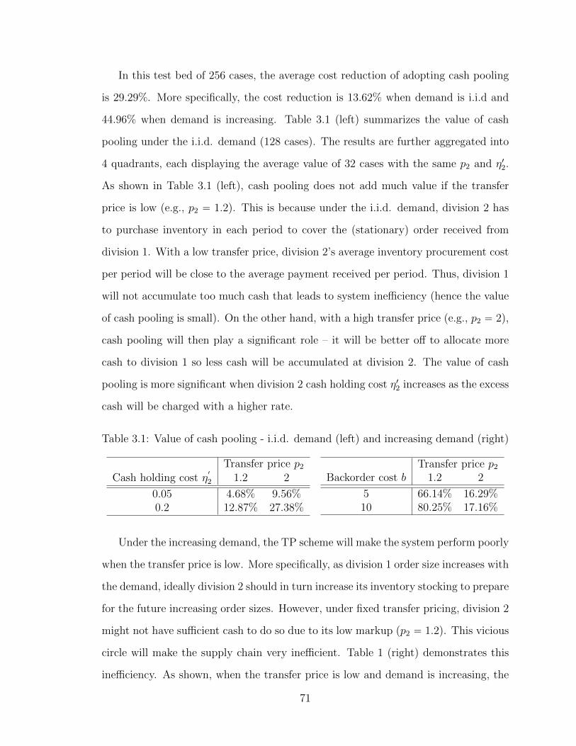
In this test bed of 256 cases, the average cost reduction of adopting cash pooling

is 29.29%. More specifically, the cost reduction is 13.62% when demand is i.i.d and

44.96% when demand is increasing. Table 3.1 (left) summarizes the value of cash

pooling under the i.i.d. demand (128 cases). The results are further aggregated into

4 quadrants, each displaying the average value of 32 cases with the same p2 and η12.

As shown in Table 3.1 (left), cash pooling does not add much value if the transfer

price is low (e.g., p2 “ 1.2). This is because under the i.i.d. demand, division 2 has

to purchase inventory in each period to cover the (stationary) order received from

division 1. With a low transfer price, division 2’s average inventory procurement cost

per period will be close to the average payment received per period. Thus, division 1

will not accumulate too much cash that leads to system inefficiency (hence the value

of cash pooling is small). On the other hand, with a high transfer price (e.g., p2 “ 2),

cash pooling will then play a significant role – it will be better off to allocate more

cash to division 1 so less cash will be accumulated at division 2. The value of cash

pooling is more significant when division 2 cash holding cost η12 increases as the excess

cash will be charged with a higher rate.

Table 3.1: Value of cash pooling - i.i.d. demand (left) and increasing demand (right)

Transfer price p2

Cash holding cost η1

2 1.2 2

0.05 4.68% 9.56%0.2 12.87% 27.38%

Transfer price p2

Backorder cost b 1.2 2

5 66.14% 16.29%10 80.25% 17.16%

Under the increasing demand, the TP scheme will make the system perform poorly

when the transfer price is low. More specifically, as division 1 order size increases with

the demand, ideally division 2 should in turn increase its inventory stocking to prepare

for the future increasing order sizes. However, under fixed transfer pricing, division 2

might not have sufficient cash to do so due to its low markup (p2 “ 1.2). This vicious

circle will make the supply chain very inefficient. Table 1 (right) demonstrates this

inefficiency. As shown, when the transfer price is low and demand is increasing, the

71

value of cash pooling can be very significant. Interestingly, this finding is consistent

with Caterpillar’s strategy: After the financial crisis, many suppliers of Caterpillar

have difficulty getting funds from external banks to stock up the raw material for the

expected soaring demand. Thus, Caterpillar took a more proactive role to subsidize

their suppliers (Aeppel, 2010). The value of cash pooling is clearly higher when

backorder cost is larger. Figure 3.7(a) summarizes the conditions under which cash

pooling has a significant value5.

Figure 3.7: Value of cash pooling

Figure 3.7(b) illustrates the impact of downstream liquidity level K on the value

of cash pooling when demand is increasing under different selling prices p1. Here, we

set the transfer price p2 “ 1.05, b “ 5, η1

2 “ 0.2, h1

2 “ 0.25, β1

o “ β1

i “ 0.05 and the

other parameters are the same as in the test bed. For a fixed selling price, the value

of cash pooling is increasing in K, but the marginal benefit of cash pooling decreases

in K. In addition, we find that p1 and K complement each other’s role as a liquidity

source. For example, pK, p1q “ p8, 1.2q and p4, 1.5q yield a similar CP value.

5 Figure 3.7(a) also shows that CR (SP) bound performs better in the upper left (lower right)quadrant.

72

3.5.2 Optimal Transfer Pricing

While we have demonstrated significant value of cash pooling, one interesting question

to investigate is that how much benefit can be recovered by optimizing the transfer

price. To answer this question, we compare the optimal cost from the CP model,

C˚, with the optimal cost from the OP model, CO. We define the percentage cost

reduction as pCO ´ C˚q{CO ˆ 100%. We test the same 256 instances. The average

(maximum, minimum) percentage cost reduction of adopting cash pooling is 6.38%

(9.98%, 3.34%) for the i.i.d. demand and 9.33% (14.75%, 4.65%) for the increasing

demand case. The cost reduction is more significant when the cash holding cost η1

2

or the backorder cost b is high. Two reasons lead to this cost difference. First, cash

pooling can consolidate the entire system cash to a single account that has a smaller

cash holding cost rate. (This explains why the cost saving is more significant when η21

is larger.) Second, cash pooling eliminates the lead time for the payment and allows

cash to move bi-directionally to upstream or downstream, making the supply chain

more responsive and leading to a smaller number of backorders. (Thus, the benefit

of cash pooling is more significant when the backorder cost is high.)

Compared with the cost reduction with the fixed transfer price tested in the

previous section, the percentage cost reduction is relatively small when the transfer

price is optimized. This suggests that optimizing the transfer price can retain a big

portion of the benefit achieved by adopting cash pooling. This indeed is useful for

firms if adopting cash pooling is not possible due to legal issues or cash shortage for

investing in the costly financial services platform.

It is interesting to see how the optimized transfer price helps to re-distribute the

supply chain cash between these two divisions for firms facing a product life cycle

demand. More specifically, we consider a time horizon of 22 periods with Poisson

demand in each period. The demand mean starts from 6, ramps up at a peak of

36, declines to 14 and remains there for the last 5 periods. These demand rates

73

represent introduction, growth, maturity, and decline stages in a product life cycle

(see Figure 3.8). To illustrate the transfer pricing dynamics, we consider a instance

with p2 “ 1.25, p1 “ 1.5, b “ 55, η12 “ 0.15, h12 “ 0.2, β1o “ β1i “ 0.05, K 1 “ 0, and the

other fixed parameters in the test bed. We obtain the optimal transfer price as the

optimal cash payment, m, divided by the optimal order quantity, z1 in a simulation

study and plot the average optimal transfer price in each period. Figure 3.9 shows the

dynamics of the corresponding optimal transfer price from period to period. Notice

that if the optimal transfer price p˚2 is larger than p1 “ 1.5, the price difference can

be viewed as financial subsidy offered by stage 1; on the other hand, if p˚2 is smaller

than the purchase cost c “ 1, the price difference can be viewed as delayed payment

made by stage 1.

Figure 3.8: Product life cycle demand

1 3 5 7 9 11 13 15 170

10

20

30

40

Time period

De

ma

nd

me

an

maturitygrowthintroduction decline

Figure 3.9: Optimal transfer price under product life cycle demand

1 3 5 7 9 11 13 15 170.5

1

1.5

2

Time period

Optim

al tr

ansfe

r price financial subsidy

payment delay

Figure 3.9 provides an interesting insight on how to set up the optimal transfer

price. Recall that this is a case with K 1 “ 0, i.e., the source of stage 1’s liquidity is

completely from the sales revenue. From the figure, we find that during the introduc-

tion stage, the transfer price should be set to a value close to the selling price p1. This

74

implies that division 1’s cash should be moved to division 2, as the latter needs to

spare more cash for material ordering. The transfer price declines slightly but ramps

up quickly during the growth stage, reflecting the fact that division 1 should even

subsidize division 2 for material ordering. Finally, during the maturity and decline

stages, division 2 does not need to reserve excess cash for material ordering, so the

transfer price declines gradually. During the periods 13 to 17, the transfer price can

be lower than the purchase cost c. We can view this as a payment reduction received

by division 1 to compensate the cash subsidy offered to division 2 during the growth

stage.

3.5.3 Bullwhip Effect

Bullwhip effect is a phenomenon that the order variability amplifies when moving

along the supply chain from downstream toward upstream stages (Lee et al., 1997).

It describes a phenomenon of order information distortion. In the empirical litera-

ture, material bullwhip effect, i.e., the amplification of shipments, is often used as

a proxy for the order bullwhip effect, and observed in practical supply chains (e.g.,

Blanchard, 1983; Cachon et al., 2007). Interestingly, in the finance literature, a simi-

lar phenomenon called “financial contagion” has been observed in practice (e.g., Allen

and Gale, 2000). The financial contagion describes that the risk of financial payment

defaults amplifies when moving toward upstream in a supply chain. One reason that

causes the financial contagion is the material bullwhip effect. This is because the pay-

ment amount is usually associated with the shipment size via transfer price. When

the shipment variability amplifies, an upstream stage requires more capital for its

inventory payments. If the upstream stage has weaker cash liquidity, which is usually

observed in supply chains, this will result in a higher payment default risk. In our

TP model, we observe that both material and financial bullwhip effect amplify in the

same direction with the same scale – in a simulation study based on the test bed of

the i.i.d. demand instances, we find that the average coefficient of variation (c.v.) of

75

the shipment received by (or the payment paid by) stage 1 and stage 2 is 0.28 and

0.32, respectively. Interestingly, by optimizing the transfer price, one can reverse the

direction of amplification for the payment variability. More specifically, for the OP

model with the same test bed, the average c.v. of the shipment received by stage 1

and stage 2 is 0.26 and 0.28, respectively, whereas the average c.v. of the payment

paid by stage 1 and stage 2 is 0.32 and 0.28, respectively. Our numerical finding

suggests that (1) the material and financial bullwhip effects may not amplify in the

same direction in an integrated supply chain, and (2) the optimal transfer pricing

is a useful tool to smoothen the payment variability to the outside vendor, which

mitigates the material bullwhip effect in the system.

3.6 Concluding Remarks

The paper studies the benefit of cash pooling for a corporation that owns a supply

chain with two divisions. We quantity the value of cash pooling by comparing two

cash management systems, representing different level of cash concentration. We

prove the exact optimal inventory and cash retention policy for the cash pooling

model and construct a lower bound to the optimal cost for the transfer pricing model.

We quantity the conditions under which investing in a financial services platform that

achieves cash pooling provides the most benefit. Our study suggests that monitoring

the entire supply chain working capital through an inter-departmental collaboration

between accounting and operations is crucial to ensure system efficiency. Our results

can be extended to the system with general lead times and number of stages, as well

as Markov modulated system parameters.

The focus of this paper is to derive a centralized solution for supply chains with

different cash management systems. This perspective is appropriate for a single-owner

supply chain. Nonetheless, there are decentralized supply chains in which the entities

are individual firms, each with its own interests. An important question for the

decentralized supply chain is to design an incentive scheme such that each individual

76

firm would choose the first best solution. The centralized solution we obtain can be

viewed as the first best solution for this purpose. We leave this decentralized control

issue for the future research.

77

4

Material Flow Variability

4.1 Introduction

We study the material bullwhip effect in supply chains, a phenomenon that the vari-

ability of shipment is amplified when moving upstream the supply chain. Economists

have observed this phenomenon in empirical studies. However, this observation ap-

pears to be counter-intuitive as they would expect the opposite - the “production

smoothing” effect (smaller shipment variability at the upstream stage). We provide

an analytical model to show that it is possible to observe both bullwhip and reverse

bullwhip effects in supply chains. These results can be extended to explain the ma-

terial bullwhip effect when inventory replenishment is subject to the cash constraint,

hence providing analytical support for the findings in Chapter 2 and Chapter 3.

4.2 Main Results

Let us consider a periodic-review, two-stage serial inventory system where stage 1

orders from stage 2, and stage 2 orders from an outside vendor with ample supply. The

system is subject to i.i.d. customer demand Dt and full backlog at both stages. The

optimal ordering policy for such a system is known static echelon base-stock policy,

78

from which an equivalent local base-stock policy can be derived (see Clark and Scarf

1960, Rosling 1989). Figure 4.1 shows the two-stage model with the material and

information flows in opposite directions. The material flow is composed of shipments

and sales, while the information flow includes orders and customer demand.

Figure 4.1: The two-stage supply chain model with material and information flows

Under the optimal local base-stock policy, it is clear that O2,t “ O1,t “ Dt´1.

Thus, we have varpO2,tq “ varpO1,tq “ varpDt´1q, i.e., the information flow has no

bullwhip effect.

Now let us examine the material flow in the two-stage supply chain. For this

purpose, we need to describe the shipment and sales in the system. We assume that

the lead time is one period for both stages. We formalize the sequence of events as

follows: At the beginning of the period, (1) both stages receive shipments released

in the last period; (2) both stages make an order decision; (3) inventory levels and

backorders at both stages are updated; During the period, demand occurs and sales

are realized; At the end of the period, all costs are calculated. We first describe the

notation. For stage j “ 1, 2 and period t, define

Mj,t “ shipment released to stage j from its upstream supplier

M0,t “ realized sales to the end customer

Oj,t “ order quantity from stage j to its upstream supplier

Bj,t “ local backorders after making the order decision

sj “ local base-stock level

Next, we express M2, M1 and M0 in terms of demand and local backorders, which

are in turn expressed in terms of demand and local base-stock levels. Note from the

79

system dynamic of stage 2, we have B2,t “ B2,t´1`Dt´1´M1,t, i.e., current period’s

backorder is the difference between the accumulated backorder B2,t´1`Dt´1 and the

released shipment M1,t. The dynamic of stage 1 is the same except that the realized

sales are shifted one period backwards, due to the zero information lead time from

stage 1 to the end customer. We summarize the results in the following lemma.

Lemma 1. For all t, we have M2,t “ Dt´1, and

M1,t “ B2,t´1 ´B2,t `Dt´1, (4.1)

M0,t´1 “ B1,t´1 ´B1,t `Dt´1, (4.2)

where the local backorders can be expressed as

B2,t “ ´mint0, s2 ´Dt´1u, (4.3)

B1,t “ ´mint0, s1 ´Dt´1 `mint0, s2 ´Dt´2uu. (4.4)

Remark Equation (4.2) presents the exact expression of sales in a multi-period

model with backorders. In inventory literature, however, an alternative expression

has been commonly used to approximate sales - the minimum of demand and on-

hand inventory. As shown here, this approximation is accurate only when B1,t´1 “ 0,

i.e., stage 1 has cleared its backlogs in period t´ 1.

Given Lemma 1, we define the material bullwhip ratio at stage 2 as varpM2,tq{varpM1,tq,

and that at stage 1 as varpM1,tq{varpM0,t´1q. The reverse material bullwhip occurs

whenever the material bullwhip ratio is less than 1.

Let us first consider the material flow from stage 2 to stage 1. Note from (4.3)

that when s2 ě 0, B2,t visits the zero point infinitely many times. Let us examine a

cycle that spans τ`1 periods between two consecutive zero-point visits, i.e., B2,t “ 0,

B2,t`1 ą 0, B2,t`2 ą 0, ..., B2,t`τ ą 0, and B2,t`τ`1 “ 0. In this cycle, the shipment

from stage 2 to stage 1 is given by

M1,t`i “

$

&

%

s2, if i “ 1,Dt`i´2, if 2 ď i ď τ,Dt`τ´1 `Dt`τ ´ s2, if i “ τ ` 1.

,

.

-

(4.5)

80

It turns out that we can show thatřτ`1i“1 M

22,tì “

řτ`1i“1 D

2tì´1 ě

řτ`1i“1 M

21,tì (see

the proof given in the appendix). Thus, the following proposition immediately follows

from the ergodic theorem.

Proposition 10. For any s2 ě 0, we have varpM2,tq “ varpDt´1q ě varpM1,tq.

Next, we consider the material flow from stage 1 to the end customer. We identify

the cycle in a similar way as in the proof of Proposition 10. When s1 ě 0, B1,t visits

the zero point infinitely many times. We examine a cycle that spans τ ` 1 periods

between two consecutive zero-point visits, i.e., B1,t “ 0, B1,t`1 ą 0, B1,t`2 ą 0, ...,

B1,t`τ ą 0, and B1,t`τ`1 “ 0. In this cycle, the sales from stage 1 to the customer

are given by

M0,tì´1 “

$

&

%

s1, if i “ 1,M1,tì´1, if 2 ď i ď τ,Dt`τ´1 `Dt`τ ´mint0, s2 ´Dt`τ´2u ´ s1, if i “ τ ` 1.

,

.

-

(4.6)

It turns out that we can leverage the above structure to show thatřτ`1i“1 M

21,tì ě

řτ`1i“1 M

20,tì´1 under the condition of s2 ě s1 (see the proof given in the appendix).

Again from the ergodic theorem we have the following proposition.

Proposition 11. For any s2 ě s1 ě 0, we have varpM1,tq ě varpM0,t´1q.

When s2 ă s1, the analysis becomes more complicated. And in fact, the rela-

tionship between varpM1,tq and varpM0,t´1q depends on s1, s2, and the demand. To

see this, we assume Dt follows a Uniform distribution with support r0, ds, denoted as

Up0, dq. Note that varpDtq “ d2{12. We first express varpM1,tq in terms of s2 and d.

Lemma 2. Assuming Dt follows Up0, dq, we have

varpM1,tq “

$

’

’

&

’

’

%

d2

12´s2

2

2

´

1´s2

d

¯2

, if s2 ď d,

d2

12, if s2 ą d.

,

/

/

.

/

/

-

(4.7)

81

Taking derivative of varpM1,tq with respect to s2 in the region of s2 ď d, we have

BvarpM1,tq

Bs2

“ ´s2

´

1´s2

d

¯

ˆ

1´2s2

d

˙

. (4.8)

Therefore, as s2 increases from 0 to d, varpM1,tq will first decrease then increase.

Figure 4.2 plots varpM1,tq as function of s2 when demand follows Up0, 12q. The

corresponding bullwhip ratio is plotted in Figure 4.3, which shows that the material

bullwhip effect at stage 2 is most significant when s2 “ d{2, with a bullwhip ratio of

1.6.

0 2 4 6 8 10 12 14 167

8

9

10

11

12

Va

ria

nce

of

sh

ipm

en

t

Stage 2 base−stock level

Figure 4.2: Variance of shipment varpM1,tq vs. base-stock s2 under Up0, 12q

0 2 4 6 8 10 12 14 161

1.2

1.4

1.6

1.8

Stage 2 base−stock level

Bu

llwh

ip r

atio

Figure 4.3: Bullwhip ratio varpM2,tq{varpM1,tq vs. base-stock s2 under Up0, 12q

Next, we derive varpM0,t´1q under uniformly distributed demand. Note that in

most supply chains, the unit backorder cost is usually much higher than the inventory

holding cost at the downstream stage. In our current model with one period lead time,

this indicates that the optimal base-stock s1 will be greater than d, the mean of the

sum of two independent uniformly distributed demand. Hence in what follows, we

focus on the case with d ă s1.

82

Lemma 3. Assuming Dt follows Up0, dq, we have

varpM0,t´1q “

$

’

’

’

&

’

’

’

%

d2{12, if d ă s2 ă s1,

d2{12, if s2 ď d ă s1 and 2d´ s2 ă s1,

d2

12´

1

2d

ż d

s1`s2´d

y2´

1´y

d

¯2

dy, if s2 ď d ď s1 ď 2d´ s2.

,

/

/

/

.

/

/

/

-

(4.9)

Now, we can combine Lemma 2 and Lemma 3 to compare varpM1,tq and varpM0,t´1q.

We discuss the results in three regions: (1) when d ă s2 ă s1, varpM2,tq “ varpM1,tq “

varpM0,t´1q, i.e., no material bullwhip at either stage; (2) when s2 ď d ă s1 and 2d´

s2 ă s1, varpM2,tq “ varpM0,t´1q ě varpM1,tq, i.e., bullwhip at stage 2 and reverse

bullwhip at stage 1; (3) when s2 ď d ď s1 ď 2d ´ s2, there is still bullwhip at stage

2, but the relationship between varpM1,tq and varpM0,t´1q could be either way. To

further explore this, let us define

varpM0,t´1q “d2

12´

1

2d

ż d

s2

y2´

1´y

d

¯2

dy, (4.10)

which is obtained from varpM0,t´1q by making s1 “ d. Note that varpM0,t´1q depends

on both s1 and s2, while varpM0,t´1q only depends on s2. Furthermore, it can be seen

from (4.10) that

varpM0,t´1qps2, s1q “ varpM0,t´1qps2 ` s1 ´ dq. (4.11)

It turns out that varpM0,t´1q can help us determine the threshold in comparing

varpM1,tq and varpM0,t´1q. As shown in Figure 4.4, threshold s2 is obtained as the in-

tersection of curve varpM1,tq and varpM0,t´1q. When s2 ă s2, there exists a threshold

s1ps2q that satisfies

s2 ` s1ps2q ´ d “ arg varpM0,t´1q pvarpM1,tqps2qq . (4.12)

It can be shown that varpM1,tq ě varpM0,t´1q if s1 ď s1, and the sign is flipped

otherwise. When s2 ą s2, varpM1,tq ă varpM0,t´1q for all s1. We formalize this result

in Proposition 12.

83

Figure 4.4: varpM1,tq and varpM0,t´1q as a function of base-stock s2 under Up0, 12q

Proposition 12. Assume Dt follows Up0, dq and consider the region R “ ts1, s2 |s2 ď

d ď s1 ď 2d´ s2u. Then, there exists a threshold s2 P p0, d{2q, such that for ps1, s2q P

R

1. When s2 ď s2, there exists a threshold s1 such that varpM1,tq ě varpM0,t´1q if

s1 ď s1, and varpM1,tq ă varpM0,t´1q if s1 ą s1;

2. When s2 ą s2, varpM1,tq ă varpM0,t´1q for all s1.

84

Appendix A

Proof of Results

A.1 Proof of Results in Chapter 2

Proposition 1.

Proof. We define πtpy, wq “ gtpyq ` αλppy´wq` and take the partial derivative with

respect to y:

B

Byπtpy, wq “

B

Bygtpyq `

"

0, if y ă wαλp, if w ă y

*

. (A.1)

Now, let us consider the three cases in the pd, Sq policy. For Case 1, i.e., w ď dt, it can

be shown from (2.15) that for small positive ε, B

Byπtpdt´ε, wq ă 0 and B

Byπtpdt`ε, wq ą

0. Since πtpy, wq is convex in y, we have y˚t pwq “ dt when w ď dt. The other two

cases can be similarly proved.

Lemma 1.

Proof. Taking the first derivative of gtpyq, we have

B

Bygtpyq “ ph` bqFtpyq ´ b` α

λp1´ αqcy. (A.2)

Then, the expressions in (2.17) can be obtained by solving B

Bygtpyq “ 0 and B

Bygtpyq “

´αλp.

85

Proposition 2.

Proof. (a) can be directly obtained from Lemma 1 and the definition of the usual

stochastic order. We prove (b) and (c) by induction. As shown in (2.11), the claim

trivially holds for t “ T ` 1. Assume Vt`1px,wq “ ´αλcx `Wt`1pwq for all px,wq P

Bt`1, then

Vtpx,wq “ ´αλcx`min

xďytJtpy, wqu , (A.3)

where Jtpy, wq “ Htpyq ` αλppy ´ wq` ` αλcy ` αEVt`1py ´ Dt, w ` θDtq. To solve

the problem in (A.3), we consider the following three cases.

Case 1: wt ď dt. To see that dt is a minimizer of Jt, note from (a) and demand

non-negativity that xt`1 “ dt ´ Dt ď dt`1, i.e., pxt`1, wt`1q P Bt`1. From induction

and Proposition 1, it can be shown that y˚t pwtq “ dt. If xt ď dt, i.e., pxt, wtq P Bt, the

base-stock is achievable, then

Wtpwtq “ minxtďy

tJtpy, wtqu “ αEWt`1pwt ` θDtq ` Ltpwtq.

Case 2: dt ă wt ď St. To see that wt is a minimizer of Jt, note from (a) and demand

non-negativity that xt`1 “ wt ´ Dt ď St ď St`1 and xt`1 “ wt ´ Dt ď wt ` θDt “

wt`1. Therefore, xt`1 ď St`1 ^ wt`1, i.e., pxt`1, wt`1q P Bt`1. From induction and

Proposition 1, it can be shown that y˚t pwtq “ wt. If xt ď wt, i.e., pxt, wtq P Bt, the


Wtpwtq “ minxtďy

tJtpy, wtqu “ αEWt`1pwt ` θDtq ` gtpwtq.

Case 3: St ă wt. To see that St is a minimizer of Jt, note from (a) and demand

non-negativity that xt`1 “ St ´ Dt ď St`1 and xt`1 “ St ´ Dt ă wt ` θDt “

wt`1. Therefore, xt`1 ď St`1 ^ wt`1, i.e., pxt`1, wt`1q P Bt`1. From induction and

Proposition 1, it can be shown that y˚t pwtq “ St. If xt ď St, i.e., pxt, wtq P Bt, the


Wtpwtq “ minxtďy

tJtpy, wtqu “ αEWt`1pwt ` θDtq ` gtpStq.

86

Summarizing the above three cases, we prove the optimality of the pd, Sq policy

and the decomposition of Vtpx,wq. Moreover, since Wt`1p¨q is convex from induction,

Wtp¨q is also convex.

Lemma 2.

Proof. From (2.22) and (2.25), M´puq ďMpuq can be directly obtained by applying

Jensen’s inequality. Furthermore, when uÑ 8, M´puq “Mpuq “ ppu´ ρµmq.

Lemma 3.

Proof. Lemma 2 shows that M´puq ďMpuq for all u. From the construction of Γpuq

and convexity of Mpuq, we have Γpuq ď Mpuq. Then from (2.26), Mpuq ď Mpuq

holds for all u. Now, we replace Mt with M´t and prove the result by induction. Let

V ´t px,wq be the minimum expected cost function by replacing Mt with M´t . It can

be easily shown that V ´T`1px,wq “ VT`1px,wq. Assume V ´t`1px,wq ď Vt`1px,wq for

all px,wq, then

V ´t px,wq “ minxďy

Htpyq ` αmM´

t py ´ wq ` αmcpy ´ xq ` αEV ´t`1py ´Dt, w ` θDtq

(

ď minxďy

tHtpyq ` αmMtpy ´ wq ` α

mcpy ´ xq ` αEVt`1py ´Dt, w ` θDtqu

“ Vtpx,wq.

Similar proof applies to the statement with Mt.

Lemma 4. The proof is straightforward algebra and hence omitted here.

Proposition 3.

Proof. We define πtpy, wq “ gtpyq ` αmMtpy ´ w ` ρµmt q and take derivative with

respect to y:

B

Byπtpy, wq “

B

Bygtpyq `

$

&

%

0, if y ă w ´ a1tαmpt, if w ´ a1t ă y ă w ` a2tαmp, if w ` a2t ă y

,

.

-

. (A.4)

87

Now, let us consider the five cases in the pd, a, Sq policy. For Case 1, i.e., w ď

dt ´ a2t , it can be shown from (2.35) that for small positive ε, B

Byπtpdt ´ ε, wq ă 0

and B

Byπtpdt ` ε, wq ą 0. Since πtpy, wq is convex in y, we have y˚t pwq “ dt when

w ď dt ´ a2t . The proofs of other cases are similar.

Lemma 5.

Proof. Same as the proof of Lemma 1 by replacing gtp¨q with gtp¨q, and ´αλp with

´αmpt.

Proposition 4.

Proof. (a) can be directly obtained from Lemma 1, Lemma 5, and the definition of

the usual stochastic order. We now prove (b) and (c) by induction. First, we derive

y˚pwq from (2.33) and the definition of w as follows:

y˚pwq “

$

’

’

’

’

&

’

’

’

’

%

d, if w ` ρA2 ď dw ` ρA2, if d ă w ` ρA2 ď dd, if w ` ρA1 ď d ă w ` ρA2

w ` ρA1, if d ă w ` ρA1 ď SS, if S ă w ` ρA1

,

/

/

/

/

.

/

/

/

/

-

. (A.5)

Thus, xt ď y˚t pwtq is equivalent to xt ď y˚t pwtq, i.e., pxt, wtq P Bt. As shown in (2.32),

the claim trivially holds for t “ T ` 1. Assume Vt`1px, wq “ ´αmcx ` Wt`1pwq for

all px, wq P Bt`1, then

Vtpx, wq “ ´αmcx`min

xďy

Jtpy, wq(

, (A.6)

where Jtpy, wq “ Htpyq ` αmMtpy ´ w ` ρµmt q ` αmcy ` αEVt`1py ´ Dt, w ` θDt `

ρµt`m ´ ρµtq. To solve the problem in (A.6), we consider the following five cases.

Case 1: wt ď dt ´ a2t , i.e., wt ` ρA2t ď dt. To see that dt is a minimizer of Jt,

note from (a) and demand non-negativity that xt`1 “ dt ´Dt ď dt`1. Therefore, we

have pxt`1, wt`1q P Bt`1. From induction and Proposition 3, it can be shown that

y˚t pwtq “ dt. If xt ď dt, i.e., pxt, wtq P Bt, the base-stock is achievable, the rest of the

proof is similar to Proposition 2.

88

Case 2: dt ´ a2t ă wt ď dt ´ a2t , i.e., dt ă wt ` ρA2t ď dt. To see that wt ` a2t is a

minimizer of Jt, note from (a) and demand non-negativity that xt`1 “ wt`ρA2t´Dt ď

dt`1 and xt`1 “ wt` ρA2t ´Dt ď wt` θDt` ρA

2t ď wt`1` ρA

2t`1. Therefore, we have

pxt`1, wt`1q P Bt`1. The rest of the proof is similar to Case 1.

Case 3: dt ´ a2t ă wt ď dt ` a1t, i.e., wt ` ρA1t ď dt ă wt ` ρA2t . To see that dt is

a minimizer of Jt, note from (a) and demand non-negativity that xt`1 “ dt ´ Dt ď

dt`1 and xt`1 “ dt ´ Dt ă wt ` θDt ` ρA2t ď wt`1 ` ρA2t`1. Therefore, we have


Case 4: dt ` a1t ă wt ď St ` a1t, i.e., dt ă wt ` ρA1t ď St. To see that wt ´ a1t is a

minimizer of Jt, note from (a) and demand non-negativity that xt`1 “ wt`ρA1t´Dt ď

St`1 and xt`1 “ wt` ρA1t´Dt ď wt` θDt` ρA

1t ď wt`1` ρA

1t`1. Therefore, we have


Case 5: St ` a1t ă wt, i.e., St ă wt ` ρA1t. To see that St is a minimizer of Jt, note

from (a) and demand non-negativity that xt`1 “ St´Dt ď St`1 and xt`1 “ St´Dt ď

wt` θDt`ρA1t ď wt`1`ρA

1t`1. Therefore, from (A.5) we have xt`1 ď y˚t pwt`1q, thus,


Summarizing the above three cases, we prove the optimality of the pd, a, Sq policy

and the decomposition of Vtpx, wq. Since Wt`1p¨q is convex from induction, Wtp¨q is

also convex.

Lemma 6.

Proof. To simplify the notation, we assume m “ 1 and drop the superscript without

loss of generalization. By definition of loss function, we have

Ftpµtq “

ż 8

µt

Ftpyqdy “

ż µt

0

Ftpyqdy “

ż Ftpµtq

0

pµt ´ F´1t pyqqdy,

89

where F´1p¨q is the inverse function of F p¨q. From (2.27) we have

A1t “ pµtFtpµtq ´ Ftpµtqq{Ftpµtq “

ż Ftpµtq

0

F´1t pyqdy{Ftpµtq.

Similarly, it can be shown that A2t “ş1

FtpµtqF´1t pyqdy{Ftpµtq. Due to usual stochastic

order, F´1t pyq is increasing in t for any y P r0, 1s. Given that At “ Ftpµtq “ 1´ Ftpµtq

is constant over t, we have A1t and A2t are increasing in t.

Proposition 5. Similar to the proof of Proposition 2 and hence omitted here.


Lemma 9 (Karush, 1959) shows the additive separation of a function value.

Lemma 9. If a function fpyq is convex on p´8,8q and attains its minimum at y˚,

then

minaďyďb

fpyq “ fLpaq ` fUpbq,

where fLpaq “ minaďy fpyq is convex non-decreasing in a, and fUpbq “ fpbq´fpb_y˚q

is convex non-increasing in b.

Proposition 6.

Proof. We prove by induction. The claim trivially holds for t “ T ` 1. Assume

Vt`1px, wq “ f1,t`1px1q ` f2,t`1px2q ` f3,t`1pwq, then

Vtpx, wq “ miny,rPSpx,wq

$

&

%

H1,tpx1q ` αEDtf1,t`1py1 ´Dtq

`H2,tpx2q ` cpy2 ´ x2q ` αEDtf2,t`1py2 ´Dtq

`H3,tprq ` βipr ´ wq` ` βopr ´ wq

´ ` αEDtf3,t`1pr ` θDtq

,

.

-

.

(A.7)

Let g1,tpy1q “ αEDtf1,t`1py1 ´ Dtq, and g2,tpy2q “ cy2 ` αEDtf2,t`1py2 ´ Dtq. Since

fi,t`1p¨q is convex (from induction), by Lemma 9 we can decompose the cost functions:

minx1ďy1ďx2

g1,tpy1q “ minx1ďy1


` Γ2,tpx2q,

minx2ďy2ďr

g2,tpy2q “ minx2ďy2

cy2 ` αEDtf2,t`1py2 ´Dtq(

` Γ3,tprq,

90

where the induced penalty functions Γ2,tpx2q and Γ3,tprq are expressed in (3.12) and

(3.13), respectively.

Now, let us define f1,tpx1q as in (3.9), and

g3,tprq “ H3,tprq ` Γ3,tprq ` αEDtf3,t`1pr ` θDtq.

Plugging the expressions of f1,tpx1q and g3,tprq in (A.7), we have

Vtpx, wq “ f1,tpx1q `H2,tpx2q ` Γ2,tpx2q ` minx2ďy2


` minx2ďrďw`K

g3,tprq ` βipr ´ wq`` βopr ´ wq

´(

. (A.8)

Let rt “ arg minr

g3,tprq(

, and r˚t “ arg minr

g3,tprq` βipr´wq`` βopr´wq

´(

.

The convexity of g3,tprq implies the existence of the one-sided derivative Bg3,tprq{Br.

Define

l˚t “ suptr :Bg3,tprq

Brď ´βiu, u˚t “ suptr :

Bg3,tprq

Brď βou.

The monotonicity of Bg3,tprq{Br implies l˚t ď rt ď u˚t . Using Proposition B-7 in

Heyman and Sobel (1984), we have

r˚t “

$

&

%

l˚t , if w ď l˚t ,w, if l˚t ă w ď u˚t ,u˚t , if u˚t ă w.

,

.

-

(A.9)

Define Ltpwq “ ´βipw ´ l˚t q ` g3,tpl

˚t q, Utpwq “ βopw ´ u

˚t q ` g3,tpu

˚t q, and let

Wtpwq “

$

&

%

Ltpwq, if w ď l˚t ,g3,tpwq, if l˚t ă w ď u˚t ,Utpwq, if u˚t ă w.

,

.

-

(A.10)

From (A.9) it can be easily shown that

Wtpwq “ minrtg3,tprq ` βipr ´ wq

`` βopr ´ wq

´u.

Now, we impose the constraint x2 ď r ď w `K. First, let

r˚˚t “ arg minx2ďrďw`K


´(

, (A.11)

91

and define the induced penalty functions Λ2,tpx2q and Λ3,tpwq according to (3.17) and

(3.18), respectively. Then, we define f3,tpwq as in (3.11). The convexity of f3,tpw1q

can be easily proved by showing that Bf3,tpwq{Bw is non-decreasing in w. Next, we

prove the decomposition of echelon 3:

minx2ďrďw`K


´(

“ f3,tpwq ` Λ2,tpx2q. (A.12)

The echelon system dynamics and constraint guarantee that x2 ď w holds for all

periods. To prove (A.12), we consider all possible relationships between x2, w, l˚t and

u˚t , as extensively described in the four cases below.

Case 1. When w ď l˚t ´K, we have r˚˚t “ w`K ď l˚t , f3,tpwq “ g3,tpw`Kq ` βiK,

and Λ2,tpx2q “ 0. Thus, f3,tpwq ` Λ2,tpx2q “ g3,tpw `Kq ` βiK “ g3,tpr˚˚t q ` βipr

˚˚t ´

wq` ` βopr˚˚t ´ wq´, i.e., (A.12) holds.

Case 2. When l˚t ´ K ă w ď l˚t , we have r˚˚t “ r˚t “ l˚t , f3,tpwq “ Ltpwq and

Λ2,tpx2q “ 0. Clearly, (A.12) holds.

Case 3. When l˚t ă w, and x2 ď u˚t , we have r˚˚t “ r˚t “ rt, f3,tpwq “ g3,tpwq, and

Λ2,tpx2q “ 0. Clearly, (A.12) holds.

Case 4. When u˚t ă x2 ď w, we have r˚˚t “ x2, f3,tpwq “ Utpwq and Λ2,tpx2q “

g3,tpx2q ´ Utpx2q. Thus, f3,tpwq ` Λ2,tpx2q “ g3,tpx2q ` Utpwq ´ Utpx2q “ g3,tpx2q `

βipw ´ x2q “ g3,tpr˚˚t q ` βipr

˚˚t ´ wq` ` βopr

˚˚t ´ wq´, i.e., (A.12) holds.

Therefore, we verified that (A.12) holds in all cases. Substituting (A.12) into (A.8),

and defining f2,tpx2q as in (3.10), we complete the induction Vtpx, wq “ f1,tpx1q `

f2,tpx2q ` f3,tpwq. Using Lemma 9, all induced penalty functions are convex, thus,

fi,tp¨q is convex, pi “ 1, 2, 3q.

Proposition 7.

Proof. We prove by induction. VT`1px,wq “ 0 “ V 1T`1px1, w1q ` V 2

T`1px1, x2, w2q.

92

Suppose Vt`1px,wq ě V 1t`1px1, w1q ` V

2t`1px1, x2, w2q for all px,wq, then

Vtpx,wq “ miny,r1PSpx,wq

tGtpx,w, y2, r1q (A.13)

`αEDtVt`1py1 ´Dt, y2 ´Dt, w2 ` ρpy1 ´ x1q ´Dt, r1 ` θDtqu

ě miny,r1PSpx,wq

tGtpx,w, y2, r1q (A.14)

`αEDtV1t`1py1 ´Dt, r1 ` θDtq ` αEDtV

2t`1py1 ´Dt, y2 ´Dt, w2 ` ρpy1 ´ x1q ´Dtq

(

ě miny,r1PSpx,wq



(

(A.15)

` miny,r1PSpx,wq

G2t px, w2, y2q ` αEDtV


(

ě minx1ďy1ďr1ďw1`K



(

(A.16)

` minx1ďy1ďx2ďy2ďw2

G2t px, w2, y2q ` αEDtV


(

“ V 1t px1, w1q ` V

2t px1, x2, w2q. (A.17)

The inequality in (A.14) and (A.16) are due to induction and constraint relaxation,

respectively. The above relationship holds for all px,wq in period t, completing the

induction.

Lemma 7.

Proof. We write out the flow conservation of w2 and x1 from s “ 1 to s “ t´ 1.

ED1,...,Dt´1

w2,t ´ w2,1 “ÿt´1

s“1ρz1,s ´

ÿt´1

s“1µs, (A.18)

ED1,...,Dt´1

x1,t ´ x1,1 “ÿt´1

s“1z1,s ´

ÿt´1

s“1µs. (A.19)

The result is shown by subtracting ρˆ(A.19) from (A.18).

Proposition 8.

Proof. We first specify the cost functions when demand is deterministic. Define

H2d1,tpx1q “ ph

21 ` h2 ` η2 ` b2qpdtpωq ´ x1q

`` h2

1px1 ´ dtpωqq,

Hd2,tpx2q “ h2px2 ´ dtpωqq, Hd

3,tpaq “ η2pa´ dtpωqq.

93

We then prove by induction. The claim trivially holds for t “ T `1. Now, we assume

V dt`1px1, x2 | ωq “ v1

t`1px1 | ωq ` v2t`1px2 | ωq. Let gd1,t “ αvit`1py1 ´ dpωq | ωq and

gd2,t “ c2y2 ` αvit`1py2 ´ dpωq | ωq. From the convexity of vit`1p¨q and Lemma 9, we

can decompose the cost functions of echelon 1 and 2 as follows:

minx1ďy1ďx2

gd1,tpy1q “ minx1ďy1

αv1t`1py1 ´ dpωq | ωq

(

` Γd2,tpx2q,

minx2ďy2ďa

gd2,tpy2q “ minx2ďy2

cy2 ` αv2t`1py2 ´ dpωq | ωq

(

` Γd1,tpaq,

where a “ ρx1 `Btpωq. Let y˚1,t minimize gdi,tpyiq, the induced penalty functions are

Γd2,tpx2q “

"

α“

v1t`1px2 ´ dtpωq | ωq ´ v

1t`1py

˚1,t ´ dtpωq | ωq

‰

, x2 ď y˚1,t,0, otherwise,

*

Γd1,tpx1q “

"

cpa´ y˚2,tq ` α“

v2t`1pa´ dtpωq | ωq ´ v

2t`1py

˚2,t ´ dtpωq | ωq

‰

, a ď y˚2,t,0, otherwise.

*

From Lemma 9, the functions above are convex. Therefore, the following functions

are convex:

v1t px1 | ωq “ H2d

1,tpx1q `Hd3,tpaq ` Γd1,tpaq ` min

x1ďy1

αv1t`1py1 ´ dtpωq | ωq

(

,

v2t px2 | ωq “ Hd

2,tpx2q ` Γd2,tpx2q ` minx2ďy2

cpy2 ´ x2q ` αv2t`1py2 ´ dtpωq | ωq

(

.

Furthermore, V dt px1, x2 | ωq “ v1

t px1 | ωq ` v2t px2 | ωq, completing the proof.


Lemma 1.

Proof. Since stage 2 orders from an ample supply, it can be easily shown that M2,t “

Dt´1. Equation (4.1) and (4.2) can be directly obtained from the system dynamics

B2,t “ B2,t´1`Dt´1´M1,t, and B1,t “ B1,t´1`Dt´1´M0,t´1, respectively. To derive

local backorders B2,t and B1,t, we need the dynamics of local net inventory levels. For

stage j “ 1, 2 and period t, define

ILj,t “ local net inventory level after receiving the shipment

“ sj ´Dt´1 ´Bj`1,t´1

94

where B3,t ” 0 due to the ample supply. Plugging the above relationship into Bj,t “

´mint0, ILj,tu, we can immediately get equation (4.3) and (4.4). Below we write out

the full expressions of M1,t and M0,t´1 for future reference.

M1,t “mint0, s2 ´Dt´1u ´mint0, s2 ´Dt´2u `Dt´1, (A.20)

M0,t´1 “mint0, s1 ´Dt´1 `mint0, s2 ´Dt´2uu

´mint0, s1 ´Dt´2 `mint0, s2 ´Dt´3uu `Dt´1, (A.21)

completing the proof.

Proposition 10.

Proof. For any cycle such that B2,t “ 0, B2,t`1 ą 0, B2,t`2 ą 0, ..., B2,t`τ ą 0,

B2,t`τ`1 “ 0, we have Dt´1 ď s2, Dt ą s2, Dt`1 ą s2, ..., Dt`τ´1 ą s2, Dt`τ ď s2.

Recall from Lemma 1 that M2,t “ Dt´1. Applying (A.20) repeatedly, we have

τ`1ÿ

i“1

M22,tì ´

τ`1ÿ

i“1

M21,tì

“

τ`1ÿ

i“1

D2tì´1 ´

«

s22 `

τ´1ÿ

i“1

D2tì´1 ` pDt`τ´1 `Dt`τ ´ s2q

2

ff

“ 2s2Dt`τ´1 ` 2s2Dt`τ ´ 2Dt`τ´1Dt`τ ´ 2s22

“ 2pDt`τ´1 ´ s2qps2 ´Dt`τ q ě 0.

Thus, we conclude thatřτ`1i“1 M

22,tì ě

řτ`1i“1 M

21,tì. Note that M1,t “ Dt´1 “ M2,t

when B2,t´1 “ B2,t “ 0, i.e., when period t is not included in any cycle. Also,

it is straightforward to verify thatřτ`1i“1 M2,tì “

řτ`1i“1 M1,tì. Because B2,t is a

stationary process, by the ergodic theorem, we conclude that ErM22,ts ě ErM2

1,ts and

ErM2,ts “ ErM1,ts. Therefore, varpM2,tq ě varpM1,tq, completing the proof.

Proposition 11.

Proof. For any cycle such that B1,t “ 0, B1,t`1 ą 0, B1,t`2 ą 0, ..., B1,t`τ ą 0,

B1,t`τ`1 “ 0, we calculate M0,tì´1 for i “ 1, ..., τ ` 1 in the following three steps.

95

(a) For i “ 1, since B1,t “ 0 and B1,t`1 ą 0, we have Dt´1 ď s1 ` mint0, s2 ´

Dt´2u ď s1 ď s2, hence, M0,t “ s1 `mint0, s2 ´Dt´1u “ s1.

(b) For i “ 2, ..., τ , since B1,tì´1 ą 0 and B1,tì ą 0, we have M0,tì´1 “

mint0, s2 ´Dtì´2u ´mint0, s2 ´Dtì´3u `Dtì´2 “M1,tì´1.

(c) For i “ τ`1, since B1,t`τ ą 0 and B1.t`τ`1 “ 0, we haveDt`τ ď s1`mint0, s2´

Dt`τ´1u ď s1 ď s2, and M0,t`τ “ Dt`τ´1 `Dt`τ ´mint0, s2 ´Dt`τ´2u ´ s1.

Combining results (a) and (b), we have

τ`1ÿ

i“1

M21,tì ´

τ`1ÿ

i“1

M20,tì´1 “M2

1,t`τ `M21,t`τ`1 ´

“

s21 `M

20,t`τ

‰

, (A.22)

where from Lemma 1 and result (c) above, we have

M1,t`τ “ mint0, s2 ´Dt`τ´1u ´mint0, s2 ´Dt`τ´2u `Dt`τ´1,

M1,t`τ`1 “ Dt`τ ´mint0, s2 ´Dt`τ´1u,

M0,t`τ “ Dt`τ´1 `Dt`τ ´mint0, s2 ´Dt`τ´2u ´ s1.

As shown above, it is not immediately clear whether M1,t is more variable than

M0,t´1. To further simplify (A.22), we discuss the following four cases.

Case 1. When Dt`τ´2 ď s2 and Dt`τ´1 ď s2, from B1,t`τ ą 0 we have Dt`τ´1 ą

s1 ` mint0, s2 ´ Dt`τ´2u “ s1. Together with Dt`τ ď s1 as in result (c), equation

(A.22) becomes

τ`1ÿ

i“1

M21,tì ´

τ`1ÿ

i“1

M20,tì´1 “ D2

t`τ´1 `D2t`τ ´

“

s21 ` pDt`τ´1 `Dt`τ ´ s1q

2‰

“ 2pDt`τ´1 ´ s1qps1 ´Dt`τ q ě 0.

Case 2. When Dt`τ´2 ď s2 and Dt`τ´1 ą s2, from B1.t`τ`1 “ 0 we have Dt`τ ď

s1 `mint0, s2 ´Dt`τ´1u “ s1 ` s2 ´Dt`τ´1. Therefore, equation (A.22) becomes

τ`1ÿ

i“1

M21,tì ´

τ`1ÿ

i“1

M20,tì´1 “ s2

2 ` pDt`τ´1 `Dt`τ ´ s2q2´“

s21 ` pDt`τ´1 `Dt`τ ´ s1q

2‰

“ 2ps2 ´ s1qps2 ` s1 ´Dt`τ´1 ´Dt`τ q ě 0.

96

Case 3. When Dt`τ´2 ą s2 and Dt`τ´1 ď s2, from B1,t`τ ą 0 we have Dt`τ´1 `

Dt`τ´2 ą s1 ` s2. Together with Dt`τ ď s1 as in result (c), equation (A.22) becomes

τ`1ÿ

i“1

M21,tì ´

τ`1ÿ

i“1

M20,tì´1 “ pDt`τ´2 `Dt`τ´1 ´ s2q

2`D2

t`τ

´“

s21 ` pDt`τ´2 `Dt`τ´1 `Dt`τ ´ s2 ´ s1q

2‰

“ 2ps1 ´Dt`τ qpDt`τ´2 `Dt`τ´1 ´ s2 ´ s1q ě 0.

Case 4. When Dt`τ´2 ą s2 and Dt`τ´1 ą s2, from B1.t`τ`1 “ 0 we have Dt`τ ď

s1`mint0, s2´Dt`τ´1u “ s1`s2´Dt`τ´1. Together with Dt`τ´2 ą s2 ě s1, equation

(A.22) becomes

τ`1ÿ

i“1

M21,tì ´

τ`1ÿ

i“1

M20,tì´1 “ D2

t`τ´2 ` pDt`τ´1 `Dt`τ ´ s2q2

´“

s21 ` pDt`τ´2 `Dt`τ´1 `Dt`τ ´ s2 ´ s1q

2‰

“ 2pDt`τ´2 ´ s1qps2 ` s1 ´Dt`τ´1 ´Dt`τ q ě 0.

Since the above four cases include all possible demand sample paths, we can

conclude thatřτ`1i“1 M

21,tì ě

řτ`1i“1 M

20,tì´1. Note that when B1,t´1 “ B1,t “ 0, we

have Dt´1 ď s1 ď s2 and Dt´2 ď s1 ď s2. Hence M1,t “M0,t´1 “ Dt´1 when period t

is not included in any cycle. Also, it is straightforward to verify thatřτ`1i“1 M1,tì “

řτ`1i“1 M0,tì´1. Because B1,t is a stationary process, by the ergodic theorem, we

conclude that ErM21,ts ě ErM2

0,t´1s and ErM1,ts “ ErM0,t´1s. Therefore, varpM1,tq ě

varpM0,t´1q, completing the proof.

Lemma 2.

Proof. The proof is trivial when s2 ą d. We derive varpM1,tq when s2 ď d. From

(A.20) we have

M1,t “ mint0, s2 ´Dt´1u ´mint0, s2 ´Dt´2u `Dt´1

“ mints2, Dt´1u `maxts2, Dt´2u ´ s2.

97

Let X “ mints2, Dt´1u. Since Dt follows Up0, dq, we have

EpXq “1

d

ż s2

0

xdx`1

d

ż d

s2

s2dx “ s2 ´s2

2

2d, (A.23)

EpX2q “

1

d

ż s2

0

x2dx`1

d

ż d

s2

s22dx “ s2

2 ´2s3

2

3d, (A.24)

Similarly, define Y “ maxts2, Dt´2u, and we have

EpY q “1

d

ż s2

0

s2dx`1

d

ż d

s2

xdx “d

2`s2

2

2d, (A.25)

EpY 2q “

1

d

ż s2

0

s22dx`

1

d

ż d

s2

x2dx “d2

3`

2s32

3d. (A.26)

Since X and Y are independent, we have

varpM1,tq “ varpXq ` varpY q

“ EpX2q ´ rEpXqs2 ` EpY 2

q ´ rEpY qs2

“s3

2

3d´

s42

4d2`

ˆ

2s32

3d´

s42

4d2`d2

12´s2

2

2

˙

“d2

12´s2

2

2

´

1´s2

d

¯2

, (A.27)

completing the proof.

Lemma 3.

Proof. The proof is trivial when d ă s2 ă s1. We derive varpM0,t´1q for the other two

cases. First, when s2 ď d ă s1 and 2d´ s2 ă s1, from (A.21) we have

M0,t´1 “ mints2, Dt´2, Dt´2 `Dt´1 ´ s1u `maxts2, Dt´3, s1 ` s2 ´Dt´2u ´ s2

(A.28)

“ mints2, Dt´2 `Dt´1 ´ s1u `maxtDt´3, s1 ` s2 ´Dt´2u ´ s2 (A.29)

“ Dt´1, (A.30)

where (A.28) is simple algebra, (A.29) is due to d ă s1, and (A.30) is due to 2d´s2 ă

s1. Therefore, varpM0,t´1q “ varpDt´1q “ d2{12.

98

Next, we show the case s2 ď d ď s1 ď 2d´ s2. Let us rewrite (A.29) as

M0,t´1 “ mints1 ` s2 ´Dt´2, Dt´1u `maxts1 ` s2 ´Dt´2, Dt´3u `Dt´2 ´ s1 ´ s2.(A.31)

Let Dt´2 “ x. When x ď s1 ` s2 ´ d, i.e., s1 ` s2 ´ x ě d, we have

EpM0,t´1 | xq “ EpDt´1 | xq “ EpDt´1q “ d{2,

varpM0,t´1 | xq “ varpDt´1 | xq “ varpDt´1q “ d2{12.

When x ą s1` s2´ d, replacing s2 with s1` s2´ x in (A.23), (A.25), and (A.27), we

have

EpM0,t´1 | xq “ s1 ` s2 ´ x´ps1 ` s2 ´ xq

2

2d`

ˆ

d

2`ps1 ` s2 ´ xq

2

2d

˙

` x´ s1 ´ s2 “d

2,

varpM0,t´1 | xq “d2

12´ps1 ` s2 ´ xq

2

2

´

1´s1 ` s2 ´ x

d

¯2

.

Therefore, varpEpM0,t´1 | xqq “ 0. Denoting y “ s1 ` s2 ´ x, we have

varpM0,t´1q “ 0` ExpvarpM0,t´1 | xqq

“1

d

ż s1`s2´d

0

d2

12dx`

1

d

ż d

s1`s2´d

„

d2

12´ps1 ` s2 ´ xq

2

2

´

1´s1 ` s2 ´ x

d

¯2

dx

“d2

12´

1

2d

ż d

s1`s2´d

y2´

1´y

d

¯2

dy.

Proposition 12.

Proof. Solving the integration in (4.10), we have

varpM0,t´1q “d2

15`s3

2

6d´

s42

4d2`

s52

10d3. (A.32)

Taking derivative of varpM0,t´1q with respect to s2, we have

BvarpM0,t´1q

Bs2

“s2

2

2d

´

1´s2

d

¯2

ě 0, (A.33)

99

i.e., varpM0,t´1q is increasing throughout r0, ds.

Now, let us first examine s2 P r0, d{2s, in which varpM1,tq is decreasing according

to (4.8). Moreover, it can be verified that varpM1,tq ă varpM0,t´1q when s2 “ 0, and

varpM1,tq ą varpM0,t´1q when s2 “ d{2. Therefore, there exists a point s2 P p0, d{2q

such that

varpM1,tqps2q “ varpM0,t´1qps2q.

Next, we examine s2 P pd{2, ds. Note that for any y ą s2 P pd{2, dq, we have

y2p1´ y{dq2 ă s22p1´ s2{dq

2. Therefore from (4.10) we have for any s2 P pd{2, dq

varpM0,t´1q ąd2

12´

1

2pd´ s2q

ż d

s2

s22

´

1´s2

d

¯2

dy “ varpM1,tq.

In addition, varpM0,t´1q “ varpM1,tq when s2 “ d. Thus, varpM1,tq ă varpM0,t´1q if

s2 P r0, d{2q, and the sign is flipped if s2 P pd{2, dq. Then, the results can be verified

using (4.11) and the continuity of varpM0,t´1q and varpM1,tq.

100

Bibliography

Abdallah, W. 1989. International transfer pricing policies: Decision-making guidelinesfor multinational companies. Praeger Santa Barbara, California.

Aeppel, T. 2010. Bullwhip hits firms as growth snaps back. Wall Street JournalJanuary 27.

Allen, F., D. Gale. 2000. Financial contagion. The Journal of Political Economy108(1) 1–33.

Angelus, A. 2011. A multiechelon inventory problem with secondary market sales.Management Science Forthcoming.

Angelus, A., E. L. Porteus. 2002. Simultaneous capacity and production managementof short-life-cycle, produce-to-stock goods under stochastic demand. ManagementScience 48(3) 399–413.

Babich, V. 2010. Independence of capacity ordering and financial subsidies to riskysuppliers. Manufacturing & Service Operations Management Service OperationsManagement 12(4) 583–607.

Babich, V., M. Sobel. 2004. Pre-ipo operational and financial decisions. ManagementScience 50(7) 935–948.

Baumol, W. 1952. The transaction demand for cash: An inventory theoretic approach.Quarterly Journal of Economics 66(4) 545–556.

Bendavid, I., Y. Herer, E. Yucesan. 2012. Inventory management under workingcapital constraints Working paper, INSEAD.

Beranek, W. 1967. Financial implications of lot-size inventory models. ManagementScience 13(8) B401–B40.

Blanchard, O. 1983. The production and inventory bahavior of the american auto-mobile industry. Journal of Political Economy 91(3) 365–400.

Boissay, F., R. Gropp. 2007. Trade credit defaults and liquidity provision by firms.European Central Bank Working Paper Series (No. 753).

Buzacott, J., R. Zhang. 2004. Inventory management with asset-based financing.Management Science 50(9) 1274–1292.

101

Cachon, G., T. Randall, G. Schmidt. 2007. In search of the bullwhip effect. Manu-facturing & Service Operations Management 9(4) 457–479.

Caldentey, R., X. Chen. 2010. The role of financial services in procurement contracts.Handbook of Integrated Risk Management in Global Supply Chains P. Kouvelis, O.Boyabatli, L. Dong, R. Li, eds. John Wiley & Sons, Inc.

Camerinelli, E. 2010. Trends in cash, liquidity and working capital managementautomation: The role of technology. Journal of Corporate Treasury 3(2) 141–148.

Chao, X., J. Chen, S. Wang. 2008. Dynamic inventory management with cash flowconstraints. Naval Research Logistics 55(8) 758–768.

Chen, F., Y. S. Zheng. 1994. Lower bounds for multi-echelon stochastic inventorysystems. Management Science 40(11) 1426–1443.

Chen, L., H. Lee. 2012. Bullwhip effect measurement and its implications. OperationsResearch 60(4) 771–784.

Chou, M., C. Teo, Y. Zhong. 2013. One warehouse multi-retailers system with tradecredits. Working paper, National University of Singarpore.

Clark, A., H. Scarf. 1960. Optimal policies for a multi-echelon inventory problem.Management Science 6(4) 475–490.

Cunat, V. 2007. Trade credit: suppliers as debt collectors and insurance providers.The Review of Financial Studies 20(2) 491–527.

Dada, M., Q. Hu. 2008. Financing newsvendor inventory. Operations Research Letters36(5) 569–573.

Ding, Q., L. Dong, P. Kouvelis. 2007. On the integration of production and financialhedging decisions in global markets. Operations Research 55(3) 470–489.

Eijie, H., W. Westerman. 2002. Multinational cash management and conglomeratediscounts in the euro zone. International Business Review 11(4) 453–464.

Federgruen, A., A. Heching. 1999. Combined pricing and inventory control underuncertainty. Operations Research 47(3) 454–475.

Federgruen, A., M. Wang. 2010. Inventory subsidy versus supplier trade credit indecentralized supply chains. Working paper, Columbia University.

Federgruen, A, P. Zipkin. 1984. Computational issues in an infinite horizon multi-echelon inventory problem with stochastic demand. Operations Research 32(4)818–836.

Federgruen, A, P. Zipkin. 1986. An inventory model with limited production capacityand uncertain demands ii: the discounted-cost criterion. Mathematics of OperationsResearch 11(2) 208–215.

102

Gallagher, T., J. Andrew. 2007. Working capital policy. Financial Management:Principles and Practice (Chapter 17) Freeload Press.

Girgis, N. 1968. Optimal cash balance levels. Management Science 15(3) 130–140.

Gjerdrum, J., N. Shah, L. Papageorgiou. 2002. Fair transfer price and inventoryholding policies in two-enterprise supply chains. European Journal of OperationalResearch 143 582–599.

Glasserman, P., S. Tayur. 1995. Sensitivity analysis for base-stock levels in multi-echelon production-inventory systems. Management Science 42(2) 263–281.

Guedes, J., C. Mateus. 2009. Trade credit linkages along a supply chain: evidencefor the italian textile sector. Working paper, Universidade Catolica Portuguesa,Lisbon, Portugal.

Gupta, D., L. Wang. 2009. A stochastic inventory model with trade credit. Manu-facturing & Service Operations Management 11(1) 4–18.

Haley, W., R. Higgins. 1973. Inventory policy and trade credit financing. ManagementScience 20(4) 464–471.

Heyman, D. 1973. A model for cash balance management. Management Science19(12) 1407–1413.

Hu, Q., M. J. Sobel. 2007. Echelon base-stock policies are financially sub-optimal.Operations Research Letters 35 561–566.

Huh, W. T., G. Janakiraman, M. Nagarajan. 2010. Capacitated serial inventorysystems: sample path and stability properties under base-stock policies. OperationsResearch 58(4-Part-1) 1017–1022.

Jansen, J. 2011. International Cash Pooling Schulthess, Munich, Germany.

Karush, W. 1959. A theorem in convex programming. Naval Research LogisticsQuarter 6(3) 245–260.

Kouvelis, P., W. Zhao. 2009. Financing the newsvendor: supplier vs. bank, optimalrates, and alternative schemes. Working paper, Washington University at St. Louis.

Lakhal, S. 2006. An operational profit sharing and transfer pricing model for network-manufacturing companies. European Journal of Operational Research 175 543–565.

Lee, H., V. Padmanabhan, S. Whang. 1997. Information distortion in a supply chain:The bullwhip effect. Management Science 43(4) 546–558.

Levi, R., R. Roundy, D. Shmoys, V. A. Truong. 2008. Approximation algorithmsfor capacitated stochastic inventory control models. Operations Research 56(5)1184–1199.

103

Li, L., M. Shubik, M. Sobel. 2013. Control of dividends, capital subscriptions, andphysical inventories. Management Science Forthcoming.

Linebaugh, K. 2013. How firms tap overseas cash. Wall Street Journal March 28.

Luo, W., K. Shang. 2012. Integrating inventory replenishment and cash payment deci-sions in supply chains. Working paper, Fuqua School of Business, Duke University.(This is an earlier version of the current paper.).

Maddah, B., M. Jaber, N. Abboud. 2004. Periodic review (s,s) inventory modelwith permissible delay in payments. Journal of the operational research society 55147–159.

Martini, J. 2011. Transfer pricing for coordination and profit allocation. AustralianJournal of Business and Management Research 1(6) 7–26.

Merville, L., W. Petty. 1978. Transfer pricing for the multinational firms. The Ac-counting Review 53(4) 935–951.

Miller, M., D. Orr. 1966. A model of the demand for money by firms. QuarterlyJournal of Economics 80(3) 413–435.

Modigliani, F., M. H. Miller. 1958. The cost of capital, corporation finance and thetheory of investment. American Economic Review 48(3) 261–297.

Ozer, O., W. Wei. 2004. Inventory control with limited capacity and advance demandinformation. Operations Research 52(6) 988–1000.

Parker, R., R. Kapuscinski. 2004. Optimal policies for a capacitated two-echeloninventory system. Operations Research 52(5) 739–755.

Pass, C., R. Pike. 1984. An overview of working capital management and corporatefinancing. Managerial Finance 10(3) 1–11.

Perron, S., P. Hansen, S. Digabel, N. Mladenovic. 2010. Exact and heuristic solutionsof the global supply chain problem with transfer pricing. European Journal ofOperational Research 202 864–879.

Petersen, M., R. Rajan. 1997. Trade credit: theories and evidence. The Review ofFinancial Studies 10(3) 661–691.

Polak, P., I. Klusacek. 2010. Centralization of Treasury Management Business Per-spectives, Dzerzhynsky, Ukraine.

Protopappa-Sieke, M., R. Seifert. 2010. Interrelating operational and financial per-formance measurements in inventory control. European Journal of OperationalResearch 204(3) 439–448.

Rogers, J., M. Breggen, B. Yohana. 2009. Transfer pricing perspectives. Pricewater-houseCoopers.

104

Ronen, J., G. McKinney. 1970. Transfer pricing for divisional autonomy. Journal ofAccounting Research 8(1) 99–112.

Rosling, K. 1989. Optimal inventory policies for assembly systems under randomdemands. Operations Research 37(4) 565–579.

Schiff, M., Z. Lieber. 1974. A model for the integration of credit and inventorymanagement. The Journal of Finance 29 133–140.

Song, J.-S., J. Tong. 2012. A new accounting framework for supply chain inventoryfinance. Working paper, Duke University.

Stewart, J. 1977. Multinational companies and transfer prices. Journal of BusinessFinance and Accounting 4(3) 353–371.

Tanrisever, F., S. S. Erzurumlu, N. Joglekar. 2012. Production, process investment,and the survival of debt-financed startup firms. Production & Operations Manage-ment 21(4) 637–652.

Tayur, S. 1997. Recent developments in single product, discrete-time, capacitatedproduction-inventory systems. Sddhand 22 45–67.

Tobin, J. 1956. The interest elasticity of transactions demand for cash. Review ofEconomics and Statistics 38(3) 241–247.

Vidal, C., M. Goetschalckx. 2001. A global supply chain model with transfer pricingand transportation cost allocation. European Journal of Operational Research 129134–158.

Villegas, F., J. Ouenniche. 2008. A general unconstrained model for transfer pricingin multinational supply chains. European Journal of Operational Research 187829–856.

Wilson, N., B. Summers. 2002. Trade credit terms offered by small firms: surveyevidence and empirical analysis. Journal of Business Finance and Accounting 29(3)317–351.

Xu, X., J. Birge. 2004. Joint production and financing decisions: modeling andanalysis. Working paper, University of Chicago.

Xu, X., J.R. Birge. 2006. Equity valuation, production, and financial planning: Astochastic programming. Working paper, University of Chicago.

Yang, S., J. Birge. 2012. Trade credit in supply chains: multiple creditors and priorityrules. Working paper.

Yang, S., J. R. Birge. 2011. How inventory is (should be) financed: Trade creditin supply chains with demand uncertainty and costs of financial distress. Workingpaper.

105

Yeom, S., K. Balachandran, J. Ronen. 2000. The role of transfer price for coordinationand control within a firm. Review of Quantitative Finance and Accounting 14 161–192.

Zhou, J., H. Groenevelt. 2008. Impacts of financial collaboration in a three-partysupply chain. Working paper, University of Rochester.

106

Biography

Wei Luo is a Ph.D. candidate in Operations Management at the Fuqua School of

Business, Duke University. He was born on December 2, 1985 in Xi’an, China. He

received a B.E. in Industrial Engineering and Operations Research from Tsinghua

University, China. Wei Luo will join IESE Business School, Barcelona as an Assistant

Professor upon his graduation from Duke in September 2013.

Wei Luos research interests include supply chain management, inventory planning

and control, and game theoretic applications. His dissertation focuses on the inte-

gration of inventory and cash flows, aiming to study the impact of financial flows

on operational decisions and supply chain efficiency. His paper received First Prize

Award for the 2012 CSAMSE Annual Conference Best Paper Competition, and Sec-

ond Prize Award for 2013 POMS College of Supply Chain Management Best Student

Paper Competition. He is currently a member of INFORMS, MSOM, POMS and

DSI.

107

managing material and financial flows in supply chains

Documents