managerial economics lecture 4: market types

MANAGERIAL ECONOMICS

LECTURE 4: MARKET TYPES

Rudolf Winter-EbmerSummer 2021

This lecture

� We will have a closer look at different types of markets and how this mightinfluence managers.

� We will study how managers can best react by choosing prices and output

� Since most markets are not perfectly competitive, firms have some degree ofmarket power — we need to understand how this influences managers’decisions.

� In perfectly competitive markets, firms have no market power and are “pricetakers”. Decisions are based on the market price, which a single firm cannotinfluence.

RWE Managerial Econ 4 Summer term 2021 1 / 63

Market types

We characterize markets by the degree of competition:

� No competition (1 firm): Monopoly; Monopsony

� Little competition (few firms): Oligopolies

� Imperfect competition (many firms with market power): Monopolisticcompetition

� Perfect competition: Many firms, none has market power

Market PowerA firm with market power can influence the price or the quantity of a good in themarket by setting the price or changing the quantity it supplies.


Perfect competition

Many firms that are small relative to the entire market and produce very similarproducts

� Firms are price takers

� Products are standardized (homogeneous)

� There is no non-price competition

� There are no barriers to entry


Monopolistic competition

Firms have some degree of market power and can determine prices (output)strategically:

� Products are similar, but differ in aspects that consumer consider important,“differentiated products”

� Firms use non-price competition:� Product differentiation� Advertising� Branding� Public relations

� These markets have typically no barriers to entry.


Oligopoly

Few firms in markets that have significant barriers to entry:

� Firms are large relative to the overall size of the market

� Decisions on prices (output) have an effect on market prices (“price maker”)

� Collusion between firms is possible

� Strong interdependence of firms’ strategies


Monopoly (Monopsony)

Markets with a single seller (buyer)

� The firm has considerable market power and will influence the price (quantity)directly

� Barriers to entry prevent competitors from entering the market

� There are no close substitutes to the product


Overview

Market type Examples Numberoffirms

Producttype

Market power Barriers Non-pricecompetition

Perfect com-petition

Some agriculture Many Standardized None Low None

Monopolisticcompetition

Retail Many Differentiated Some Low Branding

Oligopoly Oil, steel Few Standardizedor Differ-entiated

Some High Branding

Monopoly Public utilities One Unique Considerable Veryhigh

Advertising

Notes: Table 7.1 in Allen et al., Managerial Economics (8th ed.), p227.


A perfectly competitive market

Economists typically start with the analysis of this type of market:

� It provides a convenient benchmark

� It allows to abstract from strategic interdependencies

� (It is relatively simple)

� (But we can make it always more complicated!)

� (Economists know that this is a rare animal in the wild!)


Prices and output in a perfectly competitive market

Price and quantity are determined by demand and supply:

� A single firm in a perfectly competitive market cannot affect the market price

� If it raised the price, consumers will buy at another firm

� It can sell any amount of output it wants (given its capacities)� It is important to understand what determines demand and supply — i.e.,

prices and revenues!� Demand shifters: prices, income, advertising, prices of other products, tastes� Supply shifters: input cost, technology, research and development


Profit maximization

Firms differ from people:

� People care about more than just money

� For people, money is a means to get what they want

� Different people have different tastes and care about different things

� Economists capture this by using a utility function,U = U(many different things).

� Firms either stay in business or they exit the market

� Firms need to cover their costs

� Firms must consider their profits


Profit maximization in a perfectly competitive market

In a perfectly competitive market, firms need to maximize their profits — or gobankrupt (remember, economic profits 6= accounting profits!).

� Firms are price takers at market price P . For the individual firm, demand is ahorizontal curve.

� (NB: The market demand curve is downward sloping!)

� Competition forces firm to supply at P (or less); if firm is too expensive, it willnot make any sales.

� Profit maximization:maxπ = TR− TC∂π/∂Q = 0⇒MR = MC.

� Firm produces at minimum of average costs!


Marginal costs and marginal revenues

Notes: Figure 7.4 in Allen et al., Managerial Economics (8th ed.), p236.


Is this a perfect market?

Notes: Screenshot from www.geizhals.at (23-2-2020).

How could we find out?


http://www.geizhals.at

www.geizhals.at

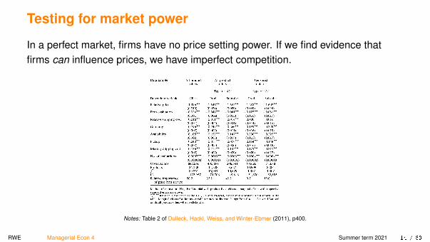
Testing for market power

In a perfect market, firms have no price setting power. If we find evidence thatfirms can influence prices, we have imperfect competition.

Notes: Table 2 of Dulleck, Hackl, Weiss, and Winter-Ebmer (2011), p400.


https://onlinelibrary.wiley.com/doi/epdf/10.1111/j.1468-0475.2011.00535.x

https://onlinelibrary.wiley.com/doi/epdf/10.1111/j.1468-0475.2011.00535.x

More on the results

� The authors find considerable price variation, Coefficient of Variation ≈ 0.1.1

� Firms differ (e.g., evaluation) which suggests that there is a trade-offbetween a cheaper price and firm characteristics.

� For some products, there are few suppliers: Ten more firms reduce markup by2.6 percentage points Hackl, Kummer, Winter-Ebmer, and Zulehner (2014).

1CoV = σ/|µ|, i.e., Standard deviation / | Mean |.RWE Managerial Econ 4 Summer term 2021 15 / 63

https://www.sciencedirect.com/science/article/pii/S0014292114000506

Monopoly

� Monopoly: the firm’s demand curve is the market demand curve.

� Monopolistically competitive firms: have (local) market power based onproduct differentiation, but barriers to entry are modest or absent.


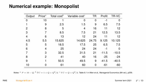
Numerical example: Monopolist

Output Pricea Total costb Variable costc TR Profit TR-VC0 10 1 0 0 -1 01 9 2.5 1.5 9 6.5 7.52 8 5 4 16 11 123 7 8.5 7.5 21 12.5 13.54 6 13 12 24 11 124.5 5.5 15.625 14.625 24.75 9.125 10.1255 5 18.5 17.5 25 6.5 7.56 4 25 24 24 -1 07 3 32.5 31.5 21 -11.5 -10.58 2 41 40 16 -25 -249 1 50.5 49.5 9 -41.5 -40.510 0 61 60 0 -61 -60

Notes: a P = 10 − Q. b TC = 1 + Q + Q2/2. c V C = Q + Q2/2. Table 8.1 in Allen et al., Managerial Economics (8th ed.), p259.


How much should the monopolist produce?

Demand: P = 10−QTR: TR = PQ = 10Q−Q2

TC: TC = 1 +Q+Q2/2

This implies: FC = 1

This implies: V C = Q+Q2/2

This implies: MC = ∂TC/∂Q = 1 +Q

maxπ = TR− TC = 10Q−Q2 − [1 +Q+Q2/2]

∂π/∂Q = 10− 2Q− [1 +Q] ⇒ Q = 3, P = 7.


Output and prices of a monopolist

A monopolist’s output decision determines the market price. (In contrast to amarket with perfect competition, where the output of one firm does not influencethe market price.)

� The MR(Q) is the difference between TR at one level of output and the TR ofproducing one more unit:

MR(Q) =∂TR

∂Q=∂P (Q)Q

∂Q=∂P

∂QQ+ P (Q)

= P

[1 +

∂P

∂Q

Q

P

]= P [1 + (1/η)] = P [1− (1/|η|)] = P − P/|η|.

(If demand is downward-sloping, η < 0.)


MR < P in a monopoly

MR = P [1 + (1/η)] < P :

� A profit-maximizing monopolist will not produce where demand is inelastic;that is, where |η| < 1, because MR < 0.

� MC = MR = P [1− (1/|η|)]; so the profit-maximizing price is

MC = P

[1−

(1

|η|

)]P =

MC[1−

(1|η|

)] .


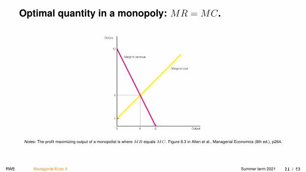
Optimal quantity in a monopoly: MR = MC.

Notes: The profit maximizing output of a monopolist is where MR equals MC. Figure 8.3 in Allen et al., Managerial Economics (8th ed.), p264.


A monopolist’s output and prices

Notes: 1. MR equals MC leads to QM ; 2. PM = P (QM ). Figure 8.4 in Allen et al., Managerial Economics (8th ed.), p265.


Monopoly lowers welfare

� Producer surplus: difference b/n marginal cost and price

� Consumer surplus: difference b/n willingness to pay and price

� Total welfare: producer surplus + consumer surplus

� A monopolist explicitly considers demand

� Why does no other firm enter the market?


Monopoly and market power

A monopolist has market power and raises prices above marginal cost. Theimpact of market power on social welfare:

� Allocative inefficiency: effect on welfare if market power is exerted (lessoutput, higher price)

� Productive inefficiency: effect on welfare if market power is exerted by atechnologically inefficient firm (less attention to marginal costs from lack ofcompetition)

� Dynamic inefficiency: lack of investment due to lower incentive to generatenew technologies (innovation)


Allocative inefficiency

Any price above marginal cost induces a net loss in social welfare.

Notes: In a competitive market, the total surplus from free trade is the area PcSO. In a monopoly market, the total surplus is the area PcTRPm .The welfare loss is the shaded area RST .


The determinants of welfare loss

� The more market power, the higher the price, hence the greater the welfareloss⇒ inverse relationship between market power and social welfare.

� The more elastic the demand curve with respect to price, the lower is thewelfare loss.

� The larger the market under consideration, the greater the welfare loss.


Rent-seeking activities

� The potential profits of a monopoly can lead firms to waste resources inunproductive lobbying activities to increase market power. The more firmstry this, the more is wasted.

� In the extreme, all the profits created under monopoly may be sacrificed onsuch activities, “full rent dissipation” (Posner, 1975).

� Conditions for full rent dissipation:� competition among the firms involved in rent-seeking� the rent-seeking activities do not have any social value


Productive inefficiency

A monopolist may produce at a higher marginal cost than a firm under perfectcompetition:

� Managers may not have the right incentives to adopt the most efficienttechnology, “managerial slack”

� Lack of competition does not force the firm to lower marginal costs


Dynamic inefficiency

A monopolist has lower incentives to innovate. Example:

� A new technology at fixed cost F allows the firm to produce at a lowermarginal cost cnew < cold

� Monopolist adopts the new technology if: Πnew −Πold > F

� A firm under perfect competition adopts the new technology if: Πnew > F


Other aspects of monopolies

� “Natural monopoly”: if there is a minimum efficient scale, i.e., the minimum ofaverage cost is only at very high output levels, there is only place for one firmin the market!

� Measure of monopoly power is the markup, µ, of price over cost:

markup = P−MCMC


Sources of monopoly power

� “Natural monopoly”: public utilities, railway tracks, economies of scale

� Capital requirements on production or big sunk costs on entry (e.g., powerplant)

� Law: Patents (17 years) or trade secrets (Coke)

� Exclusive or unique assets (minerals, talent)

� Exclusive location (popcorn shop in cinema—but in general you pay rent forthese advantages)

� Regulation (TV, taxi, radio frequency bands)

� Collusion by competitors


Strategic entry barriers

� Excessive patenting and copyright

� Limit pricing (set price below monopoly price)

� Extensive advertising to create brand name to raise cost of entry

� Create intentionally excess capacity as a warning for a price war

� “Predatory pricing”: drive competitors from the market with prices belowmarginal costs


Double marginalization

Consider two monopolies, an upstream company (whole sale company) and adownstream company (retailer).

Notes: The downstream company’s marginal revenue is the relevant demand for the upstream company; i.e. blue and green lines are the same! Achain of two monopolies results in even further welfare loss. This is easily seen, because the final MR curve is further to the left and prices increase.


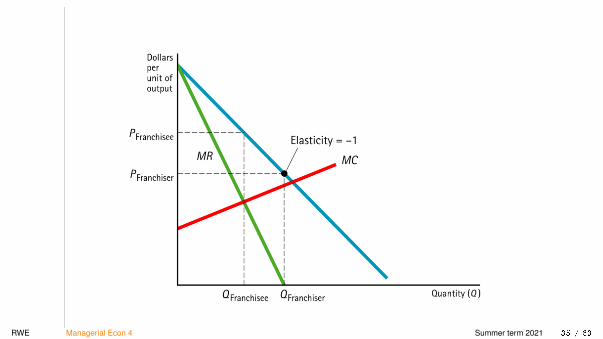
Franchising

Consider two monopolies, a franchisor (upstream company, whole sale company)and a franchisee (downstream company, retailer).

� The franchisor maximizes profits by (i) setting all intermediate goods atmarginal costs and (ii) extracting the monopoly rents of the franchisee bysetting a high franchise fee

� The franchisor grants the franchisee a local monopoly

� The franchise fee drives the franchisee to set P = MC

� The franchisee benefits from overall branding and advertising


Mark-up pricing

Managers almost always say that “prices are related to costs”, but rarely that theydepend on demand ...

1. The firm estimates the cost per unit of output of the product, usually averagecost

2. The firm adds a markup, µ, to the estimated average cost

P = (1 + µ)C.


Does mark-up pricing maximize profit?

Markup-pricing will maximize profit if:

� MC = MR⇒ P = MC/(1 + 1/η)

� Optimal Price: it is essential to know the elasticity of demand

� Marginal costs: these are typical known (however, firms rely often on averagecosts )


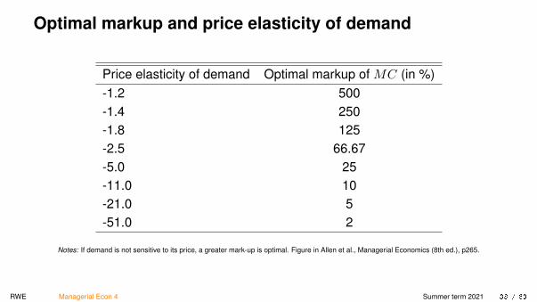
Optimal markup and price elasticity of demand

Price elasticity of demand Optimal markup of MC (in %)-1.2 500-1.4 250-1.8 125-2.5 66.67-5.0 25-11.0 10-21.0 5-51.0 2

Notes: If demand is not sensitive to its price, a greater mark-up is optimal. Figure in Allen et al., Managerial Economics (8th ed.), p265.


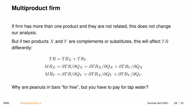
Multiproduct firm

If firm has more than one product and they are not related, this does not changeour analysis.

But if two products X and Y are complements or substitutes, this will affect TRdifferently:

TR = TRX + TRY

MRX = ∂TR/∂QX = ∂TRX/∂QX + ∂TRY /∂QX

MRY = ∂TR/∂QY = ∂TRX/∂QY + ∂TRY /∂QY

Why are peanuts in bars “for free”, but you have to pay for tap water?


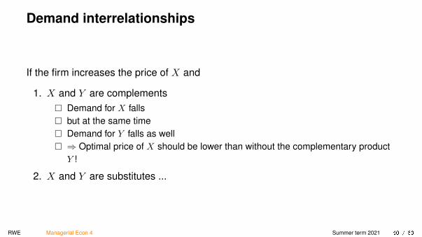
Demand interrelationships

If the firm increases the price of X and

1. X and Y are complements� Demand for X falls� but at the same time� Demand for Y falls as well� ⇒ Optimal price of X should be lower than without the complementary product

Y !

2. X and Y are substitutes ...


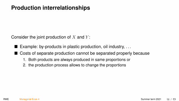
Production interrelationships

Consider the joint production of X and Y :

� Example: by-products in plastic production, oil industry, . . .� Costs of separate production cannot be separated properly because

1. Both products are always produced in same proportions or2. the production process allows to change the proportions


Joint production with fixed proportions

Notes: The intersection between the Total Marginal Revenue Curve (TMR), obtained from the vertical sum of the separate marginal revenue curves,and the marginal cost curve determines the optimal quantities (and prices). Figure 8.5 in Allen et al., Managerial Economics (8th ed.), p276.


Joint production with fixed proportions

The production of one good automatically produces the other

� Total marginal revenue, TMR: The summation of the two marginal revenuesfor individual products

� Pricing rule: TMR = MC.

� The marginal revenue (from both products) from producing one more unitshould be equal the marginal costs.


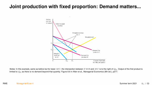
Joint production with fixed proportion: Demand matters...

Notes: In this example, same as before but for lower MC, the intersection between TMR and MC is to the right of Q0. Output of the first product islimited to Q0 as there is no demand beyond that quantity. Figure 8.6 in Allen et al., Managerial Economics (8th ed.), p277.


Joint production with variable proportions

Since production of X and Y may vary, we need to examine

� Iso-revenues: all combinations of output levels of X and Y that have the samerevenue

� Iso-costs: all combinations of output levels X and Y with same costs

� Tangency condition: profit is maximized, which occurs at a point of tangency


Joint production with variable proportions

Notes: The optimal output is determined by isorevenue lines and isocost curves. Isorevenue lines are the locations of all combinations of outputs whichyield the same revenues. Isocost curves are locations of all combinations of outputs that have the same costs. The tangent point of an isorevenue lineand an isocost curve that yields the highest profit determines the optimal output. Figure 8.7 in Allen et al., Managerial Economics (8th ed.), p280.


A single buyer

MonopsonyMarkets where there is only one buyer

� Early research by Joan Robinson

� Buyers on a competitive market face a horizontal supply curve; they are pricetakers.

� A monopsony faces an upward-sloping supply curve, they are price makers.


https://www.econlib.org/library/Enc/bios/Robinson.html

Discriminating monopsony

� The monopsonist can distinguish between sellers’ reserve prices or workers’reservation wages and pays each differently (optimally at their reservationprice or reservation wage).

� The supply curve is upward-sloping and co-incides with the marginal costcurve.

� The quantity bought (the number of workers hired) is the same as in acompetitive market.

� There is not one single price, but each supplier is paid a different price.


Non-discriminating monopsony

� The monopsonist cannot distinguish between sellers (workers).

� If the monopsonist wishes to buy more raw materials (or to hire moreworkers), it has to pay the same greater price (wage) for all.

� The supply curve is upward-sloping; the marginal expenditures are above thesupply curve.

� The monopsonist will purchase a quantity (hire the number of workers) wheremarginal expenditures are equal to the demand curve (which co-incides withthe marginal revenue product).

� The monopsonist will pay a price below marginal cost.

� The quantity bought is less than in a competitive market; the price is lowerthan in a competitive market.


The optimal quantity that a monopsonist buys

Notes: A (non-discriminating) monopsonist faces an upward-sloping supply curve. The optimal quantity. Q∗, is given by the intersection of themarginal expenditure curve with the demand curve. The optimal price, P∗, the monopsonist pays is the price resulting from its purchase of Q∗ units.The area D, a triangle in this diagram, indicates the loss in welfare due to unrealized trades.


Monopolistic competition (mcm)

In a competitive market, firms aim to create at least a “local monopoly”:

� Spatial differences: This is the true “local” aspect, e.g., a restaurant car on atrain. Very difficult to switch to a different restaurant ...

� Product differences: Firms aim to convince consumers that their products aredifferent to the competitors’ products, e.g., using brands

� In a monopolistically competitive market (mcm), managers have some pricingpower, but because products are similar, the price differences a relativelysmall.

� In other words, in a mcm, the demand curve for an individual firm is not flat.

� Other conditions are as in a competitive situation, i.e., many firms and freeentry into the market.


Prices in a mcm

What happens if firm changes price alone (dd) or if all firms change their prices(DD)?

� Consider a very small firm which changes the price, its demand curve is veryflat

� Marketing is important: firms want to make their product “unique”

� If a product is “special”, the demand becomes more inelastic (steeper)

� If all firms change the price at the same time, no consumer can switch tocompetitor


MCM: One firm vs. all firms

Notes: The effect of price changes in a market with monopolistic competition depends on how many firms are changing their prices. If one firmreduces the price from P0 to P1 , the supplied quantity changes from Q0 to Q′1. If many or all firms change their prices, the overall demand curve,DD, pivots and the quantity supplied changes to Q1.


Short-run and long-run outcomes in a mcm

Firms aim to behave like monopolists and set the price where MR = MC.

� This results in profits — remember, economic profits 6= accounting profits!

� The potential to make profits attracts other firms to enter the market

� Each firm competes for a share of total demand and entry lowers the demandfor the individual firm

� In the long run, profits disappear and the demand curve becomes tangentialto the long-run average cost curve


Short-run equilibrium in a mcm

Notes: A firm in a mcm will produce Q0 units of output as this is the quantity where MR = MC. The price is given by the demand curve,P = P (Q), and is indicated by P0 . The firm will obtain profits of P0 − C0 per unit of output. Figure 8.9 in Allen et al., Managerial Economics (8thed.), p284.


Long-run equilibrium in a mcm

Notes: In the long term, firms will enter the mcm and lower profits.Firms will produce where MR = MC, i.e., Q1. The price is givenby the demand curve, P = P (Q), and is indicated by P1. Notethat MC are at a minimum at a greater quantity, Q2. Figure 8.9 inAllen et al., Managerial Economics (8th ed.), p284.

� Profits attract entrants

� Market entry lowers demand theindividual firm

� Zero profit condition met(TR = TC)

� Profit-maximization conditionmet (MC = MR)

� Production is not cost-efficientas long-run average costs not atminimum

� This is the “cost” of productvariety


MCM

� Common type of market

� No interaction between firms

� Firm could reduce average cost by producing more� Firms aim to bind their costumers to the firm:

� Marketing and advertising is important (loyalty schemes, better taste, ...)� Product differentiation to achieve “local monopoly”


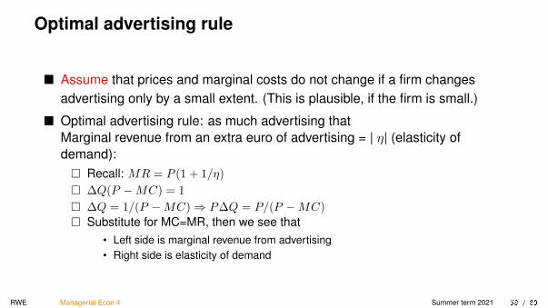
Optimal advertising rule

� Assume that prices and marginal costs do not change if a firm changesadvertising only by a small extent. (This is plausible, if the firm is small.)

� Optimal advertising rule: as much advertising thatMarginal revenue from an extra euro of advertising = | η| (elasticity ofdemand):� Recall: MR = P (1 + 1/η)

� ∆Q(P −MC) = 1

� ∆Q = 1/(P −MC)⇒ P∆Q = P/(P −MC)

� Substitute for MC=MR, then we see that• Left side is marginal revenue from advertising• Right side is elasticity of demand


Numerical example: Optimal advertising rule

Assume:

� η = -1.6

� Managers believe that an extra e100,000 of advertising will increase sales bye200,000, i.e., E[MR] = 2. (E[·] indicates the expectations.)

� A manager can increase profits by advertising more; MR > |η|.� To maximize profits, the manager should increase advertising to the point

where the return to an extra euro of advertising falls to 1.6.


Optimal advertising expenditure: advertising meant toincrease brand consciousness of clients

� With little advertising, elasticity will be high, because product will beconsidered as easily substitutable to others,

� Increase advertising and elasticity will fall


Strategic advertising

A firm may choose between two strategies

1. Low-price strategy, “promotions” to increase the price elasticity:� Advertise price cuts to increase the price consciousness of customers

2. High-price strategy, to increase brand consciousness:� Price elasticity of demand should decrease (demand curve should get steeper)


Price elasticity and advertising

Own-price elasticity of demandBrand Advertised price change Unadvertised price changeChock Full o’nuts -8.9 -6.5Maxwell House -6.0 ∗

Folgers -15.1 -10.6Hill Brothers -6.3 -4.2

Notes: ∗ Not statistically significantly different from zero. Katz and Shapiro, 1986, “Consumer Shopping Behavior in the Retail Coffee Market”, Table14, p443.


Price promotions

� Promotions increase the price elasticities of consumers

� Promotions have less effect on brand loyality

� The effects of promotions decay over time

� Price elasticity of disloyal customers is four times greater than of loyalcustomers

� The effects of advertising on brand loyalty erode over time and prices becomemore important to consumers.


managerial economics lecture 4: market types

Documents