managerial and organizational efficiency applied ... · managerial and organizational efficiency...
TRANSCRIPT
Managerial and Organizational Efficiency –
Applied Econometrics in Professional Team
Sports
Der Fakultät für Wirtschaftswissenschaften der
Universität Paderborn
zur Erlangung des akademischen Grades
Doktor der Wirtschaftswissenschaften
- Doctor rerum politicarum -
vorgelegte Dissertation
von
Arne Büschemann, M.A.
geboren am 17.02.1982 in Lage, Lippe
Paderborn, 2015
Fakultät für Wirtschaftswissenschaften Lehrstuhl für Organisations-, Medien- und Sportökonomie

Vorwort
An dieser Stelle möchte ich die Gelegenheit nutzen, mich bei all denen Personen zu
bedanken, die mich während meiner Promotionsphase fachlich, aber auch persönlich
begleitet und unterstützt haben.
Allen voran möchte ich meinem Doktorvater Prof. Dr. Bernd Frick für die optimale
Betreuung und sein Vertrauen während meiner Zeit als wissenschaftlicher Mitarbeiter
am Lehrstuhl, aber auch insbesondere für die Zeit danach als externer Doktorand
danken.
Des Weiteren möchte ich den Gutachtern Prof. Dr. Joachim Prinz, Prof. Dr. Martin
Schneider und Prof. Dr. Burkhard Hehenkamp für Ihre Bereitschaft als Zweitgutachter
bzw. Promotionskommissionsmitglieder mitzuwirken und für die fachlich äußerst
bereichernde Diskussion im Rahmen der Disputation danken. Mein besonderer Dank
gilt Prof. Dr. Joachim Prinz, der mir insbesondere zu Beginn meiner Promotionsphase
eine große Unterstützung gewesen ist.
Mein Dank gilt außerdem meinem Freund und Koautor bei diversen Fachartikeln, Prof.
Dr. Christian Deutscher, für die herausragende Zusammenarbeit auf und abseits des
Courts. Meinen Kolleginnen und Kollegen am Lehrstuhl, Dr. Filz Şen, Dr. Linda Kurze
und Dr. Marcel Battré danke ich für eine Zusammenarbeit, die einmalig gewesen ist.
Den studentischen Hilfskräften danke ich für ihre tatkräftige Unterstützung bei der
Fertigstellung von Datensätzen. Meinem Arbeitgeber „Vodafone“, für die Möglichkeit
mein Promotionsvorhaben zeitlich flexibel fortzuführen.
Abschließend möchte ich mich bei meinen Eltern, meinen Freunden und meiner
Freundin Anastasija für die grenzenlose Unterstützung, die unermüdliche Geduld und
die nötige Ablenkung bedanken.
Arne Büschemann Düsseldorf, im April 2015

I
Table of Contents
Table of Contents ............................................................................................................. I
List of Figures ............................................................................................................... III
List of Tables ................................................................................................................. IV
List of Abbreviations ...................................................................................................... V
1 Introduction ........................................................................................................... 1
2 The Trade-Off between High Scoring Games and Competitive
Balance in Basketball .......................................................................................... 10
2.1 Introduction .......................................................................................................... 10
2.2 Competitive Balance and its Drivers ................................................................... 11
2.3 Data and Results .................................................................................................. 13
2.3.1 Short, Mid- & Long-Term Effects ............................................................. 14
2.3.2 Game-Level Measures ............................................................................... 14
2.3.3 Season-Level Measures ............................................................................. 17
2.4 Discussion and Conclusion .................................................................................. 18
2.4.1 Limitations ................................................................................................. 18
2.4.2 Implications ............................................................................................... 19
3 Did the 2005 Collective Bargaining Agreement Really Improve
Team Efficiency in the NHL? ............................................................................ 21
3.1 Introduction .......................................................................................................... 21
3.2 Data Description .................................................................................................. 24
3.3 Empirical Analyses of Efficiencies ..................................................................... 27
3.4 Conclusions .......................................................................................................... 33
4 Sport or Business Approach? A Cross-Continent Analysis of U.S.
Major League Franchises and English Premier League Clubs ...................... 34
4.1 Introduction .......................................................................................................... 34
4.2 Literature Review ................................................................................................ 36
4.3 Data set and Descriptive Statistics ....................................................................... 40
4.4 Empirical Regression Model ............................................................................... 45
4.5 DEA Efficiency Model ........................................................................................ 45

II
4.6 Econometric Findings .......................................................................................... 47
4.6.1 Results of the Fixed-Effect Regression ..................................................... 47
4.6.2 DEA Efficiency Results............................................................................. 50
4.7 Summary and Concluding Remarks .................................................................... 53
5 Does Performance Consistency Pay-Off Financially for Players?
Evidence from the Bundesliga ........................................................................... 55
5.1 Introduction .......................................................................................................... 55
5.2 Literature Review ................................................................................................ 56
5.3 Data Set and Descriptive Statistics ...................................................................... 62
5.4 Econometric Findings .......................................................................................... 68
5.5 Summary and Concluding Remarks .................................................................... 74
6 Environmental Regulations and the Relocation of Production: A
Panel Analysis of German Industry Investment Behaviour ........................... 77
6.1 Introduction .......................................................................................................... 77
6.2 Literature Review ................................................................................................ 78
6.3 Empirical Model .................................................................................................. 83
6.4 Panel Data Description ........................................................................................ 85
6.5 Empirical Results ................................................................................................. 91
6.5.1 Descriptive Statistics ................................................................................. 91
6.5.2 Empirical Results on an aggregated level.................................................. 95
6.5.3 Empirical Results on the industry level ..................................................... 97
6.6 Discussion .......................................................................................................... 103
7 Conclusion and Outlook ................................................................................... 106
8 Bibliography ........................................................................................................ VI
III
List of Figures
Figure 2-1: Observation periods surrounding the rule change in 2000 .......................... 14
Figure 3-1: Team efficiencies prior to and after the Lockout for the dependent
variable log(Value) .......................................................................................................... 32
Figure 3-2: Team efficiencies prior to and after the Lockout for the dependent
variable log(Revenue)...................................................................................................... 32
Figure 5-1: Average expert ratings by position .............................................................. 67
Figure 5-2: Variation coefficient of performance by players´ position .......................... 68
Figure 5-3: Kernel Density Estimates of player salaries ................................................ 72
Figure 5-4: Reward scheme Bundesliga ......................................................................... 76
Figure 6-1: The share of pollution abatement investment in total investment ............... 86
Figure 6-2: Annual change of outbound FDI in percent ................................................ 92
Figure 6-3: Total outbound FDI by industry in billion € ................................................ 93
Figure 6-4: German FDI growth rates of countries with low/strict regulations ............. 94

IV
List of Tables
Table 2-1: Poisson regression: Marginal effects on score differences ........................... 15
Table 2-2: Poisson regression: Marginal effects on total points scored ......................... 16
Table 2-3: Season-level measures of the effects of shot clock rule changes .................. 18
Table 3-1: Descriptive Statistics of indicators influencing team values ........................ 27
Table 3-2: Stochastic Frontier Estimate for the dependent variable log(Value) ............ 29
Table 3-3: Stochastic Frontier Estimate for the dependent variable log(Revenue) ........ 30
Table 4-1: Literature on determinants of franchise values ............................................. 37
Table 4-2: Literature on data envelopment analysis in sport.......................................... 39
Table 4-3: Descriptive statistics ..................................................................................... 44
Table 4-4: Estimates of the fixed-effects regression ...................................................... 49
Table 4-5: Global technical efficiency scores for sporting efficiency............................ 50
Table 4-6: Global technical efficiency scores for financial efficiency ........................... 52
Table 4-7: Global technical efficiency margin scores of sporting and financial
efficiency ......................................................................................................................... 52
Table 5-1: Literature on salary determination for professional soccer ........................... 60
Table 5-2: Overview of variables ................................................................................... 65
Table 5-3: Summary of descriptive statistics ................................................................. 66
Table 5-4: Estimation results for OLS and fixed-effects regressions ............................. 70
Table 5-5: Impact of consistent performance on salary (Quantile Regressions) ............ 73
Table 6-1: Overview and definition of variables ............................................................ 90
Table 6-2: Descriptive Statistics Total German outbound FDI ...................................... 91
Table 6-3: Determinants of Total German outbound FDI .............................................. 96
Table 6-4: Determinants of German outbound FDI in the manufacturing industry ....... 99

V
List of Abbreviations
ACB Asociación de Clubs de Baloncesto
CBA Collective Bargaining Agreement
DEA Data Envelopment Analysis
EPL English Premier League
FCI Fan Cost Index
FDI Foreign Direct Investment
FE Fixed-Effects
FFP Financial Fair Play
FIFA Fédération Internationale de Football Association
GCR Global Competitiveness Report
GDP Gross Domestic Product
GDPPC Gross Domestic Product Per Capita
IMF International Monetary Fund
IPPS Industrial Pollution Projection System
MLB Major League Baseball
MNE Multinational Enterprise
NBA National Basketball Association
NFL National Football League
NHL National Hockey League
NHLPA National Hockey League Players´Association
OLS Ordinary Least Squares
RE Random-Effects
SFA Stochastic Frontier Analysis
SMSA Standard Metropolitan Statistical Area
UEFA Union Européenne de Football Association
Chapter 1: Introduction
1
1 Introduction
Since the article pioneering the concept of sports economy was published by
Simon Rottenberg in 1956, academic studies of professional team sports have steadily
expanded and gained attention, especially in the past two decades, when substantial
increases in both the demand and supply of professional sport teams have combined
with greater professionalism among stakeholders. Rottenberg’s (1956) uncertainty of
outcome hypothesis predicted that, other things being equal, closer competition between
teams and across a professional sport league would increase spectators’ interest in the
sport and attendance rates. Attendance strongly determines the revenues of professional
sport teams and companies associated with the industry, and the increased demand and
supply can be best illustrated with data from a single game, the 2014 World Cup Final
in Brazil. The combined market value of the teams in the final, Argentina and Germany,
amounted to €951 million.1 On average 53,592 spectators attended 64 World Cup
games, for nearly 3.5 million attendees throughout the tournament. Even more
impressive are the national and global television ratings: In Germany, they reached an
all-time high, with a market share of 86.3% and 34.65 million spectators. Across the
globe, an audience of more than 1 billion tuned in to this single game.2
In addition to being extremely popular, the professional sports industry differs
from any other. For example, a monopoly is neither a profitable nor a desirable state for
market participants, because the final good is a joint production of the contestants in
each league, single game, or contest (Neale, 1964). The stronger the contenders, the
greater the profits are, in line with the uncertainty of outcome hypothesis. To maintain
1 AGF/GfK Fernsehpanel 13.07.2014.
2 Data obtained from www.transfermarkt.de, though the data on the final global television audience
remains unofficial; http://www.bbc.com/sport/0/football/28278945 12.07.2014.

Chapter 1: Introduction
2
outcome uncertainty, sports economists cite the need for competitive balance; as many
studies show, competitive balance correlates with attendance, such that attendance
increases when competing teams are more evenly balanced (Forrest & Simmons, 2002;
Krautmann & Hadley, 2006; Meehan, Nelson, & Richardson, 2007; Lee & Fort, 2008;
Lee, 2009). Measures to maintain or even increase competitive balance include salary
caps, revenue sharing, luxury taxes, reverse-order drafts, and exemptions from antitrust
law, all which are predominantly applied in U.S. professional leagues (Fort & Quirk,
1995; Szymanski, 2003).
In European sports leagues, such policies were largely absent before 2009, when
the administrative body of the European football association (UEFA) implemented its
Financial Fair Play (FFP) regulations. These regulations limit teams to spending no
more than they earn, even those teams owned by wealthy owners who are willing to
invest private money to strengthen their squads and whose habits had begun prompting
most teams to overspend to remain competitive (Sass, 2012). Teams that fail to comply
with these regulations face the threats of severe financial penalties, transfer bans, and
exclusion from international competitions.
Increasing regulations in turn force professional sport teams to strive even harder
for superior organizational performance. The organizational goals and outcomes are
much clearer for professional team sports than for companies in most other industries.
Their key objectives, given their available resources, are sport success and business
performance (Guzmán, 2006). Usually, better sport performance translates into greater
revenues and profits for team owners (Frick & Simmons, 2008), but superior business
performance depends not just on the organization’s resource endowment but also on the
efficiency with which the team uses this endowment (Gerrard, 2005). This notion

Chapter 1: Introduction
3
resonates with the resource-based view (RBV), a popular theoretical model of how
firms use their resources and capabilities strategically to achieve objectives in an
efficient manner (Rumelt, 1984; Wernerfelt, 1984; Barney, 1991). Specifically, the
RBV provides a framework for identifying, defining, and attaining a sustainable
competitive advantage through the effective, efficient deployment of each firm’s rare,
valuable resources, which are neither perfectly imitable nor substitutable without great
effort (Barney, 1991; Peteraf, 1993). That is, the following four attributes of a resource
must exist for a resource to enable above-normal economic rents: It must be valuable,
rare, in-imitable and non-substitutable, as summarized by the VRIN model (Barney,
1991):
1. It must be valuable, in that it exploits opportunities or neutralizes threats in the
firm’s environment.
2. It must be rare among the firm’s current and potential competition.
3. It must be imperfectly imitable.
4. It must be non-substitutable, so there cannot be strategically equivalent
substitutes that are valuable but neither rare nor imperfectly imitable.
A resource is any asset, capability, organizational process, attribute, information,
or knowledge controlled by a firm that enables it to conceive of and implement
strategies to improve its efficiency and effectiveness (Barney, 1991).3 Thus,
outperforming competitors requires more than the availability of resources; it also
requires the firm to convert its own resources into effective processes. Consequently,
3 A more general definition by Wernerfelt (1984) refers to a resource as anything that could be thought of
as a strength of a given firm.
Chapter 1: Introduction
4
the ability to exploit resources better than competitors is a key competency (Reed &
DeFillippi, 1990).
As an extension of this view, the VRIO framework adds the consideration of
whether the firm is appropriately organized to exploit the resource (Barney, 1995). The
rationale for adding this factor is the notion that to realize the potential of a valuable,
rare, and costly to imitate resource, the firm must be organized in such a way that it can
capture that value, as determined by its formal reporting structure, management control
systems, or compensation policies, for example (Barney, 1995).
For professional sports teams, the human capital of their players represents both a
primary resource and a key expense. However, players cannot be considered strategic
resources, because an effective and regulated labor market exists for them. Rather, the
abilities to identify future top players and recruit them, using superior scouting
capabilities, represent competencies and resources that might lead to a competitive
advantage. In addition, the ability to exploit market inefficiencies and sign players at
prices below their marginal revenue contributions constitutes another strategic resource.
Fritz (2006) cites several other resources and competencies that possess the potential to
invoke competitive advantages, such as drawing potential, or the market potential that a
given infrastructure produces. This market potential depends on various factors,
including population, income per capita, and the history and reputation of the team.
Finally, superior marketing capabilities, which might increase sponsorship revenues,
and the competency to create effective player and coaching squads are resources with
strong influences on sport and financial success.
Chapter 1: Introduction
5
This dissertation seeks to answer several research questions related to this field
empirically. Accordingly, I have gathered data sets from various professional sports,
including data about the team-level financial and sport performance of four North
American major sport leagues: the National Basketball Association (NBA), National
Hockey League (NHL), National Football League (NFL), and Major League Baseball
(MLB), as well as from English Premier League (EPL) clubs. I use detailed individual
player performance and salary data related to players in the German Bundesliga. My
analyses also rely on game- and season-level data from the Spanish basketball top
division Asociación de Clubs de Baloncesto (ACB). The financial performance data of
professional sport teams are inherently scarce though. For the U.S. team sports, I
gathered industry information about team values and revenues from Forbes Magazine.
For European soccer teams, Forbes only reports team values for the 25 most valuable
clubs, not entire national leagues. To analyze the financial performance of EPL clubs, I
turned to data provided by Deloitte & Touche GmbH, which calculates and publishes
revenues in its Annual Review of Football Finance Report.
With these data, I start with an initial assessment of the uncertainty of outcome
hypothesis in Chapter 2, by empirically detailing the trade-off between scoring and
competitive balance in professional basketball. When it reduced the time of possession
from 30 seconds to 24 seconds in 2000, the Spanish basketball federation sought to
increase the speed and attractiveness of the game. Two main consequences should result
from this rule change. First, the number of points scored per game should increase, due
to the greater number of possessions and shot attempts. Second, competitive balance
should decrease, because in any game, relative team inequality implies that an increase
in possessions will enhance the chances of the better team to win. Using both game- and
Chapter 1: Introduction
6
season-level data from the Spanish professional league, Chapter 2 confirms that a
resulting increase in scoring was accompanied by decreased competitive balance. This
finding empirically reveals the trade-off between these two measures, both of which
presumably could drive consumer demand. The implications are straightforward: If a
sport’s governing body is tempted to increase the speed of the games, it faces a
significant drawback, in the form of fewer surprising outcomes and less competitive
balance, in conflict with recommendations derived from the uncertainty of outcome
hypothesis.4
Chapter 3 addresses the financial performance of NHL franchises, prior and after
a new collective bargaining agreement (CBA) in 2005, which provides an unique setting
in which to analyze the impact of a regulatory intervention on managerial efficiency.
The new CBA followed the cancelled 2004–05 season, when team owners and the
National Hockey League Players’ Association (NHLPA) could not reach agreement on
a key point. Team owners demanded cost certainty, noting that player salaries consumed
more than 65% of the generated revenues, whereas the NHLPA refused to install salary
restrictions. The 2005 CBA introduced both salary regulations and revenue sharing to
the NHL, in a bid to restore financial competitiveness. With these objectives, the key
question is whether the new CBA actually improved efficiency. Using team values as
the dependent variable, I show that an abrupt increase in technical efficiencies resulted
from the CBA; in particular, poorly performing teams benefited from the newly
introduced measures.5
4 A version of this chapter, “The Trade-Off between High Scoring Games and Competitive Balance in
Basketball,” has been submitted for publication consideration to Journal of Sport Economics
(Büschemann & Deutscher, 2014). 5 A version of this chapter, “Did the 2005 Collective Bargaining Agreement Really Improve Team
Efficiency in the NHL?” was published in International Journal of Sports Finance (Büschemann &
Deutscher, 2011).
Chapter 1: Introduction
7
With Chapter 4, I extend the efficiency analysis to all North American major
league franchises and clubs from the English Premier League, investigating the
differences in motives between North American and European sport teams, as well as
how sporting performance might differentially influence teams’ value and revenues.
Prior literature suggests that North American team owners tend to be profit-maximizing
business people, whereas European team owners are sportsmen and -women. Rather
than maximize profits, the sporting group is willing to sacrifice profits to win, such that
they ultimately become win maximizers who seek to win at any cost. Yet empirical
evidence of this difference remains scarce. Chapter 4 constitutes the first study to
analyze cross-continental empirical data and thereby close a research gap, as well as
suggest a novel approach for analyzing the determinants of financial performance and
the financial and athletic efficiency of professional sport teams. Using data related to
162 teams’ financial and sport performance over nine consecutive seasons (i.e., 1,237
team–season observations from 2001–02 to 2009–10), I show empirically that European
teams value athletic achievements differently than do U.S. major league franchises,
across several sports. The application of data envelopment efficiency analyses affirms
these findings.6
In Chapter 5, I turn to an analysis at the individual player level to identify
determinants of wage dispersions across professional athletes. Several individual
characteristics (e.g., age, experience, talent, position, team effects, country of origin,
and especially average performance) likely determine player salaries. This chapter
investigates how the consistency of professional soccer players’ performance might
6 A version of this chapter, “Sports or Business Approach? A Cross-Continent Analysis of U.S. Major
League Franchises and English Premier League Clubs” has been submitted for publication consideration
to European Sports Management Quarterly (Büschemann, 2014).

Chapter 1: Introduction
8
affect their salaries. The data set encompasses 845 different players who played in the
German Bundesliga between the 2005–06 and 2009–10 seasons, or 34,413 player–
match day observations. To measure performance consistency, I calculated a variation
coefficient over each season using player evaluations compiled by experts and
published in Kicker Sportmagazin, a highly respected soccer magazine. Strong
empirical evidence indicates that a salary premium rewards players who exhibit
performance volatility. Applying ordinary least squares, fixed effects, and quantile
regression analyses to disentangle the influence of performance for different parts of the
salary distribution, I show that this effect is robust.7
Finally, Chapter 6 offers a broader focus and integrates another field of research,
by analyzing the effects of environmental regulations on the foreign direct investment
(FDI) patterns of German multinational enterprises. Along the lines of inquiry
formulated by the so-called pollution haven hypothesis, a traditional economic view
suggests that countries with low environmental monitoring and regulations attract
multinational enterprises engaged in pollution-intensive production. Yet this hypothesis
still lacks empirical support. The applied panel data set contains information about
aggregated German outbound FDI and outbound FDI for selected industries from 2000
to 2006. To test for a statistically significant relationship between German FDI and
environmental regulations, I employed an environmental ranking published by the
World Economic Forum for each year of the sample period. The results reveal that
aggregated FDI is indeed redirected toward pollution havens, and this trend is especially
evident in polluting industries such as the chemical industry. The results for the
automotive industry show instead that FDI follows strict environmental regulations.
7 A version of this chapter, “Does Performance Consistency Pay Off Financially for Players? Evidence
from the Bundesliga,” appeared in Journal of Sport Economics (Deutscher & Büschemann, 2014).

Chapter 1: Introduction
9
These results support the Porter hypothesis and reveal that strong future market
potential may create a bias against a pollution haven effect.
Chapter 7 concludes this dissertation by summarizing the results and providing an
outlook for further research areas.

Chapter 2: The Trade-Off between High Scoring Games and Competitive Balance in
Basketball
10
2 The Trade-Off between High Scoring Games and Competitive
Balance in Basketball
2.1 Introduction
In sport contexts, institutional rule changes often seek to level the playing field for
teams or increase the attractiveness of the sport to consumers. In basketball for example,
the U.S. National Basketball Association (NBA) sought to reduce the domination of
physically superior players such as George Mikan or Wilt Chamberlain and increase
competitive balance. Recent rule changes in European basketball leagues have
prompted closer assimilation with the rules of the NBA, such as the 24-second shot
clock. European basketball leagues adopted this rule in 2000, which represented a
decrement from the previous time limit of 30 seconds. The goal was to increase the
speed of the game and accordingly increase the number of possessions, which should
have two main consequences: First, the number of points scored per game should
increase, with the greater number of possessions and shot attempts. Second, competitive
balance should decrease, because in any game, relative team inequality implies that the
increase in possessions will enhance the chances of the better team to win: More
repetitions reduce the impact of randomness on outcomes (Groot, 2009). The lessening
impact of randomness in turn should reduce competitive balance across the league.
With this study, we provide a novel empirical analysis of the trade-off between
the pace of the game and competitive balance, across 20 seasons of Spanish basketball.
We find that scoring improved significantly with the introduction of the shorter shot
clock, but competitive balance decreased significantly. The finding offers advice to the

Chapter 2: The Trade-Off between High Scoring Games and Competitive Balance in
Basketball
11
organizers of sports, especially for the open league system in Europe where regulations
aiming to increase competitive balance are rather hard to imply.
In the next section, we present an overview of studies that address competitive
balance in team sports. The data for the empirical analysis and the empirical results
appear in Section 3. We conclude with a discussion of these empirical results and an
outlook on further research in Section 4.
2.2 Competitive Balance and its Drivers
Research into competitive balance in professional team sports has a long history,
starting with Rottenberg’s (1956) uncertainty of outcome hypothesis. That is, in the
absence of regulation policies, teams located in larger markets sign the most talented
players, resulting in predictable match outcomes, which ultimately lead to lower
attendance. Neale (1964) similarly argues for the economic importance of team parity in
professional sports leagues, to maximize the profits earned by league participants. Most
previous analyses focus on North American team sports, particularly Major League
Baseball (MLB), and the effects of competitive balance on attendance. They offer
consistent support for the hypothesis that attendance is higher when competing teams
are more evenly balanced (Forrest & Simmons, 2002; Krautmann & Hadley, 2006;
Meehan, Nelson, & Richardson, 2007; Lee & Fort, 2008; Lee, 2009).
Sometimes unplanned changes affect competitive balance though. For example,
following the judgment of the European Court of Justice in 1995 in the Bosman
ruling—which pertained to whether players should be free to change teams when their
contracts have expired—within-season competitive balance increased, according to
Flores, Forrest, and Tena (2010). However, research into the effects of planned

Chapter 2: The Trade-Off between High Scoring Games and Competitive Balance in
Basketball
12
institutional changes, including rule changes, on competitive balance remains sparse.
Daly and Moore (1981) on the introduction of the MLB draft, and Croix and Kawaura
(1999) on the implementation in the Japanese Professional Baseball league find that
competitive balance improved after the introduction of a draft. Kent, Caudill, and
Mixon (2013) examine the effects of three rule changes on competitive balance that
occurred in 1958, 1970 and 1992 relating to player substitutions, to yellow card
penalties and to back-pass delaying tactics of seven European professional soccer
leagues, and find mixed evidence regarding match competitiveness, which they
measured by the score differential. According to Mastromarco and Runkel’s (2009)
empirical evidence, the Formula 1 organizational body frequently changes its rules to
improve competitive balance and maximize profits. They assert that the number of rule
changes depends on the competitive balance in the preceding season. Greater imparity
in season t – 1 increases the probability of rule changes at the start of season t.
Various measures might help maintain or increase competitive balance, such as
salary caps, revenue sharing, luxury taxes, reverse draft order picks, and exemptions
from antitrust law, most of which have been applied in major U.S. sport leagues (Fort &
Quirk, 1995; Szymanski, 2003). In European sports leagues, prominent policies include
financial fair play (FFP), as implemented by the UEFA, and a change in the point
awarding system by European football. Sass (2012) predicts the long-term effects of the
competitive balance resulting from FFP and finds a negative influence. The change in
the point system (from a 2-1-0 to a 3-1-0 scheme) also appears to have promoted greater
competitive imbalance (Haugen, 2008).

Chapter 2: The Trade-Off between High Scoring Games and Competitive Balance in
Basketball
13
These studies explicitly measure the impacts of rule changes on competitive
balance, without accounting separately for any impact of increased game speed on
competitive balance. Yet rule changes generally aim to make the sport more attractive
by increasing its pace, which simultaneously decreases competitive balance. With this
empirical study, we propose a novel perspective on the trade-off that regulators face,
between increasing the attractiveness of the game and maintaining competitive balance.
2.3 Data and Results
The data for this study comes from 20 seasons of the Spanish top division
Asociación de Clubs de Baloncesto (ACB). The Spanish national team has performed
well in international competition and also helped encourage successful league
competition. Over the 20 seasons we consider, Spanish teams advanced to the finals of
the Euroleague, the highest tier in professional basketball competition in Europe, 9
times. The data span all games played between the 1990-91 and the 2009-10 season, or
10 seasons before and 10 seasons after the introduction of the shorter shot clock in
2000–01. In most of these seasons, the league featured 18 teams, each of which played
all the others twice each season, providing 306 total observations. We gathered
information about the final score of the game, game day, and opponents. By aggregating
the regular season scores and comparing them against the final standings, we
determined our competitive balance measures. Furthermore, to assess the impact of the
shot clock change on scoring and competitive balance, we distinguished game-level and
season-level measures for various time intervals.
Chapter 2: The Trade-Off between High Scoring Games and Competitive Balance in
Basketball
14
2.3.1 Short, Mid- & Long-Term Effects
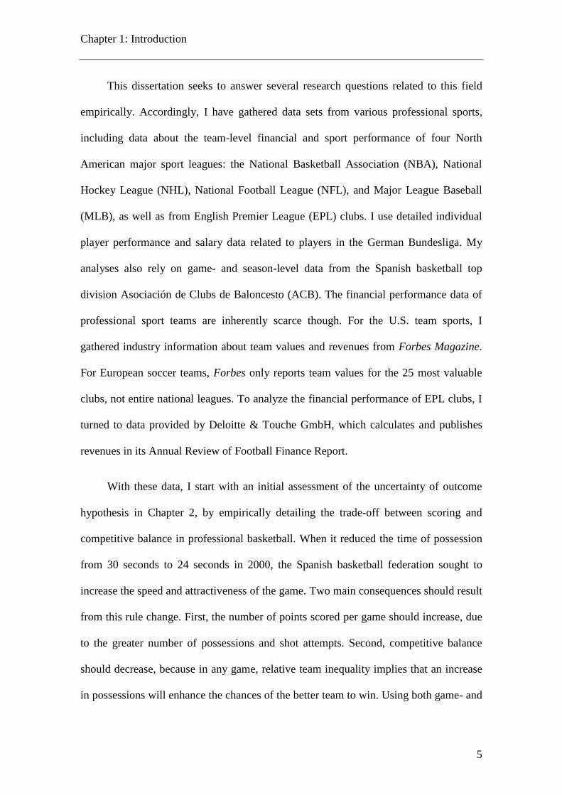
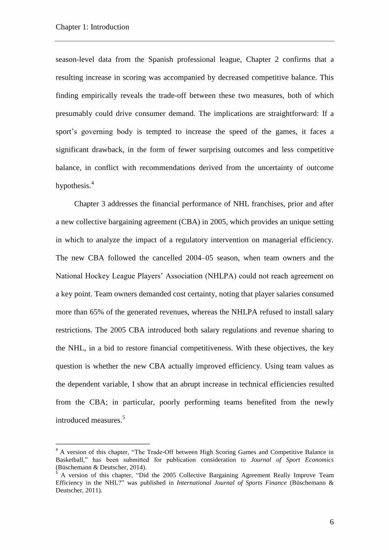
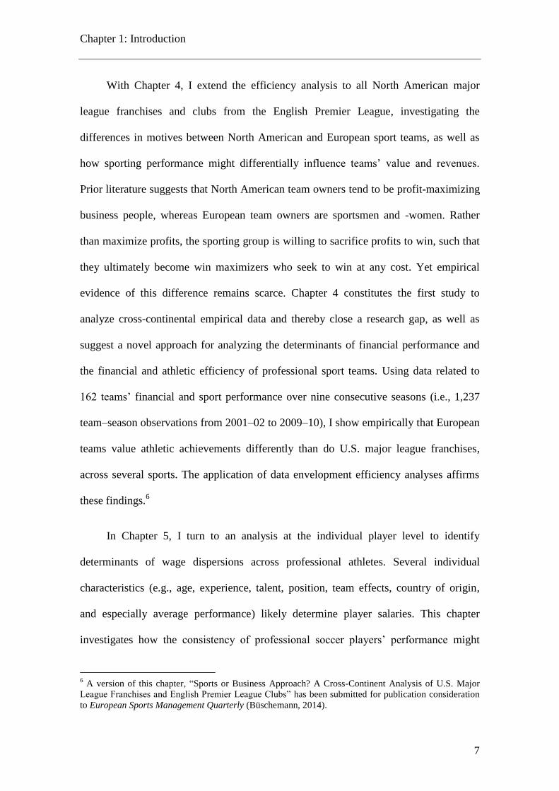
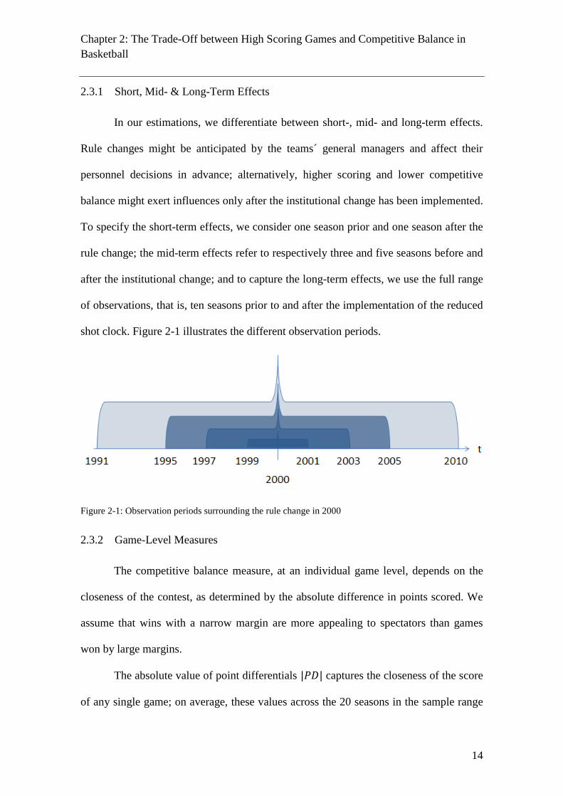
In our estimations, we differentiate between short-, mid- and long-term effects.
Rule changes might be anticipated by the teams´ general managers and affect their
personnel decisions in advance; alternatively, higher scoring and lower competitive
balance might exert influences only after the institutional change has been implemented.
To specify the short-term effects, we consider one season prior and one season after the
rule change; the mid-term effects refer to respectively three and five seasons before and
after the institutional change; and to capture the long-term effects, we use the full range
of observations, that is, ten seasons prior to and after the implementation of the reduced
shot clock. Figure 2-1 illustrates the different observation periods.
Figure 2-1: Observation periods surrounding the rule change in 2000
2.3.2 Game-Level Measures
The competitive balance measure, at an individual game level, depends on the
closeness of the contest, as determined by the absolute difference in points scored. We
assume that wins with a narrow margin are more appealing to spectators than games
won by large margins.
The absolute value of point differentials |𝑃𝐷| captures the closeness of the score
of any single game; on average, these values across the 20 seasons in the sample range
Chapter 2: The Trade-Off between High Scoring Games and Competitive Balance in
Basketball
15
between 9.3 and 12.1. Because our dependent variable |𝑃𝐷| mainly involves small,
discrete values, we applied a Poisson regression (Greene, 2003). In addition, we
captured the dynamics of each season with the variable “Gameday” serving as a counter
for the round of matches within the season, and to control for the difference in ability
between teams, we determine the absolute value difference between their ranks in the
final table, using the variable DiffStanding.8
We apply the following econometric model to determine the impact of the
reduction of the shot clock:
|𝑃𝐷| = 𝛼 + 𝛽1𝑆ℎ𝑜𝑡𝑐𝑙𝑜𝑐𝑘 + 𝛽2𝐺𝑎𝑚𝑒𝑑𝑎𝑦 + 𝛽3𝐷𝑖𝑓𝑓𝑆𝑡𝑎𝑛𝑑𝑖𝑛𝑔 + 𝜖
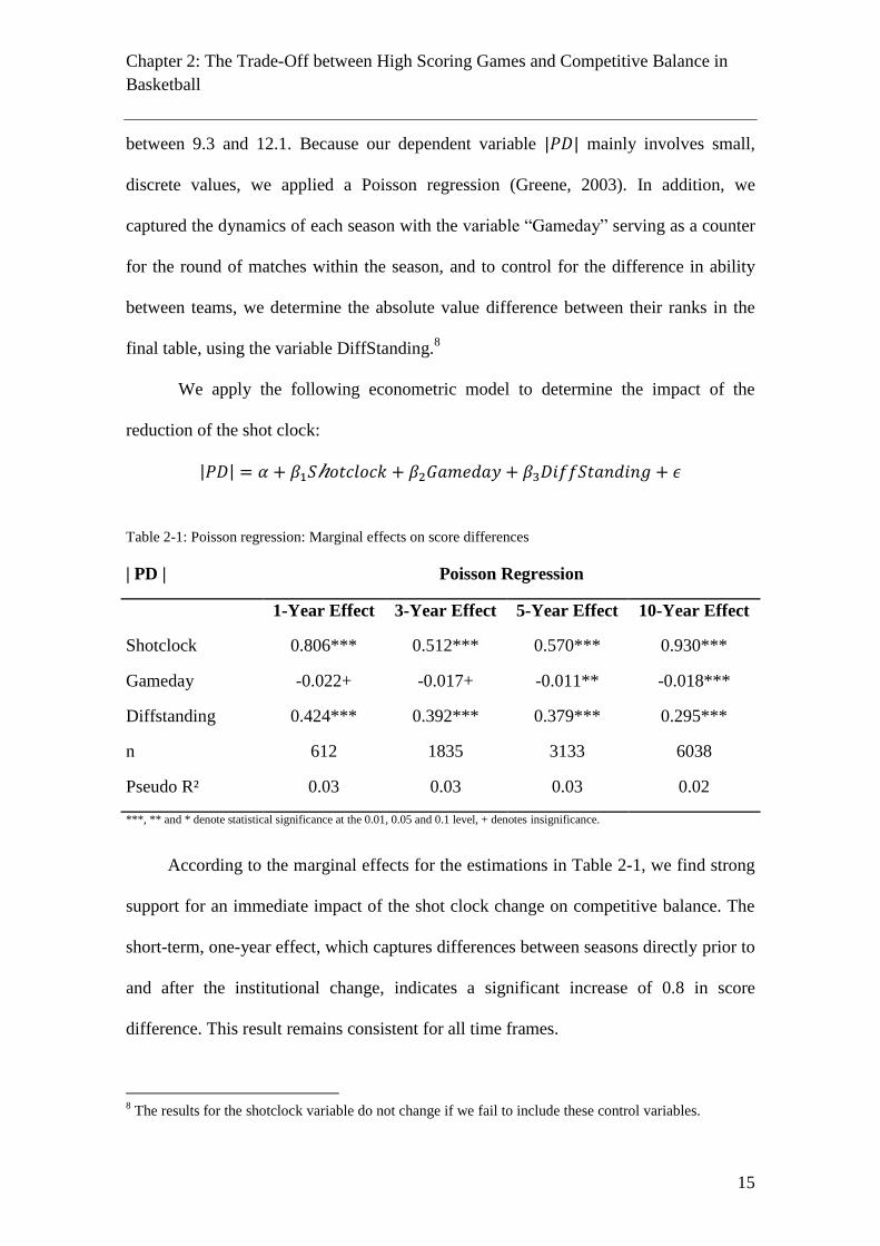
Table 2-1: Poisson regression: Marginal effects on score differences
| PD | Poisson Regression
1-Year Effect 3-Year Effect 5-Year Effect 10-Year Effect
Shotclock 0.806*** 0.512*** 0.570*** 0.930***
Gameday -0.022+ -0.017+ -0.011** -0.018***
Diffstanding 0.424*** 0.392*** 0.379*** 0.295***
n 612 1835 3133 6038
Pseudo R² 0.03 0.03 0.03 0.02
***, ** and * denote statistical significance at the 0.01, 0.05 and 0.1 level, + denotes insignificance.
According to the marginal effects for the estimations in Table 2-1, we find strong
support for an immediate impact of the shot clock change on competitive balance. The
short-term, one-year effect, which captures differences between seasons directly prior to
and after the institutional change, indicates a significant increase of 0.8 in score
difference. This result remains consistent for all time frames.
8 The results for the shotclock variable do not change if we fail to include these control variables.

Chapter 2: The Trade-Off between High Scoring Games and Competitive Balance in
Basketball
16
To measure the impact of the change on scoring, we ran a second regression to
determine the drivers of points scored during a game (Total points):
𝑇𝑜𝑡𝑎𝑙 𝑃𝑜𝑖𝑛𝑡𝑠 = 𝛼 + 𝛽1𝑆ℎ𝑜𝑡𝑐𝑙𝑜𝑐𝑘 + 𝛽2𝐺𝑎𝑚𝑒𝑑𝑎𝑦 + 𝛽3𝐷𝑖𝑓𝑓𝑆𝑡𝑎𝑛𝑑𝑖𝑛𝑔 + 𝛽4𝑆𝑒𝑎𝑠𝑜𝑛
+ 𝜖
The marginal effects for these estimations in Table 2-2 again confirm our
predictions: The reduction of the shot clock led to an increase in the number of points
scored. In the first season after the rule change the influence was especially noticeable,
with an increase of 14 points per game. The long-term effects are less convincing but
might reflect other factors that emerged over this long period. For example, basketball
underwent a development toward greater professionalization during this time, which
had effects on the league that are difficult to capture with other control variables.
In both models the mean and the variance are approximately equal neglecting a
potential problem from overdispersion in the empirical model.
Table 2-2: Poisson regression: Marginal effects on total points scored
| Totalpoints | Poisson Regression
1-Year Effect 3-Year Effect 5-Year Effect 10-Year Effect
Shotclock 14.62*** 6.30*** 2.31*** -0.908+
Gameday -0.033+ -0.000+ -0.057** -0.081+
Diffstanding 0.156+ 0.211*** 0.113*** 0.067*
n 612 1835 3133 6038
Pseudo R² 0.04 0.01 0.01 0.00
***, ** and * denote statistical significance at the 0.01, 0.05 and 0.1 level, + denotes insignificance.

Chapter 2: The Trade-Off between High Scoring Games and Competitive Balance in
Basketball
17
2.3.3 Season-Level Measures
At this level, the metrics we use to measure competitive balance reflect the final
standings, including indices such as the Gini coefficient and Herfindahl-Hirschman
index, as well as deviations in the win percentages. In addition, we consider two
dimensions of competitive balance, related to the relative strength of teams in any given
season (intra-seasonal balance) or over time (inter-seasonal balance). The most widely
applied measure is the ratio of standard deviations (RSD), which controls for both
season length and the number of teams (Fort, 2007). The RSD compares the actual
standard deviation (ASD) of win percentages against the idealized standard deviation
(ISD). Therefore, we compute RSD for a given season t as:
𝑅𝑆𝐷 = 𝐴𝑆𝐷
𝐼𝑆𝐷
where:
𝑅𝑆𝐷 =√∑
(𝑊𝑃𝐺𝑖,𝑡 − 0.5)²𝑁
𝑁𝑖=1
0.5
√𝑁
Will N being the number of games each team plays per season, and .5 the win
probability for any match in which both teams are equally strong. Greater competitive
balance is indicated if the RSD value is lower. Using the final league tables, we measure
the average win margin and points scored per match, to control for their effects on game
attractiveness, and present the results in Table 2-3.

Chapter 2: The Trade-Off between High Scoring Games and Competitive Balance in
Basketball
18
Table 2-3: Season-level measures of the effects of shot clock rule changes
Short-Term-Effects Mid-Term Effects Long-Term Effects
Season 1-Year Effect 3-Year Effect 5-Year Effect 10-Year Effect
t - 1 t + 1 in% t - 3 t + 3 in% t - 5 t + 5 in% t - 10 t + 10 in%
Totalpoints
per match 145 160 10% 154 160 4% 158 160 2% 159 157 -1%
Win
margin
per match 4.04 5.68 41% 4.18 4.99 20% 4.25 4.72 11% 4.00 4.63 16%
Ratio of
standard
deviation
1.64 2.31 40% 1.87 2.13 14% 1.95 2.01 3% 1.84 2.00 9%
Immediately after the shot clock reduction, the points per match and win margins
rose significantly, by 10% and 41%, respectively. Simultaneously, the competitive
imbalance increased by 40%, though the effects diminished over subsequent seasons.
These results affirm that an increase in game speed, and thus game attractiveness, is
accompanied by a decline in competitive balance, which supports the predicted trade-off
between these two outcomes. The contrasting long-term effects might reflect additional
rule changes such as the change of the back-pass rule and the stricter interpretation of
unsportsmanlike fouls implemented in 2008; the effect of the shot clock change cannot
be separated precisely from other, potentially contrary effects.
2.4 Discussion and Conclusion
2.4.1 Limitations
The estimation results offer convincing evidence of a trade-off between scoring
and competitive balance, but the impacts on consumer demand can be derived only by
relying on previous findings (Szymanski, 2001; Lee & Fort, 2008), because we do not
have attendance data for the period we studied. In addition, many studies adopt betting

Chapter 2: The Trade-Off between High Scoring Games and Competitive Balance in
Basketball
19
odds to determine the competitive balance of each game (Deutscher et al., 2013; Berger
& Nieken, 2014), with an assumption about the efficiency of betting markets (Fama,
1970; Levitt, 2004), which emerge as valid predictors of actual winning probabilities.
Unfortunately, historic betting odds are unavailable.
2.4.2 Implications
This study has demonstrated a trade-off between high scoring games and
competitive balance in professional basketball in Spain. Both game- and season-level
data support the prediction that the reduction of the shot clock increased scoring but
also decreased competitive balance.
The results of the empirical analysis suggest some straightforward policy
implications: If a sport’s governing body is tempted to increase the speed of the games,
it faces a significant drawback, namely, fewer surprising outcomes and less competitive
balance. Whereas major U.S. leagues already use instruments such as a rookie draft,
salary caps, and revenue sharing, our findings suggest that these procedures are neither
limitless nor necessarily successful (Szymanski & Kesenne, 2004). In the worst case
scenario, they create incentives for teams to lose games intentionally, in pursuit of better
chances of winning more games in subsequent seasons (Taylor & Trogdon, 2002;
Soebbing, Humphreys, & Mason, 2013). In Europe, the results are even more
noticeable. Its open league system, with promotion and relegation factors, creates a
higher hurdle to new rules and regulations, which would affect a large number of clubs.
Basketball is not the only sport that has adjusted its rules to increase the sport’s
appeal. For example, table tennis increased the required number of sets to win but
simultaneously reduced the number of points needed to win a set in 2001. In 1999,

Chapter 2: The Trade-Off between High Scoring Games and Competitive Balance in
Basketball
20
volleyball revised its counting rules. Demand for these sports arguably is lower than
that for basketball; it would be interesting for further research to investigate the extent
to which these sports experienced effects similar to those that we have outlined here.
Additional research also could investigate another potential positive outcome of
the rule change. That is, sports participation might shift due to rule changes that
encourage faster, more entertaining games. To test this prediction, researchers could
solicit pertinent data from sport federations linked to the development of active
members.

Chapter 3: Did the 2005 Collective Bargaining Agreement Really Improve Team
Efficiency in the NHL?
21
3 Did the 2005 Collective Bargaining Agreement Really Improve
Team Efficiency in the NHL?
3.1 Introduction
At the end of the 2003-04 season, the National Hockey League (NHL) faced
serious financial challenges. Player salaries consumed more than 65% of the generated
revenues. Hence, more than 20 of the 30 teams were claiming monetary losses. Small
market teams in particular suffered from the steady increase in player salaries; they
were unable to compete with big market teams for top players and their generous player
contracts. In addition, attendance figures decreased to a 4-year low. Consequently, top
free agents were signed by teams with large revenue streams, many of which were
located in big markets. There was no new agreement between the team owners and the
National Hockey League Players’ Association (NHLPA) in sight when the 1995
collective bargaining agreement (CBA) expired. Team owners demanded cost certainty
for their teams, whereas the NHLPA initially refused to accept salary restrictions in
terms of a salary cap. Subsequently, a novelty in hockey sport history occurred when
the team owners announced a lockout and eventually cancelled the entire 2004-05
season. A new agreement was reached in July 2005 and contained several novelties,
including a hard payroll cap as well as a revenue sharing plan. The ultimate goal of
these measures was to restore financial competitiveness, which as it is proposed, should
a priori help financially weak teams to be more competitive. In detail, the CBA includes
a salary cap as well as a salary floor. Also, the revenue sharing plan is intended to allow
low revenue teams to be more financially competitive. In order to do this, the top ten

Chapter 3: Did the 2005 Collective Bargaining Agreement Really Improve Team
Efficiency in the NHL?
22
teams contribute money to a pool where a minimum of 4.5% of league revenues are to
be distributed among the bottom 15 teams.
In order to analyze the financial situation of NHL teams before and after the CBA,
and to measure the impact of the CBA, this chapter applies stochastic frontier analysis
(SFA). The objective is to provide empirical evidence on whether or not the new CBA
did indeed improve financial competitiveness. These impacts of an institutional change
can be best observed by analyzing the team efficiency. The methodology has been
widely used in the field of sports economics. The most popular choice of output
indicators used in the existing literature has been the sporting performance (measured as
wins), winning percentage, or points achieved in a given season. For European soccer,
Dawson, Dobson, and Gerrard (2000) applied SFA to estimate the efficiency of
managers in English professional soccer. In addition, Frick and Simmons (2008) used
SFA to measure the effect of variations in managerial compensation on team success in
the German Bundesliga. Barros and colleagues (Barros, Del Corral, & Garcia-del-
Barrio, 2008; Barros, Garcia-del-Barrio, & Leach, 2009) analyzed technical efficiency
of football clubs in the Spanish Primera Division as well as in the English Premier
League with a random frontier model. Concerning U.S. team sport franchises Zak,
Huang, and Siegfried (1979) were the first to analyze efficiencies of 5 NBA teams with
a Cobb-Douglas deterministic frontier model. Hofler and Payne (1997) extended this
approach and examined a cross-sectional analysis of all 27 NBA teams for the 1992-93
season in order to observe if teams play up to their potential in terms of actual wins. In a
subsequent study, Hofler and Payne (2006) used panel data for the stochastic production
frontier model.
Chapter 3: Did the 2005 Collective Bargaining Agreement Really Improve Team
Efficiency in the NHL?
23
In a different strand of literature, Kahane (2005) applied SFA for the NHL and
identifies technical inefficiency in production. His results indicate that franchises owned
by corporations tend to be more efficient than franchises owned by individuals, and
teams with a greater relative presence of French-Canadian players tended to be less
efficient. In a similar direction, Fort, Lee, and Berri (2008) applied SFA to address the
issue on discrimination in retention of NBA coaches and detected no difference in
technical efficiency by race of the coach.
Because team owners postulated over ways to reach cost certainty through the
2005 NHL CBA, it seems to be obvious that team owners are not solely interested in
success on the ice and the glory of victory. From the team owners´ perspective, it is
imperative that the franchise achieves a positive return of their investment. The present
study explores the relationship between the 2005 NHL CBA and financial success of
franchise teams relative to their potential. By using team values, as well as franchises´
revenues, as outputs to measure technical efficiencies, the study focuses on economic
efficiency. Previous studies, as shown above, predominantly used sporting performance
as the output variable for measuring team success. But a sport, even though advocated
differently on a regular basis, is not just about winning games. The franchise system of
the NHL-which, as stated above, struggled heavily right before the lockout-has to make
sure that teams operate efficiently, in terms of financial performance, to ensure the
future of the league. Because of this, we deviate from the existing literature by
introducing financially important outcome variables.
One method has been ignored in the literature so far: using team values as well as
revenues as outputs for measuring technical efficiencies. Thus, the current research is
Chapter 3: Did the 2005 Collective Bargaining Agreement Really Improve Team
Efficiency in the NHL?
24
innovative in this context. Efficiency can also be used as a direct benchmark between
franchises operating in the same institutional environment. Our article closes this gap
through the analysis of the impact of the new CBA on efficiency; specifically, team
value maximization and value generation of low performing teams immediately
increased efficiencies after the lockout.
3.2 Data Description
The data set we used includes information on the four seasons prior to the lockout,
from 2000-01 to 2003-04, and the four seasons immediately following the lockout, from
2005-06 to 2008-09. At the beginning of the 2000-01 season, the NHL expanded from
28 to 30 teams as the Minnesota Wild and the Columbus Blue Jackets joined the league.
Because we took the previous season into account, the resulting (unbalanced) panel data
set contained 238 observations on all variables included in the estimates.
Frontier models require identifying inputs and outputs. In order to determine how
efficiently the franchises operated, it was essential for us to use a financial ratio as the
output. Forbes magazine reports data annually on sport franchise´s team values, as well
as revenues for all major leagues. It breaks down franchise valuation into four
categories: sport, market, stadium, and brand management. Team value has been
previously applied as a dependent variable to analyze determinants of franchise values
(Alexander & Kern 2004; Humphreys & Mondello, 2008). Therefore, as franchise
values are not equally distributed, this study applied the natural logarithm of team
values as output. Furthermore, to ensure the robustness of our results, we used the
natural logarithm of revenues for each franchise as a second output. This data is also
published by Forbes magazine on a yearly basis.
Chapter 3: Did the 2005 Collective Bargaining Agreement Really Improve Team
Efficiency in the NHL?
25
The input variables represented the various factors that were most likely to
determine a team´s franchise value. Therefore, we included the natural logarithm of the
population of each team´s metropolitan area in order to account for market-size effects
on franchise values. In metropolitan areas with more than one NHL franchise (e.g., Los
Angeles and New York), each franchise was credited with the entire population in the
metropolitan area—this is because the market cannot be unambiguously separated
between each franchise. Data were obtained from the U.S. Bureau of Economic
Analysis´ Regional Economic Accounts and Statistics, Canada. Since franchises share
larger pools of potential fans, we expected a positive relationship between teams located
in larger markets and franchise values as well as revenues. It should be noted that,
unlike in European soccer, only very few fans join their favorite teams for road games.
This is due in part to a greater number of games and a lengthier distance between
competing teams.
The team´s stadium is another important input factor for multiple reasons. A
franchise with a new stadium can expect higher revenues, and hence higher team values
due to e.g. state-of-the-art luxury boxes, for example. Alexander and Kern (2004) and
Miller (2007) identified that new sport stadiums experience a honeymoon effect, where
attendees visit the stadium for the stadium and not necessarily to watch the team, which
lasts between 6 to 10 years after inauguration. Hence, we included stadium age, as well
as stadium age in quadratic form, in our analysis and expected a negative impact of
arena age and an increase in marginal returns on both dependent variables. Data on
arena age was collected from Munsey and Suppes´ website (http://www.ballparks.com).
In addition, the natural logarithm of attendees per game was included. We assumed that,
since each attendee generates revenues for the franchise, the higher the number of

Chapter 3: Did the 2005 Collective Bargaining Agreement Really Improve Team
Efficiency in the NHL?
26
attendees, the greater the team value. To measure this revenue stream, we used the team
marketing annual reports from the Fan Cost Index (FCI), which are constructed for each
franchise and year.9 The FCI tracks the cost of attending a sporting event for a family of
four.10
The more a franchise is able to charge for their tickets and other amenities, the
more revenues it generates. Thus, we presumed that the coefficient for the FCI would
also be positively related to the team value. To analyze how franchise history affects
team value, we included the duration of a team in the league and the squared duration of
a team in the league. We expect that teams with a longer franchise history also report a
higher team value.11
We also control for the athletic achievements of a team. Since NHL standings are
based on points and not wins, the rank is not expressed in terms of winning percentages;
this is because teams receive a point for an overtime loss. We estimated athletic
achievement by dividing the team´s total in the previous season by the average points of
all teams in the previous season. Following the approach by Miller (2007), points
achieved in the previous season are considered to be an important component in
determining ticket prices, season ticket sales, media revenues, and advertising prices.
We expected a positive coefficient, suggesting that a better athletic achievement in the
previous season leads to higher revenues and, therefore, a higher franchise value. One of
the most important input factors in professional sports is team expenses. We measure
these by including the natural logarithm of the team payroll in our analysis. Data were
drawn from USA Today
9 Information is available at Rodney Fort’s website at http://www.rodneyfort.com.
10 The FCI comprises the prices of four average-price tickets, two small draft beers, four small soft drinks,
four regular-size hot dogs, parking for one car, two game programs and two least-expensive, adult-size
adjustable caps. 11
We did not include the natural logarithm of the input variables Duration and Age Arena since the value
of 0 is not defined.

Chapter 3: Did the 2005 Collective Bargaining Agreement Really Improve Team
Efficiency in the NHL?
27
(http://content.usatoday.com/sports/hockey/nhl/salaries/default.aspx). We assumed that
a team with high payroll expenses will offer a superior team quality and, therefore,
provides a superior utility to fans. Due to this assumption, we anticipated that higher
team expenses would positively influence the team´s value. All monetary magnitudes in
this analysis (e.g., team value, FCI, payroll) were deflated by the Consumer Price Index
(CPI), which was taken from U.S. Bureau of Labor Statistics, and expressed at prices
for the year 2000. Descriptive statistics for all variables introduced above are shown in
Table 3-1.
Table 3-1: Descriptive Statistics of indicators influencing team values
Variable Operationalization Mean Min. Max.
Log Value Natural log of the team value in Dollar 18.88 18.18 19.78
Log Population Natural log of metropolitan area population 15.13 13.64 16.76
Age Arena Tenure of the team in the arena 12.38 0 47
Age Arena² Squared tenure of the team in the arena 270.0 0 2209
Duration Duration of the team in the league 34.45 0 99
Duration² Squared duration of the team in the league 1,964 0 9,801
Relative Points Achieved points in previous season/average
points 1 0.45 1.37
Log Attendance Natural log of attendance 9.72 9.18 9.97
Log FCI Natural log of fan cost index 5.46 4.98 5.98
Log Pay Natural log of team payroll 17.40 16.28 18.11
3.3 Empirical Analyses of Efficiencies
We applied a stochastic production frontier model to explore whether the new
CBA did indeed improve technical efficiencies among the teams in the league. In the
present study, the output of the teams in the NHL was measured by the team values as
Chapter 3: Did the 2005 Collective Bargaining Agreement Really Improve Team
Efficiency in the NHL?
28
well as revenues after the respective season. To compute technical efficiencies, we
applied the model introduced by Battese and Coelli (1995), which allows for time-
varying efficiencies. It assumes a log-linear production function for a set of 𝑖 firms over
𝑡 time-periods and can be expressed as follows:12
𝑦𝑖𝑡 = 𝑥𝑖𝑡𝛽 + (𝑣𝑖𝑡 − 𝑢𝑖𝑡),
𝑖 = 1, … , 𝑁 and 𝑡 = 1, … , 𝑇, (1)
Where 𝑦𝑖𝑡 is the natural logarithm of the franchise value, 𝑥𝑖𝑡 is a vector of team-specific
input quantities, and 𝛽 is a vector of unknown coefficients over which the likelihood
will be maximized. Furthermore, 𝑣𝑖𝑡 represents a random error term that is assumed to
be independent and identically distributed (i.i.d.) 𝑁(0, 𝜎𝑣2). 𝑢𝑖𝑡 is i.i.d. and a non-
negative random error term that accounts for technical inefficiency in production, and is
further assumed to follow a normal distribution truncated at zero of the 𝑁(𝑚𝑖𝑡, 𝜎𝑢2)
distribution. 𝑚𝑖𝑡 is given as
𝑚𝑖𝑡 = 𝑧𝑖𝑡𝜎, (2)
𝑧𝑖𝑡 is a vector of variables that may influence the efficiency as team value creation, and
is a vector to be estimated. Using data from the NHL from 2000-01 to 2008-09, we
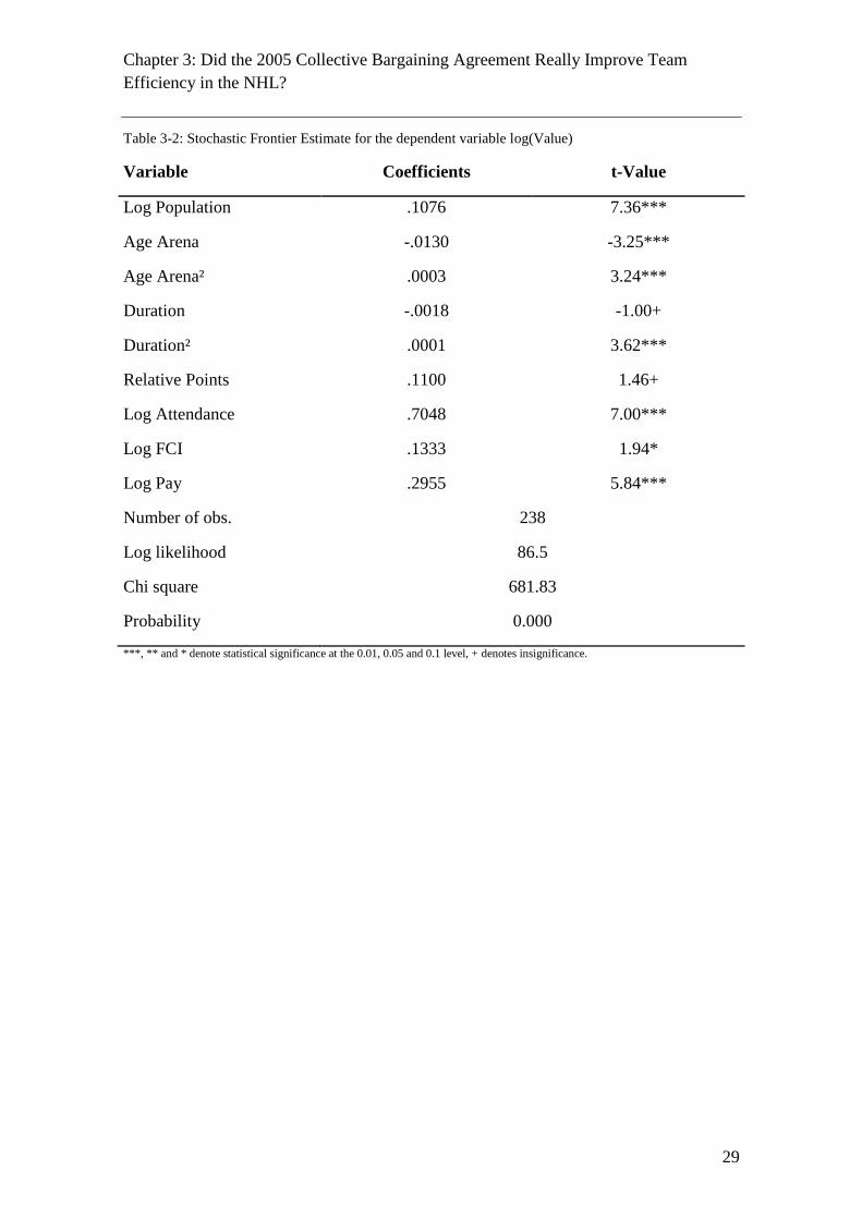
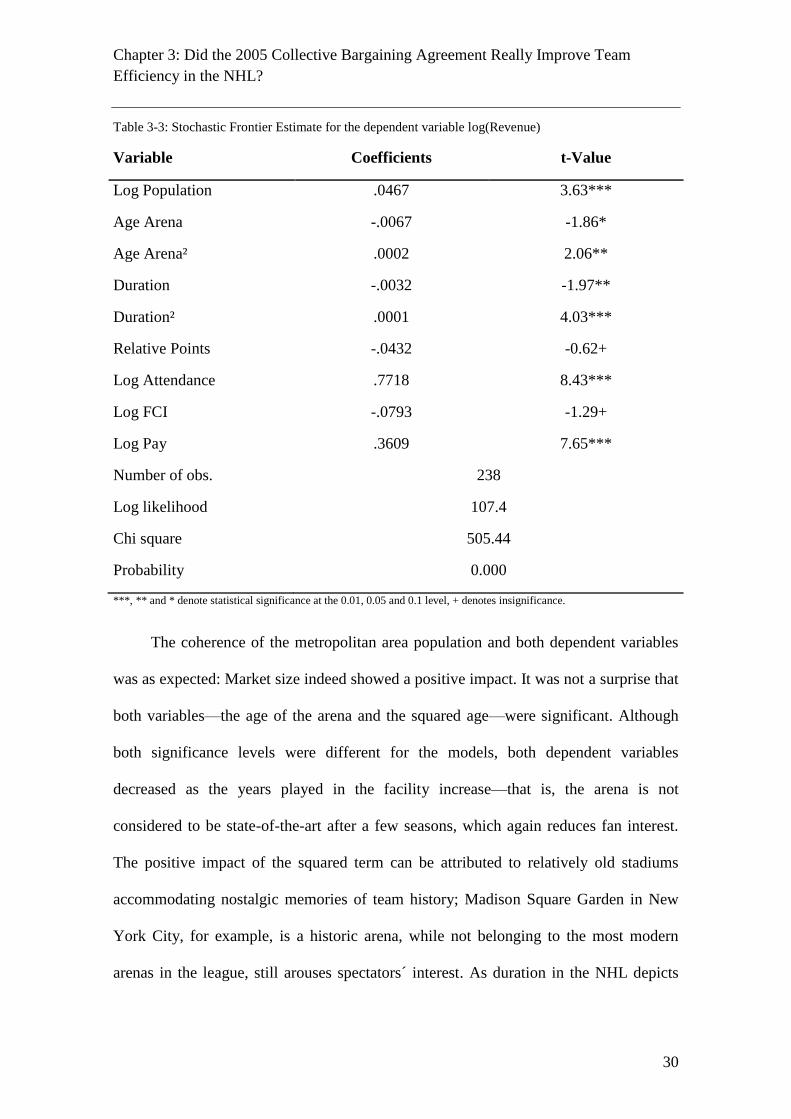
accomplished a total of 238 observations for 30 teams. Table 3-2 presents the maximum
likelihood estimate for our frontier model for franchise values, while Table 3-3 presents
results for revenue generation. All results are robust and not vulnerable to either
multicollinearity or heteroskedasticity.
12
The applied software for the frontier analysis is Stata11 SE.
Chapter 3: Did the 2005 Collective Bargaining Agreement Really Improve Team
Efficiency in the NHL?
29
Table 3-2: Stochastic Frontier Estimate for the dependent variable log(Value)
Variable Coefficients t-Value
Log Population .1076 7.36***
Age Arena -.0130 -3.25***
Age Arena² .0003 3.24***
Duration -.0018 -1.00+
Duration² .0001 3.62***
Relative Points .1100 1.46+
Log Attendance .7048 7.00***
Log FCI .1333 1.94*
Log Pay .2955 5.84***
Number of obs. 238
Log likelihood 86.5
Chi square 681.83
Probability 0.000
***, ** and * denote statistical significance at the 0.01, 0.05 and 0.1 level, + denotes insignificance.
Chapter 3: Did the 2005 Collective Bargaining Agreement Really Improve Team
Efficiency in the NHL?
30
Table 3-3: Stochastic Frontier Estimate for the dependent variable log(Revenue)
Variable Coefficients t-Value
Log Population .0467 3.63***
Age Arena -.0067 -1.86*
Age Arena² .0002 2.06**
Duration -.0032 -1.97**
Duration² .0001 4.03***
Relative Points -.0432 -0.62+
Log Attendance .7718 8.43***
Log FCI -.0793 -1.29+
Log Pay .3609 7.65***
Number of obs. 238
Log likelihood 107.4
Chi square 505.44
Probability 0.000
***, ** and * denote statistical significance at the 0.01, 0.05 and 0.1 level, + denotes insignificance.
The coherence of the metropolitan area population and both dependent variables
was as expected: Market size indeed showed a positive impact. It was not a surprise that
both variables—the age of the arena and the squared age—were significant. Although
both significance levels were different for the models, both dependent variables
decreased as the years played in the facility increase—that is, the arena is not
considered to be state-of-the-art after a few seasons, which again reduces fan interest.
The positive impact of the squared term can be attributed to relatively old stadiums
accommodating nostalgic memories of team history; Madison Square Garden in New
York City, for example, is a historic arena, while not belonging to the most modern
arenas in the league, still arouses spectators´ interest. As duration in the NHL depicts

Chapter 3: Did the 2005 Collective Bargaining Agreement Really Improve Team
Efficiency in the NHL?
31
the tradition of a team, only the squared term significantly impacted both dependent
variables. This can be explained by team tradition, which cannot be established within a
short period of time. The negative effect of duration on the nonquadratic term can be
explained by the honeymoon effect, which diminished after the inauguration.13
Although these indicators of arena and team history had the expected impact, sporting
performance in the previous season apparently has not—that is, it did not impact team
value or revenues in a significant way. In our model, both indicators for match day
revenues affected our dependent variables in a positive way: Average attendance and
the FCI exhibit statistically significant impacts. Finally, the team payroll-depicting team
quality and serving as an indicator for the asset the squad displays—has the expected
positive impact on both team values and revenue.
After providing insights on indicators influencing team values in the NHL, and
establishing a basis for calculating efficiencies for each team and each season, we
pursued the initial inquiry to determine whether the lockout in 2004-05 improved these
efficiencies.
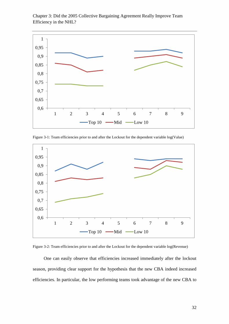
Figure 3-1 and Figure 3-2 provide information on the average efficiencies for a
particular season on the 10 most efficient teams, the 10 least efficient teams, and the 8-
10 teams in between.
13
The honeymoon effect is an increase in attendance after the opening of a new facility which fades after
some time. For literature in major league sports see for example Leadley & Zygmont (2005, 2006) or
Scully (1989).
Chapter 3: Did the 2005 Collective Bargaining Agreement Really Improve Team
Efficiency in the NHL?
32
Figure 3-1: Team efficiencies prior to and after the Lockout for the dependent variable log(Value)
Figure 3-2: Team efficiencies prior to and after the Lockout for the dependent variable log(Revenue)
One can easily observe that efficiencies increased immediately after the lockout
season, providing clear support for the hypothesis that the new CBA indeed increased
efficiencies. In particular, the low performing teams took advantage of the new CBA to
0,6
0,65
0,7
0,75
0,8
0,85
0,9
0,95
1
1 2 3 4 5 6 7 8 9
Top 10 Mid Low 10
0,6
0,65
0,7
0,75
0,8
0,85
0,9
0,95
1
1 2 3 4 5 6 7 8 9
Top 10 Mid Low 10
Chapter 3: Did the 2005 Collective Bargaining Agreement Really Improve Team
Efficiency in the NHL?
33
close the gap to the high performing teams. This is true for both models, as average
efficiency for the 10 least efficient teams improved from 0.73 to 0.84 for Model 1, and
from 0.72 to 0.86 for Model 2. Once the new CBA was established, average efficiencies
leveled off around 7% higher than before the lockout for Model 1 and approximately
9% higher than before the lockout for Model 2. The expectation stated in the
introduction, which claims a strengthened competitiveness due to the new CBA, was
supported by our estimations.
3.4 Conclusions
This chapter has investigated the impact of the new CBA on efficiencies
concerning maximizing team values as well as revenue generation. After the lockout
season in 2004, we observed an abrupt increase in technical efficiencies after the new
collective bargaining agreement was installed—particularly concerning low performing
teams benefitting from salary restrictions and revenue sharing.
As our study is the first to use team values and revenues in connection with
measuring technical efficiencies of teams, several follow-up questions arise: For
example, it would be of great interest to explore if team efficiencies benefit or suffer
from having another major league team in the city; in other words, analyzing whether a
tougher competition in a local market would serve as a catalyzer and lead to an increase
in managerial performance. Going into more detail, it would be interesting to see if
certain combinations of teams from the major league teams could serve as substitutes or
complements. As our analysis provides a somewhat surprising result that sporting
performance neither influences team values nor team revenues, future research could
compare other major leagues to examine its potential influence in other sports.

Chapter 4: Sport or Business Approach? A Cross-Continent Analysis of U.S. Major
League Franchises and English Premier League Clubs
34
4 Sport or Business Approach? A Cross-Continent Analysis of U.S.
Major League Franchises and English Premier League Clubs
4.1 Introduction
The question of which primary objectives drive professional sport teams has long
been controversial among sports economists. A popular strand of predominately U.S.
literature adopts the profit maximisation hypothesis, such as in early theoretical models
by Rottenberg (1956) and Neale (1964) that regard individual teams or leagues as firms
that seek to increase their profits (see also El-Hodiri & Quirk, 1971; Fort & Quirk,
1995; Falconieri, Palomino, & Sákovics, 2004). In contrast, Sloane (1971) provides one
of the earliest arguments that European clubs favor wins rather than profits (Rascher,
1997; Késsene, 1999, 2000, 2006; Zimbalist, 2003; Vrooman, 2007). These descriptions
have prompted a broad classification, by which North American team owners are profit-
maximising business people, whereas European team owners are said to be sportsmen
and -women (Fort, 2000; Cain & Haddock, 2005). Rather than maximise profits, the
sporting group sacrifices profits to win and ultimately become win maximisers who
literally seek to win at any cost (Vrooman, 2007).
A more recent hybrid argument suggests that clubs maximise a weighted sum of
profits and wins (Dietl, Grossmann, & Lang, 2011). Although two empirical studies
indicate that clubs trade off points and wins (Atkinson, Stanley, & Tschirhart, 1988;
Garcia-del-Barrio & Szymanski, 2009), empirical evidence remains scarce, and no
cross-continent empirical analysis of North American and European clubs has detailed
their distinct economic behaviours or motives contribute to clarify the debate. In
response, the current study seeks to both close the research gap and suggest a novel

Chapter 4: Sport or Business Approach? A Cross-Continent Analysis of U.S. Major
League Franchises and English Premier League Clubs
35
approach for analysing the determinants of financial performance and the technical
financial and athletic efficiency of North American major league sports and English
Premier League football (i.e., soccer) teams, using parallel data sets. Information about
nine consecutive seasons, from 2001-02 to 2009-10, covers 162 teams from North
America’s National Hockey League (NHL), National Basketball Association (NBA),
National Football League (NFL), and Major League Baseball (MLB), as well as the
English Premier League (EPL), producing a total of 1,237 team-season observations. As
measures of financial performance, this study uses Forbes’ franchise valuations for the
major league clubs and Deloitte’s Annual Review of Football Finance (Deloitte &
Touche, 2001-2009) to gather the annual revenues of the EPL clubs. In terms of
technical efficiency, this research relies on either winning percentages (NBA, NFL, and
MLB) or points per season (NHL and EPL) as a measure of athletic performance. In
turn, it offers, to the best of the author’s knowledge, the first empirical assessment of
the profit and win maximisation hypotheses that combines panel regressions with data
envelopment analysis (DEA) in a cross-continental data set.
The results reveal several distinct motives of professional sport teams. In
particular, athletic achievement exerts an effect on teams’ financial performance only
among EPL teams, not across the North American major league franchises. The
outcomes of the DEA also indicate that the motives driving the major league franchises
tend to be more business oriented, whereas the rationale for the EPL clubs is to
maximise their sporting performance.
The next section proceeds with reviews of the existing literature pertaining to the
determinants of franchise value and the use of efficiency analyses in professional sports

Chapter 4: Sport or Business Approach? A Cross-Continent Analysis of U.S. Major
League Franchises and English Premier League Clubs
36
contexts. Following a brief discussion of the applied data, this study specifies the model
and presents the results from the empirical analysis. It concludes with a discussion of
the empirical results and limitations, along with an outlook on further research.
4.2 Literature Review
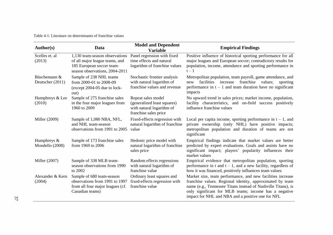
Empirical research into the value of professional sport clubs remains nascent, with
just a few exceptions. For example, Humphreys and Lee (2010) and Humphreys and
Mondello (2008) analyse franchise sale prices in the four North American Major
Leagues. Emphasising the determinants of team value and revenues, Alexander and
Kern (2004) find that the income levels and population of the local market, as well as
the presence of new facilities and a strong regional identity, influence franchise values
for major league teams. Miller (2007) studies MLB, and Miller (2009) investigates the
NBA, NFL, and NHL, to extend these approaches and include facility and franchise
age, public or private ownership, and duration of the franchise in the city. Büschemann
and Deutscher (2011) also incorporate NHL team payrolls, attendance per game, and a
fan cost index in their analysis. Scelles, Helleu, Durand, and Bonnal (2013) offer the
first comparison of the determinants of franchise values between the North American
major leagues and European soccer teams, using the aforementioned set of variables,
though they include the team values of only a subset of the 20 most valuable pan-
European teams, as published by Forbes, which suggests the potential for a selection
bias. Table 4-1 contains an overview of previous literature and the relevant empirical
findings.
37
Table 4-1: Literature on determinants of franchise values
Author(s) Data Model and Dependent
Variable Empirical Findings
Scelles et. al
(2013) 1,130 team-season observations
of all major league teams, and
185 European soccer team-
season observations, 2004-2011
Panel regression with fixed
time effects and natural
logarithm of franchise values
Positive influence of historical sporting performance for all
major leagues and European soccer; contradictory results for
population, income, attendance and sporting performance in
t – 1
Büschemann &
Deutscher (2011) Sample of 238 NHL teams
from 2000-01 to 2008-09
(except 2004-05 due to lock-
out)
Stochastic frontier analysis
with natural logarithm of
franchise values and revenue
Metropolitan population, team payroll, game attendance, and
new facilities increase franchise values; sporting
performance in t – 1 and team duration have no significant
impacts
Humphreys & Lee
(2010) Sample of 275 franchise sales
in the four major leagues from
1960 to 2009
Repeat sales model
(generalized least squares)
with natural logarithm of
franchise sales price
No upward trend in sales prices; market income, population,
facility characteristics, and on-field success positively
influence franchise values
Miller (2009) Sample of 1,080 NBA, NFL,
and NHL team-season
observations from 1991 to 2005
Fixed-effects regression with
natural logarithm of franchise
value
Local per capita income, sporting performance in t – 1, and
private ownership (only NHL) have positive impacts;
metropolitan population and duration of teams are not
significant
Humphreys &
Mondello (2008) Sample of 173 franchise sales
from 1969 to 2006 Hedonic price model with
natural logarithm of franchise
sales price
Empirical findings indicate that market values are better
predicted by expert evaluations. Goals and assists have no
significant impact; players’ popularity influences their
market values Miller (2007) Sample of 338 MLB team-
season observations from 1990
to 2002
Random effects regressions
with natural logarithm of
franchise value
Empirical evidence that metropolitan population, sporting
performance in t and t – 1, and a new facility, regardless of
how it was financed, positively influences team values
Alexander & Kern
(2004) Sample of 680 team-season
observations from 1991 to 1997
from all four major leagues (cf.
Canadian teams)
Ordinary least squares and
fixed-effects regression with
franchise value
Market size, team performance, and new facilities increase
franchise values. Regional identity, approximated by team
name (e.g., Tennessee Titans instead of Nashville Titans), is
only significant for MLB teams; income has a negative
impact for NHL and NBA and a positive one for NFL

Chapter 4: Sport or Business Approach? A Cross-Continent Analysis of U.S. Major
League Franchises and English Premier League Clubs
38
To analyse differences in the motives of owners across countries, this research
proposes a nonparametric data envelopment analysis (DEA) as a means to measure
efficiency in terms of financial and sporting performance. Prior literature features two
approaches to efficiency measures, either DEA or a parametric approach, as exemplified
by stochastic frontier analysis (SFA). The main argument in support of DEA is its
applicability even with a relatively small sample size (Barros & Leach, 2006; Jardin,
2009; Barros, Assaf & Sá-Earp, 2010). However, unlike SFA, no well-developed
statistical tests for DEA exist to validate the specifications of a particular model.
Considering though that DEA has been applied in many research fields, including
agriculture (Picazo-Tadeo, Gomez-Limon, & Reig-Martinez, 2011), environmental
economics (Roghanian & Foroughi, 2010), and public services (Alexander, Haug, &
Jaforullah, 2010), and the small sample size mandated by the EPL with its 20 teams per
season, the DEA approach seems most appropriate.
Fizel and D´Itri (1997) apply DEA to sports economics to measure the individual
efficiency of college basketball coaches. More recent applications of DEA techniques
include analyses of sporting and financial performance in European soccer leagues; for
example, Barros and Garcia-del-Barrio (2011), Picazo-Tadeo and Gonzalez-Gomez
(2010), and Guzman (2006) study the Spanish Primera División; Guzman and Morrow
(2007), Barros and Leach (2006), and Haas (2003a) investigate the EPL; Kounetas
(2013) studies the Greek Super League; Jardin (2009) focuses on the French Ligue 1;
and Espitia-Escuer and García-Cebrián (2010) address participants in the UEFA
Champions League. The primary objective of these studies was to examine sporting and
financial efficiency and provide benchmarks against peers as the summary in Table 4-2
reveals.

39
Table 4-2: Literature on data envelopment analysis in sport
Author(s) Data Applied Model Inputs Output(s)
Kounetas (2013) 14 Greek Super League
clubs from 2000 to 2008 Bootstrap DEA and
truncated regression Transfer expenses, contract renewals,
operational costs, profits, age, location,
and goal ratio
Points and attendance
Barros & Garcia-del-
Barrio (2011) 12 Primera Division
clubs, from 1996-97 to
2003-04
Bootstrap DEA and
truncated regression Operational costs, team payroll, and
total assets Attendance and other receipts
Barros et al. (2010) 20 Brazilian football
clubs from 2006 to 2007 Bootstrap DEA and
truncated regression Operational costs, team payroll and
total assets Attendance and other receipts
Espitia-Escuer & García-
Cebrián (2010) 32 teams per season in
Champions League from
2003 to 2007
Modified DEA, version
by Anderson & Peterson
(1993)
Attacking plays, squad size, and ball
possession Goal attempts and number of
appearances in UEFA
Champions League
Picazo-Tadeo &
Gonzalez-Gomez (2010) 20 Primera Division
football teams per
season from 2001–02 to
2007–08
DEA Squad size, duration in national first
division, and attendance Points
Jardin (2009) 14 Ligue 1 football clubs
from 2004-05 to 2006-
07
DEA Payroll and metropolitan population Points and turnovers
Guzman & Morrow
(2007) 115 EPL team-season
obervations from 1997-
98 to 2002-03
DEA with canonical
correlation analysis Team payroll and director’s
remuneration Points and total revenue
Barros & Leach (2006) 12 EPL teams from
1998-99 to 2002-03 DEA Squad size, payroll, net assets, and
stadium facilities expenditure Points, attendance, and
turnover Guzman (2006) 14 Primera Division
teams from 2000-01 to
2002-03
DEA and Malmquist
productivity index Payroll and general expenses Turnover
Haas (2003a) 20 EPL teams for the
season (2000-01) DEA Payroll, coach salary, and metropolitan
population Points, attendance, and
revenue Haas (2003b) 12 Major League Soccer
teams in 2000 DEA Payroll, coach salary, and capacity
utilization Points, attendance, and
revenue
Chapter 4: Sport or Business Approach? A Cross-Continent Analysis of U.S. Major
League Franchises and English Premier League Clubs
40
Somewhat surprisingly, analyses of the financial efficiency of North American
sport leagues remain rare, with the exceptions of Haas (2003b, Major League Soccer)
and Büschemann and Deutscher (2011, NHL). Instead, most of these studies focus on
the efficiency of sporting performance, measured as winning percentage or points in a
given season (Porter & Scully, 1982; Scully, 1994; Hadley, Poitras, Ruggiero, &
Knowles, 2000; Einolf, 2004; Hofler & Payne, 2006; Lewis, Sexton, & Lock, 2007). No
research addresses cross-continent comparisons.
4.3 Data set and Descriptive Statistics
The analysed data set contains information about nine seasons of four North
American major league franchises and all teams participating in the EPL, though the
data for the NHL only span eight seasons, due to the 2004-05 lock-out. In total, 32
NBA, 32 NFL, 30 NHL, 31 MLB, and 37 EPL teams appear in the data set, yielding for
1,237 team-season observations. During the observed period, four franchises relocated
permanently (Montreal Expos, Vancouver Grizzlies, Charlotte Hornets, and Seattle
Supersonics) and thus were treated as new observations, because the franchises began
operating in a different market and played in new facilities. The analysis of the
determinants of financial performance required the use of a financial ratio as the
dependent variable. Forbes magazine provides sport franchises’ annual team values for
all major leagues, departed into four categories: sport, market, stadium, and brand
management. It recently has begun to publish team values for European soccer clubs
too, but it includes only the 25 most valuable European teams and does not specify
valuations for particular leagues. Because of this data constraint, the current study relies
on revenues, instead of franchise values, for EPL clubs. Vine (2004) and Fort (2006)
further argue that the Forbes values generally represent a simple multiple of revenues
Chapter 4: Sport or Business Approach? A Cross-Continent Analysis of U.S. Major
League Franchises and English Premier League Clubs
41
by some factor, between 3 and 5.5, so the results should be comparable across the
different analysis methods. The EPL data were available in Deloitte’s Annual Review of
Football Finance (Deloitte & Touche, 2001-2009). Because franchise values and
revenues are not normally distributed, this study applies the natural logarithm of team
values and revenues.
The explanatory variables represent various factors that prior studies have
suggested are likely determinants of franchise values and revenues. The natural
logarithm of the standard metropolitan statistical area (SMSA) population and SMSA
per capita income both control for market size effects. Teams located in larger, possibly
wealthier markets have access to a larger pool of potential fans and thus enjoy
favourable positions in terms of negotiating more lucrative cable television contracts or
increasing gate receipts and game-day revenues. In metropolitan areas with more than
one team (e.g., Los Angeles, New York, London), the entire population in the
metropolitan area gets assigned to each team, because it is impossible to unambiguously
separate the market across the multiple teams. Ultimately, a positive relationship is
likely among population, income, and team values (Alexander & Kern, 2004; Miller,
2009; Scelles et al., 2013). The major league data came from the U.S. Bureau of
Economic Analysis, which produces Regional Economic Accounts, and Statistics
Canada; the EPL data came from the Office for National Statistics.
Team stadiums also constitute important factors. A team with a new stadium can
expect higher revenues, from the sale of luxury suites and enhanced concession
revenues (Miller, 2007; Scelles et al., 2013). Therefore, facility age should have a
negative sign indicating a positive effect of new opened arenas on team values; the

Chapter 4: Sport or Business Approach? A Cross-Continent Analysis of U.S. Major
League Franchises and English Premier League Clubs
42
relevant data came from http://www.stadiumguide.com and http://www.ballparks.com.
Another age variable, namely, the duration of a team in the league, accounts for how
team history affects team values. A relegation and promotion system exists only in
European football, so for the EPL teams, this study uses total duration in the first
division. In general though, teams with a longer team history should report higher team
values.
In addition, by including the natural logarithm of attendees per game, this study
acknowledges that more attendees should increase team value, because each attendee
generates revenue. Attendance relates to but is distinct from another potentially
influential variable, namely, sporting performance in the previous season (Alexander &
Kern; 2004; Miller, 2007). This performance influences ticket prices, season ticket
sales, media revenues, and advertising prices. The measure of performance reflects the
athletic achievements of the entire team; Winning percentage is included to control for
this effect. NHL and EPL standings are based on points, not wins (e.g., a team gains a
point for an overtime loss in the NHL or for a draw in EPL), so for these leagues,
sporting performance equals the ratio of points achieved by the team in the previous
season, divided by the average points of all teams in the previous season. The effect of a
strong performance in the previous season on franchise values and team revenues
should be greater for win-maximising teams (EPL) than for revenue-maximising teams
(all other teams).
The salaries paid to players average at least 50% of total team expenses and are
therefore a key determinant and potential differentiating factor. Including the natural
logarithm of the team payroll in the analysis reflects the assumption that higher

Chapter 4: Sport or Business Approach? A Cross-Continent Analysis of U.S. Major
League Franchises and English Premier League Clubs
43
expenses lead to superior team quality, which has more utility for fans. That is, higher
team expenses should enhance team value. Salary data were obtained from Rodney
Fort’s Sports Business Data for all major league franchises and Deloitte’s Annual
Review of Football Finance for EPL clubs. Any monetary variables (i.e., team values,
revenues, payroll, and income) are deflated by the Consumer Price Index, taken from
the U.S. Bureau of Labor Statistics for major league teams and the U.K. Statistics
Authority for EPL teams, and normalised to their level in the year 2000 (2000 = 100).
The descriptive statistics for all these variables are presented in Table 4-3.

44
Table 4-3: Descriptive statistics
Variable Operationalization
Mean SD Min Max Mean SD Min Max Mean SD Min Max Mean SD Min Max Mean SD Min Max
overall 8,43 0,11 8,13 8,71 8,83 0,11 8,53 9,13 8,19 0,14 7,90 8,58 8,46 0,18 7,96 9,09 7,78 0,25 6,79 8,44
between 0,10 8,20 8,66 0,07 8,74 9,03 0,13 8,03 8,46 0,17 8,04 8,94 0,22 7,13 8,27
within 0,06 8,23 8,55 0,09 8,55 8,99 0,06 8,03 8,33 0,08 8,19 8,68 0,10 7,44 8,12
overall 7,71 0,11 7,32 8,66 7,89 0,08 7,63 8,09 7,54 0,13 7,07 7,87 7,80 0,18 7,12 8,27 7,59 0,23 7,05 8,20
between 0,07 7,57 7,90 0,02 7,86 7,93 0,09 7,38 7,73 0,16 7,49 8,19 0,20 7,16 7,96
within 0,09 7,46 8,54 0,08 7,64 8,08 0,09 7,23 7,79 0,09 7,42 8,05 0,13 7,18 8,20
overall 6,58 0,34 6,00 7,28 6,49 0,35 5,46 7,28 6,57 0,38 5,92 7,28 6,65 0,28 6,18 7,28 5,85 0,68 4,82 6,92
between 0,34 6,02 7,27 0,35 5,47 7,27 0,39 6,02 7,27 0,28 6,19 7,27 0,63 4,84 6,89
within 0,02 6,50 6,62 0,02 6,40 6,54 0,03 6,47 6,75 0,01 6,59 6,70 0,08 4,81 6,00
overall 4,23 0,06 4,05 4,35 4,83 0,06 4,56 4,95 4,22 0,06 4,04 4,35 4,46 0,14 3,90 4,72 4,51 0,15 4,18 4,88
between 0,05 4,14 4,32 0,05 4,69 4,93 0,05 4,12 4,32 0,14 3,99 4,68 0,14 4,20 4,85
within 0,02 4,05 4,30 0,03 4,70 4,96 0,03 4,09 4,39 0,07 4,24 4,64 0,04 4,26 4,64
overall 4,54 0,06 4,36 4,70 4,54 0,06 4,43 4,70 4,54 0,10 3,51 4,74 4,55 0,06 4,36 4,70 4,30 0,13 4,08 4,55
between 0,06 4,36 4,68 0,06 4,45 4,68 0,06 4,43 4,67 0,06 4,40 4,68 0,13 4,10 4,53
within 0,02 4,46 4,63 0,02 4,50 4,63 0,08 3,61 4,81 0,02 4,47 4,64 0,03 4,20 4,37
overall 50,18 14,49 15,85 81,71 50,05 19,27 0,00 100,00 1,00 0,17 0,45 1,37 50,04 7,23 26,54 71,60 1,07 0,28 0,66 1,84
between 9,61 26,80 70,73 9,88 27,78 70,84 0,11 0,78 1,28 4,78 41,63 59,28 0,24 0,66 1,60
within 11,48 17,66 80,80 16,65 6,29 88,94 0,13 0,53 1,32 5,49 31,11 70,07 0,12 0,75 1,42
overall 30,41 14,42 0,00 63,00 43,21 23,46 1,00 89,00 34,16 28,00 0,00 99,00 58,70 40,57 0,00 131,00 119 13,85 73,00 147,00
between 15,54 1,00 59,00 23,80 4,00 85,00 28,28 4,38 95,00 41,26 2,00 127,00 14,80 75,50 146,00
within 2,65 25,12 39,12 2,57 39,21 47,21 2,77 29,78 38,78 2,55 54,70 62,70 2,75 113,61 124,01
overall 13,86 10,51 1,00 47,00 17,91 15,02 1,00 79,00 14,28 10,84 2,00 49,00 24,47 25,13 1,00 98,00 80,28 47,12 1,00 151,00
between 10,02 5,00 43,50 12,82 5,00 49,00 10,46 6,00 45,00 23,64 5,00 94,00 46,40 5,67 151,00
within 3,25 5,64 32,64 8,11 -11,87 76,35 3,36 -2,23 28,65 8,42 -479703 47,14 14,06 31,10 167,08
NBA NFL NHL MLB Premier League
Tenure of team in the
arena
Log Value
(Revenue)
Log Pay
Log Population
Log Attendance
Log Income
Sporting
Performance
Duration
Age Arena
Natural log of team
payroll
Natural log of
attendance
Duration of team in
the league
Natural log of
metropolitan area
population
Natural log of
metropolitan area
income
Achieved
WPG/Points in
previous season
Natural log of team
value in Dollar (GBP)
Chapter 4: Sport or Business Approach? A Cross-Continent Analysis of U.S. Major
League Franchises and English Premier League Clubs
45
4.4 Empirical Regression Model
Because of the unbalanced panel traits of the data set, the empirical specification
is:
𝑙𝑛𝑉𝑎𝑙𝑢𝑒𝑖𝑡 = 𝑎1 𝑃𝐴𝑌𝑖𝑡 + 𝑎2 𝑃𝑂𝑃𝑈𝐿𝐴𝑇𝐼𝑂𝑁𝑖𝑡 + 𝑎3 𝐴𝑇𝑇𝐸𝑁𝐷𝐴𝑁𝐶𝐸𝑖𝑡 + 𝑎4 𝐼𝑁𝐶𝑂𝑀𝐸𝑖𝑡 +
𝑎5 𝑆𝑃𝑖𝑡,𝑡−1 + 𝑎6 𝐷𝑈𝑅𝐴𝑇𝐼𝑂𝑁𝑖𝑡 + 𝑎7 𝑇𝐸𝑁𝑈𝑅𝐸𝑖𝑡 + 𝛽𝑖 + 𝜀𝑖𝑡 ,
where 𝑙𝑛𝑉𝑎𝑙𝑢𝑒𝑖𝑡 is the logarithm of the value or revenue of team i in year t, 𝑎1 ⋯ 𝑛
represent the coefficients of the explanatory variables that determine the value or
revenue, βi (i = 1, …, n) is the unknown intercept for each entity, and εit is the error
term. In this empirical analysis, each league undergoes a separate estimation, because
each has different, league-specific regulations and policies. For example, MLB is
exempt from antitrust laws; the extent of revenue sharing also strongly varies across
leagues (Alexander & Kern, 2004). Because the data exhibit a panel structure, a
Hausman test applies to each sub-sample; all data sets rely on fixed effects estimations,
with the implication that unobserved team characteristics are present (Hausman, 1978).
4.5 DEA Efficiency Model
To evaluate the relative efficiency of the leagues under consideration with regard
to their athletic and financial output, this study uses DEA, a linear programming
technique introduced to measure the relative efficiency of decision-making units
(DMUs), such as sport teams that transform inputs into outputs (Charnes, Cooper, &
Rhodes, 1978; Banker, Charnes, & Cooper, 1984). Specifically, DEA compares the
levels of inputs and outputs of one DMU with those of the rest of its peer group. The
DMUs that produce the highest output with a given set of inputs define the efficient
frontier, and the inefficiency of the other DMUs depends on their distance from this
Chapter 4: Sport or Business Approach? A Cross-Continent Analysis of U.S. Major
League Franchises and English Premier League Clubs
46
efficient frontier. The weighting of inputs is defined by the algorithm and is therefore
endogenous. Efficiency scores range between 0 and 1, where 1 indicates a perfectly
efficient team. Mathematically, DEA resolves a linear programming formulation,
assuming constant returns to scale (Farrell, 1957):
𝑀𝑖𝑛 𝜆𝑖
subject to 𝑦𝑖 ≤ 𝑧𝑖𝑌
𝜆𝑖𝑥𝑖 ≥ 𝑧𝑖𝑋
𝑧𝑖 ≥ 0
where 𝜆𝑖 is the technical efficiency index reflecting an orientation to the input; 𝑦𝑖 and 𝑥𝑖
are the vectors that represent the quantities of m products produced by the organization
and the quantities of k inputs, respectively; Y is the m n DMU matrix; X is the k n
DMU matrix; and 𝑧𝑖 is a vector of constants. According to Dyson et al. (2001), the
number of DMUs must be at least twice the product of the number of inputs number
of outputs.14
For this current data set, the fewest DMUs come from the EPL sample
(20), which is greater than 2 1 7 = 14, so the ratio of DMUs to inputs/outputs is
sufficient. Because DEA technique fails to include any statistical properties or account
for measurement errors, Simar and Wilson (1998, 2000) propose a bootstrap technique
that estimates 95% confidence intervals for each DMU, such that they overcome this
limitation and obtain bias-corrected results. Therefore, this study applies bootstrapped
DEA with 2,000 replications.
14
An alternative calculation method is: Number of DMUs = 3 (m + n), where “m” and “n” are the
number of inputs and outputs respectively (El-Mahgary & Lahdelma, 1995; Despotis, 2002).
Chapter 4: Sport or Business Approach? A Cross-Continent Analysis of U.S. Major
League Franchises and English Premier League Clubs
47
4.6 Econometric Findings
4.6.1 Results of the Fixed-Effect Regression
Table 4-4 displays the results of the fixed-effect regressions. As expected, the
indicator for superior team quality (as measured by team payroll) affects the dependent
variable positively, though the impact is not statistically significant for the NBA. The
market size indicators, per capita income and population, generally indicate the
expected positive sign but are not consistently statistically significant. Population is
significantly positive for the NBA and significantly negative for the NFL; per capita
income is significantly positive for NHL and MLB franchises and significantly negative
for the NFL. In the EPL sample, both indicators reveal a positive but statistically
insignificant result, perhaps because almost 60% of the team-season observations refer
to three areas (London, Liverpool, and Manchester). The negative impact among NFL
teams may stem from the league’s extensive revenue-sharing system, which minimises
market size effects across teams (Alexander & Kern, 2004). Moreover, the market size
effects for MLB in this study contradict the results obtained by Miller (2007).
The proxy for game-day revenues indicates a positive impact on the dependent
variable, and average attendance has a statistically significant impact in all samples. In
addition, team history reveals the expected positive effect in all samples. Regarding
facility age, the expected negative sign emerged in all samples but was significant only
for MLB and NFL teams. For the EPL teams, this result might arise because the data set
includes information on the overall age of the stadium but does not account for major
renovations to existing stadiums due to data constraints.
Chapter 4: Sport or Business Approach? A Cross-Continent Analysis of U.S. Major
League Franchises and English Premier League Clubs
48
To test the main hypothesis, namely, that sporting performance affects team
values only among win-maximising teams, this study regresses the impact of sporting
performance in the previous season on team values. In support of the predicted effects,
sporting performance in the previous season was strongly statistically significant for the
EPL teams but not significant for any North American major league. In the absence of
revenue sharing (cf. national cup games) and with the qualification regulations for
participating in European competitions (e.g., UEFA Champions League, UEFA Europa
League), superior sporting performance is a requisite condition for EPL teams.
Participating in one of the European competitions in turn sparks enormous increases in
revenues. For example, gross commercial revenue from the UEFA Champions League
for 2013-14 is estimated at €1.34 billion, which gets distributed among the participating
teams, according to their level of success. Furthermore, the European system of
promotion and relegation is based on win–loss records, and being promoted to the first
division leads to higher revenues, due to better merchandise sales, higher ticket prices,
and access to more broadcasting rights; being excluded from the first division implies
less revenue. In contrast, a poor win–loss record in the North American major leagues
actually prompts some rewards, in the form of higher draft picks for the next season.
With regard to the explanatory power of the regressions, the R-square value for
the NFL sample is considerably lower than those of the other samples, in line with
Miller’s (2009) findings. It might reflect the primary driver of NFL revenues, that is,
national television contracts. In the descriptive statistics, the betweenness variation for
the dependent variable is lowest for the NFL, which implies that the variation in NFL
franchise values is small—again likely an artefact of the league’s revenue-sharing
agreement, which makes it harder to find team-specific determinants (Winfree, 2012).
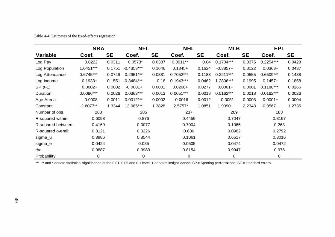
49
Table 4-4: Estimates of the fixed-effects regression
Variable Coef. SE Coef. SE Coef. SE Coef. SE Coef. SE
Log Pay 0.0222 0.0311 0.0573* 0.0337 0.0911** 0.04 0.1704*** 0.0375 0.2254*** 0.0428
Log Population 1.0451*** 0.1751 -0.4353*** 0.1646 0.1345+ 0.1624 -0.3857+ 0.3122 0.0363+ 0.0437
Log Attendance 0.6745*** 0.0749 0.2951*** 0.0881 0.7052*** 0.1188 0.2211*** 0.0555 0.6509*** 0.1438
Log Income 0.1933+ 0.1551 -0.8484*** 0.16 0.1943*** 0.0462 1.2806*** 0.1995 0.1457+ 0.1858
SP (t-1) 0.0002+ 0.0002 -0.0001+ 0.0001 0.0268+ 0.0277 0.0001+ 0.0001 0.1188*** 0.0266
Duration 0.0086*** 0.0026 0.0363*** 0.0013 0.0051*** 0.0018 0.0162*** 0.0018 0.0162*** 0.0026
Age Arena -0.0008 0.0011 -0.0012*** 0.0002 -0.0016 0.0012 -0.005* 0.0003 -0.0001+ 0.0004
Constant -2.6077** 1.3344 12.085*** 1.3828 2.5757* 1.0851 1.9090+ 2.2343 -0.9567+ 1.2735
Number of obs.
R-squared within:
R-squared between:
R-squared overall:
sigma_u
sigma_e
rho
Probability
***, ** and * denote statistical signif icance at the 0.01, 0.05 and 0.1 level, + denotes insignif icance; SP = Sporting performance; SE = standard errors.
263 285 237 269 183
NBA NFL NHL MLB EPL
0.4169 0.0077 0.7004 0.1065 0.263
0.6098 0.876 0.4459 0.7047 0.8197
0.3986 0.8544 0.1061 0.6517 0.3016
0.3121 0.0226 0.636 0.0982 0.2792
0.9887 0.9983 0.8154 0.9947 0.976
0.0424 0.035 0.0505 0.0474 0.0472
0 0 0 0 0

Chapter 4: Sport or Business Approach? A Cross-Continent Analysis of U.S. Major
League Franchises and English Premier League Clubs
50
In summary, the differences in the determinants that influence team values and
revenues between North American major leagues and the English Premier League is
apparent only through a close consideration of sporting performance. To explicate the
results from the regression analysis in more detail, the next section focuses on athletic
and financial efficiency results as well.
4.6.2 DEA Efficiency Results
On the basis of an efficiency analysis with an assumption of constant returns to
scale, Table 4-5 provides the bootstrapped global technical efficiency scores for
sporting technical efficiency, for which winning percentage or relative points obtained
in season t is the output. Table 4-6 then presents the global technical efficiency scores
for financial efficiency, where franchise values or revenues for EPL are the output. The
input factors are identical to the explanatory variables applied in the regression analysis.
The separate analyses for each league reflect each team’s annual efficiency scores for
2001-2009, using a comparison of each team with its peers on an annual basis.
Table 4-5: Global technical efficiency scores for sporting efficiency
2001 2002 2003 2004 2005 2006 2007 2008 2009 Mean
EPL 0.905 0.928 0.950 0.879 0.806 0.915 0.892 0.919 0.972 0.907
NBA 0.840 0.828 0.805 0.767 0.813 0.856 0.824 0.744 0.791 0.807
NFL 0.718 0.809 0.735 0.739 0.703 0.763 0.685 0.710 0.697 0.729
NHL 0.886 0.914 0.887 0.922 - 0.855 0.875 0.941 0.940 0.902
MLB 0.934 0.928 0.911 0.933 0.926 0.939 0.905 0.869 0.942 0.921
In the test to determine if the overall sporting efficiency in the EPL exceeds that
of the major league franchises—which would affirm that the EPL is more win-oriented

Chapter 4: Sport or Business Approach? A Cross-Continent Analysis of U.S. Major
League Franchises and English Premier League Clubs
51
than its North American counterparts—the EPL actually ranked second, with a mean
efficiency of 0.907, whereas the mean efficiency of MLB was 0.921. In general, these
results indicated that the two leagues achieved 90.7% and 92.1% of their potential,
respectively. The mean efficiency scores across the other major league franchises varied
considerably, such that NFL franchises exhibited an efficiency score of just 0.729, and
the NBA franchises reached 0.807. Applying a t-test proves that the difference of means
between the leagues is statistically significant different from 0.15
The likely explanation
for the considerably lower score for the NFL again derives from the revenue-sharing
regulations. Regardless of their level of success on the field, NFL franchises receive a
fixed percentage of the league’s overall revenues, such as those earned through
broadcasting contracts. Therefore, NFL franchises do not depend as much on local
income, such as game-day revenues, as the other major leagues do.
This argument also received support from the results for financial efficiency in
Table 6, because the revenue-maximising major league franchises performed closer to
the efficiency frontier than the win-maximising EPL clubs. That is, all the North
American major leagues reported higher overall mean efficiency scores than those
obtained by the EPL. The NBA and NFL franchises were the top ranked, with overall
mean efficiency values of 0.919 and 0.909, respectively, followed by MLB (0.897) and
NHL (0.886) franchises. The EPL’s overall mean efficiency score of 0.878 ranked last.
In a comparison with the results for sporting efficiency, if the NBA and NFL are
excluded as outliers, all leagues operated in similar proximity to the economic frontier,
15
The p-Value of 0.000 denotes rejecting the null hypothesis that the difference between the means is
zero.

Chapter 4: Sport or Business Approach? A Cross-Continent Analysis of U.S. Major
League Franchises and English Premier League Clubs
52
such that the difference between the first ranked NBA and last ranked EPL was
relatively small.
Table 4-6: Global technical efficiency scores for financial efficiency
2001 2002 2003 2004 2005 2006 2007 2008 2009 Mean
EPL 0.882 0.848 0.841 0.919 0.901 0.828 0.909 0.885 0.890 0.878
NBA 0.937 0.946 0.905 0.926 0.875 0.911 0.911 0.922 0.938 0.919
NFL 0.812 0.869 0.929 0.934 0.915 0.925 0.955 0.922 0.922 0.909
NHL 0.901 0.867 0.877 0.902 - 0.898 0.886 0.871 0.882 0.886
MLB 0.884 0.882 0.882 0.891 0.899 0.899 0.922 0.932 0.878 0.897
Finally, the analysis of the margin of efficiency scores, as summarised in Table 4-
7, confirmed the hypothesis that the major league franchises tend to be business driven.
Margin of efficiency scores reflect the difference between sporting and financial
technical efficiency. In this analysis, a greater positive value indicated the
predominance of a sporting focus, whereas an increasing negative value suggested a
business-oriented organization. If the margin between sporting and financial efficiency
was smaller, the two factors appeared more balanced.
Table 4-7: Global technical efficiency margin scores of sporting and financial efficiency
2001 2002 2003 2004 2005 2006 2007 2008 2009 Mean
EPL 0.023 0.079 0.109 -0.040 -0.095 0.087 -0.017 0.034 0.082 0.029
NBA -0.097 -0.118 -0.099 -0.159 -0.063 -0.055 -0.087 -0.178 -0.147 -0.112
NFL -0.095 -0.059 -0.194 -0.195 -0.212 -0.162 -0.269 -0.213 -0.226 -0.181
NHL -0.015 0.047 0.009 0.020 - -0.043 -0.010 0.069 0.058 0.017
MLB 0.051 0.046 0.029 0.042 0.026 0.040 -0.017 -0.064 0.064 0.024

Chapter 4: Sport or Business Approach? A Cross-Continent Analysis of U.S. Major
League Franchises and English Premier League Clubs
53
In this comparison, the EPL emerged with the highest positive value across all
leagues, in support of the sporting rationale. The calculations for MLB and NHL also
show positive values; the NFL and NBA revealed negative values. Thus, the results
aligned with the prediction that North American major league franchises would be more
focused on business, while EPL clubs pursue success on the field.
4.7 Summary and Concluding Remarks
In investigating the determinants of major league and English Premier League
franchise values and revenues, this study shows that the impact of athletic achievement
on financial performance is significant only for EPL clubs, not for teams in North
American major leagues. The analyses of the different leagues’ sporting and financial
efficiency support the sporting hypothesis, which holds that EPL clubs value sporting
performance over financial performance, in contrast with the major league franchises.
This outcome might also reflect the differences in the league systems; for example, in
European soccer leagues, an improved league position directly increases revenues, by
granting those teams the right to participate in European competitions. In the major
leagues, revenue sharing and drafting rights instead ensure consistent revenues and
benefits, even for franchises with an inferior sporting performance.
Due to data constraints the applied sample is composed by four U.S. leagues and
solely one European league and might be unbalanced in geographic representativity. In
addition, all leagues belong to different sports and consequently the observed
differences might not be explained only by a difference in pursued objectives.
Accordingly, further studies should investigate whether other European leagues
(e.g., Spanish Primera Division, German Bundesliga) exhibit similar efficiency levels in

Chapter 4: Sport or Business Approach? A Cross-Continent Analysis of U.S. Major
League Franchises and English Premier League Clubs
54
their sporting and financial performance. Additional research also could draw
comparisons with other leagues, to examine the extent to which sporting performance
influences team values and revenues. However, such investigations could be hindered
by the lack of publicly available data.
Chapter 5: Does Performance Consistency Pay-Off Financially for Players? Evidence
from the Bundesliga
55
5 Does Performance Consistency Pay-Off Financially for Players?
Evidence from the Bundesliga
5.1 Introduction
In recent years professional team sports steadily gained popularity around the
globe entailing an expanding industry with large revenues and increasing employment.
Coincidental professional team sports drew the attention of academics as numerous
economic studies have been published in the field of sports economics ever since. A
particularly popular strand of literature analyses the remuneration of professional
athletes to explain observable wage dispersions in professional sports. Previous studies
in the field frequently relied on the Mincerian income equation (1974) to analyze the
impact of manifold drivers of salary. Several individual characteristics including age,
experience, talent, position, team effects, country of origin and especially average
performance have been found to define player salaries. By contrast, research concerning
consistency of performance is still in the beginning. This is to some extent surprising as
supposedly owners and managers would favor high consistency in performance by their
employees in order to reduce monitoring costs as well as the uncertainty of output
generation. Maybe surprisingly our estimations reveal that while average performance
influences salary in a significant positive way, consistency of performance reduces
players’ remuneration.
The current research is innovative by closing this gap in the literature and
providing a novel approach as we analyze game level data from the German Bundesliga
soccer for five consecutive seasons between 2005-06 and 2009-10. The data set contains
information for 845 different players and totals in 34,413 game-level performance
Chapter 5: Does Performance Consistency Pay-Off Financially for Players? Evidence
from the Bundesliga
56
observations. To measure performance consistency, the variation coefficient over each
season is calculated for player evaluations compiled by experts and published in
“Kicker Sportmagazin”, a highly respected soccer magazine. To the best of our
knowledge, this is the first empirical approach to determine if consistency in player
performance is rewarded monetarily in professional soccer. Further, our research
disentangles the influence of consistency for different parts of the salary distribution
providing information if consistency of performance by “star-players” have a different
impact on salary compared to average players. Our analysis suggests that the negative
impact of consistency on salary is observable for different parts of the salary
distribution. Finally, we present suggestions for these unreckoned findings to identify
avenues for further research in this understudied field highlighting the importance of
sport specific impact by its given rules and regulations.
The chapter is organized as follows: The next section provides a review of the
existing literature on salary determination in professional soccer followed by a brief
discussion of the results. Section 3 introduces the applied data, specifies our model and
presents the results of the empirical analysis. The paper concludes with a discussion of
the empirical results and limitations to present an outlook on future research.
5.2 Literature Review
Fertilized by available and detailed information on player salaries, performance
statistics and individual characteristics a large number of studies have already been
published on the drivers of remuneration in professional soccer. When it comes to
performance related information studies uniformly rely on average performance (mostly
from the previous season) neglecting if players perform consistently or volatile.
Chapter 5: Does Performance Consistency Pay-Off Financially for Players? Evidence
from the Bundesliga
57
Concerning professional soccer Bryson, Frick & Simmons (2013) find empirical
evidence of a salary premium for two-footedness as well as a statistically significant
impact of players’ age, number of international appearances and position on the pitch.
Similar results for age and experience are repeatedly reported in the literature
(Lehmann, 2000; Huebl & Swieter, 2002; Lucifora & Simmons, 2003; Garcia-del-
Barrio & Puyol, 2007; Wicker et al., 2013). Continuously determined is a reversed U-
shaped relationship between age and salary as physical performance erodes over time.
In addition, salaries reportedly rise with experience, as in number of league games
(Lehmann & Weigand, 1999; Huebl & Swieter, 2002; Frick, 2007) as well as
international appearances for the national team or appearances in European and World
Cups (Lucifora & Simmons, 2003; Franck & Nüesch, 2008; Lehmann & Schulze, 2008)
entail higher salaries, again supporting diminishing returns.
Previous research also accounts for the position on the field and its impact on
salary. Studies predominantly report that more offensive positions are paid a wage
premium (Huebl & Swieter, 2002; Lucifora & Simmons, 2003; Frick, 2006). Due to
their high specialization and low flexibility to take other positions on the field
goalkeepers on average earn the least while forwards receive the highest salaries
(Lehmann, 2000).
Studies focusing on the major North American sport leagues (NBA, NFL, MLB,
NHL and MLS) also found a significant impact of experience, performance and peer
reputation on players´ salary (Kahn, 1993; Hamilton, 1997; Quirk & Fort, 1999; Idson
& Kahane, 2000; Zimbalist, 2002; Berri & Simmons, 2009; Lee & Harris, 2012).
Perhaps surprisingly, to the best of our knowledge only one empirical work is

Chapter 5: Does Performance Consistency Pay-Off Financially for Players? Evidence
from the Bundesliga
58
concerned with players’ consistency to explain salary. Bodvarsson & Brastow (1998)
analyze players from the National Basketball Association. They follow the argument
that for a given average performance coaches as well as general managers prefer
consistent over volatile performance. Compared to their study our work offers several
important contributions. First, in contrast to Bodvarsson & Brastow (1998) our data
offers information over several seasons, allowing for a longitudinal analysis controlling
for unobservable factors. Given the large number of observations we are furthermore
able to control for team, season and position effects. In addition, we extend
understanding of how consistency of performance is rewarded or punished for different
parts of the salary distribution by applying quantile regressions. Further, we are able to
rely on a single performance measure accounting for overall performance which is
unavailable in other sports. An overview of previous literature and the empirical
findings is provided in Table 5-1.
Summarizing, it appears that salaries in professional soccer are not just random,
but that systematic factors determine salaries to a large extent and that these systematic
factors (e.g. age, experience and performance) are very similar to those found for other
occupations (Bryson, Frick & Simmons, 2013). However, the variation in salaries in
professional sports that can be explained by a small set of variables is quite large
compared to studies analyzing representative labor market surveys. What previous
studies have in common is a recurrent measurement of average performance to
determine its impact on salary (see Table 5-1). As not all participants in sports are
identical in terms of performance consistency, our research expands existing work as we
account for volatility in performance. The relation to labor markets is straightforward.
While some individuals are able to perform at a very consistent rate others do not. The

Chapter 5: Does Performance Consistency Pay-Off Financially for Players? Evidence
from the Bundesliga
59
question arises how managers value consistency by determining the financial surplus to
the athlete. One argument in favor of a salary premium for consistent performance
follows the rationale of monitoring costs. Monitoring costs are presumably lower for
workers displaying a constant productivity compared to those whose performance is
rather volatile. For a given average performance monitoring costs decrease as
consistency increases which leads to the assumption that salary offers are higher for
those employees who are performing more consistently.16
For professional soccer the
implication might not be that straightforward, since the composition of workforces
differs dramatically from those of companies competing in traditional markets. Firstly,
performance can be observed easily and hence at lower costs. This would suggest less
difference in salaries due to variance in performance. Secondly, coaches can simply
substitute players displaying a bad performance in the production process. This might
even result in a preference towards inconsistent players as performance outliers reach
higher levels for inconsistent players who can be substituted or simply disregarded in
the initial line-up. A possible result of this could be a wage premium for inconsistent
players.
Given these arguments the relation between performance consistency and salary
remains unclear from a theoretical standpoint. As game-by-game performance is
observable for soccer we are able to estimate how consistency affects remuneration for
the specific labor market the German Bundesliga.
16
See Bodvarsson & Brastow (1998).

60
Table 5-1: Literature on salary determination for professional soccer
Author(s) Data Applied Model Empirical Findings
Wicker et al. (2013) Sample of 877 players from the
2011-12 and 2012-13 season of
the German Bundesliga
Fixed- and random effects
regression with natural
logarithm of market value
The results indicate that effort
approximated by running distance and
average number of intensive runs has
no significant positive impact Games
played, age as well as scoring
performance show a positive impact on
market values
Bryson, Frick & Simmons (2013) Data 1: 1,991 European league
players of the 2005-06 season
Data 2: Bundesliga panel with
1,314 player-season observations
over 2002-03 to 2006-07
OLS and quantile regressions
with natural logarithm of
annual salary
The authors find empirical evidence
that the ability of two-footedness is
rewarded monetarily. Further, variables
such as age, height, goals per game in
the last season as well as international
appearances generate an increment in
salary
Frank & Nüesch (2008) Sample of 429 players from
2004-05 German Bundesliga
season
OLS and quantile regression
with natural logarithm of
market value
Empirical findings indicate that market
values are better predicted by expert
evaluations. Goals and assists have no
significant impact whereas player´s
popularity influence market values
Garcia-del-Barrio & Puyol (2007) Sample of 369 players appearing
in the Spanish Primera Division
in 2001-02
OLS regression with natural
logarithm of market value The results display that commercial
attractiveness (measured by Google
hits), sporting performance (measured
by external ratings) and international
experience of players are rewarded
monetarily

61
Table 5-1: Literature on salary determination for professional soccer (continued)
Author(s) Data Applied Model Empirical Findings
Lucifora & Simmons (2003) 1995-96 single season data
including 730 outfield players
from the Italian Serie A & B
OLS regression with natural
logarithm of gross salary The results reveal the presence of a
superstar effect on salary as well as
significant impacts of experience,
performance and reputation on salary
Huebl & Swieter (2002) Panel data set for the seasons
1994-95 to 1999-2000 containing
574 player appearances in the
German Bundesliga
OLS and random-effects with
natural logarithm of annual
salary
The authors find a reversed U-shaped
relationship between age, career games
and salary. In addition, the authors find
an impact of contract duration, team
change, sponsoring revenues as well as
qualification for European cups on
salary
Lehmann (2000) 1999-2000 single season data
including 463 player
observations from German
Bundesliga
OLS regression with natural
logarithm of annual salary Positive influence of games played last
season, country of origin, tackles,
assists and sponsoring revenues on
salary. In contrast, substitutions are
reported to have a negative impact
Lehmann & Weigand (1999) 1998-99 single season data
including 468 player
observations from German
Bundesliga
OLS regression with natural
logarithm of annual salary The authors find evidence that career
games, country of origin, attendance,
sponsoring revenues and qualification
for European cups impact salaries
Chapter 5: Does Performance Consistency Pay-Off Financially for Players? Evidence
from the Bundesliga
62
5.3 Data Set and Descriptive Statistics
The data set we analyze in this paper contains season statistics for all players who
appeared in the German Bundesliga anytime between the 2005-06 and the 2009-10
season. In addition to average statistics we gathered game-by-game performance
measures for each game a player appeared in and had been rated by external experts.
Our data set contains 845 different players and yields in 34,413 player-match day-
observations. The Bundesliga continuously consisted of 18 teams with 34 match days in
each of the five analyzed seasons and therefore the data set includes player statistics
from a total of 3,060 season games. In contrast to the closed-shop major leagues in the
U.S. most European leagues apply a relegation and promotion system. Each season the
three worst performing teams in the German Bundesliga are replaced by the top three
teams from the second division (2nd Bundesliga) resulting in a varying composition of
the league over the analyzed period. During the five seasons 26 different clubs played in
the Bundesliga due to annual promotion and relegation.
The primary data source for this study is the highly respected German sports
journal “Kicker Sportmagazin” that publishes salary estimations prior to the start of
each season as a reliable proxy for the otherwise undisclosed salary. Based on previous
publications we approximate salaries for season t as follows:
𝑆𝑎𝑙𝑎𝑟𝑦 (𝑡) = 𝑘𝑖𝑐𝑘𝑒𝑟 𝑣𝑎𝑙𝑢𝑎𝑡𝑖𝑜𝑛 (𝑡)
1.5

Chapter 5: Does Performance Consistency Pay-Off Financially for Players? Evidence
from the Bundesliga
63
The reliability of this salary information has been documented repeatedly:
Torgler and Schmidt (2007) confirmed robustness by comparing salary information by
Kicker with the market value evaluations by www.transfermarkt.de, another reliable
data source. The correlation between the two data sources is reported to be as high as
0.75. Furthermore, Frick (2006) correlates the salary information by Kicker with a
subset of actual salary data for 2 seasons from the Bundesliga finding the correlation to
be high as 0.8. Further studies using the salary estimations by “Kicker” include
Eschweiler & Vieth (2004), Hübl & Swieter (2002), Lehmann & Weigand (1999), as
well as Lehmann & Schulze (2005). Our study follows this literature and uses this proxy
to analyze the impact of performance consistency on player salaries.
Moreover, Kicker weekly publishes a subjective individual performance
evaluation following each Bundesliga match. It accounts for overall performance
throughout the match as the output of professional players is highly complex and can
hardly be defined by only one objective measure such as number of tackles, goals
scored or assists. This is especially useful because of the varying job descriptions
(goalkeeper, defender, midfielder, forward) as each position is assigned with a different
duty (see Lehmann & Weigand, 1999; Lucifora & Simmons, 2003; Frank & Nüesch,
2010). Trusting evaluations by experts is common practice in the sport economics
literature (Littkemann & Kleist, 2002; Garcia-del-Barrio & Pujol, 2005; Bryson, Frick
& Simmons, 2013). Performance evaluation is comparable to performance measuring in
the German school system and itemizes grades from 1.0 (excellent) to 6.0 (very poor).
To receive grading after a match a player has to be on the pitch for a minimum of 30
minutes.
Chapter 5: Does Performance Consistency Pay-Off Financially for Players? Evidence
from the Bundesliga
64
Our analyses accounts for the average grade (GRD) over a season as we set the
minimum number of appearances during a season to five.
The main contribution of this paper is to shed light on the impact of consistency
of performance on salaries of professional soccer players in Germany. We define
consistency as the deviation of performance around average performance for a given
player and season. Consequently we analyze to what extent variations in player
performance explain variations in player remuneration. As variance increases with the
mean we compute the variation coefficient (VAR) of performance over a season as
follows:
𝑉𝑎𝑟𝑖𝑎𝑡𝑖𝑜𝑛 𝑐𝑜𝑒𝑓𝑓𝑖𝑐𝑖𝑒𝑛𝑡 (𝑡) = 𝑉𝑎𝑟𝑖𝑎𝑛𝑐𝑒 (𝑡)
∅ 𝐺𝑟𝑎𝑑𝑒 (𝑡)
Admittedly one could argue that for a given variance in performance, a higher
(worse) average grade reduces the coefficient of variation. To lessen this concern, all
results to follow still hold as we conduct the estimations substituting the variation
coefficient of performance by the variance of performance to display performance
consistency.
Apart from (average) performance and its consistency other factors possibly
determining players’ salaries have to be accounted for. Previous job experience is
expected to have a positive impact on remuneration according to human capital theory.
Our measures for age (AGE), games played in the Bundesliga (BLG) and number of
appearances on national squads (NAT) (all measured prior to the respective season)
display players’ experience. We expect a positive impact of experience on salary

Chapter 5: Does Performance Consistency Pay-Off Financially for Players? Evidence
from the Bundesliga
65
accompanied with decreasing marginal returns (negative impact of AGE2, BLG2 and
NAT2), equivalent to an upward-sloping experience-earnings profile. To account for
any positional or team bias in ratings we include team as well as season dummies. Team
effects are supposed to have a significant influence on player salaries as some teams
were found to pay their players a premium salary (Idson & Kahane, 2000; Frick, 2008).
A summary of all variables included is presented in Table 5-2 while summary statistics
are provided in Table 5-3.
Table 5-2: Overview of variables
Variable Operationalization
lnPAY natural logarithm salary
VAR (t-1) Variation coefficient of performance evaluation (T-1)
GRD (t-1) performance evaluation (T-1)
AGE Age (at beginning of season)
AGE2 squared age (at beginning of season)
NAT (career) appearances national team (at beginning of season)
NAT2 (career) squared appearances national team (at beginning of season)
BLG (career) Bundesliga career games (at beginning of season)
BLG2 (career) squared Bundesliga career games (at beginning of season)
GK Goalkeeper (Dummy; 1=yes) Reference
DEF Defender (Dummy; 1=yes)
MID Midfielder (Dummy; 1=yes)
FOR Forward (Dummy; 1=yes)
Team Dummies Dummy-variable for players´ team
Season Dummies Dummy-variable for analyzed season
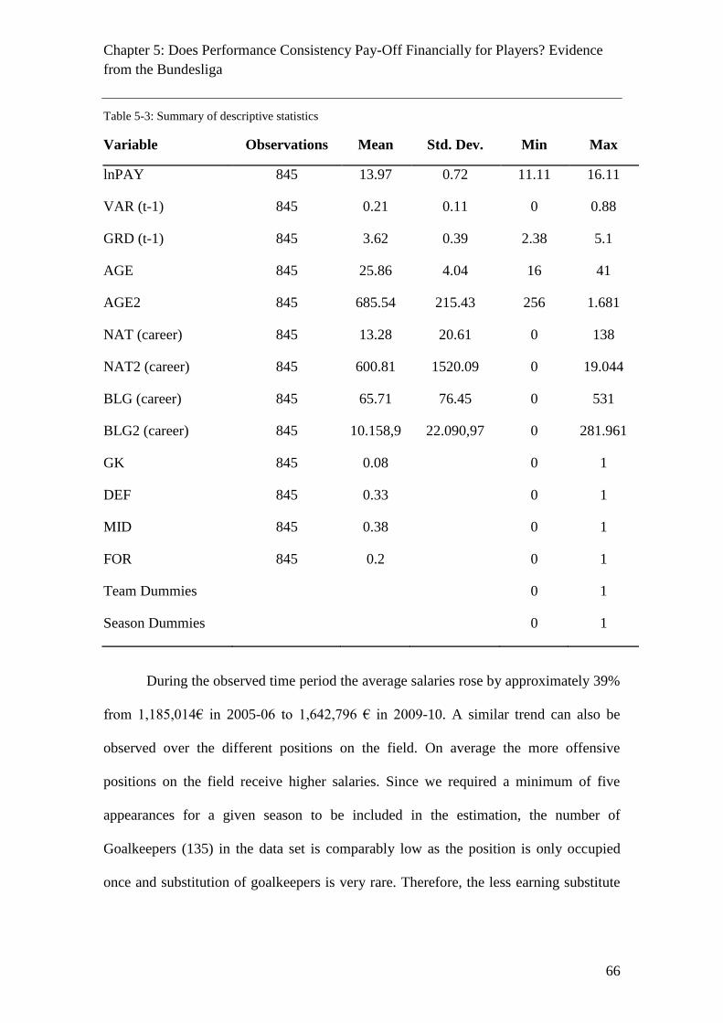
Chapter 5: Does Performance Consistency Pay-Off Financially for Players? Evidence
from the Bundesliga
66
Table 5-3: Summary of descriptive statistics
Variable Observations Mean Std. Dev. Min Max
lnPAY 845 13.97 0.72 11.11 16.11
VAR (t-1) 845 0.21 0.11 0 0.88
GRD (t-1) 845 3.62 0.39 2.38 5.1
AGE 845 25.86 4.04 16 41
AGE2 845 685.54 215.43 256 1.681
NAT (career) 845 13.28 20.61 0 138
NAT2 (career) 845 600.81 1520.09 0 19.044
BLG (career) 845 65.71 76.45 0 531
BLG2 (career) 845 10.158,9 22.090,97 0 281.961
GK 845 0.08 0 1
DEF 845 0.33 0 1
MID 845 0.38 0 1
FOR 845 0.2 0 1
Team Dummies 0 1
Season Dummies 0 1
During the observed time period the average salaries rose by approximately 39%
from 1,185,014€ in 2005-06 to 1,642,796 € in 2009-10. A similar trend can also be
observed over the different positions on the field. On average the more offensive
positions on the field receive higher salaries. Since we required a minimum of five
appearances for a given season to be included in the estimation, the number of
Goalkeepers (135) in the data set is comparably low as the position is only occupied
once and substitution of goalkeepers is very rare. Therefore, the less earning substitute

Chapter 5: Does Performance Consistency Pay-Off Financially for Players? Evidence
from the Bundesliga
67
goalkeepers are seldom included in the sample. Waiving our minimum number of
appearances the average salary of goalkeepers would drop below the average salary of
defenders.
Concerning average performance Figure 5-1 suggests that goalkeepers receive
the lowest (best) whereas forwards receive the highest (worst) ratings. Defenders and
midfielders receive almost identical average ratings. Interestingly, out of all players who
were graded with 1.0 (excellent) for a single game forwards accounted for 55%. In
contrast, goalkeepers only accounted for 15% of the top grades but also account for 9%
of all player appearances.
Figure 5-1: Average expert ratings by position
The variation coefficient for performance by position is documented in Figure 5-
2. Comparable to the variable average performance, our key variable displaying
consistency, influences players’ salaries also shows positional differences. In particular
for the offensive forwards and midfielders we observe a higher variation coefficient
0
2,5
5
2005 2006 2007 2008 2009
Goal Defender Midfield Forward
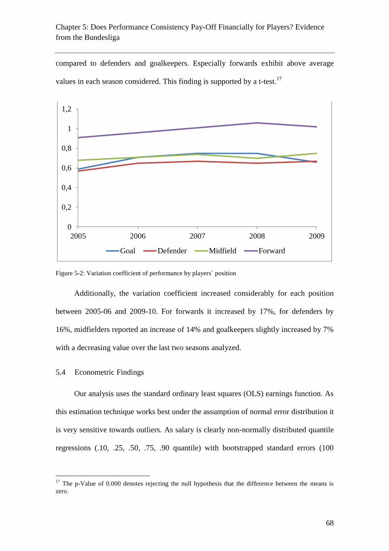
Chapter 5: Does Performance Consistency Pay-Off Financially for Players? Evidence
from the Bundesliga
68
compared to defenders and goalkeepers. Especially forwards exhibit above average
values in each season considered. This finding is supported by a t-test.17
Figure 5-2: Variation coefficient of performance by players´ position
Additionally, the variation coefficient increased considerably for each position
between 2005-06 and 2009-10. For forwards it increased by 17%, for defenders by
16%, midfielders reported an increase of 14% and goalkeepers slightly increased by 7%
with a decreasing value over the last two seasons analyzed.
5.4 Econometric Findings
Our analysis uses the standard ordinary least squares (OLS) earnings function. As
this estimation technique works best under the assumption of normal error distribution it
is very sensitive towards outliers. As salary is clearly non-normally distributed quantile
regressions (.10, .25, .50, .75, .90 quantile) with bootstrapped standard errors (100
17
The p-Value of 0.000 denotes rejecting the null hypothesis that the difference between the means is
zero.
0
0,2
0,4
0,6
0,8
1
1,2
2005 2006 2007 2008 2009
Goal Defender Midfield Forward

Chapter 5: Does Performance Consistency Pay-Off Financially for Players? Evidence
from the Bundesliga
69
repetitions) are applied to estimate varying marginal effects of the independent variables
at different parts of the salary distribution.
A possible endogeneity problem between performance and salary was met by the
introduction of a time lag of one season. While salary information is obtained from
season t, the independent variables concerning performance are drawn from the
respective previous season t-1.
The empirical specification adopted is
𝑙𝑛𝑃𝐴𝑌𝑡 = 𝑎0 + 𝑎1 𝑉𝐴𝑅𝑡−1 + 𝑎2 𝐺𝑅𝐷𝑡−1 + 𝑎3 𝐴𝐺𝐸𝑡 + 𝑎4 𝐴𝐺𝐸²𝑡 + 𝑎5 𝑁𝐴𝑇𝑡−1
+ 𝑎6 𝑁𝐴𝑇²𝑡−1 + 𝑎7 𝐵𝐿𝐺𝑡 + 𝑎8 𝐵𝐿𝐺²𝑡 + 𝑎9 𝐺𝑆𝐶𝑡 + 𝑎10 𝑃𝑂𝑆𝐼𝑇𝐼𝑂𝑁𝑡−1
+ 𝑎11 𝑇𝐸𝐴𝑀𝑡 + 𝑎12 𝑆𝐸𝐴𝑆𝑂𝑁𝑡 + 𝜀
Where lnPAYt represents the natural log of the salary, 𝑎0is a constant, 𝑎1 to 𝑎12 are
vectors of parameters to be estimated and ɛ is an error term. Given the panel structure of
the data the Hausman test suggests to rely on the fixed-effects estimation implying that
unobserved player characteristics are present.18
18
Results from Hausman test (Hausman, 1978):
= 98.61, p < .05.

Chapter 5: Does Performance Consistency Pay-Off Financially for Players? Evidence
from the Bundesliga
70
Estimation for OLS- and fixed-effects regressions are presented in Table 5-4.
Table 5-4: Estimation results for OLS and fixed-effects regressions
lnPay OLS robust Fixed-Effects
VAR (t-1) 0.9231***
0.4269***
GRD (t-1) -0.7216***
-0.4863***
AGE 0.0881**
-0.2276+
AGE2 -0.0022***
-0.0038*
NAT (career) 0.0055***
-0.0018+
NAT2 (career) -0.0001+
-0.0001+
BLG (career) 0.0017***
0.0133***
BLG2 (career) -0.0009**
-0.0001***
DEF 0.1585**
0.0024+
MID 0.1975***
0.0529+
FOR 0.3652***
0.2168**
CONS 15.66***
18.36***
Team Dummies included
Season Dummies included
N of Obs. 845 845
N of Players 432 --
R2*100 58.01 42.12
F-Value 31.90*** 8.64***
sigma_u -- 0.7471
sigma_e -- 0.2408
rho -- 0.9058
***, ** and * denote statistical significance at the 0.01, 0.05 and 0.1 level, + denotes insignificance.
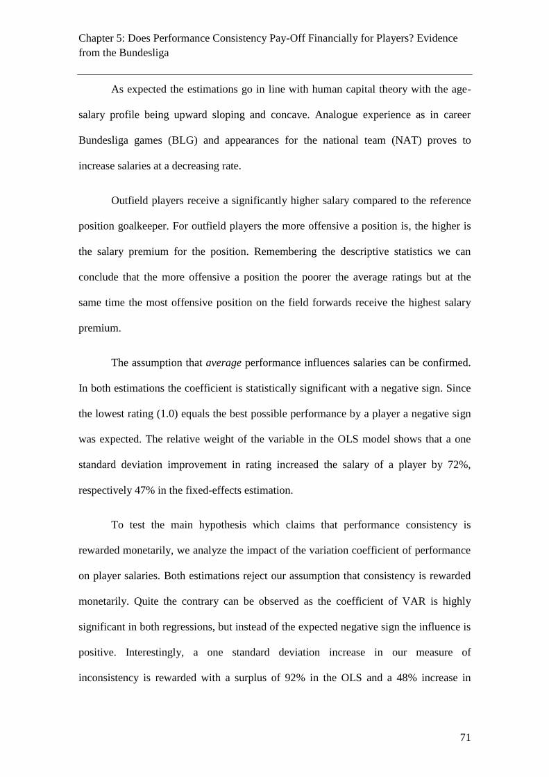
Chapter 5: Does Performance Consistency Pay-Off Financially for Players? Evidence
from the Bundesliga
71
As expected the estimations go in line with human capital theory with the age-
salary profile being upward sloping and concave. Analogue experience as in career
Bundesliga games (BLG) and appearances for the national team (NAT) proves to
increase salaries at a decreasing rate.
Outfield players receive a significantly higher salary compared to the reference
position goalkeeper. For outfield players the more offensive a position is, the higher is
the salary premium for the position. Remembering the descriptive statistics we can
conclude that the more offensive a position the poorer the average ratings but at the
same time the most offensive position on the field forwards receive the highest salary
premium.
The assumption that average performance influences salaries can be confirmed.
In both estimations the coefficient is statistically significant with a negative sign. Since
the lowest rating (1.0) equals the best possible performance by a player a negative sign
was expected. The relative weight of the variable in the OLS model shows that a one
standard deviation improvement in rating increased the salary of a player by 72%,
respectively 47% in the fixed-effects estimation.
To test the main hypothesis which claims that performance consistency is
rewarded monetarily, we analyze the impact of the variation coefficient of performance
on player salaries. Both estimations reject our assumption that consistency is rewarded
monetarily. Quite the contrary can be observed as the coefficient of VAR is highly
significant in both regressions, but instead of the expected negative sign the influence is
positive. Interestingly, a one standard deviation increase in our measure of
inconsistency is rewarded with a surplus of 92% in the OLS and a 48% increase in

Chapter 5: Does Performance Consistency Pay-Off Financially for Players? Evidence
from the Bundesliga
72
player salaries in the fixed-effects model. For a given average performance managers
and team owners seem to prefer unpredictable players that on a good day might make
the difference in order to win a match.
In the 2009-10 season the 25% highest paid players accounted for 46% of the
total sum of salaries paid. This skewed income distribution can be explained with
Rosen´s theory of superstars where small differences in talent translate into large
differences in pay (Rosen, 1981, 1983), supported by Figure 3. Applying the
D´Agostino test (D´Agostino, Belanger & D´Agostino Jr., 1990) we get further approve
that salaries significantly differ from a normal distribution.19
Figure 5-3: Kernel Density Estimates of player salaries
19
The p-value of 0.000 suggests rejecting of the null hypothesis that kurtosis does not depart from a
normal distribution.
0.2
.4.6
Den
sity
11 12 13 14 15 16lnpay
Kernel density estimate
Normal density

Chapter 5: Does Performance Consistency Pay-Off Financially for Players? Evidence
from the Bundesliga
73
Given this skewed distribution previous studies called for quantile regressions,
originally developed by Koenker and Bassett (1978), (see Hamilton, 1997; Franck &
Nüesch, 2008; Lehmann & Schulze, 2008; Berri & Simmons, 2009; Simmons & Berri,
2009; Vincent & Eastman, 2009; Kahane, 2010 for sports economics applications). The
particular advantage of quantile regression is to measure the impact of performance and
characteristics for different parts of the salary distribution (Koenker, 2005). In order to
ensure robustness of standard errors, we apply bootstrapping with 100 replications. The
results of the quantile regressions are reported in Table 5-5.
Table 5-5: Impact of consistent performance on salary (Quantile Regressions)
lnPay 0.1 0.25 0.5 0.75 0.9
VAR (t-1) 1.1094** 1.2123*** 1.0068*** 0.9535*** 1.0349***
GRD (t-1) -0.7522*** -0.7691*** -0.7579*** -0.7041*** -0.6292***
AGE 0.1476** 0.1531** 0.1191** -0.0001+ 0.0465+
AGE2 -0.0034** -0.0035** -0.0028** -0.0003+ -0.0011+
NAT (career) 0.0052* 0.0061** 0.0054** 0.0038+ 0.0042**
NAT2 (career) -0.0001+ -0.0001* -0.0197+ -0.0081+ -0.0001+
BLG (career) 0.0041*** 0.0028** 0.0021*** 0.0016** 0.0012**
BLG2 (career) -0.0001*** -0.0141+ -0.0118** -0.0091** -0.0098***
DEF 0.2710** 0.2711** 0.2163** 0.1258+ 0.0735+
MID 0.2203** 0.3091** 0.2881*** 0.1699** 0.1527**
FOR 0.4342*** 0.4348*** 0.4348*** 0.3175*** 0.2211***
CONS 14.69*** 14.76*** 17.64*** 16.84*** 17.99***
Team Dummies included
Season Dummies included
N of Obs. 845
Pseudo R2*100 31.64 34.62 39.29 42.12 44.45
***, ** and * denote statistical significance at the 0.01, 0.05 and 0.1 level, + denotes insignificance.

Chapter 5: Does Performance Consistency Pay-Off Financially for Players? Evidence
from the Bundesliga
74
The estimations retrieved from the quantile regression in general support the
results obtained from the OLS and fixed-effects regression revealing further interesting
insights. The results demonstrate that AGE only seems to influence salary for the lower
paid players at the .10, .25 and .50 quantile whereas BLG remains significant for all
quantiles with a constant decreasing influence as salaries increase. Also international
experience (NAT) remains significant for all quantiles with a decreasing impact as
salaries rise. The position a player contains also loses importance as the bonus for the
offensive positions MID and FOR diminishes.
Paying attention to the main variables we observe that both performance
measures are statistically significant throughout all quantiles. In addition, the average
performance displays a surplus of up to 76% for the .25 and .50 quantile.
Regarding performance consistency the quantile regressions even strengthen the
results from the OLS and fixed-effects regression. Therefore, inconsistency or the
characteristic of a player to be unpredictable is rewarded monetarily. The salary
premium is reported for all quantiles in the sample.
5.5 Summary and Concluding Remarks
Since little is known about the impact of consistency on player remuneration in
professional sports this paper presents insights for professional soccer in Germany. We
find strong evidence for a salary premium for players who perform inconsistently.
These results contradict the findings by Bodvarsson & Brastow (1998) who were the
first to empirically analyze the relationship between pay and consistency in
performance. Instead of rewarding consistency general managers seem to reward
inconsistency in performance monetarily. A possible explanation for the contrary results
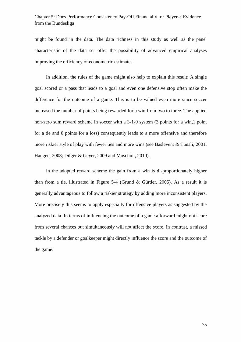
Chapter 5: Does Performance Consistency Pay-Off Financially for Players? Evidence
from the Bundesliga
75
might be found in the data. The data richness in this study as well as the panel
characteristic of the data set offer the possibility of advanced empirical analyses
improving the efficiency of econometric estimates.
In addition, the rules of the game might also help to explain this result: A single
goal scored or a pass that leads to a goal and even one defensive stop often make the
difference for the outcome of a game. This is to be valued even more since soccer
increased the number of points being rewarded for a win from two to three. The applied
non-zero sum reward scheme in soccer with a 3-1-0 system (3 points for a win,1 point
for a tie and 0 points for a loss) consequently leads to a more offensive and therefore
more riskier style of play with fewer ties and more wins (see Baslevent & Tunali, 2001;
Haugen, 2008; Dilger & Geyer, 2009 and Moschini, 2010).
In the adopted reward scheme the gain from a win is disproportionately higher
than from a tie, illustrated in Figure 5-4 (Grund & Gürtler, 2005). As a result it is
generally advantageous to follow a riskier strategy by adding more inconsistent players.
More precisely this seems to apply especially for offensive players as suggested by the
analyzed data. In terms of influencing the outcome of a game a forward might not score
from several chances but simultaneously will not affect the score. In contrast, a missed
tackle by a defender or goalkeeper might directly influence the score and the outcome of
the game.
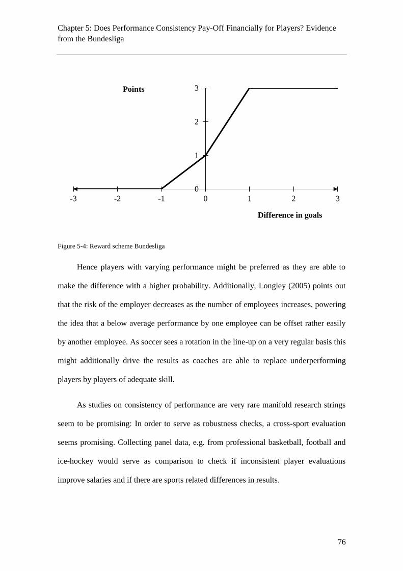
Chapter 5: Does Performance Consistency Pay-Off Financially for Players? Evidence
from the Bundesliga
76
Figure 5-4: Reward scheme Bundesliga
Hence players with varying performance might be preferred as they are able to
make the difference with a higher probability. Additionally, Longley (2005) points out
that the risk of the employer decreases as the number of employees increases, powering
the idea that a below average performance by one employee can be offset rather easily
by another employee. As soccer sees a rotation in the line-up on a very regular basis this
might additionally drive the results as coaches are able to replace underperforming
players by players of adequate skill.
As studies on consistency of performance are very rare manifold research strings
seem to be promising: In order to serve as robustness checks, a cross-sport evaluation
seems promising. Collecting panel data, e.g. from professional basketball, football and
ice-hockey would serve as comparison to check if inconsistent player evaluations
improve salaries and if there are sports related differences in results.
0
1
2
3
-3 -2 -1 0 1 2 3
Points
Difference in goals

Chapter 6: Environmental Regulations and the Relocation of Production: A Panel
Analysis of German Industry Investment Behaviour
77
6 Environmental Regulations and the Relocation of Production: A
Panel Analysis of German Industry Investment Behaviour
6.1 Introduction
Foreign Direct Investment (FDI) has risen dramatically in recent years. In 2006,
global FDI flows amounted to $1305.9 billion compared to $832.6 billion in 2001. This
represents an average growth rate of 7.79% per year. Developing economies report an
average growth rate of 10.17% per year and therefore are a major factor in this trend.
Contrary to the developing countries, developed economies only report an average
growth rate of 5.87% per year (UNCTAD, 2007). Simultaneously, with increasing FDI
flows environmentalists and ecologically-orientated academics argue that multinational
enterprises (MNE) engaged in highly polluting activities move to developing countries,
where the costs of complying with environmental standards are significantly lower.
The aim of this article is to provide new empirical evidence to the debate of the
pollution haven hypothesis and the existence of a pollution haven effect. The paper will
analyze Total German outbound FDI as well as German outbound FDI on selected
industries in the manufacturing sector and provide several novelties that have not been
applied in previous studies. Firstly, the article solely employs data from Germany rather
than data from the U.S., which was primarily used in previous studies. In addition, the
determinants of FDI are customized and specifically tailored to German outbound FDI
using the theoretical approach on FDI by Dunning (1988) combined with empirical
evidence from German surveys conducted by several leading institutions. In order to
control for unobserved country heterogeneity in the empirical analysis the study applies
a panel data set to analyse German FDI flows from 2000 to 2006. To test whether there

Chapter 6: Environmental Regulations and the Relocation of Production: A Panel
Analysis of German Industry Investment Behaviour
78
is a statistically significant relationship between German FDI and environmental
regulations, the study employs an environmental ranking published by the World
Economic Forum for each year of the sample period. This new approach makes it
possible to combine German outbound FDI flows with a reliable measured variable on
environmental regulations for almost every country that received German FDI.
6.2 Literature Review
The pollution haven hypothesis or pollution haven effect argues that a country
with a lower than average level of environmental regulations will find itself with a
comparative advantage in pollution-intensive production (Levinson, 2008). Therefore,
countries with low environmental monitoring and regulations will attract MNE´s
engaged in pollution-intensive production. Consequently, MNE´s will relocate their
production facilities, while countries with the comparative advantage will become
“havens” for the polluting industries. The rationale behind this sounds plausible: if it
costs money to conform to more stringent environmental requirements in developed
countries, profit maximizing firms would want to relocate their production activities
(Javorcik &Wei, 2004). Consequently, the relocation of polluting industries to
developing countries with less stringent environmental regulations would enhance
pollution; directly through an increase in the scale of economic activity and
transportation, as well as indirectly through changes in the composition of industries
(Brunnermeier & Levinson, 2004).
However, the findings in the literature to date do not show a clear pattern of this
effect. Xing and Kolstad (2002) conducted an empirical study by examining the FDI of
6 U.S. manufacturing industries in 1985 and 1990. Their cross-section data set covers
Chapter 6: Environmental Regulations and the Relocation of Production: A Panel
Analysis of German Industry Investment Behaviour
79
22 countries including 7 developing countries and 15 developed countries. In order to
measure environmental regulation, Xing and Kolstad (2002) used sulfur dioxide (SO2)
emissions in the host countries. The results show that host country emissions have an
insignificant effect on FDI. Once the study uses instrumental variables for SO2 (infant
mortality and population density) the results change dramatically. The results show that
predicted host country emissions have a significant negative effect on FDI in high
polluting industries. The effect suggests that for polluting industries, more lax
environmental regulations do tend to attract foreign investment.
A different conclusion is provided by Eskeland and Harrison (2003). Their study
focuses on the relationship between pollution abatement costs and the pattern of foreign
investment. The study investigated inbound FDI in 4-digit sectors in Côte d´Ivoire
(1977-1987), Morocco (1985-1990), Venezuela (1983-1988), and Mexico (1984-1990)
as well as U.S. outbound investment by sector. In order to measure pollution intensity
the study used data on U.S. pollution abatement capital expenditures and operating costs
from the PACE survey as well as data from the Industrial Pollution Projection System
(IPPS).20
The results show an insignificant effect of pollution abatements costs and U.S.
outbound FDI. Hence, the authors conclude that U.S. outbound FDI is highest in sectors
with low abatement costs (Eskeland & Harrison, 2003). Based on these results, there is
no evidence for the pollution haven hypothesis. De Santis and Stähler (2009) studied the
effect of FDI on environmental policy stringency in a two country model with trade
costs. Their results revealed if FDI is liberalized it does not lead to ecological dumping
and is more likely to occur in the absence of FDI.
20
The data comes from the U.S. Bureau of Census, Center for Economic Studies and was conducted by a
World Bank research project in order to infer the level of industrial pollution in foreign countries.

Chapter 6: Environmental Regulations and the Relocation of Production: A Panel
Analysis of German Industry Investment Behaviour
80
Javorcik and Wei (2004) examined inbound FDI in transition economies in Eastern
Europe and the former Soviet Union from multiple countries. The study used firm-level
data rather than industry-level data. Therefore, the FDI data comes from a data set based
on the results from a foreign investment survey conducted in 1995 for the period 1989-
1994. The fixed-effects regression analysis show some evidence that countries with less
stringent environmental regulations (only taken for participation in treaties) are
attracting more FDI. But the findings are not robust. Furthermore, the authors stated that
there is no evidence suggesting that multinationals in pollution-intensive activities are
more likely to invest in locations with weaker environmental standards (Javorcik &
Wei, 2004).
Cole and Elliot (2005) tried to explain the missing evidence for pollution havens
by taking the role of factor endowments in the decision of an MNE to relocate or set up
a plant in a foreign country into account. Their results indicate that Brazil and Mexico
are two of the more likely contenders to do so. Furthermore, Cole and Elliot (2005)
analysed U.S. multi-sector outbound FDI to Brazil and Mexico for the period 1989-
1994 at the three-digit U.S. SIC level of industry aggregation. Their independent
variables to determine outbound FDI to Brazil and Mexico include the physical capital
intensity of each sector, the sectors pollution abatement costs, market size, the wage
differential between the U.S. and Brazil/Mexico, R&D expenditures, a proxy for
economies of scale, and distance. By using fixed effects and random effects
specifications the results show that pollution abatement costs in a U.S. industry is a
statistically significant determinant of that industry’s FDI to Brazil and Mexico
indicating evidence of a pollution haven effect (Cole & Elliot, 2005).

Chapter 6: Environmental Regulations and the Relocation of Production: A Panel
Analysis of German Industry Investment Behaviour
81
Wagner and Timmins (2009) investigated German outbound FDI flows by German
manufacturing firms into different destination countries between 1996 and 2003. The
study analysed 6 different manufacturing industries and used a two-step econometric
procedure that explicitly controls for agglomeration effects and unobserved
heterogeneity between countries. To determine environmental stringency the authors
used a survey measure of environmental stringency developed by the World Economic
Forum and published in the Global Competitiveness Report. Additional independent
variables for the host country include accumulated FDI stock, GDP, corporate income
tax, the exchange rate, the level of tariff protection, the literacy rate, tuberculosis cases,
and distance. Wagner and Timmins (2009) results show statistically and economically
significant evidence that more stringent environmental regulation deters FDI in the
chemical industry. Consequently, this is interpreted as evidence of a pollution haven
effect for the chemical industry (Wagner & Timmins, 2009).
Spatareanu (2007) analysed data on new subsidiaries established in 16 Western
European and 9 Central and Eastern European countries by the largest 10,000 firms
operating in Europe during 1998 to 2001. By using the fixed effects logit and the Tobit
specifications the results show that stronger environmental rules in the firm’s home
economy relative to the host country are associated with a higher volume of FDI.
Furthermore, industries with higher abatement costs are likely to undertake more FDI.
However the results do not indicate that polluting industries are attracted more to
countries with weaker environmental standards.
There are several drawbacks in the existing literature that might have masked a
pollution haven effect. In order to identify a pollution effect it is essential to apply a
Chapter 6: Environmental Regulations and the Relocation of Production: A Panel
Analysis of German Industry Investment Behaviour
82
measure of environmental stringency as a variable. To measure environmental
stringency, researchers have used a variety of variables or proxies in the literature. One
reason is that there is almost no data set that covers a long time period measuring the
environmental stringency of various countries. Especially lower advanced economies do
not publish a large amount of data on emissions or environmental stringency. Most of
the existing literature therefore relies on U.S. data or solely analysed U.S. FDI and trade
flows. Particularly the earlier studies solely examined plant births in the U.S. or inbound
or outbound FDI from or into the U.S.. Furthermore, the literature identified two major
drawbacks on the methodology of studies. On the one hand, earlier studies only used
cross-sectional data. These studies tend to reject the existence of a pollution haven
effect. The major drawback of using cross-sectional data is that it is not possible to
control for unobserved attributes of countries or industries that are correlated with
regulatory stringency and economic strength (Brunnermeier & Levinson, 2004). A
country with an unobserved comparative advantage in a polluting good is likely to
export that good and enact strict environmental regulations. The simplest solution to the
problem of unobserved heterogeneity is to apply a panel data set and include fixed or
random effects by country. These fixed or random effects models capture the
unobserved characteristics of countries that make them likely to have both strict
environmental regulations and high levels of activity (Levinson, 2008). On the other
hand, an econometric issue confronting most of the studies is that economic activity and
pollution regulations may be determined simultaneously. The pollution haven
hypothesis suggests that environmental regulations affect exports, but the reverse may
also be true; exports may affect regulation. Therefore, the econometric model has to be
adjusted for endogeneity. In order to solve the problem of potential endogeneity the
Chapter 6: Environmental Regulations and the Relocation of Production: A Panel
Analysis of German Industry Investment Behaviour
83
study uses a subjective measure of environmental stringency. Furthermore, we use
random-effects instead of a fixed-effects model due to the fact that some of our
independent variables, e.g. distance, are time-invariant.
6.3 Empirical Model
Germany is an attractive country for testing the pollution haven hypothesis for
numerous reasons. Firstly, Germany is the country with the most severe and strict
environmental standards and regulations (World Economic Forum et al., 2000-2006).
Furthermore, through the central location, German firms have a large pool of possible
destinations to invest that are located close to Germany but significantly differ in
country attributes such as market size, wages, country risk and/or in environmental
stringency (Wagner & Timmins, 2009). This suggests that, ceteris paribus, pollution
intensive industries in Germany have a stronger incentive to set up production facilities
in foreign destinations than they do in most other countries in the world. Hence, we
expect to find a negative relationship between German outbound FDI and
environmental regulations. This implies that German companies prefer to invest in
countries with low environmental regulations. Consequently, this leads to the first
hypothesis:
Hypothesis 1: Host countries that have lower environmental regulations compared to
Germany will attract significantly higher German outbound FDI.
Furthermore, the German manufacturing industry is highly competitive and
accounts for 30% of Germany’s gross value creation and employs 26% of the German
workforce (Statistisches Bundesamt, 2008). This also affects the pattern of German FDI
which is rather concentrated. There are four major industries that are responsible for
Chapter 6: Environmental Regulations and the Relocation of Production: A Panel
Analysis of German Industry Investment Behaviour
84
approximately 80% of the undertaken FDI within the manufacturing industry, i.e.
automotive, chemical, electric, and engineering. By distinguishing between “clean” and
“dirty” industries we expect that the tendency to shift production to countries with lower
environmental standards is more pronounced for dirty industries. Hence, the second
hypothesis results to:
Hypothesis 2: “Dirty” industries will show a negative statistically significant
effect between FDI and environmental regulations. In contrast, the defined “clean”
industries will not present a negative statistically significant effect.
Besides that, the study expects to find a positive relationship between FDI and the
variables Gross Domestic Product per Capita (GDPPC), population, the KOF index of
globalisation, innovation, government effectiveness, as well as labour market flexibility.
These expected positive relationships, expressed through a positive statistically
significant coefficient in the regression analysis, would indicate that German outbound
FDI is attracted. Furthermore, the study expects to find a negative relationship between
FDI and the variables distance, inflation, and labour costs.
This negative relationship, expressed through a negative statistically significant
coefficient, will deter German outbound FDI in host countries. By including all the
variables in the estimation the following equation is obtained:
ln 𝐹𝐷𝐼𝑖,𝑡 = 𝛽0 + 𝛽1ln 𝐺𝐷𝑃𝑃𝐶𝑖,𝑡 + 𝛽2ln 𝑃𝑂𝑃𝑖,𝑡 + 𝛽3ln𝐷𝐼𝑆𝑇 + 𝛽4𝐼𝑁𝐹𝐿𝑖,𝑡 +
𝛽5𝐼𝑁𝑁𝑂𝑉𝐴𝑇𝐼𝑂𝑁𝑖,𝑡 +𝛽6𝐾𝑂𝐹𝑖,𝑡 + 𝛽7𝐹𝐿𝐸𝑋𝑖,𝑡 + 𝛽8𝑊𝐴𝐺𝐸𝑖,𝑡 + 𝛽9𝑆𝑇𝑅𝐼𝑁𝐺𝐸𝑁𝐶𝑌𝑖,𝑡 +
𝛽10𝐺𝑂𝑉𝑖,𝑡 + 𝛽11𝑂𝐸𝐶𝐷 + 𝜔𝑖,𝑡 (1)
Where i denotes country and t denotes year.

Chapter 6: Environmental Regulations and the Relocation of Production: A Panel
Analysis of German Industry Investment Behaviour
85
6.4 Panel Data Description
For testing the pollution haven hypothesis we use German FDI flows panel data
by destination country as well as German FDI flows by country and four major
industries from the manufacturing sector as the dependent variable.21
Data was taken
from the Deutsche Bundesbank which publishes data on Total outbound FDI from the
industries as well as breaks down outbound FDI within the manufacturing industry into
four major sectors.22
Unfortunately, the Deutsche Bundesbank does not publish further
data on other branches within the manufacturing industry and their outbound FDI. The
sample for Total outbound FDI comprises flow data for the period from 2000 to 2006
and covers all 89 destination countries that are included in the Deutsche Bundesbank
report. Due to data constraints 39 countries are included in the sample for Total German
outbound FDI.23
The country coverage for the industry samples is limited since the
Deutsche Bundesbank provides less data on the industry level. Therefore, the sample for
the chemical, automobile, electrical, and engineering industry consists of 35 countries.
In line with the current literature we use pollution abatement expenditures to
classify industries according to their pollution intensity (Wagner & Timmins, 2009). An
industry with high pollution abatement expenditures is expected to have a larger
incentive to set up production facilities abroad. In addition, the higher the share of
investments in pollution abatement on total investments, the more an industry faces a
21
German enterprises and households are required by law to report all direct and indirect holdings of 10%
or more of the capital shares or voting rights in a foreign company which has a balance sheet total of
more than three million Euros or the equivalent of three million Euros in a different currency. In addition,
all branch offices or permanent establishments in a foreign country with operating assets of three million
Euros or more have to be reported to the Deutsche Bundesbank. 22
The industries and their WZ 2008 codes are C20 – manufacture of chemicals and chemical products
(chemical), C27 – manufacture of electrical machinery and apparatus (electrical), C28 - manufacture of
machinery and equipment not elsewhere classified (engineering), and C29 – manufacture of motor
vehicles, trailers and semi-trailers (automobile). 23
In particular, Bermuda, Cayman Islands, Guernsey, Isle of Man, Jersey, Liechtenstein, Saudi Arabia,
Zambia, and Zimbabwe were excluded from all samples.

Chapter 6: Environmental Regulations and the Relocation of Production: A Panel
Analysis of German Industry Investment Behaviour
86
cost disadvantage in countries with strict environmental regulations. The data is
collected by the German Federal Bureau of Statistics (Statistisches Bundesamt) and is
available from 2002 to 2005.24
Figure 6-1 shows that the chemical industry has the
highest share of pollution abatement investment in total investment. The average share
for the chemical industry per year is 6.15% between 2002 and 2005. The mean for the
total manufacturing industry is 2.82% over this time period. Based on this data, the
cleanest industry in the sample is the electrical industry with 0.8% followed by the
engineering industry with 1.05%. The second most polluting industry is the automobile
industry with 1.72%, slightly under the mean for the total manufacturing industry.
Figure 6-1: The share of pollution abatement investment in total investment25
In order to capture the effects of the stringency of environmental regulations
(STRINGENCY) of German FDI flows, the study uses a variable taken from the Global
Competitiveness Report (GCR) published by the World Economic Forum (Spatareanu,
24
The German Federal Bureau of Statistics publishes the data in its “Fachserie 19, Reihe 3.1 Investitionen
für den Umweltschutz im Produzierenden Gewerbe”. 25
Own calculation based on data from the German Federal Bureau of Statistics (Fachserie 19, Reihe 3.1).
0
1
2
3
4
5
6
7
8
2002 2003 2004 2005
%
Year
Chemicals Engineering Automobile Electrical Manufacturing

Chapter 6: Environmental Regulations and the Relocation of Production: A Panel
Analysis of German Industry Investment Behaviour
87
2007; Wagner & Timmins, 2009).26
There are various advantages of using the GCR
index. Most of the indices used in previous studies lack on country coverage and were
not available on an annual basis. This is one reason that previous studies could not
control for unobserved heterogeneity by applying a panel data set. Instead, most studies
relied on U.S. pollution abatement data that appears to be endogenous. The GCR index
can overcome such drawbacks since it is a subjective measure of environmental
stringency determined by leading decision makers who decide on FDI flows. In
addition, the GCR ranking is available for all countries in the sample and covers the
time period of 2000 until 2006.
Apart from analyzing the effect of environmental stringency we will control for
several other variables, i.e. market size, host country wages, transportation costs, FDI
restrictions, institutional quality, innovation, country risk, and labour market flexibility.
In order to determine the market size the study uses GDP (constant prices in U.S.
Dollars) in each country in the years 2000-2006. The theoretical link between market
size and FDI is that FDI is supposed to be attracted by larger and more profitable
markets. To lessen the effect of large outliers the study applies the logarithm of GDP.
The variable comes from the World Economic Outlook Database 2008 provided by the
International Monetary Fund (IMF). Host country wages can be best measured and
compared through data on hourly compensation rates in various countries.
Unfortunately, data on labour costs and specifically data for hourly compensation rates
in various countries is very scarce since not all countries included in the sample report
26
In order to measure environmental stringency the GCR survey asked respondents the following
question: “Is the stringency of overall environmental regulations lax compared to most other countries or
among the worlds most stringent?” Business executives had to rank their country on a scale between 7 for
countries with the most stringent environmental regulations and 1 for the countries with the most lax
environmental regulations.

Chapter 6: Environmental Regulations and the Relocation of Production: A Panel
Analysis of German Industry Investment Behaviour
88
statistics to a labour organisation or to a central agency. Especially, non-member
countries of the EU or OECD do not report these data. Therefore, hourly compensation
rates (WAGE) are solely available for 42 countries in the sample.27
The proxy for
transportation costs is the direct-distance (DIST) between the source countries capital
(Berlin) and the capital of the host country in kilometers. The assumption is that the
closer a country is located to the source country, the lower the transportation costs.
FDI is also affected by the extent of openness (OPENESS) of an economy. In
order to control for this we use KOF Index of Globalisation developed by Dreher (2006)
and updated by Dreher, Gaston, and Martens (2008). The KOF index covers the
economic, social and political dimensions of globalisation. The assumption is that a
country with a high ranking in the KOF index will be more attractive for receiving more
FDI. The determinant institutional quality is covered through a government indicator
(GOV) in the host countries provided by the World Bank. The study assumes that a
higher value corresponds to better governance outcomes and therefore will attract
German outbound FDI. We furthermore assume that the relocation of production is also
driven by the innovative environment host countries offer. In particular, technology-
intensive firms tend to invest in locations with high agglomeration in order to profit
from spillovers. Hence, we assume that shifting production to foreign locations is also
affected by the pursuit to perform R&D activities and to profit from firm spillovers. To
control for this we use OECD patent data, i.e. how many patents foreign firms hold in
27
In the data set for the manufacturing industries data is missing for Turkey, Malaysia, India, Argentina,
and for the Russian Federation. In addition, the data comes from various sources namely the U.S.
Department of Labour, Bureau of Labour statistics (BLS), Eurostat (covering data for Romania, Slovenia,
and Latvia), and the data for China comes from a special report published by the BLS. Additionally, data
from China is only available from 2002-2004. The compensation rates published in Euros (Eurostat) were
converted into U.S. Dollars using annual average exchange rates taken from the International Financial
Statistics.

Chapter 6: Environmental Regulations and the Relocation of Production: A Panel
Analysis of German Industry Investment Behaviour
89
that particular host country. To account for the determinant country risk the study uses
the annual percent change of average consumer prices expressed through the inflation
rate (INFL). The data is available for all countries and all years in the sample and also
comes from the IMF World Economic Outlook database. A higher inflation rate would
indicate political instability and hence a greater country risk. A higher value would
indicate a lower country risk. In general, it is assumed that a higher country risk would
be a deterrent for FDI expressed through high annual changes in the inflation rate.
Finally, to control for labour market flexibility and regulations we use a proxy for the
Flexibility in Hiring and Firing Practices also from the GCR (2000-2007). It is assumed
that FDI is attracted by countries with more flexible labour market regulations. Table 6-
1 provides an overview and definition of the applied variables.

Chapter 6: Environmental Regulations and the Relocation of Production: A Panel
Analysis of German Industry Investment Behaviour
90
Table 6-1: Overview and definition of variables
Variables Definition Source Proxy for Author(s)
FDI Total amount of FDI from
Germany to various destination countries in €. Expressed in
logarithmic form
Statistisches Bundesamt
Sonderveröffentlichung 10,
“Bestandserhebung über Direktinvestitionen”
Dependent
Variable
Xing & Kolstad
(2002) Eskeland &
Harrison (2003)
Cole & Elliot (2005)
Wagner &
Timmins (2007) GDP (GDP) GDP at current prices in US$.
Expressed in logarithmic form
International Monetary
Fund: World Economic
Outlook Database 2008
Market size Xing & Kolstad
(2002)
Javorcik & Wei (2004)
Wagner &
Timmins (2007) Spatareanu (2007)
Distance (DIST) The distance between the host
country capital to the destination country capital as the crow flies
in km. Expressed in logarithmic
form
Transportation
costs
Javorcik & Wei
(2004) Cole & Elliot
(2005)
Wagner & Timmins (2007)
Inflation rate (INFL) Annual change. Expressed in percentages
International Monetary Fund
World Economic Outlook Database 2008
Country risk
INNOVATION Patents hold by foreign firms in
particular host country
OECD R&D
Governance (GOV) Ranges from -2.5 to 2.5, with higher values corresponding to
better governance outcomes
World Bank Institutional quality
KOF Index of
Globalisation (KOF)
Higher values denote more
globalisation
Dreher (2006): Does
Globalisation Affect Growth? Evidence from a
new Index of Globalisation,
Applied Economics 38, 10: 1091-1110.
FDI restriction
in host countries
Global
Competitiveness
Report (GCR) flexibility in hiring
and firing practices
“Flexibility” (FLEX)
Ranges from 7 for most flexible
regulations, to 1 for most rigid
Global Competitiveness
Report 2000 - 2007
Labour market
flexibility
Spatareanu (2007)
GCR stringency of environmental
regulations
(STRINGENCY)
Ranges from 7 for most stringent, to 1 for most lax
Global Competitiveness Report 2000 - 2007
Environmental stringency
Wagner & Timmins (2007)
Spatareanu (2007)
Labour costs (WAGE) Annual Labour compensation per employee (PPP) in US$
Source OECD Database/Eurostat Database
Host country wages
Eskeland & Harrison (2003)
Cole & Elliot
(2005)
OECD Equal to 1 if country is member
and 0 otherwise
CIA The World Factbook Cave & Blomquist
(2008)

Chapter 6: Environmental Regulations and the Relocation of Production: A Panel
Analysis of German Industry Investment Behaviour
91
Table 6-2 provides an overview of the descriptive statistics of the data sample. As
mentioned above, data for labour costs and especially data on hourly compensation rates
in various countries is very scarce. Therefore, the variable WAGE is limited to 283
observations. The KOF Index did not include Hong Kong and Taiwan and due to a
missing value in the Deutsche Bundesbank report from the Philippines in 2006, the total
number of observations is 268.
Table 6-2: Descriptive Statistics Total German outbound FDI
Variable Observations Mean Std. Dev. Min Max
lnFDI 268 8.221 1.933 3.258 12.22
lnGDP 269 19.082 1.671 15.543 23.303
lnDIST 269 7.460 1.164 5.662 9.806
INFL 269 3.526 4.205 -1.08 45.66
INNOVATION 269 96.49 227.36 0 1201
KOF 269 74.88 11.739 50.51 93.65
FLEX 269 3.594 0.921 1.9 6.3
WAGE 269 14.32 9.707 0.57 41.05
STRINGENCY 269 5.117 0.985 2.8 6.7
GOV 269 1.251 0.745 -0.352 2.341
OECD 287 0.658 0 1
6.5 Empirical Results
6.5.1 Descriptive Statistics
Before turning to the empirical results, we will give an overview of important
descriptive findings in the data set. This includes the question of whether German
industries in the sample with high pollution abatement expenditures are likely to
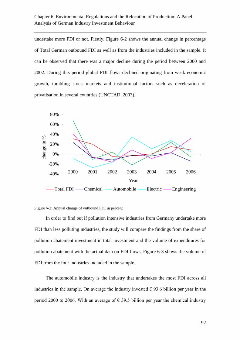
Chapter 6: Environmental Regulations and the Relocation of Production: A Panel
Analysis of German Industry Investment Behaviour
92
undertake more FDI or not. Firstly, Figure 6-2 shows the annual change in percentage
of Total German outbound FDI as well as from the industries included in the sample. It
can be observed that there was a major decline during the period between 2000 and
2002. During this period global FDI flows declined originating from weak economic
growth, tumbling stock markets and institutional factors such as deceleration of
privatisation in several countries (UNCTAD, 2003).
Figure 6-2: Annual change of outbound FDI in percent
In order to find out if pollution intensive industries from Germany undertake more
FDI than less polluting industries, the study will compare the findings from the share of
pollution abatement investment in total investment and the volume of expenditures for
pollution abatement with the actual data on FDI flows. Figure 6-3 shows the volume of
FDI from the four industries included in the sample.
The automobile industry is the industry that undertakes the most FDI across all
industries in the sample. On average the industry invested € 93.6 billion per year in the
period 2000 to 2006. With an average of € 39.5 billion per year the chemical industry
-40%
-20%
0%
20%
40%
60%
80%
2000 2001 2002 2003 2004 2005 2006
chan
ge
in %
Year
Total FDI Chemical Automobile Electric Engineering
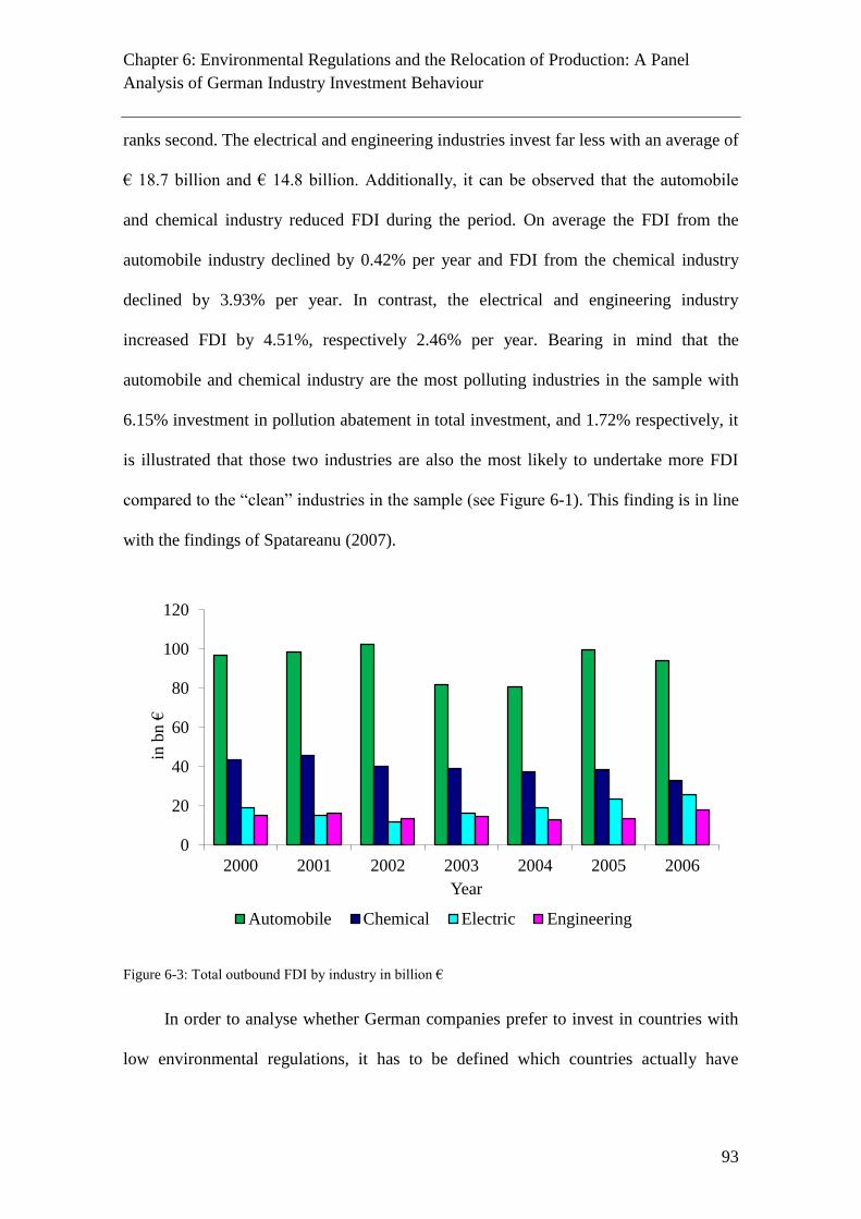
Chapter 6: Environmental Regulations and the Relocation of Production: A Panel
Analysis of German Industry Investment Behaviour
93
ranks second. The electrical and engineering industries invest far less with an average of
€ 18.7 billion and € 14.8 billion. Additionally, it can be observed that the automobile
and chemical industry reduced FDI during the period. On average the FDI from the
automobile industry declined by 0.42% per year and FDI from the chemical industry
declined by 3.93% per year. In contrast, the electrical and engineering industry
increased FDI by 4.51%, respectively 2.46% per year. Bearing in mind that the
automobile and chemical industry are the most polluting industries in the sample with
6.15% investment in pollution abatement in total investment, and 1.72% respectively, it
is illustrated that those two industries are also the most likely to undertake more FDI
compared to the “clean” industries in the sample (see Figure 6-1). This finding is in line
with the findings of Spatareanu (2007).
Figure 6-3: Total outbound FDI by industry in billion €
In order to analyse whether German companies prefer to invest in countries with
low environmental regulations, it has to be defined which countries actually have
0
20
40
60
80
100
120
2000 2001 2002 2003 2004 2005 2006
in b
n €
Year
Automobile Chemical Electric Engineering

Chapter 6: Environmental Regulations and the Relocation of Production: A Panel
Analysis of German Industry Investment Behaviour
94
relatively low environmental regulations compared to Germany (GCR 2000-2006). The
mean value for Germany during the period 2000 to 2006 is 6.64 on a scale ranging from
1 to 7, where 7 indicates the most severe regulations. This is also the highest value
across all countries in the sample. The mean value across all countries in the sample is
4.28. Therefore, we define all countries with a value under the mean of 4.28 as countries
with low environmental regulations compared to Germany. This splits the sample into
42 low regulated countries and 38 countries with strict environmental regulations. By
adding the annual growth rate of German outbound FDI in relation to the environmental
stringency of the two groups it is possible to observe which group has the highest
annual growth rates of receiving German outbound FDI.
Figure 6-4: German FDI growth rates of countries with low/strict regulations
Figure 6-4 shows that the growth rates of low regulated countries outperform the
growth rates of the strict regulated countries in almost every year. Solely during the
downturn in 2002 and 2003, strict regulated countries had slightly higher growth rates
-20%
0%
20%
40%
60%
80%
100%
2000 2001 2002 2003 2004 2005 2006
Annual
gro
wth
in %
Year Low regulated Strict regulated
Linear (Low regulated) Linear (Strict regulated)
Chapter 6: Environmental Regulations and the Relocation of Production: A Panel
Analysis of German Industry Investment Behaviour
95
compared to low regulated countries. The green trend line clearly shows that countries
with low regulations have a positive linear trend in the sample period, whereas the red
trend line shows a negative trend for the strict regulated countries. This illustration only
takes the growth rates in relation to the environmental stringency of a country on a
yearly basis into account but excludes all other factors such as volume of FDI or other
explanatory variables that might explain FDI flows.
6.5.2 Empirical Results on an aggregated level
The results of the panel regression on an aggregated level are shown in Table 6-
3.28,29
In particular, the results show that six out of the eleven variables are statistically
significant. The variable for market size GDP is significant at the 1% level. The variable
DIST shows the expected sign, which means that economies in proximity to Germany
attract German FDI, and is statistically significant at the 1% level. The FLEX shows a
negative sign but is not significant. The KOF globalisation index doesn’t have the
expected sign but is at the same time not statistically significant in this analysis. The
variable for Innovation is not significant whereas the variable for institutional quality
(GOV) shows the expected sign and is significant at the 5% level. The variable WAGE
is highly significant at the 1% level and has the expected negative sign. The negative
sign confirms the assumption that German outbound FDI is attracted to countries with
lower labour costs or countries with lower hourly compensation rates. The mean value
for hourly compensation rates in Germany is $28.58 per hour, which differs strongly
28
In general, panel regressions suffer from non-stationarity. In order to check whether the panel shows
non-stationarity we applied the Augmented Dickey-Fuller test for each independent variable. There were
no signs of non-stationarity. 29
The Wald chi2 test also indicates that the model itself is highly significant and that all variables should
be included in the model. We have also controlled for the issue of multicollinerarity. An examination of
the correlations of the independent variables revealed that multicollinearity is not exerting an undue
influence on the results. Also, the corresponding variance inflation factors (VIF) do not reach critical
values.
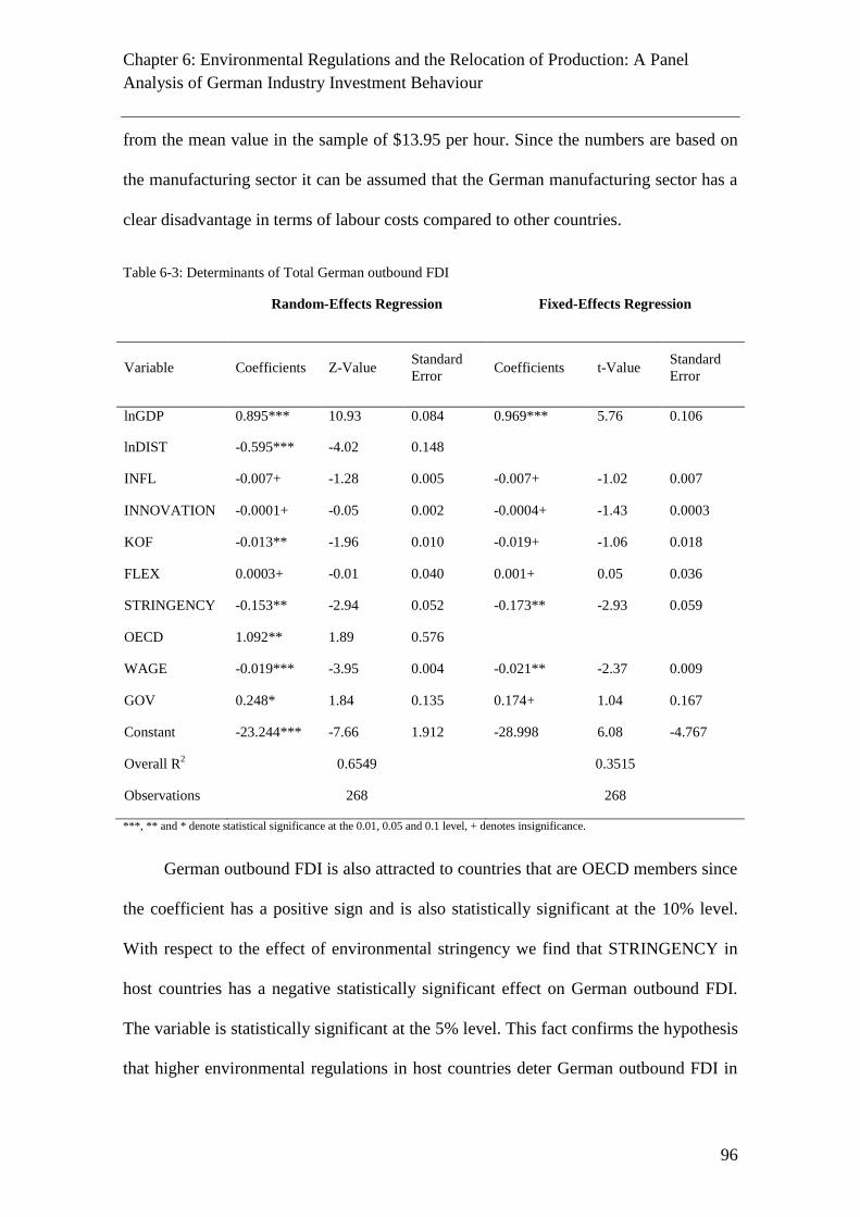
Chapter 6: Environmental Regulations and the Relocation of Production: A Panel
Analysis of German Industry Investment Behaviour
96
from the mean value in the sample of $13.95 per hour. Since the numbers are based on
the manufacturing sector it can be assumed that the German manufacturing sector has a
clear disadvantage in terms of labour costs compared to other countries.
Table 6-3: Determinants of Total German outbound FDI
Random-Effects Regression Fixed-Effects Regression
Variable Coefficients Z-Value Standard
Error Coefficients t-Value
Standard
Error
lnGDP 0.895*** 10.93 0.084 0.969*** 5.76 0.106
lnDIST -0.595*** -4.02 0.148
INFL -0.007+ -1.28 0.005 -0.007+ -1.02 0.007
INNOVATION -0.0001+ -0.05 0.002 -0.0004+ -1.43 0.0003
KOF -0.013** -1.96 0.010 -0.019+ -1.06 0.018
FLEX 0.0003+ -0.01 0.040 0.001+ 0.05 0.036
STRINGENCY -0.153** -2.94 0.052 -0.173** -2.93 0.059
OECD 1.092** 1.89 0.576
WAGE -0.019*** -3.95 0.004 -0.021** -2.37 0.009
GOV 0.248* 1.84 0.135 0.174+ 1.04 0.167
Constant -23.244*** -7.66 1.912 -28.998 6.08 -4.767
Overall R2 0.6549 0.3515
Observations 268 268
***, ** and * denote statistical significance at the 0.01, 0.05 and 0.1 level, + denotes insignificance.
German outbound FDI is also attracted to countries that are OECD members since
the coefficient has a positive sign and is also statistically significant at the 10% level.
With respect to the effect of environmental stringency we find that STRINGENCY in
host countries has a negative statistically significant effect on German outbound FDI.
The variable is statistically significant at the 5% level. This fact confirms the hypothesis
that higher environmental regulations in host countries deter German outbound FDI in
Chapter 6: Environmental Regulations and the Relocation of Production: A Panel
Analysis of German Industry Investment Behaviour
97
those countries. Additionally, this result provides evidence for a “pollution haven
effect” in German outbound FDI. To express the result in relation to each other and to
show how important the result is economically, the result can be described as semi-
elasticity. This means that, all else being equal, a change by one unit in environmental
regulations by a certain country (e.g. from 3 to 4) will cause a decrease of
approximately 15% of receiving German FDI. In summary, German companies
investing abroad seem to take the costs through differences in environmental regulations
across various countries into account. Consequently, German companies try to
circumvent the additional costs in order to comply with environmental regulations in
Germany by investing more in lower regulated countries and relocating production
facilities towards these countries.
In order to support this result and to provide evidence for a “pollution haven
effect” in the manufacturing sector the article will also outline FDI patterns on the
industry level.
6.5.3 Empirical Results on the industry level
Since data on the industry level is very scarce in terms of country coverage and
therefore the number of observations is relatively low, the study will apply a different
empirical model for all regression analyses on the industry level. The results obtained
from applying a random effects or fixed effects model did not show any significant
results due to relatively low number of observations. All independent variables used in

Chapter 6: Environmental Regulations and the Relocation of Production: A Panel
Analysis of German Industry Investment Behaviour
98
the regressions were insignificant and could not be interpreted. Therefore, the data on
the industry level will be analysed by using the OLS technique.30
The chemical industry is one of the industries defined as a “dirty” industry. This
was outlined based on the industries expenditures for pollution abatement. Therefore,
the chemical industry is the industry which is most likely to show a “pollution haven
effect”. Furthermore, the descriptive statistics indicate that the countries in the sample
are on average more advanced economies.31
The empirical results from the
manufacturing industries are shown in Table 6-4.
The results from the regression analysis for the chemical industry confirm the
previous results from the Total German outbound FDI sample. Again, GDP is highly
significant at the 1% with a positive coefficient. The variable DIST and FLEX are both
significant and also show the expected sign. INFL is significant at the 1% level and has
a negative sign. This means that companies in the German chemical industry are
attracted to secure markets with a low country risk. This is also confirmed through the
KOF index which is statistically significant at the 1% level and shows a positive sign
indicating that low trade barriers and openness towards globalisation is an important
determinant for the German chemical industry.
30
The major drawback of this technique is that it is not possible to control for unobserved heterogeneity
and therefore the results may be biased as discussed earlier. 31
The relatively high mean value on the globalization index shows that more advanced economies are
included in the sample. In addition, data on the KOF index for Hong Kong as well as data on FDI flows
to Romania and Slovakia for 2000 is not available. Moreover, there is no available data on labour costs in
China for the years 2000, 2001, 2005 and 2006. For that reason, China was dropped for the years of
missing data. Additionally, Hong Kong was completely dropped from the sample and Romania and Slovakia were dropped for the year 2000.Therefore, the total number of observations is 190 in the sample
for the chemical industry.
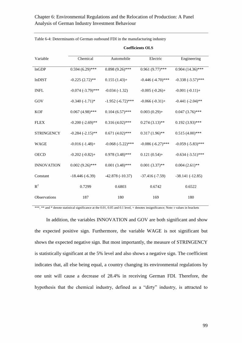
Chapter 6: Environmental Regulations and the Relocation of Production: A Panel
Analysis of German Industry Investment Behaviour
99
Table 6-4: Determinants of German outbound FDI in the manufacturing industry
Coefficients OLS
Variable Chemical Automobile Electric Engineering
lnGDP 0.594 (6.29)*** 0.898 (9.26)*** 0.961 (9.77)*** 0.904 (14.36)***
lnDIST -0.225 (2.72)** 0.155 (1.43)+ -0.446 (-4.70)*** -0.338 (-3.57)***
INFL -0.074 (-3.79)*** -0.034 (-1.32) -0.005 (-0.26)+ -0.001 (-0.11)+
GOV -0.340 (-1.71)* -1.952 (-6.72)*** -0.066 (-0.31)+ -0.441 (-2.04)**
KOF 0.067 (4.98)*** 0.104 (6.57)*** 0.003 (0.29)+ 0.047 (3.76)***
FLEX -0.200 (-2.69)** 0.316 (4.02)*** 0.274 (3.13)** 0.192 (3.93)***
STRINGENCY -0.284 (-2.15)** 0.671 (4.02)*** 0.317 (1.96)** 0.515 (4.00)***
WAGE -0.016 (-1.48)+ -0.068 (-5.22)*** -0.086 (-6.27)*** -0.059 (-5.83)***
OECD -0.202 (-0.82)+ 0.978 (3.48)*** 0.121 (0.54)+ -0.634 (-3.51)***
INNOVATION 0.002 (9.26)*** 0.001 (3.48)*** 0.001 (3.37)** 0.004 (2.61)**
Constant -18.446 (-6.39) -42.878 (-10.37) -37.416 (-7.59) -38.141 (-12.85)
R2 0.7299 0.6803 0.6742 0.6522
Observations 187 180 169 180
***, ** and * denote statistical significance at the 0.01, 0.05 and 0.1 level, + denotes insignificance; Note: t values in brackets
In addition, the variables INNOVATION and GOV are both significant and show
the expected positive sign. Furthermore, the variable WAGE is not significant but
shows the expected negative sign. But most importantly, the measure of STRINGENCY
is statistically significant at the 5% level and also shows a negative sign. The coefficient
indicates that, all else being equal, a country changing its environmental regulations by
one unit will cause a decrease of 28.4% in receiving German FDI. Therefore, the
hypothesis that the chemical industry, defined as a “dirty” industry, is attracted to
Chapter 6: Environmental Regulations and the Relocation of Production: A Panel
Analysis of German Industry Investment Behaviour
100
countries with low environmental regulations is statistically confirmed. This further
supports the existence of a “pollution haven effect”.
The second industry defined as “dirty” in the sample is the automobile industry.
The descriptive statistics are very similar compared to the sample of the chemical.32
The
results show several surprising effects. First of all, the variable GDP, the proxy for
market size, is again highly statistically significant in this regression. The variable DIST
is not significant in this regression. On the other side, the variable FLEX in labour
markets is statistically significant at the 1% level and shows the expected sign. The
variable WAGE shows the expected sign and is highly significant. The variable GOV is
highly significant and reports a negative sign. The results show that companies in the
automobile industry are attracted to countries with closer distance, lower inflation rates,
less institutional quality but more flexible labour markets. In general, all these
determinants indicate cost savings, especially in the production process. Furthermore,
companies in the automobile industry are attracted to host countries with low trade
barriers as well as openness to globalisation, indicated through the positive and
statistically significant relationship between German FDI and the KOF index. Since the
automobile industry is defined as “dirty” in this study it was expected to find a negative
statistically significant relationship between German FDI and the STRINGENCY in
host countries. As the results show, there is a significant relationship but it does not
show the expected sign. Consequently, the second proposed hypothesis in this study
cannot be confirmed for the automobile industry. In fact, the results indicate that
companies in the automobile industry are attracted to countries with high environmental
32
Data for Luxembourg was not available for the automobile industry and is therefore not included in this
sample. Hence, the number of observations is reduced to 180.

Chapter 6: Environmental Regulations and the Relocation of Production: A Panel
Analysis of German Industry Investment Behaviour
101
regulations. This could possibly reflect a turnaround in German automotive industry’s
strategically environmental consciousness with regard to future market potential. In
particular, consumers of environmental stringent countries have developed a strong
demand for environmentally efficient products, i.e. hybrid fuel technologies which will
continue to rise in the future. An explanation provided by Rauscher (2009) states that
everything else being equal, tighter environmental standards retard rather than
accelerate long-term economic growth despite potentially substantial spill-overs in the
green R&D sector. In addition, the variable INNOVATION, highly significant and
positive, supports the result. Hence, our results give support for the Porter hypothesis
which states that environmental regulation causes cost reducing innovation and
promotes competitiveness (Porter & van der Linde, 1995).
The electric industry is the first defined as a “clean” industry in the sample.
Therefore, the paper does not expect to find a negative relationship between German
outbound FDI and environmental regulations in the host country. The results of the
regression analysis are presented in Table 6-4.33
The variable for market size GDP is
again statistically significant at the 1% level. Also the variable DIST in this regression
is significant at the 1% level and shows a negative sign. In contrast to the defined
“dirty” industries, DIST or close proximity to Germany has an influential impact on
receiving German FDI in the electric industry. The variables INFL and GOV are not
statistically significant for the electric industry. The KOF index also shows the expected
sign but slightly fails to be significant at the 10% level. Additionally, the variables
WAGE, INNOVATION and FLEX show the expected signs and are highly significant.
33
Due to data constraints for German FDI flows to Romania (2000, 2003, and 2005), Slovakia (2000,
2002), Ireland (2002) and Norway for all years in the sample period, the number of observations is
reduced to 169.

Chapter 6: Environmental Regulations and the Relocation of Production: A Panel
Analysis of German Industry Investment Behaviour
102
As expected, the variable STRINGENCY does not show a negative sign and therefore
supports the second hypothesis. In fact, the coefficient shows a positive sign and is
highly significant. As a consequence, German companies in the electric industry prefer
to invest in countries that have high environmental regulations. The second defined
“clean” industry in the sample is the engineering industry. Regarding the second
hypothesis, we expect the same findings as for the electric industry. The results are
similar to those obtained from the electric industry with the exceptions that the variables
KOF and OECD are statistically significant. The variable DIST is statistically
significant and reports a negative sign. Surprisingly, this result regarding DIST differs
from the regression results obtained from the defined “dirty” chemical industry. This
indicates that DIST is an important determinant for the “clean” industries, whereas the
contrary applies for the “dirty” industry in the sample. Consequently, it can be
maintained that firms engaged in “clean” industries prefer investment destinations close
to their home market as they move both consciously and physically up their
environmental value-added chains. One may argue, occasioned inter alia by rising
living standards and possible market enlargement effects - and partly due to changes in
their production and marketing strategies, that the DIST variable effects may now rest
more upon spatial optimization of an interrelated set of value-added activities in the
"clean" industries. In contrast, firms engaged in “dirty” industries appear to be still
adhering to more traditional motives of superficial myopic cost minimization strategies
without taking into account the mid- and long term strategic asset effects of sustaining a
“dirty” image.
The variable INNOVATION shows the expected sign and is also significant. In
addition, the variables KOF and FLEX are significant. Also firms in the engineering
Chapter 6: Environmental Regulations and the Relocation of Production: A Panel
Analysis of German Industry Investment Behaviour
103
industry are attracted to countries with lower wages compared to Germany. Concerning
the measure of STRINGENCY, the results show a positive significant relationship
between environmental stringency and German outbound FDI. Consequently, the results
confirm the second proposed hypothesis that there is no negative relationship between
German FDI and environmental regulations in host countries across “clean” industries.
6.6 Discussion
The study proposed two hypotheses in order to provide evidence for a pollution
haven effect in German outbound FDI. Therefore, the study applies an empirical model
to detect a relationship between environmental regulations and German outbound FDI.
The novelties in this study are the application of customized FDI determinants for the
source country Germany as well as the assembly of the variables in connection with the
environmental variable. The environmental variable, taken from the GCR, is a
subjective measure of environmental stringency determined by leading decision makers
who decide on FDI flows. Consequently, the environmental variable does not suffer
from potential endogeneity. In addition, the data for the GCR environmental stringency
index is available for the investigated sample period from 2000 until 2006. Therefore,
the index can be included in a panel data set and can overcome the drawbacks of
unobserved heterogeneity.
The results of the regression analysis for Total German outbound FDI are
multifarious. The results show a negative statistically significant relationship between
environmental regulations and German outbound FDI. This indicates that German FDI
is attracted to countries with lower environmental regulations. More precisely, all else
being equal, an increase by one unit in environmental regulations by a certain country

Chapter 6: Environmental Regulations and the Relocation of Production: A Panel
Analysis of German Industry Investment Behaviour
104
will cause a decrease of approx. 15% of receiving German FDI. This finding strongly
supports the first hypothesis and provides evidence for a pollution haven effect in
German outbound FDI. Consequently, the difference in environmental regulations
across countries can be seen as an important determinant in explaining German
outbound FDI. Therefore, it can be argued that German companies try to circumvent the
costs related to severe environmental regulations in Germany by investing more in
countries with lower environmental regulations and possibly shifting production
facilities towards these countries.
A major contributor of FDI in Germany is the manufacturing sector. The sector
accounts for 18% of total German outbound FDI. In order to provide further evidence
for a pollution haven effect the study also investigates German outbound FDI in various
industries in the manufacturing sector. Based on the data for the share of pollution
abatement investment in total investment, the study defines “dirty” and “clean”
industries that are included in the sample. Consequently, the second hypothesis states
that there is a negative statistically significant relationship between German outbound
FDI in “dirty” industries and environmental regulations in destination countries,
whereas the “clean” industries do not show the effect. This hypothesis is confirmed for
the chemical industry but has to be rejected for the automobile industry. An explanation
for this outcome is that the share of pollution abatement investment in total investment
in the chemical industry is approximately 3.5 times (6.15% vs. 1.72%) higher compared
to the automobile industry. This fact supports the assumption that costs related to
comply with environmental standards influence decisions on investments. This fact can
only be confirmed if the costs represent a significant fraction of the total costs. Another
explanation would be a turnaround in the demand for environmentally efficient products
Chapter 6: Environmental Regulations and the Relocation of Production: A Panel
Analysis of German Industry Investment Behaviour
105
in the automotive industry. In contrast, the defined “clean” industries do not show a
negative statistically significant effect, which further confirms the second hypothesis.
Additionally, the results support the assumption that German outbound FDI is attracted
to countries with large domestic markets as well as to countries with significantly lower
labour costs. Furthermore, in almost all regression analyses, the openness to
globalisation of a certain country is an important determinant for German outbound
FDI.
The limitation of the study is the shortage of data. Firstly, data on hourly
compensation rates or an equivalent measure of labour costs has not been significantly
published or reported by various countries. Furthermore, data on German FDI flows is
only published for a limited number of industries and countries. Due to the data
limitation, it is not possible for the study to apply an empirical model that controls for
unobserved heterogeneity on the industry level. The limited size of the data and the
imperfect coverage of the labour costs data suggest that future studies should
concentrate on expanding the data set and industries covered. It would also be
appropriate to investigate other methods of collecting FDI data, for example, to apply
firm-level data on investment decisions.
Chapter 7: Conclusion and Outlook
106
7 Conclusion and Outlook
Modern professional sport teams are complex businesses, intrinsically concerned
with matters of economics and finance (Morrow, 2003). This dissertation extracts some
managerial decisions and regulations that influence this complexity. Beginning with a
key element of the industry, namely, the league structure that is essential to the
production of the sport product, Chapter 2 demonstrates the influence of sport’s
governing bodies and the ways in which they arrange league structures. In a bid to
increase the attractiveness of the game for spectators and generate additional revenues,
European basketball leagues adopted a shorter shot clock in 2000. My empirical
analysis revealed that though this rule change may have enhanced attractiveness in
terms of scoring, it simultaneously led to decreased competitive balance, thus
establishing a trade-off between two desired outcomes. To evaluate and generalize these
results, comparable research in other sports that have adjusted their rules would be
helpful.
The next two chapters emphasize the financial performance of professional sport
teams. I first addressed whether the introduction of a new CBA improved managerial
technical efficiency, in terms of maximizing team values and revenue generation. The
average efficiencies increased by up to 9 percentage points, compared with before the
new CBA was established for the NHL, and the ten least efficient teams benefited even
more, in that their average efficiency improved up to 14 percentage points. To explicate
the surprising result that sporting performance influenced neither team values nor team
revenues, I then presented an empirical study of the differences in motives between
North American and European team sports. Athletic achievement had significant
influences on financial performance only among EPL clubs, not for teams in North

Chapter 7: Conclusion and Outlook
107
American major leagues, which supported the results from the previous chapter. In
addition, the DEA efficiency analyses indicated a predominant sporting focus among
EPL teams, whereas North American major league franchises tended to be more
business-oriented organizations. Further research might extend and confirm these
findings by analyzing whether other European sport leagues exhibit similar results with
regard to their sport and financial performance.
Beyond these insights into the impacts of decisions by governing bodies and team
owners, Chapter 5 spotlights individual players and the determinants of their
remuneration. Specifically, I tested whether performance consistency is rewarded. This
initial application of a longitudinal data set revealed findings that contradicted the
results of previous research: I found strong evidence of a salary premium for players
who perform inconsistently. Controlling for individual player characteristics and
performance indicators, a one standard deviation increase in inconsistency earned the
player a salary surplus of up to 92%, depending on the econometric model. Studies of
performance consistency are very rare, so manifold research opportunities arise from
this analysis. For example, as a robustness check, a cross-sport evaluation would be
helpful. Panel data from professional basketball, football, and hockey players could
offer a revealing comparison to determine if inconsistent player evaluations improve
salaries across the board, or if sports-related differences appear in the results.
One of the most promising research streams for sports economics relies on the
increasing availability of vast amounts of new data, as connected with the still poorly
defined term “big data.” Such data come from various sources and may not be publicly
available. For example, the NBA has equipped every arena with a data collection
system called SportVU that measures each player’s every move by analyzing optical

Chapter 7: Conclusion and Outlook
108
tracking data, recorded through several cameras throughout the arena. In one of the first
studies to analyze these data, Cervone et al. (2014) propose a new metric to measure
performance value in the NBA, in which each possession takes a value. Then the
derived value is based on the probability of a made basket, which is equal to the total
number of expected points that will result from a possession, or expected possession
value (EPV). Because the EPV assigns a point value to every tactical option available at
each moment of a possession, it can reveal the decisive moment that led to an open shot,
instead of merely capturing the open shot, a current box score metrics do. The EPV also
quantifies a player’s combined offensive value, taking into account every single action
over a given time span and summarizing it as a single value. Comparing this value
across players in turn offers a more accurate estimate of performance that might help
explain wage dispersions. For European soccer, similar data are collected by Opta
Sports. Yet a major limitation remains, in that these big data demand considerable
resources to be analyzed, and few professional sports teams employ sufficiently well-
equipped statisticians. This gap might be why Manchester City FC publicly released all
the data collected about it by Opta Sports for the entire 2012–13 season. With a
crowdsourcing model, Manchester City FC is seeking to learn how to use its data more
effectively and efficiently.
Finally, professional sport teams likely include various data sources in their
decision-making processes as they seek to optimize their operations, maximize game
day revenues, and earn more from their sponsorships and merchandise operations.
Experts and team owners highlight the benefits of WiFi-equipped arenas, which allow
teams to collect personalized, real-time data about their attendees, for segmentation and
profiling purposes. According to team owners, an average purchase includes three
Chapter 7: Conclusion and Outlook
109
tickets, which means that they collect purchase data from only about one-third of the
attendees in the arena; the other two-thirds are virtually anonymous. Data gathered from
WiFi operations could help optimize waiting queues for food and beverage vendors or
even reducing waiting times for restrooms. By exploiting such information and data,
teams can enhance the fans´ experience and increase game day revenues. An embedded
social media strategy within organizations, to collect data about fan behavior, similarly
appears increasingly imperative as a means to increase fans’ engagement.
Eventually, those professional sport teams that use data and derive analytic
insights from available data sources in the most efficient way will gain a competitive
advantage—one that ultimately might lead to superior sport and business performance.
VI
8 Bibliography
Alexander, D. L., & Kern, W. (2004). The economic determinants of professional sports
franchise values. Journal of Sports Economics, 5(1), 51-66.
Alexander, W. R. J., Haug, A. A., & Jaforullah, M. (2010). A two-stage double-
bootstrap data envelopment analysis of efficiency differences of New Zealand
secondary schools. Journal of Productivity Analysis, 34(2), 99-110.
Andersen, P., & Petersen, N. C. (1993). A procedure for ranking efficient units in data
envelopment analysis. Management Science, 39(10), 1261-1264.
Antweiler, W., Copeland, B. R., & Taylor, M. S. (2001). Is free trade good for the
environment? American Economic Review, 91(4), 877-908.
Atkinson, S. E., Stanley, L. R., & Tschirhart, J. (1988). Revenue sharing as an incentive
in an agency problem: An example from the National Football League. Rand Journal
of Economics, 19(1), 27-43.
Banker, R. D., Charnes, A., & Cooper, W. W. (1984). Some models for estimating
technical and scale inefficiencies in data envelopment analysis. Management
science, 30(9), 1078-1092.
Barney, J. (1991). Firm resources and sustained competitive advantage. Journal of
Management, 17(1), 99-120.
Barney, J. B. (1995). Looking inside for competitive advantage. Academy of
Management Executive, 9(4), 49-61.
Barros, C. P., Assaf, A., & Sá-Earp, F. (2010). Brazilian football league technical
efficiency: a Simar and Wilson approach. Journal of Sports Economics, 11(6), 641-
651.
Barros, C. P., Del Corral, J., & Garcia-del-Barrio, P. (2008). Identification of segments
of soccer clubs in the Spanish league first division with a latent class model. Journal
of Sports Economics, 9(5), 451-469.

VII
Barros, C. P., & Garcia-del-Barrio, P. (2011). Productivity drivers and market dynamics
in the Spanish first division football league. Journal of Productivity Analysis, 35(1),
5-13.
Barros, C. P., Garcia-del-Barrio, P., & Leach, S. (2009). Analysing the technical
efficiency of the Spanish football league first division with a random frontier model.
Applied Economics, 41(25), 3239-3247.
Barros, C. P., & Leach, S. (2006). Performance evaluation of the English Premier
Football League with data envelopment analysis. Applied Economics, 38(12), 1449-
1458.
Baslevent, C. & Tunali, I. (2001). Incentives and outcomes in football. Mimeo.
Battese, G. E., & Coelli, T. J. (1995). A model for technical inefficiency effects in a
stochastic frontier production function for panel data. Empirical Economics, 20(2),
325-332.
Berger, J., & Nieken, P. (2014). Heterogeneous contestants and the intensity of
tournaments: An empirical investigation. Journal of Sports Economics, DOI:
10.1177/1527002514538639.
Berri, D., & Simmons, R. (2009). Race and the evaluation of signal callers in the
National Football League. Journal of Sports Economics, 10(1), 23-43.
Bodvarsson, Ö. & Brastow, T. (1998). Do employers pay for consistent performance?
Evidence from the NBA. Economic Inquiry, 36(1), 145-160.
Brunnermeier, S. B., & Levinson, A. (2004). Examining the evidence on environmental
regulations and industry location. Journal of the Environment and Development,
13(1), 6-41.
Bryson, A., Frick, B., & Simmons, R. (2013). The returns to scarce talent: footedness
and player remuneration in European soccer. Journal of Sports Economics, 14(6),
606-628.
VIII
Büschemann, A., & Deutscher, C. (2011). Did the 2005 collective bargaining agreement
really improve team efficiency in the NHL? International Journal of Sport Finance,
6(4), 298-306.
Cain, L. P., & Haddock, D. D. (2005). Similar economic histories, different industrial
structures: transatlantic contrasts in the evolution of professional sports leagues.
Journal of Economic History, 65(4), 1116-1147.
Cave, L. A., & Blomquist, G. C. (2008). Environmental policy in the European Union:
Fostering the development of pollution havens? Ecological Economics,65(2), 253-
261.
Cervone, D., D’Amour, A., Bornn, L., & Goldsberry, K. (2014). Pointwise: Predicting
points and valuing decisions in real time with NBA optical tracking data. Paper
presented at the 2014 MIT Sloan Sports Analytics Conference.
Charnes, A., Cooper, W. W., & Rhodes, E. (1978). Measuring the efficiency of decision
making units. European Journal of Operational Research, 2(6), 429-444.
Cole, M. A., & Elliott, R. J. (2005). FDI and the capital intensity of “dirty” sectors: a
missing piece of the pollution haven puzzle. Review of Development Economics,
9(4), 530-548.
Copeland, B., & Taylor, M. S. (2004). Trade, growth and the environment. Journal of
Economic Literature, 42(1), 7-71.
Cornelius, P. (2003). The global competitiveness report 2002-2003. New York: Oxford
University Press.
Croix, S. J. L., & Kawaura, A. (1999). Rule changes and competitive balance in
Japanese professional baseball. Economic Inquiry, 37(2), 353-368.
Daft, R. (1983). Organization theory and design. New York: West.
D’Agostino, R., Balanger, A., & D’Agostino, R., Jr. (1990). A suggestion for using
powerful and informative tests of normality. American Statistician, 44(4), 316-327.
IX
Daly, G., & Moore, W. J. (1981). Externalities, property rights and the allocation of
resources in Major League Baseball. Economic Inquiry, 19(1), 77-95.
Dawson, P., Dobson, S., & Gerrard, B. (2000). Estimating coaching efficiency in
professional team sports: Evidence from English association football. Scottish
Journal of Political Economy, 47(4), 399-421.
Deloitte & Touche (2001–2009). Annual review of football finance. London, Reports
for UK.
De Santis, R. A., & Stähler, F. (2009). Foreign direct investment and environmental
taxes. German Economic Review, 10(1), 115-135.
Despotis, D. K. (2002). Improving the discriminating power of DEA: focus on globally
efficient units. Journal of the Operational Research Society, 53(3), 314-323.
Deutsche Bundesbank (2003, 2006, 2007). Bestandserhebung über Direkinvestitionen.
Statistische Sonderveröffentlichung 10, Frankfurt a.M.
Deutscher, C. & Büschemann, A. (2014, forthcoming). Does Performance Consistency
Pay Off Financially for Players? Evidence from the Bundesliga, Journal of Sports
Economics, doi: 10.1177/1527002514521428
Deutscher, C., Frick, B., Gürtler, O., & Prinz, J. (2013). Sabotage in tournaments with
heterogeneous contestants: Empirical evidence from the soccer pitch. Scandinavian
Journal of Economics, 115(4), 1138-1157.
Dietl, H. M., Grossmann, M., & Lang, M. (2011). Competitive balance and revenue
sharing in sports leagues with utility-maximizing teams. Journal of Sports
Economics, 12(3), 284-308.
Dilger, A. & Geyer, H. (2007). Theoretical and empirical analysis of the three-point-
rule. Sport and Society, 4(3), 265-277.
Dougherty, C. (2002). Introduction to econometrics, Vol. 2. Oxford: Oxford University
Press.

X
Dreher, A. (2006). Does globalization affect growth? Evidence from a new index of
globalization. Applied Economics, 38(10), 1091-1110.
Dreher, A., Gaston, N., & Martens, P. (2008). Measuring globalisation: Gauging its
consequences. Berlin: Springer.
Dunning, J. H. (1988). Explaining international production. London: Unwin Hyman.
Dunning, J. H. (Ed.). (1993). The theory of transnational corporations. London: Taylor
& Francis.
Dunning, J. H., & Lundan, S. M. (2008). Multinational enterprises and the global
economy. Cheltenham, UK: Edward Elgar Publishing.
Dyson, R. G., Allen, R., Camanho, A. S., Podinovski, V. V., Sarrico, C. S., & Shale, E.
A. (2001). Pitfalls and protocols in DEA. European Journal of Operational
Research, 132(2), 245-259.
Ederington, J., Levinson, A., & Minier, J. (2005). Footloose and pollution-free. Review
of Economics and Statistics, 87(1), 92-99.
Ederington, J., & Minier, J. (2003). Is environmental policy a secondary trade barrier?
An empirical analysis. Canadian Journal of Economics, 36(1), 137-154.
Einolf, K. W. (2004). Is winning everything? A data envelopment analysis of Major
League Baseball and the National Football League. Journal of Sports Economics,
5(2), 127-151.
El-Hodiri, M., & Quirk, J. (1971). An economic model of a professional sports league.
Journal of Political Economy, 79(6), 1302-1319.
El-Mahgary, S., & Lahdelma, R. (1995). Data envelopment analysis: Visualizing the
results. European Journal of Operational Research, 83(3), 700-710.
Eschweiler, M., & Vieth, M. (2004). Preisdeterminanten bei Spielertransfers in der
Fußball-Bundesliga - Eine empirische Analyse. Die Betriebswirtschaft, 64, 671-692.
XI
Eskeland, G. S., & Harrison, A. E. (2003). Moving to greener pastures? Multinationals
and the pollution haven hypothesis. Journal of Development Economics, 70(1), 1-23.
Espitia‐Escuer, M., & García‐Cebrián, L. I. (2010). Measurement of the efficiency of
football teams in the Champions League. Managerial and Decision Economics,
31(6), 373-386.
Fama, E. F. (1970). Efficient capital markets: A review of theory and empirical work.
Journal of Finance, 25(2), 383-417.
Fizel, J. L., & D'Itri, M. P. (1997). Managerial efficiency, managerial succession and
organizational performance. Managerial and Decision Economics, 18(4), 295-308.
Flores, R., Forrest, D., & Tena, J. D. D. (2010). Impact on competitive balance from
allowing foreign players in a sports league: Evidence from European soccer. Kyklos,
63(4), 546-557.
Forrest, D., & Simmons, R. (2002). Outcome uncertainty and attendance demand in
sport: The case of English soccer. Journal of the Royal Statistical Society: Series D,
51(2), 229-241.
Fort, R. (2000). European and North American sports differences (?). Scottish Journal
of Political Economy, 47(4), 431-455.
Fort, R. (2006). The value of major league baseball ownership. International Journal of
Sport Finance, 1(1), 9-20.
Fort, R. (2007). Comments on "Measuring Parity". Journal of Sports Economics, 8(6),
642-651.
Fort, R., Lee, Y. H., & Berri, D. (2008). Race and coaching efficiency in the NBA,
International Journal of Sport Finance, 3(2), 84-97.
Fort, R., & Quirk, J. (1995). Cross-subsidization, incentives, and outcomes in
professional team sports leagues. Journal of Economic Literature, 33(3), 1265-1299.
Franck, E., & Nüesch, S. (2008). Mechanisms of superstar formation in German soccer:
Empirical evidence. European Sport Management Quarterly, 8(2), 145-164.
XII
Franck, E., & Nüesch, S. (2010). The effect of talent disparity on team performance in
soccer. Journal of Economic Psychology, 31(2), 218-229.
Frick, B. (2006). Salary determination and the pay-performance relationship in
professional soccer: Evidence from Germany. In: Rodriguez, P., Kesenne, S., &
Garcia, J. (eds.), Sports Economics After Fifty Years: Essays in Honour of Simon
Rottenberg (pp. 125-146). Oviedo: Ediciones de la Universidad de Oviedo.
Frick, B. (2007). The football players’ labor market: Empirical evidence from the major
European leagues. Scottish Journal of Political Economy, 54(3), 422-446.
Frick, B. (2008). Die Entlohnung von Fußballprofis: Ist die vielfach kritisierte
“Gehaltsexplosion” ökonomisch erklärbar? Arbeitskreis Sportökonomie Discussion
Paper No. 19/2008.
Frick, B., & Simmons, R. (2008). The impact of managerial quality on organizational
performance: Evidence from German soccer. Managerial and Decision Economics,
29(7), 593-600.
Fritz, T. (2006). Fußball und Strategie. Eine effizienzorientierte Analyse der
Fußballbundesliga. München und Mering: Hampp.
Garcia-Del-Barrio, P., & Pujol, F. (2005). Pay and performance in the Spanish
soccerleague: Who gets the expected monopsony rents? Working Paper No. 05/04,
Faculty of Economics, University of Navarra.
Garcia-Del-Barrio, P., & Pujol, F. (2007). Hidden monopsony rents in winner-take-all
markets: Sport and economic contribution of Spanish soccer players. Managerial and
Decision Economics, 28(1), 57-70.
Garcia-del-Barrio, P., & Szymanski, S. (2009). Goal! Profit maximization versus win
maximization in soccer. Review of Industrial Organization, 34(1), 45-68.
Gilroy, B. M., Lukas, E. & Büschemann, A. (2009). Environmental regulations and the
relocation of production: A panel analysis of German industry investment behavior.
GEABA Discussion Paper Series in Economics and Management, No. 09-36.
Greene, W. H. (2003). Econometric analysis. New Jersey: Pearson Education India.
XIII
Groot, L. (2009). Competitive balance in team sports: The scoring context, referees, and
overtime. Journal of Institutional and Theoretical Economics, 165(3), 384-400.
Grund, C. & Gürtler, O. (2005). An empirical study on risk-taking in tournaments.
Applied Economic Letters, 12(8), 457-461.
Guzmán, I. (2006). Measuring efficiency and sustainable growth in Spanish football
teams. European Sport Management Quarterly, 6(3), 267-287.
Haas, D. J. (2003a). Technical efficiency in the major league soccer. Journal of Sports
Economics, 4(3), 203-215.
Haas, D. J. (2003b). Productive efficiency of English football teams—a data
envelopment analysis approach. Managerial and Decision Economics, 24(5), 403-
410.
Hamilton, B. H. (1997). Racial discrimination and basketball salaries in the 1990s.
Applied Economics, 29(3), 287-296.
Haugen, K. K. (2008). Point score systems and competitive imbalance in professional
soccer. Journal of Sports Economics, 9(2), 91-210.
Hausman, J. (1978). Specification tests in econometrics. Econometrica, 46, 1251-1271.
Hofler, R. A., & Payne, J.E. (1997). Measuring efficiency in the National Basketball
Association. Economics Letters, 55(2), 293-299.
Hofler, R. A., & Payne, J. E. (2006). Efficiency in the National Basketball Association:
A stochastic frontier approach with panel data. Managerial and Decision Economics,
27(4), 279-285.
Huebl, L., & Swieter, D. (2002). Der Spielermarkt in der Fußball-Bundesliga.
Zeitschrift für Betriebswirtschaft, Ergänzungsheft 4, Sportökonomie, 72, 105-125.
Humphreys, B. R., & Lee, Y. S. (2010). Franchise values in North American
professional sports leagues: Evidence from the repeat sales method. International
Journal of Sport Finance, 5(4), 280-295.
XIV
Humphreys, B. R., & Mondello, M. (2008). Determinants of franchise values in North
American professional sports leagues: Evidence from a hedonic price model.
International Journal of Sport Finance, 3(2), 98-105.
Idson, T., & Kahane, L. (2000). Team effects on compensation: An application to salary
determination in the National Hockey League. Economic Inquiry, 38(2), 345-357.
Jardin, M. (2009). Efficiency of French football clubs and its dynamics. MPRA Paper
19828, University Library of Munich.
Javorcik, B. S., & Wei, S. J. (2004). Pollution havens and foreign direct investment:
dirty secret or popular myth? Contributions in Economic Analysis & Policy, 3(2).
Kahane, L. H. (2005). Production efficiency and discriminatory hiring practices in the
National Hockey League: A stochastic frontier approach. Review of Industrial
Organization, 27(1), 47-71.
Kahane, L. H. (2010). Returns to skill in professional golf: A quantile regression
approach. International Journal of Sport Finance, 5(3), 167-180.
Kahn, L. (2000). The sports business as a labor market laboratory. Journal of Economic
Perspectives, 14(3), 75-94.
Kent, R. A., Caudill, S. B., & Mixon Jr., F. G. (2013). Rules changes and competitive
balance in European professional soccer: Evidence from an event study approach.
Applied Economics Letters, 20(11), 1109-1112.
Késenne, S. (1999). Player market regulation and competitive balance in a win
maximizing scenario. In C. Jeanrenaud and S. Késenne (eds.), Competition Policy in
Professional Sports (pp. 117-132). Neuchâtel: Standaard Editions.
Késenne, S. (2000). Revenue sharing and competitive balance in professional team
sports. Journal of Sports Economics, 1(1), 56-65.
Késenne, S. (2006). The win maximization model reconsidered: Flexible talent supply
and efficiency wages. Journal of Sports Economics, 7(4), 416-427.
Kicker (2005-2009). Special Issues “Bundesliga,” Nurnberg.

XV
Koenker, R., & Bassett, G. Jr. (1978). Regression quantiles. Econometrica, 50, 1577-
1584.
Kounetas, K. (2013). Greek football clubs’ efficiency before and after Euro 2004
victory: A bootstrap approach. Central European Journal of Operations Research,
3(4), 1-23.
Krautmann, A. C., & Hadley, L. (2006). Dynasties versus pennant races: Competitive
balance in Major League Baseball. Managerial and Decision Economics, 27(4), 287-
292.
Leadley, J. C., & Zygmont, Z. X. (2005). When is the honeymoon over? Attendance
trends in the National Basketball Association, 1970-2003. Journal of Sports
Economics, 6(2), 203-221.
Leadley, J. C., & Zygmont, Z. X. (2006). When is the honeymoon over? National
Hockey League attendance, 1970-2003. Canadian Public Policy, 32(2), 213-232.
Lee, S., & Harris, J. (2012). Managing excellence in USA Major League Soccer: An
analysis of the relationship between player performance and salary. Managing
Leisure, 17(2-3), 106-123.
Lee, Y. H. (2009). The impact of postseason restructuring on the competitive balance
and fan demand in Major League Baseball. Journal of Sports Economics, 10(3), 219-
235.
Lee, Y. H., & Fort, R. (2008). Attendance and the uncertainty-of-outcome hypothesis in
baseball. Review of Industrial Organization, 33(4), 281-295.
Lehmann, E. (2000). Verdienen Fußballspieler was sie verdienen? In H.-M. Schellhaaß
(ed.) Sportveranstaltungen zwischen Liga- und Medieninteresse (pp. 97-121).
Schorndorf: Karl Hofmann.
Lehmann, E., & Schulze, G. (2008). What does it take to be a star? The role of
performance and the media for German soccer players. Applied Economics
Quarterly, 54(1), 59-70.
XVI
Lehmann, E., & Weigand, J. (1999). Determinanten der Entlohnung von Profi-
Fußballspielern – Eine empirische Analyse für die deutsche Bundesliga.
Betriebwirtschaftliche Forschung und Praxis, 51, 124-155.
Levinson, A. (2008). Pollution Haven Hypothesis. The New Palgrave Dictionary of
Economics. Second Edition, Eds. Steven N. Durlauf and Lawrence E. Blume,
Palgrave Macmillan.
Levinson, A., & Taylor, M. S. (2008). Unmasking the pollution haven effect.
International Economic Review, 49(1), 223-254.
Levitt, S. D. (2004). Why are gambling markets organised so differently from financial
markets? Economic Journal, 114(495), 223-246.
Lewis, H. F., Sexton, T. R., & Lock, K. A. (2007). Player salaries, organizational
efficiency, and competitiveness in Major League Baseball. Journal of Sports
Economics, 8(3), 266-294.
List, J. A., & Co, C. Y. (2000). The effects of environmental regulations on foreign
direct investment. Journal of Environmental Economics and Management, 40(1), 1-
20.
Littkemann, J., & Kleist, S. (2002). Sportlicher Erfolg in der Fußball- Bundesliga: Eine
Frage der Auf- und Einstellung? Zeitschrift für Betriebswirtschaft: Ergänzungsheft
Sportökonomie, 62(4), 181-201.
Longley, N. (2005). The role of performance volatility in pricing human assets:
Adapting the capital asset pricing model to salary determination in the National
Hockey League. Journal of Business & Economic Studies, 11(1), 1-18.
López-Claros, A., Schwab, K., & Michael, E. (2006). The global competitiveness report
2006-2007: World Economic Forum, Geneva, Switzerland 2006. Hampshire:
Palgrave Macmillan.
López-Claros, A., Schwab, K., & Porter, M. E. (Eds.). (2004). The global
competitiveness report 2004-2005: World Economic Forum, Geneva, Switzerland
2004. Hampshire: Palgrave Macmillan.

XVII
Lucifora, C., & Simmons, R. (2003). Superstar effects in sport: Evidence from Italian
soccer. Journal of Sports Economics, 4(1), 35-55.
Mastromarco, C., & Runkel, M. (2009). Rule changes and competitive balance in
Formula One motor racing. Applied Economics, 41(23), 3003-3014.
Meehan, J. W., Nelson, R. A., & Richardson, T. V. (2007). Competitive balance and
game attendance in Major League Baseball. Journal of Sports Economics, 8(6), 563-
580.
Miller, P. (2007). Private financing and sports franchise values: The case of Major
League Baseball. Journal of Sports Economics, 8(5), 449-467.
Miller, P. A. (2009). Facility age and ownership in major American team sports leagues:
The effect on team franchise values. International Journal of Sport Finance, 4(3),
176-191.
Mincer, J. (1974). Schooling, experience, and earnings. New York: Columbia
University Press.
Moore, M. O. (1993). Determinants of German manufacturing direct investment: 1980–
1988. Weltwirtschaftliches Archiv, 129(1), 120-138.
Morrow, S. (2003). The people's game? Football, finance and society. London:
Palgrave Macmillan.
Moschini, H. (2010). Incentives and outcomes in strategic setting: The 3-points-for-a-
win system in soccer. Economic Inquiry, 48(1), 65-79.
Neale, W. C. (1964). The peculiar economics of professional sports: A contribution to
the theory of the firm in sporting competition and in market competition. Quarterly
Journal of Economics, 78(1), 1-14.
OECD (1997). Foreign direct investment and the environment: An overview of the
literature. Paris: OECD.
OECD (2002). Foreign direct investment for development: Maximising benefits,
minimising costs. Paris: OECD.
XVIII
Peteraf, M. A. (1993). The cornerstones of competitive advantage: A resource‐based
view. Strategic Management Journal, 14(3), 179-191.
Picazo-Tadeo, A. J., Gómez-Limón, J. A., & Reig-Martínez, E. (2011). Assessing
farming eco-efficiency: a data envelopment analysis approach. Journal of
Environmental Management, 92(4), 1154-1164.
Picazo-Tadeo, A. J., & González-Gómez, F. (2010). Does playing several competitions
influence a team’s league performance? Evidence from Spanish professional
football. Central European Journal of Operations Research, 18(3), 413-432.
Porter, M. E., Sachs, J., & Schwab, K. (2002). Global competitiveness report, 2001-
2002. New York: Oxford University Press.
Porter, M. E., Schwab, K., & Lopez-Claros, A. (Eds.). (2005). The global
competitiveness report 2005-2006: Policies underpinning rising prosperity.
Hampshire: Palgrave Macmillan.
Porter, M. E., & Van der Linde, C. (1995). Toward a new conception of the
environment-competitiveness relationship. Journal of Economic Perspectives, 9(4),
97-118.
Porter, P. K., & Scully, G. W. (1982). Measuring managerial efficiency: The case of
baseball. Southern Economic Journal, 48(3), 642-650.
Quirk, J. & Fort, R. (1999). Hard ball: The abuse of power in pro team sports.
Princeton, NJ: Princeton University Press.
Rascher, D. A. (1997). A model of a professional sports league. International Advances
in Economic Research, 3(3), 327-328.
Rauscher, M. (2009). Green R&D versus end-of-pipe emission abatement: A model of
directed technical change (No. 106). Thünen-series of applied economic theory.
Reed, R., & DeFillippi, R. J. (1990). Causal ambiguity, barriers to imitation, and
sustainable competitive advantage. Academy of Management Review, 15(1), 88-102.

XIX
Roghanian, E., & Foroughi, A. (2010). An empirical study of Iranian regional airports
using robust data envelopment analysis. International Journal of Industrial
Engineering Computations, 1(1), 65-72.
Rosen, S. (1981). The economics of superstars. American Economic Review, 71(5), 845-
858.
Rosen, S. (1983). The economics of superstars: Reply. American Economic Review,
73(3), 460-461.
Rottenberg, S. (1956). The baseball players’ labor market. Journal of Political
Economy, 64(3), 242-258.
Rumelt, R. P. (1984). Towards a strategic theory of the firm. Competitive Strategic
Management, 26, 556-570.
Sala-i-Martin, X., Porter, M. E., & Schwab, K. (Eds.). (2004). The global
competitiveness report 2003-2004. Oxford: Oxford University Press.
Sass, M. (2012). Long-term competitive balance under UEFA financial fair play
regulations. University of Magdeburg, Faculty of Economics and Management.
Scelles, N., Helleu, B., Durand, C., & Bonnal, L. (2013). Determinants of professional
sports firm values in the United States and Europe: A comparison between sports
over the period 2004–2011. International Journal of Sport Finance, 8(4), 280-293.
Scully, G.W. (1989). The business of Major League Baseball. Chicago: University of
Chicago Press.
Scully, G. W. (1994). Managerial efficiency and survivability in professional team
sports. Managerial and Decision Economics, 15(5), 403-411.
Simar, L., & Wilson, P. W. (1998). Sensitivity analysis of efficiency scores: How to
bootstrap in nonparametric frontier models. Management Science, 44(1), 49-61.
Simar, L., & Wilson, P. W. (2000). A general methodology for bootstrapping in non-
parametric frontier models. Journal of Applied Statistics, 27(6), 779-802.
XX
Simmons, R., & Berri, D. (2009). The story from the gridiron. Review of Industrial
Organization, 34(1), 81-98.
Sloane, P. J. (1971). The economics of professional football: The football club as a
utility maximizer. Scottish Journal of Political Economy, 18(2), 121-146.
Soebbing, B. P., Humphreys, B. R., & Mason, D. S. (2013). Exploring incentives to lose
in professional team sports: Do conference games matter? International Journal of
Sport Finance, 8(3), 192-207.
Spatareanu, M. (2007). Searching for pollution havens: The impact of environmental
regulations on foreign direct investment. Journal of Environment & Development,
16(2), 161-182.
Szymanski, S. (2001). Income inequality, competitive balance and the attractiveness of
team sports: Some evidence and a natural experiment from English soccer. Economic
Journal, 111(469), 69-84.
Szymanski, S. (2003). The economic design of sporting contests. Journal of Economic
Literature, 41(4), 1137-1187.
Szymanski, S., & Kesenne, S. (2004). Competitive balance and gate revenue sharing in
team sports. Journal of Industrial Economics, 52(1), 165-177.
Taylor, B. A., & Trogdon, J. G. (2002). Losing to win: Tournament incentives in the
National Basketball Association. Journal of Labor Economics, 20(1), 23-41.
Torgler, B. & Schmidt, S. (2007). What shapes players’ performance in soccer?
Empirical findings from a panel analysis. Applied Economics, 39(18), 2355-2369.
United Nations Conference on Trade and Development (UNCTAD) (2007). Investment,
technology and enterprise development. New York: United Nations.
United Nations Conference on Trade and Development (UNCTAD) (2008). World
investment report 2008. New York: United Nations.

XXI
U.S. Department of Labour, Bureau of Labour Statistics (BLS) (2008). International
comparisons of hourly compensation costs in manufacturing, 2006. Economic News
Release, USDL: 08-0093, Washington D.C.
Vincent, C. & Eastman, B. (2009). Determinants of pay in the NHL. A quantile
regression approach. Journal of Sports Economics, 10(3), 256-277.
Vine, D. (2004). The value of sport franchises. Working paper, Wharton Business
School.
Vrooman, J. (2007). Theory of the beautiful game: The unification of European
football. Scottish Journal of Political Economy, 54(3), 314-354.
Wagner, U. J., & Timmins, C. D. (2009). Agglomeration effects in foreign direct
investment and the pollution haven hypothesis. Environmental and Resource
Economics, 43(2), 231-256.
Wernerfelt, B. (1984). A resource‐based view of the firm. Strategic Management
Journal, 5(2), 171-180.
Wicker, P., Prinz, J., Weimar, D., Deutscher, C. & Upmann, T. (2013). No pain, no
gain? Effort and productivity in professional soccer. International Journal of Sport
Finance, 8(2), 124-40.
Winfree, J. (2012). NFL franchise values, locations, and stadium economics. In The
Economics of the National Football League (pp. 33-54). New York: Springer.
Xing, Y., & Kolstad, C. D. (2002). Do lax environmental regulations attract foreign
investment? Environmental and Resource Economics, 21(1), 1-22.
Zak, T. A., Huang, C. J., & Siegfried, J. J. (1979). Production efficiency: The case of
professional basketball. Journal of Business, 52(3), 379-392.
Zimbalist, A. (2002). Competitive balance in sports leagues: An introduction. Journal of
Sports Economics, 3(2), 111–121.
Zimbalist, A. (2003). Sport as business. Oxford Review of Economic Policy, 19(4), 503-
511.

XXII
Internet sources:
http://www.ballparks.com
http://www.forbes.com
http://www.kicker.de
http://www.nba.com
http://www.nhl.com
http://www.nfl.com
http://www.mlb.com
https://www.rodneyfort.com
http://www.stadiumguide.com
http://www.transfermarkt.de
http://www.usatoday.de