management strategy evaluation north west shelf … · dca detrended correspondence analysis dic...
TRANSCRIPT

NWSJEMS
Management strategy evaluation specification for Australia’s
North West Shelf
TECHNICAL REPORT No. 15
June 2006
N O R T H W E S T S H E L FJOINT ENVIRONMENTALMANAGEMENT STUDY
• E. Fulton • K. Sainsbury • D. McDonald • D. Hayes • V. Lyne • R. Little • M. Fuller • S. Condie • R. Gray
• R. Scott • H. Webb • B. Hatfield • M. Martin
National Library of Australia Catologuing-in-Publication data: Management strategy evaluation specification for Australia’s North West Shelf. Bibliography. Includes index. ISBN 1 921061 77 4 (pbk.). 1. Wildlife management - Western Australia - North West Shelf - Simulation methods. 2. Natural resources - Co-management - Western Australia - North West Shelf. 3. Wildlife resources - Subsistence vs. recreational use - Western Australia - North West Shelf - Planning. 4. Wildlife management - Western Australia - North West Shelf - Simulation methods. 5. North West Shelf (W.A.) - Environmental conditions. I. Fulton E. A. II. CSIRO. Marine and Atmospheric Research. III. Western Australia. Dept. of Environmental Protection. (Series : Technical report (CSIRO. Marine and Atmospheric Research. North West Shelf Joint Environmental Management Study) ; no. 15). 333.9164120916574 Management strategy evaluation specification for Australia’s North West Shelf. Bibliography. Includes index. ISBN 1 921061 78 2 (CD-ROM). 1. Wildlife management - Western Australia - North West Shelf - Simulation methods. 2. Natural resources - Co-management - Western Australia - North West Shelf. 3. Wildlife resources - Subsistence vs. recreational use - Western Australia - North West Shelf - Planning. 4. North West Shelf (W.A.) - Environmental conditions. I. Fulton E. A. II. CSIRO. Marine and Atmospheric Research. III. Western Australia. Dept. of Environmental Protection. IV. Title. (Series : Technical report (CSIRO. Marine and Atmospheric Research. North West Shelf Joint Environmental Management Study) ; no. 15). 333.9164120916574 Management strategy evaluation specification for Australia’s North West Shelf. Bibliography. Includes index. ISBN 1 921061 79 0 (pdf). 1. Wildlife management - Western Australia - North West Shelf - Simulation methods. 2. Natural resources - Co-management - Western Australia - North West Shelf. 3. Wildlife resources - Subsistence vs. recreational use - Western Australia - North West Shelf - Planning. 4. North West Shelf (W.A.) - Environmental conditions. I. Fulton E. A. II. CSIRO. Marine and Atmospheric Research. III. Western Australia. Dept. of Environmental Protection. IV. Title. (Series : Technical report (CSIRO. Marine and Atmospheric Research. North West Shelf Joint Environmental Management Study) ; no. 15). 333.9164120916574
NORTH WEST SHELF JOINT ENVIRONMENTAL MANAGEMENT STUDY
Final report
North West Shelf Joint Environmental Management Study Final Report
List of technical reports NWSJEMS Technical Report No. 1 Review of research and data relevant to marine environmental management of Australia’s North West Shelf. A. Heyward, A. Revill and C. Sherwood
NWSJEMS Technical Report No. 2 Bibliography of research and data relevant to marine environmental management of Australia’s North West Shelf. P. Jernakoff, L. Scott, A. Heyward, A. Revill and C. Sherwood
NWSJEMS Technical Report No. 3 Summary of international conventions, Commonwealth and State legislation and other instruments affecting marine resource allocation, use, conservation and environmental protection on the North West Shelf of Australia. D. Gordon
NWSJEMS Technical Report No. 4 Information access and inquiry. P. Brodie and M. Fuller
NWSJEMS Technical Report No. 5 Data warehouse and metadata holdings relevant to Australia’s North West Shelf. P. Brodie, M. Fuller, T. Rees and L. Wilkes
NWSJEMS Technical Report No. 6 Modelling circulation and connectivity on Australia’s North West Shelf. S. Condie, J. Andrewartha, J. Mansbridge and J. Waring
NWSJEMS Technical Report No. 7 Modelling suspended sediment transport on Australia’s North West Shelf. N. Margvelashvili, J. Andrewartha, S. Condie, M. Herzfeld, J. Parslow, P. Sakov and J. Waring
NWSJEMS Technical Report No. 8 Biogeochemical modelling on Australia’s North West Shelf. M. Herzfeld, J. Parslow, P. Sakov and J. Andrewartha
NWSJEMS Technical Report No. 9 Trophic webs and modelling of Australia’s North West Shelf. C. Bulman
NWSJEMS Technical Report No. 10 The spatial distribution of commercial fishery production on Australia’s North West Shelf. F. Althaus, K. Woolley, X. He, P. Stephenson and R. Little
NWSJEMS Technical Report No. 11 Benthic habitat dynamics and models on Australia’s North West Shelf. E. Fulton, B. Hatfield, F. Althaus and K. Sainsbury
NWSJEMS Technical Report No. 12 Ecosystem characterisation of Australia’s North West Shelf. V. Lyne, M. Fuller, P. Last, A. Butler, M. Martin and R. Scott
NWSJEMS Technical Report No. 13 Contaminants on Australia’s North West Shelf: sources, impacts, pathways and effects. C. Fandry, A. Revill, K. Wenziker, K. McAlpine, S. Apte, R. Masini and K. Hillman
NWSJEMS Technical Report No. 14 Management strategy evaluation results and discussion for Australia’s North West Shelf. R. Little, E. Fulton, R. Gray, D. Hayes, V. Lyne, R. Scott, K. Sainsbury and D. McDonald
NWSJEMS Technical Report No. 15 Management strategy evaluation specification for Australia’s North West Shelf. E. Fulton, K. Sainsbury, D. McDonald, D. Hayes, V. Lyne, R. Little, M. Fuller, S. Condie, R. Gray, R. Scott, H. Webb, B. Hatfield and M. Martin
NWSJEMS Technical Report No. 16 Ecosystem model specification within an agent based framework. R. Gray, E. Fulton, R. Little and R. Scott
NWSJEMS Technical Report No. 17 Management strategy evaluations for multiple use management of Australia’s North West Shelf – Visualisation software and user guide. B. Hatfield, L. Thomas and R. Scott
NWSJEMS Technical Report No. 18 Background quality for coastal marine waters of the North West Shelf, Western Australia. K. Wenziker, K. McAlpine, S. Apte, R.Masini
CONTENTS
ACRONYMS
TECHNICAL SUMMARY............................................................................................................ 1
1. INTRODUCTION................................................................................................................. 3 1.1 The biophysical environment of the North West Shelf......................................... 3 1.2 Human activities on the North West Shelf ............................................................ 4
Fisheries ................................................................................................................... 4 Oil and gas extraction ............................................................................................... 7 Coastal industries and development ......................................................................... 8
1.3 Management strategy evaluation........................................................................... 9 Management strategy evaluation for multiple uses ................................................. 10 Model specifications ................................................................................................ 10 Development scenarios........................................................................................... 11 Management strategies........................................................................................... 11 MSE outputs ........................................................................................................... 11
1.4 Specification of Multiple Use Management Strategy Evaluation for the North West Shelf Region ................................................................................................ 13
2. MODEL SPECIFICATIONS .............................................................................................. 16 2.1 Water circulation and particle transport.............................................................. 17 2.2 Primary production, nutrient cycling and trophic interactions ......................... 18 2.3 Benthic habitats .................................................................................................... 18
Parameter estimation .............................................................................................. 20 2.4 Iconic species ....................................................................................................... 25
Initial biomasses...................................................................................................... 25 2.5 Fish species and impacts of fishing.................................................................... 26
Prawn biomass estimates ....................................................................................... 28 2.6 Contaminants ........................................................................................................ 28
Plume dynamics...................................................................................................... 29 Modelling and extrapolation of contaminants .......................................................... 35 Contaminant time series ......................................................................................... 40 Contaminant uptake ................................................................................................ 41
2.7 Human behaviour.................................................................................................. 42 2.8 Physical data inputs ............................................................................................. 43
Bathymetry .............................................................................................................. 43 Winds ...................................................................................................................... 44 Cyclones ................................................................................................................. 45 Rainfall .................................................................................................................... 45 Light ........................................................................................................................ 45
3. DEVELOPMENT SCENARIOS......................................................................................... 47 3.1 Oil and gas............................................................................................................. 47 3.2 Coastal development ............................................................................................ 48
Port facilities and shipping traffic capacity ............................................................... 49 On-shore gas processing plant ............................................................................... 50 Salt production ........................................................................................................ 51 Iron ore and electricity generation ........................................................................... 51 Human populations ................................................................................................. 51
3.3 Fishing sector........................................................................................................ 54 3.4 Conservation sector ............................................................................................. 55
4. MANAGEMENT STRATEGIES ........................................................................................ 57 4.1 Oil and gas............................................................................................................. 58
Status quo strategy ................................................................................................. 58 Enhanced management strategy............................................................................. 60
4.2 Coastal development ............................................................................................ 60 Status quo strategy ................................................................................................. 60 Enhanced management strategy............................................................................. 61
4.3 Fishing ................................................................................................................... 61 Status quo management for fisheries ...................................................................... 61 Finfish management................................................................................................ 62 Finfish stock assessments ...................................................................................... 63 Prawn management ................................................................................................ 64 Enhanced sectoral management strategy for fisheries............................................ 66 Enhanced finfish stock assessments....................................................................... 66
4.4 Conservation ......................................................................................................... 67 4.5 Regionally coordinated sectoral management ................................................... 67
Oil and gas .............................................................................................................. 68 Coastal development .............................................................................................. 69 Fishing .................................................................................................................... 69 Conservation ........................................................................................................... 69
4.6 Indicators of environmental quality and economically sustainable development ................................................................................................................................ 69
Environmental indicators ......................................................................................... 70 Ecological indicators ............................................................................................... 71 Fisheries indicators ................................................................................................. 71 Economic indicators ................................................................................................ 71 Social indicators ...................................................................................................... 73 Management responsibility...................................................................................... 73
5. CONCLUSION .................................................................................................................. 75
REFERENCES ......................................................................................................................... 76
APPENDIX A: List of InVitro input data sets......................................................................... 85

APPENDIX B: Selected model parameters ........................................................................... 89
APPENDIX C: History of performance indicators, reference limits and management actions in the three prawn fisheries on the North West Shelf............................................. 93
APPENDIX D: Summary notes from EIA reports – Inputs and outputs by site .................. 96
APPENDIX E: InVitro agent files ............................................................................................ 99
APPENDIX F: InVitro configuration files ............................................................................. 281
ACKNOWLEDGMENTS......................................................................................................... 357

ACRONYMS
ACOM Australian Community Ocean Model AFMA Australian Fisheries Management Authority AFZ Australian Fishing Zone AGSO Australian Geological Survey Organisation now Geoscience Australia AHC Australian Heritage Commission AIMS Australian Institute of Marine Science AMSA Australian Maritime Safety Authority ANCA Australian Nature Conservation Agency ANZECC Australian and New Zealand Environment and Conservation Council ANZLIC Australian and New Zealand Land Information Council APPEA Australian Petroleum, Production and Exploration Association AQIA Australian Quarantine Inspection Service ARMCANZ Agricultural Resources Management council of Australia and New Zealand ASIC Australian Seafood Industry Council ASDD Australian Spatial Data Directory CAAB Codes for Australian Aquatic Biota CAES Catch and Effort Statistics CALM Department of Conservation and Land Management (WA Government) CAMBA China Australia Migratory Birds Agreement CDF Common data format CITIES Convention on International Trade in Endangered Species CTD conductivity-temperature-depth CMAR CSIRO Marine and Atmospheric Research CMR CSIRO Marine Research COAG Council of Australian Governments ConnIe Connectivity Interface CPUE Catch per unit effort CSIRO Commonwealth Science and Industrial Research Organisation DCA detrended correspondence analysis DIC Dissolved inorganic carbon DISR Department of Industry, Science and Resources (Commonwealth) DEP Department of Environmental Protection (WA Government) DOM Dissolved organic matter DPIE Department of Primary Industries and Energy DRD Department of Resources Development (WA Government) EA Environment Australia EEZ Exclusive Economic Zone EIA Environmental Impact Assessment EPA Environmental Protection Agency EPP Environmental Protection Policy ENSO El Nino Southern Oscillation EQC Environmental Quality Criteria (Western Australia) EQO Environmental Quality Objective (Western Australia) ESD Ecologically Sustainable Development FRDC Fisheries Research and Development Corporation FRMA Fish Resources Management Act GA Geoscience Australia formerly AGSO GESAMP Joint Group of Experts on Scientific Aspects of Environmental Protection GIS Geographic Information System ICESD Intergovernmental Committee on Ecologically Sustainable Development ICS International Chamber of Shipping IOC International Oceanographic Commission IGAE Intergovernmental Agreement on the Environment ICOMOS International Council for Monuments and Sites IMO International Maritime Organisation

IPCC Intergovernmental Panel on Climate Change IUNC International Union for Conservation of Nature and Natural Resources IWC International Whaling Commission JAMBA Japan Australian Migratory Birds Agreement LNG Liquified natural gas MarLIN Marine Laboratories Information Network MARPOL International Convention for the Prevention of Pollution from Ships MECO Model of Estuaries and Coastal Oceans MOU Memorandum of Understanding MPAs Marine Protected Areas MEMS Marine Environmental Management Study MSE Management Strategy Evaluation NCEP - NCAR National Centre for Environmental Prediction – National Centre for
Atmospheric Research NEPC National Environmental Protection Council NEPM National Environment Protection Measures NGOs Non government organisations NRSMPA National Representative System of Marine Protected Areas NWQMS National Water Quality Management Strategy NWS North West Shelf NWSJEMS North West Shelf Joint Environmental Management Study NWSMEMS North West Shelf Marine Environmental Management Study ICIMF Oil Company International Marine Forum OCS Offshore Constitutional Settlement PFW Produced formation water P(SL)A Petroleum (Submerged Lands) Act PSU Practical salinity units SeaWiFS Sea-viewing Wide Field-of-view Sensor SOI Southern Oscillation Index SMCWS Southern Metropolitan Coastal Waters Study (Western Australia) TBT Tributyl Tin UNCED United Nations Conference on Environment and Development UNCLOS United Nations Convention of the Law of the Sea UNEP United Nations Environment Program UNESCO United Nations Environment, Social and Cultural Organisation UNFCCC United Nations Framework Convention on Climate Change WADEP Western Australian Department of Environmental Protection WADME Western Australian Department of Minerals and Energy WAEPA Western Australian Environmental Protection Authority WALIS Western Australian Land Information System WAPC Western Australian Planning Commission WHC World Heritage Commission WOD World Ocean Database www world wide web

Technical summary 1
TECHNICAL SUMMARY
Management Strategy Evaluation (MSE) is a simulation based framework that can be used to test, compare and evaluate the outcomes of management strategies against defined performance measures derived from the objectives of management or other stakeholders. It explicitly includes uncertainty in the dynamics of the ecosystem and socio-economic system, the effects of human uses or activities, and the implementation of monitoring and management measures. Consequently it can examine the robustness of existing or proposed strategies to deliver management objectives despite recognised uncertainties.
This report is one of a set of reports describing application of the management strategy evaluation methodology to multiple use management on the North West Shelf (NWS) of Australia. Companion reports provide the details of the model formulation (Gray et al. 2006) and the results and interpretation of the MSE analysis (Little et al. 2006). This report provides the overall structure of the MSE application, including specification of the models used to represent the North West Shelf system and key uncertainties, the future human development scenarios that were considered, and the management strategies that were evaluated. These model specifications, development scenarios and management strategies constitute the three dimensions of the MSE analysis.
The three model specifications defined both model structures and the model parameter values within both agent-based sub-models and more traditional equation-based sub-models. Several different structures were examined for representing both biophysical processes and human impacts. Combinations of model structure and parameter values were considered that could reasonably match the available historical data (within the 80% confidence intervals). Within these constraints, one combination of sub-model structures and parameter values was selected based on the most optimistic interpretation of the system’s productivity and resilience to human impacts (e.g. productive fish resources with fast habitat recovery and low uptake of contaminants). A second combination was based on the most pessimistic interpretations of these same characteristics, and a third intermediate combination was based on reasonable expectation.
The three development scenarios were specified to account for uncertainty in the future level of industrial activity on the North West Shelf region. The first development scenario represented recent (i.e. 2002) levels of infrastructure, residential and industrial development and environmental protection. The second development scenario represented the planned development over the next five years with no subsequent development. The third development scenario represents a repeated cycle of development of the type planned for the next five years after a further five years. Each scenario included developments in each of the four industry sectors: oil and gas, coastal development, fishing, and conservation.
The three management strategies chosen for evaluation focused on the same four sectors and were closely aligned to existing sector-by-sector legislative requirements. The first management strategy broadly represented the combination of sectoral management strategies in place in 2002. The second management strategy included potential modifications to existing sectoral strategies that might allow some management objectives to be met more effectively to bring the individual sectors up to “state-of-the-

2
art” management for that sector (separate to the management of the other sectors). The third strategy was a set of co-ordinated sectoral strategies, with shared monitoring and the potential for multi-sectoral management responses. This is a potential form of “true” ecosystem-based-management where cross sector considerations are explicitly considered.

Introduction 3
1. INTRODUCTION
This report is one of a set of reports describing application of the management strategy evaluation (MSE) approach to multiple use management on the North West Shelf (NWS) of Australia. This report provides the overall structure of the MSE application, including specification (parameterisation) of: • the models used to represent the North West Shelf system and key uncertainties; • the future human development scenarios that were considered; and • the management strategies that were evaluated.
These elements constitute the three dimensions of the MSE analysis and are described in detail in sections 2, 3 and 4 of this report respectively. Section 5 describes the indicators of environmental and economic outcomes that were used in the MSE analysis to compare management strategeies. The sources of information used in the analysis are provided in a series of appendicies, including information on the human uses focused on in the MSE analysis and how this information was used to determine the parameters of the models. Parameter values are also fully documented in appendices. Companion reports provide the details of the model formulation (i.e. Gray et al. 2006) and the results and interpretation of the MSE analysis (i.e. Little et al. 2006).
1.1 The biophysical environment of the North West Shelf The North West Shelf study area extends along 1 500 km of the Pilbara coast from North West Cape to Port Hedland and offshore from the coastal fringe to the 200 metre depth contour (figure 1.1.1). It encompasses an ocean area of 110 000 square kilometres, of which 32 000 square kilometres correspond to waters shallower than 25 m. About 25 000 square kilometres are under Western Australian State jurisdiction and the remaining area is under the jurisdiction of the Commonwealth of Australia.
The continental shelf in this region is broad and characterised by a tropical hydrographic regime (Wyrtki, 1961; Buchan & Stroud, 1993; Condie et al. 2003; Condie et al. 2006). There is a sharp distinction between naturally turbid inshore waters driven by energetic tides and clearer offshore waters influenced by the tropical waters of the Indo-Pacific throughflow. The biological productivity of the region is relatively high by Australian standards (Tranter, 1962; Kabanova, 1968; Motoda et al. 1978; Condie & Dunn, 2006). The Indo-West Pacific fish (Allen & Swainston, 1988; Sainsbury et al. 1997) and crustacea (Ward & Rainer, 1988; Bulman, 2006) are also characterised by high levels of diversity.
The seabed is mostly calcareous sands and fine muds (Jones 1973; McLoughlin & Young, 1985) and supports variable coverages of macrobenthic fauna, such as sponges and soft corals (Sainsbury, 1991; Bowman Bishaw Gorham, 1995; Fulton et al. 2006). These biogenic habitats are diverse and extensive in some areas and have been shown to play a significant role in structuring the distribution of fish species in the area (Sainsbury et al. 1997). Hard coral reefs are limited to shallow areas around islands and outer peninsulars, where water turbidity is sufficiently relatively low.

4
Figure 1.1.1: Map of the study area.
1.2 Human activities on the North West Shelf The North West Shelf supports extensive industrial activity including commercial fisheries, oil and gas exploration and production, and coastal activities such as port operations, salt production, and other forms of coastal development and infrastructure building. The scale of these activities is reflected in figures taken from environmental impact statements for the region (Appendix D).
Fisheries The four significant commercial fisheries in the Pilbara are the Nickol Bay Prawn Fishery, the Onslow Prawn Fishery, the Pilbara Fin Fish Trawl Fishery and the Pilbara Trap Fishery. Diving for pearl oyster is also carried out, although these operations are mainly focused along the Kimberly coast. Established fishing operations are located at Onslow, Dampier, Point Samson and Port Hedland.
The major fisheries operating within the last four decades have been: • a Japanese trawl fishery targeting Lethrinus in depths of 30 to 120 m from
116°E to 117°30’E (1959 to 1963);

Introduction 5
• a Taiwanese pair trawl fishery taking many species including Nemipterus, Saurida, Lutjanus and Lethrinus in depths of 30 to 120 m (1972 to early 1990s);
• the current domestic Australian trap fishery that targets Lethrinus, Lutjanus and Epinephelus in areas out to 80 m that had previously seen little trawling (1984 to present); and
• the domestic Australian trawl fishery targeting mainly Nemipterus, Saurida, Lutjanus, Epinephelus and Lethrinus in depths of 30 to 120 m, east of 116°45’E (1989 to present).
The total catch for the region in the 1999/2000 season was 3 356 tonnes and was estimated to have a value of A$18.6 million.
The prawn fisheries operate in Commonwealth and State waters in Exmouth Gulf and around Onslow and Nickol Bay, where they are managed by the Department of Fisheries Western Australia (DFWA). An assessment of those fisheries under the Environment Protection and Biodiversity Conservation Act 1999 (EPBC Act) documents the main characteristics of the fisheries and their potential interactions with conservation values (DEH 2004 and table 1.2.1).
Table 1.2.1: Excerpt from DEH (2004) giving the characteristics of the Onslow Prawn Managed Fishery (OPMF) and the Nickol Bay Prawn Managed Fishery (NBPMF).
Area Specified Indian Ocean waters adjacent to the State of Western Aurstralia (Commonwealth and State waters).
Fishery status OPMF is fully exploited. NBPMF is fully exploited
Taget species Western king prawns (Panaeus latisulcatus), brown tiger prawns (Penaeus endeavouri), endeavour prawns (Metapenaeus endeavouri) and banana prawns (Penaeus merguiensis).
Byproduct species Not limited, includes black tiger and coral prawns, bugs, blue swimmer crabs, finfish and scallops.
Gear Otter trawl, configuration varies between areas. Season OPMF: Varies between areas, generally from March to
Novemeber. NBPMF: Year round, designated nursery areas open in May and close between August and November.
Commercial harvest Variable – 12 year catch history is 60 – 130 t for OPMF and 22 – 500 t for NBPMF.
Value of commercial harvest (5 year annyal average)
OPMF: $1.3 million. NBPMF: $2.9 million.
Commercial licences issued 31 in OPMF and 14 in NBPMF. Managemtn arrangements Input controlled through:
• limited entry; • seasonal and area closeures; and • gear and boat restictions
Export Up to 80% of product exported to Asia. Bycatch Various, includes invertebrate and fish species. Interaction with threatened species Capture of seasnakes, syngnathids and turtles. Also potential
interactions with dugong.
6
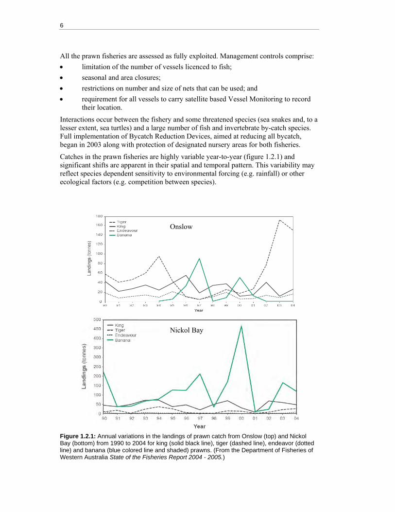
All the prawn fisheries are assessed as fully exploited. Management controls comprise: • limitation of the number of vessels licenced to fish; • seasonal and area closures; • restrictions on number and size of nets that can be used; and • requirement for all vessels to carry satellite based Vessel Monitoring to record
their location.
Interactions occur between the fishery and some threatened species (sea snakes and, to a lesser extent, sea turtles) and a large number of fish and invertebrate by-catch species. Full implementation of Bycatch Reduction Devices, aimed at reducing all bycatch, began in 2003 along with protection of designated nursery areas for both fisheries.
Catches in the prawn fisheries are highly variable year-to-year (figure 1.2.1) and significant shifts are apparent in their spatial and temporal pattern. This variability may reflect species dependent sensitivity to environmental forcing (e.g. rainfall) or other ecological factors (e.g. competition between species).
Figure 1.2.1: Annual variations in the landings of prawn catch from Onslow (top) and Nickol Bay (bottom) from 1990 to 2004 for king (solid black line), tiger (dashed line), endeavor (dotted line) and banana (blue colored line and shaded) prawns. (From the Department of Fisheries of Western Australia State of the Fisheries Report 2004 - 2005.)
Onslow
Nickol Bay

Introduction 7
Management of these highly variable target species within acceptable limits is a major challenge for any management strategy, particularly when combined with EBPC requirements to address ecological impacts of the fishery. Key recommendations made after the last EPBC assessment (DEH 2004) included requirements for monitoring and minimising protected species interactions, bycatch and other marine environmental impacts related to spawning areas, nursery grounds, feeding areas, and benthic habitats.
Oil and gas extraction Oil was first discovered in Western Australia at Rough Range in 1953 with exploration of crude oil and condensate beginning in 1962 and 1972 respectively. The industry has grown rapidly and by 2001 there were 44 fields producing in four sedimentary basins with the majority of these fields (32) contained within the Northern Carnarvon basin (figure 1.2.2). During 2001 these fields collectively produced 26 GmP
3P of gas and 20 Gl
of oil and condensate valued at 9.4 trillion dollars.
Woodside Energy and BHP Billiton Petroleum operations in the Pilbara region produced A$4.2 billion of crude oil, A$2.9 billion of LNG, A$1.7 billion of condensate, A$600 million of natural gas and over A$400 million of LPG products. The major oil and gas project in the Pilbara is the A$12 billion North West Shelf Joint Venture. The project is located on the Burrup Peninsula and currently has a production capacity of over 7.5 megatonnes per annum of LNG that is primarily exported to Japan. The North West Shelf Joint Venture project is equally owned by Woodside Energy; BP Developments Australia; Chevron Texaco Australia; BHP Billiton Petroleum; Shell Development (Australia); and Japan Australia LNG (MIMI).
Figure 1.2.2: Petroleum leases, all wells drilled including exploration and production, and major pipelines.

8
Coastal industries and development The major coastal industries in the study region are associated with oil and gas processing and distribution, salt production, and iron ore processing:
Oil and gas Woodside’s on-shore gas plant is located near Karratha and is Australia’s largest gas processing plant. The plant produces natural gas, liquid petroleum gas and condensate. A number of pipelines transport gas from the Pilbara to WA domestic markets (figure 1.2.2).
Mermaid Marine Australia Limited at Dampier is a major service facility for the oil and gas industry. The organisation operates a fleet of fifteen tugs, workboats and barges undertaking all forms of offshore activity including exploration support, supply, survey and berthing assistance.
Salt production The two salt producers on the North West Shelf are Dampier Salt Ltd and Onslow Salt Pty Ltd. Dampier Salt Ltd has two major operations located at Port Hedland and Dampier. In 2002, the Pilbara produced over six million tonnes of salt that represented 70 percent of the total salt produced in Western Australia for that year. The value of the Pilbara region’s salt production over this period was estimated to be A$180 million.
Iron ore Iron ore was discovered in the Pilbara region in the 1800s and the industry has now grown to include 22 iron ore mining and processing operations employing 9000 people. More than 95 percent of Australia’s iron ore exports are exported through the ports on the North West Shelf. In 2001, 157 million tonnes of iron ore worth A$5.1 billion was produced. The two major operators in the region are BHP Billiton Iron Ore and Rio Tinto (owner of Hamersley Iron and a majority holding in Robe River Iron Associates).
BHP Billiton Iron Ore has six mining operations in the Pilbara producing around 80 million wet tonnes of iron ore. The ore is railed to processing and shipping facilities at Port Hedland (where the Western Power electricity production facility generates a significant proportion of Western Australia’s electricity needs). Two port facilities located on opposite sides of Port Hedland harbour are connected by a 1.4 km under-harbour tunnel conveyor. Over 500 ships are loaded each year, the largest are up to 230 metres long and carry up to 260 000 tonnes of ore.
Hammersley Iron is located at Karratha and is one of the world’s leading iron ore producers, supplying 77 million tonnes of iron ore per year. Hamersley Iron uses gas to fire its 120-megawatt Dampier power station, which provides power to its mining facilities, port and processing operations at Dampier, the towns of Dampier, Tom Price and Paraburdoo, and the Dampier Salt facilities, with any surplus sold to Western Power's western Pilbara grid. Robe River operates two open pit mines in the Pilbara region, railing to a dedicated port at Cape Lambert from where over 40 million tonnes of iron ore are exported per year.

Introduction 9
1.3 Management strategy evaluation Management strategy evaluation (MSE) is a simulation based framework that can be used to test, compare and evaluate the outcomes of management strategies against defined performance measures that are derived from the objectives of management (e.g. Sainsbury et al. 2000; Sainsbury & Sumalia, 2003). A management strategy in this context is a combination of: • a monitoring program; • status assessments of indicators based on analyses of the monitoring data; • defined management responses that depend on the status assessments; and • implementation of the management measures.
MSE can be used to compare, in terms of the performance measures, strategies that differ in any of these aspects.
Because the MSE methodology compares management strategies using performance measures derived from management objectives, the comparisons are of overall management performance, rather than of performance of intermediate parts such as scientific accuracy of the monitoring program or the kind of management response. MSE treats the ecosystem, the human uses and the management system as a single coupled system, and evaluates the contribution of any part in terms of the overall outcomes rather than by performance of that part in isolation. This is because the outcome from the whole system is a function of the interacting parts. For example, an accurate monitoring program is unlikely to result in good overall outcomes if it delivers to an unresponsive management system, whereas good outcomes could be obtained from inaccurate monitoring that delivers into a suitably designed and responsive management system.
MSE explicitly includes uncertainty at all levels including: • the dynamics of the ecosystem or socio-economic system; • the effects of human use or activity; • the monitoring program; and • implementation of management measures.
Consequently it can examine the robustness of existing or proposed strategies to deliver management objectives despite recognised uncertainties. However, the conclusions about the robustness of a management strategy ultimately depend on adequate representation of uncertainty in the models that are used. While recognised uncertainties can be included in the MSE methodology, like other methodologies, it is vulnerable to uncertainties that are not yet recognised or recognisable.
Because it explicitly includes uncertainty, the MSE methodology can be used to estimate the gain in management performance from investments that resolve key uncertainties. In this context it is ideally suited to the development and testing of adaptive management strategies that make use of a ‘detection-correction’ feedback loop to robustly achieve desired outcomes despite uncertainty. This is typically in the form of monitoring and status assessments of indicators to detect departure from intent, with any necessary correction through planned management responses. Hence, MSE can be used to determine the monitoring, assessment and management response that will robustly lead to the desired management outcomes under the recognised uncertainties.
10
Management strategy evaluation for multiple uses One of the key objectives of NWSJEMS was to develop and demonstrate science-based methods and tools to support integrated regional planning and multiple-use management for ecologically sustainable development of the North West Shelf ecosystem, including management of the individual and cumulative effects of the various human uses and activities. While MSE has been applied previously to the management of individual industry sectors or activities, such as fisheries (Sainsbury et al. 2000), forestry (Sit & Taylor, 1998), water allocation (Walter et al. 2000), and insect pest control (Andow & Ives, 2002), it has not previously been applied to multiple human uses at the ecosystem level.
There are significant challenges in applying MSE to the multiple use management of the North West Shelf ecosystem. These stem from the high level of uncertainty about ecosystem processes and the complexity of representing the impacts, the benefits, the future development, and the interaction of management strategies of several industry sectors acting simultaneously. However, the fundamental approach is the same as for simpler applications and involves: • defining the management objectives, indicators and performance measures for
the industry sectors, the management agencies, and for the bioeconomics of the region as a whole;
• developing models to represent the range of ways the biophysical world may work;
• developing models to represent the activities, impacts and benefits from the industry sectors and other human uses, including expected future industrial developments; and
• developing models to represent possible monitoring and management strategies.
Together these models are designed to simulate environmental, social and economic conditions associated with the state of an ecosystem, as it evolves in response to natural forcing and human use (figure 1.3.1). Once they have been calibrated against available historical information and the model specifications have been defined, they can be used to compare the range of outcomes expected under potential future scenarios with alternative management strategies.
Model specifications A model specification is a description of the computer representation of the real system, including both the natural ecosystem and relevant components of human society. Uncertainty or inadequacy in process understanding usually leads to several alternative model specifications, all consistent with available system information, but varying in their structure and/or parametre values. These various specifications represent alternative hypotheses about how the system behaves in response to natural events and human actions and can include uncertainties about natural events (e.g. frequency and nature of catastrophic events) and human actions (e.g. motivations and behavioural rules).

Introduction 11
Development scenarios A development scenario is a statement of how various factors that impact on the system may change into the future. It is not included explicitly in the model specifications, but rather is used as input to the models. In the present context, development scenarios typically include demographic changes, industrial development, and climate change and variability.
Management strategies A management strategy is an existing or planned course of action employed, in the current context, by a government regulator or planner that constrains human use to achieve environmental, social or economic objectives. Along with these objectives, the management strategy must include a monitoring strategy that measures the state of the managed system through time and space and allows environmental, social and economic indicators to be calculated. Management responses are initiated and implemented based on the interpretation of these indicators relative to some target or performance measure.
MSE can also include industry-sector or business strategies aimed at achieving industry-wide or business outcomes. These have a similar structure to the management strategy of a regulator in that they contain objectives, monitoring and decisions in response to the monitoring information. Strategies at government, industry-sector or business level are all conducted within the context of relevant policy or governance arrangements. In the case of government regulators all or part of this may be provided through legislation.
MSE outputs For each combination of model specification, scenario and strategy, MSE provides output data in the form of data files, maps (e.g. GIS layers), and other graphical representations of the properties and indicator variables of interest. The display of these data may then be used to compare and contrast different combinations of model specification, scenario or strategy. Overlays of maps and images can be used to describe the spatial characteristics of the ecosystem at particular times. Such overlays can be updated through time to produce animated maps and images that show the dynamical evolution of the modelled system under the various combinations.

12
PERFORMANCEMEASURES
Natural forcesHuman impacts
PhysicsBio-geo-chemistryOil and gasConservation (habitat,fish, mega fauna)Coastal development
Observation model andmonitoring program (incl.performance indicators)
Perception ofbiophysical stateOil and gas regulationsConservation regulationsFishery regulationsCoastal developmentregulations
SECTORS
OIL AND GASObservation modelDecision process
CONSERVATIONObservation modelDecision process
FISHERYObservation modelDecision process
COASTALDEVELOPMENTObservation modelDecision process
BIOPHYSICAL MODEL
OBSERVATION AND MANAGEMENT MODEL
ENVIRONMENT AND MANAGEMENT
INPUTS OUTPUTS
INPUTS OUTPUTS
ASSESSMENT OFMANAGEMENT
STRATEGIES
Figure 1.3.1: The multiple-use MSE model framework. The components represented on the left side of the figure include both the biophysical ecosystem and the socioeconomic model of the region, as well as the management objectives and derived performance measures with which to judge the overall outcomes of the management strategy being evaluated. The socioeconomic model of the region generates performance measures that integrate across all activities and industries, as well as providing population and other inputs to the industry sector models. The right side of the figure contains the various human use sectors, including both their development and regulation. The human use sectors considered in NWSJEMS are oil and gas, fisheries, coastal development and conservation. For each industry sector, the sector models represent the activity of that industry, which provides both impacts in the biophysical model and costs/benefits to that industry sector. The assessment and monitoring models provide the information available through the monitoring and assessment program to inform industry or government for decision makers. For the oil and gas, coastal development and fisheries sectors there are separate industry and government observation programs. The management/policy/governance models make use of the information available through monitoring and assessment to reach decisions about change in industry activities or in government management measures. Industry and government decision making is made separately in the context of the relevant policy and governance arrangements. The tactical sector management model provides implementation of the decisions reached by the industry and by government regulators and included tactical responses by industry to changed regulation. The solid lines indicate the direct or primary effects of one component on another, while broken lines indicate indirect or secondary effects.

Introduction 13
1.4 Specification of multiple use management strategy evaluation for the North West Shelf region
MSE requires a computer representation of the natural ecosystem which influences, and is influenced by, human activity. This computer representation is made up of three components: • an ‘operating model’ of the biophysical and human systems involved, including
models of human impacts and the representation of uncertainty; • a range of scenarios for future social and industrial development in the region;
and • prospective management strategies (i.e. monitoring, assessment of monitoring
information, management response to the assessed information, and implementation of the management response).
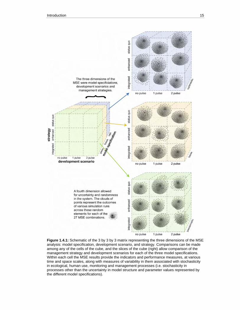
The MSE application to the North West Shelf region uses three different specifications of each of these three components, giving a 3 by 3 by 3 matrix of combinations through which to explore and compare sensitivities and outcomes. This matrix is made up of three operating model specifications, three development scenarios and three management strategies, giving 27 combinations for evaluation and comparison. This allows initial screening of behaviour that could be examined using a more complete or targeted MSE exploration of the options and outcomes (figure 1.4.1). In particular, it allows examination of the robustness of the different management strategies in delivering desired management outcomes for a range of possible future socio-economic development, despite uncertainty about how the ecosystem works. Although clearly a great simplification of the full range of interactions among these three dimensions, the 27 combinations chosen are sufficient to demonstrate the utility of MSE as a science-based aid to regional and sectoral planning and decision making.
Three model specifications were chosen that reflect: • an optimistic interpretation of the ecosystem’s productivity and resilience; • a central or base-case interpretation; and • a pessimistic interpretation.
These different model specifications reflect uncertainty about the dynamics of the ecosystem, both with respect to the structuring of the model and the values of the parameters in the model. Each model consists of sub-models of various processes or entities in the ecosystem that were individually modified to give the three models used in the MSE comparisons. So, for example, the optimistic operating model was optimistic in all of its submodel specifications.
Three development scenarios were chosen that represent: 1. the 2003 levels of infrastructure, residential and industrial development and
environmental protection, with no further development; 2. planned industrial development over the following five years (i.e. development
for the next five years that is presently under construction or at an advanced stage of planning or approval) with no further development from 2008; and
3. as in (2) to 2008, followed by similar development over the following 5 years, with no further development from 2013.

14
Each development scenario contains an individual development plan for each of the four industry sectors considered (i.e. oil and gas, coastal development, fishing, and conservation) according to the development planned for that sector in the five years from December 2002.
The three development scenarios can be regarded as examining the consequences of no further development, one 5-year pulse of additional development, and two 5-year pulses of further development. The first development scenario allows examination of the long-term outcomes of the present level of development, recognising that many relevant environmental and economic outcomes are relatively slow to fully manifest and that all outcomes of the present level of development may not yet be observable in the real world. Similarly, the second development scenario examines the short and long-term consequences of the development planned in the next five years. The third scenario considers the consequences of sustaining this development over 10 years.
Three management strategies were chosen to reflect different possible approaches to government management and regulation: • status quo management arrangements taken to be the sectorally based
management strategies in place at the start of 2003; • enhanced status quo management arrangements, which maintained the form of
the current sectorally based management strategies but increased the monitoring, assessment and implementation with the intention of reflecting the best outcomes likely to be achieved by this structure of management; and
• enhanced regional management arrangements, which set regional indicators and benchmarks, coordinated monitoring, shared the results of monitoring and assessment among sectors, and provided a multi-sectoral management response if undesirable trends were detected in monitored indicators.
The MSE calculations and comparisons were conducted to represent the 12 year period January 2003 to December 2014. Within each cell of the 3 by 3 by 3 matrix (figure 1.4.1) several hundred indicators were calculated and provided at several time and space scales (section 4.6). For relevant indicators statistical measures of variability are also provided that reflect stochasticity in ecological, human use, monitoring and management processes (i.e.stochasticity in processes other than the uncertainty in model structure and parameter values represented by the different model specifications). Two computer visualisation packages are provided to allow examination of these indicators; one tailored for scientific exploration, diagnosis and statistical analysis, and the other for more general visualisation and inspection (Hatfield et al. 2006).
Introduction 15
Figure 1.4.1: Schematic of the 3 by 3 by 3 matrix representing the three dimensions of the MSE analysis: model specification, development scenario, and strategy. Comparisons can be made among any of the cells of the cube, and the slices of the cube (right) allow comparison of the management strategy and development scenarios for each of the three model specifications. Within each cell the MSE results provide the indicators and performance measures, at various time and space scales, along with measures of variability in them associated with stochasticity in ecological, human use, monitoring and management processes (i.e. stochasticity in processes other than the uncertainty in model structure and parameter values represented by the different model specifications).

16
2. MODEL SPECIFICATIONS
The models used for the MSE calculations are described in detail in Gray et al. 2006 and are comprised of a combination of agent-based sub-models and the more usual equation based sub-models. The agent-based models are comprised of agents, objects or entities that behave autonomously. These agents are aware of, or interact with, one another and their local environment through simple internal rules for decision making, movement, action or reaction. Aggregate behaviour is the result of a large number of these interactions, and can be complex even if the interaction rules are simple. Agent-based modelling has been successfully applied to predict movement of gas or fluid particles, population and ecological properties from individual animal interactions, business selections in financial markets, and human responses on battlefields. Agent-based models are particularly appropriate where complex behaviour is thought to arise from discrete interactions or decisions by heterogeneous entities, such as movement of animals or economic decision making of humans. Agent-based models are easily modified, can represent complex system behaviour and situations that are not well summarised by average or ‘mean field’ descriptions. However, because they are more computationally intensive than equation-based models, the MSE model uses equation-based sub-models where the unit of interest represents a large number of individuals and so the particular benefits of agent-based sub-models are not evident (e.g. entire populations or habitat patches that are many kilometres in scale).
The two main aspects of specification for MSE models are the model structure and the model parameters for a given model structure. Several different structures were examined for the sub-models of the main biophysical processes and human impacts, including alternative equation-based and agent-based variations for many sub-models. Combinations of model structure and parameter values were examined that could reasonably match any available historical data. Goodness of fit to historical data was measured by the sum of squared differences between the observations and model predictions. Model parameters corresponding approximately to the least squares estimates and the 80% confidence intervals were used to identify a reasonable span of possible parameter values and sub-model behaviours.
From the range of sub-model structure and parameter combinations that satisfied the above criteria, an ‘optimistic’ set was chosen corresponding to relatively high levels of system productivity and resilience to human impacts (i.e. relatively productive fish resources, fast recovery of habitat after disturbance, and low uptake or fast elimination of contaminants by organisms). A ‘pessimistic’ set was similarly chosen corresponding to relatively low levels of system productivity and resilience to human impacts (i.e. relatively unproductive fish resources, slow habitat recovery after disturbance, and high uptake or slow elimination of contaminants by organisms). The sub-models for the ‘base-case’ interpretation used the least squares parameter estimates, where these could be reasonably calculated, or otherwise the most reasonable estimates available from studies reported in the scientific literature.
In the remainder of this chapter details on each of the main sub-models of the operating model will be provided, including more detailed definition of the optimistic, base-case and pessimistic interpretations. The main sub-models included: • Water circulation and particle transport

Model specifications 17
• Primary production and nutrient cycling • Benthic habitat • Iconic species dynamics • Fish species and impacts of fishing • Dispersal and uptake of contaminants • Human behaviour and impact
Parameter values corresponding to the optimistic, base-case and pessimistic interpretations are listed in Appendix E.
2.1 Water circulation and particle transport The model used to compute the currents on the North West Shelf was based on MECO (Model for Estuaries and Coastal Oceans) modelling system, which is documented in Herzfeld et al. (2002). MECO is a general-purpose finite difference hydrodynamic model applicable to scales ranging from estuaries to ocean basins. It has been applied previously to systems such as the Derwent and Huon estuaries in Tasmania, Gippsland Lakes, Port Phillip Bay (Walker, 1999), Bass Strait, the Great Australian Bight and South-eastern Australia (Bruce et al. 2001), and the Gulf of Carpentaria (Condie et al. 1999). A full description of the circulation model as applied to North West Shelf and descriptions of the spatial and temporal characteristics of the circulation and connectivity can be found in Condie et al. (2006).
The model produced data on three nested grids, designed to capture the dynamics over a range of spatial scales. Each of these was a rotated latitude-longitude grid and could be described as follows: • A large regional model with horizontal resolution of approximately 10 km,
extending from Cape Cuvier (south of Coral Bay) to the Bonaparte Archipelago and well beyond the shelf break. This was referred to as the Northwest model.
• A smaller regional model with horizontal resolution of approximately 5 km, extending from Ningaloo to Port Hedland and beyond the shelf break. This was referred to as the Pilbara model.
• A localised coastal model with horizontal resolution of approximately 1 km, covering the waters around the Dampier Archipelago to depths of almost 50 m. This was referred to as the Dampier model.
The circulation and particle transport data produced by these three nested models is very comprehensive and was assumed to be the best description of water circulation and particle transport available for the NWS. However, the run times of these models were much too long to be imbedded directly into MSE model and still allow the multiple runs needed to adequately represent stochasticity. It was not even practical to store the fully detailed circulation model outputs and use them to construct the necessary input to the MSE models. Instead a much simpler statistical model was calibrated against the circulation model outputs and then used to predict the short-term circulation and particle transport within the MSE model. This statistical model was mainly used in the MSE to predict contaminant dispersion and is described in this context in section 2.6.

18
2.2 Primary production, nutrient cycling and trophic interactions
Detailed models of the primary production, nutrient cycling and trophic interactions have been developed for the North West Shelf (Herzfeld et al. 2006; Bulman, 2006). While agent-based models where also developed incorporating such interactions, they were found to be too slow for deployment at regional scales. Furthermore, the results of Herzfeld et al. (2006) and Bulman (2006) suggest that there is limited interaction of these processes with the human uses examined by the MSE. Instead, the major effects of the human uses were through the more direct consequences of harvesting, habitat modification and water quality. With respect to fisheries this is consistent with the findings of Sainsbury (1988). It was therefore decided not to explicitly represent processes such as primary production (beyond the growth of habitat forming primary producers such as macroalage, mangroves and seagrass, which were included for their habitat role), nutrient cycling and trophic interactions in the current application of the MSE model.
2.3 Benthic habitats The benthic habitats represented in the MSE included coastal habitats, such as seagrass meadows and mangrove forests, and continental shelf habitats, differentiated by sediment type and coverage of epibenthic fauna such as sponges and soft corals.
A number of statistical and analytical models of the benthic habitats were developed (Fulton et al. 2006) and used to guide both the structure and parameter values used in the operating model. These were most fully developed for the continental shelf seabed habitats because of the availability of relevant historical data. Given these data and the nature of the underlying processes, a metapopulation model was developed to calculate percentage cover, height and biomass of benthic fauna through time. This approach was adapted from previous habitat and metapopulation modelling work (e.g. Levins, 1969; Sainsbury 1991; Tilman & Kareiva, 1997). The benthic habitat models used sediment properties as a contributing factor to the benthic habitat distribution (Jones, 1973; McLoughlin & Young, 1985; Colman & West, 2000; figure 2.3.1).
Parameter values were derived from local habitat data and information from the broader scientific literature. There was relatively little documentation available on historical habitat distributions, which was mostly obtained through structured interviews and workshops with residents, divers and scientists with long-term experience on the NWS. Parameter options were calibrated to be consistent with the available data on each habitat type, as well as the range of views about the historical distributions.
Each of the habitat types was modelled using the ‘benthic agent’ model structure (Gray et al. 2006), which allowed for horizontal and vertical growth of habitat patches, ageing, mortality, fragmentation due to external events (e.g. cyclones, dredging), and either constant or density dependent colonisation of new habitat patches.

Model specifications 19
Key
100
0
(a) gravel
(b) sand
(c) silt
(d) clay
Figure 2.3.1: Sediment composition map. The index (colour key) is a percentage composition of the sediment for the grain type (gravel, sand and silt); similarly for the percentage composition of lay except the scale is 0 to 10 not 0 to 100.
Each agent was represented by a series of habitat polygons covering specified areas with resolutions considered appropriate for the habitat type. For the continental shelf reef habitats, the polygons consisted of a regular grid (six minutes of latitude by six minutes of longitude). The seagrass and macroalgae grids were on a larger grid (12 minute by 12 minute) but restricted to depths of less than 50 m. The mangrove grids were on a finer grid (three minute by three minute) and restricted to the coastline. While these grid sizes were fixed, sub-grid scale fragmentation and and patchiness were modelled in combination with the percentage cover of the various habitat types.
20
Two formulations of the benthic agent model were used: 1. Coastal mangroves and shelf reef habitats (mainly sponges and soft corals) were
represented by an age-structured model, with percentage cover of small and large organisms tracked separately. Small and large were defined as < 100 cm and > 100 cm for mangroves and as < 25 cm and > 25 cm for sponges and soft corals. For any habitat type, patches of these two different size classes may overlap, so while the percent cover of either small or large habitat categories separately is ≤ 100%, the sum of the percent cover of small and large categories is ≤ 200%.
2. Seagrass and macroalgae were represented by a model with light limitation, but no age-structuring.
For each habitat agent the percentage cover, average height and biomass is tracked for each polygon. These statistics were used individually as indicators of the extent and character of each habitat, and in combination as proxies for biodiversity. Empirical observations suggest that there is a direct relationship between biodiversity and the average height of organisms in biogenic habitats such as sponge beds (Keith Sainsbury, Franzis Althaus and Piers Dunstan pers. comm. CSIRO Marine and Atmospheric Research).
Parameter estimation For continental shelf reef habitat the base-case parameters for the habitat equations were determined by least squares optimisation. The Simplex method of minimising the sum of squares was used to fit the model to the benthos observations, with some parameters further constrained to a biologically meaningful range (Fulton et al. 2006). For the seagrass, macroalgae and mangrove habitats there was very limited documented information available from which to estimate model parameters. For these habitats the base-case parameters were determined from expert information and heuristic fitting to available data on historical cover and distributions (Lyne et al. 2006). The base-case parameter sets for each of the habitat types are given in Appendix B.
The pessimistic and optimistic parameterisations were determined by considering the extremes of the relevant parameters in the literature and by exploring the dynamics of the system in the parameter space around the base case results. The pessimistic parameters were selected so that the impact of disturbances on the habitat groups was stronger than in the base case and the rates of recovery were slower. Conversely, in the optimistic specification, the parameters were selected so that impacts were smaller and the rates of recovery faster. However, the parameter selection was constrained such that the resulting habitat cover predictions were plausible given the available data sets and expert opinions on historical habitat cover. Where statistical methods could be applied, the 80% confidence interval was used to identify the optimistic and pessimistic bounds. The optimistic and pessimistic bounds were much wider for the seagrass, macroaglae and mangrove habitats than for the continental shelf habitats, because of the different quantity and quality of the information available.
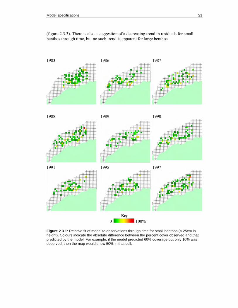
The model of the continental shelf habitats provides a relatively good description of the available observations for both small reef habitat (figure 2.3.2) and large reef habitat (figure 2.3.3). The temporally-pooled residuals between prediction and observation are generally low, although there are some exceptions in the case of small reef habitat
Model specifications 21
(figure 2.3.3). There is also a suggestion of a decreasing trend in residuals for small benthos through time, but no such trend is apparent for large benthos.
1983
1986
1987
1988 1989 1990
1991 1995 1997
Key 0 100%
UFigure 2.3.1: Relative fit of model to observations through time for small benthos (< 25cm in height). Colours indicate the absolute difference between the percent cover observed and that predicted by the model. For example, if the model predicted 60% coverage but only 10% was observed, then the map would show 50% in that cell.

22
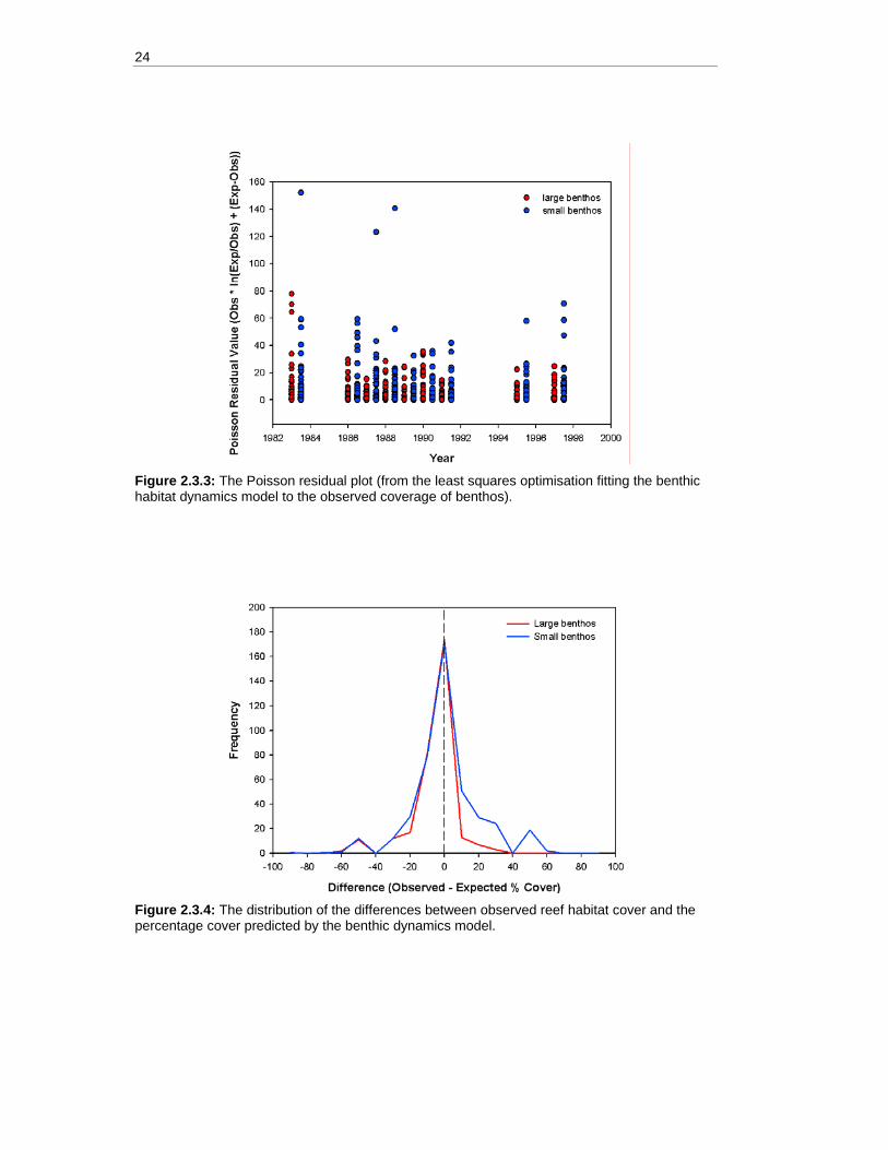
When considering the percentage cover per grid cell predicted by the model, 84% of the predictions for large reef habitat and 70% for small reef habitat fall within the credibility bands of observed values. While the tails of these distributions fall away quickly (figure 2.3.4) there was at least one prediction that differed from the observation by as much as 90%. There is a tendency for the model to underestimate the cover of large reef habitat (i.e. the curve in figure 2.3.4 is shifted to the left) which is not evident for small habitat. These mismatches are mostly due to sub-grid scale patches of reef habitat that are not well resolved by the model. Nevertheless the model generally provides a good representation of overall distributions and general levels of cover.
There were insufficient data to repeat the quantitative fitting process and model testing for the seagrasses, macroalgae and mangroves. In the MSE context this necessitated large differences in the optimistic and pessimistic specifications so as to encompass the underlying uncertainties. While a small amount of data was available on the species present and their overall geographic range (Walker & Prince, 1987; Semeniuk, 1994; Semeniuk & Semeniuk, 1995; Carr & Livesey, 1996; Semeniuk & Semeniuk, 1997; Bridgewater & Cresswell, 1999; Australian State of the Environment Committee 2001; Prince, 2001), the required fine-scale information on the spatial distributions, presence-absence and depletion-recovery rates was mainly obtained through expert information (McCook et al. 1995; Paling, 1996; McGuinness, 1997; Moran & Stephenson, 2000; Kathiresan & Bingham, 2001; Lyne et al. 2006). As a result the parameters for these habitat forming groups were calibrated via a sensitivity analysis to give the best match to available data.

Model specifications 23
1983 1986 1987
1988 1989 1990
1991 1995 1997
Key 0 100%
Figure 2.3.2: Relative fit of model to observations through time for large benthos (> 25cm in height). Colours indicate the absolute difference between the percent cover observed and that predicted by the model.
The model fitting and sensitivity analyses indicate that the model is most sensitive to the mortality rate and vulnerability parameters. The values of these parameters are often quite small so minor differences in value represent substantial changes in relative rates. These small variations in mortality rates and vulnerability were used to discriminate between the optimistic, base, and pessimistic model specifications. In particular, the growth rate and trawl damage rate of reef habitat were varied between model specifications. The exact values used were selected on the basis of the net effect on model output, but all were drawn from the range of credible values given by the parameter fitting and all were well within the range found in the scientific literature.
24
Figure 2.3.3: The Poisson residual plot (from the least squares optimisation fitting the benthic habitat dynamics model to the observed coverage of benthos).
Figure 2.3.4: The distribution of the differences between observed reef habitat cover and the percentage cover predicted by the benthic dynamics model.

Model specifications 25
2.4 Iconic species The iconic species examined in the MSE are turtles and sharks. For both groups the populations were represented by the ‘animal agent’ model for post-larval stages and the ‘blastula agent’ for reproduction and spatial dynamics of very early life history stages (Gray et al. 2006). This representation supported density-dependent processes that can apply to natural mortality at egg, larval and post-larval stages. It also allowed for spatially explicit treatment of all pre-adult stages, which were confined to suitable habitats. Model sensitivity to this representation was evaluated by also implementing a more classical population model representation. Biological parameters for these species were taken from the literature (Limpus et al. 1984; Limpus & Reed, 1985; Kailola et al. 1993; Limpus et al. 1994; Last & Stevens, 1994; Chaloupka & Musick, 1997; Environment Australia 2000; Chaloupka, 2002; Chaloupka, 2003; Stephenson & Chidlow, 2003; Fishbase 2005) and modified slightly during model calibration to give plausible biomass levels under observed levels of fishing pressure and catch.
There was a domestic fishery directed at turtles on the North West Shelf from around 1958 to 1973, in which about 60 000 turtles were taken including 5,000 to 6 000 per annum in the later years of the fishery (pers. comm. 2005 from Bob Prince, CALM, and Kellie Pendoley and Liz McLellan, Asia Pacific Marine Turtle Programme WWF International). More recent fishery catches of turtles have been as incidental bycatch. Between 1999 and 2002 a reporting program involving five of the 45 prawn fishing vessels in Onslow and Nickol Bay recorded a total of 22 turtles (all adults) implying an annual bycatch of approximately 66 adult turtles. Bycatch exclusion devices began being used in the fishery in 2003, and there have been no reported turtle captures since.
As for the other ecological model components, parameterisation for the pessimistic and optimistic model specifications were selected by considering the extremes of the literature values and by exploring the dynamics of the model system in the parameter space around the base case. Parameter sets were then chosen to give relatively low vulnerability and/or fast recovery for the optimistic case and vice versa for the pessimistic case, while still giving plausible historical trajectories of total biomass and catch. This process was particularly problematic for turtles, which suffer from undocumented mortality such as catch beyond the Australian jurisdiction, injuries as they pass through nets (Limpus et al. 1984), vessel strikes, egg collecting and other disruptions to nests or nesting. While inclusion of three models helps to span such contingencies, the recovery dynamics are sensitive to the model structure even after tuning to the same data and literature parameters (Little et al. 2006) and there remains a significant risk that turtle recovery rates were overestimated even in the pessimistic model.
Initial biomasses The initial turtle biomass estimates where primarily based on information relating to Chelonia mydas (Green), but also included available data on Lepidochelys olivacea (Olive Ridley), Caretta caretta (Loggerhead), Eretmochelys imbricata (Hawskbill), Natator depressus (Flatback) and Dermochelys coriacea (Leatherback). The primary data sources were:
26
• Australia-wide stock estimates given in the 1995 Status of the Marine Environment Report (Zann 1995) and the Australian State of the Environment Report 2001 (Australian State of the Environment Committee, 2001);
• values estimated from the 1997 survey of the Gulf of Carpentaria (Marsh et al. 2004);
• the 1985 survey of the northern Great Barrier Reef Marine Park (Marsh & Saalfield 1989);
• values given for other northern Australian sites (Limpus et al. 1984; Limpus & Reed 1985; Limpus et al. 1994; Chaloupka 2002; Chaloupka 2003); and
• expert information (pers. comm. Bob Prince, Leader of the Western Australian Marine Turtle Project CALM; Kellie Pendoley, Western Australian turtle researcher; and Liz McLellan, Asia Pacific Marine Turtle Programme, WWF International).
The expert information provided important information on a poorly documented commercial turtle fishery that was active in the Pilbara area in the early 1970s and likely to have had substantial impacts on populations. Together these data sources lead to a final estimate for the turtle abundance of between 18 000 and 45 000 individuals (assuming an average adult weight of 50 kg).
The initial biomass of sharks on the North West Shelf was calculated using the value given for coastal sharks in the Ecopath model developed for the North West Shelf (Bulman 2006). Using the Ecopath model value of 0.03 tonnes per kmP
2P, a total
abundance of between 10 000 and 28 000 individuals was derived. This equates to an average total biomass of roughly 1260 t (assuming an average adult shark is between 45 and 125 kg in weight).
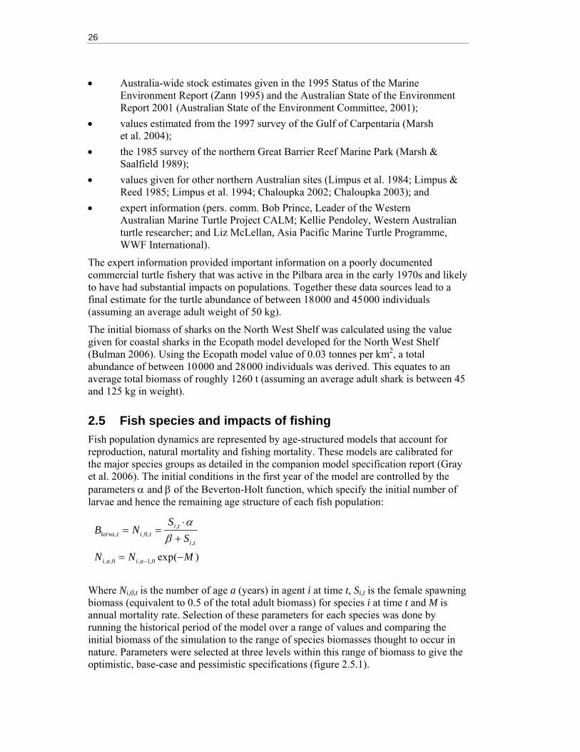
2.5 Fish species and impacts of fishing Fish population dynamics are represented by age-structured models that account for reproduction, natural mortality and fishing mortality. These models are calibrated for the major species groups as detailed in the companion model specification report (Gray et al. 2006). The initial conditions in the first year of the model are controlled by the parameters α and β of the Beverton-Holt function, which specify the initial number of larvae and hence the remaining age structure of each fish population:
Where Ni,0,t is the number of age a (years) in agent i at time t, SBi,tB is the female spawning biomass (equivalent to 0.5 of the total adult biomass) for species i at time t and M is annual mortality rate. Selection of these parameters for each species was done by running the historical period of the model over a range of values and comparing the initial biomass of the simulation to the range of species biomasses thought to occur in nature. Parameters were selected at three levels within this range of biomass to give the optimistic, base-case and pessimistic specifications (figure 2.5.1).
,, ,0,
,
i tlarva t i t
i t
SB N
Sα
β⋅
= =+
, ,0 , 1,0 exp( )i a i aN N M−= −
Model specifications 27
Lutjanus sebae
0.05.0e+4
1.0e+51.5e+5
2.0e+5
2.5e+5
1000
10000
1000
10000
B0 (t
onne
s)
α
β
Large lutjanids (L. erythropterus, L. malabaricus)
05e+4
1e+52e+5
2e+53e+5
3e+5
1e+4
1e+5
100
1000
B0 (t
onne
s)
α
β
Lethrinids
02e+54e+56e+58e+51e+61e+61e+62e+6
2e+6
2e+6
1e+6
1e+4
1e+5
B0
(tonn
es)
α
β
Small lutjanids (L. vitta)
02e+5
4e+5
6e+5
8e+5
1e+5
1e+6
100
1000
B0 (t
onne
s)
α
β
Nemipterids
0.02.0e+54.0e+5
6.0e+58.0e+5
1.0e+61.2e+6
1.4e+61.6e+6
1.8e+6
1e+5
1e+6
1e+4
1e+5
B0 (t
onne
s)
α
β
Saurids
0.02.0e+54.0e+5
6.0e+58.0e+5
1.0e+61.2e+6
1.4e+61.6e+6
1.8e+6
1e+4
1e+5
1e+4
1e+5
B0 (t
onne
s)
α
β
Figure 2.5.1: Initial available species or group biomasses for different values of α and β (grey), and the maximum (orange) and minimum (yellow) biomass estimated to be in the system based on Bulman (2006). The intersection (red) represents parameter combinations that fall within the range.

28
Prawn biomass estimates The initial conditions and carrying capacity estimates for the prawn stocks were calculated using catch data and biological information taken from the WA Department of Fisheries (2002) submission to Environment Australia regarding the Exmouth Gulf Prawn Fishery. This information was converted to total stock sizes using the assessment rule-of-thumb that catch at Maximum Sustainable Yield equals 12% of virgin biomass and cross checked using the methods outlined in Taylor and Dichmont (2001). This resulted in an upper bound on the estimate of maximum total biomass of 15 000 tonnes for western king prawns, with a lower bound of 8 000 tonnes and a median of 12 000 tonnes. For banana prawns the upper bound on biomass was again 15 000 tonnes, while the lower bound was 4 000 tonnes and the median was 8 000 tonnes. All other prawn biological parameters were based on Kailola et al. (1993) and Taylor and Dichmont (2001).
2.6 Contaminants The MSE models included interactions of industrial contaminant plumes with local fauna. The specific sub-models used in simulating these interactions are described in Gray et al. (2006) along with strategies for developing more sophisticated models incorporating sublethal effects.
There are two fundamental aspects to modelling the interaction of contaminants with marine organisms, namely the way they come into contact with each other and what happens to them when they do. Direct contact with a contaminant occurs when the contaminant is suspended or dissolved in the water column, while indirect contact may occur through consuming organisms which have already come into contact. The MSE focused on simulating mortality due to direct contact, where the contaminant is ingested or taken in through the animal’s respiratory system. Allowance was also made for exposure to multiple contaminants.
Plumes were represented as relative concentration fields, decaying from unit value at the source to a low threshold (0.0001 units) at the furthest contour. These fields were then converted to a set of concentrate ions for each of the the contaminants associated with the source by multiplying by the reputed source concentration and a factor that can account for uncertainty or misreporting of concentrations. This approach allows contours calculated for a unit source to be used for all contaminant types and concentrations from that source. It also provides a convenient framework in which to model management strategies that adaptively adjust contaminant inputs in response to monitoring of the system.
Data on the effects of particular contaminants on particular organisms are very limited, particularly with regard to sublethal effects on behaviour or reproductive capacity. The modelling was therefore focused on lethal impacts through either acute exposure or chronic exposure leading to more gradual accumulation in the tissue until a lethal level was reached. Uptake rates were specified for each impacted species by using the model to replicate outcomes of a study by Hashmi et al. (2002), in which heavy metal concentrations in tiger prawn tissue samples and their water environment were taken from two prawn farms subject to different contaminant loads. The optimistic, base-case and pessimistic interpretations were defined in terms of the exposure levels as determined by the the contaminant plume dynamics and the distribution of impacted organisms.
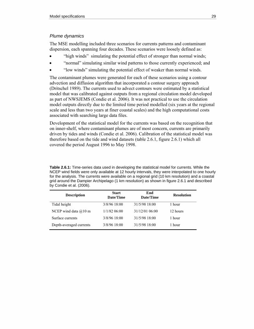
Model specifications 29
Plume dynamics The MSE modelling included three scenarios for currents patterns and contaminant dispersion, each spanning four decades. These scenarios were loosely defined as: • “high winds” simulating the potential effect of stronger than normal winds; • “normal” simulating similar wind patterns to those currently experienced; and • “low winds” simulating the potential effect of weaker than normal winds.
The contaminant plumes were generated for each of these scenarios using a contour advection and diffusion algorithm that incorporated a contour surgery approach (Dritschel 1989). The currents used to advect contours were estimated by a statistical model that was calibrated against outputs from a regional circulation model developed as part of NWSJEMS (Condie et al. 2006). It was not practical to use the circulation model outputs directly due to the limited time period modelled (six years at the regional scale and less than two years at finer coastal scales) and the high computational costs associated with searching large data files.
Development of the statistical model for the currents was based on the recognition that on inner-shelf, where contaminant plumes are of most concern, currents are primarily driven by tides and winds (Condie et al. 2006). Calibration of the statistical model was therefore based on the tide and wind datasets (table 2.6.1, figure 2.6.1) which all covered the period August 1996 to May 1998.
Table 2.6.1: Time-series data used in developing the statistical model for currents. While the NCEP wind fields were only available at 12 hourly intervals, they were interpolated to one hourly for the analysis. The currents were available on a regional grid (10 km resolution) and a coastal grid around the Dampier Archipelago (1 km resolution) as shown in figure 2.6.1 and described by Condie et al. (2006).
Description Start Date/Time
End Date/Time Resolution
Tidal height 3/8/96 18:00 31/5/98 18:00 1 hour
NCEP wind data @10 m 1/1/82 06:00 31/12/01 06:00 12 hours
Surface currents 3/8/96 18:00 31/5/98 18:00 1 hour
Depth-averaged currents 3/8/96 18:00 31/5/98 18:00 1 hour

30
Figure 2.6.1: Example time-series of data used to calibrate the statistical model: tidal height (top), eastward wind component (centre) and northward wind component (bottom). Time is in hours since 18:00 on 3 August 1996.

Model specifications 31
A number of alternate statistical models were considered including linked spatio-temporal models. The over-riding requirements for speed, efficiency and accuracy were satisfied by fitting low-order polynomial models for the currents at each station. While this approach required all currents to be calculated during run-time from stored polynomial coefficients, the storage and computation costs were very small compared to alternative approaches.
The statistical model used was a generalised linear model of third-order polynomials in tide, lagged-tide and NCEP winds. This was calibrated against the eastward and northward components of both the surface and depth-averaged currents derived from the circulation models (using the higher resolution Dampier Archipelago model when inside that domain – figure 2.6.2). The influence of spring-neap cycles and seasonal factors affecting wind and current regimes were considered, but preliminary analyses (e.g. additive and multiplicative models in spring-neap amplitude and phase) did not provide improved predictions. Inclusion of the lagged tide time-series (lagged by one time step) provided an indication of the phase of the tide (rising or falling) and substantially improved the predictions of the model.
Examples of the statistical fits are provided in table 2.6.2 and figure 2.6.3. These results indicate that the fit deteriorates offshore as the influence of regional currents (not accounted for in the model) increases. Nonetheless, 60 to 80% of the variance is explained near the coast for the example stations used. Example of the statistical parameters for one site are listed in table 2.6.3. On completion of the statistical fits, a database of station locations and the polynomial coefficients were incorporated into the InVitro system. These fits allowed efficient simulations of currents over any period that tide and wind data were available.
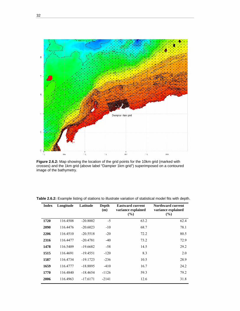
32
Figure 2.6.2: Map showing the location of the grid points for the 10km grid (marked with crosses) and the 1km grid (above label “Dampier 1km grid”) superimposed on a contoured image of the bathymetry.
Table 2.6.2: Example listing of stations to illustrate variation of statistical model fits with depth.
Index Longitude Latitude Depth (m)
Eastward current variance explained
(%)
Northward current variance explained
(%)
1720 116.4508 -20.8002 -5 63.2 62.4
2090 116.4476 -20.6023 -10 68.7 78.1
2206 116.4510 -20.5518 -20 72.2 80.5
2316 116.4477 -20.4781 -40 73.2 72.9
1478 116.5409 -19.6682 -58 14.5 29.2
1515 116.4691 -19.4551 -120 8.3 2.0
1587 116.4734 -19.1723 -236 10.5 28.9
1659 116.4777 -18.8895 -410 16.7 24.2
1770 116.4840 -18.4654 -1126 59.3 79.2
2006 116.4963 -17.6171 -2141 12.6 31.8

Model specifications 33
Figure 2.6.3: Example scatter plots for eastward (U) and northward (V) currents for to a shallow water station (upper, index 2090) and deep water station (lower, index 2006).
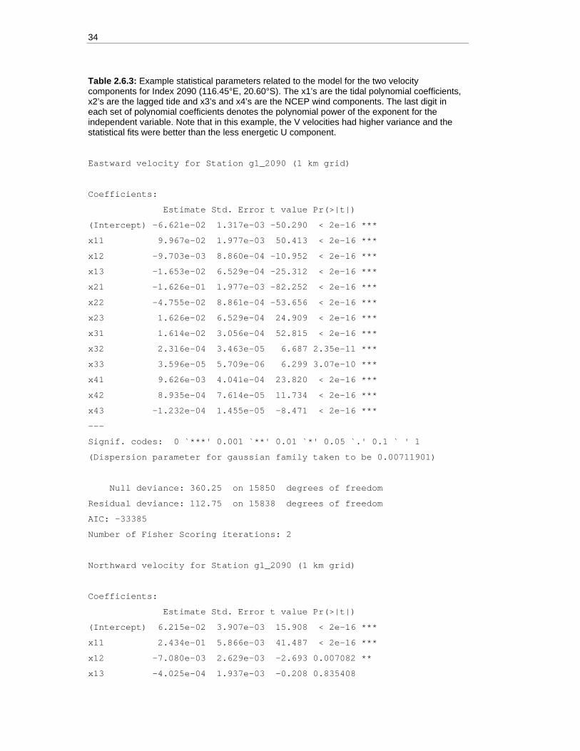
34
Table 2.6.3: Example statistical parameters related to the model for the two velocity components for Index 2090 (116.45°E, 20.60°S). The x1’s are the tidal polynomial coefficients, x2’s are the lagged tide and x3’s and x4’s are the NCEP wind components. The last digit in each set of polynomial coefficients denotes the polynomial power of the exponent for the independent variable. Note that in this example, the V velocities had higher variance and the statistical fits were better than the less energetic U component.
Eastward velocity for Station g1_2090 (1 km grid)
Coefficients:
Estimate Std. Error t value Pr(>|t|)
(Intercept) -6.621e-02 1.317e-03 -50.290 < 2e-16 ***
x11 9.967e-02 1.977e-03 50.413 < 2e-16 ***
x12 -9.703e-03 8.860e-04 -10.952 < 2e-16 ***
x13 -1.653e-02 6.529e-04 -25.312 < 2e-16 ***
x21 -1.626e-01 1.977e-03 -82.252 < 2e-16 ***
x22 -4.755e-02 8.861e-04 -53.656 < 2e-16 ***
x23 1.626e-02 6.529e-04 24.909 < 2e-16 ***
x31 1.614e-02 3.056e-04 52.815 < 2e-16 ***
x32 2.316e-04 3.463e-05 6.687 2.35e-11 ***
x33 3.596e-05 5.709e-06 6.299 3.07e-10 ***
x41 9.626e-03 4.041e-04 23.820 < 2e-16 ***
x42 8.935e-04 7.614e-05 11.734 < 2e-16 ***
x43 -1.232e-04 1.455e-05 -8.471 < 2e-16 ***
---
Signif. codes: 0 `***' 0.001 `**' 0.01 `*' 0.05 `.' 0.1 ` ' 1
(Dispersion parameter for gaussian family taken to be 0.00711901)
Null deviance: 360.25 on 15850 degrees of freedom
Residual deviance: 112.75 on 15838 degrees of freedom
AIC: -33385
Number of Fisher Scoring iterations: 2
Northward velocity for Station g1_2090 (1 km grid)
Coefficients:
Estimate Std. Error t value Pr(>|t|)
(Intercept) 6.215e-02 3.907e-03 15.908 < 2e-16 ***
x11 2.434e-01 5.866e-03 41.487 < 2e-16 ***
x12 -7.080e-03 2.629e-03 -2.693 0.007082 **
x13 -4.025e-04 1.937e-03 -0.208 0.835408
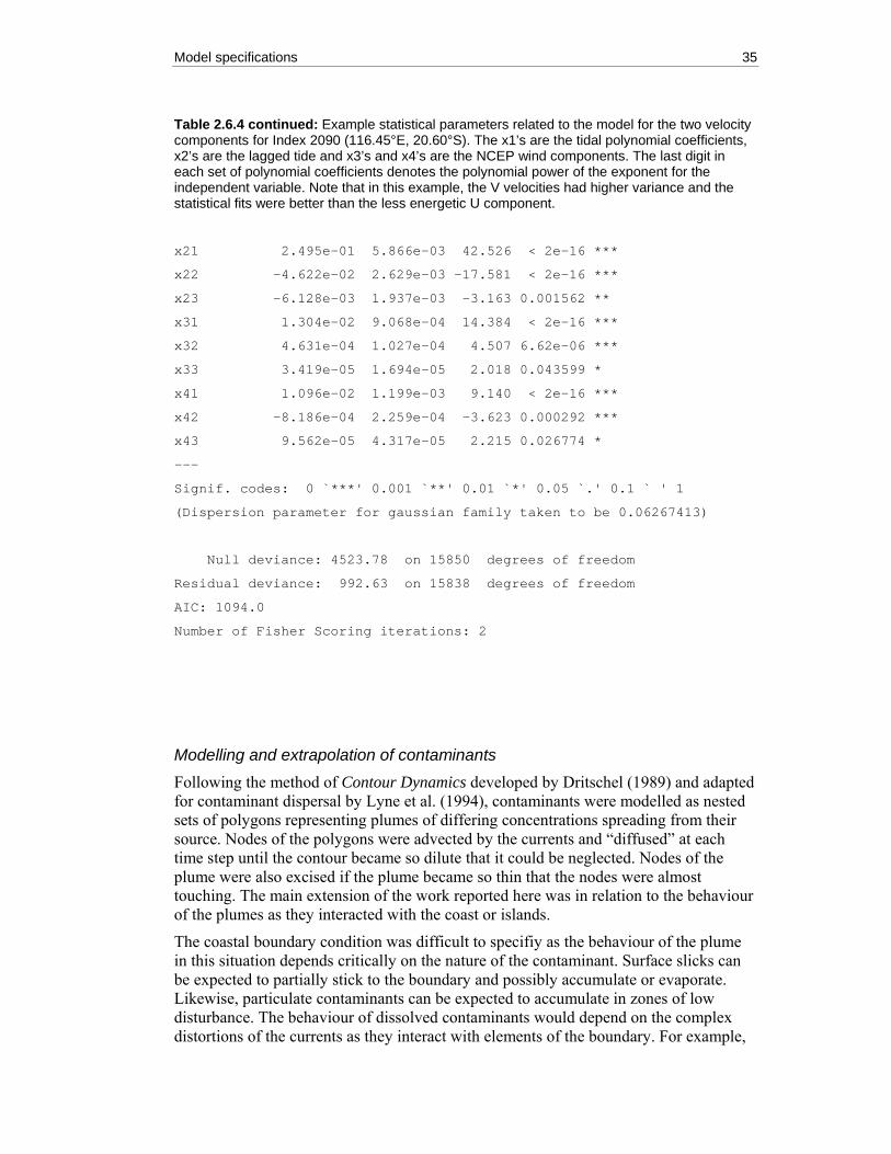
Model specifications 35
Table 2.6.4 continued: Example statistical parameters related to the model for the two velocity components for Index 2090 (116.45°E, 20.60°S). The x1’s are the tidal polynomial coefficients, x2’s are the lagged tide and x3’s and x4’s are the NCEP wind components. The last digit in each set of polynomial coefficients denotes the polynomial power of the exponent for the independent variable. Note that in this example, the V velocities had higher variance and the statistical fits were better than the less energetic U component.
x21 2.495e-01 5.866e-03 42.526 < 2e-16 ***
x22 -4.622e-02 2.629e-03 -17.581 < 2e-16 ***
x23 -6.128e-03 1.937e-03 -3.163 0.001562 **
x31 1.304e-02 9.068e-04 14.384 < 2e-16 ***
x32 4.631e-04 1.027e-04 4.507 6.62e-06 ***
x33 3.419e-05 1.694e-05 2.018 0.043599 *
x41 1.096e-02 1.199e-03 9.140 < 2e-16 ***
x42 -8.186e-04 2.259e-04 -3.623 0.000292 ***
x43 9.562e-05 4.317e-05 2.215 0.026774 *
---
Signif. codes: 0 `***' 0.001 `**' 0.01 `*' 0.05 `.' 0.1 ` ' 1
(Dispersion parameter for gaussian family taken to be 0.06267413)
Null deviance: 4523.78 on 15850 degrees of freedom
Residual deviance: 992.63 on 15838 degrees of freedom
AIC: 1094.0
Number of Fisher Scoring iterations: 2
Modelling and extrapolation of contaminants Following the method of Contour Dynamics developed by Dritschel (1989) and adapted for contaminant dispersal by Lyne et al. (1994), contaminants were modelled as nested sets of polygons representing plumes of differing concentrations spreading from their source. Nodes of the polygons were advected by the currents and “diffused” at each time step until the contour became so dilute that it could be neglected. Nodes of the plume were also excised if the plume became so thin that the nodes were almost touching. The main extension of the work reported here was in relation to the behaviour of the plumes as they interacted with the coast or islands.
The coastal boundary condition was difficult to specifiy as the behaviour of the plume in this situation depends critically on the nature of the contaminant. Surface slicks can be expected to partially stick to the boundary and possibly accumulate or evaporate. Likewise, particulate contaminants can be expected to accumulate in zones of low disturbance. The behaviour of dissolved contaminants would depend on the complex distortions of the currents as they interact with elements of the boundary. For example,
36
rocky cliffs would affect the concentration fields very differently from sandy beaches. In the latter case, the large tides of the North West Shelf would carry contaminants over an extensive intertidal zone where they might be retained in sediments or surface pools and possibly returned within future tidal cycles.
Dependencies on contaminant properties and coastline structure represented significant impediments to the modelling of contaminant plumes and necessitated the adoption of two simplifying assumptions: 1. Mass was conserved as far as possible so that concentrations did not increase at
the coast. The velocity field was constrained to be mass conserving at the coast by applying the mass conservation filter of Lyne et al. (1994).
2. Contour nodes advected onto the coast were returned to their previous position in the water and, where necessary, nodes were excised in order that the concentration within the contour did not increase.
While the applicability of these assumptions requires further investigation, the resulting solutions were considered adequate for the comparative analyses required for the study (but perhaps not for absolute estimates).
Each contaminant source was modelled individually using contour dynamics forced first by surface currents (appropriate for floating substances) and then by depth-averaged currents (appropriate for suspended solids or dissolved substances). Circular plumes of area approximately 1 km2 (centred on the source) and unit concentration were added to the existing concentration field every 20 simulated minutes. For computational efficiency, the total number of nodes defining a plume contour was limited to 2 000 (by merging close neighbouring nodes), while plumes of area less than 104 m2 or concentration less than 10-4 were neglected. Results from the unit concentration sources (figure 2.6.4) were later scaled to match the required contaminant source concentrations for particular applications.

Model specifications 37
Figure 2.6.4: Example simulations of contaminant dispersal from an offshore platform. In these cases the minimum concentration was set at 10-6 of the source concentration in order to illustrate the far-field dispersion pattern.

38
The contour dynamics approach allowed unit concentration plumes from 14 of the most significant contaminant outfall sites on the North West Shelf to be modelled over a relatively wide range of conditions. However, with the available computing capacity (a cluster of 20 PCs) a few weeks of run-time still only produced a 12 month long simulation, far short of the required 40 year simulations. Hence, alternate statistical and pattern matching approaches were investigated. Away from the immediate source area, statistical approaches faired very poorly because of the sparse and sporadic nature of contaminant signal (less than 30% of the variance explained). Fortunately, pattern matching approaches proved somewhat more reliable.
Segments from the available 12 months of plume simulations were matched to other periods within the 40 year simulation by comparing the wind conditions (which largely control dispersion on the shelf over periods much longer than a tidal excursion). A simple lagged-window pattern matching was employed by taking a segment of wind from the period under consideration and matching it to a segment from the plume simulations. A bonus of this method is that all 14 sites could be modelled with one statistical matching. The method was trialled by comparing simulated plumes (from the 12 month simulation) with one generated for the same period by pattern matching (figure 2.6.5). The assessment is that these results are quite adequate for current requirements and that the technique may be useful more broadly for scenario generation where long sequences of complex contamination plumes need to be simulated.
Scenarios corresponding to high and low wind years were generated as follows: • Monthly means of squared U and V components of the winds were computed
for the 40 years sequence and these were scaled by the overall sum of squares of the winds for the entire sequence. (The squared of the winds was used to provide matches on wind energy rather than speed);
• Yearly means (of the scaled monthly means) were then used to rank the years on the overall degree of wind energy; and
• High wind years were defined as being the top nine years, while low wind years were defined as being the bottom nine years.
For the High and Low years, monthly ratios of these were computed using the overall monthly means (from the entire series) as the denominator. This provided monthly relative ratios of the high and low wind year groups for the two velocity components as shown in figure 2.6.6.
These monthly component ratios were then used to scale the 40 year wind sequence to provide the respective high and low wind scenarios.

Model specifications 39
Figure 2.6.5: Snapshots of a movie sequence showing on the left a directly simulated contaminant plume in Nickol Bay and on the right the best “match” of that plume selected from an independent sequence by the statistical pattern matching algorithm.
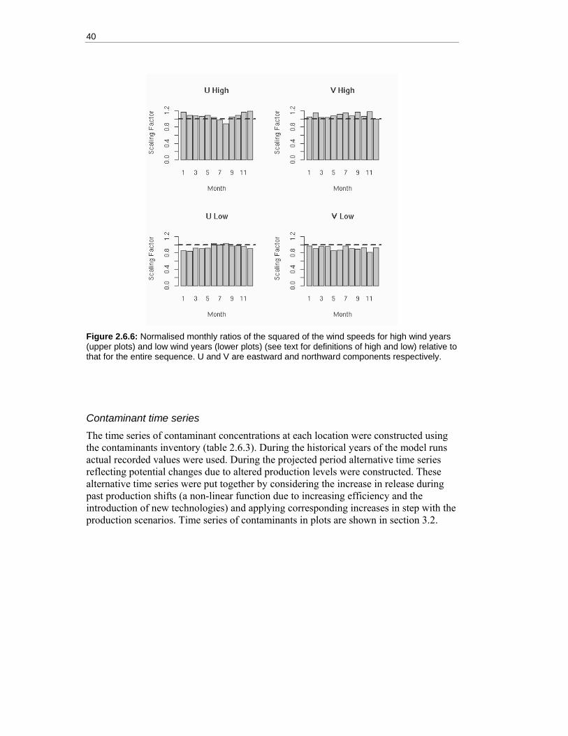
40
Figure 2.6.6: Normalised monthly ratios of the squared of the wind speeds for high wind years (upper plots) and low wind years (lower plots) (see text for definitions of high and low) relative to that for the entire sequence. U and V are eastward and northward components respectively.
Contaminant time series The time series of contaminant concentrations at each location were constructed using the contaminants inventory (table 2.6.3). During the historical years of the model runs actual recorded values were used. During the projected period alternative time series reflecting potential changes due to altered production levels were constructed. These alternative time series were put together by considering the increase in release during past production shifts (a non-linear function due to increasing efficiency and the introduction of new technologies) and applying corresponding increases in step with the production scenarios. Time series of contaminants in plots are shown in section 3.2.
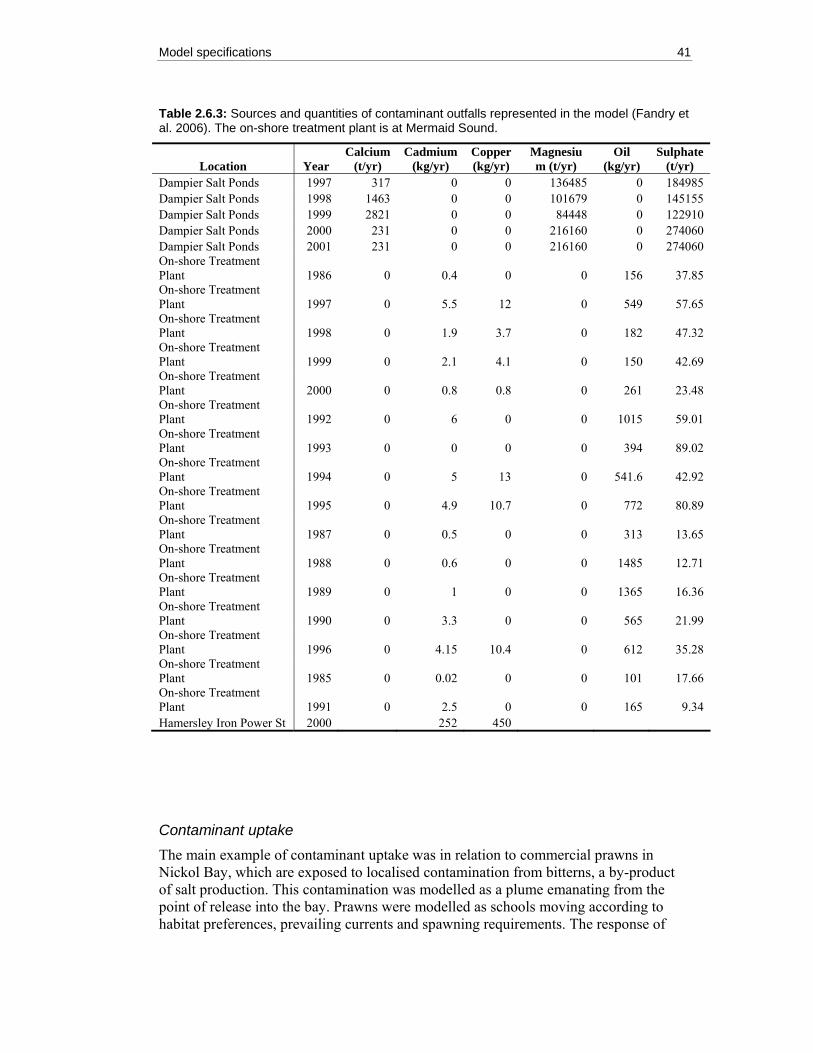
Model specifications 41
Table 2.6.3: Sources and quantities of contaminant outfalls represented in the model (Fandry et al. 2006). The on-shore treatment plant is at Mermaid Sound.
Location Year Calcium
(t/yr) Cadmium
(kg/yr) Copper(kg/yr)
Magnesium (t/yr)
Oil (kg/yr)
Sulphate (t/yr)
Dampier Salt Ponds 1997 317 0 0 136485 0 184985 Dampier Salt Ponds 1998 1463 0 0 101679 0 145155 Dampier Salt Ponds 1999 2821 0 0 84448 0 122910 Dampier Salt Ponds 2000 231 0 0 216160 0 274060 Dampier Salt Ponds 2001 231 0 0 216160 0 274060 On-shore Treatment Plant 1986 0 0.4 0 0 156 37.85 On-shore Treatment Plant 1997 0 5.5 12 0 549 57.65 On-shore Treatment Plant 1998 0 1.9 3.7 0 182 47.32 On-shore Treatment Plant 1999 0 2.1 4.1 0 150 42.69 On-shore Treatment Plant 2000 0 0.8 0.8 0 261 23.48 On-shore Treatment Plant 1992 0 6 0 0 1015 59.01 On-shore Treatment Plant 1993 0 0 0 0 394 89.02 On-shore Treatment Plant 1994 0 5 13 0 541.6 42.92 On-shore Treatment Plant 1995 0 4.9 10.7 0 772 80.89 On-shore Treatment Plant 1987 0 0.5 0 0 313 13.65 On-shore Treatment Plant 1988 0 0.6 0 0 1485 12.71 On-shore Treatment Plant 1989 0 1 0 0 1365 16.36 On-shore Treatment Plant 1990 0 3.3 0 0 565 21.99 On-shore Treatment Plant 1996 0 4.15 10.4 0 612 35.28 On-shore Treatment Plant 1985 0 0.02 0 0 101 17.66 On-shore Treatment Plant 1991 0 2.5 0 0 165 9.34 Hamersley Iron Power St 2000 252 450
Contaminant uptake The main example of contaminant uptake was in relation to commercial prawns in Nickol Bay, which are exposed to localised contamination from bitterns, a by-product of salt production. This contamination was modelled as a plume emanating from the point of release into the bay. Prawns were modelled as schools moving according to habitat preferences, prevailing currents and spawning requirements. The response of
42
prawns to the bittern plumes was assumed to be neutral in the sense that they were neither repelled nor attracted to the plume.
Measurements of contaminant levels in the water and prawns from two aquaculture ponds (referred to as A and B) recorded over six years by Hashmi et al. (2002) were used to calibrate uptake by the modelled prawns. The contaminants selected were lead, cadmium and copper. Nonlinear uptake rate parameters were chosen for each metal that produced profiles comparable to those in the prawn samples over a six year simulation.
2.7 Human behaviour Human behaviour and the effects of human activities on the marine environment were represented in the MSE using a combination of analytical decision models, response functions, specified rules, historical data and scenarios. Whether the decisions are modelled explicitly or are specified as feedback rules or scenarios, uncertainty plays an important part in determining whether human activities interact with biota and produce an environmental effect. The representation of real ecosystem behaviour and response used in the MSE (Gray et al. 2006) preserves the uncertainty that truly exists when humans attempt to achieve particular objectives (e.g. catching fish) but may fail because their observations are subject to error and because animals move or natural events (e.g. tropical cyclones) change circumstances unpredictably. Human effects are therefore represented in terms of potential interaction between humans and the environmental entities affected by, and affecting, humans.
Analytical decision models were developed for economic activities in the oil and gas industries and in the fisheries. Initially an economic model was developed for petroleum exploration and production, but could not be implemented because data needed for calibration and validation were commercially confidential. Instead, oil and gas production was introduced to the analysis by way of the development scenarios specified in section 3 below. Development scenarios were also used to specify impacts of recreational fishers, changes to port capacity, industrial production and associated contaminants, dredging, and human population dynamics.
A Bayesian decision model was used to represent finfish trawl fishing (Gray et al. 2006). This model emulated fishers’ decisions on where to fish and when to return to port. These decisions utilised historical fishing data (as a proxy for fishers’ knowledge) and the current catch to select target fishing locations, reference points and decision rules for changing location or returning to port. Each vessel spatially allocated their fishing effort based on their own internal representation of the spatial distribution of the state of the fish resource (modelled on a 1 degree grid). Within the grid cell that was deemed to have the highest expected catch rate, trawl shot and trap placement locations and vectors were selected randomly from a record of previous trawl shots that started in the grid cell. The state of the fish resource in each cell internal to each fishing operator was maintained and updated using a Kalman filter. Updates (using the numerical likelihood) were made on each occasion that the grid cell was fished.
Detailed decision modelling was also done for the fishery management authority (FMA) represented in the model (Gray et al. 2006). This involved formal stock assessments and specified decision rules for the FMA to adjust fishing effort quotas in the various fishing zones so as to serve the objectives of sustaining fish stocks and the commercial viability of the fishing industry. Formal models were not developed for other human
Model specifications 43
decisions, although feedback rules were developed for port authorities, the EPA, conservation managers and shipping vessels (Gray et al. 2006).
As noted above, the impacts captured by the model included habitat damage and fish catch (sections 2.3 to 2.5), which were represented respectively as percentage of habitat destroyed and as catchability and fishing mortality of fish schools and iconic species that come into contact with the nets. In the case of industrial production, impact is by way of the effects of contaminants on biota (section 2.6) and the effects of shipping and port development.
2.8 Physical data inputs This section describes a range of additional physical data that was used in the MSE modelling.
Bathymetry The Auslig 250k series 1 topograpic data (Geoscience Australia, 2000) was used along with a North West Shelf coastline contour to generate a 0.008 degree grid using the ArcInfo topogrid command. This was merged with the AGSO bathymetric 30 second grid ( CGeoscience Australia, 1998C) to form a complete bathymetric and topographic grid at 0.008 degree resolution for the complete North West Shelf study area (figure 2.8.1). Finally, this grid was projected to a Lambert Conformal Conic projection for use by the model. Conformal projections, ensuring that scale was invariant in all directions locally, although large grids tended to be distorted because of differential stretching of areas across large scales.

44
110o E 115o E 120o E 125o E
110o E 115o E 120o E 125o E
25o S
20o S
15o S
10o E 115o E 120o E 125o E
25o S
20o S
15o S
10o E 115o E 120o E 125o E
0 600 1200
Depth (m)
116o 30 / E 117o E
116o 30 / E 117o E
20o 30 / S
116o 30 / E 117o E
20o 30 / S
116o 30 / E 117o E
0 25 50
Depth (m)
Figure 2.8.1: Model grids (left) and model bathymetry (right) for the larger Northwest region (top) and the Dampier region (bottom). In each case, the model bathymetry was derived by averaging the Geosciences Australia product within each model grid.
Winds Wind is the predominant driver of low frequency (sub-tidal) currents on the shelf, particularly in near-surface waters. The stress τ exerted on the water surface by the wind is a quadratic function of wind speed and was estimated as:
210UCDρτ = ,
where ρ is the density of air (1.3 kg/mP
3P), UB10B is wind speed at 10 metres above
sealevel, and CBDB is the drag coefficient. The wind speed data where taken from a 40-year reanalysis of global atmospheric model fields produced by NCEP and NCAR (Kalnay et al. 1996). From this zonal and meridonal wind-stress fields on the North West Shelf were calculated for the period 1965 to 1997.
Model specifications 45
Cyclones Cyclone tracks were constructed using data supplied by the National Climate Centre in the Head Office of the Bureau of Meteorology (HTUhttp://www.bom.gov.au/UTH). These records contained information on the timing, route and intensity of cyclones, with high quality data available subsequent to the advent of GPS and automated monitoring. The final footprint of the cyclone used by the catastrophe agents in InVitro was constructed by mapping a polygon over each leg of a cyclone’s route, with the track as the centreline and a width of 30 km on either side of that central track. These footprints and an intensity index (from the original record) were stored and accessed as needed.
Rainfall The daily rainfall time series were constructed from records at Karratha and Port Hedland airports supplied by the National Climate Centre in the Bureau of Meteorology (P. Reid pers. comm.). These data sets ran from 14/12/1971 for Karratha and from 17/7/1942 for Port Hedland. These data sets were merged using: • an average where a valid entry existed for both time series; • the data as supplied if only one valid entry was present; • the long term average for that day of the year if no valid entry was present in
either time series.
The resulting combined rainfall time-series was then converted into 90-day running sums. Sums rather than averages were used as overall input to the system. These data were of particular significance to recruitment in the prawn fisheries of the region.
Light Light time series were not used within this implementation of NWS-InVitro. In its place a simple equation was used to give average light levels derived from the output of the biogeochemical model of Herzfeld et al. (2006). The formulation used for photosynthetically active radiation (PAR) at the depth of the primary producers was:
( )mII topbot ⋅−⋅= γexp ;
where m is depth in metres, the PAR at the seas surface (Itop B) is set to 170 WmP
-2P (the
long-term average taken from representative runs of the Herzfeld et al. (2006) model) and the extinction coefficient is given by
pmdmmw ,,, *0035.0*0038.0 φφφγ ++= ;
with φBw,m Bthe coefficient of background light absorption due to water, dissolved organic nutrients and inorganic suspended sediment combined (set to 0.055 for offshore waters and 0.1 for turbid inshore waters (Frost 1987; Murray & Parslow 1997)); 0.0038 is the coefficient of light absorption due to labile detritus (highly turbid values from Murray & Parslow 1997); 0.0035 is the coefficient of light absorption due to particulate matter (Tett 1990); φBm,p Bis the average concentration of particulate matter (plankton) in the water column at depth m (mg N mP
-3P); and φBm,d B is the average concentration of labile

46
detritus in the water column at depth at depth m (mg N mP
-3P). These average
concentrations were estimated from the model of Herzfeld et al. (2002):
⎩⎨⎧ >
=
⎩⎨⎧ >
=
otherwise 8650mdepth 11
otherwise 5650mdepth 7
..
.
,
,
pm
dm
φ
φ
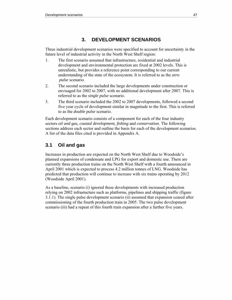
Development scenarios 47
3. DEVELOPMENT SCENARIOS
Three industrial development scenarios were specified to account for uncertainty in the future level of industrial activity in the North West Shelf region: 1. The first scenario assumed that infrastructure, residential and industrial
development and environmental protection are fixed at 2002 levels. This is unrealistic, but provides a reference point corresponding to our current understanding of the state of the ecosystem. It is referred to as the zero pulse scenario.
2. The second scenario included the large developments under construction or envisaged for 2002 to 2007, with no additional development after 2007. This is referred to as the single pulse scenario.
3. The third scenario included the 2002 to 2007 developments, followed a second five year cycle of development similar in magnitude to the first. This is referred to as the double pulse scenario.
Each development scenario consists of a component for each of the four industry sectors oil and gas, coastal development, fishing and conservation. The following sections address each sector and outline the basis for each of the development scenarios. A list of the data files cited is provided in Appendix A.
3.1 Oil and gas
Increases in production are expected on the North West Shelf due to Woodside’s planned expansions of condensate and LPG for export and domestic use. There are currently three production trains on the North West Shelf with a fourth announced in April 2001 which is expected to process 4.2 million tonnes of LNG. Woodside has predicted that production will continue to increase with six trains operating by 2012 (Woodside April 2001).
As a baseline, scenario (i) ignored these developments with increased production relying on 2002 infrastucture such as platforms, pipelines and shipping traffic (figure 3.1.1). The single pulse development scenario (ii) assumed that expansion ceased after commissioning of the fourth production train in 2005. The two pulse development scenario (iii) had a repeat of this fourth train expansion after a further five years.

48
Figure 3.1.1: Oil and gas production time series corresponding to the three development scenarios (S0P = zero pulse scenario, S1P = single pulse scenario, and S2P = double pulse scenario). The top panel is the total number of vessels (related to the oil and gas sector); the middle panel is the total human population; and the bottom panel is the total production multiplier used to estimate oil and gas production.
3.2 Coastal development For the purposes of this project coastal development includes, port facilities and shipping traffic, iron ore, salt and gas freight, on-shore gas processing plants, population, salt production, residential development, public and private infrastructure and electricity generation.
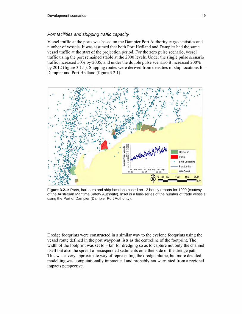
Development scenarios 49
Port facilities and shipping traffic capacity Vessel traffic at the ports was based on the Dampier Port Authority cargo statistics and number of vessels. It was assumed that both Port Hedland and Dampier had the same vessel traffic at the start of the projection period. For the zero pulse scenario, vessel traffic using the port remained stable at the 2000 levels. Under the single pulse scenario traffic increased 50% by 2005, and under the double pulse scenario it increased 200% by 2012 (figure 3.1.1). Shipping routes were derived from densities of ship locations for Dampier and Port Hedland (figure 3.2.1).
Figure 3.2.1: Ports, harbours and ship locations based on 12 hourly reports for 1999 (coutesy of the CAustralian Maritime Safety AuthorityC). Inset is a time-series of the number of trade vessels using the Port of Dampier (Dampier Port Authority).
Dredge footprints were constructed in a similar way to the cyclone footprints using the vessel route defined in the port waypoint lists as the centreline of the footprint. The width of the footprint was set to 3 km for dredging so as to capture not only the channel itself but also the spread of resuspended sediments on either side of the dredge path. This was a very approximate way of representing the dredge plume, but more detailed modelling was computationally impractical and probably not warranted from a regional impacts perspective.
020406080
100120140160180200
Jan88-89
Sept May Jan93-94
Sept May Jan98-99
Sept
Num
ber T
rade
Ves
sels
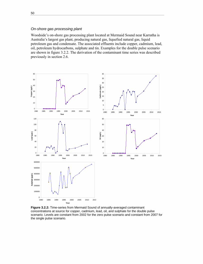
50
On-shore gas processing plant Woodside’s on-shore gas processing plant located at Mermaid Sound near Karratha is Australia’s largest gas plant, producing natural gas, liquefied natural gas, liquid petroleum gas and condensate. The associated effluents include copper, cadmium, lead, oil, petroleum hydrocarbons, sulphate and tin. Examples for the double pulse scenario are shown in figure 3.2.2. The derivation of the contaminant time series was described previously in section 2.6.
0
10
20
30
40
50
60
1980 1985 1990 1995 2000 2005 2010 2015
Year
Copp
er (µ
g/L)
0
5
10
15
20
25
30
35
40
1980 1985 1990 1995 2000 2005 2010 2015
Year
Cadm
ium
(µg/
L)
0
20
40
60
80
100
120
1980 1985 1990 1995 2000 2005 2010 2015
Year
Lead
(µg/
L)
0
10
20
30
40
50
60
1980 1985 1990 1995 2000 2005 2010 2015
Year
Oil
(µg/
L)
0
100000
200000
300000
400000
500000
600000
1980 1985 1990 1995 2000 2005 2010 2015
Year
Sul
phat
e (µ
g/L)
Figure 3.2.2: Time-series from Mermaid Sound of annually-averaged contaminant concentrations at source for copper, cadmium, lead, oil, and sulphate for the double pulse scenario. Levels are constant from 2002 for the zero pulse scenario and constant from 2007 for the single pulse scenario.

Development scenarios 51
Salt production The Pilbara salt ponds are a major producer of commercial sodium chloride producing seven million tonnes per year. The two producers are Dampier Salt, operating at Port Hedland and Dampier, and Onslow Salt. The residual brine is called bitterns and contains calcium, sulphate chloride of magnesium, bromine, iodine and potassium. The magnesium is used here as an indicator for bitterns.
For the single pulse scenario salt production is assumed to increase over the five year period from 2002 to 2007 then remains constant till 2012. For the double pulse scenario the projected increase is extended until 2012. The projected increases for each development scenario were derived from actual increases experienced by the industry in the period prior to 2002.
Iron ore and electricity generation The impacts of increased electricity and iron ore production can be linked to increased effluents. The effluents from these industries include zinc, lead, copper, chromium and cadmium (Revill, 2002; Fandry et al. 2006). However, this study looked only at the copper discharged from these industries because it has the highest potential ecological impact. From 2002 copper discharges increased following the same scenario trends as described above for gas processing and salt production (figure 3.2.3).
0
20
40
60
80
100
120
1980 1985 1990 1995 2000 2005 2010 2015
Year
Copp
er (µ
g/L)
Figure 3.2.3: Copper contaminant time-series from Hammersley Iron.
Human Populations The population distribution in the Pilbara region based on the 2001 census is shown in figures 3.2.4 and 3.2.5. Human population time series and projections for each population centre along the Pilbara coast were downloaded from the Australia Bureau

52
of Statistics Census website (HTUhttp://www.abs.gov.auUTH). The ports included explicitly in the model were Dampier, Exmouth, Onslow, Point Samson, and Port Hedland. However, due to the potential for pressures (e.g. recreational fishing) to flow from locations further inland (e.g. Karratha), their populations were factored into the population time series of the adjacent port site. Figure 3.2.6 shows the example of Port Hedland population growth for the three development scenarios.
Figure 3.2.4: Population density by census collector district in persons per square km (Australian Bureau of Statistics 2001).
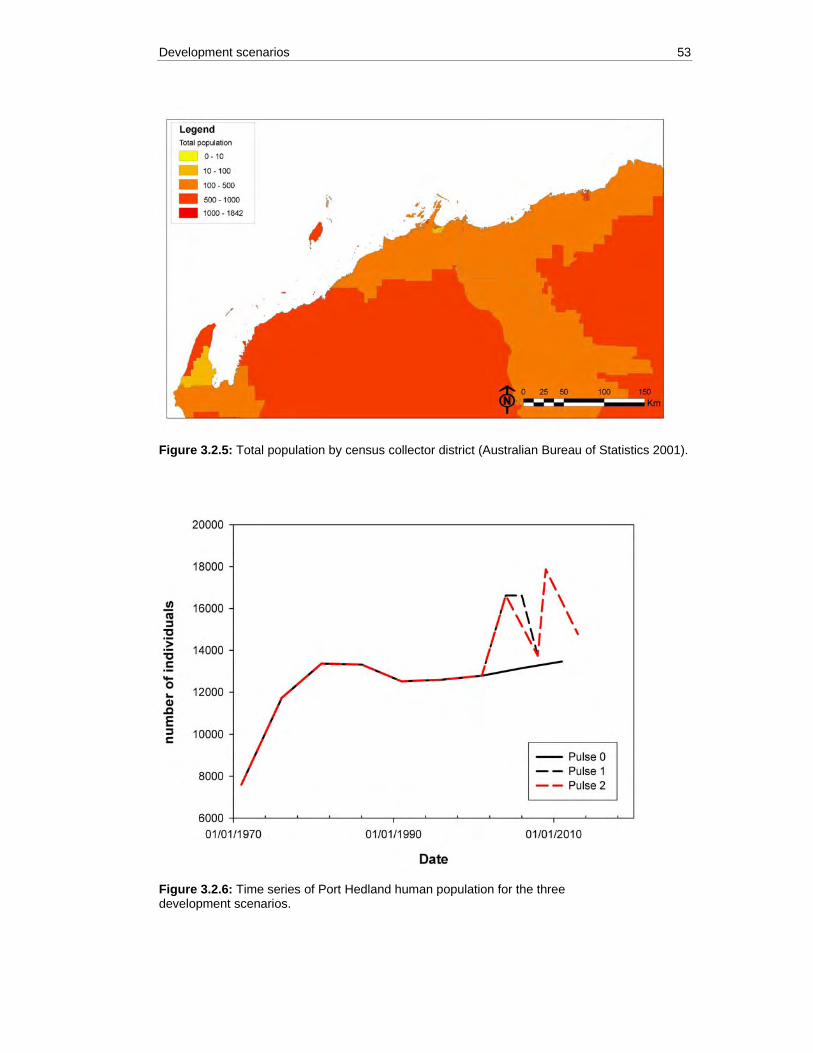
Development scenarios 53
Figure 3.2.5: Total population by census collector district (Australian Bureau of Statistics 2001).
Figure 3.2.6: Time series of Port Hedland human population for the three development scenarios.

54
3.3 Fishing sector The fishing sector is made up of commercial and recreational fishing. The form of management in this sector means that only relatively modest changes in pressure would be plausible. Consequently, this study considered just one development scenario for the fishing sector with the number of vessels being: • six trawlers located at Point Sampson; • one trap fisher located at Point Sampson; • 28 prawn trawlers located in Exmouth; • 16 prawn fishers located in Onslow; and • 26 prawn fishers located in Dampier.
The fishing effectiveness of the vessels was constant throughout the study period.
Recreational fishing in the MSE was represented using a simple constant proportion agent (Gray et al. 2006). The extent of the access of this agent to fish stocks was dependent on the road network. At any known boat ramp or any point where the road network came within one kilometre the recreational fishers were assumed to have an access point. The mortality imposed on the fish groups was inversely proportional to the distance from a human settlement site (e.g. a port) to the access point and the distance from the access point out to the fish (figure 3.9). This model was then tuned to the data from the national creel survey (Henry & Lyle, 2003) so that the numbers of fish taken in the historical part of the model matched that recorded in the creel survey.
The numbers of fish taken in the creel survey were calculated by summing the effort recorded in the tropical part of Western Australia (44693 hr/yr) and determining the proportion of that effort due to fishers in the Pilbara region (0.3625). The total catch of Red emperor (Lutjanus sebae), Lethrininds and Lutjanids were calculated as:
pilbara_catch = total WA catch x proportionof effort in pilbara
This gave monthly catches of 544 for L. Sebae, 6024 for Lethrinids and 2079 for Lutjanids.
There was no direct modification to the recreational fishing model under any management strategy or development scenario. The only changes realised in relation to recreational fishing were as a result of: • extra pressure that ensued from higher human population levels under the
alternative development scenarios; and • additional fisheries management actions (e.g. closed areas) under the alternative
management strategies.
In the single pulse development scenario recreational fishing effectiveness (including the range of access from ports) increased by 3% per annum from 2002 to 2007. This rate of increase was maintained for a further five years for the double pulse scenario.

Development scenarios 55
Figure 3.3.1: Distribution of recreational fishing on the North West Shelf. The dark red regions are areas of high recreational fishing density.
3.4 Conservation sector The passage of the CALM Act (1984) provided statutory provision for the declaration of marine reserves for nature conservation and public recreation purposes. In the period 1987 through 1990 there were seven CALM Act marine reserves declared and one special legislation marine reserve. However none of these were located in the region of this study.
The development scenario considered for the period of the study was the region as it was in July 2002. There were no marine or coastal reserves. However, fishing zone three, prawn nursery grounds and exclusion zones around oil and gas facilities were closed to fishing and remained closed for the duration of the model runs. Many of these closed regions overlapped with the areas identified by the Wilson report (figure 3.4.1).
Additional closures to fishing occurred through the implementation of the enhanced and integrated management strategies (see sections 4.2 and 4.3). These management driven closures were in response to the stocks of turtles or sharks falling below 20% of initial biomass (see section 2.4).
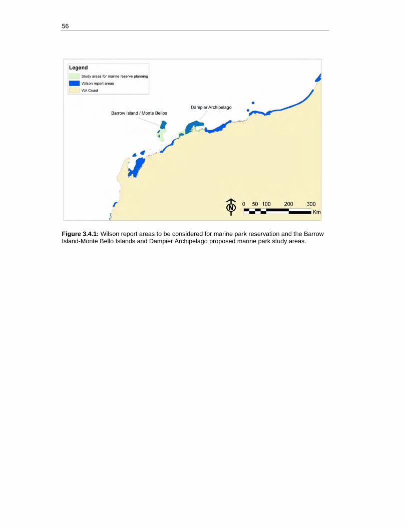
56
Figure 3.4.1: Wilson report areas to be considered for marine park reservation and the Barrow Island-Monte Bello Islands and Dampier Archipelago proposed marine park study areas.
Management strategies 57
4. MANAGEMENT STRATEGIES
The three management strategies chosen for evaluation are closely aligned to existing sector-by-sector legislative requirements. The first management strategy is referred to as the status quo because it broadly represents the combination of sectoral management strategies in place in 2002. These are detailed in gazetted legislation and associated regulations for departments and local authorities (Gordon, 2006).
The second management strategy examined is referred to as the enhanced management strategy because it includes potential modifications to the existing sectoral strategies that might allow some management objectives to be met more effectively. In particular the enhanced strategies make increased use of monitoring to measure the condition of the environment and resource used by each sector, and of remedial action if this monitoring indicates undesirable outcomes.
The third and final strategy examined is referred to as the regionally co-ordinated sectoral strategy. It is based on the existence of a regional mechanism to establish indicators and benchmarks, to coordinate monitoring, to enable the results of monitoring and assessment to be shared across sectors, and to facilitate a multi-sectoral management response if undesirable trends were detected in monitored indicators. Otherwise sectoral strategies operated as per the enhanced strategies above.
The objectives of all sectoral management strategies include the achievement of Ecologically Sustainable Development, as outlined in the Inter-governmental Agreement on the Environment (IGAE) (Commonwealth of Australia 1992) and the National Strategy for ESD (Commonwealth of Australia 1992), as well as the requirements of numerous pieces of relevant legislation (see, for example, the review of legislation affecting human activities related to the North West Shelf marine ecosystem by Gordon, 2006). The objective of ESD is “using, conserving and enhancing the community’s resources so that ecological processes, on which life depends, are maintained, and the total quality of life, now and in the future, can be increased” (Commonwealth of Australia 1992). The principles of ESD as expressed in the IGAE include: • international competitiveness should be maintained and enhanced in an
environmentally sound manner; • environmental considerations will be integrated into all government decision
making, and this should include proper and cost-effective examination of matters that significantly affect the environment;
• conservation of biological diversity and ecological integrity are fundamental considerations in decision making;
• the precautionary approach should be applied in decision making; • inter-generational equity is provided through ensuring the health, diversity and
productivity of the environment; and • there should be valuation, pricing and incentive mechanisms to achieve
environmental goals.
These are taken to be the over-arching objectives and principles that management strategies are seeking to meet. The effectiveness of implementation of management

58
measures was assumed to be imperfect, but the same under all strategies for each sector. For each sector this imperfect implementation comprised: • oil and gas effluent limits were adhered to on 80% of the occasions when
operationally they could be exceeded; • coastal development effluent limits were adhered to on 80% of the occasions
when operationally they could be exceeded; • commercial fisheries catch records were provided accurately on 80% of
occasions, while recreational fishing bag limits were adhered to on 75% of occasions when operationally they could be exceeded. Both commercial and recreational fishing operations were located within appropriate zones (e.g. fishery management zones and exclusion zones for management of other sectors) on 95% of occasions; and
• conservation controls on icon species and MPA conditions were adhered to by 80% of operations that could violate the conditions or controls.
The three strategies will now be described for each of the sectors oil and gas, coastal development, fishing and conservation. However, all sectors will treated together when describing the regionally coordinated sectoral strategy.
4.1 Oil and gas Management of oil and gas production is the joint responsibility of the Australian Federal Government (Commonwealth of Australia (1967) Petroleum (Submerged Lands) Act 1967) and Western Australian state government (Government of Western Australia (1982) Petroleum (Submerged Lands) Act 1982). This extends from exploration activities through to construction of production and processing facilities, as well as ongoing activities related to resource extraction, processing and transport.
Exploration and production were initially represented as sequential joint production processes within the MSE modelling (NWSJEMS interim report 2002). This involved modelling the economic decisions of petroleum firms so that company responses to management changes could be included in the MSE. Unfortunately, commercial confidentiality prevented adequate calibration and testing of this model component, so it was excluded from the analysis. Instead oil and gas production were treated as scenarios and it was assumed that compliance with production and environmental regulations is a natural and voluntary part of the productive activities of petroleum firms.
Status quo strategy As of July 2002, management of the production phase of oil and gas extraction was principally concerned with occupational and public safety and the release of contaminants into the environment. The Environmental Protection Authority has the responsibility for preventing, controlling and abating environmental pollution (Government of Western Australia (1986-93) Environmental Protection Act 1986-93). In addition there is a social welfare or resource rents aspect that requires petroleum firms to use procedures and technologies that maximise the quantity of oil and gas extracted from each proven reserve.
Release of contaminants of various types is regulated by volume and concentration. Discharges of this type include produced formation water (PFW) which is a by-product
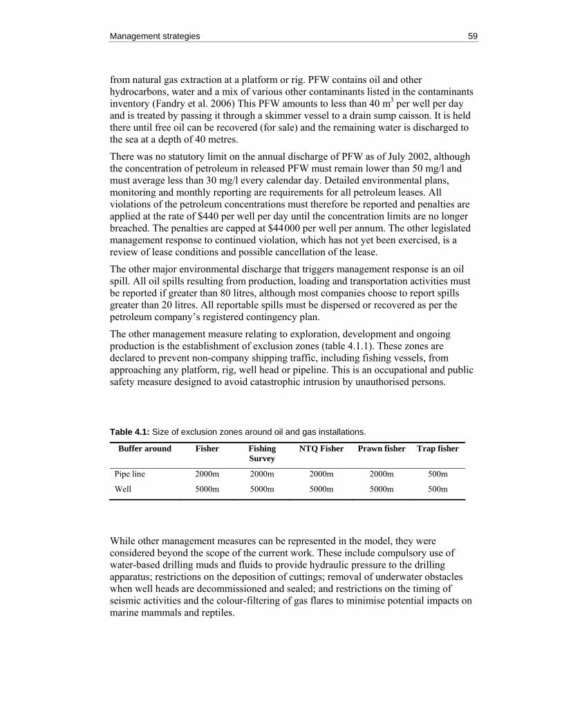
Management strategies 59
from natural gas extraction at a platform or rig. PFW contains oil and other hydrocarbons, water and a mix of various other contaminants listed in the contaminants inventory (Fandry et al. 2006) This PFW amounts to less than 40 mP
3P per well per day
and is treated by passing it through a skimmer vessel to a drain sump caisson. It is held there until free oil can be recovered (for sale) and the remaining water is discharged to the sea at a depth of 40 metres.
There was no statutory limit on the annual discharge of PFW as of July 2002, although the concentration of petroleum in released PFW must remain lower than 50 mg/l and must average less than 30 mg/l every calendar day. Detailed environmental plans, monitoring and monthly reporting are requirements for all petroleum leases. All violations of the petroleum concentrations must therefore be reported and penalties are applied at the rate of $440 per well per day until the concentration limits are no longer breached. The penalties are capped at $44 000 per well per annum. The other legislated management response to continued violation, which has not yet been exercised, is a review of lease conditions and possible cancellation of the lease.
The other major environmental discharge that triggers management response is an oil spill. All oil spills resulting from production, loading and transportation activities must be reported if greater than 80 litres, although most companies choose to report spills greater than 20 litres. All reportable spills must be dispersed or recovered as per the petroleum company’s registered contingency plan.
The other management measure relating to exploration, development and ongoing production is the establishment of exclusion zones (table 4.1.1). These zones are declared to prevent non-company shipping traffic, including fishing vessels, from approaching any platform, rig, well head or pipeline. This is an occupational and public safety measure designed to avoid catastrophic intrusion by unauthorised persons.
Table 4.1: Size of exclusion zones around oil and gas installations.
Buffer around Fisher Fishing Survey
NTQ Fisher Prawn fisher Trap fisher
Pipe line 2000m 2000m 2000m 2000m 500m
Well 5000m 5000m 5000m 5000m 500m
While other management measures can be represented in the model, they were considered beyond the scope of the current work. These include compulsory use of water-based drilling muds and fluids to provide hydraulic pressure to the drilling apparatus; restrictions on the deposition of cuttings; removal of underwater obstacles when well heads are decommissioned and sealed; and restrictions on the timing of seismic activities and the colour-filtering of gas flares to minimise potential impacts on marine mammals and reptiles.
60
Enhanced management strategy The monitoring component of the enhanced management strategy entails measurement of the accumulation of key contaminants in oysters within 1 km of installations (Cu, CaSO B4 B, lead, oil as an indictor for PFW, and magnesium as an indictor for bitterns), as well as monitoring species richness. Management responses were triggered at half the ANZECC guidelines (with the aim of avoiding reaching the guideline levels) or by a rapid decline in turtle or shark populations.
The management response was a requirement that contaminant outputs be reduced by 50%. The cost of this improvement was A$25M over the first five years and A$2M pa thereafter. Success in achieving the target reductions in contaminant output after five years was assumed, in even intervals of reduction. The management response could be repeated at five year intervals if monitoring continued to show undesirable outcomes. While production levels were not changed by triggered remedial actions, the effective production was reduced by EPA restrictions regarding contaminant outflows.
4.2 Coastal Development
Status quo strategy Management of the coastal zone is conducted through a combination of uniform ANZECC/ARMCANZ (2000) water quality standards ( HTUhttp://www.deh.gov.au/water/quality/nwqms/index.html)H and zoning for industrial, residential and recreational development (Government of Western Australia (1985) Western Austrlain planning Commission Act 1985). As at July 2002 the Department of Environmental Protection (DEP) (Government of Western Australia (1986-93) Environmental Protection Act 1986-93) adopted ANZECC/ ARMCANZ (2000) guidelines for water quality, food quality and sediment composition. These were incorporated into all development plans approved for industrial, residential, tourism and recreational purposes. In addition to these standards, industrial zones were developed for Maitland (on the Burrup Peninsula), Hedland and COnslowC.
The Department of Marine and Harbours (Government of Western Australia (1981) Marine and Harbours Act 1981; Government of Western Australia (1967) Shipping and Pilotage Act 1967; Government of Western Australia (1982) Western Australia Marine Act 1982; Government of Western Australia (1981) Prevention of a Collision at Sea regulations 1983) and local port authorities (Government of Western Australia (1985) Dampier Port Authority Act 1985) monitor and regulate shipping transport. Their main responsibility is to monitor port usage and profit, ensuring port facilities can handle the traffic demanded by the economic conditions.
Safety incidents are also investigated and records maintained of near misses. The number of times vessels in the model needed to take evasive manoeuvres to prevent a collision was similarly recorded and used as an indicator of the likelihood of a vessel collision and possible spill. However, under the status quo management strategy this data did not trigger any management action, with port capacity being held constant.
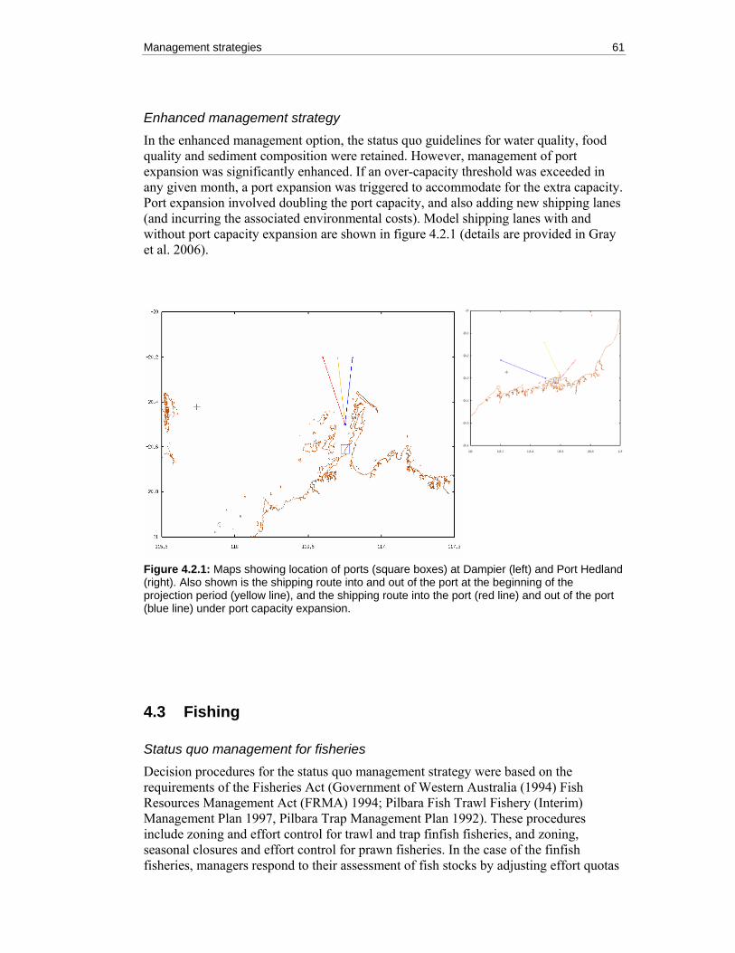
Management strategies 61
Enhanced management strategy In the enhanced management option, the status quo guidelines for water quality, food quality and sediment composition were retained. However, management of port expansion was significantly enhanced. If an over-capacity threshold was exceeded in any given month, a port expansion was triggered to accommodate for the extra capacity. Port expansion involved doubling the port capacity, and also adding new shipping lanes (and incurring the associated environmental costs). Model shipping lanes with and without port capacity expansion are shown in figure 4.2.1 (details are provided in Gray et al. 2006).
Figure 4.2.1: Maps showing location of ports (square boxes) at Dampier (left) and Port Hedland (right). Also shown is the shipping route into and out of the port at the beginning of the projection period (yellow line), and the shipping route into the port (red line) and out of the port (blue line) under port capacity expansion.
4.3 Fishing
Status quo management for fisheries Decision procedures for the status quo management strategy were based on the requirements of the Fisheries Act (Government of Western Australia (1994) Fish Resources Management Act (FRMA) 1994; Pilbara Fish Trawl Fishery (Interim) Management Plan 1997, Pilbara Trap Management Plan 1992). These procedures include zoning and effort control for trawl and trap finfish fisheries, and zoning, seasonal closures and effort control for prawn fisheries. In the case of the finfish fisheries, managers respond to their assessment of fish stocks by adjusting effort quotas
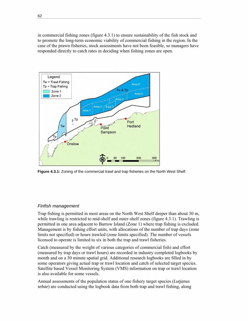
62
in commercial fishing zones (figure 4.3.1) to ensure sustainability of the fish stock and to promote the long-term economic viability of commercial fishing in the region. In the case of the prawn fisheries, stock assessments have not been feasible, so managers have responded directly to catch rates in deciding when fishing zones are open.
Figure 4.3.1: Zoning of the commercial trawl and trap fisheries on the North West Shelf.
Finfish management Trap fishing is permitted in most areas on the North West Shelf deeper than about 30 m, while trawling is restricted to mid-shelf and outer-shelf zones (figure 4.3.1). Trawling is permitted in one area adjacent to Barrow Island (Zone 1) where trap fishing is excluded. Management is by fishing effort units, with allocations of the number of trap days (zone limits not specified) or hours trawled (zone limits specified). The number of vessels licensed to operate is limited to six in both the trap and trawl fisheries.
Catch (measured by the weight of various categories of commercial fish) and effort (measured by trap days or trawl hours) are recorded in industry completed logbooks by month and on a 30 minute spatial grid. Additional research logbooks are filled in by some operators giving actual trap or trawl location and catch of selected target species. Satellite based Vessel Monitoring System (VMS) information on trap or trawl location is also available for some vessels.
Annual assessments of the population status of one fishery target species (Lutjanus sebae) are conducted using the logbook data from both trap and trawl fishing, along
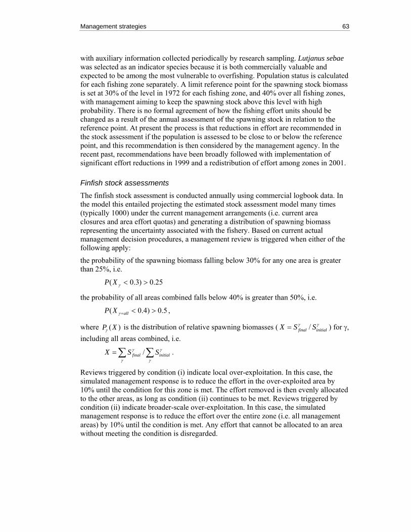
Management strategies 63
with auxiliary information collected periodically by research sampling. Lutjanus sebae was selected as an indicator species because it is both commercially valuable and expected to be among the most vulnerable to overfishing. Population status is calculated for each fishing zone separately. A limit reference point for the spawning stock biomass is set at 30% of the level in 1972 for each fishing zone, and 40% over all fishing zones, with management aiming to keep the spawning stock above this level with high probability. There is no formal agreement of how the fishing effort units should be changed as a result of the annual assessment of the spawning stock in relation to the reference point. At present the process is that reductions in effort are recommended in the stock assessment if the population is assessed to be close to or below the reference point, and this recommendation is then considered by the management agency. In the recent past, recommendations have been broadly followed with implementation of significant effort reductions in 1999 and a redistribution of effort among zones in 2001.
Finfish stock assessments The finfish stock assessment is conducted annually using commercial logbook data. In the model this entailed projecting the estimated stock assessment model many times (typically 1000) under the current management arrangements (i.e. current area closures and area effort quotas) and generating a distribution of spawning biomass representing the uncertainty associated with the fishery. Based on current actual management decision procedures, a management review is triggered when either of the following apply:
the probability of the spawning biomass falling below 30% for any one area is greater than 25%, i.e.
25.0)3.0( ><γXP
the probability of all areas combined falls below 40% is greater than 50%, i.e.
5.0)4.0( ><=allXP γ ,
where ( )P Xγ is the distribution of relative spawning biomasses ( /final initialX S Sγ γ= ) for γ, including all areas combined, i.e.
/final initialX S Sγ γ
γ γ
= ∑ ∑ .
Reviews triggered by condition (i) indicate local over-exploitation. In this case, the simulated management response is to reduce the effort in the over-exploited area by 10% until the condition for this zone is met. The effort removed is then evenly allocated to the other areas, as long as condition (ii) continues to be met. Reviews triggered by condition (ii) indicate broader-scale over-exploitation. In this case, the simulated management response is to reduce the effort over the entire zone (i.e. all management areas) by 10% until the condition is met. Any effort that cannot be allocated to an area without meeting the condition is disregarded.

64
Prawn management The three North West Shelf prawn fisheries are the Exmouth Gulf Prawn Fishery, the Onslow Prawn Fishery and the Nickol Bay Prawn Fishery. In reality, each fishery is spatially managed with openings and closures of multiple zones (figure 4.3.2). The fisheries are not independent, with effort levels in the Onslow and Nickol Bay fisheries being dependent on the Exmouth Gulf fishery.
Figure 4.3.2: Prawn fishery management zones for Exmouth Gulf (left), Onslow and Nickol Bay (right).
Onslow and Nickol Bay have generally produced lower catches than Exmouth (table 4.3.1) and have not required much management intervention beyond setting acceptable catch limits (table 4.3.2). In contrast, Exmouth has had a history of not only setting acceptable catch limits, but also experienced a temporary closure in 1999–2000 due to low catch rates. Reference limits in the Exmouth fishery also include acceptable catch ranges that are calculated based on historical data.
Prawn fishery management in the model consists of a decision procedure based on the total catch coming from each fishery as a performance indicator, and the projected or acceptable range limits. The procedure acts on the fishery when the performance indicators, in this case total catch, are outside of the reference limits of acceptable catch range. In reality, actual management action has not always been taken under such a circumstance, as environmental conditions have been used to explain the outlying catch record. The only instance were action has been taken was in the Exmouth Gulf fishery in 1999–2000, where areas were closed for three years following two consecutive years of low catches. The model decision procedure implemented similar restrictions, closing a randomly selected area for three years in any fishery that displayed two consecutive years of total catches below acceptable ranges.

Management strategies 65
Table 4.3.1: Historical prawn species catch data.
Actual catch data (tonnes)
Year Fishery king tiger endeavour banana total
98-99 Exmouth 508 377 170 3 1058
Onslow 35 14 11 2 61
Nickol Bay 50 3 1 36 89
99-00 Exmouth 471 451 543 2 1467
Onslow 38 26 20 9 93
Nickol Bay 69 13 5 171 259
00-01 Exmouth 299 82 122 62 565
Onslow 12 18 6 51 87
Nickol Bay 31 13 1 467 512
Table 4.3.2: Comparison of acceptable catch ranges for actual and modelled management of prawn fisheries (see Appendix C for further details).
Fishery Actual acceptable catch (tonnes)
Model acceptable catch (tonnes)
Exmouth king 350-500
tiger 250-550
endeavour 120-300
banana -
total 771-1276 350-500
Onslow king 10-55
tiger 5-40
endeavour 5-20
banana 2-90
total 60-130 57-100
Nickol Bay king 20-70
tiger 2-40
endeavour 1-10
banana 40-220
total 90-300 110-240

66
Recreational fishing The management procedures for recreational fishing, under all management strategies, included rules on discarding rates, legal size limits, prohibited species and spatial management zones. A fish could only be retained by the recreational fisher if all of these management measures allow it (i.e. it is a species that is both desirable and unprotected, of a desirable and legal size and not in a “no-take” marine protected area). The model did not provide for monitoring or assessment of stocks, and there was no planned management intervention.
Enhanced sectoral management strategy for fisheries The enhanced sectoral management strategy involved additional monitoring in the form a fishing vessel that lands a commercial catch while simultaneously providing key scientific data. In addition, for the prawn fishery, fishing ceased if CPUE fell below the lowest fishery specific CPUE in the ten years prior to the projection period of the model. This already exists on a voluntary basis in the real prawn fishery with a minimum CPUE of 16 kg/hr.
Enhanced finfish stock assessments The operations of the additional fishing vessel involved randomly selecting a trawl area and then a location within this area subject to the same constraints as regular trawl vessels. The age distributions of the catch obtained by this vessel were recorded and used to improve the biomass estimates of the stock assessment model by updating the log-likelihood of the commercial CPUE data with the log-likelihood of the age distributions:
,,,3
, ,,
ˆln
2
sa ys
age a y sy s a a y
pn pp
γγ
γλ⎛ ⎞
= ⎜ ⎟⎜ ⎟⎝ ⎠
∑ ∑ ∑ ,
where 3n is the number of years which the survey have been performed; ,,
sa yp γ is the
observed proportion of individuals in the catch of the survey vessel of sex s in year y that are age a ; and ,
,ˆ sa yp γ is the estimated proportion of individuals in the catch of the
survey vessel of sex s in year y that are age a ; i.e.
,,,
,
ˆs sa y ys
a y s sa y a
s a
N Vp
N Vγ =∑∑
The new overall log-likelihood is then CPUE ageλ λ λ= − .

Management strategies 67
4.4 Conservation Direct responsibility for conservation management rests with the Western Australian Department of Conservation and Land Management (CALM) (Government of Western Australia (1994) Conservation and Land Management Act 1994 [CALM], Government of Western Australian (1997), Acts Amendment (Marine Reserves) Act 1997, Government of Western Australian Government (1950) Wildlife Conservation Act 1950), which is responsible for protection of both terrestrial and marine fauna and flora.
As at 31 December 2002 the main instruments of conservation management were terrestrial and coastal reserves and the protection of individual species beyond these reserves. The region of North West Shelf considered by this study did not contain any coastal and marine reserves. However, fishing zone three, prawn nursery grounds, and exclusion zones around oil and gas facilities (see figure 1.2.1) were closed to fishing and remained closed for the duration of the model runs. Additional closures to fishing occurred through the implementation of the enhanced and integrated management strategies (see section 4.3). These management driven closures were in response to the stocks of turtles or sharks falling below 20% of initial biomass (see section 2.4).
4.5 Regionally coordinated sectoral management The status quo and enhanced management strategies have been described for each sector. The regionally coordinated management strategy will now be described considering all sectors simultaneously.
The regionally coordinated strategy was based on the existence of a regional mechanism to establish indicators and benchmarks, to coordinate monitoring, to enable the results of monitoring and assessment to be shared across sectors, and to facilitate a multi-sectoral management response if undesirable trends were detected in monitored indicators. Otherwise sectoral strategies operated as per the enhanced strategies described above.
The regional management response was conducted through modification of the sectoral management arrangements, rather than a requirement for new kinds of arrangements. For each indicator it is envisaged that there is prior agreement about which sectors are likely to be relevant if undesirable trends are detected, and that a multi-sector response by those sectors has been identified. A decision tree for regionally coordinated management decisions is shown in figure 4.5.1.
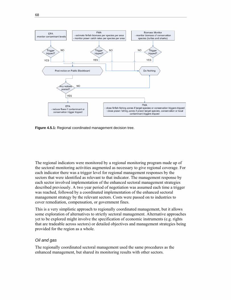
68
Figure 4.5.1: Regional coordinated management decision tree.
The regional indicators were monitored by a regional monitoring program made up of the sectoral monitoring activities augmented as necessary to give regional coverage. For each indicator there was a trigger level for regional management responses by the sectors that were identified as relevant to that indicator. The management response by each sector involved implementation of the enhanced sectoral management strategies described previously. A two year period of negotiation was assumed each time a trigger was reached, followed by a coordinated implementation of the enhanced sectoral management strategy by the relevant sectors. Costs were passed on to industries to cover remediation, compensation, or government fines.
This is a very simplistic approach to regionally coordinated management, but it allows some exploration of alternatives to strictly sectoral management. Alternative approaches yet to be explored might involve the specification of economic instruments (e.g. rights that are tradeable across sectors) or detailed objectives and management strategies being provided for the region as a whole.
Oil and gas The regionally coordinated sectoral management used the same procedures as the enhanced management, but shared its monitoring results with other sectors.
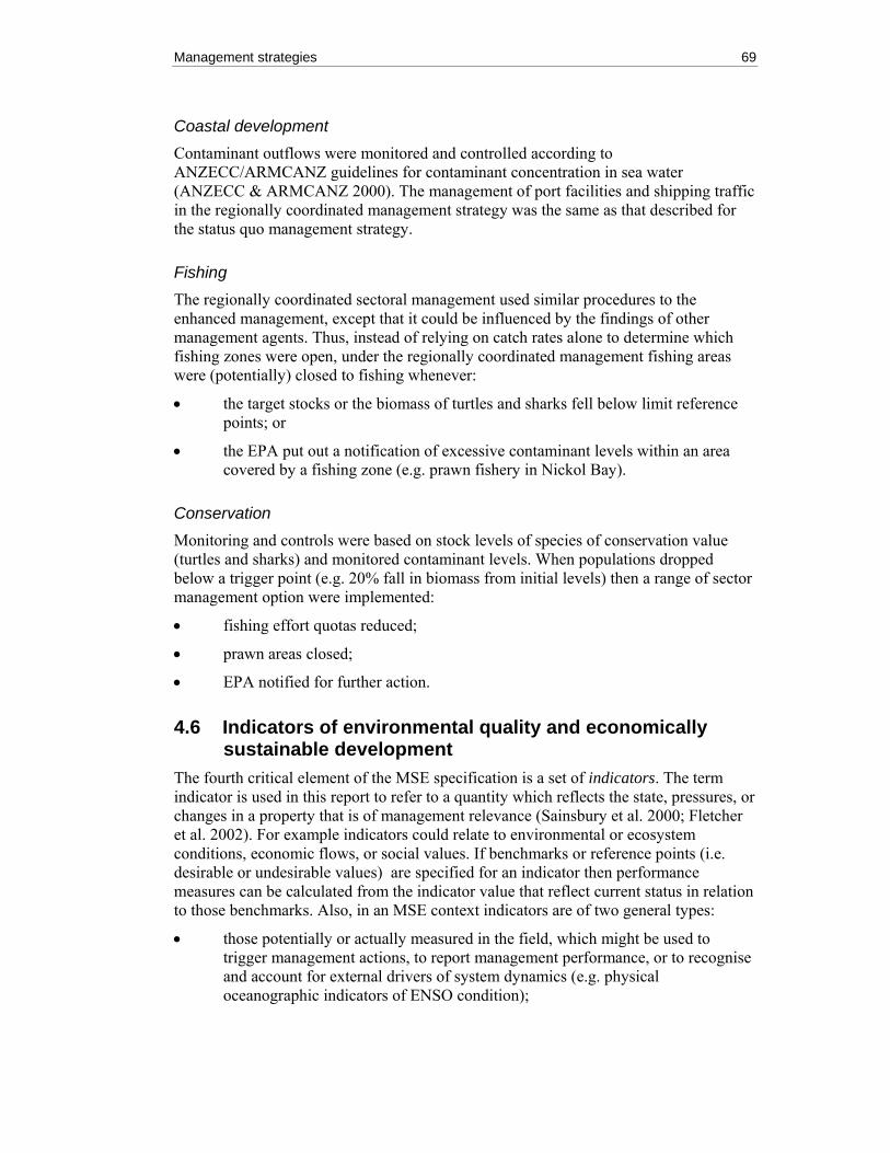
Management strategies 69
Coastal development Contaminant outflows were monitored and controlled according to ANZECC/ARMCANZ guidelines for contaminant concentration in sea water (ANZECC & ARMCANZ 2000). The management of port facilities and shipping traffic in the regionally coordinated management strategy was the same as that described for the status quo management strategy.
Fishing The regionally coordinated sectoral management used similar procedures to the enhanced management, except that it could be influenced by the findings of other management agents. Thus, instead of relying on catch rates alone to determine which fishing zones were open, under the regionally coordinated management fishing areas were (potentially) closed to fishing whenever:
• the target stocks or the biomass of turtles and sharks fell below limit reference points; or
• the EPA put out a notification of excessive contaminant levels within an area covered by a fishing zone (e.g. prawn fishery in Nickol Bay).
Conservation Monitoring and controls were based on stock levels of species of conservation value (turtles and sharks) and monitored contaminant levels. When populations dropped below a trigger point (e.g. 20% fall in biomass from initial levels) then a range of sector management option were implemented:
• fishing effort quotas reduced;
• prawn areas closed;
• EPA notified for further action.
4.6 Indicators of environmental quality and economically sustainable development
The fourth critical element of the MSE specification is a set of indicators. The term indicator is used in this report to refer to a quantity which reflects the state, pressures, or changes in a property that is of management relevance (Sainsbury et al. 2000; Fletcher et al. 2002). For example indicators could relate to environmental or ecosystem conditions, economic flows, or social values. If benchmarks or reference points (i.e. desirable or undesirable values) are specified for an indicator then performance measures can be calculated from the indicator value that reflect current status in relation to those benchmarks. Also, in an MSE context indicators are of two general types:
• those potentially or actually measured in the field, which might be used to trigger management actions, to report management performance, or to recognise and account for external drivers of system dynamics (e.g. physical oceanographic indicators of ENSO condition);

70
• those used internally to the MSE process to allow comparison the performance of the alternative strategies (potentially including aspects of a system that are important but that can not be easily measured directly in the real world).
A wide range of indicators have been proposed and evaluated for use in monitoring and managing ecosystem components. Ecological indicators are usually scale-dependent and relevant to one of the following hierarchical levels:
• individuals (behavioural and metabolic responses);
• populations (behavioural, demographic, metabolic and genetic responses of certain species);
• communities (species richness, diversity and habitat structure); and
• ecosystems (ecosystem production or trophic structure).
It has been shown that community and ecosystem level indicators are generally the most useful for monitoring ecosystem-level impacts of human activities (Frost et al. 1992; Fulton et al. 2006). However, there are notable exceptions, such as contaminant levels in individuals having broader ecological implications.
Species with particular roles or vulnerabilities (e.g. harvested, bycatch, key-stone, pest, and threatened species) may all be useful indicators (Carignan & Villard 2002; Fulton et al. 2004). Other species may be used as indicators if they are easily sampled, readily identified, cosmopolitan, or characterise system state or causes of change in a system. Any of these species are known as “indicator species”. Groups often found to be useful indicator species include seagrass, benthic invertebrates, piscivorous and planktivorous fish, and high-level predators (e.g. birds, sharks and marine mammals). Selection of key species to be monitored in any specific system must be done carefully and must span a suite of species with a range of properties, habitat requirements, sensitivities and rates of response (Whitfield & Elliott 2002; Fulton et al. 2006).
The MSE modelling used a wide range of indicators to describe outcomes and compare alternative management strategies. These are detailed below under categories such as environmental, ecological, fisheries, economic and social indicators.
Environmental indicators The environmental indicators included in the study were: • water quality in selected zones (primarily contaminant concentrations); • sediment contamination in selected zones; • contaminant concentrations in tissues (of oysters at monitored sites, prawns,
sharks and turtles); and • total contaminant exposure per unit time (of the monitored taxa).
These were monitored in specific coastal and off-shore development zones.

Management strategies 71
Ecological indicators Ecological indicators came from the evaluation of Fulton et al. (2004, 2005): • regional habitat diversity (total count of groups at a location and high and low
order Réyni and Shannon diversity measures, so both richness and evenness are considered);
• population status of k-selected indicator species (i.e. long lived species with low reproductive rates – turtles and sharks in this case);
• ratio of r-selected (short-lived with high reproduction rates) to k-selected biomass in the catch;
• status of expected sensitive or vulnerable habitat forming taxa (seagrass, mangroves, corals and sponges in this case);
• fragmentation by habitat type; and • primary productivity (satellite monitoring of Chla with some ground truthing)
with benchmarks set relating to expected eutrophication and pristine levels.
Fisheries indicators Fisheries have a long history of using indicators for monitoring and managing sector activities. The classical fisheries indicators were used here: • catch (per fleet, including recreational); • effort (per fleet, including recreational); • catch per unit effort (CPUE) (per fleet, including recreational); • target stock biomass; • bycatch rates; • bycatch stock biomass (k-selected group in the model); and • area affected by fishing (i.e. area trawled).
Economic indicators The economic indicators chosen for use in the MSE are typically widely used and well accepted: • value of production by sector and for all sectors combined; • return (gross revenue) on investment by sector and for all sectors combined; • flow of government royalties; • employment level; • per capita gross income; • throughput of ships for each port; and • number of vessel evasive manoeuvres preventing a collision.
The last of these indicators was included amongst the economic indices because of the close relationship between economic development and density of shipping traffic, as well as the large economic costs associated with potential spills.

72
The economic analysis of the finfish fisheries was done using cost data from AFMA logbooks and ABARE survey statistics from the Southeast Trawl Fishery (table 4.6.1). Fish price data were based on the Sydney Fish Market monthly price report data for 2004 for six species (table 4.6.2). Gross margins were calculated as:
,(1 )y l y s s y cs
c C p E cπ = − −∑
where πBy Bis the gross margin in year y; CBy,s,Bis the total trawl catch of species s in year y; pBs Bis the price ($/kg) of fish of species s; cBl B is the average labor and other costs per unit revenue; cBc Bis the average fuel costs per unit effort; and EBy Bis the total trawl effort expended (h) in year y. For the analysis, cBl B was set to 0.37, and cBc Bwas 137.25. Gross margin was scaled to fixed costs. Fixed costs were calculated from the average of the capital and gear costs, multiplied by the average annual effort EByB.
Table 4.6.1: Cost data of the Southeast Trawl Fishery used as a guide to costs in the North West Shelf trawl fishery (courtesy of T. Kompas).
Costs Unit Method Average
Inshore Offshore Danish
Share of labour costs / revenue $ per $ 0.31 0.27 0.35
Share of other / revenue $ per $ 0.06 0.06 0.05
Total 0.37 0.33 0.40 0.37
Average fuel cost / effort $/hour 103.44 244.65 63.66 137.25
Average capital cost / effort $/hour 94.4 115.05 80.87
Average gear cost / effort $/hour 19.19 68.20 18.56
Total 113.59 183.25 99.43 66.05
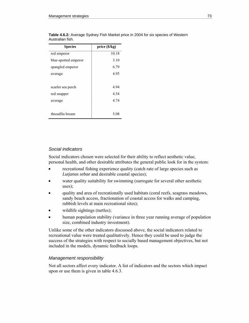
Management strategies 73
Table 4.6.2: Average Sydney Fish Market price in 2004 for six species of Western Australian fish.
Species price ($/kg)
red emperor 10.18
blue-spotted emperor 3.10
spangled emperor 6.79
average 4.95
scarlet sea perch 4.94
red snapper 4.54
average 4.74
threadfin bream 5.08
Social indicators Social indicators chosen were selected for their ability to reflect aesthetic value, personal health, and other desirable attributes the general public look for in the system: • recreational fishing experience quality (catch rate of large species such as
Lutjanus sebae and desirable coastal species); • water quality suitability for swimming (surrogate for several other aesthetic
uses); • quality and area of recreationally used habitats (coral reefs, seagrass meadows,
sandy beach access, fractionation of coastal access for walks and camping, rubbish levels at main recreational sites);
• wildlife sightings (turtles); • human population stability (variance in three year running average of population
size, combined industry investment).
Unlike some of the other indicators discussed above, the social indicators related to recreational value were treated qualitatively. Hence they could be used to judge the success of the strategies with respect to socially based management objectives, but not included in the models, dynamic feedback loops.
Management responsibility Not all sectors affect every indicator. A list of indicators and the sectors which impact upon or use them is given in table 4.6.3.

74
Table 4.6.3: List of indicators and relevant sectors that may impact upon or use them.
Indicator Sectors
Regional habitat diversity All sectors
Water quality in selected zones - offshore Oil and gas production
Water quality in selected zones - inshore Coastal development
Sediment contamination - offshore Oil and gas production
Sediment contamination - inshore Coastal development
Population status of K-selected indicator species
All sectors
Status of expected sensitive or vulnerable habitats
Conservation, fisheries (commercial), coastal development
Primary productivity Oil and gas production, coastal development
Recreational values: recreational fishing experience
Fisheries, (commercial and recreational), conservation
Recreational values: water quality suitability for swimming
Coastal development
Recreational values: quality and area of recreationally used habitats
Coastal development, conservation
Recreational values: observing wildlife Conservation, fisheries (commercial), coastal development
Return (gross revenue) on investment by sector
Relevant sector
Value of production by sector* Relevant sector and overall
Employment level* All sectors
Human population stability* All sectors
Flow of government royalties, combined gross production for all sectors*
All sectors
Per capita gross income* All sectors
* Indices that were not necessarily dynamic in all sectors.
Conclusion 75
5. CONCLUSION
This report has documented the model specifications, development scenarios and management strategies that constitute the three dimensions of an MSE analysis for the North West Shelf. A technical description of the MSE model can be found in the companion report of Gray et al. (2006), while the results of the analysis are reported in Little et al. (2006).
The three model specifications spanned a range of model structures representing both biophysical processes and human impacts. Model structures and parameter values were identified that best matched available historical data (within the 80% confidence intervals). Three of these combinations were then selected for detailed analysis based respectively on an optimistic, a pessimistic and an intermediate interpretation of the system’s productivity and resilience to human impacts.
The three development scenarios aimed to account for uncertainty in the future level of industrial activity in the North West Shelf region. The first development scenario represented recent (i.e. 2002) levels of infrastructure, residential and industrial development and environmental protection. The second development scenario represented the planned development over the next five years with no subsequent development, while the third allowed for a repeated cycle of development of the type planned for the next five years after a further five years. Each scenario included developments in each of the four industry sectors: oil and gas, coastal development, fishing, and conservation.
The three management strategies chosen for evaluation focused on the same four sectors and were closely aligned to existing sector-by-sector legislative requirements. The first management strategy broadly represented the combination of sectoral management strategies in place in 2002. The second management strategy included potential modifications to existing sectoral strategies that might allow some management objectives to be met more effectively, while the third was a set of co-ordinated sectoral strategies, with shared monitoring and the potential for integrated multi-sectoral management responses.
The fourth element of the specification was a set of indicators. A set of the potentially most informative indicators was selected based on previous experience and applications. They were intended to be comprehensive and the final list included indicators relating to environmental, ecological, fisheries, economic and social values.
This report has demonstrated the magnitude and complexity of the task of developing models of ecosystem dynamics, human uses and management responses needed to comprehensively address the issue of managing multiple-uses across a large marine region. Placing these models within an MSE framework has added further complexity, but is seen as an essential step in incorporating the large inherent uncertainties associated with the dynamics of the system. While many improvements can be made, with respect to both specific process models and the broader framework, the study has successfully demonstrated the feasibility of the multiple-use MSE approach within a regional context.

76
REFERENCES
Aberg, P., (1992). Size-based demography of the seaweed Ascophyllum-Nodosum in stochastic environments. Ecology, 73, 1488-1501.
Allen, G.R. & Swainston, R., (1988). The Marine Fishes of North-Western Australia. Western Australian Museum, 210 pp.
Althaus, F., He, X., Sainsbury, K. J., Stanley, C., Campbell, R.A., and Woolley, K.L., in prep a. Epibenthic habitat types and their associations on the Northwest Shelf of Australia described from photographic observations.
Althaus, F., He, X., Woolley, K. L., and Sainsbury, K. J., in prep b. The structure of the demersal fish communities from the Northwest Shelf of Australia.
Andow, D.A., and A.R. Ives. (2002). Monitoring and adaptive resistance management. Ecological Applications 12: 1378-1390. ANZECC & ARMCANZ (2000) Australian and New Zealand guidelines for fresh and marine water quality. National Water Quality Management Strategy No 4, Australian and New Zealand Environment and Conservation Council and Agricultural and Resource Management Council of Australia and New Zealand, Canberra, ACT.
Also available at HTUhttp://www.deh.gov.au/water/quality/nwqms/index.html UTH
Augustin, D., Galzin, R., Legendre, P. and Salvat, B., (1997). Interannual variability of the Tiahura barrier reef communities (Moorea Island, French Polynesia). Oceanologica Acta, 20, 743-756.
Australian Bureau of Statistics. (2001). Retrieved from HTUhttp://www.abs.gov.au UTH
Australian State of the Environment Committee, (2001). Australia State of the Environment 2001, Independent Report to the Commonwealth Minister for the Environment and Heritage, CSIRO Publishing on behalf of the Department of the Environment and Heritage, Canberra.
Barnes, R.D., (1987). Invertebrate Zoology. Saunders College Publishing, Fort Worth, USA. 893pp.
Bell, J.J., (2002). Regeneration rates of a sublittoral demosponge. J. Mar. Biol. Assoc. U. K., 82, 169-170.
Biber, P.D., Harwell, M.A., Cropper, W.P., (2004). Modeling the dynamics of three functional groups of macroalgae in tropical seagrass habitats. Ecol. Model., 175, 25-54.
Bowman Bishaw Gorham, (1995). A Natural Resource Atlas for the North West Shelf, pp. 91–111.
Bridgewater, P.B. and Cresswell, I.D., (1999). Biogeography of mangrove and saltmarsh vegetation: implications for conservation and management in Australia. Mangroves and Salt Marshes, 3, 117-125.
Bruce, B. D., Condie, S. A., and Sutton, C. A., (2001). Larval distribution of blue grenadier (Macruronus novaezelandiae Hector) in south-eastern Australia: further evidence for a second spawning area. Mar. Freshwat. Res., 52, 603-610.

References 77
Buchan, S.J. & Stroud, S.A., (1993). Review of Oceanography of North West Shelf and Timor Sea Regions Pertaining to the Environmental Impact of the Offshore Oil and Gas Industry. Steedman Science & Engineering Report no. R644, Steedman Science and Engineering, Jolimont, WA.
Bulman, C. (2006). Trophic webs and modelling of Australia’s North West Shelf. NWSJEMS Technical Report No 9. CSIRO Marine and Atmopheric Research.
Bureau of Meteorology, Retrieved May 2001 from HTUhttp://www.bom.gov.au/UTH
Cambridge, M.L., Bastyan, G.R., and Walker, D.I., (2002). Recovery of Posidonia meadows in oyster harbour, southwestern Australia. Bull. Mar. Sci., 71, 1279-1289.
Campbell, M.L., (2003). Recruitment and colonisation of vegetative fragments of Posidonia australis and Posidonia coriacea. Aquatic Botany, 76, 175-184.
Carignan, V. and Villard, M.A., (2002). Selecting indicator species to monitor ecological integrity: A review. Environmental Monitoring and Assessment. 78, 45-61.
Carr, B. and Livesey, N., (1996). Pilbara Mangrove Study: Volume 1-Final Report to the Heritage Council of Western Australia MAFRA 96/9 (NEDP).
Chaloupka, M., (2002a). Phase 1 - Assessment of the sustainability of Queensland Parks and Wildlife Service sea turtle data for use in models of the population dynamics of the southern Great Barrier Reef green turtle stock. Research Publication No. 74, Great Barrier Reef Marine Park Authority, Townsville, Queensland, Australia. 49pp.
Chaloupka, M. (2002b). Stochastic simulation modelling of southern Great Barrier Reef green turtle population dynamics. Ecol. Modl. 148, 79-109.
Chaloupka, M., (2003). Stochastic simulation modelling of loggerhead sea turtle population dynamics given exposed to competing mortality risks in the western south Pacific region. In: Bolten, A.B. and Witherington, B.E. (Eds.), Loggerhead sea turtles. Smithsonian Books, Washington, DC, pp.274-294.
Chalpouka, M. and Musick, J.A. (1997). Age, growth and population dynamics. In: Lutz, P.J. and Musick, J.A. (Eds.), The biology of sea turtles. CRC Marine Science, CRC Press Inc, Boca Raton. pp.233-276.
Cheshire, A. and Miller, D., (1996). The potential impact of beach sand replenishment dredging on the Adelaide northern metropolitan beaches: A report to the coast protection branch, Department of Environment and Natural Resources. University of Adelaide, Adelaide, South Australia. 41pp.
Colman, J.G. and West, N.F., (2000). An investigation of benthic sediment characteristics in the vicinity of the Cossack Pioneer FPSO, North West Shelf. APPEA Journal 2000, 667-681.
Commonwealth of Australia (1992). Intergovernmental Agreement on the Environment. AGPS, Canberra.
Commonwealth of Australia (1992). The national strategy for Ecologically Sustainable Development. AGPS, Canberra.
Commonwealth of Australia (1967) Petroleum (Submerged Lands) Act 1967.
78
Condie, S.A., Andrewartha, J., Mansbridge, J., and Waring, J. (2006) Modelling Circulation and Connectivity on Australia’s North West Shelf. NWSJEMS Technical Report No.6. CSIRO Marine and Atmospheric Research.
Condie, S., Fandry, C., McDonald, D., Parslow, J. and Sainsbury, K., (2003). Linking ocean models to coastal management on Australia’s North West Shelf. EOS, Transactions American Geophysical Union, 84, 49-53.
Condie, S. A., Loneragan, N. R., and Die, D. J., (1999). Modelling the recruitment of tiger prawns (Penaeus esculentus and P. semisulcatus) to nursery grounds in the Gulf of Carpentaria, northern Australia: implications for assessing stock-recruitment relationships. Mar. Ecol. Prog. Ser., 178, 55-68.
Creed, J.C., Kain, J.M. and Norton, T.A., (1998). An experimental evaluation of density and plant size in two large brown seaweeds. J. Phycol., 34, 39-52.
Clayton, M.n. and King, R.J. (eds), (1990). Biology of marine plants. Longman Cheshire: Melbourne. 50pp.
DEH 2004. Assessment of the Onslow and Nickol Bay Prawn Managed Fisheries. Department of the Environment and Heritage. November, 2004.
HTUhttp://www.deh.gov.au/coasts/fisheries/wa/onslow/index.htmlUTH
Department of Fisheries, Western Australia, (2002). Application to Environment Australia regarding the Exmouth Gulf Prawn Fishery: Against the Guidelines of the Ecologically Sustainable Management of Fisheries, For Continued Listing on Section 303DB of the Environmental Protection and Biodiversity Conservation Act 1999. Western Australian Government, Perth. 143pp.
Dritschel, D.G., (1989). Contour Dynamics and Contour Surgery: Numerical algorithms for extended high-resolution modelling of vortex dynamics in two-dimensional, inviscid, incompressible flows. Comp. Phys. Rep., 10, 77pp.
Eckert, S.A., (2002) Swim speed and movement patterns of gravid leatherback sea turtles (Dermochelys coriacea) at St Croix, US Virgin Islands. The Journal of Experimental Biology, 205: 3689-3697.
Environment Australia, (2000). National Marine Turtle Recovery Plan. DEH: Canberra. Also available at http://www.deh.gov.au/coasts/species/turtles/
Fandry, C.B., Revill, A.T., Wenziker, K.J., McAlpine, K.W., Apte, S.C., Masini, R.J., and Hillman, K. (2006). Contaminants on Australia’s North West Shelf: sources, impacts, pathways and effects. NWSJEMS Technical Report No. 13. CSIRO Marine and Atmospheric Research.
Fletcher, W., Chesson, J., Fisher, M., Sainsbury, K. J., Hundloe, T., Smith, A. D. M., and Whitworth, B., (2002). National ESD reporting framework for Australian fisheries: the 'how to' guide for wild capture fisheries. Version 1.01 ed. 120pp. FRDC Project, 2000/145. W.A. Dept. of Fisheries//FRDC, Canberra.
FISHBASE (2005). Froese, R. and Pauly, D. (Eds.). FishBase. World Wide Web electronic publication. www.fishbase.org, version (09/2005).
Frost, B.W., (1987). Grazing control of phytoplankton stock in the open subarctic Pacific Ocean: a model assessing the role of mesozooplankton, particularly the large calanoid copepods Neocalanus spp. Mar. Ecol. Prog. Ser., 39, 49-68.

References 79
Frost, T. M., Carpenter, S. R., and Kratz, T. K., (1992). Choosing ecological indicators: effects of taxonomic aggregation on sensitivity to stress and natural variability. In: McKenzie, D.H., Hyatt, D. E., and McDonald, V. J. (Eds.), Ecological indicators. Elsevier Applied Science Publishers, Essex, England. pp.215-227.
Fulton, E.A., Hatfield, B., Althaus, F., and Sainsbury, K. (2006). Benthic habitat dynamics and models on Australia’s North West Shelf. NWSJEMS Technical Report No. 11. CSIRO Marine and Atmospheric Research.
Fulton, E.A., Smith, A.D.M., Webb, H. and Slater, J. (2004) Ecological indicators for the impacts of fishing on non-target species, communities and ecosystems: Review of potential indicators. AFMA final research report (R99/1546).
Fulton E., Kault, D., Mapstone B. and Sheaves, M., (1999). Spawning season influences on commercial catch rates: computer simulations and Plectropomus leopardus, a case in point. Canadian Journal of Fisheries and Aquatic Sciences 56: 1096 – 1108.
Garrabou, J. and Zabala, M., (2001). Growth dynamics in four Mediterranean demosponges. Estuar. Coast. Shelf Sci., 52, 293-303.
Geoscience Australia (2000) – GEODATA TOPO 250K Series 1.
Geoscience Australia (1998) – Bathymetric 30 second grid of the Australian Region.
Gordon, D. (2006) Summary of International Conventions, Commonwealth and State legislation and other instruments affecting marine resource allocation use, conservation and environmental protection on the North West shelf of Australia. NWSJEMS Technical Report No. 3. CSIRO Marine and Atmospheric Reaserach.
Government of Western Australia (1997) Acts Ammendment (Marine Reserves) Act 1997.
Government of Western Australia (1994) Conservation and lands managent Act 1994.
Government of Western Australia (1994) Fish Resources Management Act (FRMA) 1994.
Government of Western Australia (1986-93) Environmental Protectioon Act 1986-93 (or as amended).
Government of Western Australia (1985) Western Australain planning Commission Act 1985.
Government of Western Australia (1982) Petroleum (Submerged Lands) Act 1982.
Government of Western Australia (1982) Western Australia Marine Act 1982.
Government of Western Australia (1981) Prevention of a Collistion at Sea Regulations 1983.
Government of Western Australia (1981) Marine and Harbours Act 1981.
Government of Western Australia (1967) Shipping and Pilotage Act 1967.
Government of Western Australia (1950) Wildlife Conservation Act 1950.
Gray, R., Fulton, E.A., Little, L.R. and Scott, R. (2006). Ecosystem model specification within an agent based framework. NWSJEMS Technical Report No. 16. CSIRO Marine and Atmospheric Research.
80
Grimbly, M., (2005) HTUhttp://wwwistp.murdoch.edu.au/Susty_case_studies/Pilbara/economic/Fisheries_Aquaculture.htm# UTH Murdoch University, Western Australia.
Grove, S.J., Turton, S.M., and Siegenthaler, D.T., (2000). Mosaics of canopy openness induced by tropical cyclones in lowland rain forests with contrasting management histories in northeastern Australia. J. Trop. Ecol., 16, 883-894.
Hall, S.J. (1999). The effects of fishing on marine ecosystems and communities. Blackwell Science Ltd, Oxford.
Harrison, F.W. and Cowden, R.R. (1976). Aspects of sponge biology. Academic Press, New York.
Hashmi, M.I., Mustafa, S., and Tariq, S.A., (2002). Heavy metal concentrations in water and tiger prawn (Penaeus monodon) from grow-out farms in Sabah, North Borneo. Food Chem., 79, 151-156.
Hatfield, B., Thomas, L., Scott, R., (2006). Management strategy evaluations for multiple use management of Australia’s North West Shelf: visualisation software and user guide. NWSJEMS Technical Report No. 17. CSIRO Marine and Atmospheric Research.
Henry, G.W. and Lyle, JM. (Eds.), (2003). The national recreational and indigenous fishing survey. FRDC Final report 99/158. NSW Fisheries, Cronulla.
Herzfeld, M., Parslow, J., Sakov, P., and Andrewartha, J.R. (2006). Biogeochemical modelling on Australia’s North West Shelf. NWSJEMS Technical Report No. 8. CSIRO Marine and Atmospheric Research.
Herzfeld, M., Waring, J., Parslow, J., Margvelashvili, N., Sakov, P., and Andrewartha, J. (2002). MECO, Model of Estuarine and Coastal Oceans, V4.0, Scientific Manual. CSIRO Marine Research.
Hill, B. J., (1985). Effect of temperature on duration of emergence speed of movement, and catchability of the prawn Penaeus esculentus. In: Rothlisberg, P C, Hill, B J and Staples, D J (Eds.) 2nd Australian National Prawn Seminar, Kooralbyn, Qld., October 1984. Cleveland, Qld., National Prawn Seminar 2, pp. 77-83 18 refs.
Jones, H.A., (1973). Marine geology of the North-West Australia continental shelf. Bur. Miner. Resour. Geol. Geophys. Bull., 136, 19pp.
Kabanova, Y.G., (1968). Primary production of the northern part of the Indian Ocean. Oceanography, 8, 214-225.
Kailola, P.J., Williams, M.J., Stewart, P.C., Reichelt, R.E., McNee, A., and Grieve, C. (1993). Australian fisheries resources. BRS and FRDC, Canberra.
Kalnay, E., Kanamitsu, M., Kistler, R., Collins, W., Deaven, D., Gandin, L., Iredell, M., Saha, S., White, G., Woollen, J., Zhu, Y., Chelliah, M., Ebisuzaki, W., Higgins, W., Janowiak, J., Mo, K.C., Ropelewski, C., Wang, J., Leetmaa, A., Reynolds, R., Jenne, R., and Joseph, D., (1996). The NCEP/NCAR 40-year reanalysis project. Bull. Amer. Meteor. Soc., 77, 437-471.
Kathiresan, K. and Bingham., B.L., (2001). Biology of Mangroves and Mangrove Ecosystems. Adv. Mar. Biol., 40, 81-251.
Last, P.R. and Stevens, J.D., (1994). Sharks and rays of Australia. FRDC and CSIRO.

References 81
Levins, R., (1969). Some demographic and genetic consequences of environmental heterogeneity for biological control. Bull. Entomol. Soc. Amer., 15, 237-240.
Limpus, C.J., Eggler, P. and Miller, J.D., (1994). The green turtle, Chelonia mydas, in Queensland: population structure in a warm temperate feeding area. Memoirs Queensland Museum., 35, 139-154.
Limpus, C.J., Fleay, A. and Guinea, M., (1984). Sea turtles of the Capricornia section, Great Barrier Reef. In: Ward, W.T., and Saenger, P. (Eds.), The Capricornia section of the Great Barrier Reef Marine Park: past, present and future. Royal Society of Queensland and Australian Coral Reef Society, Brisbane. pp.61-78.
Limpus, C.J., and Reed, P., (1985). The green turtle, Chelonia mydas, in Queensland: a preliminary description of the population structure in a coral reef feeding ground. In: Grigg, G., Shine, R., and Ehmann, H. (Eds.), Biology of Australasian Frogs and Reptiles. Royal Zoological Society of New South Wales, Sydney. pp.47-52.
Little, L.R., Fulton, E.A., Gray, R., Hayes, D., Lyne, V., Scott, R., Sainsbury, K and McDonald, D. (2006). Management Strategy Evaluation results and discussion for Australia’s North West Shelf. NWSJEMS Technical Report No. 14. CSIRO Marine and Atmospheric Research.
Lyne, V.D., Gray, R.C., Sainsbury, K.J., and Scott, R., (1994). Research on Jarosite Dumping at Sea. Volume 5: Integrated Biophysical Model Investigations. A Program of Research on Jarosite Dumping at Sea by Pasminco Metals-EZ. Report Commissioned by the Commonwealth Department of the Arts, Sport, the Environment, Tourism and Territories. December 1994. 169pp.
Marine Parks and Reserves Selection Working Group (1994). A representative marine reserve system for Western Australia. Report of the Marine Parks and Reserves Selection Working Group. Department of Conservation and Land Management, Perth.
Marsh, H., Corkeron, P., Preen, T., and Pantus, F. (2004), Aerial Survey of Marine Wildlife in the Gulf of Carpentaria. As of National Heritage Trust, Marine Species Protection Program Completed Projects, at http://www.nht.gov.au/nht1/programs/mspp/gulf.html
Marsh, H., and Saalfield, W.K., (1989). Aerial surveys of sea turtles in the northern Great Barrier Reef Marine Park. Australian Wildlife Research, 16, 239-249.
McCook, L.J., Klumpp, D.W., and McKinnon, A.D., (1995). Seagrass communities in Exmouth Gulf, Western Australia: A preliminary survey. J. Roy. Soc. West. Aust., 78, 81-87.
McGuinness, K.A., (1997). Dispersal, establishment and survival of Ceriops tagal propagules in a north Australian mangrove forest. Oecologia, 109, 80-87.
McLoughlin, R. J., and Young, P. C., (1985). Sedimentary provinces of the fishing grounds of the North West shelf of Australia: grain size frequency analysis of surficial sediments. Aust. J. Mar. Freshw. Res., 36, 671-681.
Milton, D. A., Die, D. J., Tenakanai, C., and Swales, S. (1998). Selectivity for barramundi (Lates calcarifer) in the Fly River, Papua New Guinea: implications for managing gill-net fisheries on protandrous fishes. Marine and Freshwater Research, 49 (6): 499-506.

82
Meyer, D.L., Fonseca, M.S., Murphey, P.L., McMichael, R.H., Byerly, M.M., LaCroix, M.W., Whitfield, P.E. and Thayer, G.W., (1999). Effects of live-bait shrimp trawling on seagrass beds and fish bycatch in Tampa Bay, Florida. Fishery Bulletin, 97, 193-199.
Moran, M.J. and Stephenson, P.C., (2000). Effects of otter trawling on macrobenthos and management of demersal scalefish fisheries on the continental shelf of north-western Australia. ICES J. Mar. Sci., 57, 510-516.
Moran, M.J., and Jenke, J. (1990). Effects of fish trap mesh size on species and size selectivity in the Australian North West shelf trap fishery. Western Australian Marine Research Laboratories.
Motoda, S., Kawamusra, T. and Taniguchi, A., (1978). Differences in productivities between the Great Australian Bight and the Gulf of Carpentaria, Australia, in summer. TMarine Biology (Berl) T, 46, 93-99.
Murray, A. and Parslow, J., (1997). Port Phillip Bay Integrated Model: Final Report. Port Phillip Bay Environmental Study, Technical Report 44. CSIRO, Canberra. 201pp.
Newell, R.C., Seiderer, L.J., Simpson, N.M. and Robinson, J.E., (2004). Impacts of marine aggregate dredging on benthic macrofauna off the south coast of the United Kingdom. J. Coast. Res., 20, 115-125.
Paling, E., (1996). Mangrove Processes in the Port Headland Harbour and Surrounds: Tidal creek erosion & mangrove health from September 1993 to March 1995 MAFRA 96/8 (BHP).
Pilbara Fish Trawl Fishery (Interim) Management Plan 1997, Western Australian Department of Fisheries.
Pilbara Trap Management Plan 1992 (WA) Western Australian Department of Fisheries.
Preen, A.R., Long, W.J.L., Coles, R.G., (1995). Flood and cyclone related loss, and partial recovery, of more than 1000 kmP
2P of seagrass in Hervey-Bay, Queensland,
Australia. Aquatic Botany, 52, 3-17.
Prince, R.I.T. (2001). Aerial survey of the distribution and abundance of dugongs and associated macroverterate fauna – pilbara coastal and offshore region, WA: Completion report. Environment Australia. 39pp.
Revill, A. (2002). Fate and Pathways of Key Contaminants on the North West Shelf. North West Shelf Joint Environmental Management Study: Task 3.2. CSIRO Marine Research.
Roberts, R.D., Gregory, M.R. and Foster, B.A., (1998). Developing an efficient macrofauna monitoring index from an impact study - A dredge spoil example. Mar. Poll. Bull., 36, 231-235.
Robertson, AI., and Alongi, D.M., (Eds.), (1992). Tropical mangrove ecosystems. Coastal and Estuarine Studies 41. American Geophysical Union, Washington DC. 329pp.
Sainsbury, K.J., (1987). Assessment and management of the demersal fishery on the continental shelf of northwestern Australia. In: Polovina, J. J. and Ralston, S. (Eds.), Tropical snappers and groupers: biology and fisheries management. Chapter 10. Ocean Resources and Marine Policy Series. Westview Press, Boulder, Colorado. pp.465-502.
References 83
Sainsbury, K. J., (1988). The ecological basis of multispecies fisheries, and management of a demersal fishery in tropical Australia. In: Gulland, J. A. (Ed.), Fish population dynamics, (2nd ed.). John Wiley & Sons Ltd. pp.349-382.
Sainsbury, K. J., (1991). Application of an experimental approach to management of a tropical multispecies fishery with highly uncertain dynamics. ICES Mar. Sci. Symp., 193, 301-320.
Sainsbury, K.J., Campbell, R.A., Lindholm, R., and Whitelaw, A.W., (1997). Experimental management of an Australian multispecies fishery: examining the possibility of trawl-induced habitat modification. In: Pikitch, E.K., Huppert, D.D., and Sissenwine, M.P. (Eds.). Global Trends: Fisheries Management. American Fisheries Society, Bethesda, Maryland. pp.107-112.
Sainsbury, K. J., Punt, A. E., and Smith, A. D. M. (2000). Design of operational management strategies for achieving fishery ecosystem objectives. ICES Journal of Marine Science, 57 (3): 731-741.
Semeniuk, V., (1994). Predicting the effect of sea-level rise on mangroves in northwestern Australia. J. Coast. Res., 10, 1050-1076.
Semeniuk, V. and Semeniuk, C., (1995). Study of the impacts of Pilbara coastal developments on arid zone mangroves – stage 3: assessment of impacts of miscellaneous industries and infrastructures. Department of Resource Development, Perth Western Australia. 23pp.
Semeniuk, V. and Semeniuk, C., (1997). The Mangrove Database, Western Australia. Unpublished report submitted to the Department of Environment, Canberra. Sit V. and Taylor B. J. R. (1998). Statistical Methods for Adaptive Management Studies. B.C. Ministry of Forests, Forestry Division Services Branch, Victoria, B.C.
Solidoro, C., Pecenik, G., Pastres, R., Franco, D. and Dejak, C., (1997). Modelling macroalgae (Ulva rigida) in the Venice lagoon: Model structure identification and first parameters estimation. Ecol. Model., 94, 191-206.
Stephenson, P. and Chidlow, J. (2003). By-catch in the Pilbara Trawl Fishery. Report by Department of Fisheries, Western Australia.
Taylor B. and Dichmont C. (2001). Northern Prawn Fishery 2000. Northern Prawn Fishery Assessment Group (NPFAG) Report. 79pp.
Tett P., (1990). The photic zone. In: Herring, P.J., Cambell, A.K., Whitfield, M. and Maddock, L. (Eds.), Light and Life in the Sea. Cambridge. pp.59-87.
Tilman, D., and P. Kareiva, (Eds.), (1997). Spatial ecology: the role of space in population dynamics and interspecific interactions. Princeton University Press, Princeton, New Jersey, USA.
Tranter, D.J., (1962). Zooplankton abundance in Australian waters. Aust. J. Mar. Freshw. Res., 13, 106-142.
van Tussenbroek, B.I., (2002). Static life-table analysis and demography of the foliar shoots of the tropical seagrass Thalassia testudinum. Bull. Mar. Sci., 71, 1247-1256.
WA Fisheries (2002). State of the Fisheries Report 2001-2002. Department of Fisheries Western Australia, Perth.

84
Walker, S.J., (1999). Coupled hydrodynamic and transport models of Port Phillip Bay, a semi-enclosed bay in south-eastern Australia. Mar. Freshwat. Res., 50, 469-481.
Walker, D.I. and Prince, R.I.T., (1987). Distribution and biogeography of seagrass species on the northwest coast of Australia. Aquatic Botany, 29, 19-32.
TWalter, M.T., M.F. Walter, E.S. Brooks, T.S. Steenhuis, J. Boll, K.R. Weiler. (2000). Hydrologically sensitive areas: Variable Source Area hydrology implications for water quality risk assessment. J. Soil and Water Conservation 55(3):277-284.
Whitfield, A.K., and Elliott, M., (2002). Fishes as indicators of environmental and ecological changes within estuaries – a review of progress and some suggestions for the future. J. Fish Biol., 61(Suppl. A), 229-250. T
Wyrtki, K. (1961). Scientific results of marine investigation of the South China Sea and Gulf of Thailand 1959 – 1961. NAGA Reports Vol 2. 195pp.
Zann, L.P. (1995). Our Sea, Our Future, Major Findings of the State of the Marine Environment Report for Australia, Great Barrier Reef Marine Park Authority, Ocean Rescue 2000, Department of the Environment, Sport and Territories, Canberra.
Appendix A: List of InVitro input data sets 85
APPENDIX A: LIST OF INVITRO INPUT DATA SETS
abbrev_pilb_traps.xy.pt
abbrev_pilbara-prawns.xy.pt
abbrev_pipelines_new.xy.pt
abbrev_wells.xy.pt
AirlieIsA_Oil.ts
irlieIsA_ProducedFormationWater.ts
BananaprawnNODAT.SAD
BananaPrawnSpatialCatch.his
Burrup-bbox.ll.pt
bycatch.ll.pt
bycatch.xy.pt
C-Lambert-in.pt
C-Lambert-out.pt
condensate-prod.ts
condensate-prod-1p.ts
condensate-prod-2p.ts
Cossack_Oil.ts
Cossack_ProducedFormationWater.ts
currents.data
Cyclones.data
D_003_Prawn.BB
Dampier-in.pt
Dampier-out.pt
Dampier-Overflow-in.pt
Dampier-Overflow-out.pt
Dampier-pop.ts
Dampier-pop-1p.ts
Dampier-pop-2p.ts
Dampier-prod.ts
Dampier-prod-1p.ts
Dampier-prod-2p.ts
deep.xy.pt
Disasters.data
Dredge.data
Dredge_enhanced_1p.data
Dredge_enhanced_2p.data
East-intercourse-island-in.pt
East-intercourse-island-out.pt
effort.his
effortTrap.his
Exmouth-pop.ts
Exmouth-pop-1p.ts
Exmouth-pop-2p.ts
Exmouth-prawn.xy.pt
Exmouth-prod.ts
Exmouth-prod-1p.ts
Exmouth-prod-2p.ts
ExtraDisasters.data
F_015_Prawn.BB
F_024_Prawn.BB
F_358_Prawn.BB
F_424_Prawn.BB
F_447_Prawn.BB
F_454_Prawn.BB
F_465_Prawn.BB
F_474_Prawn.BB
F_477_Prawn.BB
F_479_Prawn.BB
F_501_Prawn.BB
F_543_Prawn.BB
F_550_Prawn.BB
F_556_Prawn.BB
F_561_Prawn.BB
F_630_Prawn.BB
F_814_Prawn.BB
F_824_Prawn.BB
file.txt
G_142_Prawn.BB
86
G_223_Prawn.BB
G_350_Prawn.BB
gas-net.ts
gas-prod.ts
gas-prod-1p.ts
gas-prod-2p.ts
GoodwynA_Oil.ts
GoodwynA_ProducedFormationWater.ts
Griffin_Oil.ts
Griffin_ProducedFormationWater.ts
HammersleyWTP_Copper.ts
HammersleyWTP_Copper_1p.ts
HammersleyWTP_Copper_2p.ts
HammersleyWTP_Copper1p.ts
HammersleyWTP_Copper2p.ts
HammersleyWTP_flow.ts
HammersleyWTP_flow-1p.ts
HammersleyWTP_flow1p.ts
HammersleyWTP_flow-2p.ts
HammersleyWTP_flow2p.ts
HarrietA_Bitterns.ts
HarrietA_Lead.ts
HarrietA_Oil.ts
HarrietA_ProducedFormationWater.ts
HarrietB_ProducedFormationWater.ts
HarrietC_Oil.ts
HarrietC_ProducedFormationWater.ts
HeavyExtraDisasters.data
KingprawnNODAT.SAD
KingPrawnSpatialCatch.his
leth.his
lethTrap.his
llut.his
llutTrap.his
lsebae.his
LSebaeNODAT.SAD
LSebaeNODATB.SAD
lsebaeTrap.his
M_135_Prawn.BB
macrophytegrids.ll.pt
mangrovegrids.ll.pt
map.rc
merged_xy.pfm
MermaidSound_Cadmium.ts
MermaidSound_Cadmium-1p.ts
MermaidSound_Cadmium1p.ts
MermaidSound_Cadmium-2p.ts
MermaidSound_Cadmium2p.ts
MermaidSound_Copper.ts
MermaidSound_Copper-1p.ts
MermaidSound_Copper1p.ts
MermaidSound_Copper-2p.ts
MermaidSound_Copper2p.ts
MermaidSound_flow.ts
MermaidSound_flow-1p.ts
MermaidSound_flow1p.ts
MermaidSound_flow-2p.ts
MermaidSound_flow2p.ts
MermaidSound_Lead.ts
MermaidSound_Lead-1p.ts
MermaidSound_Lead1p.ts
MermaidSound_Lead-2p.ts
MermaidSound_Lead2p.ts
MermaidSound_Oil.ts
MermaidSound_Oil-1p.ts
MermaidSound_Oil1p.ts
MermaidSound_Oil-2p.ts
MermaidSound_Oil2p.ts
MermaidSound_PetroleumHydrocarbons.ts
MermaidSound_PetroleumHydrocarbons-1p.ts
MermaidSound_PetroleumHydrocarbons1p.ts
MermaidSound_PetroleumHydrocarbons-2p.ts
MermaidSound_PetroleumHydrocarbons2p.ts
MermaidSound_Sulphate.ts
MermaidSound_Sulphate-1p.ts
MermaidSound_Sulphate1p.ts
MermaidSound_Sulphate-2p.ts
MermaidSound_Sulphate2p.ts
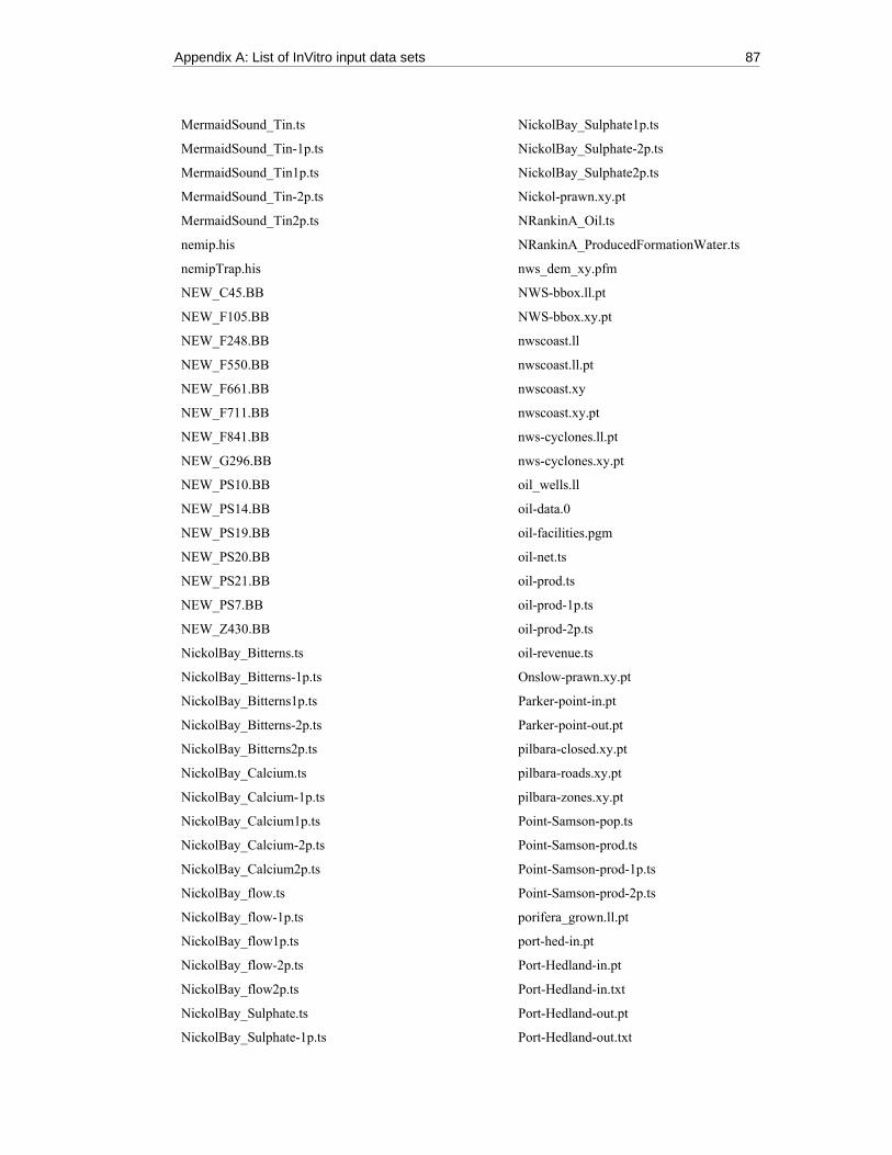
Appendix A: List of InVitro input data sets 87
MermaidSound_Tin.ts
MermaidSound_Tin-1p.ts
MermaidSound_Tin1p.ts
MermaidSound_Tin-2p.ts
MermaidSound_Tin2p.ts
nemip.his
nemipTrap.his
NEW_C45.BB
NEW_F105.BB
NEW_F248.BB
NEW_F550.BB
NEW_F661.BB
NEW_F711.BB
NEW_F841.BB
NEW_G296.BB
NEW_PS10.BB
NEW_PS14.BB
NEW_PS19.BB
NEW_PS20.BB
NEW_PS21.BB
NEW_PS7.BB
NEW_Z430.BB
NickolBay_Bitterns.ts
NickolBay_Bitterns-1p.ts
NickolBay_Bitterns1p.ts
NickolBay_Bitterns-2p.ts
NickolBay_Bitterns2p.ts
NickolBay_Calcium.ts
NickolBay_Calcium-1p.ts
NickolBay_Calcium1p.ts
NickolBay_Calcium-2p.ts
NickolBay_Calcium2p.ts
NickolBay_flow.ts
NickolBay_flow-1p.ts
NickolBay_flow1p.ts
NickolBay_flow-2p.ts
NickolBay_flow2p.ts
NickolBay_Sulphate.ts
NickolBay_Sulphate-1p.ts
NickolBay_Sulphate1p.ts
NickolBay_Sulphate-2p.ts
NickolBay_Sulphate2p.ts
Nickol-prawn.xy.pt
NRankinA_Oil.ts
NRankinA_ProducedFormationWater.ts
nws_dem_xy.pfm
NWS-bbox.ll.pt
NWS-bbox.xy.pt
nwscoast.ll
nwscoast.ll.pt
nwscoast.xy
nwscoast.xy.pt
nws-cyclones.ll.pt
nws-cyclones.xy.pt
oil_wells.ll
oil-data.0
oil-facilities.pgm
oil-net.ts
oil-prod.ts
oil-prod-1p.ts
oil-prod-2p.ts
oil-revenue.ts
Onslow-prawn.xy.pt
Parker-point-in.pt
Parker-point-out.pt
pilbara-closed.xy.pt
pilbara-roads.xy.pt
pilbara-zones.xy.pt
Point-Samson-pop.ts
Point-Samson-prod.ts
Point-Samson-prod-1p.ts
Point-Samson-prod-2p.ts
porifera_grown.ll.pt
port-hed-in.pt
Port-Hedland-in.pt
Port-Hedland-in.txt
Port-Hedland-out.pt
Port-Hedland-out.txt

88
Port-Hedland-Overflow-in.pt
Port-Hedland-Overflow-out.pt
Port-Hedland-pop.ts
Port-Hedland-pop-1p.ts
Port-Hedland-pop-2p.ts
Port-Hedland-prod.ts
Port-Hedland-prod-1p.ts
Port-Hedland-prod-2p.ts
port-hed-out.pt
portLineCossack.pt
portLineCossack.rt
portLineN_Rankin_A.pt
portLineN_Rankin_A.rt
portLineOre.pt
portLineOre.rt
portLineOre2.pt
portLineOre2.rt
portLineOre3.pt
portLineOre3.rt
portLineOre4.rt
portLineRigs.pt
PrawnEffortSpatial.his
PS017_Prawn.BB
PS019_Prawn.BB
PtSamson-in.pt
PtSamson-out.pt
rainfall_60.ts
rigs-cadastre.xy.pt
Salt-prod.pt
saur.his
saurTrap.his
sed381.xy.pt
slut.his
slutTrap.his
Stag_Oil.ts
Stag_ProducedFormationWater.ts
ThevenardIs_Oil.ts
ThevenardIs_ProducedFormationWater.ts
tuv_mh.data
tuv_ml.data
tuv_mn.data
vesNothing.BB
Wandoo_Oil.ts
Wandoo_ProducedFormationWater.ts
wind.data

Appendix B: Selected model parameters 89
APPENDIX B: SELECTED MODEL PARAMETERS
Table B.1: Base case parameters set for continental shelf reef habitat (sponges, soft corals, etc) in North West Shelf benthic habitat model. Those entries marked with an asterisk are transformed in the calculation dependent on size of habitat patches, activity/event footprint and fragmentation index for that cell of the benthic habitat model.
Parameter Value Notes
Small reef habitat
Horizontal growth rate (µBs B) 0.103 estimated
Index of spread for growth (λ) 1.0 Fixed (based on expert knowledge)
Inflexion point for growth (ν) 4.0 Fixed (based on expert knowledge)
Recruitment rate (ξ) 0.05 estimated
Natural mortality rate (κBs B) 0.012 estimated
Index of spread for mortality (θ) 1.0 Fixed (based on expert knowledge)
Inflexion point for mortality (ϕ) 11.0 Fixed (based on expert knowledge)
Vulnerability to trawling 0.09* Fixed (based on Hall (1999))
Vulnerability to dredging 1.0* Fixed (based on Roberts (1998) and Newell et al. (2004)
Vulnerability to cyclones 0.4* Fixed (based on Augustin et al. (1997))
Transition (vertical growth) rate (ω) 0.05 Fixed (based on Harrison & Cowden (1976), Barnes (1987), Garrabou & Zabala (2001) and Bell (2002))
Index of spread for transition (θ) 1.5 Fixed
Inflexion point for transition (ϕ) 9.0 Fixed
Number of age-size classes (χ) 10.0 Fixed (computationally efficient while still capturing the typical span of size and ages for sponges less than 20cm in height, from information in Barnes (1987)).

90
Table B.2: Base-case parameters set for seagrass habitat in North West Shelf benthic habitat model. Those entries marked with an asterisk are transformed in the calculation dependent on size of habitat patches, activity/event footprint and fragmentation index for that cell of the benthic habitat model.
Parameter Value Notes
Horizontal growth rate (µBL B) 0.5 Fixed (based on Cambridge et al. (2002) and Campbell (2003))
Growth coefficient for depth effect (ϖ) 0.1 estimated - simple least squares estimation
Growth coefficient for sediment effect (ζ) 1.0 estimated - simple least squares estimation
Natural mortality rate (κBs B) 0.2 Fixed (based on van Tussenbroek (2002) and Biber et al. (2004))
Vulnerability to trawling 0.8* Fixed (based on Hall (1999) and Meyer et al. (1999))
Vulnerability to dredging 1.0* Fixed (based on Cheshire & Miller (1996))
Vulnerability to cyclones 0.4* Fixed (based on Preen et al. (1995))
Table B.3: Base-case parameters set for macroalgae in North West Shelf benthic habitat model. Those entries marked with an asterisk are transformed in the calculation dependent on size of habitat patches, activity/event footprint and fragmentation index for that cell of the benthic habitat model.
Parameter Value Notes
Horizontal growth rate (µBL B) 0.1 Fixed (based on Creed et al. (1998))
Growth coefficient for depth effect (ϖ) 0.1 estimated - simple least squares estimation
Growth coefficient for sediment effect (ζ) 1.0 estimated - simple least squares estimation
Natural mortality rate (κBs B) 0.2 Fixed (based on Aberg (1992) and Solidoro et al. (1997))
Vulnerability to trawling 0.7* Fixed (based on Hall (1999))
Vulnerability to dredging 1.0* Fixed (based on Roberts (1998) & Newell et al. (2004)
Vulnerability to cyclones 0.3* Fixed (based on Augustin et al. (1997))

Appendix B: Selected model parameters 91
Table B.4: Base-case parameters set for mangroves in North West Shelf benthic habitat model. Those entries marked with an asterisk are transformed in the calculation dependent on size of habitat patches, activity/event footprint and fragmentation index for that cell of the benthic habitat model.
Parameter Value Notes
Small mangroves
Horizontal growth rate (µBs B) 0.01 Fixed (based on Robertson & Alongi (1992))
Index of spread for growth (λ) 0.15 estimated - simple least squares estimation
Inflection point for growth (ν) 1.0 estimated - simple least squares estimation
Recruitment rate (ξ) 0.01 Fixed (based on Robertson & Alongi (1992) and McGuinness (1997))
Natural mortality rate (κBs B) 0.01 Fixed (based on Robertson & Alongi (1992))
Index of spread for mortality (θ)
1.0 estimated - simple least squares estimation
Inflection point for mortality (ϕ)
7.0 estimated - simple least squares estimation
Vulnerability to clearing 1.0* Fixed (based on Semeniuk (1994), Semeniuk & Semeniuk (1995, 1997))
Vulnerability to cyclones 0.7* Fixed (based on Grove et al. (2000) and Kathiresan & Bingham (2001))
Transition (vertical growth) rate (ω)
0.09 Fixed (based on Robertson & Alongi (1992))
Index of spread for transition (θ)
0.8 estimated - simple least squares estimation
Inflection point for transition (ϕ)
12.0 estimated - simple least squares estimation
Number of age-size classes (χ)
10.0 Fixed (computationally efficient while still capturing the typical span of size and ages for mangroves less than 100cm in height, from information in Robertson & Alongi (1992))
Large mangroves
Horizontal growth rate (µBL B) 0.0005 Fixed (based on Robertson & Alongi (1992))
Growth coefficient for depth effect (ϖ)
1.0 estimated - simple least squares estimation
Growth coefficient for sediment effect (ζ)
1.0 estimated - simple least squares estimation
Natural mortality rate (κBs B) 0.001 Fixed (based on Robertson & Alongi (1992))
Vulnerability to clearing 1.0* Fixed (based on Semeniuk (1994), Semeniuk & Semeniuk (1995, 1997))
Vulnerability to cyclones 0.7* Fixed (based on Grove et al. (2000) and Kathiresan & Bingham (2001))

92
Table B.5: Limits of available biomass for the different species groups (based on Bulman, 2006).
Species group min max
Lutjanus sebae 2,500 t 6,500 t
large lutjanids
L. erythropterus, L. malabaricus
1,000 t 16,000 t
lethrinids 6,500 t 220,000 t
small lutjanids
L. vitta
20,000 t 590,000 t
nemipterids 12,000 t 70,000 t
saurids 7,000 t 35 000 t
Table B.6: Stock recruitment parameters for optimistic, base-case and pessimistic model specifications.
Specification
Species group Parameter Optimistic Base case Pessimistic
Lutjanus sebae α 3000 3000 3000
β 1000 5000 9000
Large lutjanids:
L. erythropterus, L. malabaricus
α 30000 30000 30000
β 100 5000 10000
lethrinids α 300000 30000 300000
β 10000 30000 50000
small lutjanids
L. vitta
α 900000 100000 300000
β 100000 10000 90000
nemipterids α 700000 700000 700000
β 70000 90000 100000
saurids α 30000 30000 30000
β 10000 50000 60000
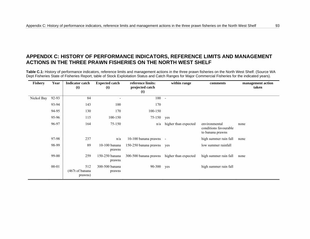
Appendix C: History of performance indicators, reference limits and management actions in the three prawn fisheries on the North West Shelf 93
APPENDIX C: HISTORY OF PERFORMANCE INDICATORS, REFERENCE LIMITS AND MANAGEMENT ACTIONS IN THE THREE PRAWN FISHERIES ON THE NORTH WEST SHELF
Table C.1: History of performance indicators, reference limits and management actions in the three prawn fisheries on the North West Shelf. (Source WA Dept Fisheries State of Fisheries Report, table of Stock Exploitation Status and Catch Ranges for Major Commercial Fisheries for the indicated years).
Fishery Year Indicator catch (t)
Expected catch (t)
reference limits: projected catch
(t)
within range comments management action taken
Nickol Bay 92-93 84 - 100 -
93-94 143 100 170
94-95 130 170 100-150
95-96 115 100-150 75-150 yes
96-97 164 75-150 n/a higher than expected environmental conditions favourable to banana prawns
none
97-98 237 n/a 10-100 banana prawns - high summer rain fall none
98-99 89 10-100 banana prawns
150-250 banana prawns yes low summer rainfall
99-00 259 150-250 banana prawns
300-500 banana prawns higher than expected high summer rain fall none
00-01 512 (467t of banana
prawns)
300-500 banana prawns
90-300 yes high summer rain fall

94
Fishery Year Indicator catch
(t) Expected catch
(t) reference limits: projected catch
(t)
within range comments management action taken
01-02 11 90-300 90-300 lower than expected below acceptable range due to environmental conditions
none
Onslow 92-93 56 - 50
93-94 138 50 120 catch taken from beyond traditional fishing area
94-95 178 120 80-100 higher than expected favourable conditions for tiger prawns
none
95-96 97 80-100 80-100 yes
96-97 94 80-100 n/a yes
97-98 120 n/a 30-265 - high rainfall
98-99 61 30-265 61-132 yes low summer rainfall
99-00 93 61-132 61-132 yes low summer rainfall gave low banana prawn catches
00-01 87 61-132 60-130 yes high summer rainfall gave higher banana prawn catches
01-02 63 60-130 60-130 yes
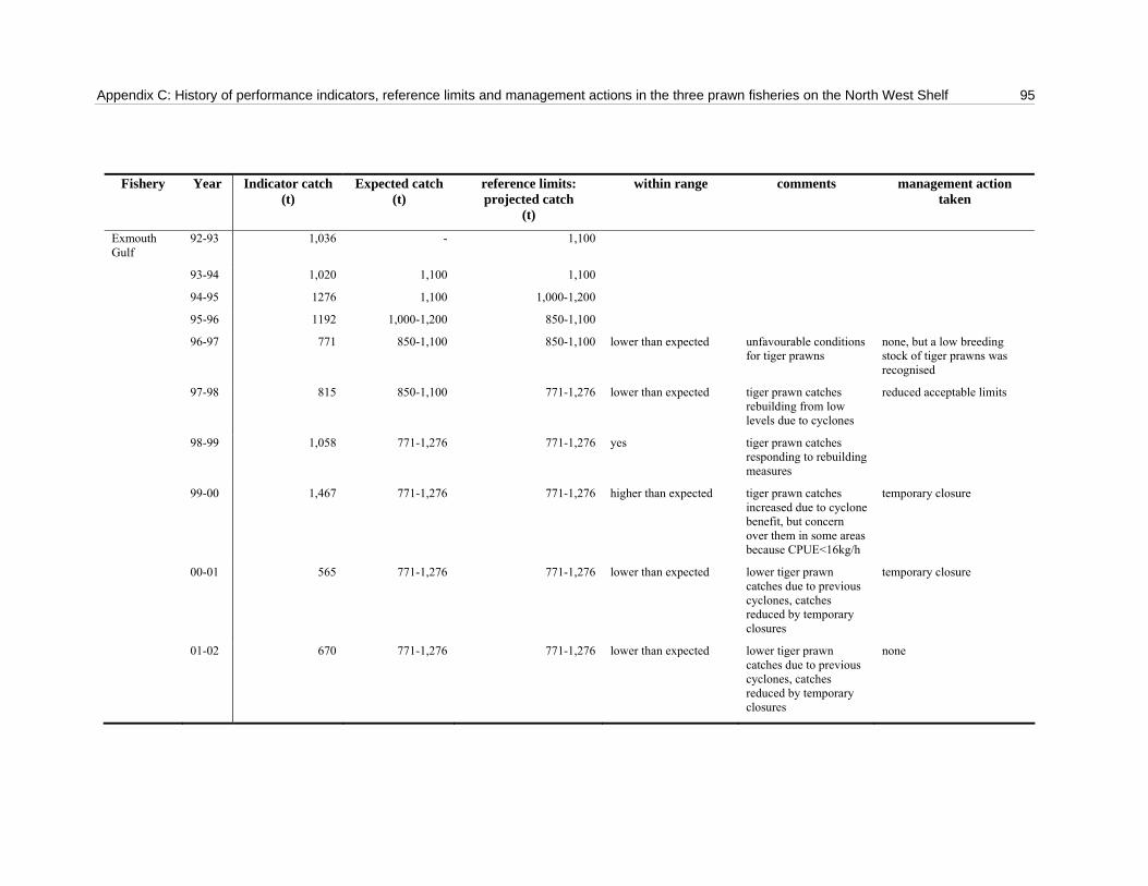
Appendix C: History of performance indicators, reference limits and management actions in the three prawn fisheries on the North West Shelf 95
Fishery Year Indicator catch (t)
Expected catch (t)
reference limits: projected catch
(t)
within range comments management action taken
Exmouth Gulf
92-93 1,036 - 1,100
93-94 1,020 1,100 1,100
94-95 1276 1,100 1,000-1,200
95-96 1192 1,000-1,200 850-1,100
96-97 771 850-1,100 850-1,100 lower than expected unfavourable conditions for tiger prawns
none, but a low breeding stock of tiger prawns was recognised
97-98 815 850-1,100 771-1,276 lower than expected tiger prawn catches rebuilding from low levels due to cyclones
reduced acceptable limits
98-99 1,058 771-1,276 771-1,276 yes tiger prawn catches responding to rebuilding measures
99-00 1,467 771-1,276 771-1,276 higher than expected tiger prawn catches increased due to cyclone benefit, but concern over them in some areas because CPUE<16kg/h
temporary closure
00-01 565 771-1,276 771-1,276 lower than expected lower tiger prawn catches due to previous cyclones, catches reduced by temporary closures
temporary closure
01-02 670 771-1,276 771-1,276 lower than expected lower tiger prawn catches due to previous cyclones, catches reduced by temporary closures
none
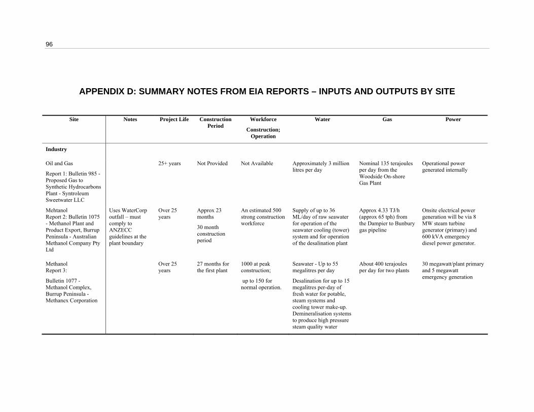
96
APPENDIX D: SUMMARY NOTES FROM EIA REPORTS – INPUTS AND OUTPUTS BY SITE
Site Notes Project Life Construction Period
Workforce
Construction; Operation
Water Gas Power
Industry
Oil and Gas
Report 1: Bulletin 985 - Proposed Gas to Synthetic Hydrocarbons Plant - Syntroleum Sweetwater LLC
25+ years Not Provided Not Available Approximately 3 million litres per day
Nominal 135 terajoules per day from the Woodside On-shore Gas Plant
Operational power generated internally
Mehtanol Report 2: Bulletin 1075 - Methanol Plant and Product Export, Burrup Peninsula - Australian Methanol Company Pty Ltd
Uses WaterCorp outfall – must comply to ANZECC guidelines at the plant boundary
Over 25 years
Approx 23 months
30 month construction period
An estimated 500 strong construction workforce
Supply of up to 36 ML/day of raw seawater for operation of the seawater cooling (tower) system and for operation of the desalination plant
Approx 4.33 TJ/h (approx 65 tph) from the Dampier to Bunbury gas pipeline
Onsite electrical power generation will be via 8 MW steam turbine generator (primary) and 600 kVA emergency diesel power generator.
Methanol Report 3:
Bulletin 1077 - Methanol Complex, Burrup Peninsula - Methanex Corporation
Over 25 years
27 months for the first plant
1000 at peak construction;
up to 150 for normal operation.
Seawater - Up to 55 megalitres per day
Desalination for up to 15 megalitres per-day of fresh water for potable, steam systems and cooling tower make-up. Demineralisation systems to produce high pressure steam quality water
About 400 terajoules per day for two plants
30 megawatt/plant primary and 5 megawatt emergency generation
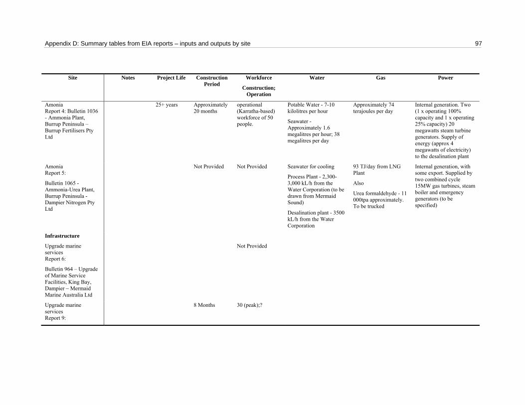
Appendix D: Summary tables from EIA reports – inputs and outputs by site 97
Site Notes Project Life Construction Period
Workforce
Construction; Operation
Water Gas Power
Amonia Report 4: Bulletin 1036 - Ammonia Plant, Burrup Peninsula – Burrup Fertilisers Pty Ltd
25+ years Approximately 20 months
operational (Karratha-based) workforce of 50 people.
Potable Water - 7-10 kilolitres per hour
Seawater - Approximately 1.6 megalitres per hour; 38 megalitres per day
Approximately 74 terajoules per day
Internal generation. Two (1 x operating 100% capacity and 1 x operating 25% capacity) 20 megawatts steam turbine generators. Supply of energy (approx 4 megawatts of electricity) to the desalination plant
Amonia Report 5:
Bulletin 1065 - Ammonia-Urea Plant, Burrup Peninsula - Dampier Nitrogen Pty Ltd
Not Provided Not Provided Seawater for cooling
Process Plant - 2,300-3,000 kL/h from the Water Corporation (to be drawn from Mermaid Sound)
Desalination plant - 3500 kL/h from the Water Corporation
93 TJ/day from LNG Plant
Also
Urea formaldehyde - 11 000tpa approximately. To be trucked
Internal generation, with some export. Supplied by two combined cycle 15MW gas turbines, steam boiler and emergency generators (to be specified)
Infrastructure
Upgrade marine services Report 6:
Bulletin 964 – Upgrade of Marine Service Facilities, King Bay, Dampier – Mermaid Marine Australia Ltd
Not Provided
Upgrade marine services Report 9:
8 Months 30 (peak);?
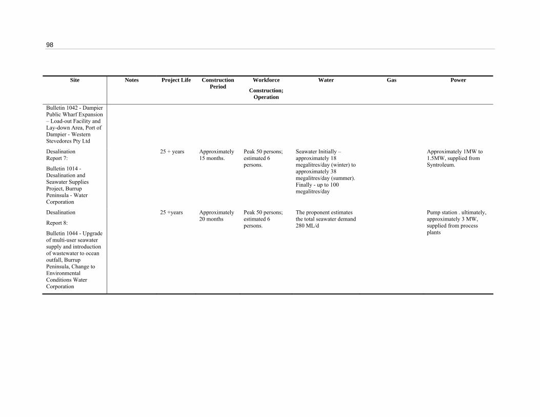
98
Site Notes Project Life Construction Period
Workforce
Construction; Operation
Water Gas Power
Bulletin 1042 - Dampier Public Wharf Expansion – Load-out Facility and Lay-down Area, Port of Dampier - Western Stevedores Pty Ltd
Desalination Report 7:
Bulletin 1014 - Desalination and Seawater Supplies Project, Burrup Peninsula - Water Corporation
25 + years Approximately 15 months.
Peak 50 persons; estimated 6 persons.
Seawater Initially – approximately 18 megalitres/day (winter) to approximately 38 megalitres/day (summer). Finally - up to 100 megalitres/day
Approximately 1MW to 1.5MW, supplied from Syntroleum.
Desalination
Report 8:
Bulletin 1044 - Upgrade of multi-user seawater supply and introduction of wastewater to ocean outfall, Burrup Peninsula, Change to Environmental Conditions Water Corporation
25 +years Approximately 20 months
Peak 50 persons; estimated 6 persons.
The proponent estimates the total seawater demand 280 ML/d
Pump station . ultimately, approximately 3 MW, supplied from process plants
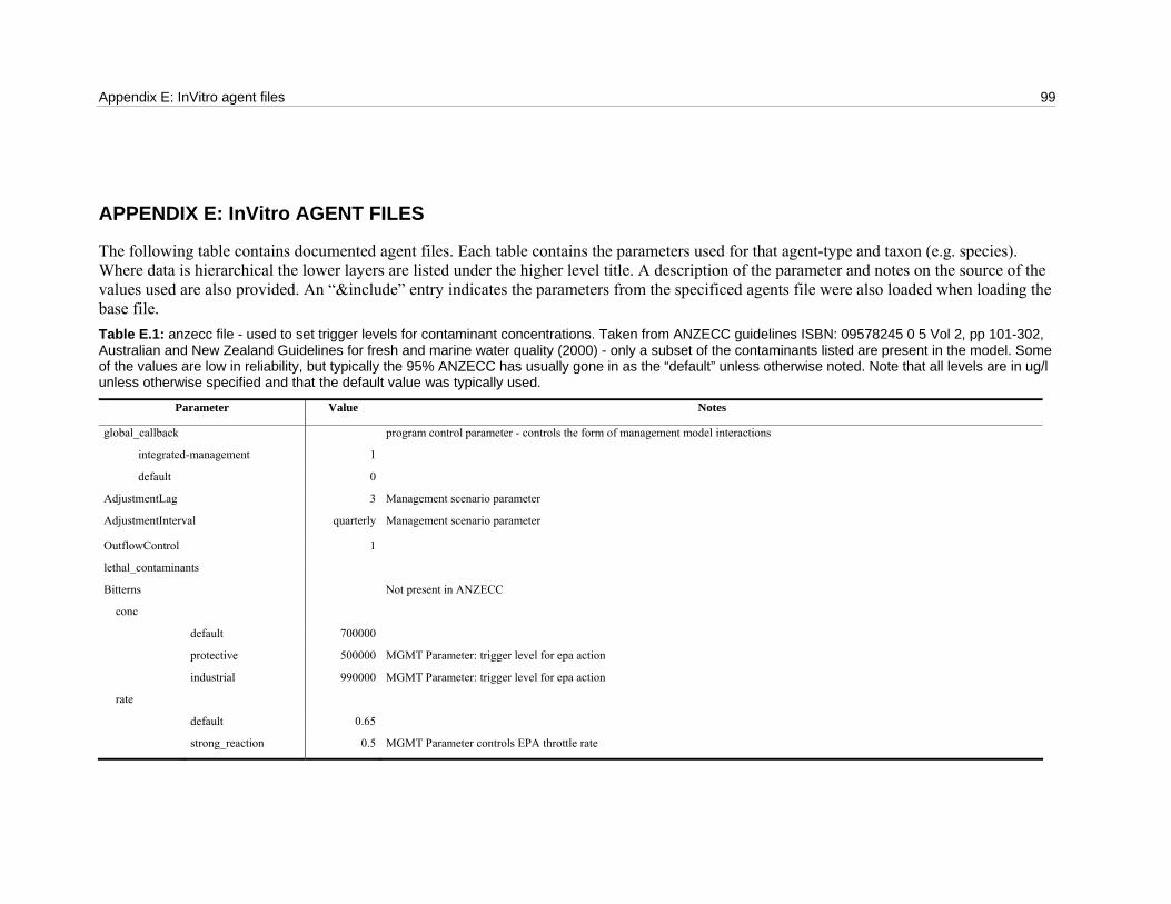
Appendix E: InVitro agent files 99
APPENDIX E: InVitro AGENT FILES
The following table contains documented agent files. Each table contains the parameters used for that agent-type and taxon (e.g. species). Where data is hierarchical the lower layers are listed under the higher level title. A description of the parameter and notes on the source of the values used are also provided. An “&include” entry indicates the parameters from the specificed agents file were also loaded when loading the base file. Table E.1: anzecc file - used to set trigger levels for contaminant concentrations. Taken from ANZECC guidelines ISBN: 09578245 0 5 Vol 2, pp 101-302, Australian and New Zealand Guidelines for fresh and marine water quality (2000) - only a subset of the contaminants listed are present in the model. Some of the values are low in reliability, but typically the 95% ANZECC has usually gone in as the “default” unless otherwise noted. Note that all levels are in ug/l unless otherwise specified and that the default value was typically used.
Parameter Value Notes
global_callback program control parameter - controls the form of management model interactions
integrated-management 1
default 0
AdjustmentLag 3 Management scenario parameter
AdjustmentInterval quarterly Management scenario parameter
OutflowControl 1
lethal_contaminants
Bitterns Not present in ANZECC
conc
default 700000
protective 500000 MGMT Parameter: trigger level for epa action
industrial 990000 MGMT Parameter: trigger level for epa action
rate
default 0.65
strong_reaction 0.5 MGMT Parameter controls EPA throttle rate
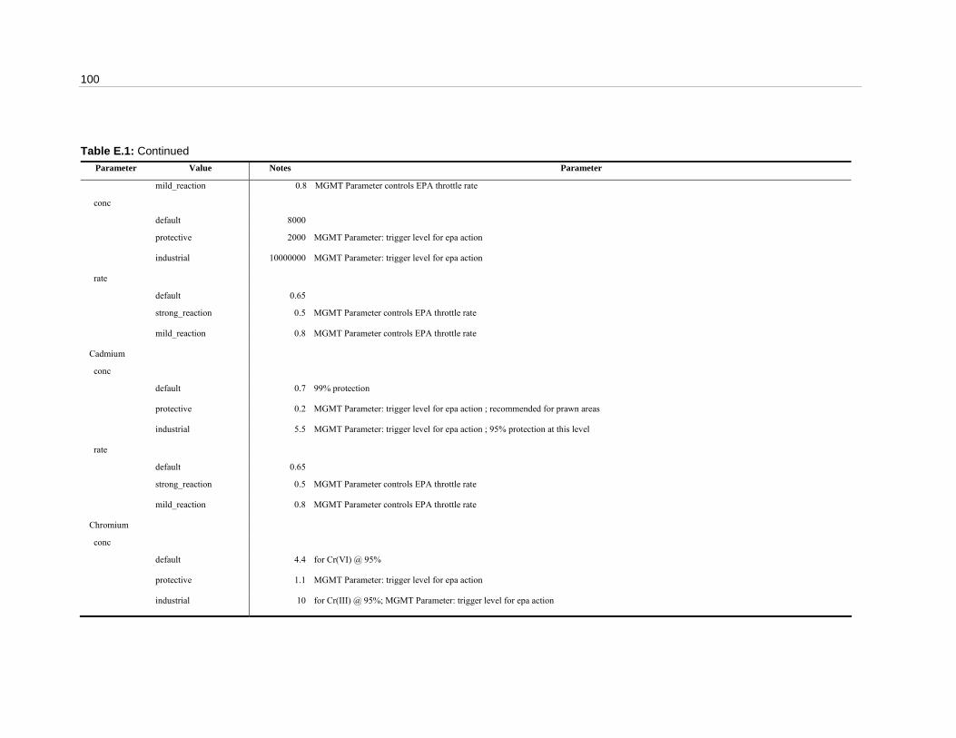
100
Table E.1: Continued Parameter Value Notes Parameter
mild_reaction 0.8 MGMT Parameter controls EPA throttle rate
conc
default 8000
protective 2000 MGMT Parameter: trigger level for epa action
industrial 10000000 MGMT Parameter: trigger level for epa action
rate
default 0.65
strong_reaction 0.5 MGMT Parameter controls EPA throttle rate
mild_reaction 0.8 MGMT Parameter controls EPA throttle rate
Cadmium
conc
default 0.7 99% protection
protective 0.2 MGMT Parameter: trigger level for epa action ; recommended for prawn areas
industrial 5.5 MGMT Parameter: trigger level for epa action ; 95% protection at this level
rate
default 0.65
strong_reaction 0.5 MGMT Parameter controls EPA throttle rate
mild_reaction 0.8 MGMT Parameter controls EPA throttle rate
Chromium
conc
default 4.4 for Cr(VI) @ 95%
protective 1.1 MGMT Parameter: trigger level for epa action
industrial 10 for Cr(III) @ 95%; MGMT Parameter: trigger level for epa action
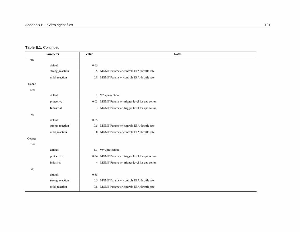
Appendix E: InVitro agent files 101
Table E.1: Continued
Parameter Value Notes
rate
default 0.65
strong_reaction 0.5 MGMT Parameter controls EPA throttle rate
mild_reaction 0.8 MGMT Parameter controls EPA throttle rate
Cobalt
conc
default 1 95% protection
protective 0.03 MGMT Parameter: trigger level for epa action
Industrial 3 MGMT Parameter: trigger level for epa action
rate
default 0.65
strong_reaction 0.5 MGMT Parameter controls EPA throttle rate
mild_reaction 0.8 MGMT Parameter controls EPA throttle rate
Copper
conc
default 1.3 95% protection
protective 0.04 MGMT Parameter: trigger level for epa action
industrial 4 MGMT Parameter: trigger level for epa action
rate
default 0.65
strong_reaction 0.5 MGMT Parameter controls EPA throttle rate
mild_reaction 0.8 MGMT Parameter controls EPA throttle rate

102
Table E.1: Continued
Parameter Value Notes
Lead
conc
default 4.4 for Cr(VI) @ 95%
protective 1.1 MGMT Parameter: trigger level for epa action
industrial 10 for Cr(III) @ 95%; MGMT Parameter: trigger level for epa action
rate
default 0.65
strong_reaction 0.5 MGMT Parameter controls EPA throttle rate
mild_reaction 0.8 MGMT Parameter controls EPA throttle rate
Manganese
conc 80 low reliability
rate
default 0.65
strong_reaction 0.5 MGMT Parameter controls EPA throttle rate
mild_reaction 0.8 MGMT Parameter controls EPA throttle rate
conc 3 low reliability
default 0.65
strong_reaction 0.5 MGMT Parameter controls EPA throttle rate
mild_reaction 0.8 MGMT Parameter controls EPA throttle rate
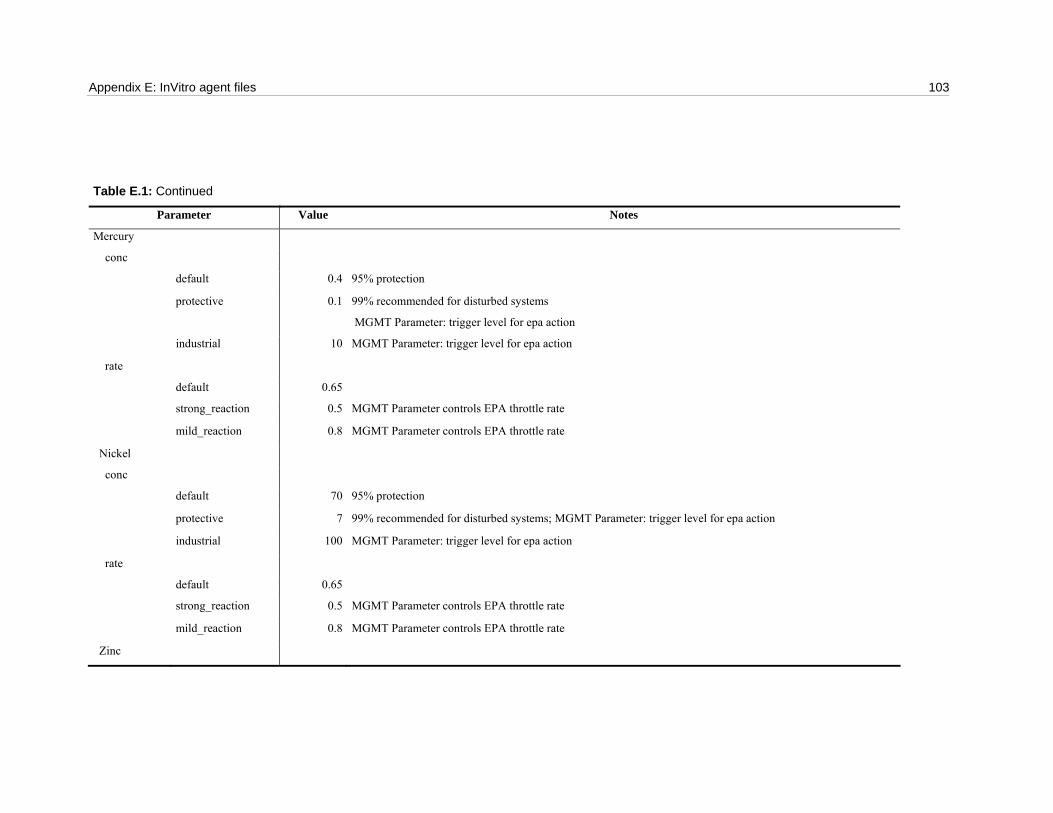
Appendix E: InVitro agent files 103
Table E.1: Continued
Parameter Value Notes
Mercury
conc
default 0.4 95% protection
protective 0.1 99% recommended for disturbed systems
MGMT Parameter: trigger level for epa action
industrial 10 MGMT Parameter: trigger level for epa action
rate
default 0.65
strong_reaction 0.5 MGMT Parameter controls EPA throttle rate
mild_reaction 0.8 MGMT Parameter controls EPA throttle rate
Nickel
conc
default 70 95% protection
protective 7 99% recommended for disturbed systems; MGMT Parameter: trigger level for epa action
industrial 100 MGMT Parameter: trigger level for epa action
rate
default 0.65
strong_reaction 0.5 MGMT Parameter controls EPA throttle rate
mild_reaction 0.8 MGMT Parameter controls EPA throttle rate
Zinc
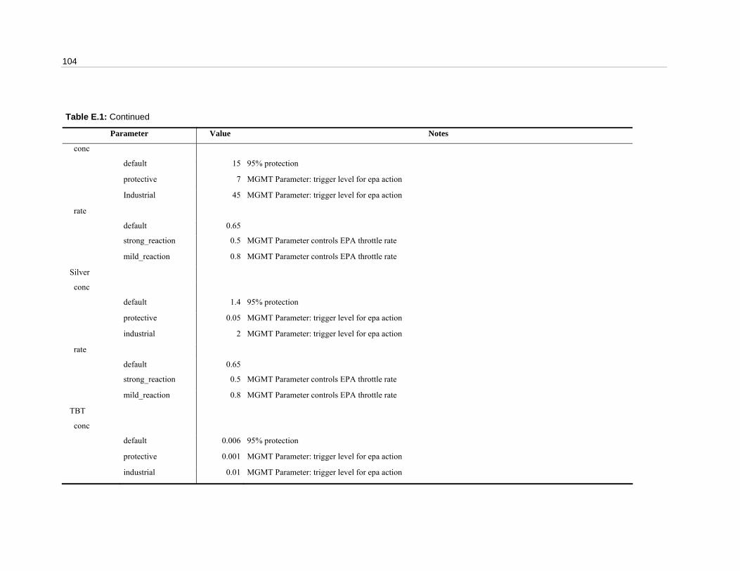
104
Table E.1: Continued
Parameter Value Notes
conc
default 15 95% protection
protective 7 MGMT Parameter: trigger level for epa action
Industrial 45 MGMT Parameter: trigger level for epa action
rate
default 0.65
strong_reaction 0.5 MGMT Parameter controls EPA throttle rate
mild_reaction 0.8 MGMT Parameter controls EPA throttle rate
Silver
conc
default 1.4 95% protection
protective 0.05 MGMT Parameter: trigger level for epa action
industrial 2 MGMT Parameter: trigger level for epa action
rate
default 0.65
strong_reaction 0.5 MGMT Parameter controls EPA throttle rate
mild_reaction 0.8 MGMT Parameter controls EPA throttle rate
TBT
conc
default 0.006 95% protection
protective 0.001 MGMT Parameter: trigger level for epa action
industrial 0.01 MGMT Parameter: trigger level for epa action

Appendix E: InVitro agent files 105
Table E.1: Continued
Parameter Value Notes
rate
default 0.65
strong_reaction 0.5 MGMT Parameter controls EPA throttle rate
mild_reaction 0.8 MGMT Parameter controls EPA throttle rate
Tin
conc
default 6 95% protection
protective 1 MGMT Parameter: trigger level for epa action
industrial 10 MGMT Parameter: trigger level for epa action
Tin
rate
Default 0.65
strong_reaction 0.5 MGMT Parameter controls EPA throttle rate
mild_reaction 0.8 MGMT Parameter controls EPA throttle rate
Oil
conc
Default 7000 low reliability
Protective 5000 MGMT Parameter: trigger level for epa action
Industrial 21000 MGMT Parameter: trigger level for epa action
rate
Default 0.65
strong_reaction 0.5 MGMT Parameter controls EPA throttle rate

106
Table E.1: Continued
Parameter Value Notes
mild_reaction 0.8 MGMT Parameter controls EPA throttle rate
Condensate
conc
Default 500 low reliability
Protective 200 MGMT Parameter: trigger level for epa action
Industrial 1500 MGMT Parameter: trigger level for epa action
rate
Default 0.65
strong_reaction 0.5 MGMT Parameter controls EPA throttle rate
mild_reaction 0.8 MGMT Parameter controls EPA throttle rate

Appendix E: InVitro agent files 107
Table E.2: contamination-prawns file (LC levels, uptake and decay rates). The values in this file were taken from the ASEAN documents unless otherwise specified. Not all the data in this file is used. Not all contaminants in the file are present in the simulation. The best values reported in the source documents were used.
Parameter Value Notes
logs_contamination program control parameter - sets whether this species writes contamination date to disk
default 1
NoContaminants 0
Intensive_tracking 1
contamination_track_interval daily program control parameter - determines how frequently tissueloads are written to file
tracks_contamination controls whether or not species interacts with contaminants
NoContaminants 0
default 0
fish 1
population 0
larva 0
blastula 0
contaminants
AccumToxin
conc 0
LDT 3.46E+08 duration of LC trial from ASEAN document
LD50 4.60E+20 LC50 in ug/L*10e8 from ASEAN document
LD100 1.00E+21 LC100 in ug/L*10e8 (An upper bound - not necessarily the least upper bound)
Nbins 50
L_Uptake Linear and NonLinear uptake rates, calibrated to provide observable effect over time
default 0.003587 /day

108
Table E.2: Continued
Parameter Value Notes
low_uptake 0.003 /day
AccumToxin
L_Uptake
mid_uptake 0.003587 /day
high_uptake 0.004 /day
NL_Uptake
Linear and NonLinear uptake rates, calibrated to provide observable effect over time
default 1.00E-08
low_uptake 1.00E-09
high_uptake 1.00E-07
Halflife 10*year halflife of contaminant in the absence of additional input only relevant to prawns (estimated from Hashmi et al. 2000)
Bitterns
LDT Day duration of LC trial from ASEAN document
LD50 4.00E+07 LC50 in ug/L*10e8 from ASEAN document
LD100 1.20E+08 LC100 in ug/L*10e8 (An upper bound - not necessarily the least upper bound)
conc 0
L_Uptake 0 Linear and NonLinear uptake rates, calibrated to provide observable effect over time
NL_Uptake Linear and NonLinear uptake rates, calibrated to provide observable effect over time
default 0.000464
low_uptake 0.000164
high_uptake 0.000464
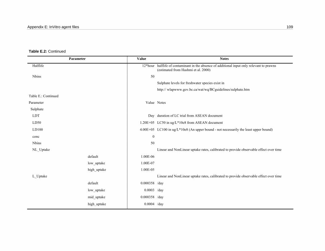
Appendix E: InVitro agent files 109
Table E.2: Continued
Parameter Value Notes
Halflife 12*hour halflife of contaminant in the absence of additional input only relevant to prawns (estimated from Hashmi et al. 2000)
Nbins 50
Sulphate levels for freshwater species exist in
http:// wlapwww.gov.bc.ca/wat/wq/BCguidelines/sulphate.htm
Table E.: Continued
Parameter Value Notes
Sulphate
LDT Day duration of LC trial from ASEAN document
LD50 1.20E+05 LC50 in ug/L*10e8 from ASEAN document
LD100 4.00E+05 LC100 in ug/L*10e8 (An upper bound - not necessarily the least upper bound)
conc 0
Nbins 50
NL_Uptake Linear and NonLinear uptake rates, calibrated to provide observable effect over time
default 1.00E-06
low_uptake 1.00E-07
high_uptake 1.00E-05
L_Uptake Linear and NonLinear uptake rates, calibrated to provide observable effect over time
default 0.000358 /day
low_uptake 0.0003 /day
mid_uptake 0.000358 /day
high_uptake 0.0004 /day
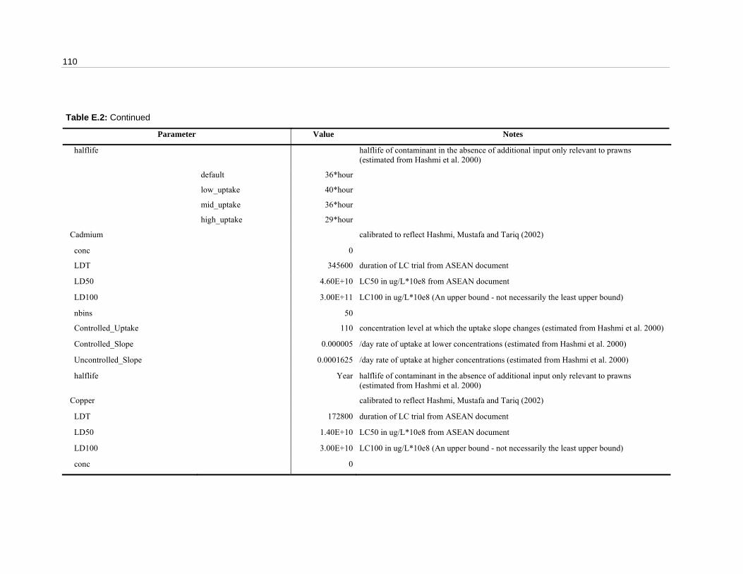
110
Table E.2: Continued
Parameter Value Notes
halflife halflife of contaminant in the absence of additional input only relevant to prawns (estimated from Hashmi et al. 2000)
default 36*hour
low_uptake 40*hour
mid_uptake 36*hour
high_uptake 29*hour
Cadmium calibrated to reflect Hashmi, Mustafa and Tariq (2002)
conc 0
LDT 345600 duration of LC trial from ASEAN document
LD50 4.60E+10 LC50 in ug/L*10e8 from ASEAN document
LD100 3.00E+11 LC100 in ug/L*10e8 (An upper bound - not necessarily the least upper bound)
nbins 50
Controlled_Uptake 110 concentration level at which the uptake slope changes (estimated from Hashmi et al. 2000)
Controlled_Slope 0.000005 /day rate of uptake at lower concentrations (estimated from Hashmi et al. 2000)
Uncontrolled_Slope 0.0001625 /day rate of uptake at higher concentrations (estimated from Hashmi et al. 2000)
halflife Year halflife of contaminant in the absence of additional input only relevant to prawns (estimated from Hashmi et al. 2000)
Copper calibrated to reflect Hashmi, Mustafa and Tariq (2002)
LDT 172800 duration of LC trial from ASEAN document
LD50 1.40E+10 LC50 in ug/L*10e8 from ASEAN document
LD100 3.00E+10 LC100 in ug/L*10e8 (An upper bound - not necessarily the least upper bound)
conc 0

Appendix E: InVitro agent files 111
Table E.2: Continued
Parameter Value Notes
NL_Uptake 0.00047 /day Linear and NonLinear uptake rates, calibrated to provide observable effect over time
L_Uptake 0.00035 /day Linear and NonLinear uptake rates, calibrated to provide observable effect over time
lambda 4.38E-08 decay rate of contaminant in the absence of additional input (unused)
Lead calibrated to reflect Hashmi, Mustafa and Tariq (2002)
LDT 345600 duration of LC trial from ASEAN document
LD50 2.85E+10 LC50 in ug/L*10e8 from ASEAN document
LD100 6.00E+10 LC100 in ug/L*10e8 (An upper bound - not necessarily the least upper bound)
conc 0
Controlled_Uptake 80 concentration level at which the uptake slope changes (estimated from Hashmi et al. 2000)
Controlled_Slope 0.000005 /day rate of uptake at lower concentrations (estimated from Hashmi et al. 2000)
Uncontrolled_Slope 0.0001825 /day rate of uptake at higher concentrations (estimated from Hashmi et al. 2000)
halflife 1.5*year halflife of contaminant in the absence of additional input only relevant to prawns (estimated from Hashmi et al. 2000)
Zinc
LDT 345600 duration of LC trial from ASEAN document
LD50 1850 LC50 in ug/L*10e8 from ASEAN document
LD100 4000 LC100 in ug/L*10e8 (An upper bound - not necessarily the least upper bound)
conc 0
Zinc
NL_Uptake
0.3 Linear and NonLinear uptake rates, calibrated to provide observable effect over time
L_Uptake 1.00E-05 Linear and NonLinear uptake rates, calibrated to provide observable effect over time

112
Table E.2: Continued
Parameter Value Notes
lambda 4.38E-08 decay rate of contaminant in the absence of additional input (unused)
Oil
LDT day duration of LC trial from ASEAN document
LD50 10 LC50 in ug/L*10e8 from ASEAN document
LD100 100 LC100 in ug/L*10e8 (An upper bound - not necessarily the least upper bound)
conc 0
NL_Uptake 0.1 Linear and NonLinear uptake rates, calibrated to provide observable effect over time
L_Uptake 1.00E-05 Linear and NonLinear uptake rates, calibrated to provide observable effect over time
lambda 1.00E-06 decay rate of contaminant in the absence of additional input (unused)
PFW
LDT day duration of LC trial from ASEAN document
LD50 100 LC50 in ug/L*10e8 from ASEAN document
LD100 1000 LC100 in ug/L*10e8 (An upper bound - not necessarily the least upper bound)
conc 0
NL_Uptake 0.1 Linear and NonLinear uptake rates, calibrated to provide observable effect over time
L_Uptake 1.00E-05 Linear and NonLinear uptake rates, calibrated to provide observable effect over time
Lambda 1.00E-06 decay rate of contaminant in the absence of additional input (unused)

Appendix E: InVitro agent files 113
Table E.3: contamination-oysters file (LC levels, uptake and decay rates). The values in this file were taken from the ASEAN documents unless otherwise specified. Not all the data in this file is used. Not all contaminants in the file are present in the simulation. The best values reported in the source documents were used.
Parameter Value Notes
logs_contamination program control parameter - sets whether this species writes contamination date to disk
NoContaminants 0
default 1
contamination_track_interval daily program control parameter - determines how frequently tissueloads are written to file
tracks_contamination controls whether or not species interacts with contaminants
NoContaminants 0
default 0
fish 1
population 0
larva 0
blastula 0
contaminants
AccumToxin
conc 0
LDT 3.46E+08 duration of LC trial from ASEAN document
LD50 4.60E+20 LC50 in ug/L*10e8 from ASEAN document
LD100 1.00E+21 LC100 in ug/L*10e8 (An upper bound - not necessarily the least upper bound)
nbins 50
L_Uptake Linear and NonLinear uptake rates, calibrated to provide observable effect over time
default 0.003587162 /day
low_uptake 0.003 /day
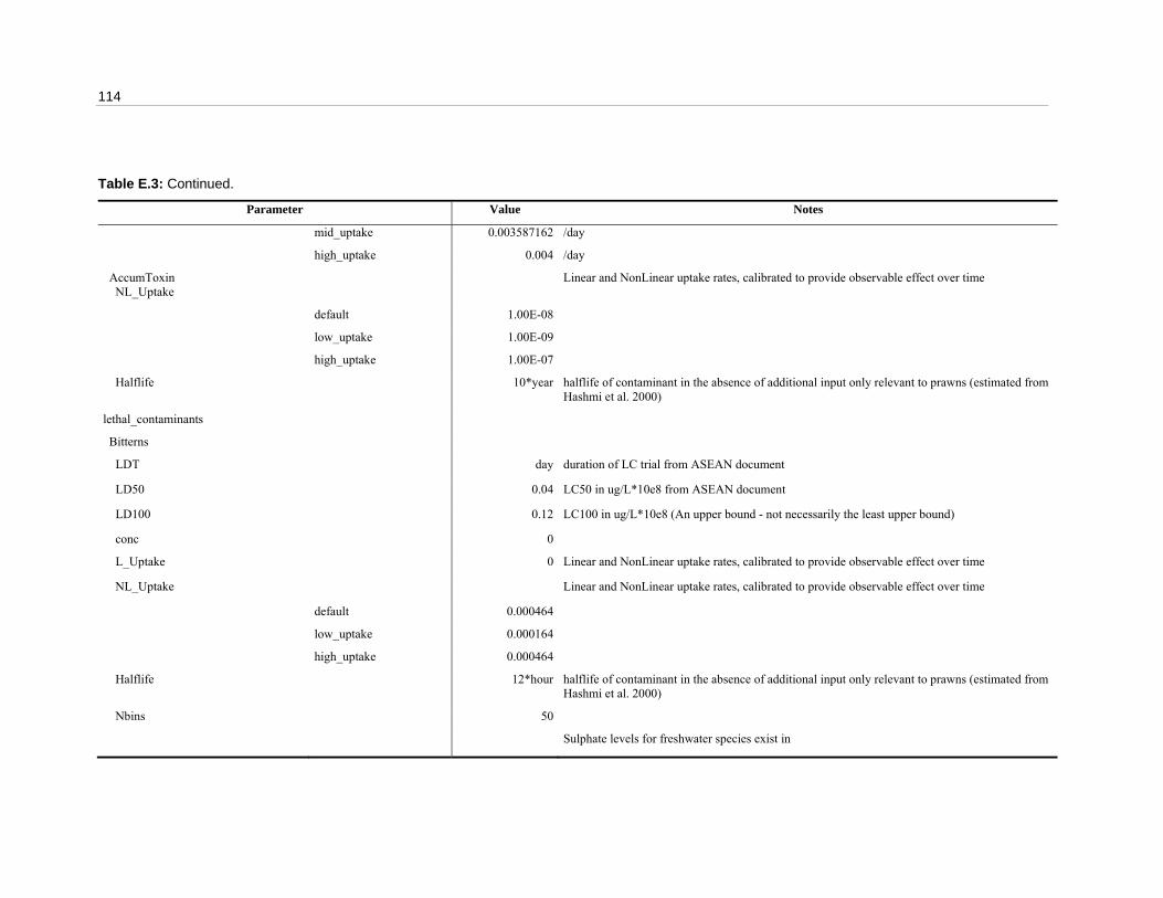
114
Table E.3: Continued.
Parameter Value Notes
mid_uptake 0.003587162 /day
high_uptake 0.004 /day
AccumToxin NL_Uptake
Linear and NonLinear uptake rates, calibrated to provide observable effect over time
default 1.00E-08
low_uptake 1.00E-09
high_uptake 1.00E-07
Halflife 10*year halflife of contaminant in the absence of additional input only relevant to prawns (estimated from Hashmi et al. 2000)
lethal_contaminants
Bitterns
LDT day duration of LC trial from ASEAN document
LD50 0.04 LC50 in ug/L*10e8 from ASEAN document
LD100 0.12 LC100 in ug/L*10e8 (An upper bound - not necessarily the least upper bound)
conc 0
L_Uptake 0 Linear and NonLinear uptake rates, calibrated to provide observable effect over time
NL_Uptake Linear and NonLinear uptake rates, calibrated to provide observable effect over time
default 0.000464
low_uptake 0.000164
high_uptake 0.000464
Halflife 12*hour halflife of contaminant in the absence of additional input only relevant to prawns (estimated from Hashmi et al. 2000)
Nbins 50
Sulphate levels for freshwater species exist in

Appendix E: InVitro agent files 115
Parameter Value Notes
http://wlapwww.gov.bc.ca/wat/wq/BCguidelines/sulphate.html
Sulphate
LDT day duration of LC trial from ASEAN document
LD50 5900 LC50 in ug/L*10e8 from ASEAN document
LD100 20000 LC100 in ug/L*10e8 (An upper bound - not necessarily the least upper bound)
conc 0
Nbins 50
NL_Uptake Linear and NonLinear uptake rates, calibrated to provide observable effect over time
default 1.00E-06
low_uptake 1.00E-07
high_uptake 1.00E-05
L_Uptake Linear and NonLinear uptake rates, calibrated to provide observable effect over time
default 0.0003587162 /day
low_uptake 0.0003 /day
mid_uptake 0.0003587162 /day
high_uptake 0.0004 /day
halflife halflife of contaminant in the absence of additional input only relevant to prawns (estimated from Hashmi et al. 2000)
default 36*hour
low_uptake 40*hour
mid_uptake 36*hour
high_uptake 29*hour
Cadmium
conc 0

116
Table E.3: Continued.
Parameter Value Notes
LDT 345600 duration of LC trial from ASEAN document
LD50 2210 LC50 in ug/L*10e8 from ASEAN document
LD100 1000 LC100 in ug/L*10e8 (An upper bound - not necessarily the least upper bound)
nbins 50
L_Uptake Linear and NonLinear uptake rates, calibrated to provide observable effect over time
default 0.003587162 /day
low_uptake 0.003 /day
mid_uptake 0.003587162 /day
high_uptake 0.004 /day
NL_Uptake Linear and NonLinear uptake rates, calibrated to provide observable effect over time
default 1.00E-08
low_uptake 1.00E-09
high_uptake 1.00E-07
halflife 10*year halflife of contaminant in the absence of additional input only relevant to prawns (estimated from Hashmi et al. 2000)
Copper
LDT 172800 duration of LC trial from ASEAN document
LD50 2440 LC50 in ug/L*10e8 from ASEAN document
LD100 4840 LC100 in ug/L*10e8 (An upper bound - not necessarily the least upper bound)
conc 0
NL_Uptake 0.3 Linear and NonLinear uptake rates, calibrated to provide observable effect over time
L_Uptake 1.00E-05 Linear and NonLinear uptake rates, calibrated to provide observable effect over time
lambda 4.38E-08 decay rate of contaminant in the absence of additional input (unused)
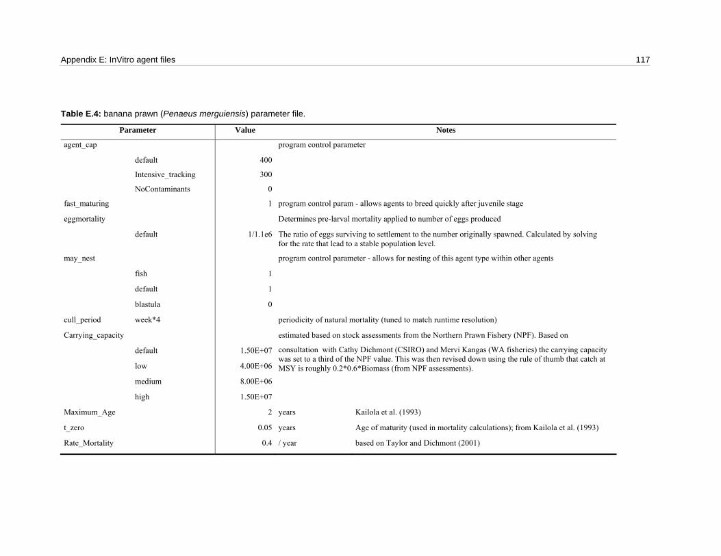
Appendix E: InVitro agent files 117
Table E.4: banana prawn (Penaeus merguiensis) parameter file.
Parameter Value Notes
agent_cap program control parameter
default 400
Intensive_tracking 300
NoContaminants 0
fast_maturing 1 program control param - allows agents to breed quickly after juvenile stage
eggmortality Determines pre-larval mortality applied to number of eggs produced
default 1/1.1e6 The ratio of eggs surviving to settlement to the number originally spawned. Calculated by solving for the rate that lead to a stable population level.
may_nest program control parameter - allows for nesting of this agent type within other agents
fish 1
default 1
blastula 0
cull_period week*4 periodicity of natural mortality (tuned to match runtime resolution)
Carrying_capacity
default 1.50E+07
low 4.00E+06
medium 8.00E+06
estimated based on stock assessments from the Northern Prawn Fishery (NPF). Based on
consultation with Cathy Dichmont (CSIRO) and Mervi Kangas (WA fisheries) the carrying capacity was set to a third of the NPF value. This was then revised down using the rule of thumb that catch at MSY is roughly 0.2*0.6*Biomass (from NPF assessments).
high 1.50E+07
Maximum_Age 2 years Kailola et al. (1993)
t_zero 0.05 years Age of maturity (used in mortality calculations); from Kailola et al. (1993)
Rate_Mortality 0.4 / year based on Taylor and Dichmont (2001)

118
Table E.4: Continued
Parameter Value Notes
Catastrophic_Mortality Mortality rate during catastrophic storm event
default 0.15 / event Guesstimate based on expert opinion and information in Taylor and Dichmont (2001) and Kailola et al. (1993)
low 0.3 / event Maximum value from guesstimate’s credible range
medium 0.15 / event Guesstimate based on expert opinion and information in Taylor and Dichmont (2001) and Kailola et al. (1993)
high 0.07 / event Minimum value from guesstimate’s credible range
Speed 0.08 metres / second Cruising speed; Hill (1985)
MaxSpeed 1.8 metres / second Hill (1985)
SearchRadiusExponent 2 governs how far afield we assume organisms can detect conditions (estimated based on velocity)
Directional_variability 0.2 degree to which they remain moving in a single facing (direction); calibrated
Speed_variability 0.07 stochastic variability in wandering speed; calculated by comparing crusing and maximum speeds in FISHBASE (2005)
Traverse_Time 1 months Time taken to cross the entire NWS if swimming directly; calculated from swimming speed, weighted by degree of aggregation (of agent – so populations took longer than fish)
Length_t 0.15 Coefficient in length-weight relationship (using length = pow(mass,ln(Length_t)/ln(Mass_t)))
Mass_t 0.03 Coefficient in length-weight relationship (using length = pow(mass,ln(Length_t)/ln(Mass_t)))
IndividualMass 0.03 Typical mass (kg) of an individual; direct measurement
Width_a 0.015 dimensions of organism; directly measured
Gape/Width 0.005 ratio of gape to width (estimated from direct measurements)
Capacity 0.3 gut capacity as a proportion of length (estimate from direct measurements)

Appendix E: InVitro agent files 119
Table E.4: Continued
Parameter Value Notes
Metabolism 0 kg of food burned per second determines if organisms must hunt or we assume adequate food (later assumed for MSE runs here)
Max_mass Upper limit of mass
default 0.07 kg Kailola et al. (1993)
mass_lambda 0.6 specified in years; for age-mass equation (tuned to give realistic age spans given known masses)
Safe_Range 6 six times the cruising speed estimated from visibility ranges; not used when adequate food assumed
Neighbourhood 0
Perception_Range 20 times the cruising speed The range at which prey may be detected; estimated from visibility ranges; not used when adequate food assumed
Eating_Range 1 seconds How close it must get seconds to it's prey (assuming the prey isn't “safe”) – the temporal range at which prey may be detected (a time not a distance measure as have known lunge speed for attack – see Gray et al. (2006) for formulation)
spatialLarvalFactor 1E-11 calibrated to give a plausible stock-recruit relationship
Fecundity_rate 1200000 mass based correction to maximum fecundity (calibrated to match field spawning rates – as opposed to laboratory determined maximum egg production)
Fecundity eggs / female at maximum size Maximum potential fecundity rate; Kailola et al. (1993)
default 7200000
low 5500000
medium 7200000
high 8500000
testing 2000
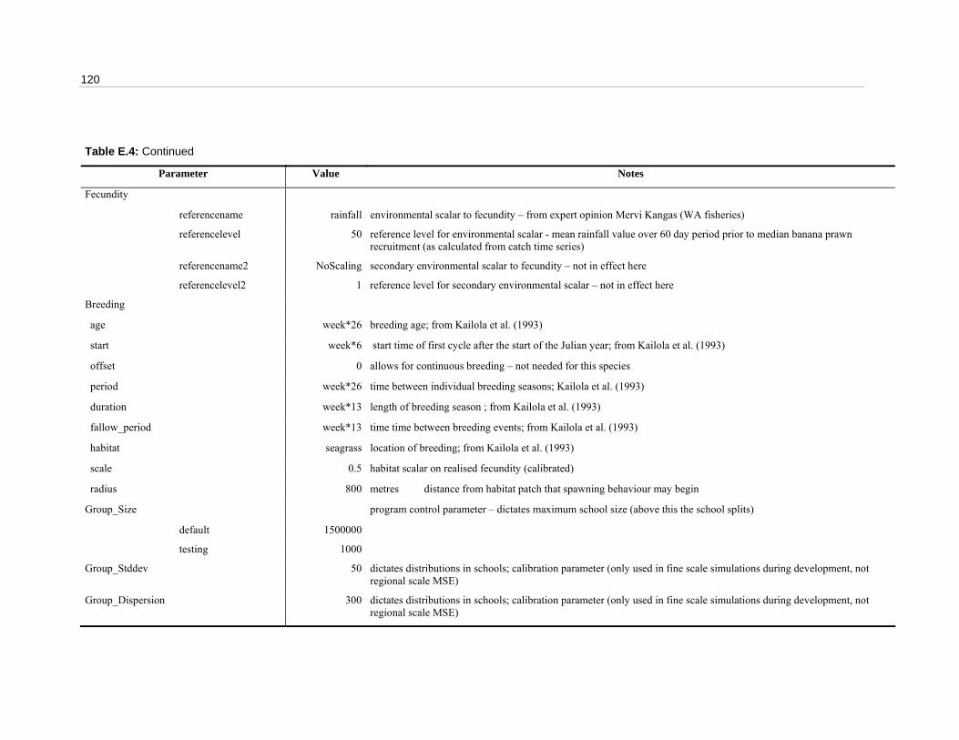
120
Table E.4: Continued
Parameter Value Notes
Fecundity
referencename rainfall environmental scalar to fecundity – from expert opinion Mervi Kangas (WA fisheries)
referencelevel 50 reference level for environmental scalar - mean rainfall value over 60 day period prior to median banana prawn recruitment (as calculated from catch time series)
referencename2 NoScaling secondary environmental scalar to fecundity – not in effect here
referencelevel2 1 reference level for secondary environmental scalar – not in effect here
Breeding
age week*26 breeding age; from Kailola et al. (1993)
start week*6 start time of first cycle after the start of the Julian year; from Kailola et al. (1993)
offset 0 allows for continuous breeding – not needed for this species
period week*26 time between individual breeding seasons; Kailola et al. (1993)
duration week*13 length of breeding season ; from Kailola et al. (1993)
fallow_period week*13 time time between breeding events; from Kailola et al. (1993)
habitat seagrass location of breeding; from Kailola et al. (1993)
scale 0.5 habitat scalar on realised fecundity (calibrated)
radius 800 metres distance from habitat patch that spawning behaviour may begin
Group_Size program control parameter – dictates maximum school size (above this the school splits)
default 1500000
testing 1000
Group_Stddev 50 dictates distributions in schools; calibration parameter (only used in fine scale simulations during development, not regional scale MSE)
Group_Dispersion 300 dictates distributions in schools; calibration parameter (only used in fine scale simulations during development, not regional scale MSE)

Appendix E: InVitro agent files 121
Table E.4: Continued
Parameter Value Notes
Group_Terminal when schools drop below this they are culled (if they can not merge first)
default 2000 group size below which school disperses
testing 20
Group_Must_Merge program control parameter dictating at what points schools try to merge with other schools of same taxon
default 20000 group must try and merge if it gets this low
testing 10
merge_radius_scale 200 merge radius (to merge must be within this radius in m) – typically set to about 20000x speed
Bored_Tick Maximum standard time step length
default week
very_fast day
fast week
slow week*4
Tick_Length Typical time step length
default week
very_fast 3600 seconds
fast day
moderate week
slow 2*week
Excited_Tick Standard time step length if in active state
default 1.5*hour seconds
very_fast 60 seconds

122
Table E.4: Continued
Parameter Value Notes
fast 3600 seconds
slow 600 seconds
Minimum_Depth -0.5 metres minimum preferred depth; Kailola et al. (1993)
Best_Depth -20 metres median preferred depth; Kailola et al. (1993)
Maximum_Depth -40 metres maximum preferred depth; Kailola et al. (1993)
Minimum_Sea_Depth -1 metres minimum depth typically used in marine waters (used to constrain locations in scenarios)
Maximum_Sea_Depth maximum depth typically reached in marine waters (often used to constrain the populations to specific locations for fine scale simulations)
default -50
very_shallow -18 used when retaining them within Nickol Bay (for contaminant trials)
shallow -20
large_range -70 metres
full_range -90 metres Kailola et al. (1993)
radius 10000 metres school extent
trawl_efficiency 0.1 efficiency of trawlers against species (analogous to selectivity in the population agents); set using expert opinion
spatialCatchFactor 0.05 calibrated to minimise differences between observed and predicted catches
selMass 0.05 kg mass juveniles when first susceptible to fishing (estimated)
assess_environment 1 flag to show whether species seeks favourable environments
Awareness_type 0 0 for fine scale awareness, 1 for large scale
program control parameter – dictating resolution of adviser agent interrogation (see Gray et al. 2005)

Appendix E: InVitro agent files 123
Table E.4: Continued
Parameter Value Notes
ScalingBestSeaDepth
default 0.0001 Weighting for influence of preferred depth in guiding habitat selection
Mass0 0.001 kg mass of individual fish larvae at notional hatching point
FastMaturation 1 1 = can reproduce soon after recruiting to adult population
Larva Juvenile parameters
MetabolismType 4 type of metabolism used: 1for cull if biomass is greater than carrying capacity, 2 for false metabolism, 3 for true animal metabolism and 4 for false metabolism and periodic density dependent cull (i.e. basically determines if organisms must hunt or we assume adequate food – the later assumed for MSE runs here)
tick_length 1200 seconds Typical time step length for juvenile age stages
bored_tick 81400 seconds Maximum standard time step length for juvenile age stages
alarmed_tick 600 seconds Standard time step length if in active state for juvenile age stages
head_for 1 flag setting whether they head for random spot or closest when recruiting or settling: (1 for heading for closest, 0 for heading for random)
trawl_efficiency 0 efficiency of trawlers against juveniles of this species (expert opinion, Neil Lonergan pers. comm.)
projection_efficiency_scalar 1 scalar on fishing efficiency so no discontinuity from historical to projection treatement (given different spatial scales of operation)
radius 10000 metres Radius of juvenile patch / school (estimated from aerial photographs)
spatialLarvalFactor 1E-11 settlement “stock-recruit” relationship scalar – calibrated to give plausible overall stock-recruit relationship
First Parameters for first age phase of larval agents
tracer_minor 3 flag to indicate form of advection used (3 means vertices are advected)
Current_K 0.4 metres / second coefficient for movement of unsettled larva with currents; calibrated so that observed time from spawning to settlement obtained and correct movement patterns seen
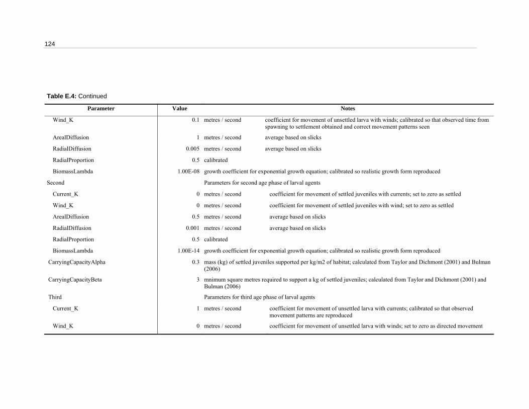
124
Table E.4: Continued
Parameter Value Notes
Wind_K 0.1 metres / second coefficient for movement of unsettled larva with winds; calibrated so that observed time from spawning to settlement obtained and correct movement patterns seen
ArealDiffusion 1 metres / second average based on slicks
RadialDiffusion 0.005 metres / second average based on slicks
RadialProportion 0.5 calibrated
BiomassLambda 1.00E-08 growth coefficient for exponential growth equation; calibrated so realistic growth form reproduced
Second Parameters for second age phase of larval agents
Current_K 0 metres / second coefficient for movement of settled juveniles with currents; set to zero as settled
Wind_K 0 metres / second coefficient for movement of settled juveniles with wind; set to zero as settled
ArealDiffusion 0.5 metres / second average based on slicks
RadialDiffusion 0.001 metres / second average based on slicks
RadialProportion 0.5 calibrated
BiomassLambda 1.00E-14 growth coefficient for exponential growth equation; calibrated so realistic growth form reproduced
CarryingCapacityAlpha 0.3 mass (kg) of settled juveniles supported per kg/m2 of habitat; calculated from Taylor and Dichmont (2001) and Bulman (2006)
CarryingCapacityBeta 3 mnimum square metres required to support a kg of settled juveniles; calculated from Taylor and Dichmont (2001) and Bulman (2006)
Third Parameters for third age phase of larval agents
Current_K 1 metres / second coefficient for movement of unsettled larva with currents; calibrated so that observed movement patterns are reproduced
Wind_K 0 metres / second coefficient for movement of unsettled larva with winds; set to zero as directed movement

Appendix E: InVitro agent files 125
Table E.4: Continued
Parameter Value Notes
Settling
age 1814400 seconds age when begin settling; Kailola et al. (1993)
radius 10000 metres distance from centre of bed of suitable habitat type that will settle
scale 0.5 scalar on habitat quality for settling
offset 1 offset on habitat quality for settling
habitat seagrass suitable settling habitat
habitat_type 4 habitat agent type (1 for data grid in file, 2 for habitat tracer agents, 3 for polyorganism agents, 4 for benthic agents, 5 for no agent type set and 6 for carrying capacity dependent settlement)
direction_travel 1 identifies whether swimming on-shore (1) or offshore (-1) or whereever (0) at this life stage
Recruitment
age 0.75 * year age when begin recruiting to adult population; Kailola et al. (1993)
radius 10000 distance from centre of bed of suitable habitat type that will recruit
temporal_radius time in blastula queue when “close enough” to recruit; calibrated to give realistic settlement patterns
default day * 13
short week
long 4 * week
scale 0.5 scalar on recruitment habitat preferences
offset 1 offset on recruitment habitat quality
habitat none identifies suitable recruiting habitat (none indicates no preference)
habitat_type 5 habitat agent type (1 for data grid in file, 2 for habitat tracer agents, 3 for polyorganism agents, 4 for benthic agents, 5 for no agent type set and 6 for carrying capacity dependent recruitment)
direction_travel 0 identifies whether swimming on-shore (1) or offshore (-1) or whereever (0) at this life stage

126
Table E.4: Continued
Parameter Value Notes
aggregate_rate 0.5 rate of polygon contraction when recruiting; calibrated to give smooth transition
Fears relative fear ranking (arbitary, with main predators given maximum ranking of about 0.9)
Fish 0.9
Tuna 0.9
Shark 0.9
habitat relative adult habitat ranking (arbitary, with most preferred habitat given maximum ranking of about 0.9)
Seagrass 0.9
Seabed 0.1
Seagrass_thresh 300000 total biomass (kg) in habitat grid cell; threshold biomass below which the animal is less interested in the habitat
&include Include/contamination-prawns

Appendix E: InVitro agent files 127
Table E.5: king prawn (Penaeus latisulcatus, Penaeus longistylus and Metapenaeus endeavouri, Metapenaeus ensis, Penaeus esculentus) parameter file.
Parameter Value Notes
agent_cap program control parameter
Default 400
NoContaminants 0
Intensive_tracking 300
fast_maturing 1 program control param - allows agents to breed quickly after juvenile stage
eggmortality Determines pre-larval mortality applied to number of eggs produced
Default 1/2e6 The ratio of eggs surviving to settlement to the number originally spawned. Calculated by solving for the rate that lead to a stable population level.
may_nest program control parameter - allows for nesting of this agent type within other agents
Fish 1
Default 1
Blastula 0
cull_period week*4 periodicity of natural mortality (tuned to runtime resolution)
Carrying_capacity
Default 1.67E+07
Low 8.00E+06
Medium 1.20E+07
High 1.60E+07
estimated based on stock assessments from the Northern Prawn Fishery (NPF). Based on consultation with Cathy Dichmont (CSIRO) and Mervi Kangas (WA fisheries) the carrying capacity was set to a third of the NPF value. This was then revised down using the rule of thumb that catch at MSY is roughly 0.2*0.6*Biomass (from NPF assessments).
Maximum_Age 4 years Kailola et al. (1993)
t_zero 0.05 years Age of maturity (used in mortality calculations); from Kailola et al. (1993)
Rate_Mortality 0.35 / year based on Taylor and Dichmont (2001)
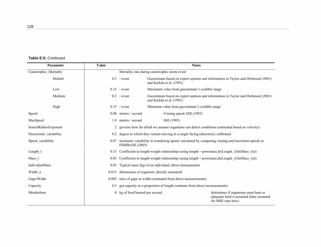
128
Table E.5: Continued
Parameter Value Notes
Catastrophic_Mortality Mortality rate during catastrophic storm event
Default 0.2 / event Guesstimate based on expert opinion and information in Taylor and Dichmont (2001) and Kailola et al. (1993)
Low 0.15 / event Maximum value from guesstimate’s credible range
Medium 0.2 / event Guesstimate based on expert opinion and information in Taylor and Dichmont (2001) and Kailola et al. (1993)
High 0.15 / event Minimum value from guesstimate’s credible range
Speed 0.08 metres / second Crusing speed; Hill (1985)
MaxSpeed 1.8 metres / second Hill (1985)
SearchRadiusExponent 2 governs how far afield we assume organisms can detect conditions (estimated based on velocity)
Directional_variability 0.2 degree to which they remain moving in a single facing (direction); calibrated
Speed_variability 0.07 stochastic variability in wandering speed; calculated by comparing crusing and maximum speeds in FISHBASE (2005)
Length_t 0.15 Coefficient in length-weight relationship (using length = pow(mass,ln(Length_t)/ln(Mass_t))))
Mass_t 0.03 Coefficient in length-weight relationship (using length = pow(mass,ln(Length_t)/ln(Mass_t))))
IndividualMass 0.03 Typical mass (kg) of an individual; direct measurement
Width_a 0.015 dimensions of organism; directly measured
Gape/Width 0.005 ratio of gape to width (estimated from direct measurements)
Capacity 0.3 gut capacity as a proportion of length (estimate from direct measurements)
Metabolism 0 kg of food burned per second determines if organisms must hunt or adequate food is assumed (later assumed for MSE runs here)

Appendix E: InVitro agent files 129
Table E.5: Continued
Parameter Value Notes
Max_mass Upper limit of mass
default 0.1 kg Kailola et al. (1993)
mass_lambda 0.6 specified in years; for age-mass equation (tuned to give realistic age spans given known masses)
Safe_Range 6 six times the cruising speed estimated from visibility ranges; not used when adequate food assumed
Neighbourhood 0
Perception_Range 20 times the cruising speed range at which prey may be detected
Eating_Range 1 seconds How close it must get seconds to its prey (assuming the prey isn't “safe”) – the temporal range at which prey may be detected (a time not a distance measure as have known lunge speed for attack – see Gray et al. (2006) for formulation)
spatialLarvalFactor calibrated to give a plausible stock-recruit relationship
default 1E-11
low 4.5E-06
medium 2.5E-06
high 5.5E-07
Fecundity_rate 1000000 mass based correction to maximum fecundity (calibrated to match field spawning rates – as opposed to laboratory determined maximum egg production)
Fecundity eggs / female at maximum size Maximum potential fecundity rate; Kailola et al. (1993)
default 7500000
low 6000000
medium 7500000
high 10000000
testing 2000

130
Table E.5: Continued
Parameter Value Notes
referencename NoScaling environmental scalar to fecundity – not in effect here
referencelevel 1 reference level for environmental scalar – not in effect here
referencename2 NoScaling secondary environmental scalar to fecundity – not in effect here
referencelevel2 1 reference level for secondary environmental scalar – not in effect here
Breeding
age week*26 breeding age; from Kailola et al. (1993)
start week*32 start time of first cycle after the start of the Julian year; from Kailola et al. (1993)
offset 0 allows for continuous breeding – not needed for this species
period week*52 time between individual breeding seasons; Kailola et al. (1993)
duration week*26
fallow_period week*26 time time between breeding events; from Kailola et al. (1993)
habitat seagrass
scale 0.5 habitat scalar on realised fecundity (calibrated)
radius 800 metres distance from habitat patch that spawning behaviour may begin
Group_Size program control parameter – dictates maximum school size (above this the school splits)
default 2000000
testing 1000
Group_Stddev 50 dictates distributions in schools; calibration parameter (only used in fine scale simulations during development, not regional scale MSE)
Group_Dispersion 300 dictates distributions in schools; calibration parameter (only used in fine scale simulations during development, not regional scale MSE)
Group_Terminal when schools drop below this they are culled (if they can not merge first)
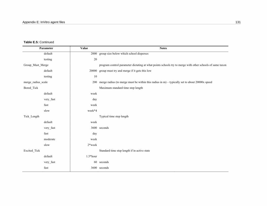
Appendix E: InVitro agent files 131
Table E.5: Continued
Parameter Value Notes
default 2000 group size below which school disperses
testing 20
Group_Must_Merge program control parameter dictating at what points schools try to merge with other schools of same taxon
default 20000 group must try and merge if it gets this low
testing 10
merge_radius_scale 200 merge radius (to merge must be within this radius in m) – typically set to about 20000x speed
Bored_Tick Maximum standard time step length
default week
very_fast day
fast week
slow week*4
Tick_Length Typical time step length
default week
very_fast 3600 seconds
fast day
moderate week
slow 2*week
Excited_Tick Standard time step length if in active state
default 1.5*hour
very_fast 60 seconds
fast 3600 seconds

132
Table E.5: Continued
Parameter Value Notes
slow 600 seconds
Minimum_Depth -0.1 metres minimum preferred depth; Kailola et al. (1993)
Best_Depth -10 metres median preferred depth; Kailola et al. (1993)
Maximum_Depth -40 metres maximum preferred depth; Kailola et al. (1993)
Minimum_Sea_Depth -0.1 metres minimum depth typically used in marine waters (used to constrain locations in scenarios)
Maximum_Sea_Depth maximum depth typically reached in marine waters (often used to constrain the populations to specific locations for fine scale simulations)
default -120
very_shallow -18 used when retaining them within Nickol Bay (for contaminant trials)
shallow -20
large_range -70 metres
full_range -90 metres Kailola et al. (1993)
radius 10000 metres school extent
trawl_efficiency 0.1 efficiency of trawlers against species (analogous to selectivity in the population agents); set using expert opinion
spatialCatchFactor 0.05 calibrated to minimise differences between observed and predicted catches
selMass 0.05 kg mass juveniles when first susceptible to fishing (estimated)
assess_environment 1 flag to show whether species seeks favourable environments
Awareness_type 0 0 for fine scale awareness, 1 for large scale program control parameter – dictating resolution of adviser agent interrogation (see Gray et al. (2006))
ScalingBestSeaDepth
default 0.0001 Weighting for influence of preferred depth in guiding habitat selection
Mass0 0.001 kg mass of individual fish larvae at notional hatching; must be greater than zero
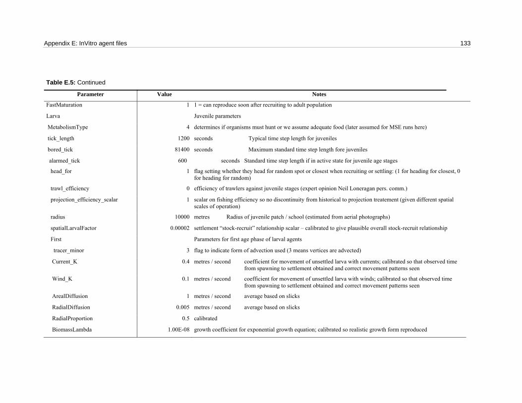
Appendix E: InVitro agent files 133
Table E.5: Continued
Parameter Value Notes
FastMaturation 1 1 = can reproduce soon after recruiting to adult population
Larva Juvenile parameters
MetabolismType 4 determines if organisms must hunt or we assume adequate food (later assumed for MSE runs here)
tick_length 1200 seconds Typical time step length for juveniles
bored_tick 81400 seconds Maximum standard time step length fore juveniles
alarmed_tick 600 seconds Standard time step length if in active state for juvenile age stages
head_for 1 flag setting whether they head for random spot or closest when recruiting or settling: (1 for heading for closest, 0 for heading for random)
trawl_efficiency 0 efficiency of trawlers against juvenile stages (expert opinion Neil Loneragan pers. comm.)
projection_efficiency_scalar 1 scalar on fishing efficiency so no discontinuity from historical to projection treatement (given different spatial scales of operation)
radius 10000 metres Radius of juvenile patch / school (estimated from aerial photographs)
spatialLarvalFactor 0.00002 settlement “stock-recruit” relationship scalar – calibrated to give plausible overall stock-recruit relationship
First Parameters for first age phase of larval agents
tracer_minor 3 flag to indicate form of advection used (3 means vertices are advected)
Current_K 0.4 metres / second coefficient for movement of unsettled larva with currents; calibrated so that observed time from spawning to settlement obtained and correct movement patterns seen
Wind_K 0.1 metres / second coefficient for movement of unsettled larva with winds; calibrated so that observed time from spawning to settlement obtained and correct movement patterns seen
ArealDiffusion 1 metres / second average based on slicks
RadialDiffusion 0.005 metres / second average based on slicks
RadialProportion 0.5 calibrated
BiomassLambda 1.00E-08 growth coefficient for exponential growth equation; calibrated so realistic growth form reproduced
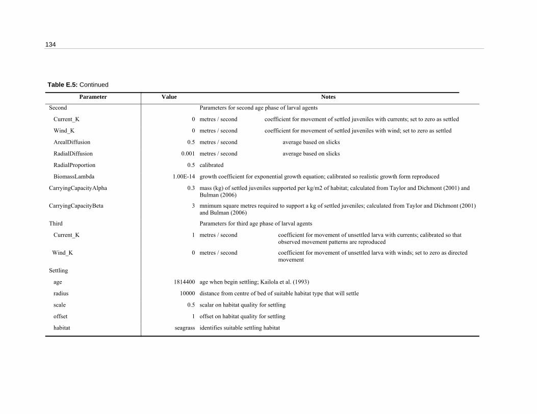
134
Table E.5: Continued
Parameter Value Notes
Second Parameters for second age phase of larval agents
Current_K 0 metres / second coefficient for movement of settled juveniles with currents; set to zero as settled
Wind_K 0 metres / second coefficient for movement of settled juveniles with wind; set to zero as settled
ArealDiffusion 0.5 metres / second average based on slicks
RadialDiffusion 0.001 metres / second average based on slicks
RadialProportion 0.5 calibrated
BiomassLambda 1.00E-14 growth coefficient for exponential growth equation; calibrated so realistic growth form reproduced
CarryingCapacityAlpha 0.3 mass (kg) of settled juveniles supported per kg/m2 of habitat; calculated from Taylor and Dichmont (2001) and Bulman (2006)
CarryingCapacityBeta 3 mnimum square metres required to support a kg of settled juveniles; calculated from Taylor and Dichmont (2001) and Bulman (2006)
Third Parameters for third age phase of larval agents
Current_K 1 metres / second coefficient for movement of unsettled larva with currents; calibrated so that observed movement patterns are reproduced
Wind_K 0 metres / second coefficient for movement of unsettled larva with winds; set to zero as directed movement
Settling
age 1814400 age when begin settling; Kailola et al. (1993)
radius 10000 distance from centre of bed of suitable habitat type that will settle
scale 0.5 scalar on habitat quality for settling
offset 1 offset on habitat quality for settling
habitat seagrass identifies suitable settling habitat

Appendix E: InVitro agent files 135
Table E.5: Continued
Parameter Value Notes
habitat_type 4 habitat agent type (1 for data grid in file, 2 for habitat tracer agents, 3 for polyorganism agents, 4 for benthic agents, 5 for no agent type set and 6 for carrying capacity dependent settlement)
direction_travel 1 identifies whether swimming on-shore (1) or offshore (-1) or whereever (0) at this life stage
Recruitment
age 0.3 * year age when begin recruiting to adult population; Kailola et al. (1993)
radius 10000 distance from centre of bed of suitable habitat type that will recruit
temporal_radius time in blastula queue when “close enough” to recruit; calibrated to give realistic settlement patterns
default day * 13
middle day * 9
short week
long 4 * week
scale 0.5 scalar on recruitment habitat preferences
offset 1 offset on recruitment habitat quality
habitat none identifies suitable recruiting habitat (none indicates no preference)
habitat_type 5 habitat agent type (1 for data grid in file, 2 for habitat tracer agents, 3 for polyorganism agents, 4 for benthic agents, 5 for no agent type set and 6 for carrying capacity dependent recruitment)
direction_travel 0 identifies whether swimming on-shore (1) or offshore (-1) or whereever (0) at this life stage
aggregate_rate 0.5 rate of polygon contraction when recruiting; calibrated to give smooth transition
Fears relative fear ranking (arbitary, with main predators given maximum ranking of about 0.9)
Fish 0.9
Tuna 0.9
Shark 0.9
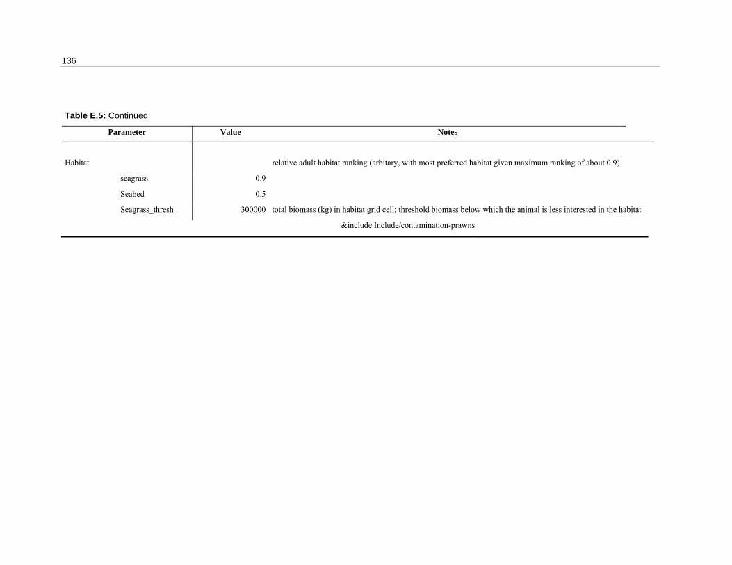
136
Table E.5: Continued
Parameter Value Notes
Habitat relative adult habitat ranking (arbitary, with most preferred habitat given maximum ranking of about 0.9)
seagrass 0.9
Seabed 0.5
Seagrass_thresh 300000 total biomass (kg) in habitat grid cell; threshold biomass below which the animal is less interested in the habitat
&include Include/contamination-prawns
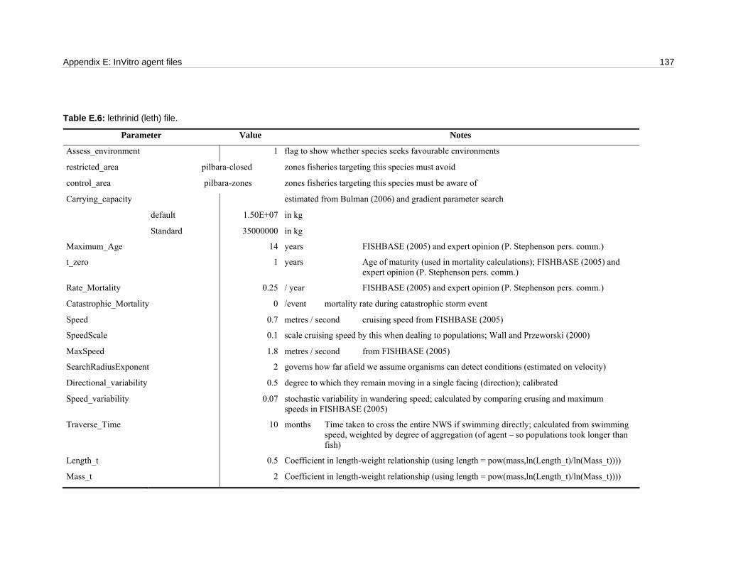
Appendix E: InVitro agent files 137
Table E.6: lethrinid (leth) file.
Parameter Value Notes
Assess_environment 1 flag to show whether species seeks favourable environments
restricted_area pilbara-closed zones fisheries targeting this species must avoid
control_area pilbara-zones zones fisheries targeting this species must be aware of
Carrying_capacity estimated from Bulman (2006) and gradient parameter search
default 1.50E+07 in kg
Standard 35000000 in kg
Maximum_Age 14 years FISHBASE (2005) and expert opinion (P. Stephenson pers. comm.)
t_zero 1 years Age of maturity (used in mortality calculations); FISHBASE (2005) and expert opinion (P. Stephenson pers. comm.)
Rate_Mortality 0.25 / year FISHBASE (2005) and expert opinion (P. Stephenson pers. comm.)
Catastrophic_Mortality 0 /event mortality rate during catastrophic storm event
Speed 0.7 metres / second cruising speed from FISHBASE (2005)
SpeedScale 0.1 scale cruising speed by this when dealing to populations; Wall and Przeworski (2000)
MaxSpeed 1.8 metres / second from FISHBASE (2005)
SearchRadiusExponent 2 governs how far afield we assume organisms can detect conditions (estimated on velocity)
Directional_variability 0.5 degree to which they remain moving in a single facing (direction); calibrated
Speed_variability 0.07 stochastic variability in wandering speed; calculated by comparing crusing and maximum speeds in FISHBASE (2005)
Traverse_Time 10 months Time taken to cross the entire NWS if swimming directly; calculated from swimming speed, weighted by degree of aggregation (of agent – so populations took longer than fish)
Length_t 0.5 Coefficient in length-weight relationship (using length = pow(mass,ln(Length_t)/ln(Mass_t))))
Mass_t 2 Coefficient in length-weight relationship (using length = pow(mass,ln(Length_t)/ln(Mass_t))))

138
Table E.6: Continued
Parameter Value Notes
Width_a 0.1 dimensions of organism; directly measured
Width_b 0.17 dimensions of organism; directly measured
Gape/Width 0.9 ratio of gape to width (estimated from direct measurements)
Capacity 0.3 gut capacity as a proportion of length (estimate from direct measurements)
Metabolism 0 kg of food burned per second determines if organisms must hunt or we assume adequate food (later assumed for MSE runs here)
propMale 0.5 proportion male (from WA fisheries stock assessments, P. Stephenson 2003)
Mlinf 31.52 male asymptotic maximum length; from FISHBASE (2005) and expert opinion (P. Stephenson pers. comm.)
Mlength_lambda 0.716 years; male parameter used in age-mass relationship (growth equation); from FISHBASE (2005) and expert opinion (P. Stephenson pers. comm.)
Mvbt0 -0.472 male Von Bertalanfy to; FISHBASE (2005) and expert opinion (P. Stephenson pers. comm.)
MlengthA 1.28E-08 male length-weight coefficient; FISHBASE (2005) and expert opinion (P. Stephenson pers. comm.)
MlengthB 3.0881 male length-weight exponent; FISHBASE (2005) and expert opinion (P. Stephenson pers. comm.)
Flinf 29.31 female asymptotic maximum length; from FISHBASE (2005) and expert opinion (P. Stephenson pers. comm.)
Flength_lambda 0.742 years; female parameter used in age-mass relationship (growth equation); from FISHBASE (2005) and expert opinion (P. Stephenson pers. comm.)
Fvbt0 -0.471 female Von Bertalanfy to; FISHBASE (2005) and expert opinion (P. Stephenson pers. comm.)
FlengthA 1.29E-08 female length-weight coefficient; FISHBASE (2005) and expert opinion (P. Stephenson pers. comm.)
FlengthB 3.0881 female length-weight exponent; FISHBASE (2005) and expert opinion (P. Stephenson pers. comm.)
Safe_Range 6 six times the cruising speed estimated from visibility ranges; not used when adequate food assumed
Perception_Range 20 times the cruising speed range at which prey may be detected
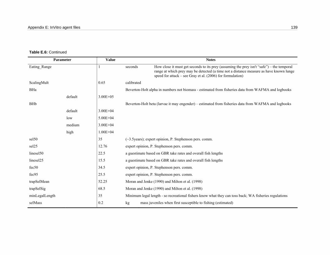
Appendix E: InVitro agent files 139
Table E.6: Continued
Parameter Value Notes
Eating_Range 1 seconds How close it must get seconds to its prey (assuming the prey isn't “safe”) – the temporal range at which prey may be detected (a time not a distance measure as have known lunge speed for attack – see Gray et al. (2006) for formulation)
ScalingMult 0.65 calibrated
BHa Beverton-Holt alpha in numbers not biomass - estimated from fisheries data from WAFMA and logbooks
default 3.00E+05
BHb Beverton-Holt beta (larvae it may engender) – estimated from fisheries data from WAFMA and logbooks
default 3.00E+04
low 5.00E+04
medium 3.00E+04
high 1.00E+04
sel50 35 (~3.5years); expert opinion, P. Stephenson pers. comm.
sel25 12.76 expert opinion, P. Stephenson pers. comm.
linesel50 22.5 a guestimate based on GBR take rates and overall fish lengths
linesel25 15.5 a guestimate based on GBR take rates and overall fish lengths
fec50 34.5 expert opinion, P. Stephenson pers. comm.
fec95 25.5 expert opinion, P. Stephenson pers. comm.
trapSelMean 52.25 Moran and Jenke (1990) and Milton et al. (1998)
trapSelSig 68.5 Moran and Jenke (1990) and Milton et al. (1998)
minLegalLength 35 Minimum legal length - so recreational fishers know what they can toss back; WA fisheries regulations
selMass 0.2 kg mass juveniles when first susceptible to fishing (estimated)

140
Table E.6: Continued
Parameter Value Notes
spatialCatchFactor estimated from fisheries data from WAFMA and logbooks (to minimise differences between observed and predicted trawl catches)
default 1.00E-02
spatialTrapCatchFactor estimated from fisheries data from WAFMA and logbooks (to minimise differences between observed and predicted trap catches)
default 1.00E-02
numberParms 4 number of parms to estimate in stock assessment (if performed for this species)
Max_mass 8.5 kg Upper limit of mass; Kailola et al. (1993) and FISHBASE (2005)
mass_lambda 0.03 specified in years; for age-mass equation (tuned to give realistic age spans given known masses)
spatialLarvalFactor 1E-11 calibrated to give a plausible stock-recruit relationship
Fecundity 1000000 how many larvae it may engender - if fish agent not population agent; from Kailola et al. (1993)
Breeding
age week*208 breeding age; from Kailola et al. (1993)
Start week*17 start time of first cycle after the start of the Julian year; from Kailola et al. (1993)
offset 0 allows for continuous breeding – not needed for this species
Period year time between individual breeding seasons; Kailola et al. (1993)
fallow_period 0 time time between breeding events; from Kailola et al. (1993)
Group_Size program control parameter – dictates maximum school size (above this the school splits)
default 7.00E+05 size of groups ( dictates distributions in schools; calibration parameter (only used in fine scale simulations during development, not regional scale MSE))
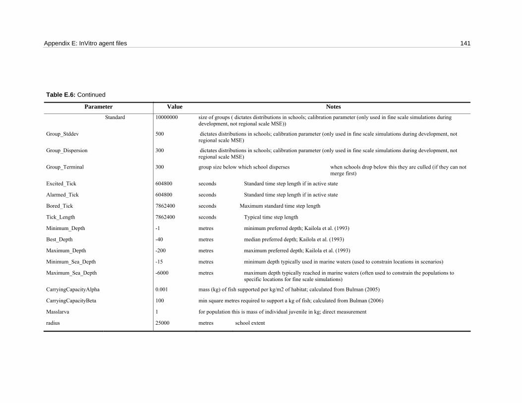
Appendix E: InVitro agent files 141
Table E.6: Continued
Parameter Value Notes
Standard 10000000 size of groups ( dictates distributions in schools; calibration parameter (only used in fine scale simulations during development, not regional scale MSE))
Group_Stddev 500 dictates distributions in schools; calibration parameter (only used in fine scale simulations during development, not regional scale MSE)
Group_Dispersion 300 dictates distributions in schools; calibration parameter (only used in fine scale simulations during development, not regional scale MSE)
Group_Terminal 300 group size below which school disperses when schools drop below this they are culled (if they can not merge first)
Excited_Tick 604800 seconds Standard time step length if in active state
Alarmed_Tick 604800 seconds Standard time step length if in active state
Bored_Tick 7862400 seconds Maximum standard time step length
Tick_Length 7862400 seconds Typical time step length
Minimum_Depth -1 metres minimum preferred depth; Kailola et al. (1993)
Best_Depth -40 metres median preferred depth; Kailola et al. (1993)
Maximum_Depth -200 metres maximum preferred depth; Kailola et al. (1993)
Minimum_Sea_Depth -15 metres minimum depth typically used in marine waters (used to constrain locations in scenarios)
Maximum_Sea_Depth -6000 metres maximum depth typically reached in marine waters (often used to constrain the populations to specific locations for fine scale simulations)
CarryingCapacityAlpha 0.001 mass (kg) of fish supported per kg/m2 of habitat; calculated from Bulman (2005)
CarryingCapacityBeta 100 min square metres required to support a kg of fish; calculated from Bulman (2006)
Masslarva 1 for population this is mass of individual juvenile in kg; direct measurement
radius 25000 metres school extent

142
Table E.6: Continued
Parameter Value Notes
trawl_efficiency 0.1 efficiency of trawlers against species on juvenile stages (expert opinion; P. Stephenson pers. comm.)
assess_environment 1 flag to show whether species seeks favourable environments
Awareness_type 1 0 for fine scale awareness, 1 for large scale program control parameter – dictating resolution of adviser agent interrogation (see Gray et al. (2006))
ScalingBestSeaDepth 0.0001 Weighting for influence of preferred depth in guiding habitat selection
Larva Juvenile parameters
tick_length 7862400 seconds Typical time step length for juvenile age phases
bored_tick 7862400 seconds Maximum standard time step length for juvenile age stages
alarmed_tick 600 seconds Standard time step length if in active state for juvenile age stages
suppress_wander 1 Prevents blastula wandering from original position
head_for 1 flag setting whether they head for random spot or closest when recruiting or settling: (1 for heading for closest, 0 for heading for random)
trawl_efficiency 0 efficiency of trawlers against juvenile age stages (expert opinion, Keith Sainsbury CSIRO pers. comm.)
projection_efficiency_scalar 1 scalar on fishing efficiency so no discontinuity from historical to projection treatement (given different spatial scales of operation)
radius 25000 metres Radius of juvenile patch / school (calibrated to give credible juvenile dynamics)
spatialLarvalFactor 1E-11 settlement “stock-recruit” relationship scalar – calibrated to give plausible overall stock-recruit relationship
First Parameters for first age phase of larval agents
tracer_minor 3 flag to indicate form of advection used (3 means vertices are advected)
Current_K 0.4 metres / second coefficient for movement of unsettled larva with currents; calibrated so that observed time from spawning to settlement obtained and correct movement patterns seen
Wind_K 0.1 metres / second coefficient for movement of unsettled larva with winds; calibrated so that observed time from spawning to settlement obtained and correct movement patterns seen
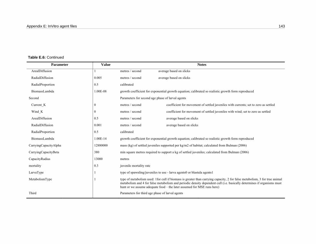
Appendix E: InVitro agent files 143
Table E.6: Continued
Parameter Value Notes
ArealDiffusion 1 metres / second average based on slicks
RadialDiffusion 0.005 metres / second average based on slicks
RadialProportion 0.5 calibrated
BiomassLambda 1.00E-08 growth coefficient for exponential growth equation; calibrated so realistic growth form reproduced
Second Parameters for second age phase of larval agents
Current_K 0 metres / second coefficient for movement of settled juveniles with currents; set to zero as settled
Wind_K 0 metres / second coefficient for movement of settled juveniles with wind; set to zero as settled
ArealDiffusion 0.5 metres / second average based on slicks
RadialDiffusion 0.001 metres / second average based on slicks
RadialProportion 0.5 calibrated
BiomassLambda 1.00E-14 growth coefficient for exponential growth equation; calibrated so realistic growth form reproduced
CarryingCapacityAlpha 12880000 mass (kg) of settled juveniles supported per kg/m2 of habitat; calculated from Bulman (2006)
CarryingCapacityBeta 380 min square metres required to support a kg of settled juveniles; calculated from Bulman (2006)
CapacityRadius 13000 metres
mortality 0.3 juvenile mortality rate
LarvaType 1 type of spawnling/juveniles to use - larva agents0 or blastula agents1
MetabolismType 1 type of metabolism used: 1for cull if biomass is greater than carrying capacity, 2 for false metabolism, 3 for true animal metabolism and 4 for false metabolism and periodic density dependent cull (i.e. basically determines if organisms must hunt or we assume adequate food – the later assumed for MSE runs here)
Third Parameters for third age phase of larval agents

144
Table E.6: Continued
Parameter Value Notes
Current_K 1 metres / second coefficient for movement of unsettled larva with currents; calibrated so that observed movement patterns are reproduced
Wind_K 0 metres / second coefficient for movement of unsettled larva with winds; set to zero as directed movement
Settling
age 31449600 age when begin settling; Kailola et al. (1993)
radius 200000 distance from centre of bed of suitable habitat type that will settle
scale 0.5 scalar on habitat quality for settling
offset 1 offset on habitat quality for settling
habitat sponge identifies suitable settling habitat
habitat_type 4 habitat agent type (1 for data grid in file, 2 for habitat tracer agents, 3 for polyorganism agents, 4 for benthic agents, 5 for no agent type set and 6 for carrying capacity dependent settlement)
direction_travel -1 identifies whether swimming on-shore (1) or offshore (-1) or whereever (0) at this life stage
Recruitment
age 31622400 age when begin recruiting to adult population; Kailola et al. (1993)
temporal_radius 604800 seconds; time in blastula queue when “close enough” to recruit; calibrated to give realistic settlement patterns
radius 10000 distance from centre of bed of suitable habitat type that will recruit
scale 0.5 scalar on recruitment habitat preferences
offset 1 offset on recruitment habitat quality
habitat sponge identifies suitable recruiting habitat
habitat_type 4 habitat agent type (1 for data grid in file, 2 for habitat tracer agents, 3 for polyorganism agents, 4 for benthic agents, 5 for no agent type set and 6 for carrying capacity dependent recruitment)

Appendix E: InVitro agent files 145
Table E.6: Continued
Parameter Value Notes
direction_travel -1 identifies whether swimming on-shore (1) or offshore (-1) or whereever (0) at this life stage
Mass0 0.05 kg UNUSED
aggregate_rate 1 rate of polygon contraction when recruiting; calibrated to give smooth transition
Prefers relative prey ranking (arbitary, with main prey given maximum ranking of about 0.9)
benthos 0.9
fish 0.05
bycatch 0.1
Fears relative fear ranking (arbitary, with main predators given maximum ranking of about 0.9)
Tuna 0.9
Shark 0.9
Habitat relative adult habitat ranking (arbitary, with most preferred habitat given maximum ranking of about 0.9)
sponge 0.7
self 0.01 If prefer/detest to be with conspecifics then include them in the preferred habitat definition
Sponge_thresh 160000 total biomass (kg) in habitat grid cell; threshold biomass below which the animal is less interested in the habitat
self_thresh 350000 total biomass (kg) in habitat grid cell; threshold biomass below which density of conspecifics is insufficient to act as a true attractant/repellant
self_scalar -10 If < 1 then find high density of conspecifics a repellant
&include Include/contamination-finfish
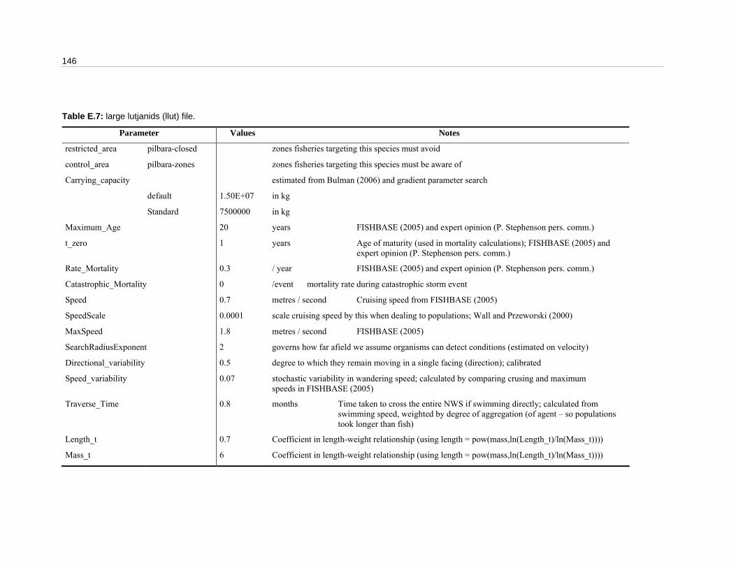
146
Table E.7: large lutjanids (llut) file.
Parameter Values Notes
restricted_area pilbara-closed zones fisheries targeting this species must avoid
control_area pilbara-zones zones fisheries targeting this species must be aware of
Carrying_capacity estimated from Bulman (2006) and gradient parameter search
default 1.50E+07 in kg
Standard 7500000 in kg
Maximum_Age 20 years FISHBASE (2005) and expert opinion (P. Stephenson pers. comm.)
t_zero 1 years Age of maturity (used in mortality calculations); FISHBASE (2005) and expert opinion (P. Stephenson pers. comm.)
Rate_Mortality 0.3 / year FISHBASE (2005) and expert opinion (P. Stephenson pers. comm.)
Catastrophic_Mortality 0 /event mortality rate during catastrophic storm event
Speed 0.7 metres / second Cruising speed from FISHBASE (2005)
SpeedScale 0.0001 scale cruising speed by this when dealing to populations; Wall and Przeworski (2000)
MaxSpeed 1.8 metres / second FISHBASE (2005)
SearchRadiusExponent 2 governs how far afield we assume organisms can detect conditions (estimated on velocity)
Directional_variability 0.5 degree to which they remain moving in a single facing (direction); calibrated
Speed_variability 0.07 stochastic variability in wandering speed; calculated by comparing crusing and maximum speeds in FISHBASE (2005)
Traverse_Time 0.8 months Time taken to cross the entire NWS if swimming directly; calculated from swimming speed, weighted by degree of aggregation (of agent – so populations took longer than fish)
Length_t 0.7 Coefficient in length-weight relationship (using length = pow(mass,ln(Length_t)/ln(Mass_t))))
Mass_t 6 Coefficient in length-weight relationship (using length = pow(mass,ln(Length_t)/ln(Mass_t))))
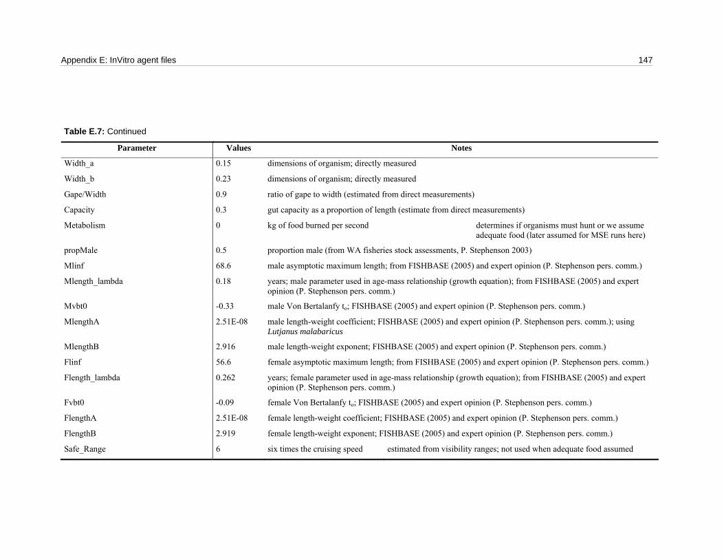
Appendix E: InVitro agent files 147
Table E.7: Continued
Parameter Values Notes
Width_a 0.15 dimensions of organism; directly measured
Width_b 0.23 dimensions of organism; directly measured
Gape/Width 0.9 ratio of gape to width (estimated from direct measurements)
Capacity 0.3 gut capacity as a proportion of length (estimate from direct measurements)
Metabolism 0 kg of food burned per second determines if organisms must hunt or we assume adequate food (later assumed for MSE runs here)
propMale 0.5 proportion male (from WA fisheries stock assessments, P. Stephenson 2003)
Mlinf 68.6 male asymptotic maximum length; from FISHBASE (2005) and expert opinion (P. Stephenson pers. comm.)
Mlength_lambda 0.18 years; male parameter used in age-mass relationship (growth equation); from FISHBASE (2005) and expert opinion (P. Stephenson pers. comm.)
Mvbt0 -0.33 male Von Bertalanfy to; FISHBASE (2005) and expert opinion (P. Stephenson pers. comm.)
MlengthA 2.51E-08 male length-weight coefficient; FISHBASE (2005) and expert opinion (P. Stephenson pers. comm.); using Lutjanus malabaricus
MlengthB 2.916 male length-weight exponent; FISHBASE (2005) and expert opinion (P. Stephenson pers. comm.)
Flinf 56.6 female asymptotic maximum length; from FISHBASE (2005) and expert opinion (P. Stephenson pers. comm.)
Flength_lambda 0.262 years; female parameter used in age-mass relationship (growth equation); from FISHBASE (2005) and expert opinion (P. Stephenson pers. comm.)
Fvbt0 -0.09 female Von Bertalanfy to; FISHBASE (2005) and expert opinion (P. Stephenson pers. comm.)
FlengthA 2.51E-08 female length-weight coefficient; FISHBASE (2005) and expert opinion (P. Stephenson pers. comm.)
FlengthB 2.919 female length-weight exponent; FISHBASE (2005) and expert opinion (P. Stephenson pers. comm.)
Safe_Range 6 six times the cruising speed estimated from visibility ranges; not used when adequate food assumed

148
Table E.7: Continued
Parameter Values Notes
Perception_Range 20 times the cruising speed range at which prey is detected
Eating_Range 1 seconds How close it must get seconds to it's prey (assuming the prey isn't “safe”) – the temporal range at which prey may be detected (a time not a distance measure as have known lunge speed for attack – see Gray et al. (2006) for formulation)
ScalingMult 1 calibrated
BHa Beverton-Holt alpha in numbers not biomass - estimated from fisheries data from WAFMA and logbooks
default 3.00E+04
BHb Beverton-Holt beta (larvae it may engender) – estimated from fisheries data from WAFMA and logbooks
default 5.00E+03
low 1.00E+04
medium 5.00E+03
high 1.00E+02
sel50 38.5 (~3.5years); expert opinion, P. Stephenson pers. comm.
sel25 34.21 expert opinion, P. Stephenson pers. comm.
linesel50 32.5 using coral trout selectivity (Fulton et al. 1999)
linesel25 30.5 using coral trout selectivity (Fulton et al. 1999)
fec50 38.5 expert opinion, P. Stephenson pers. comm.
fec95 42 expert opinion, P. Stephenson pers. comm.
trapSelMean 52.25 Moran and Jenke (1990) and Milton et al.(1998)
trapSelSig 68.5 Moran and Jenke (1990) and Milton et al. (1998)
minLegalLength 41 Minimum legal length - so recreational fishers know what they can toss back; WA fisheries regulations
selMass 0.2 kg mass juveniles when first susceptible to fishing (estimated)

Appendix E: InVitro agent files 149
Table E.7: Continued
Parameter Values Notes
spatialCatchFactor estimated from fisheries data from WAFMA and logbooks (to minimise differences between observed and predicted trawl catches)
default 1.00E-02
spatialTrapCatchFactor
estimated from fisheries data from WAFMA and logbooks (to minimise differences between observed and predicted trap catches)
Default 1.00E-02
numberParms 4 number of parms to estimate in stock assessment (if performed for this species)
Max_mass 8.4 kg Upper limit of mass; Kailola et al. (1993) and and FISHBASE (2005)
mass_lambda 0.03 years; male parameter used in age-mass relationship (growth equation); from FISHBASE (2005) and expert opinion (P. Stephenson pers. comm.)
spatialLarvalFactor 1E-11 calibrated to give a plausible stock-recruit relationship
Fecundity 100000 how many larvae it may engender – if fish agent not population agent; from Kailola et al. (1993)
Breeding
age week*208 breeding age; from Kailola et al. (1993)
start week*39 start time of first cycle after the start of the Julian year; from Kailola et al. (1993)
offset 0 allows for continuous breeding – not needed for this species
period year time between individual breeding seasons; Kailola et al. (1993)
fallow_period 0 time time between breeding events; from Kailola et al. (1993)
Group_Size program control parameter – dictates maximum school size (above this the school splits)

150
Table E.7: Continued
Parameter Values Notes
default 1.00E+05 size of groups ( dictates distributions in schools; calibration parameter (only used in fine scale simulations during development, not regional scale MSE))
Standard 100000 size of groups ( dictates distributions in schools; calibration parameter (only used in fine scale simulations during development, not regional scale MSE)) (500000)
Group_Stddev 500 dictates distributions in schools; calibration parameter (only used in fine scale simulations during development, not regional scale MSE)
Group_Dispersion 300 dictates distributions in schools; calibration parameter (only used in fine scale simulations during development, not regional scale MSE)
Group_Terminal 300 group size below which school disperses when schools drop below this they are culled (if they can not merge first)
Excited_Tick 604800 seconds Standard time step length if in active state
Alarmed_Tick 604800 seconds Standard time step length if in active state
Bored_Tick 7862400 seconds Maximum standard time step length
Tick_Length 7862400 seconds Typical time step length
Minimum_Depth -1 metres minimum preferred depth; Kailola et al. (1993)
Best_Depth -90 metres median preferred depth; Kailola et al. (1993)
Maximum_Depth -200 metres maximum preferred depth; Kailola et al. (1993)
Minimum_Sea_Depth -15 metres minimum depth typically used in marine waters (used to constrain locations in scenarios)
Maximum_Sea_Depth -6000 metres maximum depth typically reached in marine waters (often used to constrain the populations to specific locations for fine scale simulations)
CarryingCapacityAlpha 0.005 mass (kg) of fish supported per kg/m2 of habitat; calculated from Bulman (2006)
CarryingCapacityBeta 200 min square metres required to support a kg of fish; calculated from Bulman (2006)

Appendix E: InVitro agent files 151
Table E.7: Continued
Parameter Values Notes
Masslarva 1 for population this is mass of individual juvenile in kg; direct measurement
radius 25000 metres school extent
trawl_efficiency 0.1 efficiency of trawlers against species on juvenile stages (expert opinion; P. Stephenson pers. comm.)
assess_environment 1 flag to show whether species seeks favourable environments
Awareness_type 1 0 for fine scale awareness, 1 for large scale program control parameter – dictating resolution of adviser agent interrogation (see Gray et al. (2006))
ScalingBestSeaDepth
default 0.0001 Weighting for influence of preferred depth in guiding habitat selection
Larva Juvenile parameters
tick_length 7862400 seconds Typical time step length for juvenile age stages
bored_tick 7862400 seconds Maximum standard time step length for juvenile age stages
alarmed_tick 600 seconds Standard time step length if in active state for juvenile age stages
suppress_wander 1 Prevents blastula wandering from original position
head_for 1 flag setting whether they head for random spot or closest when recruiting or settling: (1 for heading for closest, 0 for heading for random)
trawl_efficiency 0 efficiency of trawlers against juvenile age stages (expert opinion, Keith Sainsbury CSIRO pers. comm.)
projection_efficiency_scalar 1 scalar on fishing efficiency so no discontinuity from historical to projection treatement (given different spatial scales of operation)
radius 25000 metres Radius of juvenile patch / school (calibrated to give credible juvenile dynamics)
spatialLarvalFactor 1E-11 settlement “stock-recruit” relationship scalar – calibrated to give plausible overall stock-recruit relationship
First Parameters for first age phase of larval agents
tracer_minor 3 flag to indicate form of advection used (3 means vertices are advected)

152
Table E.7: Continued
Parameter Values Notes Current_K 0.4 metres / second coefficient for movement of unsettled larva with currents; calibrated so that observed time from spawning to
settlement obtained and correct movement patterns seen
Wind_K 0.1 metres / second coefficient for movement of unsettled larva with winds; calibrated so that observed time from spawning to settlement obtained and correct movement patterns seen
ArealDiffusion 1 metres / second average based on slicks
RadialDiffusion 0.005 metres / second average based on slicks
RadialProportion 0.5 calibrated
BiomassLambda 1.00E-08 growth coefficient for exponential growth equation; calibrated so realistic growth form reproduced
Second Parameters for second age phase of larval agents
Current_K 0 metres / second coefficient for movement of settled juveniles with currents; set to zero as settled
Wind_K 0 metres / second coefficient for movement of settled juveniles with wind; set to zero as settled
ArealDiffusion 0.5 metres / second average based on slicks
RadialDiffusion 0.001 metres / second average based on slicks
RadialProportion 0.5 unused
BiomassLambda 1.00E-14 growth coefficient for exponential growth equation; calibrated so realistic growth form reproduced
CarryingCapacityAlpha 2.23E+08 mass (kg) of settled juveniles supported per kg/m2 of habitat; calculated from Bulman (2006)
CarryingCapacityBeta 380 min square metres required to support a kg of settled juveniles; calculated from Bulman (2006)
CapacityRadius 13000 metres
mortality 0.35 juvenile mortality rate
LarvaType 1 type of spawnling/juveniles to use – larva agents0 or blastula agents1
MetabolismType 1 type of metabolism used: 1for cull if biomass is greater than carrying capacity, 2 for false metabolism, 3 for true animal metabolism and 4 for false metabolism and periodic density dependent cull (i.e. basically determines if organisms must hunt or we assume adequate food – the later assumed for MSE runs here)

Appendix E: InVitro agent files 153
Table E.7: Continued
Parameter Values Notes
Third Parameters for third age phase of larval agents
Current_K 1 metres / second coefficient for movement of unsettled larva with currents; calibrated so that observed movement patterns are reproduced
Wind_K 0 metres / second coefficient for movement of unsettled larva with winds; set to zero as directed movement
Settling
age 15724800 age when begin settling; Kailola et al. (1993)
radius 10000 distance from centre of bed of suitable habitat type that will settle
scale 0.5 scalar on habitat quality for settling
offset 1 offset on habitat quality for settling
habitat sponge identifies suitable settling habitat
habitat_type 4 habitat agent type (1 for data grid in file, 2 for habitat tracer agents, 3 for polyorganism agents, 4 for benthic agents, 5 for no agent type set and 6 for carrying capacity dependent settlement)
direction_travel 0 identifies whether swimming on-shore (1) or offshore (-1) or whereever (0) at this life stage
Recruitment
age 31622400 age when begin recruiting to adult population; Kailola et al. (1993)
temporal_radius 604800 seconds; time in blastula queue when “close enough” to recruit; calibrated to give realistic settlement patterns
radius 10000 distance from centre of bed of suitable habitat type that will recruit
scale 0.5 scalar on recruitment habitat preferences
offset 1 offset on recruitment habitat quality
habitat sponge identifies suitable recruiting habitat
habitat_type 4 habitat agent type (1 for data grid in file, 2 for habitat tracer agents, 3 for polyorganism agents, 4 for benthic agents, 5 for no agent type set and 6 for carrying capacity dependent recruitment)
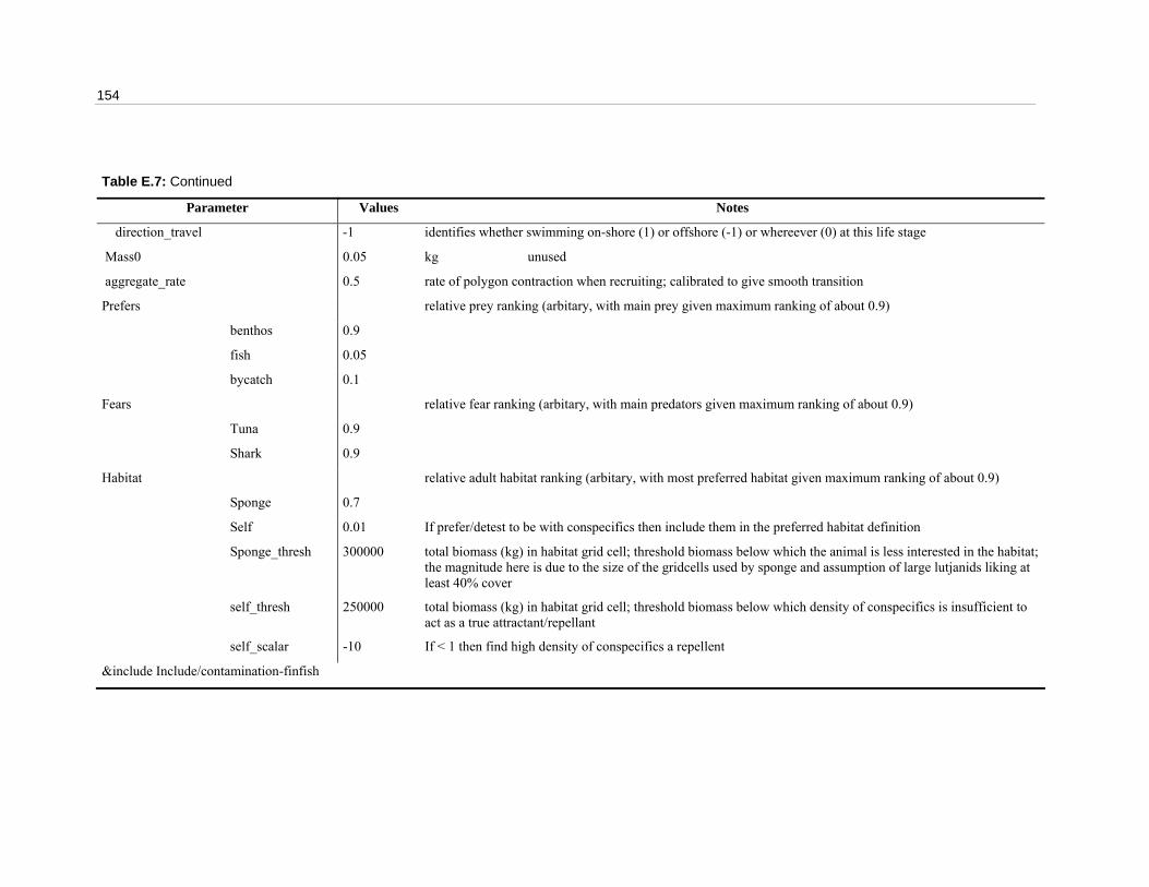
154
Table E.7: Continued
Parameter Values Notes
direction_travel -1 identifies whether swimming on-shore (1) or offshore (-1) or whereever (0) at this life stage
Mass0 0.05 kg unused
aggregate_rate 0.5 rate of polygon contraction when recruiting; calibrated to give smooth transition
Prefers relative prey ranking (arbitary, with main prey given maximum ranking of about 0.9)
benthos 0.9
fish 0.05
bycatch 0.1
Fears relative fear ranking (arbitary, with main predators given maximum ranking of about 0.9)
Tuna 0.9
Shark 0.9
Habitat relative adult habitat ranking (arbitary, with most preferred habitat given maximum ranking of about 0.9)
Sponge 0.7
Self 0.01 If prefer/detest to be with conspecifics then include them in the preferred habitat definition
Sponge_thresh 300000 total biomass (kg) in habitat grid cell; threshold biomass below which the animal is less interested in the habitat; the magnitude here is due to the size of the gridcells used by sponge and assumption of large lutjanids liking at least 40% cover
self_thresh 250000 total biomass (kg) in habitat grid cell; threshold biomass below which density of conspecifics is insufficient to act as a true attractant/repellant
self_scalar -10 If < 1 then find high density of conspecifics a repellent
&include Include/contamination-finfish

Appendix E: InVitro agent files 155
Table E.8: Lutjanus sebae (lsebae) file.
Parameter Values Notes
restricted_area pilbara-closed zones fisheries targeting this species must avoid
control_area pilbara-zones zones fisheries targeting this species must be aware of
Carrying_capacity estimated from Bulman (2006) and gradient parameter search
default 1.50E+07 in kg
Standard 6000000 in kg
Maximum_Age 25 years FISHBASE (2005) and expert opinion (P. Stephenson pers. comm.)
t_zero 1 years Age of maturity (used in mortality calculations); FISHBASE (2005) and expert opinion (P. Stephenson pers. comm.)
Rate_Mortality 0.13 / year FISHBASE (2005) and expert opinion (P. Stephenson pers. comm.)
Catastrophic_Mortality 0 / event mortality rate during catastrophic storm event
Speed 0.7 metres / second cruising speed from FISHBASE (2005)
SpeedScale 0.0001 scale cruising speed by this when dealing to populations; Wall and Przeworski (2000)
MaxSpeed 1.8
SearchRadiusExponent 2 governs how far afield we assume organisms can detect conditions (estimated on velocity)
Directional_variability 0.5 degree to which they remain moving in a single facing (direction); calibrated
Speed_variability 0.07 stochastic variability in wandering speed; calculated by comparing crusing and maximum speeds in FISHBASE (2005)
Traverse_Time 10 months Time taken to cross the entire NWS if swimming directly; calculated from swimming speed, weighted by degree of aggregation (of agent – so populations took longer than fish)
Length_t 0.7 Coefficient in length-weight relationship (using length = pow(mass,ln(Length_t)/ln(Mass_t))))
Mass_t 6 Coefficient in length-weight relationship (using length = pow(mass,ln(Length_t)/ln(Mass_t))))
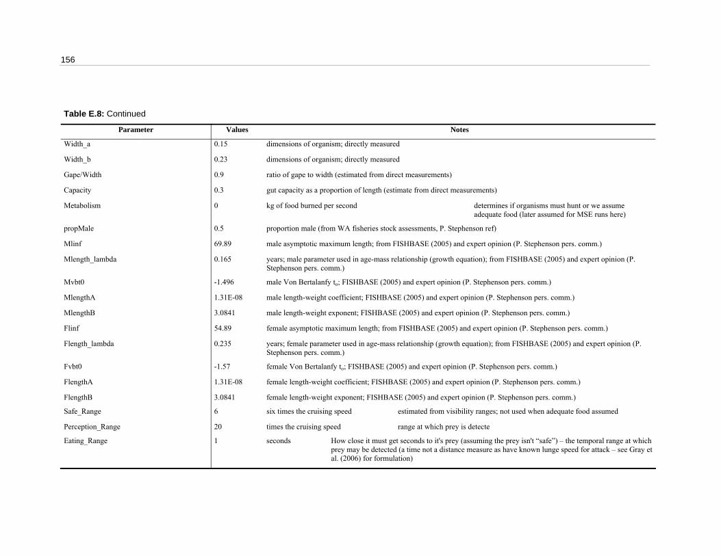
156
Table E.8: Continued
Parameter Values Notes
Width_a 0.15 dimensions of organism; directly measured
Width_b 0.23 dimensions of organism; directly measured
Gape/Width 0.9 ratio of gape to width (estimated from direct measurements)
Capacity 0.3 gut capacity as a proportion of length (estimate from direct measurements)
Metabolism 0 kg of food burned per second determines if organisms must hunt or we assume adequate food (later assumed for MSE runs here)
propMale 0.5 proportion male (from WA fisheries stock assessments, P. Stephenson ref)
Mlinf 69.89 male asymptotic maximum length; from FISHBASE (2005) and expert opinion (P. Stephenson pers. comm.)
Mlength_lambda 0.165 years; male parameter used in age-mass relationship (growth equation); from FISHBASE (2005) and expert opinion (P. Stephenson pers. comm.)
Mvbt0 -1.496 male Von Bertalanfy to; FISHBASE (2005) and expert opinion (P. Stephenson pers. comm.)
MlengthA 1.31E-08 male length-weight coefficient; FISHBASE (2005) and expert opinion (P. Stephenson pers. comm.)
MlengthB 3.0841 male length-weight exponent; FISHBASE (2005) and expert opinion (P. Stephenson pers. comm.)
Flinf 54.89 female asymptotic maximum length; from FISHBASE (2005) and expert opinion (P. Stephenson pers. comm.)
Flength_lambda 0.235 years; female parameter used in age-mass relationship (growth equation); from FISHBASE (2005) and expert opinion (P. Stephenson pers. comm.)
Fvbt0 -1.57 female Von Bertalanfy to; FISHBASE (2005) and expert opinion (P. Stephenson pers. comm.)
FlengthA 1.31E-08 female length-weight coefficient; FISHBASE (2005) and expert opinion (P. Stephenson pers. comm.)
FlengthB 3.0841 female length-weight exponent; FISHBASE (2005) and expert opinion (P. Stephenson pers. comm.)
Safe_Range 6 six times the cruising speed estimated from visibility ranges; not used when adequate food assumed
Perception_Range 20 times the cruising speed range at which prey is detecte
Eating_Range 1 seconds How close it must get seconds to it's prey (assuming the prey isn't “safe”) – the temporal range at which prey may be detected (a time not a distance measure as have known lunge speed for attack – see Gray et al. (2006) for formulation)

Appendix E: InVitro agent files 157
Table E.8: Continued
Parameter Values Notes
ScalingMult 1 calibrated
BHa Beverton-Holt alpha in numbers not biomass - estimated from fisheries data from WAFMA and logbooks
default 3.00E+03
BHb Beverton-Holt beta (larvae it may engender) – estimated from fisheries data from WAFMA and logbooks
default 5.00E+03
Low 9.00E+03
medium 5.00E+03
High 1.00E+03
sel50 38.5 (~3.5years); expert opinion, P. Stephenson pers. comm.
sel25 34.21 (~3.5years); expert opinion, P. Stephenson pers. comm.
linesel50 30.5 using coral trout selectivity (Fulton et al. 1999) - adjusted down a little to reflect different sized fish
linesel25 28.5 using coral trout selectivity (Fulton et al. 1999) - adjusted down a little to reflect different sized fish
fec50 38.5 expert opinion, P. Stephenson pers. comm.
fec95 42 expert opinion, P. Stephenson pers. comm.
trapSelMean 52.25 Moran and Jenke (1990) and Milton et al. (1998)
trapSelSig 68.5 Moran and Jenke (1990) and Milton et al. (1998)
minLegalLength 41 Minimum legal length - so recreational fishers know what they can toss back; WA fisheries regulations (set same as for large lutjanids)
selMass 0.2 kg mass juveniles when first susceptible to fishing (estimated)
spatialCatchFactor estimated from fisheries data from WAFMA and logbooks (to minimise differences between observed and predicted trawl catches)
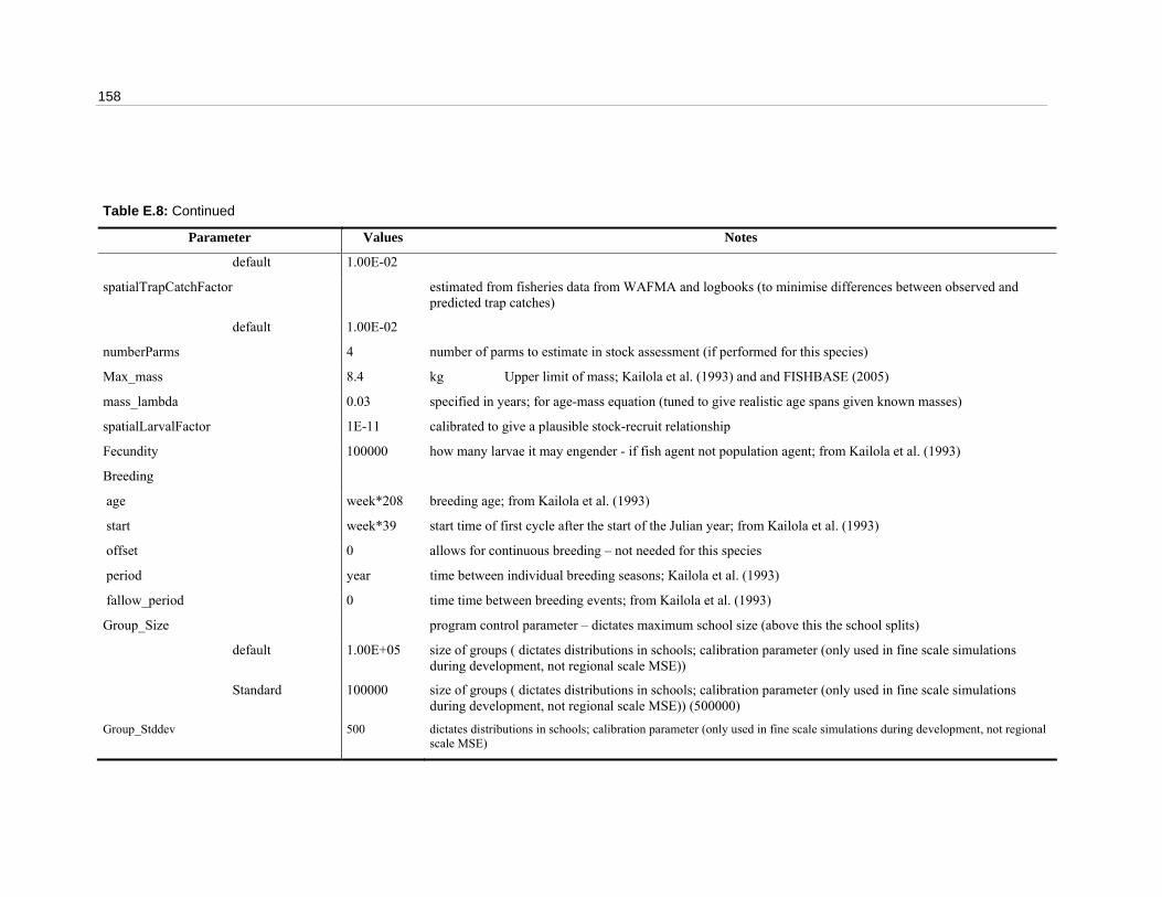
158
Table E.8: Continued
Parameter Values Notes
default 1.00E-02
spatialTrapCatchFactor estimated from fisheries data from WAFMA and logbooks (to minimise differences between observed and predicted trap catches)
default 1.00E-02
numberParms 4 number of parms to estimate in stock assessment (if performed for this species)
Max_mass 8.4 kg Upper limit of mass; Kailola et al. (1993) and and FISHBASE (2005)
mass_lambda 0.03 specified in years; for age-mass equation (tuned to give realistic age spans given known masses)
spatialLarvalFactor 1E-11 calibrated to give a plausible stock-recruit relationship
Fecundity 100000 how many larvae it may engender - if fish agent not population agent; from Kailola et al. (1993)
Breeding
age week*208 breeding age; from Kailola et al. (1993)
start week*39 start time of first cycle after the start of the Julian year; from Kailola et al. (1993)
offset 0 allows for continuous breeding – not needed for this species
period year time between individual breeding seasons; Kailola et al. (1993)
fallow_period 0 time time between breeding events; from Kailola et al. (1993)
Group_Size program control parameter – dictates maximum school size (above this the school splits)
default 1.00E+05 size of groups ( dictates distributions in schools; calibration parameter (only used in fine scale simulations during development, not regional scale MSE))
Standard 100000 size of groups ( dictates distributions in schools; calibration parameter (only used in fine scale simulations during development, not regional scale MSE)) (500000)
Group_Stddev 500 dictates distributions in schools; calibration parameter (only used in fine scale simulations during development, not regional scale MSE)
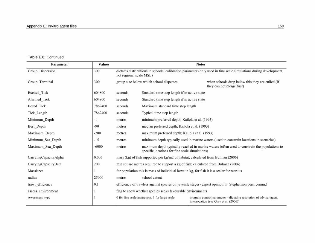
Appendix E: InVitro agent files 159
Table E.8: Continued
Parameter Values Notes
Group_Dispersion 300 dictates distributions in schools; calibration parameter (only used in fine scale simulations during development, not regional scale MSE)
Group_Terminal 300 group size below which school disperses when schools drop below this they are culled (if they can not merge first)
Excited_Tick 604800 seconds Standard time step length if in active state
Alarmed_Tick 604800 seconds Standard time step length if in active state
Bored_Tick 7862400 seconds Maximum standard time step length
Tick_Length 7862400 seconds Typical time step length
Minimum_Depth -1 metres minimum preferred depth; Kailola et al. (1993)
Best_Depth -90 metres median preferred depth; Kailola et al. (1993)
Maximum_Depth -200 metres maximum preferred depth; Kailola et al. (1993)
Minimum_Sea_Depth -15 metres minimum depth typically used in marine waters (used to constrain locations in scenarios)
Maximum_Sea_Depth -6000 metres maximum depth typically reached in marine waters (often used to constrain the populations to specific locations for fine scale simulations)
CarryingCapacityAlpha 0.005 mass (kg) of fish supported per kg/m2 of habitat; calculated from Bulman (2006)
CarryingCapacityBeta 200 min square metres required to support a kg of fish; calculated from Bulman (2006)
Masslarva 1 for population this is mass of individual larva in kg, for fish it is a scalar for recruits
radius 25000 metres school extent
trawl_efficiency 0.1 efficiency of trawlers against species on juvenile stages (expert opinion; P. Stephenson pers. comm.)
assess_environment 1 flag to show whether species seeks favourable environments
Awareness_type 1 0 for fine scale awareness, 1 for large scale program control parameter – dictating resolution of adviser agent interrogation (see Gray et al. (2006))

160
Table E.8: Continued
Parameter Values Notes
ScalingBestSeaDepth
default 0.0001 weighting for influence of preferred depth in guiding habitat selection
Larva juvenile parameters
tick_length 7862400 seconds Typical time step length for juvenile age stages
bored_tick 7862400 seconds Maximum standard time step length for juvenile age stages
alarmed_tick 600 seconds Standard time step length if in active state for juvenile age stages
suppress_wander 1 prevents blastula wandering from original position
head_for 1 flag setting whether they head for random spot or closest when recruiting or settling: (1 for heading for closest, 0 for heading for random)
trawl_efficiency 0 efficiency of trawlers against juvenile age phases (expert opinion, Keith Sainsbury CSIRO pers. comm.)
projection_efficiency_scalar 1 scalar on fishing efficiency so no discontinuity from historical to projection treatement (given different spatial scales of operation)
radius 25000 metres Radius of juvenile patch / school (calibrated to give credible juvenile dynamics)
spatialLarvalFactor 1E-11 settlement “stock-recruit” relationship scalar – calibrated to give plausible overall stock-recruit relationship
First parameters for first age phase of larval agents
tracer_minor 3 to advect centroid only, 3 to advect vertices
Current_K 0.4 metres / second coefficient for movement of unsettled larva with currents; calibrated so that observed time from spawning to settlement obtained and correct movement patterns seen
Wind_K 0.1 metres / second coefficient for movement of unsettled larva with winds; calibrated so that observed time from spawning to settlement obtained and correct movement patterns seen
ArealDiffusion 1 metres / second average based on slicks
RadialDiffusion 0.005 metres / second average based on slicks
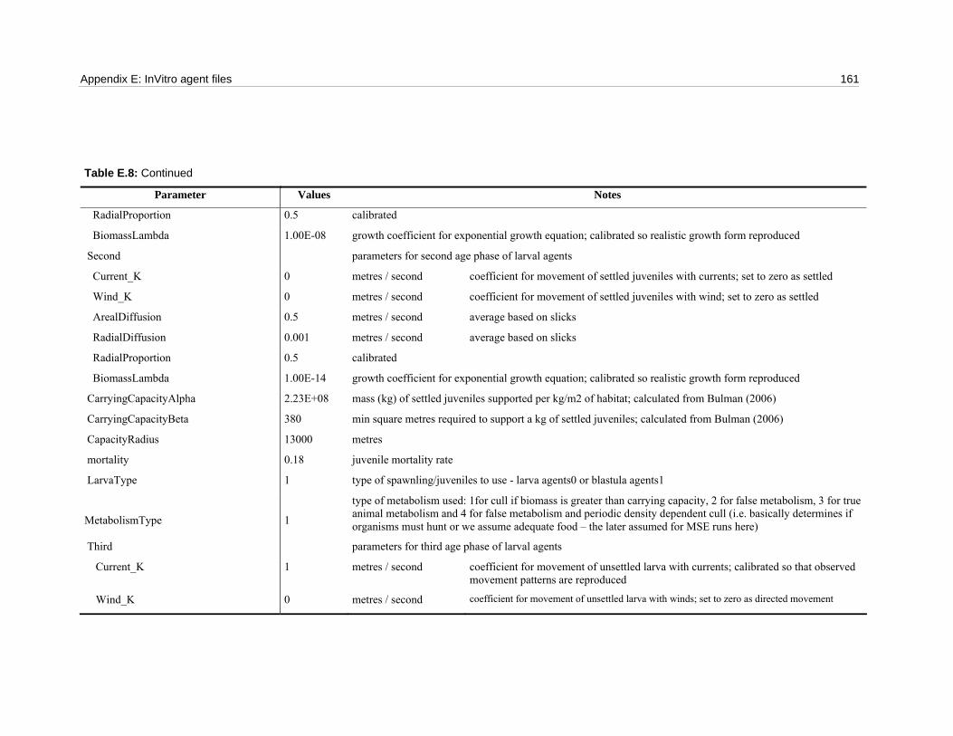
Appendix E: InVitro agent files 161
Table E.8: Continued
Parameter Values Notes
RadialProportion 0.5 calibrated
BiomassLambda 1.00E-08 growth coefficient for exponential growth equation; calibrated so realistic growth form reproduced
Second parameters for second age phase of larval agents
Current_K 0 metres / second coefficient for movement of settled juveniles with currents; set to zero as settled
Wind_K 0 metres / second coefficient for movement of settled juveniles with wind; set to zero as settled
ArealDiffusion 0.5 metres / second average based on slicks
RadialDiffusion 0.001 metres / second average based on slicks
RadialProportion 0.5 calibrated
BiomassLambda 1.00E-14 growth coefficient for exponential growth equation; calibrated so realistic growth form reproduced
CarryingCapacityAlpha 2.23E+08 mass (kg) of settled juveniles supported per kg/m2 of habitat; calculated from Bulman (2006)
CarryingCapacityBeta 380 min square metres required to support a kg of settled juveniles; calculated from Bulman (2006)
CapacityRadius 13000 metres
mortality 0.18 juvenile mortality rate
LarvaType 1 type of spawnling/juveniles to use - larva agents0 or blastula agents1
MetabolismType
1
type of metabolism used: 1for cull if biomass is greater than carrying capacity, 2 for false metabolism, 3 for true animal metabolism and 4 for false metabolism and periodic density dependent cull (i.e. basically determines if organisms must hunt or we assume adequate food – the later assumed for MSE runs here)
Third parameters for third age phase of larval agents
Current_K 1 metres / second coefficient for movement of unsettled larva with currents; calibrated so that observed movement patterns are reproduced
Wind_K 0 metres / second coefficient for movement of unsettled larva with winds; set to zero as directed movement
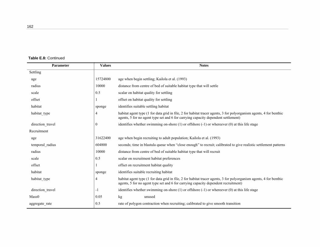
162
Table E.8: Continued
Parameter Values Notes
Settling
age 15724800 age when begin settling; Kailola et al. (1993)
radius 10000 distance from centre of bed of suitable habitat type that will settle
scale 0.5 scalar on habitat quality for settling
offset 1 offset on habitat quality for settling
habitat sponge identifies suitable settling habitat
habitat_type 4 habitat agent type (1 for data grid in file, 2 for habitat tracer agents, 3 for polyorganism agents, 4 for benthic agents, 5 for no agent type set and 6 for carrying capacity dependent settlement)
direction_travel 0 identifies whether swimming on-shore (1) or offshore (-1) or whereever (0) at this life stage
Recruitment
age 31622400 age when begin recruiting to adult population; Kailola et al. (1993)
temporal_radius 604800 seconds; time in blastula queue when “close enough” to recruit; calibrated to give realistic settlement patterns
radius 10000 distance from centre of bed of suitable habitat type that will recruit
scale 0.5 scalar on recruitment habitat preferences
offset 1 offset on recruitment habitat quality
habitat sponge identifies suitable recruiting habitat
habitat_type 4 habitat agent type (1 for data grid in file, 2 for habitat tracer agents, 3 for polyorganism agents, 4 for benthic agents, 5 for no agent type set and 6 for carrying capacity dependent recruitment)
direction_travel -1 identifies whether swimming on-shore (1) or offshore (-1) or whereever (0) at this life stage
Mass0 0.05 kg unused
aggregate_rate 0.5 rate of polygon contraction when recruiting; calibrated to give smooth transition
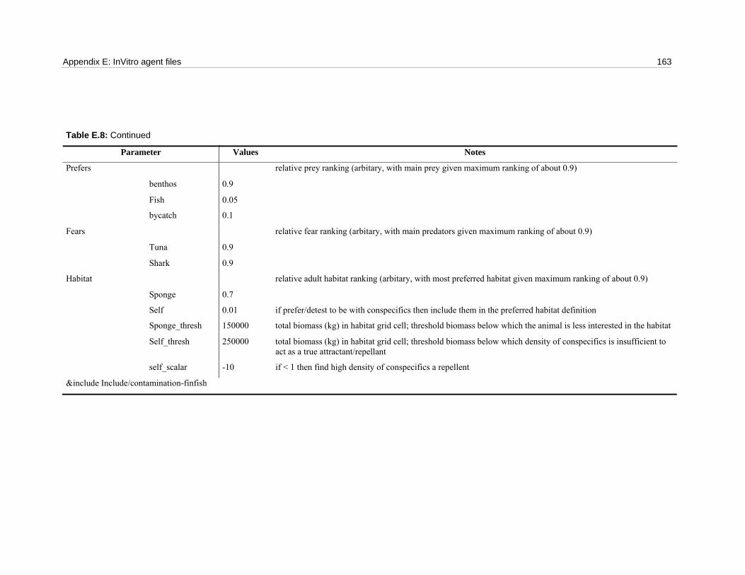
Appendix E: InVitro agent files 163
Table E.8: Continued
Parameter Values Notes
Prefers relative prey ranking (arbitary, with main prey given maximum ranking of about 0.9)
benthos 0.9
Fish 0.05
bycatch 0.1
Fears relative fear ranking (arbitary, with main predators given maximum ranking of about 0.9)
Tuna 0.9
Shark 0.9
Habitat relative adult habitat ranking (arbitary, with most preferred habitat given maximum ranking of about 0.9)
Sponge 0.7
Self 0.01 if prefer/detest to be with conspecifics then include them in the preferred habitat definition
Sponge_thresh 150000 total biomass (kg) in habitat grid cell; threshold biomass below which the animal is less interested in the habitat
Self_thresh 250000 total biomass (kg) in habitat grid cell; threshold biomass below which density of conspecifics is insufficient to act as a true attractant/repellant
self_scalar -10 if < 1 then find high density of conspecifics a repellent
&include Include/contamination-finfish

164
Table E.9: mangroves file - parameters taken from literature or tuned to reflect understanding of system.
Parameter Values Notes
Awareness_type 1 0 for fine scale awareness, 1 for large scale program control parameter – dictating resolution of adviser agent interrogation (see Gray et al. (2006))
tick_length 604800 seconds Typical time step length
bored_tick 1728000 seconds Maximum standard time step length
alarmed_tick 1200 seconds Standard time step length if in active state
really_verbose_vectors 1 put titles in monitor file
RecruitmentOption
default 0
altrecruit1 1
altrecruit2 1
flag indicating recruitment model used (dictates contribution of external source of larvae and the influence of sediment and depth on recruitment success – 0 for based on depth and sediment quality, 1 for based on depth and proportional to are of NWS colonised, 2 for proportion of suitable habitat on NWS, 3 for recruitment based on suitable habitat plus sediment quality and constant supply of external recruits, 4 for recruitment based on proportional habitat cover on the NWS plus sediment quality and constant supply of external recruits , and 5 for recruitment based on suitable habitat colonised plus proportional cover plus sediment quality and constant supply of external recruits)
RecruitmentScalar 100 used to scale recruitment weightings; calibrated
RecruitmentCoefficient 1 steepness of curvature of recruitment curve; calibrated
ClearingDamageRate 0.1 rate of general damage to gridcell due to coastal development clearing; based on Semeniuk (1994), Semeniuk and Semeniuk (1995, 1997)
AcidGrowthReduction 0.05 reduction in growth rate due to acid sulphate leaching
Small
AverageMass 20 kg / square metre based on Robertson and Alongi (1992)
AverageHeight 0.5 metres based on Robertson and Alongi (1992), McGuinness (1997) and Paling (1996)
RecruitRate 0.01 recruitment rate; based on Robertson and Alongi (1992), McGuinness (1997) and Paling (1996)
SpreadRate 0.01 horizontal growth rate per year; estimated - simple least squares estimation
DepthCoefficient 1 depth related recruitment parameter
SedimentCoefficient 1 sediment related recruitment parameter (set to 1.0 as no effect)
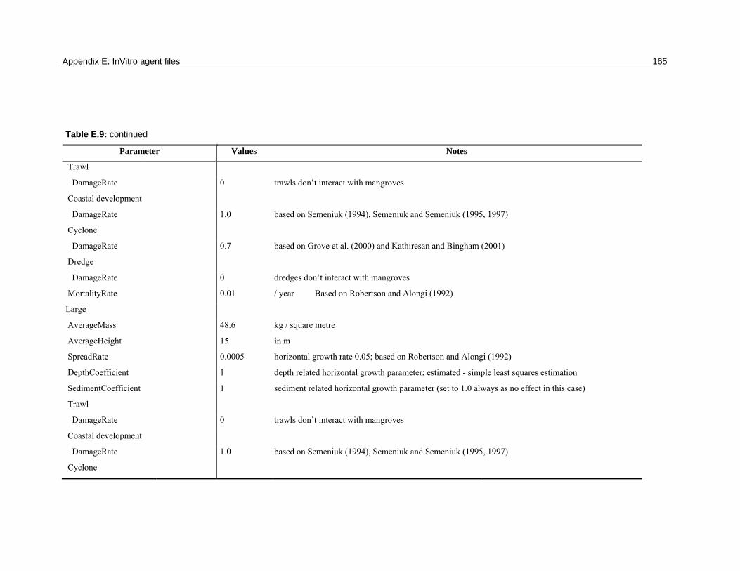
Appendix E: InVitro agent files 165
Table E.9: continued
Parameter Values Notes
Trawl
DamageRate 0 trawls don’t interact with mangroves
Coastal development
DamageRate 1.0 based on Semeniuk (1994), Semeniuk and Semeniuk (1995, 1997)
Cyclone
DamageRate 0.7 based on Grove et al. (2000) and Kathiresan and Bingham (2001)
Dredge
DamageRate 0 dredges don’t interact with mangroves
MortalityRate 0.01 / year Based on Robertson and Alongi (1992)
Large
AverageMass 48.6 kg / square metre
AverageHeight 15 in m
SpreadRate 0.0005 horizontal growth rate 0.05; based on Robertson and Alongi (1992)
DepthCoefficient 1 depth related horizontal growth parameter; estimated - simple least squares estimation
SedimentCoefficient 1 sediment related horizontal growth parameter (set to 1.0 always as no effect in this case)
Trawl
DamageRate 0 trawls don’t interact with mangroves
Coastal development
DamageRate 1.0 based on Semeniuk (1994), Semeniuk and Semeniuk (1995, 1997)
Cyclone
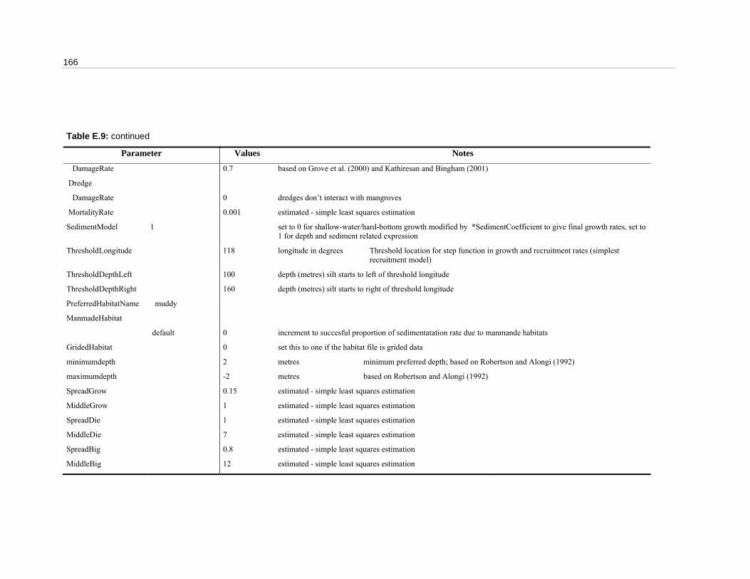
166
Table E.9: continued
Parameter Values Notes
DamageRate 0.7 based on Grove et al. (2000) and Kathiresan and Bingham (2001)
Dredge
DamageRate 0 dredges don’t interact with mangroves
MortalityRate 0.001 estimated - simple least squares estimation
SedimentModel 1 set to 0 for shallow-water/hard-bottom growth modified by *SedimentCoefficient to give final growth rates, set to 1 for depth and sediment related expression
ThresholdLongitude 118 longitude in degrees Threshold location for step function in growth and recruitment rates (simplest recruitment model)
ThresholdDepthLeft 100 depth (metres) silt starts to left of threshold longitude
ThresholdDepthRight 160 depth (metres) silt starts to right of threshold longitude
PreferredHabitatName muddy
ManmadeHabitat
default 0 increment to succesful proportion of sedimentatation rate due to manmande habitats
GridedHabitat 0 set this to one if the habitat file is grided data
minimumdepth 2 metres minimum preferred depth; based on Robertson and Alongi (1992)
maximumdepth -2 metres based on Robertson and Alongi (1992)
SpreadGrow 0.15 estimated - simple least squares estimation
MiddleGrow 1 estimated - simple least squares estimation
SpreadDie 1 estimated - simple least squares estimation
MiddleDie 7 estimated - simple least squares estimation
SpreadBig 0.8 estimated - simple least squares estimation
MiddleBig 12 estimated - simple least squares estimation
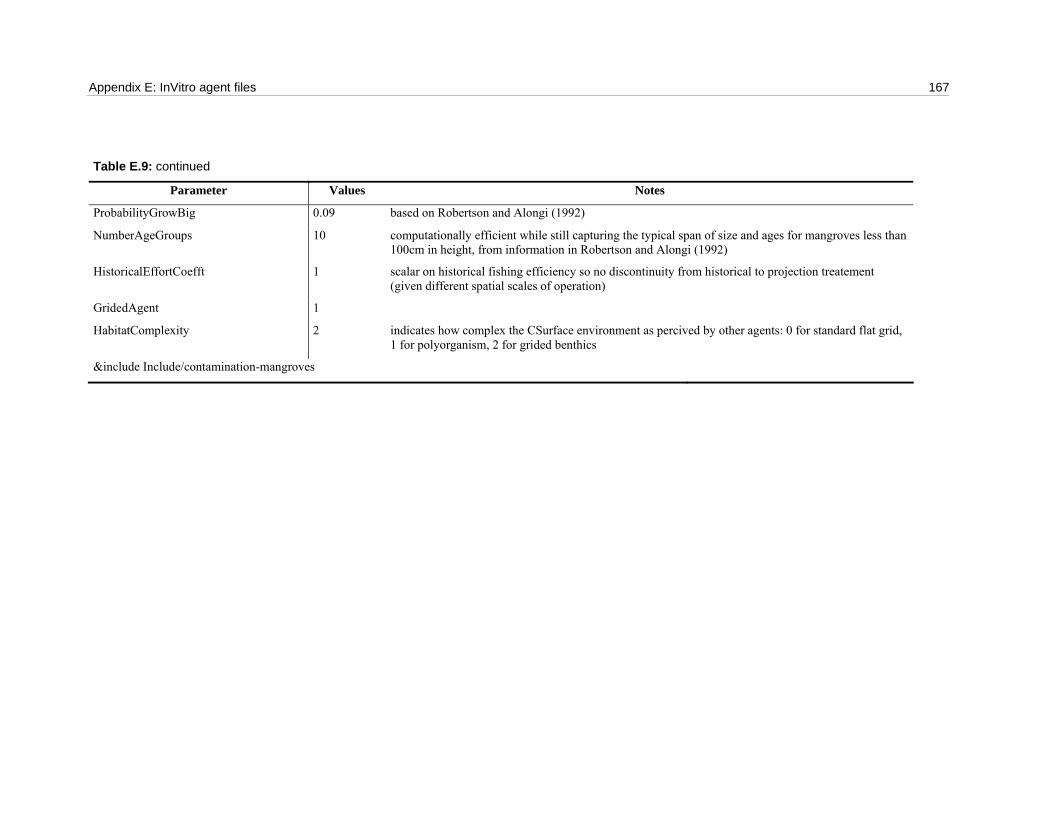
Appendix E: InVitro agent files 167
Table E.9: continued
Parameter Values Notes
ProbabilityGrowBig 0.09 based on Robertson and Alongi (1992)
NumberAgeGroups 10 computationally efficient while still capturing the typical span of size and ages for mangroves less than 100cm in height, from information in Robertson and Alongi (1992)
HistoricalEffortCoefft 1 scalar on historical fishing efficiency so no discontinuity from historical to projection treatement (given different spatial scales of operation)
GridedAgent 1
HabitatComplexity 2 indicates how complex the CSurface environment as percived by other agents: 0 for standard flat grid, 1 for polyorganism, 2 for grided benthics
&include Include/contamination-mangroves

168
Table E.10: nemipterid (nemip) file.
Parameter Values Notes
restricted_area pilbara-closed zones fisheries targeting this species must avoid
control_area pilbara-zones zones fisheries targeting this species must be aware of
Carrying_capacity estimated from Bulman (2006) and gradient parameter search
default 1.50E+07 in kg
Standard 30000000 in kg
Maximum_Age 8 years FISHBASE (2005) and expert opinion (P. Stephenson pers. comm.)
t_zero 1 years Age of maturity (used in mortality calculations); FISHBASE (2005) and expert opinion (P. Stephenson pers. comm.)
Rate_Mortality 0.25 / year FISHBASE (2005) and expert opinion (P. Stephenson pers. comm.)
Catastrophic_Mortality 0 / event mortality rate during catastrophic storm event
Speed 0.7 metres / second cruising speed from FISHBASE (2005)
SpeedScale 0.00009 scale cruising speed by this when dealing to populations; Wall and Przeworski (2000)
MaxSpeed 1.8 metres / second from FISHBASE (2005)
SearchRadiusExponent 2 governs how far afield we assume organisms can detect conditions (estimated on velocity)
Directional_variability 0.5 degree to which they remain moving in a single facing (direction); calibrated
Speed_variability 0.07 stochastic variability in wandering speed; calculated by comparing crusing and maximum speeds in FISHBASE (2005)
Traverse_Time 0.8 months Time taken to cross the entire NWS if swimming directly; calculated from swimming speed, weighted by degree of aggregation (of agent – so populations took longer than fish)
Length_t 0.3 coefficient in length-weight relationship (using length = pow(mass,ln(Length_t)/ln(Mass_t))))
Mass_t 0.4 coefficient in length-weight relationship (using length = pow(mass,ln(Length_t)/ln(Mass_t))))
Width_a 0.04 dimensions of organism; directly measured
Gape/Width 0.15 ratio of gape to width (estimated from direct measurements)
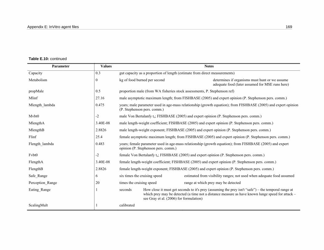
Appendix E: InVitro agent files 169
Table E.10: continued
Parameter Values Notes
Capacity 0.3 gut capacity as a proportion of length (estimate from direct measurements)
Metabolism 0 kg of food burned per second determines if organisms must hunt or we assume adequate food (later assumed for MSE runs here)
propMale 0.5 proportion male (from WA fisheries stock assessments, P. Stephenson ref)
Mlinf 27.16 male asymptotic maximum length; from FISHBASE (2005) and expert opinion (P. Stephenson pers. comm.)
Mlength_lambda 0.475 years; male parameter used in age-mass relationship (growth equation); from FISHBASE (2005) and expert opinion (P. Stephenson pers. comm.)
Mvbt0 -2 male Von Bertalanfy to; FISHBASE (2005) and expert opinion (P. Stephenson pers. comm.)
MlengthA 3.40E-08 male length-weight coefficient; FISHBASE (2005) and expert opinion (P. Stephenson pers. comm.)
MlengthB 2.8826 male length-weight exponent; FISHBASE (2005) and expert opinion (P. Stephenson pers. comm.)
Flinf 25.4 female asymptotic maximum length; from FISHBASE (2005) and expert opinion (P. Stephenson pers. comm.)
Flength_lambda 0.483 years; female parameter used in age-mass relationship (growth equation); from FISHBASE (2005) and expert opinion (P. Stephenson pers. comm.)
Fvbt0 -2 female Von Bertalanfy to; FISHBASE (2005) and expert opinion (P. Stephenson pers. comm.)
FlengthA 3.40E-08 female length-weight coefficient; FISHBASE (2005) and expert opinion (P. Stephenson pers. comm.)
FlengthB 2.8826 female length-weight exponent; FISHBASE (2005) and expert opinion (P. Stephenson pers. comm.)
Safe_Range 6 six times the cruising speed estimated from visibility ranges; not used when adequate food assumed
Perception_Range 20 times the cruising speed range at which prey may be detected
Eating_Range 1 seconds How close it must get seconds to it's prey (assuming the prey isn't “safe”) – the temporal range at which prey may be detected (a time not a distance measure as have known lunge speed for attack – see Gray et al. (2006) for formulation)
ScalingMult 1 calibrated
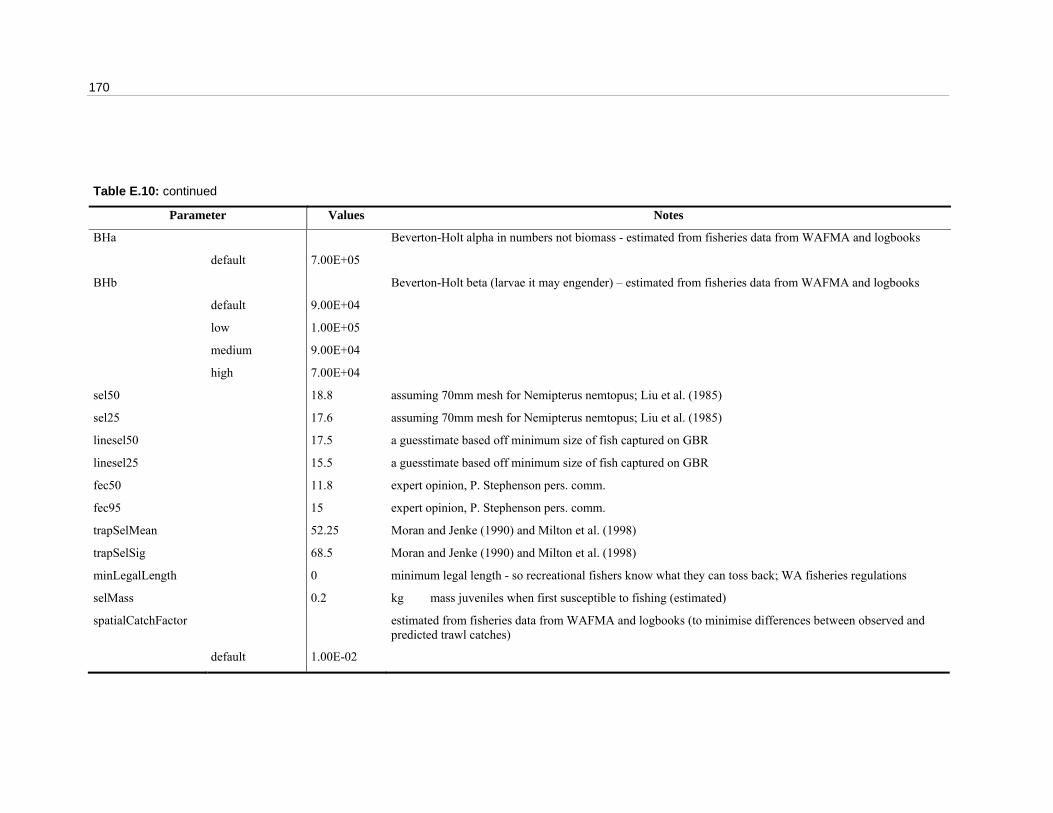
170
Table E.10: continued
Parameter Values Notes
BHa Beverton-Holt alpha in numbers not biomass - estimated from fisheries data from WAFMA and logbooks
default 7.00E+05
BHb Beverton-Holt beta (larvae it may engender) – estimated from fisheries data from WAFMA and logbooks
default 9.00E+04
low 1.00E+05
medium 9.00E+04
high 7.00E+04
sel50 18.8 assuming 70mm mesh for Nemipterus nemtopus; Liu et al. (1985)
sel25 17.6 assuming 70mm mesh for Nemipterus nemtopus; Liu et al. (1985)
linesel50 17.5 a guesstimate based off minimum size of fish captured on GBR
linesel25 15.5 a guesstimate based off minimum size of fish captured on GBR
fec50 11.8 expert opinion, P. Stephenson pers. comm.
fec95 15 expert opinion, P. Stephenson pers. comm.
trapSelMean 52.25 Moran and Jenke (1990) and Milton et al. (1998)
trapSelSig 68.5 Moran and Jenke (1990) and Milton et al. (1998)
minLegalLength 0 minimum legal length - so recreational fishers know what they can toss back; WA fisheries regulations
selMass 0.2 kg mass juveniles when first susceptible to fishing (estimated)
spatialCatchFactor estimated from fisheries data from WAFMA and logbooks (to minimise differences between observed and predicted trawl catches)
default 1.00E-02
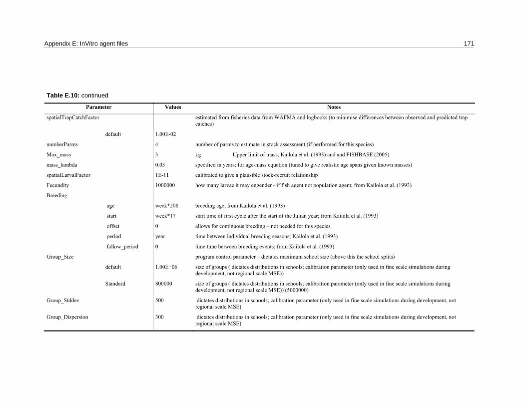
Appendix E: InVitro agent files 171
Table E.10: continued
Parameter Values Notes
spatialTrapCatchFactor estimated from fisheries data from WAFMA and logbooks (to minimise differences between observed and predicted trap catches)
default 1.00E-02
numberParms 4 number of parms to estimate in stock assessment (if performed for this species)
Max_mass 3 kg Upper limit of mass; Kailola et al. (1993) and and FISHBASE (2005)
mass_lambda 0.03 specified in years; for age-mass equation (tuned to give realistic age spans given known masses)
spatialLarvalFactor 1E-11 calibrated to give a plausible stock-recruit relationship
Fecundity 1000000 how many larvae it may engender - if fish agent not population agent; from Kailola et al. (1993)
Breeding
age week*208 breeding age; from Kailola et al. (1993)
start week*17 start time of first cycle after the start of the Julian year; from Kailola et al. (1993)
offset 0 allows for continuous breeding – not needed for this species
period year time between individual breeding seasons; Kailola et al. (1993)
fallow_period 0 time time between breeding events; from Kailola et al. (1993)
Group_Size program control parameter – dictates maximum school size (above this the school splits)
default 1.00E+06 size of groups ( dictates distributions in schools; calibration parameter (only used in fine scale simulations during development, not regional scale MSE))
Standard 800000 size of groups ( dictates distributions in schools; calibration parameter (only used in fine scale simulations during development, not regional scale MSE)) (5000000)
Group_Stddev 500 dictates distributions in schools; calibration parameter (only used in fine scale simulations during development, not regional scale MSE)
Group_Dispersion 300 dictates distributions in schools; calibration parameter (only used in fine scale simulations during development, not regional scale MSE)

172
Table E.10: continued
Parameter Values Notes
Group_Terminal 300 group size below which school disperses when schools drop below this they are culled (if they can not merge first)
Excited_Tick 604800 seconds Standard time step length if in active state
Alarmed_Tick 604800 seconds Standard time step length if in active state
Bored_Tick 7862400 seconds Maximum standard time step length
Tick_Length 7862400 seconds Typical time step length
Minimum_Depth -1 metres minimum preferred depth; Kailola et al. (1993)
Best_Depth -60 metres median preferred depth; Kailola et al. (1993)
Maximum_Depth -180 metres maximum preferred depth; Kailola et al. (1993)
Minimum_Sea_Depth -15 metres minimum depth typically used in marine waters (used to constrain locations in scenarios)
Maximum_Sea_Depth -6000 metres maximum depth typically reached in marine waters (often used to constrain the populations to specific locations for fine scale simulations)
CarryingCapacityAlpha 0.003 mass (kg) of fish supported per kg/m2 of habitat; calculated from Bulman (2006)
CarryingCapacityBeta 300 min square metres required to support a kg of fish; calculated from Bulman (2006)
Masslarva 1 for population this is mass of individual larva in kg
radius 25000 metres school extent
trawl_efficiency 0.1 efficiency of trawlers against species on juvenile stages (expert opinion; P. Stephenson pers. comm.)
assess_environment 1 flag to show whether species seeks favourable environments
Awareness_type 1 0 for fine scale awareness, 1 for large scale program control parameter – dictating resolution of adviser agent interrogation (see Gray et al. (2006))
ScalingBestSeaDepth 0.0001 weighting for influence of preferred depth in guiding habitat selection
Larva juvenile parameters
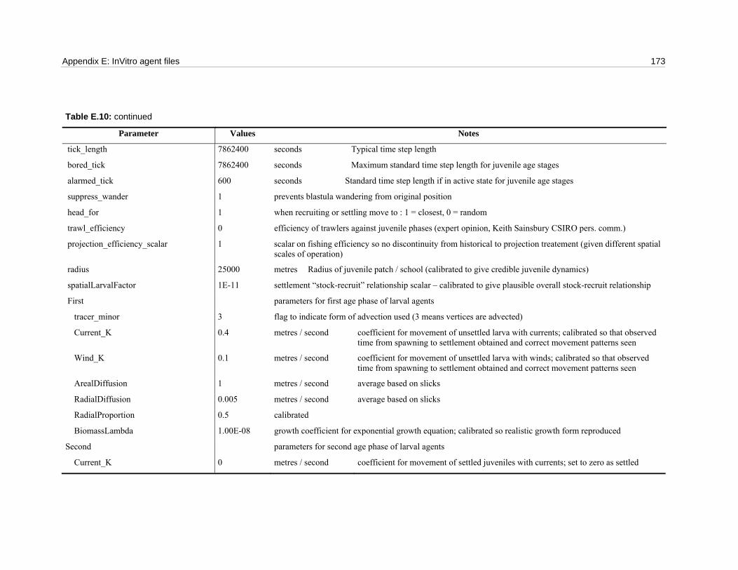
Appendix E: InVitro agent files 173
Table E.10: continued
Parameter Values Notes
tick_length 7862400 seconds Typical time step length
bored_tick 7862400 seconds Maximum standard time step length for juvenile age stages
alarmed_tick 600 seconds Standard time step length if in active state for juvenile age stages
suppress_wander 1 prevents blastula wandering from original position
head_for 1 when recruiting or settling move to : 1 = closest, 0 = random
trawl_efficiency 0 efficiency of trawlers against juvenile phases (expert opinion, Keith Sainsbury CSIRO pers. comm.)
projection_efficiency_scalar 1 scalar on fishing efficiency so no discontinuity from historical to projection treatement (given different spatial scales of operation)
radius 25000 metres Radius of juvenile patch / school (calibrated to give credible juvenile dynamics)
spatialLarvalFactor 1E-11 settlement “stock-recruit” relationship scalar – calibrated to give plausible overall stock-recruit relationship
First parameters for first age phase of larval agents
tracer_minor 3 flag to indicate form of advection used (3 means vertices are advected)
Current_K 0.4 metres / second coefficient for movement of unsettled larva with currents; calibrated so that observed time from spawning to settlement obtained and correct movement patterns seen
Wind_K 0.1 metres / second coefficient for movement of unsettled larva with winds; calibrated so that observed time from spawning to settlement obtained and correct movement patterns seen
ArealDiffusion 1 metres / second average based on slicks
RadialDiffusion 0.005 metres / second average based on slicks
RadialProportion 0.5 calibrated
BiomassLambda 1.00E-08 growth coefficient for exponential growth equation; calibrated so realistic growth form reproduced
Second parameters for second age phase of larval agents
Current_K 0 metres / second coefficient for movement of settled juveniles with currents; set to zero as settled
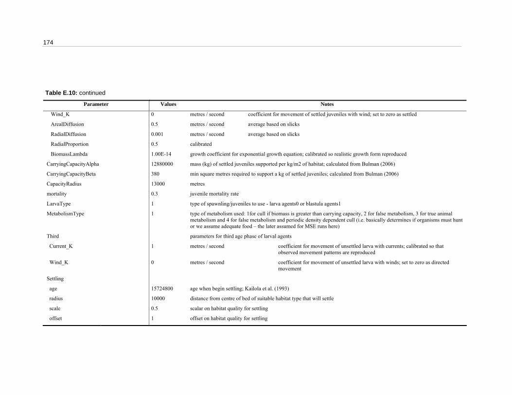
174
Table E.10: continued
Parameter Values Notes
Wind_K 0 metres / second coefficient for movement of settled juveniles with wind; set to zero as settled
ArealDiffusion 0.5 metres / second average based on slicks
RadialDiffusion 0.001 metres / second average based on slicks
RadialProportion 0.5 calibrated
BiomassLambda 1.00E-14 growth coefficient for exponential growth equation; calibrated so realistic growth form reproduced
CarryingCapacityAlpha 12880000 mass (kg) of settled juveniles supported per kg/m2 of habitat; calculated from Bulman (2006)
CarryingCapacityBeta 380 min square metres required to support a kg of settled juveniles; calculated from Bulman (2006)
CapacityRadius 13000 metres
mortality 0.3 juvenile mortality rate
LarvaType 1 type of spawnling/juveniles to use - larva agents0 or blastula agents1
MetabolismType 1 type of metabolism used: 1for cull if biomass is greater than carrying capacity, 2 for false metabolism, 3 for true animal metabolism and 4 for false metabolism and periodic density dependent cull (i.e. basically determines if organisms must hunt or we assume adequate food – the later assumed for MSE runs here)
Third parameters for third age phase of larval agents
Current_K 1 metres / second coefficient for movement of unsettled larva with currents; calibrated so that observed movement patterns are reproduced
Wind_K 0 metres / second coefficient for movement of unsettled larva with winds; set to zero as directed movement
Settling
age 15724800 age when begin settling; Kailola et al. (1993)
radius 10000 distance from centre of bed of suitable habitat type that will settle
scale 0.5 scalar on habitat quality for settling
offset 1 offset on habitat quality for settling

Appendix E: InVitro agent files 175
Table E.10: continued
Parameter Values Notes
habitat sponge identifies suitable settling habitat
habitat_type 4 habitat agent type (1 for data grid in file, 2 for habitat tracer agents, 3 for polyorganism agents, 4 for benthic agents, 5 for no agent type set and 6 for carrying capacity dependent settlement)
direction_travel -1 identifies whether swimming on-shore (1) or offshore (-1) or �herever (0) at this life stage
Recruitment
age 31622400 age when begin recruiting to adult population; Kailola et al. (1993)
temporal_radius 604800 seconds; time in blastula queue when “close enough” to recruit; calibrated to give realistic settlement patterns
radius 200000 distance from centre of bed of suitable habitat type that will recruit
scale 0.5 scalar on recruitment habitat preferences
offset 1 offset on recruitment habitat quality
habitat sponge identifies suitable recruiting habitat
habitat_type 5 habitat agent type (1 for data grid in file, 2 for habitat tracer agents, 3 for polyorganism agents, 4 for benthic agents, 5 for no agent type set and 6 for carrying capacity dependent recruitment)
direction_travel -1 identifies whether swimming on-shore (1) or offshore (-1) or �herever (0) at this life stage
Mass0 0.05 kg unused
aggregate_rate 1 rate of polygon contraction when recruiting; calibrated to give smooth transition
Prefers relative prey ranking (arbitary, with main prey given maximum ranking of about 0.9)
benthos 0.9
Fish 0.05
bycatch 0.1
Fears relative fear ranking (arbitary, with main predators given maximum ranking of about 0.9)

176
Table E.10: continued
Parameter Values Notes
Tuna 0.9
Shark 0.9
Habitat relative adult habitat ranking (arbitary, with most preferred habitat given maximum ranking of about 0.9)
Sponge 0.1
seagrass 0.1
Self 0.01 If prefer/detest to be with conspecifics then include them in the preferred habitat definition
Sponge_thresh 150000 total biomass (kg) in habitat grid cell; threshold biomass below which the animal is less interested in the habitat
seagrass_thresh 80000 total biomass (kg) in habitat grid cell; threshold biomass below which the animal is less interested in the habitat
Self_thresh 750000 total biomass (kg) in habitat grid cell; threshold biomass below which density of conspecifics is insufficient to act as a true attractant/repellant
Self_scalar -10 If < 1 then find high density of conspecifics a repellent
&include Include/contamination-finfish

Appendix E: InVitro agent files 177
Table E.11: oysterlease file – specifies parameters for commercial oyster production.
Parameter Values Notes
monitor_environments Bitterns, Calcium, Sulphate, Zinc, Cadmium, Copper, Lead, Oil, PetroleumHydrocarbons, Tin
selects environmental contaminants to monitor
Suppress_Wander 1 used to prevent oysters wandering
Suppress_Breeding 1 used to prevent oyster leases breeding; renders all members of the species sterile and disinterested
Excited_Tick 604800 seconds Standard time step length if in active state
Alarmed_Tick 604800 seconds Standard time step length if in active state
Bored_Tick 7862400 seconds Maximum standard time step length
Tick_Length 7862400 seconds Typical time step length
&include Include/contamination-oysters

178
Table E.12: saurid (saur) file.
Parameter Values Notes
restricted_area pilbara-closed zones fisheries targeting this species must avoid
control_area pilbara-zones zones fisheries targeting this species must be aware of
Carrying_capacity estimated from Bulman (2006) and gradient parameter search
default 1.50E+07 in kg
Standard 30000000 in kg
Maximum_Age 40 years FISHBASE (2005) and expert opinion (P. Stephenson pers. comm.)
t_zero 1 years Age of maturity (used in mortality calculations); FISHBASE (2005) and expert opinion (P. Stephenson pers. comm.)
Rate_Mortality 0.1 / year FISHBASE (2005) and expert opinion (P. Stephenson pers. comm.)
Catastrophic_Mortality 0 / event mortality rate during catastrophic storm event
Speed 0.7 metres / second cruising speed from FISHBASE (2005)
SpeedScale 0.0001 scale cruising speed by this when dealing to populations; Wall and Przeworski (2000)
MaxSpeed 1.8 metres / second from FISHBASE (2005)
SearchRadiusExponent 2 governs how far afield we assume organisms can detect conditions (estimated on velocity)
Directional_variability 0.5 degree to which they remain moving in a single facing (direction); calibrated
Speed_variability 0.07 stochastic variability in wandering speed; calculated by comparing crusing and maximum speeds in FISHBASE (2005)
Traverse_Time 10 months Time taken to cross the entire NWS if swimming directly; calculated from swimming speed, weighted by degree of aggregation (of agent – so populations took longer than fish)
Length_t 0.4 coefficient in length-weight relationship (using length = pow(mass,ln(Length_t)/ln(Mass_t))))
Mass_t 1.2 coefficient in length-weight relationship (using length = pow(mass,ln(Length_t)/ln(Mass_t))))
Width_a 0.08 dimensions of organism; directly measured
Gape/Width 0.15 ratio of gape to width (estimated from direct measurements)
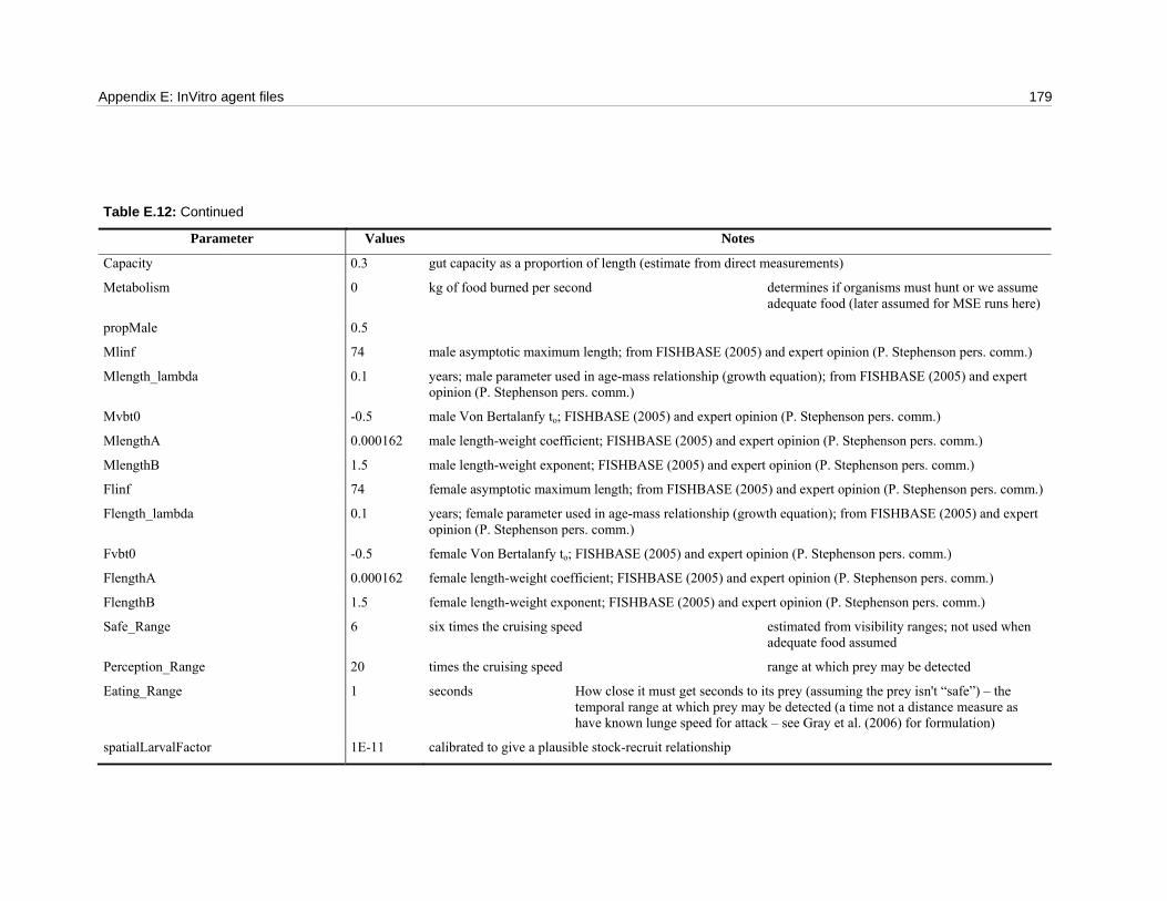
Appendix E: InVitro agent files 179
Table E.12: Continued
Parameter Values Notes
Capacity 0.3 gut capacity as a proportion of length (estimate from direct measurements)
Metabolism 0 kg of food burned per second determines if organisms must hunt or we assume adequate food (later assumed for MSE runs here)
propMale 0.5
Mlinf 74 male asymptotic maximum length; from FISHBASE (2005) and expert opinion (P. Stephenson pers. comm.)
Mlength_lambda 0.1 years; male parameter used in age-mass relationship (growth equation); from FISHBASE (2005) and expert opinion (P. Stephenson pers. comm.)
Mvbt0 -0.5 male Von Bertalanfy to; FISHBASE (2005) and expert opinion (P. Stephenson pers. comm.)
MlengthA 0.000162 male length-weight coefficient; FISHBASE (2005) and expert opinion (P. Stephenson pers. comm.)
MlengthB 1.5 male length-weight exponent; FISHBASE (2005) and expert opinion (P. Stephenson pers. comm.)
Flinf 74 female asymptotic maximum length; from FISHBASE (2005) and expert opinion (P. Stephenson pers. comm.)
Flength_lambda 0.1 years; female parameter used in age-mass relationship (growth equation); from FISHBASE (2005) and expert opinion (P. Stephenson pers. comm.)
Fvbt0 -0.5 female Von Bertalanfy to; FISHBASE (2005) and expert opinion (P. Stephenson pers. comm.)
FlengthA 0.000162 female length-weight coefficient; FISHBASE (2005) and expert opinion (P. Stephenson pers. comm.)
FlengthB 1.5 female length-weight exponent; FISHBASE (2005) and expert opinion (P. Stephenson pers. comm.)
Safe_Range 6 six times the cruising speed estimated from visibility ranges; not used when adequate food assumed
Perception_Range 20 times the cruising speed range at which prey may be detected
Eating_Range 1 seconds How close it must get seconds to its prey (assuming the prey isn't “safe”) – the temporal range at which prey may be detected (a time not a distance measure as have known lunge speed for attack – see Gray et al. (2006) for formulation)
spatialLarvalFactor 1E-11 calibrated to give a plausible stock-recruit relationship

180
Table E.12: Continued
Parameter Values Notes
ScalingMult 0.9 calibrated
BHa Beverton-Holt alpha in numbers not biomass – estimated from fisheries data from WAFMA and logbooks
default 3.00E+04
BHb Beverton-Holt beta (larvae it may engender) – estimated from fisheries data from WAFMA and logbooks
default 5.00E+04
low 6.00E+04
medium 5.00E+04
high 1.00E+04
sel50 21.01 assuming 55mm mesh size for Saurida undosquamis; Liu et al. (1985)
sel25 15.6 assuming 55mm mesh size for Saurida undosquamis; Liu et al. (1985)
linesel50 75.5 set so that not impossible to catch them, but rare (as more a trawl than a line fish)
linesel25 68.5 set so that not impossible to catch them, but rare (as more a trawl than a line fish)
fec50 21 expert opinion, P. Stephenson pers. comm.
Fec95 24 expert opinion, P. Stephenson pers. comm.
trapSelMean 52.25 Moran and Jenke (1990) and Milton et al.(1998)
trapSelSig 68.5 Moran and Jenke (1990) and Milton et al. (1998)
minLegalLength 0 minimum legal length – so recreational fishers know what they can toss back; WA fisheries regulations
selMass 0.2 kg mass juveniles when first susceptible to fishing (estimated)
spatialCatchFactor estimated from fisheries data from WAFMA and logbooks (to minimise differences between observed and predicted trawl catches)

Appendix E: InVitro agent files 181
Table E.12: Continued
Parameter Values Notes
default 1.00E-02
spatialTrapCatchFactor estimated from fisheries data from WAFMA and logbooks (to minimise differences between observed and predicted trap catches)
default 1.00E-02
numberParms 3 number of parms to estimate in stock assessment (if performed for this species)
Max_mass 3 kg Upper limit of mass; Kailola et al. (1993) and and FISHBASE (2005)
mass_lambda 0.03 specified in years; for age-mass equation (tuned to give realistic age spans given known masses)
Fecundity 1000000 how many larvae it may engender - if fish agent not population agent; from Kailola et al. (1993)
Breeding
age week*208 breeding age; from Kailola et al. (1993)
start week*30 start time of first cycle after the start of the Julian year; from Kailola et al. (1993)
offset 0 allows for continuous breeding – not needed for this species
period year time between individual breeding seasons; Kailola et al. (1993)
fallow_period 0 time time between breeding events; from Kailola et al. (1993)
Group_Size program control parameter – dictates maximum school size (above this the school splits)
default 5.00E+05 size of groups ( dictates distributions in schools; calibration parameter (only used in fine scale simulations during development, not regional scale MSE))
Standard 1000000 size of groups ( dictates distributions in schools; calibration parameter (only used in fine scale simulations during development, not regional scale MSE))
Group_Stddev 500 dictates distributions in schools; calibration parameter (only used in fine scale simulations during development, not regional scale MSE)
Group_Dispersion 300 dictates distributions in schools; calibration parameter (only used in fine scale simulations during development, not regional scale MSE)

182
Table E.12: Continued
Parameter Values Notes
Group_Terminal 300 group size below which school disperses when schools drop below this they are culled (if they can not merge first)
Excited_Tick 604800 seconds Standard time step length if in active state
Alarmed_Tick 604800 seconds Standard time step length if in active state
Bored_Tick 7862400 seconds Maximum standard time step length
Tick_Length 7862400 seconds Typical time step length
Minimum_Depth -1 metres minimum preferred depth; Kailola et al. (1993)
Best_Depth -90 metres median preferred depth; Kailola et al. (1993)
Maximum_Depth -200 metres maximum preferred depth; Kailola et al. (1993)
Minimum_Sea_Depth -15 metres minimum depth typically used in marine waters (used to constrain locations in scenarios)
Maximum_Sea_Depth -6000 metres maximum depth typically reached in marine waters (often used to constrain the populations to specific locations for fine scale simulations)
Masslarva 1 for population this is mass of individual larva in kg, for fish it is a scalar for recruits (defaul value 1.0)
radius 40000 metres school extent
trawl_efficiency 0.1 efficiency of trawlers against species on juvenile stages (expert opinion; P. Stephenson pers. comm.)
assess_environment 1 flag to show whether species seeks favourable environments
Awareness_type 1 0 for fine scale awareness, 1 for large scale program control parameter – dictating resolution of adviser agent interrogation (see Gray et al. (2006))
ScalingBestSeaDepth 0.0001 weighting for influence of preferred depth in guiding habitat selection
Larva juvenile parameters
tick_length 7862400 seconds Typical time step length for juvenile age stages
bored_tick 7862400 seconds Maximum standard time step length for for juvenile age stages
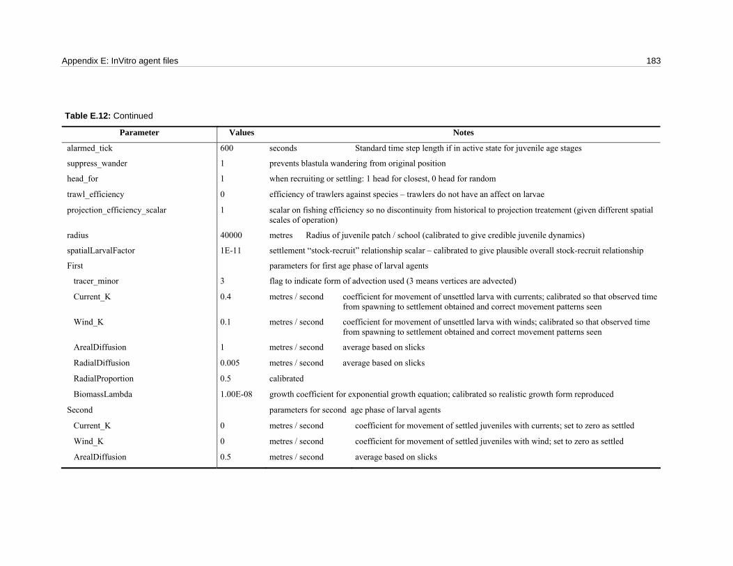
Appendix E: InVitro agent files 183
Table E.12: Continued
Parameter Values Notes
alarmed_tick 600 seconds Standard time step length if in active state for juvenile age stages
suppress_wander 1 prevents blastula wandering from original position
head_for 1 when recruiting or settling: 1 head for closest, 0 head for random
trawl_efficiency 0 efficiency of trawlers against species – trawlers do not have an affect on larvae
projection_efficiency_scalar 1 scalar on fishing efficiency so no discontinuity from historical to projection treatement (given different spatial scales of operation)
radius 40000 metres Radius of juvenile patch / school (calibrated to give credible juvenile dynamics)
spatialLarvalFactor 1E-11 settlement “stock-recruit” relationship scalar – calibrated to give plausible overall stock-recruit relationship
First parameters for first age phase of larval agents
tracer_minor 3 flag to indicate form of advection used (3 means vertices are advected)
Current_K 0.4 metres / second coefficient for movement of unsettled larva with currents; calibrated so that observed time from spawning to settlement obtained and correct movement patterns seen
Wind_K 0.1 metres / second coefficient for movement of unsettled larva with winds; calibrated so that observed time from spawning to settlement obtained and correct movement patterns seen
ArealDiffusion 1 metres / second average based on slicks
RadialDiffusion 0.005 metres / second average based on slicks
RadialProportion 0.5 calibrated
BiomassLambda 1.00E-08 growth coefficient for exponential growth equation; calibrated so realistic growth form reproduced
Second parameters for second age phase of larval agents
Current_K 0 metres / second coefficient for movement of settled juveniles with currents; set to zero as settled
Wind_K 0 metres / second coefficient for movement of settled juveniles with wind; set to zero as settled
ArealDiffusion 0.5 metres / second average based on slicks
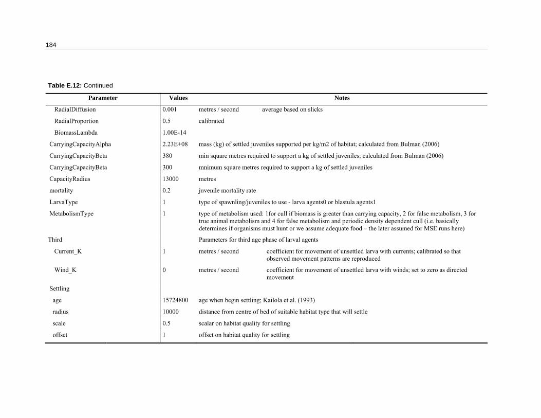
184
Table E.12: Continued
Parameter Values Notes
RadialDiffusion 0.001 metres / second average based on slicks
RadialProportion 0.5 calibrated
BiomassLambda 1.00E-14
CarryingCapacityAlpha 2.23E+08 mass (kg) of settled juveniles supported per kg/m2 of habitat; calculated from Bulman (2006)
CarryingCapacityBeta 380 min square metres required to support a kg of settled juveniles; calculated from Bulman (2006)
CarryingCapacityBeta 300 mnimum square metres required to support a kg of settled juveniles
CapacityRadius 13000 metres
mortality 0.2 juvenile mortality rate
LarvaType 1 type of spawnling/juveniles to use - larva agents0 or blastula agents1
MetabolismType 1 type of metabolism used: 1for cull if biomass is greater than carrying capacity, 2 for false metabolism, 3 for true animal metabolism and 4 for false metabolism and periodic density dependent cull (i.e. basically determines if organisms must hunt or we assume adequate food – the later assumed for MSE runs here)
Third Parameters for third age phase of larval agents
Current_K 1 metres / second coefficient for movement of unsettled larva with currents; calibrated so that observed movement patterns are reproduced
Wind_K 0 metres / second coefficient for movement of unsettled larva with winds; set to zero as directed movement
Settling
age 15724800 age when begin settling; Kailola et al. (1993)
radius 10000 distance from centre of bed of suitable habitat type that will settle
scale 0.5 scalar on habitat quality for settling
offset 1 offset on habitat quality for settling

Appendix E: InVitro agent files 185
Table E.12: Continued
Parameter Values Notes
habitat sponge identifies suitable settling habitat
habitat_type 5 habitat agent type (1 for data grid in file, 2 for habitat tracer agents, 3 for polyorganism agents, 4 for benthic agents, 5 for no agent type set and 6 for carrying capacity dependent settlement)
direction_travel 0 identifies whether swimming on-shore (1) or offshore (-1) or �herever (0) at this life stage
Recruitment
age 31622400 age when begin recruiting to adult population; Kailola et al. (1993)
temporal_radius 604800 seconds; time in blastula queue when “close enough” to recruit; calibrated to give realistic settlement patterns
radius 200000 distance from centre of bed of suitable habitat type that will recruit
scale 0.5 scalar on recruitment habitat preferences
offset 1 offset on recruitment habitat quality
habitat sponge identifies suitable recruiting habitat
habitat_type 5 habitat agent type (1 for data grid in file, 2 for habitat tracer agents, 3 for polyorganism agents, 4 for benthic agents, 5 for no agent type set and 6 for carrying capacity dependent recruitment)
direction_travel -1 identifies whether swimming on-shore (1) or offshore (-1) or �herever (0) at this life stage
Mass0 0.05 kg UNUSED
aggregate_rate 1 rate of polygon contraction when recruiting; calibrated to give smooth transition
Prefers relative prey ranking (arbitary, with main prey given maximum ranking of about 0.9)
benthos 0.9
fish 0.05
bycatch 0.1
Fears relative fear ranking (arbitary, with main predators given maximum ranking of about 0.9)
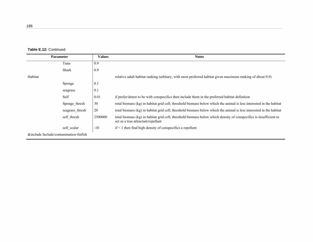
186
Table E.12: Continued
Parameter Values Notes
Tuna 0.9
Shark 0.9
Habitat relative adult habitat ranking (arbitary, with most preferred habitat given maximum ranking of about 0.9)
Sponge 0.1
seagrass 0.1
Self 0.01 if prefer/detest to be with conspecifics then include them in the preferred habitat definition
Sponge_thresh 30 total biomass (kg) in habitat grid cell; threshold biomass below which the animal is less interested in the habitat
seagrass_thresh 20 total biomass (kg) in habitat grid cell; threshold biomass below which the animal is less interested in the habitat
self_thresh 2500000 total biomass (kg) in habitat grid cell; threshold biomass below which density of conspecifics is insufficient to act as a true attractant/repellant
self_scalar -10 if < 1 then find high density of conspecifics a repellent
&include Include/contamination-finfish

Appendix E: InVitro agent files 187
Table E.13: seagrass file - parameters taken from literature or tuned to reflect understanding of system.
Parameter Values Notes
tick_length 604800 seconds Typical time step length
bored_tick 1728000 seconds Maximum standard time step length
alarmed_tick 1200 seconds Standard time step length if in active state
ClearingDamageRate 0 rate of damage to gridcell due to coastal development clearing
AcidGrowthReduction 0 reduction in growth rate due to acid sulphate leaching
Small
AverageMass 0.2 kg / square metre based on Bulman (2006)
AverageHeight 0.2 metres Clayton and King (1990)
RecruitRate 0.3 recruitment rate; Campbell (2003)
SpreadRate 0.5 horizontal growth rate ; based on Cambridge et al. (2002) and Campbell (2003)
DepthCoefficient 0.1 depth related recruitment parameter; estimated
SedimentCoefficient 1 sediment related recruitment parameter; estimated
Trawl
DamageRate 0.8 vulnerability to trawling; based on Hall (1999) and Meyer et al. (1999)
Cyclone
DamageRate 0.4 vulnerability to cyclones; based on Preen et al. (1995)
Dredge
DamageRate 1 vulnerability to dredging; based on Cheshire and Miller (1996)
MortalityRate 0.2 / year based on van Tussenbroek (2002) and Biber et al., (2004)
Large
AverageMass 1 kg / square metre Based on Bulman (2006)
AverageHeight 0.5 in m Creed et al. (1998), Alberg (1992)
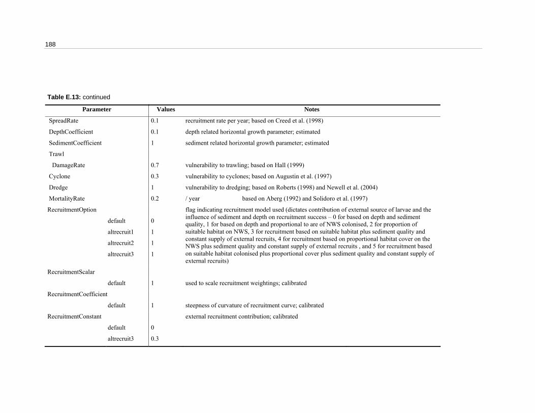
188
Table E.13: continued
Parameter Values Notes
SpreadRate 0.1 recruitment rate per year; based on Creed et al. (1998)
DepthCoefficient 0.1 depth related horizontal growth parameter; estimated
SedimentCoefficient 1 sediment related horizontal growth parameter; estimated
Trawl
DamageRate 0.7 vulnerability to trawling; based on Hall (1999)
Cyclone 0.3 vulnerability to cyclones; based on Augustin et al. (1997)
Dredge 1 vulnerability to dredging; based on Roberts (1998) and Newell et al. (2004)
MortalityRate 0.2 / year based on Aberg (1992) and Solidoro et al. (1997)
RecruitmentOption
default 0
altrecruit1 1
altrecruit2 1
altrecruit3 1
flag indicating recruitment model used (dictates contribution of external source of larvae and the influence of sediment and depth on recruitment success – 0 for based on depth and sediment quality, 1 for based on depth and proportional to are of NWS colonised, 2 for proportion of suitable habitat on NWS, 3 for recruitment based on suitable habitat plus sediment quality and constant supply of external recruits, 4 for recruitment based on proportional habitat cover on the NWS plus sediment quality and constant supply of external recruits , and 5 for recruitment based on suitable habitat colonised plus proportional cover plus sediment quality and constant supply of external recruits)
RecruitmentScalar
default 1 used to scale recruitment weightings; calibrated
RecruitmentCoefficient
default 1 steepness of curvature of recruitment curve; calibrated
RecruitmentConstant external recruitment contribution; calibrated
default 0
altrecruit3 0.3
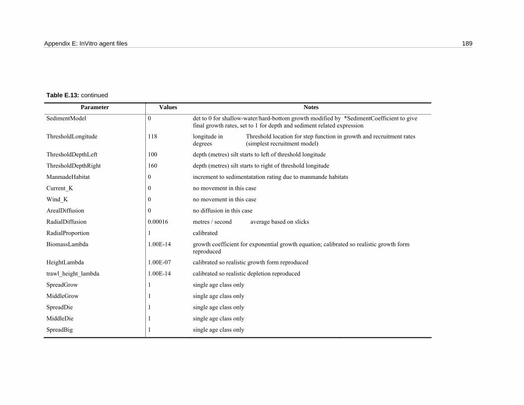
Appendix E: InVitro agent files 189
Table E.13: continued
Parameter Values Notes
SedimentModel 0 det to 0 for shallow-water/hard-bottom growth modified by *SedimentCoefficient to give final growth rates, set to 1 for depth and sediment related expression
ThresholdLongitude 118 longitude in degrees
Threshold location for step function in growth and recruitment rates (simplest recruitment model)
ThresholdDepthLeft 100 depth (metres) silt starts to left of threshold longitude
ThresholdDepthRight 160 depth (metres) silt starts to right of threshold longitude
ManmadeHabitat 0 increment to sedimentatation rating due to manmande habitats
Current_K 0 no movement in this case
Wind_K 0 no movement in this case
ArealDiffusion 0 no diffusion in this case
RadialDiffusion 0.00016 metres / second average based on slicks
RadialProportion 1 calibrated
BiomassLambda 1.00E-14 growth coefficient for exponential growth equation; calibrated so realistic growth form reproduced
HeightLambda 1.00E-07 calibrated so realistic growth form reproduced
trawl_height_lambda 1.00E-14 calibrated so realistic depletion reproduced
SpreadGrow 1 single age class only
MiddleGrow 1 single age class only
SpreadDie 1 single age class only
MiddleDie 1 single age class only
SpreadBig 1 single age class only

190
Table E.13: continued
Parameter Values Notes
MiddleBig 1 single age class only
ProbabilityGrowBig 0 single age class only so no transition necessary
NumberAgeGroups 2 single age class only for seagrass and macroalgae
HistoricalEffortCoefft 0.0001 scalar on historical fishing efficiency so no discontinuity from historical to projection treatement (given different spatial scales of operation)
GridedAgent 1
HabitatComplexity 2 indicates how complex the CSurface environment as percived by other agents: 0standard flat grid, 1polyorganism, 2grided benthics
PreferredHabitatName sandy
SuitableHabitatFile sed381.xy.pt
minimum_depth -1.0 metres minimum preferred depth; Clayton and King (1990)
maximum_depth -50.0 metres maximum preferred depth; Clayton and King (1990)
&include Include/contamination-seagrass

Appendix E: InVitro agent files 191
Table E.14: small lutjanids (slut) file.
Parameter Values Notes
restricted_area pilbara-closed zones fisheries targeting this species must avoid
control_area pilbara-zones zones fisheries targeting this species must be aware of
Carrying_capacity estimated from Bulman (2006) and gradient parameter search
Default 1.50E+07 in kg
Standard 15000000 in kg
Maximum_Age 12 years FISHBASE (2005) and expert opinion (P. Stephenson pers. comm.)
t_zero 1 years Age of maturity (used in mortality calculations); FISHBASE (2005) and expert opinion (P. Stephenson pers. comm.)
Rate_Mortality 0.25 / year FISHBASE (2005) and expert opinion (P. Stephenson pers. comm.)
Catastrophic_Mortality 0 / event mortality rate during catastrophic storm event
Speed 0.7 metres / second cruising speed from FISHBASE (2005)
SpeedScale 0.00009 scale cruising speed by this when dealing to populations; Wall and Przeworski (2000)
MaxSpeed 1.8 metres / second from FISHBASE (2005)
SearchRadiusExponent 2 governs how far afield we assume organisms can detect conditions (estimated on velocity)
Directional_variability 0.5 degree to which they remain moving in a single facing (direction); calibrated
Speed_variability 0.07 stochastic variability in wandering speed; calculated by comparing crusing and maximum speeds in FISHBASE (2005)
Traverse_Time 10 months Time taken to cross the entire NWS if swimming directly; calculated from swimming speed, weighted by degree of aggregation (of agent – so populations took longer than fish)
Length_t 0.55 coefficient in length-weight relationship (using length = pow(mass,ln(Length_t)/ln(Mass_t))))
Mass_t 1.7 coefficient in length-weight relationship (using length = pow(mass,ln(Length_t)/ln(Mass_t))))
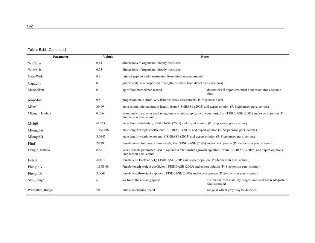
192
Table E.14: Continued
Parameter Values Notes
Width_a 0.14 dimensions of organism; directly measured
Width_b 0.25 dimensions of organism; directly measured
Gape/Width 0.9 ratio of gape to width (estimated from direct measurements)
Capacity 0.3 gut capacity as a proportion of length (estimate from direct measurements)
Metabolism 0 kg of food burned per second determines if organisms must hunt or assume adequate food
propMale 0.5 proportion male (from WA fisheries stock assessments, P. Stephenson ref)
Mlinf 30.19 male asymptotic maximum length; from FISHBASE (2005) and expert opinion (P. Stephenson pers. comm.)
Mlength_lambda 0.706 years; male parameter used in age-mass relationship (growth equation); from FISHBASE (2005) and expert opinion (P. Stephenson pers. comm.)
Mvbt0 -0.333 male Von Bertalanfy to; FISHBASE (2005) and expert opinion (P. Stephenson pers. comm.)
MlengthA 1.19E-08 male length-weight coefficient; FISHBASE (2005) and expert opinion (P. Stephenson pers. comm.)
MlengthB 3.0645 male length-weight exponent; FISHBASE (2005) and expert opinion (P. Stephenson pers. comm.)
Flinf 29.29 female asymptotic maximum length; from FISHBASE (2005) and expert opinion (P. Stephenson pers. comm.)
Flength_lambda 0.661 years; female parameter used in age-mass relationship (growth equation); from FISHBASE (2005) and expert opinion (P. Stephenson pers. comm.)
Fvbt0 -0.801 female Von Bertalanfy to; FISHBASE (2005) and expert opinion (P. Stephenson pers. comm.)
FlengthA 1.19E-08 female length-weight coefficient; FISHBASE (2005) and expert opinion (P. Stephenson pers. comm.)
FlengthB 3.0645 female length-weight exponent; FISHBASE (2005) and expert opinion (P. Stephenson pers. comm.)
Safe_Range 6 six times the cruising speed Estimated from visibility ranges; not used when adequate food assumed
Perception_Range 20 times the cruising speed range at which prey may be detected

Appendix E: InVitro agent files 193
Table E.14: Continued
Parameter Values Notes
Eating_Range 1 seconds How close it must get seconds to it's prey (assuming the prey isn't “safe”) – the temporal range at which prey may be detected (a time not a distance measure as have known lunge speed for attack – see Gray et al. (2006) for formulation)
ScalingMult 0.9 calibrated
BHa Beverton-Holt alpha in numbers not biomass - estimated from fisheries data from WAFMA and logbooks
Default 1.00E+05
Low 3.00E+05
Medium 1.00E+05
High 9.00E+05
BHb Beverton-Holt beta (larvae it may engender) – estimated from fisheries data from WAFMA and logbooks
Default 1.00E+04
Low 9.00E+04
Medium 1.00E+04
High 3.00E+05
sel50 28.5 (~3.5years); expert opinion, P. Stephenson pers. comm.
sel25 24.21 (~3.5years); expert opinion, P. Stephenson pers. comm.
linesel50 15.5 a guesstimate based off minimum size of fish captured on GBR
linesel25 12.5 a guesstimate based off minimum size of fish captured on GBR
fec50 18.5 expert opinion, P. Stephenson pers. comm.
fec95 22 expert opinion, P. Stephenson pers. comm.
trapSelMean 52.25 Moran and Jenke (1990) and Milton et al. (1998)
trapSelSig 68.5 Moran and Jenke (1990) and Milton et al. (1998)

194
Table E.14: Continued
Parameter Values Notes
minLegalLength 30 minimum legal length - so recreational fishers know what they can toss back; WA fisheries regulations
selMass 0.2 kg mass juveniles when first susceptible to fishing (estimated)
spatialCatchFactor
estimated from fisheries data from WAFMA and logbooks (to minimise differences between observed and predicted trawl catches)
default 1.00E-02
spatialTrapCatchFactor estimated from fisheries data from WAFMA and logbooks (to minimise differences between observed and predicted trap catches)
default 1.00E-02
numberParms 4 number of parms to estimate in stock assessment (if performed for this species)
Max_mass 7.9 kg Upper limit of mass; Kailola et al. (1993) and and FISHBASE (2005)
mass_lambda 0.03 specified in years; for age-mass equation (tuned to give realistic age spans given known masses)
spatialLarvalFactor 1E-11 calibrated to give a plausible stock-recruit relationship
Fecundity 1000000 how many larvae it may engender - if fish agent not population agent; from Kailola et al. (1993)
Breeding
age week*208 breeding age; from Kailola et al. (1993)
start week*17 start time of first cycle after the start of the Julian year; from Kailola et al. (1993)
offset 0 allows for continuous breeding – not needed for this species
period year time between individual breeding seasons; Kailola et al. (1993)
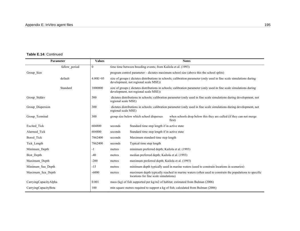
Appendix E: InVitro agent files 195
Table E.14: Continued
Parameter Values Notes
fallow_period 0 time time between breeding events; from Kailola et al. (1993)
Group_Size program control parameter – dictates maximum school size (above this the school splits)
default 4.00E+05 size of groups ( dictates distributions in schools; calibration parameter (only used in fine scale simulations during development, not regional scale MSE))
Standard 1000000 size of groups ( dictates distributions in schools; calibration parameter (only used in fine scale simulations during development, not regional scale MSE))
Group_Stddev 500 dictates distributions in schools; calibration parameter (only used in fine scale simulations during development, not regional scale MSE)
Group_Dispersion 300 dictates distributions in schools; calibration parameter (only used in fine scale simulations during development, not regional scale MSE)
Group_Terminal 300 group size below which school disperses when schools drop below this they are culled (if they can not merge first)
Excited_Tick 604800 seconds Standard time step length if in active state
Alarmed_Tick 604800 seconds Standard time step length if in active state
Bored_Tick 7862400 seconds Maximum standard time step length
Tick_Length 7862400 seconds Typical time step length
Minimum_Depth -1 metres minimum preferred depth; Kailola et al. (1993)
Best_Depth -40 metres median preferred depth; Kailola et al. (1993)
Maximum_Depth -200 metres maximum preferred depth; Kailola et al. (1993)
Minimum_Sea_Depth -15 metres minimum depth typically used in marine waters (used to constrain locations in scenarios)
Maximum_Sea_Depth -6000 metres maximum depth typically reached in marine waters (often used to constrain the populations to specific locations for fine scale simulations)
CarryingCapacityAlpha 0.001 mass (kg) of fish supported per kg/m2 of habitat; estimated from Bulman (2006)
CarryingCapacityBeta 100 min square metres required to support a kg of fish; calculated from Bulman (2006)

196
Table E.14: Continued
Parameter Values Notes
Masslarva 1 for population this is mass of individual juvenile in kg; direct measurement (1.0e-9default)
radius 25000 metres school extent
trawl_efficiency 0.1 efficiency of trawlers against species on juvenile stages (expert opinion; P. Stephenson pers. comm.)
assess_environment 1 flag to show whether species seeks favourable environments
Awareness_type 1 0 for fine scale awareness, 1 for large scale
program control parameter – dictating resolution of adviser agent interrogation (see Gray et al. (2006))
ScalingBestSeaDepth
default 0.0001 weighting for influence of preferred depth in guiding habitat selection
Larva juvenile parameters
tick_length 7862400 seconds Typical time step length for juvenile age phases
bored_tick 7862400 seconds Maximum standard time step length for juvenile age phases
alarmed_tick 600 seconds Standard time step length if in active state for juvenile age stages
suppress_wander 1 prevents blastula wandering from original position
head_for 1 flag setting whether they head for random spot or closest when recruiting or settling: 1=heading for closest, 0=heading for random
trawl_efficiency 0 efficiency of trawlers against juvenile stages (expert opinion, Keith Sainsbury CSIRO pers. comm.)
projection_efficiency_scalar 1 scalar on fishing efficiency so no discontinuity from historical to projection treatement (given different spatial scales of operation)
radius 25000 metres Radius of juvenile patch / school (calibrated to give credible juvenile dynamics)
spatialLarvalFactor 1E-11 settlement “stock-recruit” relationship scalar – calibrated to give plausible overall stock-recruit relationship
First parameters for first age phase of larval agents
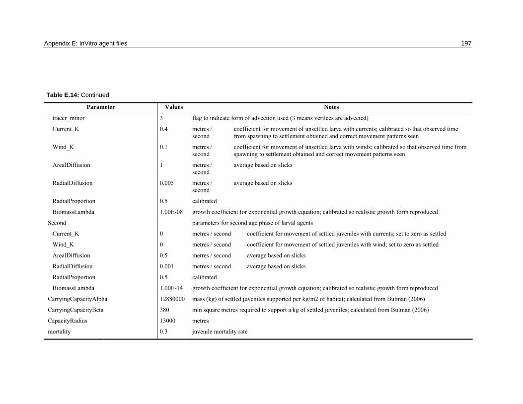
Appendix E: InVitro agent files 197
Table E.14: Continued
Parameter Values Notes
tracer_minor 3 flag to indicate form of advection used (3 means vertices are advected)
Current_K 0.4 metres / second
coefficient for movement of unsettled larva with currents; calibrated so that observed time from spawning to settlement obtained and correct movement patterns seen
Wind_K 0.1 metres / second
coefficient for movement of unsettled larva with winds; calibrated so that observed time from spawning to settlement obtained and correct movement patterns seen
ArealDiffusion 1 metres / second
average based on slicks
RadialDiffusion 0.005 metres / second
average based on slicks
RadialProportion 0.5 calibrated
BiomassLambda 1.00E-08 growth coefficient for exponential growth equation; calibrated so realistic growth form reproduced
Second parameters for second age phase of larval agents
Current_K 0 metres / second coefficient for movement of settled juveniles with currents; set to zero as settled
Wind_K 0 metres / second coefficient for movement of settled juveniles with wind; set to zero as settled
ArealDiffusion 0.5 metres / second average based on slicks
RadialDiffusion 0.001 metres / second average based on slicks
RadialProportion 0.5 calibrated
BiomassLambda 1.00E-14 growth coefficient for exponential growth equation; calibrated so realistic growth form reproduced
CarryingCapacityAlpha 12880000 mass (kg) of settled juveniles supported per kg/m2 of habitat; calculated from Bulman (2006)
CarryingCapacityBeta 380 min square metres required to support a kg of settled juveniles; calculated from Bulman (2006)
CapacityRadius 13000 metres
mortality 0.3 juvenile mortality rate

198
Table E.14: Continued
Parameter Values Notes
LarvaType 1 type of spawnling/juveniles to use - larva agents0 or blastula agents1
MetabolismType 1 type of metabolism used: 1for cull if biomass is greater than carrying capacity, 2 for false metabolism, 3 for true animal metabolism and 4 for false metabolism and periodic density dependent cull (i.e. basically determines if organisms must hunt or we assume adequate food – the later assumed for MSE runs here)
Third Parameters for third age phase of larval agents
Current_K 1 metres / second
coefficient for movement of unsettled larva with currents; calibrated so that observed movement patterns are reproduced
Wind_K 0 metres / second
coefficient for movement of unsettled larva with winds; set to zero as directed movement
Settling
age 15724800 age when begin settling; Kailola et al. (1993)
radius 10000 distance from centre of bed of suitable habitat type that will settle
scale 0.5 scalar on habitat quality for settling
offset 1 offset on habitat quality for settling
habitat sponge identifies suitable settling habitat
habitat_type 4 habitat agent type (1 for data grid in file, 2 for habitat tracer agents, 3 for polyorganism agents, 4 for benthic agents, 5 for no agent type set and 6 for carrying capacity dependent settlement)
direction_travel -1 identifies whether swimming on-shore (1) or offshore (-1) or whereever (0) at this life stage
Recruitment
age 31622400 age when begin recruiting to adult population; Kailola et al. (1993)
temporal_radius 604800 seconds; time in blastula queue when “close enough” to recruit; calibrated to give realistic settlement patterns
radius 200000 distance from centre of bed of suitable habitat type that will recruit

Appendix E: InVitro agent files 199
Table E.14: Continued
Parameter Values Notes
scale 0.5 scalar on recruitment habitat preferences
offset 1 offset on recruitment habitat quality
habitat sponge identifies suitable recruiting habitat
habitat_type 4 habitat agent type (1 for data grid in file, 2 for habitat tracer agents, 3 for polyorganism agents, 4 for benthic agents, 5 for no agent type set and 6 for carrying capacity dependent recruitment)
direction_travel -1 identifies whether swimming on-shore (1) or offshore (-1) or whereever (0) at this life stage
Mass0 0.05 kg unused
aggregate_rate 1 rate of polygon contraction when recruiting; calibrated to give smooth transition
Prefers relative prey ranking (arbitary, with main prey given maximum ranking of about 0.9)
benthos 0.9
fish 0.05
bycatch 0.1
Fears relative fear ranking (arbitary, with main predators given maximum ranking of about 0.9)
Tuna 0.9
Shark 0.9
Habitat relative adult habitat ranking (arbitary, with most preferred habitat given maximum ranking of about 0.9)
Sponge 0.7
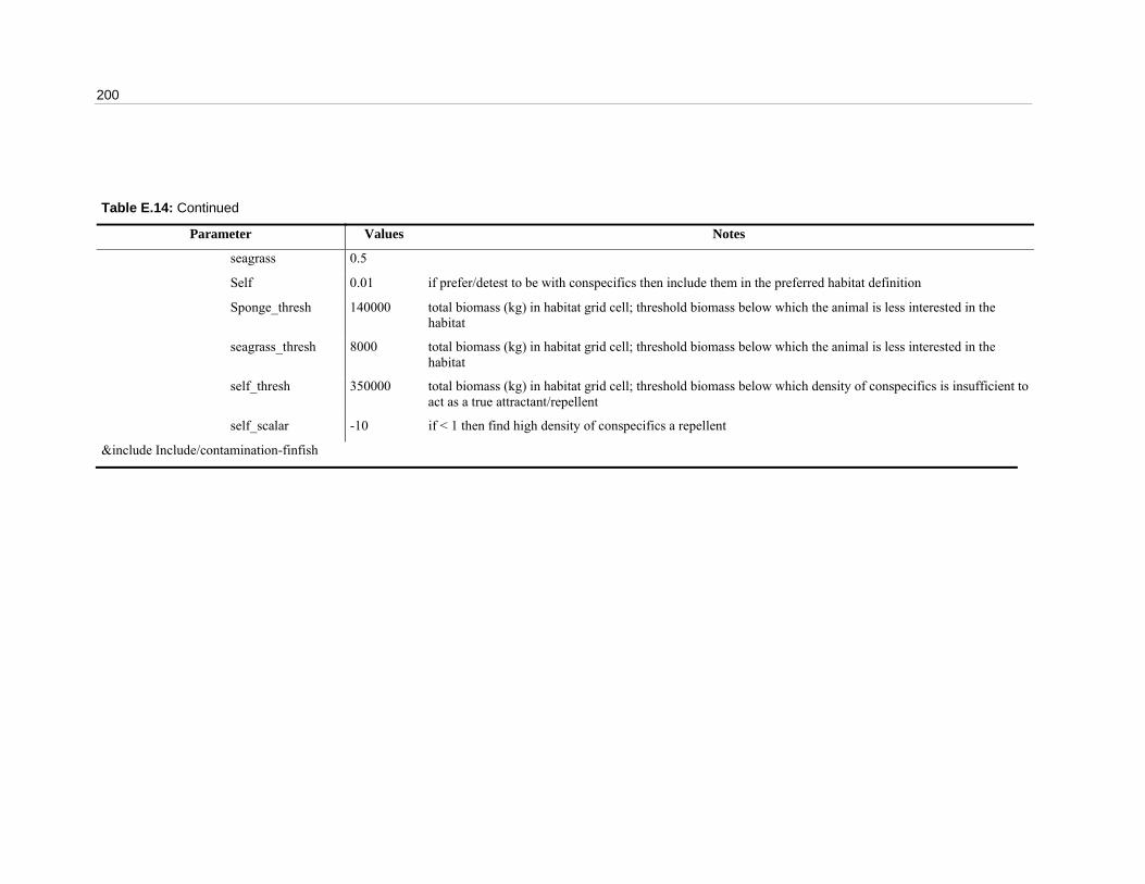
200
Table E.14: Continued
Parameter Values Notes
seagrass 0.5
Self 0.01 if prefer/detest to be with conspecifics then include them in the preferred habitat definition
Sponge_thresh 140000 total biomass (kg) in habitat grid cell; threshold biomass below which the animal is less interested in the habitat
seagrass_thresh 8000 total biomass (kg) in habitat grid cell; threshold biomass below which the animal is less interested in the habitat
self_thresh 350000 total biomass (kg) in habitat grid cell; threshold biomass below which density of conspecifics is insufficient to act as a true attractant/repellent
self_scalar -10 if < 1 then find high density of conspecifics a repellent
&include Include/contamination-finfish

Appendix E: InVitro agent files 201
Table E.15: shark file - parameters taken from literature or tuned to reflect understanding of system.
Parameter Values Notes
may_nest program control parameter - allows for nesting of this agent type within other agents
fish 1
default 1
blastula 0
eggmortality determines pre-larval mortality applied to number of eggs produced
default 1 the ratio of eggs surviving to settlement to the number originally spawned. Calculated by solving for the rate that leads to a stable population level.
cull_period week*4 periodicity of natural mortality (tuned to runtime resolution)
Carrying_capacity 330000 in kg Estimated from Bulman (2006)
Maximum_Age 65 years FISHBASE (2005)
t_zero 1 years Age of maturity (used in mortality calculations);
Rate_Mortality 0.095 / year expert opinion, Fred Pribac pers. comm.
Catastrophic_Mortality 0 / event mortality rate during catastrophic storm event
Speed 0.02 metres / second cruising speed; from FISHBASE (2005)
MaxSpeed 0.05 metres /second from FISHBASE (2005)
SearchRadiusExponent 4 governs how far afield we assume organisms can detect conditions (estimated on velocity)
Directional_variability 0.8 degree to which they remain moving in a single facing (direction); calibrated
Speed_variability 0.07 stochastic variability in wandering speed; calculated by comparing crusing and maximum speeds in FISHBASE (2005)
Traverse_Time 0.1 months Time taken to cross the entire NWS if swimming directly; calculated from swimming speed, weighted by degree of aggregation (of agent – so populations took longer than fish)
Length_t 3 coefficient in length-weight relationship (using length = pow(mass,ln(Length_t)/ln(Mass_t))))
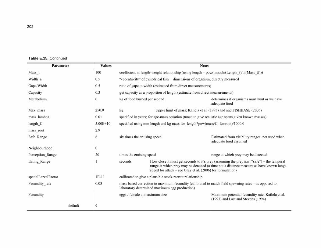
202
Table E.15: Continued
Parameter Values Notes
Mass_t 100 coefficient in length-weight relationship (using length = pow(mass,ln(Length_t)/ln(Mass_t))))
Width_a 0.5 “eccentricity” of cylindrical fish dimensions of organism; directly measured
Gape/Width 0.5 ratio of gape to width (estimated from direct measurements)
Capacity 0.3 gut capacity as a proportion of length (estimate from direct measurements)
Metabolism 0 kg of food burned per second determines if organisms must hunt or we have adequate food
Max_mass 250.0 kg Upper limit of mass; Kailola et al. (1993) and and FISHBASE (2005)
mass_lambda 0.01 specified in years; for age-mass equation (tuned to give realistic age spans given known masses)
length_C 5.00E+10 specified using mm length and kg mass for length*pow(mass/C, 1/mroot)/1000.0
mass_root 2.9
Safe_Range 6 six times the cruising speed Estimated from visibility ranges; not used when adequate food assumed
Neighbourhood 0
Perception_Range 20 times the cruising speed range at which prey may be detected
Eating_Range 1 seconds How close it must get seconds to it's prey (assuming the prey isn't “safe”) – the temporal range at which prey may be detected (a time not a distance measure as have known lunge speed for attack – see Gray et al. (2006) for formulation)
spatialLarvalFactor 1E-11 calibrated to give a plausible stock-recruit relationship
Fecundity_rate 0.03 mass based correction to maximum fecundity (calibrated to match field spawning rates – as opposed to laboratory determined maximum egg production)
Fecundity eggs / female at maximum size Maximum potential fecundity rate; Kailola et al. (1993) and Last and Stevens (1994)
default 9
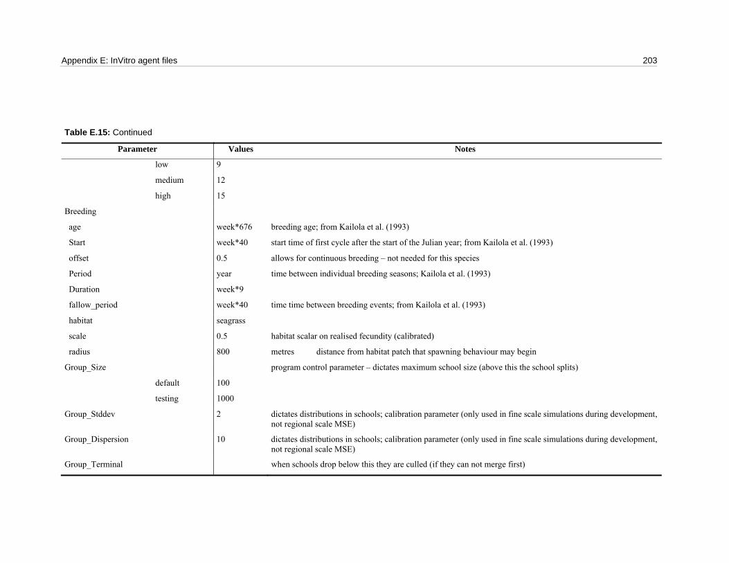
Appendix E: InVitro agent files 203
Table E.15: Continued
Parameter Values Notes
low 9
medium 12
high 15
Breeding
age week*676 breeding age; from Kailola et al. (1993)
Start week*40 start time of first cycle after the start of the Julian year; from Kailola et al. (1993)
offset 0.5 allows for continuous breeding – not needed for this species
Period year time between individual breeding seasons; Kailola et al. (1993)
Duration week*9
fallow_period week*40 time time between breeding events; from Kailola et al. (1993)
habitat seagrass
scale 0.5 habitat scalar on realised fecundity (calibrated)
radius 800 metres distance from habitat patch that spawning behaviour may begin
Group_Size program control parameter – dictates maximum school size (above this the school splits)
default 100
testing 1000
Group_Stddev 2 dictates distributions in schools; calibration parameter (only used in fine scale simulations during development, not regional scale MSE)
Group_Dispersion 10 dictates distributions in schools; calibration parameter (only used in fine scale simulations during development, not regional scale MSE)
Group_Terminal when schools drop below this they are culled (if they can not merge first)
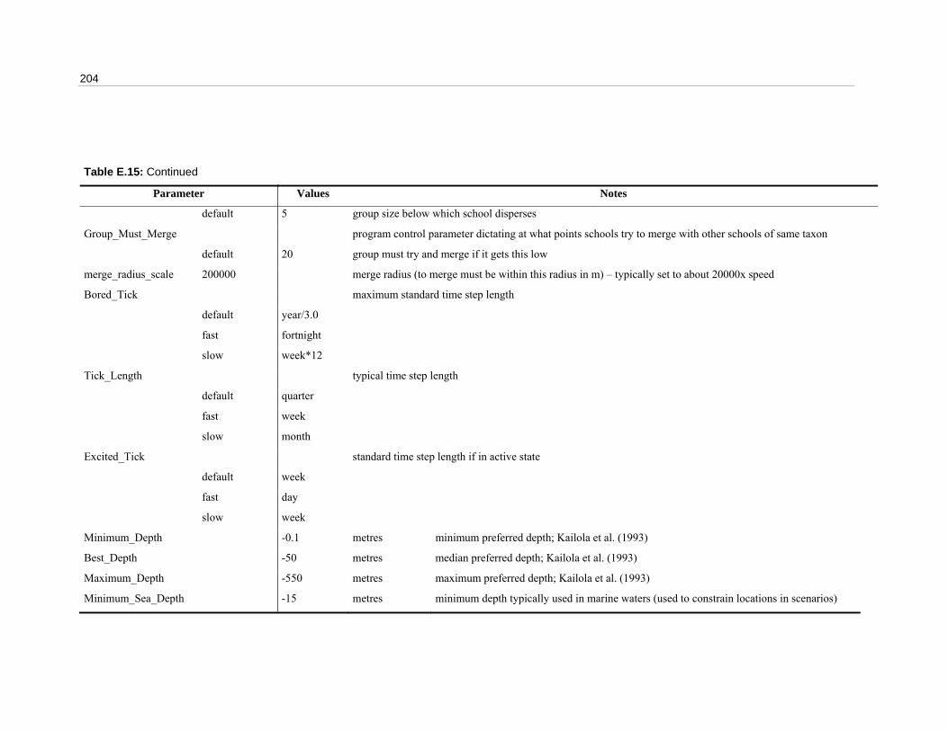
204
Table E.15: Continued
Parameter Values Notes
default 5 group size below which school disperses
Group_Must_Merge program control parameter dictating at what points schools try to merge with other schools of same taxon
default 20 group must try and merge if it gets this low
merge_radius_scale 200000 merge radius (to merge must be within this radius in m) – typically set to about 20000x speed
Bored_Tick maximum standard time step length
default year/3.0
fast fortnight
slow week*12
Tick_Length typical time step length
default quarter
fast week
slow month
Excited_Tick standard time step length if in active state
default week
fast day
slow week
Minimum_Depth -0.1 metres minimum preferred depth; Kailola et al. (1993)
Best_Depth -50 metres median preferred depth; Kailola et al. (1993)
Maximum_Depth -550 metres maximum preferred depth; Kailola et al. (1993)
Minimum_Sea_Depth -15 metres minimum depth typically used in marine waters (used to constrain locations in scenarios)
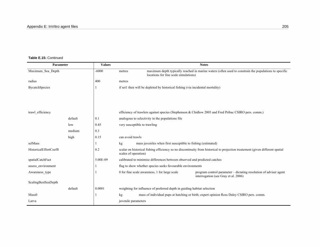
Appendix E: InVitro agent files 205
Table E.15: Continued
Parameter Values Notes
Maximum_Sea_Depth -6000 metres maximum depth typically reached in marine waters (often used to constrain the populations to specific locations for fine scale simulations)
radius 400 metres
BycatchSpecies 1 if set1 then will be depleted by historical fishing (via incidental mortality)
trawl_efficiency
efficiency of trawlers against species (Stephenson & Chidlow 2003 and Fred Pribac CSIRO pers. comm.)
default 0.1 analogous to selectivity in the populations file
low 0.45 very susceptible to trawling
medium 0.3
high 0.15 can avoid trawls
selMass 1 kg mass juveniles when first susceptible to fishing (estimated)
HistoricalEffortCoefft 0.2 scalar on historical fishing efficiency so no discontinuity from historical to projection treatement (given different spatial scales of operation)
spatialCatchFact 5.00E-09 calibrated to minimise differences between observed and predicted catches
assess_environment 1 flag to show whether species seeks favourable environments
Awareness_type 1 0 for fine scale awareness, 1 for large scale program control parameter – dictating resolution of adviser agent interrogation (see Gray et al. 2006)
ScalingBestSeaDepth
default 0.0001 weighting for influence of preferred depth in guiding habitat selection
Mass0 1 kg mass of individual pups at hatching or birth; expert opinion Ross Daley CSIRO pers. comm.
Larva juvenile parameters

206
Table E.15: Continued
Parameter Values Notes
MetabolismType 4 determines if organisms must hunt or we assume adequate food (later assumed for MSE runs here)
tick_length 1200 seconds Typical time step length for juvenile age stages
bored_tick 81400 seconds Maximum standard time step length for juvenile age stages
alarmed_tick 600 seconds Standard time step length if in active state for juvenile age stages
head_for 1 flag setting whether they head for random spot or closest when recruiting or settling: (1 for heading for closest, 0 for heading for random)
trawl_efficiency 0 baby sharks too small to be caught in trawls (as not born yet really but lets skip the “if caught mum” complication for now)
projection_efficiency_scalar 1 scalar on fishing efficiency so no discontinuity from historical to projection treatement (given different spatial scales of operation)
radius 400 metres Radius of juvenile patch / school (calibrated to give credible juvenile dynamics)
spatialLarvalFactor 1E-11 settlement “stock-recruit” relationship scalar – calibrated to give plausible overall stock-recruit relationship
CarryingCapacityAlpha 0.00012 mass (kg) of settled juveniles supported per kg/m2 of habitat; calculated from Bulman (2006)
CarryingCapacityBeta 6000 mnimum square metres required to support a kg of settled juveniles; calculated from Bulman (2006)
CapacityRadius 13000 metres
mortality 0.3 juvenile mortality rate
Settling
age 86400 age when begin settling; Kailola et al. (1993) and Last and Stevens (1994)
radius 10000 distance from centre of bed of suitable habitat type that will settle
scale 0.5 scalar on habitat quality for settling
offset 1 offset on habitat quality for settling
habitat identifies suitable settling habitat
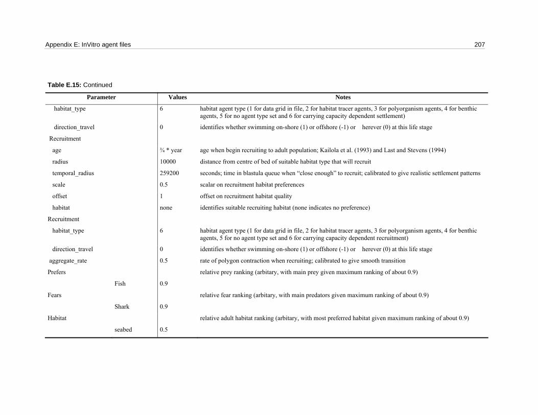
Appendix E: InVitro agent files 207
Table E.15: Continued
Parameter Values Notes
habitat_type 6 habitat agent type (1 for data grid in file, 2 for habitat tracer agents, 3 for polyorganism agents, 4 for benthic agents, 5 for no agent type set and 6 for carrying capacity dependent settlement)
direction_travel 0 identifies whether swimming on-shore (1) or offshore (-1) or �herever (0) at this life stage
Recruitment
age ¾ * year age when begin recruiting to adult population; Kailola et al. (1993) and Last and Stevens (1994)
radius 10000 distance from centre of bed of suitable habitat type that will recruit
temporal_radius 259200 seconds; time in blastula queue when “close enough” to recruit; calibrated to give realistic settlement patterns
scale 0.5 scalar on recruitment habitat preferences
offset 1 offset on recruitment habitat quality
habitat none identifies suitable recruiting habitat (none indicates no preference)
Recruitment
habitat_type 6 habitat agent type (1 for data grid in file, 2 for habitat tracer agents, 3 for polyorganism agents, 4 for benthic agents, 5 for no agent type set and 6 for carrying capacity dependent recruitment)
direction_travel 0 identifies whether swimming on-shore (1) or offshore (-1) or �herever (0) at this life stage
aggregate_rate 0.5 rate of polygon contraction when recruiting; calibrated to give smooth transition
Prefers relative prey ranking (arbitary, with main prey given maximum ranking of about 0.9)
Fish 0.9
Fears relative fear ranking (arbitary, with main predators given maximum ranking of about 0.9)
Shark 0.9
Habitat relative adult habitat ranking (arbitary, with most preferred habitat given maximum ranking of about 0.9)
seabed 0.5
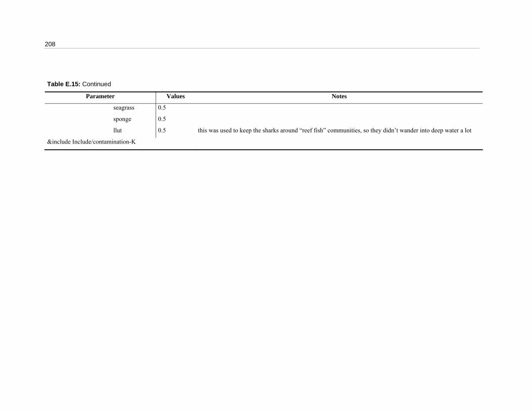
208
Table E.15: Continued
Parameter Values Notes
seagrass 0.5
sponge 0.5
llut 0.5 this was used to keep the sharks around “reef fish” communities, so they didn’t wander into deep water a lot
&include Include/contamination-K
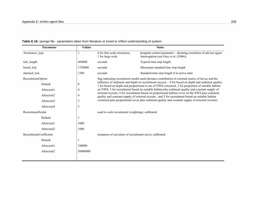
Appendix E: InVitro agent files 209
Table E.16: sponge file - parameters taken from literature or tuned to reflect understanding of system.
Parameter Values Notes
Awareness_type 1 0 for fine scale awareness, 1 for large scale
program control parameter – dictating resolution of adviser agent interrogation (see Gray et al. (2006))
tick_length 604800 seconds Typical time step length
bored_tick 1728000 seconds Maximum standard time step length
alarmed_tick 1200 seconds Standard time step length if in active state
RecruitmentOption
Default 0
Altrecruit1 4
Altrecruit2 4
Altrecruit3 5
Altrecruit4 5
flag indicating recruitment model used (dictates contribution of external source of larvae and the influence of sediment and depth on recruitment success – 0 for based on depth and sediment quality, 1 for based on depth and proportional to are of NWS colonised, 2 for proportion of suitable habitat on NWS, 3 for recruitment based on suitable habitat plus sediment quality and constant supply of external recruits, 4 for recruitment based on proportional habitat cover on the NWS plus sediment quality and constant supply of external recruits , and 5 for recruitment based on suitable habitat colonised plus proportional cover plus sediment quality and constant supply of external recruits)
RecruitmentScalar used to scale recruitment weightings; calibrated
Default 1
Altrecruit1 1000
Altrecruit2 1000
RecruitmentCoefficient steepness of curvature of recruitment curve; calibrated
Default 1
Altrecruit1 100000
Altrecruit2 50000000
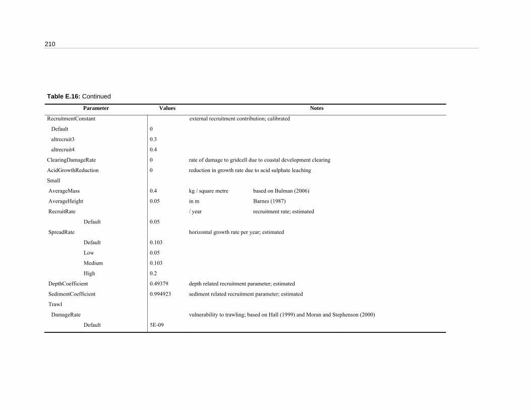
210
Table E.16: Continued
Parameter Values Notes
RecruitmentConstant external recruitment contribution; calibrated
Default 0
altrecruit3 0.3
altrecruit4 0.4
ClearingDamageRate 0 rate of damage to gridcell due to coastal development clearing
AcidGrowthReduction 0 reduction in growth rate due to acid sulphate leaching
Small
AverageMass 0.4 kg / square metre based on Bulman (2006)
AverageHeight 0.05 in m Barnes (1987)
RecruitRate / year recruitment rate; estimated
Default 0.05
SpreadRate horizontal growth rate per year; estimated
Default 0.103
Low 0.05
Medium 0.103
High 0.2
DepthCoefficient 0.49379 depth related recruitment parameter; estimated
SedimentCoefficient 0.994923 sediment related recruitment parameter; estimated
Trawl
DamageRate vulnerability to trawling; based on Hall (1999) and Moran and Stephenson (2000)
Default 5E-09
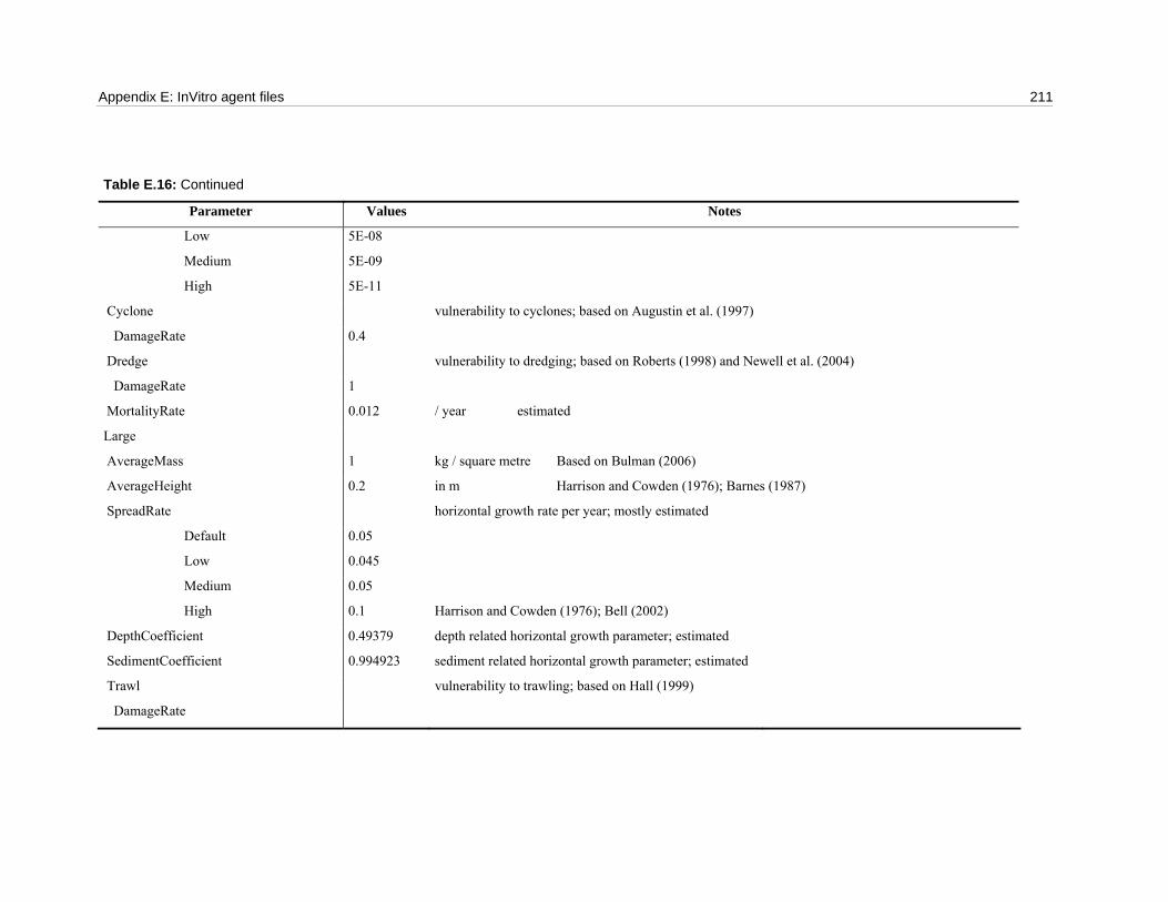
Appendix E: InVitro agent files 211
Table E.16: Continued
Parameter Values Notes
Low 5E-08
Medium 5E-09
High 5E-11
Cyclone vulnerability to cyclones; based on Augustin et al. (1997)
DamageRate 0.4
Dredge vulnerability to dredging; based on Roberts (1998) and Newell et al. (2004)
DamageRate 1
MortalityRate 0.012 / year estimated
Large
AverageMass 1 kg / square metre Based on Bulman (2006)
AverageHeight 0.2 in m Harrison and Cowden (1976); Barnes (1987)
SpreadRate horizontal growth rate per year; mostly estimated
Default 0.05
Low 0.045
Medium 0.05
High 0.1 Harrison and Cowden (1976); Bell (2002)
DepthCoefficient 0.49379 depth related horizontal growth parameter; estimated
SedimentCoefficient 0.994923 sediment related horizontal growth parameter; estimated
Trawl vulnerability to trawling; based on Hall (1999)
DamageRate

212
Table E.16: Continued
Parameter Values Notes
Default 9E-09
Low 9E-08
Medium 9E-09
High 9E-11
Cyclone vulnerability to cyclones; based on Augustin et al. (1997)
DamageRate 0.5
Dredge vulnerability to dredging; based on Roberts (1998) and Newell et al. (2004)
DamageRate 1
MortalityRate 0.0048 / year estimated
SedimentModel 2 set to 0 for shallow-water/hard-bottom growth modified by *SedimentCoefficient to give final growth rates, set to 1 for depth and sediment related expression
ThresholdLongitude 118 longitude in degrees Threshold location for step function in growth and recruitment rates (simplest recruitment model)
ThresholdDepthLeft -100 depth (metres) silt starts to left of threshold longitude
ThresholdDepthRight -160 depth (metres) silt starts to left of threshold longitude
PreferredHabitatName rocky
SuitableHabitatFile sed381.xy.pt
ManmadeHabitat
default 0.05 increment to successful proportion of sedimentatation rate due to manmande habitats
GridedHabitat 0 set this to one if the habitat file is grided data
minimumdepth -10 metres Barnes (1987)
maximumdepth -2000 metres Barnes (1987)
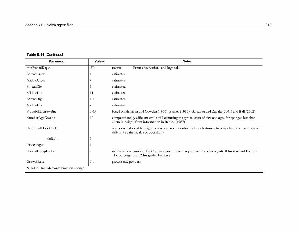
Appendix E: InVitro agent files 213
Table E.16: Continued
Parameter Values Notes
minFishedDepth -50 metres From observations and logbooks
SpreadGrow 1 estimated
MiddleGrow 4 estimated
SpreadDie 1 estimated
MiddleDie 11 estimated
SpreadBig 1.5 estimated
MiddleBig 9 estimated
ProbabilityGrowBig 0.05 based on Harrison and Cowden (1976), Barnes (1987), Garrabou and Zabala (2001) and Bell (2002)
NumberAgeGroups 10 computationally efficient while still capturing the typical span of size and ages for sponges less than 20cm in height, from information in Barnes (1987)
HistoricalEffortCoefft scalar on historical fishing efficiency so no discontinuity from historical to projection treatement (given different spatial scales of operation)
default 1
GridedAgent 1
HabitatComplexity 2 indicates how complex the CSurface environment as percived by other agents: 0 for standard flat grid, 1for polyorganism, 2 for grided benthics
GrowthRate 0.1 growth rate per year
&include Include/contamination-sponge
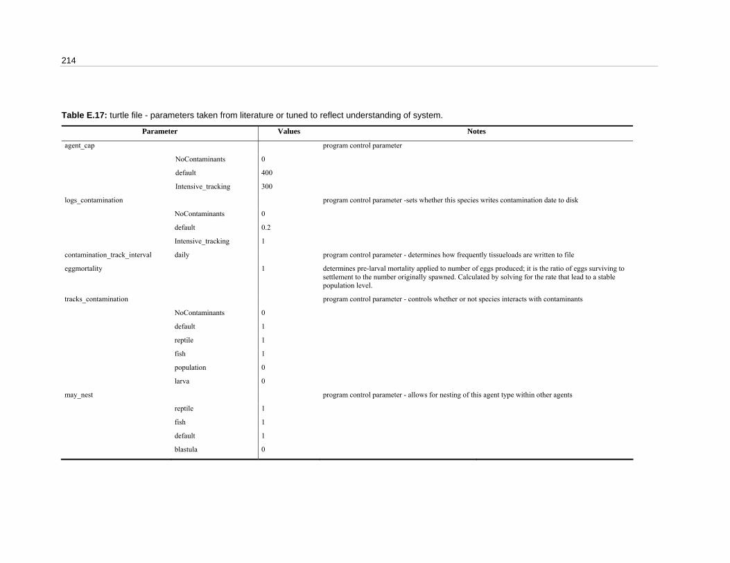
214
Table E.17: turtle file - parameters taken from literature or tuned to reflect understanding of system.
Parameter Values Notes
agent_cap program control parameter
NoContaminants 0
default 400
Intensive_tracking 300
logs_contamination program control parameter -sets whether this species writes contamination date to disk
NoContaminants 0
default 0.2
Intensive_tracking 1
contamination_track_interval daily program control parameter - determines how frequently tissueloads are written to file
eggmortality 1 determines pre-larval mortality applied to number of eggs produced; it is the ratio of eggs surviving to settlement to the number originally spawned. Calculated by solving for the rate that lead to a stable population level.
tracks_contamination program control parameter - controls whether or not species interacts with contaminants
NoContaminants 0
default 1
reptile 1
fish 1
population 0
larva 0
may_nest program control parameter - allows for nesting of this agent type within other agents
reptile 1
fish 1
default 1
blastula 0

Appendix E: InVitro agent files 215
Table E.17: Continued
Parameter Values Notes
cull_period week*4 periodicity of natural mortality (tuned to runtime resolution)
Carrying_capacity 1500000 in kg estimated from Limpus et al. (1984), Marsh and Saalfield (1989), Environment Australia (2000), Chaloupka (2003), Marsh et al. (2004) and Bulman (2006)
Maximum_Age 100 years Limpus and Reed (1985), Chaloupka and Musick (1997), Environment Australia (2000)
t_zero 1 years Age of establishment (maturity in other species, but time when first pulse of mortality drops in the case of turtles; used in mortality calculations); Chaloupka and Musick (1997)
Rate_Mortality
default 0.01 / year Limpus et al. (1994)
highmort 0.05 Chaloupka and Limpus (2002), Chaloupka (2003)
Catastrophic_Mortality 0.03 / event Mortality rate during catastrophic storm event; guesstimate based on Chaloupka (2003)
Speed 0.02 metres / second cruising speed from FISHBASE (2005)
MaxSpeed 0.05 metres / second from FISHBASE (2005)
SearchRadiusExponent 4 governs how far afield we assume organisms can detect conditions (estimated on velocity)
Directional_variability 0.8 degree to which they remain moving in a single facing (direction); calibrated
Speed_variability 0.07 stochastic variability in wandering speed; calculated by comparing crusing and maximum speeds in Eckert (2002)
Traverse_Time 0.1 months Time taken to cross the entire NWS if swimming directly; calculated from swimming speed, weighted by degree of aggregation (of agent – so populations took longer than fish)
Length/Mass 0.5 estimated
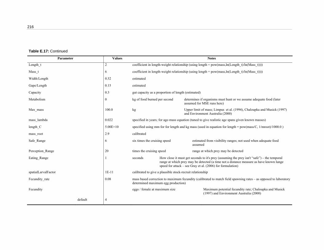
216
Table E.17: Continued
Parameter Values Notes
Length_t 2 coefficient in length-weight relationship (using length = pow(mass,ln(Length_t)/ln(Mass_t))))
Mass_t 6 coefficient in length-weight relationship (using length = pow(mass,ln(Length_t)/ln(Mass_t))))
Width/Length 0.52 estimated
Gape/Length 0.15 estimated
Capacity 0.3 gut capacity as a proportion of length (estimated)
Metabolism 0 kg of food burned per second determines if organisms must hunt or we assume adequate food (later assumed for MSE runs here)
Max_mass 100.0 kg Upper limit of mass; Limpus et al. (1994), Chaloupka and Musick (1997) and Environment Australia (2000)
mass_lambda 0.022 specified in years; for age-mass equation (tuned to give realistic age spans given known masses)
length_C 5.00E+10 specified using mm for for length and kg mass (used in equation for length = pow(mass/C, 1/mroot)/1000.0 )
mass_root 2.9 calibrated
Safe_Range 6 six times the cruising speed estimated from visibility ranges; not used when adequate food assumed
Perception_Range 20 times the cruising speed range at which prey may be detected
Eating_Range 1 seconds How close it must get seconds to it's prey (assuming the prey isn't “safe”) – the temporal range at which prey may be detected (a time not a distance measure as have known lunge speed for attack – see Gray et al. (2006) for formulation)
spatialLarvalFactor 1E-11 calibrated to give a plausible stock-recruit relationship
Fecundity_rate 0.08 mass based correction to maximum fecundity (calibrated to match field spawning rates – as opposed to laboratory determined maximum egg production)
Fecundity eggs / female at maximum size Maximum potential fecundity rate; Chaloupka and Musick (1997) and Environment Australia (2000)
default 4
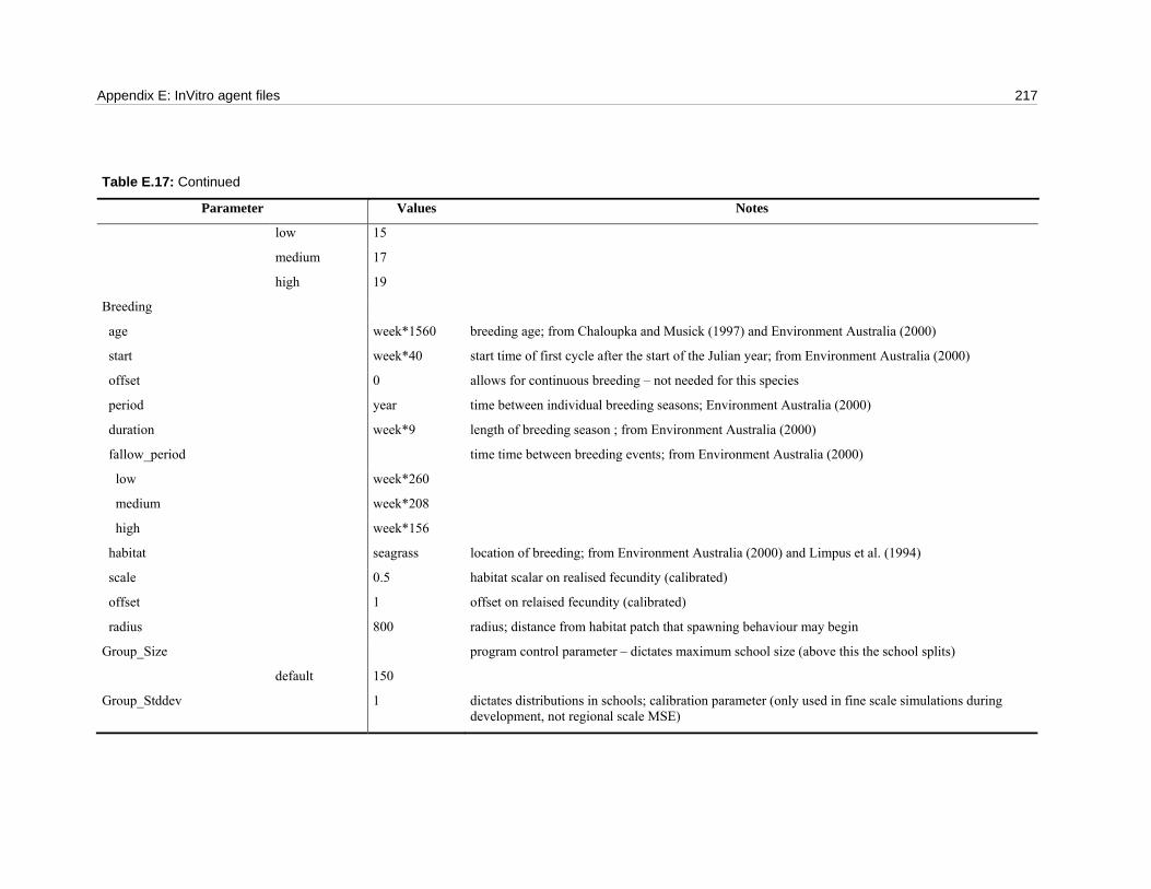
Appendix E: InVitro agent files 217
Table E.17: Continued
Parameter Values Notes
low 15
medium 17
high 19
Breeding
age week*1560 breeding age; from Chaloupka and Musick (1997) and Environment Australia (2000)
start week*40 start time of first cycle after the start of the Julian year; from Environment Australia (2000)
offset 0 allows for continuous breeding – not needed for this species
period year time between individual breeding seasons; Environment Australia (2000)
duration week*9 length of breeding season ; from Environment Australia (2000)
fallow_period time time between breeding events; from Environment Australia (2000)
low week*260
medium week*208
high week*156
habitat seagrass location of breeding; from Environment Australia (2000) and Limpus et al. (1994)
scale 0.5 habitat scalar on realised fecundity (calibrated)
offset 1 offset on relaised fecundity (calibrated)
radius 800 radius; distance from habitat patch that spawning behaviour may begin
Group_Size program control parameter – dictates maximum school size (above this the school splits)
default 150
Group_Stddev 1 dictates distributions in schools; calibration parameter (only used in fine scale simulations during development, not regional scale MSE)
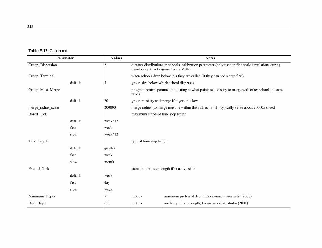
218
Table E.17: Continued
Parameter Values Notes
Group_Dispersion 2 dictates distributions in schools; calibration parameter (only used in fine scale simulations during development, not regional scale MSE)
Group_Terminal when schools drop below this they are culled (if they can not merge first)
default 5 group size below which school disperses
Group_Must_Merge program control parameter dictating at what points schools try to merge with other schools of same taxon
default 20 group must try and merge if it gets this low
merge_radius_scale 200000 merge radius (to merge must be within this radius in m) – typically set to about 20000x speed
Bored_Tick maximum standard time step length
default week*12
fast week
slow week*12
Tick_Length typical time step length
default quarter
fast week
slow month
Excited_Tick standard time step length if in active state
default week
fast day
slow week
Minimum_Depth 5 metres minimum preferred depth; Environment Australia (2000)
Best_Depth -50 metres median preferred depth; Environment Australia (2000)

Appendix E: InVitro agent files 219
Table E.17: Continued
Parameter Values Notes
Maximum_Depth -550 metres maximum preferred depth; Environment Australia (2000)
Minimum_Sea_Depth -1 metres minimum depth typically used in marine waters (used to constrain locations in scenarios)
Maximum_Sea_Depth -6000 metres maximum depth typically reached in marine waters (often used to constrain the populations to specific locations for fine scale simulations)
radius 4000 metres school extent
BycatchSpecies 1 if set1 then will be depleted by historical fishing (via incidental mortality)
trawl_efficiency efficiency of trawlers against species (based on sharks)
default 0.1 analogous to selectivity in the populations file
low 0.45 very susceptible to trawling
medium 0.35
high 0.3 can avoid trawls
HistoricalEffortCoefft 0.006 calibrated so that predicted catch of turtles matches observations (Prince pers. comm.; WA Fisheries)
spatialCatchFact 5.00E-09 calibrated to minimise differences between observed and predicted catches
selMass 1 kg mass juveniles when first susceptible to fishing (estimated)
assess_environment 1 flag to show whether species seeks favourable environments
Awareness_type 1 0 for fine scale awareness, 1 for large scale program control parameter – dictating resolution of adviser agent interrogation (see Gray et al. (2006))
ScalingBestSeaDepth Weighting for influence of preferred depth in guiding habitat selection
default 0.0001 Weighting for influence of preferred depth in guiding habitat selection
Mass0 0.4 kg mass of individual turtle hatchlings; based on Environment Australia (2000) and Chaloupka (2003)
Larva juvenile parameters
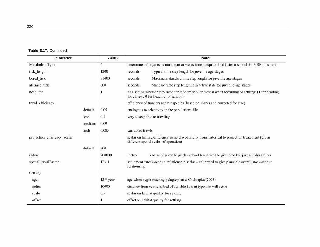
220
Table E.17: Continued
Parameter Values Notes
MetabolismType 4 determines if organisms must hunt or we assume adequate food (later assumed for MSE runs here)
tick_length 1200 seconds Typical time step length for juvenile age stages
bored_tick 81400 seconds Maximum standard time step length for juvenile age stages
alarmed_tick 600 seconds Standard time step length if in active state for juvenile age stages
head_for 1 flag setting whether they head for random spot or closest when recruiting or settling: (1 for heading for closest, 0 for heading for random)
trawl_efficiency efficiency of trawlers against species (based on sharks and corrected for size)
default 0.05 analogous to selectivity in the populations file
low 0.1 very susceptible to trawling
medium 0.09
high 0.085 can avoid trawls
projection_efficiency_scalar scalar on fishing efficiency so no discontinuity from historical to projection treatement (given different spatial scales of operation)
default 200
radius 200000 metres Radius of juvenile patch / school (calibrated to give credible juvenile dynamics)
spatialLarvalFactor 1E-11 settlement “stock-recruit” relationship scalar – calibrated to give plausible overall stock-recruit relationship
Settling
age 13 * year age when begin entering pelagic phase; Chaloupka (2003)
radius 10000 distance from centre of bed of suitable habitat type that will settle
scale 0.5 scalar on habitat quality for settling
offset 1 offset on habitat quality for settling
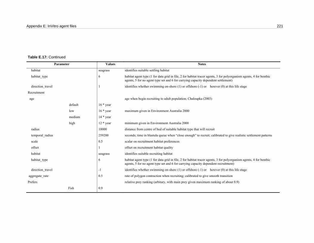
Appendix E: InVitro agent files 221
Table E.17: Continued
Parameter Values Notes
habitat seagrass identifies suitable settling habitat
habitat_type 6 habitat agent type (1 for data grid in file, 2 for habitat tracer agents, 3 for polyorganism agents, 4 for benthic agents, 5 for no agent type set and 6 for carrying capacity dependent settlement)
direction_travel 1 identifies whether swimming on-shore (1) or offshore (-1) or �herever (0) at this life stage
Recruitment
age age when begin recruiting to adult population; Chaloupka (2003)
default 16 * year
low 16 * year maximum given in Environment Australia 2000
medium 14 * year
high 12 * year minimum given in Environment Australia 2000
radius 10000 distance from centre of bed of suitable habitat type that will recruit
temporal_radius 259200 seconds; time in blastula queue when “close enough” to recruit; calibrated to give realistic settlement patterns
scale 0.5 scalar on recruitment habitat preferences
offset 1 offset on recruitment habitat quality
habitat seagrass identifies suitable recruiting habitat
habitat_type 6 habitat agent type (1 for data grid in file, 2 for habitat tracer agents, 3 for polyorganism agents, 4 for benthic agents, 5 for no agent type set and 6 for carrying capacity dependent recruitment)
direction_travel -1 identifies whether swimming on-shore (1) or offshore (-1) or �herever (0) at this life stage
aggregate_rate 0.5 rate of polygon contraction when recruiting; calibrated to give smooth transition
Prefers relative prey ranking (arbitary, with main prey given maximum ranking of about 0.9)
Fish 0.9

222
Table E.17: Continued
Parameter Values Notes
benthos 0.9
Fears relative fear ranking (arbitary, with main predators given maximum ranking of about 0.9)
Shark 0.9
Habitat relative adult habitat ranking (arbitary, with most preferred habitat given maximum ranking of about 0.9)
Seagrass 0.5
Seagrass_thresh 10649880 total biomass (kg) in habitat grid cell; threshold biomass below which the animal is less interested in the habitat
&include Include/contamination-finfish
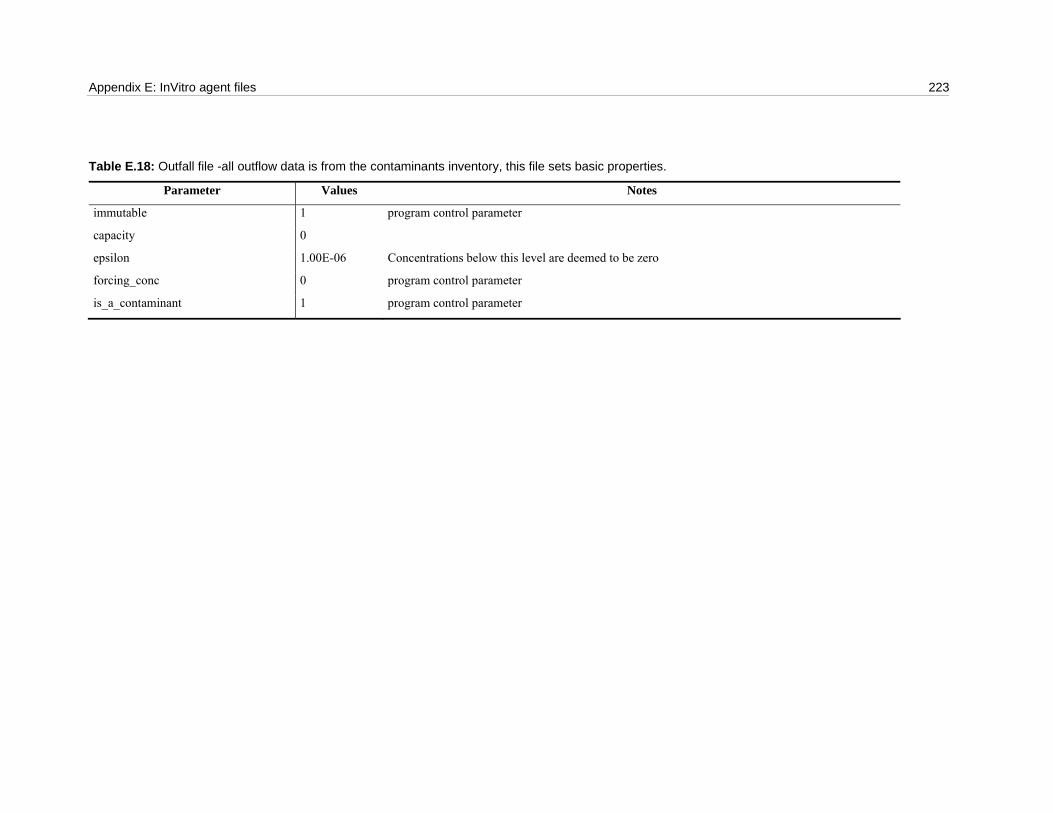
Appendix E: InVitro agent files 223
Table E.18: Outfall file -all outflow data is from the contaminants inventory, this file sets basic properties.
Parameter Values Notes
immutable 1 program control parameter
capacity 0
epsilon 1.00E-06 Concentrations below this level are deemed to be zero
forcing_conc 0 program control parameter
is_a_contaminant 1 program control parameter
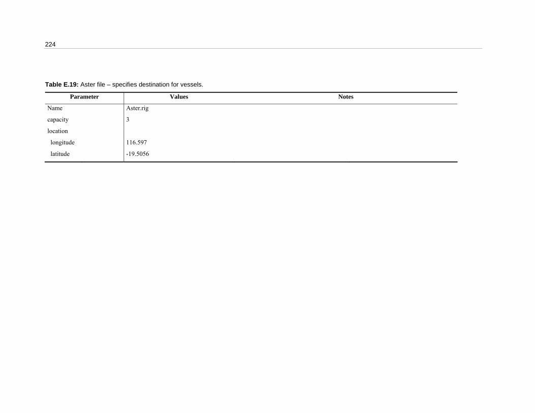
224
Table E.19: Aster file – specifies destination for vessels.
Parameter Values Notes
Name Aster.rig
capacity 3
location
longitude 116.597
latitude -19.5056
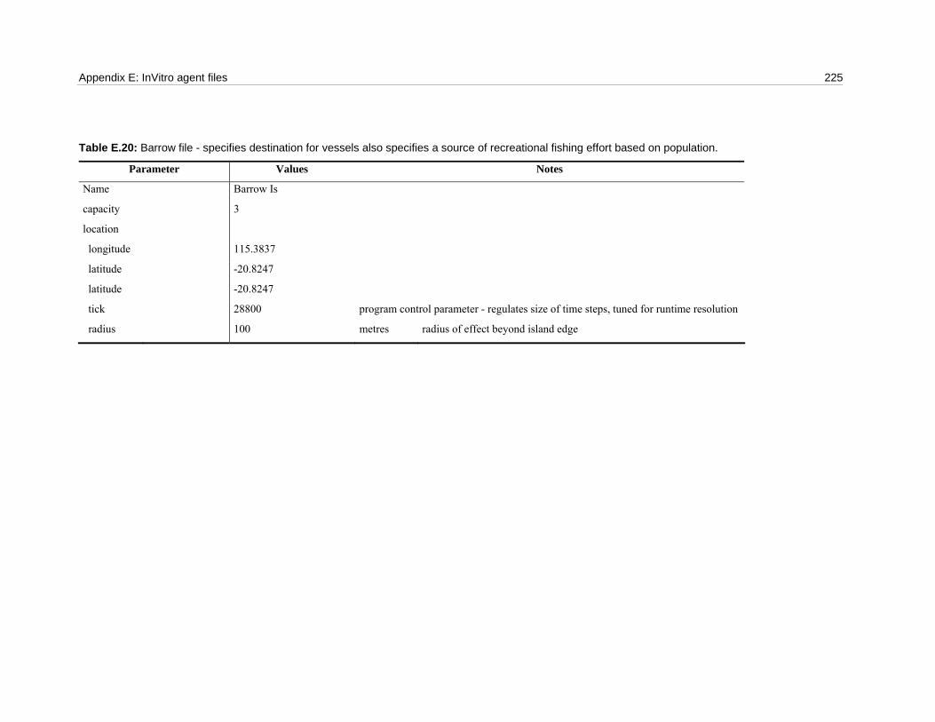
Appendix E: InVitro agent files 225
Table E.20: Barrow file - specifies destination for vessels also specifies a source of recreational fishing effort based on population.
Parameter Values Notes
Name Barrow Is
capacity 3
location
longitude 115.3837
latitude -20.8247
latitude -20.8247
tick 28800 program control parameter - regulates size of time steps, tuned for runtime resolution
radius 100 metres radius of effect beyond island edge
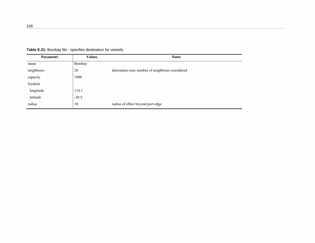
226
Table E.21: Bombay file - specifies destination for vessels.
Parameter Values Notes
name Bombay
neighbours 20 determines max number of neighbours considered
capacity 1000
location
longitude 114.1
latitude -20.5
radius 10 radius of effect beyond port edge

Appendix E: InVitro agent files 227
Table E.22: Calcutta file - specifies destination for vessels.
Parameter Values Notes
name Calcutta
capacity 1000
location
longitude 114.5
latitude -17.5
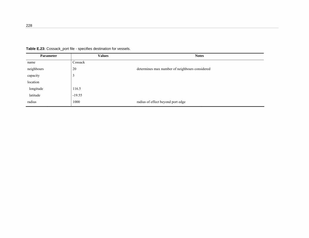
228
Table E.23: Cossack_port file - specifies destination for vessels.
Parameter Values Notes
name Cossack
neighbours 20 determines max number of neighbours considered
capacity 3
location
longitude 116.5
latitude -19.55
radius 1000 radius of effect beyond port edge
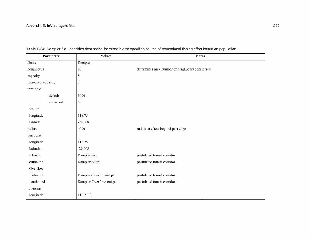
Appendix E: InVitro agent files 229
Table E.24: Dampier file - specifies destination for vessels also specifies source of recreational fishing effort based on population.
Parameter Values Notes
Name Dampier
neighbours 20 determines max number of neighbours considered
capacity 5
increased_capacity 2
threshold
default 1000
enhanced 50
location
longitude 116.75
latitude -20.608
radius 4000 radius of effect beyond port edge
waypoint
longitude 116.75
latitude -20.608
inbound Dampier-in.pt postulated transit corridor
outbound Dampier-out.pt postulated transit corridor
Overflow
inbound Dampier-Overflow-in.pt postulated transit corridor
outbound Dampier-Overflow-out.pt postulated transit corridor
township
longitude 116.7133

230
Table E.24: Continued
Parameter Values Notes
latitude -20.66
price prices for commodities (spot prices, not kept up to date)
fuel 1.2
Shark 12
Fish 7
forcing_invoked program control parameter - selects development scenario
default 0
1p 1
2p 2
forcing_system program control parameter - selects timeseries to be used
population Dampier-pop.ts
population1p Dampier-pop-1p.ts
population2p Dampier-pop-2p.ts
production Dampier-prod.ts
production1p Dampier-prod-1p.ts
production2p Dampier-prod-2p.ts
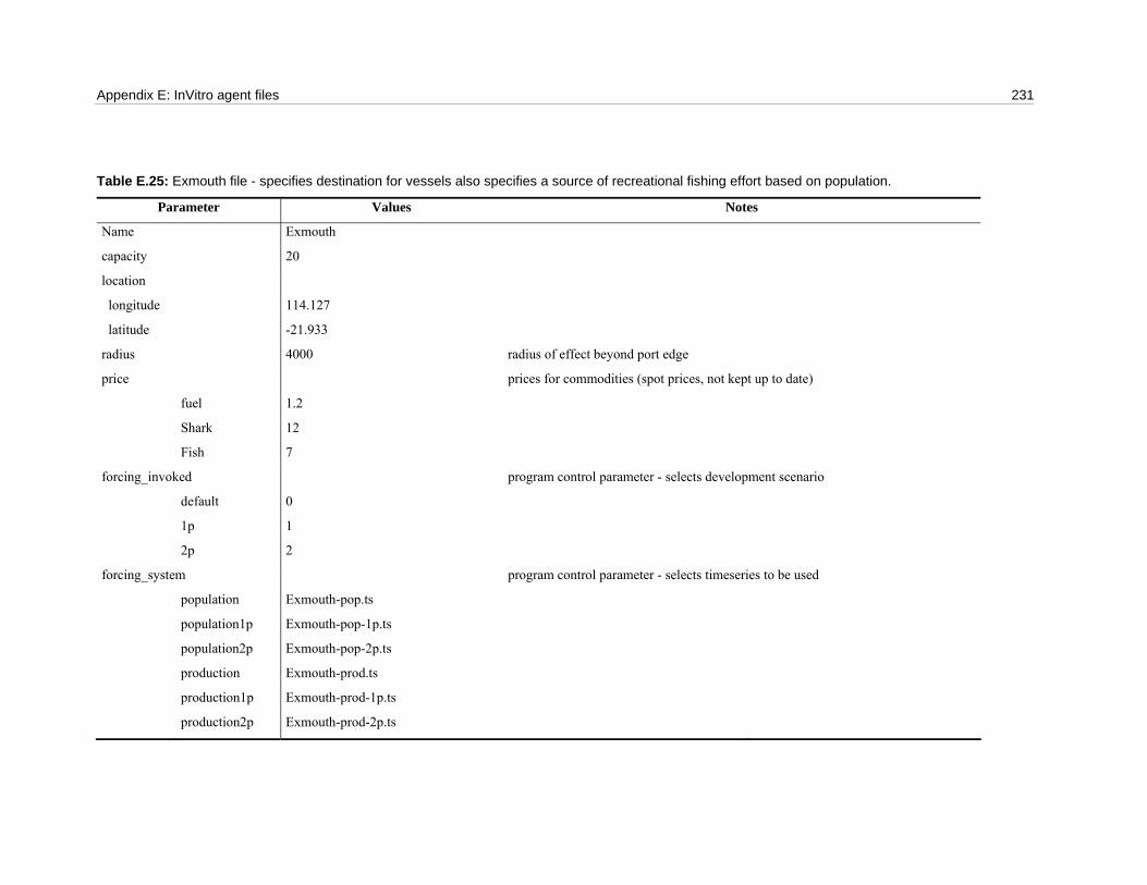
Appendix E: InVitro agent files 231
Table E.25: Exmouth file - specifies destination for vessels also specifies a source of recreational fishing effort based on population.
Parameter Values Notes
Name Exmouth
capacity 20
location
longitude 114.127
latitude -21.933
radius 4000 radius of effect beyond port edge
price prices for commodities (spot prices, not kept up to date)
fuel 1.2
Shark 12
Fish 7
forcing_invoked program control parameter - selects development scenario
default 0
1p 1
2p 2
forcing_system program control parameter - selects timeseries to be used
population Exmouth-pop.ts
population1p Exmouth-pop-1p.ts
population2p Exmouth-pop-2p.ts
production Exmouth-prod.ts
production1p Exmouth-prod-1p.ts
production2p Exmouth-prod-2p.ts
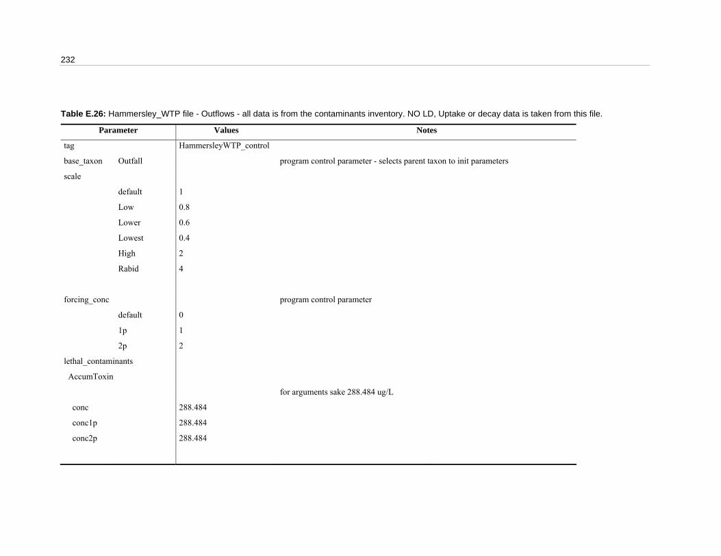
232
Table E.26: Hammersley_WTP file - Outflows - all data is from the contaminants inventory. NO LD, Uptake or decay data is taken from this file.
Parameter Values Notes
tag HammersleyWTP_control
base_taxon Outfall program control parameter - selects parent taxon to init parameters
scale
default 1
Low 0.8
Lower 0.6
Lowest 0.4
High 2
Rabid 4
forcing_conc program control parameter
default 0
1p 1
2p 2
lethal_contaminants
AccumToxin
for arguments sake 288.484 ug/L
conc 288.484
conc1p 288.484
conc2p 288.484
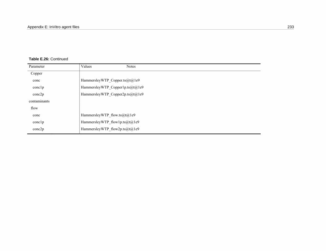
Appendix E: InVitro agent files 233
Table E.26: Continued
Parameter Values Notes
Copper
conc HammersleyWTP_Copper.ts@t@1e9
conc1p HammersleyWTP_Copper1p.ts@t@1e9
conc2p HammersleyWTP_Copper2p.ts@t@1e9
contaminants
flow
conc HammersleyWTP_flow.ts@t@1e9
conc1p HammersleyWTP_flow1p.ts@t@1e9
conc2p HammersleyWTP_flow2p.ts@t@1e9
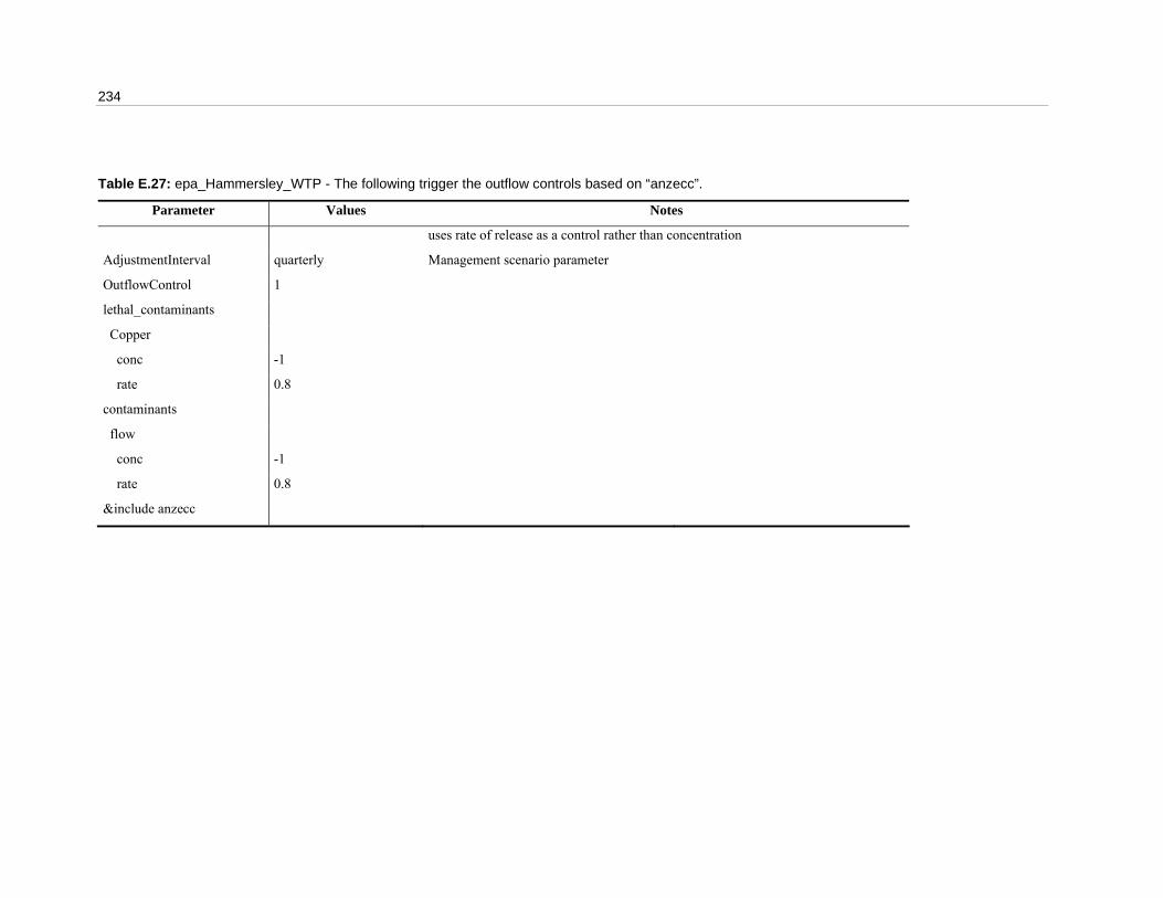
234
Table E.27: epa_Hammersley_WTP - The following trigger the outflow controls based on “anzecc”.
Parameter Values Notes
uses rate of release as a control rather than concentration
AdjustmentInterval quarterly Management scenario parameter
OutflowControl 1
lethal_contaminants
Copper
conc -1
rate 0.8
contaminants
flow
conc -1
rate 0.8
&include anzecc
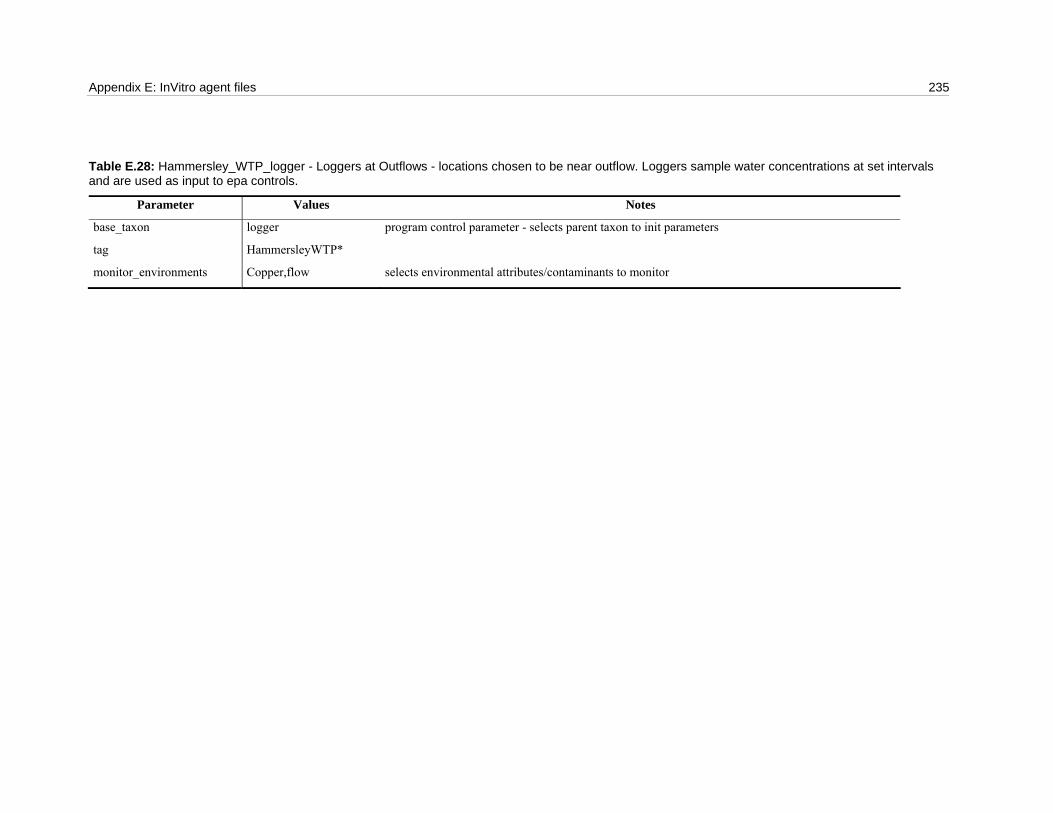
Appendix E: InVitro agent files 235
Table E.28: Hammersley_WTP_logger - Loggers at Outflows - locations chosen to be near outflow. Loggers sample water concentrations at set intervals and are used as input to epa controls.
Parameter Values Notes
base_taxon logger program control parameter - selects parent taxon to init parameters
tag HammersleyWTP*
monitor_environments Copper,flow selects environmental attributes/contaminants to monitor
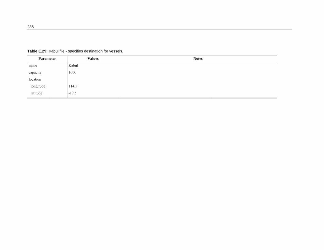
236
Table E.29: Kabul file - specifies destination for vessels.
Parameter Values Notes
name Kabul
capacity 1000
location
longitude 114.5
latitude -17.5
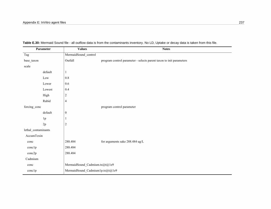
Appendix E: InVitro agent files 237
Table E.30: Mermaid Sound file - all outflow data is from the contaminants inventory. No LD, Uptake or decay data is taken from this file.
Parameter Values Notes
Tag MermaidSound_control
base_taxon Outfall program control parameter - selects parent taxon to init parameters
scale
default 1
Low 0.8
Lower 0.6
Lowest 0.4
High 2
Rabid 4
forcing_conc program control parameter
default 0
1p 1
2p 2
lethal_contaminants
AccumToxin
conc 288.484 for arguments sake 288.484 ug/L
conc1p 288.484
conc2p 288.484
Cadmium
conc MermaidSound_Cadmium.ts@t@1e9
conc1p MermaidSound_Cadmium1p.ts@t@1e9
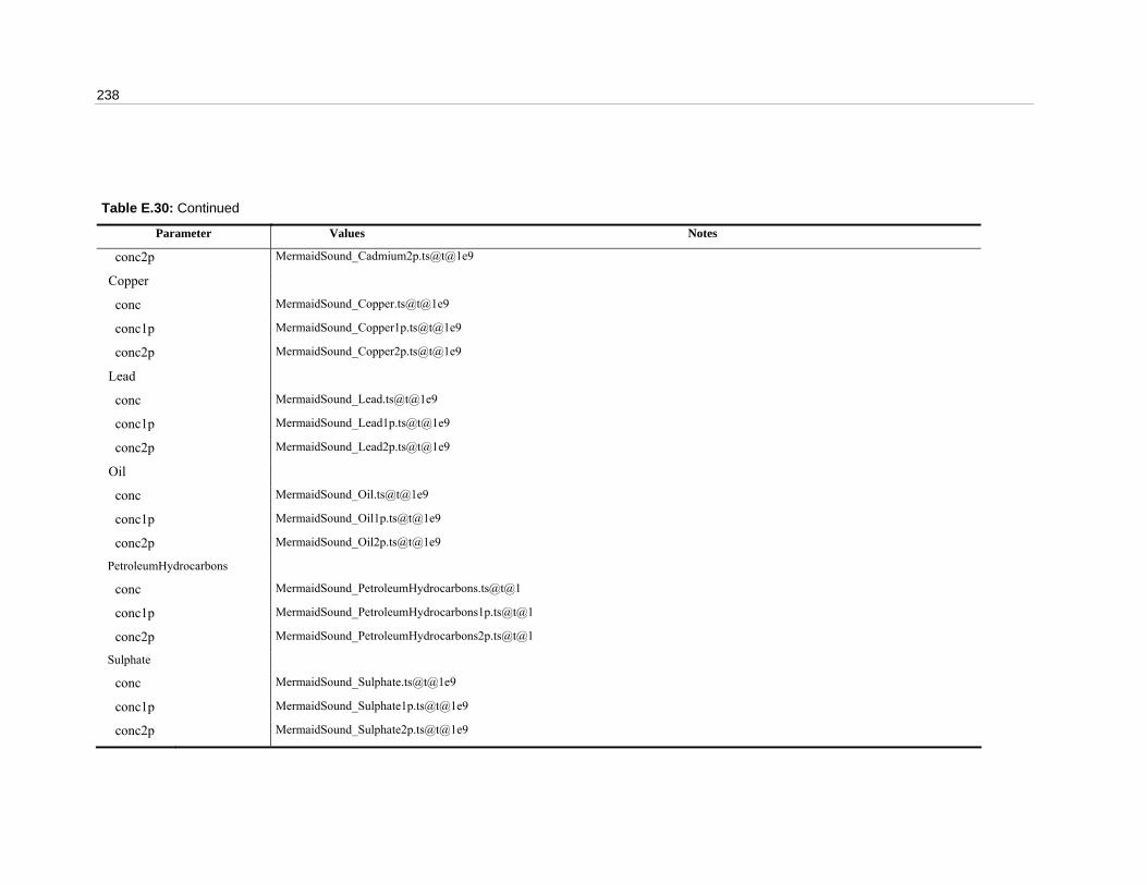
238
Table E.30: Continued
Parameter Values Notes
conc2p MermaidSound_Cadmium2p.ts@t@1e9
Copper
conc MermaidSound_Copper.ts@t@1e9
conc1p MermaidSound_Copper1p.ts@t@1e9
conc2p MermaidSound_Copper2p.ts@t@1e9
Lead
conc MermaidSound_Lead.ts@t@1e9
conc1p MermaidSound_Lead1p.ts@t@1e9
conc2p MermaidSound_Lead2p.ts@t@1e9
Oil
conc MermaidSound_Oil.ts@t@1e9
conc1p MermaidSound_Oil1p.ts@t@1e9
conc2p MermaidSound_Oil2p.ts@t@1e9
PetroleumHydrocarbons
conc MermaidSound_PetroleumHydrocarbons.ts@t@1
conc1p MermaidSound_PetroleumHydrocarbons1p.ts@t@1
conc2p MermaidSound_PetroleumHydrocarbons2p.ts@t@1
Sulphate
conc MermaidSound_Sulphate.ts@t@1e9
conc1p MermaidSound_Sulphate1p.ts@t@1e9
conc2p MermaidSound_Sulphate2p.ts@t@1e9
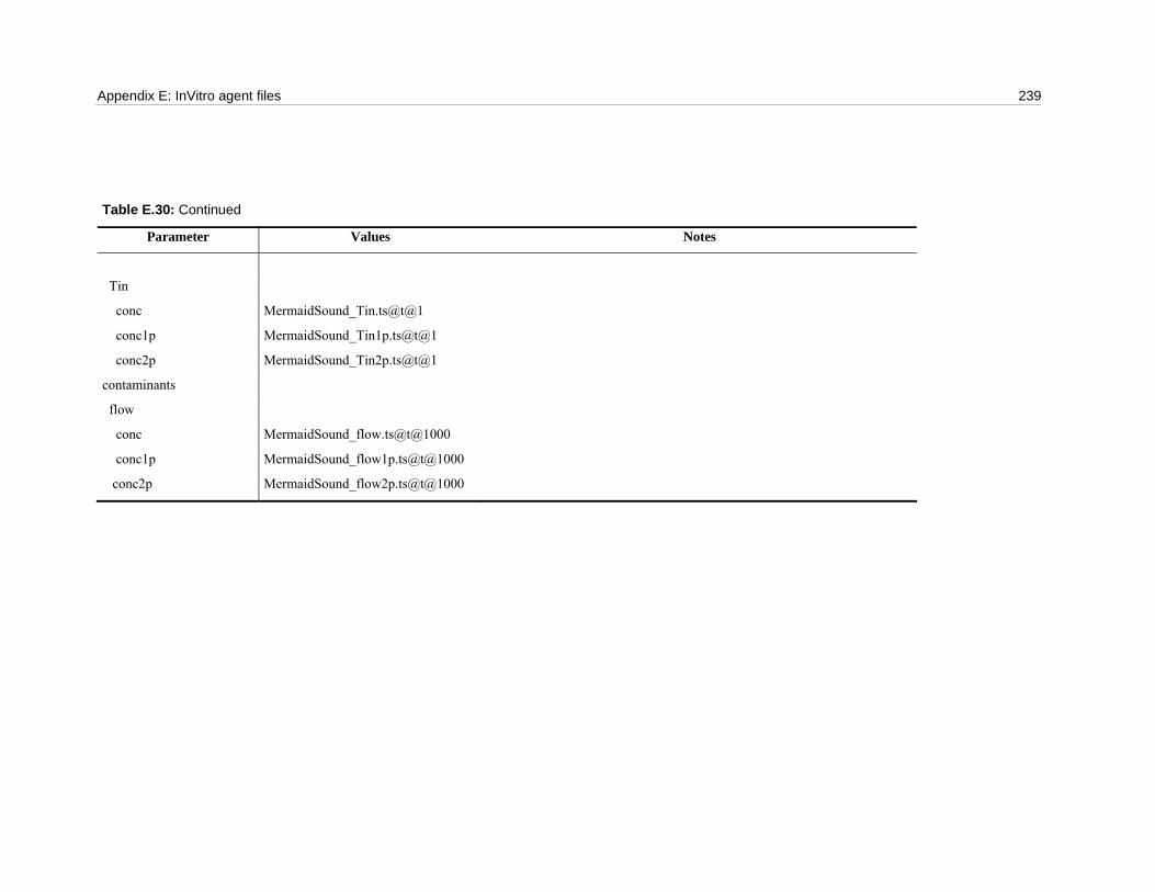
Appendix E: InVitro agent files 239
Table E.30: Continued
Parameter Values Notes
Tin
conc MermaidSound_Tin.ts@t@1
conc1p MermaidSound_Tin1p.ts@t@1
conc2p MermaidSound_Tin2p.ts@t@1
contaminants
flow
conc MermaidSound_flow.ts@t@1000
conc1p MermaidSound_flow1p.ts@t@1000
conc2p MermaidSound_flow2p.ts@t@1000
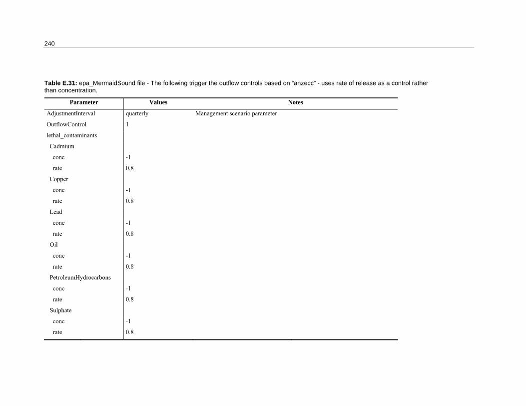
240
Table E.31: epa_MermaidSound file - The following trigger the outflow controls based on “anzecc” - uses rate of release as a control rather than concentration.
Parameter Values Notes
AdjustmentInterval quarterly Management scenario parameter
OutflowControl 1
lethal_contaminants
Cadmium
conc -1
rate 0.8
Copper
conc -1
rate 0.8
Lead
conc -1
rate 0.8
Oil
conc -1
rate 0.8
PetroleumHydrocarbons
conc -1
rate 0.8
Sulphate
conc -1
rate 0.8
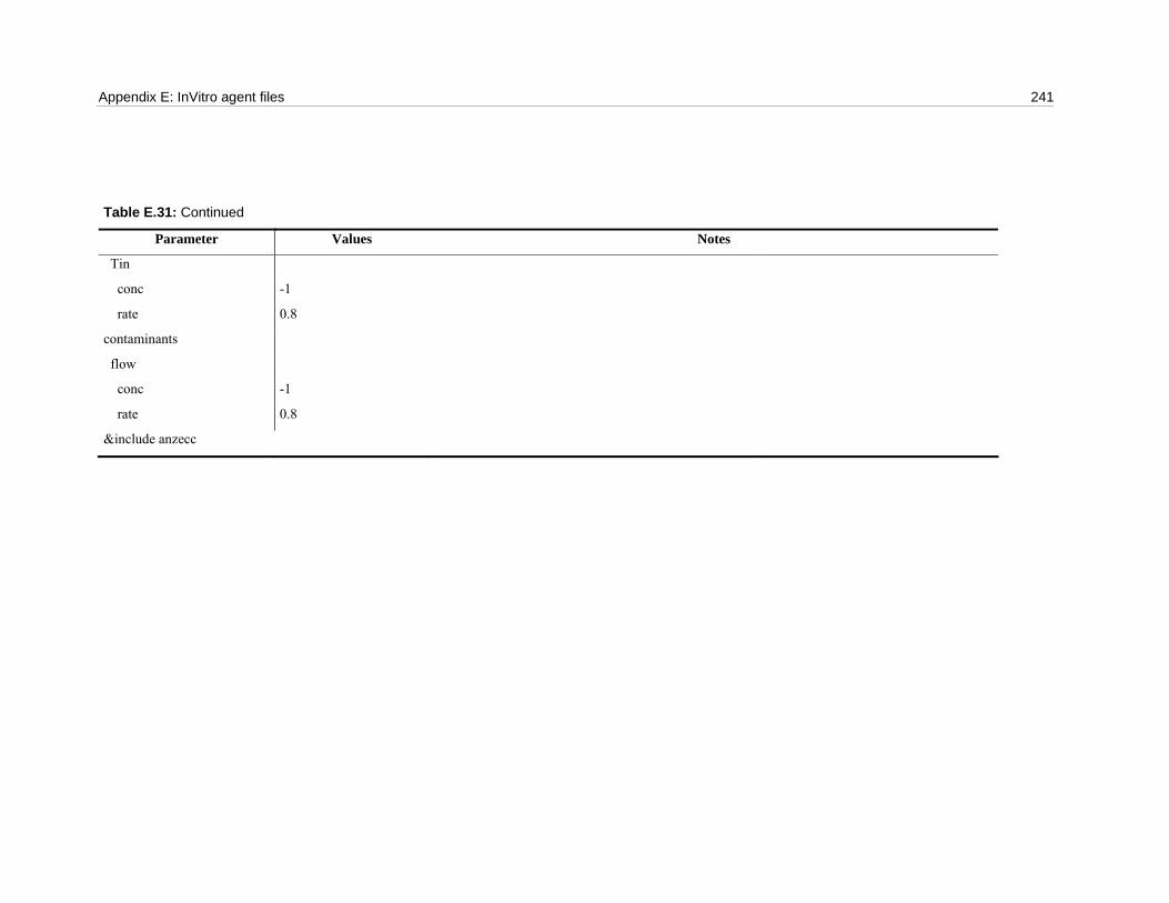
Appendix E: InVitro agent files 241
Table E.31: Continued
Parameter Values Notes
Tin
conc -1
rate 0.8
contaminants
flow
conc -1
rate 0.8
&include anzecc

242
Table E.32: MermaidSound_loggerfile - Loggers at Outflows - locations chosen to be near outflow. Loggers sample water concentrations at set intervals and are used as input to epa controls.
Parameter Values Notes
base_taxon logger program control parameter - selects parent taxon to init parameters
tag MermaidSound*
monitor_environments Cadmium, Copper, Lead, Oil, PetroleumHydrocarbons, Sulphate, Tin, flow
selects environmental attributes/contaminants to monitor

Appendix E: InVitro agent files 243
Table E.33: NRA_port file - specifies destination for vessels.
Parameter Values Notes
name North Rankin A
neighbours 20 determines max number of neighbours considered
capacity 3
location
longitude 116.15
latitude -19.5
radius 1000 radius of effect beyond platform edge
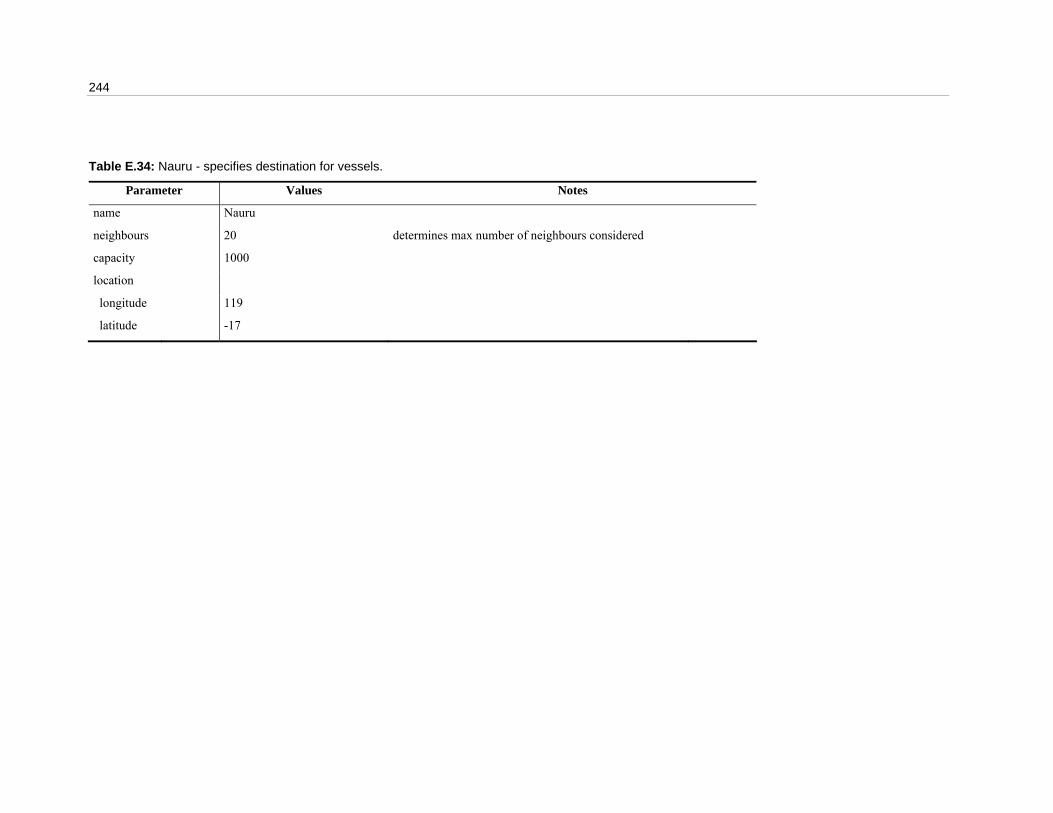
244
Table E.34: Nauru - specifies destination for vessels.
Parameter Values Notes
name Nauru
neighbours 20 determines max number of neighbours considered
capacity 1000
location
longitude 119
latitude -17
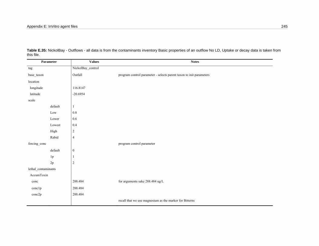
Appendix E: InVitro agent files 245
Table E.35: NickolBay - Outflows - all data is from the contaminants inventory Basic properties of an outflow No LD, Uptake or decay data is taken from this file.
Parameter Values Notes
tag NickolBay_control
base_taxon Outfall program control parameter - selects parent taxon to init parameters
location
longitude 116.8147
latitude -20.6954
scale
default 1
Low 0.8
Lower 0.6
Lowest 0.4
High 2
Rabid 4
forcing_conc program control parameter
default 0
1p 1
2p 2
lethal_contaminants
AccumToxin
conc 288.484 for arguments sake 288.484 ug/L
conc1p 288.484
conc2p 288.484
recall that we use magnesium as the marker for Bitterns
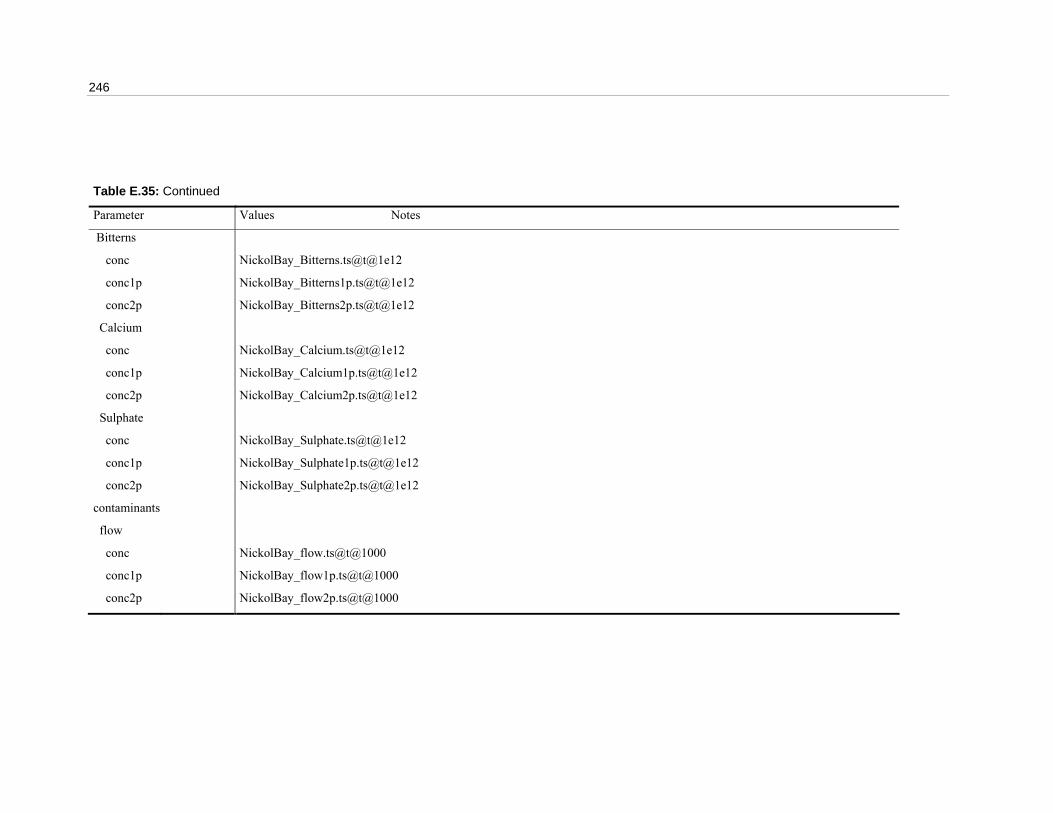
246
Table E.35: Continued
Parameter Values Notes
Bitterns
conc NickolBay_Bitterns.ts@t@1e12
conc1p NickolBay_Bitterns1p.ts@t@1e12
conc2p NickolBay_Bitterns2p.ts@t@1e12
Calcium
conc NickolBay_Calcium.ts@t@1e12
conc1p NickolBay_Calcium1p.ts@t@1e12
conc2p NickolBay_Calcium2p.ts@t@1e12
Sulphate
conc NickolBay_Sulphate.ts@t@1e12
conc1p NickolBay_Sulphate1p.ts@t@1e12
conc2p NickolBay_Sulphate2p.ts@t@1e12
contaminants
flow
conc NickolBay_flow.ts@t@1000
conc1p NickolBay_flow1p.ts@t@1000
conc2p NickolBay_flow2p.ts@t@1000

Appendix E: InVitro agent files 247
Table E.36: epa_NickolBay file - The following trigger the outflow controls based on “anzecc” uses rate of release as a control rather than concentration.
Parameter Values Notes
AdjustmentInterval quarterly management scenario parameter
OutflowControl 1
lethal_contaminants
Bitterns
conc -1
rate 0.8
Calcium
conc -1
rate 0.8
Sulphate
conc -1
rate 0.8
contaminants
flow
conc -1
rate 0.8
&include anzecc
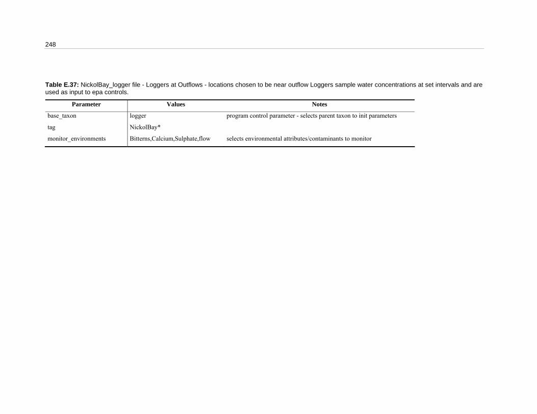
248
Table E.37: NickolBay_logger file - Loggers at Outflows - locations chosen to be near outflow Loggers sample water concentrations at set intervals and are used as input to epa controls.
Parameter Values Notes
base_taxon logger program control parameter - selects parent taxon to init parameters
tag NickolBay*
monitor_environments Bitterns,Calcium,Sulphate,flow selects environmental attributes/contaminants to monitor
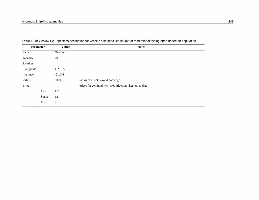
Appendix E: InVitro agent files 249
Table E.38: Onslow file - specifies destination for vessels also specifies source of recreational fishing effort based on population.
Parameter Values Notes
name Onslow
capacity 20
location
longitude 115.135
latitude -21.688
radius 3000 radius of effect beyond port edge
price prices for commodities (spot prices, not kept up to date)
fuel 1.2
Shark 12
Fish 7

250
Table E.39: Osaka file - specifies destination for vessels.
Parameter Values Notes
name Osaka
neighbours 20 Determines max number of neighbours considered
capacity 1000
location
longitude 117.21
latitude -17.5
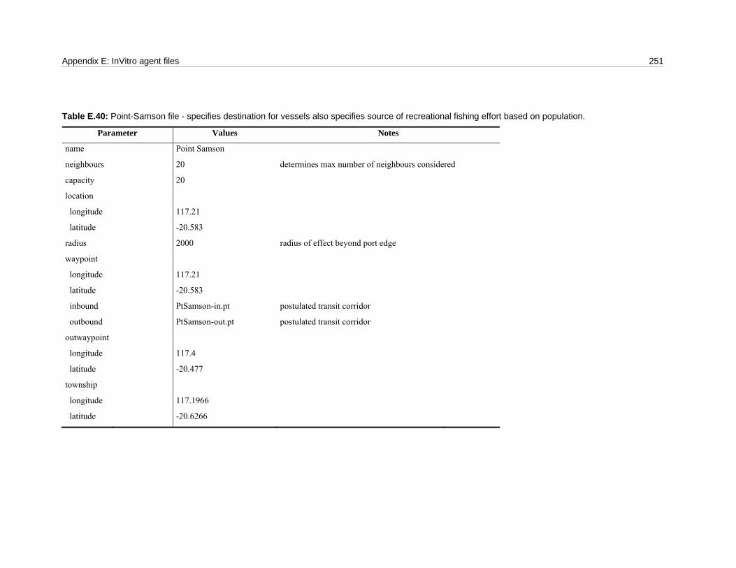
Appendix E: InVitro agent files 251
Table E.40: Point-Samson file - specifies destination for vessels also specifies source of recreational fishing effort based on population.
Parameter Values Notes
name Point Samson
neighbours 20 determines max number of neighbours considered
capacity 20
location
longitude 117.21
latitude -20.583
radius 2000 radius of effect beyond port edge
waypoint
longitude 117.21
latitude -20.583
inbound PtSamson-in.pt postulated transit corridor
outbound PtSamson-out.pt postulated transit corridor
outwaypoint
longitude 117.4
latitude -20.477
township
longitude 117.1966
latitude -20.6266
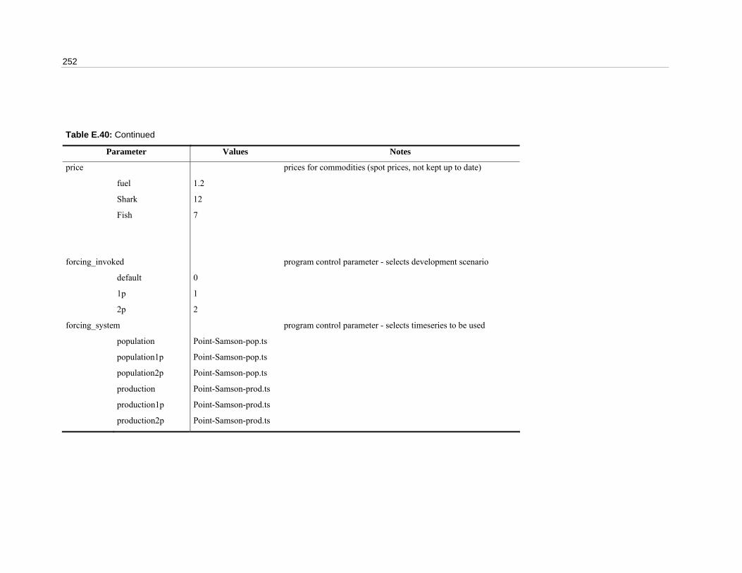
252
Table E.40: Continued
Parameter Values Notes
price prices for commodities (spot prices, not kept up to date)
fuel 1.2
Shark 12
Fish 7
forcing_invoked program control parameter - selects development scenario
default 0
1p 1
2p 2
forcing_system program control parameter - selects timeseries to be used
population Point-Samson-pop.ts
population1p Point-Samson-pop.ts
population2p Point-Samson-pop.ts
production Point-Samson-prod.ts
production1p Point-Samson-prod.ts
production2p Point-Samson-prod.ts
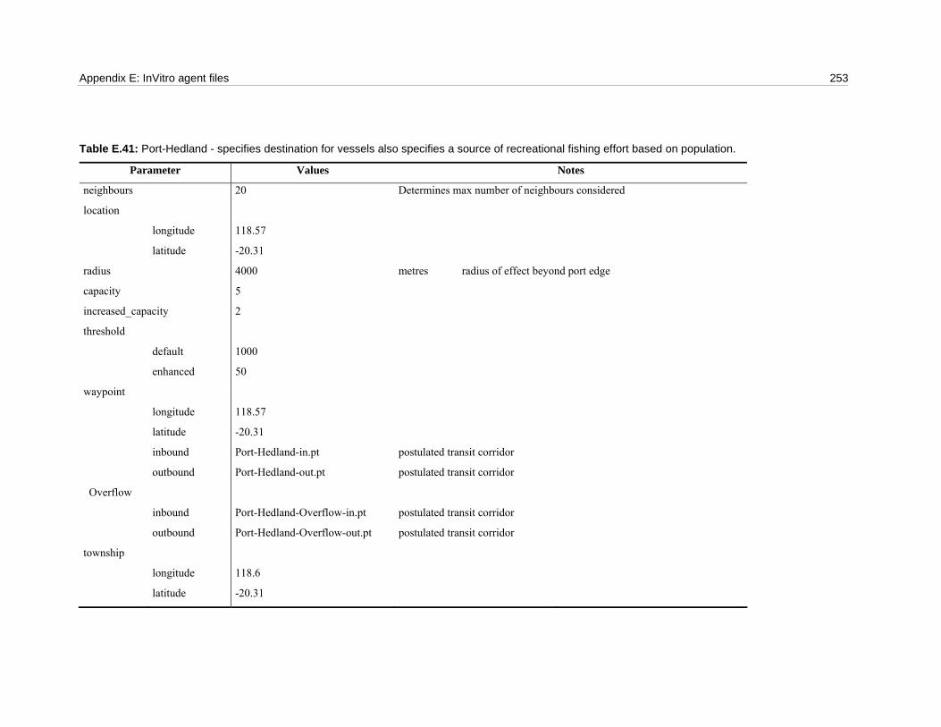
Appendix E: InVitro agent files 253
Table E.41: Port-Hedland - specifies destination for vessels also specifies a source of recreational fishing effort based on population.
Parameter Values Notes
neighbours 20 Determines max number of neighbours considered
location
longitude 118.57
latitude -20.31
radius 4000 metres radius of effect beyond port edge
capacity 5
increased_capacity 2
threshold
default 1000
enhanced 50
waypoint
longitude 118.57
latitude -20.31
inbound Port-Hedland-in.pt postulated transit corridor
outbound Port-Hedland-out.pt postulated transit corridor
Overflow
inbound Port-Hedland-Overflow-in.pt postulated transit corridor
outbound Port-Hedland-Overflow-out.pt postulated transit corridor
township
longitude 118.6
latitude -20.31
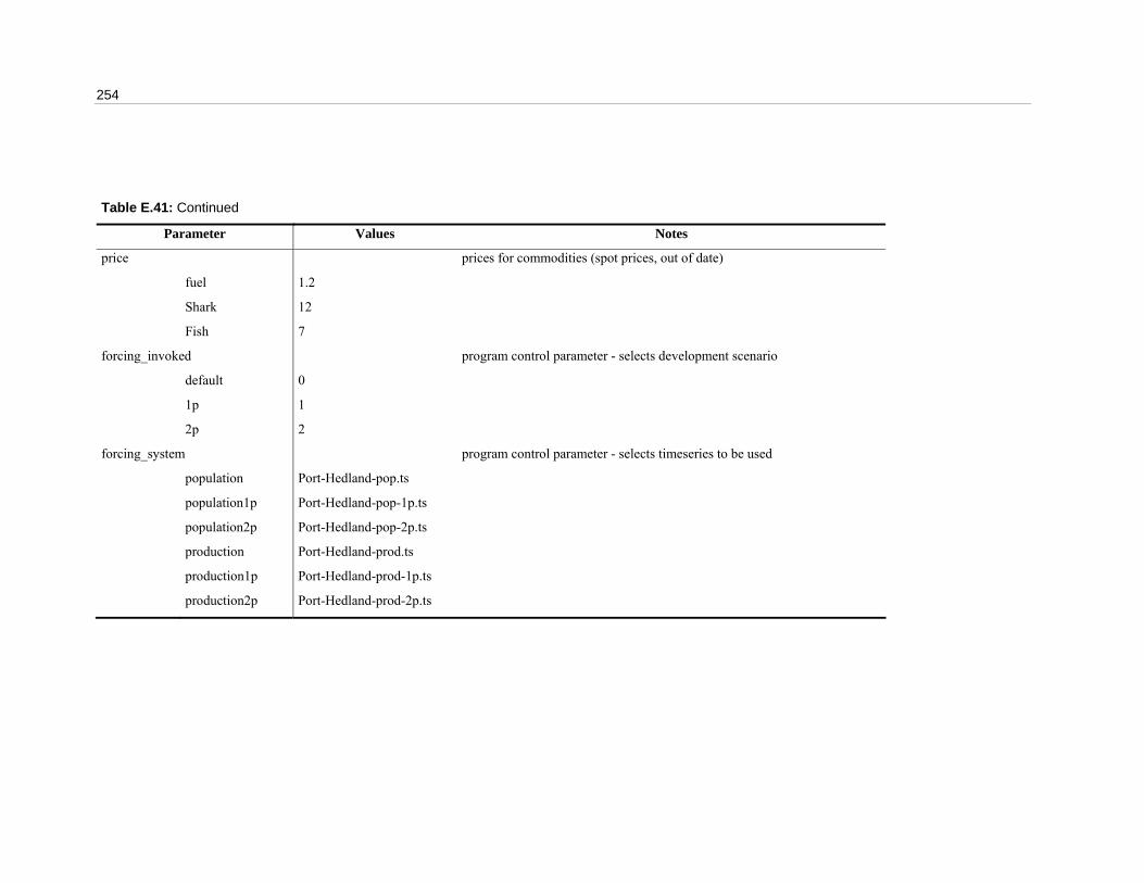
254
Table E.41: Continued
Parameter Values Notes
price prices for commodities (spot prices, out of date)
fuel 1.2
Shark 12
Fish 7
forcing_invoked program control parameter - selects development scenario
default 0
1p 1
2p 2
forcing_system program control parameter - selects timeseries to be used
population Port-Hedland-pop.ts
population1p Port-Hedland-pop-1p.ts
population2p Port-Hedland-pop-2p.ts
production Port-Hedland-prod.ts
production1p Port-Hedland-prod-1p.ts
production2p Port-Hedland-prod-2p.ts

Appendix E: InVitro agent files 255
Table E.42: US file - specifies destination for vessels.
Parameter Values Notes
name US
neighbours 20 determines max number of neighbours considered
capacity 1000
location
longitude 119
latitude -17.5
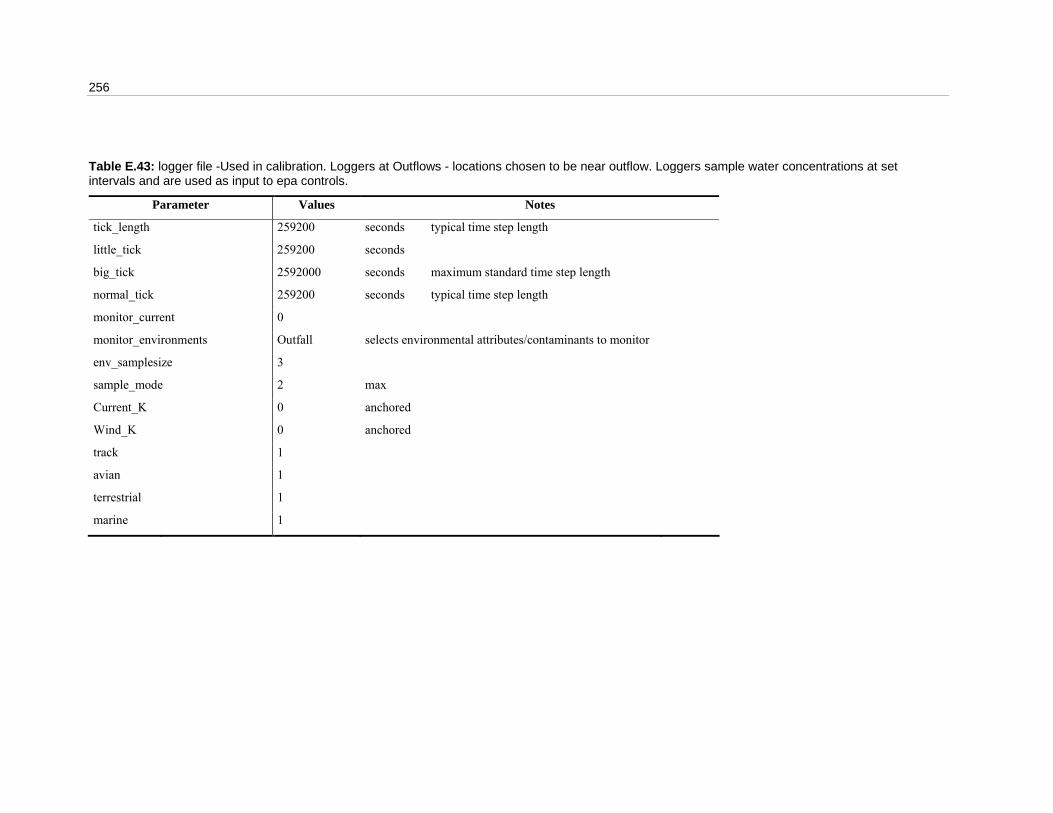
256
Table E.43: logger file -Used in calibration. Loggers at Outflows - locations chosen to be near outflow. Loggers sample water concentrations at set intervals and are used as input to epa controls.
Parameter Values Notes
tick_length 259200 seconds typical time step length
little_tick 259200 seconds
big_tick 2592000 seconds maximum standard time step length
normal_tick 259200 seconds typical time step length
monitor_current 0
monitor_environments Outfall selects environmental attributes/contaminants to monitor
env_samplesize 3
sample_mode 2 max
Current_K 0 anchored
Wind_K 0 anchored
track 1
avian 1
terrestrial 1
marine 1
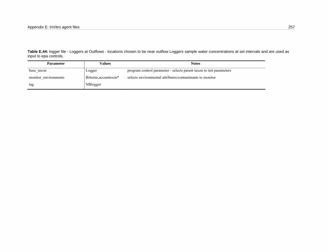
Appendix E: InVitro agent files 257
Table E.44: logger file - Loggers at Outflows - locations chosen to be near outflow Loggers sample water concentrations at set intervals and are used as input to epa controls.
Parameter Values Notes
base_taxon Logger program control parameter - selects parent taxon to init parameters
monitor_environments Bitterns,accumtoxin* selects environmental attributes/contaminants to monitor
tag NBlogger

258
Table E.45: dot file - Department of Transport.
Parameter Values Notes
Department of Transport - no parameters
name dot
tick_length 86400 seconds typical time step length

Appendix E: InVitro agent files 259
Table E.46: stdvessel file – parameters for standard shipping vessels.
Parameter Values Notes
tick_length 4800 seconds typical time step length
bored_tick 172800 seconds maximum standard time step length
alarmed_tick 1200 seconds standard time step length if in active state
neighbours 20 determines max number of neighbours considered
TimeInPort 21600 time between fishing excursions – assumes six hours to load/unload
SpeedInPort 0 limits vessel speed in port – must be zero while “in port”
speed 8
maxspeed 8
FuelCapacity 15000 adequate for duration of transits – need not be true value
FuelEfficiency 0.01 s-1 estimated from capacity and duration
VoyageLength 30 days
Percpetion_Range 20
ExclusionZone 50
min_depth -10 minimum ocean depth for vessels – adequate for a physical constraint in the model runs
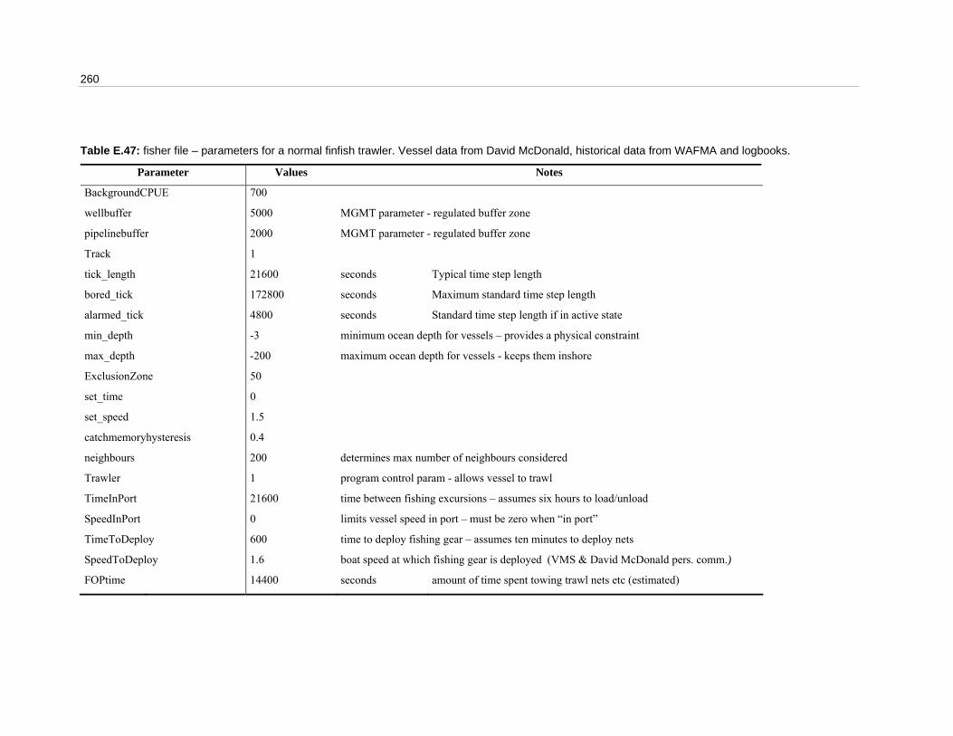
260
Table E.47: fisher file – parameters for a normal finfish trawler. Vessel data from David McDonald, historical data from WAFMA and logbooks.
Parameter Values Notes
BackgroundCPUE 700
wellbuffer 5000 MGMT parameter - regulated buffer zone
pipelinebuffer 2000 MGMT parameter - regulated buffer zone
Track 1
tick_length 21600 seconds Typical time step length
bored_tick 172800 seconds Maximum standard time step length
alarmed_tick 4800 seconds Standard time step length if in active state
min_depth -3 minimum ocean depth for vessels – provides a physical constraint
max_depth -200 maximum ocean depth for vessels - keeps them inshore
ExclusionZone 50
set_time 0
set_speed 1.5
catchmemoryhysteresis 0.4
neighbours 200 determines max number of neighbours considered
Trawler 1 program control param - allows vessel to trawl
TimeInPort 21600 time between fishing excursions – assumes six hours to load/unload
SpeedInPort 0 limits vessel speed in port – must be zero when “in port”
TimeToDeploy 600 time to deploy fishing gear – assumes ten minutes to deploy nets
SpeedToDeploy 1.6 boat speed at which fishing gear is deployed (VMS & David McDonald pers. comm.)
FOPtime 14400 seconds amount of time spent towing trawl nets etc (estimated)

Appendix E: InVitro agent files 261
Table E.47: Continued
Parameter Values Notes
FOPspeed 1.75 boat speed at which the nets are towed (VMS & David McDonald pers. comm.)
HaulingTime 1200 How long it takes to haul the gear in – assumed to be twenty minutes
HaulingSpeed 1.6 boat speed at which the gear are hauled -- assumed to be the same as deployment
ProcessingTime 1800 time it takes to stow fish – taken to be half an hour
ProcessingSpeed 0 vessel speed which processing – ship is taken to be stationary during processing
speed 3
maxspeed 4
HoldCapacity 4500 Consensus value (David McDonald pers. comm.m.)
FuelCapacity 40000 Consensus value (David McDonald pers. comm.m.)
FuelPrice 1
vmsEffortRatio 0.68
FuelEfficiency 0.01 s-1 estimated from capacity and duration
Mesh 0.12 Somewhere between 4 & 4.5 inches net mesh (consensus value, David McDonald pers. comm.)
Efficiency efficiency of gear – Not used on Populations
default 0.1
HighEfficiency 0.5
BenthicEfficiency 0.05 Landing efficiency of gear (Hall 2000)
HookCount 0
VoyageLength 14 days
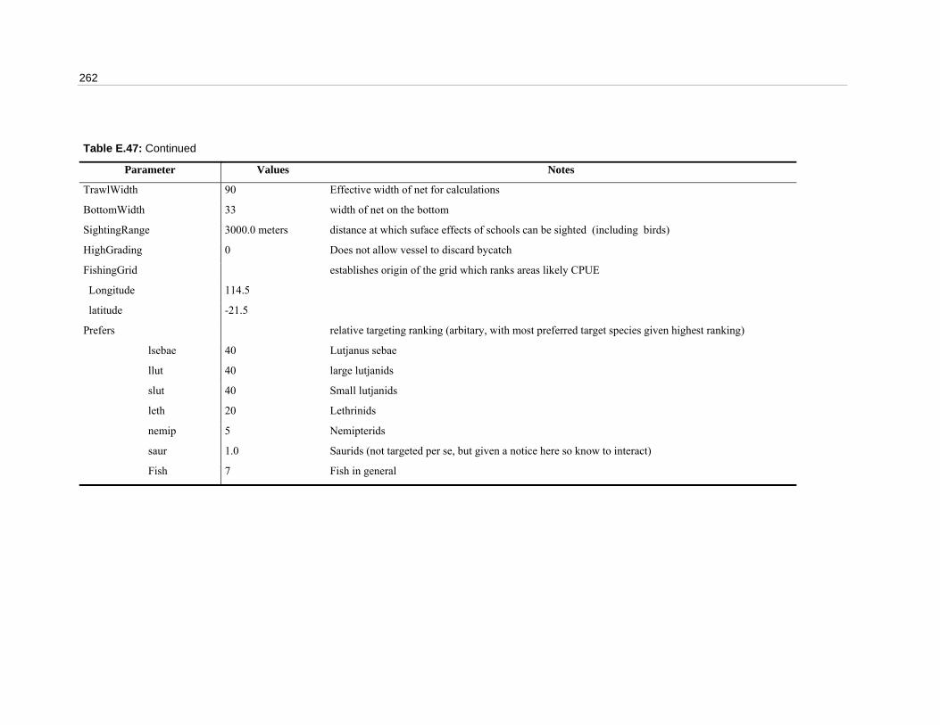
262
Table E.47: Continued
Parameter Values Notes
TrawlWidth 90 Effective width of net for calculations
BottomWidth 33 width of net on the bottom
SightingRange 3000.0 meters distance at which suface effects of schools can be sighted (including birds)
HighGrading 0 Does not allow vessel to discard bycatch
FishingGrid establishes origin of the grid which ranks areas likely CPUE
Longitude 114.5
latitude -21.5
Prefers relative targeting ranking (arbitary, with most preferred target species given highest ranking)
lsebae 40 Lutjanus sebae
llut 40 large lutjanids
slut 40 Small lutjanids
leth 20 Lethrinids
nemip 5 Nemipterids
saur 1.0 Saurids (not targeted per se, but given a notice here so know to interact)
Fish 7 Fish in general
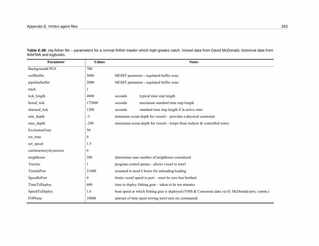
Appendix E: InVitro agent files 263
Table E.48: ntq-fisher file – parameters for a normal finfish trawler which high-grades catch. Vessel data from David McDonald, historical data from WAFMA and logbooks.
Parameter Values Notes
BackgroundCPUE 700
wellbuffer 5000 MGMT parameter - regulated buffer zone
pipelinebuffer 2000 MGMT parameter - regulated buffer zone
track 1
tick_length 4800 seconds typical time step length
bored_tick 172800 seconds maximum standard time step length
alarmed_tick 1200 seconds standard time step length if in active state
min_depth -3 minimum ocean depth for vessels – provides a physical constraint
max_depth -200 maximum ocean depth for vessels - keeps them inshore & controlled zones
ExclusionZone 50
set_time 0
set_speed 1.5
catchmemoryhysteresis 0
neighbours 200 determines max number of neighbours considered
Trawler 1 program control param - allows vessel to trawl
TimeInPort 21600 assumed to need 6 hours for unloading/loading
SpeedInPort 0 limits vessel speed in port – must be zero hen berthed
TimeToDeploy 600 time to deploy fishing gear – taken to be ten minutes
SpeedToDeploy 1.6 boat speed at which fishing gear is deployed (VMS & Consensus data via D. McDonald pers. comm.)
FOPtime 10800 amount of time spent towing trawl nets etc (estimated)
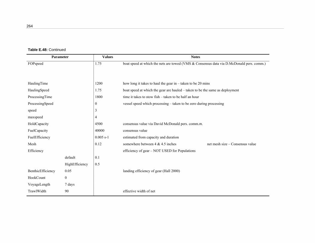
264
Table E.48: Continued
Parameter Values Notes
FOPspeed 1.75 boat speed at which the nets are towed (VMS & Consensus data via D.McDonald pers. comm.)
HaulingTime 1200 how long it takes to haul the gear in – taken to be 20 mins
HaulingSpeed 1.75 boat speed at which the gear are hauled – taken to be the same as deployment
ProcessingTime 1800 time it takes to stow fish – taken to be half an hour
ProcessingSpeed 0 vessel speed which processing – taken to be zero during processing
speed 3
maxspeed 4
HoldCapacity 4500 consensus value via David McDonald pers. comm.m.
FuelCapacity 40000 consensus value
FuelEfficiency 0.005 s-1 estimated from capacity and duration
Mesh 0.12 somewhere between 4 & 4.5 inches net mesh size – Consensus value
Efficiency efficiency of gear – NOT USED for Populations
default 0.1
HighEfficiency 0.5
BenthicEfficiency 0.05 landing efficiency of gear (Hall 2000)
HookCount 0
VoyageLength 7 days
TrawlWidth 90 effective width of net
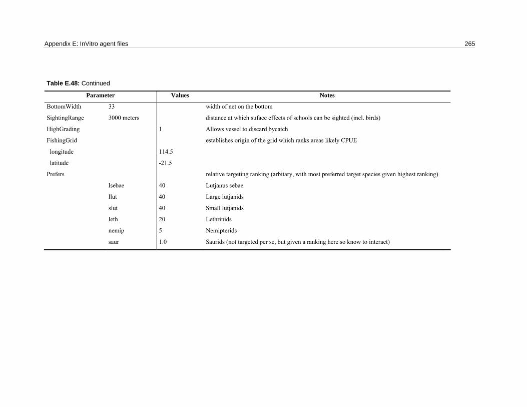
Appendix E: InVitro agent files 265
Table E.48: Continued
Parameter Values Notes
BottomWidth 33 width of net on the bottom
SightingRange 3000 meters distance at which suface effects of schools can be sighted (incl. birds)
HighGrading 1 Allows vessel to discard bycatch
FishingGrid establishes origin of the grid which ranks areas likely CPUE
longitude 114.5
latitude -21.5
Prefers relative targeting ranking (arbitary, with most preferred target species given highest ranking)
lsebae 40 Lutjanus sebae
llut 40 Large lutjanids
slut 40 Small lutjanids
leth 20 Lethrinids
nemip 5 Nemipterids
saur 1.0 Saurids (not targeted per se, but given a ranking here so know to interact)
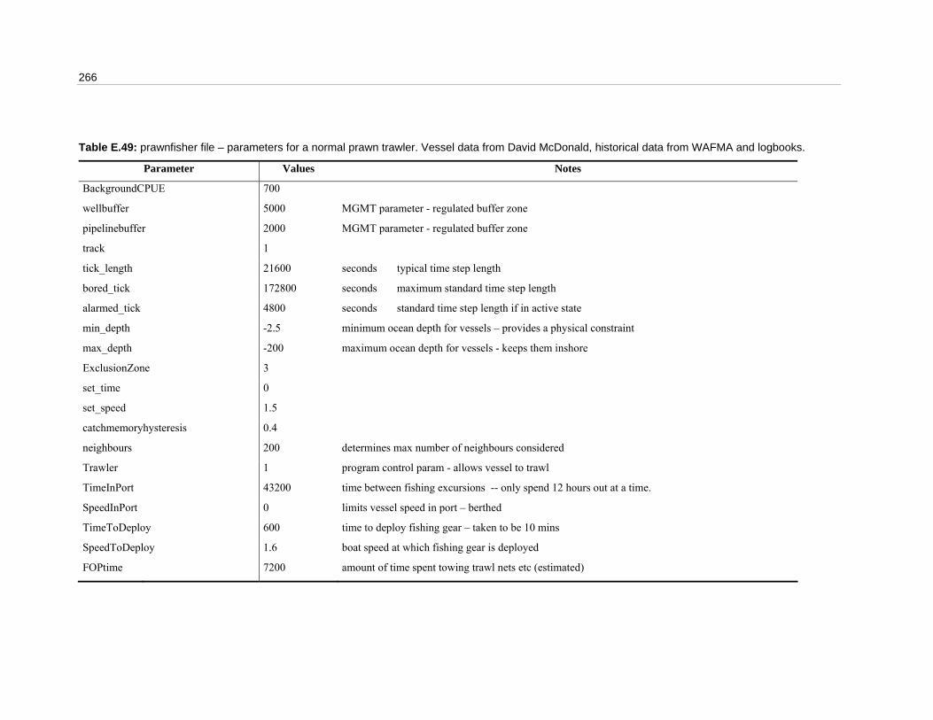
266
Table E.49: prawnfisher file – parameters for a normal prawn trawler. Vessel data from David McDonald, historical data from WAFMA and logbooks.
Parameter Values Notes
BackgroundCPUE 700
wellbuffer 5000 MGMT parameter - regulated buffer zone
pipelinebuffer 2000 MGMT parameter - regulated buffer zone
track 1
tick_length 21600 seconds typical time step length
bored_tick 172800 seconds maximum standard time step length
alarmed_tick 4800 seconds standard time step length if in active state
min_depth -2.5 minimum ocean depth for vessels – provides a physical constraint
max_depth -200 maximum ocean depth for vessels - keeps them inshore
ExclusionZone 3
set_time 0
set_speed 1.5
catchmemoryhysteresis 0.4
neighbours 200 determines max number of neighbours considered
Trawler 1 program control param - allows vessel to trawl
TimeInPort 43200 time between fishing excursions -- only spend 12 hours out at a time.
SpeedInPort 0 limits vessel speed in port – berthed
TimeToDeploy 600 time to deploy fishing gear – taken to be 10 mins
SpeedToDeploy 1.6 boat speed at which fishing gear is deployed
FOPtime 7200 amount of time spent towing trawl nets etc (estimated)

Appendix E: InVitro agent files 267
Table E.49: Continued
Parameter Values Notes
FOPspeed 1.75 boat speed at which the nets are towed
HaulingTime 1200 how long it takes to haul the gear in – taken to be 20 mins
HaulingSpeed 1.6 boat speed at which the gear is hauled in
ProcessingTime 1800 time it takes to stow fish – taken to be half an hour
ProcessingSpeed 0 vessel speed which processing – boat is taken to be stationary during sorting
speed 3
maxspeed 4
HoldCapacity 4500 taken to be the same as the finfish
FuelCapacity 40000 taken to be the same as the finfish – not critical, since the prawn trawlers have shorter trips
FuelEfficiency 0.05 s-1 estimated from capacity and duration
Mesh 0.01 it is *really* 2cm, but the prawns manage to get through :-(
Efficiency landing efficiency of gear
Default 0.1
HighEfficiency 0.5
BenthicEfficiency 0.1 landing efficiency of gear
HookCount 0
VoyageLength 7 days
TrawlWidth 90 effective width of net
BottomWidth 33 width of net on the bottom
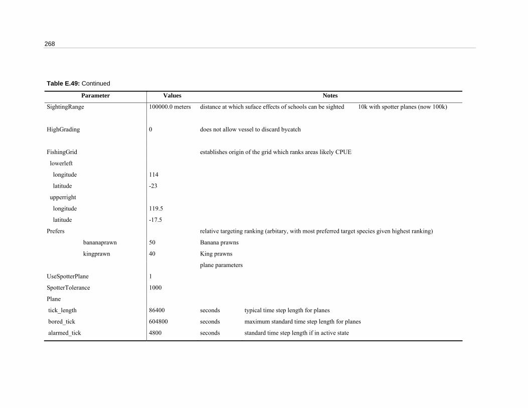
268
Table E.49: Continued
Parameter Values Notes
SightingRange 100000.0 meters distance at which suface effects of schools can be sighted 10k with spotter planes (now 100k)
HighGrading 0 does not allow vessel to discard bycatch
FishingGrid establishes origin of the grid which ranks areas likely CPUE
lowerleft
longitude 114
latitude -23
upperright
longitude 119.5
latitude -17.5
Prefers relative targeting ranking (arbitary, with most preferred target species given highest ranking)
bananaprawn 50 Banana prawns
kingprawn 40 King prawns
plane parameters
UseSpotterPlane 1
SpotterTolerance 1000
Plane
tick_length 86400 seconds typical time step length for planes
bored_tick 604800 seconds maximum standard time step length for planes
alarmed_tick 4800 seconds standard time step length if in active state

Appendix E: InVitro agent files 269
Table E.50: fishing_survey file – parameters for a normal stock survey trawler.
Parameter Values Notes
BackgroundCPUE 700
wellbuffer 5000 MGMT parameter - regulated buffer zone
pipelinebuffer 2000 MGMT parameter - regulated buffer zone
track 1
tick_length 4800 seconds typical time step length
bored_tick 172800 seconds maximum standard time step length
alarmed_tick 1200 seconds standard time step length if in active state
min_depth -3 minimum ocean depth for vessels -- provides physical constraint
max_depth -200 maximum ocean depth for vessels - keeps them inshore
ExclusionZone 50
set_time 0
set_speed 1.5
CatchMemoryHysteresis 0.4
neighbours 200 determines max number of neighbours considered
Trawler 1 program control param - allows vessel to trawl
TimeInPort 21600 time between fishing excursions – load/unload
SpeedInPort 0 limits vessel speed in port – berthed
TimeToDeploy 600 time to deploy fishing gear – taken to be ten minutes
SpeedToDeploy 1.6 boat speed at which fishing gear is deployed – same as for finfish trawl
FOPtime 10800 amount of time spent towing trawl nets etc (estimated in finfish trawl)
FOPspeed 1.75 boat speed at which the nets are towed – same as finfish trawl
HaulingTime 1200 how long it takes to haul the gear in -- taken to be 20 minutes, as for commercial trawl
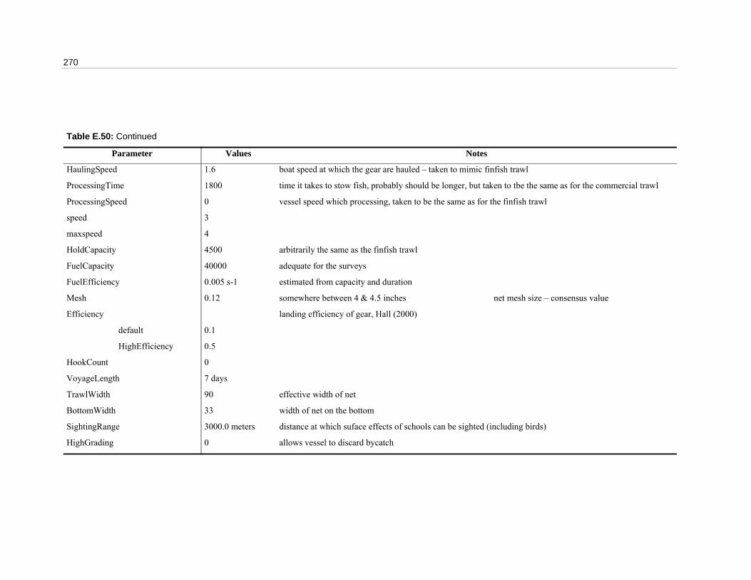
270
Table E.50: Continued
Parameter Values Notes
HaulingSpeed 1.6 boat speed at which the gear are hauled – taken to mimic finfish trawl
ProcessingTime 1800 time it takes to stow fish, probably should be longer, but taken to tbe the same as for the commercial trawl
ProcessingSpeed 0 vessel speed which processing, taken to be the same as for the finfish trawl
speed 3
maxspeed 4
HoldCapacity 4500 arbitrarily the same as the finfish trawl
FuelCapacity 40000 adequate for the surveys
FuelEfficiency 0.005 s-1 estimated from capacity and duration
Mesh 0.12 somewhere between 4 & 4.5 inches net mesh size – consensus value
Efficiency landing efficiency of gear, Hall (2000)
default 0.1
HighEfficiency 0.5
HookCount 0
VoyageLength 7 days
TrawlWidth 90 effective width of net
BottomWidth 33 width of net on the bottom
SightingRange 3000.0 meters distance at which suface effects of schools can be sighted (including birds)
HighGrading 0 allows vessel to discard bycatch
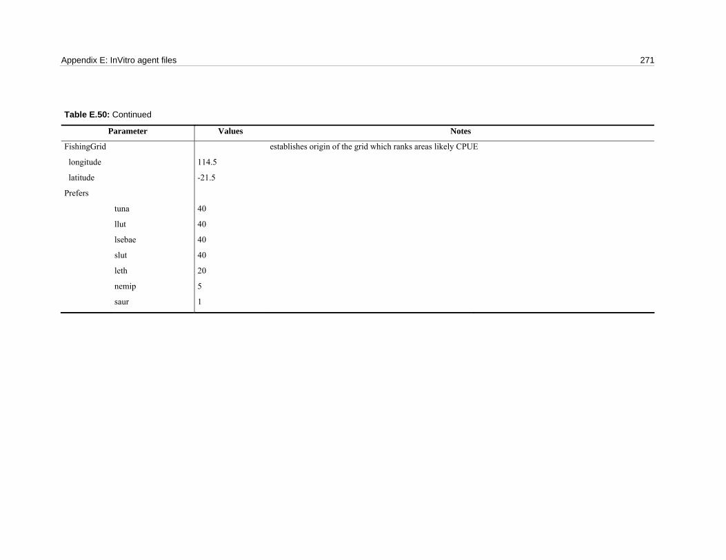
Appendix E: InVitro agent files 271
Table E.50: Continued
Parameter Values Notes
FishingGrid establishes origin of the grid which ranks areas likely CPUE
longitude 114.5
latitude -21.5
Prefers
tuna 40
llut 40
lsebae 40
slut 40
leth 20
nemip 5
saur 1

272
Table E.51: trap-fisher file – parameters for a normal trap fishing vessels. Vessel data from David McDonald, historical data from WAFMA and logbooks.
Parameter Values Notes
BackgroundCPUE 700
wellbuffer 500 MGMT parameter - regulated buffer zone
pipelinebuffer 500 MGMT parameter - regulated buffer zone
MaximumFishingDepth -200
track 1
tick_length 4800 seconds typical time step length
bored_tick 172800 seconds maximum standard time step length
alarmed_tick 1200 seconds standard time step length if in active state
min_depth -3 minimum ocean depth for vessels – establishes physical constraint
max_depth -200 maximum ocean depth for vessels - keeps them inshore
ExclusionZone 50
set_time 0
set_speed 1.5
catchmemoryhysteresis 0.4
neighbours 20 dtermines max number of neighbours considered
#Trawler 1 program control param - defaults to zero: does not allow vessel to trawl
Trapper 1 program control param - allows vessel to set traps
TimeInPort 21600 time between fishing excursions – taken to be 6 hours
SpeedInPort 0 limits vessel speed in port – berthed
TimeToDeploy 600 time to deploy fishing gear – taken to be ten minutes
SpeedToDeploy 0 boat speed at which fishing gear is deployed – boat stops to deploy traps
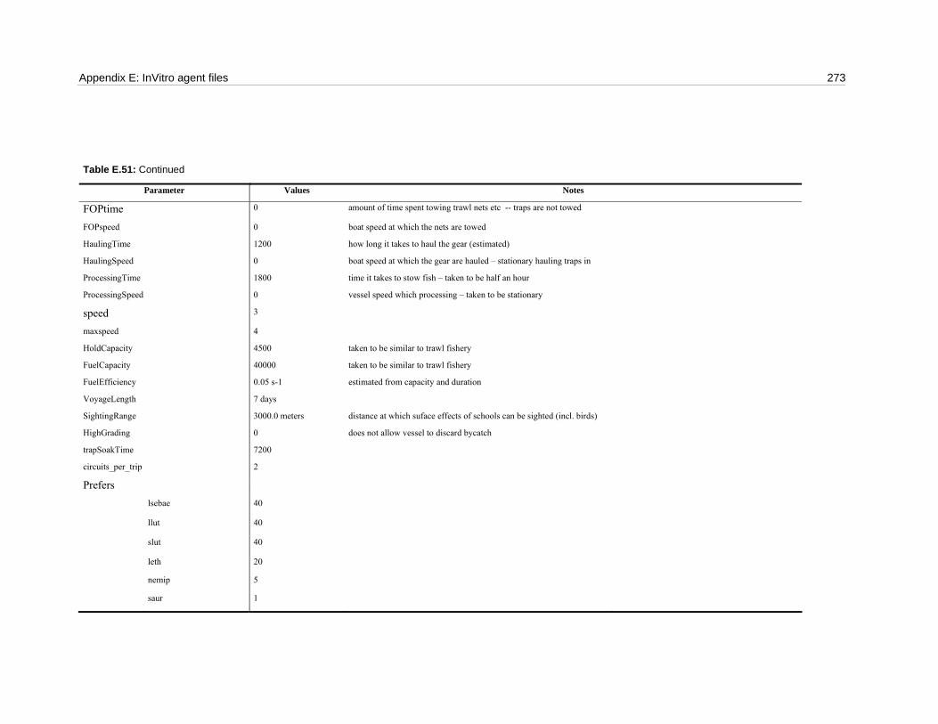
Appendix E: InVitro agent files 273
Table E.51: Continued
Parameter Values Notes
FOPtime 0 amount of time spent towing trawl nets etc -- traps are not towed
FOPspeed 0 boat speed at which the nets are towed
HaulingTime 1200 how long it takes to haul the gear (estimated)
HaulingSpeed 0 boat speed at which the gear are hauled – stationary hauling traps in
ProcessingTime 1800 time it takes to stow fish – taken to be half an hour
ProcessingSpeed 0 vessel speed which processing – taken to be stationary
speed 3
maxspeed 4
HoldCapacity 4500 taken to be similar to trawl fishery
FuelCapacity 40000 taken to be similar to trawl fishery
FuelEfficiency 0.05 s-1 estimated from capacity and duration
VoyageLength 7 days
SightingRange 3000.0 meters distance at which suface effects of schools can be sighted (incl. birds)
HighGrading 0 does not allow vessel to discard bycatch
trapSoakTime 7200
circuits_per_trip 2
Prefers
lsebae 40
llut 40
slut 40
leth 20
nemip 5
saur 1
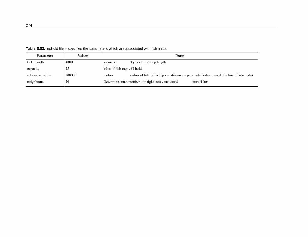
274
Table E.52: leghold file – specifies the parameters which are associated with fish traps.
Parameter Values Notes
tick_length 4800 seconds Typical time step length
capacity 25 kilos of fish trap will hold
influence_radius 100000 metres radius of total effect (population-scale parameterisation; would be fine if fish-scale)
neighbours 20 Determines max number of neighbours considered from fisher

Appendix E: InVitro agent files 275
Table E.53: fishWAFMA file – Management Authority for the prawn fisheries.
Parameter Values Notes
global_callback program control parameter
integrated-management 1 program control parameter - controls mgmt mode
default 0

276
Table E.54: popWAFMA file – Management Authority for the finfish fisheries.
Parameter Values Notes
global_callback program control parameter
integrated-management 1 program control parameter - controls mgmt mode
default 0

Appendix E: InVitro agent files 277
Table E.55: popBiomass file – specifies the periodicity of the population reporting from within the model. PopBiomass also applies historical mortality.
Parameter Values Notes
schedule @01/15

278
Table E.56: popage file – specifies when the juvenile finfish populations are recruited to the adult population (program parameter).
Parameter Values Notes
schedule @12/15

Appendix E: InVitro agent files 279
Table E.57: sharkesky file – sets parameters for tracking shark biomass and triggering management actions in scenarios with integrated management.
Parameter Values Notes
global_callback program control parameter
integrated-management 1 program control parameter - controls mgmt mode
default 0
epa_trigger
numbers -1 take the value from the end of the historical period
biomass 0 don't use biomass
mean_mass 0 or mean_mass
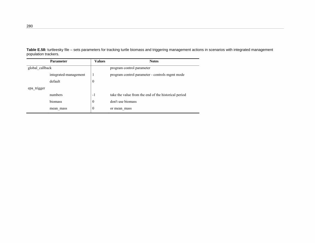
280
Table E.58: turtleesky file – sets parameters for tracking turtle biomass and triggering management actions in scenarios with integrated management population trackers.
Parameter Values Notes
global_callback program control parameter
integrated-management 1 program control parameter - controls mgmt mode
default 0
epa_trigger
numbers -1 take the value from the end of the historical period
biomass 0 don't use biomass
mean_mass 0 or mean_mass

Appendix F: InVitro configuration files 281
APPENDIX F: INVITRO CONFIGURATION FILES
These tables contain the configuration files used in the NWSJEMS MSE runs. The format for these files is:
<agent type> <taxon or agent name> <start time> <end time> <configuration parameters>
A start or end time of 0 indicates that the agent will commence (or end) with the entire simulation rather than on a specific date.
The configuration parameters typically include the latitude and longitude of their starting position or extent, whether they are to be tracked, their periodicity of output and a sting list of other agent types they may be interested in.
Class Name Start End Location in Model Space Size Proj
DB Projection Cell No Suppress
Output Period Sm. scale
Report period Lg. scale
Report period Report file Targets
Adviser adv1: 0 0 -720643 -2.20E+06 -619999 -2.08E+06 0.1 map.rc none 1 0 quarterly quarterly Yearly adv1.mon.pt Mangroves Seagrass llut lsebae Slut nemip leth saur Sponge kingprawn bananaprawn shark turtle oysterlease
Adviser adv2: 0 0 -720643 -2.08E+06 -619999 -1.97E+06 0.1 map.rc none 2 0 quarterly quarterly yearly adv2.mon.pt Mangroves Seagrass llut lsebae Slut nemip leth saur Sponge kingprawn bananaprawn shark turtle oysterlease
Adviser adv3: 0 0 -720643 -1.97E+06 -619999 -1.85E+06 0.1 map.rc none 3 0 quarterly quarterly yearly adv3.mon.pt Mangroves Seagrass llut lsebae Slut nemip leth saur Sponge kingprawn bananaprawn shark turtle oysterlease
Adviser adv4: 0 0 -720643 -1.85E+06 -619999 -1.74E+06 0.1 map.rc none 4 0 quarterly quarterly yearly adv4.mon.pt Mangroves Seagrass llut lsebae Slut nemip leth saur Sponge kingprawn bananaprawn shark turtle oysterlease

282
Class Name Start End Location in Model Space Size Proj DB
Projection Cell No Suppress Output
Period Sm. scale Report period
Lg. scale Report period
Report file Targets
Adviser adv5: 0 0 -720643 -1.74E+06 -619999 -1.63E+06 0.1 map.rc none 5 0 quarterly quarterly yearly adv5.mon.pt Mangroves Seagrass llut lsebae Slut nemip leth saur Sponge kingprawn bananaprawn shark turtle oysterlease
Adviser adv6: 0 0 -619999 -2.20E+06 -519355 -2.08E+06 0.1 map.rc none 6 0 quarterly quarterly yearly adv6.mon.pt Mangroves Seagrass llut lsebae Slut nemip leth saur Sponge kingprawn bananaprawn shark turtle oysterlease
Adviser adv7: 0 0 -619999 -2.08E+06 -519355 -1.97E+06 0.1 map.rc none 7 0 quarterly quarterly yearly adv7.mon.pt Mangroves Seagrass llut lsebae Slut nemip leth saur Sponge kingprawn bananaprawn shark turtle oysterlease
Adviser adv8: 0 0 -619999 -1.97E+06 -519355 -1.85E+06 0.1 map.rc none 8 0 quarterly quarterly yearly adv8.mon.pt Mangroves Seagrass llut lsebae Slut nemip leth saur Sponge kingprawn bananaprawn shark turtle oysterlease
Adviser adv9: 0 0 -619999 -1.85E+06 -519355 -1.74E+06 0.1 map.rc none 9 0 quarterly quarterly yearly adv9.mon.pt Mangroves Seagrass llut lsebae Slut nemip leth saur Sponge kingprawn bananaprawn shark turtle oysterlease
Adviser adv10: 0 0 -619999 -1.74E+06 -519355 -1.63E+06 0.1 map.rc none 10 0 quarterly quarterly yearly adv10.mon.pt Mangroves Seagrass llut lsebae Slut nemip leth saur Sponge kingprawn bananaprawn shark turtle oysterlease
Adviser adv11: 0 0 -519355 -2.08E+06 -418711 -1.97E+06 0.1 map.rc none 11 0 quarterly quarterly yearly adv11.mon.pt Mangroves Seagrass llut lsebae Slut nemip leth saur Sponge kingprawn bananaprawn shark turtle oysterlease

Appendix F: InVitro configuration files 283
Class Name Start End Location in Model Space Size Proj DB
Projection Cell No Suppress Output
Period Sm. scale Report period
Lg. scale Report period
Report file Targets
Adviser adv12: 0 0 -519355 -1.97E+06 -418711 -1.85E+06 0.1 map.rc none 12 0 quarterly quarterly yearly adv12.mon.pt Mangroves Seagrass llut lsebae Slut nemip leth saur Sponge kingprawn bananaprawn shark turtle oysterlease
Adviser adv13: 0 0 -519355 -1.85E+06 -418711 -1.74E+06 0.1 map.rc none 13 0 quarterly quarterly yearly adv13.mon.pt Mangroves Seagrass llut lsebae Slut nemip leth saur Sponge kingprawn bananaprawn shark turtle oysterlease
Adviser adv14: 0 0 -519355 -1.74E+06 -418711 -1.63E+06 0.1 map.rc none 14 0 quarterly quarterly yearly adv14.mon.pt Mangroves Seagrass llut lsebae Slut nemip leth saur Sponge kingprawn bananaprawn shark turtle oysterlease
Adviser adv15: 0 0 -418711 -2.08E+06 -318067 -1.97E+06 0.1 map.rc none 15 0 quarterly quarterly yearly adv15.mon.pt Mangroves Seagrass llut lsebae Slut nemip leth saur Sponge kingprawn bananaprawn shark turtle oysterlease
Adviser adv16: 0 0 -418711 -1.97E+06 -318067 -1.85E+06 0.1 map.rc none 16 0 quarterly quarterly yearly adv16.mon.pt Mangroves Seagrass llut lsebae Slut nemip leth saur Sponge kingprawn bananaprawn shark turtle oysterlease
Adviser adv17: 0 0 -418711 -1.85E+06 -318067 -1.74E+06 0.1 map.rc none 17 0 quarterly quarterly yearly adv17.mon.pt Mangroves Seagrass llut lsebae Slut nemip leth saur Sponge kingprawn bananaprawn shark turtle oysterlease
Adviser adv18: 0 0 -418711 -1.74E+06 -318067 -1.63E+06 0.1 map.rc none 18 0 quarterly quarterly yearly adv18.mon.pt Mangroves Seagrass llut lsebae Slut nemip leth saur Sponge kingprawn bananaprawn shark turtle oysterlease
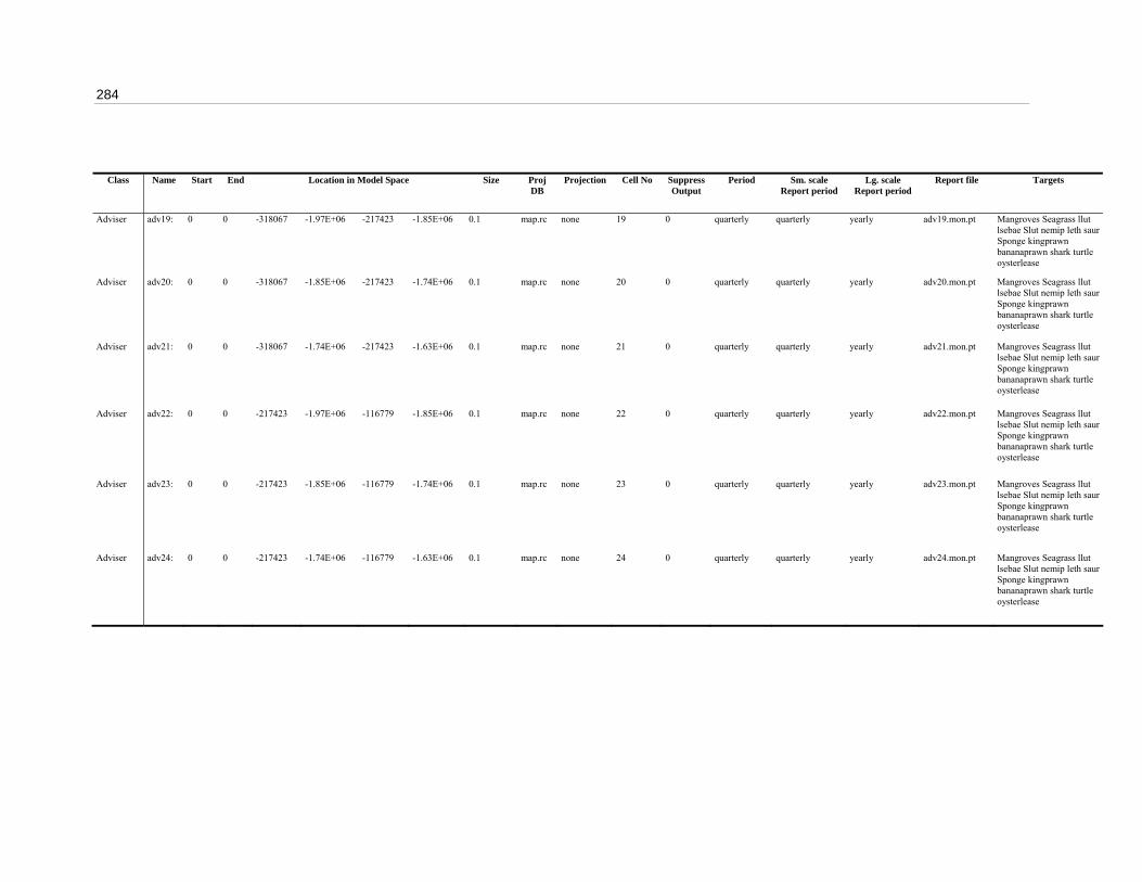
284
Class Name Start End Location in Model Space Size Proj DB
Projection Cell No Suppress Output
Period Sm. scale Report period
Lg. scale Report period
Report file Targets
Adviser adv19: 0 0 -318067 -1.97E+06 -217423 -1.85E+06 0.1 map.rc none 19 0 quarterly quarterly yearly adv19.mon.pt Mangroves Seagrass llut lsebae Slut nemip leth saur Sponge kingprawn bananaprawn shark turtle oysterlease
Adviser adv20: 0 0 -318067 -1.85E+06 -217423 -1.74E+06 0.1 map.rc none 20 0 quarterly quarterly yearly adv20.mon.pt Mangroves Seagrass llut lsebae Slut nemip leth saur Sponge kingprawn bananaprawn shark turtle oysterlease
Adviser adv21: 0 0 -318067 -1.74E+06 -217423 -1.63E+06 0.1 map.rc none 21 0 quarterly quarterly yearly adv21.mon.pt Mangroves Seagrass llut lsebae Slut nemip leth saur Sponge kingprawn bananaprawn shark turtle oysterlease
Adviser adv22: 0 0 -217423 -1.97E+06 -116779 -1.85E+06 0.1 map.rc none 22 0 quarterly quarterly yearly adv22.mon.pt Mangroves Seagrass llut lsebae Slut nemip leth saur Sponge kingprawn bananaprawn shark turtle oysterlease
Adviser adv23: 0 0 -217423 -1.85E+06 -116779 -1.74E+06 0.1 map.rc none 23 0 quarterly quarterly yearly adv23.mon.pt Mangroves Seagrass llut lsebae Slut nemip leth saur Sponge kingprawn bananaprawn shark turtle oysterlease
Adviser adv24: 0 0 -217423 -1.74E+06 -116779 -1.63E+06 0.1 map.rc none 24 0 quarterly quarterly yearly adv24.mon.pt Mangroves Seagrass llut lsebae Slut nemip leth saur Sponge kingprawn bananaprawn shark turtle oysterlease
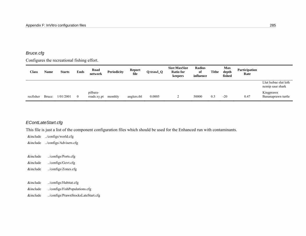
Appendix F: InVitro configuration files 285
Bruce.cfg Configures the recreational fishing effort.
Class Name Starts Ends Road network Periodicity Report
file Q:trawl_Q Size:MaxSize
Ratio for keepers
Radius of
influence Tithe
Max depthfished
Participation Rate
recfisher Bruce: 1/01/2001 0 pilbara-roads.xy.pt monthly anglers.tbl 0.0005 2 50000 0.3 -20 0.47
Llut lsebae slut leth nemip saur shark
Kingprawn Bananaprawn turtle
EContLateStart.cfg This file is just a list of the component configuration files which should be used for the Enhanced run with contaminants. &include ../configs/world.cfg
&include ../configs/Advisers.cfg
&include ../configs/Ports.cfg
&include ../configs/Govt.cfg
&include ../configs/Zones.cfg
&include ../configs/Habitat.cfg
&include ../configs/FishPopulations.cfg
&include ../configs/PrawnStocksLateStart.cfg
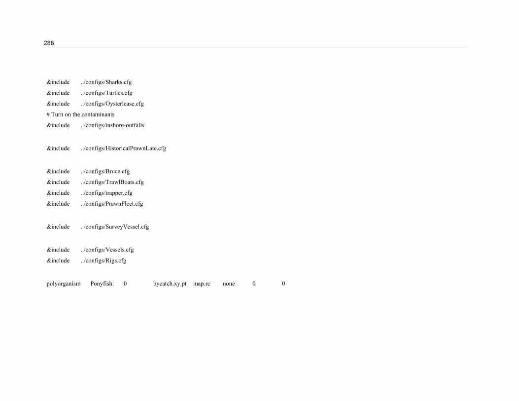
286
&include ../configs/Sharks.cfg
&include ../configs/Turtles.cfg
&include ../configs/Oysterlease.cfg
# Turn on the contaminants
&include ../configs/inshore-outfalls
&include ../configs/HistoricalPrawnLate.cfg
&include ../configs/Bruce.cfg
&include ../configs/TrawlBoats.cfg
&include ../configs/trapper.cfg
&include ../configs/PrawnFleet.cfg
&include ../configs/SurveyVessel.cfg
&include ../configs/Vessels.cfg
&include ../configs/Rigs.cfg
polyorganism Ponyfish: 0 bycatch.xy.pt map.rc none 0 0

Appendix F: InVitro configuration files 287
EContLateStart2p.cfg This file is just a list of the component configuration files which should be used for the Enhanced run with contaminants and the two pulse development.
&include ../configs/world.cfg
&include ../configs/Advisers.cfg
&include ../configs/Ports.cfg
&include ../configs/Govt.cfg
&include ../configs/Zones.cfg
&include ../configs/Habitat.cfg
&include ../configs/FishPopulations.cfg
&include ../configs/PrawnStocksLateStart.cfg
&include ../configs/Sharks.cfg
&include ../configs/Turtles.cfg
&include ../configs/Oysterlease.cfg
# Turn on the contaminants
&include ../configs/inshore-outfalls
&include ../configs/HistoricalPrawnLate.cfg
&include ../configs/Bruce.cfg
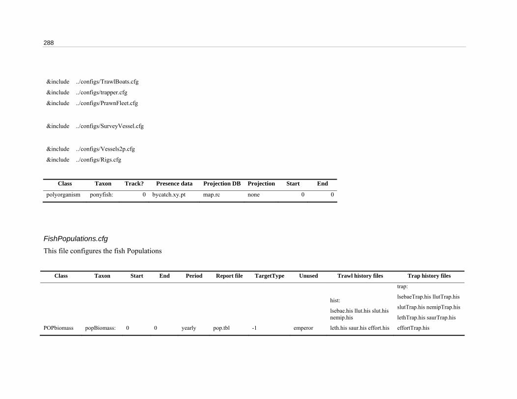
288
&include ../configs/TrawlBoats.cfg
&include ../configs/trapper.cfg
&include ../configs/PrawnFleet.cfg
&include ../configs/SurveyVessel.cfg
&include ../configs/Vessels2p.cfg
&include ../configs/Rigs.cfg
Class Taxon Track? Presence data Projection DB Projection Start End
polyorganism ponyfish: 0 bycatch.xy.pt map.rc none 0 0
FishPopulations.cfg This file configures the fish Populations
Class Taxon Start End Period Report file TargetType Unused Trawl history files Trap history files
POPbiomass popBiomass: 0 0 yearly pop.tbl -1 emperor
hist:
lsebae.his llut.his slut.his nemip.his
leth.his saur.his effort.his
trap:
lsebaeTrap.his llutTrap.his
slutTrap.his nemipTrap.his
lethTrap.his saurTrap.his
effortTrap.his

Appendix F: InVitro configuration files 289
Class Taxon Start End Period Targets
GraduatePop popage: 0 0 yearly Llut slut nemip saur leth lsebae
&include ../configs/LlutPopulations.cfg
&include ../configs/LethPopulations.cfg
&include ../configs/LsebaePopulations.cfg
&include ../configs/SlutPopulations.cfg
&include ../configs/SaurPopulations.cfg
&include ../configs/NemipPopulations.cfg
Govt.cfg Specifies “infrastructure” with an impact on the system
Class Taxon Start End Report file Input file Targets
catastrophe sandpit: 0 0 Dredged.dat Dredge.data Benthic animal

290
Habitat.cfg This file configures the benthic habitat agents and Monitors which track their state.
Class Taxon Track? Presence data Projection DB Projection Start End
benthic mangroves: 0 mangrovegrids.ll.pt map.rc nws 0 0
benthic seagrass: 0 macrophytegrids.ll.pt map.rc nws 0 0
benthic sponge: 0 porifera_grown.ll.pt map.rc nws 0 0
Class Taxon Start End Period Report file Target
tracker shoreplants: 3/01/1970 0 Yearly mangroves mangroves
tracker benthicplants: 3/01/1970 0 Yearly seagrass seagrass
tracker poriferas: 3/01/1970 0 Yearly sponge sponge
HistoricalPrawn.cfg Configures the agent which applies historical effort to prawn fishery.
Class Taxon Start End Period Report file Target type Unused Targets
FishBiomass fishBiomass: 0 0 monthly fishpop.tbl -1 emperor hist: KingPrawnSpatialCatch.his BananaPrawnSpatialCatch.his PrawnEffortSpatial.his
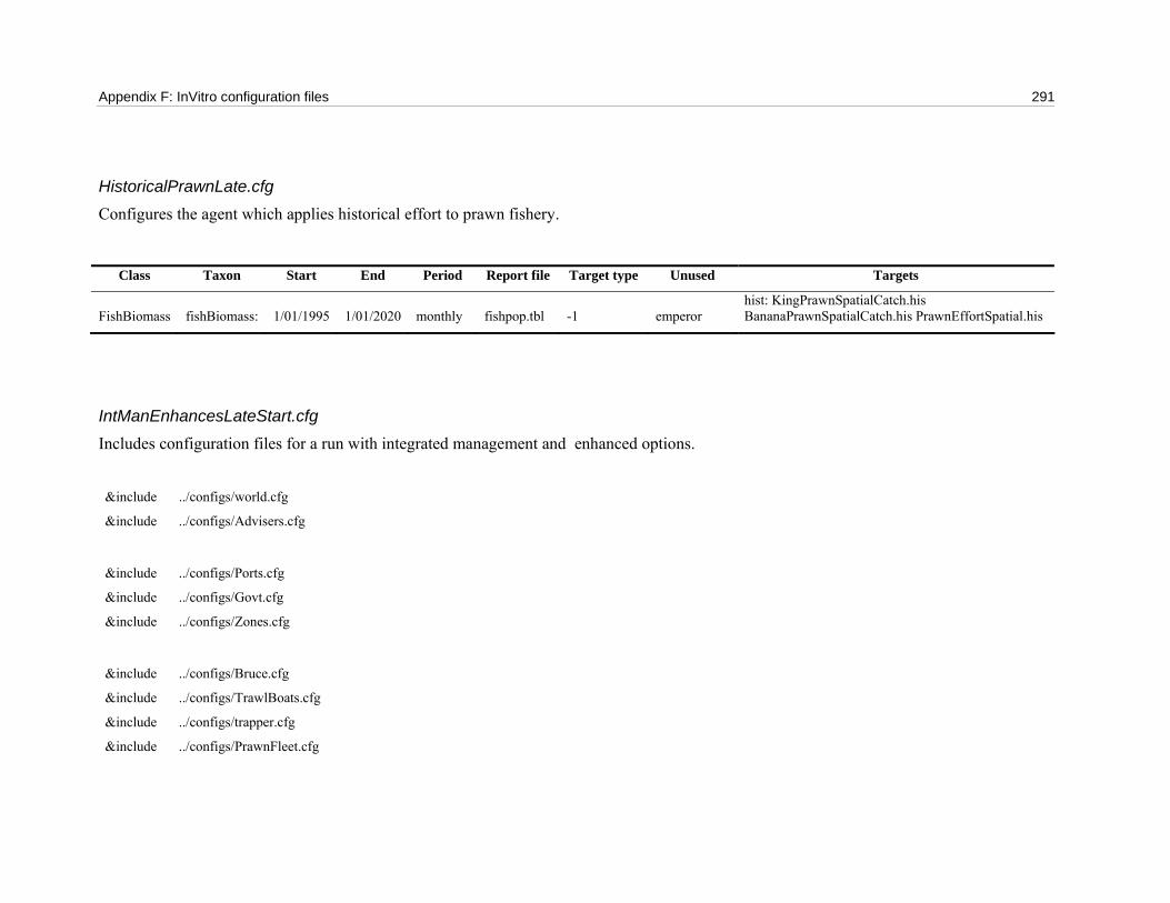
Appendix F: InVitro configuration files 291
HistoricalPrawnLate.cfg Configures the agent which applies historical effort to prawn fishery.
IntManEnhancesLateStart.cfg Includes configuration files for a run with integrated management and enhanced options.
&include ../configs/world.cfg
&include ../configs/Advisers.cfg
&include ../configs/Ports.cfg
&include ../configs/Govt.cfg
&include ../configs/Zones.cfg
&include ../configs/Bruce.cfg
&include ../configs/TrawlBoats.cfg
&include ../configs/trapper.cfg
&include ../configs/PrawnFleet.cfg
Class Taxon Start End Period Report file Target type Unused Targets
FishBiomass fishBiomass: 1/01/1995 1/01/2020 monthly fishpop.tbl -1 emperor hist: KingPrawnSpatialCatch.his BananaPrawnSpatialCatch.his PrawnEffortSpatial.his
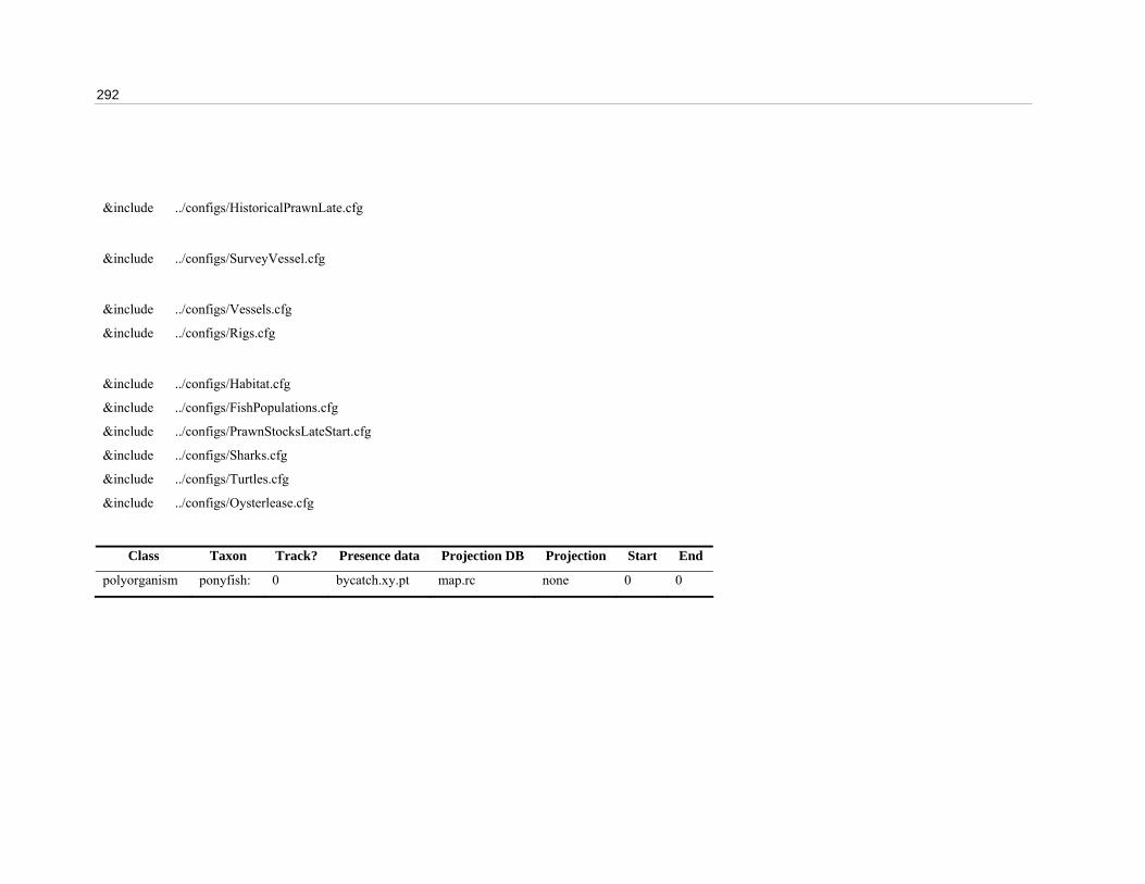
292
&include ../configs/HistoricalPrawnLate.cfg
&include ../configs/SurveyVessel.cfg
&include ../configs/Vessels.cfg
&include ../configs/Rigs.cfg
&include ../configs/Habitat.cfg
&include ../configs/FishPopulations.cfg
&include ../configs/PrawnStocksLateStart.cfg
&include ../configs/Sharks.cfg
&include ../configs/Turtles.cfg
&include ../configs/Oysterlease.cfg
Class Taxon Track? Presence data Projection DB Projection Start End
polyorganism ponyfish: 0 bycatch.xy.pt map.rc none 0 0
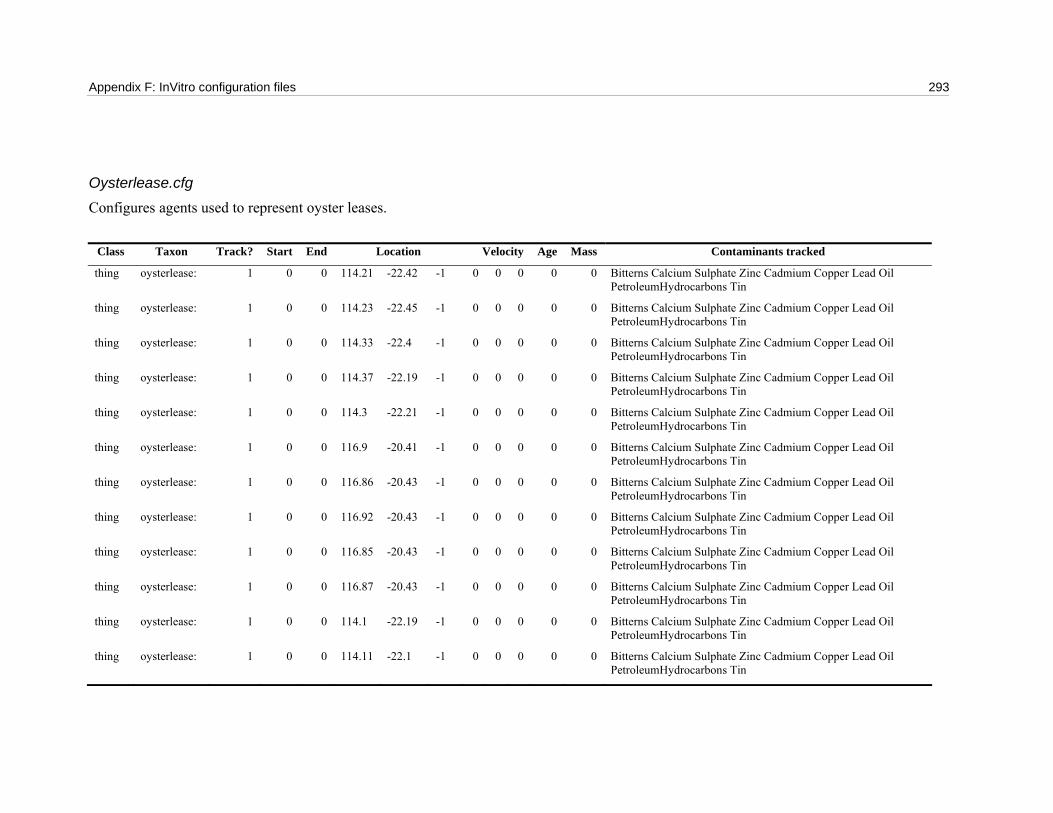
Appendix F: InVitro configuration files 293
Oysterlease.cfg Configures agents used to represent oyster leases.
Class Taxon Track? Start End Location Velocity Age Mass Contaminants tracked
thing oysterlease: 1 0 0 114.21 -22.42 -1 0 0 0 0 0 Bitterns Calcium Sulphate Zinc Cadmium Copper Lead Oil PetroleumHydrocarbons Tin
thing oysterlease: 1 0 0 114.23 -22.45 -1 0 0 0 0 0 Bitterns Calcium Sulphate Zinc Cadmium Copper Lead Oil PetroleumHydrocarbons Tin
thing oysterlease: 1 0 0 114.33 -22.4 -1 0 0 0 0 0 Bitterns Calcium Sulphate Zinc Cadmium Copper Lead Oil PetroleumHydrocarbons Tin
thing oysterlease: 1 0 0 114.37 -22.19 -1 0 0 0 0 0 Bitterns Calcium Sulphate Zinc Cadmium Copper Lead Oil PetroleumHydrocarbons Tin
thing oysterlease: 1 0 0 114.3 -22.21 -1 0 0 0 0 0 Bitterns Calcium Sulphate Zinc Cadmium Copper Lead Oil PetroleumHydrocarbons Tin
thing oysterlease: 1 0 0 116.9 -20.41 -1 0 0 0 0 0 Bitterns Calcium Sulphate Zinc Cadmium Copper Lead Oil PetroleumHydrocarbons Tin
thing oysterlease: 1 0 0 116.86 -20.43 -1 0 0 0 0 0 Bitterns Calcium Sulphate Zinc Cadmium Copper Lead Oil PetroleumHydrocarbons Tin
thing oysterlease: 1 0 0 116.92 -20.43 -1 0 0 0 0 0 Bitterns Calcium Sulphate Zinc Cadmium Copper Lead Oil PetroleumHydrocarbons Tin
thing oysterlease: 1 0 0 116.85 -20.43 -1 0 0 0 0 0 Bitterns Calcium Sulphate Zinc Cadmium Copper Lead Oil PetroleumHydrocarbons Tin
thing oysterlease: 1 0 0 116.87 -20.43 -1 0 0 0 0 0 Bitterns Calcium Sulphate Zinc Cadmium Copper Lead Oil PetroleumHydrocarbons Tin
thing oysterlease: 1 0 0 114.1 -22.19 -1 0 0 0 0 0 Bitterns Calcium Sulphate Zinc Cadmium Copper Lead Oil PetroleumHydrocarbons Tin
thing oysterlease: 1 0 0 114.11 -22.1 -1 0 0 0 0 0 Bitterns Calcium Sulphate Zinc Cadmium Copper Lead Oil PetroleumHydrocarbons Tin
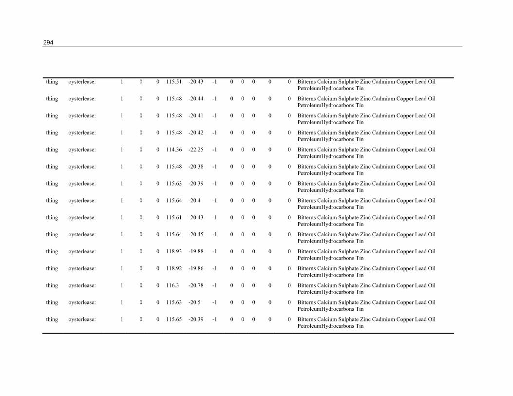
294
thing oysterlease: 1 0 0 115.51 -20.43 -1 0 0 0 0 0 Bitterns Calcium Sulphate Zinc Cadmium Copper Lead Oil PetroleumHydrocarbons Tin
thing oysterlease: 1 0 0 115.48 -20.44 -1 0 0 0 0 0 Bitterns Calcium Sulphate Zinc Cadmium Copper Lead Oil PetroleumHydrocarbons Tin
thing oysterlease: 1 0 0 115.48 -20.41 -1 0 0 0 0 0 Bitterns Calcium Sulphate Zinc Cadmium Copper Lead Oil PetroleumHydrocarbons Tin
thing oysterlease: 1 0 0 115.48 -20.42 -1 0 0 0 0 0 Bitterns Calcium Sulphate Zinc Cadmium Copper Lead Oil PetroleumHydrocarbons Tin
thing oysterlease: 1 0 0 114.36 -22.25 -1 0 0 0 0 0 Bitterns Calcium Sulphate Zinc Cadmium Copper Lead Oil PetroleumHydrocarbons Tin
thing oysterlease: 1 0 0 115.48 -20.38 -1 0 0 0 0 0 Bitterns Calcium Sulphate Zinc Cadmium Copper Lead Oil PetroleumHydrocarbons Tin
thing oysterlease: 1 0 0 115.63 -20.39 -1 0 0 0 0 0 Bitterns Calcium Sulphate Zinc Cadmium Copper Lead Oil PetroleumHydrocarbons Tin
thing oysterlease: 1 0 0 115.64 -20.4 -1 0 0 0 0 0 Bitterns Calcium Sulphate Zinc Cadmium Copper Lead Oil PetroleumHydrocarbons Tin
thing oysterlease: 1 0 0 115.61 -20.43 -1 0 0 0 0 0 Bitterns Calcium Sulphate Zinc Cadmium Copper Lead Oil PetroleumHydrocarbons Tin
thing oysterlease: 1 0 0 115.64 -20.45 -1 0 0 0 0 0 Bitterns Calcium Sulphate Zinc Cadmium Copper Lead Oil PetroleumHydrocarbons Tin
thing oysterlease: 1 0 0 118.93 -19.88 -1 0 0 0 0 0 Bitterns Calcium Sulphate Zinc Cadmium Copper Lead Oil PetroleumHydrocarbons Tin
thing oysterlease: 1 0 0 118.92 -19.86 -1 0 0 0 0 0 Bitterns Calcium Sulphate Zinc Cadmium Copper Lead Oil PetroleumHydrocarbons Tin
thing oysterlease: 1 0 0 116.3 -20.78 -1 0 0 0 0 0 Bitterns Calcium Sulphate Zinc Cadmium Copper Lead Oil PetroleumHydrocarbons Tin
thing oysterlease: 1 0 0 115.63 -20.5 -1 0 0 0 0 0 Bitterns Calcium Sulphate Zinc Cadmium Copper Lead Oil PetroleumHydrocarbons Tin
thing oysterlease: 1 0 0 115.65 -20.39 -1 0 0 0 0 0 Bitterns Calcium Sulphate Zinc Cadmium Copper Lead Oil PetroleumHydrocarbons Tin

Appendix F: InVitro configuration files 295
thing oysterlease: 1 0 0 115.64 -20.39 -1 0 0 0 0 0 Bitterns Calcium Sulphate Zinc Cadmium Copper Lead Oil PetroleumHydrocarbons Tin
thing oysterlease: 1 0 0 117.19 -20.6 -1 0 0 0 0 0 Bitterns Calcium Sulphate Zinc Cadmium Copper Lead Oil PetroleumHydrocarbons Tin
thing oysterlease: 1 0 0 118.49 -20.31 -1 0 0 0 0 0 Bitterns Calcium Sulphate Zinc Cadmium Copper Lead Oil PetroleumHydrocarbons Tin
thing oysterlease: 1 0 0 115.61 -20.39 -1 0 0 0 0 0 Bitterns Calcium Sulphate Zinc Cadmium Copper Lead Oil PetroleumHydrocarbons Tin
thing oysterlease: 1 0 0 115.62 -20.42 -1 0 0 0 0 0 Bitterns Calcium Sulphate Zinc Cadmium Copper Lead Oil PetroleumHydrocarbons Tin
thing oysterlease: 1 0 0 115.44 -20.43 -1 0 0 0 0 0 Bitterns Calcium Sulphate Zinc Cadmium Copper Lead Oil PetroleumHydrocarbons Tin
thing oysterlease: 1 0 0 115.45 -20.63 -1 0 0 0 0 0 Bitterns Calcium Sulphate Zinc Cadmium Copper Lead Oil PetroleumHydrocarbons Tin
thing oysterlease: 1 0 0 115.47 -20.64 -1 0 0 0 0 0 Bitterns Calcium Sulphate Zinc Cadmium Copper Lead Oil PetroleumHydrocarbons Tin
thing oysterlease: 1 0 0 116.18 -20.84 -1 0 0 0 0 0 Bitterns Calcium Sulphate Zinc Cadmium Copper Lead Oil PetroleumHydrocarbons Tin
thing oysterlease: 1 0 0 116.56 -20.55 -1 0 0 0 0 0 Bitterns Calcium Sulphate Zinc Cadmium Copper Lead Oil PetroleumHydrocarbons Tin
thing oysterlease: 1 0 0 115.52 -20.62 -1 0 0 0 0 0 Bitterns Calcium Sulphate Zinc Cadmium Copper Lead Oil PetroleumHydrocarbons Tin
thing oysterlease: 1 0 0 115.62 -20.39 -1 0 0 0 0 0 Bitterns Calcium Sulphate Zinc Cadmium Copper Lead Oil PetroleumHydrocarbons Tin
thing oysterlease: 1 0 0 117.67 -20.65 -1 0 0 0 0 0 Bitterns Calcium Sulphate Zinc Cadmium Copper Lead Oil PetroleumHydrocarbons Tin
thing oysterlease: 1 0 0 115.49 -21.43 -1 0 0 0 0 0 Bitterns Calcium Sulphate Zinc Cadmium Copper Lead Oil PetroleumHydrocarbons Tin
thing oysterlease: 1 0 0 115.68 -20.6 -1 0 0 0 0 0 Bitterns Calcium Sulphate Zinc Cadmium Copper Lead Oil PetroleumHydrocarbons Tin
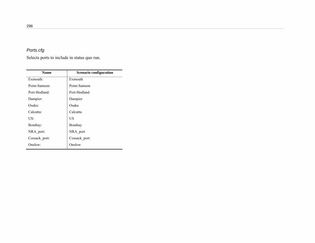
296
Ports.cfg Selects ports to include in status quo run.
Name Scenario configuration
Exmouth: Exmouth
Point-Samson: Point-Samson
Port-Hedland: Port-Hedland
Dampier: Dampier
Osaka: Osaka
Calcutta: Calcutta
US: US
Bombay: Bombay
NRA_port: NRA_port
Cossack_port: Cossack_port
Onslow: Onslow

Appendix F: InVitro configuration files 297
Ports_1p.cfg Selects ports to include in run with one development pulse.
Name Scenario configuration
Exmouth: Exmouth_1p
Point-Samson: Point-Samson
Port-Hedland: Port-Hedland_1p
Dampier: Dampier_1p
Osaka: Osaka
Calcutta: Calcutta
US: US
Bombay: Bombay
NRA_port: NRA_port
Cossack_port: Cossack_port
Onslow: Onslow_1p

298
Ports_2p.cfg Selects ports to include in run with two development pulses.
Name Scenario configuration
Exmouth: Exmouth_2p
Point-Samson: Point-Samson
Port-Hedland: Port-Hedland_2p
Dampier: Dampier_2p
Osaka: Osaka
Calcutta: Calcutta
US: US
Bombay: Bombay
NRA_port: NRA_port
Cossack_port: Cossack_port
Onslow: Onslow_2p

Appendix F: InVitro configuration files 299
PrawnFleet.cfg Configures the management authority and includes the spotter planes and fishing fleets for the status quo runs.
Class Management
Authority Start End Period Trawl zones Trap zones
Prawn zones Report file
Target class
Stock assessment data files
FMA fishWAFMA: 0 0 monthly pilbara-zones
pilbara-trap-zones
prawn-zones fishWAFMA.rpt T: boat
SAD: KingprawnNODAT.SAD
&include ../configs/planes.cfg
&include ../configs/ExmouthBoats.cfg
&include ../configs/OnslowBoats.cfg
&include ../configs/DampierBoats.cfg
PrawnFleet_1p.cfg Configures the management authority and includes the spotter planes and fishing fleets for the runs with one development pulse.
Class Management
Authority Start End Period Trawl zones Trap Zones
Prawn zones Report file
Enh. Mgmnt. Targets Stock assessment data files
FMA fishWAFMA: 0 0 monthly pilbara-zones
pilbara-trap-zones prawn-zones fishWAFMA.rpt 0 T: boat
SAD: KingprawnNODAT.SAD
BananaprawnNODAT.SAD

300
&include ../configs/planes.cfg
&include ../configs/ExmouthBoats_1p.cfg
&include ../configs/OnslowBoats_1p.cfg
&include ../configs/DampierBoats_1p.cfg
PrawnStocks.cfg Includes the king prawn and banana brawn stock files.
&include ../configs/Kingprawns.cfg
&include ../configs/Bananaprawns.cfg
PrawnStocksLateStart.cfg Includes the king prawn and banana brawn stock files.
&include ../configs/KingprawnsLateStart.cfg
&include ../configs/BananaprawnsLateStart.cfg

Appendix F: InVitro configuration files 301
Rigs.cfg Configures the platforms for Vessels to use as part of their itinerary.
Class Taxon Controller State of
Production Start End Unused Ununsed Unused Fishing
Restriction
oilco Ampule: 0
rig N_Rankin_A: Ampule 2 0 0 1.00E+12 1.00E+10 300 10000
rig Cossack: Ampule 2 0 0 1.00E+12 1.00E+10 300 10000
Sharks.cfg Configures agents which represent the shark population and agents to monitor them.
Class Taxon Starts Ends Sample interval Report file Target type Include blastula Only recruits Targets
biomass sharkesky: 0 0 monthly shark_bio.tbl 0 0 0 shark
Class Taxon Starts Ends Sample interval Report file Targets
tracker sharks: 0 0 monthly sharkmap shark
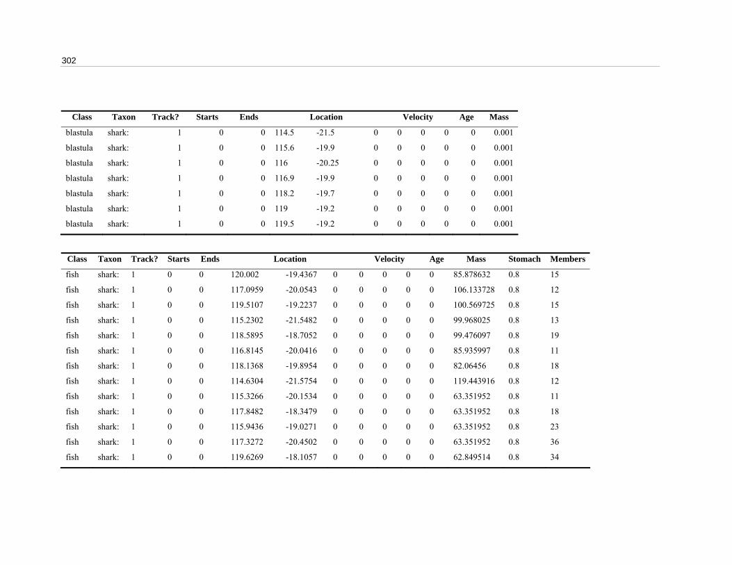
302
Class Taxon Track? Starts Ends Location Velocity Age Mass
blastula shark: 1 0 0 114.5 -21.5 0 0 0 0 0 0.001
blastula shark: 1 0 0 115.6 -19.9 0 0 0 0 0 0.001
blastula shark: 1 0 0 116 -20.25 0 0 0 0 0 0.001
blastula shark: 1 0 0 116.9 -19.9 0 0 0 0 0 0.001
blastula shark: 1 0 0 118.2 -19.7 0 0 0 0 0 0.001
blastula shark: 1 0 0 119 -19.2 0 0 0 0 0 0.001
blastula shark: 1 0 0 119.5 -19.2 0 0 0 0 0 0.001
Class Taxon Track? Starts Ends Location Velocity Age Mass Stomach Members
fish shark: 1 0 0 120.002 -19.4367 0 0 0 0 0 85.878632 0.8 15
fish shark: 1 0 0 117.0959 -20.0543 0 0 0 0 0 106.133728 0.8 12
fish shark: 1 0 0 119.5107 -19.2237 0 0 0 0 0 100.569725 0.8 15
fish shark: 1 0 0 115.2302 -21.5482 0 0 0 0 0 99.968025 0.8 13
fish shark: 1 0 0 118.5895 -18.7052 0 0 0 0 0 99.476097 0.8 19
fish shark: 1 0 0 116.8145 -20.0416 0 0 0 0 0 85.935997 0.8 11
fish shark: 1 0 0 118.1368 -19.8954 0 0 0 0 0 82.06456 0.8 18
fish shark: 1 0 0 114.6304 -21.5754 0 0 0 0 0 119.443916 0.8 12
fish shark: 1 0 0 115.3266 -20.1534 0 0 0 0 0 63.351952 0.8 11
fish shark: 1 0 0 117.8482 -18.3479 0 0 0 0 0 63.351952 0.8 18
fish shark: 1 0 0 115.9436 -19.0271 0 0 0 0 0 63.351952 0.8 23
fish shark: 1 0 0 117.3272 -20.4502 0 0 0 0 0 63.351952 0.8 36
fish shark: 1 0 0 119.6269 -18.1057 0 0 0 0 0 62.849514 0.8 34

Appendix F: InVitro configuration files 303
Class Taxon Track? Starts Ends Location Velocity Age Mass Stomach Members
fish shark: 1 0 0 119.7441 -19.5313 0 0 0 0 0 60.346157 0.8 25
fish shark: 1 0 0 118.2556 -19.6129 0 0 0 0 0 60.346157 0.8 17
fish shark: 1 0 0 119.8787 -19.3509 0 0 0 0 0 60.346157 0.8 18
fish shark: 1 0 0 118.9035 -17.6088 0 0 0 0 0 60.346157 0.8 27
fish shark: 1 0 0 117.9114 -18.4388 0 0 0 0 0 60.346157 0.8 16
fish shark: 1 0 0 115.8507 -20.1111 0 0 0 0 0 60.346157 0.8 17
fish shark: 1 0 0 119.2918 -19.3417 0 0 0 0 0 58.824387 0.8 15
fish shark: 1 0 0 117.4845 -20.2108 0 0 0 0 0 58.824387 0.8 24
fish shark: 1 0 0 119.291 -19.0697 0 0 0 0 0 58.824387 0.8 28
fish shark: 1 0 0 114.5649 -21.5161 0 0 0 0 0 58.210415 0.8 29
fish shark: 1 0 0 119.9001 -18.3057 0 0 0 0 0 58.210415 0.8 18
fish shark: 1 0 0 119.1814 -19.2817 0 0 0 0 0 58.210415 0.8 26
fish shark: 1 0 0 119.7607 -19.0187 0 0 0 0 0 58.210415 0.8 32
fish shark: 1 0 0 116.8309 -18.9823 0 0 0 0 0 55.742508 0.8 10
fish shark: 1 0 0 119.3422 -18.0505 0 0 0 0 0 55.742508 0.8 29
fish shark: 1 0 0 118.4656 -19.0188 0 0 0 0 0 55.742508 0.8 21
fish shark: 1 0 0 117.536 -19.9403 0 0 0 0 0 55.742508 0.8 19
fish shark: 1 0 0 119.5919 -17.5282 0 0 0 0 0 55.742508 0.8 23
fish shark: 1 0 0 115.7294 -20.4154 0 0 0 0 0 54.182186 0.8 11
fish shark: 1 0 0 119.6146 -18.3839 0 0 0 0 0 54.182186 0.8 30
fish shark: 1 0 0 118.8989 -18.8051 0 0 0 0 0 54.182186 0.8 15
fish shark: 1 0 0 115.0073 -20.9704 0 0 0 0 0 54.182186 0.8 21
fish shark: 1 0 0 118.1389 -19.5197 0 0 0 0 0 50.379314 0.8 27

304
Class Taxon Track? Starts Ends Location Velocity Age Mass Stomach Members
fish shark: 1 0 0 116.8683 -20.1819 0 0 0 0 0 49.422482 0.8 36
fish shark: 1 0 0 114.2135 -21.7871 0 0 0 0 0 49.422482 0.8 18
fish shark: 1 0 0 117.4632 -20.2049 0 0 0 0 0 49.422482 0.8 45
fish shark: 1 0 0 119.3028 -18.1487 0 0 0 0 0 48.576935 0.8 15
fish shark: 1 0 0 119.3941 -18.6227 0 0 0 0 0 48.576935 0.8 12
fish shark: 1 0 0 117.8045 -19.4329 0 0 0 0 0 48.576935 0.8 14
fish shark: 1 0 0 119.5401 -17.9087 0 0 0 0 0 48.576935 0.8 23
fish shark: 1 0 0 119.7424 -18.8365 0 0 0 0 0 48.576935 0.8 26
fish shark: 1 0 0 114.3651 -21.8609 0 0 0 0 0 46.182594 0.8 16
fish shark: 1 0 0 116.1608 -20.6089 0 0 0 0 0 46.182594 0.8 12
fish shark: 1 0 0 119.0563 -19.79 0 0 0 0 0 46.182594 0.8 22
fish shark: 1 0 0 119.6136 -19.7177 0 0 0 0 0 44.542305 0.8 25
fish shark: 1 0 0 119.9711 -17.6275 0 0 0 0 0 43.576527 0.8 19
fish shark: 1 0 0 118.476 -19.899 0 0 0 0 0 43.576527 0.8 23
fish shark: 1 0 0 118.3335 -17.9338 0 0 0 0 0 41.220371 0.8 25
fish shark: 1 0 0 118.1118 -18.2672 0 0 0 0 0 41.220371 0.8 17
fish shark: 1 0 0 118.3315 -18.452 0 0 0 0 0 41.220371 0.8 20
fish shark: 1 0 0 117.4507 -20.2414 0 0 0 0 0 41.220371 0.8 26
fish shark: 1 0 0 117.0706 -20.6029 0 0 0 0 0 39.539227 0.8 16
fish shark: 1 0 0 118.3879 -20.2359 0 0 0 0 0 39.539227 0.8 19
fish shark: 1 0 0 118.4992 -20.0295 0 0 0 0 0 38.449528 0.8 16
fish shark: 1 0 0 116.2447 -19.8815 0 0 0 0 0 38.449528 0.8 17
fish shark: 1 0 0 114.8738 -21.1162 0 0 0 0 0 38.449528 0.8 20

Appendix F: InVitro configuration files 305
Class Taxon Track? Starts Ends Location Velocity Age Mass Stomach Members
fish shark: 1 0 0 118.652 -19.3325 0 0 0 0 0 37.983631 0.8 26
fish shark: 1 0 0 117.624 -19.7288 0 0 0 0 0 37.983631 0.8 32
fish shark: 1 0 0 117.1627 -20.1932 0 0 0 0 0 37.983631 0.8 29
fish shark: 1 0 0 115.7665 -20.0564 0 0 0 0 0 37.983631 0.8 24
fish shark: 1 0 0 115.5464 -20.9375 0 0 0 0 0 37.983631 0.8 25
fish shark: 1 0 0 114.551 -21.6328 0 0 0 0 0 37.983631 0.8 25
fish shark: 1 0 0 116.1684 -20.8117 0 0 0 0 0 37.743969 0.8 20
fish shark: 1 0 0 119.2431 -19.8212 0 0 0 0 0 37.743969 0.8 20
fish shark: 1 0 0 118.3269 -18.2015 0 0 0 0 0 37.743969 0.8 20
fish shark: 1 0 0 118.095 -19.684 0 0 0 0 0 37.743969 0.8 16
fish shark: 1 0 0 115.583 -20.584 0 0 0 0 0 36.132534 0.8 25
fish shark: 1 0 0 116.4735 -19.2776 0 0 0 0 0 36.132534 0.8 30
fish shark: 1 0 0 118.8795 -19.5798 0 0 0 0 0 36.132534 0.8 20
fish shark: 1 0 0 117.7623 -20.4718 0 0 0 0 0 36.184269 0.8 19
fish shark: 1 0 0 118.9234 -19.3776 0 0 0 0 0 35.971828 0.8 15
fish shark: 1 0 0 118.1877 -18.2582 0 0 0 0 0 35.971828 0.8 15
fish shark: 1 0 0 119.8503 -18.1877 0 0 0 0 0 34.397064 0.8 15
fish shark: 1 0 0 119.1467 -17.4931 0 0 0 0 0 34.397064 0.8 15
fish shark: 1 0 0 117.153 -20.2367 0 0 0 0 0 34.397064 0.8 15
fish shark: 1 0 0 115.1793 -20.3425 0 0 0 0 0 34.397064 0.8 15
fish shark: 1 0 0 117.3984 -20.5921 0 0 0 0 0 34.217525 0.8 29
fish shark: 1 0 0 115.5722 -20.5402 0 0 0 0 0 34.217525 0.8 29
fish shark: 1 0 0 118.1918 -20.3326 0 0 0 0 0 34.217525 0.8 31
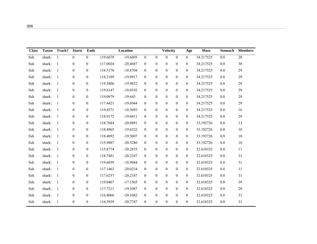
306
Class Taxon Track? Starts Ends Location Velocity Age Mass Stomach Members
fish shark: 1 0 0 119.6679 -19.6695 0 0 0 0 0 34.217525 0.8 28
fish shark: 1 0 0 117.0024 -20.4687 0 0 0 0 0 34.217525 0.8 30
fish shark: 1 0 0 118.5176 -18.8704 0 0 0 0 0 34.217525 0.8 29
fish shark: 1 0 0 118.2189 -19.0917 0 0 0 0 0 34.217525 0.8 29
fish shark: 1 0 0 119.5806 -19.9832 0 0 0 0 0 34.217525 0.8 29
fish shark: 1 0 0 119.8147 -18.0192 0 0 0 0 0 34.217525 0.8 29
fish shark: 1 0 0 119.0979 -19.643 0 0 0 0 0 34.217525 0.8 29
fish shark: 1 0 0 117.4421 -19.6944 0 0 0 0 0 34.217525 0.8 29
fish shark: 1 0 0 119.8571 -18.5693 0 0 0 0 0 34.217525 0.8 16
fish shark: 1 0 0 118.9172 -19.0411 0 0 0 0 0 34.217525 0.8 29
fish shark: 1 0 0 118.7684 -20.0891 0 0 0 0 0 33.192726 0.8 13
fish shark: 1 0 0 118.4965 -19.6322 0 0 0 0 0 33.192726 0.8 10
fish shark: 1 0 0 118.4092 -19.5607 0 0 0 0 0 33.192726 0.8 10
fish shark: 1 0 0 115.9887 -20.5286 0 0 0 0 0 33.192726 0.8 10
fish shark: 1 0 0 115.8774 -20.2835 0 0 0 0 0 32.610325 0.8 11
fish shark: 1 0 0 118.7481 -20.2347 0 0 0 0 0 32.610325 0.8 31
fish shark: 1 0 0 119.6039 -18.9684 0 0 0 0 0 32.610325 0.8 31
fish shark: 1 0 0 117.1463 -20.0234 0 0 0 0 0 32.610325 0.8 11
fish shark: 1 0 0 117.6257 -20.2187 0 0 0 0 0 32.610325 0.8 31
fish shark: 1 0 0 119.0467 -17.1565 0 0 0 0 0 32.610325 0.8 39
fish shark: 1 0 0 117.7211 -19.1087 0 0 0 0 0 32.610325 0.8 20
fish shark: 1 0 0 116.4066 -20.1082 0 0 0 0 0 32.610325 0.8 31
fish shark: 1 0 0 116.3939 -20.7747 0 0 0 0 0 32.610325 0.8 31

Appendix F: InVitro configuration files 307
Class Taxon Track? Starts Ends Location Velocity Age Mass Stomach Members
fish shark: 1 0 0 115.1355 -20.9913 0 0 0 0 0 32.382988 0.8 31
fish shark: 1 0 0 119.8325 -19.5564 0 0 0 0 0 32.382988 0.8 24
fish shark: 1 0 0 116.76 -19.6334 0 0 0 0 0 32.382988 0.8 31
fish shark: 1 0 0 118.0865 -18.7733 0 0 0 0 0 32.382988 0.8 31
fish shark: 1 0 0 117.5836 -18.4952 0 0 0 0 0 32.382988 0.8 30
fish shark: 1 0 0 116.2092 -19.58 0 0 0 0 0 32.382988 0.8 30
fish shark: 1 0 0 116.4975 -20.3652 0 0 0 0 0 32.382988 0.8 27
fish shark: 1 0 0 115.0098 -21.2211 0 0 0 0 0 32.382988 0.8 29
fish shark: 1 0 0 114.7459 -20.8057 0 0 0 0 0 32.382988 0.8 29
fish shark: 1 0 0 115.7726 -20.9985 0 0 0 0 0 30.806532 0.8 19
fish shark: 1 0 0 119.6744 -18.3625 0 0 0 0 0 30.806532 0.8 19
fish shark: 1 0 0 118.8756 -19.7525 0 0 0 0 0 30.806532 0.8 19
fish shark: 1 0 0 117.9728 -19.1995 0 0 0 0 0 30.806532 0.8 33
fish shark: 1 0 0 118.1819 -20.083 0 0 0 0 0 30.806532 0.8 29
fish shark: 1 0 0 117.8028 -20.4167 0 0 0 0 0 30.806532 0.8 19
fish shark: 1 0 0 118.7245 -19.0119 0 0 0 0 0 30.806532 0.8 33
fish shark: 1 0 0 119.1359 -19.091 0 0 0 0 0 30.806532 0.8 18
fish shark: 1 0 0 118.7984 -18.2686 0 0 0 0 0 28.972282 0.8 36
fish shark: 1 0 0 119.4618 -17.4036 0 0 0 0 0 28.972282 0.8 36
fish shark: 1 0 0 118.5937 -17.6361 0 0 0 0 0 28.972282 0.8 42
fish shark: 1 0 0 117.4673 -20.3899 0 0 0 0 0 28.972282 0.8 41
fish shark: 1 0 0 119.0921 -19.8983 0 0 0 0 0 28.972282 0.8 45
fish shark: 1 0 0 118.4438 -18.4977 0 0 0 0 0 28.788021 0.8 36

308
Class Taxon Track? Starts Ends Location Velocity Age Mass Stomach Members
fish shark: 1 0 0 119.7647 -19.6736 0 0 0 0 0 28.788021 0.8 36
fish shark: 1 0 0 117.6373 -18.4822 0 0 0 0 0 28.788021 0.8 21
fish shark: 1 0 0 114.7666 -21.2878 0 0 0 0 0 28.788021 0.8 36
fish shark: 1 0 0 119.559 -18.15 0 0 0 0 0 28.788021 0.8 36
fish shark: 1 0 0 115.9993 -20.8186 0 0 0 0 0 28.788021 0.8 36
fish shark: 1 0 0 114.7209 -21.2984 0 0 0 0 0 28.788021 0.8 36
fish shark: 1 0 0 118.379 -19.6575 0 0 0 0 0 28.788021 0.8 32
fish shark: 1 0 0 118.7398 -20.0261 0 0 0 0 0 28.788021 0.8 36
fish shark: 1 0 0 116.8722 -20.1832 0 0 0 0 0 28.788021 0.8 36
fish shark: 1 0 0 118.336 -18.9263 0 0 0 0 0 28.788021 0.8 32
fish shark: 1 0 0 115.5545 -20.7356 0 0 0 0 0 28.788021 0.8 32
fish shark: 1 0 0 118.2241 -18.3924 0 0 0 0 0 28.788021 0.8 32
fish shark: 1 0 0 117.6559 -18.8017 0 0 0 0 0 28.234297 0.8 31
fish shark: 1 0 0 116.451 -19.5671 0 0 0 0 0 27.122686 0.8 39
fish shark: 1 0 0 118.3622 -18.4304 0 0 0 0 0 27.122686 0.8 39
fish shark: 1 0 0 119.3348 -19.7459 0 0 0 0 0 27.122686 0.8 39
fish shark: 1 0 0 116.0878 -20.0398 0 0 0 0 0 27.122686 0.8 18
fish shark: 1 0 0 118.2377 -19.2905 0 0 0 0 0 27.122686 0.8 34
fish shark: 1 0 0 119.2856 -19.9403 0 0 0 0 0 27.122686 0.8 39
fish shark: 1 0 0 117.486 -20.3578 0 0 0 0 0 26.93688 0.8 39
fish shark: 1 0 0 119.8798 -19.4928 0 0 0 0 0 26.93688 0.8 39
fish shark: 1 0 0 118.8215 -19.1958 0 0 0 0 0 26.93688 0.8 30
fish shark: 1 0 0 119.3972 -19.2899 0 0 0 0 0 26.93688 0.8 38
Appendix F: InVitro configuration files 309
Class Taxon Track? Starts Ends Location Velocity Age Mass Stomach Members
fish shark: 1 0 0 119.6933 -19.3587 0 0 0 0 0 26.93688 0.8 30
fish shark: 1 0 0 117.5246 -18.9017 0 0 0 0 0 26.93688 0.8 39
fish shark: 1 0 0 119.9678 -19.4723 0 0 0 0 0 26.93688 0.8 30
fish shark: 1 0 0 118.283 -18.6088 0 0 0 0 0 26.93688 0.8 39
fish shark: 1 0 0 114.7847 -21.551 0 0 0 0 0 26.93688 0.8 39
fish shark: 1 0 0 115.5075 -19.6394 0 0 0 0 0 26.93688 0.8 30
fish shark: 1 0 0 118.3531 -18.7653 0 0 0 0 0 26.93688 0.8 39
fish shark: 1 0 0 115.2746 -20.9342 0 0 0 0 0 26.93688 0.8 39
fish shark: 1 0 0 119.5282 -19.5697 0 0 0 0 0 26.93688 0.8 30
fish shark: 1 0 0 119.1812 -19.258 0 0 0 0 0 26.93688 0.8 30
fish shark: 1 0 0 114.8874 -20.644 0 0 0 0 0 26.93688 0.8 39
fish shark: 1 0 0 119.6514 -19.4967 0 0 0 0 0 26.93688 0.8 39
fish shark: 1 0 0 116.6783 -19.3728 0 0 0 0 0 26.378531 0.8 31
fish shark: 1 0 0 117.8754 -19.2067 0 0 0 0 0 26.378531 0.8 32
fish shark: 1 0 0 119.7983 -18.2415 0 0 0 0 0 25.25762 0.8 42
fish shark: 1 0 0 118.8839 -17.9025 0 0 0 0 0 25.25762 0.8 42
fish shark: 1 0 0 119.1365 -19.7819 0 0 0 0 0 25.25762 0.8 42
fish shark: 1 0 0 114.7391 -20.7481 0 0 0 0 0 25.25762 0.8 45
fish shark: 1 0 0 114.6493 -21.6042 0 0 0 0 0 25.070255 0.8 39
fish shark: 1 0 0 118.3914 -19.2639 0 0 0 0 0 25.070255 0.8 25
fish shark: 1 0 0 117.3102 -20.4621 0 0 0 0 0 25.070255 0.8 42
fish shark: 1 0 0 115.815 -20.9198 0 0 0 0 0 25.070255 0.8 25
fish shark: 1 0 0 117.8208 -18.6478 0 0 0 0 0 25.070255 0.8 42

310
Class Taxon Track? Starts Ends Location Velocity Age Mass Stomach Members
fish shark: 1 0 0 115.5055 -21.2702 0 0 0 0 0 25.070255 0.8 25
fish shark: 1 0 0 113.7122 -22.8893 0 0 0 0 0 25.070255 0.8 42
fish shark: 1 0 0 119.7824 -19.3468 0 0 0 0 0 25.070255 0.8 42
fish shark: 1 0 0 118.8725 -19.6162 0 0 0 0 0 25.070255 0.8 23
fish shark: 1 0 0 114.165 -22.0258 0 0 0 0 0 25.070255 0.8 42
fish shark: 1 0 0 115.4497 -20.8572 0 0 0 0 0 25.070255 0.8 25
fish shark: 1 0 0 117.8891 -19.7623 0 0 0 0 0 25.070255 0.8 42
fish shark: 1 0 0 116.5971 -20.5617 0 0 0 0 0 25.070255 0.8 25
fish shark: 1 0 0 117.9762 -19.1085 0 0 0 0 0 25.070255 0.8 42
fish shark: 1 0 0 117.5351 -18.6928 0 0 0 0 0 25.070255 0.8 25
fish shark: 1 0 0 119.0615 -18.6143 0 0 0 0 0 23.376945 0.8 45
fish shark: 1 0 0 118.5365 -20.295 0 0 0 0 0 23.376945 0.8 45
fish shark: 1 0 0 117.0688 -20.4305 0 0 0 0 0 23.376945 0.8 45
fish shark: 1 0 0 117.668 -18.9773 0 0 0 0 0 23.376945 0.8 45
fish shark: 1 0 0 119.8007 -19.892 0 0 0 0 0 23.376945 0.8 45
fish shark: 1 0 0 114.1712 -22.1677 0 0 0 0 0 23.376945 0.8 45
fish shark: 1 0 0 118.0082 -19.1426 0 0 0 0 0 23.188013 0.8 43
fish shark: 1 0 0 117.279 -20.4136 0 0 0 0 0 23.188013 0.8 46
fish shark: 1 0 0 118.2406 -19.6241 0 0 0 0 0 23.188013 0.8 41
fish shark: 1 0 0 119.594 -18.6281 0 0 0 0 0 23.188013 0.8 46
fish shark: 1 0 0 116.9036 -20.5291 0 0 0 0 0 23.188013 0.8 42
fish shark: 1 0 0 114.3518 -21.7433 0 0 0 0 0 23.188013 0.8 45
fish shark: 1 0 0 118.3612 -18.4251 0 0 0 0 0 23.188013 0.8 43
Appendix F: InVitro configuration files 311
Class Taxon Track? Starts Ends Location Velocity Age Mass Stomach Members
fish shark: 1 0 0 119.1582 -18.7959 0 0 0 0 0 23.188013 0.8 42
fish shark: 1 0 0 118.9829 -18.679 0 0 0 0 0 23.188013 0.8 46
fish shark: 1 0 0 117.2008 -19.5119 0 0 0 0 0 21.480524 0.8 49
fish shark: 1 0 0 117.1112 -20.1294 0 0 0 0 0 21.480524 0.8 11
fish shark: 1 0 0 114.4649 -21.885 0 0 0 0 0 21.480524 0.8 49
fish shark: 1 0 0 117.4991 -20.1355 0 0 0 0 0 21.480524 0.8 11
fish shark: 1 0 0 119.7821 -17.8264 0 0 0 0 0 21.480524 0.8 11
fish shark: 1 0 0 119.8655 -19.428 0 0 0 0 0 21.480524 0.8 49
fish shark: 1 0 0 115.3562 -21.4221 0 0 0 0 0 21.480524 0.8 11
fish shark: 1 0 0 119.421 -17.8295 0 0 0 0 0 21.290009 0.8 27
fish shark: 1 0 0 117.7829 -18.587 0 0 0 0 0 21.290009 0.8 49
fish shark: 1 0 0 119.0669 -18.6755 0 0 0 0 0 21.290009 0.8 49
fish shark: 1 0 0 116.5531 -20.5239 0 0 0 0 0 21.290009 0.8 49
fish shark: 1 0 0 119.7934 -19.9239 0 0 0 0 0 21.290009 0.8 49
fish shark: 1 0 0 119.5567 -19.3822 0 0 0 0 0 21.290009 0.8 27
fish shark: 1 0 0 118.9485 -17.5193 0 0 0 0 0 21.290009 0.8 49
fish shark: 1 0 0 119.3541 -19.3184 0 0 0 0 0 21.290009 0.8 49
fish shark: 1 0 0 115.4619 -20.0165 0 0 0 0 0 21.290009 0.8 48
fish shark: 1 0 0 116.4441 -20.2831 0 0 0 0 0 21.290009 0.8 27
fish shark: 1 0 0 119.2601 -19.4638 0 0 0 0 0 21.290009 0.8 49
fish shark: 1 0 0 115.6027 -20.73 0 0 0 0 0 21.290009 0.8 49
fish shark: 1 0 0 115.4333 -19.8392 0 0 0 0 0 21.290009 0.8 27
fish shark: 1 0 0 116.5066 -20.6297 0 0 0 0 0 20.71752 0.8 30

312
Class Taxon Track? Starts Ends Location Velocity Age Mass Stomach Members
fish shark: 1 0 0 117.9706 -19.2466 0 0 0 0 0 19.568239 0.8 53
fish shark: 1 0 0 119.1318 -18.8158 0 0 0 0 0 19.568239 0.8 10
fish shark: 1 0 0 119.311 -18.2262 0 0 0 0 0 19.568239 0.8 50
fish shark: 1 0 0 119.541 -19.9114 0 0 0 0 0 19.568239 0.8 10
fish shark: 1 0 0 118.1473 -19.6178 0 0 0 0 0 19.568239 0.8 53
fish shark: 1 0 0 119.4121 -17.8919 0 0 0 0 0 19.568239 0.8 53
fish shark: 1 0 0 118.8301 -20.113 0 0 0 0 0 19.568239 0.8 46
fish shark: 1 0 0 119.0781 -19.3355 0 0 0 0 0 19.568239 0.8 10
fish shark: 1 0 0 115.6238 -20.043 0 0 0 0 0 19.376127 0.8 53
fish shark: 1 0 0 115.062 -21.4816 0 0 0 0 0 19.376127 0.8 53
fish shark: 1 0 0 118.9421 -18.9017 0 0 0 0 0 19.376127 0.8 29
fish shark: 1 0 0 117.5134 -20.4163 0 0 0 0 0 19.376127 0.8 53
fish shark: 1 0 0 115.6209 -20.1095 0 0 0 0 0 19.376127 0.8 53
fish shark: 1 0 0 118.514 -17.8244 0 0 0 0 0 19.376127 0.8 53
fish shark: 1 0 0 119.812 -18.3305 0 0 0 0 0 19.376127 0.8 53
fish shark: 1 0 0 114.326 -22.1464 0 0 0 0 0 19.376127 0.8 29
fish shark: 1 0 0 117.7399 -18.4483 0 0 0 0 0 19.376127 0.8 53
fish shark: 1 0 0 117.0343 -19.8129 0 0 0 0 0 19.376127 0.8 53
fish shark: 1 0 0 115.8965 -20.332 0 0 0 0 0 19.376127 0.8 25
fish shark: 1 0 0 116.3799 -19.4965 0 0 0 0 0 19.376127 0.8 53
fish shark: 1 0 0 119.3439 -19.4864 0 0 0 0 0 19.376127 0.8 53
fish shark: 1 0 0 117.3055 -20.3922 0 0 0 0 0 19.376127 0.8 29
fish shark: 1 0 0 118.6623 -19.7323 0 0 0 0 0 19.376127 0.8 53

Appendix F: InVitro configuration files 313
Class Taxon Track? Starts Ends Location Velocity Age Mass Stomach Members
fish shark: 1 0 0 115.2897 -20.9502 0 0 0 0 0 19.376127 0.8 53
fish shark: 1 0 0 119.525 -17.5512 0 0 0 0 0 19.376127 0.8 29
fish shark: 1 0 0 115.5272 -19.4935 0 0 0 0 0 19.376127 0.8 53
fish shark: 1 0 0 118.9648 -17.9362 0 0 0 0 0 19.376127 0.8 53
fish shark: 1 0 0 115.271 -21.0502 0 0 0 0 0 19.376127 0.8 29
fish shark: 1 0 0 116.3261 -19.8535 0 0 0 0 0 17.639948 0.8 54
fish shark: 1 0 0 119.9168 -18.5014 0 0 0 0 0 17.446236 0.8 29
fish shark: 1 0 0 119.3731 -19.6822 0 0 0 0 0 17.446236 0.8 29
fish shark: 1 0 0 119.2319 -18.5144 0 0 0 0 0 17.446236 0.8 29
fish shark: 1 0 0 118.9297 -18.1482 0 0 0 0 0 17.446236 0.8 29
fish shark: 1 0 0 116.9382 -20.5551 0 0 0 0 0 17.446236 0.8 29
fish shark: 1 0 0 115.3706 -20.3688 0 0 0 0 0 16.864126 0.8 36
fish shark: 1 0 0 115.1398 -21.3925 0 0 0 0 0 15.695527 0.8 58
fish shark: 1 0 0 117.5297 -20.3992 0 0 0 0 0 15.695527 0.8 58
fish shark: 1 0 0 118.3084 -19.9598 0 0 0 0 0 15.695527 0.8 58
fish shark: 1 0 0 118.0463 -20.1944 0 0 0 0 0 15.695527 0.8 58
fish shark: 1 0 0 116.5034 -19.8333 0 0 0 0 0 15.695527 0.8 46
fish shark: 1 0 0 116.8371 -19.5543 0 0 0 0 0 15.695527 0.8 58
fish shark: 1 0 0 119.7512 -19.2036 0 0 0 0 0 15.695527 0.8 58
fish shark: 1 0 0 118.2091 -19.2086 0 0 0 0 0 15.500193 0.8 59
fish shark: 1 0 0 115.9383 -20.7085 0 0 0 0 0 15.500193 0.8 62
fish shark: 1 0 0 114.9485 -21.4181 0 0 0 0 0 15.500193 0.8 16
fish shark: 1 0 0 114.3 -22.1252 0 0 0 0 0 15.500193 0.8 14
314
Class Taxon Track? Starts Ends Location Velocity Age Mass Stomach Members
fish shark: 1 0 0 118.9016 -18.3053 0 0 0 0 0 15.500193 0.8 16
fish shark: 1 0 0 114.539 -21.593 0 0 0 0 0 15.500193 0.8 62
fish shark: 1 0 0 116.4811 -20.6426 0 0 0 0 0 15.500193 0.8 62
fish shark: 1 0 0 118.5327 -19.6935 0 0 0 0 0 15.500193 0.8 16
fish shark: 1 0 0 114.23 -21.1885 0 0 0 0 0 15.500193 0.8 62
fish shark: 1 0 0 118.6752 -18.7744 0 0 0 0 0 15.500193 0.8 62
fish shark: 1 0 0 114.2077 -22.2425 0 0 0 0 0 15.500193 0.8 16
fish shark: 1 0 0 119.054 -18.6964 0 0 0 0 0 15.500193 0.8 62
fish shark: 1 0 0 114.1694 -21.1074 0 0 0 0 0 15.500193 0.8 62
fish shark: 1 0 0 115.0122 -21.365 0 0 0 0 0 15.500193 0.8 56
fish shark: 1 0 0 114.3001 -21.9198 0 0 0 0 0 14.913207 0.8 49
fish shark: 1 0 0 118.7512 -20.0318 0 0 0 0 0 13.734832 0.8 60
fish shark: 1 0 0 116.4609 -20.0828 0 0 0 0 0 13.734832 0.8 60
fish shark: 1 0 0 119.494 -18.7829 0 0 0 0 0 13.734832 0.8 60
fish shark: 1 0 0 117.4797 -19.9956 0 0 0 0 0 13.734832 0.8 60
fish shark: 1 0 0 114.6013 -21.4851 0 0 0 0 0 13.734832 0.8 60
fish shark: 1 0 0 118.8216 -20.0278 0 0 0 0 0 13.734832 0.8 60
fish shark: 1 0 0 118.1301 -18.9493 0 0 0 0 0 13.734832 0.8 52
fish shark: 1 0 0 118.555 -19.9889 0 0 0 0 0 13.537864 0.8 67
fish shark: 1 0 0 115.8567 -20.1287 0 0 0 0 0 13.537864 0.8 67
fish shark: 1 0 0 115.6038 -21.0547 0 0 0 0 0 13.537864 0.8 17
fish shark: 1 0 0 115.9707 -19.6101 0 0 0 0 0 13.537864 0.8 67
fish shark: 1 0 0 115.8199 -20.0922 0 0 0 0 0 13.537864 0.8 67

Appendix F: InVitro configuration files 315
Class Taxon Track? Starts Ends Location Velocity Age Mass Stomach Members
fish shark: 1 0 0 115.6088 -20.102 0 0 0 0 0 13.537864 0.8 20
fish shark: 1 0 0 118.4868 -19.0912 0 0 0 0 0 13.537864 0.8 67
fish shark: 1 0 0 114.3535 -22.0745 0 0 0 0 0 13.537864 0.8 67
fish shark: 1 0 0 116.5822 -19.7767 0 0 0 0 0 13.537864 0.8 67
fish shark: 1 0 0 115.8879 -20.1423 0 0 0 0 0 13.537864 0.8 34
fish shark: 1 0 0 117.3356 -20.3355 0 0 0 0 0 13.537864 0.8 64
fish shark: 1 0 0 114.9166 -21.4804 0 0 0 0 0 13.537864 0.8 67
fish shark: 1 0 0 114.2204 -21.6705 0 0 0 0 0 13.537864 0.8 67
fish shark: 1 0 0 115.6061 -20.5993 0 0 0 0 0 13.537864 0.8 67
fish shark: 1 0 0 117.5399 -18.9257 0 0 0 0 0 13.537864 0.8 27
fish shark: 1 0 0 117.7553 -20.5681 0 0 0 0 0 12.945971 0.8 57
fish shark: 1 0 0 118.1018 -20.3328 0 0 0 0 0 11.757728 0.8 53
fish shark: 1 0 0 119.0825 -19.6819 0 0 0 0 0 11.757728 0.8 51
fish shark: 1 0 0 119.5801 -17.9625 0 0 0 0 0 11.757728 0.8 53
fish shark: 1 0 0 119.867 -17.6787 0 0 0 0 0 11.757728 0.8 53
fish shark: 1 0 0 119.1907 -19.3809 0 0 0 0 0 11.757728 0.8 53
fish shark: 1 0 0 115.3697 -20.1958 0 0 0 0 0 11.757728 0.8 53
fish shark: 1 0 0 117.5879 -19.8831 0 0 0 0 0 11.559113 0.8 63
fish shark: 1 0 0 116.667 -19.5505 0 0 0 0 0 11.559113 0.8 49
fish shark: 1 0 0 118.8939 -19.9036 0 0 0 0 0 11.559113 0.8 72
fish shark: 1 0 0 119.7657 -17.7599 0 0 0 0 0 11.559113 0.8 61
fish shark: 1 0 0 117.7051 -18.893 0 0 0 0 0 11.559113 0.8 72
fish shark: 1 0 0 118.3798 -20.2657 0 0 0 0 0 11.559113 0.8 61

316
Class Taxon Track? Starts Ends Location Velocity Age Mass Stomach Members
fish shark: 1 0 0 117.8129 -18.975 0 0 0 0 0 11.559113 0.8 72
fish shark: 1 0 0 119.8959 -18.043 0 0 0 0 0 11.559113 0.8 61
fish shark: 1 0 0 118.6391 -19.0551 0 0 0 0 0 11.559113 0.8 55
fish shark: 1 0 0 119.1477 -18.9082 0 0 0 0 0 11.559113 0.8 61
fish shark: 1 0 0 116.8511 -19.59 0 0 0 0 0 11.559113 0.8 72
fish shark: 1 0 0 117.186 -19.8473 0 0 0 0 0 11.559113 0.8 61
fish shark: 1 0 0 116.962 -19.4591 0 0 0 0 0 11.559113 0.8 63
fish shark: 1 0 0 119.345 -19.6046 0 0 0 0 0 10.962265 0.8 67
fish shark: 1 0 0 117.3259 -20.158 0 0 0 0 0 10.363921 0.8 71
fish shark: 1 0 0 117.3177 -19.6223 0 0 0 0 0 9.764084 0.8 70
fish shark: 1 0 0 116.3065 -20.6302 0 0 0 0 0 9.764084 0.8 70
fish shark: 1 0 0 115.8784 -20.5954 0 0 0 0 0 9.764084 0.8 70
fish shark: 1 0 0 117.381 -18.8744 0 0 0 0 0 9.764084 0.8 67
fish shark: 1 0 0 117.7261 -19.2353 0 0 0 0 0 9.764084 0.8 70
fish shark: 1 0 0 115.9319 -20.7285 0 0 0 0 0 9.764084 0.8 70
fish shark: 1 0 0 114.219 -21.9747 0 0 0 0 0 9.563805 0.8 78
fish shark: 1 0 0 119.4044 -19.9433 0 0 0 0 0 9.563805 0.8 57
fish shark: 1 0 0 119.3294 -17.8371 0 0 0 0 0 9.563805 0.8 78
fish shark: 1 0 0 118.9278 -19.4835 0 0 0 0 0 9.563805 0.8 57
fish shark: 1 0 0 118.9864 -18.5888 0 0 0 0 0 9.563805 0.8 77
fish shark: 1 0 0 118.2108 -19.6978 0 0 0 0 0 9.563805 0.8 57
fish shark: 1 0 0 115.9937 -20.2564 0 0 0 0 0 9.563805 0.8 75
fish shark: 1 0 0 115.482 -19.5902 0 0 0 0 0 9.563805 0.8 57
Appendix F: InVitro configuration files 317
Class Taxon Track? Starts Ends Location Velocity Age Mass Stomach Members
fish shark: 1 0 0 119.6731 -18.5196 0 0 0 0 0 9.563805 0.8 78
fish shark: 1 0 0 117.5981 -19.1723 0 0 0 0 0 9.563805 0.8 57
fish shark: 1 0 0 114.2429 -22.2838 0 0 0 0 0 9.563805 0.8 78
fish shark: 1 0 0 115.218 -19.9491 0 0 0 0 0 9.563805 0.8 57
fish shark: 1 0 0 119.5001 -19.1964 0 0 0 0 0 9.563805 0.8 78
fish shark: 1 0 0 119.5049 -19.1905 0 0 0 0 0 9.563805 0.8 57
fish shark: 1 0 0 119.3877 -19.014 0 0 0 0 0 8.961961 0.8 34
fish shark: 1 0 0 116.4361 -19.5876 0 0 0 0 0 8.559879 0.8 46
fish shark: 1 0 0 113.5713 -22.4994 0 0 0 0 0 8.559879 0.8 46
fish shark: 1 0 0 119.5277 -19.2236 0 0 0 0 0 8.559879 0.8 46
fish shark: 1 0 0 118.8425 -20.1244 0 0 0 0 0 8.559879 0.8 46
fish shark: 1 0 0 116.931 -20.5219 0 0 0 0 0 8.559879 0.8 46
fish shark: 1 0 0 115.8682 -20.699 0 0 0 0 0 8.15716 0.8 46
fish shark: 1 0 0 118.1837 -20.0406 0 0 0 0 0 7.753753 0.8 70
fish shark: 1 0 0 119.8545 -19.7974 0 0 0 0 0 7.753753 0.8 70
fish shark: 1 0 0 118.2189 -19.7179 0 0 0 0 0 7.753753 0.8 70
fish shark: 1 0 0 119.0233 -19.2193 0 0 0 0 0 7.753753 0.8 70
fish shark: 1 0 0 116.0065 -20.2648 0 0 0 0 0 7.753753 0.8 70
fish shark: 1 0 0 117.1598 -20.3782 0 0 0 0 0 7.753753 0.8 70
fish shark: 1 0 0 115.8322 -19.9801 0 0 0 0 0 7.551797 0.8 84
fish shark: 1 0 0 115.0253 -21.1657 0 0 0 0 0 7.551797 0.8 81
fish shark: 1 0 0 115.2977 -20.3194 0 0 0 0 0 7.551797 0.8 36
fish shark: 1 0 0 116.0621 -19.9067 0 0 0 0 0 7.551797 0.8 84
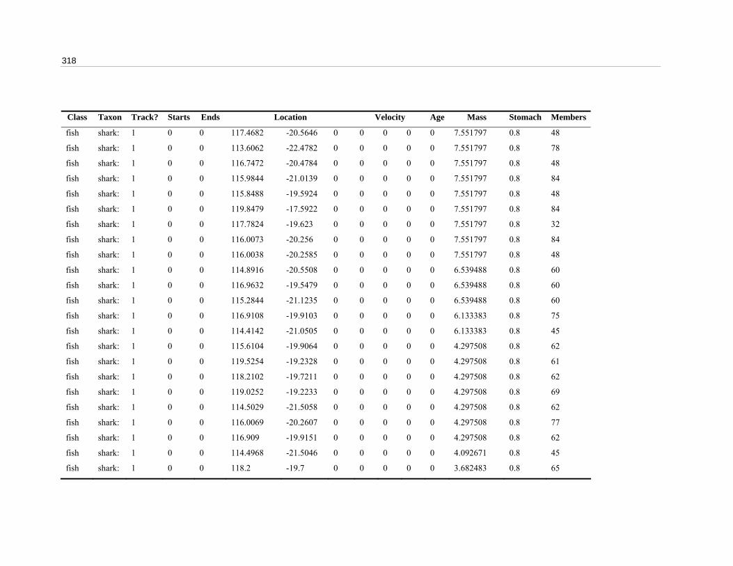
318
Class Taxon Track? Starts Ends Location Velocity Age Mass Stomach Members
fish shark: 1 0 0 117.4682 -20.5646 0 0 0 0 0 7.551797 0.8 48
fish shark: 1 0 0 113.6062 -22.4782 0 0 0 0 0 7.551797 0.8 78
fish shark: 1 0 0 116.7472 -20.4784 0 0 0 0 0 7.551797 0.8 48
fish shark: 1 0 0 115.9844 -21.0139 0 0 0 0 0 7.551797 0.8 84
fish shark: 1 0 0 115.8488 -19.5924 0 0 0 0 0 7.551797 0.8 48
fish shark: 1 0 0 119.8479 -17.5922 0 0 0 0 0 7.551797 0.8 84
fish shark: 1 0 0 117.7824 -19.623 0 0 0 0 0 7.551797 0.8 32
fish shark: 1 0 0 116.0073 -20.256 0 0 0 0 0 7.551797 0.8 84
fish shark: 1 0 0 116.0038 -20.2585 0 0 0 0 0 7.551797 0.8 48
fish shark: 1 0 0 114.8916 -20.5508 0 0 0 0 0 6.539488 0.8 60
fish shark: 1 0 0 116.9632 -19.5479 0 0 0 0 0 6.539488 0.8 60
fish shark: 1 0 0 115.2844 -21.1235 0 0 0 0 0 6.539488 0.8 60
fish shark: 1 0 0 116.9108 -19.9103 0 0 0 0 0 6.133383 0.8 75
fish shark: 1 0 0 114.4142 -21.0505 0 0 0 0 0 6.133383 0.8 45
fish shark: 1 0 0 115.6104 -19.9064 0 0 0 0 0 4.297508 0.8 62
fish shark: 1 0 0 119.5254 -19.2328 0 0 0 0 0 4.297508 0.8 61
fish shark: 1 0 0 118.2102 -19.7211 0 0 0 0 0 4.297508 0.8 62
fish shark: 1 0 0 119.0252 -19.2233 0 0 0 0 0 4.297508 0.8 69
fish shark: 1 0 0 114.5029 -21.5058 0 0 0 0 0 4.297508 0.8 62
fish shark: 1 0 0 116.0069 -20.2607 0 0 0 0 0 4.297508 0.8 77
fish shark: 1 0 0 116.909 -19.9151 0 0 0 0 0 4.297508 0.8 62
fish shark: 1 0 0 114.4968 -21.5046 0 0 0 0 0 4.092671 0.8 45
fish shark: 1 0 0 118.2 -19.7 0 0 0 0 0 3.682483 0.8 65
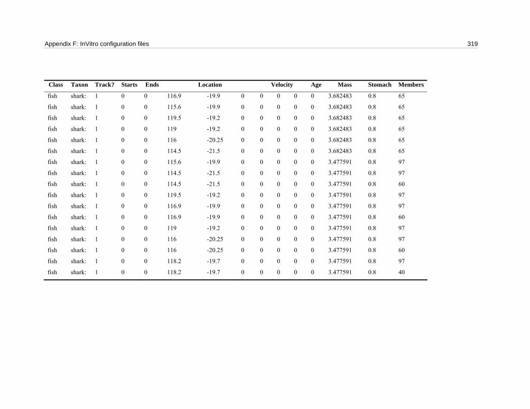
Appendix F: InVitro configuration files 319
Class Taxon Track? Starts Ends Location Velocity Age Mass Stomach Members
fish shark: 1 0 0 116.9 -19.9 0 0 0 0 0 3.682483 0.8 65
fish shark: 1 0 0 115.6 -19.9 0 0 0 0 0 3.682483 0.8 65
fish shark: 1 0 0 119.5 -19.2 0 0 0 0 0 3.682483 0.8 65
fish shark: 1 0 0 119 -19.2 0 0 0 0 0 3.682483 0.8 65
fish shark: 1 0 0 116 -20.25 0 0 0 0 0 3.682483 0.8 65
fish shark: 1 0 0 114.5 -21.5 0 0 0 0 0 3.682483 0.8 65
fish shark: 1 0 0 115.6 -19.9 0 0 0 0 0 3.477591 0.8 97
fish shark: 1 0 0 114.5 -21.5 0 0 0 0 0 3.477591 0.8 97
fish shark: 1 0 0 114.5 -21.5 0 0 0 0 0 3.477591 0.8 60
fish shark: 1 0 0 119.5 -19.2 0 0 0 0 0 3.477591 0.8 97
fish shark: 1 0 0 116.9 -19.9 0 0 0 0 0 3.477591 0.8 97
fish shark: 1 0 0 116.9 -19.9 0 0 0 0 0 3.477591 0.8 60
fish shark: 1 0 0 119 -19.2 0 0 0 0 0 3.477591 0.8 97
fish shark: 1 0 0 116 -20.25 0 0 0 0 0 3.477591 0.8 97
fish shark: 1 0 0 116 -20.25 0 0 0 0 0 3.477591 0.8 60
fish shark: 1 0 0 118.2 -19.7 0 0 0 0 0 3.477591 0.8 97
fish shark: 1 0 0 118.2 -19.7 0 0 0 0 0 3.477591 0.8 40
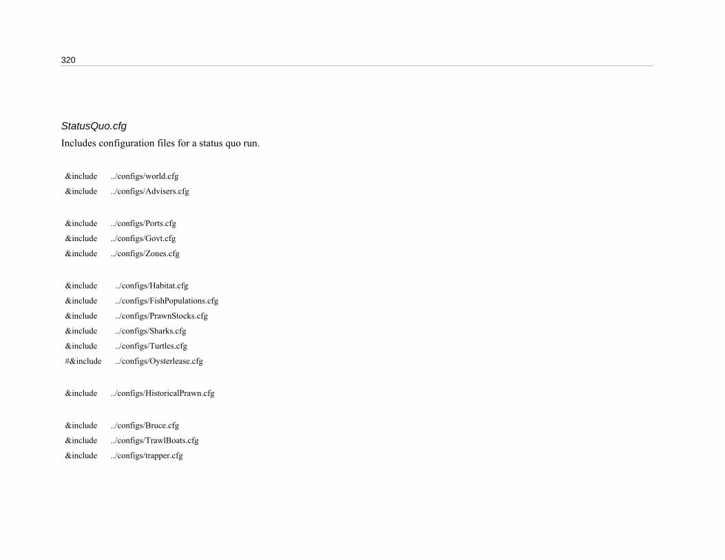
320
StatusQuo.cfg Includes configuration files for a status quo run.
&include ../configs/world.cfg
&include ../configs/Advisers.cfg
&include ../configs/Ports.cfg
&include ../configs/Govt.cfg
&include ../configs/Zones.cfg
&include ../configs/Habitat.cfg
&include ../configs/FishPopulations.cfg
&include ../configs/PrawnStocks.cfg
&include ../configs/Sharks.cfg
&include ../configs/Turtles.cfg
#&include ../configs/Oysterlease.cfg
&include ../configs/HistoricalPrawn.cfg
&include ../configs/Bruce.cfg
&include ../configs/TrawlBoats.cfg
&include ../configs/trapper.cfg

Appendix F: InVitro configuration files 321
&include ../configs/PrawnFleet.cfg
&include ../configs/Vessels.cfg
&include ../configs/Rigs.cfg
Class Taxon Track? Presence data Projection DB Projection Starts Ends
polyorganism ponyfish: 0 bycatch.xy.pt map.rc none 0 0
StatusQuo_1p.cfg Includes configuration files for a status quo run with one development pulse.
&include ../configs/world.cfg
&include ../configs/Advisers.cfg
&include ../configs/Ports_1p.cfg
&include ../configs/Govt.cfg
&include ../configs/Zones.cfg
&include ../configs/Bruce.cfg
#&include ../configs/TrawlBoats_1p.cfg
#&include ../configs/trapper.cfg

322
#&include ../configs/PrawnFleet_1p.cfg
#&include ../configs/HistoricalPrawn.cfg
&include ../configs/Vessels_1p.cfg
&include ../configs/Rigs.cfg
#&include ../configs/Habitat.cfg
#&include ../configs/FishPopulations.cfg
#&include ../configs/PrawnStocks.cfg
#&include ../configs/Sharks.cfg
#&include ../configs/Turtles.cfg
#&include ../configs/Oysterlease.cfg
StatusQuo_2p.cfg Includes configuration files for a status quo run with two development pulses.
&include ../configs/world.cfg
&include ../configs/Advisers.cfg
&include ../configs/Ports_2p.cfg
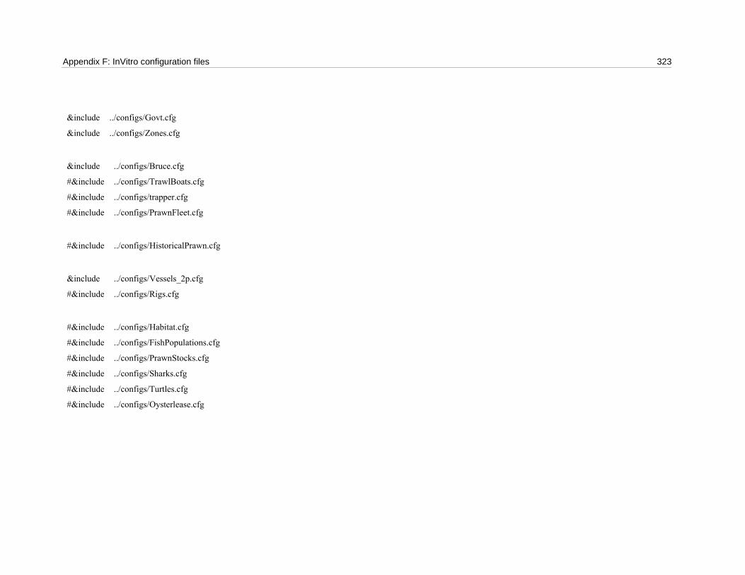
Appendix F: InVitro configuration files 323
&include ../configs/Govt.cfg
&include ../configs/Zones.cfg
&include ../configs/Bruce.cfg
#&include ../configs/TrawlBoats.cfg
#&include ../configs/trapper.cfg
#&include ../configs/PrawnFleet.cfg
#&include ../configs/HistoricalPrawn.cfg
&include ../configs/Vessels_2p.cfg
#&include ../configs/Rigs.cfg
#&include ../configs/Habitat.cfg
#&include ../configs/FishPopulations.cfg
#&include ../configs/PrawnStocks.cfg
#&include ../configs/Sharks.cfg
#&include ../configs/Turtles.cfg
#&include ../configs/Oysterlease.cfg
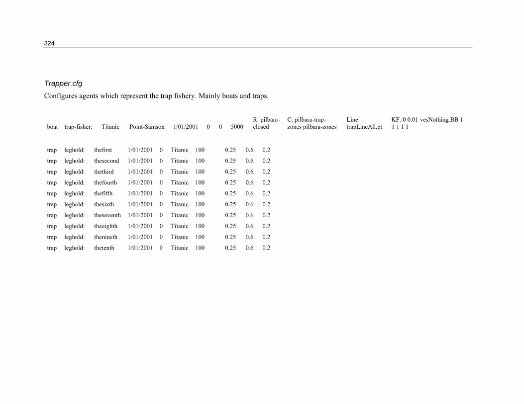
324
Trapper.cfg Configures agents which represent the trap fishery. Mainly boats and traps.
boat trap-fisher: Titanic Point-Samson 1/01/2001 0 0 5000 R: pilbara-closed
C: pilbara-trap-zones pilbara-zones
Line: trapLineAll.pt
KF: 0 0.01 vesNothing.BB 1 1 1 1 1
trap leghold: thefirst 1/01/2001 0 Titanic 100 0.25 0.6 0.2
trap leghold: thesecond 1/01/2001 0 Titanic 100 0.25 0.6 0.2
trap leghold: thethird 1/01/2001 0 Titanic 100 0.25 0.6 0.2
trap leghold: thefourth 1/01/2001 0 Titanic 100 0.25 0.6 0.2
trap leghold: thefifth 1/01/2001 0 Titanic 100 0.25 0.6 0.2
trap leghold: thesixth 1/01/2001 0 Titanic 100 0.25 0.6 0.2
trap leghold: theseventh 1/01/2001 0 Titanic 100 0.25 0.6 0.2
trap leghold: theeighth 1/01/2001 0 Titanic 100 0.25 0.6 0.2
trap leghold: thenineth 1/01/2001 0 Titanic 100 0.25 0.6 0.2
trap leghold: thetenth 1/01/2001 0 Titanic 100 0.25 0.6 0.2
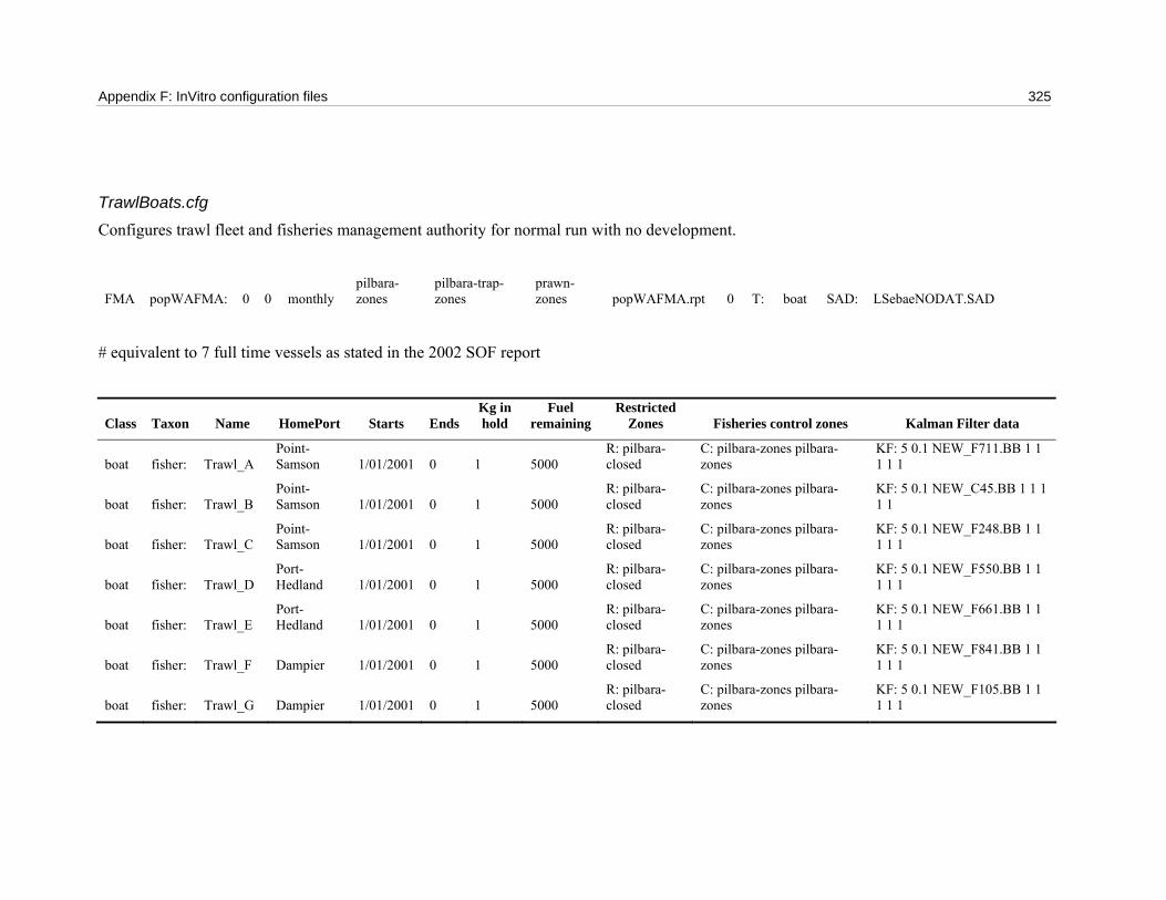
Appendix F: InVitro configuration files 325
TrawlBoats.cfg Configures trawl fleet and fisheries management authority for normal run with no development.
FMA popWAFMA: 0 0 monthly pilbara-zones
pilbara-trap-zones
prawn-zones popWAFMA.rpt 0 T: boat SAD: LSebaeNODAT.SAD
# equivalent to 7 full time vessels as stated in the 2002 SOF report
Class Taxon Name HomePort Starts Ends Kg in hold
Fuel remaining
Restricted Zones Fisheries control zones Kalman Filter data
boat fisher: Trawl_A Point-Samson 1/01/2001 0 1 5000
R: pilbara-closed
C: pilbara-zones pilbara-zones
KF: 5 0.1 NEW_F711.BB 1 1 1 1 1
boat fisher: Trawl_B Point-Samson 1/01/2001 0 1 5000
R: pilbara-closed
C: pilbara-zones pilbara-zones
KF: 5 0.1 NEW_C45.BB 1 1 1 1 1
boat fisher: Trawl_C Point-Samson 1/01/2001 0 1 5000
R: pilbara-closed
C: pilbara-zones pilbara-zones
KF: 5 0.1 NEW_F248.BB 1 1 1 1 1
boat fisher: Trawl_D Port-Hedland 1/01/2001 0 1 5000
R: pilbara-closed
C: pilbara-zones pilbara-zones
KF: 5 0.1 NEW_F550.BB 1 1 1 1 1
boat fisher: Trawl_E Port-Hedland 1/01/2001 0 1 5000
R: pilbara-closed
C: pilbara-zones pilbara-zones
KF: 5 0.1 NEW_F661.BB 1 1 1 1 1
boat fisher: Trawl_F Dampier 1/01/2001 0 1 5000 R: pilbara-closed
C: pilbara-zones pilbara-zones
KF: 5 0.1 NEW_F841.BB 1 1 1 1 1
boat fisher: Trawl_G Dampier 1/01/2001 0 1 5000 R: pilbara-closed
C: pilbara-zones pilbara-zones
KF: 5 0.1 NEW_F105.BB 1 1 1 1 1
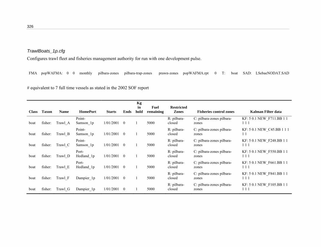
326
TrawlBoats_1p.cfg Configures trawl fleet and fisheries management authority for run with one development pulse.
FMA popWAFMA: 0 0 monthly pilbara-zones pilbara-trap-zones prawn-zones popWAFMA.rpt 0 T: boat SAD: LSebaeNODAT.SAD
# equivalent to 7 full time vessels as stated in the 2002 SOF report
Class Taxon Name HomePort Starts Ends
Kg in
hold Fuel
remaining Restricted
Zones Fisheries control zones Kalman Filter data
boat fisher: Trawl_A Point-Samson_1p 1/01/2001 0 1 5000
R: pilbara-closed
C: pilbara-zones pilbara-zones
KF: 5 0.1 NEW_F711.BB 1 1 1 1 1
boat fisher: Trawl_B Point-Samson_1p 1/01/2001 0 1 5000
R: pilbara-closed
C: pilbara-zones pilbara-zones
KF: 5 0.1 NEW_C45.BB 1 1 1 1 1
boat fisher: Trawl_C Point-Samson_1p 1/01/2001 0 1 5000
R: pilbara-closed
C: pilbara-zones pilbara-zones
KF: 5 0.1 NEW_F248.BB 1 1 1 1 1
boat fisher: Trawl_D Port-Hedland_1p 1/01/2001 0 1 5000
R: pilbara-closed
C: pilbara-zones pilbara-zones
KF: 5 0.1 NEW_F550.BB 1 1 1 1 1
boat fisher: Trawl_E Port-Hedland_1p 1/01/2001 0 1 5000
R: pilbara-closed
C: pilbara-zones pilbara-zones
KF: 5 0.1 NEW_F661.BB 1 1 1 1 1
boat fisher: Trawl_F Dampier_1p 1/01/2001 0 1 5000 R: pilbara-closed
C: pilbara-zones pilbara-zones
KF: 5 0.1 NEW_F841.BB 1 1 1 1 1
boat fisher: Trawl_G Dampier_1p 1/01/2001 0 1 5000 R: pilbara-closed
C: pilbara-zones pilbara-zones
KF: 5 0.1 NEW_F105.BB 1 1 1 1 1

Appendix F: InVitro configuration files 327
Turtles.cfg Configures the agents which represent the turtle population.
Class Taxon Starts Ends Sample interval Report file Target type Include blastula Only recruits Targets
biomass turtleesky: 0 0 monthly turtle_bio.tbl 1 0 0 turtle
Class Taxon Starts Ends Sample interval Report file Target type
tracker turtles: 0 0 monthly turtlemap turtle
Class Taxon Track? Starts Ends Location Velocity Age Mass
blastula turtle: 1 0 0 115.4 -21 0 0 0 0 0
blastula turtle: 1 0 0 115.5 -20.4 0 0 0 0 0
blastula turtle: 1 0 0 118 -20.3 0 0 0 0 0
blastula turtle: 1 0 0 115.5 -20.4 0 0 0 0 0
blastula turtle: 1 0 0 114.3 -21.75 0 0 0 0 0
blastula turtle: 1 0 0 116.6 -20.45 0 0 0 0 0
blastula turtle: 1 0 0 115.6 -20.6 0 0 0 0 0

328
Class Taxon Track? Starts Ends Location Velocity Age Mass Stomach Members
fish turtle: 0 0 0 119.626 -18.3408 0 0 0 0 0 77.373718 0.8 30
fish turtle: 0 0 0 117.6453 -20.5794 0 0 0 0 0 60.449303 0.8 39
fish turtle: 0 0 0 118.3991 -19.0293 0 0 0 0 0 69.318794 0.8 48
fish turtle: 0 0 0 117.1682 -19.2809 0 0 0 0 0 64.598717 0.8 57
fish turtle: 0 0 0 116.6878 -20.047 0 0 0 0 0 74.559196 0.8 51
fish turtle: 0 0 0 115.5264 -20.3564 0 0 0 0 0 62.225616 0.8 36
fish turtle: 0 0 0 116.5319 -20.3589 0 0 0 0 0 62.51004 0.8 33
fish turtle: 0 0 0 115.3349 -21.3375 0 0 0 0 0 67.897362 0.8 28
fish turtle: 0 0 0 119.7569 -18.8276 0 0 0 0 0 73.411179 0.8 28
fish turtle: 0 0 0 115.2862 -20.4456 0 0 0 0 0 71.370979 0.8 57
fish turtle: 0 0 0 118.7833 -20.0467 0 0 0 0 0 66.722237 0.8 42
fish turtle: 0 0 0 119.5561 -19.5824 0 0 0 0 0 55.089573 0.8 72
fish turtle: 0 0 0 118.7179 -19.9394 0 0 0 0 0 72.745392 0.8 60
fish turtle: 0 0 0 119.8248 -17.7526 0 0 0 0 0 68.58651 0.8 42
fish turtle: 0 0 0 117.7617 -20.5348 0 0 0 0 0 59.111237 0.8 66
fish turtle: 0 0 0 119.91 -18.2863 0 0 0 0 0 72.207169 0.8 75
fish turtle: 0 0 0 119.71 -17.2244 0 0 0 0 0 59.876133 0.8 54
fish turtle: 0 0 0 115.7077 -19.7782 0 0 0 0 0 76.158577 0.8 33
fish turtle: 0 0 0 119.3087 -19.8402 0 0 0 0 0 51.254185 0.8 78
fish turtle: 0 0 0 119.6949 -19.7413 0 0 0 0 0 75.361786 0.8 24
fish turtle: 0 0 0 118.1109 -19.5315 0 0 0 0 0 54.52739 0.8 49

Appendix F: InVitro configuration files 329
Class Taxon Track? Starts Ends Location Velocity Age Mass Stomach Members
fish turtle: 0 0 0 115.6928 -20.1673 0 0 0 0 0 60.449303 0.8 45
fish turtle: 0 0 0 119.2525 -18.1397 0 0 0 0 0 76.986641 0.8 42
fish turtle: 0 0 0 118.1011 -19.8719 0 0 0 0 0 67.818466 0.8 27
fish turtle: 0 0 0 118.9684 -19.5825 0 0 0 0 0 64.598717 0.8 29
fish turtle: 0 0 0 119.2097 -19.1555 0 0 0 0 0 62.225616 0.8 56
fish turtle: 0 0 0 119.4109 -19.8014 0 0 0 0 0 67.897362 0.8 33
fish turtle: 0 0 0 116.9994 -20.6013 0 0 0 0 0 57.465912 0.8 48
fish turtle: 0 0 0 119.7846 -19.8225 0 0 0 0 0 66.722237 0.8 72
fish turtle: 0 0 0 119.7218 -19.4813 0 0 0 0 0 70.454063 0.8 48
fish turtle: 0 0 0 119.5833 -18.427 0 0 0 0 0 71.117302 0.8 45
fish turtle: 0 0 0 119.6101 -19.7884 0 0 0 0 0 64.170471 0.8 36
fish turtle: 0 0 0 118.8591 -17.7155 0 0 0 0 0 54.64436 0.8 43
fish turtle: 0 0 0 117.12 -19.7349 0 0 0 0 0 80.5 0.8 63
fish turtle: 0 0 0 119.3437 -19.2151 0 0 0 0 0 80.9 0.8 84
fish turtle: 0 0 0 119.4748 -18.5837 0 0 0 0 0 81.8 0.8 72
fish turtle: 0 0 0 119.3687 -19.5884 0 0 0 0 0 81.56 0.8 33
fish turtle: 0 0 0 119.8745 -17.7149 0 0 0 0 0 82.88 0.8 87
fish turtle: 0 0 0 119.4416 -19.4521 0 0 0 0 0 82.59 0.8 36
fish turtle: 0 0 0 118.0842 -19.6769 0 0 0 0 0 47.58 0.8 75
fish turtle: 0 0 0 116.5331 -19.7409 0 0 0 0 0 47.68 0.8 78
fish turtle: 0 0 0 115.5078 -20.4422 0 0 0 0 0 47.69 0.8 63
fish turtle: 0 0 0 119.5749 -19.8616 0 0 0 0 0 47.6 0.8 78
fish turtle: 0 0 0 119.5138 -18.2478 0 0 0 0 0 47.9 0.8 63

330
Class Taxon Track? Starts Ends Location Velocity Age Mass Stomach Members
fish turtle: 0 0 0 118.6171 -19.1976 0 0 0 0 0 47.82 0.8 57
fish turtle: 0 0 0 119.2912 -19.4755 0 0 0 0 0 47.1 0.8 78
fish turtle: 0 0 0 118.4534 -19.586 0 0 0 0 0 47.3 0.8 72
fish turtle: 0 0 0 118.4802 -18.0028 0 0 0 0 0 47.22 0.8 75
fish turtle: 0 0 0 119.3372 -19.4749 0 0 0 0 0 47.17 0.8 82
fish turtle: 0 0 0 119.9627 -18.9181 0 0 0 0 0 47.99 0.8 75
fish turtle: 0 0 0 119.6988 -19.5093 0 0 0 0 0 47.51 0.8 66
fish turtle: 0 0 0 117.2118 -18.713 0 0 0 0 0 47.43 0.8 78
fish turtle: 0 0 0 117.0192 -20.521 0 0 0 0 0 47.78 0.8 75
fish turtle: 0 0 0 114.217 -21.5308 0 0 0 0 0 83.71 0.8 56
fish turtle: 0 0 0 115.8824 -20.7013 0 0 0 0 0 83.79 0.8 72
fish turtle: 0 0 0 118.9903 -17.8816 0 0 0 0 0 84.73 0.8 48
fish turtle: 0 0 0 116.9083 -19.1776 0 0 0 0 0 84.7 0.8 48
fish turtle: 0 0 0 118.7941 -18.0901 0 0 0 0 0 45.75 0.8 33
fish turtle: 0 0 0 114.2091 -21.9235 0 0 0 0 0 45.91 0.8 99
fish turtle: 0 0 0 117.2031 -19.1955 0 0 0 0 0 45.1 0.8 44
fish turtle: 0 0 0 115.7037 -19.4642 0 0 0 0 0 45.13 0.8 63
fish turtle: 0 0 0 115.4879 -20.6262 0 0 0 0 0 45.19 0.8 72
fish turtle: 0 0 0 119.8872 -17.7442 0 0 0 0 0 45.03 0.8 36
fish turtle: 0 0 0 114.8118 -20.5805 0 0 0 0 0 45.09 0.8 66
fish turtle: 0 0 0 114.3091 -22.1919 0 0 0 0 0 45.97 0.8 87
fish turtle: 0 0 0 119.5615 -19.3442 0 0 0 0 0 45.91 0.8 72
fish turtle: 0 0 0 117.9185 -18.5186 0 0 0 0 0 45.93 0.8 90

Appendix F: InVitro configuration files 331
Class Taxon Track? Starts Ends Location Velocity Age Mass Stomach Members
fish turtle: 0 0 0 118.5412 -18.3213 0 0 0 0 0 45.45 0.8 74
fish turtle: 0 0 0 116.5969 -19.4525 0 0 0 0 0 45.62 0.8 99
fish turtle: 0 0 0 117.979 -18.7888 0 0 0 0 0 45.94 0.8 72
fish turtle: 0 0 0 119.5946 -18.8403 0 0 0 0 0 45.21 0.8 93
fish turtle: 0 0 0 119.9001 -19.6549 0 0 0 0 0 45.34 0.8 73
fish turtle: 0 0 0 118.5713 -20.1284 0 0 0 0 0 85.78595 0.8 78
fish turtle: 0 0 0 118.4379 -18.827 0 0 0 0 0 85.78595 0.8 99
fish turtle: 0 0 0 119.9705 -17.6217 0 0 0 0 0 86.78595 0.8 27
fish turtle: 0 0 0 119.5605 -19.8156 0 0 0 0 0 86.78595 0.8 90
fish turtle: 0 0 0 118.7944 -18.8991 0 0 0 0 0 87.78595 0.8 75
fish turtle: 0 0 0 116.1555 -19.2854 0 0 0 0 0 87.78595 0.8 26
fish turtle: 0 0 0 118.592 -19.8358 0 0 0 0 0 43.78595 0.8 80
fish turtle: 0 0 0 115.9544 -20.5845 0 0 0 0 0 43.78595 0.8 66
fish turtle: 0 0 0 118.5179 -19.6685 0 0 0 0 0 43.78595 0.8 65
fish turtle: 0 0 0 119.536 -18.2607 0 0 0 0 0 43.78595 0.8 60
fish turtle: 0 0 0 119.3247 -19.1898 0 0 0 0 0 43.78595 0.8 57
fish turtle: 0 0 0 116.1383 -19.1431 0 0 0 0 0 43.78595 0.8 63
fish turtle: 0 0 0 118.4504 -20.1998 0 0 0 0 0 43.78595 0.8 66
fish turtle: 0 0 0 119.2679 -18.3855 0 0 0 0 0 43.78595 0.8 27
fish turtle: 0 0 0 115.4651 -21.1667 0 0 0 0 0 43.78595 0.8 75
fish turtle: 0 0 0 114.4099 -21.947 0 0 0 0 0 43.78595 0.8 90
fish turtle: 0 0 0 119.8194 -18.5009 0 0 0 0 0 88.79335 0.8 67
fish turtle: 0 0 0 117.9359 -19.1948 0 0 0 0 0 88.79335 0.8 96

332
Class Taxon Track? Starts Ends Location Velocity Age Mass Stomach Members
fish turtle: 0 0 0 117.7386 -19.392 0 0 0 0 0 89.79335 0.8 75
fish turtle: 0 0 0 119.2582 -19.6599 0 0 0 0 0 89.79335 0.8 33
fish turtle: 0 0 0 119.8178 -19.2181 0 0 0 0 0 90.79335 0.8 74
fish turtle: 0 0 0 119.5596 -17.4348 0 0 0 0 0 90.79335 0.8 25
fish turtle: 0 0 0 115.6964 -21.0028 0 0 0 0 0 41.79335 0.8 78
fish turtle: 0 0 0 118.9671 -19.7084 0 0 0 0 0 41.79335 0.8 90
fish turtle: 0 0 0 116.6052 -20.5268 0 0 0 0 0 41.79335 0.8 102
fish turtle: 0 0 0 119.2677 -19.6768 0 0 0 0 0 41.79335 0.8 105
fish turtle: 0 0 0 115.2586 -21.2397 0 0 0 0 0 41.79335 0.8 66
fish turtle: 0 0 0 119.1275 -17.4474 0 0 0 0 0 41.79335 0.8 29
fish turtle: 0 0 0 119.8746 -17.7971 0 0 0 0 0 41.79335 0.8 99
fish turtle: 0 0 0 118.5803 -18.4509 0 0 0 0 0 41.79335 0.8 73
fish turtle: 0 0 0 117.6858 -20.2878 0 0 0 0 0 41.79335 0.8 74
fish turtle: 0 0 0 115.8336 -21.0363 0 0 0 0 0 91.730122 0.8 101
fish turtle: 0 0 0 115.0901 -20.4574 0 0 0 0 0 91.730122 0.8 100
fish turtle: 0 0 0 118.5981 -17.8672 0 0 0 0 0 47.730122 0.8 60
fish turtle: 0 0 0 115.8294 -20.3563 0 0 0 0 0 47.730122 0.8 71
fish turtle: 0 0 0 115.6418 -19.8654 0 0 0 0 0 47.730122 0.8 79
fish turtle: 0 0 0 114.3599 -21.8103 0 0 0 0 0 39.730122 0.8 70
fish turtle: 0 0 0 119.5917 -18.3214 0 0 0 0 0 39.730122 0.8 60
fish turtle: 0 0 0 118.7747 -18.4145 0 0 0 0 0 39.730122 0.8 90
fish turtle: 0 0 0 117.0332 -19.3279 0 0 0 0 0 39.730122 0.8 93
fish turtle: 0 0 0 114.105 -22.0902 0 0 0 0 0 39.730122 0.8 93

Appendix F: InVitro configuration files 333
Class Taxon Track? Starts Ends Location Velocity Age Mass Stomach Members
fish turtle: 0 0 0 119.6341 -19.688 0 0 0 0 0 39.730122 0.8 93
fish turtle: 0 0 0 118.9752 -17.4564 0 0 0 0 0 39.730122 0.8 104
fish turtle: 0 0 0 117.3208 -18.6784 0 0 0 0 0 39.730122 0.8 63
fish turtle: 0 0 0 119.7186 -17.5088 0 0 0 0 0 39.730122 0.8 55
fish turtle: 0 0 0 115.0509 -20.8063 0 0 0 0 0 39.730122 0.8 63
fish turtle: 0 0 0 119.8945 -19.5357 0 0 0 0 0 39.730122 0.8 44
fish turtle: 0 0 0 115.9956 -20.5191 0 0 0 0 0 39.730122 0.8 63
fish turtle: 0 0 0 116.5091 -18.849 0 0 0 0 0 39.730122 0.8 62
fish turtle: 0 0 0 114.1024 -21.5328 0 0 0 0 0 39.730122 0.8 90
fish turtle: 0 0 0 119.0164 -19.0093 0 0 0 0 0 45.5937 0.8 75
fish turtle: 0 0 0 119.6019 -19.8966 0 0 0 0 0 45.5937 0.8 61
fish turtle: 0 0 0 118.9088 -18.9141 0 0 0 0 0 45.5937 0.8 105
fish turtle: 0 0 0 119.7473 -18.0385 0 0 0 0 0 37.5937 0.8 76
fish turtle: 0 0 0 119.8572 -18.1181 0 0 0 0 0 37.5937 0.8 118
fish turtle: 0 0 0 119.5977 -19.7792 0 0 0 0 0 37.5937 0.8 91
fish turtle: 0 0 0 119.5081 -19.8303 0 0 0 0 0 37.5937 0.8 74
fish turtle: 0 0 0 119.0344 -19.7451 0 0 0 0 0 37.5937 0.8 96
fish turtle: 0 0 0 117.8531 -19.156 0 0 0 0 0 37.5937 0.8 74
fish turtle: 0 0 0 114.3927 -21.6766 0 0 0 0 0 37.5937 0.8 98
fish turtle: 0 0 0 118.5497 -19.9828 0 0 0 0 0 37.5937 0.8 76
fish turtle: 0 0 0 119.5486 -19.6775 0 0 0 0 0 37.5937 0.8 61
fish turtle: 0 0 0 116.9409 -19.7338 0 0 0 0 0 37.5937 0.8 91
fish turtle: 0 0 0 119.0948 -19.6405 0 0 0 0 0 37.5937 0.8 107
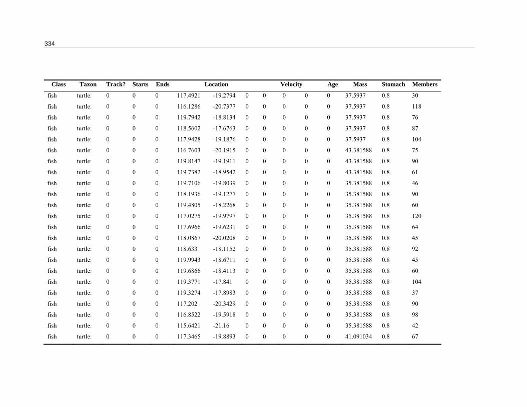
334
Class Taxon Track? Starts Ends Location Velocity Age Mass Stomach Members
fish turtle: 0 0 0 117.4921 -19.2794 0 0 0 0 0 37.5937 0.8 30
fish turtle: 0 0 0 116.1286 -20.7377 0 0 0 0 0 37.5937 0.8 118
fish turtle: 0 0 0 119.7942 -18.8134 0 0 0 0 0 37.5937 0.8 76
fish turtle: 0 0 0 118.5602 -17.6763 0 0 0 0 0 37.5937 0.8 87
fish turtle: 0 0 0 117.9428 -19.1876 0 0 0 0 0 37.5937 0.8 104
fish turtle: 0 0 0 116.7603 -20.1915 0 0 0 0 0 43.381588 0.8 75
fish turtle: 0 0 0 119.8147 -19.1911 0 0 0 0 0 43.381588 0.8 90
fish turtle: 0 0 0 119.7382 -18.9542 0 0 0 0 0 43.381588 0.8 61
fish turtle: 0 0 0 119.7106 -19.8039 0 0 0 0 0 35.381588 0.8 46
fish turtle: 0 0 0 118.1936 -19.1277 0 0 0 0 0 35.381588 0.8 90
fish turtle: 0 0 0 119.4805 -18.2268 0 0 0 0 0 35.381588 0.8 60
fish turtle: 0 0 0 117.0275 -19.9797 0 0 0 0 0 35.381588 0.8 120
fish turtle: 0 0 0 117.6966 -19.6231 0 0 0 0 0 35.381588 0.8 64
fish turtle: 0 0 0 118.0867 -20.0208 0 0 0 0 0 35.381588 0.8 45
fish turtle: 0 0 0 118.633 -18.1152 0 0 0 0 0 35.381588 0.8 92
fish turtle: 0 0 0 119.9943 -18.6711 0 0 0 0 0 35.381588 0.8 45
fish turtle: 0 0 0 119.6866 -18.4113 0 0 0 0 0 35.381588 0.8 60
fish turtle: 0 0 0 119.3771 -17.841 0 0 0 0 0 35.381588 0.8 104
fish turtle: 0 0 0 119.3274 -17.8983 0 0 0 0 0 35.381588 0.8 37
fish turtle: 0 0 0 117.202 -20.3429 0 0 0 0 0 35.381588 0.8 90
fish turtle: 0 0 0 116.8522 -19.5918 0 0 0 0 0 35.381588 0.8 98
fish turtle: 0 0 0 115.6421 -21.16 0 0 0 0 0 35.381588 0.8 42
fish turtle: 0 0 0 117.3465 -19.8893 0 0 0 0 0 41.091034 0.8 67

Appendix F: InVitro configuration files 335
Class Taxon Track? Starts Ends Location Velocity Age Mass Stomach Members
fish turtle: 0 0 0 119.1889 -18.0552 0 0 0 0 0 41.091034 0.8 47
fish turtle: 0 0 0 119.3496 -19.2459 0 0 0 0 0 41.091034 0.8 94
fish turtle: 0 0 0 119.4407 -17.6911 0 0 0 0 0 33.091034 0.8 90
fish turtle: 0 0 0 116.6232 -19.7321 0 0 0 0 0 33.091034 0.8 77
fish turtle: 0 0 0 119.1693 -18.6676 0 0 0 0 0 33.091034 0.8 120
fish turtle: 0 0 0 119.5396 -18.4785 0 0 0 0 0 33.091034 0.8 28
fish turtle: 0 0 0 118.6974 -19.2398 0 0 0 0 0 33.091034 0.8 76
fish turtle: 0 0 0 117.9379 -20.1353 0 0 0 0 0 33.091034 0.8 31
fish turtle: 0 0 0 119.7369 -17.2698 0 0 0 0 0 33.091034 0.8 92
fish turtle: 0 0 0 119.7682 -18.2476 0 0 0 0 0 33.091034 0.8 37
fish turtle: 0 0 0 116.5881 -20.0066 0 0 0 0 0 33.091034 0.8 82
fish turtle: 0 0 0 115.6055 -19.9109 0 0 0 0 0 33.091034 0.8 47
fish turtle: 0 0 0 116.7853 -20.3865 0 0 0 0 0 33.091034 0.8 42
fish turtle: 0 0 0 117.1503 -20.5552 0 0 0 0 0 39.719305 0.8 104
fish turtle: 0 0 0 119.7454 -19.6801 0 0 0 0 0 39.719305 0.8 108
fish turtle: 0 0 0 115.3208 -21.139 0 0 0 0 0 37.719305 0.8 90
fish turtle: 0 0 0 119.5091 -19.427 0 0 0 0 0 37.719305 0.8 99
fish turtle: 0 0 0 118.7896 -19.2235 0 0 0 0 0 30.719305 0.8 46
fish turtle: 0 0 0 119.3756 -18.981 0 0 0 0 0 30.719305 0.8 120
fish turtle: 0 0 0 115.8626 -20.204 0 0 0 0 0 30.719305 0.8 108
fish turtle: 0 0 0 116.3874 -20.2267 0 0 0 0 0 30.719305 0.8 105
fish turtle: 0 0 0 117.9956 -19.5447 0 0 0 0 0 30.719305 0.8 104
fish turtle: 0 0 0 119.8574 -17.9975 0 0 0 0 0 30.719305 0.8 105
336
Class Taxon Track? Starts Ends Location Velocity Age Mass Stomach Members
fish turtle: 0 0 0 119.645 -19.7066 0 0 0 0 0 30.719305 0.8 103
fish turtle: 0 0 0 119.4659 -19.475 0 0 0 0 0 30.719305 0.8 102
fish turtle: 0 0 0 118.6909 -17.7415 0 0 0 0 0 30.719305 0.8 40
fish turtle: 0 0 0 119.7927 -18.8021 0 0 0 0 0 30.719305 0.8 102
fish turtle: 0 0 0 114.5936 -21.5366 0 0 0 0 0 30.719305 0.8 46
fish turtle: 0 0 0 115.5087 -21.2839 0 0 0 0 0 35.2635 0.8 79
fish turtle: 0 0 0 119.7827 -19.2139 0 0 0 0 0 35.2635 0.8 109
fish turtle: 0 0 0 116.2878 -19.8021 0 0 0 0 0 33.2635 0.8 61
fish turtle: 0 0 0 115.8827 -20.8845 0 0 0 0 0 33.2635 0.8 108
fish turtle: 0 0 0 118.9303 -19.3337 0 0 0 0 0 28.2635 0.8 60
fish turtle: 0 0 0 118.7624 -19.4249 0 0 0 0 0 28.2635 0.8 106
fish turtle: 0 0 0 119.4233 -19.008 0 0 0 0 0 28.2635 0.8 60
fish turtle: 0 0 0 114.8635 -20.7258 0 0 0 0 0 28.2635 0.8 92
fish turtle: 0 0 0 119.6285 -19.8341 0 0 0 0 0 28.2635 0.8 42
fish turtle: 0 0 0 119.768 -18.8045 0 0 0 0 0 28.2635 0.8 102
fish turtle: 0 0 0 118.4293 -19.6369 0 0 0 0 0 28.2635 0.8 78
fish turtle: 0 0 0 119.779 -17.3447 0 0 0 0 0 28.2635 0.8 94
fish turtle: 0 0 0 119.9144 -18.5419 0 0 0 0 0 28.2635 0.8 62
fish turtle: 0 0 0 118.5272 -17.7558 0 0 0 0 0 30.720646 0.8 94
fish turtle: 0 0 0 116.1058 -19.789 0 0 0 0 0 30.720646 0.8 37
fish turtle: 0 0 0 114.5234 -21.5391 0 0 0 0 0 28.720646 0.8 106
fish turtle: 0 0 0 116.7083 -19.8894 0 0 0 0 0 28.720646 0.8 44
fish turtle: 0 0 0 119.5569 -18.1045 0 0 0 0 0 25.720646 0.8 121

Appendix F: InVitro configuration files 337
Class Taxon Track? Starts Ends Location Velocity Age Mass Stomach Members
fish turtle: 0 0 0 119.5439 -18.7498 0 0 0 0 0 25.720646 0.8 62
fish turtle: 0 0 0 116.2122 -18.9665 0 0 0 0 0 25.720646 0.8 91
fish turtle: 0 0 0 115.1873 -20.1216 0 0 0 0 0 25.720646 0.8 58
fish turtle: 0 0 0 114.3518 -21.0013 0 0 0 0 0 25.720646 0.8 129
fish turtle: 0 0 0 118.5606 -17.8128 0 0 0 0 0 25.720646 0.8 46
fish turtle: 0 0 0 116.7187 -19.9501 0 0 0 0 0 25.720646 0.8 121
fish turtle: 0 0 0 118.0037 -20.18 0 0 0 0 0 25.720646 0.8 49
fish turtle: 0 0 0 116.2214 -20.044 0 0 0 0 0 25.720646 0.8 121
fish turtle: 0 0 0 115.6708 -19.7002 0 0 0 0 0 25.720646 0.8 42
fish turtle: 0 0 0 119.9786 -19.3843 0 0 0 0 0 23.087664 0.8 120
fish turtle: 0 0 0 118.8663 -19.7419 0 0 0 0 0 23.087664 0.8 36
fish turtle: 0 0 0 115.7849 -20.2663 0 0 0 0 0 23.087664 0.8 121
fish turtle: 0 0 0 114.2207 -22.0011 0 0 0 0 0 23.087664 0.8 41
fish turtle: 0 0 0 118.5749 -19.8512 0 0 0 0 0 23.087664 0.8 148
fish turtle: 0 0 0 119.6759 -19.5119 0 0 0 0 0 23.087664 0.8 42
fish turtle: 0 0 0 118.4753 -19.9604 0 0 0 0 0 23.087664 0.8 120
fish turtle: 0 0 0 119.0959 -19.4371 0 0 0 0 0 23.087664 0.8 37
fish turtle: 0 0 0 118.1838 -19.841 0 0 0 0 0 23.087664 0.8 39
fish turtle: 0 0 0 118.8421 -19.1051 0 0 0 0 0 23.087664 0.8 124
fish turtle: 0 0 0 117.5872 -19.8043 0 0 0 0 0 23.087664 0.8 37
fish turtle: 0 0 0 119.2269 -19.7005 0 0 0 0 0 23.087664 0.8 107
fish turtle: 0 0 0 119.597 -18.9571 0 0 0 0 0 23.087664 0.8 46
fish turtle: 0 0 0 116.7197 -19.7764 0 0 0 0 0 20.361341 0.8 129
338
Class Taxon Track? Starts Ends Location Velocity Age Mass Stomach Members
fish turtle: 0 0 0 118.9699 -19.8992 0 0 0 0 0 20.361341 0.8 39
fish turtle: 0 0 0 119.0529 -18.1786 0 0 0 0 0 20.361341 0.8 121
fish turtle: 0 0 0 119.1243 -19.2004 0 0 0 0 0 20.361341 0.8 30
fish turtle: 0 0 0 117.6761 -19.4055 0 0 0 0 0 20.361341 0.8 108
fish turtle: 0 0 0 119.6226 -18.8107 0 0 0 0 0 20.361341 0.8 48
fish turtle: 0 0 0 117.4514 -20.2391 0 0 0 0 0 20.361341 0.8 108
fish turtle: 0 0 0 119.0328 -18.9812 0 0 0 0 0 20.361341 0.8 47
fish turtle: 0 0 0 119.0716 -18.1833 0 0 0 0 0 20.361341 0.8 102
fish turtle: 0 0 0 119.1336 -19.1788 0 0 0 0 0 20.361341 0.8 103
fish turtle: 0 0 0 118.0503 -19.8613 0 0 0 0 0 20.361341 0.8 47
fish turtle: 0 0 0 117.8061 -20.4235 0 0 0 0 0 20.361341 0.8 121
fish turtle: 0 0 0 115.5809 -20.3684 0 0 0 0 0 20.361341 0.8 52
fish turtle: 0 0 0 118.282 -19.0518 0 0 0 0 0 18.615352 0.8 124
fish turtle: 0 0 0 119.416 -18.9778 0 0 0 0 0 18.615352 0.8 124
fish turtle: 0 0 0 116.1257 -19.9278 0 0 0 0 0 18.615352 0.8 127
fish turtle: 0 0 0 119.0776 -19.7728 0 0 0 0 0 18.615352 0.8 129
fish turtle: 0 0 0 119.3889 -19.185 0 0 0 0 0 18.615352 0.8 126
fish turtle: 0 0 0 119.9653 -18.6649 0 0 0 0 0 18.615352 0.8 122
fish turtle: 0 0 0 119.7372 -19.3527 0 0 0 0 0 18.615352 0.8 56
fish turtle: 0 0 0 119.3843 -19.73 0 0 0 0 0 18.588714 0.8 124
fish turtle: 0 0 0 119.4901 -19.6115 0 0 0 0 0 18.588714 0.8 122
fish turtle: 0 0 0 119.7123 -19.4612 0 0 0 0 0 18.588714 0.8 129
fish turtle: 0 0 0 118.1509 -19.584 0 0 0 0 0 18.588714 0.8 124

Appendix F: InVitro configuration files 339
Class Taxon Track? Starts Ends Location Velocity Age Mass Stomach Members
fish turtle: 0 0 0 119.8927 -18.6256 0 0 0 0 0 18.588714 0.8 123
fish turtle: 0 0 0 119.1339 -18.1589 0 0 0 0 0 18.588714 0.8 124
fish turtle: 0 0 0 119.799 -17.4994 0 0 0 0 0 18.209777 0.8 123
fish turtle: 0 0 0 118.0058 -20.3207 0 0 0 0 0 18.209777 0.8 120
fish turtle: 0 0 0 118.159 -18.9688 0 0 0 0 0 18.209777 0.8 122
fish turtle: 0 0 0 119.6661 -18.3359 0 0 0 0 0 18.209777 0.8 122
fish turtle: 0 0 0 114.2359 -22.2251 0 0 0 0 0 18.209777 0.8 120
fish turtle: 0 0 0 114.3046 -21.7791 0 0 0 0 0 18.209777 0.8 129
fish turtle: 0 0 0 118.8784 -20.1205 0 0 0 0 0 18.209777 0.8 122
fish turtle: 0 0 0 115.6 -20.6 0 0 0 0 0 18.49739 0.8 126
fish turtle: 0 0 0 115.5 -20.4 0 0 0 0 0 18.49739 0.8 106
fish turtle: 0 0 0 118 -20.3 0 0 0 0 0 18.49739 0.8 104
fish turtle: 0 0 0 118.7419 -19.2147 0 0 0 0 0 18.49739 0.8 106
fish turtle: 0 0 0 116.6 -20.45 0 0 0 0 0 18.49739 0.8 104
fish turtle: 0 0 0 114.3 -21.75 0 0 0 0 0 18.49739 0.8 105
fish turtle: 0 0 0 115.4 -21 0 0 0 0 0 18.49739 0.8 106
340
Vessels.cfg
Class Taxon Starts Ends Sample interval Report file Targets
DOT dot: 0 0 monthly dot.tbl T: vessel
vessel stdvessel: Albert Dampier 1 1/01/2001 0 5000 portLineN_Rankin_A.rt
vessel stdvessel: Albion Dampier 1 1/01/2001 0 5000 portLineCossack.rt
vessel stdvessel: Alert Dampier 1 1/01/2001 0 5000 portLineCossack.rt
vessel stdvessel: AlexTBrown Dampier 1 1/01/2001 0 5000 portLineN_Rankin_A.rt
vessel stdvessel: Alkimos Dampier 1 1/01/2001 0 5000 portLineN_Rankin_A.rt
vessel stdvessel: AlmaMay Dampier 1 1/01/2001 0 5000 portLineN_Rankin_A.rt
vessel stdvessel: Arcadia Dampier 1 1/01/2001 0 5000 portLineN_Rankin_A.rt
vessel stdvessel: Ariel Dampier 1 1/01/2001 0 5000 portLineCossack.rt
vessel stdvessel: EdmundFitzgerald Dampier 1 1/01/2001 0 5000 portLineOre3.rt
Vessel stdvessel: Abemama Dampier 1 1/01/2001 0 5000 portLineOre3.rt
vessel stdvessel: Aboyne Dampier 1 1/01/2001 0 5000 portLineOre3.rt
vessel stdvessel: Activity Dampier 1 1/01/2001 0 5000 portLineOre3.rt
vessel stdvessel: Adela Dampier 1 1/01/2001 0 5000 portLineOre4.rt
vessel stdvessel: Advance Dampier 1 1/01/2001 0 5000 portLineOre4.rt
vessel stdvessel: African Dampier 1 1/01/2001 0 5000 portLineOre4.rt
vessel stdvessel: Agincourt Dampier 1 1/01/2001 0 5000 portLineOre4.rt
vessel stdvessel: Agnes Dampier 1 1/01/2001 0 5000 portLineOre4.rt

Appendix F: InVitro configuration files 341
vessel stdvessel: Airlie Dampier 1 1/01/2001 0 5000 portLineOre4.rt
vessel stdvessel: Ajax Dampier 1 1/01/2001 0 5000 portLineOre4.rt
vessel stdvessel: Alacrity Port-Hedland 1 1/01/2001 0 5000 portLineOre.rt
vessel stdvessel: Albatross Port-Hedland 1 1/01/2001 0 5000 portLineOre2.rt
vessel stdvessel: Alpha Port-Hedland 1 1/01/2001 0 5000 portLineOre.rt
vessel stdvessel: Amicitia Port-Hedland 1 1/01/2001 0 5000 portLineOre.rt
vessel stdvessel: Amur Port-Hedland 1 1/01/2001 0 5000 portLineOre.rt
vessel stdvessel: AnnMaria Port-Hedland 1 1/01/2001 0 5000 portLineOre.rt
vessel stdvessel: Anne Port-Hedland 1 1/01/2001 0 5000 portLineOre.rt
vessel stdvessel: AnnieLisle Port-Hedland 1 1/01/2001 0 5000 portLineOre.rt
vessel stdvessel: AnnieYoung Port-Hedland 1 1/01/2001 0 5000 portLineOre2.rt
Vessels_1p.cfg DOT dot: 0 0 monthly dot.tbl T: vessel
vessel stdvessel: Albert Dampier 1 1/01/2001 0 5000 portLineN_Rankin_A.rt
vessel stdvessel: Albion Dampier 1 1/01/2001 0 5000 portLineCossack.rt
vessel stdvessel: Alert Dampier 1 1/01/2001 0 5000 portLineCossack.rt
vessel stdvessel: AlexTBrown Dampier 1 1/01/2001 0 5000 portLineN_Rankin_A.rt
vessel stdvessel: Alkimos Dampier 1 1/01/2001 0 5000 portLineN_Rankin_A.rt
342
vessel stdvessel: AlmaMay Dampier 1 1/01/2001 0 5000 portLineN_Rankin_A.rt
vessel stdvessel: Arcadia Dampier 1 1/01/2001 0 5000 portLineN_Rankin_A.rt
vessel stdvessel: Ariel Dampier 1 1/01/2001 0 5000 portLineCossack.rt
vessel stdvessel: EdmundFitzgerald Dampier 1 1/01/2001 0 5000 portLineOre3.rt
vessel stdvessel: Abemama Dampier 1 1/01/2001 0 5000 portLineOre3.rt
vessel stdvessel: Aboyne Dampier 1 1/01/2001 0 5000 portLineOre3.rt
vessel stdvessel: Activity Dampier 1 1/01/2001 0 5000 portLineOre3.rt
vessel stdvessel: Adela Dampier 1 1/01/2001 0 5000 portLineOre4.rt
vessel stdvessel: Advance Dampier 1 1/01/2001 0 5000 portLineOre4.rt
vessel stdvessel: African Dampier 1 1/01/2001 0 5000 portLineOre4.rt
vessel stdvessel: Agincourt Dampier 1 1/01/2001 0 5000 portLineOre4.rt
vessel stdvessel: Agnes Dampier 1 1/01/2001 0 5000 portLineOre4.rt
vessel stdvessel: Airlie Dampier 1 1/01/2001 0 5000 portLineOre4.rt
vessel stdvessel: Ajax Dampier 1 1/01/2001 0 5000 portLineOre4.rt
vessel stdvessel: Alacrity Port-Hedland 1 1/01/2001 0 5000 portLineOre.rt
vessel stdvessel: Albatross Port-Hedland 1 1/01/2001 0 5000 portLineOre2.rt
vessel stdvessel: Alpha Port-Hedland 1 1/01/2001 0 5000 portLineOre.rt
vessel stdvessel: Amicitia Port-Hedland 1 1/01/2001 0 5000 portLineOre.rt
vessel stdvessel: Amur Port-Hedland 1 1/01/2001 0 5000 portLineOre.rt
vessel stdvessel: AnnMaria Port-Hedland 1 1/01/2001 0 5000 portLineOre.rt
vessel stdvessel: Anne Port-Hedland 1 1/01/2001 0 5000 portLineOre.rt
vessel stdvessel: AnnieLisle Port-Hedland 1 1/01/2001 0 5000 portLineOre.rt
vessel stdvessel: AnnieYoung Port-Hedland 1 1/01/2001 0 5000 portLineOre2.rt
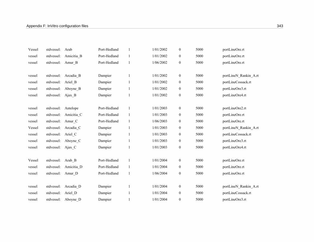
Appendix F: InVitro configuration files 343
Vessel stdvessel: Arab Port-Hedland 1 1/01/2002 0 5000 portLineOre.rt
vessel stdvessel: Amicitia_B Port-Hedland 1 1/01/2002 0 5000 portLineOre.rt
vessel stdvessel: Amur_B Port-Hedland 1 1/06/2002 0 5000 portLineOre.rt
vessel stdvessel: Arcadia_B Dampier 1 1/01/2002 0 5000 portLineN_Rankin_A.rt
vessel stdvessel: Ariel_B Dampier 1 1/01/2002 0 5000 portLineCossack.rt
vessel stdvessel: Aboyne_B Dampier 1 1/01/2002 0 5000 portLineOre3.rt
vessel stdvessel: Ajax_B Dampier 1 1/01/2002 0 5000 portLineOre4.rt
vessel stdvessel: Antelope Port-Hedland 1 1/01/2003 0 5000 portLineOre2.rt
vessel stdvessel: Amicitia_C Port-Hedland 1 1/01/2003 0 5000 portLineOre.rt
vessel stdvessel: Amur_C Port-Hedland 1 1/06/2003 0 5000 portLineOre.rt
Vessel stdvessel: Arcadia_C Dampier 1 1/01/2003 0 5000 portLineN_Rankin_A.rt
vessel stdvessel: Ariel_C Dampier 1 1/01/2003 0 5000 portLineCossack.rt
vessel stdvessel: Aboyne_C Dampier 1 1/01/2003 0 5000 portLineOre3.rt
vessel stdvessel: Ajax_C Dampier 1 1/01/2003 0 5000 portLineOre4.rt
Vessel stdvessel: Arab_B Port-Hedland 1 1/01/2004 0 5000 portLineOre.rt
vessel stdvessel: Amicitia_D Port-Hedland 1 1/01/2004 0 5000 portLineOre.rt
vessel stdvessel: Amur_D Port-Hedland 1 1/06/2004 0 5000 portLineOre.rt
vessel stdvessel: Arcadia_D Dampier 1 1/01/2004 0 5000 portLineN_Rankin_A.rt
vessel stdvessel: Ariel_D Dampier 1 1/01/2004 0 5000 portLineCossack.rt
vessel stdvessel: Aboyne_D Dampier 1 1/01/2004 0 5000 portLineOre3.rt
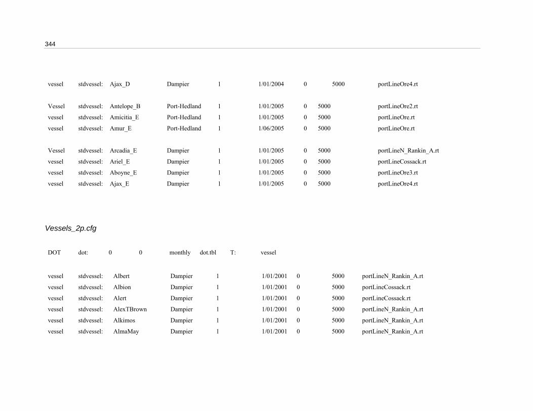
344
vessel stdvessel: Ajax_D Dampier 1 1/01/2004 0 5000 portLineOre4.rt
Vessel stdvessel: Antelope_B Port-Hedland 1 1/01/2005 0 5000 portLineOre2.rt
vessel stdvessel: Amicitia_E Port-Hedland 1 1/01/2005 0 5000 portLineOre.rt
vessel stdvessel: Amur_E Port-Hedland 1 1/06/2005 0 5000 portLineOre.rt
Vessel stdvessel: Arcadia_E Dampier 1 1/01/2005 0 5000 portLineN_Rankin_A.rt
vessel stdvessel: Ariel_E Dampier 1 1/01/2005 0 5000 portLineCossack.rt
vessel stdvessel: Aboyne_E Dampier 1 1/01/2005 0 5000 portLineOre3.rt
vessel stdvessel: Ajax_E Dampier 1 1/01/2005 0 5000 portLineOre4.rt
Vessels_2p.cfg DOT dot: 0 0 monthly dot.tbl T: vessel
vessel stdvessel: Albert Dampier 1 1/01/2001 0 5000 portLineN_Rankin_A.rt
vessel stdvessel: Albion Dampier 1 1/01/2001 0 5000 portLineCossack.rt
vessel stdvessel: Alert Dampier 1 1/01/2001 0 5000 portLineCossack.rt
vessel stdvessel: AlexTBrown Dampier 1 1/01/2001 0 5000 portLineN_Rankin_A.rt
vessel stdvessel: Alkimos Dampier 1 1/01/2001 0 5000 portLineN_Rankin_A.rt
vessel stdvessel: AlmaMay Dampier 1 1/01/2001 0 5000 portLineN_Rankin_A.rt
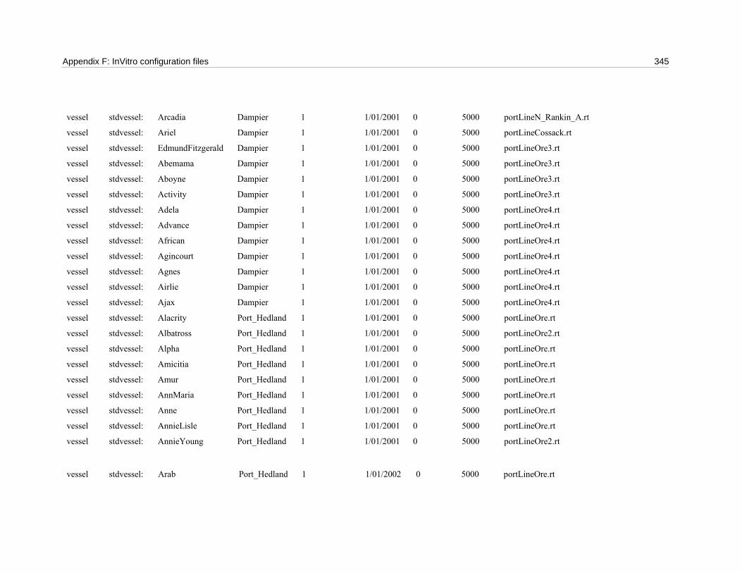
Appendix F: InVitro configuration files 345
vessel stdvessel: Arcadia Dampier 1 1/01/2001 0 5000 portLineN_Rankin_A.rt
vessel stdvessel: Ariel Dampier 1 1/01/2001 0 5000 portLineCossack.rt
vessel stdvessel: EdmundFitzgerald Dampier 1 1/01/2001 0 5000 portLineOre3.rt
vessel stdvessel: Abemama Dampier 1 1/01/2001 0 5000 portLineOre3.rt
vessel stdvessel: Aboyne Dampier 1 1/01/2001 0 5000 portLineOre3.rt
vessel stdvessel: Activity Dampier 1 1/01/2001 0 5000 portLineOre3.rt
vessel stdvessel: Adela Dampier 1 1/01/2001 0 5000 portLineOre4.rt
vessel stdvessel: Advance Dampier 1 1/01/2001 0 5000 portLineOre4.rt
vessel stdvessel: African Dampier 1 1/01/2001 0 5000 portLineOre4.rt
vessel stdvessel: Agincourt Dampier 1 1/01/2001 0 5000 portLineOre4.rt
vessel stdvessel: Agnes Dampier 1 1/01/2001 0 5000 portLineOre4.rt
vessel stdvessel: Airlie Dampier 1 1/01/2001 0 5000 portLineOre4.rt
vessel stdvessel: Ajax Dampier 1 1/01/2001 0 5000 portLineOre4.rt
vessel stdvessel: Alacrity Port_Hedland 1 1/01/2001 0 5000 portLineOre.rt
vessel stdvessel: Albatross Port_Hedland 1 1/01/2001 0 5000 portLineOre2.rt
vessel stdvessel: Alpha Port_Hedland 1 1/01/2001 0 5000 portLineOre.rt
vessel stdvessel: Amicitia Port_Hedland 1 1/01/2001 0 5000 portLineOre.rt
vessel stdvessel: Amur Port_Hedland 1 1/01/2001 0 5000 portLineOre.rt
vessel stdvessel: AnnMaria Port_Hedland 1 1/01/2001 0 5000 portLineOre.rt
vessel stdvessel: Anne Port_Hedland 1 1/01/2001 0 5000 portLineOre.rt
vessel stdvessel: AnnieLisle Port_Hedland 1 1/01/2001 0 5000 portLineOre.rt
vessel stdvessel: AnnieYoung Port_Hedland 1 1/01/2001 0 5000 portLineOre2.rt
vessel stdvessel: Arab Port_Hedland 1 1/01/2002 0 5000 portLineOre.rt
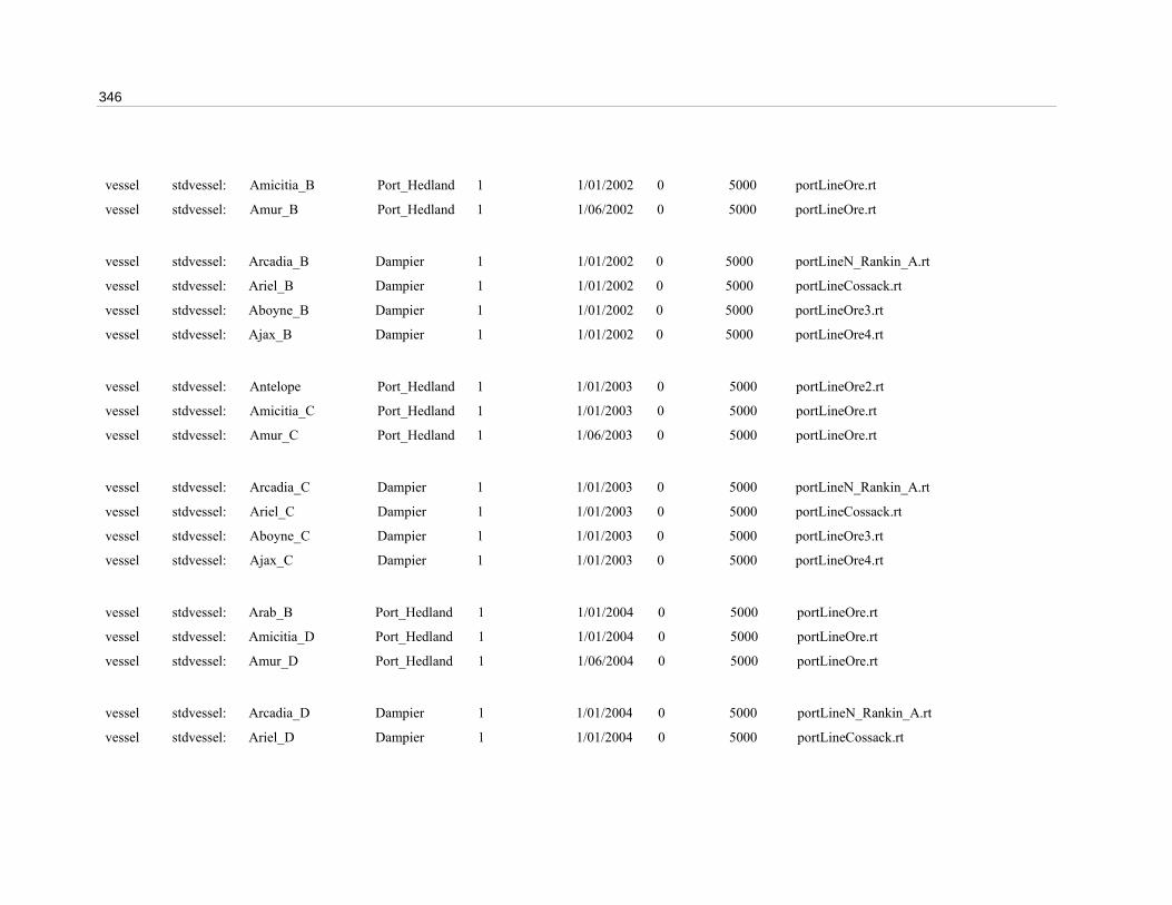
346
vessel stdvessel: Amicitia_B Port_Hedland 1 1/01/2002 0 5000 portLineOre.rt
vessel stdvessel: Amur_B Port_Hedland 1 1/06/2002 0 5000 portLineOre.rt
vessel stdvessel: Arcadia_B Dampier 1 1/01/2002 0 5000 portLineN_Rankin_A.rt
vessel stdvessel: Ariel_B Dampier 1 1/01/2002 0 5000 portLineCossack.rt
vessel stdvessel: Aboyne_B Dampier 1 1/01/2002 0 5000 portLineOre3.rt
vessel stdvessel: Ajax_B Dampier 1 1/01/2002 0 5000 portLineOre4.rt
vessel stdvessel: Antelope Port_Hedland 1 1/01/2003 0 5000 portLineOre2.rt
vessel stdvessel: Amicitia_C Port_Hedland 1 1/01/2003 0 5000 portLineOre.rt
vessel stdvessel: Amur_C Port_Hedland 1 1/06/2003 0 5000 portLineOre.rt
vessel stdvessel: Arcadia_C Dampier 1 1/01/2003 0 5000 portLineN_Rankin_A.rt
vessel stdvessel: Ariel_C Dampier 1 1/01/2003 0 5000 portLineCossack.rt
vessel stdvessel: Aboyne_C Dampier 1 1/01/2003 0 5000 portLineOre3.rt
vessel stdvessel: Ajax_C Dampier 1 1/01/2003 0 5000 portLineOre4.rt
vessel stdvessel: Arab_B Port_Hedland 1 1/01/2004 0 5000 portLineOre.rt
vessel stdvessel: Amicitia_D Port_Hedland 1 1/01/2004 0 5000 portLineOre.rt
vessel stdvessel: Amur_D Port_Hedland 1 1/06/2004 0 5000 portLineOre.rt
vessel stdvessel: Arcadia_D Dampier 1 1/01/2004 0 5000 portLineN_Rankin_A.rt
vessel stdvessel: Ariel_D Dampier 1 1/01/2004 0 5000 portLineCossack.rt
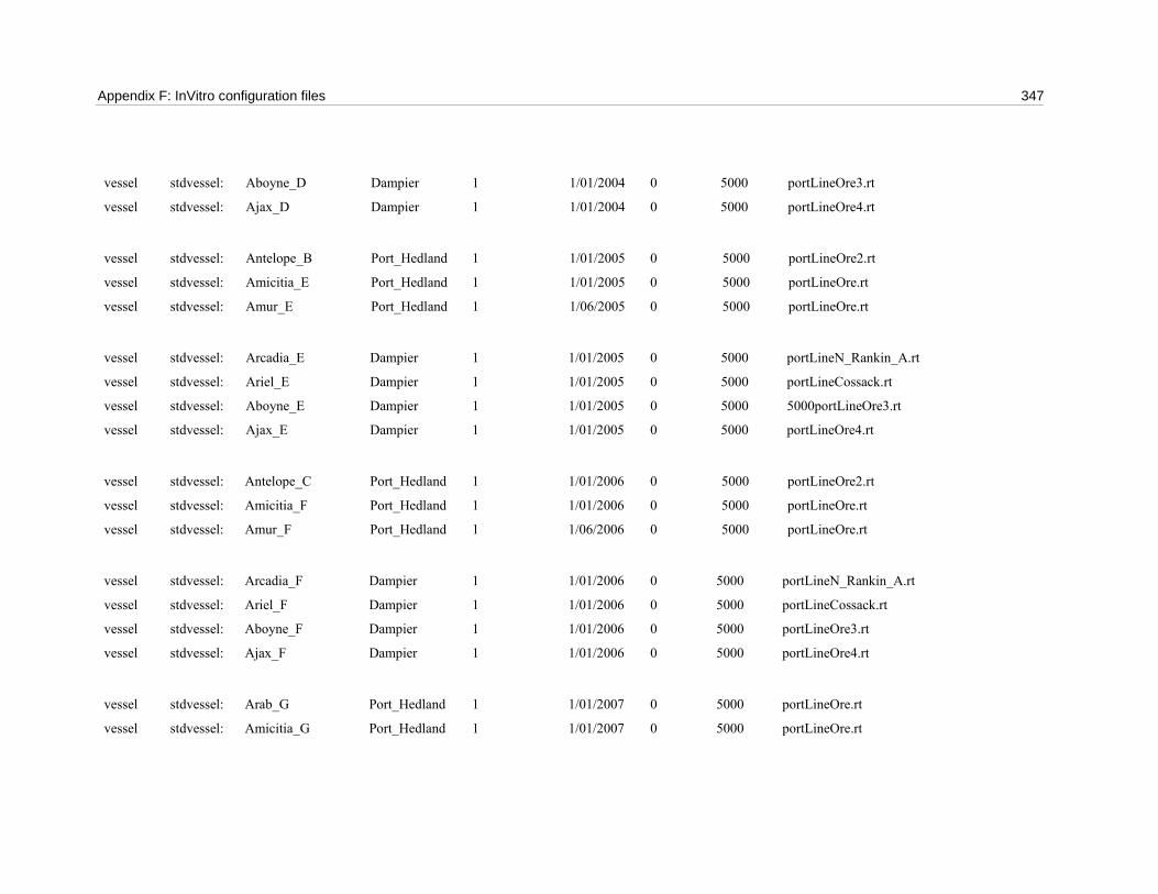
Appendix F: InVitro configuration files 347
vessel stdvessel: Aboyne_D Dampier 1 1/01/2004 0 5000 portLineOre3.rt
vessel stdvessel: Ajax_D Dampier 1 1/01/2004 0 5000 portLineOre4.rt
vessel stdvessel: Antelope_B Port_Hedland 1 1/01/2005 0 5000 portLineOre2.rt
vessel stdvessel: Amicitia_E Port_Hedland 1 1/01/2005 0 5000 portLineOre.rt
vessel stdvessel: Amur_E Port_Hedland 1 1/06/2005 0 5000 portLineOre.rt
vessel stdvessel: Arcadia_E Dampier 1 1/01/2005 0 5000 portLineN_Rankin_A.rt
vessel stdvessel: Ariel_E Dampier 1 1/01/2005 0 5000 portLineCossack.rt
vessel stdvessel: Aboyne_E Dampier 1 1/01/2005 0 5000 5000portLineOre3.rt
vessel stdvessel: Ajax_E Dampier 1 1/01/2005 0 5000 portLineOre4.rt
vessel stdvessel: Antelope_C Port_Hedland 1 1/01/2006 0 5000 portLineOre2.rt
vessel stdvessel: Amicitia_F Port_Hedland 1 1/01/2006 0 5000 portLineOre.rt
vessel stdvessel: Amur_F Port_Hedland 1 1/06/2006 0 5000 portLineOre.rt
vessel stdvessel: Arcadia_F Dampier 1 1/01/2006 0 5000 portLineN_Rankin_A.rt
vessel stdvessel: Ariel_F Dampier 1 1/01/2006 0 5000 portLineCossack.rt
vessel stdvessel: Aboyne_F Dampier 1 1/01/2006 0 5000 portLineOre3.rt
vessel stdvessel: Ajax_F Dampier 1 1/01/2006 0 5000 portLineOre4.rt
vessel stdvessel: Arab_G Port_Hedland 1 1/01/2007 0 5000 portLineOre.rt
vessel stdvessel: Amicitia_G Port_Hedland 1 1/01/2007 0 5000 portLineOre.rt

348
vessel stdvessel: Amur_G Port_Hedland 1 1/06/2007 0 5000 portLineOre.rt
vessel stdvessel: Arcadia_G Dampier 1 1/01/2007 0 5000 portLineN_Rankin_A.rt
vessel stdvessel: Ariel_G Dampier 1 1/01/2007 0 5000 portLineCossack.rt
vessel stdvessel: Aboyne_G Dampier 1 1/01/2007 0 500 5000portLineOre3.rt
vessel stdvessel: Ajax_G Dampier 1 1/01/2007 0 5000 portLineOre4.rt
vessel stdvessel: Antelope_H Port_Hedland 1 1/01/2008 0 5000 portLineOre2.rt
vessel stdvessel: Amicitia_H Port_Hedland 1 1/01/2008 0 5000 portLineOre.rt
vessel stdvessel: Amur_H Port_Hedland 1 1/01/2008 0 5000 portLineOre.rt
vessel stdvessel: Arcadia_H Dampier 1 1/01/2008 0 5000 portLineN_Rankin_A.rt
vessel stdvessel: Ariel_H Dampier 1 1/01/2008 0 5000 portLineCossack.rt
vessel stdvessel: Aboyne_H Dampier 1 1/01/2008 0 5000 portLineOre3.rt
vessel stdvessel: Ajax_H Dampier 1 1/01/2008 0 5000 portLineOre4.rt
vessel stdvessel: Anne_I Port_Hedland 1 1/01/2009 0 5000 portLineOre.rt
vessel stdvessel: AnnieLisle_I Port_Hedland 1 1/01/2009 0 5000 portLineOre.rt
vessel stdvessel: AnnieYoung_I Port_Hedland 1 1/01/2009 0 5000 portLineOre2.rt
vessel stdvessel: Arcadia_I Dampier 1 1/01/2009 0 5000 portLineN_Rankin_A.rt
vessel stdvessel: Ariel_I Dampier 1 1/01/2009 0 5000 portLineCossack.rt
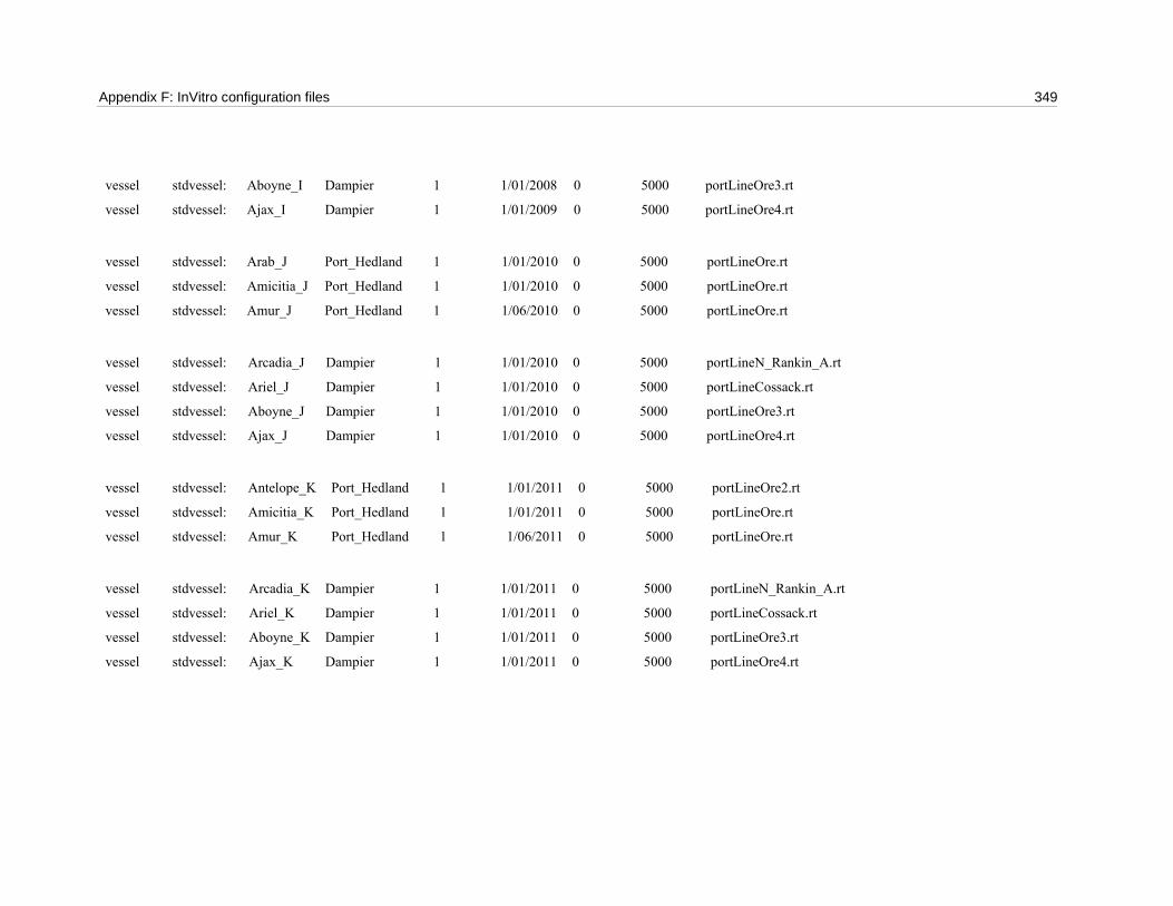
Appendix F: InVitro configuration files 349
vessel stdvessel: Aboyne_I Dampier 1 1/01/2008 0 5000 portLineOre3.rt
vessel stdvessel: Ajax_I Dampier 1 1/01/2009 0 5000 portLineOre4.rt
vessel stdvessel: Arab_J Port_Hedland 1 1/01/2010 0 5000 portLineOre.rt
vessel stdvessel: Amicitia_J Port_Hedland 1 1/01/2010 0 5000 portLineOre.rt
vessel stdvessel: Amur_J Port_Hedland 1 1/06/2010 0 5000 portLineOre.rt
vessel stdvessel: Arcadia_J Dampier 1 1/01/2010 0 5000 portLineN_Rankin_A.rt
vessel stdvessel: Ariel_J Dampier 1 1/01/2010 0 5000 portLineCossack.rt
vessel stdvessel: Aboyne_J Dampier 1 1/01/2010 0 5000 portLineOre3.rt
vessel stdvessel: Ajax_J Dampier 1 1/01/2010 0 5000 portLineOre4.rt
vessel stdvessel: Antelope_K Port_Hedland 1 1/01/2011 0 5000 portLineOre2.rt
vessel stdvessel: Amicitia_K Port_Hedland 1 1/01/2011 0 5000 portLineOre.rt
vessel stdvessel: Amur_K Port_Hedland 1 1/06/2011 0 5000 portLineOre.rt
vessel stdvessel: Arcadia_K Dampier 1 1/01/2011 0 5000 portLineN_Rankin_A.rt
vessel stdvessel: Ariel_K Dampier 1 1/01/2011 0 5000 portLineCossack.rt
vessel stdvessel: Aboyne_K Dampier 1 1/01/2011 0 5000 portLineOre3.rt
vessel stdvessel: Ajax_K Dampier 1 1/01/2011 0 5000 portLineOre4.rt
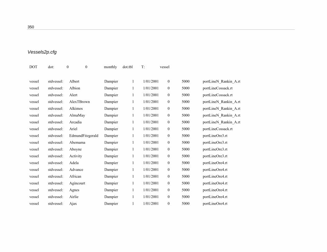
350
Vessels2p.cfg DOT dot: 0 0 monthly dot.tbl T: vessel
vessel stdvessel: Albert Dampier 1 1/01/2001 0 5000 portLineN_Rankin_A.rt
vessel stdvessel: Albion Dampier 1 1/01/2001 0 5000 portLineCossack.rt
vessel stdvessel: Alert Dampier 1 1/01/2001 0 5000 portLineCossack.rt
vessel stdvessel: AlexTBrown Dampier 1 1/01/2001 0 5000 portLineN_Rankin_A.rt
vessel stdvessel: Alkimos Dampier 1 1/01/2001 0 5000 portLineN_Rankin_A.rt
vessel stdvessel: AlmaMay Dampier 1 1/01/2001 0 5000 portLineN_Rankin_A.rt
vessel stdvessel: Arcadia Dampier 1 1/01/2001 0 5000 portLineN_Rankin_A.rt
vessel stdvessel: Ariel Dampier 1 1/01/2001 0 5000 portLineCossack.rt
vessel stdvessel: EdmundFitzgerald Dampier 1 1/01/2001 0 5000 portLineOre3.rt
vessel stdvessel: Abemama Dampier 1 1/01/2001 0 5000 portLineOre3.rt
vessel stdvessel: Aboyne Dampier 1 1/01/2001 0 5000 portLineOre3.rt
vessel stdvessel: Activity Dampier 1 1/01/2001 0 5000 portLineOre3.rt
vessel stdvessel: Adela Dampier 1 1/01/2001 0 5000 portLineOre4.rt
vessel stdvessel: Advance Dampier 1 1/01/2001 0 5000 portLineOre4.rt
vessel stdvessel: African Dampier 1 1/01/2001 0 5000 portLineOre4.rt
vessel stdvessel: Agincourt Dampier 1 1/01/2001 0 5000 portLineOre4.rt
vessel stdvessel: Agnes Dampier 1 1/01/2001 0 5000 portLineOre4.rt
vessel stdvessel: Airlie Dampier 1 1/01/2001 0 5000 portLineOre4.rt
vessel stdvessel: Ajax Dampier 1 1/01/2001 0 5000 portLineOre4.rt
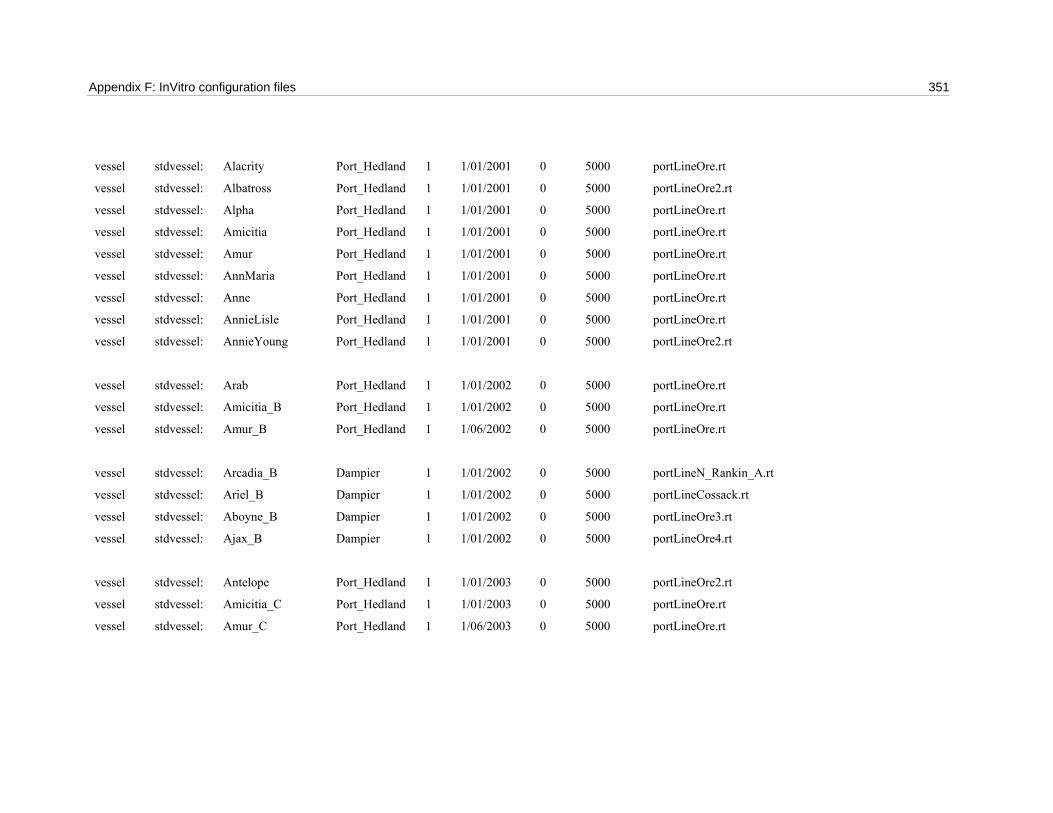
Appendix F: InVitro configuration files 351
vessel stdvessel: Alacrity Port_Hedland 1 1/01/2001 0 5000 portLineOre.rt
vessel stdvessel: Albatross Port_Hedland 1 1/01/2001 0 5000 portLineOre2.rt
vessel stdvessel: Alpha Port_Hedland 1 1/01/2001 0 5000 portLineOre.rt
vessel stdvessel: Amicitia Port_Hedland 1 1/01/2001 0 5000 portLineOre.rt
vessel stdvessel: Amur Port_Hedland 1 1/01/2001 0 5000 portLineOre.rt
vessel stdvessel: AnnMaria Port_Hedland 1 1/01/2001 0 5000 portLineOre.rt
vessel stdvessel: Anne Port_Hedland 1 1/01/2001 0 5000 portLineOre.rt
vessel stdvessel: AnnieLisle Port_Hedland 1 1/01/2001 0 5000 portLineOre.rt
vessel stdvessel: AnnieYoung Port_Hedland 1 1/01/2001 0 5000 portLineOre2.rt
vessel stdvessel: Arab Port_Hedland 1 1/01/2002 0 5000 portLineOre.rt
vessel stdvessel: Amicitia_B Port_Hedland 1 1/01/2002 0 5000 portLineOre.rt
vessel stdvessel: Amur_B Port_Hedland 1 1/06/2002 0 5000 portLineOre.rt
vessel stdvessel: Arcadia_B Dampier 1 1/01/2002 0 5000 portLineN_Rankin_A.rt
vessel stdvessel: Ariel_B Dampier 1 1/01/2002 0 5000 portLineCossack.rt
vessel stdvessel: Aboyne_B Dampier 1 1/01/2002 0 5000 portLineOre3.rt
vessel stdvessel: Ajax_B Dampier 1 1/01/2002 0 5000 portLineOre4.rt
vessel stdvessel: Antelope Port_Hedland 1 1/01/2003 0 5000 portLineOre2.rt
vessel stdvessel: Amicitia_C Port_Hedland 1 1/01/2003 0 5000 portLineOre.rt
vessel stdvessel: Amur_C Port_Hedland 1 1/06/2003 0 5000 portLineOre.rt
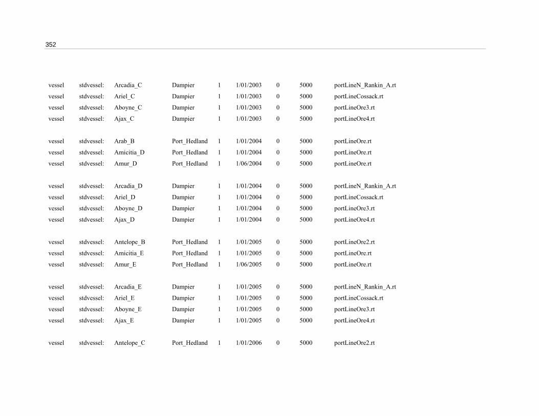
352
vessel stdvessel: Arcadia_C Dampier 1 1/01/2003 0 5000 portLineN_Rankin_A.rt
vessel stdvessel: Ariel_C Dampier 1 1/01/2003 0 5000 portLineCossack.rt
vessel stdvessel: Aboyne_C Dampier 1 1/01/2003 0 5000 portLineOre3.rt
vessel stdvessel: Ajax_C Dampier 1 1/01/2003 0 5000 portLineOre4.rt
vessel stdvessel: Arab_B Port_Hedland 1 1/01/2004 0 5000 portLineOre.rt
vessel stdvessel: Amicitia_D Port_Hedland 1 1/01/2004 0 5000 portLineOre.rt
vessel stdvessel: Amur_D Port_Hedland 1 1/06/2004 0 5000 portLineOre.rt
vessel stdvessel: Arcadia_D Dampier 1 1/01/2004 0 5000 portLineN_Rankin_A.rt
vessel stdvessel: Ariel_D Dampier 1 1/01/2004 0 5000 portLineCossack.rt
vessel stdvessel: Aboyne_D Dampier 1 1/01/2004 0 5000 portLineOre3.rt
vessel stdvessel: Ajax_D Dampier 1 1/01/2004 0 5000 portLineOre4.rt
vessel stdvessel: Antelope_B Port_Hedland 1 1/01/2005 0 5000 portLineOre2.rt
vessel stdvessel: Amicitia_E Port_Hedland 1 1/01/2005 0 5000 portLineOre.rt
vessel stdvessel: Amur_E Port_Hedland 1 1/06/2005 0 5000 portLineOre.rt
vessel stdvessel: Arcadia_E Dampier 1 1/01/2005 0 5000 portLineN_Rankin_A.rt
vessel stdvessel: Ariel_E Dampier 1 1/01/2005 0 5000 portLineCossack.rt
vessel stdvessel: Aboyne_E Dampier 1 1/01/2005 0 5000 portLineOre3.rt
vessel stdvessel: Ajax_E Dampier 1 1/01/2005 0 5000 portLineOre4.rt
vessel stdvessel: Antelope_C Port_Hedland 1 1/01/2006 0 5000 portLineOre2.rt
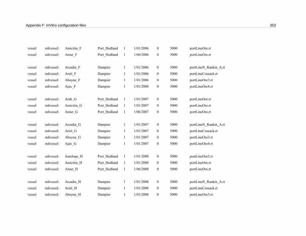
Appendix F: InVitro configuration files 353
vessel stdvessel: Amicitia_F Port_Hedland 1 1/01/2006 0 5000 portLineOre.rt
vessel stdvessel: Amur_F Port_Hedland 1 1/06/2006 0 5000 portLineOre.rt
vessel stdvessel: Arcadia_F Dampier 1 1/01/2006 0 5000 portLineN_Rankin_A.rt
vessel stdvessel: Ariel_F Dampier 1 1/01/2006 0 5000 portLineCossack.rt
vessel stdvessel: Aboyne_F Dampier 1 1/01/2006 0 5000 portLineOre3.rt
vessel stdvessel: Ajax_F Dampier 1 1/01/2006 0 5000 portLineOre4.rt
vessel stdvessel: Arab_G Port_Hedland 1 1/01/2007 0 5000 portLineOre.rt
vessel stdvessel: Amicitia_G Port_Hedland 1 1/01/2007 0 5000 portLineOre.rt
vessel stdvessel: Amur_G Port_Hedland 1 1/06/2007 0 5000 portLineOre.rt
vessel stdvessel: Arcadia_G Dampier 1 1/01/2007 0 5000 portLineN_Rankin_A.rt
vessel stdvessel: Ariel_G Dampier 1 1/01/2007 0 5000 portLineCossack.rt
vessel stdvessel: Aboyne_G Dampier 1 1/01/2007 0 5000 portLineOre3.rt
vessel stdvessel: Ajax_G Dampier 1 1/01/2007 0 5000 portLineOre4.rt
vessel stdvessel: Antelope_H Port_Hedland 1 1/01/2008 0 5000 portLineOre2.rt
vessel stdvessel: Amicitia_H Port_Hedland 1 1/01/2008 0 5000 portLineOre.rt
vessel stdvessel: Amur_H Port_Hedland 1 1/06/2008 0 5000 portLineOre.rt
vessel stdvessel: Arcadia_H Dampier 1 1/01/2008 0 5000 portLineN_Rankin_A.rt
vessel stdvessel: Ariel_H Dampier 1 1/01/2008 0 5000 portLineCossack.rt
vessel stdvessel: Aboyne_H Dampier 1 1/01/2008 0 5000 portLineOre3.rt

354
vessel stdvessel: Ajax_H Dampier 1 1/01/2008 0 5000 portLineOre4.rt
vessel stdvessel: Anne_I Port_Hedland 1 1/01/2009 0 5000 portLineOre.rt
vessel stdvessel: AnnieLisle_I Port_Hedland 1 1/01/2009 0 5000 portLineOre.rt
vessel stdvessel: AnnieYoung_I Port_Hedland 1 1/01/2009 0 5000 portLineOre2.rt
vessel stdvessel: Arcadia_I Dampier 1 1/01/2009 0 5000 portLineN_Rankin_A.rt
vessel stdvessel: Ariel_I Dampier 1 1/01/2009 0 5000 portLineCossack.rt
vessel stdvessel: Aboyne_I Dampier 1 1/01/2009 0 5000 portLineOre3.rt
vessel stdvessel: Ajax_I Dampier 1 1/01/2009 0 5000 portLineOre4.rt
vessel stdvessel: Arab_J Port_Hedland 1 1/01/2010 0 5000 portLineOre.rt
vessel stdvessel: Amicitia_J Port_Hedland 1 1/01/2010 0 5000 portLineOre.rt
vessel stdvessel: Amur_J Port_Hedland 1 1/06/2010 0 5000 portLineOre.rt
vessel stdvessel: Arcadia_J Dampier 1 1/01/2010 0 5000 portLineN_Rankin_A.rt
vessel stdvessel: Ariel_J Dampier 1 1/01/2010 0 5000 portLineCossack.rt
vessel stdvessel: Aboyne_J Dampier 1 1/01/2010 0 5000 portLineOre3.rt
vessel stdvessel: Ajax_J Dampier 1 1/01/2010 0 5000 portLineOre4.rt
vessel stdvessel: Antelope_K Port_Hedland 1 1/01/2011 0 5000 portLineOre2.rt
vessel stdvessel: Amicitia_K Port_Hedland 1 1/01/2011 0 5000 portLineOre.rt
vessel stdvessel: Amur_K Port_Hedland 1 1/06/2011 0 5000 portLineOre.rt
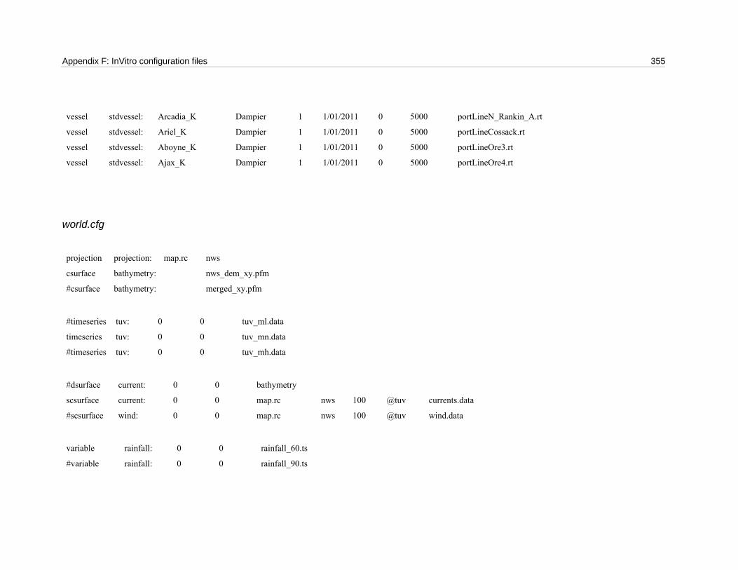
Appendix F: InVitro configuration files 355
vessel stdvessel: Arcadia_K Dampier 1 1/01/2011 0 5000 portLineN_Rankin_A.rt
vessel stdvessel: Ariel_K Dampier 1 1/01/2011 0 5000 portLineCossack.rt
vessel stdvessel: Aboyne_K Dampier 1 1/01/2011 0 5000 portLineOre3.rt
vessel stdvessel: Ajax_K Dampier 1 1/01/2011 0 5000 portLineOre4.rt
world.cfg projection projection: map.rc nws
csurface bathymetry: nws_dem_xy.pfm
#csurface bathymetry: merged_xy.pfm
#timeseries tuv: 0 0 tuv_ml.data
timeseries tuv: 0 0 tuv_mn.data
#timeseries tuv: 0 0 tuv_mh.data
#dsurface current: 0 0 bathymetry
scsurface current: 0 0 map.rc nws 100 @tuv currents.data
#scsurface wind: 0 0 map.rc nws 100 @tuv wind.data
variable rainfall: 0 0 rainfall_60.ts
#variable rainfall: 0 0 rainfall_90.ts
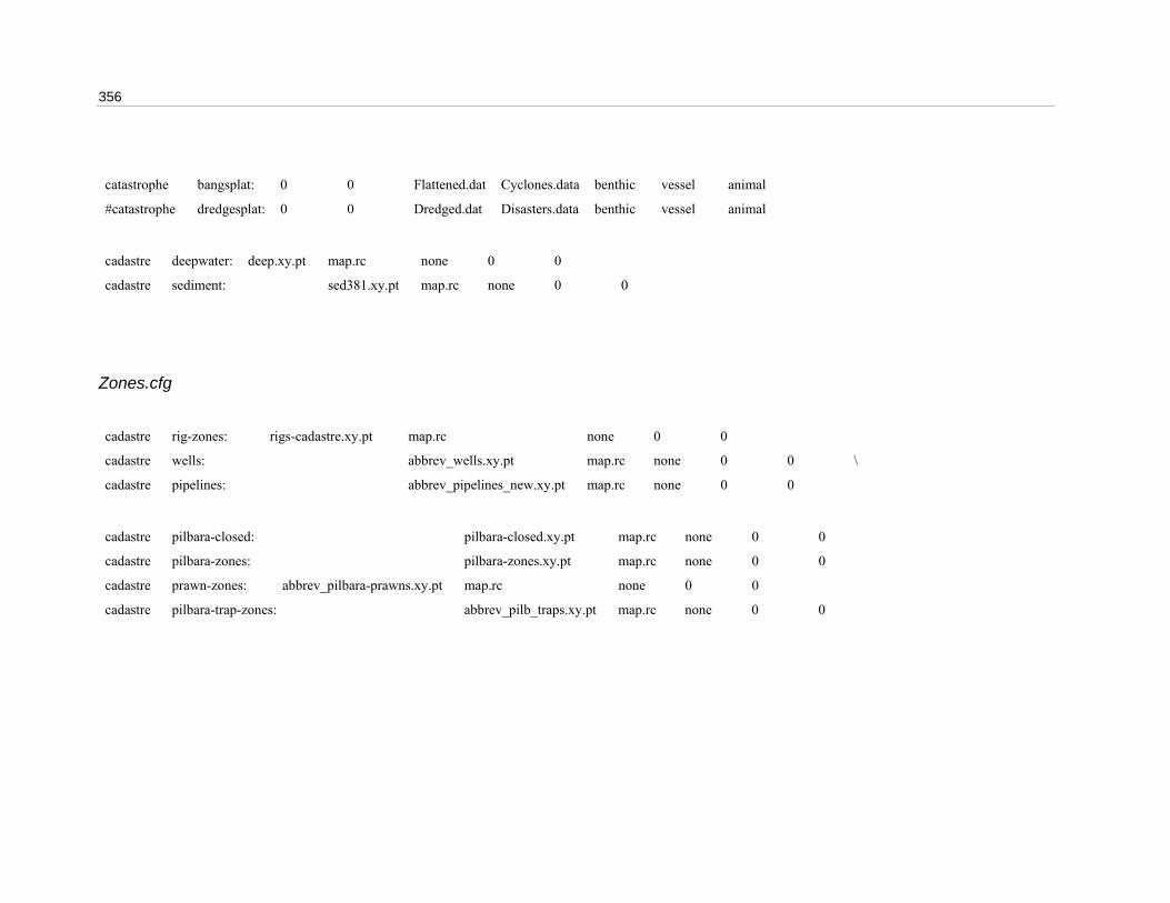
356
catastrophe bangsplat: 0 0 Flattened.dat Cyclones.data benthic vessel animal
#catastrophe dredgesplat: 0 0 Dredged.dat Disasters.data benthic vessel animal
cadastre deepwater: deep.xy.pt map.rc none 0 0
cadastre sediment: sed381.xy.pt map.rc none 0 0
Zones.cfg cadastre rig-zones: rigs-cadastre.xy.pt map.rc none 0 0
cadastre wells: abbrev_wells.xy.pt map.rc none 0 0 \
cadastre pipelines: abbrev_pipelines_new.xy.pt map.rc none 0 0
cadastre pilbara-closed: pilbara-closed.xy.pt map.rc none 0 0
cadastre pilbara-zones: pilbara-zones.xy.pt map.rc none 0 0
cadastre prawn-zones: abbrev_pilbara-prawns.xy.pt map.rc none 0 0
cadastre pilbara-trap-zones: abbrev_pilb_traps.xy.pt map.rc none 0 0
Acknowledgments 357
ACKNOWLEDGMENTS
The authors would like to thank Linda Thomas, William Upcher and Brendon Ward for their assistance in compiling this report.
This study was funded by the Western Australia Department of Environmental Protection as part of the North West Shelf Marine Environmental Management Study. AIMS and CSIRO Marine Research provided in-kind support.
Clodagh Jones worked to improve the accuracy, consistency, and editorial style of the bibliography. We are grateful to all of those who supplied us with references, publications and suggestions for research needs.
The following people and agencies have contributed significantly to the Study through the provision of technical expertise and advice, and historical data and information. The Study partners gratefully acknowledge their contribution.
Western Australian State agencies Department of Environment and Conservation (Department of Conservation and Land Management and Department of Environment) Department of Fisheries Department of Industry and Resources (Department of Mineral and Petroleum Resources) Department of Land Information Department for Planning and Infrastructure (Department of Transport) Pilbara Tourism Association Shire of Roebourne Town of Port Hedland Tourism Western Australia Western Australian Land Information System Western Australian Museum
Commonwealth agencies Australian Institute of Marine Science Geoscience Australia (formerly Australian Geological Survey Organisation)
Consultants Cognito Consulting David Gordon International Risk Consultants METOCEAN Engineers (formerly Weather News International, Perth) Oceanica (formerly DA Lord and Associates)
Industries Australian Petroleum Production Exploration Association (APPEA) Apache Energy BHP Petroleum Chevron Australia Dampier Salt Hamersley Iron Mermaid Marine Woodside Energy

358
Individuals Clay Bryce Graham Cobby Nick D’Adamo Mike Forde David Gordon Andrew Heyward Barry Hutchins Bryan Jenkins Di Jones Ian LeProvost Ray Masini Mike Moran Steve Newman Eric Paling Kelly Pendoley Bob Prinz Chris Simpson Shirley Slack-Smith Di Walker
Editorial and publishing Louise Bell – Graphics/cover design Lea Crosswell – Webpage design Rob McKenzie – Editor Diana Reale – Webpage design Linda Thomas – Editorial consultant/layout and design Helen Webb – Editorial consultant/Project Manager
Front cover photos courtesy of: Centre – Coral reef ecosystem, WA Museum, Clay Bryce Aquaculture pearls, Department of Fisheries WA Recreational fishing, Department of Fisheries WA, Jirri Lockman Offshore petroleum platform, Woodside Energy Ltd Commercial Fishing, Department of Fisheries WA Tourism, CSIRO Coastal development aerial photos, Hamersley Iron Pty Ltd
