Man vs. Machine:

Quantitative and Discretionary Equity Management∗

Simona Abis

Columbia University

May 28, 2018

Abstract

I use a machine learning technique to classify the universe of active US equity mutual

funds as �quantitative�, who mostly rely of computer-driven models and �xed rules, or

�discretionary�, who mostly rely on human judgement. I �rst document several new facts

about quantitative investing. I then propose an equilibrium model in which quantitative

funds have a greater information processing capacity but follow less �exible strategies

than discretionary funds. The model predicts that quantitative funds specialize in stock

picking, hold more stocks, display pro-cyclical performance, and that their trades are

vulnerable to �overcrowding�. In contrast, discretionary funds alternate between stock

picking and market timing, display counter-cyclical performance and focus on stocks

for which less overall information is available. My empirical evidence supports these

predictions.

∗Correspondence: Simona Abis, Columbia University, 3022 Broadway, Uris 420, New York, NY 10027. E-mail:sa3518@columbia.edu. I wish to thank Joël Peress for his support and invaluable advice. I am grateful for thevery helpful comments from Lily Fang, Thierry Foucault, Sergei Glebkin, Jillian Grennan, Denis Gromb, MarcinKacperczyk, John Kuong, Hugues Langlois, Harry Mamaysky, Alberto Rossi, Rafael Zambrana and Qi Zeng. I alsothank Adrian Buss, Theodoros Evgeniou, Federico Gavazzoni, Naveen Ghondi, Massimo Massa, Ioanid Rosu, LucieTepla, Theo Vermaelen, Bart Yueshen, and Hong Zhang as well as seminar participants at INSEAD brownbags, theLabEx PhD consortium, the HEC PhD Workshop, the INSEAD-Wharton Consortium, the AQR Institute AcademicSymposium at LBS, the WAPFIN conference, the Nova-BPI Asset Management Conference and the Maryland JuniorFinance Conference. I am responsible for any errors.

1 Introduction

Advances in computational technology and data analytics are revolutionizing the asset management

industry and give every indication of con- tinuing to do so (World Economic Forum 2015, Chui,

Manyika, and Miremadi 2016). As David Siegel, co-head of Two Sigma, a prominent hedge fund,

puts it: �The challenge facing the investment world is that the human mind has not become any

better than it was 100 years ago, and it's very hard for someone using traditional methods to juggle

all the information of the global economy in their head (. . . ). Eventually the time will come that

no human investment manager will be able to beat the computer�. Yet little is known about the

prevalence of quantitative strategies in the mutual fund industry, their e�ect on fund performance,

and their in�uence, if any, on asset prices. My paper �lls this gap by carrying out a detailed analysis

of quantitative investing in the US equity mutual fund universe.

The �rst step of my analysis is to develop a novel methodology to classify funds as quantitative

or discretionary (i.e., non-quantitative). Here quantitative funds are those basing their investment

processes primarily on quantitative signals generated by computer-driven models using �xed rules

to analyze large datasets. Instead, discretionary funds rely mostly on decisions by asset managers

who use information and their own judgment. I collect mutual fund prospectuses for 2,607 funds

from 1999 to 2015 from the Securities and Exchange Commission (SEC). I manually categorize using

objective criteria a subsample of 200 funds, which then serves as a training sample for a machine

learning algorithm. That procedure results in a dataset of 599 quantitative and 1,851 discretionary

funds.

The classi�cation then allows me to report a number of stylized facts about quantitative funds. I

�nd that they have quintupled in number and more than quadrupled in size over 1999�2015, growing

at double the rate as discretionary funds. Currently their total assets under management (AuM)

amount to $412 bn�or roughly 14% of the AuM of US equity mutual funds. Since 2011, in particular,

capital has been �owing from discretionary to quantitative funds. On average, quantitative funds

are younger (13.0 vs. 14.5 years) and smaller ($552 mm vs. $1.2 bn); they charge 10% lower expense

ratios and 9% lower management fees, exhibit 10% higher turnover, own stocks that load more on

value and momentum factors, and hold less cash than discretionary funds. They also experience

out�ows during recessions that are signi�cantly stronger than those experienced by discretionary

funds.1

I focus next on understanding how quantitative funds di�er from their discretionary peers in terms of

investment style and performance, and on how their growing importance might a�ect stock markets.

One might expect quantitative funds to hold portfolios that are less susceptible to human managers'

limited information processing capacity. On the other hand, these funds might be less �exible in

adapting their strategies to changing market conditions, and their trades might be more correlated

(Khandani and Lo 2011).

1All di�erences are signi�cant at the 1% level.

1

To guide my analysis of investment style and performance, I extend the model by Kacperczyk, Van

Nieuwerburgh, and Veldkamp 2016 (hereafter KVV). Theirs is a static general equilibrium model

with multiple assets subject to a common aggregate shock and individual idiosyncratic shocks. These

assets are traded by two categories of agents: skilled investors, and unskilled investors. Skilled

investors have limited learning capacity, which they allocate to learning about idiosyncratic shocks

(stock picking) or aggregate shocks (market timing). KVV show that skilled investors optimally focus

their learning on the aggregate shock in recessions, modeled as periods of greater risk aversion and

higher volatility of the aggregate shock2, and on idiosyncratic shocks in expansions. The intuition

is that the marginal bene�t of learning about a shock increases with its volatility. So in recessions,

when the aggregate shock volatility rises, the incentive to learn about it increases. This e�ect is

magni�ed by the much larger supply of the aggregate shock (i.e., since it a�ects all stocks).

I interpret KVV's skilled investors as being discretionary investors. I then add to their model a

second group of skilled investors: quantitative investors, whom I assume to have unlimited learning

capacity but to only be able to learn about idiosyncratic shocks. This key assumption is motivated

by survey evidence (Fabozzi, Focardi, and Jonas 2008a) and by my textual analysis of prospectuses.

Both pieces of evidence indicate that quantitative equity funds tend to specialize in stock-speci�c

information and to incorporate marketwide dynamics in their models via price-based signals such

as momentum.3 Given the importance of this assumption for my analysis, I will further test its

plausibility in the data.4 The model yields seven testable predictions.

1. The presence of quantitative investors mitigates the pattern uncovered by KVV, whereby dis-

cretionary investors switch the focus of their learning across the business cycle. If quantitative

investors represent a large enough share of the market, then discretionary investors instead choose

to specialize in learning about the aggregate shock. This pattern re�ects a substitution e�ect: the

more investors learn about a given shock, the lower the value to others of learning about it.

2. Quantitative investors hold a larger number of stocks than discretionary investors. The reason

is that investors optimally hold those assets about which their signals are more precise. Because

of their unlimited capacity to learn about idiosyncratic shocks, quantitative investors have greater

signal precision regarding the payo�s of more assets; hence it is optimal to hold more of them.

3. When learning about idiosyncratic shocks, discretionary investors focus on stocks for which

relatively less information can be learned. That approach allows them to reduce their information

2Various studies have shown that: aggregate stock market volatility is higher in recessions (Hamilton and Lin1996; Campbell et al. 2001; Engle and Rangel 2008); risk premia and Sharpe ratios are counter-cyclical (Fama andFrench 1989; Cochrane 2006; Ludvigson and Ng 2009; Lettau and Ludvigson 2010); and aggregate risk aversion risesin recessions (Dumas 1989; Chan and Kogan 2002; Garleanu and Panageas 2015).

3Although this assumption is plausible for modeling equity mutual funds, it may be questionable in the contextof some hedge funds (e.g. quantitative macro funds specialize in timing the market using trend-following signals andsignals derived from the analysis of macroeconomic information).

4I report below two �ndings supporting this hypothesis. First, I �nd that quantitative funds that display consis-tently high stock-picking ability in expansions do not switch to displaying high market-timing ability in recessions,indicating that these funds indeed are not �exible in changing the focus of their strategies. Second, I �nd that that nofunds consistently display high market-timing ability throughout the business cycle, indicating in turn that no fundis endowed with the ability to learn only about aggregate shocks.

2

disadvantage, or information gap, relative to quantitative investors.

4. Dispersion of opinion, and hence of holdings, is greater among discretionary investors than

among quantitative investors. This follows from discretionary investors' limited learning capacity

which they need to allocate optimally across shocks. They might choose to learn about di�erent

shocks, as the marginal bene�t of learning about shocks is decreasing in the average precision of

private signals about those shocks in the market � substitution e�ect. This leads to more disperse

portfolio allocations.

5. Quantitative investors display pro-cyclical performance. In expansions, though, two counteracting

e�ects are at play: higher signal precision about idiosyncratic shocks (which, in expansions, matter

more than the aggregate shock) helps quantitative investors outperform the market; but if the

fraction and signal precision of quantitative investors are too high, their advantage is eroded and

they tend to underperform.

6. Performance is counter-cyclical for discretionary investors (as in KVV) thanks to their superior

information about the aggregate shock, which is more relevant in recessions. As the share of quan-

titative investors rises, their performance is worsened in expansions and improved in recessions, due

to a substitution e�ect.

7. As the share of quantitative investors increases, so does the price informativeness of idiosyn-

cratic shocks. However, the e�ect on the aggregate shock's price informativeness varies over the

business cycle. In expansions, aggregate price informativeness is enhanced but only when the share

of quantitative investors is high enough that discretionary investors are induced to specialize in

learning about the aggregate shock (Prediction 2). In recessions, aggregate price informativeness

always decreases with the share of quantitative investors; this is because an increase in the share

of quantitative investors reduces that of discretionary investors, who are the only investors able to

learn about the aggregate shock.

To test these predictions, I merge my sample with the CRSP mutual fund and stock databases, the

Thompson Financial Spectrum dataset, the CRSP Mutual Fund Holdings dataset, IBES analysts

forecasts, and Dow Jones news.

First, I study the extent to which funds engage in stock picking and market timing measured, as in

KVV, by the covariance of fund holdings with future earnings surprises and with future growth in

industrial production respectively.

To begin with, I �nd that KVV's prediction applies only to funds I classify as discretionary: such

funds that display consistently high stock-picking ability in expansions also show high market-timing

ability in recessions (68% higher than the average fund).

Next I test the plausibility of my new key assumption�that is, quantitative funds only learn about

idiosyncratic shocks. Quantitative funds that display consistently high stock-picking ability in ex-

pansions do not display high market timing ability in recessions, and no funds consistently display

high market-timing ability throughout the business cycle. These �ndings lend support to the model's

3

assumption about funds' learning technologies by suggesting, respectively, that quantitative funds

do not �exibly adapt the focus of their learning throughout the business cycle, and that no fund is

endowed with the ability to learn only about aggregate shocks.

Finally, in accordance with Prediction 1, I �nd that, with increases in the share of quantitative

funds (measured as the relative TNA that quantitative funds manage or as the fraction of the US

stock market capitalization held by quantitative funds in my sample), the stock-picking ability of

discretionary funds in expansions decreases signi�cantly (by one standard deviation for every 17%

increase in the share of quantitative funds) and their market-timing ability in recessions increases

signi�cantly (by one standard deviation for every 6.8% increase in the share of quantitative funds).

Second, I �nd that quantitative funds on average hold considerably more stocks than do discretionary

funds (225 vs. 117). Additionally, the distribution of quantitative funds' number of holdings is more

skewed, with a signi�cant portion of funds holding up to 1000 stocks. This translates into greater

portfolio diversi�cation, and hence lower idiosyncratic volatility (up to 15% less). This result is in

line with Prediction 2.

Third, I proxy for the average information gap in the stocks held by quantitative and discretionary

funds with their average size, age, media mentions and analysts coverage. The idea is that more

information is available about stocks for which there exists a longer history and that enjoy greater me-

dia and analyst coverage, making such stocks more easily processable with quantitative approaches;

hence the information gap should be greater. I �nd that the information gap is smaller for the stocks

held by discretionary funds; they hold stocks that are younger (44 months younger than the 351

months average) and have fewer monthly mentions in the media (31 fewer than the 275 average).5

Although there is no signi�cant di�erence in analyst coverage, I �nd that all funds holding stocks

less mentioned in the news or less covered by analysts perform marginally better�and that the

e�ect is signi�cantly greater for discretionary funds (about 36% higher depending on the measure).

This result is consistent with Prediction 3.

Fourth I �nd that discretionary investors have signi�cantly more disperse holdings than quantitative

funds do. This result holds for di�erent measures of dispersion of holdings: the cumulative squared

di�erence in the weight allocated by each fund to stocks relative to the weight allocated by the

average fund of the same type (dispersion), and the average percentage of funds of the same type

that hold the same stocks (commonality). This result is in line with Prediction 4.

Fifth, I �nd that the performance of quantitative funds in expansions has been declining over time

due to �overcrowding�, caused by the increase in the share of quantitative funds in the market

and their tendency to hold overlapping portfolios. In the post-subprime expansion (Jul 2009�Dec

2015), quantitative funds earn 79.8 bp less than before the 2001 recession (Dec 1999�Feb 2001)

and 12 bp less than in the expansion that preceded the sub-prime crisis (Jan 2002�Nov 2007). As

a consequence, in the latest expansion they do not signi�cantly outperform the market, despite

5Di�erences are statistically signi�cant.

4

displaying better Sharpe ratios. Finally, funds with a lower average commonality in holdings display

better performance. This outcome is in line with Prediction 5.

Sixth, I �nd that discretionary funds' performance is counter-cyclical: they perform signi�cantly

better in recessions (by 31.0 bp for CAPM alphas, 8.5 bp for three-factor alphas and 2.9 bp for 4-

factor alphas); while displaying a small negative alpha in expansions (insigni�cant for CAPM alphas,

-7 bp for 3-factor alphas and -5 bp for 4-factor alphas). Such behavior is consistent with Prediction

6.

The paper proceeds as follows. Section 2 reviews the related literature. Section 3 describes the

classi�cation method and new facts about quantitative and discretionary funds. Section 4 presents

the model and its implications. Section 5 reports empirical tests and robustness checks. Section 6

concludes. The Appendix features details of the classi�cation method and the proofs of the model.

2 Related Literature

My paper relates to three streams of research. First and foremost, it contributes to the literature on

mutual funds. Research on quantitative investing therein is scarce and relies on small samples be-

cause of the di�culty in identifying quantitative traders. Casey, Quirk, and Associates 2005 report

that quantitative managers outperform discretionary funds (32 funds over 2000�2004), and Ahmed

and Nanda 2005 that they outperform their peers in small-cap stocks and charge lower management

fees (22 funds over 1980�2000). Khandani and Lo 2011 attribute the August 2007 �Quant Melt-

down��sudden losses su�ered by many long-short quantitative hedge funds�to the rapid unwinding

of �overcrowded� strategies. Finally Harvey et al. 2017 analyze di�erences in performance between

quantitative and discretionary hedge funds. They �nd that discretionary and quantitative equity

hedge funds perform similarly while quantitative macro hedge funds outperform their discretionary

counterparts. I �nd, in my comprehensive sample, somewhat consistent results (e.g., on fees, per-

formance and portfolio overlap), but show that many need to be quali�ed, for instance to account

for the rise in quantitative investing and for business cycles.

Additional evidence comes from the survey by Fabozzi, Focardi, and Jonas 2008a. The survey

underscores the diminished relative performance of quantitative funds during the subprime crisis,

for which some of the main causes were identi�ed as rising correlations and fundamental market

shifts. Respondents indicated that adding macroeconomic concepts directly into models was one of

the least useful potential improvements�an expression of how the successful forecasting of �nancial

markets relies on model adaptability (Fabozzi and Focardi 2009). Yet most contemporary adaptive

models (e.g., regime-switching models) require very long time series for accurate estimation, which

are generally not available for �nancial data. I �nd con�rmation of this preliminary evidence in

the analysis of the prospectuses of the funds I classify. This motivated my choice of assumptions in

modeling quantitative funds' learning technology.

An important branch of the mutual fund literature focuses on performance. It o�ers little evidence

5

that mutual funds outperform the market unconditionally, be it by picking stocks or timing the mar-

ket. Conducting a �ner analysis, recent studies demonstrate that their performance varies over the

business cycle (Glode 2011; Kosowski 2011; De Souza and Lynch 2012. Kacperczyk, Van Nieuwer-

burgh, and Veldkamp 2014, in particular, show empirically that managers who are good stock-pickers

in expansions are also good market-timers in recessions. My empirical results underscore too the

importance of conditioning on the state of the business cycle, and of distinguishing market timing

from stock picking.

From a theoretical perspective, the shifting skills and performance of funds across the business cycle

has been explained through rational inattention (Sims 2003; Sims 2006; Ma¢kowiak and Wieder-

holt 2009; Ma¢kowiak and Wiederholt 2015; Van Nieuwerburgh and Veldkamp 2010; Kacperczyk,

Van Nieuwerburgh, and Veldkamp 2014; KVV). This literature argues that investors with limited

information processing capacity make rational choices about what information to focus on. KVV

show both theoretically and empirically that these investors optimally shift their attention from

idiosyncratic shocks in expansions to aggregate shocks in recessions, leading to cyclicality in perfor-

mance. My model extends theirs by allowing skilled investors with di�erent learning capabilities and

�exibilities to interact in equilibrium. Thus, I explain how quantitative and discretionary investors

compete in equilibrium and how the rise in quantitative investment a�ects the choices and prof-

itability of discretionary funds. Glasserman and Mamaysky 2016 also contribute to this debate by

developing a model in which some investors are informed about aggregate shocks and others about

idiosyncratic shocks, but only the latter trade against idiosyncratic noise traders. They show that

an endogenous bias exists towards idiosyncratic informativeness. This is consistent with my model

when the share of quantitative investors is large.

The paper's second main contribution is to the growing literature that studies the impact of techno-

logical changes on �nancial markets. The themes therein include payments systems (e.g., bitcoin),

disintermediation (e.g., peer-to-peer lending), and disruptive innovations (e.g., �ntech). Most work

on quantitative investing focuses on speci�c investors, high-frequency traders (�HFT�), who exploit

progress in communications technology and machine-based analytics to execute trades at very high

speed. Here the unit of analysis is a trade, not a trader, thus circumventing the aforementioned iden-

ti�cation challenge. Though worries about adverse selection remain important, most of the evidence

suggests that HFT improve market quality through lower bid-ask spreads (Menkveld 2016; Bershova

and Rakhlin 2013; Malinova, Park, and Riordan 2016; Stoll 2014; Riordan and Storkenmaier 2012;

Boehmer, Fong, and Wu 2015) and more e�cient pricing (Carrion 2013; Riordan and Storkenmaier

2012; Conrad, Wahal, and Xiang 2015; Chaboud et al. 2014; Hasbrouck and Saar 2013). An ongoing

criticism is that HFTs exacerbate market movement and magnify volatility because their trades tend

to be highly correlated (Shkilko and Sokolov 2016). Though my paper does not speak directly to

the literature on HFT (in my model, all trading takes place at the same speed), I uncover in the

data a trade-o� which has a similar �avor. Speci�cally, I �nd, on one hand, that quantitative in-

vesting contributes to price e�ciency, but on the other, that it has the potential to magnify market

instability because machine-based trades tend to overlap signi�cantly.

6

The third stream of literature related to my paper analyses stocks connectivity and fragility. Recent

research shows that stocks with greater commonality in their ownership are more exposed to non-

fundamental risk. Greenwood and Thesmar 2011 de�ne stocks as fragile if they are exposed to more

non-fundamental risk either because of concentrated ownership or because owners face correlated

liquidity shocks; �nding that fragility predicts stocks volatility. Anton and Polk 2014 show that the

degree of shared ownership forecasts cross-sectional variation in return correlation. I �nd evidence

that quantitative funds have greater commonality in their portfolio holdings. The rise in these types

of funds might in turn impact stock return volatility and correlation.

3 Quantitative versus Discretionary Funds

I develop a novel methodology, based on machine-learning analysis of fund prospectuses, to classify

funds as quantitative or discretionary. In this section I describe the data employed and also the

classi�cation methodology. I then report a series of new facts about quantitative and discretionary

funds based on this classi�cation.

3.1 Data

Following the path of most data availability, I focus on diversi�ed active US equity mutual funds

featured in the CRSP Mutual Fund dataset. Thus I exclude international funds, sector funds, un-

balanced funds, index funds, and underlying variable annuities. Incubation bias is eliminated by

focusing only on those observations that are dated after the fund inception date (Elton, Gruber,

and Blake 2001). To focus on funds for which holdings data are most complete, I also exclude funds

with less than $5 million AuM or holding fewer than 10 stocks or devoting less than 80% of their

portfolios to standard equities (Kacperczyk, Sialm, and Zheng 2008).

Funds often market di�erent share classes of the same portfolio di�ering only in target clients,

fees structure or fund withdrawal restrictions. I follow the mutual fund literature and group the

observations of all share classes of a given fund for every point in time into a single observation.

Toward that end I keep the qualitative variables (e.g., fund name, start date) of the oldest fund, add

the TNA of all share classes, and weight all other variables (e.g., returns) by lagged total net assets.

Stock holdings data are obtained from merging the Thompson CDA/Spectrum Mutual Fund Hold-

ings dataset for 1999�2003 and the CRSP Mutual Fund Holdings dataset for 2004�2015 to the

CRSP Survivorship-Bias-Free mutual fund dataset. This choice is dictated by the fact that the

CRSP dataset often reports monthly holdings, found in voluntary disclosures, while the Thompson

dataset only reports quarterly holdings. Additionally the CRSP dataset also reports short positions

held by mutual funds, while Thompson't. Di�erent short-selling practices are one of the character-

istics along which quantitative and discretionary funds di�er. CRSP holdings are available starting

from July 2001 but the holding's e�ective dates is only reported starting from December 2003, which

7

is when I start using it. The sample period starts in December 1999 and ends in December 2015; that

is the period for which fund prospectuses contain the information needed for my classi�cation (see

Section 3.2). This �nal condition restricts the sample to 2,607 unique funds and 250,427 fund-month

observations. The number of funds each month ranges from 516 funds in (December 2000) to 2,065

funds (March 2011); see Figure 1.

To construct di�erent variables, I also use the CRSP stock-level database, seasonally adjusted

industrial production from Federal Reserve economic data, Compustat earnings, IBES forecasts,

Fama�French factors, and Dow Jones news mentions.

3.2 Classi�cation Methodology

To my knowledge no systematic classi�cation of this type already exists. The closest existing classi-

�cation is that of Harvey et al. 2017, who classify hedge funds as quantitative or discretionary on the

bases of the HFR classi�cations which are indicative of the fund type (e.g. Systematic Diversi�ed

or Discretionary Thematic) and the funds'descriptions when no such classi�cation is available. In

the case of mutual funds, using this simple methodology is not possible. First of all CRSP does not

provide any classi�cation which is indicative of whether the funds are quantitative or discretionary

and most mutual fund names do not include any of the keywords that were identi�es as being in-

dicative of the fund type. Particularly the words �quantitative� and �systematic� are only included

in the name of 50 of the funds in my sample. Given the above mentioned data limitations I set forth

to develop a classi�cation that satis�ed as closely as possible the following criteria: objectiveness,

robustness and replicability.

First I collected prospectuses for the 2,607 funds from December 1999 to December 2015 from the

SEC online database. One section of the fund prospectus, usually entitled �Principal Investment

Strategies�, corresponds to item 9 of the N-1A mandatory disclosure form, where funds must disclose

�The Fund's principal investment strategies, including the particular type or types of securities in

which the Fund principally invests or will invest� and �Explain in general terms how the Fund's

adviser decides which securities to buy and sell.� This requirement was added after the 1998 amend-

ment of mandatory disclosures; all funds were required to comply beginning in December 1999, the

starting date of my analysis.

Quantitative funds are de�ned as those with an investment process based primarily on quantitative

signals generated by computer-driven models using �xed rules to analyze large datasets. Discre-

tionary funds are de�ned as those with an investment process based mainly on decisions made by

asset managers, who use information and their own judgment. Although discretionary funds may

well employ quantitative measures, their main stock selection criterion remains human judgment.

Conversely, quantitative funds might incorporate some level of human overlay, for instance, double-

checking the soundness of automatically generated trading signals. Hybrid cases, in which extensive

quantitative stock screening is used before discretionary analysis determines the �nal trading deci-

sion, are grouped with quantitative funds.

8

Most funds indicate, in their �Principal Investment Strategies�, whether they employ quantitative

methods. For quantitative funds, a typical statement is as follows:

The Portfolio's subadviser utilizes a quantitative investment process. A quantitative

investment process is a systematic method of evaluating securities and other assets by

analyzing a variety of data through the use of models�or systematic processes�to gen-

erate an investment opinion. The models consider a wide range of indicators�including

traditional valuation measures and momentum indicators. These diverse sets of inputs,

combined with a proprietary signal construction methodology, optimization process, and

trading technology, are important elements in the investment process. Signals are mo-

tivated by fundamental economic insights and systematic implementation of those ideas

leads to a better long-term investment process. (Advanced Series Trust AST AQR Large-

Cap Portfolio)

In contrast, a discretionary fund's prospectus might state:

The fund's portfolio construction combines a fundamental, bottom-up research process

with macro insights and risk management. The fund's portfolio managers, supported

by a team of research analysts, use a disciplined opportunistic investment approach to

identify stocks of companies that the portfolio managers believe are trading materially

below their intrinsic market value, have strong or improving fundamentals and have a

revaluation catalyst. The fund seeks exposure to stocks and sectors that the fund's port-

folio managers perceive to be attractive from a valuation and fundamental standpoint.

Portfolio position sizes and sector weightings re�ect the collaborative investment process

among the fund's portfolio managers and research analysts. The portfolio managers also

assess and manage the overall risk pro�le of the fund's portfolio. (Advantage Funds Inc.:

Dreyfus Opportunistic US Stock Fund)

Next I explored a few simple methodologies to classify the funds. First I considered the option of

reading all prospectuses and deciding on a classi�cation manually. This method was feasible but

impractical and very subjective. Indeed biases in the classi�cation could be introduced involuntarily

by the researcher depending on the hypotheses being tested. Additionally it would be di�cult to

maintain such a dataset over time. Second, I explored the simple alternative to do a word search of

the �Principal Investment Strategies� section of the prospectuses, looking for funds whose description

included words attributable to quantitative investment. This alternative is also quite subjective and

not robust. The list of words to be searched would have to be compiled subjectively and the word

search might generate many false positives. For instance, if including the word �quantitative� in the

list, a discretionary fund which mentions using some �quantitative measures� in their investment

process, would immediately be classi�ed as quantitative. Finally both of the above classi�cation

options can only provide a zero/one classi�cation as it would be very di�cult to attribute an accurate

9

�probability of being quant�. For this reason I decided to use a machine learning methodology to

analyze the prospectuses and classify the funds.

I classi�ed manually a sub-sample of 200 prospectuses from di�erent funds while using various

objective criteria: the word �quantitative� or �systematic� appearing in the fund name, the fund

being identi�ed in the media as a quantitative or discretionary mutual fund. Next, I pre-processed

the prospectus extracts describing the �rm's principal investment strategies and employed the �bag

of words� approach to transform that text into a matrix suitable for automatic processing, where

rows represent funds in the training sample and columns indicate features (i.e. stemmed words and

two-words combinations).6

I then used nested cross-validation7 on 170 of the pre-classi�ed prospectuses to train di�erent machine

learning classi�cation algorithms: bernoulli and multinomial naive Bayes, logistic regression, linear

and nonlinear support vector machines, k -nearest neighbors, and random forest. The goodness of

�t is measured as the accuracy in classifying a validation sample divided by the standard deviation

in validation accuracy. I chose the most transparent and accurate algorithm to classify the rest of

the population: the random forest with an ensemble of 1,000 trees and an entropy-based impurity

measure

The random forest is a decision�tree based algorithm which uses bootstrapping and majority voting

to assign a classi�cation to each item in the training sample on the bases of the classi�cations

obtained with the 1,000 trees. This procedure allows to increase the generalizability of the model

and to minimize over�tting problems.8 The random forest is a relatively transparent algorithm in

that it allows one to visualize the features being utilized along with their relative informational

content, measured as the reduction in entropy obtained with each speci�c feature. This algorithm

has the additional bene�t of yielding not only a binary classi�cation but also a probability that a

given fund belongs to a category.9. Finally this machine learning approach allows maintaining the

dataset in the future in an easy and consistent manner.

I then ran the estimated random forest model on the 30 holdout sample that had been classi�ed

but not yet used, obtaining an out-of-sample accuracy of 93.4%. I �nally used the same model to

classify the entire sample of 2,607 unique funds.

6In pre-processing, stop-words (is, the, and, etc.) and �nancial stopwords (S&P, Russel, ADR, etc.) were eliminatedand words were stemmed to their root using the Porter stemmer algorithm (thus, e.g.: quantitative, quantitatively,. . . = quantit). I then compiled a comprehensive list of all features mentioned in the sample. All features thatappeared in more than 60% (or in less than 5%) of the �les were eliminated because unlikely to be informative indistinguishing the two fund categories. Next, the stemmed features were converted into feature vectors, which containa 1 (resp., 0) when the focal text �le does (resp., does not) mention the feature. Finally, the features weights wereadjusted by within-text term frequency versus the frequency in all samples (tf-idf).

7See Appendix A.1 for a detailed description of the nested cross-validation procedure.8See Appendix A.2 for a detailed description of the random forest algorithm.9In the binary classi�cation a fund is considered to be quantitative (resp. discretionary) when the probability of

being quantitative (resp. discretionary) is greater than 50%.

10

3.3 New Basic Facts about Quantitative and Discretionary Funds

I use my classi�cation to document some new facts about quantitative and discretionary funds.

A �rst series of facts relates to the prospectuses themselves. The algorithm uses 828 features, but

the �rst 10 account for 21% of the informativeness with respect to reducing classi�cation impurity

(as evaluated using an entropy measure; see Figure 2). Most features are either intuitive or easily

interpretable when bearing in mind the algorithm's conditional nature.10 The most discriminating

features are the words �quantitative�, �proprietary� and �model�. It is interesting that one of the

top 10 features distinguishing quantitative from discretionary funds is the word �momentum�. This

�nding is in line with survey evidence that quantitative funds mostly use momentum, sentiment,

and other trend-based measures to incorporate market dynamics into their models (Fabozzi, Focardi,

and Jonas 2007).

A word search of the classi�ed documents (see Appendix A.3) shows that, relative to discretionary

funds, quantitative fund prospectuses refer more often to active trading (8.5% vs. 3.8%), frequent

trading (6.8% vs. 3.8%), and short selling (9.0% vs. 3.8%). This last accords with one of the reasons

commonly associated with the rise of quantitative mutual funds: their better ability to incorporate

strategies that involve long�short trades, such as the �130�30� strategy (Fabozzi, Focardi, and Jonas

2007).11 It is noteworthy that a much higher proportion of quantitative funds report following such

strategies as momentum, sentiment, and technical analysis (30.3% vs. 5.0% for discretionary funds),

a result that is also in line with the survey evidence already cited. Overall, about 25% of all funds

tracked are quantitative.

I uncover another set of facts by merging the sample with the CRSP Survivorship-Bias-Free dataset.

Thus I am able to quantify the rise of quantitative funds. Over 1999�2015, quantitative funds

quintupled in number (from 94 to 465 out of a 2015 industry total of 1,956) and quadrupled in AuM

(from $99 bn to $412 bn out of a $3 tn total). During this period, quantitative funds grew nearly

twice as fast as discretionary funds: from 8.8% to 14% of the market's total net assets (TNA); see

Figure 5.

The di�erences in quantitative and discretionary funds were explored along six dimensions: age, size,

holdings, shortselling, fund �ows, and fee structure.

Quantitative funds are, on average, both younger (13.0 vs. 14.5 years) and smaller ($552 million vs

$1.2 billion TNA) than discretionary funds, the age di�erence is less pronounced in recessions. The

10For instance, one of the most relevant features is �based�. Although �based� is not in itself that informative,conditional on the presence of words such as �quantitative� or �quantitative model� it increases the likelihood of afund being quantitative. Many quantitative funds describe their strategy in their prospectuses with sentences of thefollowing type: �The fund uses a quantitative model based on. . . �. A few features remain di�cult to interpret. A pos-sible reason is that, when features are highly correlated, only one of them is given importance by the algorithm�usingcriteria that do not include interpretability.

11A 130�30 strategy consists of 130% long exposure, together with 30% short exposure, so that net exposure tothe market is 100% (i.e., long minus short) while gross exposure is 160% (long plus short). Commonly used analoguesinclude the 110�10, 120�20, and 150�50 strategies.

11

e�ects are signi�cant at the 1% level even after controlling for various fund-level characteristics (see

Table 1).

The age di�erence has two sources. First, quantitative funds began to appear later than did discre-

tionary funds. As shown in Figure 6, the relative age di�erential has therefore been (mechanically)

declining simply because of time passing. Second, the creation and failure rates of discretionary and

quantitative funds di�er signi�cantly. Figure 7 shows that, until 2009, quantitative funds enjoyed

a signi�cantly higher creation rate and a lower failure rate than did discretionary funds. This fact

explains the steep rise in the relative number of quantitative funds displayed in Figure 5 for that

period. In fact none of the quantitative funds in my sample failed during 2003�2007 and few did even

in 2008 and 2009. This may explain the slightly smaller age gap in recessions, as reported in Table

1. Since 2009, however, the creation rate of both discretionary and quantitative funds has declined

signi�cantly while their failure rates have risen, thereby stabilizing the total number of funds.

Quantitative funds are smaller (in terms of TNA) than discretionary funds (Figure 8). Whereas

the size distribution of discretionary funds is approximately log-normal and extremely right-skewed,

quantitative funds exhibit a higher concentration of very small funds and a distribution that is less

skewed to the right. To study formally the size distributions, I ran a quantile regression of fund size

on quantitative and recession indicator variables and on various other fund-level characteristics:

TNAjt = αp + βp1NBERt + βp2Quant j + βp3Quantj ×NBERt + γpXjt + εt.

Here NBERt is a dummy set to 1 only for recessions and Quant t is a dummy set equal to 1 only

for quantitative funds; TNAjt are the total net assets held by fund j at time t; and the Xjt are de-

meaned, fund-speci�c control variables. Finally the superscript ”p” indicates the di�erent percentiles

of the size distribution for which the regression is run. Detrending allows interpreting αp as the size

of discretionary funds and βp2 as the di�erence in size between quantitative and discretionary funds

(βp2/αp represent percentage size di�erence).

I �nd that the relative negative e�ect of the quant dummy on fund size (βp2/αp < 0) decreases

for higher size percentiles. The ratio is signi�cantly di�erent for most percentile combinations at

the 1% level, with the exception of a few percentiles in the mid-section of the size distribution.

Figure 10 illustrates the quantile regression results graphically. At the 1st percentile of the size

distribution, quantitative funds are 38% smaller than discretionary funds; at the 99th percentile, they

are only 16% smaller. Hence quantitative funds�despite generally being smaller than discretionary

funds�display a stronger tendency toward polarization between extremely small (boutique) funds

and larger ones, where the latter are closer to the size of their discretionary counterparts. These

plotted values explain why quantitative funds represented 24.4% of the total number of funds in the

market yet managed only 14% of the TNAs.

I uncover the third main set of di�erences by analyzing fund holdings. Portfolio holdings turnover is

about 10% faster for quantitative than for discretionary funds. Measuring fund holdings' exposure to

12

the momentum, �small [market cap.] minus big� (SMB), and �high [book/market] minus low� (HML)

factors as the TNA-weighted average of the stock-level load on those factors, I �nd that quantitative

funds hold stocks that load more on the momentum factor during expansions but holding stocks

with more negative momentum in recessions (contrarian). These funds are not exposed to the SMB

factor. In contrast, discretionary funds load positively on the size factor (i.e., small stocks). In

comparison with discretionary funds, quantitative funds load more on the HML factor (i.e., value

stocks). Quantitative funds hold 23% less cash and do not increase their cash holdings in recessions,

whereas discretionary funds increase their cash holdings by 16% during recessions (Table 2).

Fourth there is some evidence that quantitative funds shortsell more. The CRSP holdings dataset,

which starts in December 2003, also reports short positions. In my sample short positions are avail-

able for 54 funds of which 30 discretionary and 24 quantitative. Quantitative funds short-sell on

average 16% of gross TNA (TNA of short + long positions), as opposed to 5.4% for discretionary

fund. Figure 9 shows the average percentage of gross TNA sold short by quantitative and discre-

tionary funds over time. We observe that quantitative funds short-sell a much larger percentage of

their portfolios and this amount has been increasing since 2011.

Fifth, quantitative funds experience signi�cant out�ows in recessions (measured as the monthly

percentage change in TNA not due to returns), while fund �ow volatility is not signi�cantly di�erent

between quantitative and discretionary funds (Table 3). Figure 11 depicts the evolution of the

mean and median fund �ows from 1999 to 2015. We can see a signi�cant di�erence in the behavior

of fund �ows before and after the subprime crisis; more speci�cally, the median fund has been

experiencing signi�cant out�ows since 2007. We also observe that, in line with Table 3, average

out�ows during both the new millennium's recession and the subprime crisis that followed are greater

from quantitative than from discretionary funds. For the last �ve years of the study, though, we

observe a progressive shift of capital from discretionary to quantitative funds, with the average

discretionary fund experiencing out�ows and the average quantitative fund enjoying in�ows. This

is both evident graphically and statistically signi�cant, as shown in Model 3 of Table 3. This is the

period of steepest relative growth of quantitative funds, as shown in Figure 5.

Finally, quantitative funds charge an 11% lower expense ratio. This ratio is the total fee charged an-

nually for fund expenses as a percentage of assets. Examining some of the expense ratio's components

reveals that management fees are signi�cantly (9%) lower for quantitative funds while the �12b1�

fee, which includes marketing and distribution fees, exhibits no statistically signi�cant di�erence by

fund type. Quantitative and discretionary funds do not charge di�erent fund loads (Table 4).

4 A Model of Financial Markets with Quantitative and Discretionary Funds

In this section I describe a theory of how quantitative and discretionary funds di�er in their in-

vestment policy and performance�and of how these di�erences vary over the business cycle. The

model builds on Kacperczyk, Van Nieuwerburgh, and Veldkamp 2016. Theirs is a static general

13

equilibrium model with multiple assets subject to a common aggregate shock and to idiosyncratic

shocks. The assets are traded by skilled investors, unskilled investors, and noise traders. Skilled in-

vestors can learn about assets' payo�s, but their learning capacity is limited. I augment that model

by adding a second group of skilled investors, quantitative investors, endowed with an unlimited

learning capacity but able to learn only about idiosyncratic shocks. Quantitative investors aside,

the only di�erence between this model and KVV's is my assumption that private signals contain an

unlearnable component (i.e., residual noise) that is heterogeneous across assets.

4.1 Model

The model has three dates, t = 1, 2, 3. At t = 1, investors allocate their learning capacity. At t = 2,

investors choose their portfolio allocations. At t = 3, prices and returns are realized.

4.1.1 Assets and Risk Factors

There are n risky assets and one riskless asset, with price of 1 and payo� r. Of the risky assets,

n− 1 are exposed to both idiosyncratic and aggregate risks, while n is a composite asset subject to

the aggregate risk only. The risky assets' payo�s at t = 3 are normally distributed and given by:

fi = µi + bizn + zi and fn = µn + zn. (1)

Here fi is the payo� from asset i, i = 1, . . . , n; the risk factors are given by z = [z1, . . . , zn]′ ∼ N(0,Σ);

where zn represents the aggregate shock and zi for i 6= n represents idiosyncratic shocks. Σ is a

diagonal matrix such that Σii = σi ∈ R+. The term bi is asset i's exposure to the aggregate risk,

and µi ∈ R is its expected payo�. Rewriting the system (4.1) in matrix form yields f = µ + Γz.

The model is solved in terms of �synthetic� payo�s, which are a�ected by only one risk factor each:

f = Γ−1f = Γ−1µ+ z.

Since the supply of risk factors is stochastic, prices are not fully revealing. For i = 1, . . . , n, the

supply of the ith risk factor is xi + xi, where xi ∼ N(0, σx) and the overbar signi�es the expected

component of supply. One important assumption is that the aggregate risk factor is in much greater

supply than any other risk factor because it a�ects all n risky assets, so xn � xi for i 6= n.

4.1.2 Investors and Learning

There is a unit mass of mean-variance investors with risk aversion ρ, indexed by j ∈ [0, 1] , of

whom a fraction χ ∈ [0, 1] are skilled, the rest being unskilled. Among skilled investors, a fraction

θ ∈ [0, 1] are quantitative and (1− θ) are discretionary investors. Thus the measures of quantitativeand discretionary investors are, respectively, θχ and (1− θ)χ.

14

Investors receive private signals about risk factors. The greater their capacity for learning, the

greater the signals' precision. Investor j's private signals vector is sj = [s1j , . . . , snj ]′ such that:

sij = zi + εij , where : εij ∼ N(0, σij) for σij ∈ [σij ,∞] (2)

The capacity for learning determines by how much investor j is able to reduce the volatility of the

private signal noise (σij). An in�nite learning capacity allows to reduce the error term to the lower-

bound σij ; whereas zero learning capacity translates into an in�nite variance of the private signal

noise.

Discretionary investors (j = d ∈ [0, χ(1 − θ)]) have a total learning capacity K, which they can

allocate freely across all risk factors; so that the sum of their signals' precisions is bounded:

n∑i=1

σ−1id = K where σ−1

id ≥ 0 ∀i = 1, . . . n (3)

Quantitative investors (j = q ∈ [0, χθ]) have unlimited capacity for learning about idiosyncratic risk

factors for all n = 1, . . . , n− 1. But they do not receive a private signal about the aggregate shock

σnq =∞.

Unskilled investors (j = u ∈ [0, 1 − χ]) have zero learning capacity hence σij = ∞ ∀i = 1, . . . n;

which is equivalent to saying that they do not receive any private signal.

All investors, skilled or unskilled, learn from prices through the signals vector sp = [s1p, . . . , snp]′,

where:

spi = zi + εip, where εip ∼ N(0, σp). (4)

4.1.3 Recessions

I derive di�erential predictions for expansions and recessions. Recessions are characterized em-

pirically as periods in which both the volatility of the aggregate shock and the price of risk rise

signi�cantly (see the works cited previously in footnote 2). Following KVV, I model recessions as

periods of higher aggregate shock volatility (σn) and higher risk aversion than expansions.

4.2 Analysis

4.2.1 Optimal Portfolio Choice

In period t = 2, each investor j (j = u, d, q), given initial wealth W0 and having risk aversion ρ,

chooses the optimal portfolio allocation qj∗ to maximize a mean-variance utility function:

15

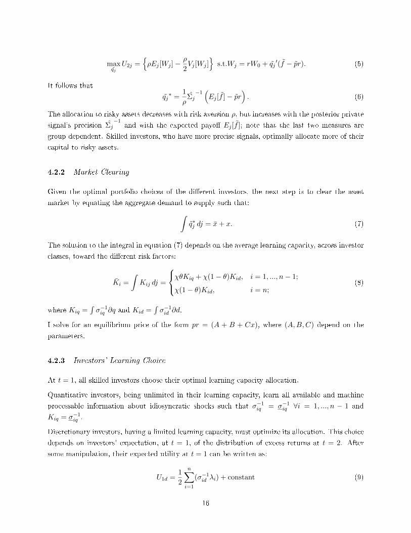
maxqj

U2j ={ρEj [Wj ]−

ρ

2Vj [Wj ]

}s.t.Wj = rW0 + qj

′(f − pr). (5)

It follows that

qj∗ =

1

ρΣj−1(Ej [f ]− pr

). (6)

The allocation to risky assets decreases with risk aversion ρ, but increases with the posterior private

signal's precision Σj−1

and with the expected payo� Ej [f ]; note that the last two measures are

group dependent. Skilled investors, who have more precise signals, optimally allocate more of their

capital to risky assets.

4.2.2 Market Clearing

Given the optimal portfolio choices of the di�erent investors, the next step is to clear the asset

market by equating the aggregate demand to supply such that:∫q∗j dj = x+ x. (7)

The solution to the integral in equation (7) depends on the average learning capacity, across investor

classes, toward the di�erent risk factors:

Ki =

∫Kij dj =

χθKiq + χ(1− θ)Kid, i = 1, ..., n− 1;

χ(1− θ)Kid, i = n;(8)

where Kiq =∫σ−1iq ∂q and Kid =

∫σ−1id ∂d.

I solve for an equilibrium price of the form pr = (A + B + Cx), where (A,B,C) depend on the

parameters.

4.2.3 Investors' Learning Choice

At t = 1, all skilled investors choose their optimal learning capacity allocation.

Quantitative investors, being unlimited in their learning capacity, learn all available and machine

processable information about idiosyncratic shocks such that σ−1iq = σ−1

iq ∀i = 1, ..., n − 1 and

Kiq = σ−1iq .

Discretionary investors, having a limited learning capacity, must optimize its allocation. This choice

depends on investors' expectation, at t = 1, of the distribution of excess returns at t = 2. After

some manipulation, their expected utility at t = 1 can be written as:

U1d =1

2

n∑i=1

(σ−1id λi) + constant (9)

16

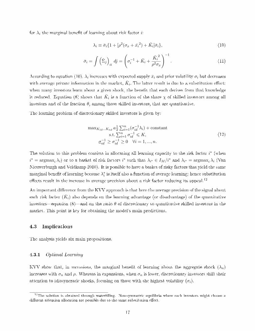
for λi the marginal bene�t of learning about risk factor i:

λi ≡ σi{1 + [ρ2(σx + xi2) + Ki]σi}, (10)

σi =

∫ (Σj

)iidj =

(σ−1i + Ki +

Ki2

ρ2σx

)−1

. (11)

According to equation (10), λi increases with expected supply xi and prior volatility σi but decreases

with average private information in the market, Ki. The latter result is due to a substitution e�ect:

when many investors learn about a given shock, the bene�t that each derives from that knowledge

is reduced. Equation (8) shows that Ki is a function of the share χ of skilled investors among all

investors and of the fraction θ, among those skilled investors, that are quantitative.

The learning problem of discretionary skilled investors is given by:

maxK1d...Knda1

2

∑ni=1(σ−1

id λi) + constant

s.t.∑n

i=1 σ−1id 6 K,

σ−1id ≥ σ

−1id ≥ 0 ∀i = 1, ..., n.

(12)

The solution to this problem consists in allocating all learning capacity to the risk factor i∗ (when

i∗ = argmaxi λi) or to a basket of risk factors i∗ such that λi∗ ∈ IM/i∗ and λi∗ = argmaxi λi (Van

Nieuwerburgh and Veldkamp 2010). It is possible to have a basket of risky factors that yield the same

marginal bene�t of learning because λ∗i is itself also a function of average learning; hence substitution

e�ects result in the increase in average precision about a risk factor reducing its appeal.12

An important di�erence from the KVV approach is that here the average precision of the signal about

each risk factor (Ki) also depends on the learning advantage (or disadvantage) of the quantitative

investors�equation (8)�and on the ratio θ of discretionary to quantitative skilled investors in the

market. This point is key for obtaining the model's main predictions.

4.3 Implications

The analysis yields six main propositions.

4.3.1 Optimal Learning

KVV show that, in recessions, the marginal bene�t of learning about the aggregate shock (λn)

increases with σn and ρ. Whereas in expansions, when σn is lower, discretionary investors shift their

attention to idiosyncratic shocks, focusing on those with the highest volatility (σi).

12The solution is obtained through water�lling. Non-symmetric equilibria where each investors might choose adi�erent attention allocation are possible due to the same substitution e�ect.

17

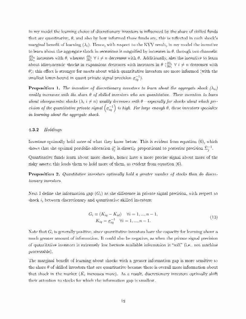
In my model the learning choice of discretionary investors is in�uenced by the share of skilled funds

that are quantitative, θ, and also by how informed those funds are, this is re�ected in each shock's

marginal bene�t of learning (λi). Hence, with respect to the KVV result, in my model the incentive

to learn about the aggregate shock in recessions is magni�ed by increases in θ, through two channels:∂λn∂σn

increases with θ, whereas ∂λi∂σi∀ i 6= n decreases with θ. Additionally, also the incentive to learn

about idiosyncratic shocks in expansions decreases with increases in θ (∂λi∂σi∀ i 6= n decreases with

θ); this e�ect is stronger for assets about which quantitative investors are more informed (with the

smallest lower-bound in quant private signal precision σ−1iq ).

Proposition 1. The incentive of discretionary investors to learn about the aggregate shock (λn)

weakly increases with the share θ of skilled investors who are quantitative. Their incentive to learn

about idiosyncratic shocks (λi i 6= n) weakly decreases with θ�especially for shocks about which pre-

cision of the quantitative private signal(σ−1iq

)is high. For large enough θ, these investors specialize

in learning about the aggregate shock.

4.3.2 Holdings

Investors optimally hold more of what they know better. This is evident from equation (6), which

shows that the optimal portfolio allocation q∗j is directly proportional to posterior precision Σ−1j .

Quantitative funds learn about more shocks, hence have a more precise signal about more of the

risky assets; this leads them to hold more of them, as evident from equation (6).

Proposition 2. Quantitative investors optimally hold a greater number of stocks than do discre-

tionary investors.

Next I de�ne the information gap (Gi) as the di�erence in private signal precision, with respect to

shock i, between discretionary and quantitative skilled investors:

Gi ≡ (Kiq −Kid) ∀i = 1, ..., n− 1,

Kiq = σ−1iq ∀i = 1, ..., n− 1.

(13)

Note that Gi is generally positive, since quantitative investors have the capacity for learning about a

much greater amount of information. It could also be negative, as when the private signal precision

of quantitative investors is extremely low because available information is �soft� (i.e., not machine

processable).

The marginal bene�t of learning about shocks with a greater information gap is more sensitive to

the share θ of skilled investors that are quantitative because there is overall more information about

that shock in the market (Ki increases more). As a result, discretionary investors optimally shift

their attention to stocks for which the information gap is smallest.

18

Proposition 3. An increase in the share θ of skilled investors that are quantitative weakly reduces

the attention allocation of discretionary investors to risk factors with a relatively greater information

gap.

4.3.3 Dispersion of Opinion

The dispersion of opinion of a representative quantitative (discretionary) investor with respect to

other quantitative (discretionary) investors is given by (derivation in Appendix D.3):

E[(qq − ¯qq) (qq − ¯qq)

′]=

1

ρ2

n−1∑i=1

σ−1iq (14)

E[(qd − ¯qd) (qd − ¯qd)

′]=

1

ρ2

n∑i=1

(σ−1id −Kid

)2f(σi, Ki, xi, ρ

)+

1

ρ2K (15)

where ¯qq =∫ [

1ρ Σq

−1(Eq[f ]− pr

)∂q], ¯qd =

∫ [1ρ Σd

−1(Ed[f ]− pr

)∂d]and f

(σi, Ki, xi, ρ

)is func-

tion of the prior volatility of shock i (σi), it's expected supply (xi), the average private signal precision

of all investors in the market about shock i (Ki) and risk aversion (ρ).13

Dispersion of opinion is determined by two e�ects. First, dispersion of opinion increases with the

total precision of private signals: the greater the total precision of private signals the more weight is

given to the heterogeneous private signals as opposed to common priors in determining posteriors.

Second, dispersion of opinion increases with the cumulative di�erence in the attention allocated by

investors to each asset with respect to the attention allocated to the same assets by the average

investor of their type. Risk tolerance magni�es both e�ects.

For quantitative investors (eq. 14) dispersion of opinion is entirely determined by the �rst e�ect; in

fact attention allocation is always symmetric among quantitative funds as they optimally learn all

available and machine processable information. For what regards discretionary investors (eq. 15),

instead, dispersion of opinion is determined by both e�ects. The �rst e�ect is represented by the

second term of equation (15): dispersion of opinion is an increasing function of total private signal

precision K. The �rst term of equation (15), instead, represents the second e�ect: the greater the

di�erence in signal precision of the investor with respect to other discretionary investors(σ−1id −Kid

),

the greater the dispersion of opinion. Discretionary investors, having a limited learning capacity,

need to choose what to learn about, due to a substitution e�ect they might choose to learn about

di�erent shocks, this increases dispersion of opinions.

Proposition 4. As long as∑n

i=1

(σ−1id −Kid

)2f(σi, Ki, xi, ρ

)>∑n−1

i=1 σ−1iq − K, dispersion of

opinion is greater among discretionary investors than among quantitative investors.

13The exact speci�cation can be found in the Appendix

19

4.3.4 Performance

An investor's risk-adjusted performance is measured as the expected excess return with respect to

the market return. Appendix E establishes that the excess return of investor j is given by

E [(Rj −RM )] = E[(q∗j − ¯q

)′ (f − pr

)]=

1

ρ

n∑i=1

[λi(Kij − Ki

)]. (16)

Expected excess returns increase with the learning advantage of investor j on the risk factors it

chooses to learn about(Kij − Ki

)> 0�and in proportion to the marginal bene�t λi of learning

about them.

With regard to the aggregate shock, quantitative investors are always at a learning disadvantage

compared with discretionary investors. With regard to idiosyncratic shocks, however, quantitative

investors generally have a learning advantage over all other investors in the market�provided Gi is

positive. When Gi is negative, their advantage is reduced but it remains positive as long as the total

share of skilled investors in the market is not too high

(σ−1iq

Kid> χ−χθ

1−χθ

):

(σ−1iq − Ki

)= [(1− χ)Kid + (1− χθ)Gi] > 0, i = 1, ..., n− 1,(

σ−1nq − Ki

)= − [Kid(χ− χθ)] < 0, i = n.

(17)

The performance of quantitative investors increases in tandem with increases in σi for i = 1, ..., n−1

thanks to the increase in the marginal bene�t of learning about those risk factors for which they

have a learning advantage. Their excess return is greatest when discretionary skilled investors choose

not to learn about the aggregate risk factor. If instead they do choose to learn about it, then the

excess return of quantitative investors declines following increases in σn. Finally, their performance

deteriorates as θ increases. The negative e�ect of an increase in θ on excess returns is greatest when

the elasticity of λi with respect to θ is high. Elasticity is increasing in∑n−1

i=1 σ−1iq , from which it

follows that excess returns deteriorate faster when each fund has higher precision of private signals.

Proposition 5. The excess returns of quantitative skilled investors increases with σi for i = 1, ..., n−1, weakly decreases in recessions (when σn increases), and always decreases with the share θ of

quantitative investors.

Greater signal precision σ−1iq acts in two opposite directions. It directly increases excess returns

thanks to the fund's greater informativeness in choosing its portfolio allocation. It indirectly de-

creases excess returns by reducing the marginal bene�t of learning about the same shocks, through

the elasticity of λi with respect to θ. This is particularly relevant as quantitative investors are uncon-

strained in their learning capacity, hence even small increases in the share of quantitative investors

θ can have a great impact on λi.

For what regards discretionary investors, when choosing to learn about the aggregate risk factor, they

earn a positive excess return if their informational advantage with respect to both unskilled investors

20

and quantitative investors (i.e., their ability to learn about the aggregate shock�the ��exibility

advantage� captured by the LHS of equation 18) is greater than their learning disadvantage with

respect to quantitative investors (i.e., owing to their smaller information capacity�the �breadth

disadvantage� captured by the RHS of equation 18). Formally,

λn [K − (χ(1− θ))Knd] > χθn−1∑i=1

[λiσ−1iq

]. (18)

When, instead, discretionary investors optimally choose to learn about idiosyncratic shocks, their

expected excess return is positive if the following (more restrictive) condition is veri�ed:

λl (K − χKld − χθGl) > χθn−1∑i 6=j

{λi

[σ−1iq

]}. (19)

In this latter case, they have a learning advantage only with respect to unskilled investors; in contrast,

they display a learning disadvantage, which is equal to the information gap Gl, with respect to

quantitative investors. Even when the information gap is negative, equation (19) represents a more

restrictive condition, since the aggregate shock is in much greater supply than any idiosyncratic

shock l that they might choose to learn about. Furthermore, an increase in the prior volatility of

the idiosyncratic shocks l, which they choose to learn about, increases their expected excess return

only if θ is su�ciently low:

θ <σ−1ld − χKld

χGl. (20)

Note that, when discretionary investors choose to learn about shocks with a smaller information

gap, their excess return rises for a wider range of θ values � potentially being always veri�ed if

focusing on shocks with . Equations (19) and (20) highlight the direct link between performance and

information gap reduction. Additionally, according to equation (20), there exist values of θ < 1 for

which discretionary investors cannot earn positive excess returns from learning about idiosyncratic

shocks. This is what leads to specialization in the aggregate shock, per Proposition 1, for high

enough values of θ.

When discretionary investors optimally choose to learn about the aggregate shock, increases in

σn always have a positive e�ect on their excess return whereas increases in σi, i = 1, . . . , n − 1,

(marginally) reduces it. This observation, together with equations (18) and (19), leads us to conclude

that discretionary skilled investors always have higher expected excess returns in recessions.

Finally, when discretionary investors choose to learn about idiosyncratic risks, their excess return

falls as θ rises. If instead they choose to learn about the aggregate risk, then increases in θ lead to

an increase in their expected excess return�provided the elasticity of λi (i− 1, . . . , n) with respect

to θ is su�ciently large�this condition is not satis�ed for shocks with a negative information gap.

Proposition 6. When discretionary investors, optimally learn about idiosyncratic shocks, their

excess return decreases with θ and with the volatility of the idiosyncratic risk factors that they ignore.

21

The excess return increases with the volatility of the shocks on which they focus but only if θ and Gl

are both low enough. When discretionary investors optimally learn about the aggregate shock, their

excess return always increases with σn and decreases with σi 6=n; it also increases with θ if the elasticity

of λi 6=n and of λn (with respect to θ) are su�ciently high.

4.3.5 Price Informativeness

We can use equation (8) to rewrite the average precision of private signals about any idiosyncratic

shock i, in terms of Gi, as follows:

Ki = χKid + χθGi. (21)

This formulation re�ects that the average private signal precision about idiosyncratic shocks amounts

to the sum of the discretionary signal's precision, χKid, and a premium (Gi > 0) for the additional

signal precision of quantitative funds, χθGi. However, the presence of quantitative investors may

end up reducing the average private signal precision about stocks for which there is little machine-

learnable information (Gi < 0).

I de�ne price informativeness as the precision of equilibrium prices, which is given by

(Σ−1p

)ii

= σ−1pi = Ki

2

ρ2σx∀i = 1, ...n. (22)

This expression is an increasing function of the average private signal precision Ki of skilled investors,

so it always increases with χ (the share of skilled investors in the market). However, the e�ect of

increases in the share θ of quantitative investors depends on the type of shock, on the extent of the

information gap, and on the state of the business cycle.

Proposition 7. An increase in θ increases (resp. decreases) the price informativeness of idiosyn-

cratic shocks with a high (resp. low) information gap. An increase in θ decreases (resp., weakly

increases) the price informativeness of the aggregate shock in recessions (resp., in expansions).

The �rst part of Proposition 7 follows from equations (21) and (22) when one considers the e�ect of θ

on the learning choice of discretionary investors. For the second part, the intuition is as follows. In

recessions, when all skilled investors are discretionary, they all learn about the aggregate shock; but

if some skilled investors are quantitative, fewer skilled investors learn about that shock, reducing

its price informativeness. In expansions, increases in θ have no e�ect on the aggregate shock's

price informativeness provided that discretionary funds choose to learn about idiosyncratic shocks.

Yet for large enough θ they optimally choose to specialize in learning about the aggregate shock

(Proposition 1), in which case its price informativeness is increased.

22

5 Empirical Analysis

5.1 Empirical Measures

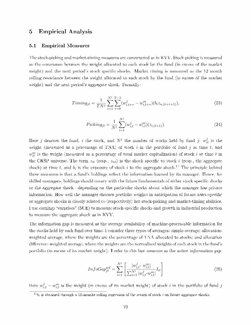
The stock-picking and market-timing measures are constructed as in KVV. Stock picking is measured

as the covariance between the weight allocated to each stock by the fund (in excess of the market

weight) and the next period's stock-speci�c shocks. Market timing is measured as the 12-month

rolling covariance between the weight allocated to each stock by the fund (in excess of the market

weight) and the next period's aggregate shock. Formally:

Timingjt =1

TN j

Nj∑i=1

T−1∑τ=0

(wji,t+τ − wmi,t+τ )(bizn,(t+τ+1)), (23)

Pickingjt =1

N j

Nj∑i=1

(wji,t − wmi,t)(zi,(t+1)). (24)

Here j denotes the fund, i the stock, and N j the number of stocks held by fund j; wjit is the

weight (measured as a percentage of TNA) of stock i in the portfolio of fund j at time t, and

wmit is the weight (measured as a percentage of total market capitalization) of stock i at time t in

the CRSP universe. The term zit (resp., znt) is the shock speci�c to stock i (resp., the aggregate

shock) at time t, and bi is the exposure of stock i to the aggregate shock.14 The principle behind

these measures is that a fund's holdings re�ect the information learned by its manager. Hence, for

skilled managers, holdings should covary with the future fundamentals of either stock-speci�c shocks

or the aggregate shock�depending on the particular shocks about which the manager has private

information. How well the manager chooses portfolio weights in anticipation of future asset-speci�c

or aggregate shocks is closely related to (respectively) her stock-picking and market-timing abilities.

I use earnings �surprises� (SUE) to measure stock-speci�c shocks and growth in industrial production

to measure the aggregate shock as in KVV.

The information gap is measured as the average availability of machine-processable information for

the stocks held by each fund over time. I consider three types of averages: simple average; allocation-

weighted average, where the weights are the percentage of TNA allocated to stocks; and allocation

di�erence�weighted average, where the weights are the normalized weights of each stock in the fund's

portfolio (in excess of its market weight). I refer to this last measure as the active information gap:

InfoGapwdjt =

Nj∑i=1

[|wji,t- wmi,t|∑Nj

i=1 |wji,t-w

mi,t|Iit

](25)

Here wji,t − wmi,t is the weight (in excess of its market weight) of stock i in the portfolio of fund j

14bi is obtained through a 12-months rolling regression of the return of stock i on future aggregate shocks.

23

at time t, and Iit is a measure of machine-processable information availability for stock i at time t.

I expect the learning e�ect to be best captured by this active information gap, since measuring

information availability for stocks that the manager decides to underweight or overweight (with

respect to the market) should better re�ect her active learning.

I construct di�erent measures of the information gap using di�erent proxies for the amount of

information available about stocks (Iit). I use the stock's size (market capitalization) and age (in

months), number of IBES end-of-period forecasts for the stock, and number of times the stock was

mentioned in Dow Jones news articles per month. The logic underlying these proxy choices is that

there should be less information available�and machine processable�about smaller and younger

stocks, which are less followed by analysts and in the media.

I measure the share θ of quantitative investors in two ways (i) as the share of assets managed by

quantitative funds relative to the total assets managed by funds in my sample (θTNA); and (ii) as

the percentage of the US stock market capitalization held by quantitative funds (θHold):

θTNAt =TNAQuantitativet

TNAQuantitativet + TNADiscretionaryt

(26)

θHoldt =

∑Qt

i=1

∑Njt

i=1 |nijt|Pit∑Nj

i=1 nitPit(27)

Here j denotes the fund, i the stock, Qt the total number of quantitative funds at time t and Njt

the number of stocks held by fund j at time t; Pit is the price of stock i at time t, nijt is the number

of shares of stock i held by fund j at time t and nit is the number of shares outstanding of stock i

at time t.

Finally, I also build two measures of dispersion of opinion. First I measure portfolio overlap (i.e.

commonality) for funds of the same group�quantitative or discretionary�as the allocation-weighted

average of the percentage of funds of the same group which hold each stock over time. For the

same reasons explained in the construction of the Active Information Gap measure, weights are the

normalized percentages of the fund's TNA allocated in each stock wjit−wmit (in excess of their marketweight):

ComonalityFjt =

Njt∑

i=1

|wjit − wmit |∑Njt

i=1 |wjit − wmit |

(FitFt

) ; (28)

for F = (Q, D), where Qt (Dt) is the total number of quantitative (discretionary) funds at time t

and Qit (Dit) is the number of quantitative (discretionary) funds who hold stock i at time t.

Second I measure holdings dispersion as the cumulative squared di�erence in the weight allocated

by each funds and the average weight allocated by funds of the same type to stocks.

24

DispersionFjt =

Njt∑

i=1

(wjit − w

Fit

)2

for F = (Q, D), where wFit is the average weight allocated by quantitative (discretionary) funds to

stock i at time t.

What I subsequently call �overcrowding� is a combination of the prevalence of quantitative funds in

the market (θ) and the commonality in their portfolios

5.2 Tests of the Model Assumptions

As a �rst step, I provide evidence in support of the model's main assumptions: that skilled quan-

titative funds specialize in learning about idiosyncratic shocks; and that the funds I classify as

discretionary adjust what they learn about, as KVV �nd.

In KVV, skilled investors are limited in information capacity but perfectly �exible in shifting their

attention from aggregate to idiosyncratic shocks. The authors �nd that skilled investors switch from

stock picking in expansions to market timing in recessions. I test for whether the skilled funds in

my sample display this switching behavior and for whether the e�ect di�ers between quantitative

and discretionary funds. For that purpose, I identify funds that are most persistently among the

top stock pickers in expansions and then check to see whether they switch to market timing in

recessions. Finally, I check for whether any of the fund classes specializes in either stock picking or

market timing across phases of the business cycle.

I begin by constructing the market-timing and stock-picking measures described in Section (5.1).

Next I identify all observations belonging to the top quartile of the market-timing distribution in

recessions or of the stock-picking distribution in expansions (i.e., the high-ability sample). Finally,

for each fund I calculate how frequently members of this high-ability sample exhibit market-timing

ability in recessions or stock-picking ability in expansions. Frequency is measured as the number of

months (relative to their respective lifetimes) that funds are among the top timers or the top pickers.

Thus TopP ickersE and TopT imersR refer to the top quartile of funds that most frequently display,

respectively, high stock-picking ability in expansions and high market-timing ability in recessions.

I then run the following regressions, where (as before) Quant j is a dummy set equal to 1 if the fund

is quantitative (and to 0 otherwise):

Timingjt = α+β1TopP ickersEj +β2Quantj+β3TopP ickers

Ej ∗Quantj+γXjt+εt|Recession; (29)

Pickingjt = α+β7TopP ickersEj +β8Quantj+β9TopP ickers

Ej ∗Quantj+γXjt+εt|Recession. (30)

25

Timingjt = α+β4TopT imersRj +β5Quantj+β6TopT imers

Rj ∗Quantj+γXjt+εt|Expansion; (31)

Recessions and expansions are identi�ed using NBER business cycle dates. The term Xjt represents

a series of fund-speci�c control variables previously described (see Table 1 for details).

Equation (29) tests whether high-ability funds switch from stock picking in expansions to market

timing in recessions. Consistently with the KVV results, I �nd that the funds with high stock-

picking ability in expansions also have high market-timing ability in recessions (β1 = 0.454 > 0).

For quantitative funds, however, this e�ect cancels (β3 = −0.621 < −β1): quantitative funds do

not optimally switch between stock picking and market timing across the business cycle (Model 1

in Table 5).

Equations (30) and (31) test for whether some funds specialize in, respectively, stock picking and

market timing across the business cycle. In line with the model's assumptions, I �nd that quantitative

funds among the top stock pickers in expansions are also among top stock pickers in recessions

(β8 = 0.356 > 0; β9 = 0.248 > 0); these results con�rm that quantitative funds specialize in

learning about idiosyncratic shocks (Model 2 in Table 5). Finally no funds are persistently among

the top market timers across business cycle phases (i.e., neither β4 nor β6 is signi�cant). This �nding

con�rms the hypothesis that, among equity mutual funds, none specializes in market timing (Model 3

in Table 5).

5.3 Market-Timing and Stock-Picking

Turning to the model's main predictions, I �rst test Proposition 1: as the share of quantitative

investors rises, the incentive of discretionary investors to learn about the aggregate shock in recessions

increases; conversely, their incentive to learn about idiosyncratic shocks in expansions decreases.

I test these predictions via the measures (described in Section 5.1) of market timing, stock picking,

and share of quantitative funds. Particularly the share of quantitative funds is measured as a

proportion of assets managed (θTNA) and as the percentage of the US market capitalization held by

quantitative funds (θHold). These two measures are used in running the following regressions:

Pickingjt = α+ β1NBERt + β2θTypet + γXjt + εt| j = d

T imingjt = α+ β3NBERt + β4θTypet + γXjt + εt| j = d

whereNBERt is an indicator variable which identi�es recession periods, θType (for Type = (TNA, Hold))

is the proxy for θ and Xj are a series of fund speci�c control variables (The same as speci�ed in

table 1).

I �rst con�rm KVV's �nding that the stock-picking ability of discretionary investors is greatest in

expansions (β1 < 0) whereas their market-timing ability is greatest in recessions (β3 > 0).

26

I also �nd evidence in favor of Proposition 1. Using θTNA as a proxy for θ, the coe�cient β2 = −0.143

is negative and signi�cant at the 1% level: a 1% increase in θ reduces the stock-picking ability of

discretionary investors by 8.5% of a standard deviation. Conversely, β4 = 0.149 is positive and

signi�cant at the 1% level: a 1% increase in θ increases the market timing ability of discretionary

investors by 14% of a standard deviation (Models 1�2 of Table 8).

A concern is reverse causality if θTNA proxies for out�ows from discretionary funds. For that to be

the case, we would �rst need to believe in a direct causality between out�ows and learning ability,

additionally for the signs to be correct it would imply that out�ows impact stock picking positively

and market timing negatively, this seems implausible. To further alleviate this concern, I repeat the

analysis using θHold (eq. 27), which, despite not being completely independent from fund �ows, is

not directly related to discretionary fund �ows. In fact funds might change their investment in the

stock market to hold more cash or invest in other non-equity products. I obtain similar �ndings

(Table 8, Models 3�4). Results are robust controlling for the total US stock market capitalization

held by discretionary funds.

5.4 Portfolio Diversi�cation

Next I test Proposition 2, which states that quantitative funds are expected to hold signi�cantly

more stocks than do discretionary funds.

As reported in Table 6, quantitative funds hold about double the number of stocks held by discre-

tionary funds ('117+108 vs. 117). Results are robust to controlling for the amount of cash held,

the size of funds, and various other fund characteristics. Moreover, the distribution of the number

of stocks held by discretionary funds is quite concentrated, with most observations falling between

10 and 100 stocks. Quantitative funds exhibit a more dispersed distribution, and a sizable number

of them hold as many as 1,000 stocks. The distribution of the number of holdings seems not to vary

with recessions and expansions (Figure 12). 15

The greater portfolio diversi�cation among quantitative funds is re�ected in their marginally lower

portfolio risk, as shown in Table 7. The �rst two columns consider the 12- and 36-month rolling

volatility of fund returns. Compared with discretionary funds, quantitative funds exhibit (on average)

2% lower return volatility; and in recessions, volatility increases 8% less. In columns 3�8 of the table,

portfolio risk is de�ned as the 12- and 36-month rolling idiosyncratic volatility of fund returns.

Idiosyncratic volatility is measured as the volatility of the residual of a regression of excess fund

returns on (i) the excess return on the market, (ii) the Fama�French three-factor model, and (iii) the

Carhart four-factor model (CAR). I �nd that quantitative funds' returns display between 8.3% (for

36-month rolling CAPM) and 15.6% (for 12-month rolling CAR) less idiosyncratic volatility than

discretionary funds.

15Quantitative funds hold a signi�cantly larger number of stocks than discretionary funds also when using quantileregressions based on the distribution of the number of holdings � results available upon request

27

5.5 Information Gap

Proposition 3 indicates the presence of cross-sectional di�erences in the learning of discretionary

and quantitative investors; in particular, skilled discretionary investors should shift their attention

to stocks for which less information is learnable/available in order to reduce their information gap

with respect to quantitative investors. For each proxy I construct the simple average, the allocation-

weighted average, and the active information gap (equation 25) for the stocks held by each fund

over time. I then regress the information gap proxies on dummies that identify recession peri-

ods and discretionary funds, an interaction between those two dummies, and various fund-speci�c

characteristics:

InfoGapjt = α+ β1NBERt + β2Discretionaryj + β3NBERt ×Quantj + γXjt + εt;

here NBERt is a dummy variable identifying recessions, Discretionaryj is a dummy variable that

identi�es discretionary funds, and Xjt represents the fund-speci�c control variables described in

Table 1.

I expect β2 to be negative and signi�cant, which would indicate that (on average) discretionary

funds hold stocks with a smaller information gap. Mutual fund returns are evaluated against a

benchmark, so one should expect mutual fund managers to hold not only stocks about which they

actively learn but also a combination of other stocks that replicate the benchmark. In that case,

active mutual fund managers can be expected to underweight or overweight�with respect to that

benchmark�those stocks for which they have (through learning) formed a directional view. That

dynamic could bias upward the simple average measure of information gap when stocks held as part

of the benchmark are large ones for which a substantial amount of information is available. This

measure should have an even greater upward bias for discretionary funds given that, as shown in

Section 5.4, they hold fewer stocks. For that reason I expect the simple average measure of the

information gap to fare the worst at capturing this e�ect. The allocation-weighted average should

mitigate such an upward bias, but the best measure should be the active information gap because it

isolates those stocks for which the manager's portfolio allocation deviates from the benchmark, an

indication of active learning.

I �nd that discretionary funds hold 17% smaller stocks (Model 3 in Table 9). As expected, the

e�ect is not signi�cant for the simple average measure of the information gap (Model 1) but is

signi�cant when either the allocation-weighted average or the active information gap (Models 2

and 3, respectively) is used. In addition, discretionary funds hold stocks that are 11% younger

(Model 5 in Table 10); this e�ect persists even after controlling for the average stock size, which

indicates that stock age is not just a proxy for stock size. The age e�ect is signi�cant for all measures,

but it is stronger when the allocation-weighted average or the active information gap are used.

Discretionary funds also hold stocks that have 11% fewer mentions in Dow Jones media (Model 5

of Table 11). This e�ect is not signi�cant when I use the simple average but is signi�cant under

28

the allocation-weighted average�though only at the 10% level when controlling for average market

capitalization of the stocks held. As expected, the e�ect is strongest (11% fewer mentions; signi�cant

at the 1% level) under the active information gap measure, even after controlling for the average

market capitalization of the stocks held. The e�ect of discretionary funds on the information gap, as

measured by the number of analyst forecasts, is negative but not signi�cant (Model 5 in Table 12).

Finally, we con�rm that discretionary funds earn a marginally higher premium when investing in

stocks characterized by a smaller information gap (Table 13).

5.6 Dispersion of Opinion

Proposition 4 states that there should be a greater dispersion of opinion among discretionary funds

than among quantitative funds. I test this proposition using the measures for commonality and

dispersion described in section 5.1. The intuition being that a greater dispersion of opinion among

investors about assets' payo� should lead to more diversi�ed hidings. Figure 13 displays the dis-

tribution of commonality (Panel 1) and holdings dispersion (Panel 2) among quantitative and dis-

cretionary funds over the entire period. Quantitative funds display a lower dispersion (more con-

centrated distribution) and higher holdings commonality than discretionary funds. Additionally

we can clearly see a two-picked distribution for the commonality measure, particularly pronounced

for quantitative funds, indicating that funds polarize between a low and high common portfolio

ownership, which for quantitative funds picks at roughly 6% and 20%. Table 14 further shows the

statistical signi�cance of this di�erence. Model 1 shows that dispersion of holdings is signi�cantly

about 30% greater for discretionary funds than quantitative funds. Whereas Model 2 shows that

holdings commonality is signi�cantly lower for discretionary funds (9% vs 14.79%).

5.7 Performance

Propositions 5 and 6 concern the relative performance of quantitative and discretionary funds

across the business cycle. In KVV the authors report a signi�cantly higher performance in re-

cessions�34 basis points when measured by 12-month rolling CAPM alphas�and the premium

was greatest for funds that shifted from market timing in recessions to stock picking in expansions

(their period of analysis was 1980�2005). When replicating that result using my data sample (for

the period 1999�2015), I �nd a lower recession premium (28 bp) if I do not control for the Quantj

dummy (Model 1 in Table 15). Yet when controlling for the presence of quantitative funds, the

recession premium of discretionary investors is recovered (31.4 bp), and it emerges that quantitative

investors display signi�cantly lower performance: earning 15.7 bp less than discretionary investors

in recessions (Model 2 in Table 15). Results are robust to incorporating various fund-level controls:

age, size, turnover rate, expenses ratio, net �ows, fund �ow volatility, fund loads, and exposure to

the size, value, and momentum factors (Model 3 in Table 15). Results persist also when computing

performance as the 36-month rolling CAPM alpha, despite the recession's e�ect being weaker under

that criterion (Model 4 in Table 15).

29

Similar results are obtained when performance is computed using the Fama�French three-factor

model (Table 16) and the Carhart four-factor model (Table 17); these results are in line with Propo-

sitions 5 and 6. With respect to the Fama�French three-factor 12-month rolling alphas, the perfor-

mance premium is not signi�cant absent controlling for the di�erent performance of quantitative

and discretionary funds. A recession premium of 8.56 bp is recovered for discretionary funds when

the regression includes the Quant j dummy, in which case quantitative funds are found to return (on

average) 9.51 bp less than discretionary investors in recessions. Results are robust to adding fund-

speci�c control variables and using 36-month rolling alphas. When using the Carhart four-factor

model, we observe a recession premium of 4.26 bp that is signi�cant only when using 36-month

rolling alphas; in contrast, the negative premium of quantitative funds in recession�which ranges

from 6.04 bp to 9.01 bp�is signi�cant under all model speci�cations.

Regarding the performance of quantitative funds, Proposition 5 highlights di�erent e�ects that go

in opposite directions. First, the learning behavior of quantitative funds induces them to make

more informed trades in expansions. Second, the greater amount of information learned, leads to

greater portfolio diversi�cation, as shown in Section 5.4. This should produce better risk-adjusted

performance, but at the same time it should prevent them from being greatly exposed to any single

idiosyncratic shock from which they could pro�t. Finally performance deteriorates more the greater

is the share of quantitative investors in the market and information availability (�overcrowding�).

Overcrowding is exacerbated when funds hold similar portfolios.

In order to disentangle these di�erent e�ects, I have looked at the two dimensions of �overcrowding�:

holdings commonality and the rise in the share of quantitative funds over time. Particularly the

greater overlap in the quantitative portfolios holding leads �overcrowding� to have a stronger impact

on the performance of quantitative funds (Figure 13). In order to further explore the e�ect of

overcrowding over time I have built two additional dummy variables: E1 and E2 which identify

respectively the expansion period prior to the millennial recession (Dec 1999�Mar 2001) and the

expansion period in between the two recessions in my sample (Dec 2001�Nov 2007) . The regression

speci�cations also contain a recessions dummy, hence all coe�cients are interpreted relative to the

expansion post subprime crisis:

αQjt = γ + γ1E1t + γ2E2t + γ3NBERt + εt (32)

where αjt is the 12-months rolling CAPM, Fama-French 3-factor and Carhart 4-factor alpha.

Models 1,2 and 3 of Table 18 clearly show that the expansion premium of quantitative funds has

been decreasing over time. In the CAPM speci�cation, the per-millennial recession (E1) expansion

displays a premium of 79.8bp more than the post-subprime expansion, the premium fuhrer decrease

to 12.1bp for the per-subprime second expansion. In the CAPM speci�cation a recession premium

of 20.7bp also �gures but this becomes insigni�cant when using the 3-factor or 4-factor models. For

the 3-factors and 4-factors models the E1 premium is of 40.4bp and 46.0bp respectively, while the E2

expansion doesn't seem to be signi�cantly di�erent from the post-subprime one. Model 4 of Table

30

18 runs the same speci�cation as in equation (32) but using the 12-months rolling Sharpe ratio as

independent variable. By doing so I �nd a signi�cantly positive Sharpe Ratio in expansions (25.1bp),

while a negative Sharpe ratio emerges for E1 (58.1bp�signi�cant at the 10% level). Additionally

recessions display a signi�cantly negative Sharpe ratio (53.2bp). This suggests that quantitative

funds might have countered the worsening in performance due to overcrowding with progressively

better risk management practices. Finally Models 5 and 6 of Table 18 show that quantitative funds

with a smaller commonality in holdings tend to perform better. The result is strong both using the

commonality measure (Model 5) and a commonality dummy, which takes a value of 1 to identify

those funds who display commonality above the median for their group (Model 6).

6 Conclusion

This paper demonstrates that the distinction between quantitative and discretionary funds is ex-

tremely relevant. The key to understanding what distinguishes them lies in their respective learning

behaviors and in the relative share of quantitative to discretionary funds in the market. The current

status quo in quantitative modeling determines a trade-o� between information quantity and �exi-

bility, which allows human traders to carve a niche in which they can maintain signi�cantly greater

(risk-adjusted) performance in recessions. Quantitative investors, though, display better portfolio

diversi�cation and risk management throughout the business cycle. A very important concept in

understanding the relative performance of quantitative and discretionary funds is overcrowding. As

the amount of information progressively incorporated in prices increases, the ability of investors

to maintain high risk adjusted performance deteriorates. This is particularly relevant as quantita-

tive investors are unconstrained in their learning capacity, hence even small increases in the share

of quantitative investors in the market can have a great impact on performance. Funds who are

able to achieve a lower overlap of their portfolio with respect to their peers are able to maintain

a competitive edge. It is important to understand this interaction because it could foretell future

developments. Indeed, increases in the availability and use of big data could well accentuate the

breadth advantages of quantitative funds but it could also worsen the overcrowding e�ect, unless

funds are able to maintain heterogeneity in their portfolio allocations. At the same time, recent de-

velopments in arti�cial intelligence�in particular, deep learning neural networks�could provide a

foundation for overcoming the limited �exibility of current quantitative models. This paper provides

a framework to start thinking about these issues.

31

References

Admati, Anat R. 1985. �A Noisy Rational Expectations Equilibrium for MultiAsset Securities Mar-

kets�. Econometrica 53:629�657.

Ahmed, Parvez, and Sudhir Nanda. 2005. �Performance of enhanced index and quantitative equity

funds�. Financial Review 40 (4): 459�479.

Anton, Miguel, and Christopher Polk. 2014. �Connected stocks�. The Journal of Finance 69 (3):

1099�1127.

Bershova, Nataliya, and Dmitry Rakhlin. 2013. �High-frequency trading and long-term investors: a

view from the buy-side�. Journal of Investment Strategies 2 (2): 25�69.

Boehmer, Ekkehart, Kingsley Y. L. Fong, and Juan Wu. 2015. �International evidence on algorithmic

trading�. Available at SSRN.

Brogaard, Jonathan, Terrence Hendershott, and Ryan Riordan. 2014. �High-frequency trading and

price discovery�. Review of Financial Studies 27 (8): 2267�2306.

Campbell, John Y., et al. 2001. �Have individual stocks become more volatile? An empirical explo-

ration of idiosyncratic risk�. The Journal of Finance 56 (1): 1�43.

Carrion, Allen. 2013. �Very fast money: High-frequency trading on the NASDAQ�. Journal of Fi-

nancial Markets 16 (4): 680�711.

Casey, Quirk, and Associates. 2005. �The Geeks Shall Inherit the Earth? Quantitative Managers'

Recent Edge�. Research Insight.

Chaboud, Alain P., et al. 2014. �Rise of the machines: Algorithmic trading in the foreign exchange

market�. The Journal of Finance 69 (5): 2045�2084.

Chan, Yeung L., and Leonid Kogan. 2002. �Catching up with the Jonases: Heterogeneous preferences

and the dynamics of asset prices�. Journal of Political Economy 110 (6): 1255�1285.

Chui, Michael, James Manyika, and Mehdi Miremadi. 2016. Where machines could replace hu-

man and where they can't (yet). McKinsey Quarterly. http://www.mckinsey.com/business-

functions/digital-mckinsey/our-insights/where-machines-could-replace-humans-and-

where-they-cant-yet.

Cochrane, John H. 2006. �Financial Markets and the Real Economy�. In International Library of

Critical Writings in Financial Economics, vol. 18. London: Edward Elgar.

Conrad, Jennifer, Sunil Wahal, and Jin Xiang. 2015. �High-frequency quoting, trading, and the

e�ciency of prices�. Journal of Financial Economics 16 (2): 271�291.

Cover, Thomas M., and Joy A. Thomas. 1991. Elements of Information Theory. First edn. John

Wiley / Sons, New York, New York.

De Souza, Andre, and Anthony W. Lynch. 2012. �Does mutual fund performance vary over the

business cycle?� National Bureau of Economic Research, no. w18137.

32

Dumas, Bernard. 1989. �Two-Person dynamic equilibrium in the capital markets�. Review of Finan-

cial Studies 2 (2): 157�188.

Elton, Edwin J., Martin J. Gruber, and Christopher R. Blake. 2001. �A �rst look at the accuracy

of the CRSP mutual fund database and a comparison of the CRSP and Morningstar mutual fund

databases�. The Journal of Finance 56 (6): 2415�2430.

Engle, R., and J. Rangel. 2008. �The Spline-GARCH Model for low-Frequency Volatility and Its

Global Macroeconomic Causes�. Review of Financial Studies 21 (3): 1187�1222.

Fabozzi, Frank J., and Sergio M. Focardi. 2009. �Black swans and white eagles: on mathematics and

�nance�. Mathematical Methods of Operations Research 69 (3): 379�394.

Fabozzi, Frank J., Sergio M. Focardi, and Caroline L. Jonas. 2008a. �Challenges in Quantitative

Equity Management�. (corrected July 2008), Research Foundation of CFA Institute Publications:

1�110.

� . 2008b. �On the challenges in quantitative equity management�. Quantitative Finance 8 (7): 649�

665.

� . 2007. �Trends in quantitative equity management: survey results�. Quantitative Finance 7 (2):

115�122.

Fama, Eugene F., and Kenneth R. French. 1989. �Business Conditions and Expected Returns on

Stocks and Bonds�. Journal of Financial Economics 25 (1): 23�49.

Fang, Lily H., Joel Peress, and Lu Zheng. 2014. �Does media coverage of stocks a�ect mutual funds'

trading and performance?� Review of Financial Studies 27 (12): 3441�3466.

Garleanu, Nicolae, and Stavros Panageas. 2015. �Young, old, conservative, and bold: The implications

of heterogeneity and �nite lives for asset pricing�. Journal of Political Economy 123 (3): 670�685.

Glasserman, Paul, and Harry Mamaysky. 2016. �Market E�ciency with Micro and Macro Informa-

tion�. Available at SSRN.

Glode, Vincent. 2011. �Why mutual funds underperform�. Journal of Financial Economics 99 (3):

546�559.

Greenwood, Robin, and David Thesmar. 2011. �Stock price fragility�. Journal of Financial Economics

102 (3): 471�490.

Grossman, Sanford J., and Joseph E. Stiglitz. 1980. �On the impossibility of informationally e�cient

markets�. The American economic review 70 (3): 393�408.

Hamilton, James D., and Gang Lin. 1996. �Stock Market Volatility and the Business Cycle�. Journal

of Applied EconometricsJournal of Applied Econometrics 11 (5): 573�539.

Harvey, Campbell, et al. 2017. �Man vs. Machine: Comparing Discretionary and Systematic Hedge

Fund Performance�. The Journal of Portfolio Management 43 (4): 55�69.

Hasbrouck, Joel, and Gideon Saar. 2013. �Low-latency trading�. Journal of Financial Markets 16

(4): 646�679.

33

Kacperczyk, Marcin, Clemens Sialm, and Lu Zheng. 2008. �Unobserved actions of mutual funds�.

Review of Financial Studies 21 (6): 2379�2416.

Kacperczyk, Marcin, Stijn Van Nieuwerburgh, and Laura Veldkamp. 2016. �A Rational Theory of

Mutual Funds Attention Allocation�. Econometrica 84 (2): 571�626.

� . 2014. �Time Varying Fund Manager Skill�. The Journal of Finance 69 (4): 1455�1484.

Khandani, Amir E., and Andrew W. Lo. 2011. �What happened to the quants in August 2007?

Evidence from factors and transactions data�. Journal of Financial Markets 14 (1): 1�46.

Kohavi, Ron. 1995. �A study of cross-validation and bootstrap for accuracy estimation and model

selection�. Ijcai 14 (2).

Kosowski, Robert. 2011. �Do mutual funds perform when it matters most to investors? US mutual

fund performance and risk in recessions and expansions�. The Quarterly Journal of Finance 1 (3):

607�664.

Lettau, Martin, and Sydney C. Ludvigson. 2010. �Measuring and modeling variation in the risk-

return tradeo��. In Handbook of Financial Econometrics. Ait-Sahalia / Hansen, L. P. Amsterdam:

North-Holland.

Ludvigson, Sydney C., and Serena Ng. 2009. �Macro factors in bond risk premia�. Review of Financial

Studies 22 (12): 5027�5067.

Ma¢kowiak, Bartosz, and Mirko Wiederholt. 2015. �Business cycle dynamics under rational inatten-

tion�. The Review of Economic Studies: rdv027.

� . 2009. �Optimal sticky prices under rational inattention�. The American Economic Review 99 (3):

769�803.

Malinova, Katya, Andreas Park, and Ryan Riordan. 2016. �Do retail traders su�er from high fre-

quency traders?� Available at SSRN.

Menkveld, Albert J. 2016. �The economics of high-frequency trading: Taking stock�. Annual Review

of Financial Economics 8:1�24.

Riordan, Ryan, and Adreas Storkenmaier. 2012. �Latency, liquidity, and price discovery�. Journal of

Financial Markets 15 (4): 416�437.

Shkilko, Andriy, and Konstantin Sokolov. 2016. �Every cloud has a silver lining: Fast trading, mi-

crowave connectivity and trading costs�. Available at SSRN.

Sims, Christopher A. 2003. �Implications of rational inattention�. Journal of monetary Economics

50 (3): 665�690.

� . 2006. �Rational inattention: Beyond the linear-quadratic case�. The American economic review

96 (2): 158�163.

Stoll, Hans R. 2014. �High speed equities trading: 1993-2012, Asia-Paci�c�. Journal of Financial

Studies 43 (6): 767�797.

34

Van Nieuwerburgh, Stijn, and Laura Veldkamp. 2010. �Information acquisition and under-diversi�cation�.

The Review of Economic Studies 77 (2): 779�805.

Varma, Sudhir, and Richard Simon. 2006. �Bias in error estimation when using cross-validation for

model selection�. BMC bioinformatics 7 (1): 91.

Wachter, J.A. 2002. �Portfolio and Consumption Decisions under Mean-Reverting Returns: An Exact

Solution for Complete Markets�. The Journal of Financial and Quantitative Analysis 37 (1): 63�

91.

World Economic Forum. 2015. �The future of �nancial services�. World Economic Forum, An In-

dustry Project of the Financial Services Community. Prepared in collaboration with Deloitte.

http://www3.weforum.org/docs/WEF_The_future__of_financial_services.pdf.

35

APPENDIX

A Fund Classi�cation

A.1 Nested Cross-Validation

Nested Cross-Validation is used in order to select the most accurate model, given the available

training sample, simultaneously choosing the best algorithm and the best set of parameters. The

procedure is an extension of a k-fold cross-validation method with a grid search.

K-fold cross-validation is used in order to assess a given algorithm's performance (intended as the

percentage of samples correctly classi�ed). The method consists in splitting the training sample

randomly into k folds without replacement. Subsequently (k − 1) of these folds are used to train

the machine learning algorithm and one fold is used to test its performance. The procedure is

then repeated k times so to obtain k performance estimates, the �nal performance measure is the

average of the k estimates. This procedure allows to obtain a measure that is less dependent on

how the training sample is divided between validation and test sets and limits the possibility of

having a biased performance measures due to under�tting or over�tting. This method is generally

combined with a grid search in order to select the best combination of parameters for a given

machine learning algorithm. The procedure is quite simple and consists in repeating the k-fold

cross-validation procedure for all possible combination of parameters in a grid, the set of parameters

which yields the highest k-fold cross-validation performance is then selected.

Nested-cross validation is an extension of the above procedure with an added k-fold layer, as illus-

trated in Figure 3. In the outer loop the training sample is split into the training and test folds, as

described above. The added inner loop is a k-fold layer applied to each training fold and used to

select the best set of parameters. The procedure is then repeated in combination with a grid search

for di�erent machine learning algorithms and the most accurate one is chosen. Varma and Simon

2006 calculate that the true error of the estimate is almost unbiased relative to the test set when

nested cross-validation is used.

Given the small sample nature of the application discussed in this paper, strati�ed k-fold cross vali-

dation is used throughout the procedure in order to improve estimates (Kohavi 1995). Strati�cation

consists in preserving the class proportions in each fold to ensure that all folds are representative of

the class proportions in the training dataset.

A.2 Random Forest

The random forest is a type of decision tree classi�er, speci�cally it is an ensemble of decision trees,

whose �nal classi�cation is decided by majority voting.

36

Binary decision tree classi�ers consist in breaking down the data into subsets by asking a series of

questions inferred from the training sample. More speci�cally at the root of the tree the algorithm

computes the information gain obtained by splitting the data according to each feature in the features

matrix. The feature that determines the highest information gain is chosen and the training sample

is split into two sub-samples according to the chosen feature. The second iteration includes two

nodes, for each of the two nodes the same procedure is repeated and so on iteratively until all

samples at each node belong to the same class. In order to avoid over�tting a limit to the maximum

depth of the tree is usually set � this is referred to as pruning. In a binary tree the information gain

which is maximized at every split is de�ned as the di�erence in impurity between the parent node

and the two children nodes:

IG(Nodeparent, f) = I(Nodeparent)−Nleft

NpI(Nodeleftchild)−

Nleft

NpI(Noderightchild)

where IG(Nodeparent, f) is the information gain at the parent node for feature f and Np, Nright and

Nleft are the number of samples in the parent node, the right and the left children nodes respectively.

The impurity measure I(node) used in this paper is entropy:

I(node) = −class∑i=1

p(i|node)log2p(i|node)

where p(i|node) is the proportion of samples in the node that belong to class i � hence entropy is 0

when all samples in a node belong to the same class and it is maximum when samples are uniformly

distributed across classes.

In order to better illustrate the procedure Figure 4 displays an example of a single decision tree run on

the 200 pre-classi�ed prospectuses with maximum tree depth set to 3 and entropy impurity measure.

We observe that quantit (the stemmed version of quantitative, quantitatively, ...) is selected as the

most informative feature at the �rst node. Some of the features selected in subsequent nodes are

also quite interpretable (e.g. disciplin, proprietari) but many are not. This might be due to the fact

that a single decision tree is likely to over�t the training sample, making its in-sample accuracy very

high but its out-of-sample performance very poor.

A way to minimize these generalization and over�tting issues it to employ a random forest. The

random forest can be described in four steps:

1. Randomly choose a sample of size n from the training sample with replacement

2. Grow a decision tree from the selected sample. At each node:

(a) Randomly select f features from the features matrix without replacement

(b) Among the selected subset of features (f) choose the one that maximizes the information

gain and split the node according to that feature

37

3. Repeat the above 2 steps k times and record the classi�cation of each item in the training

sample by each of the k trees

4. Use majority voting to assign a �nal classi�cation to each item in the training sample

The key parameter to be chosen is the number of trees in the random forest (k), the larger the

number the better the prediction but the higher the computational burden. In this application 1000

trees were used.

A.3 Word Search

The words utilized in the �word search� of fund behaviors in mutual fund prospectuses is summarized

as follows (variations of each word/clause were considered):

1. activeTrading - active trading, actively trade, actively traded, actively and frequently traded,

actively managed

2. frequentTrading - short-term trading, short-term trade, shortterm trade, frequent trading,

frequently traded, frequently and actively traded, frequent and active trading

3. shortsell - short-selling, short-sell, selling securities short, sell securities short, selling short,

short portfolio, sell short, short-sale, sold short, shorting, sells, short position, 110/10, 115/15,

130/30, 150/50, long-short, long/short strategy, short positions, short position, sells a security

short

4. trendFollowing - behavioral, sentiment, momentum, behavior factors, momentum/sentiment,

technical analysis, chart patterns, uptrend, up-trending, stock price up-trending, price down-

trend, down-trending, relative price down-trending, price changes in trend direction, analyzing

long-term relative price trends, analyzing price trends, analysis of price trends, investor psy-

chology, long term trends, relative price movement

B Useful Derivations

1. The sensitivity of the marginal bene�t of learning about risk factor i with respect to its

expected supply is positive and is given by:

∂λi∂x2

i

=∂

∂x2i

[σi + σi

2ρ2σx + σi2ρ2σxx

2i + σi

2Ki

]= σi

2ρ2 > 0 (33)

2. The sensitivity of the marginal bene�t of learning about risk factor i with respect to its

volatility is positive and is given by:

∂λi∂σi

={

1 + 2[ρ2(σx + x2

i

)+ Ki

]σi}( σi

σi

)2

> 0 (34)

38

This positive e�ect is decreasing in the share of skilled funds who use quantitative strategies

θ for i = 1, ..., n− 1, for shocks with a positive information gap:

∂λi∂σi∂θ

= −2χ(σ−1ηi − Kid

)σi

{3σi[ρ2(σx + x2

i

)+ Ki

]( 2Ki

ρ2σx+ 1

)+

2Ki

ρ2σx

}(σiσi

)2

(35)

It is instead always increasing for i = n, when σ−1ηi = 0:

∂λi∂σi∂θ

= 2χKidσi

{3σi[ρ2(σx + x2

i

)+ Ki

]( 2Ki

ρ2σx+ 1

)+

2Ki

ρ2σx

}(σiσi

)2

(36)

3. The sensitivity of the marginal bene�t of learning about risk factor i with respect to the

average precision of private signals about i (Ki) is negative and is given by

∂λi∂Ki

= −2σi

{Ki

ρ2σx+ σi

[ρ2(σx + x2

i

)+ Ki

]( 2Ki

ρ2σx+ 1

)}< 0 (37)

4. The sensitivity of the marginal bene�t of learning about risk factor i with respect to the share

of skilled investors using quantitative strategies is given by:

∂λi∂θ

= −2χ(σ−1ηi −Kid

)σ2i

{Ki

ρ2σx

[1 + 2σi

[ρ2(σx + x2

i

)+ Ki

]]+ σi

[ρ2(σx + x2

i

)+ Ki

]}(38)

Exploring the sign of the derivative in equation 38 we can see that:∂λi∂θ < 0 i = 1, ..., n− 1 and Gi > 0

∂λi∂θ > 0 i = 1, ..., n− 1 and Gi < 0

∂λi∂θ > 0 i = n

(39)

For i = n, σ−1ηn = 0, for all other risk factors instead we have that a rise in σ−1

ηi reduces the

positive e�ect (Gi < 0) or increases the negative (Gi < 0) e�ect of θ on λi:

∂λi

∂θ∂σ−1ηi

= −2χσ2i {χθ

(σ−1ηi −Kid

) [ 1

ρ2σx+ σi +

2σiρ2σx

[2Ki + ρ2

(σx + x2

i

)]]+

+Ki

ρ2σx+ σiKi + σiρ

2(σx + x2

i

)} < 0

(40)

A similar reasoning applies for increases in the information gap Gi:

∂λi∂θ∂Gi

= −2χσ2i {χθGi

[1

ρ2σx+ σi +

2σiρ2σx

[2Ki + ρ2

(σx + x2

i

)]]+

+Ki

ρ2σx+ σiKi + σiρ

2(σx + x2

i

)}+

Ki

ρ2σx+ σiKi + σiρ

2(σx + x2

i

)} < 0

(41)

Finally also increases in the expected supply of risk factor i reduces the positive e�ect (Gi < 0)

or increases the negative (Gi < 0) e�ect of θ on λi:

∂λi∂θ∂x2

i

= −2χ(σ−1ηi −Kid

)σ3i

( ¯2Ki

σx+ ρ2

)(42)

39

Exploring the sign of the derivative in equation 42 we can see that:∂λi∂θ∂x2

i< 0 i = 1, ..., n− 1 and Gi > 0

∂λi∂θ∂x2

i> 0 i = 1, ..., n− 1 and Gi < 0

∂λi∂θ∂x2

i> 0 i = n

5. The elasticities of λi 6=n and λn with respect to θ are given by:

eλi6=n,θ = −∂λi 6=n∂θ

θ

λi 6=n> 0; eλn,θ =

∂λn∂θ

θ

λn> 0 (43)

C Model Solution

C.1 Market-clearing

The model is solved in terms of synthetic assets only a�ected by one risk-factor each, after the model

has been solved, we can map the results back from synthetic assets to real ones.

Solving for the market clearing condition we obtain that:

A = Γ−1µ− ρ¯

Σx; B = I − ΣΣ−1; C = −ρΣ

(I − 1

ρ2σxΣ−1η

)

pr = Γ−1µ+¯

Σ

[(Σ−1 − Σ−1

)z − ρ(x− x)− 1

ρ2σxΣ−1η x

]Where:

Σ−1 = Σ−1 + Σ−1p + Σ−1

η ; Σ−1P =

(σxB

−1CC ′B−1′)−1

=1

ρ2σxΣ−1′η Σ−1

η

See Admati 1985 and Kacperczyk, Van Nieuwerburgh, and Veldkamp 2016 for more details on the

derivation.

C.2 Discretionary learning choice

The discretionary investors' optimal learning problem is obtained by solving the following system of

equations: U1d = E1

[ρEd [Wd]− ρ2

2 Vd [Wd]]

Wd = rW0 + q∗′

d

(f − pr

)qd∗ = 1

ρ Σd−1(Ed[f ]− pr

)The solution is obtained by following the steps below:

1. Substitute qd∗ into Wd

2. Compute Ed

[Wd|Ed

[f], Σd

]and Vd

[Wd|Ed

[f], Σd

]40

3. Substitute the conditional moments derived at point 2 into the equation for U1d

See Kacperczyk, Van Nieuwerburgh, and Veldkamp 2016 for more details on the derivation.

D Learning choice of discretionary skilled investors

D.1 Proofs of Propositions 1 � Part 1 � and Proposition 3

As can be seen from equation 39, an increase in θ increases the marginal bene�t of learning

about the aggregate shock (λn) and about idiosyncratic shocks with a negative information gap

(λi 6=n and Gi < 0) and decreases the marginal bene�t of learning about idiosyncratic shocks with

a positive information gap (λi 6=n and Gi > 0). In order to verify the e�ect of increases in θ on

the attention allocation choice of discretionary investors we need to also consider how attention was

allocated before the increase. For this reason we need to consider three cases:

• CASE 1: Before the increase in θ no attention was allocated to λi. For i = n and for

i 6= n and Gi < 0, λi increases but λi is continuous in θ so the marginal increase in θ cannot

change the ranking of λis so we don't optimally observe any change in the attention allocation.

For i 6= n and Gi > 0, λi decreases, reducing even further the incentive to learn about it, so

the optimal attention allocation is not a�ected.

• CASE 2: Before the increase in θ all attention was already allocate to λi. For i = n and for

i 6= n and Gi < 0, λi increases even further but being all attention already allocated to it,

optimal attention allocation doesn't change. For i 6= n and Gi > 0, λi decreases but being λi

continuous in θ, a marginal increase in θ cannot change the discrete ranking of λis so attention

allocation doesn't change.

• CASE 3: Before the increase in θ, λi was within the basket of assets among which attention

was allocated. In this case the equilibrium solution is obtained by water�lling (see Cover and

Thomas 1991; Kacperczyk, Van Nieuwerburgh, and Veldkamp 2014).

� CASE 3a: For i = n, an increase in θ increases λn, this increases the attention al-

located to the risk factor n (σ−1dn ). The increase in attention allocation, though, de-

creases the marginal bene�t of learning about n (λn) due to substitution e�ects (as

shown in Appendix B). Additionally an increase in θ also decreases the marginal bene�t

of learning about idiosyncratic risk factors in the basket with a positive information gap

(λi 6=n, Gi > 0), which decrease the attention allocated to them (σ−1di ). This decrease in

attention in turn increases the marginal bene�t of learning about these factors. Finally

an increase in θ will also increase the marginal bene�t of learning about idiosyncratic

shocks in the basket with a negative information gap (λi 6=n, Gi < 0); but this increase

will be relatively lower than the increase in the marginal bene�t of learning about the

41

aggregate shock. This is because the marginal bene�t of learning about a shock is in-

creasing in its expected supply and the aggregate shock is in greatest supply. Through

the water�lling methodology, we reallocate attention among the risk factors in the basket

until either λn = argmaxiλi and all attention is allocated to the aggregate risk factor; or

the marginal bene�t of learning is again equalized among all risk factors in the basket. In

both cases, though, the attention allocated to the aggregate risk factor strictly increases.

� CASE 3b: For i 6= n and Gi > 0 (resp.Gi < 0), an increase in θ decreases (resp. increases)

λi, this decreases (resp. increases) the attention allocated to risk factor i (σ−1di ). The

decrease (resp. increase) in attention allocation, in turn, increases (resp. decreases) the

incentive to learn about risk factor i, due to substitution e�ects. Through water�lling,

we continue reallocating attention among the risk factors in the basket until either no

(resp. all) attention is allocated to risk factor i or the marginal bene�t of learning about

the risk factors in the basket is again equalized. An increase in θ, though, has a negative

(resp. positive) e�ect on ALL idiosyncratic risk factors in the basket. We can see, though,

that ∂λi∂θ is strictly decreasing in Gi. This means that an increase in θ will have a larger

e�ect in decreasing (resp. increasing) the marginal bene�t of learning about those risk

factors with a greater (resp. smaller) information gap. Therefore there exists G∗i such

that ∂λi∂θ <

∂λ′i

∂θ ∀i′(resp. ∂λi

∂θ >∂λ′i

∂θ ∀i′) if Gi < G∗i . Hence in this case we will observe a

shift of attention among the risk factors in the basket towards those risk factors with a

relatively smaller information gap.

To summarize, in cases one and two we don't observe any change in the optimal attention allocation.

In case three, if attention was already partially allocated to the aggregate risk factor we observe an

increase in the attention allocated to it. On the other hand if attention was partially allocated to a

basket of idiosyncratic risk factors we observe a shift of attention towards those risk factors with a

relatively smaller information gap. Hence an increase in θ weakly increases the attention towards the

aggregate shock and weakly decreases the attention towards idiosyncratic shocks with a relatively

greater information gap.

D.2 Proof of Proposition 1 - Part 2

There exist values of θ ∈ [0, 1] high enough for which in expansions, whenσn and ρ are low, dis-

cretionary skilled investors still choose to specialize in learning about the aggregate risk factor

(λEn > λEi 6=n ). By analyzing the common terms in the equations for λEn and λEi 6=n below:

λEi6=n =1

σ−1i 6=n + χθσ−1

ηi6=n + χ(1− θ)K +(χθσ−1

ηi6=n+χ(1−θ)K)2

ρ2σx

+

+ρ2σx + +χ(1− θ)K + ρ2x2

i 6=n + χθσ−1ηi6=n(

σ−1i 6=n + χθσ−1

ηi6=n + χ(1− θ)K +(χθσ−1

ηi6=n+χ(1−θ)K)2

ρ2σx

)2

42

λEn =1

σ−1n + χ(1− θ)K + (χ(1−θ)K)2

ρ2σx

+ρ2σx + χ(1− θ)K + ρ2xi

2(σ−1i + χ(1− θ)K + (χ(1−θ)K)2

ρ2σx

)2

We can see that a restrictive su�cient condition for λEn to be greater than λEi 6=n is that there

exist values of θ < 1 such that: σ−1n < σ−1

i 6=n + χθσ−1ηi6=n even when σn <σi 6=n. Or equivalently:

σ−1ηi6=n >

σi 6=n−σnχσi 6=nσn

. Hence for su�ciently high precision of the quantitative funds signal there exist

values of θ < 1 such that discretionary skilled funds would always choose to specialize in learning

about the aggregate shock. To put this into context let's assume that only 20% of all investors in

the market are skilled χ = 0.2 and that the volatility of the idiosyncratic risk of choice in expansions

is double that of the aggregate shock (eg σ∗i = 0.5, σn = 0.25). Then the condition above becomes:

σηi6=n <θ5σi 6=n from which we can see that for a low θ = 2% in order for the condition to be veri�ed

we would need the precision of the quants signal to be incredibly high σηi6=n < 0.4%σi (which for

a σi = 0.5 would mean a precision of the quants' signal of σ−1ηi6=n = 500). If though considering

that the skilled investors were evenly divided among quantitative and discretionary θ = 50% in

order for the condition to be veri�ed we would need the precision of the quant signal to be only

σηi6=n < 10%σi(which for a σi = 0.5 would mean a precision of the quants' signal of σ−1ηi6=n = 20).

Hence, as the share of quantitative skilled investors in the market rises, the incentive for specialization

rises, for progressively lower levels of precision of the quant signal.

D.3 Proof of Proposition 4

Let us de�ne the risk factor portfolio of the average investor as:

∫q∗j dj =

1

ρ

∫Σj−1(Ej [f ]− pr

)∂j =

1

ρ

∫ [Σj−1(

Γ′µ+ Ej [z]

)]dj − Σ−1

j pr

=1

ρ

{∫ [Σj−1Ej [z]

]dj + Σ−1

(Γ′µ− pr

)}=

1

ρ

{∫ [Σj−1

Σj(Σ−1ηj ηj + Σ−1

p ηp)]dj + Σ−1

j

(Γ′µ− pr

)}

∫q∗j ∂j =

1

ρ

[Σ−1ηj z + Σ−1

p ηp + Σ−1j

(Γ′µ− pr

)]Similarly the risk factor portfolio for the average quantitative and discretionary investors are given

respectively by:

∫q∗q ∂q =

1

ρ

[Σ−1ηq z + Σ−1

p ηp + Σ−1q

(Γ′µ− pr

)]= ¯qq

∫q∗d ∂d =

1

ρ

[Σ−1ηd z + Σ−1

p ηp + Σ−1d

(Γ′µ− pr

)]= ¯qd

where Σ−1d = Σ−1 + Σ−1

p +∫

Σ−1ηd ∂d and Σ−1

q = Σ−1 + Σ−1p +

∫Σ−1ηq ∂q = Σ−1 + Σ−1

p + Σ−1ηq = Σ−1

q .

43

The last equation comes from the fact that each quantitative investors optimally drives the volatility

of their private signals to the lower-bound for each idiosyncratic shock and they all have zero precision

for the aggregate shock signal, hence they all have the same posterior precision about all shocks.

Then, the di�erence between the risky portfolio of a quantitative or discretionary investor and that

of the average quantitative or discretionary investor is respectively given by:

(q∗q − ¯qq

)=

1

ρ

[Σq−1(Eq[f ]− pr

)− Σ−1

ηq z + Σ−1p ηp + Σ−1

q

(Γ′µ− pr

)]=

1

ρΣ−1ηq εq

(q∗d − ¯qd) =1

ρ

[Σd−1(Ed[f ]− pr

)− Σ−1

ηd z + Σ−1p ηp + Σ−1

d

(Γ′µ− pr

)]=

=1

ρ

[(Σ−1ηd − Σ−1

ηd

)(f − pr

)+ Σ−1

ηd εd

]where the di�erence in the case of the discretionary investor includes an additional term, deriving

from the potentially di�erent precision of the signal of each discretionary investor from that of the

average discretionary investor. This derives from the fact that they all have to optimally choose

where to allocate their capacity before deciding on their optimal allocation, hence they might choose

to learn about di�erent shocks.

Dispersion of opinion is then de�ned as the expected square di�erence between the risky portfolio

of an investor and that of the average investor in his group.

Dispersion of opinion for a quantitative investor is then simply given by:

E[(q∗q − ¯qq

) (q∗q − ¯qq

)′]=

1

ρ2

n−1∑i=1

σ−1iq

The dispersion of opinion of discretionary investors has to also take into account the di�erence in

signal precision among discretionary investors. It is then given by:

E[(q∗d − ¯qd) (q∗d − ¯qd)

′]=

1

ρ2E

[n∑i=1

(σ−1id −Kid

) (f − pr

)+ σ−1

id εid

]

=1

ρ2

[n∑i=1

(σ−1id −Kid

) (Vii + ρ2σ2

i xi2)]

+1

ρ2K

Dispersion of opinion is greater among discretionary investors than among quantitative investors if

for any quantitative investor (q) and discretionary investor (d), the discretionary investor has greater

dispersion in his risky portfolio with respect to the average discretionary investor than quantitative

investors do. Hence if for each q and d the following condition is veri�ed:

[n∑i=1

(σ−1id −Kid

) (Vii + ρ2σ2

i xi2)]

>

n−1∑i=1

σ−1iq −K

44

E Type-conditional over-performance

E.1 Derivation of expected excess returns

The expected excess return is obtained by following steps below:

1. Solve for (f − pr)

2. Solve for (qj − ˜q)

3. Substitute them into: (qj − q)′(f − pr) = (qj − q)′Γ−1(Γf − Γpr) = (qj − ˜q)′(f − pr)

4. Take the expectation: E[(qj − ˜q)′(f − pr)] = ρTr(x′Σ∆Σx) + 1ρTr(∆V ) = 1

ρ

∑ni=1

[λi(Kij − Ki

)]See Kacperczyk, Van Nieuwerburgh, and Veldkamp (2016) for more details on the derivation.

E.2 Proof of Proposition 5

The expected excess return of skilled quantitative investors is given by:

E[RQ −RM ] =1

ρ

n−1∑i=1

[λi(σ−1iq (1− χθ)−Kidχ(1− θ)

)]− 1

ρλnKndχ(1− θ)

Exploring the sign:

• When Knd = 0 (Discretionaries are not learning about the aggregate shock), we have that:

E[RQ −RM ] =1

ρ

n−1∑i=1

[λi(σ−1iq (1− χθ)−Kidχ(1− θ)

)](44)

which is always greater than zero as most stocks have a positive information gap.

• When Knd = K (Discretionaries are learning about the aggregate shock) we have that:

E[RQ −RM ] =1

ρ

n−1∑i=1

[λi(σ−1iq (1− χθ)

)]− 1

ρλnKχ(1− θ) (45)

This equation is greater than zero when:

1

ρ

n−1∑i=1

[λi(σ−1iq (1− χθ)

)]>

1

ρλnKχ(1− θ) implies (1− χθ)

n−1∑i=1

[λiσ−1iq

]> (χ− χθ)λnK

45

n−1∑i=1

[λiσ−1iq

]− χθ

n−1∑i=1

[λiσ−1iq

]>

> χλnK − χθλnK implies

n−1∑i=1

[λiσ−1iq

]− χλnK >

> χθ

n−1∑i=1

[λiσ−1iq

]− χθλnK

∑n−1i=1

[λiσ−1iq

]− χλnK

χ∑n−1i=1

[λiσ−1iq

]− χλnK

> θ implies

∑n−1i=1

[λiσ−1iq

]− χλnK

χ∑n−1i=1

[λiσ−1iq

]− χλnK

> θ (46)

The above is always veri�ed as the left hand side of equation 46 is always greater than 1 and θ ∈ [0, 1].

E�ect of increases in σi:

• When Knd = 0 and Kjd = K for j 6= n (Without loss of generality discretionaries are learning

about idiosyncratic shock j - which can be considered as a single risk factor or a basket of

factors):

E[RQ −RM ] =1

ρ

n−1∑i 6=j

[λi(σ−1iq (1− χθ)

)]+

1

ρλj(σ−1jq (1− χθ)−Kχ(1− θ)

)

An increase in σn has no e�ect. An increase in σi 6=j only a�ects λi (∂λi∂σi

> 0), hence∂E[RQ−RM ]

∂σi> 0.

Finally an increase in σj only a�ects λj (∂λj∂σj

> 0), since σ−1jq (1−χθ)−Kχ(1− θ) is always positive

(Kjq > K), this has a positive impact on excess return:∂E[RQ−RM ]

∂σj> 0.

• When Knd = K (Discretionaries are learning about the aggregate shock):

E[RQ −RM ] =1

ρ

n−1∑i=1

[λi(σ−1iq (1− χθ)

)]− 1

ρλnKχ(1− θ)

An increase in σn only a�ects λn (∂λn∂σn> 0), hence

∂E[RQ−RM ]∂σn

< 0. Whereas an increase in σi only

a�ects λi (∂λi∂σi

> 0), hence∂E[RQ−RM ]

∂σi> 0.

E�ect of increases in θ:

E[RQ −RM ] =1

ρ

n−1∑i 6=j

[λi(σ−1iq (1− χθ)

)]+

1

ρ

J∑j=1

λj(σ−1jq (1− χθ)−Kχ(1− θ)

)+

−1

ρλnKχ1 +

1

ρλnKχθ

46

∂E[RQ −RM ]

∂θ=

1

ρ

n−1∑i6=j

∂λi∂θ

σ−1iq (1− χθ) + λi

∂

∂θ

[σ−1iq (1− χθ)

]+

+1

ρ

J∑j=1

∂λj∂θ

[σ−1iq − χKid − χθ(σ−1

iq −Kid)]

+ λj∂

∂θ

[σ−1iq − χKid − χθ(σ−1

iq −Kid)]+

−1

ρ

∂λn∂θ

χK +∂λn∂θ

χθK + λn∂

∂θ[Kχθ]

Recalling from appendix B the elasticities de�nitions and solving them for ∂λn∂θ and ∂λi

∂θ after substi-

tution and some manipulation we obtain:

∂E[RQ −RM ]

∂θ=

1

ρ

n−1∑i 6=j

[σ−1iq λi

(eλi,θ

(χ− 1

θ

)− χ

)]+ (47)

+1

ρ

J∑j=1

[λj

(eλj ,θ

(σ−1jq

(χ− 1

θ

)−Kj,d

(χ2 − 1

θ

))− χ

(σ−1jq −Kjd

))]+ (48)

+1

ρ

{χK

[λn(1 + eλn,θ

(1− 1

θ

)]}(49)

Analyzing the sign of the equation above we can see that the �rst part of the equation (equation

number 47) is clearly negative as all elements are positive whereas(χ− 1

θ

)is negative. The equation

becomes more negative the greater is the elasticity of λi to θ (eλi,θ), which acts as a multiplier. In

other words, as the negative impact of θ on λi increases, further increases in θ have a greater negative

impact on the excess return of the quants as the marginal bene�t of learning about risk factor i

decreases at a higher rate (overcrowding happens faster). Finally also the precision of the quants

signal acts as a multiplier; hence the higher the precision σ−1iq the larger is the negative impact of

increases in θ on the excess return of the quantitative skilled investors.

Now looking at the second part of the above equation (equation number 48) we can see that it is

also negative if the precision of the quants signal is su�ciently larger than that of the discretionaries

(σ−1iq � Kjd � greater information gap), with a similar reasoning, the impact of increases of θ on

the excess return of the quantitative skilled investors is more negative the greater is the elasticity of

λj to θ (eλj ,θ) and the greater is σ−1jq .

Finally, looking at the third part of the above equation (equation number 49) we can see that again

it is negative if the elasticity of λn to θ (eλn,θ) is su�ciently large.

As a summary, increases in the share of skilled investors who utilize quantitative strategies has

a greater negative impact on the excess return of quantitative skilled investors the greater is the

precision of the quantitative investors' private signal and the greater is the elasticity of the marginal

bene�t of learning about the di�erent risk factors to θ. This is due to overcrowding; indeed the

47

greater is the informational content in the market (due to the share of informed investors and how

much each of them knows) the lower is the bene�t of learning due to substitution e�ects.

E.3 Proof of Proposition 6

The expected excess return of the skilled discretionary investors is given by:

E[RD −RM ] =1

ρ

n−1∑i=1

{λi[σ−1id −Kid(χ(1− θ))− σ−1

iq χθ]}

+1

ρλnσ

−1nd −Knd(χ(1− θ)) (50)

Exploring the sign

• When choosing to learn about the aggregate shock σ−1nd = K:

E[RD −RM ] =1

ρ[λnK − (χ(1− θ))λnKnd]−

1

ρχθ

n−1∑i=1

{λi[σ−1iq

]}This is greater then zero when:

λn [K − (χ(1− θ))Knd] > χθ

n−1∑i=1

{λi[σ−1iq

]}(51)

The above condition is always veri�ed as long as the share of skilled investors in the market is

su�ciently low:

χ <λnK

θ{∑n−1

i=1

[λiσ−1iq

]− λlKnd

}+ λlKnd

< 1

• When choosing to learn about an idiosyncratic shock l Kld = K (the condition is similar if

sharing the capacity among a basket of idiosyncratic factors):

E[RD −RM ] =1

ρλlK − (χ(1− θ))λlKld −

1

ρ

n−1∑i=1

{λi[σ−1iq χθ

]}This is greater than zero when:

λl

(K − (χ(1− θ))Kld − χθσ−1

lq

)>

> χθ

n−1∑i 6=j

{λi[σ−1iq

]}implies λl (K − χKld − χθGl) >

χθ

n−1∑i 6=j

{λi[σ−1iq

]}(52)

The share of skilled investors in the market for which the above condition is always veri�ed is

given by:

χ <λlK

θ{∑n−1

i6=j[λiσ−1iq

]− λlGl

}+ λlKld

< 1

48

E�ect of increases in σi: Considering equation 50, when σi rises the only thing that is a�ected

is λi, what needs to be taken into consideration is whether any attention was paid to that particular

shock and whether the increase in σi causes any chance in attention.

• σn rises: if no attention was paid to the aggregate shock, the expected excess return of the

discretionary skilled investors would be given by:

E[RD −RM ] =1

ρ

J∑j=1

{λj

[σ−1jd − (χ(1− θ))Kjd − σ−1

jq χθ]}− 1

ρ

n−1∑i 6=j

{λi[σ−1iq χθ

]}(53)

λn is continuous in σn so a marginal change in σn would not be enough to change the rankings

in λs hence a marginal increase in σn would have no impact on the excess return. If the

increase was a regime switch from expansions to recessions, instead, we would observe that

the signi�cant rise in σn would cause a change in the ranking of the λs and a likely shift in

attention to the aggregate shock moving the expected excess return to:

E[RD −RM ] =1

ρλnK − (χ(1− θ))Knd −

1

ρ

n−1∑i=1

{λi[σ−1iq χθ

]}(54)

If attention was already paid to the aggregate shock, hence the expected excess return was

already as described in equation 54 above, a marginal increase in σn would determine an

increase in λn and consequently an increase in the expected excess return. Hence overall an

increase in σn weakly increases the expected excess return of discretionary skilled investors.

• σi 6=n6=j rises: if no attention was paid to idiosyncratic shocks, the expected excess return of the

discretionary skilled investors would be as described in equation 54. Hence a marginal increase

in the volatility of any of the idiosyncratic shocks would only determine an increase in λi and

consequently a decrease in the expected excess return of the discretionary skilled investors.

• σj rises: in the case described in equation 53 discretionary skilled investors are optimally

paying attention to a basket of j idiosyncratic shocks. When the volatility of one of these

shocks rises, λj rises. This has a positive impact on the overall expected excess return if

σ−1jd − (χ(1− θ))Kjd − σ−1

jq χθ > 0 or equivalently if:

θ <σ−1jd − χKjd

χGj

E�ect of increases in θ:

∂E[RD −RM ]

∂θ=

1

ρ

n−1∑i=1

[λiχKiq (eλi,θ − 1)] +

+1

ρ

J∑j=1

[λjKjd

(χ− 1

θeλj ,θ (1− χ+ χθ)

)]+

+1

ρλnKnd

[1

θeλn,θ (1− χ+ χθ) + χ

]

49

• When no attention is paid to the aggregate shock (Knd = 0; Kjd > 0):

∂E[RD −RM ]

∂θ=

1

ρ

n−1∑i=1

[λiχKiq (eλi,θ − 1)] +1

ρ

J∑j=1

[λjKjd

(χ− 1

θeλj ,θ (1− χ+ χθ)

)]

If assuming that the elasticities of the λis with respect to θ are less than 1; as θ increases the

expected excess return of the discretionary investors decreases.

• When all attention is paid to the aggregate shock (Knd = K; Kjd = 0):

∂E[RD −RM ]

∂θ=

1

ρ

n−1∑i=1

[λiχKiq (eλi,θ − 1)] +1

ρλnKnd

[1

θeλn,θ (1− χ+ χθ) + χ

](55)

We have two counteracting e�ects as an increase in θ decreases the �rst part of equation 55

above but increases the second part.

50

FIGURES

Figure 1: Number of quantitative and discretionary funds: Number of Quantitative andDiscretionary funds by month. The classi�cation of funds into quantitative and discretionary isobtained using the Random Forest algorithm through the analysis of fund prospectuses.

Figure 2: Random Forest features importance: Informativeness of the �rst 10 features used bythe Random Forest algorithm. Informativeness is intended as the reduction in classi�cation impurity(measured with entropy)

51

Figure 3: Nested Cross-Validation: Description of the nested cross-validation procedure used toselect the best machine learning algorithm and set of parameters.

52

Figure 4: Decision Tree: Example of a single decision tree machine learning model estimated onthe 200 pre-classi�ed prospectuses. This speci�c example is run setting the maximum tree depth to3 and using an entropy impurity measure.

53

Figure 5: Growth of quantitative funds: Panel 1 shows the size of quantitative funds in terms ofassets managed and number of funds. Panel 2 shows the relative size of quantitative funds in termsof assets managed and number of funds, as a percentage of overall market TNA and total numberof funds respectively. The shaded areas indicate NBER recessions dates.

54

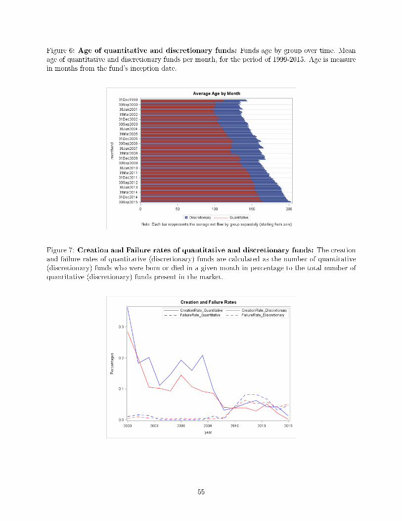
Figure 6: Age of quantitative and discretionary funds: Funds age by group over time. Meanage of quantitative and discretionary funds per month, for the period of 1999-2015. Age is measurein months from the fund's inception date.

Figure 7: Creation and Failure rates of quantitative and discretionary funds: The creationand failure rates of quantitative (discretionary) funds are calculated as the number of quantitative(discretionary) funds who were born or died in a given month in percentage to the total number ofquantitative (discretionary) funds present in the market.

55

Figure 8: Funds size by group: Distribution of quantitative and discretionary log-fund-size acrossthe entire sample.

Figure 9: Shortselling by quantitative and discretionary funds: Average percentage of grossTNA sold short by discretionary and quantitative funds over time. The table represents the shortpositions over time of a sample of 50 funds (36 discretionary and 24 quantitative) for which shortpositions are available in the CRSP Mutual Fund Holdings dataset. The % of gross TNA sold shortis computed as the relative value of the shares sold short relative to the gross TNA (value of long+ short positions). Eg: for a 130-30 strategy the weight displayed in the table would be 30% of thefund's TNA divided by 160% of the fund's TNA.

56

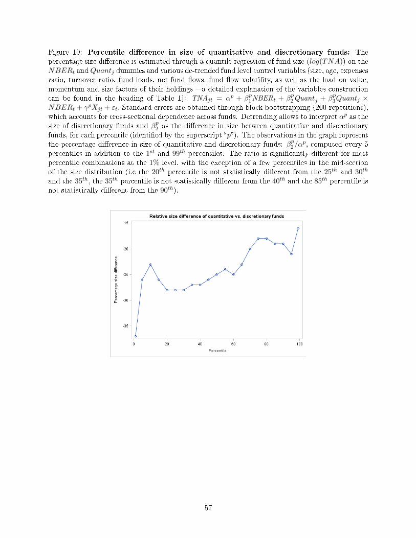
Figure 10: Percentile di�erence in size of quantitative and discretionary funds: Thepercentage size di�erence is estimated through a quantile regression of fund size (log(TNA)) on theNBERt andQuantj dummies and various de-trended fund level control variables (size, age, expensesratio, turnover ratio, fund loads, net fund �ows, fund �ow volatility, as well as the load on value,momentum and size factors of their holdings � a detailed explanation of the variables constructioncan be found in the heading of Table 1): TNAjt = αp + βp1NBERt + βp2Quant j + βp3Quantj ×NBERt + γpXjt + εt. Standard errors are obtained through block bootstrapping (200 repetitions),which accounts for cross-sectional dependence across funds. Detrending allows to interpret αp as thesize of discretionary funds and βp2 as the di�erence in size between quantitative and discretionaryfunds, for each percentile (identi�ed by the superscript �p�). The observations in the graph representthe percentage di�erence in size of quantitative and discretionary funds: βp2/α

p, computed every 5percentiles in addition to the 1st and 99th percentiles. The ratio is signi�cantly di�erent for mostpercentile combinations at the 1% level, with the exception of a few percentiles in the mid-sectionof the size distribution (i.e the 20th percentile is not statistically di�erent from the 25th and 30th

and the 35th, the 35th percentile is not statistically di�erent from the 40th and the 85th percentile isnot statistically di�erent from the 90th).

57

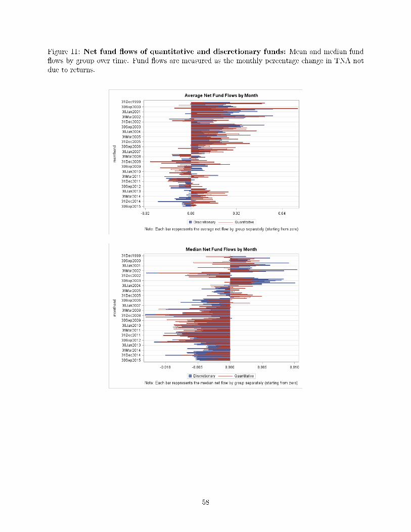
Figure 11: Net fund �ows of quantitative and discretionary funds: Mean and median fund�ows by group over time. Fund �ows are measured as the monthly percentage change in TNA notdue to returns.

58

Figure 12: Number of stocks held by quantitative and discretionary funds: Distribution ofthe number of stocks held by quantitative and discretionary funds over the entire period. Panel 1:displays the distribution in expansions. Panel 2: display the distributions in recessions.

Figure 13: Distribution of holdings dispersion and commonality of quantitative and dis-

cretionary funds: Panel 1 displays the distribution of the commonality measure by group. Com-monality is measured as the weighted average of the percentage of other quantitative (discretionary)funds who hold the same stocks. Weights are the normalized percentage of TNA that the fund in-vests in a certain stock (in excess of the market weight). Panel 2 displays the dispersion distributionby groups. Dispersion is measured as the cumulative squared weight weight allocated by funds toeach stock in excess of the average weight allocated by all funds of their type.

59

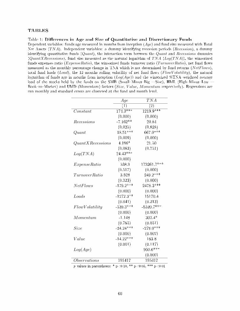
TABLES

Table 1: Di�erences in Age and Size of Quantitative and Discretionary FundsDependent variables: funds age measured in months from inception (Age) and fund size measured with TotalNet Assets (TNA). Independent variables: a dummy identifying recession periods (Recession), a dummyidentifying quantitative funds (Quant), the interaction term between the Quant and Recessions dummies(QuantXRecessions), fund size measured as the natural logarithm of TNA (Log(TNA)), the winsorizedfunds expenses ratio (ExpenseRatio), the winsorized funds turnover ratio (TurnoverRatio), net fund �owsmeasured as the monthly percentage change in TNA which is not determined by fund returns (NetF lows),total fund loads (Load), the 12�months rolling volatility of net fund �ows (FlowV olatility), the naturallogarithm of funds age in months from inception (Log(Age)) and the winsorized %TNA�weighted averageload of the stocks held by the funds on the SMB (Small�Minus�Big � Size), HML (High�Minus�Low �Book�to�Market) and UMD (Momentum) factors (Size, V alue, Momentum respectively). Regressions arerun monthly and standard errors are clustered at the fund and month level.

Age TNA(1) (2)

Constant 174.3*** 1219.9***(0.000) (0.000)

Recessions -7.162** 20.84(0.025) (0.828)

Quant -18.51*** -667.0***(0.009) (0.000)

QuantXRecessions 4.196* 21.50(0.083) (0.751)

Log(TNA) 24.43***(0.000)

ExpenseRatio -538.9 -173261.7***(0.517) (0.000)

TurnoverRatio -3.828 -249.2***(0.323) (0.000)

NetF lows -179.2*** 2478.3***(0.000) (0.000)

Loads -1272.3** 15170.4(0.041) (0.213)

FlowV olatility -539.3*** -5520.7***(0.000) (0.000)

Momentum -1.148 302.4*(0.765) (0.051)

Size -24.24*** -278.0***(0.000) (0.002)

V alue -14.22*** 163.8(0.001) (0.117)

Log(Age) 950.0***(0.000)

Observations 195417 195417

p-values in parentheses: * p<0.10, ** p<0.05, *** p<0.01

60

Table 2: Di�erences in the Holdings of Quantitative and Discretionary Funds

Dependent variables: the winsorized %TNA�weighted average load of the stocks held by each fundseach month on the SMB (Small�Minus�Big � Size), HML (High�Minus�Low � Book�to�Market)and UMD (Momentum) factors (Size, V alue, Momentum respectively), the winsorized turnoverratio in fund holdings (TurnoverRatio) and the amount of cash held (Cash). Independent variablesare the same as described in Table 1. Regressions are run monthly and standard errors are clusteredat the fund and month level.

Momentum Size V alue TurnoverRatio Cash(1) (2) (3) (4) (5)

Constant 0.00461 0.272*** -0.0594*** 0.757*** 3.174***(0.660) (0.000) (0.000) (0.000) (0.000)

Recessions -0.0107 -0.0625** 0.0753* 0.0976*** 0.504***(0.580) (0.023) (0.074) (0.000) (0.000)

Quant 0.00822* -0.0276 0.0770*** 0.147*** -0.730***(0.051) (0.210) (0.000) (0.000) (0.000)

QuantXRecessions -0.00977* 0.0314** -0.00492 0.00737 -0.668**(0.098) (0.016) (0.781) (0.793) (0.021)

Log(TNA) 0.00370*** 0.00745* 0.00268 -0.0175*** 0.145***(0.000) (0.068) (0.411) (0.007) (0.000)

ExpenseRatio 2.093*** 24.39*** 1.414 23.05*** 125.4***(0.000) (0.000) (0.399) (0.000) (0.000)

TurnoverRatio 0.0363*** 0.0356*** -0.0662*** -0.274**(0.000) (0.001) (0.000) (0.034)

NetF lows 0.0884*** 0.0436 0.289*** -0.355*** 4.225***(0.005) (0.335) (0.000) (0.000) (0.000)

Loads 0.936** 9.626*** -6.570 125.8(0.029) (0.001) (0.220) (0.171)

FlowV olatility 0.0102 0.517*** 0.456*** 1.695*** 3.325**(0.718) (0.000) (0.000) (0.000) (0.046)

Size -0.0141 0.0946*** 0.0714*** 0.541***(0.479) (0.000) (0.002) (0.000)

V alue -0.0194 0.0979*** -0.144*** 0.517***(0.401) (0.000) (0.000) (0.000)

Loads 0.480(0.894)

Momentum -0.0327 -0.0433 0.174*** -0.500***(0.491) (0.419) (0.000) (0.004)

Log(Age) -0.0295** -0.333***(0.048) (0.000)

Observations 195417 195417 195417 195417 173924

p-values in parentheses: * p<0.10, ** p<0.05, *** p<0.01

61

Table 3: Di�erences in NetFundFlows of Quantitative and Discretionary Funds

NetF lows F lowV olatility NetF lows2011(1) (2) (3)

Constant 0.00175*** 0.0337*** -0.00183**(0.001) (0.000) (0.012)

Recessions -0.000606 -0.000691(0.704) (0.313)

Quant -0.00104 0.00135 0.00449***(0.191) (0.252) (0.000)

QuantXRecessions -0.00520*** 0.00269(0.005) (0.101)

Log(Age) -0.00999*** -0.00891***(0.000) (0.000)

Log(TNA) 0.00321*** -0.00392***(0.000) (0.000)

ExpenseRatio 0.390*** -0.496***(0.000) (0.000)

TurnoverRatio -0.00252*** 0.00487***(0.000) (0.000)

Loads 0.177 -0.0407(0.271) (0.766)

FlowV olatility 0.329***(0.000)

Momentum 0.00324*** 0.000341(0.005) (0.677)

Size 0.0000805 0.00254***(0.901) (0.001)

V alue 0.00322*** 0.00172**(0.000) (0.014)

NetF lows 0.132***(0.000)

Observations 195417 195417 89772

p-values in parentheses: * p<0.10, ** p<0.05, *** p<0.01

62

Table 4: Di�erences in Fees Charged by Quantitative and Discretionary Funds

Dependent variables: funds expenses ratio (ExpenseRatio), management fees (ManagementFees),Actual_12b1 fee (Actual_12b1) and fund loads (Loads). Independent variables are the same asdescribed in Table 1. Regressions are run monthly and standard errors are clustered at the fund andmonth level.

ExpenseRatio ManagementFees Actual_12b1 Loads(1) (2) (3) (4)

Constant 0.0121*** 0.00694*** 0.00365*** 0.000233***(0.000) (0.000) (0.000) (0.000)

Recessions 0.0000578 0.000489*** 0.0000662 -0.0000446*(0.594) (0.000) (0.299) (0.067)

Quant -0.00135*** -0.000625*** 0.0000556 -0.00000609(0.000) (0.000) (0.706) (0.922)

QuantXRecessions -0.000152 -0.000152 -0.000155** 0.0000492(0.137) (0.303) (0.043) (0.325)

Log(Age) 0.0000247 0.000545*** -0.000171** -0.0000302(0.790) (0.000) (0.016) (0.205)

Log(TNA) -0.000673*** 0.000199*** -0.000000974 0.0000236(0.000) (0.000) (0.972) (0.147)

TurnoverRatio 0.000674*** 0.000427*** 0.000325*** -0.0000463(0.000) (0.000) (0.000) (0.309)

NetF lows 0.00159*** -0.00482*** -0.0000235 0.000173(0.000) (0.000) (0.930) (0.395)

Loads 0.186*** 0.128*** -0.0157(0.000) (0.000) (0.196)

FlowV olatility -0.00504*** -0.00660*** -0.00314*** -0.0000994(0.000) (0.000) (0.009) (0.769)

Momentum 0.000290*** 0.000222** 0.0000401 0.0000319(0.008) (0.048) (0.553) (0.523)

Size 0.00146*** 0.00145*** -0.0000852 0.00000510(0.000) (0.000) (0.353) (0.923)

V alue 0.0000904 0.0000329 0.0000488 0.000140*(0.387) (0.732) (0.529) (0.087)

ExpenseRatio 0.0447***(0.001)

Observations 195417 195389 126070 195417

p-values in parentheses: * p<0.10, ** p<0.05, *** p<0.01

63

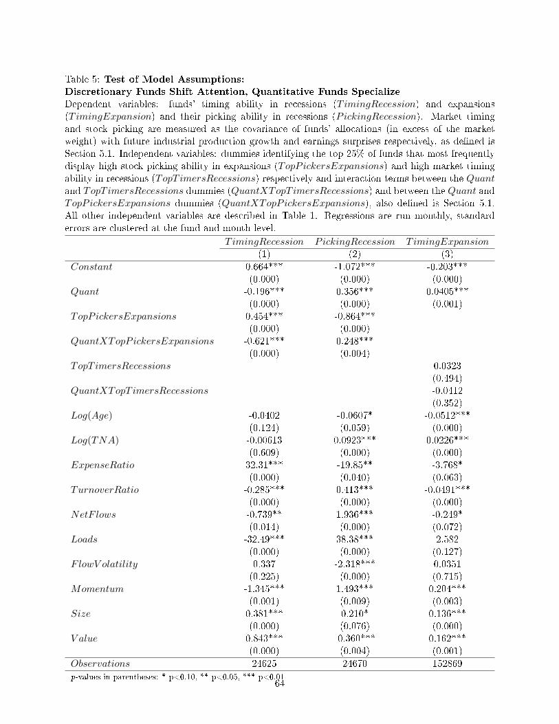
Table 5: Test of Model Assumptions:

Discretionary Funds Shift Attention, Quantitative Funds Specialize

Dependent variables: funds' timing ability in recessions (TimingRecession) and expansions(TimingExpansion) and their picking ability in recessions (PickingRecession). Market timingand stock picking are measured as the covariance of funds' allocations (in excess of the marketweight) with future industrial production growth and earnings surprises respectively, as de�ned isSection 5.1. Independent variables: dummies identifying the top 25% of funds that most frequentlydisplay high stock picking ability in expansions (TopP ickersExpansions) and high market timingability in recessions (TopT imersRecessions) respectively and interaction terms between the Quantand TopT imersRecessions dummies (QuantXTopT imersRecessions) and between the Quant andTopP ickersExpansions dummies (QuantXTopPickersExpansions), also de�ned is Section 5.1.All other independent variables are described in Table 1. Regressions are run monthly, standarderrors are clustered at the fund and month level.

TimingRecession PickingRecession T imingExpansion(1) (2) (3)

Constant 0.664*** -1.072*** -0.203***(0.000) (0.000) (0.000)

Quant -0.196*** 0.356*** 0.0405***(0.000) (0.000) (0.001)

TopP ickersExpansions 0.454*** -0.864***(0.000) (0.000)

QuantXTopPickersExpansions -0.621*** 0.248***(0.000) (0.004)

TopT imersRecessions 0.0323(0.494)

QuantXTopT imersRecessions -0.0412(0.352)

Log(Age) -0.0402 -0.0607* -0.0512***(0.124) (0.059) (0.000)

Log(TNA) -0.00613 0.0923*** 0.0226***(0.609) (0.000) (0.000)

ExpenseRatio 32.31*** -19.85** -3.768*(0.000) (0.040) (0.063)

TurnoverRatio -0.285*** 0.413*** -0.0491***(0.000) (0.000) (0.000)

NetF lows -0.739** 1.936*** -0.249*(0.014) (0.000) (0.072)

Loads -32.49*** 38.38*** 2.582(0.000) (0.000) (0.127)

FlowV olatility 0.337 -2.318*** 0.0351(0.225) (0.000) (0.715)

Momentum -1.345*** 1.493*** 0.204***(0.001) (0.009) (0.003)

Size 0.381*** 0.210* 0.136***(0.000) (0.076) (0.000)

V alue 0.843*** -0.360*** 0.162***(0.000) (0.004) (0.001)

Observations 24625 24670 152869

p-values in parentheses: * p<0.10, ** p<0.05, *** p<0.0164

Table 6: Number of Stocks Held by Quantitative and Discretionary Funds

Dependent variable: number of stocks held (Number_holdings). Independent variables:dummies for quantitative funds (Quant) and recessions (Recessions) and their interaction(QuantXRecessions); amount of cash held (Cash) and the fund log�size measured as the natu-ral logarithm of total net assets (Log(TNA)).

Number of Stocks Held(1) (2)

Constant 117.6*** 160.2***(0.000) (0.000)

Quant 108.4*** 124.8***(0.000) (0.000)

Recessions -4.985 2.067(0.128) (0.648)

QuantXRecessions 21.27*** 12.85(0.005) (0.128)

Cash -0.722(0.274)

Log(TNA) 26.47***(0.000)

Observations 229742 173926

p-values in parentheses: * p<0.10, ** p<0.05, *** p<0.01

65

Table7:PortfolioRiskofQuantitativeandDiscretionary

Funds

Dependentvariables:

12�m

onthsand36�m

onthsrollingvolatility

offundreturns(Vol_

12m

andVol_

36m

respectively),

CAPM

id-

iosyncraticvolatility

(IVCapm_

12m

andIVCapm_

36m

respectively),Fam

a�French

3�factorsidiosyncraticvolatility

(IVFF_

12m

and

IVFF_

36m

respectively)andCAR4�factor

idiosyncraticvolatility

(IVCar_

12m

andIVCar_

36m

respectively).Idiosyncraticvolatil-

ityiscalculatedas

thevolatility

oftheresidual

ofaregression

offundreturnson

themarketfactor

(CAPM)thesize

andvaluefactors

(3�factors)andthemom

entum

factor

(4�factors).

Independentvariablesarethesameas

described

inTable

1.Regressionsarerun

monthly,standarderrors

areclustered

atthefundandmonth

level.

Vol_

12m

Vol_

36m

IVolCapm_

12m

IVolCapm_

36m

IVolFF_

12m

IVolFF_

36m

IVolCar_

12m

IVolCar_

36m

(1)

(2)

(3)

(4)

(5)

(6)

(7)

(8)

Constant

4.319***

4.915***

1.578***

1.763***

1.192***

1.413***

1.150***

1.365***

(0.000)

(0.000)

(0.000)

(0.000)

(0.000)

(0.000)

(0.000)

(0.000)

Recessions

1.780***

0.706***

0.740***

0.697***

(0.000)

(0.000)

(0.000)

(0.000)

Quant

-0.0825**

-0.108***

-0.152***

-0.147***

-0.183***

-0.186***

-0.179***

-0.186***

(0.012)

(0.008)

(0.000)

(0.000)

(0.000)

(0.000)

(0.000)

(0.000)

QuantXRecess

-0.146***

-0.0616*

-0.0385

-0.0351

(0.002)

(0.056)

(0.186)

(0.205)

Log

(Age)

-0.0274

0.00279

-0.0735***

-0.0647***

-0.0569***

-0.0430***

-0.0482***

-0.0315**

(0.405)

(0.936)

(0.000)

(0.000)

(0.000)

(0.003)

(0.000)

(0.019)

Log

(TNA

)-0.0170

-0.00316

0.0322***

0.0319***

0.0236***

0.0229***

0.0202***

0.0196***

(0.258)

(0.831)

(0.000)

(0.000)

(0.000)

(0.000)

(0.000)

(0.001)

ExpenseRatio

16.03**

30.46***

44.43***

53.94***

44.82***

51.33***

42.80***

48.94***

(0.023)

(0.000)

(0.000)

(0.000)

(0.000)

(0.000)

(0.000)

(0.000)

TurnoverRatio

0.336***

0.414***

0.212***

0.261***

0.195***

0.244***

0.172***

0.213***

(0.000)

(0.000)

(0.000)

(0.000)

(0.000)

(0.000)

(0.000)

(0.000)

NetFlows

-0.886***

-0.737***

-0.109

-0.0853

-0.00832

-0.0622

-0.00967

-0.0714

(0.000)

(0.001)

(0.323)

(0.451)

(0.921)

(0.498)

(0.901)

(0.396)

Loads

7.541

4.323

6.141

6.092

1.612

2.809

0.287

1.927

(0.216)

(0.579)

(0.178)

(0.210)

(0.672)

(0.524)

(0.937)

(0.647)

FlowVolatility

1.472***

0.494

1.927***

1.025***

1.443***

0.865***

1.417***

0.928***

(0.000)

(0.250)

(0.000)

(0.000)

(0.000)

(0.000)

(0.000)

(0.000)

Mom

entum

-0.421***

-0.690***

0.0445

0.0173

-0.110**

-0.0778*

-0.144***

-0.0926**

(0.010)

(0.000)

(0.461)

(0.746)

(0.014)

(0.065)

(0.000)

(0.025)

Size

0.854***

0.688***

0.791***

0.724***

0.239***

0.272***

0.266***

0.283***

(0.000)

(0.000)

(0.000)

(0.000)

(0.000)

(0.000)

(0.000)

(0.000)

Value

-0.436***

-0.213***

0.00469

-0.00253

-0.105***

-0.0652**

-0.107***

-0.0745***

(0.000)

(0.001)

(0.914)

(0.949)

(0.001)

(0.017)

(0.001)

(0.004)

Observations

186427

186427

187822

178979

187822

178979

187822

178979

p-values

inparentheses:*p<0.10,**p<0.05,***p<0.01

66

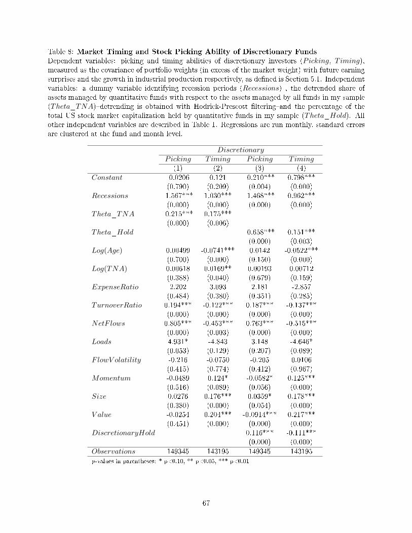
Table 8: Market Timing and Stock Picking Ability of Discretionary Funds

Dependent variables: picking and timing abilities of discretionary investors (Picking, Timing),measured as the covariance of portfolio weights (in excess of the market weight) with future earningsurprises and the growth in industrial production respectively, as de�ned is Section 5.1. Independentvariables: a dummy variable identifying recession periods (Recessions) , the detrended share ofassets managed by quantitative funds with respect to the assets managed by all funds in my sample(Theta_TNA)�detrending is obtained with Hodrick-Prescott �ltering�and the percentage of thetotal US stock market capitalization held by quantitative funds in my sample (Theta_Hold). Allother independent variables are described in Table 1. Regressions are run monthly, standard errorsare clustered at the fund and month level.

DiscretionaryP icking T iming P icking T iming

(1) (2) (3) (4)

Constant -0.0206 0.121 -0.210*** 0.798***(0.790) (0.209) (0.004) (0.000)

Recessions -1.567*** 1.030*** -1.468*** 0.962***(0.000) (0.000) (0.000) (0.000)

Theta_TNA -0.215*** 0.175***(0.000) (0.006)

Theta_Hold -0.658*** 0.151***(0.000) (0.003)

Log(Age) 0.00499 -0.0741*** 0.0142 -0.0522***(0.700) (0.000) (0.150) (0.000)

Log(TNA) 0.00618 0.0169** 0.00193 0.00712(0.388) (0.040) (0.679) (0.159)

ExpenseRatio 2.202 3.093 2.181 -2.857(0.484) (0.380) (0.351) (0.285)

TurnoverRatio 0.194*** -0.122*** 0.187*** -0.137***(0.000) (0.000) (0.000) (0.000)

NetF lows 0.805*** -0.453*** 0.763*** -0.515***(0.000) (0.003) (0.000) (0.000)

Loads 4.931* -4.843 3.148 -4.646*(0.053) (0.129) (0.207) (0.089)

FlowV olatility -0.216 -0.0750 -0.205 0.0106(0.415) (0.774) (0.412) (0.967)

Momentum -0.0489 0.124* -0.0582* 0.125***(0.516) (0.089) (0.056) (0.000)

Size 0.0276 0.176*** 0.0359* 0.178***(0.380) (0.000) (0.054) (0.000)

V alue -0.0254 0.204*** -0.0914*** 0.217***(0.451) (0.000) (0.000) (0.000)

DiscretionaryHold 0.116*** -0.111***(0.000) (0.000)

Observations 149345 143195 149345 143195

p-values in parentheses: * p<0.10, ** p<0.05, *** p<0.01

67

Table 9: Size of Stocks Held by Discretionary Funds

Independent variable: average market capitalization of stocks stocks held measured with simpleaverage (MarketV alue), average weighted by %TNA (MarketV alue_w) and weighted by %TNAin excess of the market weight (MarketV alue_wd), as de�ned is Section 5.1. Dependent variables:dummy variables identifying discretionary funds (Discretionary), and recessions (Recessions) andan interaction term between the two dummies (DiscretXRecessions).

MarketV alue MarketV alue_w MarketV alue_wd(1) (2) (3)

Constant 24449575.8*** 42867071.0*** 33420522.1***(0.000) (0.000) (0.000)

Discretionary 599454.1 -7149830.3** -5664176.9*(0.697) (0.015) (0.080)

Recessions -1055761.5 -2079402.3 -2243909.5(0.306) (0.280) (0.439)

DiscretXRecessions -149161.7 666792.0 589729.2(0.834) (0.712) (0.836)

Observations 133957 133957 133957

p-values in parentheses: * p<0.10, ** p<0.05, *** p<0.01

Table 10: Age of Stocks Held by Discretionary Funds

Dependent variable: average age of stocks held (in months from inception), simple average(Stocks_Age), %TNA�weighted average (Stocks_Age_w) and %TNA�di�erence weighted aver-age (Stocks_Age_wd), as de�ned is Section 5.1. Dependent variables as in table 9.

Stocks_Age Stocks_Age_w Stocks_Age_wd(1) (2) (3) (4) (5)

Constant 317.0*** 340.3*** 335.8*** 335.0*** 327.6***(0.000) (0.000) (0.000) (0.000) (0.000)

Discretionary -27.84*** -35.51*** -34.77*** -36.81*** -35.58***(0.000) (0.000) (0.000) (0.000) (0.000)

Recessions -5.815 5.820 6.036 3.051 3.410(0.239) (0.370) (0.351) (0.606) (0.569)

DiscretXRecessions 0.510 -4.968 -5.038 -2.301 -2.416(0.809) (0.140) (0.135) (0.387) (0.358)

MarketV alue_w 0.000000104 0.000000172(0.570) (0.274)

Observations 133957 133957 133957 133957 133957

p-values in parentheses: * p<0.10, ** p<0.05, *** p<0.01

68

Table 11: Media Mentions of Stocks Held by Discretionary Funds

Dependent variable: average number of times stock held are mentioned in Dow Jones newsper month, simple average (Media), %TNA�weighted average (Media_w) and %TNA�di�erenceweighted average (Media_wd), as de�ned is Section 5.1. Dependent variables as in table 9.

Media Media_w Media_wd(1) (2) (3) (4) (5)

Constant 245.5*** 352.3*** -67.51*** 293.8*** 275.0***(0.000) (0.000) (0.000) (0.000) (0.000)

Discretionary 8.622 -56.64** 13.37 -33.77** -30.63**(0.527) (0.014) (0.175) (0.035) (0.043)

Recessions 19.57* 8.349 28.71* 21.65 22.56(0.087) (0.692) (0.069) (0.134) (0.113)

DiscretXRecessions 17.17*** 20.82 14.29* 3.884 3.591(0.001) (0.173) (0.076) (0.542) (0.570)

MarketV alue_w 0.00000979*** 0.000000439(0.000) (0.280)

Observations 133957 133957 133957 133957 133957

p-values in parentheses: * p<0.10, ** p<0.05, *** p<0.01

Table 12: Analysts Coverage of Stocks Held by Discretionary Funds

Dependent variable: average number of forecasts made by analysts on stocks held, simple aver-age (Analysts), %TNA�weighted average (Analysts_w) and %TNA�di�erence weighted average(Analysts_wd), as de�ned is Section 5.1. Dependent variables as in table 9.

Analysts Analysts_w Analysts_wd(1) (2) (3) (4) (5)

Constant 374.7*** 192.7*** 410.1*** 394.9*** 385.6***(0.000) (0.000) (0.000) (0.000) (0.000)

Discretionary 5.115 20.57** -15.69 -6.431 -4.880(0.619) (0.031) (0.249) (0.556) (0.647)

Recessions -121.9*** -131.2*** -141.7*** -130.3*** -129.8***(0.000) (0.000) (0.000) (0.000) (0.000)

DiscretXRecessions -0.641 8.862 12.24 2.401 2.256(0.924) (0.259) (0.212) (0.715) (0.732)

MarketV alue_w 0.00000507*** 0.000000217(0.000) (0.266)

Observations 133957 133957 133957 133957 133957

p-values in parentheses: * p<0.10, ** p<0.05, *** p<0.01

69

Table 13: Performance of Funds Holding Stocks with Smaller Information Gap

Dependent variables: 12�months rolling CAPM, Fama�French 3�factors and Carhart 4�factors al-phas. Independent variables: dummy variables that identify recession periods (Recessions) anddiscretionary funds (Discretionary) and an interaction between the two (DiscretXRecessions);active information gap measured in terms of the number of analysts following the stocks held(Analysts_wd), the age of stocks held (Stocks_Age_wd) and the number of times stocks heldare mentioned monthly in Dow Jones news (Media_wd). Are also included interaction terms be-tween all active information gap measures and the discretionary dummy (DisctretXAnalysts_wd,DisctretXStocks_Age_wd, DisctretXMedia_wd). The active information gap is constructed asthe weighted average of the age, number of media mentions and number of analysts forecasts forthe stocks held each month by each fund. The weights used are the normalized weight di�erencesof the % of TNA allocated by each fund to stocks minus their weight in the market, as de�ned isSection 5.1. Control variables are omitted for brevity; the controls used are the same in Table 1.Regressions are run monthly, standard errors are clustered at the fund and month level.

12 Months Rolling AlphasCAPM 3− Factor 4− Factor(1) (2) (3)

Recessions 0.126*** 0.0814*** 0.0164(0.000) (0.000) (0.132)

Discretionary 0.0771*** 0.156*** 0.119***(0.000) (0.000) (0.000)

DiscretXRecessions 0.0925*** 0.0167 0.0213*(0.000) (0.232) (0.099)

Analysts_wd -0.000328*** -0.000188*** -0.000261***(0.000) (0.000) (0.000)

DisctretXAnalysts_wd -0.000117*** -0.000201*** -0.000163***(0.000) (0.000) (0.000)

Stocks_Age_wd -0.000349*** 0.000297*** -0.0000341(0.000) (0.000) (0.402)

DisctretXStocks_Age_wd 0.0000329 -0.000118** -0.0000619(0.522) (0.017) (0.177)

Media_wd -0.000313*** -0.000247*** -0.000228***(0.000) (0.000) (0.000)

DisctretXMedia_wd -0.000120*** -0.0000458*** -0.0000567***(0.000) (0.010) (0.000)

Constant 0.895*** 0.184*** 0.360***(0.000) (0.000) (0.000)

Observations 127757 127757 127757

p-values in parentheses * p<0.10, ** p<0.05, *** p<0.01

70

Table 14: Di�erences in Holdings Dispersion and Commonality among Discretionary

and Quantitative funds

Dependent variables: dispersion (Dispersion) and commonality (Commonality) in holdings.Whereby commonality is de�ned as the allocation-weighted average of the percentage of funds ofthe same group which hold each stock over time and Dispersion is de�ned as the cumulative squareddi�erence in the weight allocated by each funds and the average weight allocated by funds of thesame type to each stock, as described is Section 5.1. Independent variables: a dummy indicatingdiscretionary funds (Discretionary), a dummy indicating recession periods (Recessions)and an in-teraction term between the two dummies (DiscretXRecessions). All other variables are describedin Table 1. Regressions are run monthly, standard errors are clustered at the fund and month level.

Dispersion Commonality

(1) (2)

intercept 0.00839∗∗∗ 14.79∗∗∗

(0.000) (0.000)

Discretionary 0.00257∗∗∗ -5.782∗∗∗

(0.000) (0.000)

Recessions 0.00173∗∗∗ 1.140∗∗∗

(0.005) (0.000)

DiscretXRecessions 0.000135 -1.353∗∗∗

(0.783) (0.000)

Controls Yes YesClustering Yes Yes

p-values in parentheses * p<0.10, ** p<0.05, *** p<0.01

71

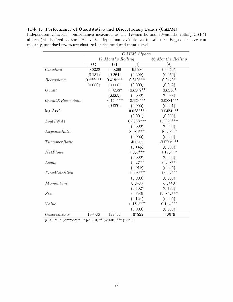
Table 15: Performance of Quantitative and Discretionary Funds (CAPM)

Independent variables: performance measured as the 12�months and 36�months rolling CAPMalphas (windsorized at the 1% level). Dependent variables as in table 9. Regressions are runmonthly, standard errors are clustered at the fund and month level.

CAPM Alphas12 Months Rolling 36 Months Rolling

(1) (2) (3) (4)

Constant -0.0328 -0.0266 -0.0286 0.0360*(0.131) (0.264) (0.209) (0.069)

Recessions 0.282*** 0.319*** 0.310*** 0.0479*(0.000) (0.000) (0.000) (0.059)

Quant -0.0268* -0.0269** -0.0214*(0.069) (0.050) (0.098)

QuantXRecessions -0.164*** -0.153*** -0.0884***(0.000) (0.000) (0.001)

log(Age) -0.0286*** -0.0454***(0.001) (0.000)

Log(TNA) 0.0288*** 0.0393***(0.000) (0.000)

ExpenseRatio 8.080*** 10.29***(0.000) (0.000)

TurnoverRatio -0.0200 -0.0296***(0.145) (0.003)

NetF lows 1.952*** 1.125***(0.000) (0.000)

Loads 7.027** 6.208**(0.019) (0.029)

FlowV olatility 1.098*** 1.003***(0.000) (0.000)

Momentum 0.0488 0.0440(0.302) (0.188)

Size 0.0586 0.0852***(0.124) (0.000)

V alue 0.163*** 0.134***(0.000) (0.000)

Observations 199566 199566 187822 178979

p-values in parentheses: * p<0.10, ** p<0.05, *** p<0.01

72

Table 16: Performance of Quantitative and Discretionary Funds (3-Factor Model)

Independent variables: performance measured as the 12�months and 36�months rolling Fama�French3�factor alphas (excess return on the market, SMB, HML � windsorized at the 1% level). Dependentvariables as in table 9. Regressions are run monthly, standard errors are clustered at the fund andmonth level.

3− Factor Alphas12 Months Rolling 36 Months Rolling

(1) (2) (3) (4)

Constant -0.0775*** -0.0710*** -0.0672*** -0.0329***(0.000) (0.000) (0.000) (0.004)

recession 0.0641 0.0864** 0.0849** 0.107***(0.112) (0.039) (0.035) (0.000)

Quant -0.0284** -0.0208* -0.0303***(0.031) (0.091) (0.004)

QuantXRecessions -0.0979*** -0.0886*** -0.0862***(0.001) (0.002) (0.000)

Log(Age) -0.0130** -0.0198***(0.047) (0.001)

Log(TNA) 0.0183*** 0.0276***(0.000) (0.000)

ExpenseRatio 1.026 1.626(0.457) (0.169)

TurnoverRatio -0.0816*** -0.0660***(0.000) (0.000)

NetF lows 1.417*** 0.872***(0.000) (0.000)

Loads 0.954 1.402(0.714) (0.396)

FlowV olatility 0.826*** 0.859***(0.000) (0.000)

Momentum 0.0529 0.0608***(0.114) (0.002)

Size 0.0370* 0.0289***(0.091) (0.002)

V alue 0.0649* 0.0111(0.065) (0.446)

Observations 199566 199566 187822 178979

p-values in parentheses: * p<0.10, ** p<0.05, *** p<0.01

73

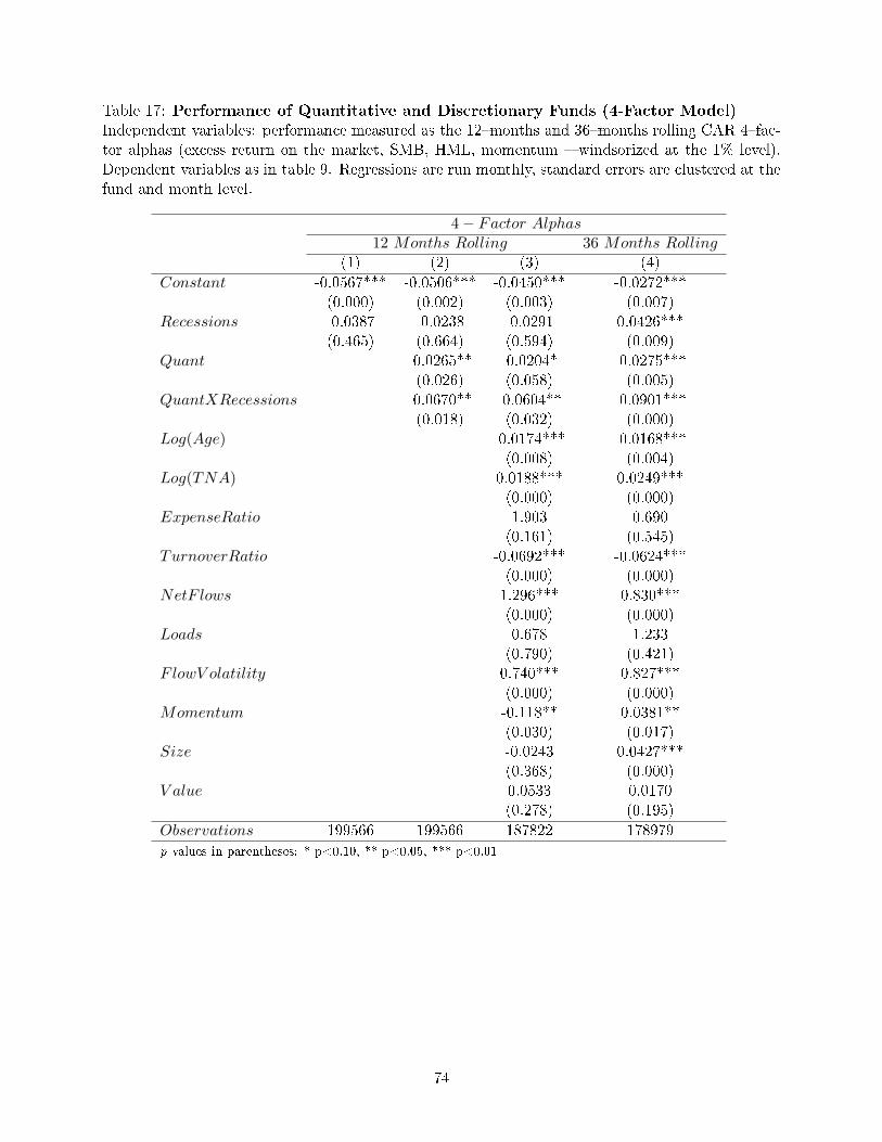
Table 17: Performance of Quantitative and Discretionary Funds (4-Factor Model)

Independent variables: performance measured as the 12�months and 36�months rolling CAR 4�fac-tor alphas (excess return on the market, SMB, HML, momentum � windsorized at the 1% level).Dependent variables as in table 9. Regressions are run monthly, standard errors are clustered at thefund and month level.

4− Factor Alphas12 Months Rolling 36 Months Rolling

(1) (2) (3) (4)

Constant -0.0567*** -0.0506*** -0.0450*** -0.0272***(0.000) (0.002) (0.003) (0.007)

Recessions -0.0387 -0.0238 -0.0291 0.0426***(0.465) (0.664) (0.594) (0.009)

Quant -0.0265** -0.0204* -0.0275***(0.026) (0.058) (0.005)

QuantXRecessions -0.0670** -0.0604** -0.0901***(0.018) (0.032) (0.000)

Log(Age) -0.0174*** -0.0168***(0.008) (0.004)

Log(TNA) 0.0188*** 0.0249***(0.000) (0.000)

ExpenseRatio 1.903 0.690(0.161) (0.545)

TurnoverRatio -0.0692*** -0.0624***(0.000) (0.000)

NetF lows 1.296*** 0.830***(0.000) (0.000)

Loads 0.678 1.233(0.790) (0.421)

FlowV olatility 0.740*** 0.827***(0.000) (0.000)

Momentum -0.118** 0.0381**(0.030) (0.017)

Size -0.0243 0.0427***(0.368) (0.000)

V alue 0.0533 0.0170(0.278) (0.195)

Observations 199566 199566 187822 178979

p-values in parentheses: * p<0.10, ** p<0.05, *** p<0.01

74

Table 18: Overcrowding and Performance of Quantitative Funds

Independent variable: performance as 12�months rolling CAPM alphas (Alphas) and Sharpe Ratio(SR). Dependent variables: E1, E2 and Recessions are dummies identifying the �rst two expansionsand all recessions in my sample respectively; holdings commonality (Commonality) de�ned as theallocation-weighted average of the percentage of other quantitative funds which hold each stock overtime (as described is Section 5.1); and a dummy which assumes a value of 1 when the commonalitymeasure is above the median (DCommonality).

12 Months RollingAlphas SR Alphas

CAPM 3− Factor 4− Factor CAPM CAPM

(1) (2) (3) (4) (5) (6)

Constant -0.106*** -0.105*** -0.0879*** 0.251** 0.00906 -0.0530(0.000) (0.000) (0.000) (0.019) (0.891) (0.194)

E1 0.798*** 0.404*** 0.460*** -0.581* 0.758*** 0.768***(0.000) (0.000) (0.000) (0.087) (0.000) (0.000)

E2 0.121*** -0.00883 0.00869 -0.0613 0.106*** 0.107***(0.001) (0.696) (0.709) (0.686) (0.006) (0.006)

Recessions 0.207*** -0.00384 -0.0809 -0.532** 0.215*** 0.209***(0.000) (0.932) (0.133) (0.036) (0.000) (0.000)

Commonality -0.773**(0.028)

DCommonality -0.0887**(0.040)

Observations 53147 53147 53147 52546 43348 43348

p-values in parentheses: * p<0.10, ** p<0.05, *** p<0.01

75