malware classification based on hidden markov model and
TRANSCRIPT
San Jose State University San Jose State University
SJSU ScholarWorks SJSU ScholarWorks
Master's Projects Master's Theses and Graduate Research
Spring 5-20-2020
Malware Classification Based on Hidden Markov Model and Malware Classification Based on Hidden Markov Model and
Word2Vec Features Word2Vec Features
Aparna Sunil Kale San Jose State University
Follow this and additional works at: https://scholarworks.sjsu.edu/etd_projects
Part of the Artificial Intelligence and Robotics Commons, and the Information Security Commons
Recommended Citation Recommended Citation Kale, Aparna Sunil, "Malware Classification Based on Hidden Markov Model and Word2Vec Features" (2020). Master's Projects. 921. DOI: https://doi.org/10.31979/etd.edkg-dtq8 https://scholarworks.sjsu.edu/etd_projects/921
This Master's Project is brought to you for free and open access by the Master's Theses and Graduate Research at SJSU ScholarWorks. It has been accepted for inclusion in Master's Projects by an authorized administrator of SJSU ScholarWorks. For more information, please contact [email protected].

Malware Classification Based on Hidden Markov Model and Word2Vec Features
A Project
Presented to
The Faculty of the Department of Computer Science
San José State University
In Partial Fulfillment
of the Requirements for the Degree
Master of Science
by
Aparna Sunil Kale
May 2020

© 2020
Aparna Sunil Kale
ALL RIGHTS RESERVED

The Designated Project Committee Approves the Project Titled
Malware Classification Based on Hidden Markov Model and Word2Vec Features
by
Aparna Sunil Kale
APPROVED FOR THE DEPARTMENT OF COMPUTER SCIENCE
SAN JOSÉ STATE UNIVERSITY
May 2020
Dr. Mark Stamp Department of Computer Science
Dr. Thomas Austin Department of Computer Science
Fabio Di Troia Department of Computer Science

ABSTRACT
Malware Classification Based on Hidden Markov Model and Word2Vec Features
by Aparna Sunil Kale
Malware classification is an important and challenging problem in information
security. Modern malware classification techniques rely on machine learning models
that can be trained on a wide variety of features, including opcode sequences, API
calls, and byte 𝑛-grams, among many others. In this research, we implement hybrid
machine learning techniques, where we train hidden Markov models (HMM) and
compute Word2Vec encodings based on opcode sequences. The resulting trained
HMMs and Word2Vec embedding vectors are then used as features for classification
algorithms. Specifically, we consider support vector machine (SVM), 𝑘-nearest neighbor
(𝑘-NN), random forest (RF), and deep neural network (DNN) classifiers. We conduct
substantial experiments over a variety of malware families. Our results surpass those
of comparable classification experiments.

ACKNOWLEDGMENTS
I want to express my gratitude towards Dr. Mark Stamp for his continuous support
and motivation throughout my thesis work. I am fortunate to have Dr. Stamp as my
advisor, as he inspired me to push the limits during the research and experiments.
I am grateful to my committee members Dr. Thomas Austin and Fabio Di Troia,
for their suggestions, feedback, and dataset related help.
I want to thank my parents for always believing in me and guiding me in my
career milestones.
v

TABLE OF CONTENTS
CHAPTER
1 Introduction . . . . . . . . . . . . . . . . . . . . . . . . . . . . . . . . 1
2 Background . . . . . . . . . . . . . . . . . . . . . . . . . . . . . . . . 3
2.1 Signature-based malware detection . . . . . . . . . . . . . . . . . 3
2.2 Behavioral-based malware detection . . . . . . . . . . . . . . . . . 4
2.3 Machine learning models for malware classification . . . . . . . . . 4
2.3.1 Hidden Markov model . . . . . . . . . . . . . . . . . . . . 4
2.3.2 Word2Vec embeddings . . . . . . . . . . . . . . . . . . . . 5
2.3.3 Random forest . . . . . . . . . . . . . . . . . . . . . . . . . 5
2.3.4 𝑘-nearest neighbors (𝑘NN) . . . . . . . . . . . . . . . . . . 6
2.3.5 Support vector machine . . . . . . . . . . . . . . . . . . . 7
2.3.6 Deep neural network . . . . . . . . . . . . . . . . . . . . . 7
2.4 Previous work . . . . . . . . . . . . . . . . . . . . . . . . . . . . . 8
3 Implementation . . . . . . . . . . . . . . . . . . . . . . . . . . . . . . 10
3.1 Dataset . . . . . . . . . . . . . . . . . . . . . . . . . . . . . . . . 10
3.2 Hybrid classification techniques . . . . . . . . . . . . . . . . . . . 12
3.2.1 Hybrid machine learning based on HMMs . . . . . . . . . . 12
3.2.2 Hybrid machine learning based on Word2Vec embeddings . 14
4 Results and Analysis . . . . . . . . . . . . . . . . . . . . . . . . . . 15
4.1 Binary classification to determine the number of opcodes . . . . . 15
4.1.1 Training Word2Vec . . . . . . . . . . . . . . . . . . . . . . 15
vi

vii
4.1.2 Word2Vec-SVM for binary classification . . . . . . . . . . . 16
4.2 Multiclass malware classification . . . . . . . . . . . . . . . . . . . 17
4.2.1 Training HMMs . . . . . . . . . . . . . . . . . . . . . . . . 17
4.2.2 HMM-SVM . . . . . . . . . . . . . . . . . . . . . . . . . . 18
4.2.3 HMM-𝑘NN . . . . . . . . . . . . . . . . . . . . . . . . . . 20
4.2.4 HMM-RF . . . . . . . . . . . . . . . . . . . . . . . . . . . 23
4.2.5 HMM-DNN . . . . . . . . . . . . . . . . . . . . . . . . . . 26
4.2.6 Word2Vec-SVM . . . . . . . . . . . . . . . . . . . . . . . . 29
4.2.7 Word2Vec-RF . . . . . . . . . . . . . . . . . . . . . . . . . 33
4.2.8 Word2Vec-𝑘NN . . . . . . . . . . . . . . . . . . . . . . . . 34
4.2.9 Word2Vec-DNN . . . . . . . . . . . . . . . . . . . . . . . . 36
4.3 Robustness analysis of hybrid machine learning techniques . . . . 40
4.3.1 Robustness of HMM-based techniques . . . . . . . . . . . . 41
4.3.2 Robustness of Word2Vec-based techniques . . . . . . . . . 42
5 Conclusion and Future Work . . . . . . . . . . . . . . . . . . . . . 46
LIST OF REFERENCES . . . . . . . . . . . . . . . . . . . . . . . . . . . 49
APPENDIX
Additional results . . . . . . . . . . . . . . . . . . . . . . . . . . . . . . . . 53
A.1 HMM-SVM: Binary classification of Winwebsec and Zbot malwarefamilies . . . . . . . . . . . . . . . . . . . . . . . . . . . . . . 53
A.2 HMM-𝑘NN: Binary classification of Winwebsec and Zbot malwarefamilies . . . . . . . . . . . . . . . . . . . . . . . . . . . . . . 54
A.3 Word2Vec-RF: Multiclass classification . . . . . . . . . . . . . . . 55
A.4 Word2Vec-𝑘NN: Multiclass classification . . . . . . . . . . . . . . 55

LIST OF TABLES
1 HMM-SVM accuracies . . . . . . . . . . . . . . . . . . . . . . . . 20
2 Randomized search parameters for HMM-RF . . . . . . . . . . . 24
3 Word2Vec-SVM grid search accuracies, vector size = 2 andwindow size = 30 . . . . . . . . . . . . . . . . . . . . . . . . . . . 32
4 Randomized search parameters for Word2Vec-RF . . . . . . . . . 34
A.5 HMM-SVM accuracies . . . . . . . . . . . . . . . . . . . . . . . . 55
viii

LIST OF FIGURES
1 Number of samples per family . . . . . . . . . . . . . . . . . . . . 11
2 Percentage of 31 frequent opcodes from 50 malware families withhighest number of samples . . . . . . . . . . . . . . . . . . . . . 12
3 Word2Vec-SVM: Binary classification of Winwebsec and Fakerean 16
4 HMM-SVM, Accuracy vs 𝐶 . . . . . . . . . . . . . . . . . . . . . 19
5 Confusion matrix for HMM-SVM with linear kernel . . . . . . . . 19
6 Confusion matrix for HMM-𝑘NN with 𝑘 = 70 . . . . . . . . . . . 21
7 HMM-𝑘NN, cross-validation: Average accuracy for varying𝑘-neighbors, using 𝐵 vectors . . . . . . . . . . . . . . . . . . . . . 22
8 Confusion matrix for HMM-RF . . . . . . . . . . . . . . . . . . . 24
9 Confusion matrix for HMM-RF using grid parameters . . . . . . . 25
10 HMM-RF cross-validation, average accuracy across 10 folds . . . 25
11 Model accuracy for HMM-DNN — overfitting . . . . . . . . . . . 28
12 Model loss for HMM-DNN — overfitting . . . . . . . . . . . . . . 28
13 HMM-DNN model architecture . . . . . . . . . . . . . . . . . . . 29
14 Model accuracy and loss for HMM-DNN . . . . . . . . . . . . . . 30
15 Word2Vec-SVM, linear kernel: Accuracy vs different vector andwindow sizes . . . . . . . . . . . . . . . . . . . . . . . . . . . . . 31
16 Word2Vec-SVM, RBF kernel: Accuracy vs different vector andwindow sizes . . . . . . . . . . . . . . . . . . . . . . . . . . . . . 32
17 Word2Vec-RF classification vector size = 100 and window size = 30 34
18 Word2Vec-RF cross-validation: Average accuracy across 10 folds,vector size = 100 and window size = 30 . . . . . . . . . . . . . . . 35
ix

x
19 Word2Vec-𝑘NN cross-validation: Average accuracy for varying𝑘-neighbors, vector size = 100 and window size = 1 . . . . . . . . 36
20 Confusion matrix for Word2Vec-𝑘NN for 𝑘-neighbors = 7,vector size = 100 and window size = 1 . . . . . . . . . . . . . . . 37
21 Model accuracy and loss for Word2Vec-DNN, vector size = 31,window size = 1 and epochs = 100 . . . . . . . . . . . . . . . . . 38
22 Model accuracy and loss for Word2Vec-DNN, vector size = 31,window size = 1 and epochs = 50 . . . . . . . . . . . . . . . . . . 38
23 Confusion matrix: vector size = 31, window size = 1 andepochs = 15 . . . . . . . . . . . . . . . . . . . . . . . . . . . . . . 39
24 Accuracies across all Word2Vec-DNN experiments . . . . . . . . . 40
25 Robustness experiment for HMM-based hybrid machine learningtechniques . . . . . . . . . . . . . . . . . . . . . . . . . . . . . . . 41
26 Robustness experiment for Word2Vec-SVM . . . . . . . . . . . . 42
27 Robustness experiment for Word2Vec-𝑘NN . . . . . . . . . . . . . 43
28 Robustness experiment for Word2Vec-RF . . . . . . . . . . . . . . 44
29 Robustness experiment for Word2Vec-DNN . . . . . . . . . . . . 44
30 Best accuracies for HMM-based hybrid machine learning . . . . . 47
A.31 PR curve for HMM-SVM . . . . . . . . . . . . . . . . . . . . . . 53
A.32 ROC curve for HMM-SVM . . . . . . . . . . . . . . . . . . . . . 54
A.33 Mean score of cross-validation vs 𝑘-neighbors . . . . . . . . . . . 54
A.34 Word2Vec-𝑘NN classification vector size = 2 and window size = 1 56
A.35 Word2Vec-𝑘NN classification vector size = 2 and window size = 5 56
A.36 Word2Vec-𝑘NN classification vector size = 2 and window size = 10 57
A.37 Word2Vec-𝑘NN classification vector size = 2 and window size = 30 57
A.38 Word2Vec-𝑘NN classification vector size = 2 and window size = 100 58
xi
A.39 Word2Vec-𝑘NN classification vector size = 31 and window size = 1 58
A.40 Word2Vec-𝑘NN classification vector size = 31 and window size = 5 59
A.41 Word2Vec-𝑘NN classification vector size = 31 and window size = 10 59
A.42 Word2Vec-𝑘NN classification vector size = 31 and window size = 30 60
A.43 Word2Vec-𝑘NN classification vector size = 31 and window size = 100 60
A.44 Word2Vec-𝑘NN classification vector size = 100 and window size = 5 61
A.45 Word2Vec-𝑘NN classification vector size = 100 and window size = 10 61
A.46 Word2Vec-𝑘NN classification vector size = 100 and window size = 30 62
A.47 Word2Vec-𝑘NN classification vector size = 100 andwindow size = 100 . . . . . . . . . . . . . . . . . . . . . . . . . . 62

CHAPTER 1
Introduction
Malware is a computer program that is created with an intent to cause harm to
computer data or otherwise adversely affect computer systems [1]. Detecting malware
can be a challenging task as there exists a wide variety of advanced malware that can
employ various anti-detection techniques.
Some of the examples of advanced malware types include polymorphic and
metamorphic malware [1]. According to the McAfee labs threat report, 60 million
new malware were detected in the first quarter of 2019 [2]. Thus, malware detection
techniques are crucial for dealing with information security threats.
The methods used to protect users from malware include signature-based and
behavioral-based detection techniques. Signature-based detection is established on the
specific patterns found in malware samples. In contrast, behavioral-based detection
observes and records actions performed by a program to decide if it is a malware or not.
The behavioral-based detection frequently results in a high false-positive rate, which
causes benign samples to be classified as malware. These traditional malware detection
techniques fail to detect advanced forms of malware, such as metamorphic malware,
which can change its internal structure with each infection [3]. Therefore, it is essential
to consider more advanced malware detection techniques. Modern implementation
of malware detection uses machine learning. It has shown to perform better than
conventional techniques. Machine learning models for malware classification can be
trained on a wide variety of features, including API calls, opcodes sequences, system
calls, and control flow graphs [4].
In this research, we extract features from several malware families. We generate
a hidden Markov model (HMM) for each malware sample in a family. The converged
observation probability matrices of the HMMs (the so-called 𝐵 matrices) that belong
1

to the same malware family are expected to have similar characteristics. The 𝐵
matrices from our converged HMMs are used as features for other machine learning
algorithms, including 𝑘-nearest neighbors (𝑘NN), support vector machines (SVM),
random forest (RF), and deep neural networks (DNN); we refer to these hybrid
techniques as HMM-𝑘NN, HMM-SVM, HMM-RF, and HMM-DNN, respectively.
Similarly, we consider Word2Vec encodings in place of the HMM matrices, which gives
rise to the corresponding hybrid models [5].
For each of the hybrid techniques mentioned above, extensive malware classi-
fications are conducted over a wide variety of substantial malware families. This
report is composed of all the results associated with different experiments. As of
now, experiments mentioned in this report are based on opcode sequences as features.
The hybrid machine learning models, namely HMM-SVM, HMM-𝑘NN, HMM-RF,
HMM-DNN, Word2Vec-SVM, Word2Vec-𝑘NN, Word2Vec-RF, and Word2Vec-DNN
are trained for malware classification, and the results are compared to the relevant
work [6].
This thesis continues in Chapter 2 with a discussion of background topics, including
related work and inspiration for this research. Chapter 3 covers the hybrid machine
learning techniques, and provides information on the dataset used for this research.
The results and analysis of our malware classification experiments are elaborated in
Chapter 4. Finally, Chapter 5 summarizes our results and discusses future work.
2

CHAPTER 2
Background
Malware is a computer program that steals data, corrupts files and changes the
behavior of computer systems. It can be categorized into different families such as
viruses, trojans, worms, etc [1]. Antivirus software is designed to detect such malicious
programs. However, malware deceives the antivirus software by evolving continuously.
Therefore, it is essential to develop effective malware detection techniques. The
research shows that malware detection techniques use two approaches, static and
dynamic [7]. The signature-based technique is a static malware detection, and the
behavioral-based technique is a dynamic malware detection. The signature-based
technique detects the specific pattern in the code. On the other hand, behavioral-based
technique notices and captures the behavior of a program to decide if it is a malware
or not.
Next, we briefly discuss various malware detection techniques and outline various
machine learning algorithms that are significant for this research. We conclude this
chapter with a few examples of related work.
2.1 Signature-based malware detection
In [8], the author suggests that the signature-based technique uses pattern match-
ing algorithms to detect malware. Signature generation requires a thorough analysis of
the code, which is a manual and laborious process. When antivirus software recognizes
a program as malware, the signature of that malware is added to a collection of
identified malware. New computer programs are then analyzed based on the collection
of stored signatures. However, malware is known to evolve rapidly and continuously,
which changes its code and signature quite often. If a new signature is not present
in the collection, it becomes challenging to detect malware using signature-based
techniques.
3

2.2 Behavioral-based malware detection
Behavioral-based technique analyzes the behavioral information of a computer
program while it executes in a controlled environment. Identifying malware this way
is called dynamic analysis. Malware program uses dead code to deceive antivirus
software. Dead code is a piece of code obtained from benign samples which does
not contribute to the actual execution. This malware detection technique cannot be
easily deceived as it observes the actual execution of a program. Therefore, dynamic
analysis takes care of evolving malware. However, dynamic analysis results in a high
false-positive rate as it may classify benign computer programs as malicious programs.
Also, advanced forms of malware such as metamorphic malware [1] cannot be detected
using this technique.
2.3 Machine learning models for malware classification
In machine learning, the model uses data samples and mathematics to categorize
malware more accurately than traditional malware detection techniques. Therefore,
machine learning for malware detection is a better methodology to beat evolving
malware. The data features used for training the machine learning models have a
notable impact on accuracy. Misclassification often occurs if features that do not
contribute to classification are used for training the models. This section discusses
a brief background of machine learning techniques that can be used for malware
classification.
2.3.1 Hidden Markov model
A hidden Markov model (HMM) is a probabilistic machine learning algorithm
that can be used for pattern matching applications such as speech recognition, human
activity recognition [9], and protein sequencing [10]. This section discusses the role of
HMMs in malware classification.
4
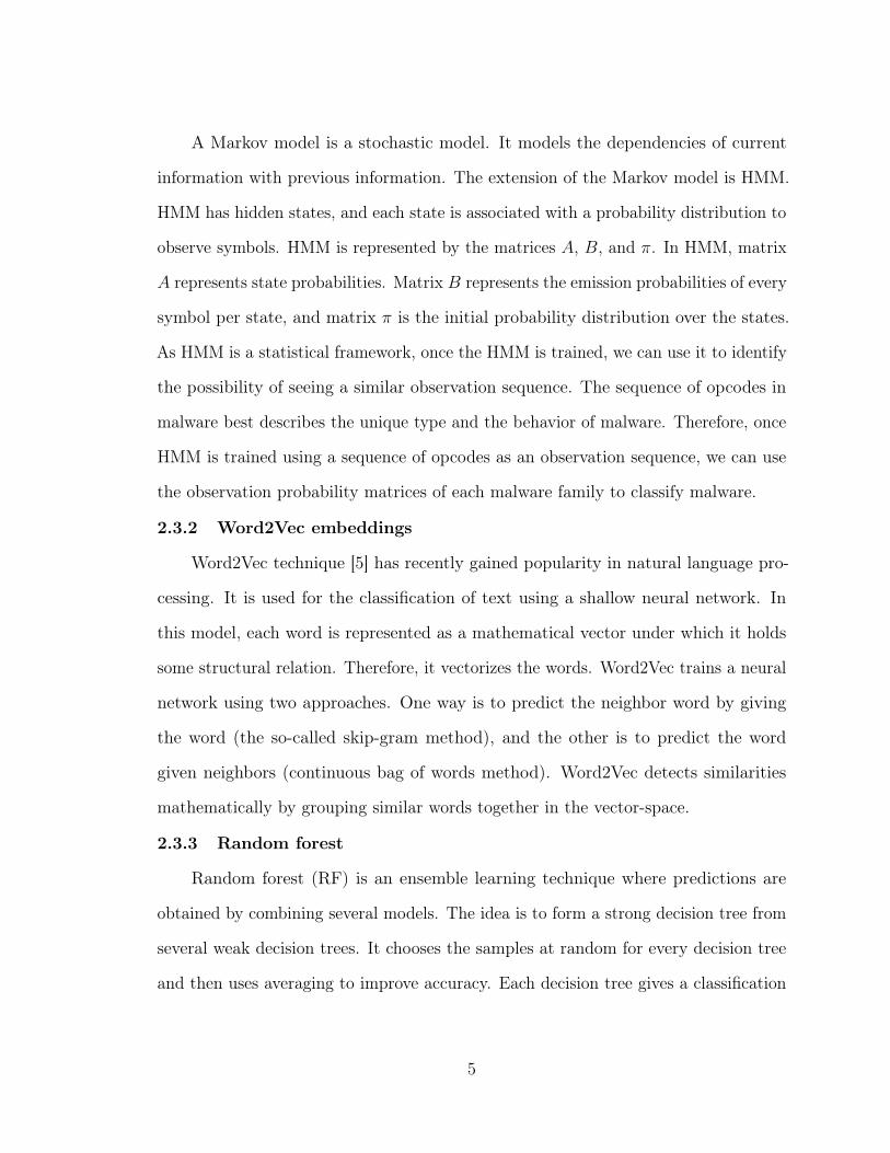
A Markov model is a stochastic model. It models the dependencies of current
information with previous information. The extension of the Markov model is HMM.
HMM has hidden states, and each state is associated with a probability distribution to
observe symbols. HMM is represented by the matrices 𝐴, 𝐵, and 𝜋. In HMM, matrix
𝐴 represents state probabilities. Matrix 𝐵 represents the emission probabilities of every
symbol per state, and matrix 𝜋 is the initial probability distribution over the states.
As HMM is a statistical framework, once the HMM is trained, we can use it to identify
the possibility of seeing a similar observation sequence. The sequence of opcodes in
malware best describes the unique type and the behavior of malware. Therefore, once
HMM is trained using a sequence of opcodes as an observation sequence, we can use
the observation probability matrices of each malware family to classify malware.
2.3.2 Word2Vec embeddings
Word2Vec technique [5] has recently gained popularity in natural language pro-
cessing. It is used for the classification of text using a shallow neural network. In
this model, each word is represented as a mathematical vector under which it holds
some structural relation. Therefore, it vectorizes the words. Word2Vec trains a neural
network using two approaches. One way is to predict the neighbor word by giving
the word (the so-called skip-gram method), and the other is to predict the word
given neighbors (continuous bag of words method). Word2Vec detects similarities
mathematically by grouping similar words together in the vector-space.
2.3.3 Random forest
Random forest (RF) is an ensemble learning technique where predictions are
obtained by combining several models. The idea is to form a strong decision tree from
several weak decision trees. It chooses the samples at random for every decision tree
and then uses averaging to improve accuracy. Each decision tree gives a classification
5

by voting for that class. RF then selects one classification with most of the votes. As
random forest not only bags observations but also the features, it becomes immune to
overfitting, unlike decision trees [11]. A variety of hyperparameters is used to optimize
the performance of RF. The number of decision trees in RF is defined by 𝑛-estimators.
The minimum sample split defines a required number of observations at the tree
node for further division of that node. Increasing the minimum sample split prevents
overfitting. Another hyperparameter in RF is maximum features. Maximum features
can control a list of features before spitting the node in a decision tree of RF. The
minimum sample leaf specifies the minimum number of samples that should be present
at the leaf after a node is split. The hyperparameter maximum depth is the longest
path in a decision tree from root to leaf. Setting this parameter helps in limiting the
height of a tree, therefore avoids overfitting. When bootstrap hyperparameter is set to
false, the entire dataset is used to build the RF. All the mentioned hyperparameters
can be tuned to improve the performance of RF.
2.3.4 𝑘-nearest neighbors (𝑘NN)
Perhaps the most straightforward supervised machine learning algorithm possible
is 𝑘NN. 𝑘NN technique does not make any assumptions related to data distribution. It
is a lazy classifier that classifies the data based on similarity measures using distance
functions. 𝑘NN is used in pattern recognition and statistical estimations [12]. It
classifies the data in two stages. In the first stage, 𝑘-neighbors are determined. In
the second stage, the class of a given sample is determined based on the results of 𝑘
selected neighbors. The ideal value of 𝑘 is dependent on the nature of the data. As 𝑘
increases, accuracy reduces, and the classification boundaries become less distinct.
6

2.3.5 Support vector machine
Support vector machine [13], a supervised machine learning algorithm, analyzes
and identifies the pattern in the data to perform classification. In [14], the authors
claim that SVMs perform well on malware classification problems using 𝑛-gram of
byte codes as the feature. It uses linear classifiers, using a vector of weights 𝑤 and
intercept 𝑏. SVM is based on three concepts.
• Hyperplane: Hyperplane separates the input data into two classes. If the number
of classes is 𝑋, then the hyperplane has 𝑋 − 1 dimensions.
• Hyperparameters to maximize the margin: To classify data samples, we need
a hyperplane with the largest minimum margin with maximum accuracy. It
can be achieved by tuning two regularization parameters, which are 𝐶 and
𝛾. The hyperparameter 𝐶 is known as the cost parameter. It trades off the
misclassification of data against the decision surface. When a model selects
samples as support vectors, 𝛾 is the inverse of the radius of influence of those
samples. Large values of 𝛾 determine if two samples that are very close to each
other are similar or not. On the other hand, small values of 𝛾 means the two
samples are considered similar even if they are far from each other. That is, 𝛾
controls the shape of the decision boundary.
• Kernel trick: The data is transformed into the higher dimensional space using a
kernel function where the hyperplane separates data into classes. The two most
common kernel functions used are radial basis kernel function (RBF) and linear
kernel.
2.3.6 Deep neural network
Neural network (NN) is a collection of algorithms that resembles the structure
of the human brain. DNN is derived from NN, where neuron layers are hidden.
7

The complex structure of DNN makes it learn the abstract features automatically.
Researchers widely use DNN for natural language processing, image recognition, and
pattern recognition. A convolutional neural network (CNN) is one of the DNNs. It is
known for image classification problems. The architecture of CNN consists of hidden
layers, input, and output layers. Hidden layers of CNN include the convolutional layer,
fully connected layers, normalization layer, and pooling layers [5].
2.4 Previous work
Machine learning has been widely used to classify malware. This section introduces
different approaches in a selective review of the relevant literature.
In [15], the author suggests that a series of API calls can be used as a feature to
identify malware. Different features such as opcodes [16], system calls, control flow
graphs, and byte sequences can be used while training machine learning models to
detect malware [14]. When the opcode sequence and their frequencies were used as
features, malware samples were classified accurately. As proposed in [15], the static
analysis of malware by obtaining opcode sequences is efficient and faster as compared
to dynamic analysis techniques.
The authors from [14], proposed to use 𝑛-gram of byte codes as a feature to
classify malware from benign samples. They gathered distinct 𝑛-grams and used
SVM, naive Bayes, term frequency-inverse document frequency (TFIDF) classifier,
and decision trees for classification. The authors claimed that boosted decision trees
achieved the highest accuracy for malware classification with 0.996 as area under the
curve.
The literature discusses many hybrid machine learning techniques for malware
classification. In [17], the author, proposed a hybrid machine learning technique by
using the HMM matrices as the input to a convolutional neural network to classify
8

malware families. Researchers in [17] also used SVM to classify the trained HMMs.
In [18], the author suggested an ensemble model that combines predictions from .asm
and .byte files together after training using xception models. The predictions are
stacked and fed to the neural network for classification. In [19], the authors proposed
to use the Word2Vec technique to generate embeddings from machine instructions.
Moreover, they proposed a proof of concept model to train a convolutional neural
network based on the vectors generated by Word2Vec. This research is highly motivated
by the work in [15], [17], and [19]. We propose hybrid machine learning techniques
using opcode sequences for the classification of malware families. The methods are
discussed in depth in Chapter 3.
9

CHAPTER 3
Implementation
This chapter comprises two sections. The first section gives information about the
dataset used in this research and overview of malware families used for classification.
In the second section, we propose hybrid machine learning techniques.
3.1 Dataset
The raw dataset is used to conduct experiments that involve the classification
of 7 malware families, Winwebsec [20], BHO [21], Renos [22], OnLineGames [23],
Ceeinject [24], Fakerean [25], and Vobfus [26]. The raw dataset has 2793 malware
families that have at least one sample. We decided to generate 1000 HMMs for 7
families. There should be around 1000 executables to train 1000 HMMs. However,
most of the families have less than 100 samples. Therefore, we decided to analyze
50 malware families having the maximum number of samples. Figure 1 shows the
number of samples present in the 50 malware families.
In this research, we train HMMs and Word2Vec models using opcode sequences.
Therefore, data exploration involves identifying the most frequent opcodes from the raw
dataset. In the raw dataset, each malware family has a set of executables. We converted
these executables to .asm files using Linux command objdump. The preprocessing
involved extracting the opcodes from these .asm files. Once we obtained opcode
sequences, we trained HMMs for each malware family using the opcode sequence as
an observation sequence. To select the optimum number of opcodes, we experimented
using 20, 31, and 40 most frequent opcodes based on the opcode distribution in raw
dataset. After deciding the most frequent opcodes, HMM matrices, i.e., 𝐴, 𝐵, and
𝜋, were initialized to approximately 1/𝑁 , 1/𝑀 , and 1/𝑁 per row, respectively. The
number of hidden states is represented by 𝑁 , and the number of output symbols is
represented by 𝑀 . In this research, the number of opcodes is represented by 𝑀 . We
10

Figure 1: Number of samples per family
used 31 frequent opcodes, and the rest of the opcodes were ignored while training
HMMs.
Based on the accuracies and cost of computation, we decided to use the 31 most
frequent opcodes, as shown in Figure 2. Most frequent 20 opcodes contribute to
75.3% of total opcodes. Most frequent 31 opcodes contribute to 83.2% of opcodes,
and most frequent 40 opcodes contribute to 87.2% of total opcodes. Top 30 opcodes
contribute to 82.3% of the total number of opcodes, therefore using 31 opcodes for
these experiments increases opcode contribution percentage by 1. The experiments
11
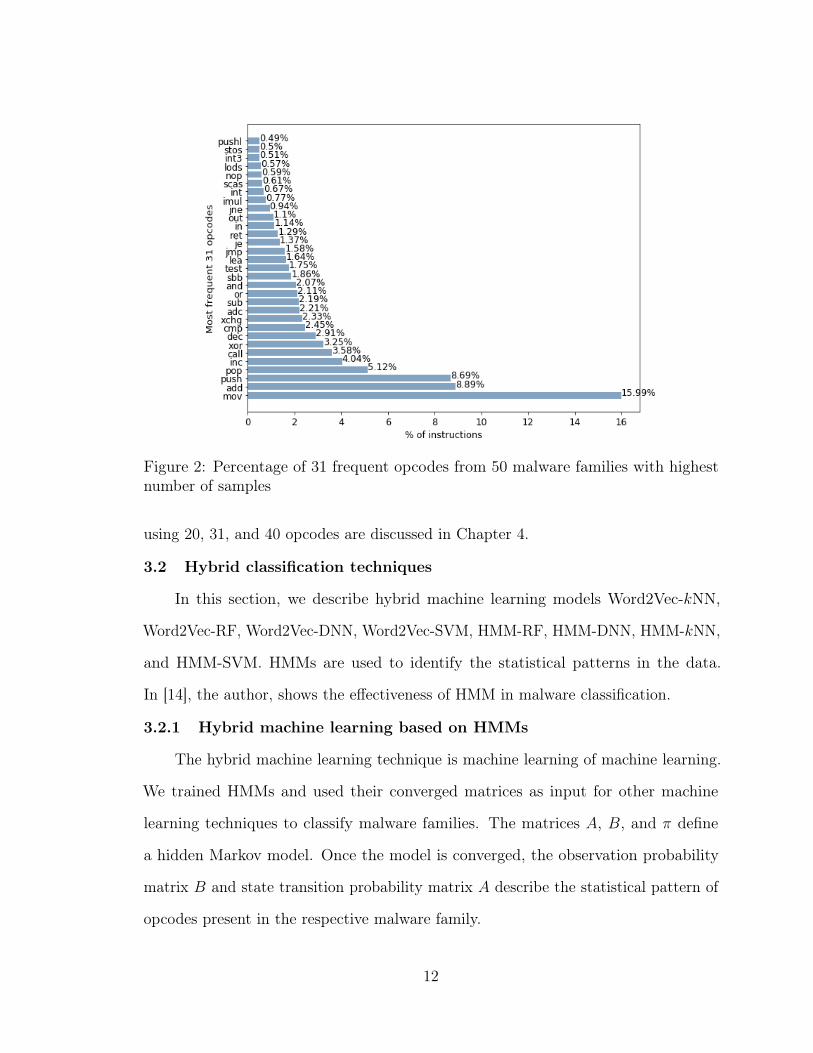
Figure 2: Percentage of 31 frequent opcodes from 50 malware families with highestnumber of samples
using 20, 31, and 40 opcodes are discussed in Chapter 4.
3.2 Hybrid classification techniques
In this section, we describe hybrid machine learning models Word2Vec-𝑘NN,
Word2Vec-RF, Word2Vec-DNN, Word2Vec-SVM, HMM-RF, HMM-DNN, HMM-𝑘NN,
and HMM-SVM. HMMs are used to identify the statistical patterns in the data.
In [14], the author, shows the effectiveness of HMM in malware classification.
3.2.1 Hybrid machine learning based on HMMs
The hybrid machine learning technique is machine learning of machine learning.
We trained HMMs and used their converged matrices as input for other machine
learning techniques to classify malware families. The matrices 𝐴, 𝐵, and 𝜋 define
a hidden Markov model. Once the model is converged, the observation probability
matrix 𝐵 and state transition probability matrix 𝐴 describe the statistical pattern of
opcodes present in the respective malware family.
12

3.2.1.1 HMM-SVM
HMM-SVM is a hybrid machine learning technique that uses converged models
of HMM as features for the SVM technique. We use opcode sequences as features to
train HMMs. The converged matrices are converted to the one-dimensional vectors by
appending each row from the respective matrix. Therefore, the converged observation
probability matrix of HMM will generate one such vector. The output of this task
produces two vectors per converged model; one represents vectors created from 𝐴
matrices and other created from 𝐵 matrices. However, for all the experiments, the
vectors generated from 𝐵 matrices are used as features for training.
3.2.1.2 HMM-RF
The random forest not only bags observations but also features, and unlike
decision trees, the random forest does not overfit data [11]. We propose HMM-RF, a
hybrid machine learning technique, that uses converged matrices of hidden Markov
models as features to random forest algorithm for multiclass malware classification.
In this research, we used an ensemble library from sklearn [27] to implement RF using
Python.
3.2.1.3 HMM-𝑘NN
The 𝑘-nearest neighbors (𝑘NN) algorithm [11] is widely used for classification.
When 𝑘NN is trained, the parameter 𝑘 plays a vital role in classification. The number
of nearest neighbors which are included in the voting process is represented by 𝑘. Low
values of 𝑘 result in overfitting, and large values of 𝑘 underfit the model. Therefore,
we experimented on different values of 𝑘. We propose HMM-𝑘NN, a hybrid machine
learning technique that uses the vectors generated from HMMs to classify a variety of
malware families. The number of neighbors corresponds to the number of malware
families.
13

3.2.1.4 HMM-DNN
Although CNNs are widely used for image classification, we used one-dimensional
CNNs for malware classification because the input is a set of vectors [11]. CNN
identifies structural patterns of malware families, which can classify them. We propose
HMM-DNN, a hybrid machine learning technique, that uses the vectors generated from
HMMs and trained to classify 7 malware families. We experimented using a variety of
parameters such as different numbers of hidden layers, neurons, loss functions, and
optimizers.
3.2.2 Hybrid machine learning based on Word2Vec embeddings
Word2Vec expects a stream of words, which are the sentences in natural language
processing. In our research, the sequence of opcodes, present in malware executables,
is treated as a stream of words. We observe that the vectors of opcodes have small
distances among them when they are semantically close. This property can uniquely
identify peculiar patterns that are unique to malware families. Therefore, we generated
the vectors using Word2Vec and used those for other machine learning algorithms as
input. Each vector is of size 𝑣𝑤, where 𝑣 is a vector size, and 𝑤 is a window size. The
hybrid machine learning models that we propose in this research, Word2Vec-SVM,
Word2Vec-RF, Word2Vec-DNN, and Word2Vec-𝑘NN, learn from the Word2Vec vector
representations of the words by using different vector sizes and window sizes.
14

CHAPTER 4
Results and Analysis
In this chapter, we present the results and analysis of hybrid machine learning
models. We have used opcode sequences as the feature for classification. We focus the
experiments on 8 hybrid machine learning techniques HMM-SVM, HMM-𝑘NN, HMM-
RF, HMM-DNN, Word2Vec-SVM, Word2Vec-RF, Word2Vec-DNN, and Word2Vec-
𝑘NN. After exploring the raw dataset, the next step in malware classification is to
decide the number of opcodes to train models. Therefore, we performed experiments
using different numbers of opcodes to classify two malware families and compared
their accuracies. Later, we added more families for multiclass classification. The first
section of this chapter describes experiments for binary classification. The second
section describes the multiclass malware classification of 7 malware families using 8
hybrid machine learning techniques.
4.1 Binary classification to determine the number of opcodes
In this section, we classified the samples from Winwebsec and Fakerean malware
families, both of which are rogue security softwares that claim to be genuine antivirus
tools and lure the victims into buying illegitimate antivirus software. To decide the
number of opcodes, we evaluated each experiment based on two parameters, i.e., the
time required to generate vectors and accuracy achieved. We compared test accuracies
of experiments based on most frequently occurring 20, 31, and 40 opcodes from the
raw dataset.
4.1.1 Training Word2Vec
We generated 1000 Word2Vec vectors for each family using vector size of 2 and
window sizes of 1, 5, 10, 30, 100. Therefore, for each experiment we used 2000 vectors.
15
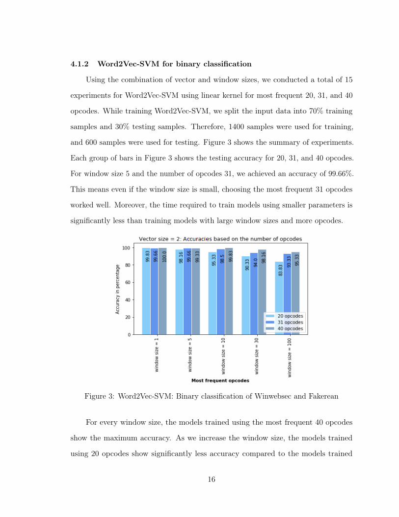
4.1.2 Word2Vec-SVM for binary classification
Using the combination of vector and window sizes, we conducted a total of 15
experiments for Word2Vec-SVM using linear kernel for most frequent 20, 31, and 40
opcodes. While training Word2Vec-SVM, we split the input data into 70% training
samples and 30% testing samples. Therefore, 1400 samples were used for training,
and 600 samples were used for testing. Figure 3 shows the summary of experiments.
Each group of bars in Figure 3 shows the testing accuracy for 20, 31, and 40 opcodes.
For window size 5 and the number of opcodes 31, we achieved an accuracy of 99.66%.
This means even if the window size is small, choosing the most frequent 31 opcodes
worked well. Moreover, the time required to train models using smaller parameters is
significantly less than training models with large window sizes and more opcodes.
Figure 3: Word2Vec-SVM: Binary classification of Winwebsec and Fakerean
For every window size, the models trained using the most frequent 40 opcodes
show the maximum accuracy. As we increase the window size, the models trained
using 20 opcodes show significantly less accuracy compared to the models trained
16

using 40 opcodes. If we add more malware families, the accuracy reduces further. The
models trained using the most frequent 31 opcodes show better accuracy than models
trained using 20 opcodes. The difference between the accuracies of models trained
using 31 opcodes and 40 opcodes is not significant. Moreover, training HMMs using
40 most frequent opcodes costs more computational resources than training HMMs
using 31 most frequent opcodes. To reap both the benefits of less computational time
and better testing accuracy, we decided to choose the most frequent 31 opcodes for
hybrid machine learning techniques for the classification of 7 malware families.
4.2 Multiclass malware classification
This section describes the experiments for multiclass classification. We have
obtained the results using 8 different hybrid machine learning models.
We used 7 malware families namely Winwebsec [20], BHO [21], Renos [22],
OnLineGames [23], Ceeinject [24], Fakerean [25], and Vobfus [26] for all hybrid
machine learning experiments.
We obtained the most frequent 31 opcodes from 50 malware families with a
maximum number of samples and ignored the rest of the opcodes while training
HMMs.
4.2.1 Training HMMs
As part of this experiment, each HMM model was initialized as follows: 𝑁 = 2,
𝑀 = 31. The number of opcodes is represented by 𝑀 . For these classification
experiments, 𝑁 is set to 2 as it gives best classification [28] and 𝑛-grams is set to 1.
To train these HMMs, we used the hmmlearn library [29]. The best model is
obtained after 100 random restarts. The malware samples in this dataset contain
opcode sequences of length more than 50000. The best model was obtained after 100
random restarts for a sequence of opcodes if the length of the observation sequence
17

is between 1000 to 5000 opcodes. Otherwise, the best model was selected after 50
random restarts. The rest of the models were discarded. Any opcode which is not the
part of the top 31 opcodes is discarded. Therefore, it is not counted in 𝑀 . Converged
matrices of the best model are converted to a one-dimensional vector by appending
each row of the matrix one after the other. Moreover, while generating the vectors,
we made sure to assign the probabilities to predefined positions for each opcode. We
created two vectors, each from the matrix 𝐴 and 𝐵 for every HMM. In this research,
we conducted all the experiments by using vectors generated from 𝐵 matrices.
4.2.2 HMM-SVM
This section discusses experiments using different kernel functions for classifica-
tion. For HMM-SVM, we used one-dimensional vectors obtained from 𝐵 matrices of
converged HMMs.
4.2.2.1 HMM-SVM using linear kernel
Figure 4 represents the accuracy of the HMM-SVM model that classifies 7 malware
families, namely BHO, OnLineGames, Renos, Winwebsec, Fakerean, Vobfus, and
Ceeinject. Different values of hyperparameter, 𝐶, were used to analyze the accuracies.
The six values of 𝐶 used are 0.001, 0.01, 0.1, 1, 10, and 100. The best accuracy using
a linear kernel was 0.89 for 𝐶=100.
According to Figure 5, the percentage accuracy of predicting the malware samples
from BHO and Vobfus is highest which is 94.2% and 96.6% respectively. The percentage
accuracy of predicting the malware samples from Winwebsec and Fakerean is lowest.
Figure 5 shows that 9% of testing samples from Winwebsec are misclassified as Fakerean
and 7% of testing samples from OnLineGames are misclassified as Fakerean.
18

Figure 4: HMM-SVM, Accuracy vs 𝐶
Figure 5: Confusion matrix for HMM-SVM with linear kernel
4.2.2.2 HMM-SVM using grid search
To find the best suitable hyperparameters, we tried a different combination of 𝐶
and 𝛾 with linear and RBF kernels. Similar to the exhaustive grid search method [30],
19

we randomly pick 70% of the total number of input vectors for training and 30% of
the total number of input vectors for testing. We obtained a variety of accuracies for
HMM-SVM using linear and RBF kernels.
Table 1: HMM-SVM accuracies
Kernel 𝐶 𝛾 Accuracylinear 1 — 0.83linear 10 — 0.87linear 100 — 0.88linear 1000 — 0.88RBF 1 0.001 0.13RBF 1 0.0001 0.13RBF 10 0.001 0.42RBF 10 0.0001 0.13RBF 100 0.001 0.69RBF 100 0.0001 0.34RBF 1000 0.001 0.83RBF 1000 0.0001 0.70
Table 1 lists all the accuracies that we obtained from grid search. We can notice
that the model with 𝐶 = 100 gave the best accuracy when we used a linear kernel.
However, the RBF kernel is not suitable for malware classification. All in all, it is
clear from the experiments that for HMM-SVM, linear kernel worked well to classify 7
malware families.
4.2.3 HMM-𝑘NN
As 𝑘NN captures the closeness of data samples, in this experiment, we classify
malware based on their similarities. The experiments were conducted with 𝑛-fold
cross-validation and without 𝑛-fold cross-validation with the value of 𝑛 set to 5. The
input for HMM-𝑘NN is a set of vectors, each created by using 𝐵 vectors from HMM
training. A total of 7000 vectors were used. The labeled input vectors are split into
two sections of training and testing data. We randomly pick 70% of the total number
of input vectors for training and 30% vectors for testing. Therefore, 4900 vectors were
20

used for training, and 2100 vectors were used for testing. In, 𝑘NN, 𝑘 is the number of
neighbors that contribute to the voting process to classify malware samples. In this
research, we refer to the number of neighbors as 𝑘-neighbors.
4.2.3.1 HMM-𝑘NN without cross-validation
We performed experiments for different values of neighbors in the range
1, 2, 3, . . . , 100. As we increased the value of 𝑘-neighbors, our predictions achieved
more stability as there is a majority of voters. 𝑘NN is the simplest algorithm and
an optimal value of 𝑘 does not depend on the number of classes. A general rule of
thumb to find the optimal value of 𝑘-neighbors is a square root of training samples.
As we have 4900 samples for training for this experiment, the optimal value of 𝑘 is 70.
Therefore, we are interested in 𝑘NN accuracy when 𝑘-neighbors are 70.
Figure 6: Confusion matrix for HMM-𝑘NN with 𝑘 = 70
21

Figure 6 is a confusion matrix for HMM-𝑘NN when 𝑘 = 70. As shown in Figure 6,
we observe that the percentage accuracies of predicting the malware samples from
BHO, Ceeinject, and Vobfus are the highest. In this technique, we observed the
misclassification similar to HMM-SVM. The samples from Winwebsec are misclas-
sified as Fakrean. Winwebsec is also misclassified as OnLineGames. Samples from
OnLineGames family are misclassified as Fakerean samples. The overall percentage
of misclassification is higher in HMM-𝑘NN. This could be because of the bias in the
data. To avoid this bias, we trained HMM-𝑘NN with cross-validation.
4.2.3.2 HMM-𝑘NN with cross-validation
In this subsection, we trained HMM-𝑘NN with 5-fold cross-validation. We trained
the 𝑘NN classifier for different values of neighbors in the range 𝑘 = 1, 2, 3, . . . , 100. Fig-
ure 7 represents average accuracy for 5-fold cross-validation with varying 𝑘-neighbors,
which was obtained using HMM-𝑘NN to classify 7 malware families.
Figure 7: HMM-𝑘NN, cross-validation: Average accuracy for varying 𝑘-neighbors,using 𝐵 vectors
As shown in Figure 7, as we increased the value of 𝑘-neighbors, our predictions
achieved more stability as there is a majority of voters. As we know that the optimal
22

value of 𝑘 is a square root of training samples. In this experiment, we have 80%
training samples and 20% testing samples. Therefore, we have 5600 training samples
for this experiment. The optimal value of 𝑘-neighbors should be around 75. As it can
be observed in Figure 7, accuracy of predictions decreases as we increase 𝑘-neighbors.
For all the values of 𝑘 before 75, the model overfits the data. From 𝑘=70 to 𝑘=80,
we see a small peak where the accuracy is maximum. We achieved 79% accuracy for
𝑘 = 75 for HMM-𝑘NN when this hybrid model was trained with 𝐵 vectors.
4.2.4 HMM-RF
When it comes to supervised learning, studies have shown that random forests
and neural networks hold a high level of predictive accuracy [31]. We trained HMM-
RF using vectorized versions of the 𝐵 matrices obtained from HMMs. For these
experiments, we have 7000 vectors in total. The training data for HMM-RF involves
splitting the set of vectors into 70% training and 30% testing samples. A random split
is obtained after shuffling the feature vectors. We used 1000 trees in the forest, and
the maximum depth of the tree was set to 300.
Figure 8 represents a confusion matrix obtained for HMM-RF. For HMM-RF,
we obtained an accuracy of 0.949 for multiclass malware classification, which is
highest so far. To further optimize the performance of HMM-RF, we decided to tune
hyperparameters. The best hyperparameters are impossible to find ahead of time.
However, a randomized search can be used to find hyperparameters by providing
a combination of parameters to the model. The best parameters obtained using a
randomized search are shown in Table 2.
Using the parameters mentioned in Table 2, we retrained HMM-RF classifier.
Figure 9 represents a confusion matrix obtained for this experiment, which gives a
visual representation of classification for each malware family. Figure 8 and Figure 9
23

Figure 8: Confusion matrix for HMM-RF
Table 2: Randomized search parameters for HMM-RF
Hyperparameter Value𝑛-estimators 1000
min samples split 2min samples leaf 1
max features automax depth 50bootstrap false
indicate that BHO and Vobfus are 97% and 99% correctly classified. The percentage of
misclassification between malware samples of OnLineGames and Fakerean is reduced
to 4%. Moreover, 4% of testing samples of Winwebsec are getting misclassified as
Fakerean. So overall, we observe the same pattern for malware misclassification, as
observed in HMM-SVM.
24

Figure 9: Confusion matrix for HMM-RF using grid parameters
Figure 10: HMM-RF cross-validation, average accuracy across 10 folds
To summarize HMM-RF, the accuracy of 96% was achieved when this hybrid
model was trained on 𝐵 vectors with best-obtained parameters using a randomized
search. It is the highest accuracy obtained so far. We also performed cross-validation
25

for the values of 𝑛-folds as 2, 3, . . . , 10. Figure 10 represents average accuracy over the
set of folds for HMM-RF.
4.2.5 HMM-DNN
To select a model for a classification problem using deep learning (DL), there are
a variety of options, which include one-dimensional (1-D) CNN, two-dimensional (2-D)
CNN, recurrent neural networks (RNN) and so on. As HMM-DNN classification is
based on the 1-D vectors generated from converged HMM matrices where each vector
is of length 200, we chose fully connected DNN, which is equivalent to 1-D CNN.
In DNN, the prediction error is represented by loss. Loss determines the gradient
and gradient defines how far the model is from predicting the correct class. In short,
gradient updates the weights associated with neurons. Loss functions calculate this loss.
There are four most commonly used loss functions, namely mean squared error (MSE),
binary cross-entropy (BCE), categorical cross-entropy (CC), and sparse categorical
cross-entropy (SCC) [32]. In HMM-DNN, we experimented on MSE, CC, SCC loss
functions, and different numbers of fully connected layers and neurons.
We split input data into 80% training samples, 10% validation samples, and 10%
testing samples. With this split, we obtained 5600 training samples, 700 validation
samples, and 700 testing samples. We trained each model using the rectified linear
unit (ReLU) activation layer and 200 epochs. To construct a sequential model, we
used Keras [33] library.
4.2.5.1 Multilayer perceptron: Optimizer selection
In the first experiment, we trained HMM-DNN using one input layer of dimension
200, a hidden layer using 500 neurons and an output layer using 7 neurons as we
have 7 classes. We used MSE as the loss function and stochastic gradient descent
(SDG) as the optimizer. Both training and testing accuracies were 50%, which is as
26

good as a flip of a coin. To achieve better accuracy, we changed the optimizer to
Adam [34] and kept the loss function as MSE. With this change, we achieved training
accuracy of 97% and testing accuracy of 92%. As Adam uses an adaptive learning
strategy, we got better accuracy. We then used Adam for all further experiments.
4.2.5.2 Multilayer perceptron: 2 hidden layers of 20 neurons
We trained HMM-DNN with 2 hidden layers, one input layer, and an output
layer with 20, 200, and 7 neurons, respectively. The output layer has 7 neurons
because we have 7 malware families to classify. We used CC as the loss function. In
this experimental setup, we achieved the best testing accuracy of 88% after varying
hyperparameters. At this point, the model showed a 40% loss. We decided to continue
further experiments using 500 neurons for a hidden layer.
4.2.5.3 Multilayer perceptron: Loss function selection
A grid search method helps to identify the best hyperparameters. However, it is
cost-effective to train a DNN. The other way is to try different values to regularize
a DNN. Therefore, we chose to compare models using different loss functions. Loss
functions CC and SCC work well for classification problems. Therefore, we performed
two more experiments to decide the loss function. In these experiments, we used
one input layer with 200 neurons, one hidden layer with 500 neurons and the ReLU
activation function, and the output layer of 7 neurons followed by softmax activation.
In this setup, we achieved a testing accuracy of 93.7% using the previously mentioned
sparse categorical cross-entropy and 93.8% using CC. Therefore we continued to use
categorical cross-entropy for further experiments. In both cases, the training accuracy
is 100%, which implies overfitting.
Figure 11 shows model accuracy and Figure 12 shows model loss for the experiment
using categorical cross-entropy. As you can see in Figure 11, the gap between training
27

Figure 11: Model accuracy for HMM-DNN — overfitting
Figure 12: Model loss for HMM-DNN — overfitting
accuracy and validation accuracy is reducing, but as per Figure 12, the gap between
validation loss and training loss is increasing. As we increase the number of epochs,
accuracy keeps on increasing; this suggests that the model overfits training data.
4.2.5.4 Multilayer perceptron: Dropout layer
So far, we observed that the HMM-DNN overfitted the data with high loss. There
are a handful of ways to minimize loss. DNN can be regularized using a dropout layer.
Figure 13 shows the DNN architecture with an added dropout layer. It drops out
28

inputs to the layer in a probabilistic manner. We set the dropout rate to 0.5. In this
setup, we achieved a testing accuracy of 94.2% and a training accuracy of 98%. The
training accuracy is reduced, which means that the model is not overfitting.
Figure 13: HMM-DNN model architecture
Figure 14 (a) and (b) shows model accuracy and and loss, respectively, for this
experiment. Training and validation accuracies are increased as we increase the number
of epochs. As shown in Figure 14 (b), the validation loss curve and training loss curve
are more coherent to each other than shown in Figure 12. It means that the model
is not overfitting, unlike before. All in all, HMM-DNN achieved 94% of accuracy to
classify 7 malware families, which is the second-best accuracy achieved for HMM-based
hybrid machine learning models.
4.2.6 Word2Vec-SVM
The experiments conducted in this section use vector embeddings generated
from the Word2Vec algorithm. The generated vectors are analogous to the vectors
generated using HMM. However, Word2Vec gives us the flexibility to choose vector
and window sizes to generate vector embeddings. We used 7 malware families for
this experiment and, therefore, the number of samples for this experiment is 7000.
29

(a) Accuracy (b) Loss
Figure 14: Model accuracy and loss for HMM-DNN
Word2Vec based hybrid machine learning models are also trained using the most
common 31 opcodes. In this section, we discuss three significant experiments we
conducted using Word2Vec-SVM.
4.2.6.1 Word2Vec-SVM using linear kernel
For Word2Vec-SVM, we used a linear kernel with a one-versus-other technique.
We split the input data in 70% training samples and 30% testing samples. We
generated Word2Vec vectors of size 2, 31, 100, and windows of size 1, 5, 10, 30, 100.
Using the combination of vector and window sizes, we conducted 15 experiments for
Word2Vec-SVM using linear kernel.
We achieved 95% accuracy to classify 7 malware families using linear kernel with
input vectors of size 31 and window of size 1. Figure 15 clearly indicates the accuracies.
Figure 15 shows that accuracies significantly improved when the vector size
increased from 2 to 31. We used 31 opcodes for this training, so the vector size 31
worked best for Word2Vec-SVM. We also observed that as window sizes increased
beyond 10, the accuracies reduced.
30

Figure 15: Word2Vec-SVM, linear kernel: Accuracy vs different vector and windowsizes
4.2.6.2 Word2Vec-SVM using grid search
So far, we used a linear kernel for SVM related experiments. To check which
kernel is suitable, we used an exhaustive grid search method [30]. Table 3 represents
grid search parameters obtained after training Word2Vec-SVM for input vectors of
size 2 and window of size 30. We used 𝑛-fold cross-validation for grid search where
𝑛 was 5. As shown in Table 3, we observed that for RBF kernel with 𝛾 = 0.001, we
achieved the highest accuracy.
4.2.6.3 Word2Vec-SVM using RBF kernel
For the RBF kernel, we used 𝐶 = 1000 and 𝛾 = 0.001. The labeled input vectors
are split into two sections of training and testing data. We randomly pick 70% of the
total number of input vectors for training and 30% vectors for testing. Therefore, we
used 4900 vectors for training and 2100 vectors for testing. We generated Word2Vec
vectors of size 2, 31, 100, and windows of size 1, 5, 10, 30, 100. Using the combination
of vector and window sizes, we conducted 15 experiments for Word2Vec-SVM using
RBF kernel.
31

Table 3: Word2Vec-SVM grid search accuracies, vector size = 2 and window size = 30
Kernel 𝐶 𝛾 Accuracylinear 1 — 0.86linear 10 — 0.85linear 100 — 0.85linear 1000 — 0.85RBF 1 0.001 0.87RBF 1 0.0001 0.70RBF 10 0.001 0.91RBF 10 0.0001 0.84RBF 100 0.001 0.92RBF 100 0.0001 0.88RBF 1000 0.001 0.92RBF 1000 0.0001 0.90
We achieved 95% accuracy to classify 7 malware families using RBF kernel with
input vectors of size 31, and windows of sizes 1 and 30. Figure 16 clearly indicates
the accuracies.
Figure 16: Word2Vec-SVM, RBF kernel: Accuracy vs different vector and windowsizes
As we can see from the Figure 16, when the vector size was increased from 2 to
31, the accuracy of classification was slightly improved. Vector size 31 worked best for
this experiment.
32

4.2.7 Word2Vec-RF
In this experiment, we used 7 malware families for classification, namely, BHO,
OnLineGames, Renos, Winwebsec, Fakerean, Vobfus, and Ceeinject. Therefore, the
number of samples for this experiment is 7000. Word2Vec embeddings are given as
input to the RF algorithm.
For this experiment, Word2Vec vectors were generated for vector sizes 2, 31, 100,
and window sizes 1, 5, 10, 30, 100. The number of trees in the forest is called as
𝑛-estimators, which were set to 1000 by default. A total of 4900 samples were used
for training, and 2100 samples were used for testing. Using this setup, we obtained
the results for 15 different experiments using vector sizes and window sizes mentioned
before. The best accuracy to classify 7 malware families using Word2Vec-RF using
vector size as 100 and window size as 30 is 96.2%. The class-wise confusion matrix
is summarized in Figure 17. Figure 17 indicates that almost all malware families
are classified correctly. Winwebsec is misclassified as Fakerean for 3% of the testing
samples.
Additional results for Word2Vec-RF with different window and vector sizes can be
seen in Appendix A. After conducting experiments using default parameters, we then
obtained the best parameters for RF using a grid search method for the embeddings
generated using vector size as 100 and window size as 30. Table 4 summarizes the
best parameters obtained using grid search.
By using the best parameters, we trained Word2Vec-RF for embeddings generated
using a vector size of 100 and a window size of 30. We performed cross-validation
for the values of folds 2, 3, . . . , 10. Figure 18 shows average accuracy for 𝑛-fold cross-
validation. We achieved around 96% accuracy using the best parameters for 6-fold
cross-validation.
33

Figure 17: Word2Vec-RF classification vector size = 100 and window size = 30
Table 4: Randomized search parameters for Word2Vec-RF
Hyperparameter Value𝑛-estimators 1400
min samples split 2min samples leaf 1
max features automax depth 40bootstrap false
4.2.8 Word2Vec-𝑘NN
For this experiment, we considered 7 malware families, namely BHO,
OnLineGames, Renos, Winwebsec, Fakerean, Vobfus, and Ceeinject. As there are 7
families, the total number of vectors used as input for 𝑘NN is 7000. The experiments
were conducted with 𝑛-fold cross-validation and without 𝑛-fold cross-validation.
34
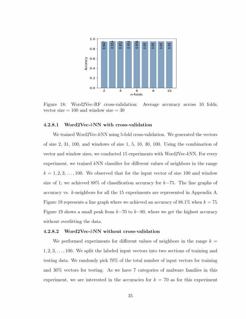
Figure 18: Word2Vec-RF cross-validation: Average accuracy across 10 folds,vector size = 100 and window size = 30
4.2.8.1 Word2Vec-𝑘NN with cross-validation
We trained Word2Vec-𝑘NN using 5-fold cross-validation. We generated the vectors
of size 2, 31, 100, and windows of size 1, 5, 10, 30, 100. Using the combination of
vector and window sizes, we conducted 15 experiments with Word2Vec-𝑘NN. For every
experiment, we trained 𝑘NN classifier for different values of neighbors in the range
𝑘 = 1, 2, 3, . . . , 100. We observed that for the input vector of size 100 and window
size of 1; we achieved 88% of classification accuracy for 𝑘=75. The line graphs of
accuracy vs. 𝑘-neighbors for all the 15 experiments are represented in Appendix A.
Figure 19 represents a line graph where we achieved an accuracy of 88.1% when 𝑘 = 75.
Figure 19 shows a small peak from 𝑘=70 to 𝑘=80, where we get the highest accuracy
without overfitting the data.
4.2.8.2 Word2Vec-𝑘NN without cross-validation
We performed experiments for different values of neighbors in the range 𝑘 =
1, 2, 3, . . . , 100. We split the labeled input vectors into two sections of training and
testing data. We randomly pick 70% of the total number of input vectors for training
and 30% vectors for testing. As we have 7 categories of malware families in this
experiment, we are interested in the accuracies for 𝑘 = 70 as for this experiment
35

Figure 19: Word2Vec-𝑘NN cross-validation: Average accuracy for varying 𝑘-neighbors,vector size = 100 and window size = 1
we have 4900 samples for training. As mentioned in above, we achieved the best
accuracy of 88.1% for Word2Vec-𝑘NN when vector size and window size was 100 and
1, respectively. Therefore, for this experiment, we used vector size as 100 and window
size as 1. The reason to perform this experiment without cross-validation is to see the
classification of an individual malware family.
Figure 20 shows confusion matrix for classification of malware families using
Word2Vec-𝑘NN for 𝑘-neighbors = 70. As we increase the value of 𝑘-neighbors, our
predictions achieve more stability as there is a majority of voters. Figure 20 indicates
that malware samples from BHO, Vobfus, and Fakerean families are correctly classified.
We still see the misclassification of Winwebsec samples as Fakerean samples.
4.2.9 Word2Vec-DNN
We generated Word2Vec vectors using vector sizes of 2, 31, 100, and window
sizes of 1, 5, 10, 30, 100 for each family. With these vectors, we conducted 15
experiments. We used DNN architecture, as shown in Figure 13, to train Word2Vec-
DNN experiments. However, the input layer changes in each experiment, depending
on the vector size.
36

Figure 20: Confusion matrix for Word2Vec-𝑘NN for 𝑘-neighbors = 7, vector size = 100and window size = 1
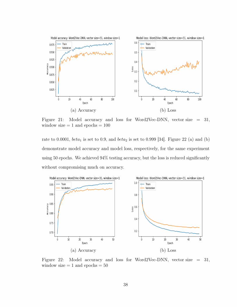
When the training process is going well, loss decreases. Figure 21 (a) and (b),
respectively, demonstrate model accuracy and model loss for one of the experiments
with 31 as vector size, 1 as window size and 200 epochs.
We achieved 95% of testing accuracy with higher loss. If the loss is decreasing,
then the training process is going as per expectations. However, Figure 21 (b) shows
that validation loss increased as the number of epochs increased, and accuracy remains
the same. It means that the model is highly confident about its prediction, and any
misclassification of malware families induces high loss, and the model is diverging.
One of the ways to stop this problem is early stopping. It prevents the waste of
computational resources. Another way is to tune the learning rate. Therefore, as we
increased the window sizes, we reduced the number of epochs to 50, tuned the learning
37
(a) Accuracy (b) Loss
Figure 21: Model accuracy and loss for Word2Vec-DNN, vector size = 31,window size = 1 and epochs = 100
rate to 0.0001, 𝑏𝑒𝑡𝑎1 is set to 0.9, and 𝑏𝑒𝑡𝑎2 is set to 0.999 [34]. Figure 22 (a) and (b)
demonstrate model accuracy and model loss, respectively, for the same experiment
using 50 epochs. We achieved 94% testing accuracy, but the loss is reduced significantly
without compromising much on accuracy.
(a) Accuracy (b) Loss
Figure 22: Model accuracy and loss for Word2Vec-DNN, vector size = 31,window size = 1 and epochs = 50
38

Figure 23 shows the confusion matrix for the classification. It shows that malware
family Fakerean is getting misclassified with OnLineGames and Winwebsec, which is
a common pattern that we have observed so far in all the experiments.
Figure 23: Confusion matrix: vector size = 31, window size = 1 and epochs = 15
Figure 24 indicates a summary of all the 15 experiments we conducted using
Word2Vec-DNN. Each bar represents testing accuracy, number of epochs, window size,
and vector size used. It is clear from the experiment that as we increased the window
size, we decreased the number of epochs to minimize model loss. All in all, the best
accuracy we achieved using Word2Vec-DNN is 94%.
The experiments with 7 malware families show that malware classification gets
more challenging as the model becomes generic. From the experiments, we conclude
that detecting malware using RF and SVM for hybrid machine learning are the most
39

Figure 24: Accuracies across all Word2Vec-DNN experiments
reliable techniques when opcode sequences are used as features. Moreover, hybrid
models based on Word2Vec embeddings obtained better accuracies than HMM-based
models. Word2Vec-RF resulted in 96% accuracy for the classification of 7 malware
families.
4.3 Robustness analysis of hybrid machine learning techniques
Advanced types of malware such as polymorphic malware changes itself constantly
to evade malware detection techniques. One way to evade malware detection algorithms
is to add dead code into malware code from legitimate computer programs. Adding
dead code changes the signature of malware making them difficult to detect. In this
research, to check how robust hybrid techniques are, we scrambled a percentage of
the opcode sequence before training HMM and Word2Vec techniques. For robustness
experiments, we randomly scrambled 10%, 20%, 30%, and 40% of opcode sequences
and trained HMM and Word2Vec to generate the vectors for two malware families,
Winwebsec and Fakerean. We used the most frequent 31 opcodes for all robustness
experiments.
40

4.3.1 Robustness of HMM-based techniques
For all HMM-based experiments, we first generated vectors without any scrambling
of opcodes. We used B matrices from 1000 converged HMM models to generate 1-D
vectors. As we trained all the classifiers using two families, we have a total of 2000
vectors. We trained a binary classifier using HMM-SVM, HMM-𝑘NN, HMM-RF, and
HMM-DNN. Now, we scrambled 10%, 20%, 30%, and 40% of opcode sequences and
generated 300 vectors from 300 HMMs for each percentage of scrambled opcodes. We
did this for Winwebsec and Fakerean families. Now that we have 600 obfuscated
vectors, we tested them on the trained binary classifier. This section describes the
result obtained after scrambling the opcodes.
Figure 25: Robustness experiment for HMM-based hybrid machine learning techniques
In the Figure 25, we show a plot of accuracies vs. a percentage of opcodes that
are scrambled. The accuracies are for the classification of Winwebsec and Fakerean
samples. Each line graph indicates a hybrid machine learning technique. HMM-
DNN shows good tolerance for the scrambled opcodes. The accuracy of HMM-SVM
drastically dropped when tested on 600 samples of obfuscated data. The accuracies of
HMM-𝑘NN and HMM-RF remained between 50% to 60%.
41

4.3.2 Robustness of Word2Vec-based techniques
For all Word2Vec-based experiments, we first generated vectors with vector size
of 2 and window sizes of 1, 5, 10, 30 and 100, without any scrambling of opcodes. We
generated 1000 vector embeddings using Word2Vec model for Winwebsec and Fakerean
malware family. Thus, we have a total of 2000 vector embeddings. We trained binary
classifiers using SVM, 𝑘NN, RF, and DNN. Now, we scrambled 10%, 20%, 30%, and
40% of opcode sequences and generated 600 vectors for each percentage of scrambled
opcodes. We chose 300 vectors from Winwebsec family and 300 vectors from Fakerean
family for that purpose. We tested 600 obfuscated vectors of two families on the
trained binary classifier. This section describes the result obtained after scrambling
the opcodes.
Figure 26: Robustness experiment for Word2Vec-SVM
In Figure 26, we show a plot of accuracies vs. percentage of opcodes that are
scrambled and tested on Word2Vec-SVM model. Each line graph indicates a specific
vector size and window size configuration used for testing the data. As the window
size increased, the accuracy dropped. When the window sizes are 30 and 100, the
accuracies remain in range 50% to 60%. However, for the window sizes of 1, 5, 10,
42

the accuracies remain in the range 60% to 70%. The reason is that, large window
sizes capture more information about the opcode sequence. The vector is affected by
consecutive opcodes. As we have randomly scrambled opcodes, the vectors with large
window sizes add more noise into the vectors making the classification difficult.
Figure 27: Robustness experiment for Word2Vec-𝑘NN
In Figure 27, we show a plot of accuracies vs. percentage of opcodes that
are scrambled and tested on Word2Vec-𝑘NN model. Each line graph indicates a
specific vector size and window size configuration used for testing the data. When
the window sizes are 30 and 100, the accuracies drop to 60% when the percentage
of scrambling opcodes is 40%. As we have randomly scrambled opcodes, the vectors
with large window sizes add more noise into the vectors making the classification
difficult. Moreover, as per Figure 27, vectors generated with window sizes 5 and 10
are comparatively tolerant to the scrambling and the accuracies remain 70%.
In Figure 28, we show a plot of accuracies vs. percentage of opcodes that are
scrambled and tested on Word2Vec-RF model. Each line graph indicates a specific
vector size and window size configuration used for testing the data. When the window
sizes are 30 and 100, the accuracies drop. When the window size is 100, accuracy
43

Figure 28: Robustness experiment for Word2Vec-RF
drops below 50% when a percentage of scrambling is 40. Vectors with window sizes 1,
5, and 10 remain in a range of 60% and 70% accuracies.
Figure 29: Robustness experiment for Word2Vec-DNN
In Figure 29, we show a plot of accuracies vs. percentage of opcodes that are
scrambled and tested on Word2Vec-DNN model. Each line graph indicates a specific
vector size and window size configuration used for testing the data. For Word2Vec-
DNN, we see the same pattern. As we increase the window sizes and percentage of
opcode scrambling, the prediction accuracies keep getting worse.
44

From these obfuscation experiments, we can see that Word2Vec-based hybrid
machine learning technique is robust at different percentages of opcode scrambling
if the window sizes are 1, 5, and 10. Also, HMM-DNN technique is the most robust
at different percentages of opcode scrambling. Chapter 5 discusses the summary and
accuracies in detail.
45

CHAPTER 5
Conclusion and Future Work
In the first set of experiments, we tested hybrid machine learning techniques to
decide the number of opcodes to train our base models, namely HMM and Word2Vec.
In the second set of experiments, we tested the performance of 8 different hybrid
machine learning techniques for malware classification of 7 malware families.
Figure 30 summarizes the best accuracies for Word2Vec-based and HMM-based
hybrid machine learning techniques. HMM-based techniques are trained using 𝐵
vectors of converged HMMs. It is clear from Figure 30 that HMM-RF outperformed all
the models and achieved 96% accuracy to classify 7 malware families. Its configuration
was set to 1000 𝑛-estimators, 50 maximum depth, 1 minimum samples at leaves,
2 minimum samples split, and bootstrap set to false. HMM-DNN also performs
well to classify malware families. Almost all the hybrid machine learning techniques
based on Word2Vec embeddings have performed well. We achieved 96.2% accuracy
for the Word2Vec-RF and 95% accuracy for the Word2Vec-SVM model using both
linear and RBF kernels. In this research, we also performed experiments to test the
robustness of hybrid machine learning models. From the obfuscation experiments, we
concluded that Word2Vec-based hybrid machine learning techniques are robust at
different percentages of opcode scrambling for window sizes less than 30.
Almost all the hybrid machine learning techniques correctly classified the testing
samples from BHO, Vobfus, and Renos. We observed that the samples from Winwebsec
were often misclassified as Fakerean samples. Similarly, the samples from OnLineGames
were often misclassified as Fakerean samples. The percentage of this misclassification
is higher in HMM-based classification techniques than Word2Vec-based classification
techniques.
The substantial advantage of using Word2Vec is its high-speed training time.
46

Figure 30: Best accuracies for HMM-based hybrid machine learning
While HMM models generate 1000 vectors, based on 31 opcodes, in 76 hours, the
Word2Vec model takes 5 hours to do the same. Therefore, it becomes a suitable
method of training when more malware families are added for multiclass classification.
In conclusion, we observed that Word2Vec-based machine learning techniques not
only performed better than HMM-based machine learning techniques but also took
significantly less computational resources to generate the vectors and to train the
hybrid models.
As part of future extension to this research, similar experiments could be performed
on 25 or more malware families. The malware families that are similar to each other
can also be used for future experiments to make the classification more challenging.
In this research, opcode sequences were used as the feature for training HMMs and
generating Word2Vec embeddings. Similarly, corresponding experiments could be
conducted by using the byte 𝑛-gram [35] of opcodes as the feature. As discussed in [15],
47

dynamic features of malware such as API calls could be used to classify malware
families. API calls identify if the sample belongs to a particular malware family based
on the likelihood of the observation sequence used in HMM. Therefore, we could also
train our hybrid models to classify malware families using API calls as a feature.
Instead of building the sequential layers for CNNs, we could also try to use
architectures such as ResNet and VGG [36] by using transfer learning techniques. In
transfer learning, models are pre-trained on a large dataset of images. We could leverage
such well-trained models for malware classification. Moreover, it would be interesting
to combine HMM and Word2Vec features with the Expectation-Maximization (EM)
clustering techniques [37] for the classification.
For this research, we have used a limited number of windows and vector sizes
to generate Word2Vec embeddings. Further experiments could be conducted by
generating a different set of window sizes and vector sizes as the input for our hybrid
machine learning techniques. Another experiment we can try is to create a pipeline of
three or more machine learning algorithms similar to the hybrid models that we have
proposed.
48

LIST OF REFERENCES
[1] J. Aycock, Computer Viruses and Malware. Springer, New York, 2006, vol. 22.
[2] C. Beek, T. Dunton, J. Fokker, S. Grobman, T. Hux, T. Polzer, M. R. Lopez,T. Roccia, J. Saavedra-Morales, R. Samani, and R. Sherstobitof, “McAfee labsthreats report,” https://www.mcafee.com/enterprise/en-us/assets/reports/rp-quarterly-threats-aug-2019.pdf, August 2019.
[3] I. Santos, F. Brezo, J. Nieves, Y. K. Penya, B. Sanz, C. Laorden, and P. G.Bringas, “Idea: Opcode-sequence-based malware detection,” in InternationalSymposium on Engineering Secure Software and Systems. Springer, 2010, pp.35–43.
[4] D. Dhanasekar, F. Di Troia, K. Potika, and M. Stamp, “Detecting encrypted andpolymorphic malware using hidden Markov models,” in Guide to VulnerabilityAnalysis for Computer Networks and Systems: An Artificial Intelligence Approach.Springer, 2018, pp. 281–299.
[5] T. Mikolov, K. Chen, G. S. Corrado, and J. Dean, “Efficient estimation of wordrepresentations in vector space,” https://arxiv.org/abs/1301.3781, 2013.
[6] P. Li, Z. Chen, and B. Cui, “Detecting malware based on opcode n-gram andmachine learning,” in International Conference on P2P, Parallel, Grid, Cloudand Internet Computing. Springer, 2017, pp. 99–110.
[7] M. Ijaz, M. H. Durad, and M. Ismail, “Static and dynamic malware analysis usingmachine learning,” in 2019 16th International Bhurban Conference on AppliedSciences and Technology (IBCAST), 2019, pp. 687–691.
[8] M. F. Zolkipli and A. Jantan, “A framework for malware detection using combina-tion technique and signature generation,” in 2010 Second International Conferenceon Computer Research and Development, 2010, pp. 196–199.
[9] S. Shaily and V. Mangat, “The hidden Markov model and its application tohuman activity recognition,” in 2015 2nd International Conference on RecentAdvances in Engineering Computational Sciences (RAECS), 2015, pp. 1–4.
[10] A. Krogh, M. Brown, I. Mian, K. Sjölander, and D. Haussler, “Hidden Markovmodels in computational biology: Applications to protein modeling,” Journal ofMolecular Biology, vol. 235, no. 5, pp. 1501–1531, 1994.
[11] M. Stamp, Introduction to Machine Learning with Applications in InformationSecurity, 1st ed. Chapman and Hall CRC, 2017.
49

[12] T. K. Hazra, D. P. Singh, and N. Daga, “Optical character recognition usingkNN on custom image dataset,” in 2017 8th Annual Industrial Automationand Electromechanical Engineering Conference (IEMECON). IEEE, 2017, pp.110–114.
[13] C. Cortes and V. Vapnik, “Support-vector networks,” Machine Learning, vol. 20,no. 3, pp. 273–297, 1995.
[14] J. Z. Kolter and M. A. Maloof, “Learning to detect and classify maliciousexecutables in the wild,” Journal of Machine Learning Research, vol. 7, pp. 2721–2744, 2006. [Online]. Available: http://doi.acm.org/10.1145/1014052.1014105
[15] S. Vemparala, F. D. Troia, C. A. Visaggio, T. H. Austin, and M. Stamp,“Malware detection using dynamic birthmarks,” in Proceedings of the 2016ACM on International Workshop on Security And Privacy Analytics, R. M.Verma and M. Rusinowitch, Eds. ACM, 2016, pp. 41–46. [Online]. Available:https://doi.org/10.1145/2875475.2875476
[16] W. Wong and M. Stamp, “Hunting for metamorphic engines,” Journalin Computer Virology, vol. 2, pp. 211–229, 11 2006. [Online]. Available:https://doi.org/10.1007/s11416-006-0028-7
[17] A. Sethi, “Classification of malware models,” 2019. [Online]. Available:https://doi.org/10.31979/etd.mrqp-sur9
[18] W. W. Lo, X. Yang, and Y. Wang, “An xception convolutional neural network formalware classification with transfer learning,” in 2019 10th IFIP InternationalConference on New Technologies, Mobility and Security (NTMS), 2019, pp. 1–5.
[19] I. Popov, “Malware detection using machine learning based on word2vec embed-dings of machine code instructions,” in 2017 Siberian Symposium on Data Scienceand Engineering (SSDSE), 2017, pp. 1–4.
[20] “Win32/Winwebsec threat description - Microsoft security intelligence.”[Online]. Available: https://www.microsoft.com/en-us/wdsi/threats/malware-encyclopedia-description?Name=Win32%2FWinwebsec
[21] “Trojan:Win32/BHO.BO - Microsoft security intelligence.” [Online]. Avail-able: https://www.microsoft.com/en-us/wdsi/threats/malware-encyclopedia-description?Name=Trojan:Win32/BHO.BO
[22] “Win32/Renos threat description - Microsoft security intelligence.” [Online]. Avail-able: https://www.microsoft.com/en-us/wdsi/threats/malware-encyclopedia-description?Name=Win32%2FRenos
50

[23] “Trojan:Win32/OnLineGames.A - Microsoft security intelligence.” [Online]. Avail-able: https://www.microsoft.com/en-us/wdsi/threats/malware-encyclopedia-description?Name=Trojan:Win32/OnLineGames.A
[24] “VirTool:Win32/CeeInject - Microsoft security intelligence.” [Online]. Avail-able: https://www.microsoft.com/en-us/wdsi/threats/malware-encyclopedia-description?Name=VirTool%3AWin32%2FCeeInject
[25] “Rogue:Win32/FakeRean - Microsoft security intelligence.” [Online]. Avail-able: https://www.microsoft.com/en-us/wdsi/threats/malware-encyclopedia-description?Name=Rogue:Win32/FakeRean&threatId=124161
[26] “Win32/Vobfus - Microsoft security intelligence.” [Online]. Avail-able: https://www.microsoft.com/en-us/wdsi/threats/malware-encyclopedia-description?name=win32%2Fvobfus
[27] F. Pedregosa, G. Varoquaux, A. Gramfort, V. Michel, B. Thirion, O. Grisel,M. Blondel, P. Prettenhofer, R. Weiss, V. Dubourg, J. Vanderplas, A. Passos,D. Cournapeau, M. Brucher, M. Perrot, and E. Duchesnay, “Scikit-learn: Machinelearning in Python,” Journal of Machine Learning Research, vol. 12, pp. 2825–2830, 2011.
[28] R. Gonsalves, “A study on effects of data poisoning on hmms,” https://doi.org/10.31979/etd.ezz5-rvrv, 2018.
[29] V. Gael, “hmmlearn,” https://github.com/hmmlearn/hmmlearn, 2014.
[30] Taijia Xiao, Dong Ren, Shuanghui Lei, Junqiao Zhang, and Xiaobo Liu, “Basedon grid-search and pso parameter optimization for support vector machine,” inProceeding of the 11th World Congress on Intelligent Control and Automation,2014, pp. 1529–1533.
[31] R. Caruana and A. Niculescu-Mizil, “An empirical comparison of supervisedlearning algorithms,” in ICML 2006 - Proceedings of the 23rd InternationalConference on Machine Learning, vol. 2006, 2006, pp. 161–168.
[32] J. Brownlee, “How to choose loss functions when training deep learning neuralnetworks,” https://machinelearningmastery.com/how-to-choose-loss-functions-when-training-deep-learning-neural-networks/, 2019.
[33] F. Chollet, “Keras,” https://github.com/fchollet/keras, 2015.
[34] Z. Zhang, “Improved Adam optimizer for deep neural networks,” in 2018IEEE/ACM 26th International Symposium on Quality of Service (IWQoS), 2018,pp. 1–2.
51

[35] R. Zak, E. Raff, and C. Nicholas, “What can n-grams learn for malware detection?”in 2017 12th International Conference on Malicious and Unwanted Software(MALWARE), 2017, pp. 109–118.
[36] K. He, X. Zhang, S. Ren, and J. Sun, “Deep residual learning for image recognition,”in 2016 IEEE Conference on Computer Vision and Pattern Recognition (CVPR),2016, pp. 770–778.
[37] M. Mohammadi and A. Hamzeh, “Proposing an efficient approach for malwareclustering,” in 2017 Artificial Intelligence and Signal Processing Conference(AISP), 2017, pp. 262–267.
[38] A. Nappa, M. Z. Rafique, and J. Caballero, “The malicia dataset:identification and analysis of drive-by download operations,” InternationalJournal of Information Security, vol. 14, 2014. [Online]. Available:http://dx.doi.org/10.1007/s10207-014-0248-7
52
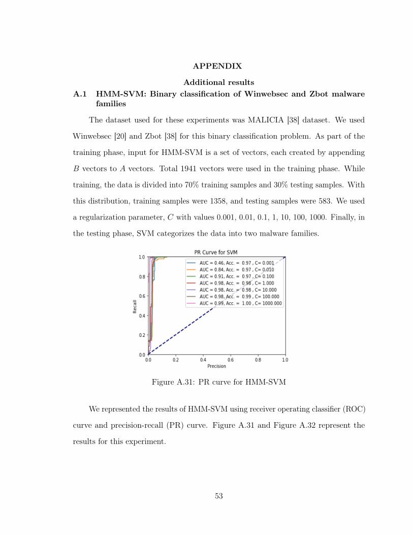
APPENDIX
Additional resultsA.1 HMM-SVM: Binary classification of Winwebsec and Zbot malware
families
The dataset used for these experiments was MALICIA [38] dataset. We used
Winwebsec [20] and Zbot [38] for this binary classification problem. As part of the
training phase, input for HMM-SVM is a set of vectors, each created by appending
𝐵 vectors to 𝐴 vectors. Total 1941 vectors were used in the training phase. While
training, the data is divided into 70% training samples and 30% testing samples. With
this distribution, training samples were 1358, and testing samples were 583. We used
a regularization parameter, 𝐶 with values 0.001, 0.01, 0.1, 1, 10, 100, 1000. Finally, in
the testing phase, SVM categorizes the data into two malware families.
Figure A.31: PR curve for HMM-SVM
We represented the results of HMM-SVM using receiver operating classifier (ROC)
curve and precision-recall (PR) curve. Figure A.31 and Figure A.32 represent the
results for this experiment.
53

Figure A.32: ROC curve for HMM-SVM
A.2 HMM-𝑘NN: Binary classification of Winwebsec and Zbot malwarefamilies
The experiments were conducted with 𝑛-fold cross-validation with the value of 𝑛
set to 5. The input for HMM-𝑘NN is a set of vectors, each created by appending 𝐵
vectors to 𝐴 vectors.
Figure A.33: Mean score of cross-validation vs 𝑘-neighbors
A total of 1940 vectors were used for this hybrid model. Cross-validation shuffles
the data and splits it into 𝑛-folds. Figure A.33 shows the graph of average accuracy
54

for cross-validation vs 𝑘-neighbors. It is clear that using 𝑛-fold cross-validation, we
achieved around 96% accuracy for 𝑘 = 39 as we removed the bias from the data. The
optimal value of 𝑘 is selected as 39 based on the number of training samples.
A.3 Word2Vec-RF: Multiclass classification
The Table A.5 shows the accuracies of Word2Vec-RF malware classification of 7
malware families for vector sizes and window sizes.
Table A.5: HMM-SVM accuracies
Parameters Accuracy in percentagevector size = 2, window size = 1 93.3vector size = 2, window size = 5 94.1vector size = 2, window size = 10 94vector size = 2, window size = 30 94.1vector size = 2, window size = 100 93.2vector size = 31, window size = 1 94vector size = 31, window size = 5 95vector size = 31, window size = 10 95.19vector size = 31, window size = 30 95.3vector size = 31, window size = 100 94.1vector size = 100, window size = 1 95.1vector size = 100, window size = 5 94.9vector size = 100, window size = 10 95vector size = 100, window size = 100 94.6
A.4 Word2Vec-𝑘NN: Multiclass classification
This section represents few experiments performed for Word2Vec-𝑘NN
55

Figure A.34: Word2Vec-𝑘NN classification vector size = 2 and window size = 1
Figure A.35: Word2Vec-𝑘NN classification vector size = 2 and window size = 5
56

Figure A.36: Word2Vec-𝑘NN classification vector size = 2 and window size = 10
Figure A.37: Word2Vec-𝑘NN classification vector size = 2 and window size = 30
57

Figure A.38: Word2Vec-𝑘NN classification vector size = 2 and window size = 100
Figure A.39: Word2Vec-𝑘NN classification vector size = 31 and window size = 1
58

Figure A.40: Word2Vec-𝑘NN classification vector size = 31 and window size = 5
Figure A.41: Word2Vec-𝑘NN classification vector size = 31 and window size = 10
59

Figure A.42: Word2Vec-𝑘NN classification vector size = 31 and window size = 30
Figure A.43: Word2Vec-𝑘NN classification vector size = 31 and window size = 100
60
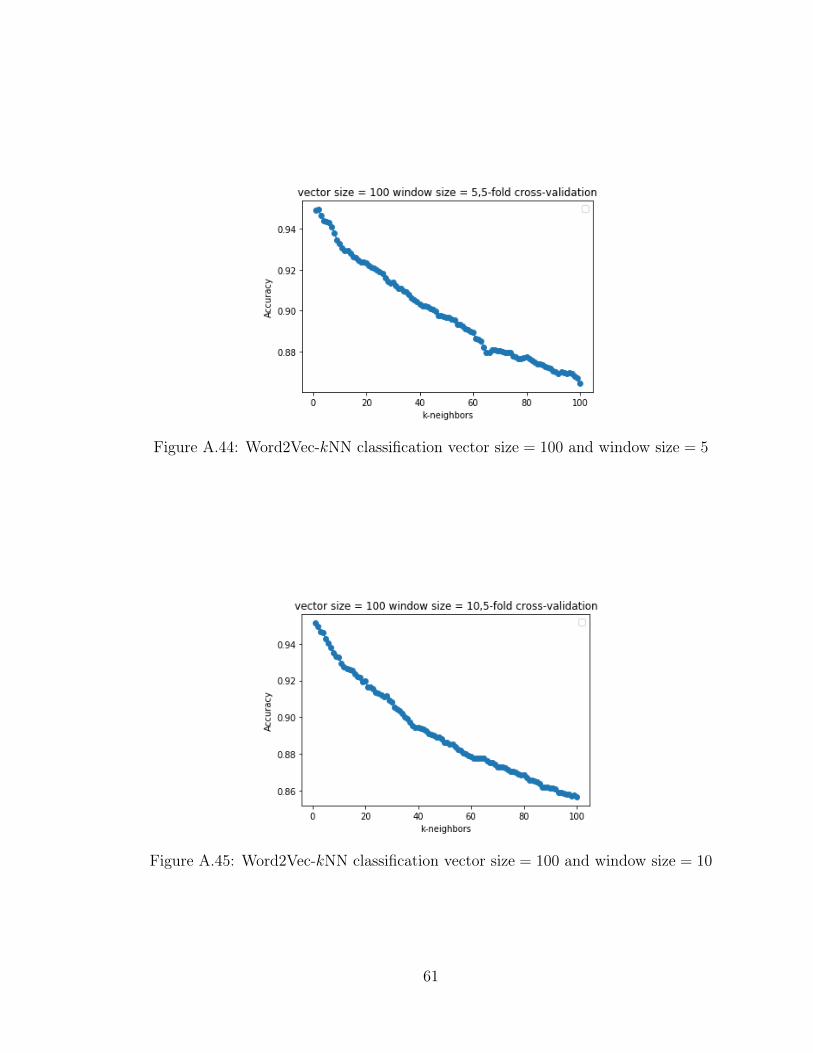
Figure A.44: Word2Vec-𝑘NN classification vector size = 100 and window size = 5
Figure A.45: Word2Vec-𝑘NN classification vector size = 100 and window size = 10
61

Figure A.46: Word2Vec-𝑘NN classification vector size = 100 and window size = 30
Figure A.47: Word2Vec-𝑘NN classification vector size = 100 and window size = 100
62