1

Malnutrition and Inequality in Ecuador

Ana Larrea

Abstract

The objective of this paper is to study whether inequality, independent of poverty and income, is a

determinant of nutritional outcomes among children in Ecuador. Chronic child malnutrition still affects

26% of Ecuadorian children; the prevalence is higher among the indigenous (51%) and in the rural

highlands (47.3%) (LSMS, 2006). We run OLS and two-level multilevel regressions using the -score of

height for age calculated from anthropometric measures in the Living Standards Measurement Survey

(2006), and the Gini coefficient calculated using small area estimates.

In both OLS and ML models we find a significant negative correlation between the -score and the

provincial, county (municipal) and parish (local) Gini coefficients. We also find the squared form of the

Gini coefficient was positive and significant. This implies a negative convex function that flattens out

around a Gini coefficient of 0.51 which we suspect does not invert. In order to incorporate the findings of

Deaton (2003) we control for parishes in which an increase in inequality is coupled with an increase in

average consumption without changing the incidence of poverty. We find it has a significant positive

coefficient in all the OLS models, however, looses significance in most ML models. This suggests the

mean parish -scores are relatively higher; however, we cannot attribute this to the increase in inequality.

Both models control for household consumption and find it has a significant positive coefficient while the

incidence of poverty is not significant. Additionally, we also find that low birth weight and a dummy

variable for indigenous children have a significant negative effect on the -score while that the age and

education of the mother have a significant positive effect.

These results indicate that inequality has a deleterious effect on chronic child malnutrition. We propose

that anxiety and stress which may be associated with inequality is the pathway through which the

correlation between the inequality and chronic child malnutrition is explained. Pre-natal maternal stress

affects intra-uterine growth and is therefore associated with low birth weight, which in turn is a

determinant of chronic malnutrition in children under five (Davey Smith & Egger, 1996; Lynch, et al.,

2000; Lynch, et al., 2001; Lynch, et al., 2004; Wilkinson & Pickett, 2009; Beydoun & Saftlas, 2008;

Camacho, 2008; Mansour and Rees, 2011; Marins & Almeida, 2002; Willey et. al., 2009; Aerts, et al.,

2004; El Taguri, et al., 2009; Adair & David, 1997). These results build on Larrea and Kawachi (2005)

who failed to find a significant correlation at the county or parish levels.

2

1. Introduction

Chronic malnutrition among children is an important public health problem in many Latin American

countries, particularly among indigenous populations in countries with strong socioeconomic disparities

such as Bolivia, Peru and Ecuador (Larrea & Freire, 2002), as well as Guatemala and Honduras (Farrow,

et al., 2005). Its effects are potentially long-term and create deficits in cognition and educational

achievements (Grantham-McGregor, et al., 2000; Walker, et al., 2000). In this sense, it may play an

important role in the intergenerational transmission of poverty. In this paper, we propose inequality,

independent of poverty and income, is a determinant of the nutritional outcomes of ecuadorian children.

Latin America is not the poorest but certainly the most unequal region of the word, which makes it an

ideal testing ground for the association between inequality and malnutrition (Larrea & Kawachi, 2005).

The current perspective on the effect of inequality on health states it is relevant to the extent that a

redistribution of income will allow a less advantaged person to purchase more health than a more

advantaged person with the same amount of income. This argument rests on the concave association

found between individual income and health, which is sufficient to produce and aggregate level

association between income inequality and average health (Rodgers, 1979). However, this perspective

fails to explain, not only how inequality may reflect an underinvestment in health and social infrastructure

(Lynch, et al., 2000) but also fails to explain the psychosocial effects that inequality has on the less

advantaged (Wilkinson & Pickett, 2009).

This study demonstrates there is a significant negative correlation between income inequality and the -

score of height for age – a normalized -score which establishes the growth standard for children under

the age of five (World Health Organization, 2013) – in Ecuador. We find this result for the Gini

coefficient of consumption inequality measured at the provincial, county (municipal) and parish (local)

scale using both OLS and ML models. We also find the squared form of the Gini coefficient is positive

and significant for every geographic level and model. This implies a negative convex function which

flattens out around a Gini coefficient of 0.51. We discuss these results further but suspect the relation

does not invert.

Additionally, we control for parishes where there was an increase in inequality between 2001 and 2010

and where this increase benefited the rich without affecting the relative position of the poor. We find that

this variable is positive and significant in all the OLS models, however, looses significance at the

provincial and county levels in the ML models. The results seem to imply that these parishes have

relatively higher -scores, on average, although we cannot attribute this directly to a change in inequality,

given, firstly, we are not measuring it directly and secondly, the parish driving these results is in

3

Guayaquil, which is the largest city in Ecuador where there is most likely other predictors (see “Other

regressors”).

We control for income by using a per-capita household consumption variable which is positive and

significant and control for poverty by using the head count estimated at the provincial, county and parish

level and find it is not significant in any model. Additionally, we find low birth weight and the dummy

variable for indigenous children is negative and significant, and we show the age and education of the

mother has a positive and significant effect.

An unequal social structure which alienates some people may produce feelings of exclusion, shame and

mistrust among those least advantaged. We find evidence this may translate to an increase in anxiety and

chronic stress (Davey Smith & Egger, 1996; Lynch, et al., 2000; Lynch, et al., 2001; Lynch, et al., 2004).

Chronic amounts of stress makes individuals vulnerable to a wide range of health problems (Wilkinson &

Pickett, 2009), when it presents itself among pregnant women it increases the levels of CHC,1 which

regulates fetal maturation and increases the risk of reduced birth weight (Beydoun & Saftlas, 2008;

Camacho, 2008; Mansour and Rees, 2011). Low birth weight is an important determinant of chronic

child malnutrition (Marins & Almeida, 2002; Willey et. al., 2009; Aerts, et al., 2004; El Taguri, et al.,

2009; Adair & David, 1997). In summary, we propose inequality is associated to low birth weight in

newly born babies through pre-natal stress which predisposes them to chronic child malnutrition.

We process the data in three phases. Firstly, we estimate the Gini coefficient of household per-capita

consumption for every province, county and parish in Ecuador using small area estimates. This

methodology uses the joint distribution of consumption and its covariates estimated on the Living

Standards Measurement Survey of 2006 to generate the distribution of consumption for various

subpopulation of the 2010 census. The resulting consumption estimates allow us to generate the

conditional distribution of the Gini coefficient, its point estimate and its prediction error. Secondly, we

estimate the -score of height for age of children under five years of age using the methodology

developed and distributed freely by the World Health Organization (World Health Organization, 2013)

applied to the anthropometric data available in the Living Standards Measurement Survey (LSMS) of

2006. If a child has a -score under -2, she or he is chronically malnourished. This implies that as the -

score increases nutrition improves. Finally, we estimate multivariable and two-level multilevel

regressions where the natural log of the -score of the height for age is the dependant variable and the

Gini coefficient at various geographic levels are the variables of interest.

1 Croticotrophin-Releasing Hormone

4

This study contributes in that it expands on the evidence first put forward by Larrea and Kawachi (2005)

relating to the same problem in which the authors failed to find a significant correlation between

inequality and the -score at both the county and parish geographic levels. We will firstly review the

literature relating to the effect of inequality on health and malnutrition; secondly, explain the data and

methodology of our estimations; thirdly, present the results of our regression, and, finally, discuss and

conclude our findings.

2. Literary review

Chronic malnutrition, which affects growth and causes stunting (chronic malnutrition) during infancy, has

important deleterious effects on human development. There is considerable evidence that reduced protein-

energy malnutrition is associated with deficits in cognition and school achievements (Grantham-

McGregor, et al., 2000). Grantham-McGregor, et al. (2000) show that there is evidence linking different

kinds of nutritional deficiencies including early childhood protein-energy malnutrition, deficiencies in

iodine, iron, and zinc, short-term food deprivation and inadequate breast feeding to deficits in cognition,

motor performance and behaviour. These effects may be transient or they may last longer and in some

cases may be permanent. In their study Walker et al. (2000) test growth, IQ and cognitive functions of

growth-restricted and non-growth restricted children between the ages of 9 and 24 months, eight years

after the children participated in a 2 year randomized trial of nutritional supplementation and psychosocial

stimulation. The authors find that the group of growth-restricted children has significantly poorer

performance than the group of non-growth-restricted children on a large range of cognitive tests. Their

results support the conclusion that growth restriction has long-term functional consequences (Walker, et

al., 2000).

The literature on the relation between inequality and health indicators focuses on two things, firstly,

functional relationship of these two variables, and secondly, the pathways through which they are

connected. The former is thoroughly reviewed by Wagstaff and Van Doorslaer (2000) who explain the

various theoretical hypotheses as well as the empirical evidence. The latter is explained through a review

of the medical literature on the effect of inequality on stress and pre-natal maternal stress.

i. The functional relation

From Wafstaff and Van Doorslaer’s (2000) research we focus on two main hypotheses: the Absolute

Income Hypothesis (AIH) and the Income Inequality Hypothesis (IIH). The AIH is the notion that

individual health is a concave function of individual income. Therefore, each additional dollar of income

at the individual level raises individual health by progressively smaller amounts. Average health will

improve as average income increases and inequality decreases. Wagstaff and Van Doorslaer (2000) find

5

ample and strong empirical support for the AIH, however, it is important to note that the hypotheses are

not automatically mutually exclusive (Karlsson, et al., 2010). The decreasing tendency of the AIH implies

that there is a threshold beyond which the association between income and health weakens. The

relationship was tested by Lynch at al. (2004) for life expectancy. Among richer countries, the strength of

said association depends crucially on the country and the time period (Lynch, 2000; Lynch, et al., 2000;

Lynch, et al., 2001). The resulting unexplained variation in average health within these richer countries

led to the reasoning that if it is not average income, then perhaps it is the distribution of income within a

country which helps explain the variation in life expectancy (Preston, 1975; Lynch, et al., 2004). The

notion that individual health is a decreasing function of income inequality is known as the IIH. Wilkinson

(1992) demonstrated that the percentage of total post-tax and benefit income obtained by the poorest 70

percent of a country’s population was strongly associated with life expectancy at birth. He showed that

the increases in income inequality in a country were associated with slower increases in life expectancy.

Angus Deaton (2003) explores the existing empirical evidence of a connection between inequality and

health and concludes that there is no direct link to ill health from income inequality per se given there is

no evidence that making the rich richer is hazardous to the health of the poor or their children, provided

that their own incomes are maintained. Notwithstanding, Lynch et al. (2004) presented the a review of 98

studies on inequality and health of which 42% found that all measures of association showed statistically

significant relationships between smaller income difference and better health, another 25% were partially

supportive and 33% provided no support (Wilkinson & Pickett, 2009). Wilkinson & Pickett (2006)

reviewed 168 studies and found that 52% had supportive evidence, 25% had partially supportive evidence

and 22% found no evidence of the association between income inequality and health (Wilkinson &

Pickett, 2009).

Initially, the relationship between inequality and health was seen as an implication of the curvilinear

association between income and health, given that, theoretically, a curvilinear association between

income and health at the individual-level is sufficient to produce and aggregate-level association between

income inequality and health (Rodgers, 1979). However, this implies that redistribution could improve

mean health through the health purchasing power of individual-level income rather than through any

process inherit to inequality. Nevertheless, this perception assumes that inequality influences health

through income rather than social or psychosocial pathways. In the following section we explain the

social and psychosocial pathways which may explain the mechanism through which inequality affects

health in general and malnutrition among children in particular.

ii. The pathways

6

The mechanisms through which inequality affects malnutrition may be complex. The narrative we

propose here is twofold. Firstly, we explore the mechanisms that link income inequality and health

indicators in general through the psychosocial mechanism and secondly, how it affects malnutrition in

particular through pre-natal maternal stress.

a. The general pathways: inequality and health

The general pathway hinges on two separate hypotheses which are interconnected: the neo-material and

the psychosocial, which we explain below. The material conditions relevant to the etiology of infectious

disease in the 19th century are not the same as those relevant to the 20th or the 21st century, given, the

health effects of material conditions are historically contingent and disease specific (Lynch, et al., 2000).

In this sense, income inequality is symptomatic of a lack of resources at the public level. That is to say,

inequality reflects an under-investment in health and social infrastructure given it is the result of a

historical, political and economic process which has influenced the nature and availability of health

supportive infrastructure2. This process shapes the structural matrix of contemporary life which likely

influences individual health, particularly of those who have fewer resources (Lynch, et al., 2000).

Therefore, the scale of material inequality may behave like a skeleton around which other aspects of

status diversification develop (Wilkinson & Pickett, 2009), and, insofar as health indicators depend on the

distribution of social resources, income inequality may actually be a manifestation of the unequal

structural conditions that affect health (Davey Smith & Egger, 1996; Lynch, et al., 2000; Lynch, et al.,

2001; Lynch, et al., 2004). In other words, this lack of resources at the public level may be conducive to

the exclusion of those least advantaged.

More specifically, a social hierarchy in which there are strong perceptions of place and station, common

in relatively unequal societies, is a system which alienates some people and produces negative emotions

among them, such as shame or mistrust. These emotions are translated into antisocial behavior and a

reduction in social capital resulting in a decline in health, either through a psychoneuroendocrine

mechanism or through stress-induced behaviors such as smoking. This hypothesis has been researched in

major review papers (Nguyen & Peschard, 2003) and has been the subject of various international and

governmental organizations reports (Agren, 2003; Bennett, 2003; Health Canada, 1999; Howden-

Chapman & Tobias, 2000; Organization of Economic Cooperation and Development, 2001; Persson, et

al., 2001; Turrell, et al., 1999) which demonstrates a broader acceptance of the hypothesis within the

research and policy community (Lynch, et al., 2004). The recognition of the importance of psychosocial

factors, specifically channeled through chronic stress is a crucial development in our understanding of the

2 Such as the type and quality of education, health services, environmental controls, food availability, housing

conditions, occupational health regulations, etc.

7

social determinants of health. Social environments, particularly low social status, have received greater

attention as a source of chronic stress (Berkman and Glass, 2000; Marmot, 2004; Marmot and Wilkinson,

2005). When we have chronic amount of stress, immunity is down-regulated, there is potential wear on

the cardiovascular system, and we are vulnerable to a wide range of health problems (Wilkinson &

Pickett, 2009).

b. The specific pathways: inequality and chronic child malnutrition

When the psychosocial process manifests itself among pregnant women it has been identified to affect the

birth weight of the child and, in turn, to determine various health and nutritional outcomes of that child

(Beydoun & Saftlas, 2008; Camacho, 2008; Mansour and Rees, 2011).

The medical literature indicates that pre-natal stress increases levels of CHC3, which regulates the

duration of pregnancy and fetal maturation and thus increases the risk of adverse birth outcomes

(Camacho, 2008). Therefore, the effect of stress on intrauterine growth is negative and significant.

Beydoun and Saftlas (2008), in their review of the literature on the effect of pre-natal maternal stress

(PNMS) on fetal growth, find that nine out of 10 studies report significant effects of PNMS on birth

weight, low birth weight (LBW) or fetal growth restriction. However, they also find that the evidence was

predominantly derived from animal studies. Nevertheless, and despite methodological study limitations,

the overall evidence is revealing of an independent association between PNMS and numerous physical

and mental health outcomes (Beydoun & Saftlas, 2008). Almond and Currie (2011) find numerous studies

providing evidence on the long-term consequences of a wide variety of intrauterine shocks (Almond &

Currie, 2011). For example, intrauterine exposure to a terrorist attack or severe famine, even

psychological stress experienced in the first trimester of pregnancy, can reduce birth weight (Camacho,

2008; Eskenazi et al., 2007). Camacho (2008) finds that the intensity of random landmine explosions

during a woman’s first trimester of pregnancy has a significant negative impact on child birth weight.

This finding persists when mother fixed effects are included, suggesting that neither observable nor

unobservable characteristics of the mother are driving the results (Camacho, 2008). Finally, Kaplan et al.

(1996) find that income inequality in the United States was significantly associated with rates of low birth

weight. Insofar as we have argued inequality is associated with stress and pre-natal maternal stress with

LBW, Kaplan et al. (1996) demonstrate the link is measurable and worth researching further.

There are various studies which find that children with LBW are at higher risk to suffer chronic

malnutrition. Marins and Almeida (2002) find in Niterói, Brazil that LBW, low family income, lack of

maternal schooling and lack of potable water connection could be characterized as important under-

3 Croticotrophin-Releasing Hormone

8

nutrition risk factors. They state that the most noticeable among them are the effects of birth weight and

family income, both for the “0-12 months” and for the “above 13 months” age ranges. They argue that, a

child’s birth weight deficits appear to have effects on a child’s growth that extends for years after birth

(Marins & Almeida, 2002). Willey et. al. (2009) found, in Johannesburg and Soweto, that increased

likelihood of stunting (chronic malnutrition) was seen in LBW children, and those who are male (Willey

et. al., 2009). Aerts, et al. (2004) perform a cross-sectional population-based study of determinants of

growth retardation (chronic malnutrition) in under five children in Porto Alegre, Brazil, estimating odd

ratios (OR) for stunting. The main determinants were LBW, per-capita family income, maternal illiteracy

and age, inadequate housing, among others (Aerts, et al., 2004). Taguri et al. (2009), who used a

multivariate analysis in order to ascertain predictors of stunting in children under five in Libya, found that

risk factors were mainly LBW, as well as other variables like paternal education, age, psychosocial

stimulation, source of drinking water and diarrhea (El Taguri, et al., 2009). Adair and David (2007) used a

multivariate discrete time hazard model to estimate the likelihood of becoming stunted in each two month

interval and found that the likelihood of stunting was significantly increased by LBW and other variables

such as diarrhea, febrile respiratory infections and early supplemental feeding. Additionally, they find that

the effect of birth weight was strongest in the first year and that breast-feeding, preventive health care and

taller maternal stature significantly decreased the likelihood of stunting. (Adair & David, 1997). In

addition, birth weight is strongly associated with socioeconomic outcomes later in life (Black, et al. 2007;

Behrman and Rosenzweig, 2004).

These links allow us to formulate a chain of effects that connect high levels of inequality with pre-natal

maternal stress, which in turn has the effect of reducing birth weight, a significant determinant of

malnutrition during infancy. The effects of stress on health through fetal growth are important, not only

because of the increased risk of malnutrition but also because of the long term effects that LBW has on

adult health. Couzin (2002) summarizes how British epidemiologist David Barker of the University of

Southampton established that lower weight babies were likelier to die of coronary heart disease,

hypertension, stroke, and type II diabetes. Roseboom, an epidemiologist at the University of Amsterdam,

found that babies conceived while their mothers suffered from severe malnourishment tended to have the

same problems as their mothers in adulthood. Marelyn Wintour, a fetal physiologist at the University of

Melbourne, Australia, found that the effect of injecting the stress hormone cortisol into pregnant sheep

was that their offspring developed high blood pressure for years. Endocrinologist Hobathan Seckl, of

Western General Hospital in Edinburgh, U.K., believes that excess levels of stress hormones in the fetus

“reset” an important arbitrator of stress in the body, making it hypersensitive to even banal events. In

other words, the body secretes glucose, cortisol, and other stress-related elements when they wouldn’t be

normally needed – a result now observed in LBW humans. Studies in humans and animals suggest that

9

individuals who are under the growth curve and need to catch-up to the rest are in a situation where adult

illnesses linked with LBW is more probable (Couzin, 2002). Currie and Hyson (1999) measure how the

effects of LBW persist well into adulthood and find that the effects are greatest for educational

attainment, followed by self-reported health status and employment (Currie & Hyson, 1999). Behrman

and Rosenzweig (2004) offer estimates which show that intrauterine nutrient intake significantly affects

adult height (Behrman & Rosenzweig, 2004). Almond et al. (2005) found that LBW infants tend to have

lower educational attainment, poorer self-reported health status, and reduced employment and earnings as

adults, relative to their normal weight counterparts (Almond, et al., 2005). If there is a connection

between pre-natal stress and health outcomes in adulthood, then inequality may be an important

determinant of those outcomes in countries where it is high enough to produce high levels of stress among

the most disadvantaged and specifically among disadvantaged women who are pregnant.

This study aims to demonstrate that the effect of inequality on chronic child malnutrition is indeed

significant when measured at various geographic levels by reproducing the ideas put forth by Larrea and

Kawachi (2005) using more recent and higher quality data. The authors examine the association between

economic inequality and child malnutrition in Ecuador. They find economic inequality at the provincial

level, however, not at the county (municipal) or parish (local) level, had a statistically significant

deleterious effect on chronic child malnutrition on both an OLS and a multilevel models (Larrea &

Kawachi, 2005).

The authors propose that the lack of association between income inequality and health in wealthy

countries is due to the threshold effect. This idea, developed by Subramanian and Kawachi (2004), arises

from the fact that studies conducted outside the United States have generally failed to find and association

between income inequality and health. However, almost all the non-US countries listed in these studies

are considerably more egalitarian in their distribution of income than the United States; they have

stronger safety net provisions. Also, when there are cases of relatively more unequal countries there is

some support for the relation (Subramanian & Kawachi, 2004). Therefore, it might be that there is a

threshold beyond which inequality is too low to have a significant effect. This is why we argue that Latin

America is the ideal testing ground for the association between inequality and health given it is the most

unequal region of the world.

3. Data sources and methodology

There are three phases of data processing. The first phase consists of calculating the z-score of height for

age using anthropometric data from the LSMS (2006). Also we calculate the regressors for the model. In

the second phase we calculate per-capita household consumption, the Gini coefficient and the incidence

of poverty for every province, county and parish. This is obtained using small area estimates which

10

combines two data sources: the LSMS (2006) and the Ecuadorian census of 2010. Finally, the third phase

consists of running multivariable and multilevel regressions on the LSMS (2006) where we use the

natural log of the -score of height for age4 as the dependent variable and the estimated Gini coefficient as

the independent variables of interest. In this section we will go over the methodology and results for the

first two phases and in the next section we will cover the results for the regression analysis.

The LSMS of 2006 has national coverage, 55666 observations over 16414 households. Ecuador is divided

into 25 provinces, 224 counties and 1024 parishes; the LSMS covers 22 provinces, 186 counties and 443

parishes. The questionnaire goes over various topics such as living conditions, education, health care,

employment, food consumption and non-food consumption, income, access to credit, migration, and

economic activities such as entrepreneurship and agriculture. This survey includes anthropometric

measures for 5789 children under the age of five (Larrea & Kawachi, 2005). In table 1 we have

descriptive statistics for the variables which are later used in our model. All, except for the Gini

coefficients, are taken directly from the LSMS 2006.

Table 1 Descriptive statistics

Variable Mean Median Min Max Std. Dev. N Weighted Normalized z-score height for age (malnutrition) -1.21 -1.23 -5.53 4.050 1.2138 5789 1364282 Non negative normalized z-score height for age 4.312 4.300 0.000 9.580 1.2138 5789 1364282 Natural Log of non-negative normalized z-score 1.413 1.459 -16.12 2.260 0.3863 5789 1364282 Per-capita household consumption in log form 4.051 4.012 0.750 6.480 0.7339 5772 1361248 Parishes increase inequality 0.164 0.000 0.000 1.000 0.3704 5789 1364282 Provincial Gini coefficient 0.395* 0.401 0.310 0.560 0.0451 5789 1364282 County Gini coefficient 0.388* 0.397 0.290 0.560 0.0444 5789 1364282 Parish Gini coefficient 0.384* 0.388 0.280 0.580 0.0437 5789 1364282 Dummy female 0.484 0.000 0.000 1.000 0.4998 5789 1364282 Mothers years of schooling 8.413 8.000 0.000 22.00 4.1846 5699 1341626 Mothers age 28.37 27.00 12.00 64.00 7.3281 5730 1349604 Dummy indigenous head of household 0.122 0.000 0.000 1.000 0.3276 5789 1364282 Age in months 30.79 31.54 0.070 59.96 17.063 5789 1364282 Housing conditions index 0.5 1.005 -7.33 5.110 1.5075 5569 1286613 Number of children of mother 0.161 0.143 0.000 0.670 0.0809 5637 1328025 Months of exclusive breastfeeding 4.307 5.000 0.000 24.00 2.5964 5424 1284656 Dummy received nutritional supplement 0.245 0.000 0.000 1.000 0.4303 5789 1364282 Dummy rural 0.602 1.000 0.000 1.000 0.4894 5789 1364282 Dummy amazon region 0.064 0.000 0.000 1.000 0.2445 5789 1364282 Dummy rural amazon 0.047 0.000 0.000 1.000 0.2112 5789 1364282 Dummy lack of clean drinking water 0.357 0.000 0.000 1.000 0.4793 5789 1364282 Food consumption index 0 0.105 -3.37 1.480 1.0001 5789 1364282 Dummy low birth weight 0.035 0.000 0.000 1.000 0.1843 5789 1364282

Source: Small Area Estimates using Living Standards Measurement Survey, Ecuadro 2006 (Encuesta de Condiciones de Vida, 2006) and

Ecuadorian Census of 2010. Instituto Nacional de Encuestas y Censos, Ecuador. Data procesing: authors with Unidad de Infromación Socio

Ambiental, Universidad Andina Simón Bolívar.

*It is not possible to take the average of a Gini coefficient given it is not decomposable. This figure is not the Gini coefficient of the country it is here simply to provide the reader an idea of the range of the data.

i. Dependent variable: Child malnutrition measure

We estimate the -score of height for age using the methodology developed and distributed freely by the

World Health Organization (2013). The normalized -score establishes the growth standard of children by

4 We take the natural log of the -score by firstly adding a constant in order to render every value of the -score

positive.

11

defining a normal growth curve (World Health Organization, 2013). We use anthropometric data

available in the LSMS (2006) to calculate the normalized -score for each child below the age of five.

The -score ranges from to as it is measured in standard deviations from the mean which is zero. If

a child’s -score is under -2, that is to say, under two standard deviations below the mean, the child is

chronically malnourished. As such, as it increases the nutritional condition of the child improves. We

calculate the natural log of the -score5 as the dependent variable. Table 2 shows the -score average in

every subregion of the country and Map 1 shows the percentage of children with chronic malnutrition for

every parish (calculated using small area estimates explained below).

Table 2 Summary statistic of z-score of height for age by subregion z-score height for age Mean Median Minimum Maximum Stand. Dev. N N Weighted

Quito -1.248 -1.2 -4.56 2.27 1.04332 319 157670 Guayaquil -0.7587 -0.8 -5.21 2.32 1.09209 454 206543 Urban coast without Guayaquil -1.006 -1.03 -5.11 3.72 1.23375 1171 314686 Rural Coast -1.1849 -1.19 -5.53 4.02 1.13858 1031 252103 Urban highlands without Quito -1.2497 -1.29 -4.62 2.95 1.13763 738 119693 Rural highlands -1.8647 -1.93 -5.51 3.8 1.21635 1494 226448 Urban Amazon -1.1598 -1.13 -3.71 2.03 1.16522 193 23321 Rural Amazon -1.4647 -1.59 -5.25 4.05 1.29647 389 63818 National -1.2176 -1.23 -5.53 4.05 1.21366 5789 1364282

Source: Living Standards Measurement Survey, Ecuadro 2006 (Encuesta de Condiciones de Vida, 2006). Data procesing: authors with Unidad

de Infromación Socio Ambiental, Universidad Andina Simón Bolívar.

Map 1 Incidence of chronic child malnutrition in Ecuador by parish

Source: Small Area Estimates using Living Standards Measurement Survey, Ecuadro 2006 (Encuesta de Condiciones de Vida, 2006) and

Ecuadorian Census of 2010. Instituto Nacional de Encuestas y Censos, Ecuador. Data procesing: authors with Unidad de Infromación Socio

Ambiental, Universidad Andina Simón Bolívar.

ii. Independent variables

5 We take the natural log of the -score by firstly adding a constant in order to render every value of the -score

positive.

12

Our independent variables are measured either at the individual level or at an aggregated geographical

level. The individual variables include what the previous literature on the social determinants of

malnutrition has proven influential (Larrea, Freire, & Lutter, 2001; Larrea, 2002; Marins & Almeida,

2002; Willey et. al., 2009; Aerts, et al., 2004; El Taguri, et al., 2009; Adair & David, 1997). Contextual

variables include per-capita household consumption in log form in order to control for income and the

Gini coefficients along with their quadratic form (Larrea & Kawachi, 2005), as well as, the head count for

poverty both measured at the parish, county and provincial geographic levels. We also try controlling for

intensity and severity of poverty but do not find a significant effect in any model or geographic level and

decided finally not to include them.

a. Small area estimation

The Gini coefficient and the per-capita household consumption are measured at the parish, county and

provincial level using small area estimates. Household surveys that include measures of income and

consumption are rarely representative at the local level or of sufficient size to yield statistically reliable

estimates of poverty or inequality. Similarly, census data, which is generally of sufficient size to allow for

reliability at low levels of aggregation (small geographic scales), usually do not have information about

income or consumption, as is Ecuador’s particular case. Elbers, et al. (2003) use Ecuador as an example

of the method and find that their results have levels of precision comparable to those of survey based

estimates, but for populations as small as 15000 households. The combination of the census data and the

survey data allows for estimations of the Gini coefficient in subpopulations one hundredth the size of the

subpopulations in the survey data and yet obtain very similar prediction errors (Elbers, et al., 2003).

Let be an indicator of poverty or inequality based on the distribution of household-level consumption,

. Using the sample from the Ecuadorian LSMS (2006), a small but rich data sample, we can estimate

the joint distribution of and the covariates . This estimated distribution can be used to generate the

distribution of for any subpopulation of the 2010 census if the set of explanatory variables are

restricted to those which can also be found in this census, in turn allowing us to generate the conditional

distribution of , its point estimate and its prediction error (Elbers, et al., 2003).

Consider equation (1), a linear approximation of the conditional distribution of , where is a sample

cluster and is household, where the vector of disturbances is ( ) To permit for a within cluster

correlation in disturbances we use the equation (2) specification where and are independent of each

other and uncorrelated with (Elbers, et al., 2003).

(1) [ | ]

(2)

13

Basically, an initial estimation of in equation (1) is obtained using OLS and we denote the residuals of

this regression as . With consistent estimates of the residuals can be used to estimate the

variance of (Elbers, et al., 2003).

(3) ( )

Subsequently, we use this estimated distribution (1) to generate the expected value of in a

subpopulation of the census which we denote for village. Thus we write ( ) where is

the -vector of household sizes in village , is the matrix of observable characteristics, and is the

vector of disturbances which is unknown and therefore estimated as we have explained. The expected

value of is then [ | ] where is the vector of model parameters which includes the

disturbances. In constructing an estimator of we replace with . This gives us

[ | ] which is often analytically intractable so simulation is used to obtain the estimator

(Elbers, et al., 2003).

The difference between and the actual level of has three components and can be written as follows

(Elbers, et al., 2003)

(4) ( ) ( ) ( )

The idiosyncratic error – ( ): the difference between the actual value and the expected value of

arises from the unobserved component of consumption and increases as the size of the target population

shrinks which limits the degree of desegregation possible (Elbers, et al., 2003).

The model error – ( ): given are consistent estimators of , is a consistent estimator of and

√ ( ) → ( ) as . However, given that this component of the prediction error is

determined in equation (1), it does not change systematically with changes in the size of the target

population (Elbers, et al., 2003).

The computation error – ( ): when simulation is used as a method of computation, this error has an

asymptotic distribution √ ( ) → ( ) as . Where is the number of independent

random draws used for the simulation and therefore this error can be as small as the computational

resources allow (Elbers, et al., 2003).

Tarozzi & Deaton (2009) argue that, in order to match survey and census data in the way which is

proposed by Elbers et al. (2003), a degree of spatial homogeneity is required for which the method has no

basis and which is unlikely to be satisfied empirically. They argue that, only when at least some aspects of

the conditional distribution of income are the same in the sub-areas within the total area on which the

imputation is calibrated, is there sufficient homogeneity. Given the imputations are projections of

14

expenditure on a subset of whichever variables are available and common between census and survey, the

structural relationships are not necessarily well formed and the coefficients may be the function of local

variables that are relevant and omitted. They use Monte Carlo experiments to show that even a small

amount of heterogeneity may lead to misleading indicators of precision. They argue that estimates based

on those assumptions may underestimate the variance of the error in predicting welfare estimated at the

local level and therefore overstate the coverage of confidence intervals. They demonstrate how area

heterogeneity may appear in an empirical experiment carried out with data from the 2000 Mexican census

(Tarozzi & Deaton, 2009).

In response, Elbers, et al. (2008) perform a similar test in Minas Gerais, Brasil, an area where there is a

strong degree of heterogeneity. They compare their welfare estimates with the true values of the welfare

indicators in a context where the true value is known. They find that, despite concerns regarding area

heterogeneity, and a priori assumptions that the data was unlikely to meet the homogeneity conditions

necessary for the methodology to produce accurate results, the small area estimate approach yielded

estimations of welfare which were quite close to the true values. They also find that the estimations of the

confidence intervals were appropriate. It is important to state that their conclusions hold only after

carefully controlling for community level factors that are correlated with household level welfare (Elbers

et al., 2008). This leads us to believe that even if the method has no bases to check for homogeneity, if the

methodology is applied within relatively homogeneous areas, with careful control over the conditional

distribution of income, the estimations can be reliable.

In this study, as well as in the Elbers et al. (2003) study, Ecuador is divided into eight subregions. Firstly

three general geographic regions: coast, highlands and amazon basin which are divided into rural and

urban areas excluding the two largest cities which are the final two region-cities: Quito and Guayaquil.

Given there can be both rural and urban areas within the same province, county or parish, separating them

increases the level of homogeneity within each sub-region and within each small area estimate model we

run (see appendix for detailed results).

In 2003, Elbers et al. use the LSMS of 1994, and take household per-capita expenditure as their indicator

of wellbeing. They construct populations of increasing sizes from a constant distribution ( ) by

randomly drawing households from the census households in one particular region of the country, the

rural coast. For each population size the table shows the welfare estimations, the standard errors of the

predictions and the share of total variance due to the idiosyncratic component of the error. The

idiosyncratic error is important given that it is the component of the total error which increases with a

reduction in the target population. Elbers, et al. (2003), demonstrate, in table 3, that for a sample of 15000

15

households the idiosyncratic component, , is small and there is little to gain from increasing the sample

size or moving to higher levels of aggregation (Elbers, et al., 2003).

Table 3 Simulation Results

Measure Estimated Values Number of Household

100 1000 15000 100000 Headcount µ 0.46 0.5 0.51 0.51

Total Standard Error 0.067 0.039 0.024 0.024 /Total Variance 0.75 0.24 0.04 0.02

General Entropy (0.5) µ 0.26 0.28 0.28 0.28 Total Standard Error 0.048 0.029 0.022 0.022 / Total Variance 0.79 0.28 0.03 0.01

Source: Redrawn from Elbers, et al., 2003

As they have shown, when combining census and survey data, desaggregating to subregions and

estimating poverty or in our case the Gini coefficient and the per-capita household consumption, for

specific locations becomes possible. When they estimate their welfare indicators by parishes they

demonstrate, in table 4, that one can estimate the Gini coefficient using combined data for subpopulations

one hundredth the size of those one can estimate in survey data and obtain very similar prediction errors

(Elbers, et al., 2003).

Table 4 Improvement using combined data

Region

Sample Data Only (region) Combined Data (suregions)

(2) S.E. of Estimate

(3) Population

(1000s)

(4) S.E. of Estimate

Median

(5) Population

Median (1000s)

Rural Highlands 0.027 2509 0.038 3.3 Rural Cost 0.042 1985 0.046 4.6 Rural Amazon 0.054 298 0.043 1.2 Urban Highland 0.026 1139 0.026 10 Urban Cost 0.03 1895 0.031 11 Urban Amazon 0.05 55 0.027 8 Quito 0.033 1193 0.048 5.8 Guayaquil 0.027 1718 0.039 6.5

Source: Redrawn from Elbers, et al., 2003

In table 5 we present the median standard error, population and number of households in the parishes

within each region of the country. As we can see, the number of households in every parish is well below

the 15000 mark established in Elbers, et al. (2003) which indicates that the total variance due to the

idiosyncratic component of the error might be somewhat above the ideal level (0.24). Nevertheless, the

median standard errors in this study tend to be smaller than those presented by Elbers et al. (2003) and the

population size is similar or larger than those found in Elbers et al. (2003).

16

Table 5 Population size and standard errors of Gini coefficient

Region

Median #households parish (1000s) Median Standard Error (parish) Median Population (parish) (1000s)

This study This study Elbers et al. (2003) This study Elbers et al. (2003)

Quito 4.2 0.0075 0.048 14.4 5.8 Guayaquil 5.3 0.0081 0.039 15.1 6.5 Urban Coast 3.6 0.0102 0.031 9.2 11 Rural Coast 1.1 0.0127 0.046 4.3 4.6 Urban Highlands 2.6 0.0066 0.026 8.2 10 Rural Highlands 0.8 0.0144 0.038 2.8 3.3 Urban Amazon 3.2 0.011 0.027 9.3 8 Rural Amazon 0.4 0.022 0.043 1.4 1.2 National Total 1 0.014

3.6

Source: Redrawn from Elbers, et al., 2003

Table 6 presents the estimations of the Gini coefficient at the regional level obtained using small area

estimates (SAE) and compares them with the Gini coefficient estimated directly from the LSMS (2006).

As can be seen, there is a degree of discrepancy between the LSMS and the SAE point estimations. This

may due to the fact that the models tend to underestimate the household consumption of high income

homes given that the variables we use in our equation (1) estimations are generally measuring lack of

resources. The results of our estimations of small areas can be seen in the following maps.

Table 6 Comparison of estimations of the Gini coefficient from the LSMS (2006) and using SAE (2006-2010)

Region

Regional Gini

LSMS (2006) SAE (2006-2010)

Quito 0.463 0.403 Guayaquil 0.416 0.386 Urban Coast 0.409 0.358 Rural Coast 0.357 0.281 Urban Highlands 0.411 0.346 Rural Highlands 0.454 0.387 Urban Amazon 0.416 0.355 Rural Amazon 0.47 0.454 National Total 0.466 0.419

Source: Small Area Estimates using Living Standards Measurement Survey, Ecuadro 2006 (Encuesta de Condiciones de Vida, 2006) and

Ecuadorian Census of 2010. Instituto Nacional de Encuestas y Censos, Ecuador. Data procesing: authors with Unidad de Infromación Socio

Ambiental, Universidad Andina Simón Bolívar.

Map 2 Mean per-capita household consumption in Ecuador by parish

Source: Small Area Estimates using Living Standards Measurement Survey, Ecuadro 2006 (Encuesta de Condiciones de Vida, 2006) and

17

Ecuadorian Census of 2010. Instituto Nacional de Encuestas y Censos, Ecuador. Data procesing: authors with Unidad de Infromación Socio

Ambiental, Universidad Andina Simón Bolívar.

Map 3 Gini coefficient in Ecuador by parish

Source: Small Area Estimates using Living Standards Measurement Survey, Ecuadro 2006 (Encuesta de Condiciones de Vida, 2006) and

Ecuadorian Census of 2010. Instituto Nacional de Encuestas y Censos, Ecuador. Data procesing: authors with Unidad de Infromación Socio

Ambiental, Universidad Andina Simón Bolívar.

b. Principal component analysis

We use principal component analysis to estimate two indexes. Firstly, we construct a housing conditions

index and secondly a food consumption index. This will allow us to avoid using housing and food

consumption variables which may be highly correlated in our regression model in order to circumvent

high levels of multicollinearity.

The a housing conditions index includes dummy variables for houses with a water connection6, sewage

connection, public garbage collection services, overcrowding, electricity, viable walls7, viable floors

8,

exclusive washroom, and a phone connection (see appendix for detailed results). We found a severe

housing conditions deficiency in the rural highlands and, particularly, in the rural amazon and the rural

coast, where the index has the lowest scores. There is also a considerably low score in Guayaquil (the

largest city in the country), in contradistinction to Quito, the capital.

The main idea of the food consumption index is to use data reduction to identify a small number of

factors that explain most of the variance in the list of 100 food items found in the survey (see appendix for

detailed list). In order to do this, we calculate the amount of calories, carbohydrates, fat and protein for

6 Inside the building 7 Concrete (or similar) 8 Parquet (or similar)

18

every 100 g/ml of every food item. Then, these food items are placed into 9 food groups9 and we calculate

the average calories, carbohydrates, fat and protein consumed for every food group in every parish of the

country (Programa Alimentate Ecuador, Ministerio de Inclusión Económica y Social, Ecuador, 2009).

This results in an index score for each parish which can be compared across parishes.

The model reduced 23 variables to six factors which explain 86.235% of the total variance. The first

factor seems to give high index scores to parishes with high fat and protein consumption. The second

factor seems to give high scores to parishes with high carbohydrate consumption (essentially a potato

based diet, see appendix for details). The parishes which have very low scores on the first factor, and very

high scores on the second factor, indicating high carbohydrate consumption, a severe protein deficiency

and a lack of micronutrient intake from fruits, are essentially those of the rural highlands where we find a

diet composed mainly of carbohydrates from tubers (potatoes) which contrasts strongly to the coastal

region where there is more access to cheap protein staples (fish and seafood). We use the second factor as

our regressor. This variable generally increases in value with the level of carbohydrates consumed on

average (see appendix for detailed results).

c. Other regressors

We include a control variable for parishes in which, as suggested by Deaton (2003), an increase in

inequality is seen to be due exclusively to an increase in the wealth of the rich, which implies inequality

augments without affecting the income of the poor. In order to do this, we estimate the Gini coefficient,

the incidence of poverty as well as the mean consumption for every parish using small area estimates for

both the 2001 census and that of 2010. A parish in which there has been a significant increase in the Gini

coefficient and in consumption coupled with a non-significant change in the incidence of poverty falls

into this category. We find that 7 out of the 443 parishes in the survey fall into this group. They represent

17.3% of the total population and are composed of one parish in Guayaquil (representing 16.2% of the

total population), 4 parishes in the urban amazon and 2 parishes in the rural amazon. Therefore, it seems

safe to say that this coefficient is driven by the effect of Guayaquil (the largest city in the country) in the

sample.

Maternal education as measured by years of schooling, as well as, the age of the mother was included10

.

We estimate an age controlled fertility indicator by which the number of live births a woman has had is

divided by her age since adolescence, as well as, the number of months of exclusive breastfeeding (Larrea

& Kawachi, 2005).

9 Sugars, meats and derivatives, cereals, fruits, fats and oils, eggs and derivatives, milk and derivatives, legumes, fish and seafood, vegetables, tubers, and miscellaneous (containing food items such as salt or coffee). 10 However, we do not include their quadratic form because it rendered both variables insignificant.

19

We attempt to capture basic child health services by the proportion of recommended vaccines11

. However,

this indicator proved to be insignificant so we replaced it with a dummy variable which shows whether

the family received post-partum nutritional supplements from the government12

. We include a dummy

variable for unclean drinking water13

and attempted to include a dummy variable for a diarrhea episode14

in order to control for the effect infectious diseases has on the nutrition of a child, however we chose to

remove it given it is not significant. We also include a dummy variable for rural area (Larrea & Kawachi,

2005).

Fear of discrimination leads some indigenous individuals to feel reluctant to identify as such when asked

directly. This in turn leads to a notorious underestimation of the percentage of indigenous peoples in

Ecuador. In order to avoid this underestimation, we use the fluency of an indigenous language as an

auxiliary variable15

. Specifically, we find an individual to be indigenous if she or he either states it

directly, or if she or he states that the spoken language in the household is an indigenous one (Larrea &

Kawachi, 2005).

4. Results

We ran three OLS models and three two-level multilevel (ML) models, each one with the natural log of

the -score of height for age as the dependent variable and the Gini coefficient calculated at a different

geographical level (provincial, county and parish) as the independent variables of interest. Given the

regressors have different measurement units, standardized beta regression coefficients were estimated to

measure the relative contributions of each variable (Larrea & Kawachi, 2005). The interpretation of the

standardized coefficients is different from traditional coefficients in that they represent a change in the

dependent variable measured in standard deviations as a result of a one standard deviation change in the

independent variable (Fox, 1984).

11 Which include: BCG for tuberculosis, Pentavalente which is DTP for diphtheria, tetanus and pertussis, Hb for hepatitis B and HIB for type b Haemophilus influenzae, poliomyelitis, and finally, measles. 12 Which seems to reflect a selection bias rather than the effects of the treatment, we discuss this further below. 13 For households where members drink water without filtering, boiling or adding chlorine, nor do they buy purified drinking water. 14 In children two weeks prior to the survey 15 Indigenous people are usually fluent in one of various indigenous languages as well as Spanish, whereas it is rare for non-indigenous peoples to be fluent in such languages. Therefore it may be suggested that the fluency in these indigenous languages be used as a proxy for ethnicity.

20

Table 7 Ordinary Least Squares Regression Models OLS 1 OLS 2 OLS 3

b Se b se b se

LN(per-capita consumption) 0.120*** (0.00985) 0.119*** (0.00992) 0.120*** (0.00987) Incidence of poverty - province 0.055 (0.0594) Gini province -0.735*** (1.243) Gini province 2 0.712*** (1.488) Incidence of poverty - county 0.031 (0.0475) Gini county -0.811*** (1.298) Gini county 2 0.794*** (1.589) Incidence of poverty - parish 0.026 (0.0430) Gini parish -0.669*** (1.492) Gini parish 2 0.655*** (1.852) Increased Gini-stable pov. parish 0.057*** (0.0140) 0.055*** (0.0138) 0.053** (0.0139) Dummy female 0.038*** (0.01) 0.038*** (0.01) 0.038*** (0.01) Schooling mother 0.078*** (0.00154) 0.079*** (0.00155) 0.080*** (0.00155) Age mother 0.054*** (0.000683) 0.054*** (0.000681) 0.055*** (0.000682) Dummy indigenous -0.068*** (0.02) -0.069*** (0.02) -0.068*** (0.02) Age months -1.493*** (0.00417) -1.500*** (0.00417) -1.494*** (0.00418) Age months2 2.521*** (0.000143) 2.532*** (0.000143) 2.521*** (0.000143) Age months3 -1.136*** (0.00000144) -1.142*** (0.00000144) -1.135*** (0.00000144) Food consumption index -0.148*** (0.00494) -0.156*** (0.00465) -0.163*** (0.00472) Housing conditions index 0.062* (0.00798) 0.060* (0.00791) 0.057* (0.00786) Number children of mother -0.101*** (0.0727) -0.103*** (0.0728) -0.102*** (0.0724) Number moths breast feeding -0.013 (0.00177) -0.013 (0.00177) -0.014 (0.00176) Dummy gov. nutritional supplement -0.034** (0.01) -0.035** (0.01) -0.036** (0.01) Dummy rural -0.039 (0.02) -0.025 (0.02) -0.018 (0.02) Dummy unclean drinking water -0.032** (0.01) -0.032** (0.01) -0.033** (0.01) Dummy low birth weight -0.159*** (0.04) -0.160*** (0.04) -0.161*** (0.04) _cons 2.538*** (0.27) 2.645*** (0.28) 2.427*** (0.31)

r2 0.221 0.221 0.219 N 5135 5135 5135

Standardized Beta coefficients for numerical variables and unstandardized coefficients for dummy variables and constant. Dependent variable: ln(z-score of height for age)

Table 8 Multilevel Regression Models

MLM1 MLM2 MLM3

b/se Se b/se se b/se se

LN(per-capita consumption) 0.100*** (0.00877) 0.108*** (0.00873) 0.110*** (0.00891) Incidence of poverty - province 0.090 (0.0847)

Gini province -0.759*** (1.415)

Gini province2 0.715*** (1.745)

Incidence of poverty - county

0.064 (0.0808)

Gini county

-0.808*** (1.492)

Gini county2

0.778*** (1.780)

Incidence of poverty - parish

0.029 (0.0620)

Gini parish

-0.675** (1.780) Gini parish2

0.655** (2.160)

Increased Gini-stable pov. parish 0.015 (0.0121) 0.048 (0.0315) 0.058* (0.0223) Dummy female 0.040*** (0.01) 0.041*** (0.01) 0.040*** (0.01) Schooling mother 0.104*** (0.00185) 0.097*** (0.00170) 0.098*** (0.00176) Age mother 0.058*** (0.000689) 0.061*** (0.000664) 0.063*** (0.000673) Dummy indigenous -0.073*** (0.02) -0.086*** (0.02) -0.082*** (0.02) Age months -1.700*** (0.00498) -1.757*** (0.00432) -1.740*** (0.00448) Age months2 2.910*** (0.000164) 3.028*** (0.000138) 2.995*** (0.000145) Age months3 -1.332*** (0.00000159) -1.395*** (0.00000133) -1.382*** (0.00000141) Food consumption index -0.124*** (0.00766) -0.131*** (0.00616) -0.158*** (0.00600) Housing conditions index -0.102*** (0.0533) -0.099*** (0.0700) -0.101*** (0.0693) Number children of mother -0.102*** (0.0533) -0.099*** (0.0700) -0.101*** (0.0693) Months breastfeeding -0.006 (0.00170) -0.007 (0.00169) -0.006 (0.00165) Dummy gov. nutritional supplement -0.032** (0.01) -0.031* (0.01) -0.028** (0.01) Dummy rural -0.047 (0.03) -0.040 (0.03) -0.023 (0.03) Dummy unclean drinking water -0.019 (0.01) -0.021 (0.01) -0.024* (0.01) Dummy low birth weight -0.163*** (0.02) -0.165*** (0.02) -0.162*** (0.02) _CONS 2.624*** (0.29) 2.680*** (0.31) 2.477*** (0.37)

Random slope (Gini province) 0.118 (0.589)

Random slope (Gini county)

0.000000865 (0.0000218)

Random slope (Gini parish)

0.0000101 (0.000119) Random intercept (constant) 0.0000209 (0.00549) 0.0746 (0.0216) 0.0907 (0.0169) Total standard deviation (Residual) 0.292 (0.116) 0.288 (0.0127) 0.283 (0.0115)

N 5135 5135 5135

Standardized Beta coefficients for numerical variables and unstandardized coefficients for dummy variables and constant. Dependent variable: ln(z-score of height for age)

21

Discussion

In both the OLS models and the ML models the effect of consumption on the natural log of the -score is

positive and significant. We find both in the OLS and the ML models that the incidence of poverty

measured at the provincial, county and parish level is not significant.

i. The effect of inequality

In both the OLS and the ML models the Gini coefficient is negative and significant and its quadratic form

is positive and significant at every geographic level.16

These results show a correlation which suggests

that the distribution of income is as important a determining factor as income, however, as it increases its

effect flattens out in a negative convex function.

By taking the partial derivative of the -score17

with respect to the Gini coefficient we can establish the

minimum point of the negative convex function created here. In the OLS models we find the minimum

point at a Gini coefficient of 0.52 at the provincial level, 0.51 at the county level and 0.51 at the parish

level. In the ML models we find minimum points at a Gini coefficient of 0.53 at the provincial level, 0.52

at the county level and 0.52 at the parish level. These results imply that beyond the minimum point, at

very high levels of inequality, the relationship between malnutrition and inequality may invert. However,

this is unlikely given the maximum Gini coefficient in our data is 0.5598, 0.564 and 0.5751 at the

provincial, country and parish level respectively. Although, this phenomenon may be interesting to

investigate further.

Larrea and Kawachi (2006) do no find a significant relationship between consumption inequality and

chronic child malnutrition at the county or at the parish level, in spite of using multilevel models in

addition to multivariable regressions. This may be due to the lack of quality data with information on

child nutrition, as well as the smaller sample size. The LSMS of 1998 has a sample of 2723 children

under the age of five which is a little over half of the sample (5789) we have available in the LSMS 2006

survey (Larrea & Kawachi, 2005).

Finally, we control for parishes where, as suggested by Deaton (2003), we found a significant increase in

inequality due exclusively to an increase in the wealth of the rich without affecting the income of the

poor. This dummy variable is positive and significant in every OLS model; however, in the ML models

this variable looses significance at the provincial and county levels and is positive and significant only in

the third model where the Gini coefficient is measured at the parish level. These results indicate that these

parishes have relatively higher -scores, on average. However, we cannot say that it is the increase in

16 The Gini coefficient is calculated at the parish, county and provincial scale. 17 In natural log form

22

inequality which caused this reduction given that we are not correlating the change in inequality in these

parishes directly with the -score. Also, the parish driving these results is in Guayaquil, which is the

largest city in Ecuador where there is likely other predictors (see “Other regressors”).

ii. Other effects

We find that the dummy variable for low birth weight is negative and significant in all the OLS and ML

models. This gives us an indication that a child born with low weight is prone to malnutrition during

infancy, as stated in the literary review. The variable measuring the age of the child in months is negative

and significant in all the OLS and ML models, indicating that as the child grows (and perhaps is no longer

breastfeeding) chronic malnutrition sets in. Also, we find that the dummy variable for female children is

positive and significant in every OLS and ML model demonstrating that boys suffer from lower -scores,

on average, than girls.

Both the schooling and the age of the mother are positive and significant and our fertility variable18

is

negative and significant in every OLS and ML model indicating that the -score is higher, on average,

among children with relatively older more educated mothers, and lower, on average, among those with

relatively younger mothers who have relatively more children.

The coefficient for the dummy variable denoting indigenous children is negative and significant, showing

that this group, on average, has relatively lower z-scores. This is demonstrated in the high prevalence of

malnutrition among indigenous children (51%) which is twice as high as among non-indigenous children

(26%) (LSMS, 2006).

The housing condition index which increasing with living conditions is positive and significant in every

OLS and ML model. The unclean drinking water regressor is negative and significant in every OLS

model but looses significance at the provincial and county level in the ML model. The food consumption

index, which increases in households where there is a high consumption of carbohydrates as opposed to

protein, vitamins and minerals, is negative and significant in every OLS and ML model.

The number of months of breastfeeding is not significant in either the OLS models or the ML models.

Government supplied nutritional supplements is significant but negative in all the OLS and ML models.

These supplements refer to a dehydrated powder containing supplemental nutrients intended to be mixed

with water and fed to the children of the household in order to prevent chronic malnutrition. The sample

of people who receive this government aid is obviously not random given they distribute it among those

who need it the most. Therefore, the results of this regressor have a systematic error, given that some

members of the population in our survey data are less likely to be included than others, creating a

18 This variable is the number of live birth a woman has had divided by her age since adolescence.

23

selection bias. This does not allow us to distinguish between the effects of the treatment and the effects of

the bias in the sample.

5. Conclusion

This study demonstrates the relevance of inequality as a determinant of chronic child malnutrition by

expanding on the ideas first put forward by Larrea and Kawachi (2005). We show that the correlation

between inequality and the -score of height for age is significant and negative at the province, county

and parish level and that its quadratic form has a significant positive coefficient in both OLS and ML

models. Therefore, we find a nonlinear negative effect in which malnutrition is affected in decreasing

amounts by the Gini coefficient, flattening out as it reaches a minimum point around a Gini coefficient of

0.51. We also find that income is positive and significant and that the incidence of poverty, measured at

the province, county and parish scale is not significant in every model.

Additionally, we use a control variable for the parishes in which there was an increase in inequality

between 2001 and 2010 coupled with an increase in average consumption without affecting the incidence

of poverty. We find that this variable is positive and significant in all the OLS models. However, looses

significance at the provincial and county levels in the ML models. This indicates that the -score is

relatively higher, on average, in these parishes. However, we cannot attribute this effect to a change in

inequality given, firstly, we are not measuring it directly, and secondly, the parish driving these results is

in Guayaquil, which is the largest city in Ecuador where there is most likely other predictors (see “Other

regressors”).

Finally, we find that low birth weight and the dummy variable for indigenous have a significant negative

effect on the -score; and also, that the mothers age and education have a positive and significant effect

on the -score, which coincides with the findings of Larrea and Kawachi (2005).

It is our contention that an unequal income distribution behaves like a frame around which other aspects

of status diversification develop. This frame shapes the structural matrix of living conditions which

influence individual health. More specifically, an unequal social structure which alienates some people

may produce feelings of exclusion, shame and mistrust among those lest advantaged and this may

translate into a reduction in social capital and an increase in anxiety and chronic stress (Davey Smith &

Egger, 1996; Lynch, et al., 2000; Lynch, et al., 2001; Lynch, et al., 2004). Chronic amounts of stress is

associated with a down-regulated immune system and a potential wear on the cardiovascular system

which makes individuals vulnerable to a wide range of health problems (Wilkinson & Pickett, 2009).

Chronic stress among pregnant women increases levels of CHC,19

which regulates fetal maturation and

19 Croticotrophin-Releasing Hormone

24

increases the risk of reduced birth weight (Beydoun & Saftlas, 2008; Camacho, 2008; Mansour and Rees,

2011). Low birth weight is one of the most important determinants of chronic child malnutrition (Marins

& Almeida, 2002; Willey et. al., 2009; Aerts, et al., 2004; El Taguri, et al., 2009; Adair & David, 1997).

We propose this pathway as an explanation of the relevance of inequality which is alternative to the view

that it has no inherit influence, rather, it is simply the consequence of the curvilinear association between

income and health.

Bibliography

Adair, L. S., & David, K. G. (1997). Age-Specific Determinants of Stunting in Filipino Children. The

Journal of Nutrition, 127, 314-320.

Aerts, D., Drachler, M., & Justo Giugliani, E. R. (2004). Determinants of Growth Retardation in Southern

Brazil. Cadernos de Saúde Pública, 20(2), 1182-1190.

Agren, G. (2003). Sweden´s new public health policy. Stockholm: Swedish National Institute of Public

Health.

Almond, D., Chay, K. Y., & Lee, D. S. (2005). The Costs of Low Birth Weight. The Quarterly Journal of

Economics, 120(3), 1031-1082.

Behrman, J. R., & Rosenzweig, M. R. (2004). Returns to Birthweight. The Review of Economics and

Statistics, 86(2), 586-601.

Bennett, J. (2003). Investment in population health in five OECD countries. Paris: OECD Health Working

Paper no. 2.

Berkman, L., Glass T. (2000). Social integration, social networks, social support, and health. In Social

Epidemiology, ed. L. Berkman and I. Kawachi, 137-177. New York: Oxford University Press.

Beydoun, H., & Saftlas, A. (2008). Phiysical and mental health outcomes of prenatal maternal stress in

human and animal studies, a review of recent evidence. Pediatic and Perinatal Epidemiology,

22(5), 438-466.

Black, S. E., Devereux, P. J., & Salvanes, K. G. (2007). From the cradle to the labor market? The effect of

birth weight on adult outcomes. The Quarterly Journal of Economics, 122(1), 409-439.

Blakely, T. A., Lochner, K., & Kawachi, I. (2002). Metropolitan area income inequality and self-related

health. Social Science & Medicine, Vol. 51, 1343-1350.

Camacho, A. (2008). Stress and birth weight: evidence from terrorist attacks. American Economic

Review, 98(2), 511-515.

25

CEPAL. (2011). CEPALSTAT. Retrieved 06 06, 2013, from

http://websie.eclac.cl/sisgen/ConsultaIntegrada.asp

Couzin, J. (2002). Quirks of fetal environment felt decades later. Science, 296, 2167-2169.

Currie, J., & Hyson, R. (1999). Is the Impact of Health Shocks Cushioned by Socioeconomic Status? The

Case of Low Birthweight. The American Economic Review, 89(2), 245-250.

Davey Smith, G., & Egger, M. (1996). Commentary: Understanding it all - Health, meta-theories, and

mortality trends. British Medical Journal, 313(7072), 1584-1585.

Deaton, A. (2003). Health, Inequality, and Economic Development. Journal of Economic Literature, XLI,

113-158.

El Taguri, A., Betilmal, I., Mahmud, S. M., Monem Ahmed, A., Goulet, O., Galan, P., & Hercberg, S.

(2009). Risk factors for stunting among under-fives in Libya. Public Health Nutrition, 12(8),

1141-1149

Elbers, C., Lanjouw, J. O., & Lanjouw, P. (2003). Micro-Level Estimation of Poverty and Inequality.

Econometrica, 71(1), 355-364.

Elbers, C., Lanjouw, P., & Leite, P. G. (2008). Brazil within Brazil: Testing the poverty map

methodology in Minas Gerais.

Eskenazi, Brenda; Marks, Amy R.; Catalano, Ralph; Bruckner, Tim; Toniolo, Paolo G. (2007) Low

birthweight in New York city and upstate New York following the events of September 11th.

Human Reproduction, 22(11), 3013-3020.

Farrow, A., Larrea, C., Hyman, G., & Lema, G. (2005). Exploring the spatial variation of food poverty in

Ecuador. Food Policy, 30, 510-531.

Fox, J. (1984). Linear statistical models and related methods: With applications to social research. New

York: Wiley.

Freire, Wilma B., Silva, Katherine M., Ramírez, María J., Waters, William F., and Larrea. Ana P. (2014).

The double burden of under nutrition and excess body weight in Ecuador. Submitted to the

American Journal of Clinical Nutrition.

Grantham-McGregor, S. M., Walker, S. P., & Chang, S. (2000). Nutritional deficiencies and later

behavioural development. Proceedings of the Nutrition Society, 59, 47-54.

Health Canada. (1999). Toward a healthy future: Second report on health of Canadians. Ottawa: Minister

of Public Works and Government Services Canada.

26

Howden-Chapman, P., & Tobias, M. (2000). Social inequalities in health: New Zealand 1999.

Wellington: Ministry of Health.

Kaplan G.A., Pamuk, E.R., Lynch, J.W., Cohen, R.D., Balfour, J.L. (1996). Inequality in income and

mortality in the United States: analysis of mortality and potential pathways. BMJ, 312, 199-

1003.

Karlsson, M., Nilsson, T., Lyttkens, C. H., & Leeson, G. (2010). Income inequality and health:

Importance of a cross-country perspective. Social Science & Medicine, 70, 875 - 885.

Larrea, C. (2002). Social inequality and child malnutrition in eight Latin American countries.

Unpublished paper, Harvard Center for Society and Health.

Larrea, C., & Freire, W. (2002). Social inequality and child malnutrition in four Andean countries. Pan

American Journal of Public Health, Vol. 11 (5/6), 356-364.

Larrea, C., & Kawachi, I. (2005). Does economic inequality affect child malnutrition? The case of

Ecuador. Social Science and Medicine, 60, 165-178.

Larrea, C., & Montenegro Torres, F. (2006). Ecuador. In G. Hall, & H. A. Patrinos, Indigenous peoples,

poverty and human development in Latin America 1994-2004 (pp.67-105). New York: Palgrave

MacMillan.

Larrea, C., Freire, W., & Lutter, C. (2001). Equidad desde el principio: Situación nutricional de los niños

ecuatorianos. Washington, DC: Organización Panamericana de la Salud.

Lynch, J. (2000). Income Inequality and Health: Expanding the Debate. Social Science and Medicine,

51(7), 1001-1005.

Lynch, J., Davey Smith, G., Harper, S., Hillemeier, M., Ross, N., Kaplan, G. A., y otros. (2004). Is

income inequality a determinant of population health? Part 1. A systematic review. The Milbank

Quarterly, 82(1), 5-99.

Lynch, J., Davey Smith, G., Hillemeier, M., Shaw, M., Raghunthan, T., & Kaplan, G. (2001). Income

inequality, the psychosocial environment, and health: Comparisons of wealthy nations. Lancet,

358, 194-200.

Lynch, J., Due, P., Muntaner, C., & Davey Smith, G. (2000). Social capital - Is it a good investment

strategy for public health? Journal of Epidemiology and Community Health, 54(6), 404-408.

27

Lynch, J., Kapaln, G., Davey Smith, G., & House, J. (2000). Income inequality and mortality: Importance

to health of individual income, psychosocial environment, or material conditions. British

Medical Journal, 320(7243), 1200-1204.

Mansour, H., & Rees, D. (2011). The effect of prenatal stress on birth weight: Evidence from the al-Aqsa

Intifada. IZA Discussion Paper No 5535.

Marins, V., & Almeida, M. (2002). Undernutrition prevalence and social determinants in children aged 0-

59 months, Niterói, Brazil. Annals of Human Biology, 29(6), 609-618.

Marmot, M. (2004). Status Syndrome: How Your Social Sanding Directly Affects Your Health and Life

Expectancy. London: Bloomsbury.

Marmot, M. & Wilkinson, R. (2006). Social Determinans of Health. Oxford: Oxford University Press.

Nguyen, V.-K., & Peschard, K. (2003). Anthropology, inequality and disease: A review. Annual Review

of Anthropology, 32, 447-474.

Organization of Economic Cooperation and Development. (2001). The well-being of nations: The role of

human and social capital. Paris: OECD, Centre for Educational Redearch and Innovation.

Persson, G., Bostrom, G., Diderichsen, F., Lindberg, G., Pettersson, B., Rosen, M., Stenbeck, M., Wall, S.

(2001). Health in Sweden. The national public health report, 2001. Scandinavian Journal of

Public Health, 29(58), 199-218.

Preston, S. (1975). The changing relation between morality and level of economic development.

Population Studies, 29, 231-248.

Programa Alimentate Ecuador, Ministerio de Inclusión Económica y Social, Ecuador. (2009). Lista de

alimentos de la Encuesta de Condiciones de Vida. Quito: Unpublished.

Rodgers, G. (1979). Income and inequality as determinants of mortality: An international cross-section

analysis. Population Studies, 33, 343-351.

Steckel, R. H. (1995). Stature and the standard of living. Journal of Economic Literature, 33(4), 1903-

1940.

Subramanian, S. V., & Kawachi, I. (2004). Income Inequality and Health: What Have We Learned So

Far? Epidemiologic Reviews, 26, 78–91.

Tarozzi, A., & Deaton, A. (2009). Using Census and Servey Data to Estimate Poverty and Inequality for

Small Areas. The Review of Economics and Statistics, 91(4), 733-792.

28

Turrell, G., Oldenburg, B., McHuffog, I., & Dent, R. (1999). Socioeconomic determinants of health:

Towards a national research program and a policy and interventional agenda. Canberra:

Queensland University of Technology, School of Public Health, Ausinfo.

Wafstaff, A., & Van Doorslaer, E. (2000). Relative income, race and mortality. Annual Revision Public

Health, 21, 543–567.

Walker, S. P., Grantham-McGregor, S. M., Powel, C. A., & Chang, S. M. (2000). Effects of growth

restriction in early childhood on growth, IQ, and cognition at age 11 to 12 years and the benefits

of nutritional supplementation and psychosocial stimulation. The Journal of Pediatrics, 137(1),

36-41.

Wilkinson, R. (1992). Income distribution of life expectancy. British Medical Journal, 304(6820), 165-

168.

Wilkinson, R. G., & Pickett, K. E. (2006). Income inequality and population health: a review and

explanation of the evidence. Social Science and Medicine, 62, 1768-1784.

Wilkinson, R. G., & Pickett, K. E. (2009). Income inequality and social dysfunction. Annual Review of

Sociology, 35, 493-511.

Willey, B. A., Cameron, N., Norris, S. A., Pettifor, J. M., & Griffiths, P. L. (2009). Socio-economic

predictors of stunting in preschool children: a population-based study from Johannesburg and

Soweto. SAMJ: South African Medical Journal, 99(6), 450-456.

World Health Organization. (2013). WHO Child Growth Standards: Methods and development. Retrieved

from http://www.who.int/childgrowth/publications/technical_report_velocity/en/index.html

World Health Organization. (2013). World Health Organization, Child Growth Standards. Retrieved from

http://www.who.int/childgrowth/software/en/

29

Appendix 1: Equation (1) for Small Area Estimates

We construct a separate model for each subregion Dependent Variable: LNCONPCM Weighted by: FEXP Quito Guayaquil Urban Coast Rural Coast Urban Highlands Rural Highlands Urban Amazon Rural Amazon

_intercept_ 3.9244*** 4.69609*** 4.95897*** 4.24822*** 4.66441*** 3.81323*** 4.21719*** 5.12909***

(0.54644) (0.32232) (0.17108) (0.16086) (0.23849) (0.17533) (0.33065) (0.2845)

Access to higher education 0.90309***

(0.09756)

Average proportion of household with cement walls in statistical area

-0.14443***

0.13408***

(0.04016)

(0.03017)

Average proportion of houses with connection to public water disposal service

-0.16132** -0.12525**

(0.05754) (0.03788)

Average proportion of housing with exclusive toilets in statistical area -0.11827

-0.11533

0.22179**

(0.14344)

(0.06497)

(0.07307)

Average proportion of houses with garbage truck service in statistical area 1.231*

-0.12598*

(0.5303)

(0.05113)

Average proportion of houses with publicly provided drinking water in statistical area

0.05851

-0.32875**

(0.03787)

(0.11025)

Average proportion of persons per room in statistical area

-0.20641 -0.05895**

-0.06983*** 0.04303 -0.20006***

(0.15818) (0.02121)

(0.01585) (0.02425) (0.02644)

Average years of schooling in parish

0.04799**

(0.0176)

Dummy amplified nuclear family

-0.08971** 0.05536*

(0.02868) (0.02572)

Dummy Cuenca

0.16585***

(0.02294)

Dummy bamboo flooring or similar

-0.21931** -0.07458 -0.09438**

-0.06947**

(0.07354) (0.0439) (0.03403)

(0.02424)

Dummy for cement or brick flooring

-0.1966***

-0.08137***

(0.04597)

(0.02228)

Dummy for walls made of bamboo wood or similar

-0.17853** -0.06676*

(0.0547) (0.0309)

Dummy head of household affiliated to social security

0.08396** 0.0631** 0.11415**

0.1265***

(0.03172) (0.0237) (0.03546)

(0.03291)

Dummy head of household construction worker

-0.0573 0.32542*** -0.12684* 0.08557*** 0.12598*** 0.20716***

(0.04312) (0.06257) (0.04962) (0.02146) (0.02989) (0.05118)

Dummy head of household directive position 0.17944* 0.31372***

0.27233*

0.31744**

(0.07427) (0.067)

(0.12508)

(0.10396)

Dummy head of household employer 0.09348 0.15455*** 0.23413*** 0.19037*** 0.22634*** 0.16207*** 0.21176**

(0.05634) (0.04382) (0.02869) (0.02919) (0.03255) (0.03692) (0.06899)

Dummy head of household ethnic 0.07023 0.07685

-0.14128**

(0.05121) (0.04629)

(0.04509)

Dummy head of household female -0.08383*

-0.09081** 0.04279

(0.03465)

(0.02807) (0.02744)

Dummy head of household in hotel industry

0.12719* 0.12641

(0.04931) (0.07932)

Dummy head of household in manufacturing

0.05821

(0.03067)

Dummy head of household in retail sale

0.10744*** 0.04692 0.0947**

-0.0909 -0.39423***

(0.02441) (0.03929) (0.02895)

(0.06048) (0.10429)

Dummy head of household inactive

0.09164*

0.04816

0.4985***

(0.04158)

(0.03294)

(0.1199)

Dummy head of household marital status divorced/separated

-0.05765* 0.00655

(0.02748) (0.03115)

Dummy head of household marital status single

-0.13252*** -0.06892

-0.11749***

(0.03986) (0.04049)

(0.03471)

Dummy head of household non-qualified agricultural worker

0.0731*

-0.23459***

(0.0363)

(0.053)

Dummy head of household non-qualified worker

-0.04806*

(0.02252)

Dummy head of household other service position -0.15888 0.12451*

-0.11051

(0.08409) (0.05073)

(0.06869)

Dummy head of household over 65 years of age

-0.15334** -0.07733* -0.158***

(0.04989) (0.03123) (0.02902)

Dummy head of household public sector

0.38836 0.15076***

0.2044 -0.36949* 0.23886**

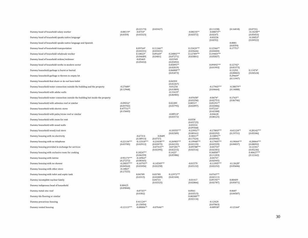
30

(0.22173) (0.03427)

(0.11238) (0.16818) (0.0731)

Dummy head of household salary worker -0.08119* -0.0754*

-0.08235** -0.08073**

-0.14238**

(0.0359) (0.03323)

(0.02572) (0.0247)

(0.05453)

Dummy head of household speaks native language

-0.03236

-0.10053*

(0.0292)

(0.04922)

Dummy head of household speaks native language and Spanish

0.0881

(0.0559)

Dummy head of household transportation

0.09764* 0.11166**

0.15424*** 0.12366** 0.17751*

(0.04331) (0.03431)

(0.03626) (0.04404)

Dummy head of household wholesale worker

0.10023* 0.09169* 0.24802*** 0.12789*** 0.19403***

(0.04689) (0.0401) (0.07271) (0.03801) (0.05837)

Dummy head of household widow/widower

-0.05469

-0.01949

(0.05432)

(0.03492)

Dummy head of household works in modern sector

0.05895**

0.09492*** 0.12742*

(0.02019)

(0.01993) (0.05373)

Dummy household garbage is burnt or buried

0.06808***

0.13293 0.11474*

(0.01873)

(0.08065) (0.04524)

Dummy household garbage is thrown in empty lot

0.29669*

(0.11947)

Dummy household that share or do not have toilet

0.04359

(0.02267)

Dummy household water connection outside the building and the property -0.27689*

-0.01256

-0.17965*** -0.38079**

(0.12968)

(0.01809)

(0.04664) (0.14088)

Dummy household with adobe walls

-0.15419*

(0.06985)

Dummy household water connection outside the building but inside the property

-0.07658* -0.0674* 0.1763**

(0.03296) (0.02751) (0.06746)

Dummy household with asbestos roof or similar -0.09016*

0.02289 0.00517 0.05291**

(0.03702)

(0.03795) (0.02097) (0.02006)

Dummy household with electric stove 0.47731**

0.97216*

(0.15683)

(0.42308)

Dummy household with palm/straw roof or similar

-0.08914*

-0.04628

(0.03572)

(0.08125)

Dummy household with room for rent

0.0358

(0.03725)

Dummy household with wood walls

-0.05554

(0.09368)

Dummy household wood/coal stove

-0.10355*** -0.23951** -0.17803*** -0.61124** -0.28142***

(0.02589) (0.08161) (0.02292) (0.19751) (0.05506)

Dummy housing with no electricity

-0.67314 0.0689

-0.38417* -0.10891**

(0.38913) (0.0757)

(0.17524) (0.03945)

Dummy housing with no telephone -0.22134*** -0.13318*** -0.23438*** -0.26983*** -0.19948*** -0.17905*** -0.19044*** -0.28064***

(0.03785) (0.02912) (0.02075) (0.04135) (0.02135) (0.02539) (0.04837) (0.08092)

Dummy housing provided in exchange for services

-0.07415** -0.07281** -0.09788*** -0.04755*

-0.12341*

(0.02395) (0.02215) (0.02516) (0.02301)

(0.05236)

Dummy housing with exclusive room for cooking

0.18247**

0.1422*

0.36858**

0.40627***

(0.06259)

(0.05986)

(0.11203)

(0.12162)

Dummy housing with latrine -0.95173*** -0.18963*

-0.04757

(0.27272) (0.08365)

(0.02945)

Dummy housing with no shower -0.20037*** -0.10793** -0.14549***

-0.01579 -0.11995*** -0.13628*

(0.04564) (0.03456) (0.02258)

(0.03132) (0.02232) (0.05606)

Dummy housing with other stove -0.14827

(0.17555)

Dummy housing with toilet and septic tank

0.04789 0.03785 0.12972***

0.0763***

(0.0315) (0.02089) (0.02104)

(0.02111)

Dummy incomplete nuclear family

0.04721

-0.01417 0.09195** 0.08409

(0.02525)

(0.02866) (0.02787) (0.05071)

Dummy indigenous head of household 0.08425

(0.09848)

Dummy metal zinc roof

-0.07327*

0.0561

0.0607

(0.0302)

(0.03515)

(0.04587)

Dummy tile flooring or similar

0.08308***

(0.02116)

Dummy precarious housing

0.41124**

-0.12429

(0.15054)

(0.07863)

Dummy rented housing -0.12113*** -0.08006** -0.07646**

-0.08938* -0.12164*

31

(0.03102) (0.0302) (0.02409)

(0.04269) (0.04872)

Dummy semi-precarious housing

0.13243** 0.08558* 0.04575

-0.12763***

(0.04624) (0.0334) (0.03728)

(0.03208)

Dummy tile flooring or similar

0.05854 0.19685*** 0.23252***

0.11607* 0.14214**

(0.05148) (0.02308) (0.04915)

(0.04679) (0.05326)

Elementary school attendance net rate

0.23752 -0.54376**

(0.16138) (0.18509)

Head of household education * dummy head of household formal sector 0.0108**

0.01024***

(0.00329)

(0.00183)

Head of household education * dummy head of household public sector

0.00409 0.00498*

-0.02533*

(0.00289) (0.00227)

(0.01004)

Head of household education * dummy head of household house worker

-0.02849**

-0.07134*

(0.00974)

(0.03342)

Head of household education * dummy head of household public sector

-0.02311

0.01864

(0.0149)

(0.01284)

Head of household education * head of household experience 0.00017 0.00078*** 0.00027** 0.00065*** 0.00046***

(0.00024) (0.00022) (0.0001) (0.00012) (0.000074955)

Head of household experience 0.00323

-0.00072 0.01974*

0.0009

(0.00436)

(0.00214) (0.00993)

(0.00104)

Head of household experience2 0 -0.00036*

-0.00093*

(0) (0.00014)

(0.00036)

Head of household experience3

0* 0 0.000011198**

(0)

(0)

Head of household schooling 0.01307 -0.03468*

0.03081*** 0.00616

0.02007***

(0.01875) (0.01688)

(0.00305) (0.00684)

(0.00584)

Head of household schooling2 0.00066 0.0012 0.00081*** 0.0004

0.00168*** 0.00078*

(0.00068) (0.00064) (0.0002) (0.00027)

(0.00043) (0.00033)

High school attendance net rate in parish 0.15497* -0.05731 0.05553 0.09346**

-0.07176*

(0.06223) (0.0506) (0.04261) (0.03176)

(0.03481)

Household water obtained from stream or similar

-0.13784***

0.09818** 0.17614

(0.03786)

(0.03553) (0.10576)

Household water obtained well

-0.13309*** 0.03924*

0.18506**

(0.03445) (0.01996)

(0.064)

Household with room for family business

0.03804

0.2489***

(0.03129)

(0.07349)

Household with toilet without septic tank, just dung up well

-0.02735

-0.1627*

0.09123

(0.07835)

(0.05648)

Ln(Income per-capita) 0.04942*** 0.17483***

0.14104***

0.14508*** 0.11786*** 0.17597***

(0.01444) (0.02635)

(0.01217)

(0.01589) (0.0289) (0.03269)

Percentages of houses in parish with parquet floors or similar

-0.39243

0.08402 -0.26581

(0.24413)

(0.07599) (0.20628)

Rate of literacy in statistical area

0.37477*

0.40517 0.21459**

(0.14607)

(0.2192) (0.07405)

Rooms per person 0.22059*** 0.25524*** 0.21138*** 0.16251*** 0.21087*** 0.18977*** 0.14312** 0.09979**

(0.02652) (0.03094) (0.01879) (0.01775) (0.01513) (0.01748) (0.04331) (0.03445)

Square root of number of basic needs met -0.08573*** -0.06066 -0.05829** -0.13819*** -0.11805*** -0.08635** -0.21112*** -0.1249***

(0.02511) (0.03152) (0.01799) (0.0273) (0.02079) (0.02689) (0.04291) (0.03662)

Square root of number of hours of work of head of household

-0.02393** 0.02043***

-0.00328

0.03463** 0.02253

(0.00832) (0.0048)

(0.00457)

(0.013) (0.01175)

Square root of number of people in household -0.38042*** -0.28734*** -0.33855*** -0.33752*** -0.2499*** -0.30488*** -0.34108*** -0.43351***

(0.05296) (0.04401) (0.03044) (0.03138) (0.03465) (0.03308) (0.0697) (0.05541)

Square root of number of people under 12 in household -0.08027** -0.03039 -0.11979*** -0.11686*** -0.1102*** -0.04395* -0.14246** -0.10295*

(0.03088) (0.02715) (0.01808) (0.02152) (0.01927) (0.02126) (0.04559) (0.04293)

University attendance net rate in parish -0.05373 0.20962** -0.0629

0.18251*** 0.17734** 0.47892**

(0.07623) (0.06353) (0.03785)

(0.03706) (0.05998) (0.18259)

Water provision by water truck

0.17168***

0.20028***

(0.04711)

(0.05823)

R2 0.77657 0.75135 0.69353 0.62719 0.69593 0.63059 0.8007 0.80229 N 878 1010 2566 2154 2314 3008 388 592

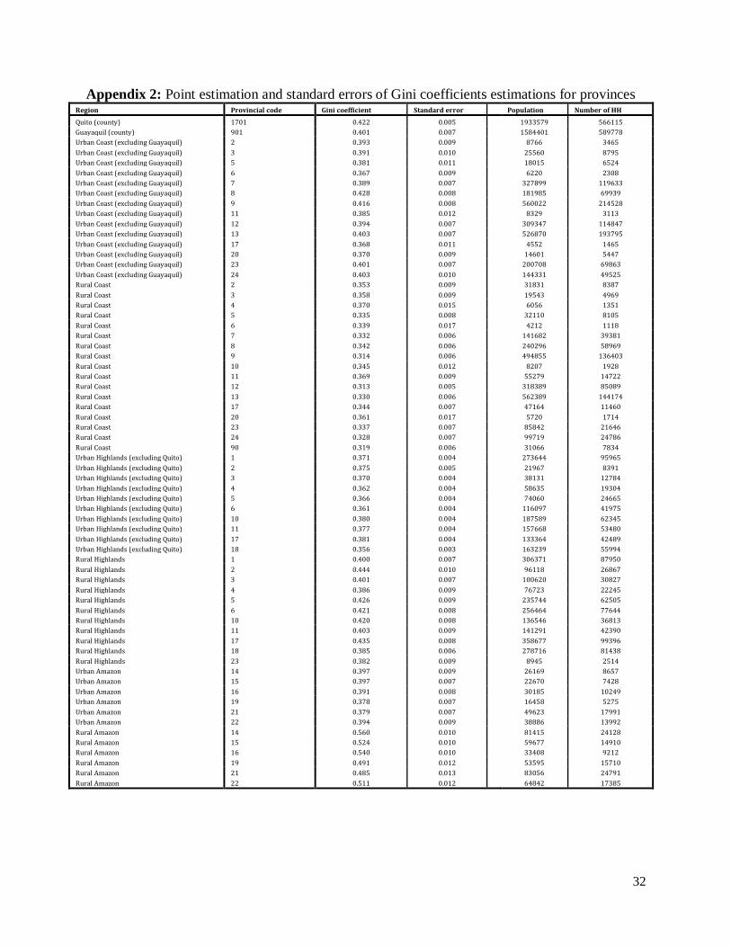
32

Appendix 2: Point estimation and standard errors of Gini coefficients estimations for provinces Region Provincial code Gini coefficient Standard error Population Number of HH

Quito (county) 1701 0.422 0.005 1933579 566115

Guayaquil (county) 901 0.401 0.007 1584401 589778

Urban Coast (excluding Guayaquil) 2 0.393 0.009 8766 3465

Urban Coast (excluding Guayaquil) 3 0.391 0.010 25560 8795

Urban Coast (excluding Guayaquil) 5 0.381 0.011 18015 6524

Urban Coast (excluding Guayaquil) 6 0.367 0.009 6220 2308

Urban Coast (excluding Guayaquil) 7 0.389 0.007 327899 119633

Urban Coast (excluding Guayaquil) 8 0.428 0.008 181985 69939

Urban Coast (excluding Guayaquil) 9 0.416 0.008 560022 214528

Urban Coast (excluding Guayaquil) 11 0.385 0.012 8329 3113

Urban Coast (excluding Guayaquil) 12 0.394 0.007 309347 114847

Urban Coast (excluding Guayaquil) 13 0.403 0.007 526870 193795

Urban Coast (excluding Guayaquil) 17 0.368 0.011 4552 1465

Urban Coast (excluding Guayaquil) 20 0.370 0.009 14601 5447

Urban Coast (excluding Guayaquil) 23 0.401 0.007 200708 69863

Urban Coast (excluding Guayaquil) 24 0.403 0.010 144331 49525

Rural Coast 2 0.353 0.009 31831 8387

Rural Coast 3 0.358 0.009 19543 4969

Rural Coast 4 0.370 0.015 6056 1351

Rural Coast 5 0.335 0.008 32110 8105

Rural Coast 6 0.339 0.017 4212 1118

Rural Coast 7 0.332 0.006 141682 39381

Rural Coast 8 0.342 0.006 240296 58969

Rural Coast 9 0.314 0.006 494855 136403

Rural Coast 10 0.345 0.012 8207 1928

Rural Coast 11 0.369 0.009 55279 14722

Rural Coast 12 0.313 0.005 318389 85089

Rural Coast 13 0.330 0.006 562389 144174

Rural Coast 17 0.344 0.007 47164 11460

Rural Coast 20 0.361 0.017 5720 1714

Rural Coast 23 0.337 0.007 85842 21646

Rural Coast 24 0.328 0.007 99719 24786

Rural Coast 90 0.319 0.006 31066 7834

Urban Highlands (excluding Quito) 1 0.371 0.004 273644 95965

Urban Highlands (excluding Quito) 2 0.375 0.005 21967 8391

Urban Highlands (excluding Quito) 3 0.370 0.004 38131 12784

Urban Highlands (excluding Quito) 4 0.362 0.004 58635 19304

Urban Highlands (excluding Quito) 5 0.366 0.004 74060 24665

Urban Highlands (excluding Quito) 6 0.361 0.004 116097 41975

Urban Highlands (excluding Quito) 10 0.380 0.004 187589 62345

Urban Highlands (excluding Quito) 11 0.377 0.004 157668 53480

Urban Highlands (excluding Quito) 17 0.381 0.004 133364 42489

Urban Highlands (excluding Quito) 18 0.356 0.003 163239 55994

Rural Highlands 1 0.400 0.007 306371 87950

Rural Highlands 2 0.444 0.010 96118 26867

Rural Highlands 3 0.401 0.007 100620 30827

Rural Highlands 4 0.386 0.009 76723 22245

Rural Highlands 5 0.426 0.009 235744 62505

Rural Highlands 6 0.421 0.008 256464 77644

Rural Highlands 10 0.420 0.008 136546 36813

Rural Highlands 11 0.403 0.009 141291 42390

Rural Highlands 17 0.435 0.008 358677 99396

Rural Highlands 18 0.385 0.006 278716 81438

Rural Highlands 23 0.382 0.009 8945 2514

Urban Amazon 14 0.397 0.009 26169 8657

Urban Amazon 15 0.397 0.007 22670 7428

Urban Amazon 16 0.391 0.008 30185 10249

Urban Amazon 19 0.378 0.007 16458 5275

Urban Amazon 21 0.379 0.007 49623 17991

Urban Amazon 22 0.394 0.009 38886 13992

Rural Amazon 14 0.560 0.010 81415 24128

Rural Amazon 15 0.524 0.010 59677 14910

Rural Amazon 16 0.540 0.010 33408 9212

Rural Amazon 19 0.491 0.012 53595 15710

Rural Amazon 21 0.485 0.013 83056 24791

Rural Amazon 22 0.511 0.012 64842 17385

33

Appendix 3: Housing conditions index

We use the first component as our housing conditions index. The index increases as the living conditions improve.

Component Matrixa

Component

1 2

Dummy houses with a sewage connection .784 -.228 Dummy houses with public garbage collection services .765 -.081 Dummy houses with exclusive washroom .726 -.211 Dummy houses with electricity .465 .536 Dummy houses with viable walls .622 .368 Dummy houses with viable floors .694 .207 Dummy houses with a water connection .770 -.097 Dummy houses with viable roof .232 .605 Dummy houses with phone connection .657 -.287 Dummy houses with overcrowding -.302 .349

Extraction Method: Principal Component Analysis. a. 2 components extracted.

Total Variance Explained

Component

Initial Eigenvalues Extraction Sums of Squared Loadings

Total % of Variance Cumulative % Total % of Variance Cumulative %

1 3.980 39.803 39.803 3.980 39.803 39.803 2 1.149 11.489 51.293 1.149 11.489 51.293 3 .935 9.352 60.645 4 .875 8.748 69.393 5 .766 7.656 77.049 6 .673 6.726 83.775 7 .482 4.821 88.596 8 .448 4.484 93.080 9 .371 3.713 96.792 10 .321 3.208 100.000

Extraction Method: Principal Component Analysis.

Results of principal component analysis of housing conditions

Sub-region Mean N Std. Deviation

Quito 0.9154 496527 .38313230 Guayaquil 0.4493 541943 .70698084 Sierra Urbana sin Quito 0.7367 437262 .56331707 Sierra Rural -0.4467 585807 .81424722 Costa Urbana sin Guayaquil 0.2085 632177 .75130373 Costa Rural -1.0964 434422 .69612512 Amazonia Urbana 0.2571 44380 .80840630 Amazonia Rural -1.0525 92347 1.05149895 Total 0.1005 3264866 .96987113

34

Appendix 4: Food consumption index

We use the second factor component of this analysis as a control variable in our models. This factor assigns high values to households with high consumption of carbohydrates such as tubers.

Component Matrixa

Component

1 2 3 4 5 6

Total calories consumed on average (parish) .658 -.256 .252 .363 -.132 .130 Carbohydrates from cereal: gr per day consumed on average in every parish .403 -.350 .463 .422 -.149 .362 Carbohydrates from fruit: gr per day consumed on average in every parish .628 .240 -.225 -.121 -.619 -.129 Carbohydrates from milk and derivatives: gr or ml per day consumed on average in every parish .665 -.005 -.465 -.302 .152 .314 Carbohydrates from legumes: gr per day consumed on average in every parish .462 .131 .701 -.502 .056 -.093 Total carbohydrates: gr or ml per day consumed on average in every parish .714 -.071 .412 .342 -.230 .263 Carbohydrates from tubers: gr per day consumed on average in every parish .124 .908 .054 .189 .107 .183 Carbohydrates from vegetables: gr per day consumed on average in every parish .766 .025 -.032 .297 .341 -.369 Fat from meats and derivatives: gr per day consumed on average in every parish .779 -.029 -.143 .005 .061 -.003 Fat from fruit: gr per day consumed on average in every parish .746 .160 -.314 -.046 -.420 -.152 Fat from milk and derivatives: gr per day consumed on average in every parish .691 -.109 -.390 -.406 .207 .333 Fat from fats and oils: gr per day consumed on average in every parish .268 -.337 .531 .156 -.029 .101 Fat from legumes: gr per day consumed on average in every parish .431 .225 .702 -.469 .015 -.117 Fat from tubers: gr per day consumed on average in every parish .061 .937 .042 .223 .112 .188 Fat from vegetables: gr per day consumed on average in every parish .808 .049 -.117 .247 .312 -.342 Protein from meats and derivatives: gr per day consumed on average in every parish .779 .024 -.163 .030 .092 -.008 Protein from fruit: gr per day consumed on average in every parish .725 .209 -.282 -.088 -.551 -.152 Protein from milk and derivatives: gr or ml per day consumed on average in every parish .686 -.135 -.366 -.411 .209 .325 Protein from legumes: gr per day consumed on average in every parish .453 .205 .715 -.459 .065 -.088 Protein from fish and seafood: gr per day consumed on average in every parish .385 -.551 -.002 .100 .147 .060 Total protein: gr per day consumed on average in every parish .915 -.112 .101 .183 .015 .135 Protein from tubers: gr per day consumed on average in every parish .042 .928 .037 .226 .110 .184 Protein from vegetables: gr per day consumed on average in every parish .832 .001 -.091 .215 .293 -.349

Extraction Method: Principal Component Analysis. a. 6 components extracted.

Total Variance Explained

Component

Initial Eigenvalues Extraction Sums of Squared Loadings

Total % of Variance Cumulative % Total % of Variance Cumulative %

1 8.797 38.248 38.248 8.797 38.248 38.248 2 3.458 15.035 53.283 3.458 15.035 53.283 3 3.041 13.220 66.504 3.041 13.220 66.504 4 1.960 8.524 75.028 1.960 8.524 75.028 5 1.443 6.275 81.303 1.443 6.275 81.303 6 1.134 4.932 86.235 1.134 4.932 86.235

Extraction Method: Principal Component Analysis.

Results of principal component analysis of food consumption index Sub-region Mean N Std. Deviation

Quito 0.5279 424982 .0000000 Guayaquil -1.0238 541943 .0000000 Urban highlands 0.4880 594103 1.0451720 Rural highlands 1.1804 489298 1.8296341 Urban coast -1.4320 759663 .4421891 Rural coast -1.8843 306937 .7794456 Urban Amazon -0.3765 56187 .6162099 Rural Amazon -0.3728 67627 .7688065 Total National -0.3627 3240740 1.4087608

List of food items and their food groups

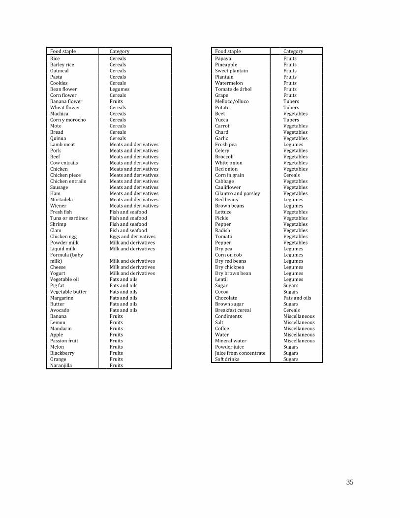
35

Food staple Category

Rice Cereals Barley rice Cereals Oatmeal Cereals Pasta Cereals Cookies Cereals Bean flower Legumes Corn flower Cereals Banana flower Fruits Wheat flower Cereals Machica Cereals Corn y morocho Cereals Mote Cereals Bread Cereals Quinua Cereals Lamb meat Meats and derivatives Pork Meats and derivatives Beef Meats and derivatives Cow entrails Meats and derivatives Chicken Meats and derivatives Chicken piece Meats and derivatives Chicken entrails Meats and derivatives Sausage Meats and derivatives Ham Meats and derivatives Mortadela Meats and derivatives Wiener Meats and derivatives Fresh fish Fish and seafood Tuna or sardines Fish and seafood Shrimp Fish and seafood Clam Fish and seafood Chicken egg Eggs and derivatives Powder milk Milk and derivatives Liquid milk Milk and derivatives Formula (baby milk) Milk and derivatives Cheese Milk and derivatives Yogurt Milk and derivatives Vegetable oil Fats and oils Pig fat Fats and oils Vegetable butter Fats and oils Margarine Fats and oils Butter Fats and oils Avocado Fats and oils Banana Fruits Lemon Fruits Mandarin Fruits Apple Fruits Passion fruit Fruits Melon Fruits Blackberry Fruits Orange Fruits Naranjilla Fruits

Food staple Category

Papaya Fruits Pineapple Fruits Sweet plantain Fruits Plantain Fruits Watermelon Fruits Tomate de árbol Fruits Grape Fruits Melloco/olluco Tubers Potato Tubers Beet Vegetables Yucca Tubers Carrot Vegetables Chard Vegetables Garlic Vegetables Fresh pea Legumes Celery Vegetables Broccoli Vegetables White onion Vegetables Red onion Vegetables Corn in grain Cereals Cabbage Vegetables Cauliflower Vegetables Cilantro and parsley Vegetables Red beans Legumes Brown beans Legumes Lettuce Vegetables Pickle Vegetables Pepper Vegetables Radish Vegetables Tomato Vegetables Pepper Vegetables Dry pea Legumes Corn on cob Legumes Dry red beans Legumes Dry chickpea Legumes Dry brown bean Legumes Lentil Legumes Sugar Sugars Cocoa Sugars Chocolate Fats and oils Brown sugar Sugars Breakfast cereal Cereals Condiments Miscellaneous Salt Miscellaneous Coffee Miscellaneous Water Miscellaneous Mineral water Miscellaneous Powder juice Sugars Juice from concentrate Sugars Soft drinks Sugars