making the right moves: guiding alpha-expansion using
TRANSCRIPT
Making the Right Moves:Guiding Alpha-Expansion using Local Primal-Dual Gaps
Dhruv BatraToyota Technological Institute at Chicago
Pushmeet KohliMicrosoft Research Cambridge
Abstract
This paper presents a new adaptive graph-cut basedmove-making algorithm for energy minimization. Tradi-tional move-making algorithms such as Expansion andSwap operate by searching for better solutions in some pre-defined moves spaces around the current solution. In con-trast, our algorithm uses the primal-dual interpretation ofthe Expansion-move algorithm to adaptively compute thebest move-space to search over. At each step, it tries togreedily find the move-space that will lead to biggest de-crease in the primal-dual gap. We test different variantsof our algorithm on a variety of image labelling problemssuch as object segmentation and stereo. Experimental re-sults show that our adaptive strategy significantly outper-forms the conventional Expansion-move algorithm, in somecases cutting the runtime by 50%.
1. Introduction
Graph-cut based move-making algorithms such as Ex-pansion and Swap [4] are extremely popular in computervision. They enable researchers to efficiently computeapproximate maximum a posteriori (MAP) solutions ofMarkov and Conditional Random Fields (MRFs, CRFs),and are used for solving a wide variety of labelling prob-lems such as image segmentation [3,19,21], object-specificsegmentation [2, 8, 26], geometric labelling [10, 20], imagedenoising/inpainting [9,24,28], stereo [4,22,31] and opticalflow [4, 6].
Classical move-making algorithms such as Expansionand Swap operate by making a series of changes to the so-lution. These changes (also called moves) are performedsuch that they do not lead to an increase in the solutionenergy. Convergence is achieved when the energy cannotbe decreased any further. In each iteration, the algorithmsearches for a lower energy solution in a pre-defined neigh-borhood (also called the move space) around the current so-lution. It is important to draw a distinction between moves
0 20 40 600
1
2
3x 10⁴
# Disparity Labels in an image
# Pi
xels
(a) Cones
0 5 10
4
6
8
x 107
Time (sec.)
Ener
gy
Standard ExpansionLPDG Partial Sweep
(b) Cones
1 2 3 4 5 6 7 8 9 100
50
100
150
200
# Im
ages
# Objects in an Image
(c) PASCAL
1 2 3 4 5 6 70
50
100
150
200
250
# Im
ages
# Objects in an Image
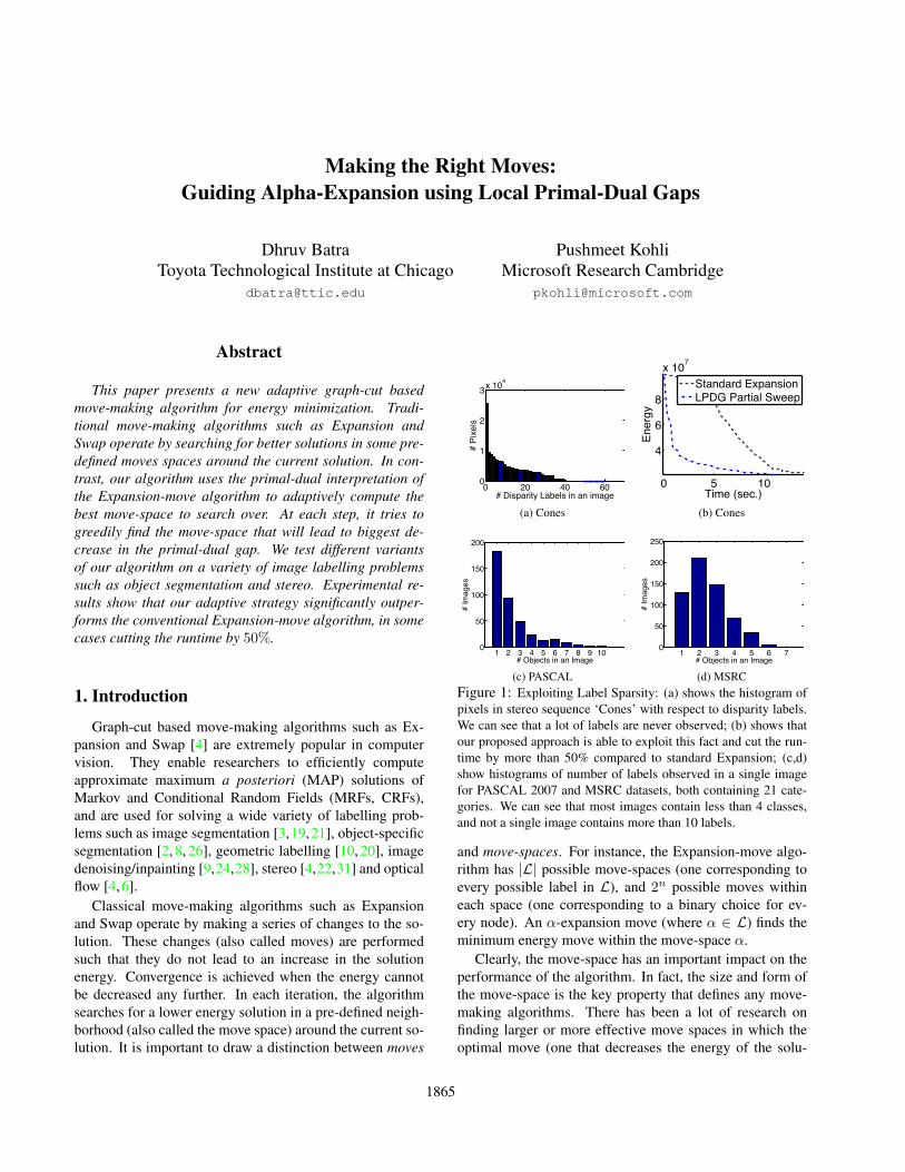
(d) MSRCFigure 1: Exploiting Label Sparsity: (a) shows the histogram ofpixels in stereo sequence ‘Cones’ with respect to disparity labels.We can see that a lot of labels are never observed; (b) shows thatour proposed approach is able to exploit this fact and cut the run-time by more than 50% compared to standard Expansion; (c,d)show histograms of number of labels observed in a single imagefor PASCAL 2007 and MSRC datasets, both containing 21 cate-gories. We can see that most images contain less than 4 classes,and not a single image contains more than 10 labels.
and move-spaces. For instance, the Expansion-move algo-rithm has |L| possible move-spaces (one corresponding toevery possible label in L), and 2n possible moves withineach space (one corresponding to a binary choice for ev-ery node). An α-expansion move (where α ∈ L) finds theminimum energy move within the move-space α.
Clearly, the move-space has an important impact on theperformance of the algorithm. In fact, the size and form ofthe move-space is the key property that defines any move-making algorithms. There has been a lot of research onfinding larger or more effective move spaces in which theoptimal move (one that decreases the energy of the solu-
1865

0 1 2 3 4
1.71.81.9
22.12.22.32.4
x 108
Time (sec.)
Ener
gy
Standard ExpansionLPDG
0 2 4 6 8
1
1.5
2
2.5x 10⁸
Time (sec.)
Ener
gy
Standard ExpansionLPDG
0 1 2 35
5.5
6
6.5
7
7.5
8x 10⁷
Time (sec.)
Ener
gy
Standard ExpansionLPDG
Ordering of Expanded Labels
Move Number Classical
Expansions Our Guided Expansions
Image 1 1 Airplane Car
2 Bicycle Person
3 Bird Motorbike
4 Boat Train
5 Bo6le Airplane
Image 2 1 Airplane Sheep
2 Bicycle Dog
3 Bird Bird
4 Boat Cow
5 Bo6le Cat
Image 3 1 Airplane Airplane
2 Bicycle Bird
3 Bird Dog
4 Boat TV
5 Bo6le Train
Figure 2: The first column of the figure shows three images from the dataset used for the PASCAL visual object category (VOC) challenge2009. We used the pairwise energy functions for this problem used by [17]. The second column shows the first five labels used for expansionmoves by the standard algorithm and our guided variant. It can be seen that our algorithm is able to propose labels relevant to the probleminstance (marked in bold). The third column shows graphs of how the energy of the solutions obtained by standard Expansion and ourguided variant changes with time. It can be seen that our algorithm consistently outperforms the standard Expansion algorithm.
tion by the most amount) can be computed in polynomialtime [7, 16, 18, 29, 32].
However, there has been surprisingly little work on de-termining what is the best move space to search over, giventhe current solution and a family of move spaces. For in-stance, in the case of the Expansion algorithm, the standardapproach is to iterate over the move spaces correspondingto different labels one after the other in a pre-specified orrandom order. This strategy is energy-oblivious and doesnot exploit the knowledge that certain labels are more prob-able to occur in the image and thus expanding them maylead to lower energies. Further, the standard Expansion al-gorithm makes complete sweeps over the label set. In manylabelling problems, only a few labels are assigned in theMAP solution. This is particularly true in the case of objectsegmentation problems. Fig. 1 shows that individual im-ages in the popular MSRC [26] (21 object labels) and PAS-CAL Visual Object Category dataset [5] (20 foreground and1 background labels) contain very few labels. Specifically,even though both dataset contain 21 labels, most imagescontain less than 4 labels, and no image contains more than10 labels. This certainly begs the question – why would wewant to repeatedly iterate over all possible labels within theExpansion-move algorithm?
Contributions. In this paper, we propose an adaptivemove-making algorithm that tries to find the best movespace to search over in each iteration. Our algorithm triesto greedily find the label α for which the corresponding α-expansion move will lead to the most decrease in the energy.The labels chosen for some object segmentation problemsare shown in Fig. 2. We can see that the labels chosen byour algorithm for Expansion are more meaningful and spe-cific to the images. The figure also shows that the guidedExpansion algorithm is able to find a lower-energy solutionmuch more quickly compared to the standard method.
Our algorithm is inspired from the primal-dual interpre-tation of the Expansion algorithm given by Komodakis etal. [15, 16]. Komodakis and Tziritas [15] proposed threegraph-cut-based primal-dual algorithms namely, PD1, PD2and PD3 for performing MAP inference. Furthermore, theyshowed that one of their algorithms (PD3) has the exactsame steps as that of the Expansion algorithm. Thus, theExpansion algorithm can be seen as solving a well knownLinear Programming (LP) relaxation (and its correspondingdual) of the energy minimization problem.
The energy of the current solution and the achieved ob-jective of the LP-dual provides upper and lower boundsrespectively on the energy of the optimal solution. Fur-
1866

thermore, the difference between these values (called theprimal-dual gap) provides a quantitative measure of the ac-curacy of the current solution. In fact, state-of-the-art LP-based methods for MAP inference [27] operate by incre-mentally tightening the relaxation to reduce the primal-dualgap. In the context of move-making algorithms, the aboveargument would lead to a strategy where we search for theoptimal move in the move space that will lead to the biggestdecrease in the primal-dual gap.
Finding the best move space is a difficult problem. Forinstance, to find out the best move space for Expansionna ively, one may need to try out all possible move spaces,i.e. one per label in the label set. This is a computationallyexpensive operation and would make the algorithm imprac-tical for large labels spaces (e.g. in denoising applications).The key observation of this paper is that a good approxima-tion to the relative drop in the primal-dual gap correspond-ing to different Expansion move spaces can be constructedusing the primal and dual variables of the LP formulationof the problem. This approach is extremely efficient andruns in linear time in the number of variables and labels.We test the efficacy of our method on a number of imagelabelling problems. The experimental results show that ouradaptive method significantly outperforms the widely usedtraditional Expansion-move algorithm.
2. Related Work
The last few years have seen the proposal of a number ofsophisticated methods to improve the efficiency of move-making algorithms such as Expansion [1, 16, 18, 32]. Thesemethods can be divided into two broad categories: energy-oblivious and energy-aware.
Energy-oblivious methods do not use the knowledge ofthe energy function to reduce computation time. The FAST-PD algorithm proposed by Komodakis et al. [16] and a re-lated but simpler algorithm proposed by Alahari et al. [1]are two such methods. They use results of initial iterationsof the Expansion algorithm to make subsequent iterationsfaster, and are inspired from the the dynamic graph cuts al-gorithm proposed by Kohli and Torr [13]. Another exampleis the fusion-move algorithm [18, 32]. This algorithm usesproposal solutions of the labeling problem obtained fromdifferent methods for defining the move space for the movemaking algorithm.
Our algorithm belongs to the class of energy-aware tech-niques which use the energy function to guide the search.The only other method which belongs to this class isthe gradient-descent fusion-move algorithm proposed byIshikawa [11]. This method tries to find the most promis-ing move-space to search over by using the gradient of theenergy function.
3. Notation and PreliminariesWe start by providing the notation used in the
manuscript. For any positive integer n, let [n] be shorthandfor the set {1, 2, . . . , n}. We consider a set of discrete ran-dom variables x = {xi | i ∈ [n]}, each taking value in afinite label set xi ∈ L = [k]. Let G = (V, E) be a graphdefined over these variables, i.e. V = [n], E ⊆
([n]2
). The
goal of MAP inference is to find the labelling x of the vari-ables which minimize a real-valued energy function associ-ated with this graph:
minx∈Ln
E(x) = minx∈Ln
∑i∈V
θi(xi) +∑
(i,j)∈E
θij(xi, xj)
, (1)
where θi(·), θij(·, ·) denote node and edge energies.
3.1. The Expansion-Move Algorithm
The Expansion algorithm starts with an initial solutionand proceeds by making a series of changes which lead tosolutions having lower energy. An α-expansion move overa label α ∈ L allows any random variable to either retainits current label or take label α. One sweep of the algo-rithm involves making moves for all α ∈ L in some ordersuccessively.
The optimalα-expansion move can be computed in poly-nomial time if the pairwise energy parameters θij define ametric, i.e.
θij(a, b) = 0 ⇐⇒ a = b, (2a)θij(a, b) = θij(b, a) ≥ 0 (2b)θij(a, c) ≤ θij(a, b) + θij(b, c), ∀a, b, c ∈ L. (2c)
In this work, we do not assume the pairwise energies to bemetrics. We only require: θij(a, a) = 0, ∀a and θij(a, b) ≥0.
3.2. MAP Integer Program
MAP inference is typically set up as an integer pro-gramming problem over the boolean variables. Letµi(s), µij(s, t) ∈ {0, 1} be indicator variables, such that{µi(s) = 1 ⇔ xi = s}, and {µij(s, t) = 1 ⇔ xi =s, xj = t}. Moreover, let µi = {µi(s) | s ∈ L},θi ={θi(s) | s ∈ L} be vectors of indicator-variables and en-ergies for node i. Let µij and θij be defined analogously.Using this notation, the MAP inference integer program canbe written as:
minµi,µij
∑i∈V
θi · µi +∑
(i,j)∈E
θij · µij (3a)
s.t.∑s∈L
µi(s) = 1 ∀i ∈ V (3b)∑s∈L
µij(s, t) = µj(t) ∀(i, j), (j, i) ∈ E (3c)
µi(s), µij(s, t) ∈ {0, 1}. (3d)
1867

θij(·, ·)
hi(xpi )
hi(α)
hj(α)
hj(xpj )
+δ−δ
Figure 3: Interpretation of dual variables. See text for details
Problem (3) is known to be NP-hard in general [25].The standard LP relaxation of this problem, also knownas Schlesingers bound [23, 30], is given by relaxingthe boolean constraints (3d) to the unit interval, i.e.µi(s), µij(s, t) ≥ 0.
3.3. The Primal-Dual Interpretation of Expansion
Komodakis et al. [15, 16] gave a primal-dual interpreta-tion of α-expansion. Since our contribution builds on theirinterpretation, we briefly review their work here.
The LP-dual of (3) that Komodakis et al. [15, 16] choseto work with was:
maxhi,yij(t)
∑i∈V
hi (4)
s.t. hi ≤ hi(s) ∀i ∈ V, syij(t) + yji(s) ≤ θij(s, t) ∀(i, j) ∈ E , s, thi, yij(t) ∈ R,
where hi(s).= θi(s) +
∑j∈N (i) yji(s), where N (i) =
{j | (i, j) ∈ E} is the set of neighbours of node i.Every feasible dual solution provides a lower-bound on
the MAP value, i.e.:E(x) ≥ E(x∗) ≥
∑i∈V
hi (5)
Moreover, for any primal labelling xp, the quantity Primal-Dual Gap (E(xp)−∑i∈V hi) gives an estimate of the tight-ness of the relaxation. Specifically, a pair of primal-dualsolutions (xp, {hi, hi(·), yij(·)}) is an f -approximate solu-tion iff:
E(xp) =∑i∈V
θi(xpi ) +
∑(i,j)∈E
θij(xpi , x
pj ) ≤ f
(∑i∈V
hi
)(6)
Komodakis et al. [15, 16] proposed two primal-dual al-gorithms called PD3 [15] and FastPD [16]1 that wereboth shown to be equivalent to α-expansion. These al-gorithms are based on a particular set of relaxed com-plementary slackness conditions for the primal-dual pro-grams. Specifically, if we define dmax
.= maxij,s,t θij(s, t)
and dmin.= minij,s 6=t θij(s, t), a pair of primal-dual solu-
tions (xp, {hi, hi(·), yij(·)}) achieves an fapp = 2 · dmax
dmin-
approximation ratio iff [14, 15]:1FastPD is a faster version of PD3.
hi(xpi ) = min
s∈Lhi(s) (7a)
yij(xpj ) + yji(x
pi ) = θij(xi, xj) (7b)
yij(t) + yji(s) ≤ 2θij(s, t) (7c)
Intuitive Interpretation + Example: An intuitive in-terpretation of the dual variables helps in understand-ing these constraints. Fig. 3 shows the dual variableshi(x
pi ), hi(α), hj(x
pj ), hj(α) associated with an edge (i, j).
The cost of each node-label pair is represented by a ballwith that height. Condition (7a) requires that the height ofball corresponding to primal labelling be the lowest. Wecan see that this is satisfied for node j but not for nodei, where hi(α) < hi(x
pi ). Recall that hi(s) = θi(s) +∑
j∈N (i) yji(s). Thus, we may increase the height of α atnode i, hi(α), by increasing the dual variable yji, i.e. by set-ting yji(α)← yji(α) + δ. However, constraint (7c) forces:
yij(α) + yji(α) ≤ 2θij(α, α) = 0 (8)⇒ yij(α) ≤ −yji(α). (9)
Thus, increasing hi(α) decreases hj(α) by at least the sameamount, i.e., hj(α) ← hj(α) − δ. In this example, thischange increased the dual by +δ, i.e. hi+hj ← hi+hj+δ.
For a general graph, both algorithms – PD3 [15] andFastPD [16] – operate in a block-coordinate ascent fashion.They loop over labels in a pre-determined order and at eachstep optimize all dual-variables corresponding to a label α,while holding all other dual variables fixed.
• Loop on label α ∈ L:
–α-expansion: Update {hi, hi(α), yij(α), yji(α)};Update {xpi |xpi = α}.
In both algorithms, conditions (7b), (7c) are satisfied byconstruction, and the goal of these block-updates is to makeprogress on condition (7a), i.e. to extract a primal labellingthat has the minimal height at all nodes. We refer the readerto Komodakis et al. [15, 16] for details of the update steps.
4. Adaptive Primal-Dual Expansion MovesIn this paper we focus on how to enumerate over the la-
bels for primal-dual Expansion moves. Typical choices areto loop over labels one after the other in a pre-specified orrandom order. This is exactly the scheme that FastPD fol-lows. We follow an energy-aware strategy that uses the pri-mal and dual variables to make adaptive Expansion moves.Specifically, we present a label proposal heuristic that sortslabels according to a scoring function that quantifies howhelpful a label will be for α-expansion. Our label scoringfunction is derived from complementary slackness condi-tion (7a).
1868

Algorithm 1 LPDG-Sweep1: for t = 0, 1, . . . do2: Compute LPDG-based label scores ω(·) ∈
{ω1(·), ω2(·), ω3(·)}.3: Sort label scores: {α1, . . . , αk} = sort(ω(·))4: for i = 1, . . . , k do5: αi-expansion: Update variables:
{hi, hi(α), yij(α), yji(α)}6: end for7: end for
4.1. Local Primal-Dual Gap
We first define a quantity we call Local Primal-Dual Gap(LPDG) for every label and variable. Given a pair of primal-dual solutions (xp, {hi, hi(·), yij(·)}), LPDG is formallydefined as:
lpdg(α, i) = hi(xpi )− hi(α). (10)
Using the ball analogy of dual variables from Fig. 3 again,LPDG can be seen as the height difference between the ballsat node i corresponding to the primal labelling xpi and thelabel α. Positive values of LPDG indicate violations ofcomplementary slackness, and we can say that dual vari-able hi(α) is in deficit by an amount of lpdg(α, i). Neg-ative values of LPDG indicate that complementary slack-ness is satisfied and that dual variable hi(α) is in surplus byamount lpdg(α, i). A dual variable in deficit hi(α) needs tobe “fixed” by the algorithm and a neighbouring dual vari-able in surplus hj(α), j ∈ N (i) can help this process byvia the message-variables yij(α), yji(α). Thus, lpdg(α, i)quantifies the amount of violation in complementary slack-ness conditions at node i, label α, and lpdg(α, j) quanti-fies how much node j can help correct this violation. Morespecifically, we can state the following property of LPDG:
Proposition 1 Slackness: If LPDG for all nodes is non-positive, i.e. lpdg(α, i) ≤ 0, ∀i ∈ V, α ∈ L, then comple-mentary slackness conditions hold and we have achieved anfapp-approximate solution.
4.2. LPDG-based Label Scoring Functions
LPDG gives us an appropriate language to describe ourgoals for label scoring. In order to get the highest dropin primal-dual gap, we need to pick a label α that has themost deficit. However, we also need to make sure there isenough surplus so that we may actually make an improve-ment. Keeping this in mind, we propose the following threelabel scoring functions:
• LPDG-crisp:ω1(α) =
∑i∈V I[0∞) (lpdg(α, i)),
where IS(y) ={
1 y ∈ S0 else (11)
Algorithm 2 LPDG-Partial-Sweep1: for t = 0, 1, . . . do2: Compute LPDG-based label scores ω(·) ∈
{ω1(·), ω2(·), ω3(·)}.3: Find highest label score: α = argmaxα ω(α)4: α-expansion: Update variables:
{hi, hi(α), yij(α), yji(α)}5: end for
• LPDG-deficit:ω2(α) =
∑i∈V lpdg(α, i) · I[0∞) (lpdg(α, i))
• LPDG-tradeoff:ω3(α) =
∑i∈V
∣∣lpdg(α, i)∣∣LPDG-crisp ignores the actual LPDG values and sim-
ply counts the number of nodes in deficit. LPDG-deficit onthe other hand also incorporates the how much these nodesare in deficit. Finally, LPDG-tradeoff incorporates both theamount of deficit and the surplus over all nodes.
Finally, we propose the following two adaptive primal-dual Expansion algorithms: 1) LPDG-Sweep, shown inAlg 1 that uses an LPDG-scoring-function-based permuta-tion of labels to perform α-expansion in each sweep, and2) LPDG-Partial-Sweep, show in Alg. 2, that performs par-tial sweeps where LPDG-based reordering of labels is per-formed after each alpha-expansion.
The standard Expansion algorithm goes through all la-bels in one iteration, and thus has a linear runtime com-plexity in the number of labels in the problem. This makesit inefficient on problems with very large label sets. Ourpartial-sweep scheme based on LPDG scores is not boundto the linear complexity and only expands labels which arerelevant to the problem instance.
5. Experiments
We evaluated our method on the problems of object seg-mentation and stereo matching.Stereo: We use image pairs from the Middlebury StereoDataset.2 We used the energy function made available byAlahari et al. [1]. The number of disparity labels in differentproblem instances were: Tsukuba (16), Venus (20), Cones(60) and Teddy (60).Object Segmentation: For this application, we usedthe pairwise energy functions constructed by Ladicky etal. [17] that are based on the method of Shotton etal. [26]. We tested our algorithm on some images from theMSRC [26] (21 object labels) and PASCAL Visual ObjectCategory dataset [5] (20 foreground and 1 background la-bels) datasets.
2http://vision.middlebury.edu/stereo/data/.
1869

0 1 2 3 4x 10⁷
0
2
4
6
8
10x 104
LPDG crisp
Dec
reas
e in
Prim
al
(a) LPDG-crisp.
0 1 2 3 4x 10⁷
0
1
2
3
4x 10⁷
LPDG deficit
Dec
reas
e in
Prim
al(b) LPDG-deficit.
0 1 2 3 4x 10⁷
0
1
2
3
4
5x 10⁷
LPDG tradeoff
Dec
reas
e in
Prim
al
(c) LPDG-tradeoff.
1 2 3 4 50.2
0
0.2
0.4
0.6
0.8
1
1.2
# Expansions
Cor
rela
tion
Coe
ffien
t
LPDG crispLPDG deficitLPDG tradeoff
(d) Correlation Coefficients.
Figure 4: Correlation between LPDG-based scores and decrease in energy. Graph (a) shows the relationship between the true de-crease in energy and the LPDG-crisp score. Each point on the graph corresponds to a proposed label-expansion at the start of the energyminimization procedure. The x-axes shows what was the LPDG-crisp score for the particular label expansion, while the y-axes shows whatwas the decrease in the energy of the solution when this label-expansion was performed. Graphs (b) and (c) show the corresponding plotsfor the LPDG-deficit and LPDG-trade-off scores respectively. It can be seen that all scores are highly correlated at the start. Graph (d)shows that the correlation between the LPDG scores and the decrease in the energy falls as we perform more expansion moves.
Correlation between LPDG-ranking and True-rankingTo quantify the performance of our LPDG-based metricsin predicting usefulness of labels, we measure the correla-tion between the proposed label LPDG scores and the truedecrease in the primal energy. To do this, we performedthe following experiment: we first let k sweeps of alpha-expansion occur in the usual fashion (i.e., in some staticpre-fixed ordering over the variables). After the comple-tion of these k standard sweeps, we loop over all labels andfor each label l we record all three of our label scores andalso record the drop in energy if this label was expandedon immediately after finishing the k standard sweeps. Fig 4shows the correlation plots for the k = 0 case, i.e. withoutany sweeps. We can see a very strong correlation for allthree of our label scores. Fig 4 also shows the correlationcoefficient as a function of k. We can see that the correla-tion is very high initially and then slows decays away as theproblem moves towards convergence. However, it is impor-tant to remember that with methods like FastPD it is the firstfew iterations that are responsible for most of the time takenby the algorithm and this is precisely where LPDG is mosthelpful.Comparison with FAST-PD. We compare the performanceof our method with the FAST-PD algorithm proposed byKomodakis et al. [16], which is an efficient version of thestandard Expansion algorithm. To ensure our experimentsassess the relative performance of our proposed LPDGscores and are not influenced by the particular details ofthe primal-dual alpha-expansion implementation, we usethe use the implementation provided by Komodakis et al.for all our experiments.3 All methods reported in this pa-per differ only in the order of expansions and thus the rel-ative performance differences can be directly attributed toour improved score function.
Fig. 5 shows the energy-vs-iteration and energy-vs-time
3http://www.csd.uoc.gr/˜komod/FastPD/index.html.
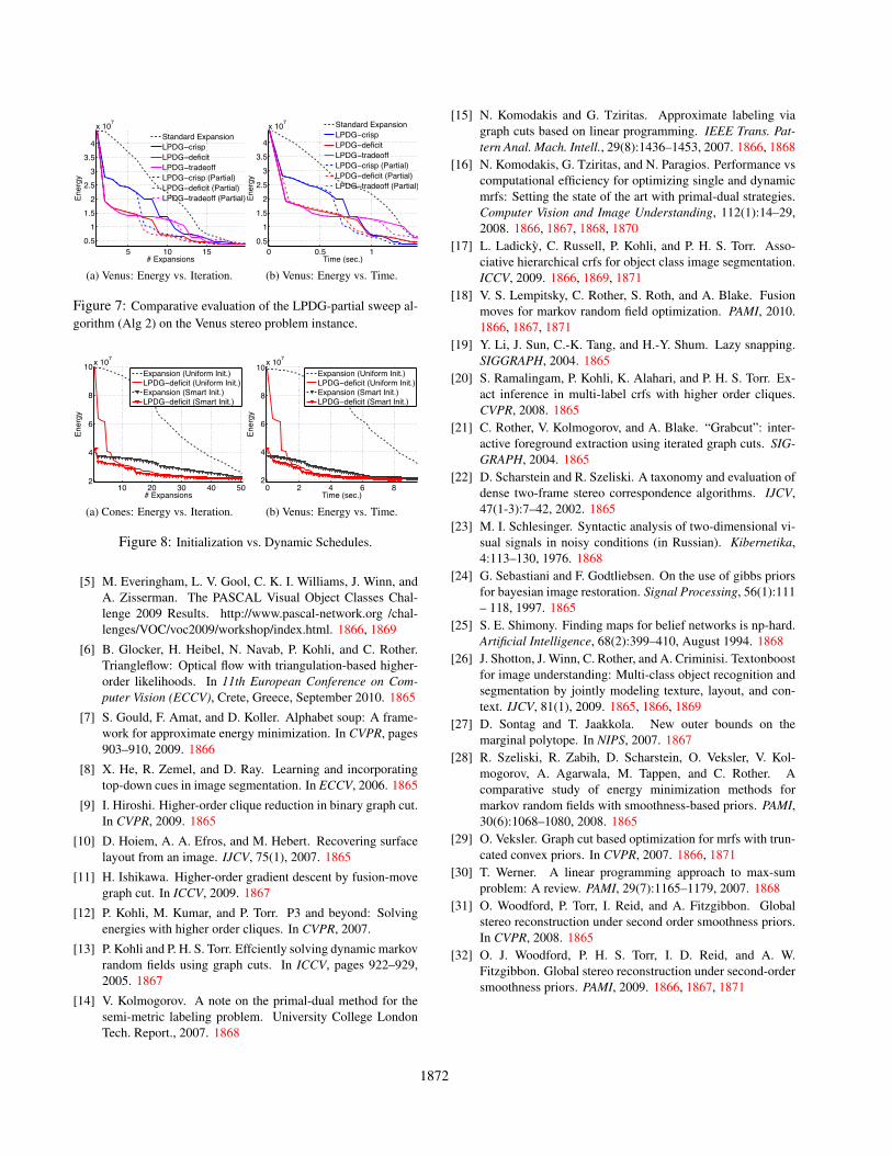
plots for stereo problems, while Fig. 2 and 6 shows the samefor object segmentation problems. We can see that in allcases LPDG-based dynamic label schedules perform signif-icantly better than the standard static schedules. For mostproblem instances, our guided approach can reduce the run-ning time by more than 50%.Complete vs Partial Label Sweep. We experimented withpartial sweeps but on Pascal it performed very similar to thefull sweep algorithm, which also converges very quickly.We believe the reason for this is that the energies are fairlyconfident, and most labels are only expanded on once. OnStereo, we were able to observe improvement of partialsweeps over full sweeps, typically by 10-20%. We believeproblems with extremely large label spaces where individ-ual instances contain only a small subset of these labelswould most benefit from our partial sweep algorithm. Fig. 7shows performance of all scoring function for full and par-tial sweep on the Venus stereo problem.Initialization vs. Dynamic Schedules. For all methodspresented in this paper, we initialized the primal labellinguniformly with ones, i.e. xpi = 1, ∀i ∈ [n]. Of course, abetter initialization scheme based on unary potentials mighthelp, e.g., we can initialize with the labels that minimizenode energies independently, i.e. xi = argmins∈L θi(s).However, we found in our experiments that even with abad uniform initialization, LPDG-based methods outper-formed standard Expansion with a good initialization basedon unary potentials. This demonstrates the power of LPDGbased dynamic scheduling. Of course, ideally we shoulduse both a good initialization and a good dynamic schedul-ing scheme. Fig. 8 shows the results.
6. Conclusions
We presented a novel method for proposing good ex-pansion moves that significantly speeds up the Expansionand FAST-PD energy minimization algorithms. The results
1870

(a) Cones: Image. (b) Cones: Predicted Disparity.
0 20 40 60
23456789
x 107
# Expansions
Ener
gy
Standard ExpansionLPDG crispLPDG deficitLPDG tradeoff
(c) Cones: Energy vs. Iterations.
0 2 4 6
2
4
6
8
10x 107
Time (sec.)
Ener
gy
Standard ExpansionLPDG crispLPDG deficitLPDG tradeoff
(d) Cones: Energy vs. Time.
0 20 40 60 80 100
2
3
4
5
6
7
x 107
# Expansions
Ener
gy
Standard ExpansionLPDG crispLPDG deficitLPDG tradeoff
(e) Teddy: Energy vs. Iterations.
0 2 4 6 81
2
3
4
5
6
7
8x 10⁷
Time (sec.)
Ener
gy
Standard ExpansionLPDG crispLPDG deficitLPDG tradeoff
(f) Teddy: Energy vs. Time.
5 10 15 20 25 300.5
11.5
22.5
33.5
4
x 107
# Expansions
Ener
gy
Standard ExpansionLPDG crispLPDG deficitLPDG tradeoff
(g) Venus: Energy vs. Iterations.
0 1 2 30
1
2
3
4
x 107
Time (sec.)
Ener
gy
Standard ExpansionLPDG crispLPDG deficitLPDG tradeoff
(h) Venus: Energy vs. Time.
Figure 5: Results on energy functions used for Stereo-Matching. (a) Cones image from the Middlebury Stereo Dataset. (b) The computeddisparity map by minimizing the energy used in [1]. (c) Graph showing how the energy of the solution changes with number of expansionsof the different variants of guided Expansions and standard FAST-PD. (d) Graph showing how the energy of the solution obtained bydifferent variants of guided Expansion and FAST-PD changes with running time. (e) and (f) Results for Teddy image pair. (g) and (h)Results for Venus image pair.
(a) Image.
0 20 40
1.2
1.25
1.3
x 108
# Expansions
Ener
gy
Standard Exp.LPDG crispLPDG deficitLPDG tradeoff
(b) Energy vs. Iterations.
0 1 2 3
1.2
1.25
1.3
x 108
Time (sec.)
Ener
gy
Standard Exp.LPDG crispLPDG deficitLPDG tradeoff
(c) Energy vs. Time. (d) Segmentation.
Figure 6: Results on energy functions used for Object Segmentation. (a) Image from the PASCAL VOC 2009 dataset. (b) Solutionobtained by minimizing the pairwise energy function used in [17]. (c) Graph showing how the energy of the solution changes with numberof expansions of the different variants of guided Expansions and standard FAST-PD. (d) Graph showing how the energy of the solutionobtained by different variants of guided Expansion and FAST-PD changes with running time.
of our experiments have demonstrated that primal and dualsolutions can be used to make good predictions on whichlabel-expansion will lead to lower energy solutions. We be-lieve that the theory developed in this paper, and our methodwill help significantly reduce the time taken for energy min-imization in problems which are defined over large labelsets (e.g. denoising).
This paper focused on developing the LPDG-based rank-ing scores for Expansion moves. Extending these ideas togeneral moves like Range [29] and Fusion [18, 32] is an in-teresting direction for future work.
References[1] K. Alahari, P. Kohli, and P. H. S. Torr. Dynamic hy-
brid algorithms for map inference in discrete mrfs. PAMI,pages 1846–1857, 2010. http://cms.brookes.ac.uk/staff/Karteek/data.tgz. 1867, 1869, 1871
[2] D. Batra, A. Kowdle, D. Parikh, J. Luo, and T. Chen. icoseg:Interactive co-segmentation with intelligent scribble guid-ance. In CVPR, 2010. 1865
[3] Y. Boykov and M.-P. Jolly. Interactive graph cuts for optimalboundary and region segmentation of objects in n-d images.ICCV, 2001. 1865
[4] Y. Boykov, O. Veksler, and R. Zabih. Efficient approximateenergy minimization via graph cuts. PAMI, 20(12):1222–1239, 2001. 1865
1871
5 10 150.5
11.5
22.5
33.5
4
x 107
# Expansions
Ener
gy
Standard ExpansionLPDG crispLPDG deficitLPDG tradeoffLPDG crisp (Partial)LPDG deficit (Partial)LPDG tradeoff (Partial)
(a) Venus: Energy vs. Iteration.
0 0.5 10.5
11.5
22.5
33.5
4
x 107
Time (sec.)En
ergy
Standard ExpansionLPDG crispLPDG deficitLPDG tradeoffLPDG crisp (Partial)LPDG deficit (Partial)LPDG tradeoff (Partial)
(b) Venus: Energy vs. Time.
Figure 7: Comparative evaluation of the LPDG-partial sweep al-gorithm (Alg 2) on the Venus stereo problem instance.
10 20 30 40 502
4
6
8
10x 107
# Expansions
Ener
gy
Expansion (Uniform Init.)LPDG deficit (Uniform Init.)Expansion (Smart Init.)LPDG deficit (Smart Init.)
(a) Cones: Energy vs. Iteration.
0 2 4 6 82
4
6
8
10x 107
Time (sec.)
Ener
gy
Expansion (Uniform Init.)LPDG deficit (Uniform Init.)Expansion (Smart Init.)LPDG deficit (Smart Init.)
(b) Venus: Energy vs. Time.
Figure 8: Initialization vs. Dynamic Schedules.
[5] M. Everingham, L. V. Gool, C. K. I. Williams, J. Winn, andA. Zisserman. The PASCAL Visual Object Classes Chal-lenge 2009 Results. http://www.pascal-network.org /chal-lenges/VOC/voc2009/workshop/index.html. 1866, 1869
[6] B. Glocker, H. Heibel, N. Navab, P. Kohli, and C. Rother.Triangleflow: Optical flow with triangulation-based higher-order likelihoods. In 11th European Conference on Com-puter Vision (ECCV), Crete, Greece, September 2010. 1865
[7] S. Gould, F. Amat, and D. Koller. Alphabet soup: A frame-work for approximate energy minimization. In CVPR, pages903–910, 2009. 1866
[8] X. He, R. Zemel, and D. Ray. Learning and incorporatingtop-down cues in image segmentation. In ECCV, 2006. 1865
[9] I. Hiroshi. Higher-order clique reduction in binary graph cut.In CVPR, 2009. 1865
[10] D. Hoiem, A. A. Efros, and M. Hebert. Recovering surfacelayout from an image. IJCV, 75(1), 2007. 1865
[11] H. Ishikawa. Higher-order gradient descent by fusion-movegraph cut. In ICCV, 2009. 1867
[12] P. Kohli, M. Kumar, and P. Torr. P3 and beyond: Solvingenergies with higher order cliques. In CVPR, 2007.
[13] P. Kohli and P. H. S. Torr. Effciently solving dynamic markovrandom fields using graph cuts. In ICCV, pages 922–929,2005. 1867
[14] V. Kolmogorov. A note on the primal-dual method for thesemi-metric labeling problem. University College LondonTech. Report., 2007. 1868
[15] N. Komodakis and G. Tziritas. Approximate labeling viagraph cuts based on linear programming. IEEE Trans. Pat-tern Anal. Mach. Intell., 29(8):1436–1453, 2007. 1866, 1868
[16] N. Komodakis, G. Tziritas, and N. Paragios. Performance vscomputational efficiency for optimizing single and dynamicmrfs: Setting the state of the art with primal-dual strategies.Computer Vision and Image Understanding, 112(1):14–29,2008. 1866, 1867, 1868, 1870
[17] L. Ladicky, C. Russell, P. Kohli, and P. H. S. Torr. Asso-ciative hierarchical crfs for object class image segmentation.ICCV, 2009. 1866, 1869, 1871
[18] V. S. Lempitsky, C. Rother, S. Roth, and A. Blake. Fusionmoves for markov random field optimization. PAMI, 2010.1866, 1867, 1871
[19] Y. Li, J. Sun, C.-K. Tang, and H.-Y. Shum. Lazy snapping.SIGGRAPH, 2004. 1865
[20] S. Ramalingam, P. Kohli, K. Alahari, and P. H. S. Torr. Ex-act inference in multi-label crfs with higher order cliques.CVPR, 2008. 1865
[21] C. Rother, V. Kolmogorov, and A. Blake. “Grabcut”: inter-active foreground extraction using iterated graph cuts. SIG-GRAPH, 2004. 1865
[22] D. Scharstein and R. Szeliski. A taxonomy and evaluation ofdense two-frame stereo correspondence algorithms. IJCV,47(1-3):7–42, 2002. 1865
[23] M. I. Schlesinger. Syntactic analysis of two-dimensional vi-sual signals in noisy conditions (in Russian). Kibernetika,4:113–130, 1976. 1868
[24] G. Sebastiani and F. Godtliebsen. On the use of gibbs priorsfor bayesian image restoration. Signal Processing, 56(1):111– 118, 1997. 1865
[25] S. E. Shimony. Finding maps for belief networks is np-hard.Artificial Intelligence, 68(2):399–410, August 1994. 1868
[26] J. Shotton, J. Winn, C. Rother, and A. Criminisi. Textonboostfor image understanding: Multi-class object recognition andsegmentation by jointly modeling texture, layout, and con-text. IJCV, 81(1), 2009. 1865, 1866, 1869
[27] D. Sontag and T. Jaakkola. New outer bounds on themarginal polytope. In NIPS, 2007. 1867
[28] R. Szeliski, R. Zabih, D. Scharstein, O. Veksler, V. Kol-mogorov, A. Agarwala, M. Tappen, and C. Rother. Acomparative study of energy minimization methods formarkov random fields with smoothness-based priors. PAMI,30(6):1068–1080, 2008. 1865
[29] O. Veksler. Graph cut based optimization for mrfs with trun-cated convex priors. In CVPR, 2007. 1866, 1871
[30] T. Werner. A linear programming approach to max-sumproblem: A review. PAMI, 29(7):1165–1179, 2007. 1868
[31] O. Woodford, P. Torr, I. Reid, and A. Fitzgibbon. Globalstereo reconstruction under second order smoothness priors.In CVPR, 2008. 1865
[32] O. J. Woodford, P. H. S. Torr, I. D. Reid, and A. W.Fitzgibbon. Global stereo reconstruction under second-ordersmoothness priors. PAMI, 2009. 1866, 1867, 1871
1872